Analysis of Algorithm Efficiency
Dr. Yingwu Zhu
p5-11, p16-29, p43-53, p93-96
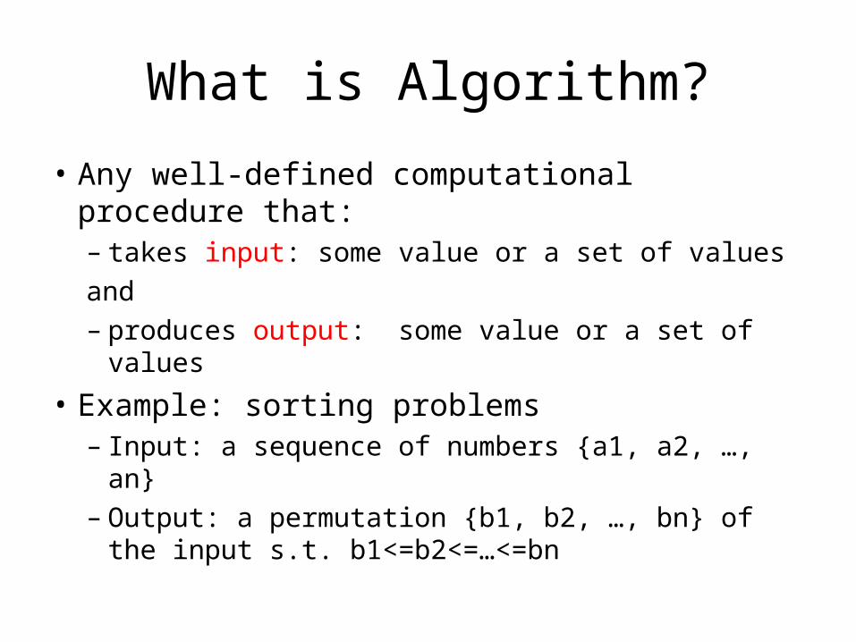
What is Algorithm?
• Any well-defined computational procedure that:– takes input: some value or a set of values and– produces output: some value or a set of values
• Example: sorting problems– Input: a sequence of numbers {a1, a2, …, an}– Output: a permutation {b1, b2, …, bn} of the input
s.t. b1<=b2<=…<=bn
Algorithms: Motivation
• At the heart of programs lie algorithms• Algorithms as a key technology• Think about:
– mapping/navigation– Google search– word processing (spelling correction, layout…)– content delivery and streaming video– games (graphics, rendering…)– big data (querying, learning…)
Algorithms: Motivation
• In a perfect world– for each problem we would have an algorithm– the algorithm would be the fastest possible
What would CS look like in this world?
Algorithms: Motivation
• Our world (fortunately) is not so perfect:– for many problems we know embarrassingly little
about what the fastest algorithm is• multiplying two integers or two matrices• factoring an integer into primes• determining shortest tour of given n cities
– for many problems we suspect fast algorithms are impossible (NP-complete problems)
– for some problems we have unexpected and clever algorithms (we will see many of these)
Analyzing Algorithms
• Given computing resources and input data– how fast does an algorithm run?
• Time efficiency: amount of time required to accomplish the task
• Our focus
– How much memory is required?• Space efficiency: amount of memory required • Deals with the extra space the algorithm requires
Time Efficiency
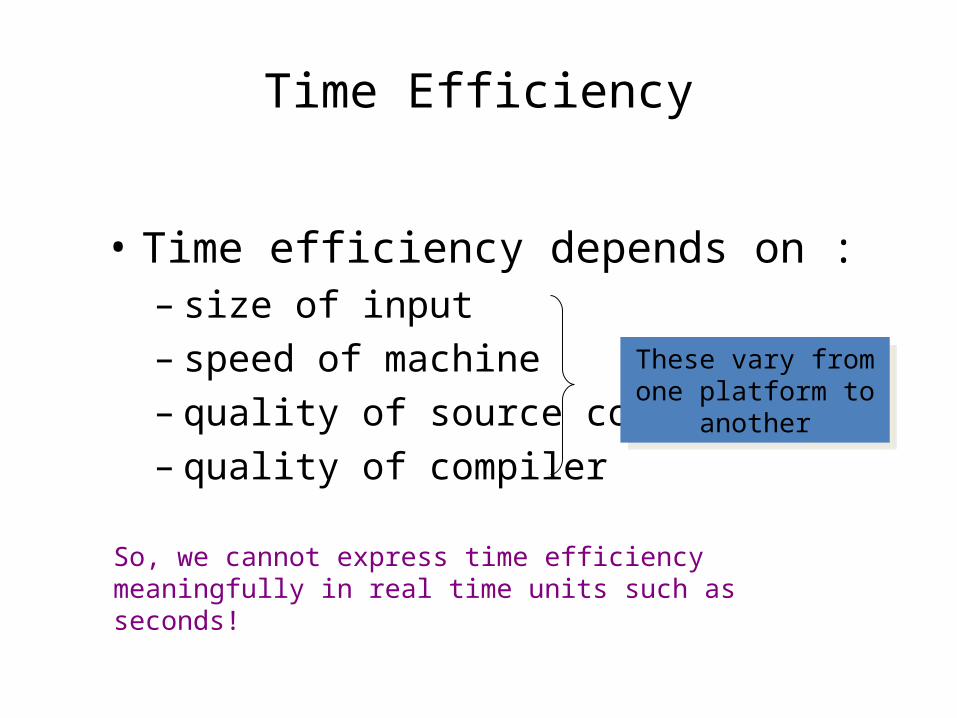
• Time efficiency depends on :– size of input– speed of machine – quality of source code– quality of compiler
These vary from one platform to another
These vary from one platform to another
So, we cannot express time efficiency meaningfully in real time units such as seconds!
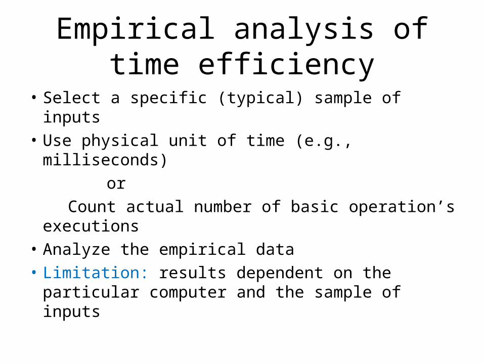
Empirical analysis of time efficiency
• Select a specific (typical) sample of inputs• Use physical unit of time (e.g., milliseconds) or Count actual number of basic operation’s
executions• Analyze the empirical data• Limitation: results dependent on the
particular computer and the sample of inputs
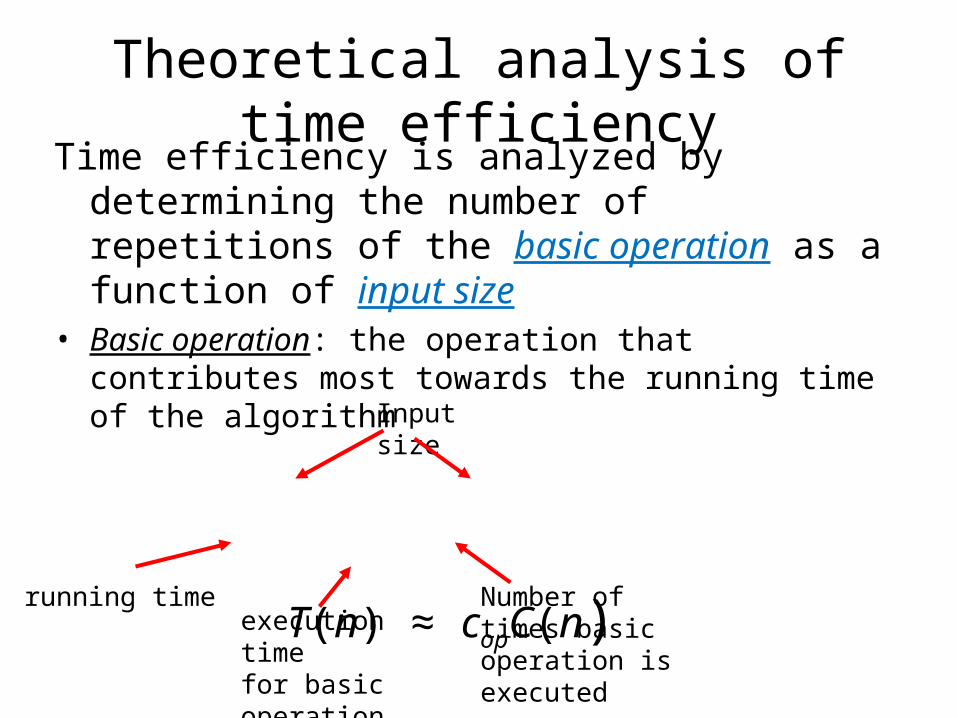
Theoretical analysis of time efficiencyTime efficiency is analyzed by determining the number
of repetitions of the basic operation as a function of input size
• Basic operation: the operation that contributes most towards the running time of the algorithm
T(n) ≈ copC(n)running time
execution timefor basic operation
Number of times basic operation is executed
Input size
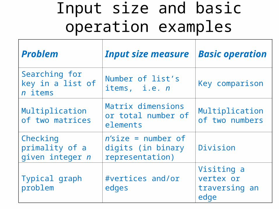
Input size and basic operation examples
Problem Input size measure Basic operation
Searching for key in a list of n items
Number of list’s items, i.e. n
Key comparison
Multiplication of two matrices
Matrix dimensions or total number of elements
Multiplication of two numbers
Checking primality of a given integer n
n’size = number of digits (in binary representation)
Division
Typical graph problem #vertices and/or edgesVisiting a vertex or traversing an edge
Time Efficiency
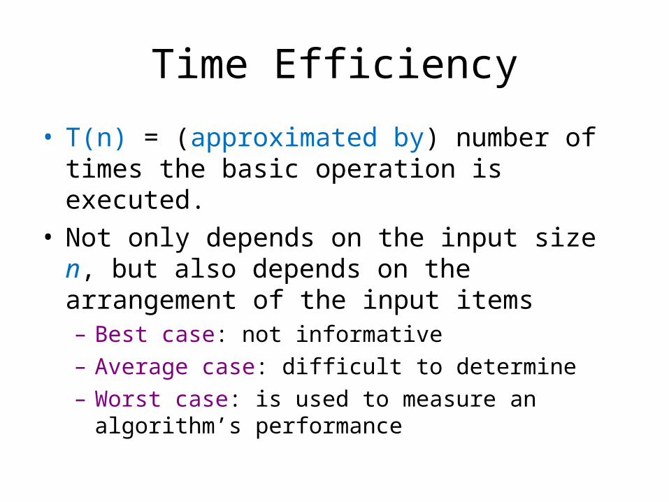
• T(n) = (approximated by) number of times the basic operation is executed.
• Not only depends on the input size n, but also depends on the arrangement of the input items– Best case: not informative– Average case: difficult to determine– Worst case: is used to measure an algorithm’s
performance
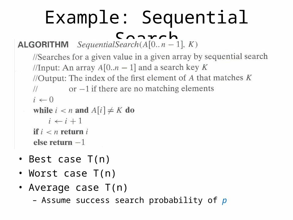
Example: Sequential Search
• Best case T(n)• Worst case T(n)• Average case T(n)
– Assume success search probability of p
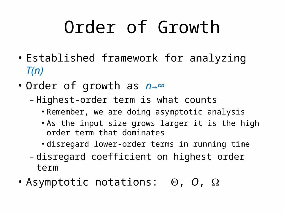
Order of Growth
• Established framework for analyzing T(n)• Order of growth as n→∞
– Highest-order term is what counts• Remember, we are doing asymptotic analysis• As the input size grows larger it is the high order term
that dominates• disregard lower-order terms in running time
– disregard coefficient on highest order term
• Asymptotic notations: , O,
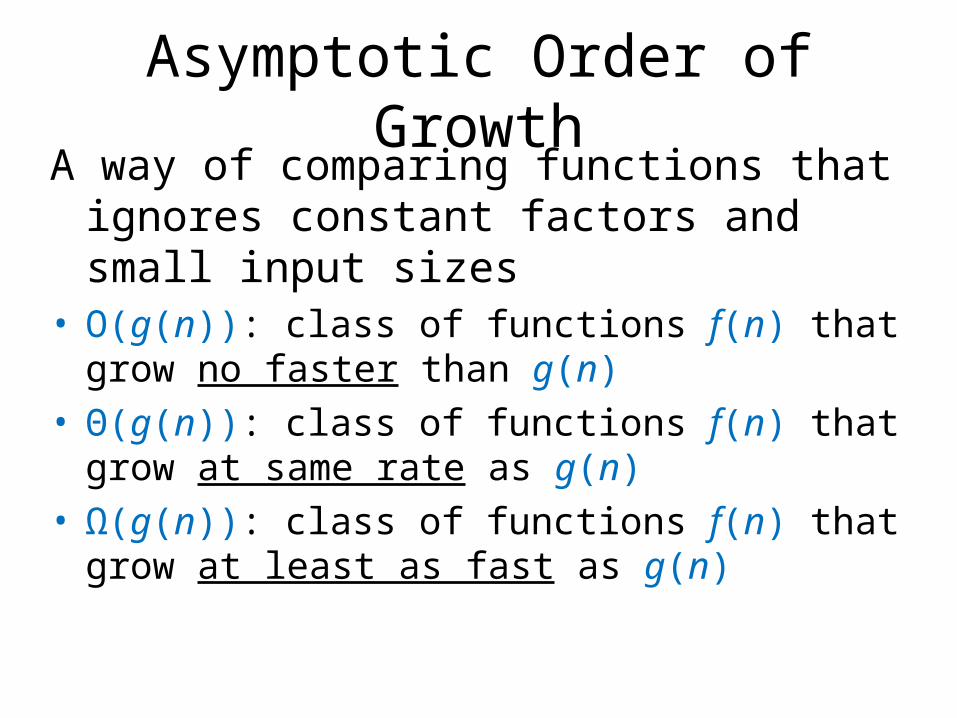
Asymptotic Order of GrowthA way of comparing functions that ignores constant
factors and small input sizes• O(g(n)): class of functions f(n) that grow no faster than
g(n)• Θ(g(n)): class of functions f(n) that grow at same rate as
g(n)• Ω(g(n)): class of functions f(n) that grow at least as fast
as g(n)
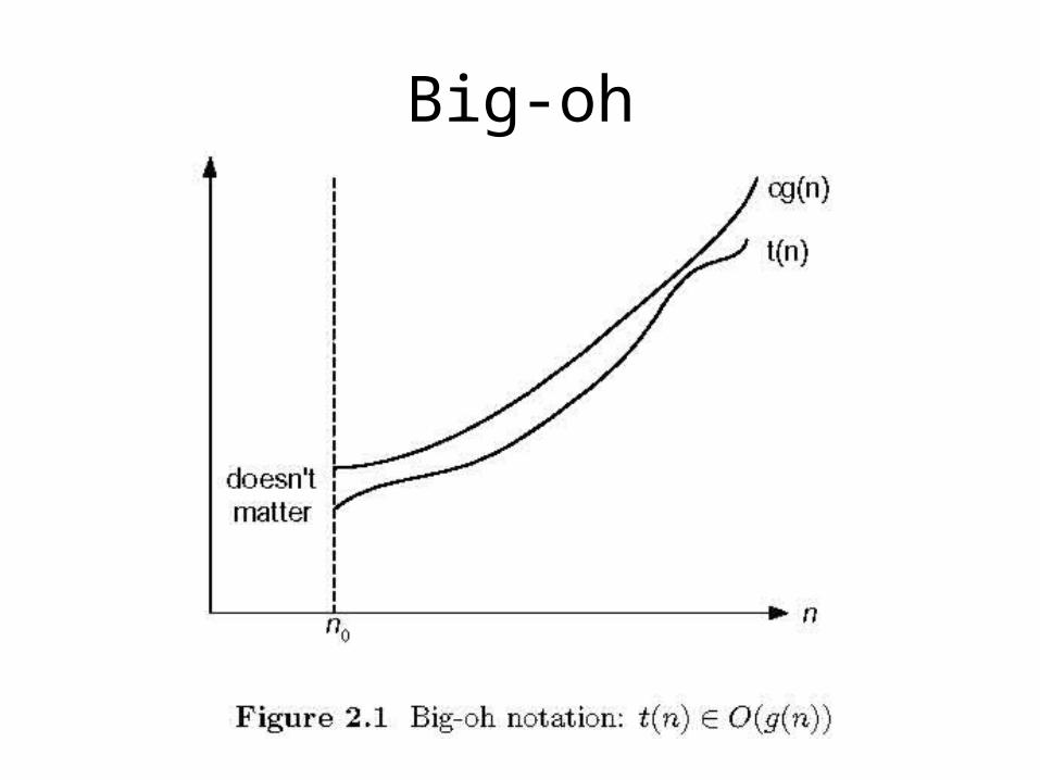
Big-oh
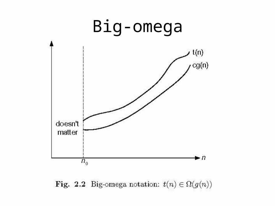
Big-omega
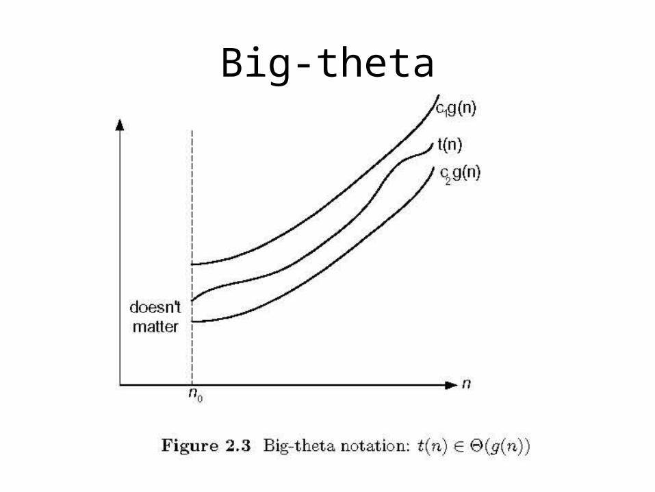
Big-theta
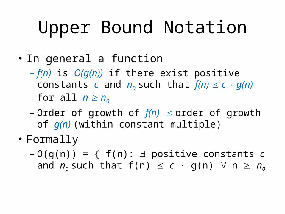
Upper Bound Notation
• In general a function– f(n) is O(g(n)) if there exist positive constants c
and n0 such that f(n) c g(n) for all n n0
– Order of growth of f(n) order of growth of g(n) (within constant multiple)
• Formally– O(g(n)) = { f(n): positive constants c and n0 such
that f(n) c g(n) n n0
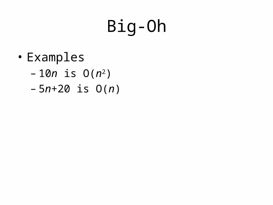
Big-Oh
• Examples– 10n is O(n2)– 5n+20 is O(n)
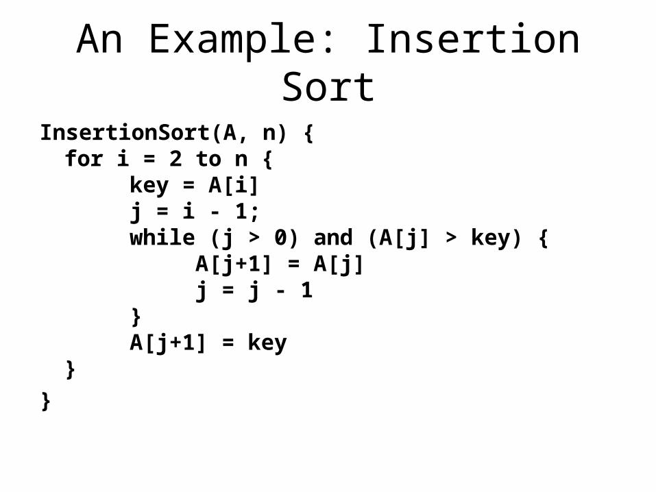
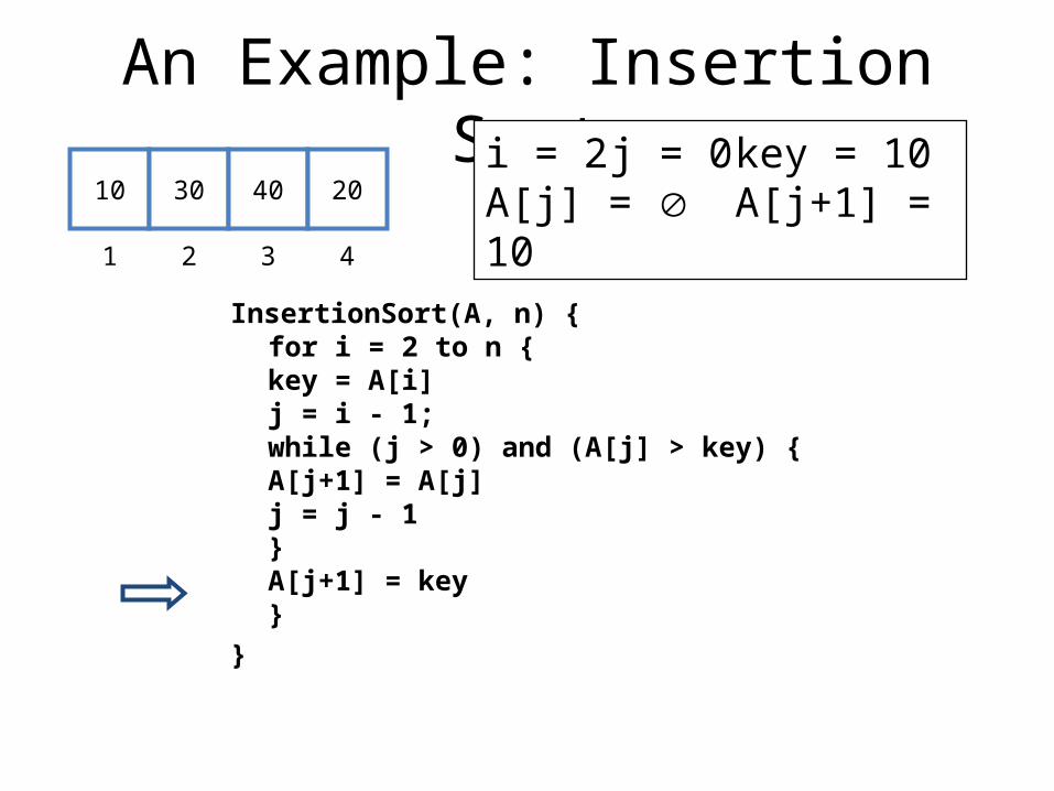
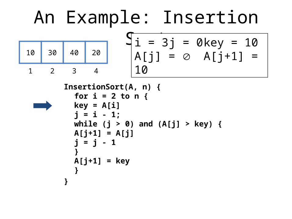
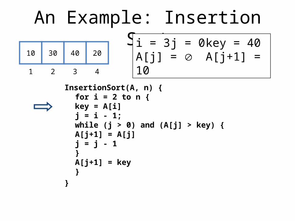
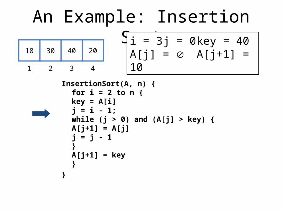
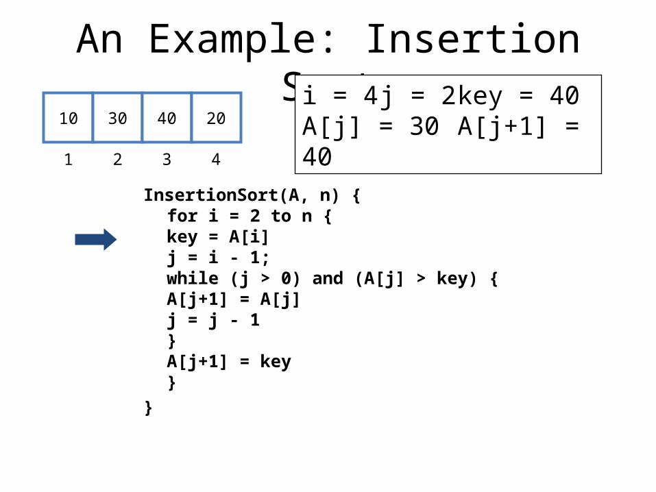
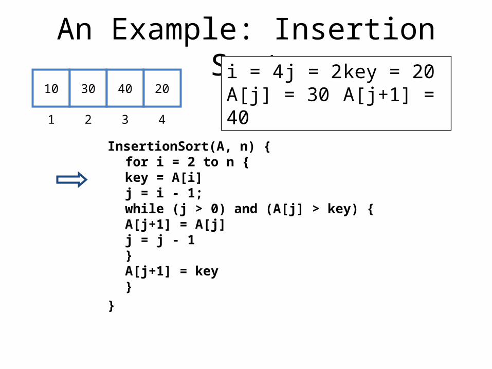
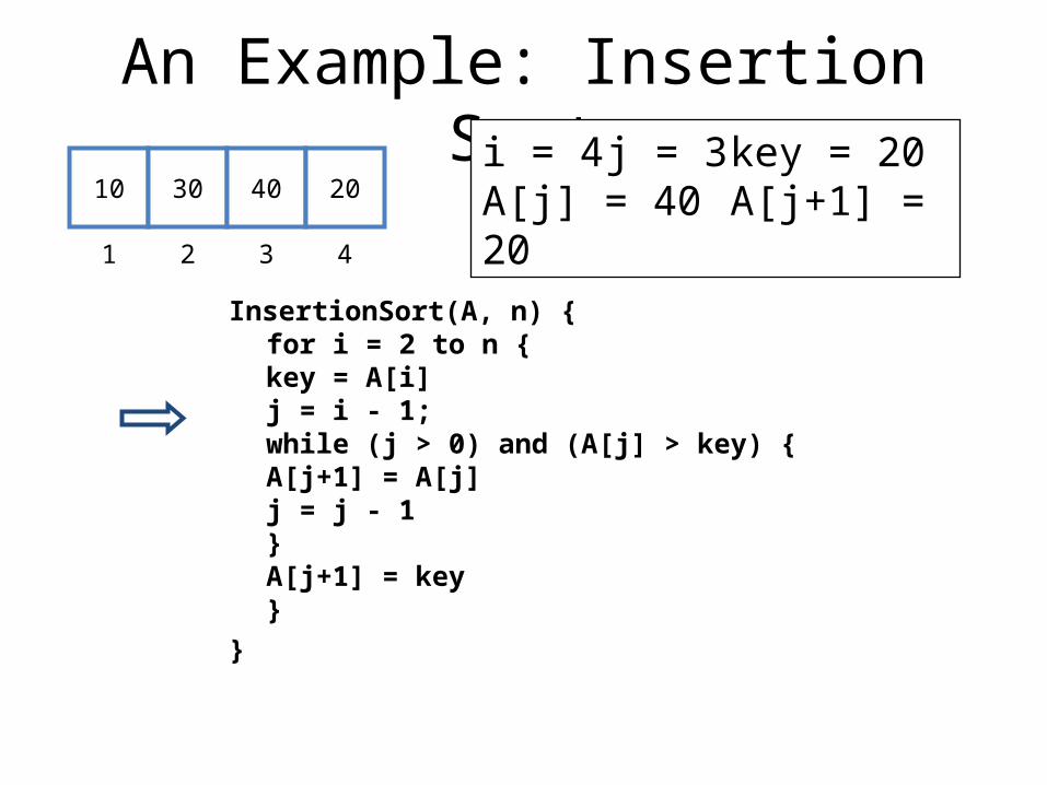
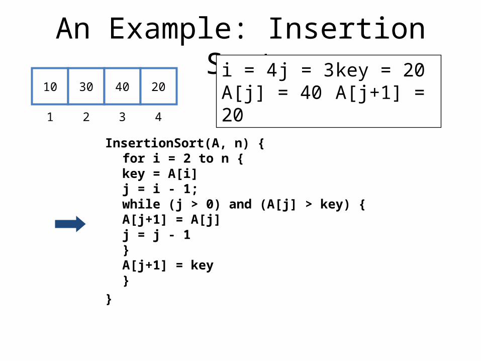
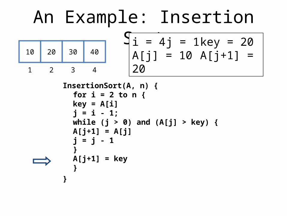
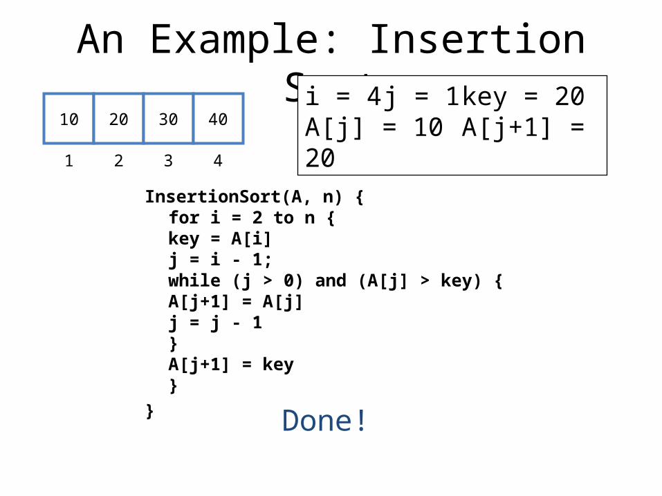
An Example: Insertion Sort
InsertionSort(A, n) {for i = 2 to n {
key = A[i]j = i - 1;while (j > 0) and (A[j] > key) {
A[j+1] = A[j]j = j - 1
}A[j+1] = key
}
}
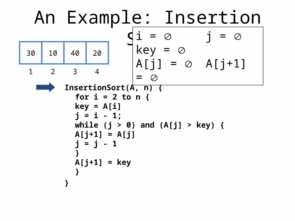
An Example: Insertion Sort
InsertionSort(A, n) {for i = 2 to n {
key = A[i]j = i - 1;while (j > 0) and (A[j] > key) {
A[j+1] = A[j]j = j - 1
}A[j+1] = key
}
}
30 10 40 20
1 2 3 4
i = j = key = A[j] = A[j+1] =

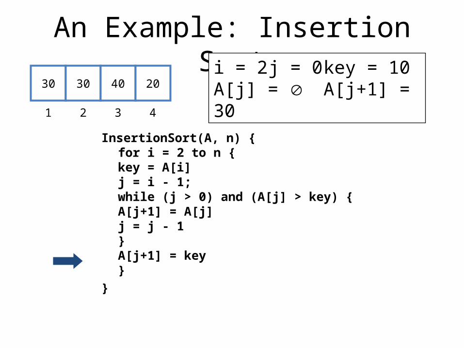
An Example: Insertion Sort
InsertionSort(A, n) {for i = 2 to n {
key = A[i]j = i - 1;while (j > 0) and (A[j] > key) {
A[j+1] = A[j]j = j - 1
}A[j+1] = key
}
}
30 10 40 20
1 2 3 4
i = 2 j = 1 key = 10A[j] = 30 A[j+1] = 10

An Example: Insertion Sort
InsertionSort(A, n) {for i = 2 to n {
key = A[i]j = i - 1;while (j > 0) and (A[j] > key) {
A[j+1] = A[j]j = j - 1
}A[j+1] = key
}
}
30 30 40 20
1 2 3 4
i = 2 j = 1 key = 10A[j] = 30 A[j+1] = 30

An Example: Insertion Sort
InsertionSort(A, n) {for i = 2 to n {
key = A[i]j = i - 1;while (j > 0) and (A[j] > key) {
A[j+1] = A[j]j = j - 1
}A[j+1] = key
}
}
30 30 40 20
1 2 3 4
i = 2 j = 1 key = 10A[j] = 30 A[j+1] = 30

An Example: Insertion Sort
InsertionSort(A, n) {for i = 2 to n {
key = A[i]j = i - 1;while (j > 0) and (A[j] > key) {
A[j+1] = A[j]j = j - 1
}A[j+1] = key
}
}
30 30 40 20
1 2 3 4
i = 2 j = 0 key = 10A[j] = A[j+1] = 30
An Example: Insertion Sort
InsertionSort(A, n) {for i = 2 to n {
key = A[i]j = i - 1;while (j > 0) and (A[j] > key) {
A[j+1] = A[j]j = j - 1
}A[j+1] = key
}
}
30 30 40 20
1 2 3 4
i = 2 j = 0 key = 10A[j] = A[j+1] = 30
An Example: Insertion Sort
InsertionSort(A, n) {for i = 2 to n {
key = A[i]j = i - 1;while (j > 0) and (A[j] > key) {
A[j+1] = A[j]j = j - 1
}A[j+1] = key
}
}
10 30 40 20
1 2 3 4
i = 2 j = 0 key = 10A[j] = A[j+1] = 10
An Example: Insertion Sort
InsertionSort(A, n) {for i = 2 to n {
key = A[i]j = i - 1;while (j > 0) and (A[j] > key) {
A[j+1] = A[j]j = j - 1
}A[j+1] = key
}
}
10 30 40 20
1 2 3 4
i = 3 j = 0 key = 10A[j] = A[j+1] = 10
An Example: Insertion Sort
InsertionSort(A, n) {for i = 2 to n {
key = A[i]j = i - 1;while (j > 0) and (A[j] > key) {
A[j+1] = A[j]j = j - 1
}A[j+1] = key
}
}
10 30 40 20
1 2 3 4
i = 3 j = 0 key = 40A[j] = A[j+1] = 10
An Example: Insertion Sort
InsertionSort(A, n) {for i = 2 to n {
key = A[i]j = i - 1;while (j > 0) and (A[j] > key) {
A[j+1] = A[j]j = j - 1
}A[j+1] = key
}
}
10 30 40 20
1 2 3 4
i = 3 j = 0 key = 40A[j] = A[j+1] = 10

An Example: Insertion Sort
InsertionSort(A, n) {for i = 2 to n {
key = A[i]j = i - 1;while (j > 0) and (A[j] > key) {
A[j+1] = A[j]j = j - 1
}A[j+1] = key
}
}
10 30 40 20
1 2 3 4
i = 3 j = 2 key = 40A[j] = 30 A[j+1] = 40

An Example: Insertion Sort
InsertionSort(A, n) {for i = 2 to n {
key = A[i]j = i - 1;while (j > 0) and (A[j] > key) {
A[j+1] = A[j]j = j - 1
}A[j+1] = key
}
}
10 30 40 20
1 2 3 4
i = 3 j = 2 key = 40A[j] = 30 A[j+1] = 40

An Example: Insertion Sort
InsertionSort(A, n) {for i = 2 to n {
key = A[i]j = i - 1;while (j > 0) and (A[j] > key) {
A[j+1] = A[j]j = j - 1
}A[j+1] = key
}
}
10 30 40 20
1 2 3 4
i = 3 j = 2 key = 40A[j] = 30 A[j+1] = 40
An Example: Insertion Sort
InsertionSort(A, n) {for i = 2 to n {
key = A[i]j = i - 1;while (j > 0) and (A[j] > key) {
A[j+1] = A[j]j = j - 1
}A[j+1] = key
}
}
10 30 40 20
1 2 3 4
i = 4 j = 2 key = 40A[j] = 30 A[j+1] = 40
An Example: Insertion Sort
InsertionSort(A, n) {for i = 2 to n {
key = A[i]j = i - 1;while (j > 0) and (A[j] > key) {
A[j+1] = A[j]j = j - 1
}A[j+1] = key
}
}
10 30 40 20
1 2 3 4
i = 4 j = 2 key = 20A[j] = 30 A[j+1] = 40

An Example: Insertion Sort
InsertionSort(A, n) {for i = 2 to n {
key = A[i]j = i - 1;while (j > 0) and (A[j] > key) {
A[j+1] = A[j]j = j - 1
}A[j+1] = key
}
}
10 30 40 20
1 2 3 4
i = 4 j = 2 key = 20A[j] = 30 A[j+1] = 40
An Example: Insertion Sort
InsertionSort(A, n) {for i = 2 to n {
key = A[i]j = i - 1;while (j > 0) and (A[j] > key) {
A[j+1] = A[j]j = j - 1
}A[j+1] = key
}
}
10 30 40 20
1 2 3 4
i = 4 j = 3 key = 20A[j] = 40 A[j+1] = 20
An Example: Insertion Sort
InsertionSort(A, n) {for i = 2 to n {
key = A[i]j = i - 1;while (j > 0) and (A[j] > key) {
A[j+1] = A[j]j = j - 1
}A[j+1] = key
}
}
10 30 40 20
1 2 3 4
i = 4 j = 3 key = 20A[j] = 40 A[j+1] = 20

An Example: Insertion Sort
InsertionSort(A, n) {for i = 2 to n {
key = A[i]j = i - 1;while (j > 0) and (A[j] > key) {
A[j+1] = A[j]j = j - 1
}A[j+1] = key
}
}
10 30 40 40
1 2 3 4
i = 4 j = 3 key = 20A[j] = 40 A[j+1] = 40

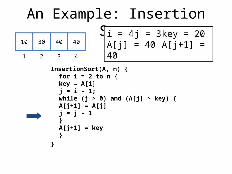
An Example: Insertion Sort
InsertionSort(A, n) {for i = 2 to n {
key = A[i]j = i - 1;while (j > 0) and (A[j] > key) {
A[j+1] = A[j]j = j - 1
}A[j+1] = key
}
}
10 30 40 40
1 2 3 4
i = 4 j = 3 key = 20A[j] = 40 A[j+1] = 40
An Example: Insertion Sort
InsertionSort(A, n) {for i = 2 to n {
key = A[i]j = i - 1;while (j > 0) and (A[j] > key) {
A[j+1] = A[j]j = j - 1
}A[j+1] = key
}
}
10 30 40 40
1 2 3 4
i = 4 j = 3 key = 20A[j] = 40 A[j+1] = 40

An Example: Insertion Sort
InsertionSort(A, n) {for i = 2 to n {
key = A[i]j = i - 1;while (j > 0) and (A[j] > key) {
A[j+1] = A[j]j = j - 1
}A[j+1] = key
}
}
10 30 40 40
1 2 3 4
i = 4 j = 2 key = 20A[j] = 30 A[j+1] = 40

An Example: Insertion Sort
InsertionSort(A, n) {for i = 2 to n {
key = A[i]j = i - 1;while (j > 0) and (A[j] > key) {
A[j+1] = A[j]j = j - 1
}A[j+1] = key
}
}
10 30 40 40
1 2 3 4
i = 4 j = 2 key = 20A[j] = 30 A[j+1] = 40
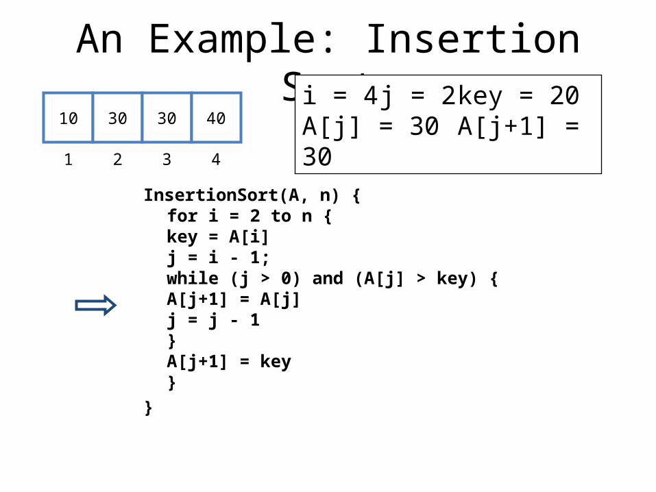
An Example: Insertion Sort
InsertionSort(A, n) {for i = 2 to n {
key = A[i]j = i - 1;while (j > 0) and (A[j] > key) {
A[j+1] = A[j]j = j - 1
}A[j+1] = key
}
}
10 30 30 40
1 2 3 4
i = 4 j = 2 key = 20A[j] = 30 A[j+1] = 30

An Example: Insertion Sort
InsertionSort(A, n) {for i = 2 to n {
key = A[i]j = i - 1;while (j > 0) and (A[j] > key) {
A[j+1] = A[j]j = j - 1
}A[j+1] = key
}
}
10 30 30 40
1 2 3 4
i = 4 j = 2 key = 20A[j] = 30 A[j+1] = 30
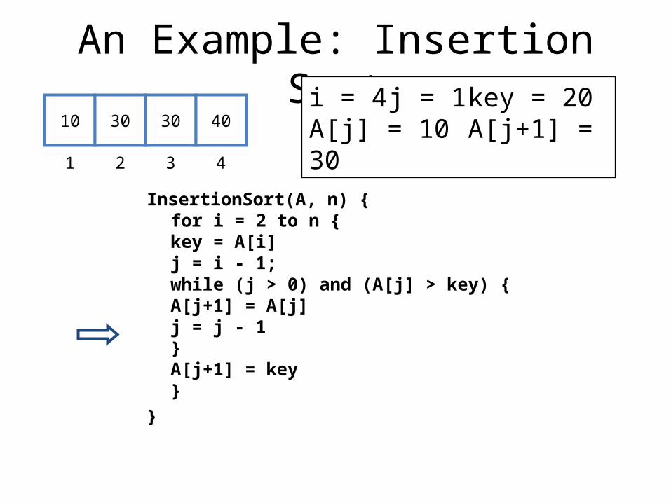
An Example: Insertion Sort
InsertionSort(A, n) {for i = 2 to n {
key = A[i]j = i - 1;while (j > 0) and (A[j] > key) {
A[j+1] = A[j]j = j - 1
}A[j+1] = key
}
}
10 30 30 40
1 2 3 4
i = 4 j = 1 key = 20A[j] = 10 A[j+1] = 30
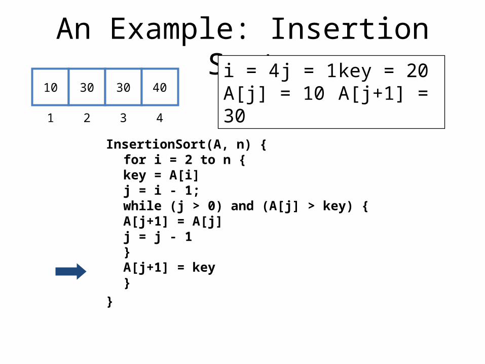
An Example: Insertion Sort
InsertionSort(A, n) {for i = 2 to n {
key = A[i]j = i - 1;while (j > 0) and (A[j] > key) {
A[j+1] = A[j]j = j - 1
}A[j+1] = key
}
}
10 30 30 40
1 2 3 4
i = 4 j = 1 key = 20A[j] = 10 A[j+1] = 30
An Example: Insertion Sort
InsertionSort(A, n) {for i = 2 to n {
key = A[i]j = i - 1;while (j > 0) and (A[j] > key) {
A[j+1] = A[j]j = j - 1
}A[j+1] = key
}
}
10 20 30 40
1 2 3 4
i = 4 j = 1 key = 20A[j] = 10 A[j+1] = 20
An Example: Insertion Sort
InsertionSort(A, n) {for i = 2 to n {
key = A[i]j = i - 1;while (j > 0) and (A[j] > key) {
A[j+1] = A[j]j = j - 1
}A[j+1] = key
}
}
10 20 30 40
1 2 3 4
i = 4 j = 1 key = 20A[j] = 10 A[j+1] = 20
Done!
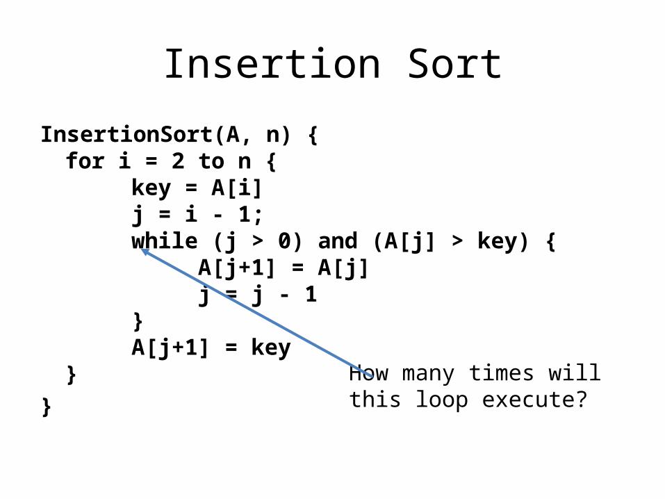
Insertion Sort
InsertionSort(A, n) {for i = 2 to n {
key = A[i]j = i - 1;while (j > 0) and (A[j] > key) {
A[j+1] = A[j]j = j - 1
}A[j+1] = key
}
}
How many times will this loop execute?
T(n) for Insertion Sort
• Worst case?• Best case?
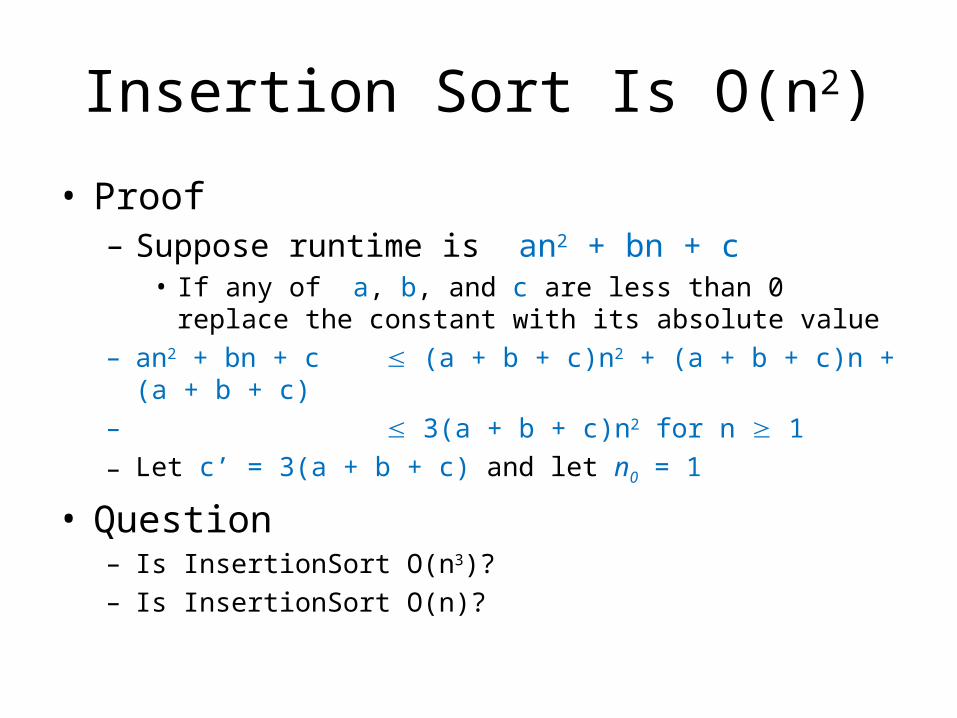
Insertion Sort Is O(n2)
• Proof– Suppose runtime is an2 + bn + c
• If any of a, b, and c are less than 0 replace the constant with its absolute value
– an2 + bn + c (a + b + c)n2 + (a + b + c)n + (a + b + c)– 3(a + b + c)n2 for n 1– Let c’ = 3(a + b + c) and let n0 = 1
• Question– Is InsertionSort O(n3)?– Is InsertionSort O(n)?
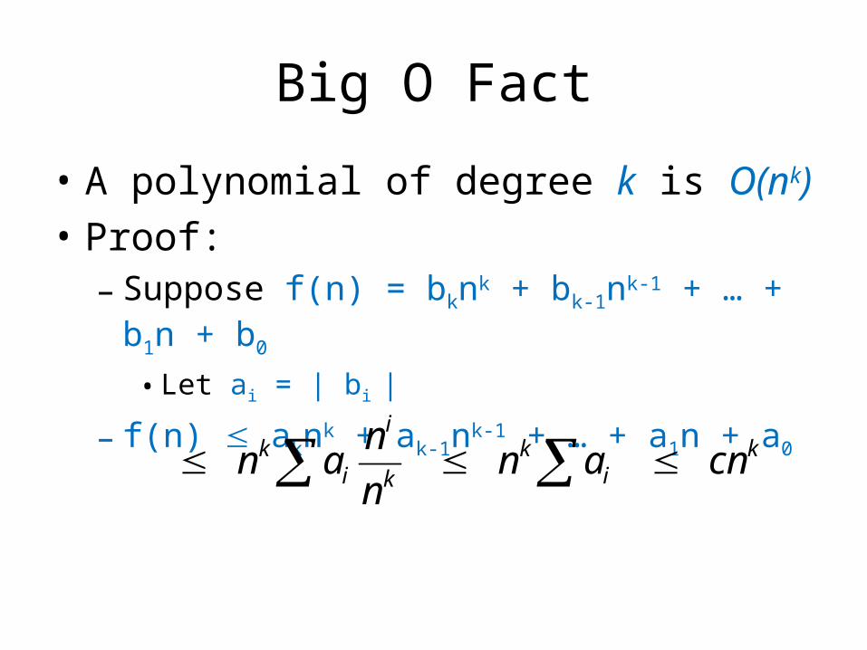
Big O Fact
• A polynomial of degree k is O(nk)• Proof:
– Suppose f(n) = bknk + bk-1nk-1 + … + b1n + b0
• Let ai = | bi |
– f(n) aknk + ak-1nk-1 + … + a1n + a0
ki
kk
i
ik cnan
n
nan
04/20/23
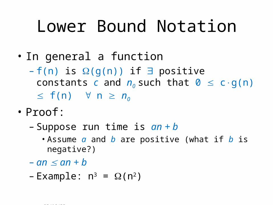
Lower Bound Notation
• In general a function– f(n) is (g(n)) if positive constants c and n0 such
that 0 cg(n) f(n) n n0
• Proof:– Suppose run time is an + b
• Assume a and b are positive (what if b is negative?)
– an an + b– Example: n3 = (n2)
04/20/23
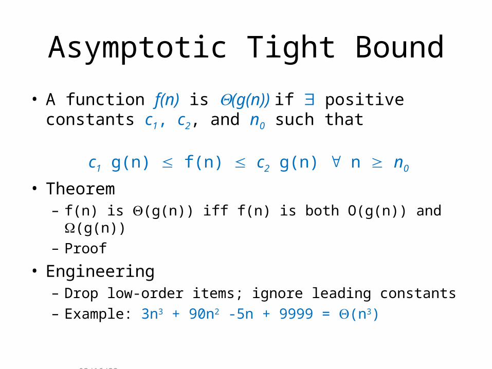
Asymptotic Tight Bound
• A function f(n) is (g(n)) if positive constants c1, c2, and n0 such that
c1 g(n) f(n) c2 g(n) n n0
• Theorem– f(n) is (g(n)) iff f(n) is both O(g(n)) and (g(n))– Proof
• Engineering– Drop low-order items; ignore leading constants– Example: 3n3 + 90n2 -5n + 9999 = (n3)
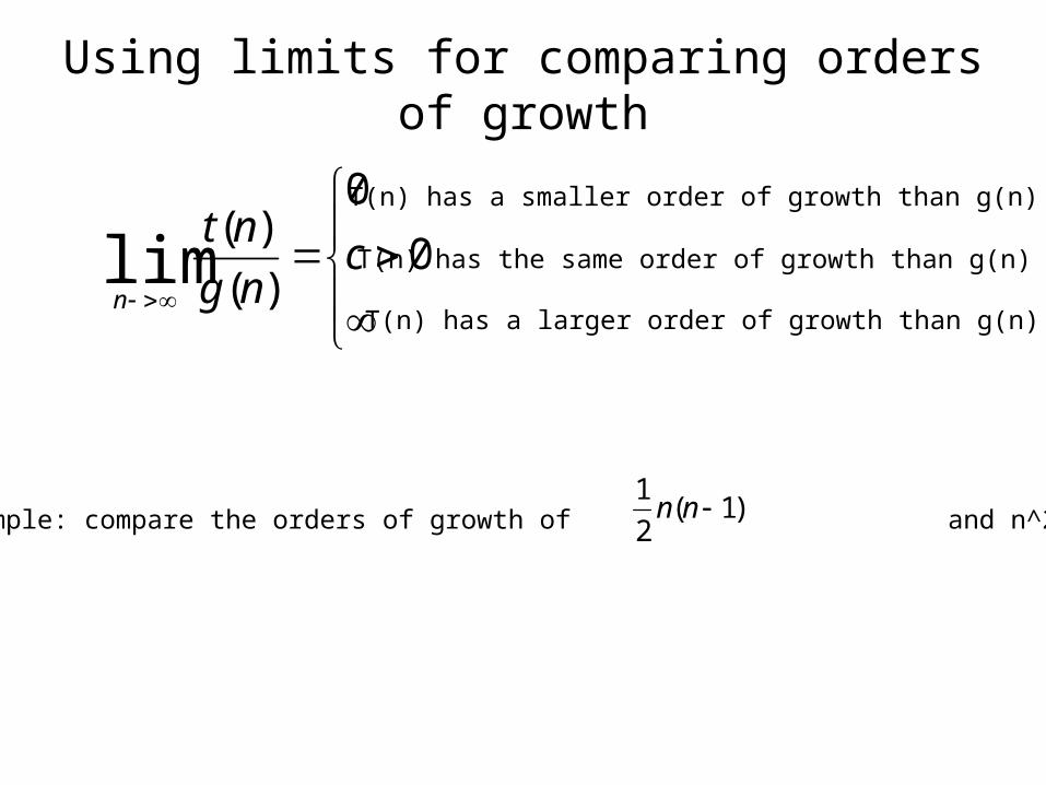
Using limits for comparing orders of growth
)1(2
1nn
0
0
)(
)(lim c
ng
nt
n
T(n) has a smaller order of growth than g(n)
T(n) has the same order of growth than g(n)
T(n) has a larger order of growth than g(n)
Example: compare the orders of growth of and n^2
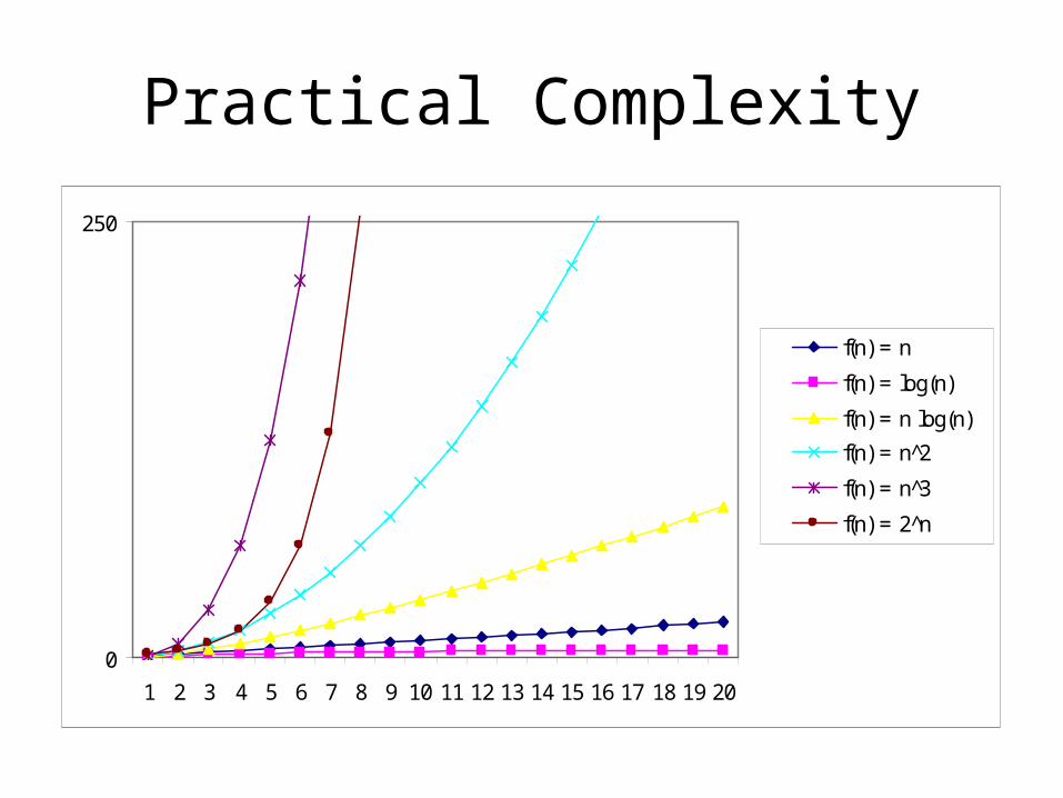
Practical Complexity
0
250
1 2 3 4 5 6 7 8 9 10 11 12 13 14 15 16 17 18 19 20
f(n) = n
f(n) = log(n)
f(n) = n log(n)
f(n) = n 2̂
f(n) = n 3̂
f(n) = 2 n̂
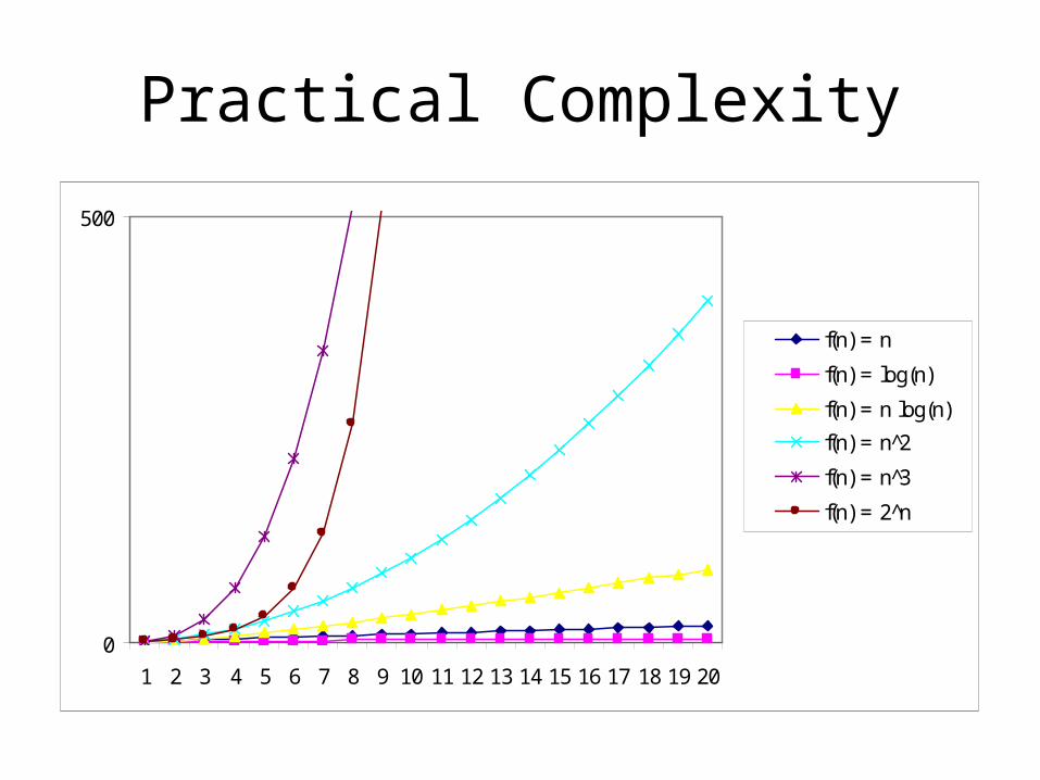
Practical Complexity
0
500
1 2 3 4 5 6 7 8 9 10 11 12 13 14 15 16 17 18 19 20
f(n) = n
f(n) = log(n)
f(n) = n log(n)
f(n) = n 2̂
f(n) = n 3̂
f(n) = 2 n̂
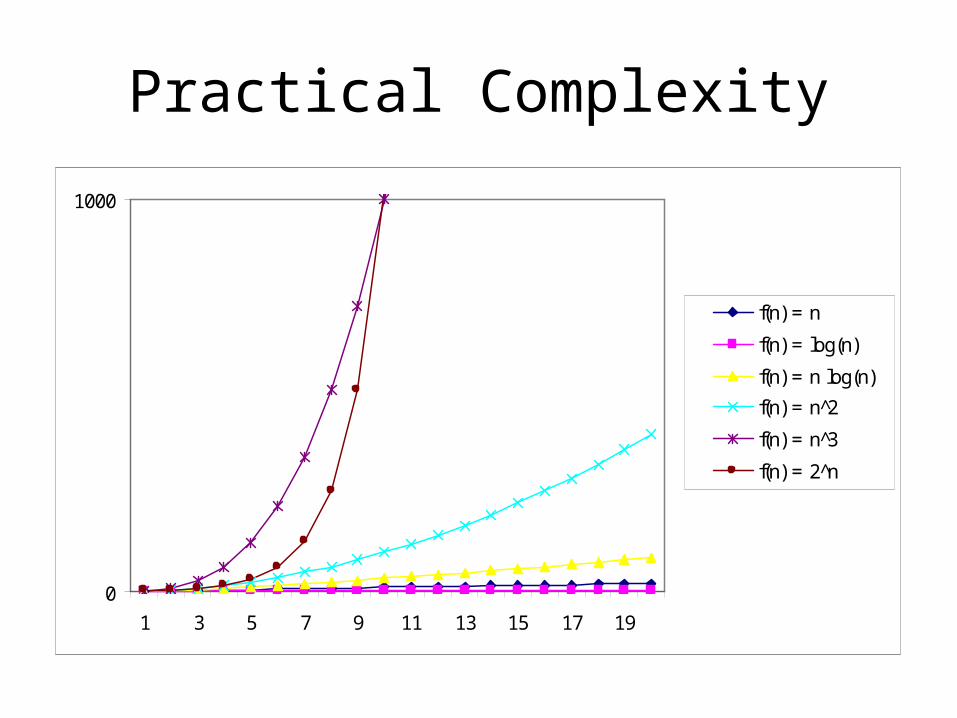
Practical Complexity
0
1000
1 3 5 7 9 11 13 15 17 19
f(n) = n
f(n) = log(n)
f(n) = n log(n)
f(n) = n 2̂
f(n) = n 3̂
f(n) = 2 n̂

David Luebke
60
04/20/23
Practical Complexity
0
1000
2000
3000
4000
5000
1 3 5 7 9 11 13 15 17 19
f(n) = n
f(n) = log(n)
f(n) = n log(n)
f(n) = n 2̂
f(n) = n 3̂
f(n) = 2 n̂
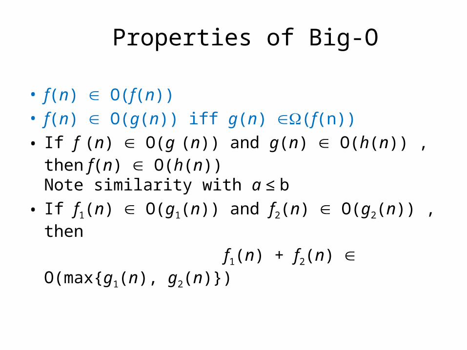
Properties of Big-O
• f(n) O(f(n))• f(n) O(g(n)) iff g(n) (f(n)) • If f (n) O(g (n)) and g(n) O(h(n)) , then f(n)
O(h(n)) Note similarity with a ≤ b
• If f1(n) O(g1(n)) and f2(n) O(g2(n)) , then
f1(n) + f2(n) O(max{g1(n), g2(n)})
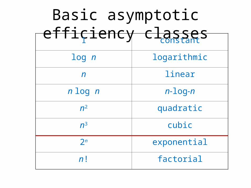
Basic asymptotic efficiency classes1 constant
log n logarithmic
n linear
n log n n-log-n
n2 quadratic
n3 cubic
2n exponential
n! factorial
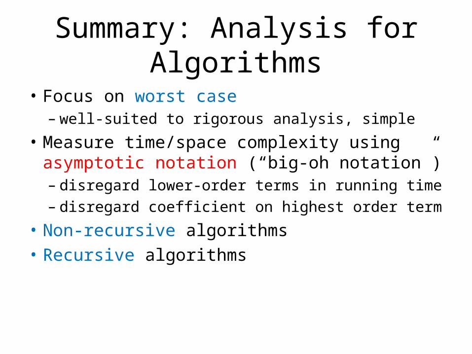
Summary: Analysis for Algorithms
• Focus on worst case– well-suited to rigorous analysis, simple
• Measure time/space complexity using asymptotic notation (“big-oh notation”)– disregard lower-order terms in running time– disregard coefficient on highest order term
• Non-recursive algorithms• Recursive algorithms
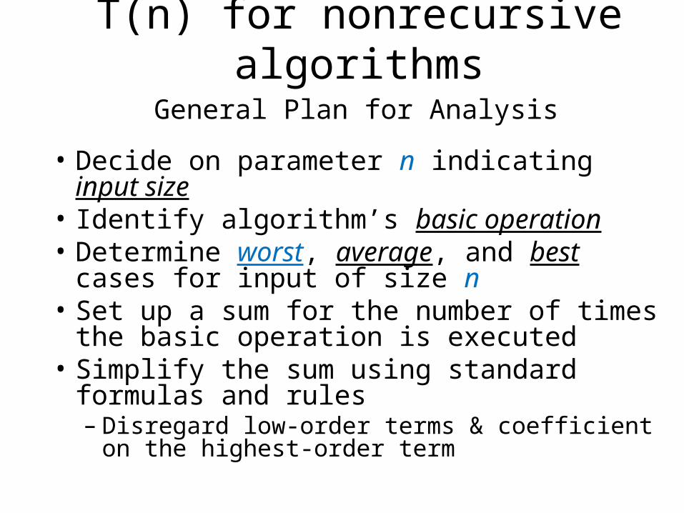
T(n) for nonrecursive algorithms
General Plan for Analysis
• Decide on parameter n indicating input size• Identify algorithm’s basic operation• Determine worst, average, and best cases for
input of size n• Set up a sum for the number of times the basic
operation is executed• Simplify the sum using standard formulas and
rules– Disregard low-order terms & coefficient on the
highest-order term
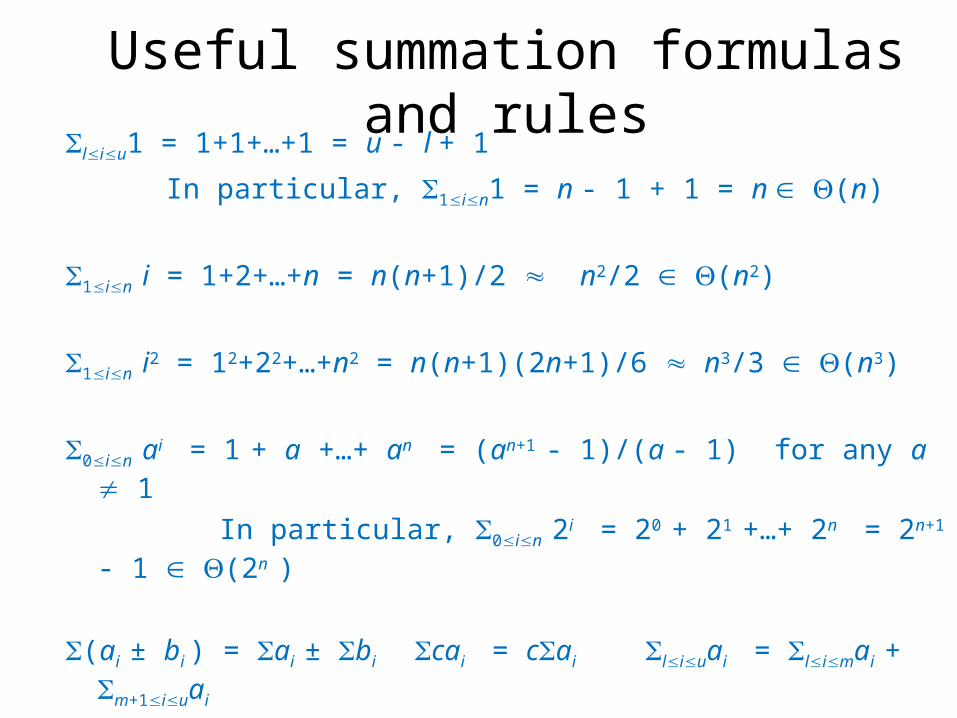
Useful summation formulas and rulesliu1 = 1+1+…+1 = u - l + 1
In particular, 1in1 = n - 1 + 1 = n (n)
1in i = 1+2+…+n = n(n+1)/2 n2/2 (n2)
1in i2 = 12+22+…+n2 = n(n+1)(2n+1)/6 n3/3 (n3)
0in ai = 1 + a +…+ an = (an+1 - 1)/(a - 1) for any a 1
In particular, 0in 2i = 20 + 21 +…+ 2n = 2n+1 - 1 (2n )
(ai ± bi ) = ai ± bi cai = cai liuai = limai + m+1iuai
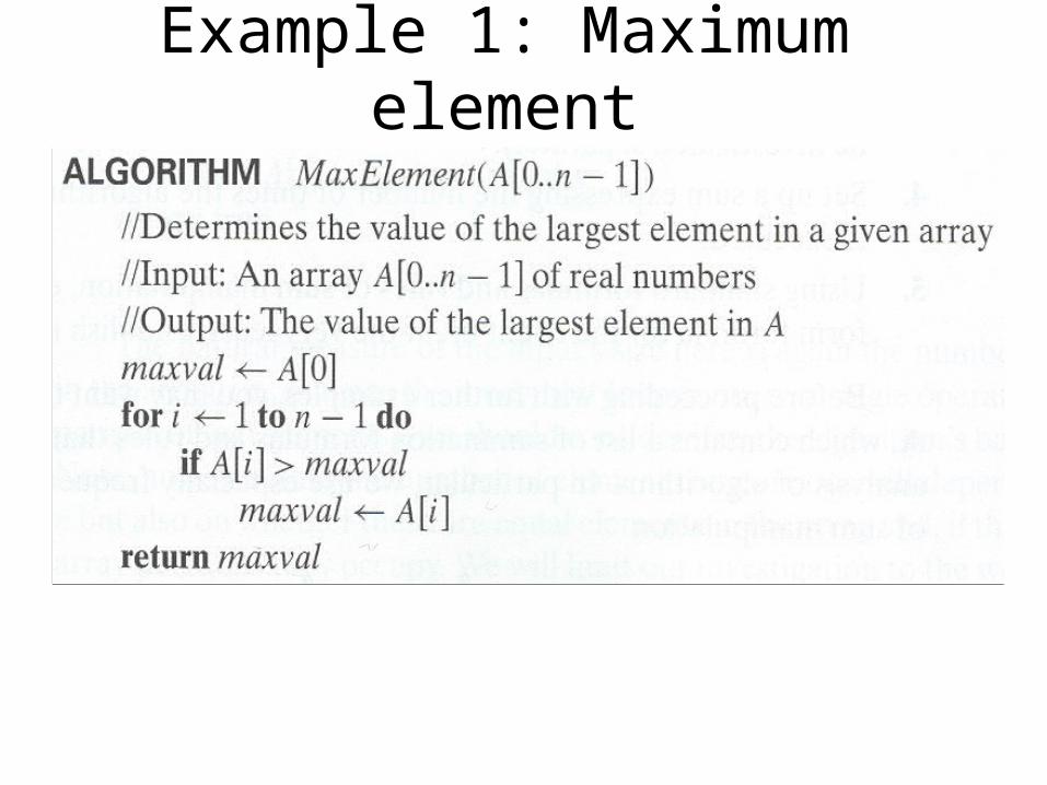
Example 1: Maximum element
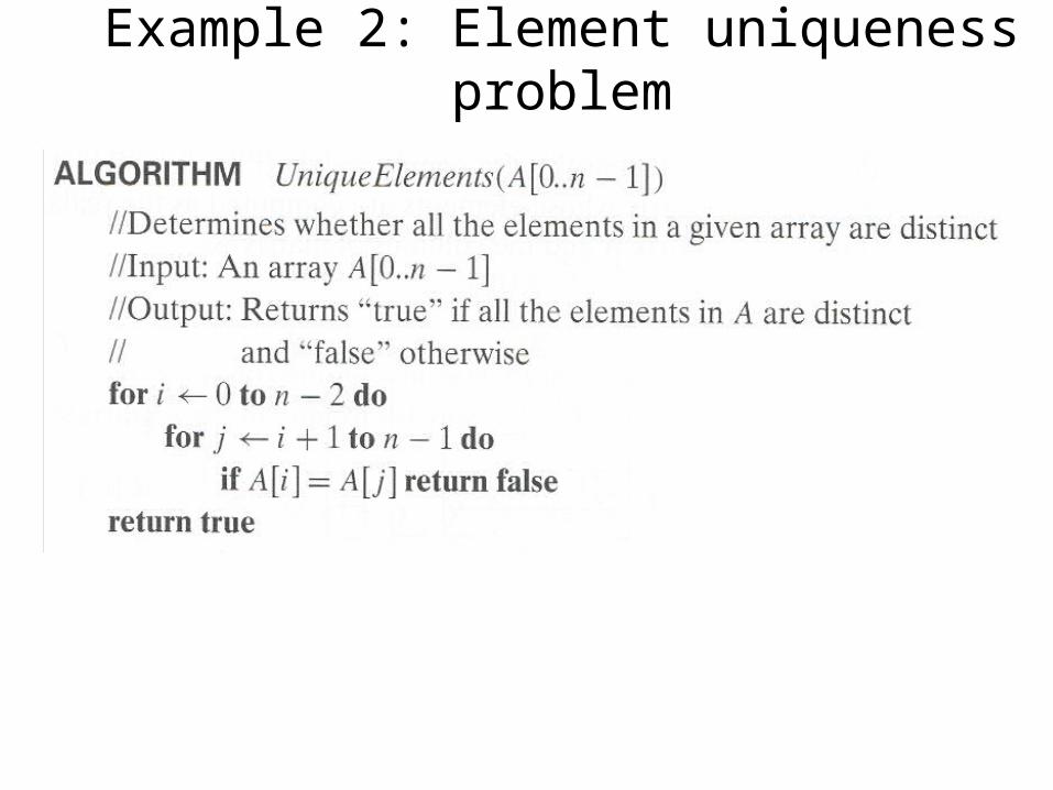
Example 2: Element uniqueness problem
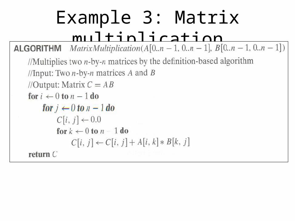
Example 3: Matrix multiplication
Plan for Analysis of Recursive Algorithms
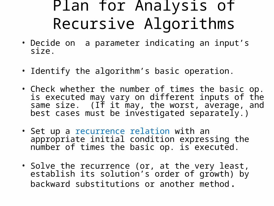
• Decide on a parameter indicating an input’s size.
• Identify the algorithm’s basic operation.
• Check whether the number of times the basic op. is executed may vary on different inputs of the same size. (If it may, the worst, average, and best cases must be investigated separately.)
• Set up a recurrence relation with an appropriate initial condition expressing the number of times the basic op. is executed.
• Solve the recurrence (or, at the very least, establish its solution’s order of growth) by backward substitutions or another method.
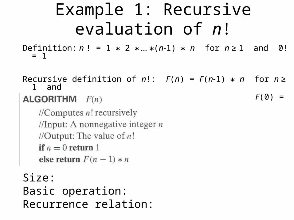
Example 1: Recursive evaluation of n!
Definition: n ! = 1 2 … (n-1) n for n ≥ 1 and 0! = 1
Recursive definition of n!: F(n) = F(n-1) n for n ≥ 1 and F(0) = 1
Size:Basic operation:Recurrence relation:
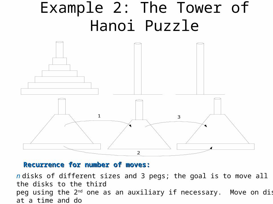
Example 2: The Tower of Hanoi Puzzle
1
2
3
Recurrence for number of moves:Recurrence for number of moves:
n disks of different sizes and 3 pegs; the goal is to move all the disks to the third peg using the 2nd one as an auxiliary if necessary. Move on disk at a time and donot place a larger disk on top of a smaller one!
The Tower of Hanoi Puzzle
• T(n) = 2T(n-1) + 1• T(1) = 1
Example 3: Binary Search
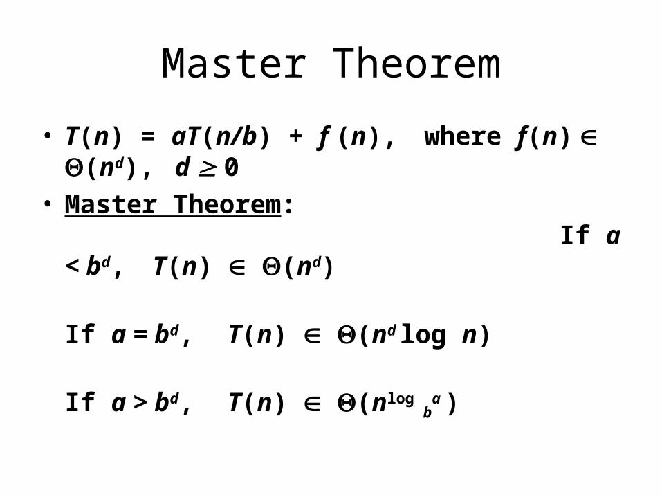
Master Theorem
• T(n) = aT(n/b) + f (n), where f(n) (nd), d 0• Master Theorem:
If a < bd, T(n) (nd) If a = bd, T(n) (nd log n) If a > bd, T(n) (nlog
ba )
Recommended