An Overview of Population Models of Epidemics
April 2020
2
Copyright © 2020 Society of Actuaries
An Overview of Population Models of Epidemics AUTHOR
Patrick Wiese, ASA
Lead Modeling Research Actuary
Society of Actuaries
REVIEWERS
Mary Pat Campbell, FSA, MAAA, PRM
Rowland Davis, FSA
R. Dale Hall, FSA, MAAA, CERA, CFA
Nilesh Mehta, FSA, MAAA
Max J. Rudolph, FSA, CFA, CERA
Drew Slimmer
Martin Snow, FSA, MAAA
Lane B. West, FSA, MAAA, EA
The author’s deepest gratitude goes to the volunteers who generously shared their wisdom, insights, advice, guidance, and arm’s-length review of this study prior to publication. Any opinions expressed may not reflect their opinions nor those of their employers. Any errors belong to the author alone.

3
Copyright © 2020 Society of Actuaries
TABLE OF CONTENTS
1. Importance of Modeling Epidemics ....................................................................................................................... 4
2. The Challenges of Modeling an Outbreak Caused by a Novel Pathogen ................................................................. 5
3. Three Phases of Outbreak Modeling ...................................................................................................................... 8
4. Key Terms that Describe Virus Transmission and Virulence ................................................................................... 8
5. Overview of Approaches for Projecting Outbreaks Forward in Time .................................................................... 10
6. Outbreak Simulations Using a Stylized SIR Model ................................................................................................ 11
7. Communicating Forecast Results, and the Importance of Sensitivity Testing ....................................................... 16
8. Updating Models of Epidemics ............................................................................................................................ 18
9. Economic Costs and Benefits of Outbreak Interventions ...................................................................................... 18
10. Conclusions ....................................................................................................................................................... 19
About The Society of Actuaries ................................................................................................................................ 20
4
Copyright © 2020 Society of Actuaries
1. Importance of Modeling Epidemics
The 1918 flu pandemic, often referred to as the “Spanish Flu”, infected an estimated 500 million persons and
resulted in at least 50 million deaths, equivalent to about 3% of the world’s population at that time.1 While there
have been major advances in medicine over the last 100 years, and vaccines have reduced the risk of outbreaks of
transmissible diseases, the 1918 pandemic serves as a reminder that a novel pathogen can rapidly infect a large
percentage of the human population over a short time period, with devasting consequences.
New virus strains arise on a regular basis through mutation. In addition, a virus that previously existed only in animal
hosts may jump to the human population. The jump could be facilitated by a mutation that increases the capacity of
the virus to enter human cells, or via the merger or “recombination” of genetic material from two separate viruses
that, by chance, simultaneously infect a single animal cell, leading to the creation of an entirely new virus.2
A new virus that finds its way into the human population holds a temporary competitive advantage: its novel
structure makes it less likely to encounter a strong immune defense. Few people may possess immunity to the virus,
or perhaps none at all. Meeting little or no resistance, a new virus has the potential to spread rapidly, causing an
epidemic or pandemic.3
In the event of an outbreak, simulation models can provide policymakers, governments and citizens with a means to
assess strategic options. One course of action is to do nothing, letting the outbreak run its natural course. If
simulations indicate that this could lead to unacceptably high loss of life, additional simulations can be run to
evaluate the impact of actions intended to decelerate or halt the outbreak. Models can provide a rough sense of the
effect of options such as school closures, closures of bars and restaurants, travel restrictions, and stay-at-home or
shelter-in-place orders. For each option, a forecast of the daily demand for hospital services can be compared
against hospital capacity, the goal being to avoid a scenario in which hospitals are overwhelmed with an abrupt
surge in the number of new patients.
When forecasting an outbreak caused by a novel pathogen, model builders must contend with many unknowns. The
speed of an outbreak may leave the scientific community scrambling to collect and analyze data needed to
understand the pathogen’s risk characteristics. Data limitations compel modelers to use assumptions that may have
a wide range of uncertainty, and, as a consequence, outbreak forecasts also have a wide range of uncertainty. A
particular forecast could, for example, indicate that anywhere from 0.3% to 1.0% of a region’s population could die
in the absence of interventions to slow the spread of an infection. A wide range of predicted outcomes may
frustrate policymakers and citizens who seek a more precise quantification of risk. However, a range of predicted
outcomes is preferable to the alternative of “flying blind”, without any guidance and insight from data-driven
forecasts. Without forecasts, the human race could be caught completely off-guard, deprived of the opportunity to
reshape its fate via timely interventions.
Thus, the primary purpose of epidemic projection models is to guide public policy decisions. Outbreak models help
policy makers evaluate the risk posed by an uncontrolled epidemic, and compare the relative outcomes of various
actions intended to alter the epidemic’s trajectory.
1 https://www.npr.org/2020/04/02/826358104/the-1918-flu-pandemic-was-brutal-killing-as-many-as-100-million-people-worldwide 2 An overview of virus mutation is available here: https://www.ncbi.nlm.nih.gov/books/NBK8439/. An overview of how viruses can jump from one species to another is available here: https://www.ncbi.nlm.nih.gov/pmc/articles/PMC2546865/ 3 https://www.dictionary.com/e/epidemic-vs-pandemic/
5
Copyright © 2020 Society of Actuaries
2. The Challenges of Modeling an Outbreak Caused by a Novel Pathogen
For an outbreak caused by a novel pathogen, the starting point for researchers is usually a small dataset – perhaps
gathered from a single city or region – which is likely to fall short of what is needed to provide confident answers to
the following key questions:
• How easily or rapidly is the virus transmitted, and under what conditions?
• What is the average length of the infectious period, and how does this period vary from one individual to
another?
• How long can the virus survive outside of a human host (for example, on a kitchen counter)?
• What is the risk of death for those who are infected?
• What factors influence the risk of death, such as age, gender, race, economic status and comorbidities?
• Are there individuals who have been infected but who exhibit no symptoms, or whose symptoms are so mild
that they don’t need to visit a doctor?
• Is immunity acquired by those who survive an infection?
• If infection does convey immunity, how long does that immunity last? Indefinitely? Or for a finite period?
• Are there country, region and city-specific factors that influence the rate of transmission and/or the fatality
rate?4
• Does weather influence the transmission rate? For example, is transmission correlated with temperature or
humidity levels?
The passage of time gradually increases the body of evidence available to researchers, and, eventually, reliable
answers to these questions can generally be provided. But when faced with an outbreak that is rapidly progressing,
time is a luxury that decision-makers do not have. In the early stages of an outbreak, a virus may spread at a
geometric rate (Table 1), leaving little time for model builders to gather data and refine their forecasts.
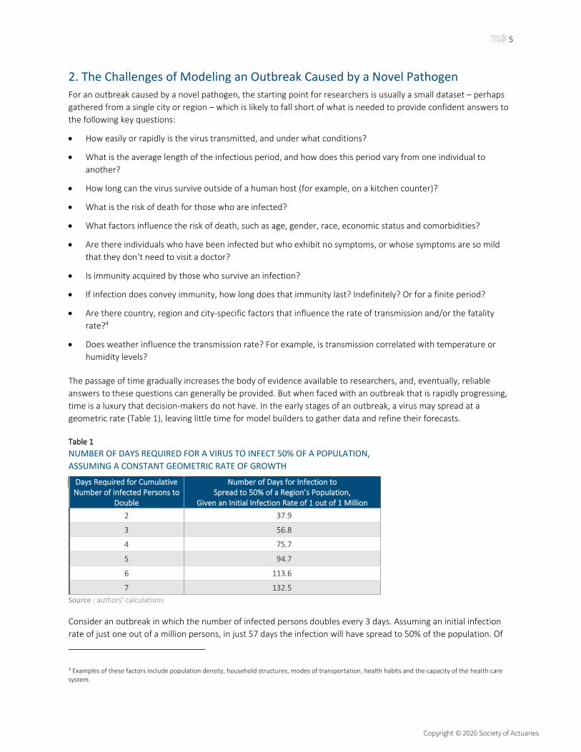
Table 1
NUMBER OF DAYS REQUIRED FOR A VIRUS TO INFECT 50% OF A POPULATION,
ASSUMING A CONSTANT GEOMETRIC RATE OF GROWTH
Days Required for Cumulative Number of Infected Persons to
Double
Number of Days for Infection to Spread to 50% of a Region’s Population,
Given an Initial Infection Rate of 1 out of 1 Million
2 37.9
3 56.8
4 75.7
5 94.7
6 113.6
7 132.5
Source : authors’ calculations
Consider an outbreak in which the number of infected persons doubles every 3 days. Assuming an initial infection
rate of just one out of a million persons, in just 57 days the infection will have spread to 50% of the population. Of
4 Examples of these factors include population density, household structures, modes of transportation, health habits and the capacity of the health care system.

6
Copyright © 2020 Society of Actuaries
course, geometric growth cannot continue indefinitely due to the finite size of a population, and an outbreak
naturally decelerates after a large percentage of a population has been exposed. Nevertheless, the results in Table 1
roughly illustrate the severe time constraints under which model builders and decision-makers must operate.
With respect to SARS-CoV-2 – the coronavirus that causes the illness known as COVID-19 – data from Johns Hopkins
University indicates that, in many countries, the rate of growth of reported cases was rapid during the early stages
of the outbreak (Table 2). In the United States and Italy, for example, the total number of cases doubled from 1 per
100 thousand to 2 per 100 thousand persons in just 2.4 days. In the United Kingdom, Canada and France, this
increase occurred in about 3.2 days.
Table 2
DOUBLING TIME FOR TOTAL REPORTED COVID-19 CASES,
AFTER FIRST REACHING A THRESHOLD OF ONE CASE PER 100,000 OF GENERAL POPULATION
Country Date on Which Cumulative
Cases First Exceeded One Per 100,000 Persons
Number of Days for Reported Cases to Double to
Two Per 100,000 Persons
Iran Mar-01 1.6
Spain Mar-07 1.8
Italy Feb-27 2.4
US Mar-15 2.4
Korea, South Feb-23 2.8
United Kingdom Mar-13 3.1
France Mar-06 3.2
Canada Mar-16 3.2
Russia Mar-29 3.4
Germany Mar-08 4.0
China Feb-02 4.8
Source : author’s calculations using Johns Hopkins University’s COVID-19 database5
Thus, outbreak modelers operate under extreme time pressure, and with much at stake. Delaying a model’s release
by a month to refine its key parameters could render it useless to decision-makers. Model forecasts are most
valuable to decision-makers early in an outbreak. In general, the earlier an intervention such as social distancing is
implemented, the greater will be its likely impact.
Time pressure forces outbreak modelers to make do with the limited data that is available early in an outbreak, and
the data’s limitations make it difficult to assess the threat posed by a novel virus. Recent history provides some
sense of the magnitude of this challenge. In the spring of 2009, a novel influenza virus emerged and spread rapidly
throughout the world. Referred to as “Swine Flu”, researchers scrambled to process emerging data and develop
estimates of the danger posed by this virus. In a report published in 2013, four years after the outbreak, the
National Institutes of Health (NIH) reviewed 77 estimates of Swine Flu case fatality risk from 50 published studies.6
Many of the 77 estimates were produced in the first nine months of the pandemic. The NIH found “substantial
heterogeneity in the published estimates, ranging from less than 1 to more than 10,000 deaths per 100,000 cases or
5 https://github.com/CSSEGISandData/COVID-19/tree/master/csse_covid_19_data/csse_covid_19_time_series 6 Wong, Jessica Y., et al. (2013, November 24). “Case Fatality Risk of Influenza A(H1N1pdm09): A Systematic Review.” Epidemiology (Cambridge, Mass.), 24(6), 830–841. https://www.ncbi.nlm.nih.gov/pmc/articles/PMC3809029/.

7
Copyright © 2020 Society of Actuaries
infections.” The report concludes that “our review highlights the difficulty in estimating the seriousness of infection
with a novel influenza virus”.7
If humans were clones of each other – with identical levels of health, identical immune systems and an identical
chance of succumbing to any particular virus – and if all cities (or regions) were copies of each other, with identical
mobility patterns, identical household structures, identical patterns of social contact and identical health care
systems – the task of quantifying the risk posed by a new virus would be far easier. In this simplified world, a virus
that claimed the lives of 0.5% of the population in city “A” would be likely to have the same effect in city “B”.
Correspondingly, if closing schools in city “A” reduced the fatality rate from 0.5% to 0.2%, then a similar effect could
be expected in city “B”.
Obviously, this “clone” world is not the real world, where individuals differ greatly with respect to health status,
immune response, and social behavior, and where cities and regions vary with respect to population density, age
distribution, household structures, mobility patterns, weather and health care services. These differences can
impact both the rate of virus transmission as well as the risk a virus poses to those who become infected.
Thus, outbreak modelers must contend with the possibility that data gathered from region “A” may not be directly
applicable to region “B”. To some extent, it may be possible to address this issue. For example, if virus transmission
and/or lethality are correlated with age, then differences in age distributions between region “A” and “B” can be
factored into forecasts. However, in the early stages of an outbreak, many key factors that affect virus transmission
and lethality may go undetected. Suppose, for example, that air pollutants influence the transmission of a particular
virus, but the initial data is drawn solely from one city. Without data collected from a range of cities with varying air
quality, researchers may lack the covariates required to statistically link air pollutants to virus transmission.
Even in the absence of differences between region “A” and “B”, modelers must contend with the problem of sample
bias. As with any statistical analysis, a biased sample may produce a distorted set of conclusions that are not
applicable to the population as a whole. A common source of sample bias in an outbreak arises as follows: some
individuals become very sick and must be hospitalized, and these individuals are captured in the data; in contrast,
other individuals experience mild symptoms or perhaps no symptoms whatsoever, and these individuals are not
captured in the data. Thus, the data includes only those individuals who were severely affected by the virus, and, as
a consequence, fatality rates estimated from the data will overstate the risk posed to the general population.
In addition, even if a sample is unbiased, it may lack the size required to develop narrow confidence intervals for key
parameters. For the sake of argument, suppose that all individuals are identical clones, sharing the same health
status and immune response, and with the same probability of succumbing to any particular virus. Consider a cruise
ship with 500 “clone” passengers. Suppose that all passengers become infected by a virus, and that 2% die. Even in
this simple case, substantial uncertainty exists regarding the fatality rate. Assuming that the outcome for each
individual is an independent Bernoulli trial8, and using the Central Limit Theorem9 to infer that the sum of
independent Bernoulli trials is an approximately normal distribution, the 90% confidence interval for the case
fatality rate is quite wide, running from 0.97% to 3.03%.
Lastly, modelers must contend with data reporting methods that may vary from country to country, region and
region, and city to city. For example, a particular locality may require a positive laboratory test (for a particular type
of virus) before entering a case into its database. Other localities may rely on the judgment of a patient’s doctor (or
7 With the passage of time and the expansion of available data, researchers were able to produce increasingly reliable estimates of the mortality risk posed by (H1N1)pdm09, the virus that caused the Swine Flu outbreak of 2009. Today, more than ten years after the outbreak, the Centers for Disease Control and Prevention (CDC) estimates that 61 million Americans were infected with the virus during the one-year period beginning in April 2009, of which 12.5 thousand persons died. This translates into an infection mortality rate of 0.02%. This is less than the CDC’s estimate of 0.1% for the mortality rate associated with seasonal flu. 8 https://www.sciencedirect.com/topics/mathematics/bernoulli-trial 9 https://mathworld.wolfram.com/CentralLimitTheorem.html
8
Copyright © 2020 Society of Actuaries
coroner) to assess whether an individual is (or was) infected. Even if laboratory tests are used as opposed to human
judgment, the tests may not yet be 100% reliable (because the pathogen is novel), producing false positive and false
negative results. Moreover, if a patient with poor health status dies from a virus, it may be unclear whether the virus
was the primary cause of death, or if the patient would have died anyway from another condition.
3. Three Phases of Outbreak Modeling
Roughly speaking, an outbreak can be divided into three main phases – (1) the start, (2) the early stages, and (3) the
latter stages – each of which poses unique challenges and goals for outbreak modelers.
Phase 1 consists of the start of an outbreak. The primary modeling goal is to quickly assess whether the health risks
are so great that significant mitigation efforts are needed, and to estimate the impact of various mitigation
responses. Simulation results have a global and country-level granularity. The range of projected outcomes will be
very wide because of great uncertainty associated with key input parameters. Worst case results take a prominent
role, as policy makers need to consider actions that "insure" against the worst case until more certainty emerges as
the outbreak progresses.
Phase 2 corresponds to the early stages of the outbreak. Here the modeling focus shifts to specific regions, with an
emphasis placed upon determining if localities have sufficient medical resources to meet expected demand. In
addition, the pool of available data widens, allowing modelers to update their initial assumptions and refine their
forecasts.
Phase 3 begins as the outbreak decelerates, with declines in the number of emerging cases. Modelers focus on
estimating the effects of relaxing mitigation efforts. This is similar to phase 1 modeling work, but with somewhat
better input certainty and a more regional focus.
4. Key Terms that Describe Virus Transmission and Virulence
Outbreak modelers and epidemiologists use various terms and statistics to describe the risk posed by a virus. Key
terms are as follows:
Basic reproduction number (R0)
The average number of persons to whom an infected person transmits the virus, assuming that all individuals in a
population are susceptible to infection. This value is often referred to as “R0” or “R naught”. A value of 2, for
example, indicates that, on average, an infected person will transmit the virus to two additional persons. R0 depends
not only on the characteristics of a virus, but also upon social and environmental factors. Thus, a particular virus
might have an R0 of 2.5 when estimated for a dense urban area, but only 1.8 when measured in a rural area.
All else being equal, the larger the value of R0, the greater will be the speed of an outbreak. But R0 by itself does not
provide a measurement of the rate at which an outbreak spreads. For example, both a slowly evolving outbreak and
a quickly evolving outbreak could have an R0 of 2.0. In the slow outbreak, an individual’s infectious period would be
relatively long, but the risk of transmission on any particular day of that period would be relatively low. In the fast
outbreak, the infectious period would be shorter, but the risk of transmission on any particular day would be larger.
If R0 is less than 1.0, the number of new infections will decline across time. Conversely, if R0 is greater than 1.0, then
an infection could, in theory, spread throughout a population. In general, the greater the value of R0, the harder it
will be to control an outbreak.

9
Copyright © 2020 Society of Actuaries
Effective reproduction number (Re)
The average number of persons to whom an infected person transmits the virus, given the current state of the
population, and including the effects of any mitigation efforts. At the outset of an outbreak caused by a novel
pathogen, the entire population is usually considered susceptible, and governments haven’t yet had time to take
actions to mitigate virus transmission. Consequently, R0 and Re are identical. As an outbreak progresses, the
susceptible population declines, assuming that immunity is conferred upon those who survive the infection. All else
being equal, if the recovered population is 50% of the total population, then Re will be half of R0. Actions to reduce
virus transmission – such as social distancing – can lead to further reductions of Re. Thus, Re is a dynamic value that
changes across time in response to declines in the susceptible population and efforts to mitigate virus transmission. Incubation period
The period between an individual’s exposure to a virus and the onset of clinical symptoms.
Infectious period
The period during which an infected individual can transmit the virus to another person. Depending on the virus and
to some extent the individual, the infectious period may begin immediately after infection, or there may be a lag
between the time of infection and the time at which the individual becomes infectious. For some viruses, the
infectious period may overlap with the incubation period, while for other viruses there may be no overlap.
Generation time
If a person transmits a virus to another person, the time between the onset of symptoms in the first person and the
onset of symptoms in the second person is referred to as “generation time”. In general, the shorter the average
generation time and the larger the basic reproduction number, the greater the speed with which an infection
propagates through a population. Case Fatality Rate (CFR)
The number of virus-related deaths divided by the number of diagnosed cases. Ideally, a CFR should be calculated
using cases that have already reached a conclusion (i.e. recovery or death). In the early stages of an outbreak,
however, it may be difficult to determine how many reported cases have reached a conclusion. It may be necessary,
therefore, to impute the number of completed cases as a function of the number of reported cases.
Note that the CFR may be affected by sample bias: in the early stages of an outbreak, the CFR typically captures only
the most severe cases, and thus may fail to be a good indicator of the risk posed to the population that is not yet
infected.
A CFR is not identical to a mortality rate. A mortality rate is typically expressed as an annual rate, while a CFR is
independent of time. For example, consider a fast-acting virus that runs its course in merely one week, resulting in
death in 10% of cases. This virus has the same CFR as a virus that kills 10% of infected persons, but does so across an
average period of illness of 12 months.
Hospitalization Fatality Rate (HFR)
This is similar to the CFR, but is focused solely on those individuals who were hospitalized. For a particular region,
the HFR will generally be greater than the corresponding CFR. The CFR typically captures at least some individuals
with mild to moderate symptoms, while the HFR tends to capture only those individuals with severe symptoms.
These sample biases, in turn, push the HFR upwards relative to the CFR.
Infection Fatality Rate (IFR)
Like the CFR and HFR, the IFR is equal to deaths divided by cases. But the IFR captures not only all diagnosed cases,
but also mild and “subclinical” cases that do not typically lead to visits to a physician. Thus, an IFR is lower than the
corresponding CFR and HFR.

10
Copyright © 2020 Society of Actuaries
5. Overview of Approaches for Projecting Outbreaks Forward in Time
Roughly speaking, there are two main types of outbreak forecasting models: 1) statistical models and (2)
mechanistic models. The Institute for Health Metrics and Evaluation (IHME) COVID-19 model10, which has been
frequently cited by the media as well as by the White House11, is an example of a statistical model12, while the
Imperial College of London’s COVID-19 model13,14 is an example of a susceptible-infected-recovered (SIR) model,
which is a type of mechanistic model.
A statistical model uses correlations or patterns in data to forecast the propagation of a virus. A common approach
is to focus on the time series of virus-related deaths, separately by city or geographic region, fitting this data to a
curve that describes the anticipated rise, peak and fall of the number of daily deaths. The curve might be extracted
from cities or regions that have already passed through the outbreak (such as Wuhan, China, with respect to COVID-
19). The assumption is that, in each different region, the outbreak will follow a similar “shape”, curve or pattern
across time. A model may tweak or adjust the assumed outbreak shape to account for region or city-specific factors,
such as delays associated with implementing social distancing measures.
In contrast to statistical models, mechanistic models focus on the dynamic processes by which a virus propagates
through a population. Estimates of the transmissibility and lethality of the virus are used to simulate the progression
of an outbreak across time. A SIR model, for example, projects shifts in the population from “susceptible” (i.e. not
yet infected) to “infected”, and from “infected” to either “recovered” or deceased. Some SIR models are quite
simple in that they assume that all persons have an equal chance of becoming sick, that infected persons are equally
likely to transmit the virus, and that infected persons share the same probability of death. More complicated SIR
models subdivide the population into groups, each group having distinct characteristics with respect to risk of
infection, risk of transmission, and risk of death. Some SIR models go a step further, using an agent-based method to
simulate unique individuals (as opposed to groups of individuals), each interacting with other unique simulated
individuals.
Complex mechanistic models with multiple subgroups demand more data and assumptions relative to simple
models that assume a homogenous population, but their higher level of detail can be helpful to policy makers who
seek an efficient approach to reduce virus transmission while minimizing disruptions to the economy and to the lives
of citizens. For example, a multi-subgroup model could allow policy makers to study the effects of focusing social
distancing on high-risk subgroups, while using a more relaxed approach for low-risk subgroups. Additionally,
modelers may wish to create a subgroup specifically for health care workers because a deterioration in their health
status could reduce a health care system’s capacity to serve patients, which, in turn, could have a negative effect
across all modeled subgroups.
Model subgroups can be used not only to represent different levels of risk, but also to capture social relationships
that could influence virus transmission. For example, models may differentiate between students, workers and
retirees, with assumptions describing the rates of social contact both within and across these groups. In general, the
greater the number of subgroups, the greater the capacity of a model to capture the complex web of social
10 Murray, Christopher JL. (2020, March 30). “Forecasting COVID-19 Impact on Hospital Bed-Days, ICU-Days, Ventilator-Days and Deaths by U.S. State in the Next Four Months.” MedRxiv. https://www.medrxiv.org/content/10.1101/2020.03.27.20043752v1. 11 Aizenman, Nurith. (2020, April 1). “Five Key Facts Not Explained in White House COVID-19 Projections.” NPR. https://www.npr.org/sections/health-shots/2020/04/01/824744490/5-key-facts-the-white-house-isnt-saying-about-their-covid-19-projections. 12 While the IHME model uses a statistical approach to project the number of deaths, the component of the model that projects hospital service utilization is best described as mechanistic. Thus, the IHME model has both statistical and mechanistic components. 13 Flaxman, Seth, et al. (2020, March 30). “Report 13—Estimating the Number of Infections and the Impact of Non-Pharmaceutical Interventions on COVID-19 in 11 European Countries.” Imperial College London. https://www.imperial.ac.uk/mrc-global-infectious-disease-analysis/covid-19/report-13-europe-npi-impact/. 14 Adam, David. (2020, April 2). “Special Report: The Simulations Driving the World’s Response to COVID-19.” Nature. https://www.nature.com/articles/d41586-020-01003-6.
11
Copyright © 2020 Society of Actuaries
relationships that tie individuals together into a society. Greater realism, in turn, can improve a model’s ability to
estimate the impact of interventions aimed at decelerating an outbreak.
A multi-subgroup model that is calibrated to one region may not be well suited to another region, unless
adjustments are first implemented to reflect the region-specific social conditions that can affect the number and
type of social contacts. This is especially true if an epidemic disproportionately impacts one segment of society, such
as the elderly, whose social interactions differ across countries or regions. For example, consider a region “A” with
relatively large households that often include both retirees and people of working age, compared to a region “B”
with smaller households that rarely include both retirees and people of working age. Clearly, a model parameterized
to reflect the social relationships of region “A” would not be optimal for region “B”. Of course, if parameters are
flexible, it may be possible to recalibrate the model to reflect region-specific social structures.
There is no simple rule-of-thumb for determining which modeling approach – statistical or mechanistic – is best for
modeling a particular outbreak. One consideration is the availability and reliability of various types of data. Statistical
models do not require estimates of parameters that describe virus transmission and virulence, such as the basic
reproduction number, mean generation time and the case fatality rate. Nor do they require data that describes the
social structures that can influence virus transmission. Instead, statistical models use data that describes the effects
(rather than the causes) of an outbreak, such as data for reported deaths. By focusing directly on outbreak effects
(i.e. deaths), some might argue that a statistical approach minimizes a model’s dependency on uncertain parameter
estimates. However, regardless of modeling approach, it is not possible to sidestep the issue of uncertainty. In a
statistical model, uncertainty arises because statistical patterns observed in data may not be predictive of the
future, and may not be widely applicable across different countries, regions and cities.
With respect to modeling outbreak mitigation options, it is arguable that mechanistic models hold an advantage
relative to statistical models. Consider a complex strategy in which initial social distancing policies are gradually
phased down across time, but will be reintroduced in the event that new cases rise above a critical threshold. This
strategy could potentially lead to a series of peaks and troughs of new cases. A statistical model that is geared
towards estimating a single outbreak wave might require considerable adjustments to simulate this mitigation
strategy. A mechanistic model, in contrast, may require little alteration, since it focuses on the underlying dynamics
of disease propagation.
6. Outbreak Simulations Using a Stylized SIR Model
Perhaps the most common approach for forecasting an outbreak is to divide a simulated population into
compartments that represent illness progression, and to estimate the movement, across time, of individuals
between these compartments. Not surprisingly, these models are referred to as “compartmental” models. They fall
into the “mechanistic” model class described earlier in the paper. Compartmental models may also be referred to as
“population” models or “metapopulation” models. Compartmental models may be either deterministic or
stochastic, and they may operate either in discrete or continuous time.
One type of compartmental model is a “SIR” model. As described earlier in this paper, “SIR” stands for “susceptible,
infected and recovered”. Sometimes the term “removed” is used as opposed to “recovered”. A SIR model assumes
that immunity is conferred to survivors of an infection. Once infected, an individual cannot become infected a
second time, and they are “removed” from the simulation. Thus, the flow between compartments in a SIR model is
unidirectional: the simulated population gradually shifts from susceptible to infected, and from infected to removed
(i.e. deceased or recovered).
The SOA has developed a stylized SIR model for illustrative purposes. The model is not intended to simulate an
actual outbreak associated with a real virus, but rather to illustrate basic concepts of compartmental models of

12
Copyright © 2020 Society of Actuaries
epidemics. None of the simple illustrations generated by this model are a basis for a government or a policy maker
to pursue a particular course of action, and none of the exhibits presented in the example that follows should be
viewed as a statement of actuarial opinion. Rather, the goal is merely to offer an overview of how a basic SIR model
operates.
The SOA model operates in discrete time, projecting forward in one-day steps. The projected population state on
day “N” is a deterministic function of the projected state on day “N - 1”. A user specifies the population state at time
zero by entering the fraction of the total population that is initially infected (e.g., 1 out of 100 thousand persons).
The remainder of the population is placed into the “susceptible” compartment, indicating that they are at risk of
contracting the infection.
The SOA model can simulate a homogenous population in which all individuals share the same risk of contracting an
infection and the same risk of dying from an infection. Alternatively, the population can be categorized into two
groups, each of which is assigned its own risk characteristics. The model assumes that these two groups coexist with
each other and mix freely together, such that transmission can occur across groups.
Virus transmission is modeled with three parameters: (1) the probability of transmission if an infected person comes
into contact with an uninfected person, (2) the average number of person-to-person contacts each day, and (3) the
average duration of an infection. The product of these three values is the basic reproduction number (R0), as shown
in Table 3.
Table 3
EXAMPLE OF VIRUS TRANSMISSION PARAMETERS FOR THE SOA’S ILLUSTRATIVE SIR MODEL
Parameter Value
Transmission probability if infected person comes into contact with uninfected person 1%
Number of social contacts per person each day 50
Average duration of infection, in days 5
R0 = transmission probability * daily social contacts * duration of infection 2.5
The SOA model simulates social distancing by providing the flexibility to vary the person-to-person contact
parameter. The parameter can be set at an initial “no distancing” level, and, at a user-specified point in the
simulation, can be dropped to a lower “with distancing” level. “With distancing” can be kept in place until the end of
the simulation, or, alternatively, the model can revert back to “no distancing” after a user-specified time period.
To project forward from day “N - 1” to “N”, the SOA model uses the following equations, where “S”, “I” and “R”
represent “susceptible”, “infected” and “recovered”, respectively, each expressed as a percent of the total
population:
Newly Removed = IN-1 / Average Duration of Infection
New Deaths = Newly Removed * Infection Fatality Rate
Newly Infected = SN-1 * [IN-1 – Newly Removed] * Daily Contacts * Transmission Probability per Contact
SN = SN-1 – Newly Infected
IN = IN-1 – Newly Removed + Newly Infected
RN = RN-1 + Newly Removed
Note that SN + IN + RN = 100%
13
Copyright © 2020 Society of Actuaries
For the sake of simplicity, new removals and new infections are not assumed to occur simultaneously. Rather, new
removals are calculated first, followed by new infections. This simplifying assumption is reasonable in a stylized
model, but a real model would typically use an approach with greater mathematical precision.
The rate of new infections is proportional to the product of “S” and “I” (the susceptible and infected populations,
respectively). This product will grow during the early stages of the simulation of an uncontrolled outbreak,
eventually reaching a maximum that roughly corresponds to the peak of the outbreak. Thereafter, the product will
decline, and, ultimately, will drop to zero (or close to zero). Rather like a wildfire burning through a forest,
eventually the fuel – in the form of persons who have not yet caught the virus – will be exhausted or greatly
diminished, thus bringing the outbreak to a conclusion.
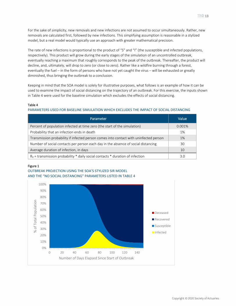
Keeping in mind that the SOA model is solely for illustrative purposes, what follows is an example of how it can be
used to examine the impact of social distancing on the trajectory of an outbreak. For this exercise, the inputs shown
in Table 4 were used for the baseline simulation which excludes the effects of social distancing.
Table 4
PARAMETERS USED FOR BASELINE SIMULATION WHICH EXCLUDES THE IMPACT OF SOCIAL DISTANCING
Parameter Value
Percent of population infected at time zero (the start of the simulation) 0.001%
Probability that an infection ends in death 1%
Transmission probability if infected person comes into contact with uninfected person 1%
Number of social contacts per person each day in the absence of social distancing 30
Average duration of infection, in days 10
R0 = transmission probability * daily social contacts * duration of infection 3.0
Figure 1
OUTBREAK PROJECTION USING THE SOA’S STYLIZED SIR MODEL
AND THE “NO SOCIAL DISTANCING” PARAMETERS LISTED IN TABLE 4
0%
10%
20%
30%
40%
50%
60%
70%
80%
90%
100%
0 20 40 60 80 100 120 140
% o
f To
tal P
op
ula
tio
n
Number of Days Elapsed Since Start of Outbreak
Deceased
Recovered
Susceptible
Infected

14
Copyright © 2020 Society of Actuaries
Using the inputs from Table 4, the simulated outbreak peaks on day 76, at which point 27% of the population has an
active infection (Figure 1). The daily rate of new infections peaks slightly earlier, on day 69, coinciding with the point
at which the product of the susceptible population and the infected population reaches its maximum. New
infections continue to occur at the end of the 150 day projection horizon shown in Figure 1, but at a very low level
because, at this late stage of the outbreak, the population has developed substantial “herd immunity”.15 By the last
day of the simulation, about 90% of the population has been infected. Of this 90%, 1 out of every 100 died
(reflecting an assumed CFR of 1%), while the remainder survived.
The uncontrolled outbreak shown in Figure 1 has the potential to overrun hospitals. From day 55 through day 106,
at least 5% of the population is infected at any given time. Suppose, for the sake of argument, that 1 out of 10
infected persons require hospitalization. Then between day 55 and day 106, at least 0.5% of the population would
require hospitalization on any given day. This high demand could pose a problem for many health care systems. In
the United States, for example, there are only 2.8 hospital beds per every 1000 persons, and only a small fraction of
these are intensive care beds.16
Therefore, decision-makers may wish to explore options to “flatten the curve”, the goal being to spread new
infections out across time such that hospitals are not overburdened. Social distancing is one option for achieving
this objective. Figure 2 compares the baseline scenario (no social distancing) against two options for social
distancing:
0. No social distancing, which assumes 30 social contacts per person per day.
1. Option “A”: a 90-day period of social distancing, running from day 31 to day 120 of the simulation, during
which time social contacts per person per day are reduced to 15. After day 120, daily social contacts
increase to the baseline level of 30.
2. Option “B”: a 90-day period of social distancing, running from day 51 to day 140 of the simulation, during
which time social contacts per person per day are reduced to 15. After day 140, daily social contacts
increase to the baseline level of 30.
In this example, social distancing temporarily cuts the basic reproduction number (R0) in half, from 3.0 to 1.5. This
slows the transmission of the virus, but does not entirely suppress it. To suppress transmission, R0 must be pushed
down below 1.0.
This example assumes that decision-makers and citizens have an appetite for only 90 days of social distancing. Thus,
the question under consideration is not the length of the social distancing period, but rather when it should be
implemented to maximize its positive impact. Under option A, the period begins on the 31st day of the outbreak,
while under option B, the period begins on the 51st day of the outbreak.
Figure 2 presents projection results, focusing on the number of infected persons as a percent of the population.
Note that this time series was depicted in yellow in Figure 1.
At first glance, the results in Figure 2 are counterintuitive. Option “A” fails to flatten the curve; roughly speaking, it
simply delays the outbreak, with only a slight reduction in the peak relative to the “no distancing” scenario. In
contrast, option “B” has a strong flattening effect despite the fact that social distancing measures were
implemented 20 days later than in option A.
15 Clinical Infectious Diseases, Volume 52, Issue 7, 1 April 2011, Pages 911–916, https://doi.org/10.1093/cid/cir007" 16 https://www.aha.org/statistics/fast-facts-us-hospitals

15
Copyright © 2020 Society of Actuaries
Figure 2
PROJECTED NUMBER OF INFECTED PERSONS USING THE SOA’S STYLIZED SIR MODEL:
NO SOCIAL DISTANCING (SEE PARAMETERS IN TABLE 4) VERSUS TWO SOCIAL DISTANCING OPTIONS
These simulation results raise the following question: how did option B’s implementation delay, relative to option A,
lead to an improvement in the impact of social distancing? In seeking an answer, it is helpful to examine the state of
the projected population at the start and end of the social distancing period:
Table 5
STATE OF PROJECTED POPULATION AT START AND END OF 90-DAY SOCIAL DISTANCING PERIOD
Population “Compartment” Option A Option B
At Start of Social Distancing Period: Susceptible 99.82% 96.10%
At Start of Social Distancing Period: Infected 0.11% 2.43%
At Start of Social Distancing Period: Removed 0.06% 1.47%
At End of Social Distancing Period: Susceptible 92.46% 57.56%
At End of Social Distancing Period: Infected 1.80% 3.12%
At End of Social Distancing Period: Removed 5.74% 39.33%
At End of 300 Day Simulation Period: Removed 91.22% 81.56%
Because neither of the two options results in an R0 below 1.0, the infection persists in the population regardless of
the social distancing policy. After the 90-day social distancing period ends and normal social behavior is restored,
the speed of the outbreak once again accelerates and, eventually, most of the population is exposed to the virus.
This stylized example is analogous to a forest fire that cannot be extinguished, and which will ultimately burn
through most of the forest. The goal is a controlled burn such that only a small portion of the forest is on fire at any
particular point in time, subject to the constraint that firefighters are available only for a total of 90 days.
Under option A, social distancing is implemented at an early stage of the outbreak, when only 0.18% of the
population had been exposed. When social distancing is lifted 90 days later, only about 7.5% of the population has
been exposed, and the remaining 92.5% is susceptible. Thus, most of the “forest” remains, providing the fuel that
eventually leads to a rapid burn and an intense peak.
0%
5%
10%
15%
20%
25%
30%
0 50 100 150 200 250 300
Act
ive
Infe
ctio
ns
as %
of
Tota
l Po
pu
lati
on
Number of Days Elapsed Since Start of Outbreak
NoDistancing
Option A:Day 31 to120
Option B:Day 51 to140
16
Copyright © 2020 Society of Actuaries
Under option B, social distancing is implemented later, when about 4% of the population has been exposed. When
social distancing is lifted 90 days later, over 40% of the population has been exposed, and under 60% is susceptible.
With less remaining “fuel”, the fire then burns at a slower rate relative to option A.
Thus, given a fixed N-day period for social distancing, the outcome is quite sensitive to timing. If the N-day period is
implemented too early, it will do little to flatten the curve; rather, it will simply shift the peak to a later date.
Conversely, waiting too long – until the outbreak is already raging and hospitals are overrun – would defeat the very
purpose of social distancing.
Faced with initial results such as these, a logical next step for a modeler would be to conduct further simulations,
experimenting with a range of social distancing options, thereby developing a broader sense of how projected
outcomes vary as a function of input parameters. For example, it would be instructive to examine simulations in
which social distancing is phased down gradually rather than abruptly. During such an exercise, simulation results
should not be blindly accepted. Rather, a modeler should endeavor to make sense of results, both for each
individual simulation, and across simulations. If results do not match intuition or professional judgment, further
investigation is necessary to ensure that the model is free of defects or programming errors.
At the risk of being repetitive, the purpose of the preceding case study is not to offer specific guidance for policy
makers. Rather, the goal is to provide an overview of a simple SIR model, and to illustrate how such a model can be
used to examine mitigation options.
7. Communicating Forecast Results, and the Importance of Sensitivity Testing
As with any modeling effort, outbreak simulation results need to be clearly presented, along with a description of
the data, methods and key assumptions. Any caveats or concerns about the model should be explained. Given the
high level of uncertainty of key metrics that describe virus transmission and virulence, particularly during the early
stage of an outbreak when data is limited, modelers must reflect the effects of this uncertainty in their forecasts.
Simply providing a most likely scenario would be insufficient because it would convey a false sense of precision and
certainty.
One graphical approach for representing uncertainty is a “cone of uncertainty”, similar to those used in hurricane
forecasts to provide both a most likely storm path as well as range of possibilities around that path.17 The Institute
for Health Metrics and Evaluation (IHME) uses such an approach for visualizing the uncertainty associated with its
online forecast18 for the number of COVID-19 deaths in the United States, as shown in Figure 3. In this case, the
cone of uncertainty represents a 95% confidence interval. The cone reaches a maximum width (rather than
continuing to fan out across time) because the simulation is aimed solely at estimating the “first wave” of the
outbreak, and because the forecast assumes that social distancing measures remain in place until “infections are
minimized and containment is implemented”.
In addition to the graph of the forecast, the IHME’s COVID-19-forecast web page provides a description of the
assumptions, data and methodology used to produce the simulations, and it describes the model’s limitations. For
example, the web page notes the following key limitation: “our model does not yet reflect how easing or lifting
social distancing measures could increase COVID-19 infections and deaths.” Thus, this modeling effort provides a
good example of a clearly communicated forecast.
17 https://www.nhc.noaa.gov/aboutcone.shtml 18 https://covid19.healthdata.org/united-states-of-america

17
Copyright © 2020 Society of Actuaries
Figure 3
IHME’S PROJECTION OF COVID-19 RELATED DEATHS IN THE UNITED STATES, GENERATED ON APRIL 29;
SOCIAL DISTANCING ASSUMED UNTIL INFECTIONS MINIMIZED AND CONTAINMENT IMPLEMENTED
Source : IHME’s COVID-19 projection webpage19, accessed on April 29, 2020
Decision-makers may wish to compare results across models, to assess whether forecasts generated by different
research groups are generally in agreement. This is particularly useful early in an outbreak, when data is limited and
modelers may need to rely heavily on their professional judgment for setting key assumptions.
To facilitate such a cross-model comparison, some researchers focus their efforts on gathering and summarizing
forecasts produced by various models. For example, the Centers for Disease Control and Prevention (CDC) has
created a web page that graphically compares short-term forecasts of deaths due to Covid-19 in the United States:
Figure 4
A COMPARISON OF SHORT-TERM FORCASTS FOR COVID-19 RELATED DEATHS IN THE U.S., COMPILED BY THE CDC
Source : CDC’s COVID-19 projection webpage20, accessed on May 4, 2020
19 https://covid19.healthdata.org/united-states-of-america 20 https://www.cdc.gov/coronavirus/2019-ncov/covid-data/forecasting-us.html

18
Copyright © 2020 Society of Actuaries
The CDC presents the forecast of each of various models, as well as an “ensemble” forecast that, roughly speaking,
is an average forecast computed across models. A brief summary of each model’s methods and assumptions is
provided, along with links to websites associated with each model.
A cross-model forecast summary such as the CDC’s may lead to further questions. For example, decision-makers
may wish to better understand why some models project bleaker outcomes compared to others. Or decision-
makers may wish to determine which model is the “best” or the “most reliable”. These are valid questions, but they
may lack simple answers. Because outbreak modelers must contend both with significant data limitations and the
formidable task of modeling human behavior, there is no single “correct” or “best” modeling approach. Rather,
there are many valid approaches, each involving a range of assumptions that depend, to some extent, on
professional judgment.
8. Updating Models of Epidemics
Outbreak models can quickly become “stale” during the early stages of an outbreak. With little data to draw upon,
initial modeling efforts necessitate the use of assumptions that have a wide range of uncertainty. As an outbreak
progresses, the pool of available data expands, providing researchers with valuable information that can be used to
revise their models.
Inevitably, model revisions result in shifts in outbreak forecasts. Large shifts could potentially undermine the public’s
faith in a model. However, revisions of forecasts do not, in general, arise from a lack of modeling expertise, but
rather from data limitations that are part and parcel of dealing with a new pathogen. Revisions to forecasts are a
sign that modelers are paying attention to the continuous influx of new data produced by researchers around the
world, and diligently adjusting their models to reflect the most current available information about the pathogen.
9. Economic Costs and Benefits of Outbreak Interventions
An outbreak may have significant negative impact on economic activity, and actions to control an outbreak will lead
to economic costs as well as economic benefits. Generally, outbreak models to not attempt to forecast these
impacts on the economy; rather, the models focus on projecting cases, hospitalizations and deaths.
However, policy makers cannot ignore the economic effects of interventions. They weigh the benefits of an
intervention – primarily in the form of lives saved21 – against its impact on health care costs22, unemployment levels,
GDP growth, government expenditures, and the level of government debt. A full examination of the methods used
to project the economic impact of outbreak interventions is beyond the scope of this paper. Nevertheless, it is
useful to briefly consider several outbreak scenarios which can help frame one’s thinking regarding economic costs:
1. A fast-spreading virus with a high IFR: consider a novel virus with an R0 of 4, a mean generation time of just 5
days, and an infection fatality rate (IFR) of 90%. Suppose, for the sake of argument, that researchers have a high
degree of confidence in the estimate of both R0 and the IFR. This is a nightmare scenario involving a fast-
spreading, highly virulent virus that could potentially kill most of the human race over a short time period. In
21 With unlimited resources, decision makers would not have to face the difficult and uncomfortable problem of determining if a particular mitigating action, which could lead to a reduction in expected fatalities, is worth the investment of economic resources. Given that resources are finite, however, this problem is unavoidable. One modeling approach is to estimate the “value of a statistical life” (VSL), which can then be used to translate the estimated number of saved lives (as a result of a mitigating action) into a monetary value. An alternative is to estimate the “value of a statistical life year” (VSLY), which leads to a higher monetary value for saving the lives of younger persons relative to older persons. 22 In a publicly-financed single payor health care system, these costs would be borne by the government. In mixed system, with public and private components, the costs would be distributed across these sectors.
19
Copyright © 2020 Society of Actuaries
this extreme case, the economic calculations become straightforward: any economic cost is justified given that
civilization itself is threatened.
2. A novel virus that will spread quickly, but with a low IFR: consider a virus with an R0 of 2, a mean generation
time of 10 days, and an IFR of 0.1%. While this virus is likely to gradually spread through the population because
its R0 is significantly greater than 1.0, the IFR is equal to that of seasonal flu. Thus, the level of risk posed by this
virus seems tolerable, and, consequently, it would be difficult to justify costly interventions.
3. A novel virus that will spread quickly, with an estimated IFR between 0.1% and 1.0%: This is a tricky case for
policy makers. The low end of the IFR estimate is equivalent to seasonal flu, while the high end is 10 times the
risk posed by seasonal flu. Cost/benefit calculations for various interventions will hinge, to a large extent, on
whether there is light at the end of the tunnel in the form of an expected vaccine, or, alternatively, a
comprehensive system of testing that will enable citizens to safely return to their normal activities even if the
virus continues to circulate at low levels. The costs of various interventions accumulate across time, and may
become increasingly difficult to balance against the benefits.
Thus, at the risk of stating the obvious, the greater the threat posed by a virus, the greater the justification for any
economic costs associated with mitigating that threat. Outbreak models quantify the benefits associated with
various mitigation efforts, but typically do not consider the economic costs. Therefore, to perform a complete
cost/benefit analysis, results from outbreak models must be married with results from models capable of estimating
the economic impact of interventions such as social distancing, sheltering in place, closure of bars and restaurants,
and other measures aimed to reducing the rate of virus transmission.
10. Conclusions
The novel structure of a newly-emerged virus may allow it to mount a “surprise attack” on a population. Unlike
familiar viruses such as those associated with common strains of the seasonal flu, a novel virus may face little or no
resistance in the form of full or partial immunity. As a consequence, it may spread rapidly, and with potentially
devastating consequences.
Thus, outbreak modelers are in a race against time. Their initial task is to develop, as quickly as possible, a rough
sense of the potential impact of the virus. Due to data limitations, initial forecasts may have a wide range of
uncertainty. It is critical, therefore, that presentations of simulation results include not only a baseline (most likely)
forecast, but also additional forecasts that provide a sense of the range of possible outcomes. As with any modeling
exercise, the data, methods and assumptions used to produce the forecasts should be clearly described.
Viruses that pose a significant threat may lead policy makers to enact measures to reduce virus transmission.
Outbreak models must therefore be capable of simulating a menu of mitigation options. While models with a
relatively simple structure can provide some insight regarding the impact of basic mitigation strategies, detailed
models that capture relevant features of a population’s social structure can provide the flexibility to explore a wider
range of options, with the aim of reducing virus transmission while minimizing the negative impact on both the
economy and the lives of citizens.
Measures to reduce virus transmission can save lives; however, when assessing intervention options, policy makers
consider costs in addition to benefits. To perform a complete cost/benefit analysis, simulation results from outbreak
models must be married with results from models capable of estimating the economic impact of interventions such
as social distancing, sheltering in place, and other measures intended to reduce virus transmission.
20
Copyright © 2020 Society of Actuaries
About The Society of Actuaries
With roots dating back to 1889, the Society of Actuaries (SOA) is the world’s largest actuarial professional
organizations with more than 31,000 members. Through research and education, the SOA’s mission is to advance
actuarial knowledge and to enhance the ability of actuaries to provide expert advice and relevant solutions for
financial, business and societal challenges. The SOA’s vision is for actuaries to be the leading professionals in the
measurement and management of risk.
The SOA supports actuaries and advances knowledge through research and education. As part of its work, the SOA
seeks to inform public policy development and public understanding through research. The SOA aspires to be a
trusted source of objective, data-driven research and analysis with an actuarial perspective for its members,
industry, policymakers and the public. This distinct perspective comes from the SOA as an association of actuaries,
who have a rigorous formal education and direct experience as practitioners as they perform applied research. The
SOA also welcomes the opportunity to partner with other organizations in our work where appropriate.
The SOA has a history of working with public policymakers and regulators in developing historical experience studies
and projection techniques as well as individual reports on health care, retirement and other topics. The SOA’s
research is intended to aid the work of policymakers and regulators and follow certain core principles:
Objectivity: The SOA’s research informs and provides analysis that can be relied upon by other individuals or
organizations involved in public policy discussions. The SOA does not take advocacy positions or lobby specific policy
proposals.
Quality: The SOA aspires to the highest ethical and quality standards in all of its research and analysis. Our research
process is overseen by experienced actuaries and nonactuaries from a range of industry sectors and organizations. A
rigorous peer-review process ensures the quality and integrity of our work.
Relevance: The SOA provides timely research on public policy issues. Our research advances actuarial knowledge
while providing critical insights on key policy issues, and thereby provides value to stakeholders and decision
makers.
Quantification: The SOA leverages the diverse skill sets of actuaries to provide research and findings that are driven
by the best available data and methods. Actuaries use detailed modeling to analyze financial risk and provide
distinct insight and quantification. Further, actuarial standards require transparency and the disclosure of the
assumptions and analytic approach underlying the work.
Society of Actuaries
475 N. Martingale Road, Suite 600
Schaumburg, Illinois 60173
www.SOA.org
Recommended