An Introduction to Robot SLAM (Simultaneous Localization And Mapping)
Bradley Hiebert-Treuer
2
Acknowledgements
Thanks Amy Briggs and Daniel Scharstein who are largely responsible for my
Computer Science education.
Also, thanks Mom and Dad.
3
Contents: Chapter 1 Introduction …………………………………………………………………....4 1.1 Applications………………………………………………………………...…5 1.2 A History of Robot SLAM…………………………………………….……...6 1.3 Components of a Process State……………………………………………......6 1.4 The SLAM Problem………………………………………………….….…….8 1.4.1 The Localization Model………………………………………..………...8 1.4.2 The Mapping Model…………………………………………..………..11 1.4.3 The Simultaneous Problem……………………………………………..13 Chapter 2 The Kalman Filter…………………………………………………………….16 2.1 The “Kalman” Idea…………………………………………………………..16 2.2 The Kalman Filter and SLAM……………………………………………….17 2.3 Concepts: White Noise, Gaussian Curves, and Linear Processes………..….17 2.4 Developing a Simple Filter…………………………………………………..21 2.5 Developing a Kalman Filter for a Moving Robot………………………...….28 2.6 Developing a Kalman Filter for a Practical SLAM Environment………..….31 2.6.1 Adapted Notation for Multiple Dimensions…………………………....32 2.6.2 Adapted Movement Equations…………………………………………33 2.6.3 Adapted Sensor Equations……………………………………………..38 2.7 The Extended Kalman Filter……………………………………………...…43 2.8 Limitations of Kalman Filter Techniques…………………………………...44 Chapter 3 FastSLAM……………………………………………………………………48 3.1 A Bayesian Approach to SLAM…………………………………………….48 3.2 The FastSLAM Algorithm…………………………………………………..52 3.3 FastSLAM and Particles…………………………………………………….55 3.4 Pose Estimation…………………………………………………………...…56 3.5 Feature Estimation…………………………………………………………..58 3.6 Loop Closing with FastSLAM………………………………………………59 3.7 FastSLAM as a Practical Real-Time Solution………………………………60 Chapter 4 DP-SLAM……………………………………………………………………62 4.1 Features as indistinct points…………..……………………………………..62 4.2 DP-SLAM: an Extension of FastSLAM…………………………………….64 4.3 A Tree of Particles…………………………………………………………..64 4.4 The Distributed Particle Map………………………………………………..66 4.5 DP-SLAM in Practice……………………………………………………….68 Chapter 5 Conclusion …………………………………………………………………...71 5.1 The SLAM Problem Revisited………………………………………………71 5.2 Solutions Revisited…………………………………..………………………71 5.3 Connections Between Solutions……………………………………………..73 5.4 Future Work………………………………………………………………….73 5.5 Concluding Remarks………………………………………………………...74 Bibliography……………………………………………………………………………..75
4
1 Introduction
SLAM is one of the most widely researched subfields of robotics. An intuitive
understanding of the SLAM process can be conveyed though a hypothetical example.
Consider a simple mobile robot: a set of wheels connected to a motor and a camera,
complete with actuators—physical devices for controlling the speed and direction of the
unit. Now imagine the robot being used remotely by an operator to map inaccessible
places. The actuators allow the robot to move around, and the camera provides enough
visual information for the operator to understand where surrounding objects are and how
the robot is oriented in reference to them. What the human operator is doing is an
example of SLAM (Simultaneous Localization and Mapping). Determining the location
of objects in the environment is an instance of mapping, and establishing the robot
position with respect to these objects is an example of localization. The SLAM subfield
of robotics attempts to provide a way for robots to do SLAM autonomously. A solution to
the SLAM problem would allow a robot to make maps without any human assistance
whatsoever.
The goals of this project are to explore the motivation behind current SLAM
techniques and to present multiple effective solutions to the SLAM problem in a way that
is accessible to individuals without a background in robotics. The solutions considered in
this thesis will include the Kalman Filter (KF), which is the backbone of most SLAM
research today. Next we will consider FastSLAM which utilizes the KF and incorporates
particles. Finally, will discus DP-SLAM which utilizes the particles from the FastSLAM
algorithm and develops a new way of storing information about the environment.
5
These particular algorithms were chosen because they build off one another. The
popular and powerful KF will be used as a stepping stone on the way to the more state-
of-the-art FastSLAM and DP-SLAM algorithms. This pattern of building up to more
complicated algorithms is reflected in the structure of the thesis as a whole as well as the
individual sections. In the development of the SLAM problem we will first examine
localization and mapping individually to better understand how and why we should find a
simultaneous solution. The section which develops the Kalman Filter will begin by
solving a very simple one-dimensional example and proceed to complicate the situation
until we arrive at a full-fledged SLAM-based Kalman Filter. The discussion of the
Kalman Filter, in turn, will both motivate and elucidate the steps involved in both
DPSLAM and FastSLAM.
It is the hope of this author that this will allow anyone who is interested to arrive
at a deep understanding of these advanced SLAM techniques without ever losing their
footing.
1.1 Applications
If a solution to the SLAM problem could be found, it would open the door to
innumerable mapping possibilities where human assistance is cumbersome or impossible.
Maps could be made in areas which are dangerous or inaccessible to humans such as
deep-sea environments or unstable structures. A solution to SLAM would obviate
outside localization methods like GPS or man-made beacons. It would make robot
navigation possible in places like damaged (or undamaged) space stations and other
planets. Even in locations where GPS or beacons are available, a solution to the SLAM
problem would be invaluable. GPS is currently only accurate to within about one half of a
6
meter, which is often more than enough to be the difference between successful mapping
and getting stuck. Placing man-made beacons is expensive in terms of time and money;
in situations where beacons are an option, simply mapping by hand is almost always
more practical.
1.2 A History of Robot SLAM
SLAM is a major, yet relatively new subfield of robotics. It wasn’t until the mid
1980s that Smith and Durrant-Whyte developed a concrete representation of uncertainty
in feature location (Durrant-Whyte, [2002]). This was a major step in establishing the
importance in finding a practical rather than a theoretical solution to robot navigation.
Smith and Durrant-Whyte’s paper provided a foundation for finding ways to deal with
the errors. Soon thereafter a paper by Cheesman, Chatila, and Crowley proved the
existence of a correlation between feature location errors due to errors in motion which
affect all feature locations (Durrant-Whyte, [2002]). This was the last step in solidifying
the SLAM problem as we know it today. There is a lot more we could say about the
history of breakthroughs that have been made in SLAM but the ones we have mentioned
are perhaps the most important (Durrant-Whyte, [2002]), so instead it is time to take a
closer look at the SLAM problem.
1.3 Components of a Process State
Several important terms regarding components of the world state will be referred
to repeatedly throughout this project. A short time is devoted here to solidifying precisely
what some of these ideas are.
The term “feature” is used in this project to refer to a specific point in the
environment which can be detected by a mobile robot. The term “map” will always refer
7
to a vector of feature location estimates. In practice, features range from distinctive
patterns artificially placed/scattered in the robot’s environment to naturally occurring
cracks or corners chosen by the mobile robot. (For the purposes of this project, a feature
and a beacon serve exactly the same purpose and will be considered essentially the same
thing.) Selecting, identifying, and distinguishing features from one another are nontrivial
problems (Trucco, Verri, [1998]), but they reside outside the scope of this project. We
will assume that features are distinguishable and identifiable when the robot scans the
appropriate location. Once a feature is found, however, it is not permanently visible to the
robot; whenever the robot changes its position it loses track of all features it has located
and will need to find them again.
We will also assume that when a robot scans a feature it is capable of estimating
the distance between the feature and itself as well as what direction the feature is in.
Distance can be estimated in a number of ways. If a feature is of known physical
dimensions, the perceived size of the feature can indicate distance. Another method of
estimating depth is to use multiple cameras and employ stereo vision techniques to
triangulate distance (Scharstein, [2006]). Distance estimation, like feature tracking, is a
nontrivial problem which resides outside the scope of this project.
The terms “pose” and “robot pose” are used synonymously to refer to how the
robot is positioned. This includes any variables pertaining to the robot itself. In a simple
case the pose is a vector containing the x and y coordinates of the robot along with the
orientation, theta. In reality, the pose of the vehicle can be more complicated. Variables
pertinent to a mobile robot on non-level terrain, for example, will include pitch and roll
8
as well as theta. Lastly, a “state” consists of the most recent pose and map estimated by
the robot. We are now ready to develop the SLAM problem.
1.4 The SLAM Problem
In section 1.2 History of Robot SLAM it was noted that one of the major
developments in SLAM research was proof that errors in feature location acquired by
agents are correlated with one another. The correlation exists because an error in
localization will have a universal effect on the perceived location of all features (we will
discuss this in more detail in the chapter on the Kalman Filter). Understanding and
utilizing the relationship among errors in feature locations and robot pose is at the core of
SLAM research; it is the major motivation behind solving localization and mapping
concurrently. This chapter will now consider localization and mapping each individually
to develop a better understanding the SLAM problem and further illuminate the
motivation behind finding a simultaneous solution.
Works by Maybeck, Durant-Whyte, Nebot, and Csorba all helped inspire this
portion of my thesis, but the development of SLAM problem as it appears here is (as far
as I know) unique. It represents a precursor to the works of the authors mentioned above,
and is written to provide motivation for various steps taken in their respective works. Few
specific citations are made, but this section would not have been possible without
understanding gained from these authors.
In particular, many of the specifics of the localization problem and the mapping
problem presented here are elaborate on diagrams created by Durant-Whyte.
1.4.1 The Localization Model
9
Suppose we have a mobile robot in an environment which contains beacons—
points in the environment with a known exact location and which (once acquired) the
robot can calculate its distance and direction from. Further suppose that after
initialization the robot cannot assume to know its exact location or orientation; due to
inaccuracies of the actuators it must attempt to extrapolate this information from the
beacons. Our robot could theoretically navigate such an environment without too much
difficulty even if the robot’s actuators were not completely accurate.
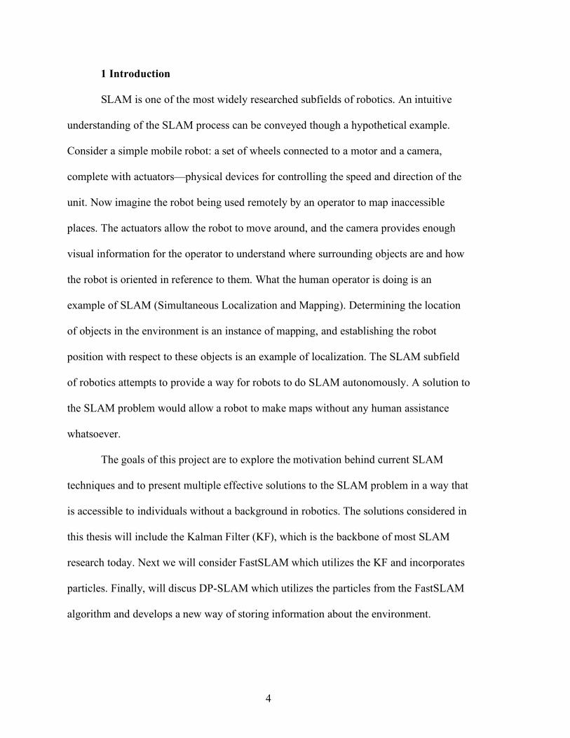
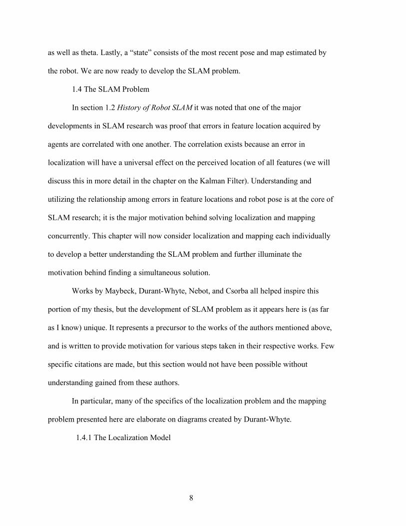
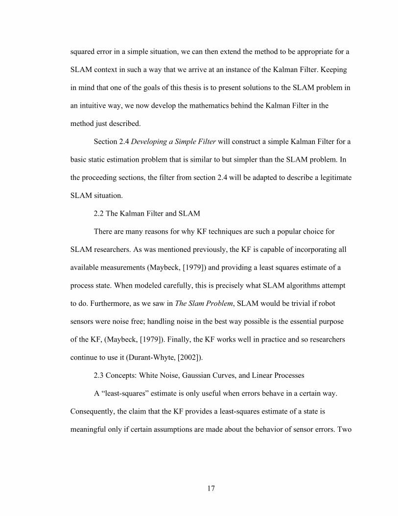
Imagine that the robot starts in some known location, x0, and has knowledge of a
set P containing several feature locations. (Notation is specified in detail in section 2.6.1
Adapted Notation for Multiple Dimensions.) The world is exactly as our robot perceives it
because the robot’s (noisy) sensors have not been needed yet. When the robot attempts to
move a given distance in a certain direction (i.e. the movement vector u1) to location x1, it
will actually move along some other vector to some location which is nearby x1. The
beacons need to be relocated to determine the new robot pose. If the actuators were
completely accurate the beacons could be reacquired by assuming they have moved
inversely to u1. Because the actuators are imprecise, however, the robot must search for
the beacons. The search is facilitated by beginning near the expected location of the
beacon and expanding outward. The following diagram presents the situation so far:
10
Notice that x1 as well as the movement vectors correspond to estimates rather than
ground truth. (This convention will be dropped briefly in section 1.4.2 The Mapping
Model but will be readopted once we begin to discus Simultaneous Localization and
Mapping; a SLAM algorithm will never have access to its actual position or movement
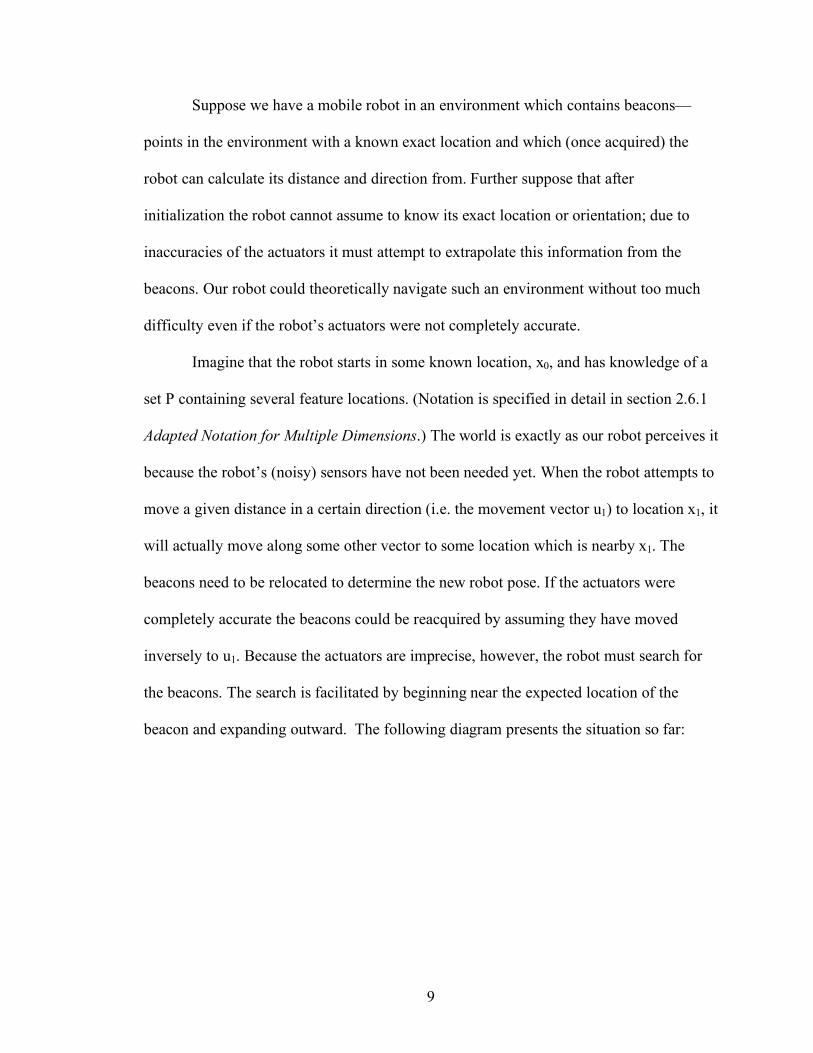
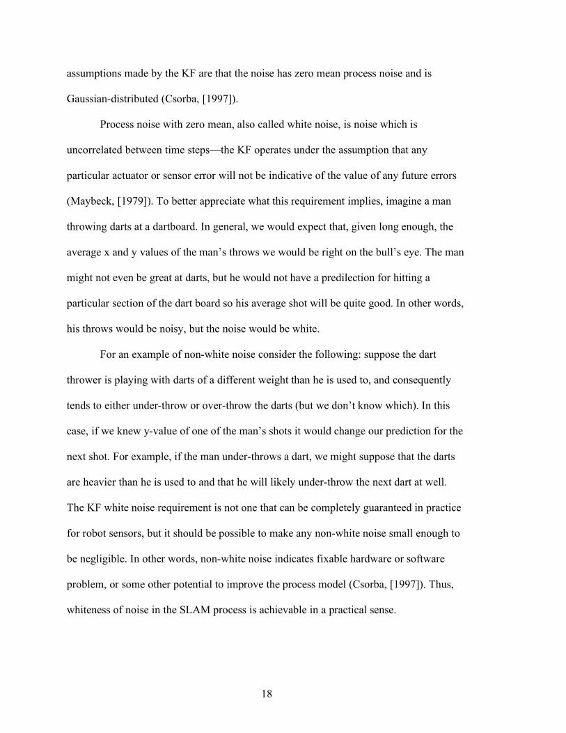
vector and will therefore have no reason to name it.) Once the beacons are reacquired, a
new robot location estimate, x2, can be made, as shown below:
Over time, the estimate of the robot pose will never diverge because the beacon
locations are fixed and known absolutely; the robot pose is always calculated from the
same correct data. We use beacons rather than features in this example simply because
Key: Position Update Vector
Observation
x0 p0
p1 x1 Feature Position:
x2
(Location estimate update based on new observations.)
Actual Movement Vector
Key:
Predicted Movement Vector
Predicted Observation
Actual Observation
x0 p0
p1
u1
x1
Actual Feature Position:
Predicted Feature Position: (Search for p1 expands outward from expected location.)
11
we would be more likely to know the absolute location of beacons than naturally-
occurring features. Note that the situation would be essentially the same if the agent
began with an accurate feature map rather than beacons. The only difference would be
that the agent would need to reacquire features from camera images rather than simply
finding beacons.
1.4.2 The Mapping Model
Mapping, in a sense, is the opposite of the situation described above. In mapping,
we assume the agent knows exactly where it is at all times—that is, we assume we either
have perfect motion sensors, or an error free GPS. What the agent lacks in the mapping
context is a way of knowing the absolute location of features. Notice that in contrast to
localization, the agent does not begin with an accurate world view; the agent can locate
features to build a map, z0 = {z00, z01 … z0n} where zij is read, “the jth feature estimate at
time step i”. Of course, z0 will only contain approximations of the actual feature
locations. When the agent moves, however, the map can generally be made more
accurate.
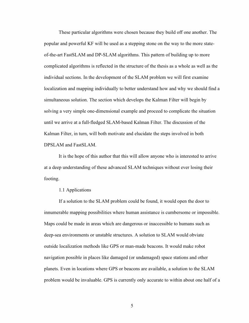
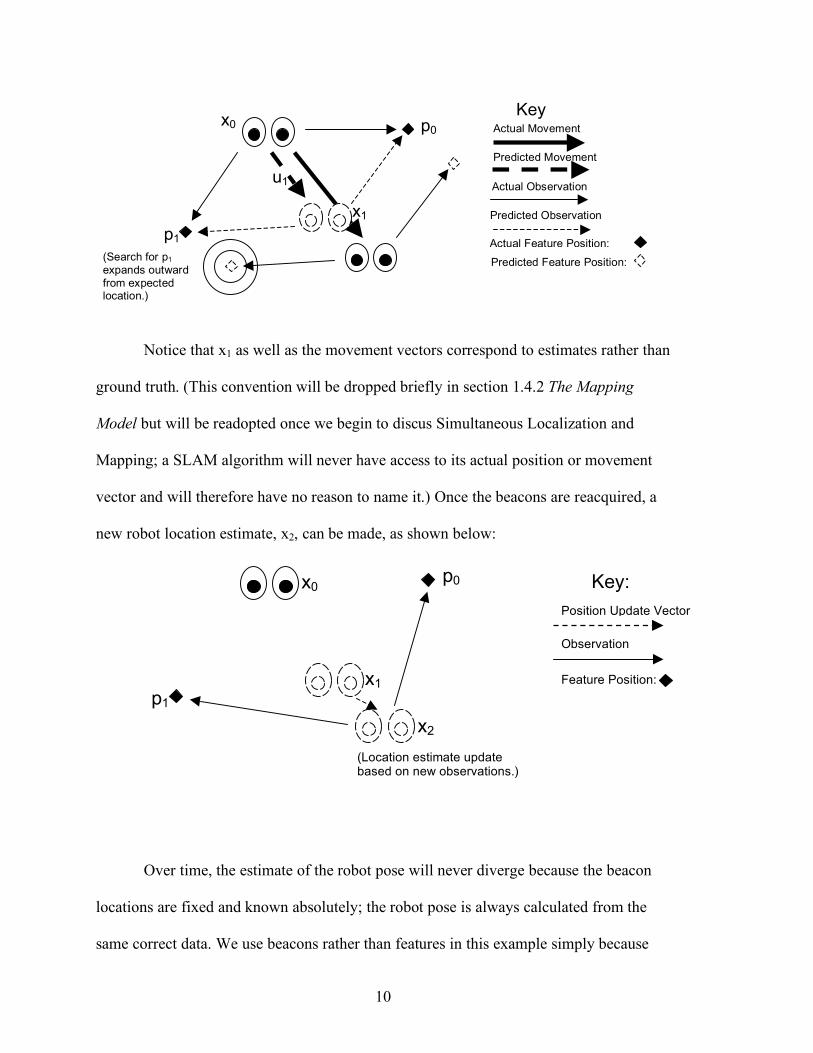
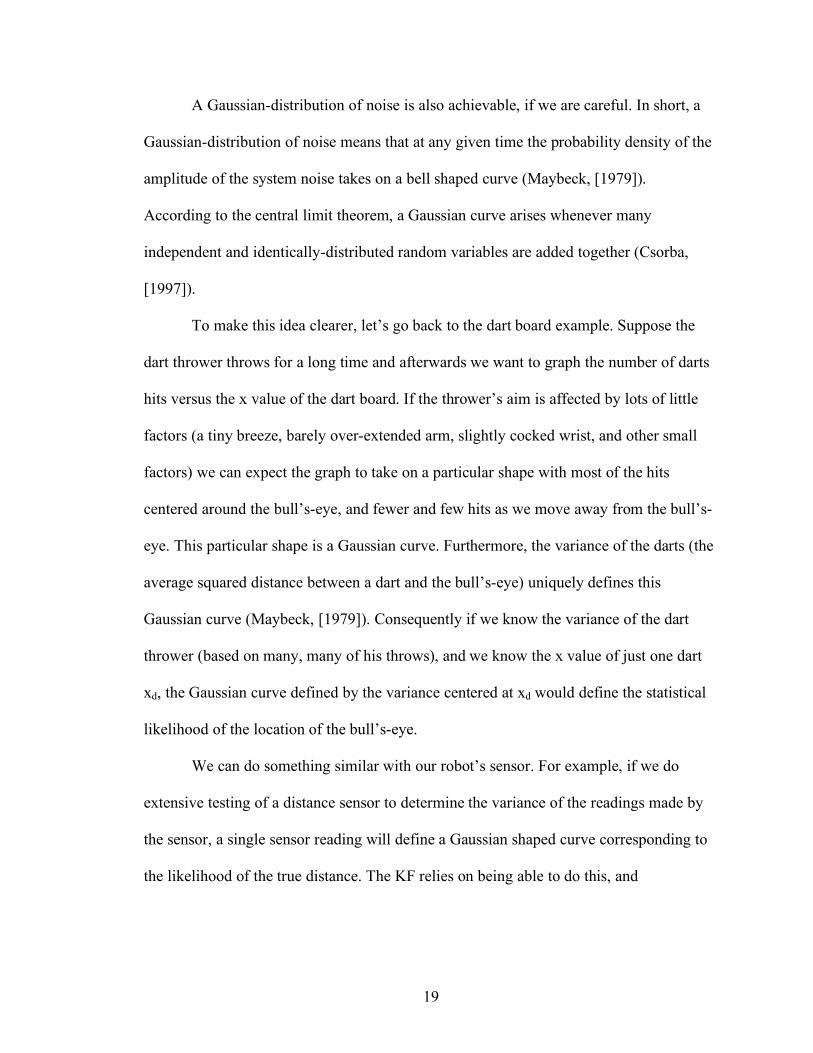
Consider the robot from the previous section beginning at x0 and moving along u1
to x1. The robot will once again need to acquire the set of features, just as it did in The
Localization Model, but this time the perceived locations of the features will have shifted
from their expected locations due to sensor inaccuracies rather than odometry
inaccuracies. The situation is the same as before, however; the features can be relocated
by searching near where the robot expects to find them. Once this is accomplished the
robot will have built a new map, z1, consisting of new locations of the features in z0.
12
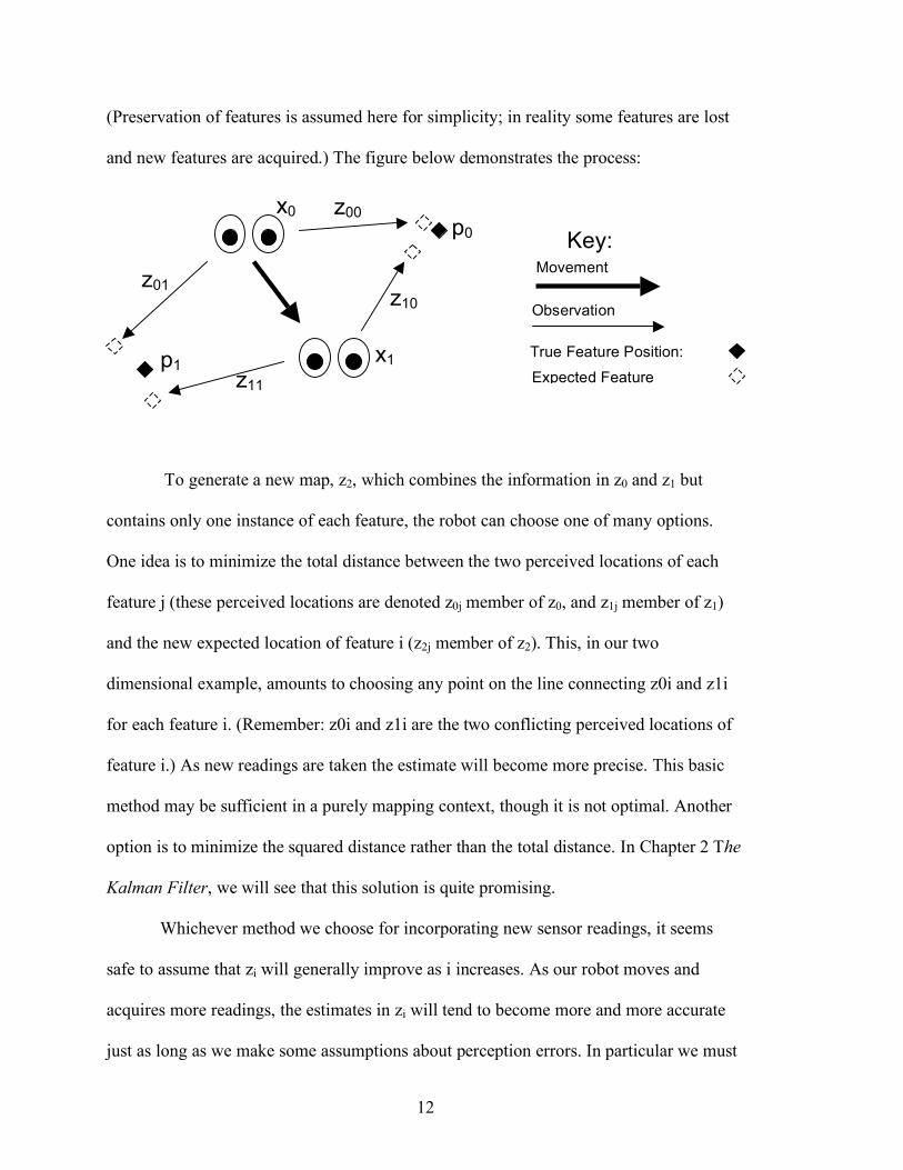
(Preservation of features is assumed here for simplicity; in reality some features are lost
and new features are acquired.) The figure below demonstrates the process:
To generate a new map, z2, which combines the information in z0 and z1 but
contains only one instance of each feature, the robot can choose one of many options.
One idea is to minimize the total distance between the two perceived locations of each
feature j (these perceived locations are denoted z0j member of z0, and z1j member of z1)
and the new expected location of feature i (z2j member of z2). This, in our two
dimensional example, amounts to choosing any point on the line connecting z0i and z1i
for each feature i. (Remember: z0i and z1i are the two conflicting perceived locations of
feature i.) As new readings are taken the estimate will become more precise. This basic
method may be sufficient in a purely mapping context, though it is not optimal. Another
option is to minimize the squared distance rather than the total distance. In Chapter 2 The
Kalman Filter, we will see that this solution is quite promising.
Whichever method we choose for incorporating new sensor readings, it seems
safe to assume that zi will generally improve as i increases. As our robot moves and
acquires more readings, the estimates in zi will tend to become more and more accurate
just as long as we make some assumptions about perception errors. In particular we must
p0
p1
x0
x1
z01
z00
z10
z11
Movement Vector
Key:
Observation
True Feature Position:
Expected Feature Position:
13
assume well calibrated sensors. If the sensor readings are routinely off to one particular
side of a feature due to poor calibration, that feature can’t be honed in on.
The assumption of proper calibration, along with other ideas from this section,
will prove invaluable throughout this project.
1.4.3 The Simultaneous Problem
Each of the algorithms described above require something as input that is
generally unavailable in practice. A localization algorithm outputs the robot pose but
requires accurate feature locations (i.e. a map) as input every time the algorithm iterates.
Conversely, a mapping algorithm generates a map but needs an undated pose as input.
The fact that the (usually unavailable) input of each process is the output of the other
suggests that the two problems are related, and could perhaps be combined into a single
solution; it seems that if both processes are utilized together there is some hope for robot
navigation without either an a-priori map or accurate GPS/odometry. One naïve solution
is considered below.
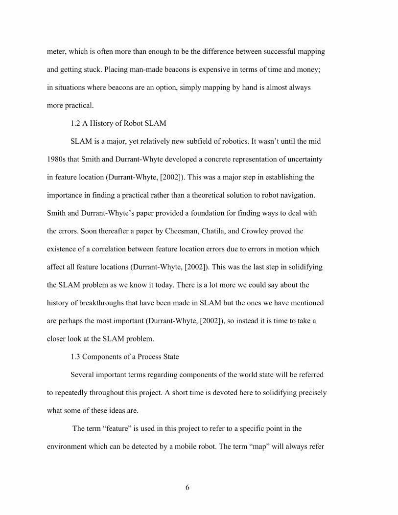
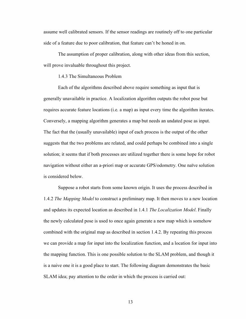
Suppose a robot starts from some known origin. It uses the process described in
1.4.2 The Mapping Model to construct a preliminary map. It then moves to a new location
and updates its expected location as described in 1.4.1 The Localization Model. Finally
the newly calculated pose is used to once again generate a new map which is somehow
combined with the original map as described in section 1.4.2. By repeating this process
we can provide a map for input into the localization function, and a location for input into
the mapping function. This is one possible solution to the SLAM problem, and though it
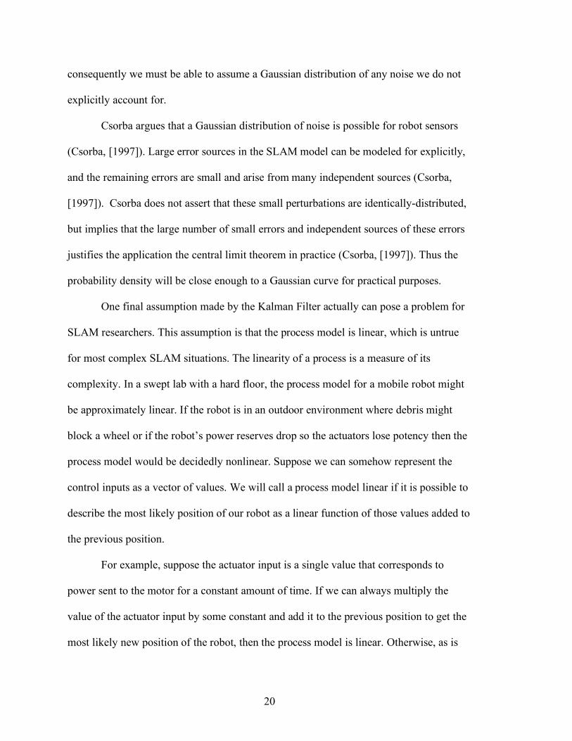
is a naive one it is a good place to start. The following diagram demonstrates the basic
SLAM idea; pay attention to the order in which the process is carried out:
14
One key thing to notice with this combined localization and mapping algorithm is
that we do not provide completely accurate input to either the mapping or the localization
components. In section 1.4.1 The Localization Model it was noted that the estimated
vehicle location would not diverge from the actual vehicle location. This was possible
because the robot pose was always estimated using accurate feature locations. Similarly,
we assumed the mapping algorithm would converge only because the robot pose is
always known exactly. Neither of these assumptions hold true in the SLAM context. Care
will be taken later to find a way to guarantee convergence of the SLAM problem in a
theoretical sense.
Another key thing to note in this preliminary solution is the significance in the
order of the two steps, localization and mapping. In the version described above, the
robot moves, updates vehicle pose, and then maps. This allows the robot to utilize the
new vehicle pose to make a better map. On the other hand, if it instead moved, mapped,
and then localized it could use the new map to make a better localization estimate. Either
way, valuable new information gets ignored in the second step. Clearly the vehicle pose
estimate and approximate map influence one another. This insight suggests a truly
1.) Make initial map z0
2.) Move, . update . location to x1
3.) Make second map, z1
4.) Update location to x using z1
5.) Update map to z using x, z0, and z1
Key: Predicted Movement Vector
Pose or feature update
Observation
True Feature Position:
Expected Feature Position:

15
simultaneous solution which takes into account the relationship between vehicle and
feature locations. This leads us to a discussion of the first rigorous mathematical solution
to the SLAM problem: the Kalman Filter.
16
2 The Kalman Filter
The Kalman Filter (or KF) was developed by R.E. Kalman, whose prominent
paper on the subject was published in 1960 (Welch and Bishop, [2006]). The KF
potential in specific localization and mapping problems was well known shortly after
Kalman published his paper in 1960. However, the KF was not generally used to
represent an entire world state (and was therefore not used as a complete solution to the
SLAM problem) until 1988 (Castellanos, Neira, Tardos, [2004]).
The Kalman Filter is an algorithm which processes data and estimates variable
values (Maybeck, [1979]). In a SLAM context, the variable values to be estimated will
consist of the robot pose, and feature locations—i.e. the world state. The data to be
processed may include vehicle location, actuator input, sensor readings, and motion
sensors of the mobile robot. In other words, the Kalman Filter can utilize all available
data to simultaneously estimate robot pose and generate a feature map. Under certain
conditions, the estimates made by the Kalman Filter are very good; in fact, they are in a
sense “optimal”. Welch and Bishop explain that the state estimates provided by the
Kalman Filter will use any available information to minimize the mean of the squared
error of the estimates with regard to the available information (Welch and Bishop,
[2006]). Another way of putting this is that the error in the state estimates made by the
Kalman Filter are minimized statistically (Maybeck, [1979]).
2.1 The “Kalman” Idea
In section 1.4.2 The Mapping Model we considered choosing expected feature
locations based on minimizing the squared error. This basic premise is the idea behind
the Kalman Filter. In fact, if we start by creating a mathematical method of minimizing
17
squared error in a simple situation, we can then extend the method to be appropriate for a
SLAM context in such a way that we arrive at an instance of the Kalman Filter. Keeping
in mind that one of the goals of this thesis is to present solutions to the SLAM problem in
an intuitive way, we now develop the mathematics behind the Kalman Filter in the
method just described.
Section 2.4 Developing a Simple Filter will construct a simple Kalman Filter for a
basic static estimation problem that is similar to but simpler than the SLAM problem. In
the proceeding sections, the filter from section 2.4 will be adapted to describe a legitimate
SLAM situation.
2.2 The Kalman Filter and SLAM
There are many reasons for why KF techniques are such a popular choice for
SLAM researchers. As was mentioned previously, the KF is capable of incorporating all
available measurements (Maybeck, [1979]) and providing a least squares estimate of a
process state. When modeled carefully, this is precisely what SLAM algorithms attempt
to do. Furthermore, as we saw in The Slam Problem, SLAM would be trivial if robot
sensors were noise free; handling noise in the best way possible is the essential purpose
of the KF, (Maybeck, [1979]). Finally, the KF works well in practice and so researchers
continue to use it (Durant-Whyte, [2002]).
2.3 Concepts: White Noise, Gaussian Curves, and Linear Processes
A “least-squares” estimate is only useful when errors behave in a certain way.
Consequently, the claim that the KF provides a least-squares estimate of a state is
meaningful only if certain assumptions are made about the behavior of sensor errors. Two
18
assumptions made by the KF are that the noise has zero mean process noise and is
Gaussian-distributed (Csorba, [1997]).
Process noise with zero mean, also called white noise, is noise which is
uncorrelated between time steps—the KF operates under the assumption that any
particular actuator or sensor error will not be indicative of the value of any future errors
(Maybeck, [1979]). To better appreciate what this requirement implies, imagine a man
throwing darts at a dartboard. In general, we would expect that, given long enough, the
average x and y values of the man’s throws we would be right on the bull’s eye. The man
might not even be great at darts, but he would not have a predilection for hitting a
particular section of the dart board so his average shot will be quite good. In other words,
his throws would be noisy, but the noise would be white.
For an example of non-white noise consider the following: suppose the dart
thrower is playing with darts of a different weight than he is used to, and consequently
tends to either under-throw or over-throw the darts (but we don’t know which). In this
case, if we knew y-value of one of the man’s shots it would change our prediction for the
next shot. For example, if the man under-throws a dart, we might suppose that the darts
are heavier than he is used to and that he will likely under-throw the next dart at well.
The KF white noise requirement is not one that can be completely guaranteed in practice
for robot sensors, but it should be possible to make any non-white noise small enough to
be negligible. In other words, non-white noise indicates fixable hardware or software
problem, or some other potential to improve the process model (Csorba, [1997]). Thus,
whiteness of noise in the SLAM process is achievable in a practical sense.
19
A Gaussian-distribution of noise is also achievable, if we are careful. In short, a
Gaussian-distribution of noise means that at any given time the probability density of the
amplitude of the system noise takes on a bell shaped curve (Maybeck, [1979]).
According to the central limit theorem, a Gaussian curve arises whenever many
independent and identically-distributed random variables are added together (Csorba,
[1997]).
To make this idea clearer, let’s go back to the dart board example. Suppose the
dart thrower throws for a long time and afterwards we want to graph the number of darts
hits versus the x value of the dart board. If the thrower’s aim is affected by lots of little
factors (a tiny breeze, barely over-extended arm, slightly cocked wrist, and other small
factors) we can expect the graph to take on a particular shape with most of the hits
centered around the bull’s-eye, and fewer and few hits as we move away from the bull’s-
eye. This particular shape is a Gaussian curve. Furthermore, the variance of the darts (the
average squared distance between a dart and the bull’s-eye) uniquely defines this
Gaussian curve (Maybeck, [1979]). Consequently if we know the variance of the dart
thrower (based on many, many of his throws), and we know the x value of just one dart
xd, the Gaussian curve defined by the variance centered at xd would define the statistical
likelihood of the location of the bull’s-eye.
We can do something similar with our robot’s sensor. For example, if we do
extensive testing of a distance sensor to determine the variance of the readings made by
the sensor, a single sensor reading will define a Gaussian shaped curve corresponding to
the likelihood of the true distance. The KF relies on being able to do this, and
20
consequently we must be able to assume a Gaussian distribution of any noise we do not
explicitly account for.
Csorba argues that a Gaussian distribution of noise is possible for robot sensors
(Csorba, [1997]). Large error sources in the SLAM model can be modeled for explicitly,
and the remaining errors are small and arise from many independent sources (Csorba,
[1997]). Csorba does not assert that these small perturbations are identically-distributed,
but implies that the large number of small errors and independent sources of these errors
justifies the application the central limit theorem in practice (Csorba, [1997]). Thus the
probability density will be close enough to a Gaussian curve for practical purposes.
One final assumption made by the Kalman Filter actually can pose a problem for
SLAM researchers. This assumption is that the process model is linear, which is untrue
for most complex SLAM situations. The linearity of a process is a measure of its
complexity. In a swept lab with a hard floor, the process model for a mobile robot might
be approximately linear. If the robot is in an outdoor environment where debris might
block a wheel or if the robot’s power reserves drop so the actuators lose potency then the
process model would be decidedly nonlinear. Suppose we can somehow represent the
control inputs as a vector of values. We will call a process model linear if it is possible to
describe the most likely position of our robot as a linear function of those values added to
the previous position.
For example, suppose the actuator input is a single value that corresponds to
power sent to the motor for a constant amount of time. If we can always multiply the
value of the actuator input by some constant and add it to the previous position to get the
most likely new position of the robot, then the process model is linear. Otherwise, as is
21
very frequently the case, the process model is nonlinear. The Kalman Filter is still useful
in many situations where the process model is nearly linear, but later we will want a KF
solution to nonlinear process models. The solution will be to develop the Extended
Kalman Filter.
The Extended Kalman Filter (EKF) is used extensively in localization and
mapping and represents the backbone of most SLAM algorithms (Durant-Whyte, [2002]).
The EKF, the primary version of the Kalman Filter used in SLAM research, is very
similar to the un-extended Kalman Filter. The claims made thus far concerning the KF
hold true for the EKF, and by the time we finish describing the KF, the extension to the
EXF will be trivial. The basic difference between the KF and the EKF is that the KF
handles only linear process models, whereas the EKF is designed to handle more
complex non-linear process models and is therefore more useful in SLAM research
(Durant-Whyte, [2002]). For now, we will be concerned with simple linear process
models and will not worry about the EKF until the end of the chapter.
2.4 Developing a Simple Filter
The following mathematical steps are based on conclusions developed in Peter S.
Maybeck’s Stochastic models, estimations, and control chapter 1. All numbered
equations originally appear in his work in some form. The circumstances described here,
however, have been changed to be more pertinent to understanding the KF from a robot
SLAM point of view. Additionally, all diagrams as well as all non-numbered steps and
derivations are original to this thesis have been incorporated to make the development of
the Kalman Filter easier to follow.
22
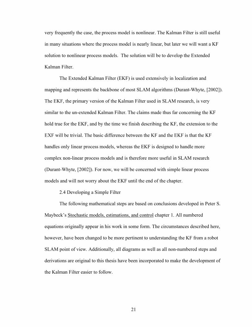
To keep things as simple as possible, let us first consider a 1-dimensional
example. Suppose a mobile robot is restricted to a line on the ground. It makes an
observation z0 and identifies a single feature p0, and uses this observation to make an
estimate of the distance between the robot and the feature x0. (Notice how these
definitions have changed subtly from Chapter 1 Introduction; these new definitions
properly reflect the simplified situation.)
Notice that the image of the robot in this diagram has changed from previous
sections. This is to convey visually that we are looking at the robot from a side view and
to remind the reader that we are now dealing with a 1-dimensional problem. This will be
a useful way to distinguish multidimensional diagrams from 1-dimensional ones.
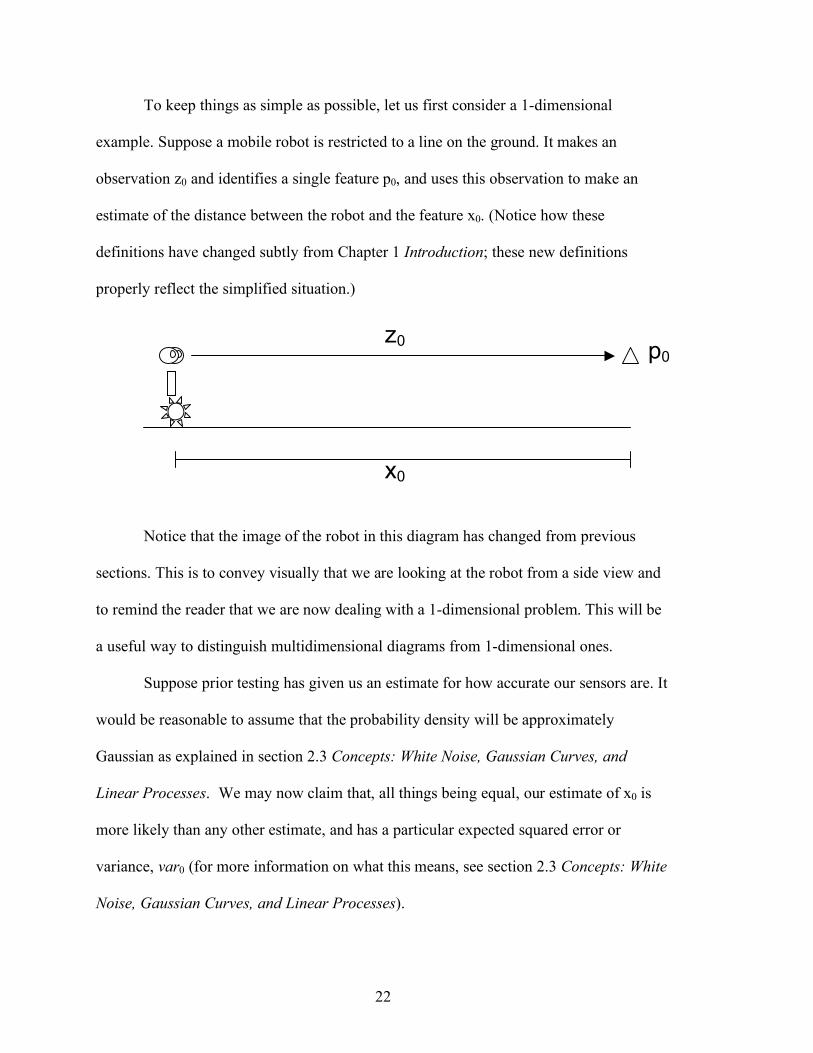
Suppose prior testing has given us an estimate for how accurate our sensors are. It
would be reasonable to assume that the probability density will be approximately
Gaussian as explained in section 2.3 Concepts: White Noise, Gaussian Curves, and
Linear Processes. We may now claim that, all things being equal, our estimate of x0 is
more likely than any other estimate, and has a particular expected squared error or
variance, var0 (for more information on what this means, see section 2.3 Concepts: White
Noise, Gaussian Curves, and Linear Processes).
z0
x0
p0
23
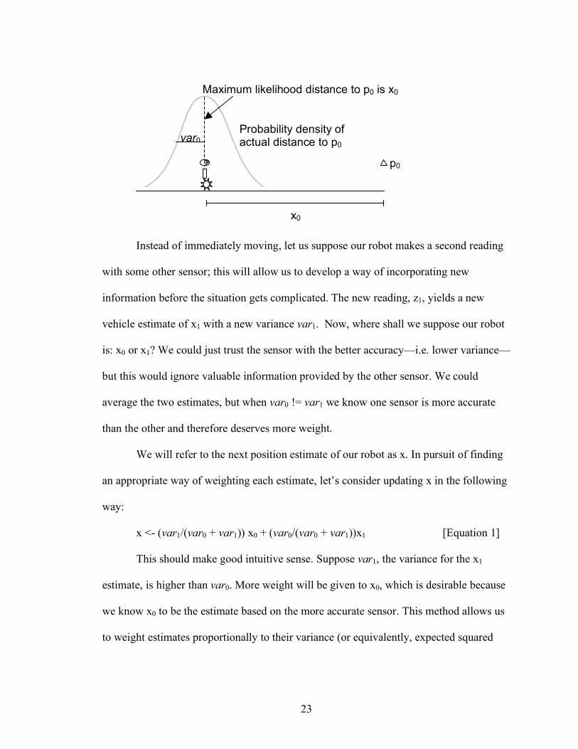
Instead of immediately moving, let us suppose our robot makes a second reading
with some other sensor; this will allow us to develop a way of incorporating new
information before the situation gets complicated. The new reading, z1, yields a new
vehicle estimate of x1 with a new variance var1. Now, where shall we suppose our robot
is: x0 or x1? We could just trust the sensor with the better accuracy—i.e. lower variance—
but this would ignore valuable information provided by the other sensor. We could
average the two estimates, but when var0 != var1 we know one sensor is more accurate
than the other and therefore deserves more weight.
We will refer to the next position estimate of our robot as x. In pursuit of finding
an appropriate way of weighting each estimate, let’s consider updating x in the following
way:
x <- (var1/(var0 + var1)) x0 + (var0/(var0 + var1))x1 [Equation 1]
This should make good intuitive sense. Suppose var1, the variance for the x1
estimate, is higher than var0. More weight will be given to x0, which is desirable because
we know x0 to be the estimate based on the more accurate sensor. This method allows us
to weight estimates proportionally to their variance (or equivalently, expected squared
x0
p0
Probability density of actual distance to p0
Maximum likelihood distance to p0 is x0
var0
24
error). It should therefore come as no surprise that the resulting value is the minimization
of the squared error with regard to the previous estimates.
Now that we have a new estimate, x, let’s consider the variance, var, of x. We
should expect that var will depend on the previous two variances, but it should be less
than either of them, i.e. var < min(var0,var1). If this is not the case, if var > var0 for
example, then by incorporating information from the second sensor we would have
actually lost information. As long as the sensors are properly calibrated this should not
happen. Fortunately, as will be explained in 2.3 Concepts: White Noise, Gaussian
Curves, and Linear Processes, proper calibration of sensors is reasonable to presume.
One would also expect var to experience the quickest (proportional) improvement
over the previous variance if the two robot sensors are equally accurate. That is,
(min(var1,var0) – var) / (var1 + var0) is maximized when var1 = var0. To see this, imagine
two independent sensors measuring the same distance. If the two sensors are equally
accurate we should be able to get a significantly better estimate (on average) by
combining the readings then by picking one in particular. If one sensor is much more
accurate than the other, on the other hand, not much information is likely to be gained by
incorporating the inaccurate sensor (although there should be some small information
gain if the readings are weighted appropriately).
The new variance can be statistically determined as follows:
1/var <- 1/var1 + 1/var0 [Equation 2]
Simple examination shows that this update equation exactly models the way we
expected the variance to behave: var < min(var1,var0) for any variances var1 and var0,
and (min(var1,var0) – var) / (var1 + var0) is maximized whenever var1 = var0.
25
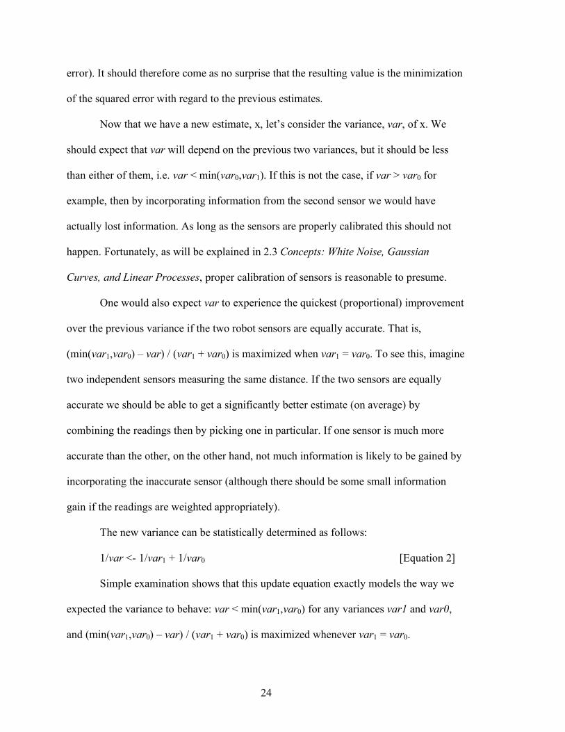
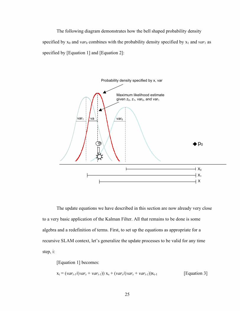
The following diagram demonstrates how the bell shaped probability density
specified by x0 and var0 combines with the probability density specified by x1 and var1 as
specified by [Equation 1] and [Equation 2]:
The update equations we have described in this section are now already very close
to a very basic application of the Kalman Filter. All that remains to be done is some
algebra and a redefinition of terms. First, to set up the equations as appropriate for a
recursive SLAM context, let’s generalize the update processes to be valid for any time
step, i:
[Equation 1] becomes:
xi = (vari-1/(vars + vari-1)) xs + (vars/(vars + vari-1))xi-1 [Equation 3]
X0
X1
X
var1 var
var0
Maximum likelihood estimate given z0, z1, var0, and var1
Probability density specified by x, var
p0
26
Where: xi is the updated location estimate at time i,
xs is a location estimate based on a new sensor reading, xi-1 is last location estimate (i.e. the best guess location based on the i-1 sensor
readings we have taken so far), vari-1 is the variance of xi-1
vars is the variance of xs
With the equation in this form we can see how to incorporate as many
independent sensor readings as we want as long as we can continue to update the
variance of the last estimate. (Updating variance will be addressed shortly.) Now let’s
perform some rearrangements to make our update equations reflect standard Kalman
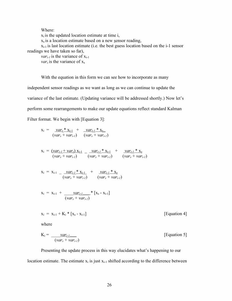
Filter format. We begin with [Equation 3]:
xi = vars * xi-1 + vari-1 * xs_ (vars + vari-1) (vars + vari-1) xi = (vari-1 + vars) xi-1 _ vari-1 * xi-1 + vari-1 * xs (vars + vari-1) (vars + vari-1) (vars + vari-1)
xi = xi-1 _ vari-1 * xi-1 + vari-1 * xs (vars + vari-1) (vars + vari-1)
xi = xi-1 + ____vari-1___ * [xs - xi-1] (vars + vari-1)
xi = xi-1 + Ki * [xs - xi-1] [Equation 4]
where Ki = ____vari-1___ [Equation 5] (vars + vari-1)
Presenting the update process in this way elucidates what’s happening to our
location estimate. The estimate xi is just xi-1 shifted according to the difference between
27
xi-1 and some new sensor derived estimate xs. The new estimate xs is weighted according
to Ki which relates the variance of the new estimate to the variance of the old estimate.
[Equation 4] is in proper Kalman Filter form (Maybeck, [1979]). All that remains now is
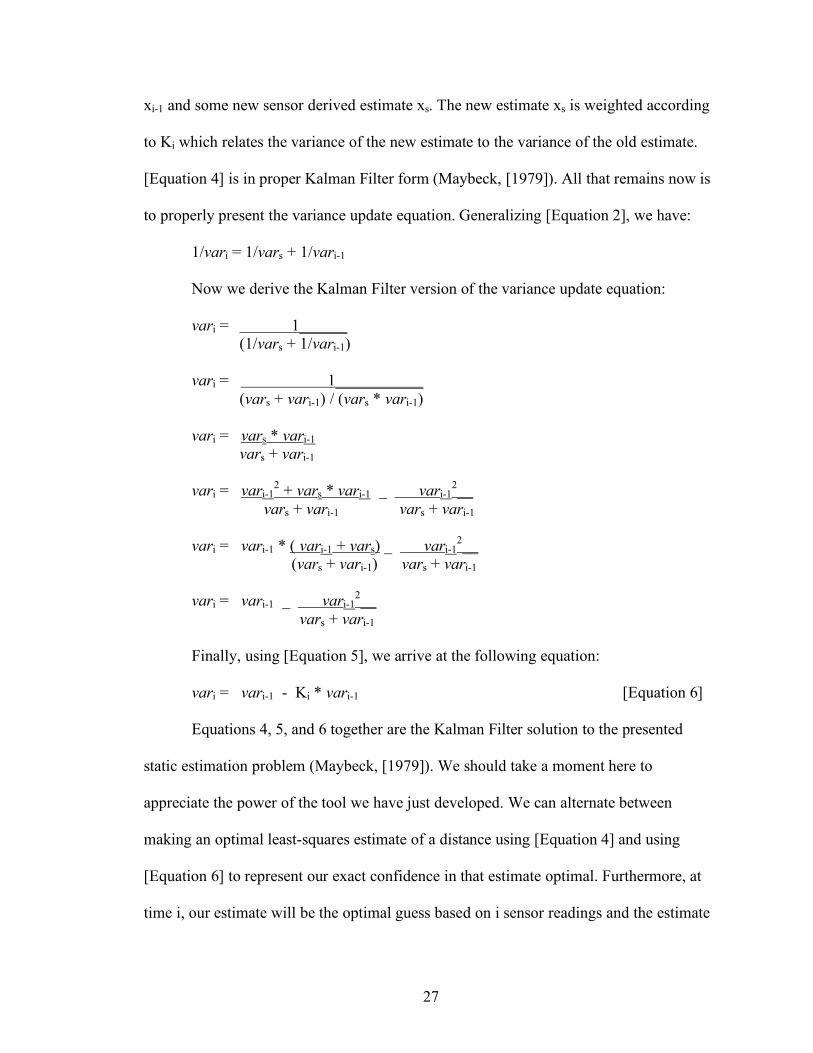
to properly present the variance update equation. Generalizing [Equation 2], we have:
1/vari = 1/vars + 1/vari-1
Now we derive the Kalman Filter version of the variance update equation:
vari = 1______ (1/vars + 1/vari-1)
vari = 1___________
(vars + vari-1) / (vars * vari-1) vari = vars * vari-1 vars + vari-1 vari = vari-1
2 + vars * vari-1 _ vari-12__
vars + vari-1 vars + vari-1 vari = vari-1 * ( vari-1 + vars) _ vari-1
2__ (vars + vari-1) vars + vari-1 vari = vari-1 _ vari-1
2__ vars + vari-1 Finally, using [Equation 5], we arrive at the following equation: vari = vari-1 - Ki * vari-1 [Equation 6]
Equations 4, 5, and 6 together are the Kalman Filter solution to the presented
static estimation problem (Maybeck, [1979]). We should take a moment here to
appreciate the power of the tool we have just developed. We can alternate between
making an optimal least-squares estimate of a distance using [Equation 4] and using
[Equation 6] to represent our exact confidence in that estimate optimal. Furthermore, at
time i, our estimate will be the optimal guess based on i sensor readings and the estimate
28
can be determined in constant time (in this static estimation problem). The fact that the
complexity of the KF does not increase with the time index combined with the fact that
the estimates made by the KF are optimal make the KF an extremely useful tool for
SLAM researchers.
We still have a fair amount of work remaining in terms of developing a KF we
can use for SLAM as we have defined. The static estimation problem above is simpler
than SLAM situations in three significant respects:
* First, the robot in the above example never actually moves. We will need to
account for vehicle translation and error in translation. (This will be relatively simple and
is handled in the next section.)
* Second, the Kalman Filter we have developed so far only considers vehicle
location with respect to a single feature. With multiple features we need to update
multiple values after every reading instead of just one.
* Third, the environment in the above example is one-dimensional. Any practical
SLAM environment will have at least two dimensions which need to be accounted for.
The solution we have developed is a good first start, however. We worked our
way up to a legitimate instance of a Kalman Filter without making any unintuitive steps.
Vectors and matrices will be needed to properly account for the last two considerations,
but the basic operations and steps will be essentially the same as those in the Kalman
Filter we developed in this section.
2.5 Developing a Kalman Filter for a Moving Robot
We ended the previous section by noticing three concerns, one of which is that we
need account for robot motion. We will now adapt our Kalman Filter to handle motion.
29
In section 2.4 Developing a Simple Filter, we were able to make progressively
better least-squares estimations by keeping track of and updating just two values: a
location estimate xi and our confidence in that estimate vari. This remains true here; to
account for control inputs made by the robot, all we need to do is figure out how control
inputs affect these two values.
Durant-Whyte suggests considering vehicle control input in a two dimensional
environment to be a vector of two values: a velocity and a heading (Durant-Whyte,
[2002]). Strictly speaking, this is already a simplification because a mobile robot will
have direct control over acceleration, not velocity. The same simplification will be made
here as modeling the physics behind robot SLAM is not a goal of this thesis. To simplify
the situation further, let’s suppose a control input simply consists of a particular velocity,
ui. (It would be redundant to specify a direction in a one-dimensional environment.) In
particular, ui refers to the control input which brought the robot from the last expected
location xi-1 to its current expected location xi for any given time step i.
Notice that if our best location estimate is xi-1 and we move at an expected
velocity ui for a length of time T, our “best guess” or expectation of the new location
estimate will just be xi-1 plus our expected movement vector. Our motion model, an
adaptation of motion models from Durant-Whyte, Maybeck, and Csorba, is therefore:
xi = xi-1 + ui * T [Equation 7]
Where T = TimeValue(i) - TimeValue(i - 1), or in other words, T is equal to the
time that has passed since the robot began moving from location xi-1.
This is all we need to do to update the location estimate xi; all that remains is to
determine how moving ought to change the confidence we have in our estimate, vari.
30
Notice that vari should depend on vari-1 (the confidence we enjoyed before control input
ui) as well as varu (the variance in the error of our actuators) weighted proportionally to
T. Also notice that vari should be greater than either vari-1 or varu as moving decreases
our expected accuracy. These two pieces of information nearly specify the update
equation. Statistics tells us that the true variance update equation is:
vari = vari-1 + varu * T [Equation 8]
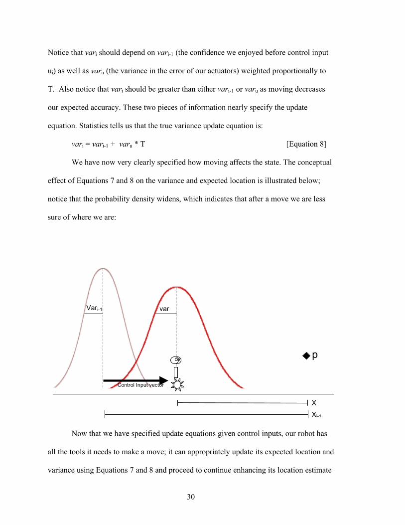
We have now very clearly specified how moving affects the state. The conceptual
effect of Equations 7 and 8 on the variance and expected location is illustrated below;
notice that the probability density widens, which indicates that after a move we are less
sure of where we are:
Now that we have specified update equations given control inputs, our robot has
all the tools it needs to make a move; it can appropriately update its expected location and
variance using Equations 7 and 8 and proceed to continue enhancing its location estimate
Xi Xi-1
Vari-1 vari
p0
Control Input vector
31
as normal by taking new feature readings. [Equation 8] was the last step in implementing
a Kalman Filter for our 1-dimensional environment. It should now be clear that non-
divergence of the SLAM problem is possible. In this particular 1-dimensional
environment, assuming we take a sensor reading after every move, we can see that as
long as Ki * vari-1 is on average greater than or equal to varu * T, over time our estimate
will always get better or stay the same.
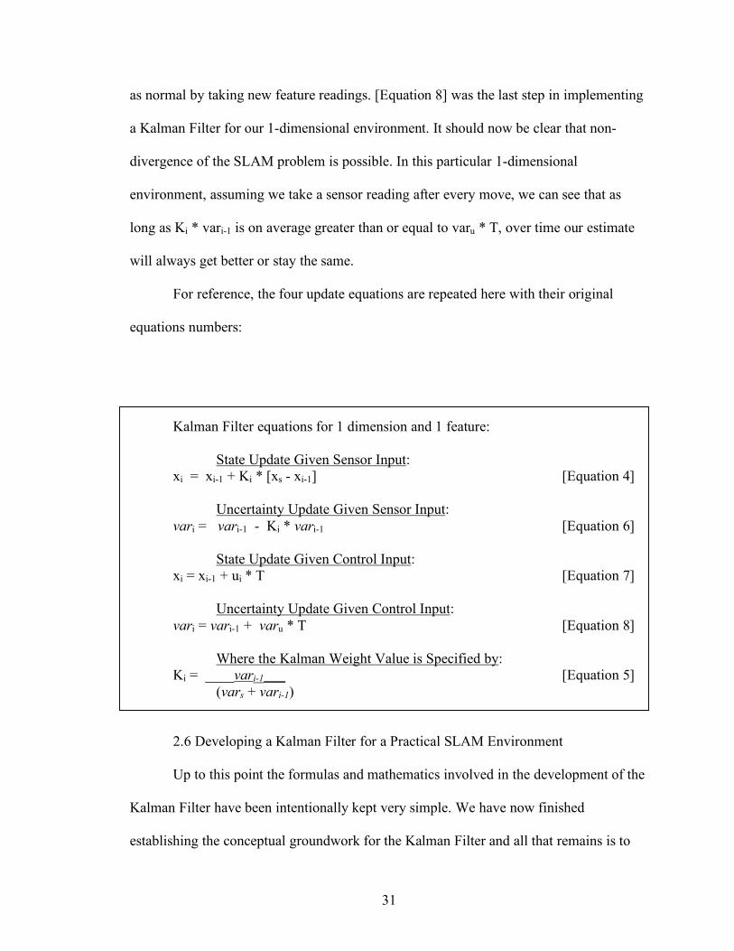
For reference, the four update equations are repeated here with their original
equations numbers:
Kalman Filter equations for 1 dimension and 1 feature:
State Update Given Sensor Input: xi = xi-1 + Ki * [xs - xi-1] [Equation 4]
Uncertainty Update Given Sensor Input: vari = vari-1 - Ki * vari-1 [Equation 6] State Update Given Control Input: xi = xi-1 + ui * T [Equation 7] Uncertainty Update Given Control Input: vari = vari-1 + varu * T [Equation 8]
Where the Kalman Weight Value is Specified by: Ki = ____vari-1___ [Equation 5] (vars + vari-1)
2.6 Developing a Kalman Filter for a Practical SLAM Environment
Up to this point the formulas and mathematics involved in the development of the
Kalman Filter have been intentionally kept very simple. We have now finished
establishing the conceptual groundwork for the Kalman Filter and all that remains is to

32
incorporate the final two considerations examined at the end of the section 2.4
Developing a Simple Filter; we will now adapt the Kalman Filter for a multi-dimensional
environment with multiple features. This will involve considerably more complex
mathematics than we have seen so far, but the basic Kalman Filter steps will be exactly
the same. We will continue to alternate between observing and moving. As before,
observing will involve estimating feature locations which we will utilize to update and
increase our confidence in the world state, and moving will provide new vantage points
for the robot while decreasing confidence in the world state.
2.6.1 Adapted Notation for Multiple Dimensions
We will need to clarify how the meaning of certain notation has changed with our
new more complicated environment. One very handy tip to keep in mind is that all
uppercase notation refers to matrices, and all lowercase notation refers to vectors. No
single valued variables will be considered (with the exception of i which will still refer to
a time step).
Perhaps the most important thing to realize is that there must now be a distinction
between feature locations and robot pose. In the previous 1-dimensional example there
was only a single measured distance. Clearly, this is no longer the case. To properly
update the state in a multidimensional environment we will need to keep track of all the
feature locations. xi will therefore refer to a vector containing both the robot pose and
updated location estimates for the features. The first element of xi, denoted xvi, will
correspond to the robot pose at time step i and the remaining elements will be feature
location estimates. Note that a vehicle pose and a feature location will need to have
33
different forms—for example, a robot pose usually needs to contain both a location and a
heading while a feature only needs a vector of coordinate values.
We need some way to refer to the feature location estimates. In our one-
dimensional example, we used the variable z to refer to observations. We can simplify
things for ourselves by modifying the meaning of z slightly to refer to actual estimates of
feature locations and just forgo notation for observations. (Naming observations was
useful to clarify the KF process, but is no longer necessary.) Additionally, we need to
adapt the notation to distinguish between multiple features at a particular time step, i. To
accommodate this, zij will refer to the jth feature location estimate at time step i, and zi
will be the vector of all observations at time step i: zi = [zi0, zi1 … zin]. Note that zi0 is a
vector specifying a physical location for feature 0.
Another very important change has to do with uncertainty. Previously we only
needed to maintain a single variance variable var, but clearly this is no longer sufficient
to model the uncertainty in the system. The uncertainty will now be contained in a
covariance matrix P which we will need to continually update.
The movement vector ui will retain its meaning as the predicted movement vector
given control input at time step i, but this must now consist of both a velocity and a
multidimensional orientation.
In the one dimensional example, Ki was a weight based on variances. Its function
will be preserved but will now correspond to a matrix of values. Similarly, a single value
to represent the uncertainty vari will no longer be adequate; we will need an entire matrix
Pi to represent uncertainty. Ki and Pi will be given more consideration shortly.
2.6.2 Adapted Movement Equations
34
The four KF update equations in this and the following section appear originally
in the PhD thesis of Michael Csorba, with only the notation changed to be appropriate to
this thesis.
In section 2.4 Developing a Simple Filter we began with simple formulas and
derived a basic version of the Kalman Filter. To do so again here for a more complicated
filter would be redundant because the same mathematical ideas are at play. The strategy
we will employ in the current and the following section will be to present the appropriate
Kalman Filter update equations at the outset and utilize the work we did in section 2.4
Developing a Simple Filter to understand each component of each equation in turn. Our
work in Developing a Simple Filter will allow us to achieve a strong understanding of the
KF as it applies to complex SLAM situations without delving too deeply into the
mathematical nuances.
In the general form of the Kalman Filter used in practical SLAM environments,
the updates necessitated by control input are handled by what are conventionally called
“prediction equations” (Csorba, [1997]). (The idea is that when we move we need to
“predict” how the state will change.) The sensor data is handled by “update equations”,
which update our state vector and uncertainty based on the data. This section will focus
on the prediction equations.
The state prediction equation given actuator input is as follows:
xi = Fi * xi-1 + Gi * ui [Equation 9]
where Fi is called the state transition matrix and Gi is a matrix which translates
control input into a predicted change in state (Csorba, [1997]). ([Equation 9] is the more
complicated version of [Equation 7].) The role of Fi is to describe how we think the state
35
will change due to factors not associated with control input. One very nice convention in
SLAM is that we get to assume that features will remain stationary. Except for the first
row which correspond to changes in vehicle pose, Fi will therefore appear as a diagonal
matrix with each diagonal entry containing identity matrices (otherwise Fi would change
location of features which we know to be stationary). If our robot can have a nonzero
velocity at time step i, then the state may change even with no actuator input, and the first
column of Fi can account for this. To simplify things a little more, however, let’s assume
that the robot comes to a halt after each time step. In this case, the actuator input fully
specifies the most likely new location of the robot. This means, Fi is just the identity
matrix (or more accurately, a diagonal matrix whose diagonal entries are identity
matrices) and can be completely disregarded. Thus, for our purposes, [Equation 9]
simplifies to:
xi = xi-1 + Gi * ui [Equation 10]
The values in Gi will depend on the representation of the control input and will
vary depending on the physical construction of the robot. Note that in [Equation 7], the
time variable T was all that was needed to perform the task which Gi must do: translate
control input to changes in state. Of course, with more control data, the translation
process is more complex and an entire matrix (i.e. Gi) is needed. As just discussed, we
will assume stationary features and therefore the only interesting entries of Gi will be in
the first row. We will not concern ourselves further with the particulars of the entries in
Gi as this is a housekeeping issue outside the scope of this essay. We can see that the only
conceptual difference between [Equation 7] and [Equation 10] is that in [Equation 10]
control input doesn’t correspond directly with a change in state, so we need matrix Gi to
36
map control into a change of state. The premise of the two equations is the same; the best
guess for our new state will be described exactly by our old pose and how we believe the
actuators will change our pose.
Now let’s take a look at the uncertainty prediction equation which is quite similar
to [Equation 8]:
Pi = Fi * Pi-1 * FiT + Qi [Equation 11]
where Qi is the covariance of the process noise (Csorba, [1997]), which will be
elaborated upon shortly. As previously discussed, we may disregard Fi which will give
the following equation:
Pi = Pi-1 + Qi [Equation 12]
To understand this equation better, let’s consider why the terms in this equation
are matrices and not vectors. The matrix Pi is now taking the role of vari. vari was our
way of measuring the uncertainty in our state prediction. There is now a unique
uncertainty value associated with each of the features as well as the robot pose. It makes
sense that we would need to keep track of multiple uncertainty values, but the reason why
we need to keep track of a matrix of values rather than a vector might be less clear. (In
particular, why don’t we use a vector of n+1 uncertainty values, where n is the number of
features?) The answer lies in what is meant by a “least squares” estimate. Before, we
were concerned our confidence in a single relationship: relative position of the robot and
the feature. Now the environment contains many more binary relationships and our
confidence feature/robot and feature/feature pair applicable. In other words, we want to
reduce the squared error in all relationships, and consequently we need to keep track of
our confidence in all relationships.
37
Let’s take a moment to consider this a bit further. Suppose that according to the
robot’s most recent state prediction, the robot’s orientation is off slightly. (In this case
suppose this simply amounts to the predicted 360-degrees bearing of the robot.) All the
feature estimates will be off as a result of this, but notice the feature estimates will all be
off in a certain manner; in addition to sensor errors, the perceived locations of the
features will all be rotated a particular angle with respect to the robot. Thus the error of
any feature in the environment is related to the error of every other feature in the
environment (Csorba, [1997]). To properly account for this fact and utilize all available
information we must keep track of our confidence in how each feature plus the robot pose
relates to every other feature and the robot pose. This is exactly the matrix, Pi.
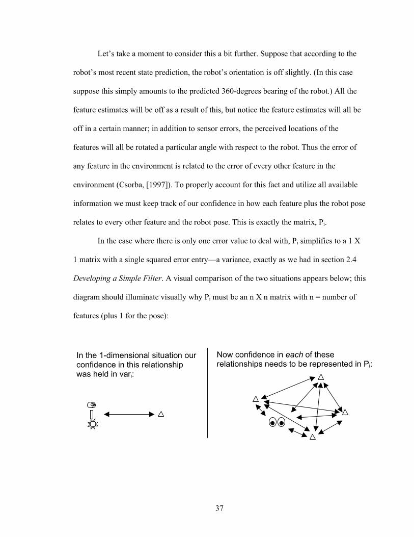
In the case where there is only one error value to deal with, Pi simplifies to a 1 X
1 matrix with a single squared error entry—a variance, exactly as we had in section 2.4
Developing a Simple Filter. A visual comparison of the two situations appears below; this
diagram should illuminate visually why Pi must be an n X n matrix with n = number of
features (plus 1 for the pose):
In the 1-dimensional situation our confidence in this relationship was held in vari:
Now confidence in each of these relationships needs to be represented in Pi:
38
Qi must account for how moving will change our confidence each individual pair
of features as well as feature-robot pairs. The entries of Qi will depend on the distance
features are away from the robot and other known particularities of the environment
and/or state. As was the case with Pi, when there is only a single confidence value to keep
track of Qi will resolve to a single variance value. With these points in mind we can see
that [Equation 8] is just a special case of [Equation 12] where there is only one
uncertainty value. We have now described mathematically what happens to our state
estimation and our confidence given actuator input according to the KF in our new
complex environment.
Before we move on, we should notice that we are well on the way to achieving an
important goal: simultaneity of mapping and localization. Notice that the matrix Pi allows
us to update our confidence in the robot pose and feature locations simultaneously.
Updating Pi amounts to updating confidence in the entire world state including both robot
pose and feature locations. Similarly (as we will see very shortly), every value in Pi can
be utilized to update the entire state given even a single sensor input. In other words, truly
simultaneous localization and mapping can be performed every time new information
becomes available. We should now understand how the Kalman Filter is a simultaneous
solution to the SLAM problem.
2.6.3 Adapted Sensor Equations
The specification of the “prediction” equations in the previous subsection leaves
only the sensor, or “update”, equations, which are used to incorporate feature estimates
based on sensor readings. These equations will be similar to Equations 4 and 6 in form,
but it will be worthwhile to examine each in turn to understand exactly how the situation
39
has changed from the 1-dimensional example. As usual we will need to update the
predicted state and our confidence in the current state using the new data. We begin with
the state update equation:
xi = xi-1 + Ki * vs [Equation 13]
where vs (also called the innovation) is an adjustment vector suggested by new
sensor readings (Csorba). Let’s look at vs and Ki more closely. vs is defined as follows:
vs = xs – Hi * xi – 1 [Equation 14]
The purpose of Hi is to transform our previous state estimate into a representation
used by the sensors. In other words, if the sensors had perceived the world state exactly
as predicted by xi-1, they would have returned this information in the form Hi * xi – 1.
(Notice that the purpose of Hi is very similar to that of Gi. Once again we need not go
into details of the matrix entries.) vs, then, is essentially just the difference between the
sensor estimate of the state, and the last cumulative estimate of the state. Substituting
using [Equation 14] we have:
xi = xi-1 + Ki * [xs – Hi * xi – 1] [Equation 15]
This equation is so similar to the one-dimensional example that the equation as a
whole can be understood conceptually from work we did to derive [Equation 4].
However, it behooves us to consider how Ki is constructed when the environment is
multidimensional and contains multiple features—once we have done so, the remaining
work in this section will be trivial. Ki is still based on the relative confidence of our
sensors versus our previous estimate as it was in section 2.4 Developing a Simple Filter,
but the variable Ki now refers to a matrix and is determined as follows:
Ki = Pi-1 * HiT * Si
-1 [Equation 16]
40
We have already discussed how Pi-1 and Hi are determined. Si is the covariance of
the innovation vi and is determined as follows:
Si = Hi * Pi-1 * HiT + Rs [Equation 17]
where Rs is the covariance matrix for the sensor noise. The difference between Ri and Si
is subtle; it may be helpful to think of Ri as the tool we use to keep track of our
confidence in our sensor readings and Si as the tool we use to keep track of our
confidence in the new state suggested by the readings given the fact that our sensor
readings differ from what we would have otherwise predicted. Note that both Ri and Si
are matrices, with dimensions one plus the number of features. In section 2.4 Developing
a Simple Filter, sensor noise could be represented with just a single variable, vars. To
understand why Si and Ri are matrices, see the arguments we used when we defined Pi in
the previous section. Combining [Equation 16] and [Equation 17] we see the Kalman
matrix constructed in this manner:
Ki = Pi-1 * HiT * [Hi * Pi-1 * Hi
T + Rs]-1 [Equation 18]
Remember that Hi and HiT just do clerical work of relating sensor data to the
world state and vice versa. If we ignore Hi and HiT, we can see clearly how [Equation 18]
is analogous to a slightly rewritten version of [Equation 5]: Ki = vari-1 * [vari-1 + vars]-1.
(Remember we said that Pi-1 is analogous to vari-1 and Rs is analogous to vars.) Of course,
the symbol -1 indicates inverse rather than power in [Equation 18], but the conceptual
function of the symbol is the same: the magnitude of the values in Ki will depend on the
previous uncertainty relative to the combined values of the previous uncertainty and
sensor uncertainty.
41
The uncertainty update equation will complete our discussion of the KF update
formulas. After we have updated our state using [Equation 13] we can update Pi as
follows:
Pi = Pi-1 – Ki * Si * KiT [Equation 19]
We have already defined all the terms in this formula. Intuitively, the purpose of
this equation is the same as the purpose of [Equation 6]. We want to update our
confidence based on the combination of the previous confidence and the sensor
confidence. Just as in [Equation 6], the new confidence will always be higher (i.e. with
lower covariance entries) than previously. Also, the new confidence will proportionally
improve most when the sensor confidence is similar to the accumulated confidence.
We have now considered prediction and update equations for both state and
uncertainty, and in so doing have specified the Kalman Filter for a multidimensional
environment with multiple features. We should take a moment here to appreciate what we
have accomplished in the last two sections. We have explained mathematically how a
robot may alternatively move and map an unknown environment with unlimited features
and multiple dimensions. We have described how to use all available knowledge in a
realistic SLAM environment to maintain an accurate confidence level in each aspect of
the state, and how to use that confidence to make the best possible state estimation given
new data. Additionally, we have taken care to make each of the four Kalman equations as
analogous as possible to the equations we rigorously developed in sections 2.4
Developing a Simple Filter and 2.5 Developing A Kalman Filter For a Moving Robot.
We have also taken care to properly explain the presence of any conceptually new aspects
of the equations which we did not see in those sections. In short, we have specified the
42
steps involved in the optimal least squares SLAM solution, and further we have explained
the purpose of each of these steps and described how they work in a careful and intuitive
manner.
Of course, there is a lot more we could says about the KF, but the goal of this
thesis is not to enumerate every detail of the Kalman Filter but rather to provide an
explanation of a few SLAM techniques in a manner that does not require a strong
background in robotics to understand. While understanding the Kalman Filter was a goal
of this thesis in and of itself, the KF will also serve as a stepping stone to other, more
state-of-the-art techniques. After a brief discussion of the Extended Kalman Filter, our
discussion of the KF will draw to a close. For reference, the equations which comprise
the KF solution presented in the last two sections are repeated here, with their original
equation numbers:
Kalman Filter equations for practical SLAM environments:
State Update Given Actuator Input: xi = xi-1 + Gi * ui [Equation 10] Uncertainty Update Given Actuator Input: Pi = Pi-1 + Qi [Equation 12] State Update Given Sensor Readings:
xi = xi-1 + Ki * vs [Equation 13] Uncertainty Update Sensor Readings: Pi = Pi-1 – Ki * Si * Ki
T [Equation 19]
Where: vs = xs – Hi * xi – 1 [Equation 14] Ki = Pi-1 * Hi
T * Si-1 [Equation 16]
Si = Hi * Pi-1 * HiT + Rs [Equation 17]
43
2.7 The Extended Kalman Filter
The Extended Kalman Filter (EKF) is very similar to the Kalman Filter.
Equations 13 and 19 are utilized unchanged in the EKF, and Equations 10 and 12 need to
be modified only slightly for use in the EKF (Csorba [1997]). An in-depth discussion of
the new equations would require the description of complex mathematical concepts and
would not contribute to our understanding of SLAM a significant way. However, the
Extended Kalman Filter deserves a little consideration here as it is more commonly
employed than the basic KF in practical SLAM situations. The reason for the popularity
of the EKF is that it can handle nonlinear process models (see section 2.3 Concepts:
White Noise, Gaussian Curves, and Linear Processes), and in most real world SLAM
situations there will be some non-linear aspect we wish to account for.
The EKF assumes that a function, f, describes how the state changes from one
time step to the next time step. The EKF further assumes f can be computed to generate a
new state estimate given a state, time index, and control input. (In a SLAM context we
are only worried how the robot pose changes, not the entire state, because we are still
assuming features are stationary.) Thus we may rewrite Equation 10 as
xi = f[xi-1, ui, i-1] [Equation 10b]
(Durant Whyte [2002]). The EKF does not assume, however, that f can be described by a
discrete equation. This causes a problem when we want to update the covariance
matrix—we can’t describe how our certainty changes when we don’t expect the state to
change in a discrete way.
To solve this problem, the EKF uses the Jacobian of f (an approximation of how
the state will change) to approximate how we should expect our certainty to change. In
44
the interest of brevity and to steering our discussion toward SLAM topics as opposed to
mathematics topics, we will forgo an in-depth discussion of the Jacobian. Put intuitively,
the Jacobian of f, Jf, is a matrix which describes how the state would change after time =
i given that the state begins to change in a linear manner at exactly time = I (Csorba
[1997]). For example, suppose a robot’s speed is changing according to some complex
function f, and at time = i the robot is slowing down at a rate of 1 meter per second or
m/s. We might expect that at time = i + 1 the robot’s acceleration will be different than 1
m/s, but the EKF would assume a constant deceleration for the purposes of calculating
the covariance matrix. The EKF update equation for uncertainty is:
Pi = Jf * Pi-1* Jf T + Qi [Equation 12b]
(Durant Whyte [2002]).
Note that if we maintain our assumption that the robot stops between each set of
observations, the Extended Kalman Filter is of no use at all; the Jacobian can be
discounted at each step because all features and the robot are stationary. We have
considered the EKF only because it is the version of the KF most frequently used in
SLAM techniques and frequent references are made to the EKF in SLAM literature. It is
important to know a little about the EKF simply to improve our understanding what most
SLAM techniques to date have focused on.
2.8 Limitations of Kalman Filter Techniques
The Kalman Filter, as we have argued, is a very good SLAM tool. One might
wonder how we can improve on an optimal least-squares approach like the KF. Of
course, given a particular physical environment and a particular robot there will be
numerous heuristics which can be combined with the KF to boost performance. However,
45
it might seem from the arguments we have made so far that the KF is in general the best
starting place for any SLAM problem. If the sheer number of variations developed by
researchers is any indication of the KF’s merit, then the KF is a good place to start
indeed; the KF is, as we have said, the basis for (by far) the majority of SLAM
approaches (Durrant-Whyte, [2002]). On the other hand, many recent solutions have
come at SLAM from other directions. It is time to consider how the Kalman Filter might
not be the best solution in many situations after all.
KF approaches work extremely well for environments in which there are a
particular number of easily trackable features (M, T, K, & W, [2002]). This is a result of
the time complexity of the KF. Remember that the covariance (uncertainty) matrix
updated by the KF, Pi, is quite large because it needs to relate each feature to every other
feature. We must update each of these values for every iteration of the filter irrespective
of how many features are actually located. Therefore, the KF has a complexity of O(m2)
for each iteration, where m is the number of features. The practical result of this is that, in
order to work in real time, the number of features must be somewhere in the ballpark of a
few hundred (M, T, K, & W, [2002]). The case can be made that the KF is doing far too
much work. For example, there is no guarantee that in practice that uncertainty values
maintained by the KF will accurately reflect the actual error in the sensors or in the state
prediction (Castellanos, Neira, Tardos, [2004]). It seems that maintaining covariances is
computationally expensive and also not always as useful in practice as it is in theory. For
these reasons, some have decided that more time should be spent on other things, for
example utilizing additional features (M, T, K, & W [2002]).
46
Most real world environments have many more than a few hundred theoretically
trackable features in them. In these environments we see the flaw in the claim that the KF
utilizes all available information; the KF certainly could take every available feature into
account, but the price might be a very long wait or the need to hand over the data to faster
hardware to be processed. In many cases, the only alternative is to ignore the vast
majority of features and consequently the vast majority of available data. It practice it is
sometime better to take every feature into account, and make up the time by using an
algorithm which represents uncertainty without a single large covariance matrix for the
feature estimates.
KF approaches suffer from another draw back in the opposite situation. Many
environments have few if any trackable features. The problem of feature tracking is a
complicated one, and we can never guarantee that a robot will be able to find a feature
again after it moves. Additionally, if there are repeating patterns in the environment the
wrong feature might be relocated or one feature might be mistaken for another. Suppose
our robot is placed in such an environment equipped with a laser range finder. The claim
that the KF utilizes all available information is not quite accurate once again; using the
laser range finder alone may be more useful than attempting to follow a few poor features
around with a KF (Eliazar and Parr, [2004]).
One final limitation of the KF which is particularly applicable to this thesis
manifests itself when the robot leaves an area in the environment and returns to it again
later. Even if the old features can be relocated, the robot may have difficulty realizing it
has already seen them and count them as new features. Intuitively, it seems that returning
to a familiar environment should improve the robot’s state rather than make it worse, but
47
the KF often requires special “loop closing” heuristics to handle the situation properly
(Eliazar and Parr, [2004]). The robot’s ability to handle previous locations is known as its
loop closing capability. Loop closing is one of the most difficult problems facing SLAM
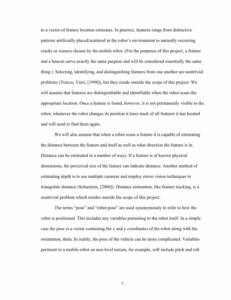
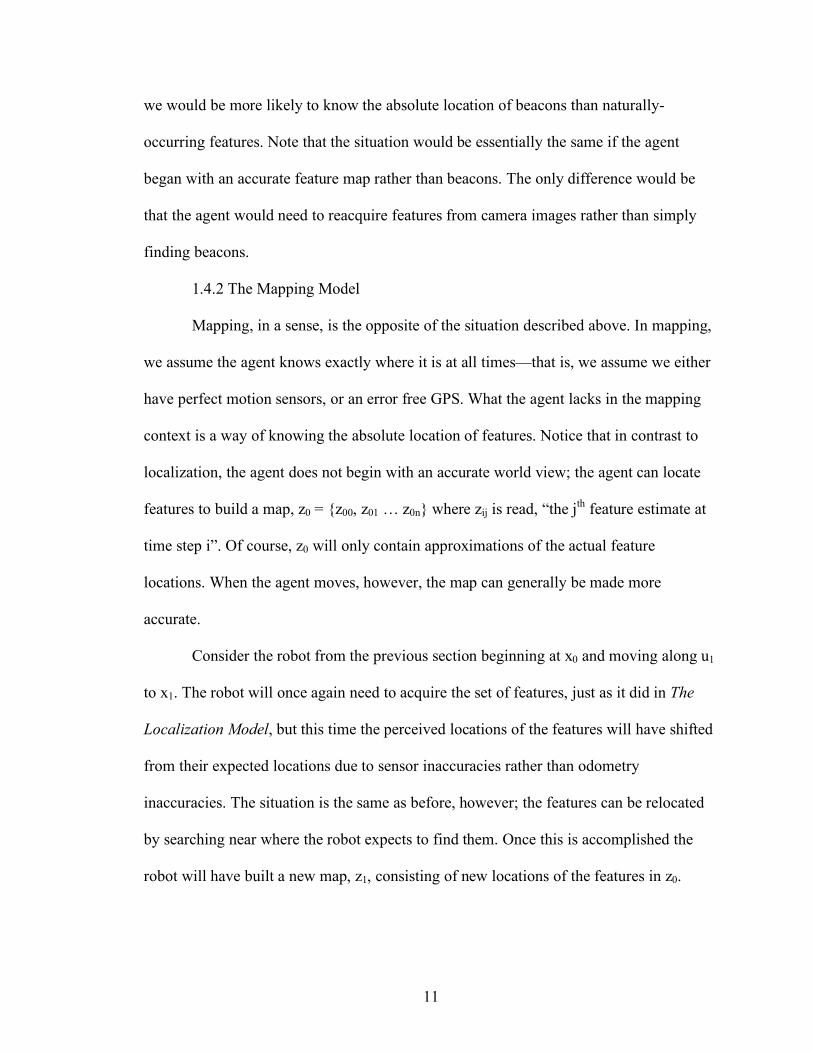
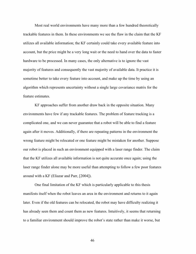
researchers today (H, B, F, & T [2003]). To see why loop closing is a problem, imagine a
robot attempting to move back to a previous position after maneuvering around some
obstacle. The accumulated errors that resulted from prolonged occlusion of familiar
features might be enough to prevent the robot from recognizing the features it previously
used. The problem of loop closing is illustrated below:
We will now take a look at two alternate SLAM methods which excel in
situations the KF is unsuited for.
x0
x5
x1
x6
Reacquiring features after many steps of occlusion can be difficult:
Accumulated location error can result in aliasing of features (i.e. poor maps)
Key
Robot location: 1st pass
Robot location: 2nd pass
Feature observation: 1st pass
Feature observation: 2nd pass
z00 != z50
Movement Vector
Observation Vector
48
3 FastSLAM
We ended our discussion of the Kalman Filter by noticing that KF based
techniques have limitations which come into play in certain situations. In particular, we
noticed that in environments where millions of features are available, relatively few can
be utilized by the KF in a reasonable amount of time. This is the particular limitation of
the KF that FastSLAM attempts to improve upon. FastSLAM was developed by
Montemerlo, Trun, Koller, and Wegbreit who published a definitive paper on the
algorithm in 2002 (M, T, K, & W, [2002]). FastSLAM breaks up the problem of
localizing and mapping into many separate problems using conditional independence
properties of the SLAM model (we will discuss exactly what is meant by this shortly). In
brief, FastSLAM is capable of taking far more raw sensor data into account by
concentrating on the most important relationships between elements in the environment.
The result is a SLAM solution that performs much better than the KF in many
environments. For example, environments with many random patterns, shapes, and
textures often work quite well for the FastSLAM algorithm.
3.1 A Bayesian Approach to SLAM
FastSLAM suggests presenting the SLAM problem from a Bayesian point of view
(M, T, K, & W, [2002]). A Bayesian model of the world is one in which there are certain
“random variables”—variables which take on different values with different probabilities
depending on the values returned by other variables. The result is a tree of random
variables which depend on one another, and specify the likelihood of different world
states. This network is called a Bayesian network. One of the main reasons for
representing processes with a Bayesian network is so that conditional independences can
49
be taken advantage of (to be explained shortly). It can be argued that to some extent we
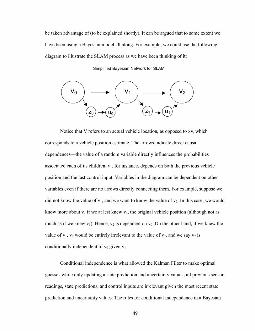
have been using a Bayesian model all along. For example, we could use the following
diagram to illustrate the SLAM process as we have been thinking of it:
Notice that V refers to an actual vehicle location, as opposed to xvi which
corresponds to a vehicle position estimate. The arrows indicate direct causal
dependences—the value of a random variable directly influences the probabilities
associated each of its children. v1, for instance, depends on both the previous vehicle
position and the last control input. Variables in the diagram can be dependent on other
variables even if there are no arrows directly connecting them. For example, suppose we
did not know the value of v1, and we want to know the value of v2. In this case, we would
know more about v2 if we at lest knew v0, the original vehicle position (although not as
much as if we knew v1). Hence, v2 is dependent on v0. On the other hand, if we knew the
value of v1, v0 would be entirely irrelevant to the value of v2, and we say v2 is
conditionally independent of v0 given v1.
Conditional independence is what allowed the Kalman Filter to make optimal
guesses while only updating a state prediction and uncertainty values; all previous sensor
readings, state predictions, and control inputs are irrelevant given the most recent state
prediction and uncertainty values. The rules for conditional independence in a Bayesian
v0 v1 v2
Simplified Bayesian Network for SLAM:
z0 u0
u1 z1
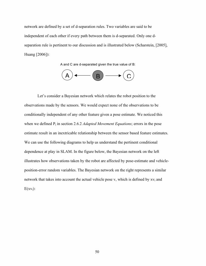
50
network are defined by a set of d-separation rules. Two variables are said to be
independent of each other if every path between them is d-separated. Only one d-
separation rule is pertinent to our discussion and is illustrated below (Scharstein, [2005],
Huang [2006]):
Let’s consider a Bayesian network which relates the robot position to the
observations made by the sensors. We would expect none of the observations to be
conditionally independent of any other feature given a pose estimate. We noticed this
when we defined Pi in section 2.6.2 Adapted Movement Equations; errors in the pose
estimate result in an inextricable relationship between the sensor based feature estimates.
We can use the following diagrams to help us understand the pertinent conditional
dependence at play in SLAM. In the figure below, the Bayesian network on the left
illustrates how observations taken by the robot are affected by pose-estimate and vehicle-
position-error random variables. The Bayesian network on the right represents a similar
network that takes into account the actual vehicle pose v, which is defined by xvi and
E(xvi):
A B C
A and C are d-separated given the true value of B:
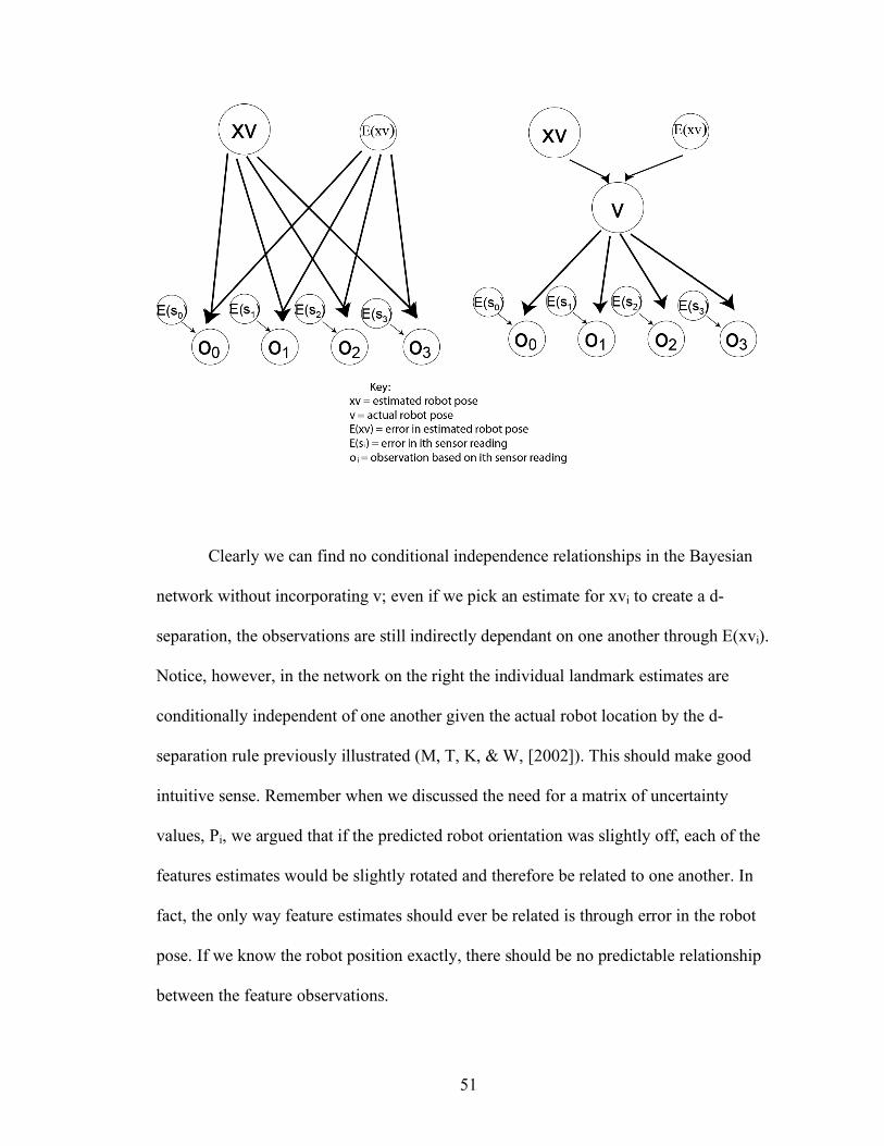
51
Clearly we can find no conditional independence relationships in the Bayesian
network without incorporating v; even if we pick an estimate for xvi to create a d-
separation, the observations are still indirectly dependant on one another through E(xvi).
Notice, however, in the network on the right the individual landmark estimates are
conditionally independent of one another given the actual robot location by the d-
separation rule previously illustrated (M, T, K, & W, [2002]). This should make good
intuitive sense. Remember when we discussed the need for a matrix of uncertainty
values, Pi, we argued that if the predicted robot orientation was slightly off, each of the
features estimates would be slightly rotated and therefore be related to one another. In
fact, the only way feature estimates should ever be related is through error in the robot
pose. If we know the robot position exactly, there should be no predictable relationship
between the feature observations.
52
Of course, a very major point in SLAM is that we do not know the exact robot
pose, but the insight of conditional independence of features given the pose is enough to
motivate FastSLAM, which handles each feature separately. The thinking is, perhaps the
relationships between features aren’t worth keeping track of if we can make a good
enough estimate (or estimates) of the random variable that, when known exactly, d-
separates all feature estimates from one another. This variable is, as just described, the
true robot pose.
3.2 The FastSLAM Algorithm
Let’s take a look at how the conditional independences described above allow us
to divide up the SLAM problem. We will need the use of a probability operator, p. Given
any input, p returns the probability of that input. For example, suppose our robot’s one-
dimensional position is specified by the variable x. Then p(x) will approximately be a
Gaussian curve, just as we saw in section 2.4 Developing a Simple Filter. If x is a
multidimensional vehicle pose and feature estimates, p(x) defines the likelihood of all
possible world states. | is the “given” operator. p(x | {u0, u1, … ui}, {z0, z1, … zi})
therefore describes likelihood of any world state given all sensor and movement data
taken by the robot at any time i, just as Pi and xi did in the more complex version of the
Kalman Filter. (For compactness, we will say Ui = {u0, u1, … ui} and Zi = {z0, z1, … zi}.)
One of the benefits of the Kalaman Filter was that no matter how large i became, Pi and xi
remained the same size as long as we kept using the same features. The unbounded nature
of p(x | Ui, Zi) as i increases is something we will need to deal with later. Notice that xi
referred to a specific world state, while x refers to all world states. x can, as would be
expected, broken down into vehicle pose, v, and feature locations p0, p1, … pm. Like x,
53
these variables represent all possible locations and poses. We can break down p(x | Ui,Zi)
as follows.
p(x | Ui,Zi) = p(v,p0,p1,…pm | Ui,Zi)
We will now use some probability arithmetic to simplify the SLAM problem.
Suppose we have two random variables which are not related, A and B. We could say,
p(A, B) = p(A) * p(B). If the value of A depended on the value of B, this identity would
not be valid. (To see why this is true, suppose A and B were either true (1) or false (0)
each with a probability of .5, that A always equaled B, and somehow we discovered that
A was 1. The left side of the expression would be 1 and the right would be .5.) If A does
depend on B, the proper factorization is p(A, B) = p(A) * p(B|A). We know our feature
predictions depend on the state prediction which means we can break
p(v,p0,p1,…pm | Ui,Zi) down as follows:
p(v,p0,p1,…pm | Ui,Zi) = p(v | Ui,Zi) * p(p0,p1,…pm | Ui,Zi,v)
We can now see how the independence relationship we discovered in section 3.1
A Bayesian Approach to SLAM might help us. Because feature observations are
conditionally independent of one another given the robot pose, and we (hopefully) have a
good approximation of the robot pose, it seems as though we might break p(p0,p1,…pm |
Ui,Zi,v) up into separate probability statements. Of course, all we can really have are
estimates for v, but if we have acurate enough estimate (or as we will discuss shortly,
enough estimates) we can make use of the following factorization:
p(v | Ui,Zi) * p(p0,p1,…pm | Ui,Zi,v)
54
= p(v | Ui,Zi) * p(p0 | Ui,Zi,v) * p(p1 | U
i,Zi,v) * … p(pm | Ui,Zi,v)
To summarize, we have:
p(x | Ui,Zi) = p(v | Ui,Zi) * ∏m p(pm | Ui,Zi,v) [Equation 20]
(M, T, K, & W, 2002).
Let’s take a moment to think about exactly what this factorization accomplishes.
We have broken the SLAM problem into m+1 separate problems, and none of the m
feature estimation problems are related to one another. It seems that this might help us
solve the cause of the polynomial complexity of the KF. (Of course, we need to develop a
way to solve each of these m+1 problems in a timely manner, but intuitively this should
seem possible.) The only price we pay for utilizing this factorization is a possible
decrease in accuracy due to ignoring correlations in feature location errors due to
inaccuracies in the predicted robot pose. An interesting result of all of this is that if we
were ever were to have 100% confidence in our robot pose, our conditional independence
assertion would be completely applicable and we could disregard correspondences
between features. In this case, solving the factorized version of the SLAM problem in
[Equation 20] would yield an optimal guess for feature locations far faster than a KF
approach.
Furthermore, if we knew the true robot pose to be one of only a finite number n, it
would still be possible to utilize the factorization in [Equation 20] as long as we knew the
likelihood of each of the n possible poses. For example, we could make a separate map
for each robot pose (each time disregarding feature error correlations) and then weight
each map accordingly. This would properly account for the correlation between
observations, and therefore generate an optimal state estimate. Additionally, this would
55
likely have a better time complexity than a KF approach, depending on the number of
features and the number of pose possibilities. In practice, there will be few if any cases
where we can narrow the possible poses to a finite number. However, if we keep track of
many possible poses and weight the likelihood of each appropriately, we might be able to
approximate the optimal least squares guess sufficiently for all practical purposes while
doing far less work than a KF. This is exactly the strategy employed by FastSLAM (M,
T, K, & W, [2002]).
3.3 FastSLAM and Particles
The FastSLAM algorithm keeps track of many possible paths simultaneously (M,
T, K, & W, [2002]). Notice that the KF does not even keep track of a single path, but
rather updates a single robot pose—the latest step in the robot path. FastSLAM records
paths so that when the algorithm terminates there will be a record of where the robot has
been and where it stopped along the way; FastSLAM does not use old poses in the paths
for any calculations, so old pose estimates are essentially forgotten during execution (M,
T, K, & W, [2002]). As the full robot paths are not utilized and therefore unimportant to
the SLAM problem as we have defined it, we will present a slightly adapted FastSLAM
algorithm which updates pose estimates rather than grows robot paths. This will simplify
notation and generally make the formulas look more familiar to ones we have seen
already in this thesis.
Maintaining multiple pose estimates at each time index necessitates a
complication of our notation for robot pose. Previously, xvi referred to the vehicle pose at
time i. Now xvi will refer to the set of robot poses we have maintained at time i. xvij will
56
refer to the jth pose estimate at time i. Therefore we have, xvi = {xi0, xi1, … xiM}, and each
estimate xij is called a particle. Now we need to specify how to update xvi.
3.4 Pose Estimation
The particles in xvi will be updated in a probabilistic way—that is to say, there
will be a certain amount of randomness involved in updating the particles. We don’t want
our particles to be homogeneous, and we also want a greater percentage of “good”
estimates to survive. This is what updating xvi probabilistically allows. FastSLAM is
only an approximation of the least squares estimate, so we will not invalidate any
optimality claims by doing this.
We will now discuss how to maintain the particle set. Suppose we have a set of
pose estimates xvi-1, and we have a control input ui. The particle set is not updated until
we make some feature location estimates from observations in our new location. Instead,
we create, xvt, a temporary set of particles based on ui and the M particles in xvi-1. Both
the number, M, of particles we maintain in the filter, and the number we generate for xvt
will depend on the situation. Testing of FastSLAM in practical situations has shown that
increasing the number of features can reduce the number of necessary particles (M, T, K,
& W, [2002]). xvt will be chosen probabilistically by sampling from xvi-1. For example,
to generate a particle for xvt we start with a particle from xvi-1, say xv(i-1),j. We then use
the probability density specified by xv(i-1),j + ui to choose temp, a new particle for xvt.
This process is illustrated below:
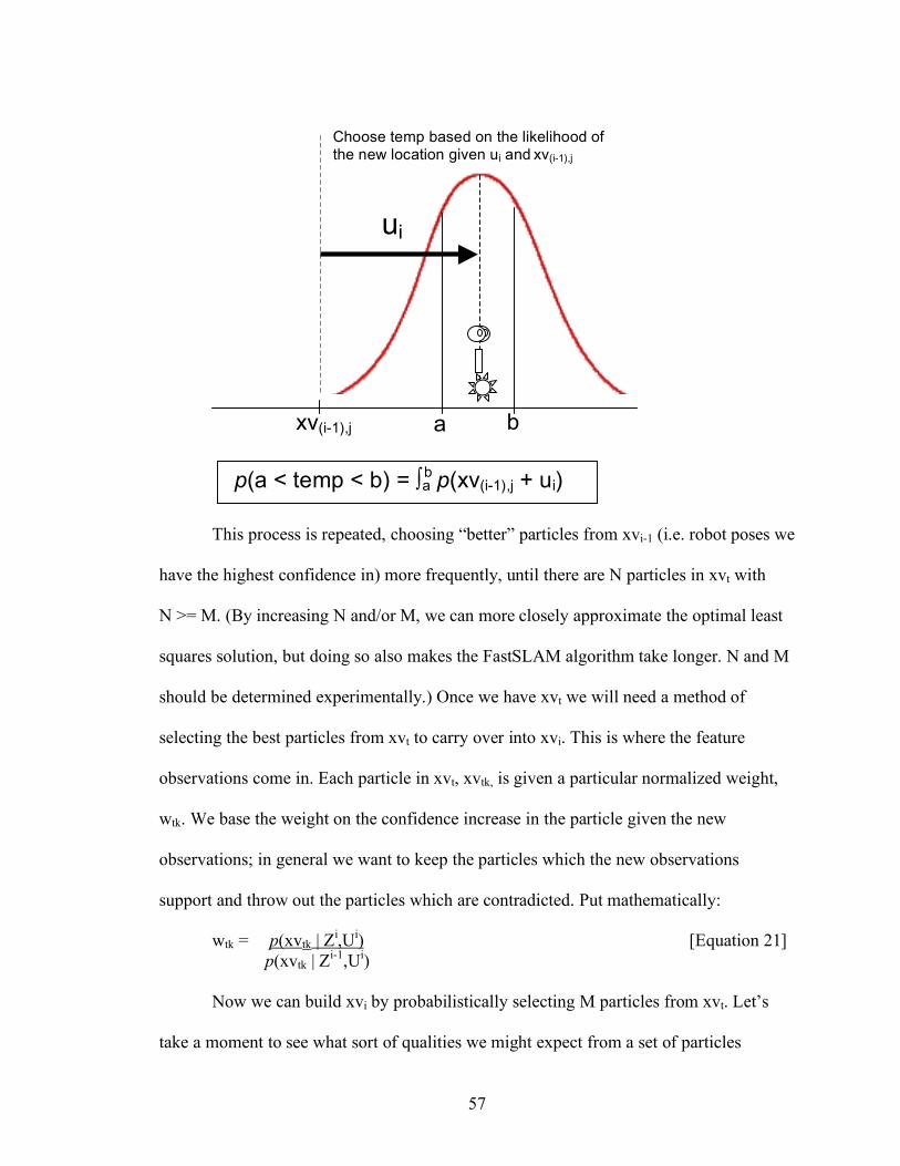
57
This process is repeated, choosing “better” particles from xvi-1 (i.e. robot poses we
have the highest confidence in) more frequently, until there are N particles in xvt with
N >= M. (By increasing N and/or M, we can more closely approximate the optimal least
squares solution, but doing so also makes the FastSLAM algorithm take longer. N and M
should be determined experimentally.) Once we have xvt we will need a method of
selecting the best particles from xvt to carry over into xvi. This is where the feature
observations come in. Each particle in xvt, xvtk, is given a particular normalized weight,
wtk. We base the weight on the confidence increase in the particle given the new
observations; in general we want to keep the particles which the new observations
support and throw out the particles which are contradicted. Put mathematically:
wtk = p(xvtk | Zi,Ui) [Equation 21]
p(xvtk | Zi-1,Ui)
Now we can build xvi by probabilistically selecting M particles from xvt. Let’s
take a moment to see what sort of qualities we might expect from a set of particles
xv(i-1),j
ui
a b
p(a < temp < b) = ∫a p(xv(i-1),j + ui) b
Choose temp based on the likelihood of the new location given ui and xv(i-1),j
58
maintained in this fashion. We choose xvt so that most of the particles/poses are close to
what we would expect them to be given our previous particles and control input. Then the
temporary particle set, xvt, is whittled down, and particles which do not reflect the new
sensor readings as well as we expected them to tend to drop away. In short, we maintain a
set of poses/particles which tend to cluster around the optimal estimate of the robot pose
given all sensor data and control input—i.e. the estimate which would be made by the
KF. In other words, xvi represents an approximation of p(v | Zi,Ui), and the error in this
approximation approaches zero as M, the number of particles approaches infinity (M, T,
K, & W).
3.5 Feature Estimation
It may be surprising to know that we are almost finished detailing the operation of
the FastSLAM algorithm. We did, after all, break the SLAM problem into m + 1 separate
problems, and we have solved only one of these. The remaining m problems, however, all
refer to feature locations estimates and can therefore be handled in the same way. All we
need is some way of estimating the now uncorrelated landmark values very quickly. We
have, quite conveniently, already developed such a method in this thesis, in section 2.4
Developing a Simple Filter. Ironically, it was the limitations of the KF which motivated
consideration of FastSLAM in this thesis, and now we will be using multiple simple
Kalman Filters in the implementation of FastSLAM.
We need not dwell on the Kalman Filter implementation in the FastSLAM
algorithm as we have already discussed Kalman Filters in detail, but some consideration
of complexity is in order. We will need to have 1 Kalman Filter per feature, per particle,
for a total of M * m filters. Each filter will be conditioned on its respective particle pose,
59
and will need to estimate one feature position. In two dimensions, we can uniquely
identify a feature location with a range and bearing—just two variables as opposed to the
m variables we had in section 2.6 Developing A Kalman Filter for a Practical SLAM
Environment. The covariance matrix for each filter, then, will be 2 X 2, and contain only
four values. (We cannot deny a correlation between error in range and error in bearing,
and consequently we will need all four values. This will take some time, but does not
change the time complexity.) This means that each filter will be only slightly more
complicated than the one we developed in 2.4 Developing a Simple Filter, and the filter
update can still iterate in constant time.
3.6 Loop Closing with FastSLAM
Loop closing, to a certain extent, is handled naturally by FastSLAM. The overall
increase in mapping accuracy made possible by utilizing this quantity of landmarks can
often prevent problems with loop closing (M, T, K, & W, [2002]). It is worth while
mentioning that FastSLAM’s system of weighted particles has inspired researchers (such
as Stachniss and Burgard) to develop active loop closing techniques. We will briefly
discuss how such techniques work.
Earlier we said that each particle in the temporary set is given a weight based on
new observations. When the robot enters a new area, the robot has no idea what the area
should look like, so the new observations are not likely to contradict any of the particles
more than others. Consequently, the weights of all the particles are likely to be similar
(Stachniss, Burgard [2004]). When the robot reenters an old area, on the other hand, one
of two things can happen. The first possibility is that some particles will make good
estimates while others won’t. In this case, the weights will be diverse and bad particles
60
are more likely to be weeded out. The other possibility is that all the particles will make
bad estimates and the loop will be closed poorly even by the best particle. This is second
possibility is more likely the case when the robot has been away for a long time.
From these arguments it seems that reentering old areas a soon as possible is
beneficial (Stachniss, Burgard [2004]). Indeed, experimental testing has confirmed this
idea. In 2004 Stachniss and Burgard attempted mapping hallways first allowing the robot
to revisit an old area half way through. They then repeated the experiments without
allowing revisitation. The maps resulting from the “revisitation” routes resulted in much
more accurate maps (Stachniss, Burgard [2004]). Stachniss and Burgard also developed
some heuristics which a robot can use to decide what area to explore next, but to go into
them here would mean staying too far from the main drive of this thesis.
3.7 FastSLAM as a Practical Real-Time Solution
The computational complexity of FastSLAM as we have described it (for a single
observation) is O(m * M), or the number of feature multiplied by the number of particles.
The O(m * M) run time is a result of copying old maps for the new set of particles. If,
instead of copying each map, we change the appropriate feature in each particle, we can
lower the complexity significantly. Sorting through the m features can be done in log(m)
time if we use a tree structure to store the maps. Storing features in this way results in a
total complexity of O(M * log(m)). This is in contrast to KF approaches which run in
O(m2) time given even a single observation.
Experimental testing has shown that in general, a few particles will suffice
irregardless of the number of features, so the complexity of FastSLAM tends to be far
better than the complexity of the KF (M, T, K, & W, [2002]). FastSLAM has been tested
61
in physical environments with as many as 50,000 landmarks, which were mapped
accurately with as few as 250 particles (M, T, K, & W, [2002]).
If we used a Kalman Filter to keep track of the same number of features, it would
need to make more than 2.5 billion covariance updates given even a single observation of
a single landmark. Clearly FastSLAM represents a vast improvement over the KF given
an environment where tens of thousands of features need to be mapped, particularly when
we consider the improved loop closing potential of FastSLAM.
To summarize, FastSLAM is based on the conditional independence of features
given an accurate robot pose. The SLAM problem can be broken into m + 1 separate
estimation problems if we can account for errors in the robot pose. We approximate the
optimal state estimate by keeping track of multiple pose estimates (i.e. particles) and
weighting the map based on each particle appropriately. The particles are maintained by
probabilistically sampling from the previous poses, and probabilistically removing poses
which do not reflect new sensor data. The result is an approximation of the optimal
mapping algorithm which executes in real time with tens of thousands of features.
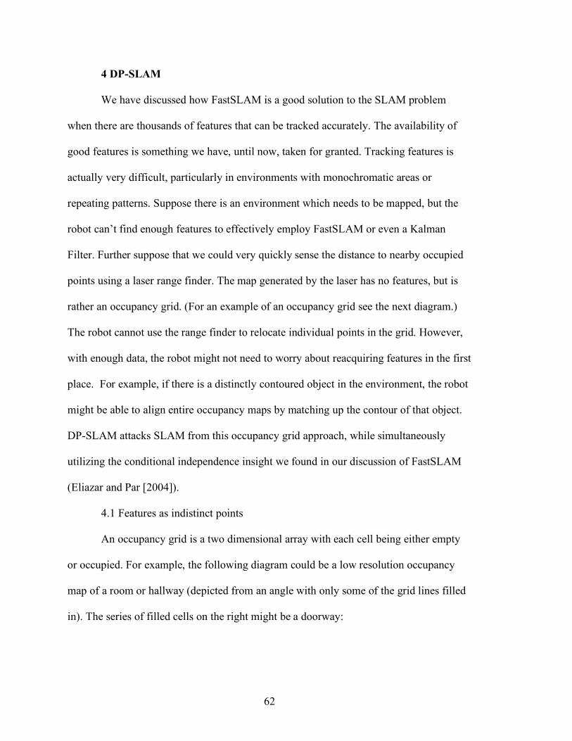
62
4 DP-SLAM
We have discussed how FastSLAM is a good solution to the SLAM problem
when there are thousands of features that can be tracked accurately. The availability of
good features is something we have, until now, taken for granted. Tracking features is
actually very difficult, particularly in environments with monochromatic areas or
repeating patterns. Suppose there is an environment which needs to be mapped, but the
robot can’t find enough features to effectively employ FastSLAM or even a Kalman
Filter. Further suppose that we could very quickly sense the distance to nearby occupied
points using a laser range finder. The map generated by the laser has no features, but is
rather an occupancy grid. (For an example of an occupancy grid see the next diagram.)
The robot cannot use the range finder to relocate individual points in the grid. However,
with enough data, the robot might not need to worry about reacquiring features in the first
place. For example, if there is a distinctly contoured object in the environment, the robot
might be able to align entire occupancy maps by matching up the contour of that object.
DP-SLAM attacks SLAM from this occupancy grid approach, while simultaneously
utilizing the conditional independence insight we found in our discussion of FastSLAM
(Eliazar and Par [2004]).
4.1 Features as indistinct points
An occupancy grid is a two dimensional array with each cell being either empty
or occupied. For example, the following diagram could be a low resolution occupancy
map of a room or hallway (depicted from an angle with only some of the grid lines filled
in). The series of filled cells on the right might be a doorway:
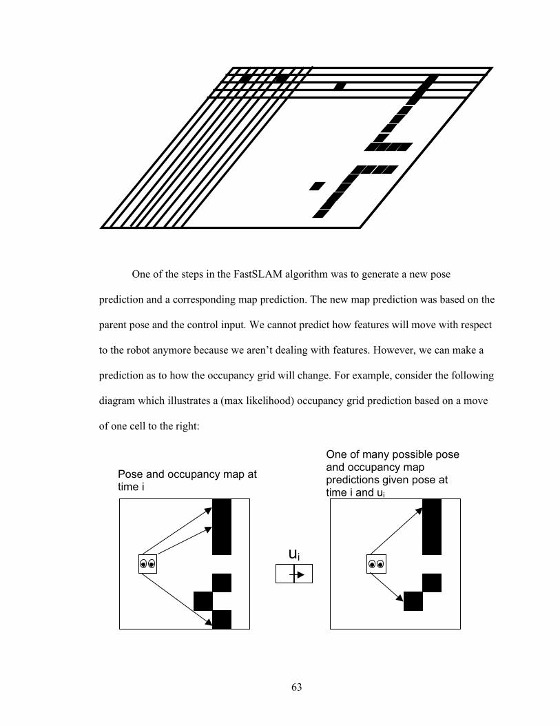
63
One of the steps in the FastSLAM algorithm was to generate a new pose
prediction and a corresponding map prediction. The new map prediction was based on the
parent pose and the control input. We cannot predict how features will move with respect
to the robot anymore because we aren’t dealing with features. However, we can make a
prediction as to how the occupancy grid will change. For example, consider the following
diagram which illustrates a (max likelihood) occupancy grid prediction based on a move
of one cell to the right:
ui
Pose and occupancy map at time i
One of many possible pose and occupancy map predictions given pose at time i and ui
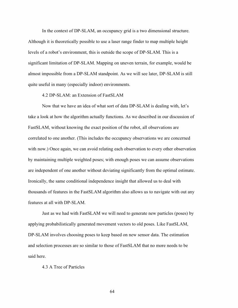
64
In the context of DP-SLAM, an occupancy grid is a two dimensional structure.
Although it is theoretically possible to use a laser range finder to map multiple height
levels of a robot’s environment, this is outside the scope of DP-SLAM. This is a
significant limitation of DP-SLAM. Mapping on uneven terrain, for example, would be
almost impossible from a DP-SLAM standpoint. As we will see later, DP-SLAM is still
quite useful in many (especially indoor) environments.
4.2 DP-SLAM: an Extension of FastSLAM
Now that we have an idea of what sort of data DP-SLAM is dealing with, let’s
take a look at how the algorithm actually functions. As we described in our discussion of
FastSLAM, without knowing the exact position of the robot, all observations are
correlated to one another. (This includes the occupancy observations we are concerned
with now.) Once again, we can avoid relating each observation to every other observation
by maintaining multiple weighted poses; with enough poses we can assume observations
are independent of one another without deviating significantly from the optimal estimate.
Ironically, the same conditional independence insight that allowed us to deal with
thousands of features in the FastSLAM algorithm also allows us to navigate with out any
features at all with DP-SLAM.
Just as we had with FastSLAM we will need to generate new particles (poses) by
applying probabilistically generated movement vectors to old poses. Like FastSLAM,
DP-SLAM involves choosing poses to keep based on new sensor data. The estimation
and selection processes are so similar to those of FastSLAM that no more needs to be
said here.
4.3 A Tree of Particles

65
We claimed earlier that we would keep track of multiple robot poses each with a
unique occupancy grid. This claim is true, but also somewhat misleading; there will be a
unique occupancy grid which corresponds to each particle, but we will not keep track of
those grids explicitly. In a realistic environment we will want large grids to more finely
describe the position of objects and structures. Creating an entire new occupancy grid for
each new particle is generally inefficient. Remember that when we create a new
occupancy grid, it is probabilistically based on a parent grid and a movement vector. In
particular, it should only differ from the parent grid in places which can be observed with
the laser range finder from the new position (Eliazar and Parr [2004]). (We will refer to
the size of the area swept out by the laser as A.) One obvious solution is to only store
discrepancies between the child occupancy grid and the parent occupancy grid. Assuming
that the laser only provides data for a small portion of the entire grid, storing only the
discrepancies between the parent and child node would save a lot of time and space.
Consequently, in DP-SLAM we will maintain a particle ancestry tree to avoid copious
amounts of occupancy grid copying (in contrast to FastSLAM where we just maintained
a fixed size set of particles and forget old particles).
This creates a new problem: the height of the particle ancestry tree will be linear
with respect to the amount of time the algorithm has been running. This means there is no
upper bound on the amount of time it takes to examine a cell in an occupancy grid (as we
might need to search the entire ancestry tree for changes to the particle). We can solve
this problem by carefully defining a method of collapsing certain branches of the tree
(Eliazar and Parr [2004]). Notice that any particle that does not produce any surviving
children is likely a poor pose estimate and can simply be removed; this may cause a
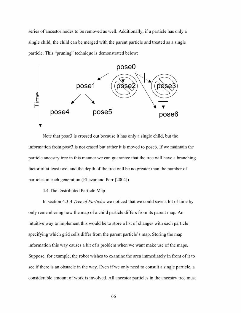
66
series of ancestor nodes to be removed as well. Additionally, if a particle has only a
single child, the child can be merged with the parent particle and treated as a single
particle. This “pruning” technique is demonstrated below:
Note that pose3 is crossed out because it has only a single child, but the
information from pose3 is not erased but rather it is moved to pose6. If we maintain the
particle ancestry tree in this manner we can guarantee that the tree will have a branching
factor of at least two, and the depth of the tree will be no greater than the number of
particles in each generation (Eliazar and Parr [2004]).
4.4 The Distributed Particle Map
In section 4.3 A Tree of Particles we noticed that we could save a lot of time by
only remembering how the map of a child particle differs from its parent map. An
intuitive way to implement this would be to store a list of changes with each particle
specifying which grid cells differ from the parent particle’s map. Storing the map
information this way causes a bit of a problem when we want make use of the maps.
Suppose, for example, the robot wishes to examine the area immediately in front of it to
see if there is an obstacle in the way. Even if we only need to consult a single particle, a
considerable amount of work is involved. All ancestor particles in the ancestry tree must
pose0
pose3 pose2
pose6 pose5 pose4
pose1
Tim
e
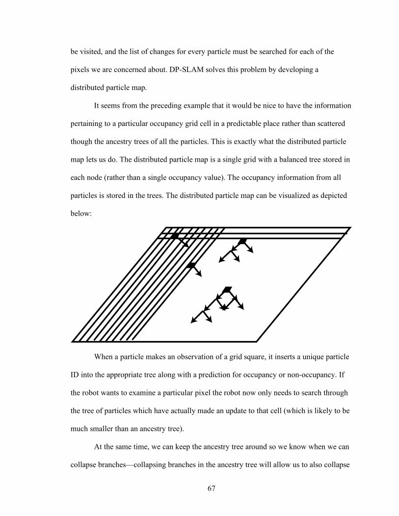
67
be visited, and the list of changes for every particle must be searched for each of the
pixels we are concerned about. DP-SLAM solves this problem by developing a
distributed particle map.
It seems from the preceding example that it would be nice to have the information
pertaining to a particular occupancy grid cell in a predictable place rather than scattered
though the ancestry trees of all the particles. This is exactly what the distributed particle
map lets us do. The distributed particle map is a single grid with a balanced tree stored in
each node (rather than a single occupancy value). The occupancy information from all
particles is stored in the trees. The distributed particle map can be visualized as depicted
below:
When a particle makes an observation of a grid square, it inserts a unique particle
ID into the appropriate tree along with a prediction for occupancy or non-occupancy. If
the robot wants to examine a particular pixel the robot now only needs to search through
the tree of particles which have actually made an update to that cell (which is likely to be
much smaller than an ancestry tree).
At the same time, we can keep the ancestry tree around so we know when we can
collapse branches—collapsing branches in the ancestry tree will allow us to also collapse
68
branches of the distributed particle map’s trees. If a child has no siblings and is therefore
merged with a parent in the ancestry tree, we can first consult the list of particles the child
has changed from its parents map and make the appropriate changes in the distributed
particle grid. (The appropriate changes are to alter the parent’s observations to match the
child’s, and then to remove the child’s observations from the trees in the distributed
particle map.) This bounds the number of objects in each tree to the number of particles
in each generation, and in practice the trees remain much smaller (Eliazar and Parr
[2004]).
4.5 DP-SLAM in Practice
The computational complexity in terms of strict upper bounds for DP-SLAM may
seem larger than we might like. For example, suppose we need to know the prediction
made by a particular particle on a particular grid square. In the worst case, we will need
to search the entire tree at that grid square for all ancestors of the particular particle. We
therefore have a cell access time of O(DlogQ) where D is the height of the ancestry tree
and there are Q particles in each generation. Remember we said that the height of the
ancestry tree, D, was bounded by the number of particles in each generation, Q. In
practice D tends to be approximately O(logQ) (Eliazar and Parr [2004]). The cell access
time is therefore approximately O(log2Q).
To generate a new particle, we need to make A cell accesses from the current
distributed particle map. (Remember, A is the number of cell observations made by a
single pass of the laser.) To produce a new generation of P particles from the last
generation of P particles, A * P total cell accesses are required. Since we just decided
accessing a single cell takes on the order of O(log2Q), the complexity for generating a
69
new set of particles is O(A * P * log2Q). We can expect that the cost of inserting
information into the distributed particle map and maintaining the particle ancestry tree
will have complexity less than or equal to O(A * P * log2Q), so this will ultimately be the
time complexity for an iteration of the DP-SLAM algorithm (Eliazar and Parr [2004]).
In practice, the complexity of DP-SLAM is fast enough to be employed in real-
time (Eliazar and Parr [2004]). Eliazar and Parr implemented DP-SLAM on a small robot
using a resolution of 3 centimeters for the occupancy grid cells, and mapped a 60 meter
corridor using 9000 particles. The time it took to collect data for an iteration of the DP-
SLAM algorithm was approximately equal to the amount of time it would take a 2.4 GHz
computer to perform the computations for the iteration (Eliazar and Parr [2004]). (The
robot’s processor was slightly slower, so some waiting was involved in the actual
experiments at Duke.) DP-SLAM is the only method described in this project which
produces maps which are readily interpretable by humans. The following diagram is the
complete map corresponding to the highest weighted particle of the 9000 total final
generation particles as presented Eliazar and Parr on their original article on DP-SLAM.
(It is illuminating to see the product of running the algorithm in a real world environment
rather than an example of what a map might look like. I have therefore chosen to include
this original diagram produced by the creators of DP-SLAM: Eliazar and Parr. This
diagram in no way represents work done by the author of this thesis. Note that this is the
only diagram in this thesis copied from another source.)
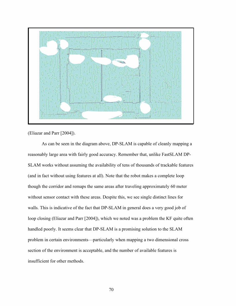
70
(Eliazar and Parr [2004]).
As can be seen in the diagram above, DP-SLAM is capable of cleanly mapping a
reasonably large area with fairly good accuracy. Remember that, unlike FastSLAM DP-
SLAM works without assuming the availability of tens of thousands of trackable features
(and in fact without using features at all). Note that the robot makes a complete loop
though the corridor and remaps the same areas after traveling approximately 60 meter
without sensor contact with these areas. Despite this, we see single distinct lines for
walls. This is indicative of the fact that DP-SLAM in general does a very good job of
loop closing (Eliazar and Parr [2004]), which we noted was a problem the KF quite often
handled poorly. It seems clear that DP-SLAM is a promising solution to the SLAM
problem in certain environments—particularly when mapping a two dimensional cross
section of the environment is acceptable, and the number of available features is
insufficient for other methods.
71
5 Conclusion
5.1 The SLAM Problem Revisited
We began our discussion in the first chapter by establishing what the SLAM
problem is on an intuitive level, and by discussing what a solution to the SLAM problem
would accomplish. In short, the SLAM problem is tough to solve or even understand
fully, but the closer we get to solving it the more we open the door to a truly autonomous
robot. To better understand the SLAM problem, we first broke the SLAM problem down
into the component problems (localization and mapping on their own), and we discovered
each could be solved without too much trouble. The problem is, in order to localize we
need to start with an error free map, and to map we need to be able to localize. This is
what motivated us to consider the first solution to the SLAM problem, the Kalman Filter.
5.2 Solutions Revisited
In the Kalman Filter we found a solution that could take advantage of all available
data statistically minimize the total squared error in our state prediction. The KF
accomplishes this task for us by maintaining a state prediction and a covariance matrix
containing a confidence value for every binary relationship in the environment. We
noticed the KF specified how each observation could be used to update all feature
predictions, and all covariance matrix values. Also, we noticed that the state prediction
and covariance matrix had a fixed size independent of the number of iterations of the
filter. Consequently, the KF allows us to map for as long as we want without increasing
the time to run each iteration. It is safe to say that if there are approximately 200 features
we wish to map, a Kalman Filter will be the correct method to use.
72
While the Kalman Filter is optimal in the sense that it yields a least squares
prediction, it cannot always produce this prediction in real time. The problem is
maintaining the covariance matrix which is quadratic in size with respect to the number
of features. We dealt with this problem in our discussion of FastSLAM. FastSLAM
approaches SLAM from a Bayesian perspective and draws upon the insight that
observations are conditionally independent of one another given the true robot pose.
Errors in robot pose are accounted for by maintaining a set of poses called particles. Our
discussion of the KF came in particularly handy here because FastSLAM uses simple
Kalman Filters (just like the one we developed at the beginning of chapter 2) to update
each feature prediction for each particle. This allows for an approximation of the optimal
estimate while at the same time making it possible to take many more features into
account. FastSLAM often outperforms KF based approaches despite being non-optimal
because so many more features can be utilized in a given amount of time.
We also considered the reverse situation, in which there are not enough features to
effectively employ FastSLAM or Kalman Filter based approaches. DP-SLAM uses an
entirely different way of representing maps. Laser range finders are employed to create
occupancy grids rather than vectors of features. The same insight (conditional
independence of observations given robot pose) we discovered in our discussion of
FastSLAM is utilized to eliminate the need to correlate observations. Once again,
maintaining multiple particles minimizes the effect of errors in the robot pose, and each
particle has a corresponding map. The overhead of maintaining multiple occupancy grids
is minimized by keeping an ancestry tree and only storing discrepancies between a child
an parent. We improved the efficiency in retrieving the occupancy information
73
corresponding to particular grid cell by distributing the information from all particles
over a single particle map. This distributed particle map stores all the information
regarding each grid square in a balanced tree for quick lookup.
To summarize: In environments where a couple hundred features are available
and it is crucial that the best possible estimate be made for each feature, Kalman Filter
approaches outperform the other two. Where tens of thousands of features are available,
FastSLAM is usually a better solution. DP-SLAM often excels on level terrain without
any features at all. The three solutions we have considered here together represent a good
practical solution to the SLAM problem in an environment with any number of features.
5.3 Connections Between Solutions
Earlier in this thesis it was claimed that we would see how these three approaches
build off and motivate one another. The basis for this claim should now be clear. It was
the high computational complexity of the Kalman Filter which led us to consider a way
of approximating the optimal solution without keeping track of the covariance matrix, i.e.
FastSLAM.
FastSLAM in turn avoids using the covariance matrix by maintaining multiple
pose particles. Not only did the KF motivate FastSLAM, Kalman Filters are actually
utilized by FastSLAM to estimate feature locations.
Finally, we realized the motivation for DP-SLAM was the fact that both the KF
and FastSLAM require many trackable features which are not always available. DP-
SLAM utilizes multiple pose particles (just as we saw in FastSLAM) to improve
accuracy.
5.4 Future Work
74
An extension of the work done in this thesis might be to combine the three
algorithms described in this thesis in a way that yields more robust performance. There is
no reason a robot would never travel from an environment with many available features
to one without features. Additionally a robot might be able to observe both areas with
features and areas without from a single location. It seems that if a robot were able to use
both a laser range finder to employ DP-SLAM and a camera to employ FastSLAM then it
would be better prepared to handle more diverse environments. SLAM methods
combining data from camera sensors and laser range finders were considered before
FastSLAM or DP-SLAM were developed and these yielded greater accuracy than other
contemporary methods (Castellanos, Neira, Tardos, [2001]). It may be that combining the
new algorithms we have discussed could yield even better results.
5.5 Concluding Remarks
The time has come to conclude our discussion of the SLAM problem and the
promising solutions presented in this thesis. It should now be clear that there is no one
right answer to the SLAM problem. There are different ways of collecting data, and
different ways of using the data after it is collected. Different environments lend
themselves to different approaches, and each of the algorithms presented in this thesis
have their place.
75
Bibliography
Castellanos, J. A., Neira, J., and Tardos, J. D. Limits to the consistencyof the EKF-based SLAM. In Intelligent Autonomous Vehicles (IAV-2004) (Lisboa, PT, July 2004), M. I. Ribeiro and J. Santos-Victor, Eds., IFAC/EURON, IFAC/Elsevier.
Castellanos, J. A., Neira, J., and Tardós, J. D. Multisensor fusion for simultaneous
localization and map building. IEEE Trans on Robotics and Automation 17, 6 (December 2001), 908-914.
Csorba, M. Simultaneous Localisation and Mapping. PhD thesis, Univ of Oxford, 1997. Durrant-Whyte, Hugh “Localization, Mapping, and the Simultaneous Localization and Mapping Problem.” Australian Center for Field Robotics. Sydney. 2002. Eliazar, A., and Parr, R. Dp-slam: Fast, robust simulataneous localization and mapping
without predetermined landmarks. In 18th IJCAI (Acapulco, August 2003). Hähnel, D., Burgard, W., Fox, D., and Thrun, S. A highly efficient fastslam algorithm for
generating cyclic maps of large-scale environments from raw laser range measurements. In IROS (Las Vegas (USA), 2003), IEEE/RSJ.
Huang, Tim “Machine Learning.” Middlebury College. Middlebury. 2005. Maybeck, Peter S. Stochastic, Models, Estimation, and Control. New York: Academic Press, 1979. Montemerlo, M., Thrun, S., Koller, D., and Wegbreit, B. Fastslam: A factored solution to
the simultaneous localization and mapping problem. In AAAI-2002 (Vancouver, BC, July 2002).
Scharstein, Daniel “Computer Vision.” Middlebury College. Middlebury. 2006. Scharstein, Daniel “Artificial Intellegence.” Middlebury College. Middlebury. 2005. Stachniss, C., and Burgard, W. Exploration with active loop-closing for fastslam. In IROS
(Sendai (Japan), Sep 2004), IEEE/RSJ. Trucco., and Alessandro Verri. Introductory Techniques for 3-D Computer Vision. : Prentice Hall, 1998. Welch, Greg, and Bishop, Gary. “An Introduction to the Kalman Filter.” Technical Documents 95041 (2006). 15 May. 2007. <http://www.cs.unc.edu/~welch/media/pdf/kalman_intro.pdf>.
Recommended


![Decoupled Localization and Sensing ... - vision.cornell.edu · with vision-based Simultaneous Localization and Mapping (SLAM) (e.g., [10,11]) or ICP-based tracking with RGBD input](https://img.pdfslide.us/doc/110x75/5f0e8cc37e708231d43fc81b/decoupled-localization-and-sensing-with-vision-based-simultaneous-localization.jpg)