An Introduction to Real-Time Operating Systems and Schedulability Analysis
Marco Di NataleScuola Superiore S. Anna
Outline
• Background on Operating Systems Theory• An Introduction to RT Systems• Model-based development of Embedded RT systems
– the RTOS in the platform-based design
• Scheduling and Resource Management• Schedulability Analysis and Priority Inversion• Schedulability Analysis and Priority Inversion
– The Mars Pathfinder case
• Implementation issues and standards– OSEK
Credits
• Paolo Gai (Evidence S.r.l.) – slides 68 to 70, 147 to 177• Giuseppe Lipari (Scuola Superiore S. Anna) – slides 189 to 235• Manas Saksena (TimeSys) – examples in slides 93 and 108• From Mathworks Simulink and RTW manuals – 133-134-138
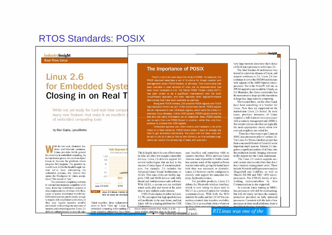
RTOS Standards: POSIX
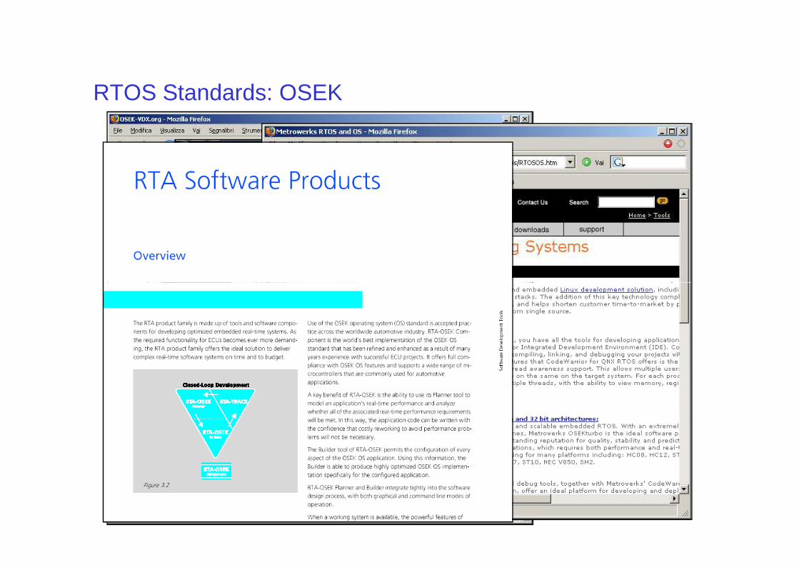
RTOS Standards: OSEK
Definitions of Real-time system
• Interactions between the system and the environment (environment dynamics).
• Time instant when the system produces its results (performs an action).
• A real-time operating system is an interactive system that maintains an ongoing relationship with an asynchronous environment i.e. an environment that progresses irrespective of the RTSthe RTS
• A real-time system responds in a (timely) predictable way to (un)predictable external stimuli arrival.
• (Open, Modular, Architecture Control user group - OMAC): a hard real-time system is a system that would fail if its timing requirements were not met; a soft real-time system can tolerate significant variations in the delivery of operating system services like interrupts, timers, and scheduling.
• In real-time computing correctness depends not only on the correctness of the logical result of the computation but also on the result delivery time (timing constraints).
Timing constraints
• Where do they come from ?• From system specifications (design choices?)
Specifications
Software design
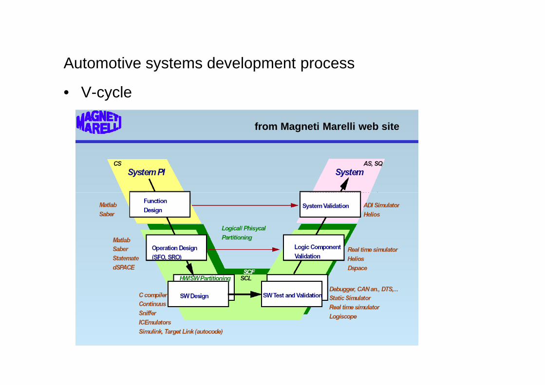
Automotive systems development process
• V-cycle
from Magneti Marelli web site
Control algorithmdesign
Control designsign-off
Software design
Functionaltesting
Software designsign-off
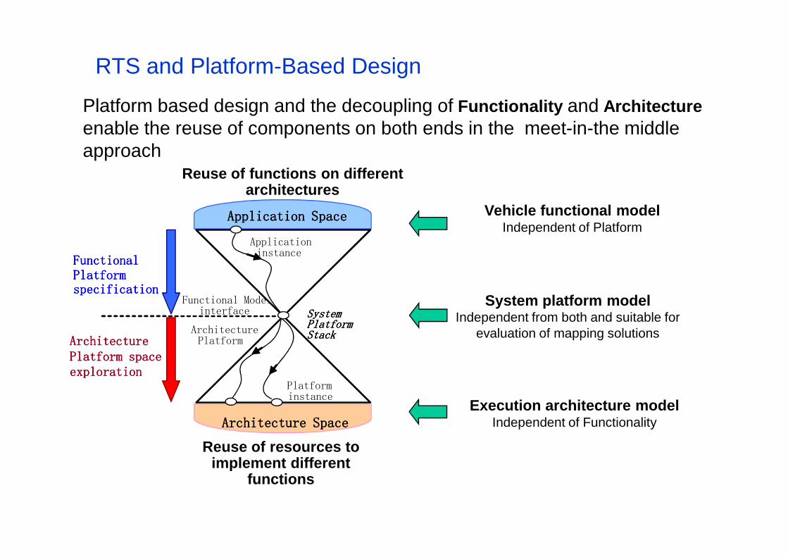
RTS and Platform-Based Design
Platform based design and the decoupling of Functionality and Architecture enable the reuse of components on both ends in the meet-in-the middle approach
Functional Functional Functional Functional Platform Platform Platform Platform
Application instance
Vehicle functional modelIndependent of Platform
Reuse of functions on different architectures
Application SpaceApplication SpaceApplication SpaceApplication Space
Architecture SpaceArchitecture SpaceArchitecture SpaceArchitecture Space
Platform Platform Platform Platform specificationspecificationspecificationspecification
ArchitectureArchitectureArchitectureArchitecturePlatform space Platform space Platform space Platform space explorationexplorationexplorationexploration
Functional Model interface
Platforminstance
Architecture Platform
SystemSystemSystemSystemPlatformPlatformPlatformPlatformStackStackStackStack
Reuse of resources to implement different
functions
Execution architecture modelIndependent of Functionality
System platform modelIndependent from both and suitable for
evaluation of mapping solutions
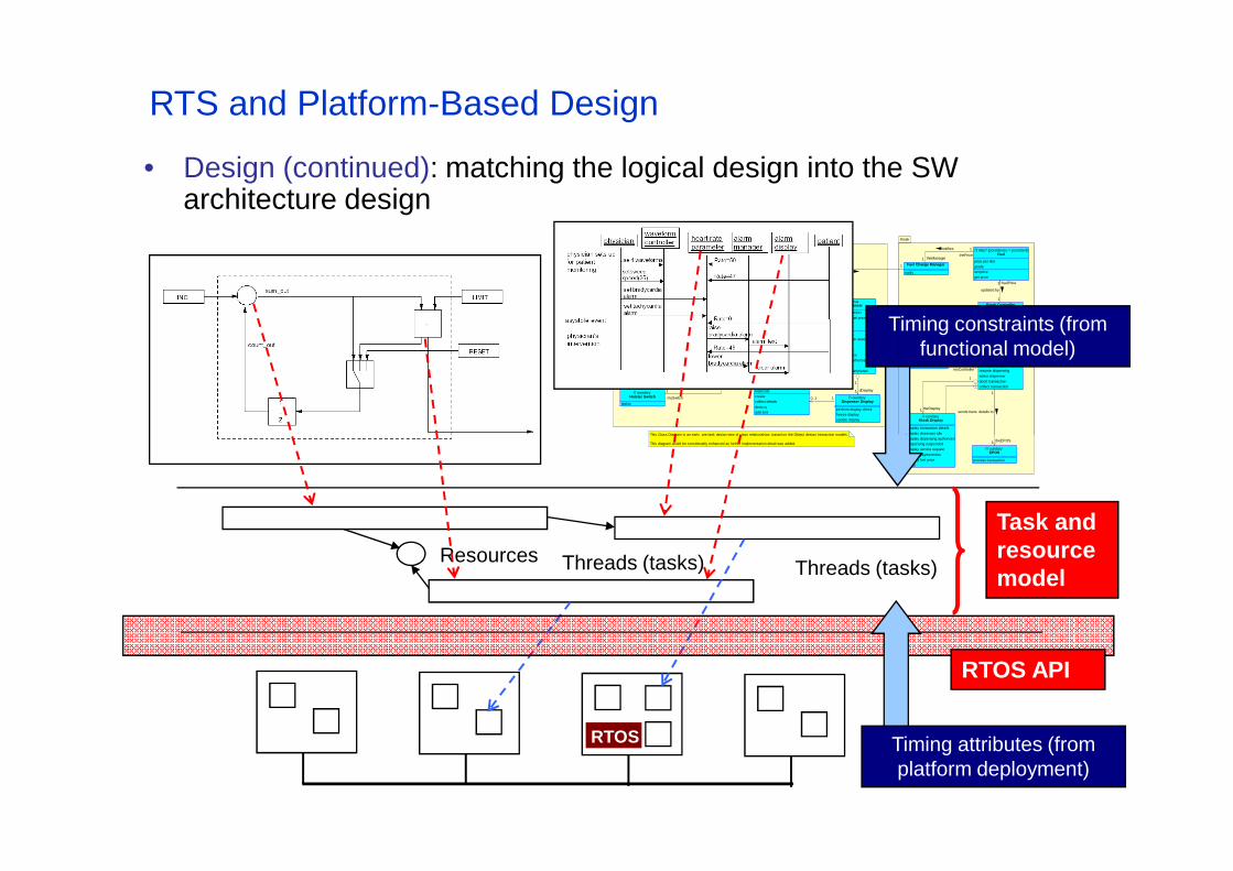
• Design (continued): matching the logical design into the SW architecture design
Dispenser
玝oundary�Valve
statusopenclose
玝oundary�Holster Switch
status
玝oundary�Flowmeter
count
玝oundary�Motor
statusstop
start
玜uxiliary? {semantics = controls EH Unit}EH Unit
activeEH idnozzle removeddispensing authorised
haltresumefuel pulsenozzle replaced
玣ocus�Dispenser
dispenser number
transaction fuel priceactive EH idfuel_gradeabort
get transaction detailshaltget fuel pricerequest servicedispensing authorised
resumedispensing completed
玝oundary�Dispenser Display
perform display checkfreeze displayupdate display
玡ntity? {persistence = transitory}Fuel Transaction
litres dispensed
price per litretotal costcreatecollect details
destroyadd 5ml
玡ntity? {persistence = persistent}Fuel Observer
price per litregrade
set priceget price
Kiosk
玡ntity? {persistence = persistent}Fuel
price per litregradeset priceget price
Kiosk Controller
fuel pricefuel amountfuel grade
transaction amountselect gradenew price informationpayment duedispensing authorized
display fuel pricerequest servicehalt dispensingresume dispensing
select dispenserabort transactioncollect transaction
玝oundary�Keyboard Unit
玝oundary�Kiosk Display
display transaction details
display dispenser idle
Fuel Change Manager
notify
1
1fuel type available at
3
1
gets price fromtheObserver
1
1
myMotor
1
3
updated by
fuelPrice
3 1
myDispensermyEHUnits
0..1 1active
theDispenseractiveEH
1
sends trans. details to
1
1myEH
mySwitch
1
1
myMeter
0..1 1
1
1
dDisplay
11..16 controlled by
aDispenser theKiosk
1 1
myController
1
1
theDisplay
2 1
myValves
11..16
updated by
1
1
notifies
theManagerthePrice
This Class Diagram is an early, pre-task design view of class relationships, based on the Object design interaction models.
the 'active' EH Unit is one of the aggregate EH Units of the Dispenser Timing constraints (from
functional model)
RTS and Platform-Based Design
玝oundary�EPOS
process transaction
display dispensing authoriseddispensing suspendeddisplay service request
display payment duedisplay fuel priceclear
玝oundary�EPOS
process transaction
display dispensing authoriseddispensing suspendeddisplay service request
display payment duedisplay fuel priceclear
1 theEPOS
This Class Diagram is an early, pre-task design view of class relationships, based on the Object design interaction models.
This diagram would be considerably enhanced as further implementation detail was added.
RTOS
Threads (tasks)Threads (tasks)Resources
RTOS API
Task and resource model
Timing attributes (from platform deployment)
An introduction to Real-Time scheduling
• Application of schedulability theory (worst case timing analysis and scheduling algorithms)
• for the development of scheduling and resource management algorithms inside the RTOS, driving the development of efficient (in the worst case) and predictable OS mechanisms (and methods for accessing OS data OS mechanisms (and methods for accessing OS data structures)
• for the evaluation and later verification of the design of embedded systems with timing constraints and possibly for the synthesis of an efficient implementation of an embedded system (with timing constraints) model – synthesis of the RTOS
Real-time scheduling
• Assignment of system resources to the software threads• System resources
– pyhsical: CPU, network, I/O channels– logical: shared memory, shared mailboxes, logical channels
• Typical operating system problem• In order to study real-time scheduling policies we need a model
for representing– abstract entities
• actions, • events, • time, timing attributes and constraints
– design entities• units of computation• mode of computation• resources
Classification of RT Systems
• Based on input– time-driven: continuous (synchronous) input– event-driven: discontinuous (asynchronous) input
• Based on criticality of timing constraints– hard RT systems: response of the system within the timing
constraints is crucial for correct behavior– soft RT systems: response of the system within the timing
constraints increases the value of the systemconstraints increases the value of the system• Based on the nature of the RT load:
– static: predefined, constant and deterministic load– dynamic: variable (non deterministic) load
• real world systems exhibit a combination of these characteristics
Classification of RT Systems: criticality
• Typical Hard real time systems– Aircraft, Automotive– Airport landing services– Nuclear Power Stations– Chemical Plants– Life support systems
• Typical Soft real time systems• Typical Soft real time systems– Multimedia– Interactive video games

Classification of RT Systems: criticality
• Hard, Soft and Firm type
valueHard type value
Firm typevalue
Soft type
deadline
-∞
time
deadline
0 time
deadline
time
Classification of RT Systems: Input-based
• Event-Triggered vs. Time-Triggered models• Time triggered
– Strictly periodic activities (periodic events)
• Event triggered– activities are triggered by external or internal asynchronous
events, not necessarily related to a periodic time reference
Classification of RT Systems: Input-based
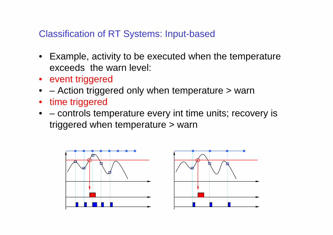
• Example, activity to be executed when the temperature exceeds the warn level:
• event triggered• – Action triggered only when temperature > warn• time triggered• – controls temperature every int time units; recovery is • – controls temperature every int time units; recovery is
triggered when temperature > warn
Classification of RT Systems: Input-based
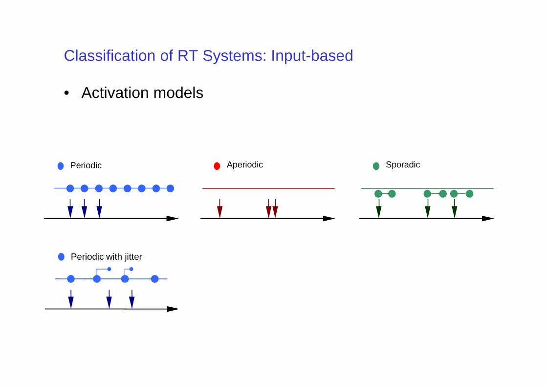
• Activation models
Periodic Aperiodic Sporadic
Periodic with jitter
Modeling Real-time systems
• We need to identify (in the specification and design phase)– Events and Actions (System responses).
• Some temporal constraints are explicitly expressed as a results of system analysis
– “The alarm must be delivered within 2s from the time instant a dangerous situation is detected”
• More often, timing constraints are hidden behind sentences that are apparently not related to time …
– And are the result of design choices ….
Modeling Real-time systems
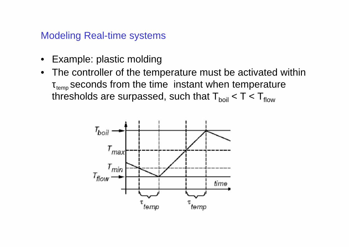
• Example: plastic molding• The controller of the temperature must be activated within
τtemp seconds from the time instant when temperature thresholds are surpassed, such that Tboil < T < Tflow
Modeling Real-time systems
• … the injector must be shut down no more than τinj
seconds after receiving the end-run signals A or B such that vinjτinj < δ
Modeling Real-time systems
• (UML profile, alternate notation)
{0 ms}
InstanceA : InstanceB :
helloMsg{0 ms}
{11 ms}
{10.2 ms}
{4.7 ms}
{2 ms}
{1.5 ms}
ackMsg
2.7 ms
Modeling Real-time systems
• What type of timing constraints are in a Simulink diagram
Scheduling of Real-time systems
• What are the key concepts for real-time systems?– Schedulable entities (threads)– Shared resources (physical – HW / logical)– Resource handlers (RTOS)
• Defined in the design of the Architectural level
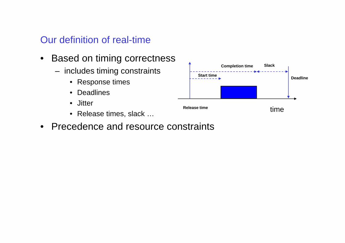
Our definition of real-time
• Based on timing correctness– includes timing constraints
• Response times • Deadlines• Jitter• Release times, slack …
• Precedence and resource constraints
timeRelease time
Start time
Completion time
Deadline
Slack
• Precedence and resource constraints
Real-time systems: handling timing constraints
• Real Time = the fastest possible implementation dictated by technology and/or budget constraints ?
• “the fastest possible response is desired. But, like the cruise control algorithm, fastest is not necessarily best, because it is also desirable to keep the cost of parts down by using small microcontrollers. What is important is for the application requirements to specify a worst-case important is for the application requirements to specify a worst-case response time. The hardware and software is then designed to meet those specifications“
• “Embedded systems are usually constructed with the least powerful computer that can meet the performance requirements. Marketing and sale concerns push for using smaller processors and less memory reducing the so-called recurring costs”
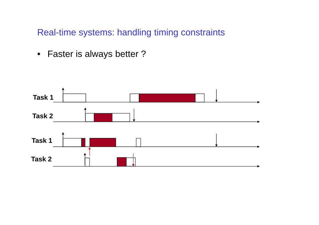
Real-time systems: handling timing constraints
• Faster is always better ?
Task 1
Task 2Task 2
Task 1
Task 2
Real-time systems: handling timing constraints
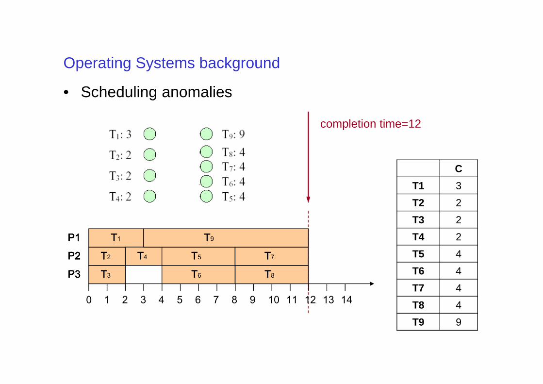
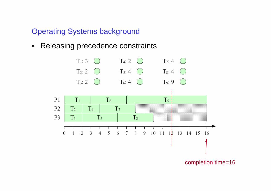
• Scheduling anomalies [Richards]• The response time of a task in a real-time system may
increase if– the execution time of some of the tasks is reduced– precedence constraints are removed from the specifications– additional resources (processors) are added to the system ...
Operating Systems background
• Scheduling anomalies
completion time=12
C
T1 3
T2 2
T3 2
T4 2
T5 4
T6 4
T7 4
T8 4
T9 9
0 1 2 3 4 5 6 7 8 9 10 11 12 13 14
P3P3P3P3 TTTT3
P2P2P2P2 TTTT2
P1P1P1P1 TTTT1
TTTT4 TTTT5
TTTT6 TTTT8
TTTT7
TTTT9
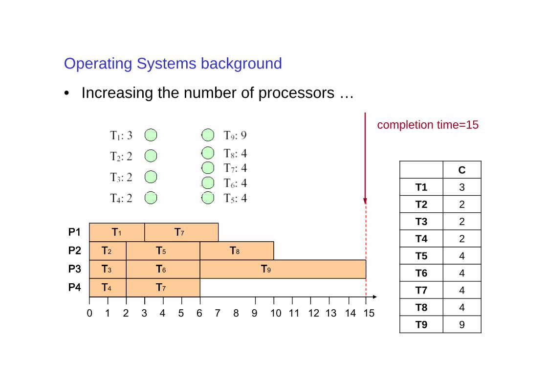
Operating Systems background
• Increasing the number of processors …
completion time=15
C
T1 3
T2 2
T3 2
T4 2
T5 4
T6 4
T7 4
T8 4
T9 90 1 2 3 4 5 6 7 8 9 10 11 12 13 14
P3P3P3P3 TTTT3
P2P2P2P2 TTTT2
P1P1P1P1 TTTT1
TTTT5
TTTT6
TTTT8
TTTT7
TTTT9
P4P4P4P4 TTTT4 TTTT7
15
A typical solution: cyclic scheduler
• Used for now 40 years in industrial practice• military• navigation• monitoring• control …
• Examples• space shuttle• space shuttle• Boeing 777• code generated by Mathworks embedded coder (single task
mode)
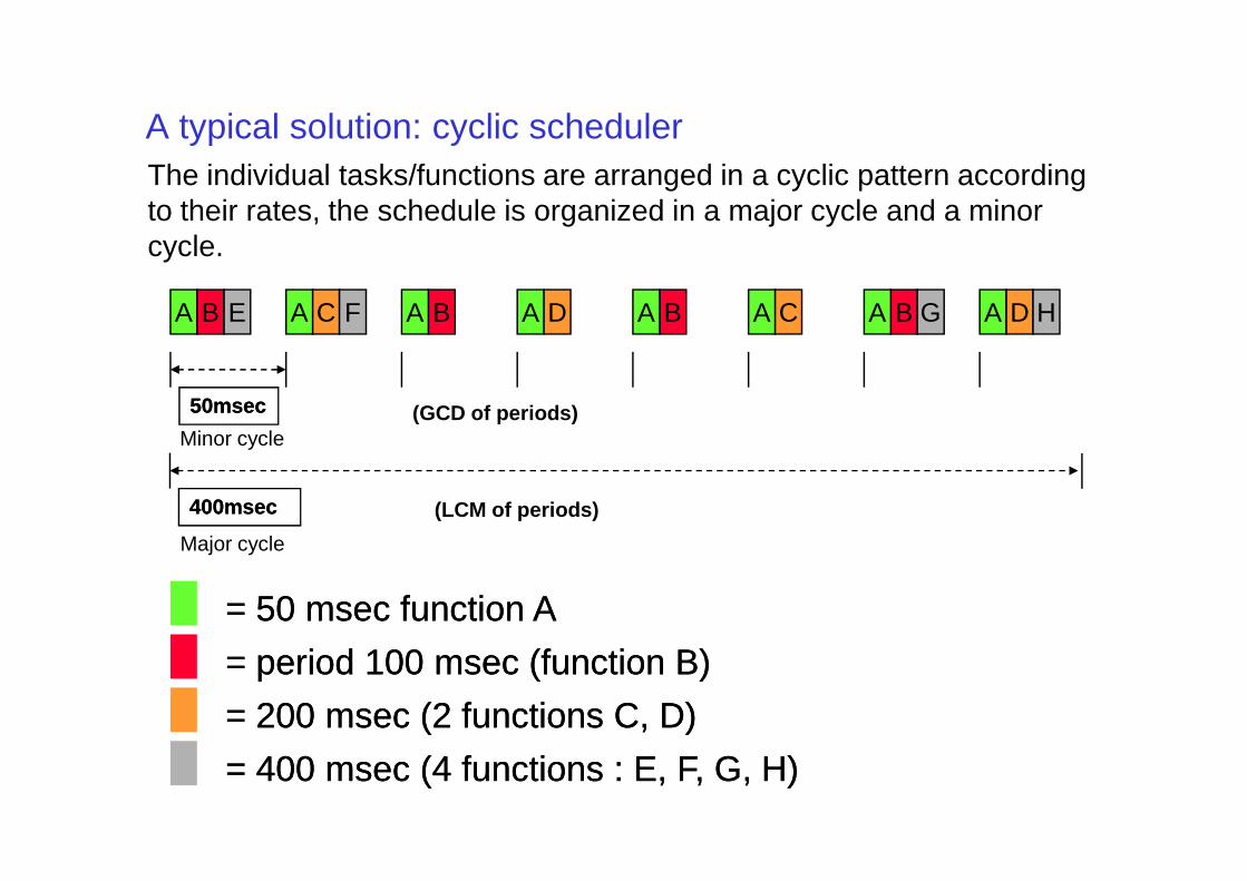
A typical solution: cyclic schedulerThe individual tasks/functions are arranged in a cyclic pattern according to their rates, the schedule is organized in a major cycle and a minor cycle.
B B BA A A AA A A AC D C DE F G H
50msec50msec
Minor cycle(GCD of periods)
B
= 50 msec function A= 50 msec function A
= period 100 msec (function B)= period 100 msec (function B)
= 200 msec (2 functions C, D)= 200 msec (2 functions C, D)
= 400 msec (4 functions : E, F, G, H)= 400 msec (4 functions : E, F, G, H)
Minor cycle
Major cycle
400msec400msec (LCM of periods)
A typical solution: cyclic scheduler
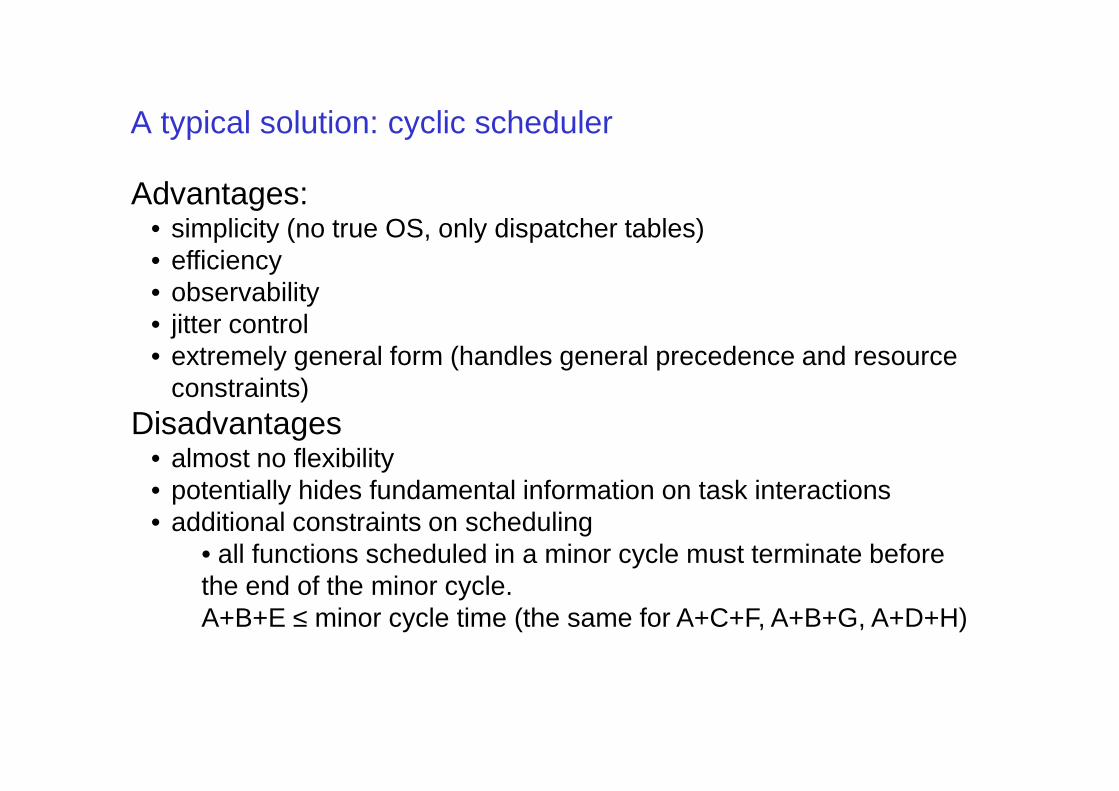
Advantages:• simplicity (no true OS, only dispatcher tables)• efficiency• observability• jitter control• extremely general form (handles general precedence and resource
constraints)constraints)Disadvantages
• almost no flexibility• potentially hides fundamental information on task interactions• additional constraints on scheduling
• all functions scheduled in a minor cycle must terminate before the end of the minor cycle.A+B+E ≤ minor cycle time (the same for A+C+F, A+B+G, A+D+H)
Problems with cyclic schedulers
• Solution is customized upon the specific task set– a different set, even if obtained incrementally, requires a completely
different solution
• Race conditions may be “hidden” by the scheduling solution– see the shared resource section
– problems due to non-protected concurrent accesses to shared resources may suddenly show up in a new solutionresources may suddenly show up in a new solution
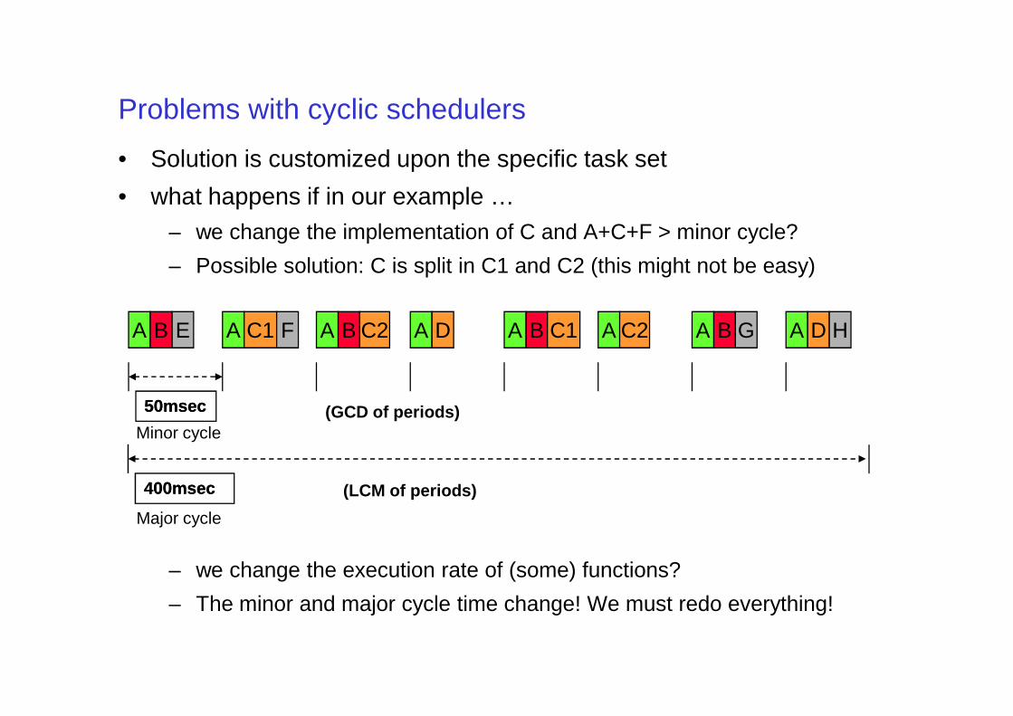
Problems with cyclic schedulers
• Solution is customized upon the specific task set
• what happens if in our example … – we change the implementation of C and A+C+F > minor cycle?
– Possible solution: C is split in C1 and C2 (this might not be easy)
B B BA A A AA A A AC1 D DE F G HB C2 C1 C2
– we change the execution rate of (some) functions?
– The minor and major cycle time change! We must redo everything!
50msec50msec
Minor cycle
Major cycle
400msec400msec (LCM of periods)
(GCD of periods)
From cyclic schedulers (Time triggered systems) to Priority-based scheduling• Periodic timer:
– once initialized send periodic TimeEvents at the appropriate time
instants (minor cycle time) until explicitly stopped or deleted
• Threads exclusively activated by periodic timers are periodic
tasks
– scheduled according to a fixed priority policy– scheduled according to a fixed priority policy
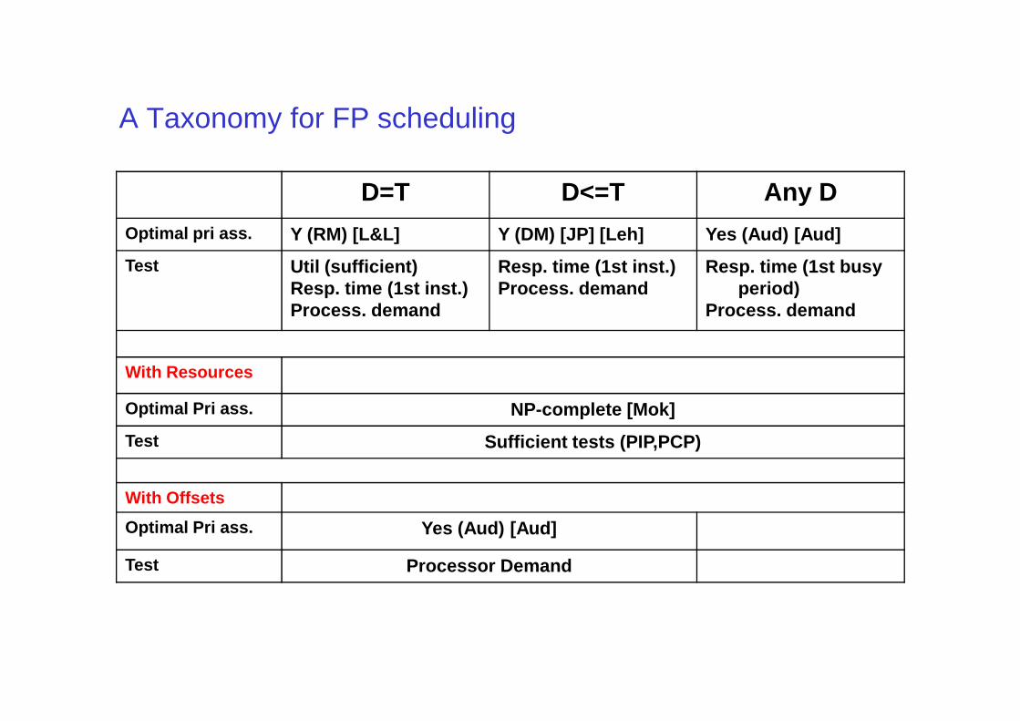
A Taxonomy for FP scheduling
D=T D<=T Any D
Optimal pri ass. Y (RM) [L&L] Y (DM) [JP] [Leh] Yes (Aud) [Aud]
Test Util (sufficient)Resp. time (1st inst.)Process. demand
Resp. time (1st inst.)Process. demand
Resp. time (1st busy period)
Process. demand
With Resources
Optimal Pri ass. NP-complete [Mok]
Test Sufficient tests (PIP,PCP)
With Offsets
Optimal Pri ass. Yes (Aud) [Aud]
Test Processor Demand
Case 1: Independent periodic tasks
• Activation events are periodic (period=T), • Deadlines are timing contraints on the execution of tasks (D=T)
– evey task instance must be completed before the next instance– (no need to provide queues (buffers) for activation events)
• tasks are independent– the execution of a task does not depend upon the execution
(completion) of another task– periods may be correlated– periods may be correlated
• The execution time of each task is constant– approximated with the worst case execution time
Task set
• n indipendent tasks τ1, τ2, … τn
• Task periods T1, T2, ... Tn
– the activation rate of τi is 1/Ti
• Execution times are C1, C2, ... Cn
Scheduling algorithm
• Rules dictating the task that needs to be executed on the CPU at each time instant
• preemptive & priority driven– task have priorities
• statically (design time) assigned– at each time the highest priority task is executed
• if a higher piority task becomes ready, the execution of the • if a higher piority task becomes ready, the execution of the running task is interrupted and the CPU given to the new task
• In this case, scheduling algorithm = priority assignment + priority queue management
Priority-based scheduling
• Static (fixed priorities)• as opposed to ... Dynamic
– the priority of each task instance may be different from the priority of other instances (of the same task)
Definitions ...
• Deadline of a task - latest possible completion time and time instant of the next activation
• Time Overflow when a task completes after the deadline• A scheduling algorithm is feasible if tasks can be
scheduled without overflow• Critical instant of a task = time instant t such that, if the • Critical instant of a task = time instant t0 such that, if the
task instance is released in t0, it has the worst possible response (completion) time (Critical instant of the system)
• Critical time zone time interval between the critical instant and the response (completion) of the task instance
Critical instant for fixed priorities
• Theorem 1: the critical instant for each task is when the task instance is released together with (at the same time) all the other higher priority instances
• The critical instant may be used to check if a priority assignment results in a feasible scheduling– if all requests at the critical instant complete before their – if all requests at the critical instant complete before their
deadlines
Example
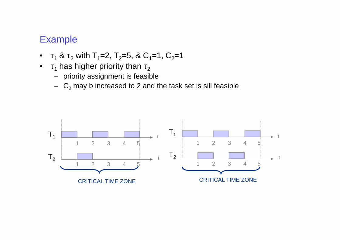
• τ1 & τ2 with T1=2, T2=5, & C1=1, C2=1• τ1 has higher priority than τ2
– priority assignment is feasible– C2 may b increased to 2 and the task set is sill feasible
T1
T2
1 2 3 4 5
1 2 3 4 5
t
t
1 2 3 4 5
1 2 3 4 5
t
t
T1
T2
CRITICAL TIME ZONE CRITICAL TIME ZONE
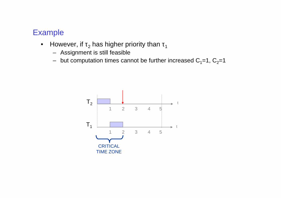
Example• However, if τ2 has higher priority than τ1
– Assignment is still feasible– but computation times cannot be further increased C1=1, C2=1
T
T1
T2
1 2 3 4 5
1 2 3 4 5
t
t
CRITICALTIME ZONE
Rate Monotonic
• Priority assignment rule Rate-Monotonic (RM) • Assign priorities according to the activation rates (indipendently
from computation times)– higher priority for higher rate tasks (hence the name rate monotonic)
• RM is optimal (among all possible staic priority assignments)• Theorem 2: if the RM algorithm does not produce a feasible
schedule, then there is no fixed priority assignment that can schedule, then there is no fixed priority assignment that can possibly produce a feasible schedule
A priori guarantees
• Understanding at design time if the system is schedulable
• different methods– utilization based– based on completion time– based on processor demand– based on processor demand
Processor Utilization
• Processor Utilization Factor: fraction of processor time spent in executing the task set
• i.e. 1 - fraction of time processor is idle
• For n tasks, τ1, τ2, … τn the utilization factor U is
U = C1/T1 + C2/T2 + … + Cn/Tn
• U can be improved by increasing Ci’s or decreasing Ti’s as long as tasks continue to satisfy their deadlines at their critical instants
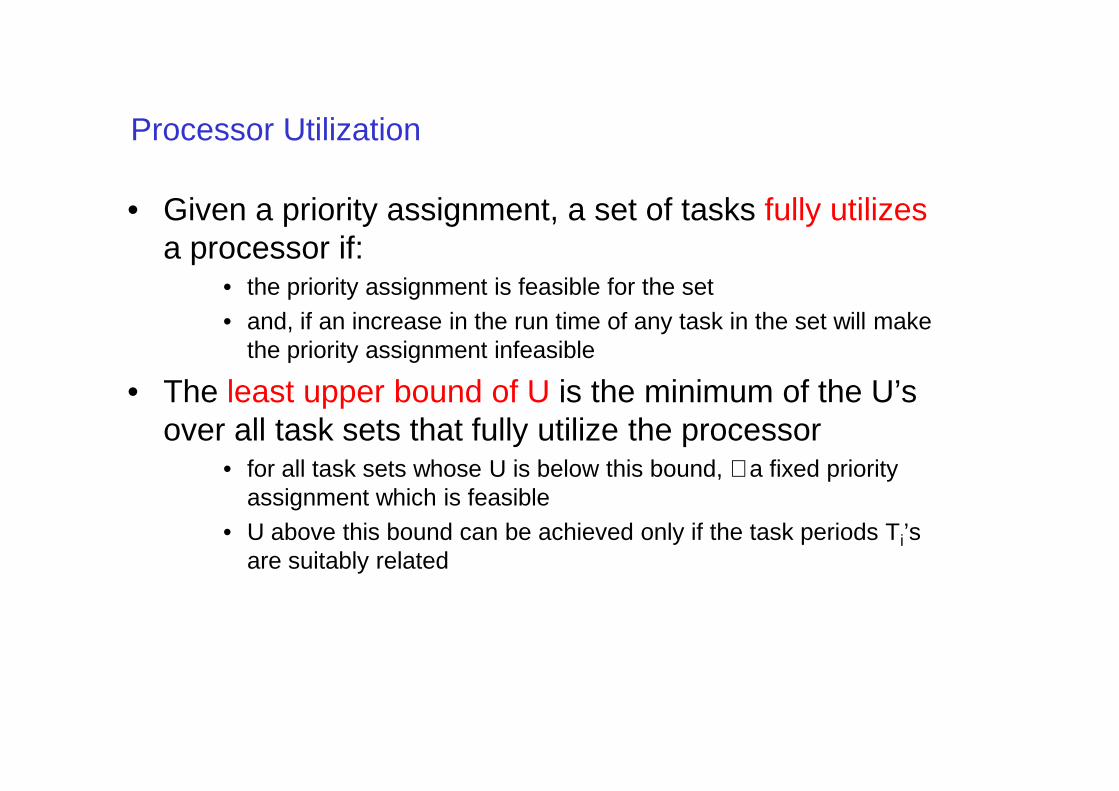
Processor Utilization
• Given a priority assignment, a set of tasks fully utilizesa processor if:
• the priority assignment is feasible for the set• and, if an increase in the run time of any task in the set will make
the priority assignment infeasible
• The least upper bound of U is the minimum of the U’s • The least upper bound of U is the minimum of the U’s over all task sets that fully utilize the processor
• for all task sets whose U is below this bound, ∃ a fixed priority assignment which is feasible
• U above this bound can be achieved only if the task periods Ti’s are suitably related
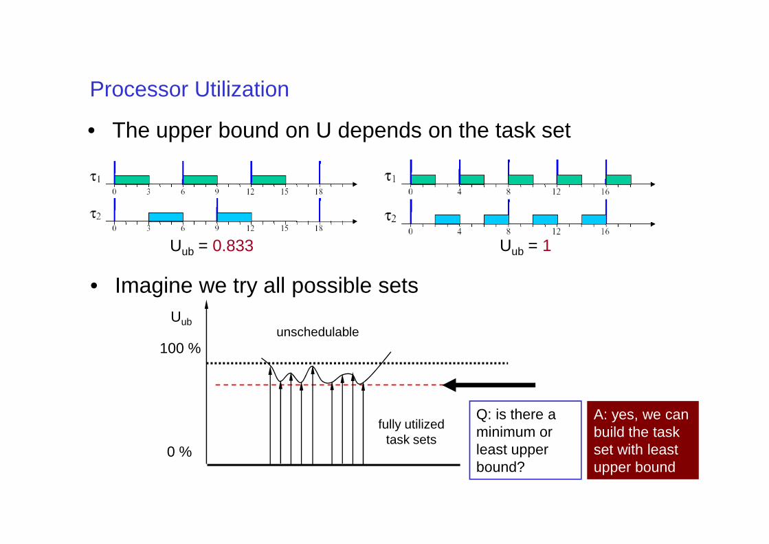
Processor Utilization
• The upper bound on U depends on the task set
Uub = 0.833 Uub = 1
• Imagine we try all possible setsUub
100 %
0 %
fully utilizedtask sets
unschedulable
Q: is there a minimum or least upper bound?
A: yes, we can build the task set with least upper bound
Processor Utilization for Rate-Monotonic
• RM priority assignment is optimal• for a given task set, the U achieved by RM priority
assignment is ≥ the U for any other priority assignment
• the least upper bound of U = the minimum Uub for RM priority assignment over all possible T’s and all C’s priority assignment over all possible T’s and all C’s for the tasks
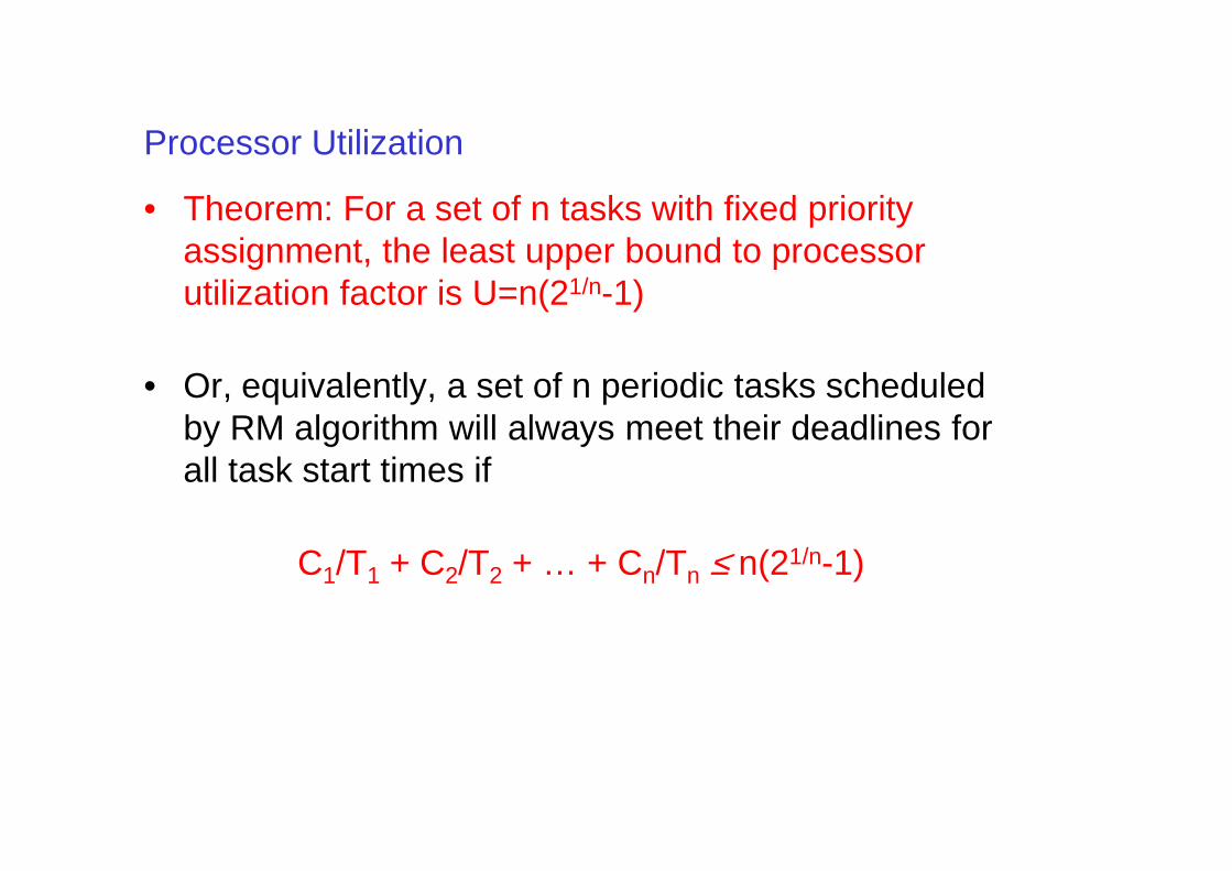
Processor Utilization
• Theorem: For a set of n tasks with fixed priority assignment, the least upper bound to processor utilization factor is U=n(21/n-1)
• Or, equivalently, a set of n periodic tasks scheduled by RM algorithm will always meet their deadlines for by RM algorithm will always meet their deadlines for all task start times if
C1/T1 + C2/T2 + … + Cn/Tn ≤ n(21/n-1)
Processor Utilization
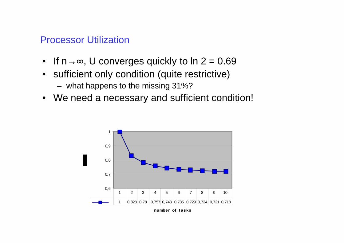
• If n→∞, U converges quickly to ln 2 = 0.69• sufficient only condition (quite restrictive)
– what happens to the missing 31%?
• We need a necessary and sufficient condition!
0,6
0,7
0,8
0,9
1
number of t asks
1 0,828 0,78 0,757 0,743 0,735 0,729 0,724 0,721 0,718
1 2 3 4 5 6 7 8 9 10
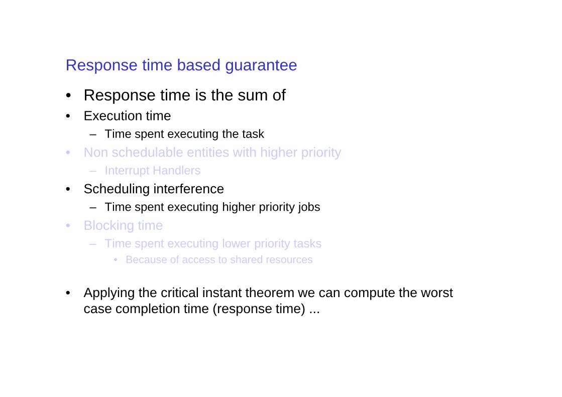
Response time based guarantee
• Response time is the sum of• Execution time
– Time spent executing the task
• Non schedulable entities with higher priority– Interrupt Handlers
• Scheduling interference– Time spent executing higher priority jobs
• Blocking time– Time spent executing lower priority tasks
• Because of access to shared resources
• Applying the critical instant theorem we can compute the worst case completion time (response time) ...
Theorem 1 Recalled
• Theorem 1: A critical instant for any task occurs whenever the task is requested simultaneously with requests of all higher priority tasks
• Can use this to determine whether a given priority assignment will yield a feasible scheduling algorithm
• if requests for all tasks at their critical instants are fulfilled before their respective deadlines, then the scheduling algorithm is feasible
• Applicable to any static priority scheme… not just RM• Applicable to any static priority scheme… not just RM
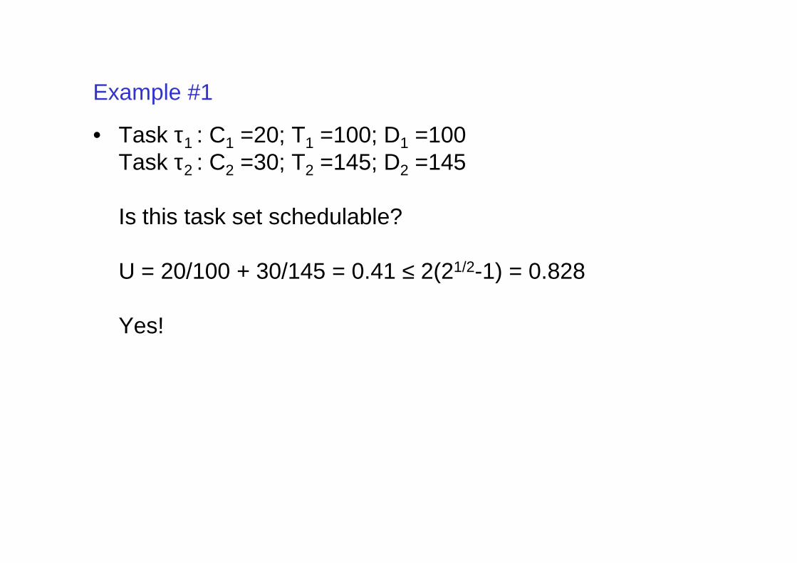
Example #1
• Task τ1 : C1 =20; T1 =100; D1 =100Task τ2 : C2 =30; T2 =145; D2 =145
Is this task set schedulable?
U = 20/100 + 30/145 = 0.41 ≤ 2(21/2-1) = 0.828U = 20/100 + 30/145 = 0.41 ≤ 2(2 -1) = 0.828
Yes!
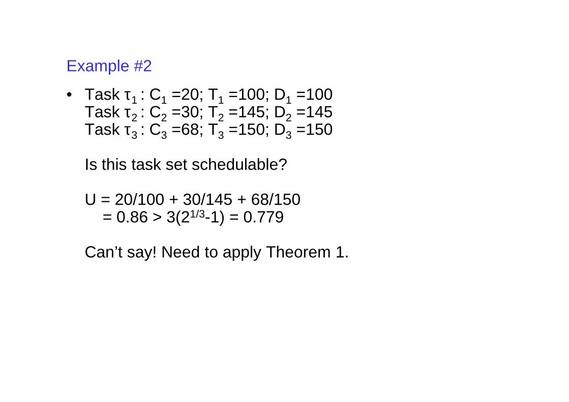
Example #2
• Task τ1 : C1 =20; T1 =100; D1 =100Task τ2 : C2 =30; T2 =145; D2 =145Task τ3 : C3 =68; T3 =150; D3 =150
Is this task set schedulable?
U = 20/100 + 30/145 + 68/150U = 20/100 + 30/145 + 68/150= 0.86 > 3(21/3-1) = 0.779
Can’t say! Need to apply Theorem 1.
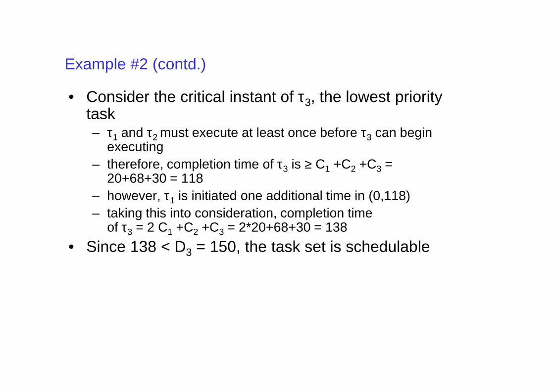
Example #2 (contd.)
• Consider the critical instant of τ3, the lowest priority task– τ1 and τ2 must execute at least once before τ3 can begin
executing– therefore, completion time of τ3 is ≥ C1 +C2 +C3 =
20+68+30 = 118– however, τ1 is initiated one additional time in (0,118)– however, τ1 is initiated one additional time in (0,118)– taking this into consideration, completion time
of τ3 = 2 C1 +C2 +C3 = 2*20+68+30 = 138
• Since 138 < D3 = 150, the task set is schedulable
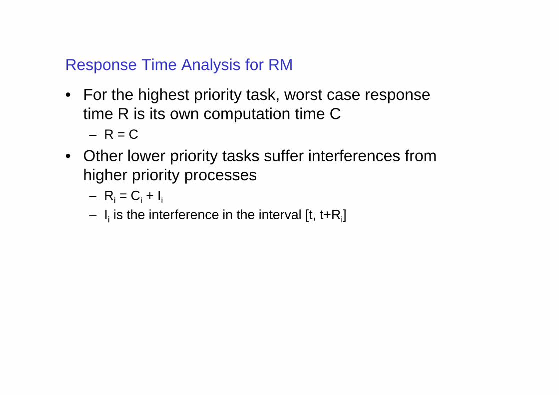
Response Time Analysis for RM
• For the highest priority task, worst case response time R is its own computation time C– R = C
• Other lower priority tasks suffer interferences from higher priority processes– Ri = Ci + Ii– Ri = Ci + Ii– Ii is the interference in the interval [t, t+Ri]
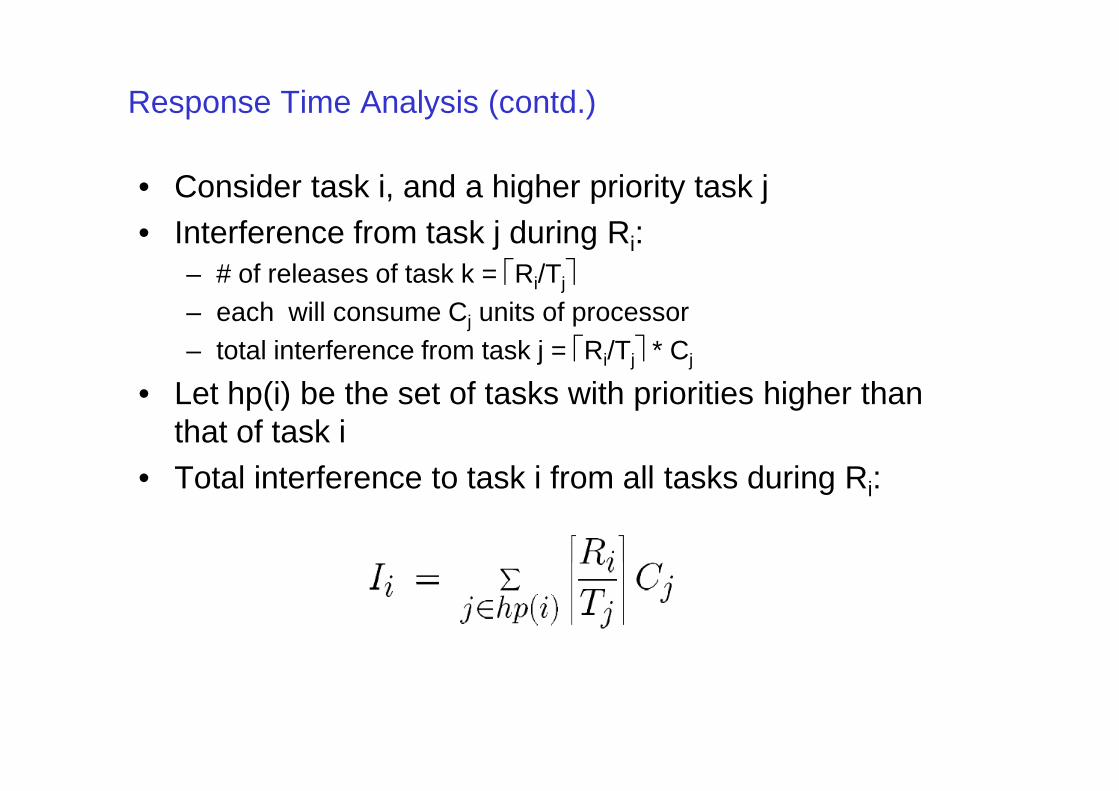
Response Time Analysis (contd.)
• Consider task i, and a higher priority task j• Interference from task j during Ri:
– # of releases of task k = Ri/Tj
– each will consume Cj units of processor– total interference from task j = Ri/Tj * Cj
• Let hp(i) be the set of tasks with priorities higher than • Let hp(i) be the set of tasks with priorities higher than that of task i
• Total interference to task i from all tasks during Ri:
Response Time Analysis (contd.)
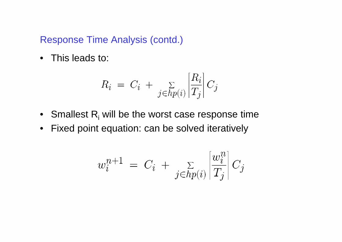
• This leads to:
• Smallest Ri will be the worst case response timei
• Fixed point equation: can be solved iteratively
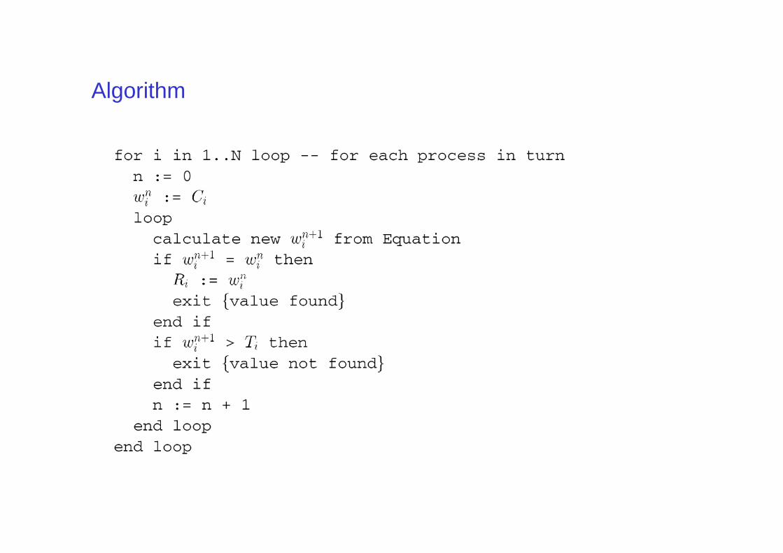
Algorithm
Deadline Monotonic (DM)
• If deadlines are different from the periods, then RM is no more optimal
• If deadlines are lower than periods the Deadline Monotonic policy is optimal among all fixed-priority schemes

Deadline Monotonic (DM)
• Fixed priority of a process is inversely proportional to its deadline (< period)
Di < Dj ⇒ Pi > Pj
• Optimal: can schedule any task set that any other static priority assignment can
• Example: RM fails but DM succeeds for the following• Example: RM fails but DM succeeds for the following
Deadline Monotonic (DM)
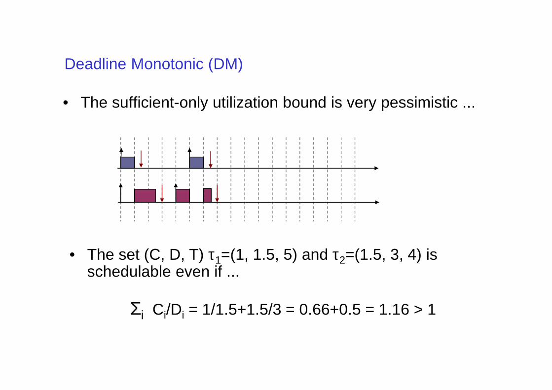
• The sufficient-only utilization bound is very pessimistic ...
• The set (C, D, T) τ1=(1, 1.5, 5) and τ2=(1.5, 3, 4) is schedulable even if ...
Σi Ci/Di = 1/1.5+1.5/3 = 0.66+0.5 = 1.16 > 1
Can one do better?
• Yes… by using dynamic priority assignment
• In fact, there is a scheme for dynamic priority assignment for which the least upper bound on the processor utilization is 1
• More later...
Arbitrary Deadlines
• Case when deadline Di < Ti is easy…• Case when deadline Di > Ti is much harder
– multiple iterations of the same task may be alive simultaneously
– may have to check multiple task initiations to obtain the worst case response time
• Example: consider two tasks• Example: consider two tasks– Task 1: C1 = 28, T1 = 80– Task 2: C2 = 71, T2 = 110– Assume all deadlines to be infinity
Arbitrary Deadlines (contd.)
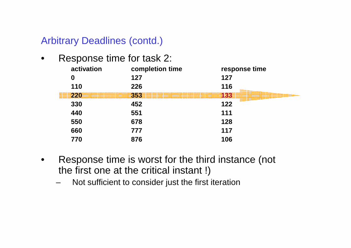
• Response time for task 2:activation completion time response time0 127 127110 226 116220 353 133330 452 122440 551 111550 678 128550 678 128660 777 117770 876 106
• Response time is worst for the third instance (not the first one at the critical instant !)
– Not sufficient to consider just the first iteration
Arbitrary Deadlines (contd.)
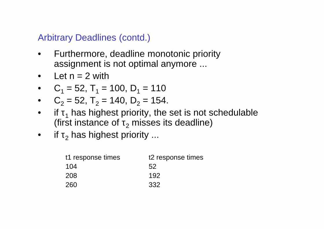
• Furthermore, deadline monotonic priority assignment is not optimal anymore ...
• Let n = 2 with • C1 = 52, T1 = 100, D1 = 110• C2 = 52, T2 = 140, D2 = 154.• if τ1 has highest priority, the set is not schedulable • if τ1 has highest priority, the set is not schedulable
(first instance of τ2 misses its deadline)• if τ2 has highest priority ...
t1 response times t2 response times104 52208 192260 332
Arbitrary Deadlines (contd.)
• Can we find a schedulability test ?– Yes
• Can we find an optimal priority assignment ?– Yes
Schedulability Condition for Arbitrary Deadlines
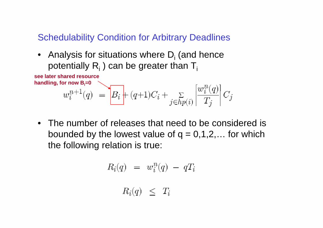
• Analysis for situations where Di (and hence potentially Ri ) can be greater than Ti
see later shared resource handling, for now Bi=0
• The number of releases that need to be considered is bounded by the lowest value of q = 0,1,2,… for which the following relation is true:
Arbitrary Deadlines (contd.)
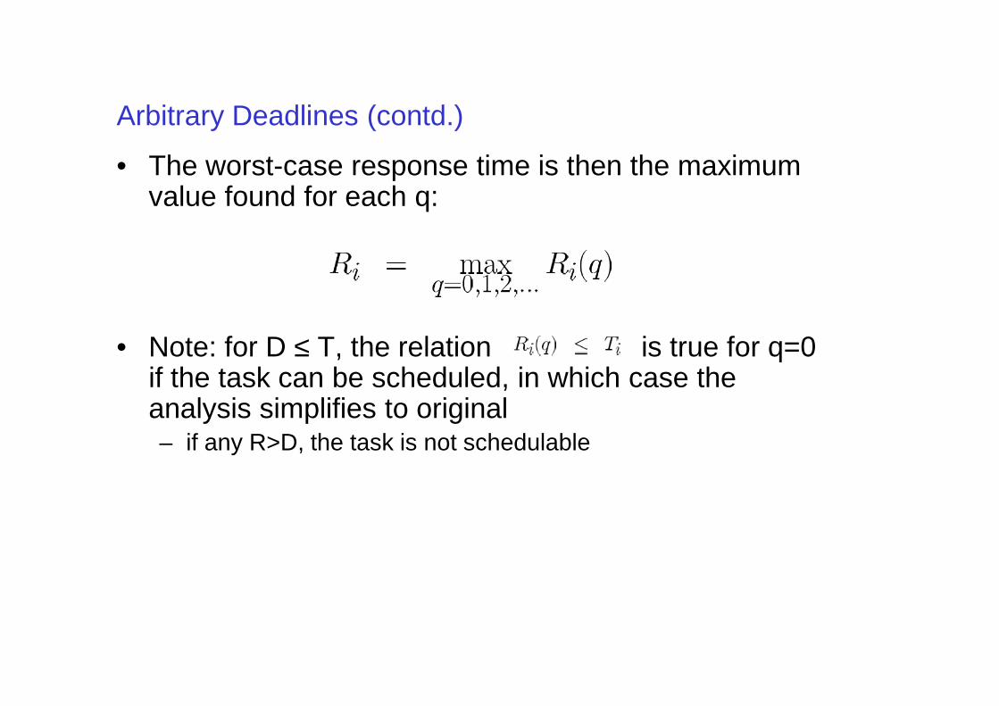
• The worst-case response time is then the maximum value found for each q:
• Note: for D ≤ T, the relation is true for q=0 • Note: for D ≤ T, the relation is true for q=0 if the task can be scheduled, in which case the analysis simplifies to original– if any R>D, the task is not schedulable
Optimal priority assignment for Arbitrary Deadlines
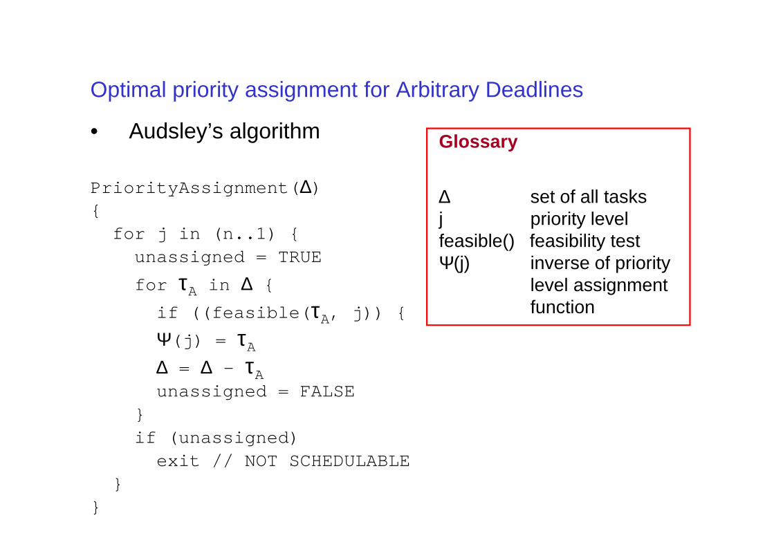
• Audsley’s algorithm
PriorityAssignment( ∆){
for j in (n..1) {unassigned = TRUE
τ ∆
Glossary
∆ set of all tasksj priority levelfeasible() feasibility testΨ(j) inverse of priority
for τA in ∆ {
if ((feasible( τA, j)) {
Ψ(j) = τA
∆ = ∆ – τAunassigned = FALSE
}if (unassigned)
exit // NOT SCHEDULABLE}
}
level assignment function
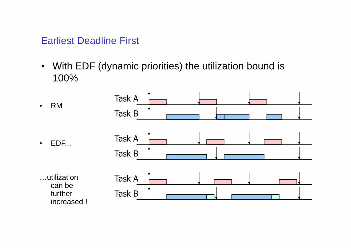
• With EDF (dynamic priorities) the utilization bound is 100%
Earliest Deadline First
Task A
Task B• RM
…utilization can be further increased !
Task A
Task B
Task A
Task B
• EDF...
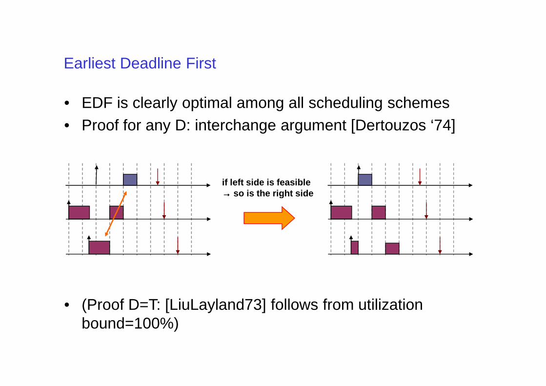
• EDF is clearly optimal among all scheduling schemes• Proof for any D: interchange argument [Dertouzos ‘74]
Earliest Deadline First
if left side is feasible →→→→ so is the right side
• (Proof D=T: [LiuLayland73] follows from utilization bound=100%)
→→→→ so is the right side
Earliest Deadline First
• There are few (if any) commercial implementations of EDF
“EDF implementations are inefficient and should be avoided because a RT system should be as fast as possible”
“EDF cannot be controlled in overload conditions”
Implementation of Earliest Deadline First
• Is it really not feasible to implement EDF scheduling ?
• Problems– absolute deadlines change for each new task instance,
therefore the priority needs to be updated every time the task moves back to the ready queuemoves back to the ready queue
– more important, absolute deadlines are always increasing, how can we associate a (finite) priority value to an ever-increasing deadline value
– most important, absolute deadlines are impossible to compute a-priori (there are infinitely many). Do we need infinitely many priority levels?
– What happens in overload conditions?
Implementation of fixed priority
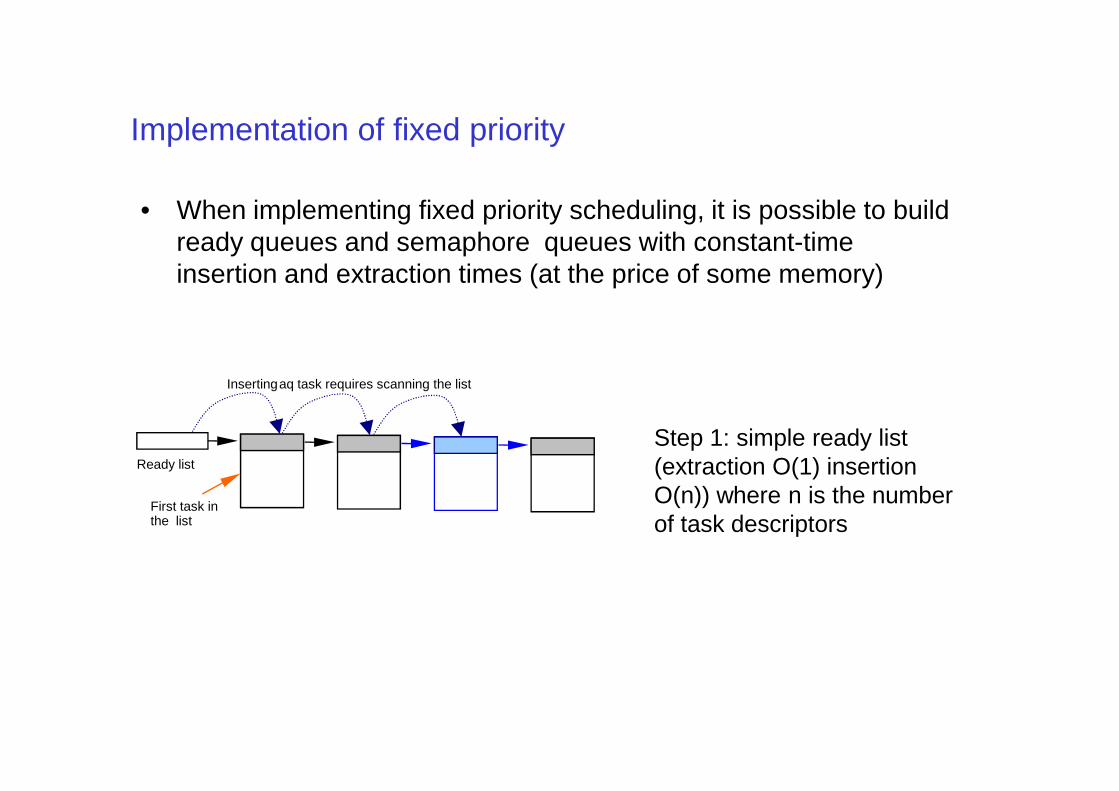
• When implementing fixed priority scheduling, it is possible to build ready queues and semaphore queues with constant-time insertion and extraction times (at the price of some memory)
Inserting aq task requires scanning the list
Ready list
First task inthe list
Step 1: simple ready list (extraction O(1) insertion O(n)) where n is the number of task descriptors
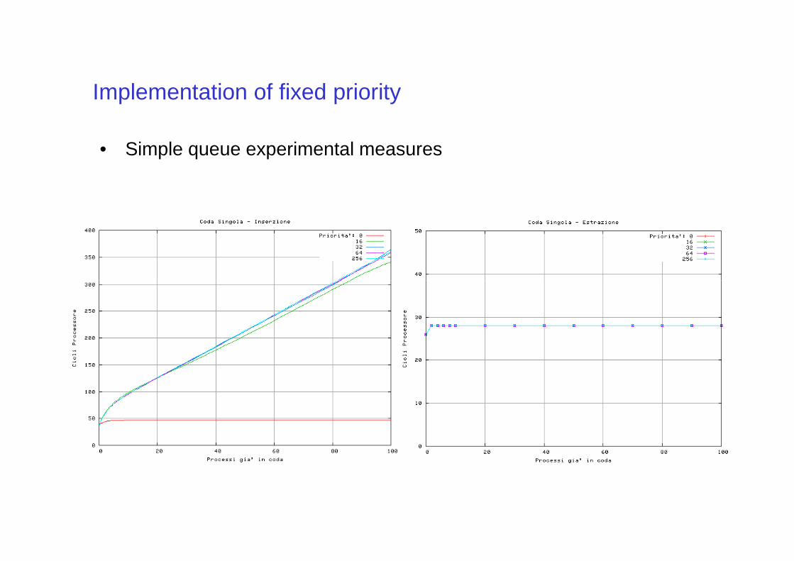
Implementation of fixed priority
• Simple queue experimental measures
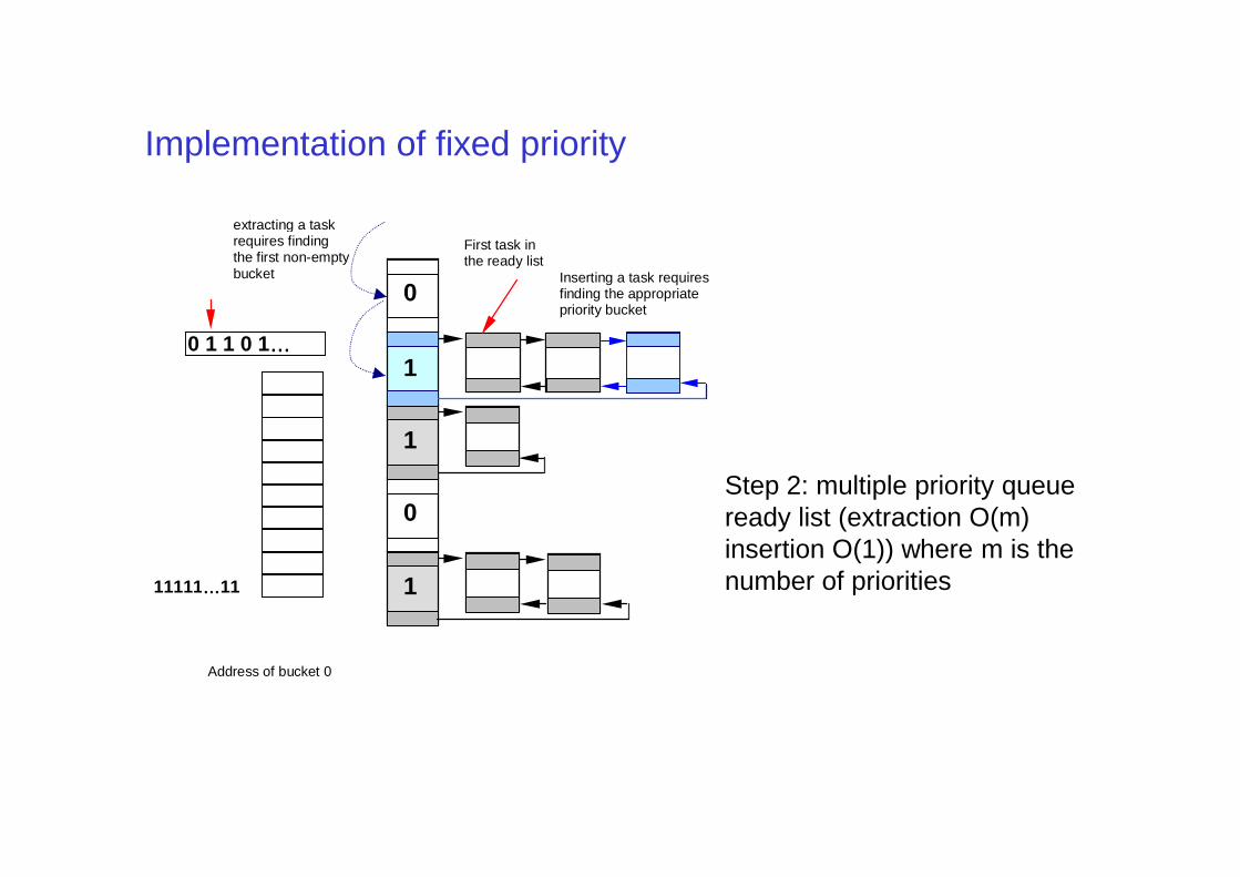
Implementation of fixed priority
First task inthe ready list
extracting a taskrequires findingthe first non-emptybucket Inserting a task requires
finding the appropriatepriority bucket
0
1
1
0 1 1 0 1…………
Step 2: multiple priority queue ready list (extraction O(m) insertion O(1)) where m is the number of priorities
0
1
111111…………11
Address of bucket 0
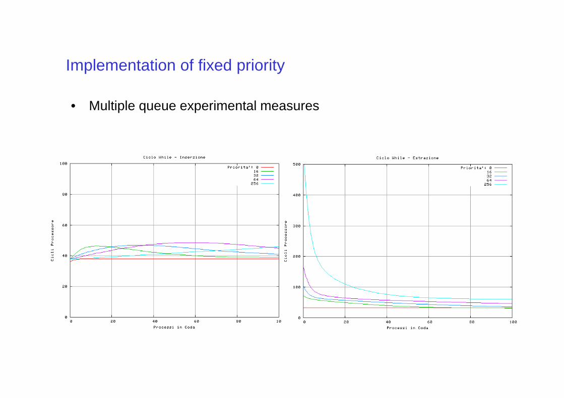
Implementation of fixed priority
• Multiple queue experimental measures
Implementation of fixed priority
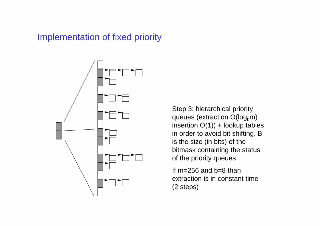
Step 3: hierarchical priority queues (extraction O(logbm) insertion O(1)) + lookup tables in order to avoid bit shifting. B is the size (in bits) of the bitmask containing the status of the priority queues
If m=256 and b=8 than extraction is in constant time (2 steps)
Implementation of fixed priority
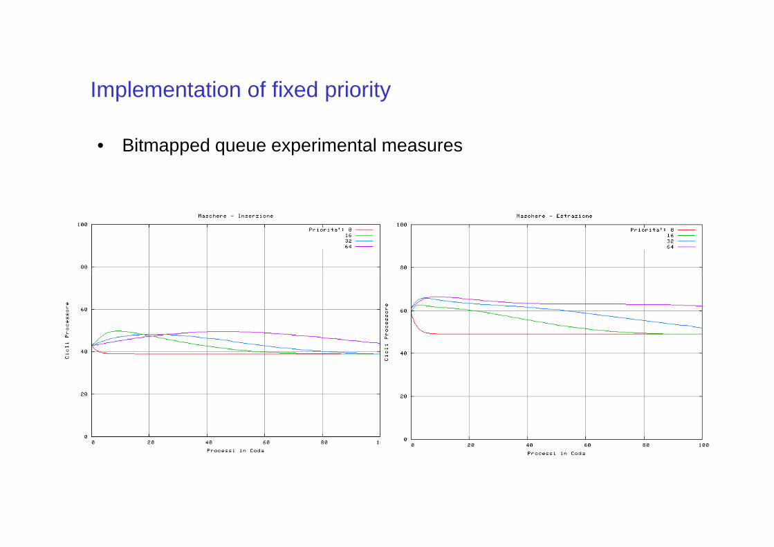
• Bitmapped queue experimental measures
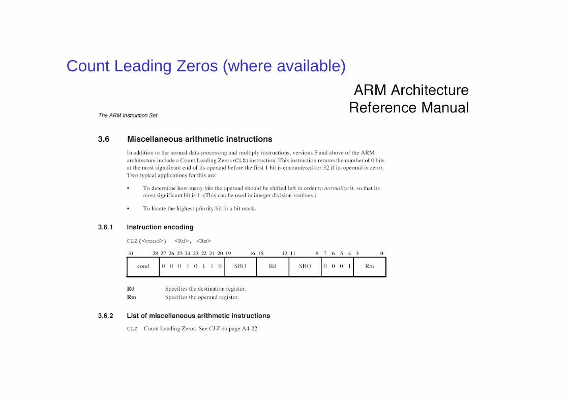
Count Leading Zeros (where available)
Implementation of fixed priority
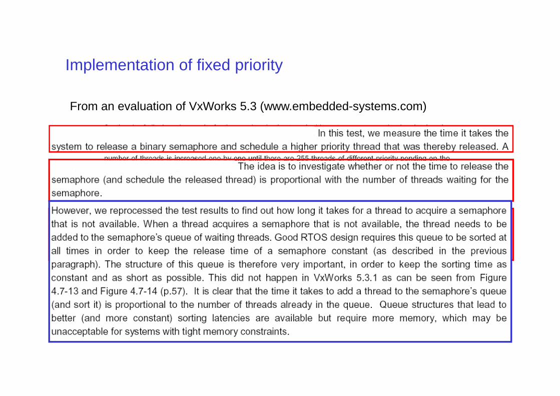
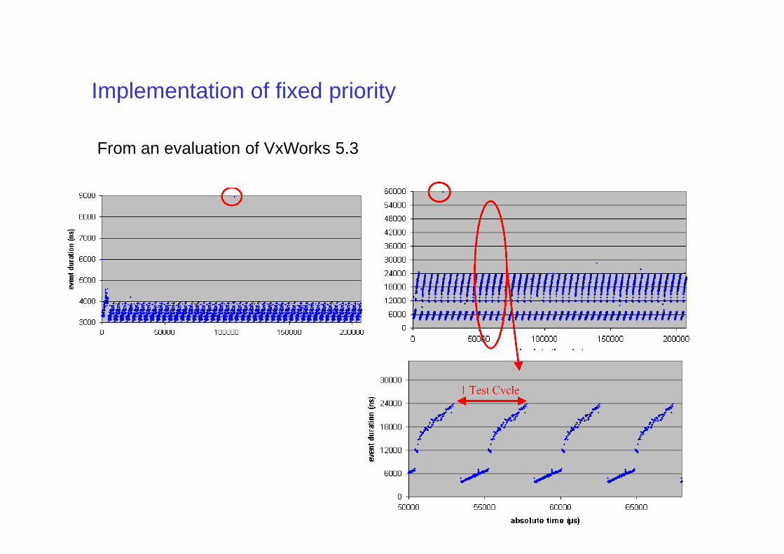
From an evaluation of VxWorks 5.3 (www.embedded-systems.com)
Implementation of fixed priority
From an evaluation of VxWorks 5.3
Implementation of Earliest Deadline First
• Problem 2: deadline encoding ?– The EDF scheduler, requires a time reference to compute the
absolute deadline (the priority) of a newly activated task. Sucha timer must necessarily feature a long lifetime and a shortgranularity. For example, in POSIX systems, a 64 bit structureallows for a granularity of nanoseconds. In an embeddedallows for a granularity of nanoseconds. In an embeddedsystem, such a high precision might actually becomeundesirable since it leads to an unacceptable overhead.
Implementation of Earliest Deadline First
• Problem 2: deadline encoding ?– The problem can be efficiently solved using a limited resolution
(i.e. 16 bit) timer and an algorithm first described in[Fonseca01]. Suppose the current timer value and theabsolute deadlines are represented as 16 bit words. Each timea task is activated, the system computes an absolute deadlinea task is activated, the system computes an absolute deadlinefor it as the current timer value plus the task's relativedeadline: this operation could result in an overflow. However,ignoring overflows, it is still possible to compare two absolutedeadlines in a consistent way. Suppose that the maximumrelative deadline is less than 7FFFh timer ticks, and let δ bethe difference between two absolute deadlines d1 and d2: δ isalways in the interval [-8000h; +7FFFh] and can beexpressed as a signed 16 bit integer. The sign of δ can beused as a way to compare d1 and d2: if δ >0 then d1>d2.
Implementation of Earliest Deadline First
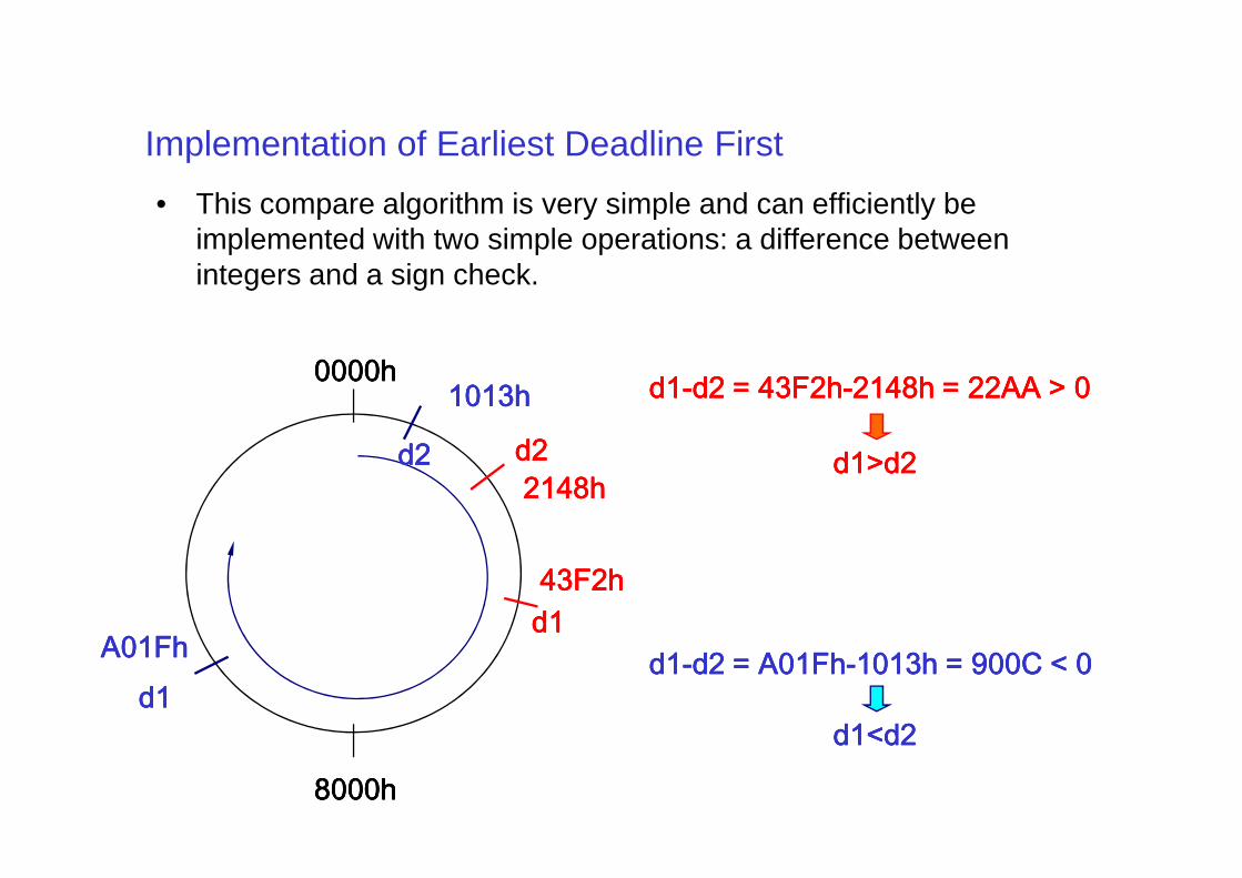
• This compare algorithm is very simple and can efficiently be implemented with two simple operations: a difference between integers and a sign check.
0000h0000h0000h0000h
d2d2d2d2
d1d1d1d1----d2 = 43F2hd2 = 43F2hd2 = 43F2hd2 = 43F2h----2148h = 22AA > 02148h = 22AA > 02148h = 22AA > 02148h = 22AA > 0
d2d2d2d2
1013h1013h1013h1013h
8000h8000h8000h8000h
43F2h43F2h43F2h43F2hd1d1d1d1
d2d2d2d22148h2148h2148h2148h
d1>d2d1>d2d1>d2d1>d2
A01FhA01FhA01FhA01Fhd1d1d1d1
d2d2d2d2
d1d1d1d1----d2 = A01Fhd2 = A01Fhd2 = A01Fhd2 = A01Fh----1013h = 900C < 01013h = 900C < 01013h = 900C < 01013h = 900C < 0
d1<d2d1<d2d1<d2d1<d2
Implementation of Earliest Deadline First
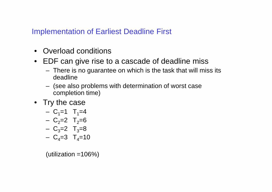
• Overload conditions• EDF can give rise to a cascade of deadline miss
– There is no guarantee on which is the task that will miss its deadline
– (see also problems with determination of worst case completion time)completion time)
• Try the case– C1=1 T1=4– C2=2 T2=6– C3=2 T3=8– C4=3 T4=10
(utilization =106%)
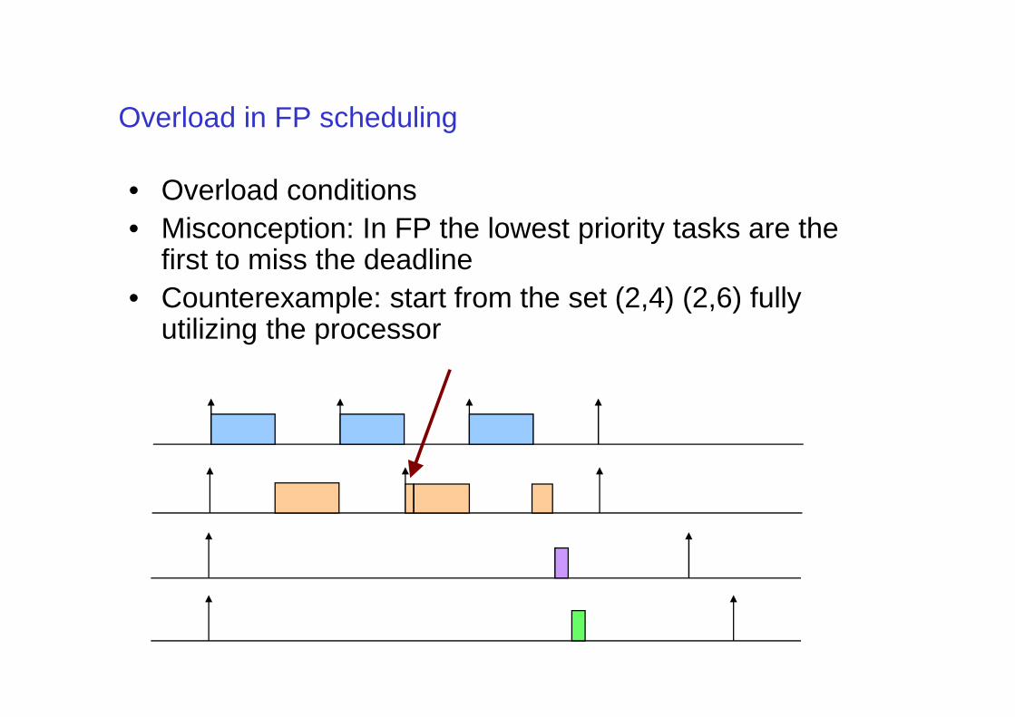
Overload in FP scheduling
• Overload conditions• Misconception: In FP the lowest priority tasks are the
first to miss the deadline• Counterexample: start from the set (2,4) (2,6) fully
utilizing the processor
Task Synchronization
• So far, we considered independent tasks• However, tasks do interact: semaphores, locks,
monitors, rendezvous etc.• shared data, use of non-preemptable resources
• This jeopardizes systems ability to meet timing constraintsconstraints
• e.g. may lead to an indefinite period of priority inversion where a high priority task is prevented from executing by a low priority task
Optimality and Ulub
• When there are shared resources ...– The RM priority assignment is no more optimal. As a matter
of fact, there is no optimal priority assignment (NP-complete problem [Mok])
– The least upper bound on processor utilization can be arbitrarily low
• It is possible (and quite easy as a matter of fact) to build a sample task set which is not schedulable in spite of a utilization sample task set which is not schedulable in spite of a utilization U → 0
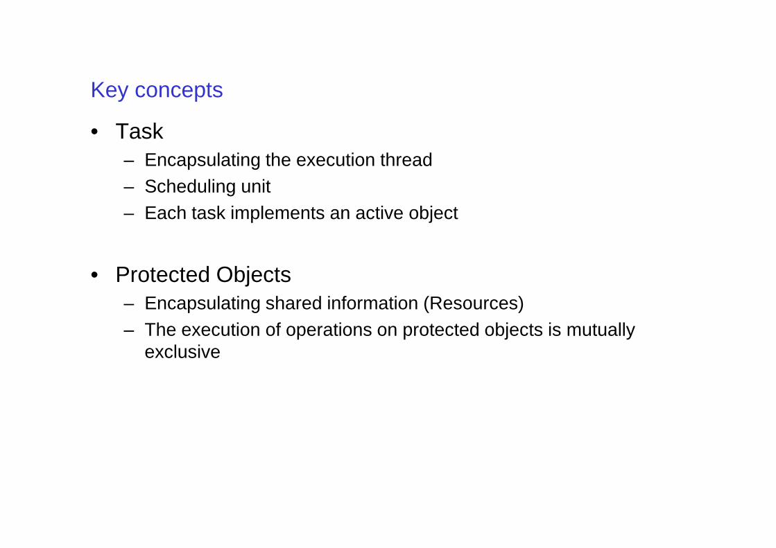
Key concepts
• Task– Encapsulating the execution thread – Scheduling unit– Each task implements an active object
• Protected Objects• Protected Objects– Encapsulating shared information (Resources)– The execution of operations on protected objects is mutually
exclusive
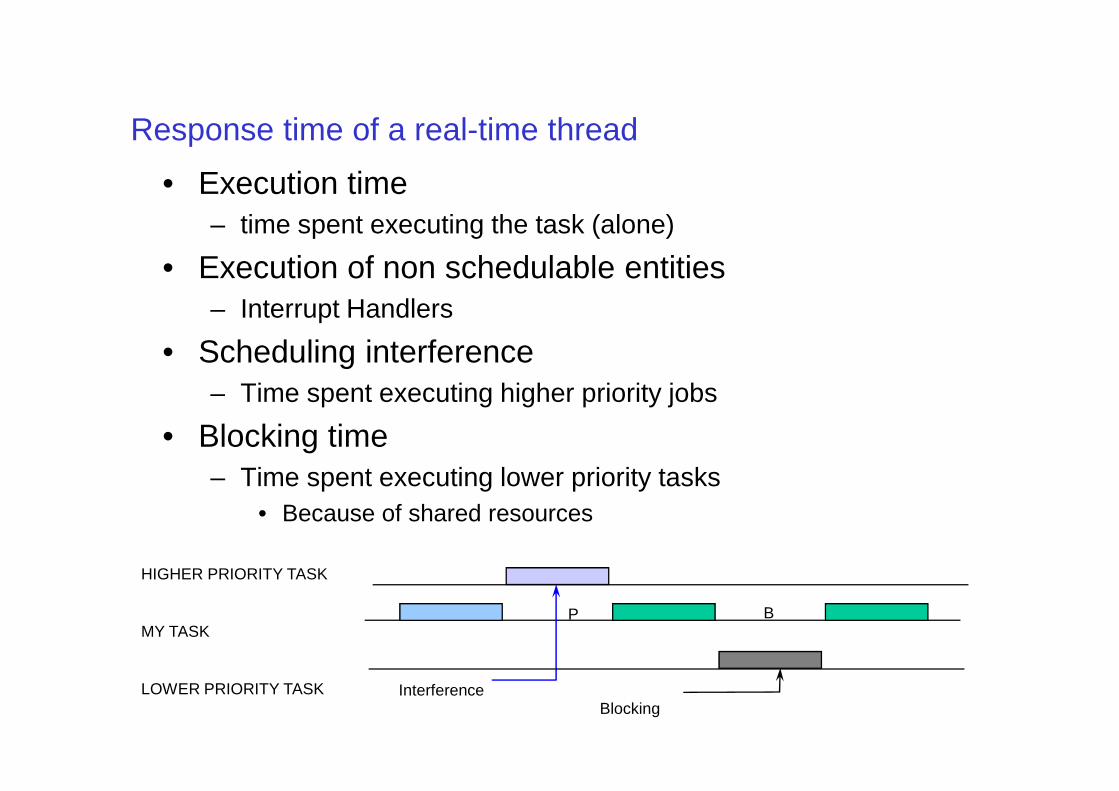
Response time of a real-time thread
• Execution time– time spent executing the task (alone)
• Execution of non schedulable entities – Interrupt Handlers
• Scheduling interference– Time spent executing higher priority jobs– Time spent executing higher priority jobs
• Blocking time– Time spent executing lower priority tasks
• Because of shared resources
HIGHER PRIORITY TASK
MY TASK
LOWER PRIORITY TASK
P B
InterferenceBlocking
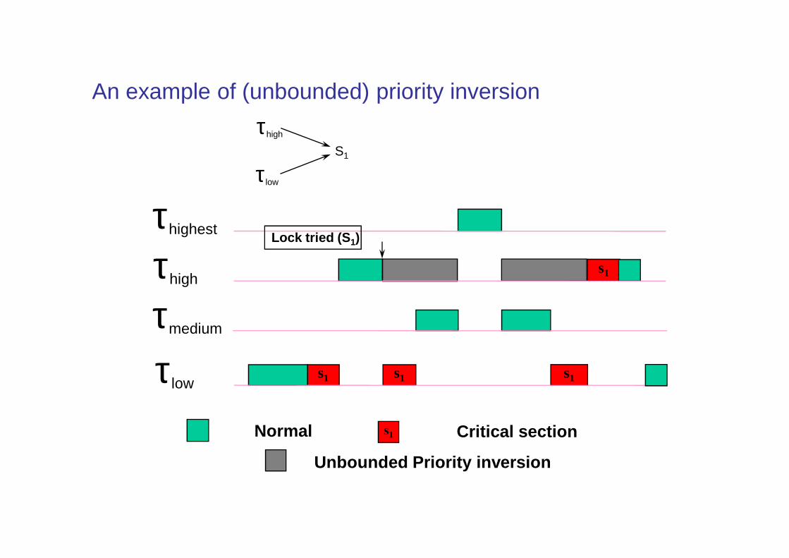
An example of (unbounded) priority inversion
s1
τhigh
τlow
S1
τhigh
τhighestLock tried (S1)
s1 s1 s1
s1Normal Critical section
Unbounded Priority inversion
τhigh
τmedium
τlow
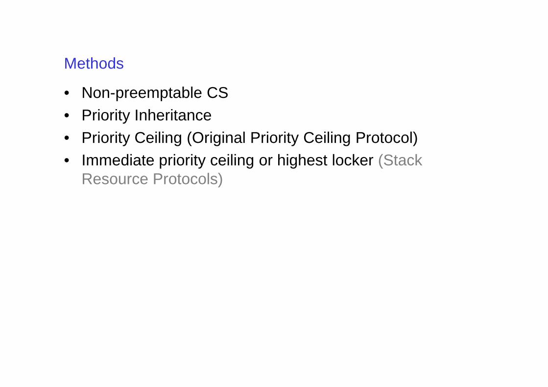
Methods
• Non-preemptable CS• Priority Inheritance• Priority Ceiling (Original Priority Ceiling Protocol)• Immediate priority ceiling or highest locker (Stack
Resource Protocols)
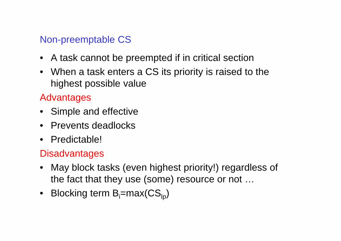
Non-preemptable CS
• A task cannot be preempted if in critical section • When a task enters a CS its priority is raised to the
highest possible valueAdvantages• Simple and effective• Prevents deadlocks• Prevents deadlocks• Predictable!Disadvantages• May block tasks (even highest priority!) regardless of
the fact that they use (some) resource or not …• Blocking term Bi=max(CSlp)
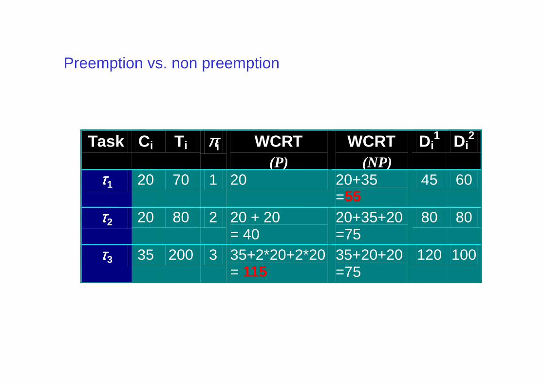
Preemption vs. non preemption
Task Ci Ti ππππi WCRT(P)
Di2
ττττ1 20 70 1 20 60
WCRT(NP)
20+35=55
Di1
45
ττττ2 20 80 2 20 + 20 = 40
80
ττττ3 35 200 3 35+2*20+2*20 = 115
100
=5520+35+20=7535+20+20=75
80
120
Priority Inheritance Protocol
• [Sha89]• Tasks are only blocked when using CS• Avoids unbounded blocking from medium priority
tasks• It is possible to bound the worst case blocking time if
requests are not nestedrequests are not nested• Saved the Mars Pathfinder …
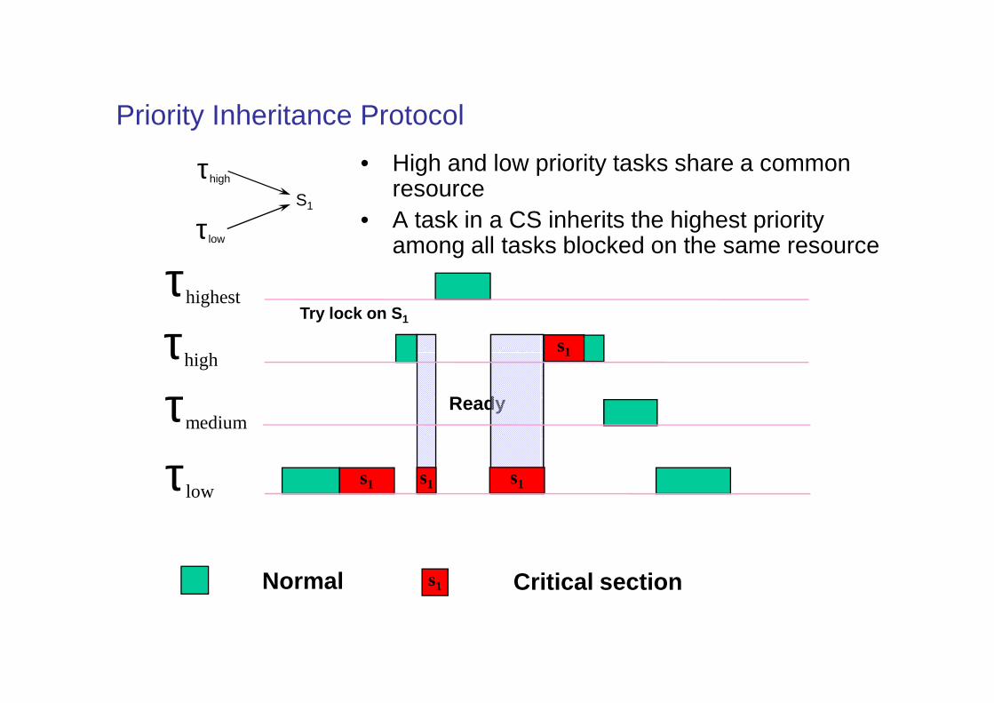
Priority Inheritance Protocol
• High and low priority tasks share a common resource
• A task in a CS inherits the highest priority among all tasks blocked on the same resource
s1
τhigh
τlow
S1
Try lock on S1
τhigh
τhighest
s1
s1Normal Critical section
s1 s1
Ready
s1
τhigh
τmedium
τlow
priority inheritance
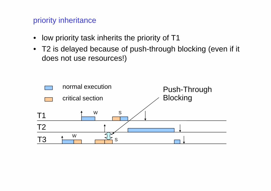
• low priority task inherits the priority of T1• T2 is delayed because of push-through blocking (even if it
does not use resources!)
critical section
normal execution Push-ThroughBlocking
T1
T2
T3
critical section
SW
W S
Blocking
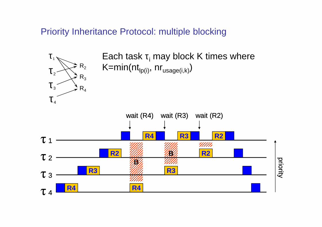
Priority Inheritance Protocol: multiple blocking
τ1
R2
R3
τ2
τ3
wait (R4)wait (R4) wait (R3)wait (R3) wait (R2)wait (R2)
τ4
R4
Each task τi may block K times where K=min(ntlp(i), nrusage(i,k))
BB
prioritypriority
R4
R3
R2
wait (R4)wait (R4)
R4ττ 44
ττ 33
ττ 22
ττ 11R4
wait (R3)wait (R3)
R3
R3
wait (R2)wait (R2)
R2
R2
Priority Inheritance Protocol
• Disadvantages• Tasks may block multiple times• Worst case behavior even worse than non-
preemptable CS• Costly implementation except for very simple cases• Does not even prevent deadlock• Does not even prevent deadlock
Priority Ceiling Protocol
• priority ceiling of a resource S = maximum priority among all tasks that can possibly access S
• A process can only lock a resource if its dynamic priority is higher than the ceiling of any currently locked resource (excluding any that it has already locked itself).
• If task τ blocks, the task holding the lock on the blocking resource inherits its priorityinherits its priority
• Two forms– Original ceiling priority protocol (OCPP)– Immediate ceiling priority protocol (ICPP, similar to Stack Resource
Policy SRP)
• Properties (on single processor systems)– A high priority process can be blocked at most once during its execution
by lower priority processes– Deadlocks are prevented– Transitive blocking is prevented

Example of OCPP
wait (R4)wait (R4) wait (R3)wait (R3) wait (R2)wait (R2)
τ1
R2
R3
τ2
τ3
τ4
R4 ceiling R4 = 1
ceiling R3 = 1
ceiling R2 = 1
B
prioritypriority
R4
R3
R2
R4ττ 44
ττ 33
ττ 22
ττ 11R4 R3 R2
wait (R3)wait (R3)
wait (R2)wait (R2)
Immediate Priority Ceiling Protocol
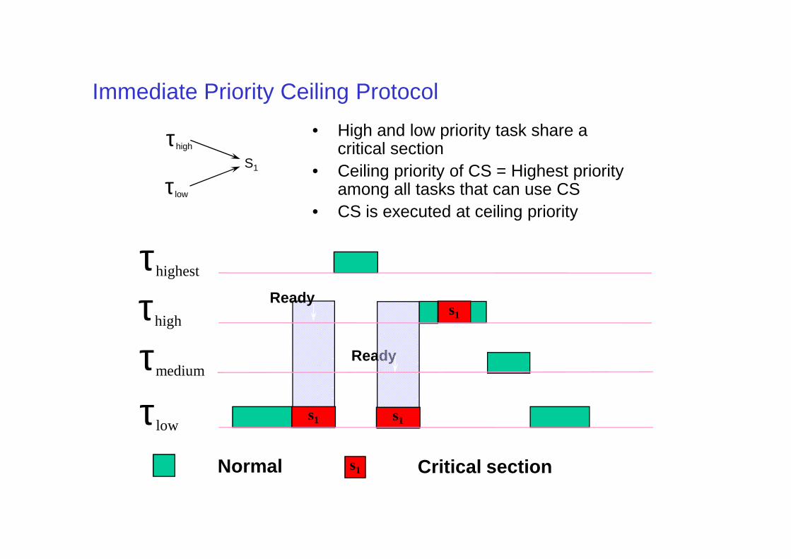
• High and low priority task share a critical section
• Ceiling priority of CS = Highest priority among all tasks that can use CS
• CS is executed at ceiling priority
τhigh
τlow
S1
τhighest
s1Normal Critical section
s1
s1
Ready
Ready
s1
τhigh
τmedium
τlow
Example of ICPP
τ1
R2
R3
τ2
τ3
τ4
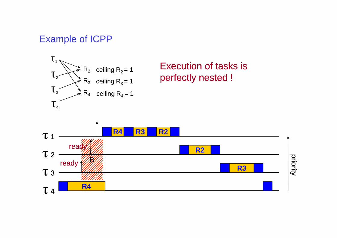
R4 ceiling R4 = 1
ceiling R3 = 1
ceiling R2 = 1 Execution of tasks is Execution of tasks is perfectly nested !perfectly nested !
B
prioritypriority
R4
R3
R2
ττ 44
ττ 33
ττ 22
ττ 11R4 R3 R2
readyready
readyready
OCPP vs. ICPP
• Worst case behavior identical from a scheduling point of view• ICCP is easier to implement than the original (OCPP) as
blocking relationships need not be monitored• ICPP leads to less context switches as blocking is prior to first
execution• ICPP requires more priority movements as this happens with all
resource usages; OCPP only changes priority if an actual block resource usages; OCPP only changes priority if an actual block has occurred.
Response time analysis
Computation
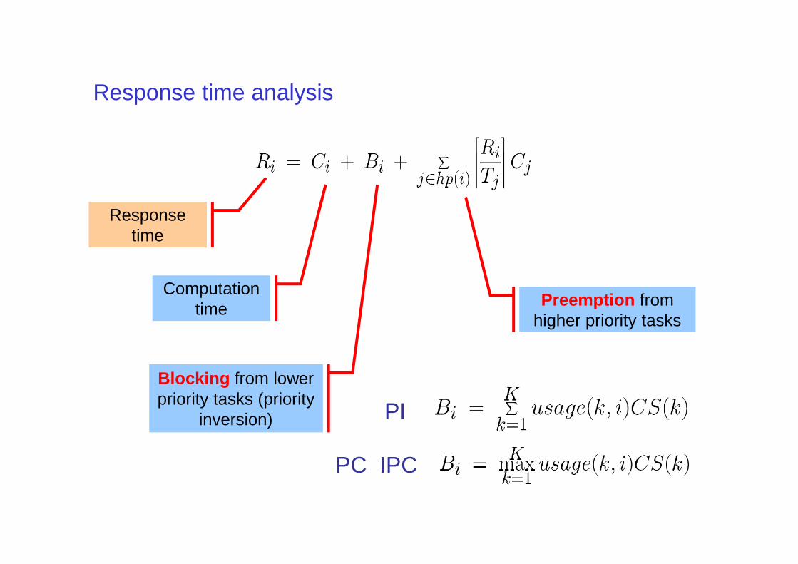
Response time
Computation time
Blocking from lower priority tasks (priority
inversion)
Preemption from higher priority tasks
PI
PC IPC
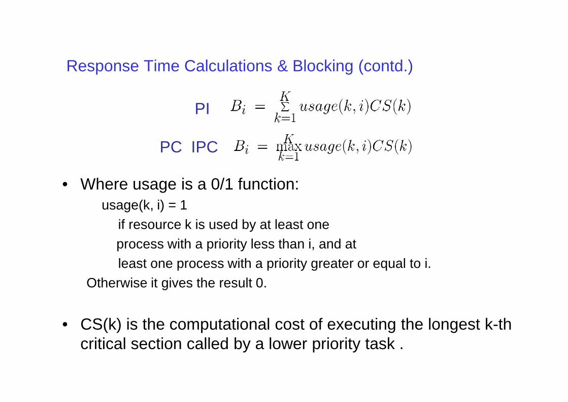
Response Time Calculations & Blocking (contd.)
• Where usage is a 0/1 function:usage(k, i) = 1
PI
PC IPC
usage(k, i) = 1if resource k is used by at least oneprocess with a priority less than i, and atleast one process with a priority greater or equal to i.
Otherwise it gives the result 0.
• CS(k) is the computational cost of executing the longest k-th critical section called by a lower priority task .
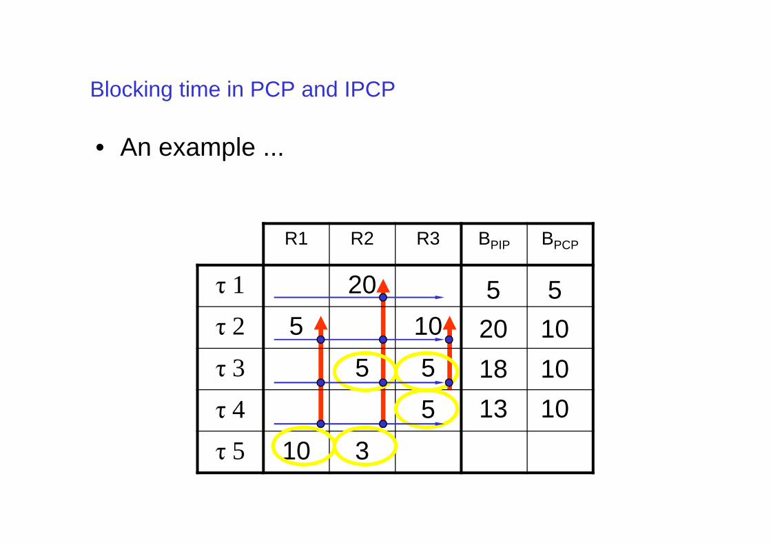
Blocking time in PCP and IPCP
• An example ...
R1 R2 R3 BPIP BPCP
τ 1 20τ 1 20
τ 2 5 10
τ 3 5 5
τ 4 5
τ 5 10 3
20
5
18
13
5
10
10
10
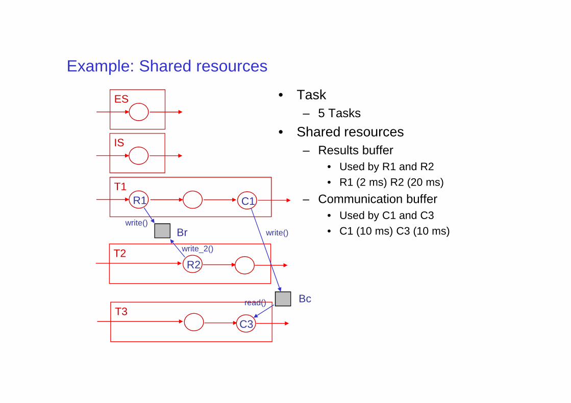
Example: Shared resources
• Task– 5 Tasks
• Shared resources– Results buffer
• Used by R1 and R2• R1 (2 ms) R2 (20 ms)
– Communication buffer
ES
IS
T1R1 C1 – Communication buffer
• Used by C1 and C3• C1 (10 ms) C3 (10 ms)Br
R1 C1
T2
Bc
R2
write()
write_2()
T3C3
write()
read()
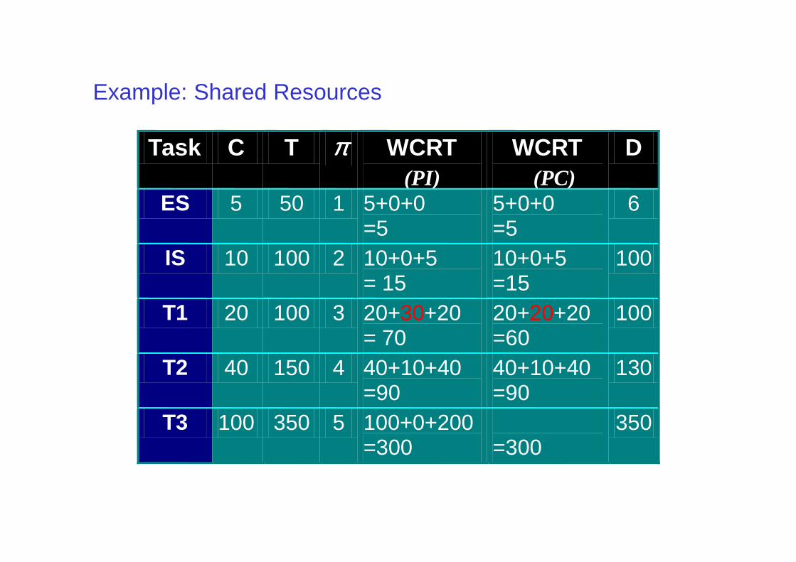
Example: Shared Resources
Task C T ππππ D
ES 5 50 1 6
IS 10 100 2 100
WCRT(PI)
WCRT(PC)
5+0+0=5
5+0+0=5
10+0+5 = 15
10+0+5=15
T1 20 100 3 100
T2 40 150 4 130
T3 100 350 5 100+0+200 350
= 15 =1520+30+20= 70
20+20+20=60
40+10+40=90
40+10+40=90
100+0+200=300 =300
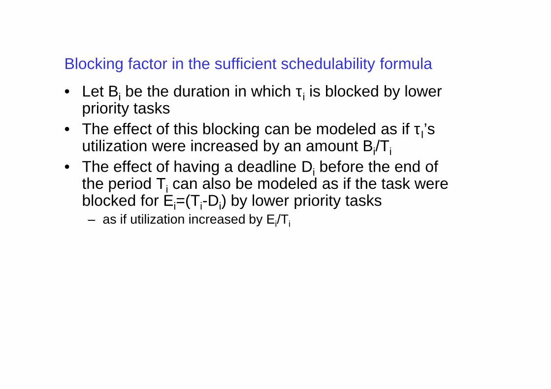
Blocking factor in the sufficient schedulability formula
• Let Bi be the duration in which τi is blocked by lower priority tasks
• The effect of this blocking can be modeled as if τI’s utilization were increased by an amount Bi/Ti
• The effect of having a deadline Di before the end of the period Ti can also be modeled as if the task were blocked for E =(T -D ) by lower priority tasks
iblocked for Ei=(Ti-Di) by lower priority tasks– as if utilization increased by Ei/Ti
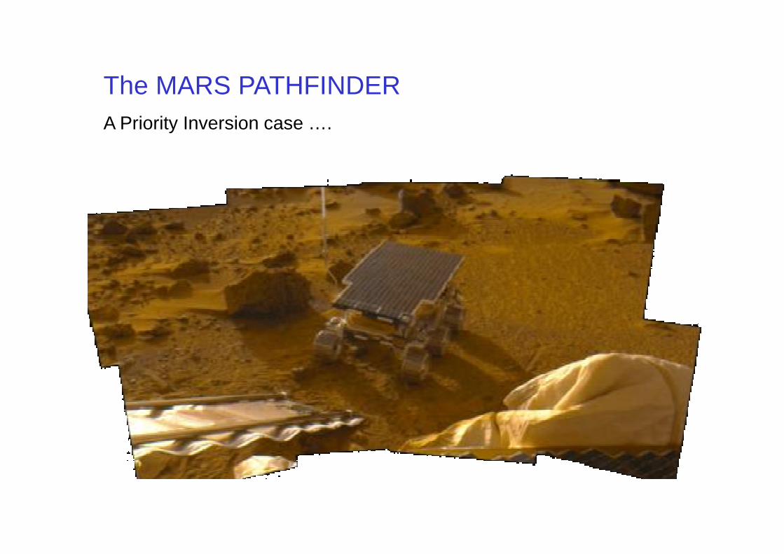
The MARS PATHFINDERA Priority Inversion case ….
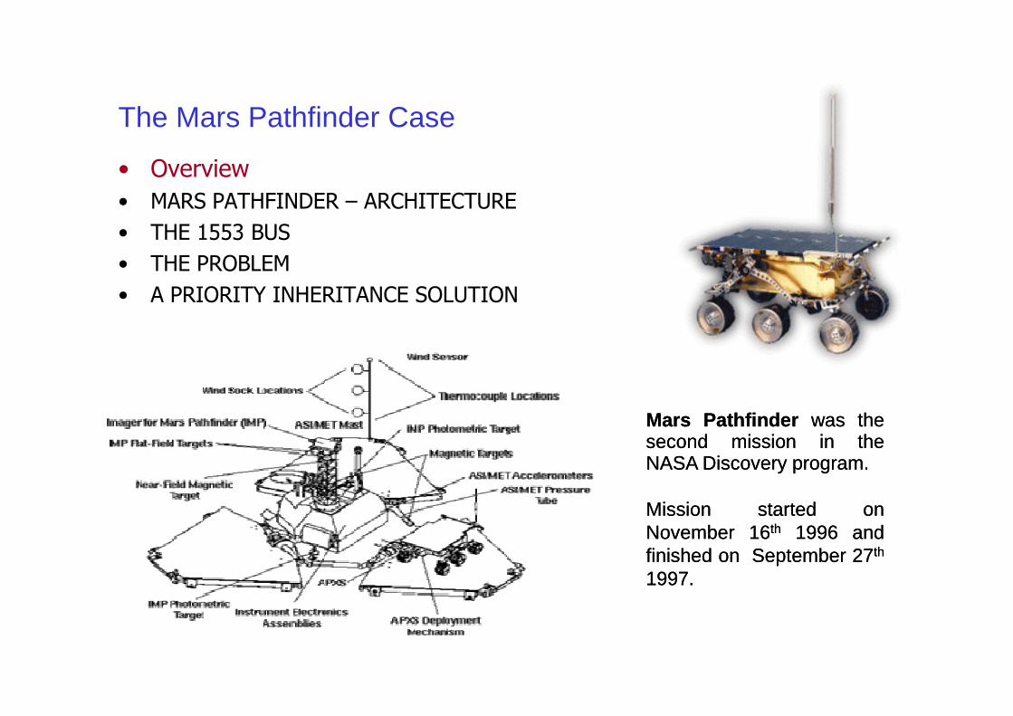
The Mars Pathfinder Case
• Overview
• MARS PATHFINDER – ARCHITECTURE
• THE 1553 BUS
• THE PROBLEM
• A PRIORITY INHERITANCE SOLUTION
MarsMars PathfinderPathfinder waswas thethesecondsecond missionmission inin thetheNASANASA DiscoveryDiscovery programprogram..
MissionMission startedstarted ononNovemberNovember 1616thth 19961996 andandfinishedfinished onon SeptemberSeptember 2727thth
19971997..
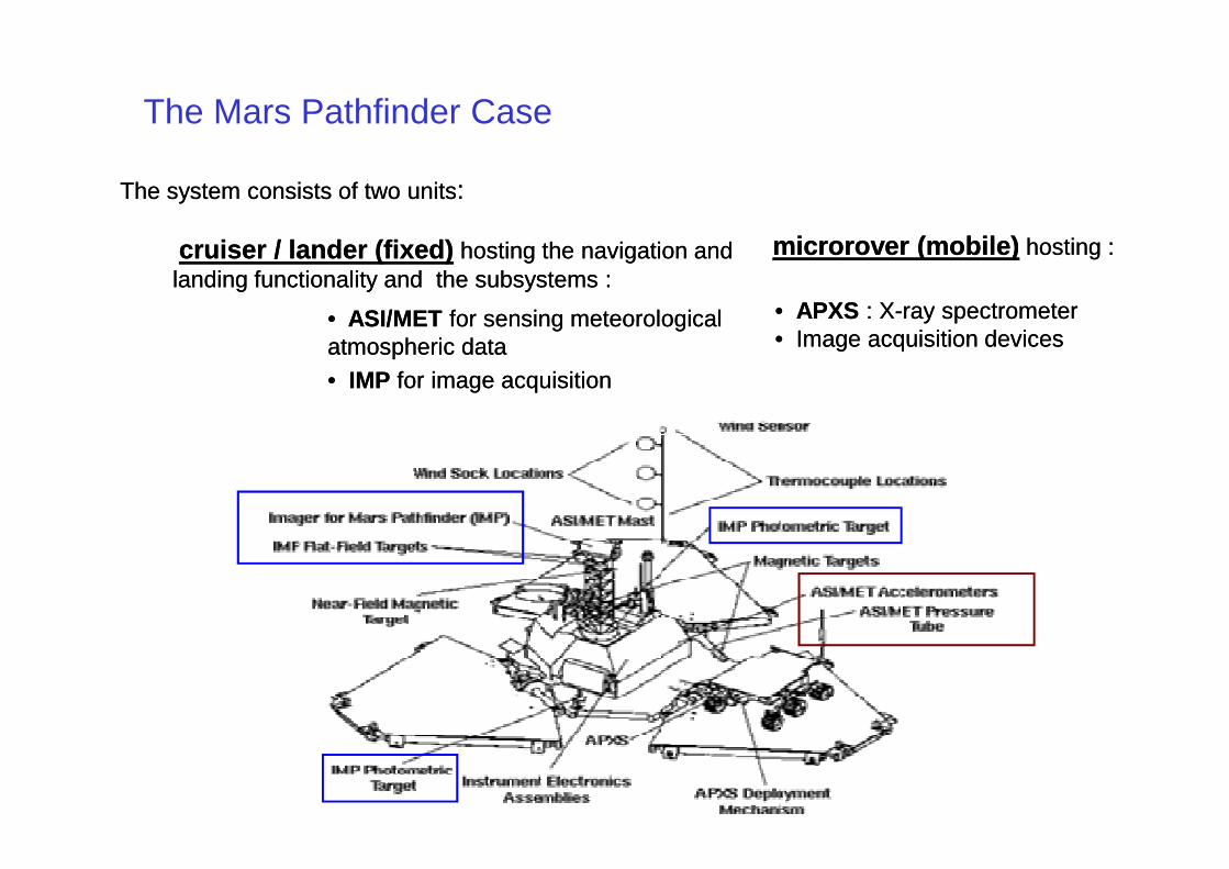
The Mars Pathfinder Case
The system consists of two unitsThe system consists of two units::
cruiser / lander (fixed)cruiser / lander (fixed) hosting the navigation and hosting the navigation and landing functionality and the subsystems :landing functionality and the subsystems :
microrover (mobile)microrover (mobile) hosting :hosting :
•• ASI/METASI/MET for sensing meteorological for sensing meteorological atmospheric dataatmospheric data•• IMPIMP for image acquisitionfor image acquisition
•• APXSAPXS : X: X--ray spectrometerray spectrometer•• Image acquisition devicesImage acquisition devices
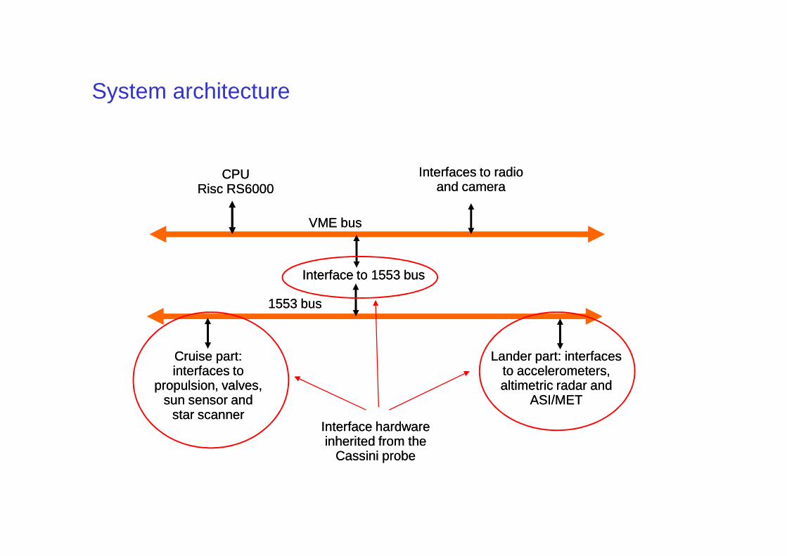
System architecture
CPUCPURisc RS6000Risc RS6000
Interfaces to radio Interfaces to radio and cameraand camera
VME busVME bus
Interface to 1553 busInterface to 1553 busInterface to 1553 busInterface to 1553 bus
1553 bus1553 bus
Cruise part: Cruise part: interfaces to interfaces to
propulsion, valves, propulsion, valves, sun sensor and sun sensor and
star scannerstar scanner
Lander part: interfaces Lander part: interfaces to accelerometers, to accelerometers, altimetric radar and altimetric radar and
ASI/METASI/MET
Interface hardware Interface hardware inherited from the inherited from the
Cassini probeCassini probe
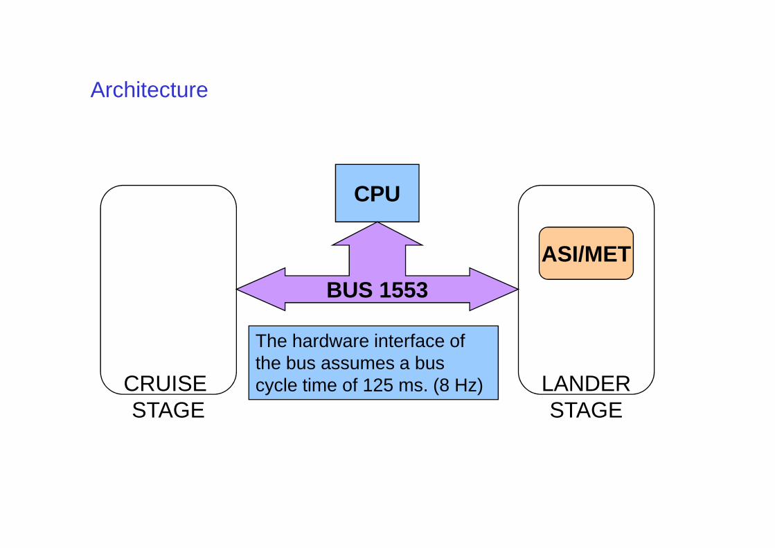
Architecture
CPU
ASI/MET
BUS 1553
CRUISE STAGE
LANDERSTAGE
The hardware interface of the bus assumes a bus cycle time of 125 ms. (8 Hz)
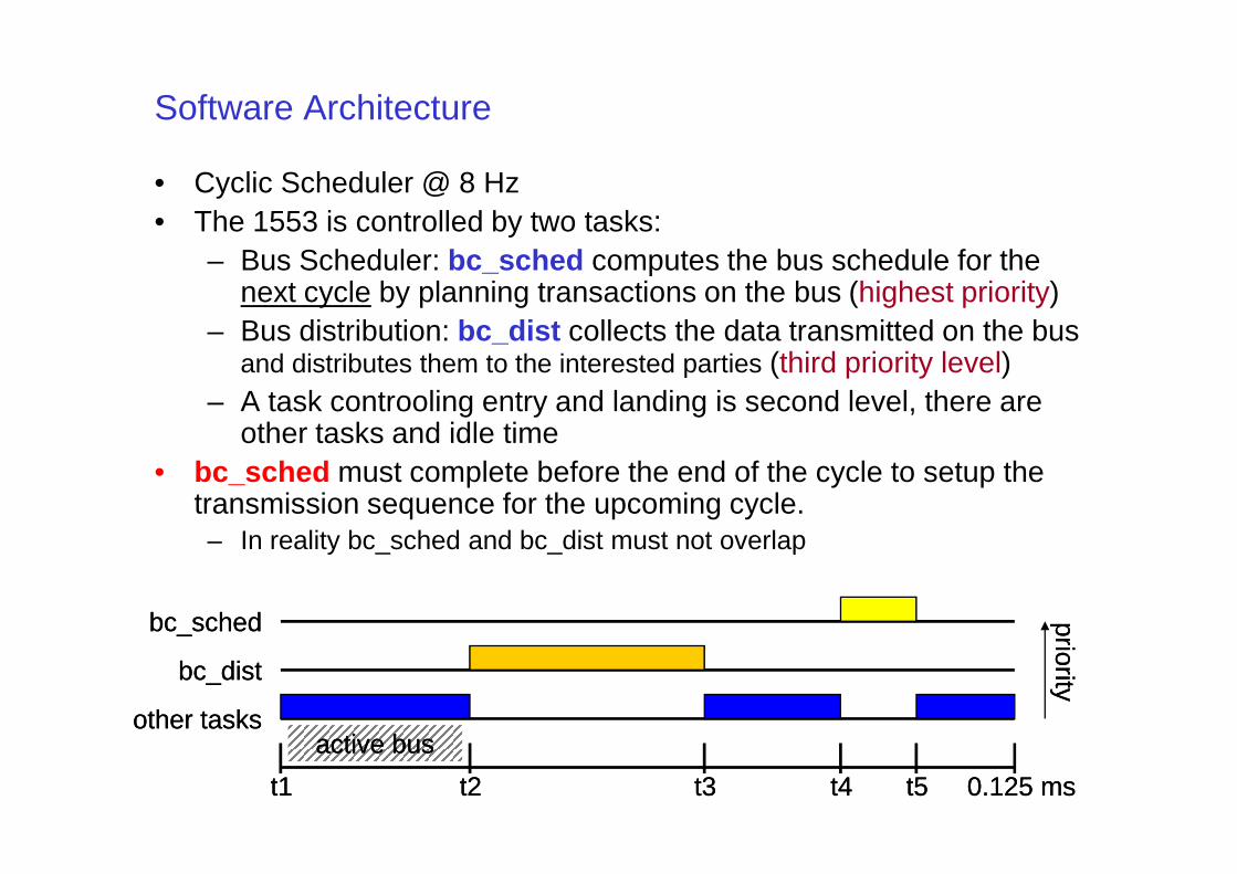
Software Architecture
• Cyclic Scheduler @ 8 Hz• The 1553 is controlled by two tasks:
– Bus Scheduler: bc_sched computes the bus schedule for the next cycle by planning transactions on the bus (highest priority)
– Bus distribution: bc_dist collects the data transmitted on the busand distributes them to the interested parties (third priority level)
– A task controoling entry and landing is second level, there are other tasks and idle timeother tasks and idle time
• bc_sched must complete before the end of the cycle to setup the transmission sequence for the upcoming cycle.– In reality bc_sched and bc_dist must not overlap
bc_distbc_dist
bc_schedbc_sched
t1t1
other tasksother tasks
0.125 ms0.125 ms
active busactive bus
t2t2 t3t3 t4t4 t5t5
prioritypriority
What happened
• The Mars Pathfinder probe lands on Mars on July 4th 1997
• After a few days the probe experiences continuous system resets as a result of a detected critical (timing) errorerror
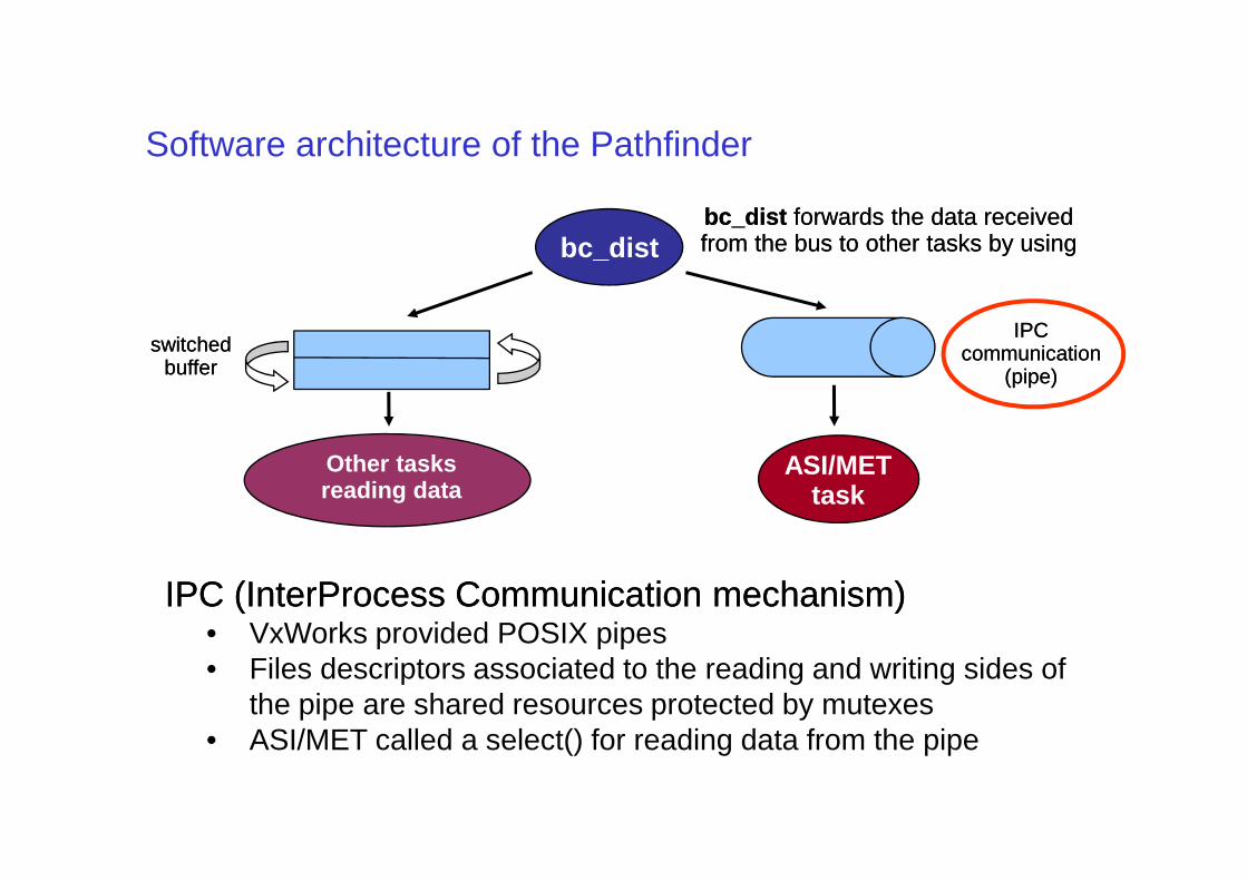
bc_distbc_dist forwards the data received forwards the data received from the bus to other tasks by usingfrom the bus to other tasks by usingbc_dist
switched switched bufferbuffer
IPC IPC communication communication
(pipe)(pipe)
Software architecture of the Pathfinder
Other tasks reading data
ASI/MET task
IPC (InterProcess Communication mechanism)IPC (InterProcess Communication mechanism)• VxWorks provided POSIX pipes• Files descriptors associated to the reading and writing sides of
the pipe are shared resources protected by mutexes• ASI/MET called a select() for reading data from the pipe
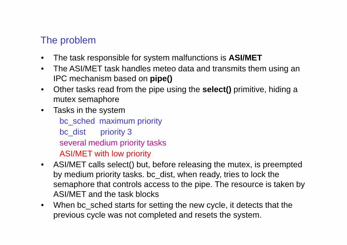
The problem
• The task responsible for system malfunctions is ASI/MET• The ASI/MET task handles meteo data and transmits them using an
IPC mechanism based on pipe()• Other tasks read from the pipe using the select() primitive, hiding a
mutex semaphore• Tasks in the system
bc_sched maximum prioritybc_sched maximum prioritybc_dist priority 3several medium priority tasksASI/MET with low priority
• ASI/MET calls select() but, before releasing the mutex, is preempted by medium priority tasks. bc_dist, when ready, tries to lock the semaphore that controls access to the pipe. The resource is taken by ASI/MET and the task blocks
• When bc_sched starts for setting the new cycle, it detects that the previous cycle was not completed and resets the system.
The problem
• The select mechanism creates a mutual exclusion semaphore to protect the "wait list" of file descriptors
• The ASI/MET task had called select, which had called pipeIoctl(), which had called selNodeAdd(), which was in the process of giving the mutex semaphore. The ASI/ MET task was preempted and semGive() was not completed.
• Several medium priority tasks ran until the bc_dist task was activated. • Several medium priority tasks ran until the bc_dist task was activated. The bc_dist task attempted to send the newest ASI/MET data via the IPC mechanism which called pipeWrite(). pipeWrite() blocked, taking the mutex semaphore. More of the medium priority tasks ran, still not allowing the ASI/MET task to run, until the bc_sched task was awakened.
• At that point, the bc_sched task determined that the bc_dist task had not completed its cycle (a hard deadline in the system) and declared the error that initiated the reset.
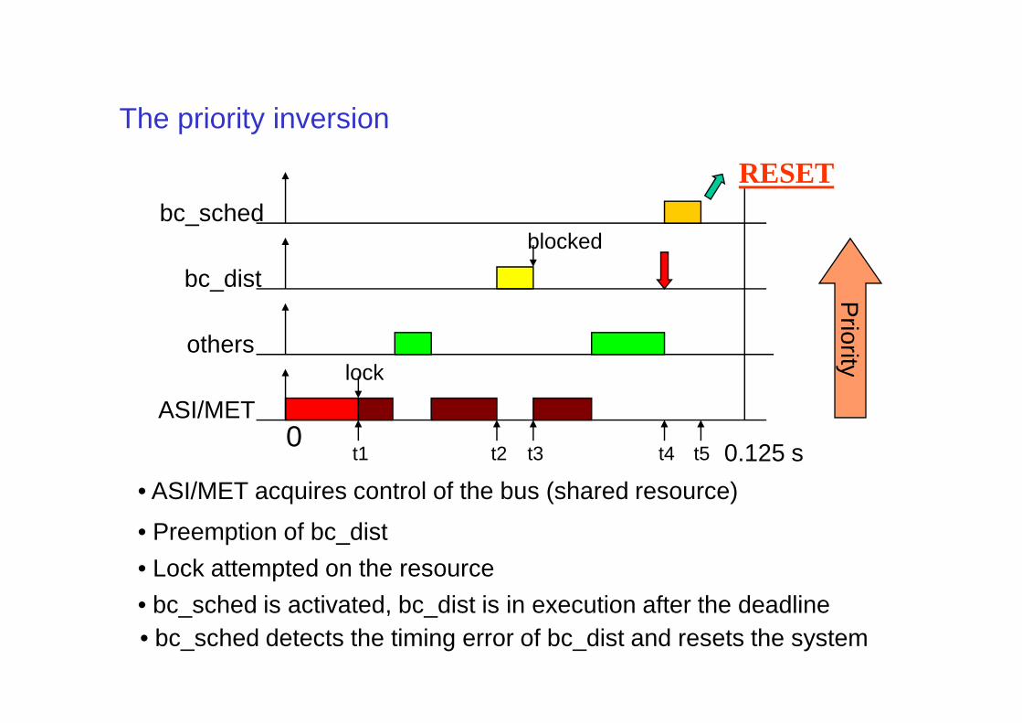
The priority inversion
bc_sched
bc_dist
others
blocked
lock
Priority
RESET
ASI/MET0
0.125 s
lock
t1 t2 t3 t4 t5
• ASI/MET acquires control of the bus (shared resource)
Priority
• Preemption of bc_dist
• Lock attempted on the resource
• bc_sched is activated, bc_dist is in execution after the deadline• bc_sched detects the timing error of bc_dist and resets the system
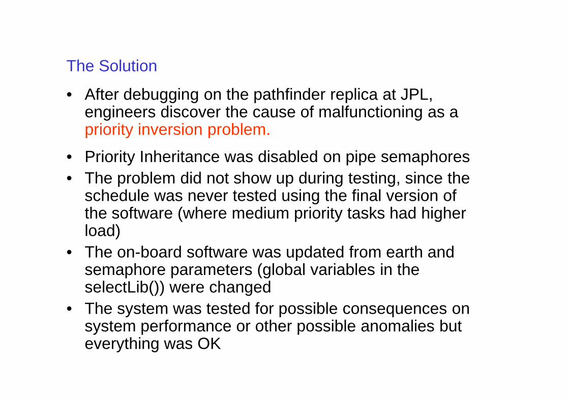
The Solution
• After debugging on the pathfinder replica at JPL, engineers discover the cause of malfunctioning as a priority inversion problem.
• Priority Inheritance was disabled on pipe semaphores• The problem did not show up during testing, since the
schedule was never tested using the final version of schedule was never tested using the final version of the software (where medium priority tasks had higher load)
• The on-board software was updated from earth and semaphore parameters (global variables in the selectLib()) were changed
• The system was tested for possible consequences on system performance or other possible anomalies but everything was OK
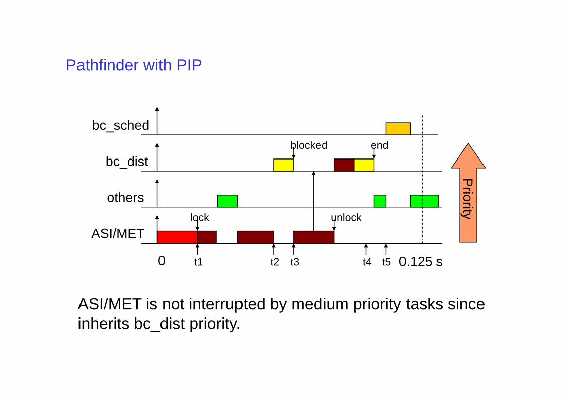
Pathfinder with PIP
bc_sched
bc_dist
others
blocked
Priority
end
others
ASI/MET
0 0.125 s
lock
t1 t2 t3 t4 t5
Priority
unlock
ASI/MET is not interrupted by medium priority tasks since inherits bc_dist priority.
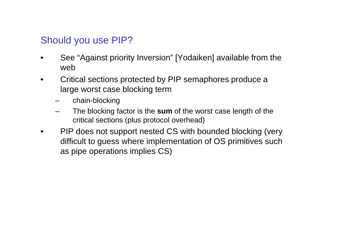
Should you use PIP?
• See “Against priority Inversion” [Yodaiken] available from the web
• Critical sections protected by PIP semaphores produce a large worst case blocking term
– chain-blocking– The blocking factor is the sum of the worst case length of the
critical sections (plus protocol overhead)critical sections (plus protocol overhead)
• PIP does not support nested CS with bounded blocking (very difficult to guess where implementation of OS primitives such as pipe operations implies CS)
• Except for very simple (but long) CS, PIP does not provide performances better then other solutions (non preemptive CS or PCP)
• PIP has a costly implementation, overheads include:– Managing the basic priority inheritance mechanism not only
requires updating the priority of the task in CS, but handling a complex data structure (not simply a stack) for storing the
Should you use PIP?
a complex data structure (not simply a stack) for storing the set of priorities inherited by each task (one list for each task and one for each mutex)
• Dynamic priority management implies dynamic reordering of the task lists
• For a full account …http://research.microsoft.com/~mbj/Mars_Pathfinder/Authoritative_Account.html
Specifications
Software design
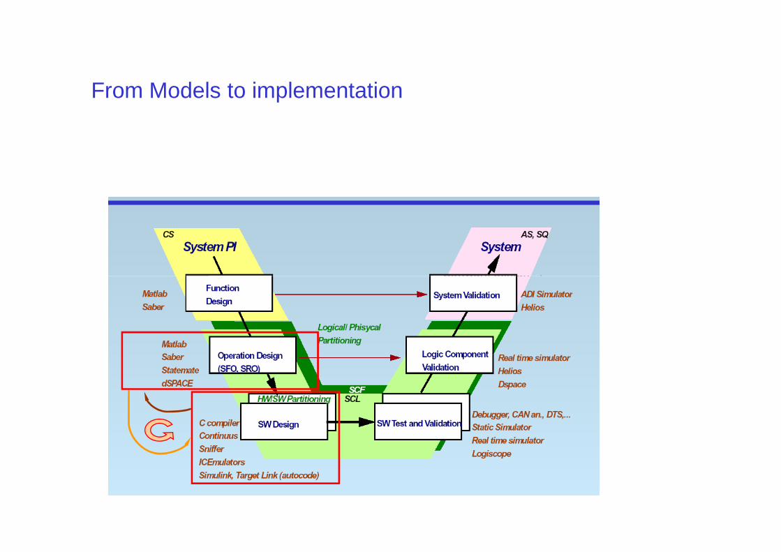
From Models to implementation
Control algorithmdesign
Control designsign-off
Software design
Functionaltesting
Software designsign-off
From Models to implementation
• Keeping the code semantics aligned with model• if code is automatically produced then correct
implementation should be guaranteed … (or not?) • We will consider the Simulink case• Beware of concurrent implementation (access to • Beware of concurrent implementation (access to
shared variables may introduce nondeterminism)
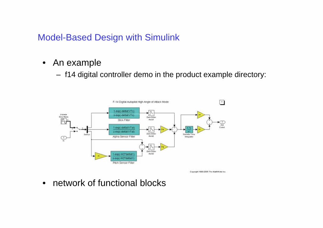
Model-Based Design with Simulink
• An example – f14 digital controller demo in the product example directory:
• network of functional blocks
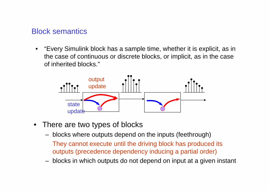
Block semantics
• “Every Simulink block has a sample time, whether it is explicit, as in the case of continuous or discrete blocks, or implicit, as in the case of inherited blocks.”
output update
• There are two types of blocks– blocks where outputs depend on the inputs (feethrough)
They cannot execute until the driving block has produced its outputs (precedence dependency inducing a partial order)
– blocks in which outputs do not depend on input at a given instant
state update
From Models to implementation
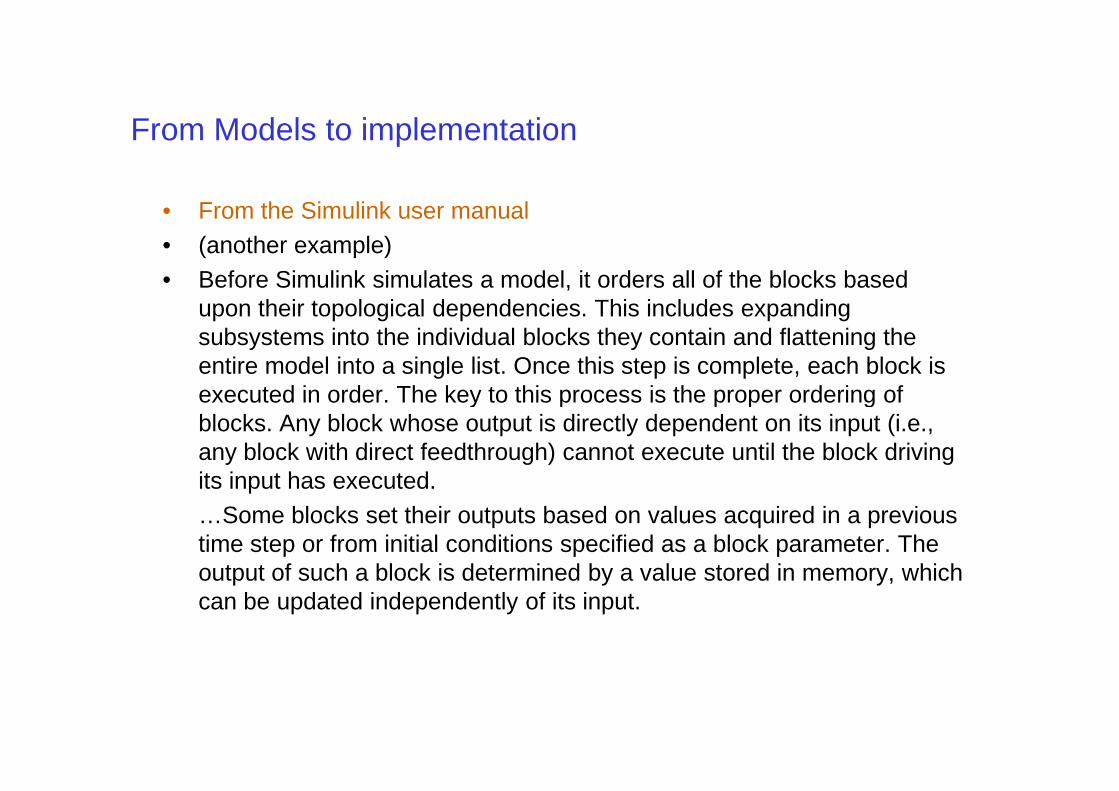
• From the Simulink user manual• (another example)• Before Simulink simulates a model, it orders all of the blocks based
upon their topological dependencies. This includes expanding subsystems into the individual blocks they contain and flattening the entire model into a single list. Once this step is complete, each block is executed in order. The key to this process is the proper ordering of executed in order. The key to this process is the proper ordering of blocks. Any block whose output is directly dependent on its input (i.e., any block with direct feedthrough) cannot execute until the block driving its input has executed.…Some blocks set their outputs based on values acquired in a previous time step or from initial conditions specified as a block parameter. The output of such a block is determined by a value stored in memory, which can be updated independently of its input.
Simulink+RTW: Execution order of blocks
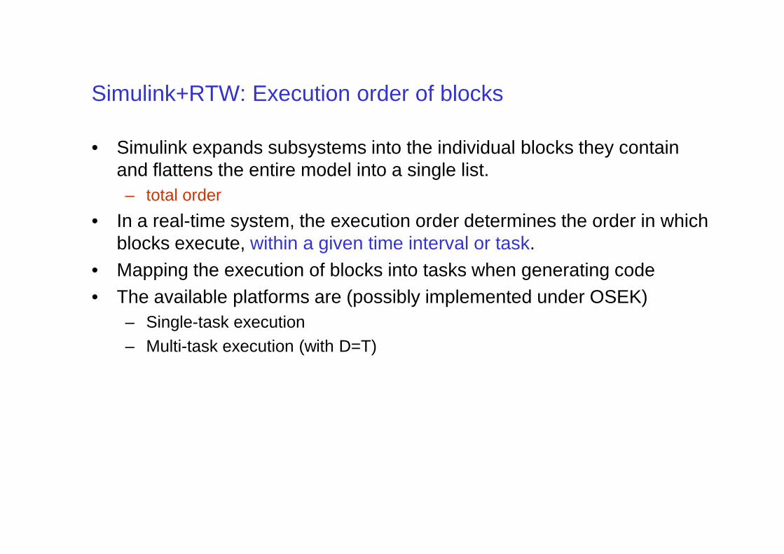
• Simulink expands subsystems into the individual blocks they contain and flattens the entire model into a single list. – total order
• In a real-time system, the execution order determines the order in which blocks execute, within a given time interval or task.
• Mapping the execution of blocks into tasks when generating code• Mapping the execution of blocks into tasks when generating code• The available platforms are (possibly implemented under OSEK)
– Single-task execution– Multi-task execution (with D=T)
Simulation of models
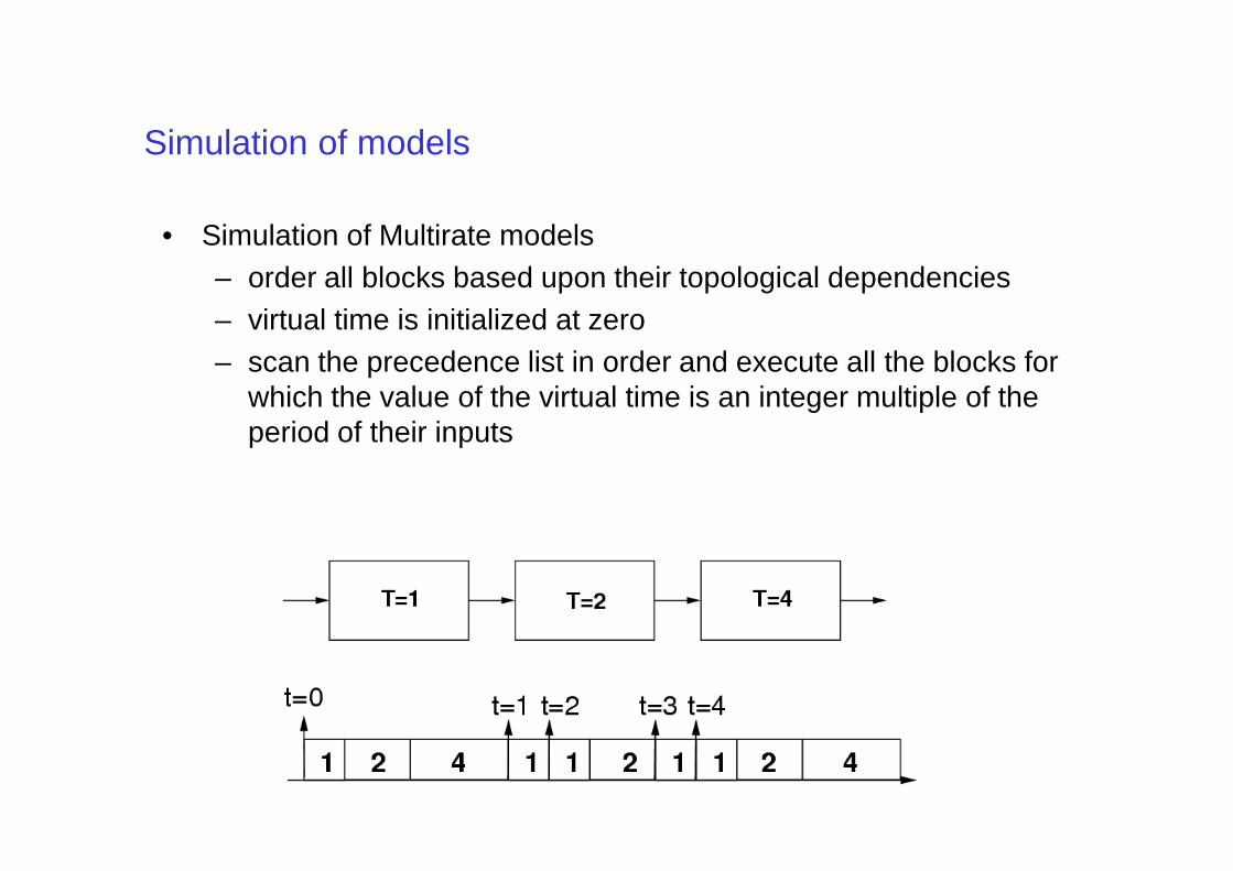
• Simulation of Multirate models– order all blocks based upon their topological dependencies– virtual time is initialized at zero– scan the precedence list in order and execute all the blocks for
which the value of the virtual time is an integer multiple of the period of their inputsperiod of their inputs
Implementation of models
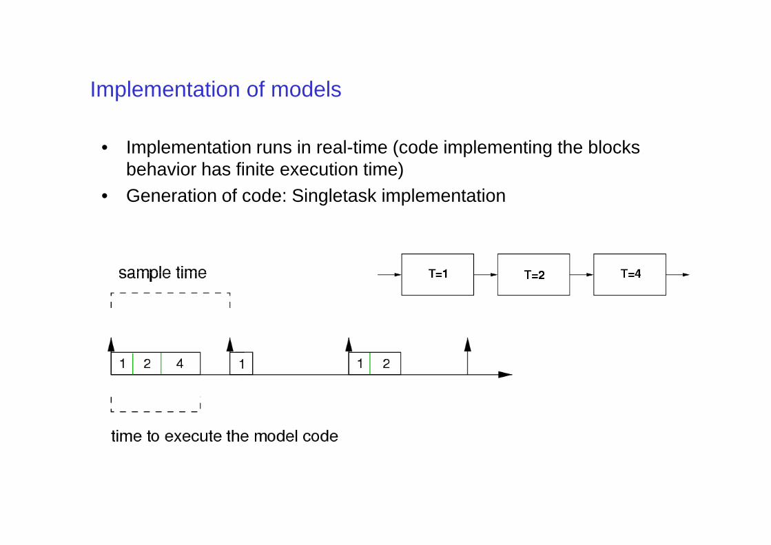
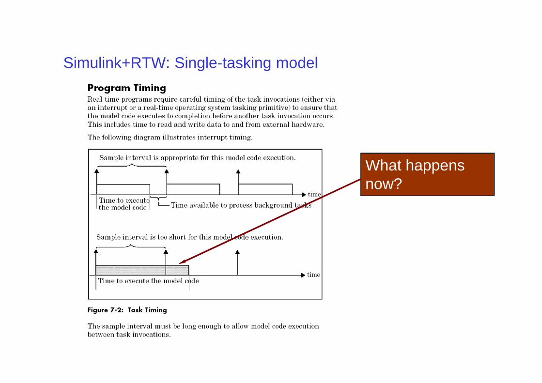
• Implementation runs in real-time (code implementing the blocks behavior has finite execution time)
• Generation of code: Singletask implementation
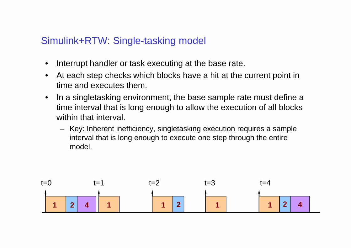
• Interrupt handler or task executing at the base rate.• At each step checks which blocks have a hit at the current point in
time and executes them.• In a singletasking environment, the base sample rate must define a
time interval that is long enough to allow the execution of all blocks within that interval.
Simulink+RTW: Single-tasking model
– Key: Inherent inefficiency, singletasking execution requires a sample interval that is long enough to execute one step through the entire model.
t=0 t=1 t=2 t=3 t=4
1 1 1 1 12 2 24 4
From Models to implementation
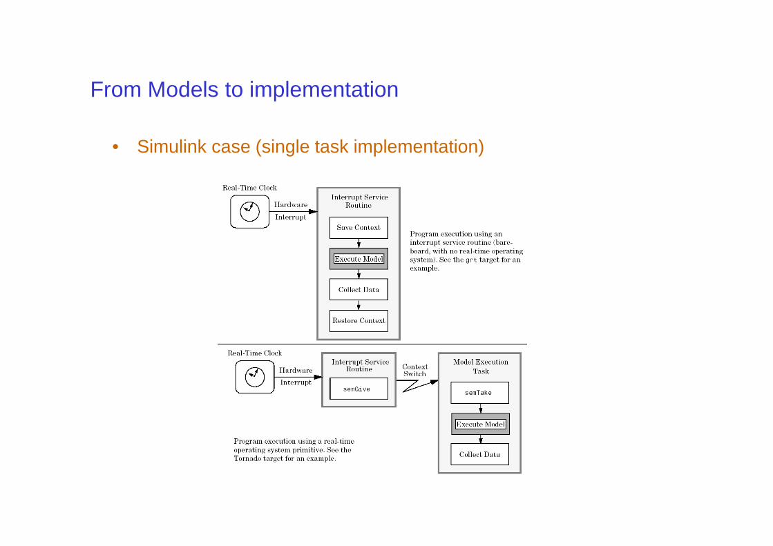
• Simulink case (single task implementation)
Simulink+RTW: Single-tasking model
What happens now?now?
• Executing code in the context of a real-time thread– if the model has blocks with different sample rates, the code assigns
each block a task identifier (tid) to associate the block with the task that executes at the block’s sample rate.
– There is one task/thread for each rate and the code implementing the block is executed according to the global order determined by Simulink
• Priority order
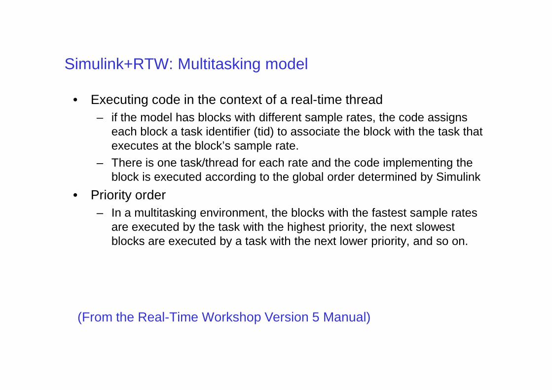
Simulink+RTW: Multitasking model
• Priority order– In a multitasking environment, the blocks with the fastest sample rates
are executed by the task with the highest priority, the next slowest blocks are executed by a task with the next lower priority, and so on.
(From the Real-Time Workshop Version 5 Manual)
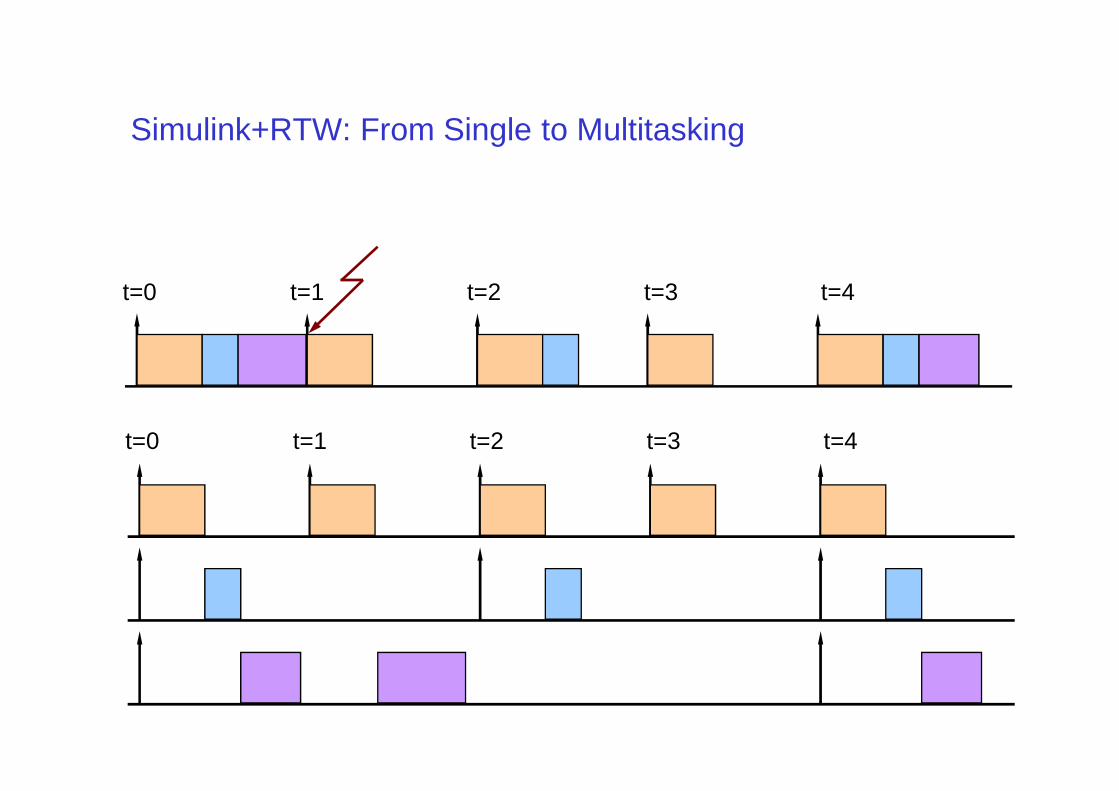
Simulink+RTW: From Single to Multitasking
t=0 t=1 t=2 t=3 t=4
t=0 t=1 t=2 t=3 t=4
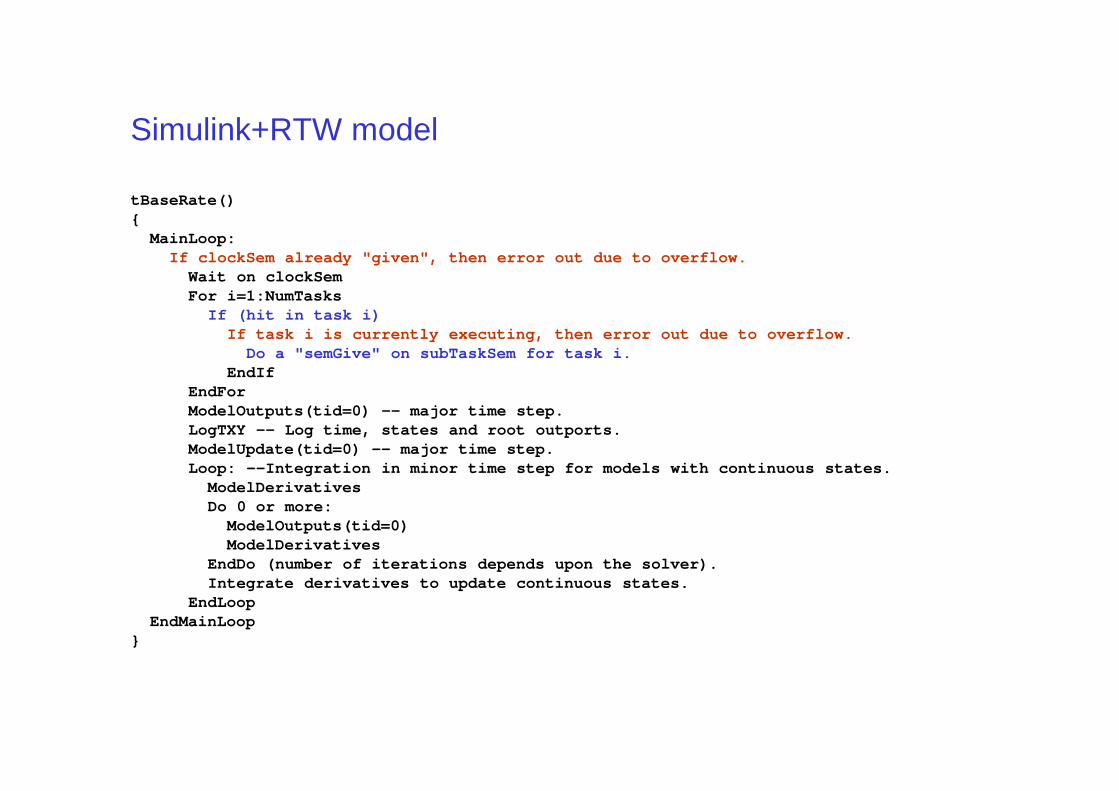
Simulink+RTW model
tBaseRate(){MainLoop:
If clockSem already "given", then error out due to overflow.Wait on clockSemFor i=1:NumTasks
If (hit in task i)If task i is currently executing, then error out due to overflow.
Do a "semGive" on subTaskSem for task i.EndIf
EndForEndForModelOutputs(tid=0) -- major time step.LogTXY -- Log time, states and root outports.ModelUpdate(tid=0) -- major time step.Loop: --Integration in minor time step for models with continuous states.
ModelDerivativesDo 0 or more:
ModelOutputs(tid=0)ModelDerivatives
EndDo (number of iterations depends upon the solver).Integrate derivatives to update continuous states.
EndLoopEndMainLoop
}
From Models to implementation
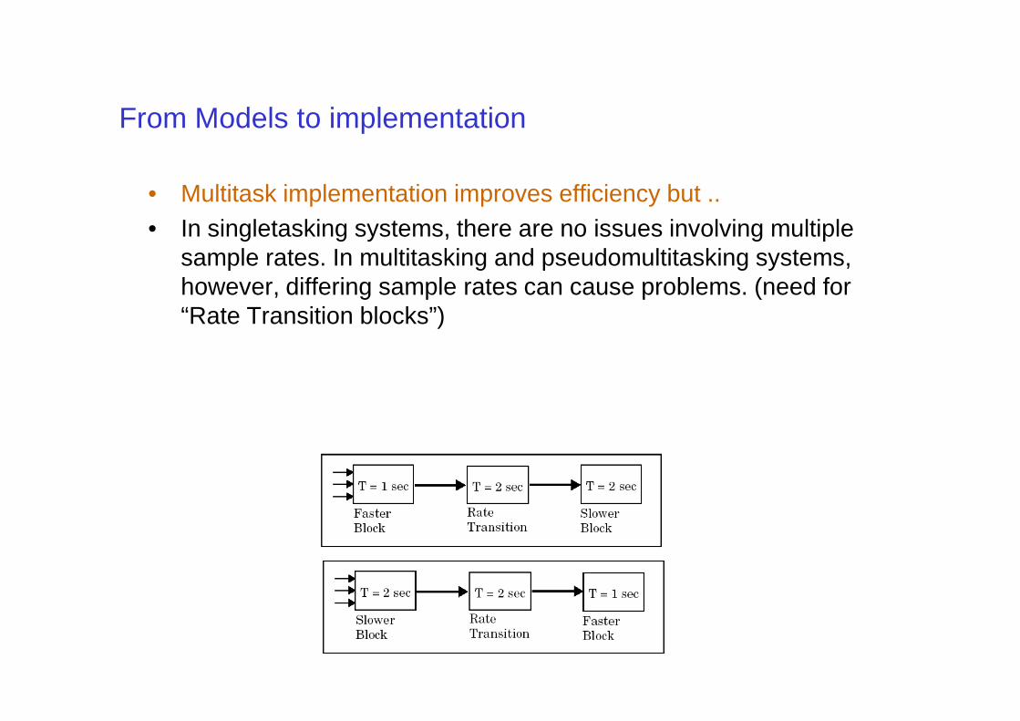
• Multitask implementation improves efficiency but ..• In singletasking systems, there are no issues involving multiple
sample rates. In multitasking and pseudomultitasking systems, however, differing sample rates can cause problems. (need for “Rate Transition blocks”)
From Models to implementation
• What is the purpose of a data transition block?• Given the user control upon:
– Data integrity (option on/off (!))– Deterministic vs. nondeterministic transfer
• Deterministic transfer has maximum delay• Deterministic transfer has maximum delay• Protected/Deterministic (default) is the safest mode.
The drawback of this mode is that it introduces latency into the system:– Fast to slow transition: maximum latency is 1 sample period
of the slower task.– Slow to fast transition: maximum latency is 2 sample periods
of the slower task.
Nondeterminism in both time and value
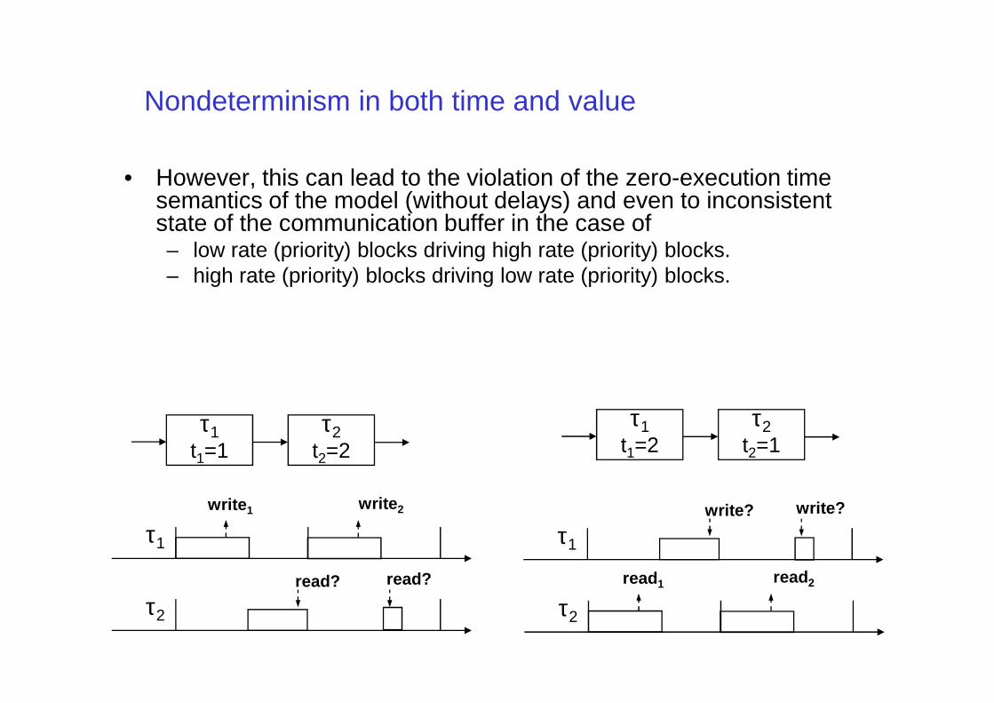
• However, this can lead to the violation of the zero-execution time semantics of the model (without delays) and even to inconsistent state of the communication buffer in the case of – low rate (priority) blocks driving high rate (priority) blocks.– high rate (priority) blocks driving low rate (priority) blocks.
τ1t1=1
τ2t2=2
τ1t1=2
τ2t2=1
τ1
write1 write2
τ2
read? read?
τ2
read1 read2
τ1
write? write?
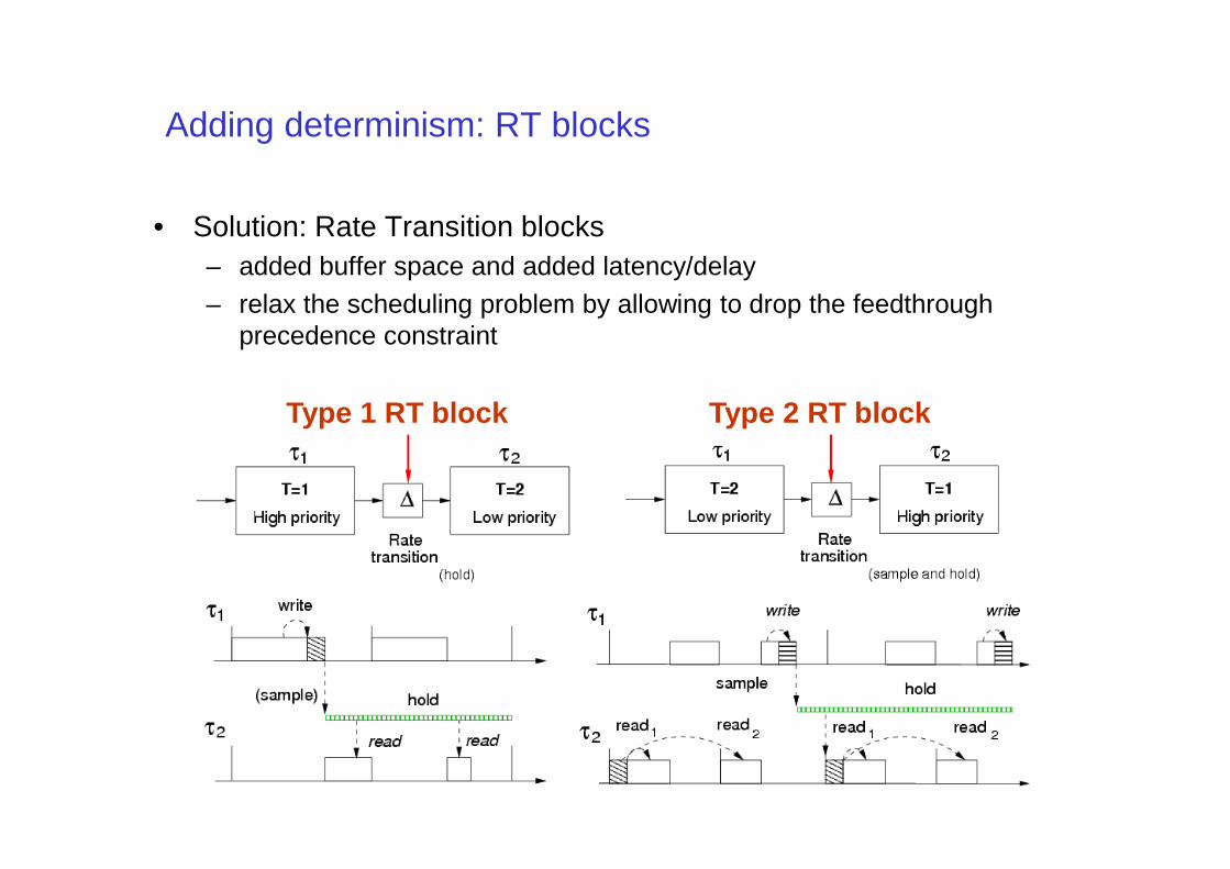
Adding determinism: RT blocks
• Solution: Rate Transition blocks– added buffer space and added latency/delay– relax the scheduling problem by allowing to drop the feedthrough
precedence constraint
Type 1 RT block Type 2 RT block
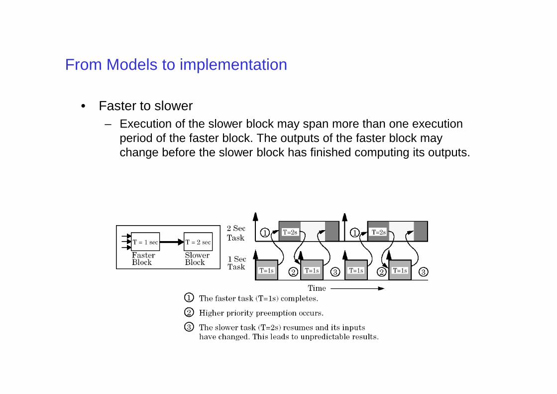
From Models to implementation
• Faster to slower– Execution of the slower block may span more than one execution
period of the faster block. The outputs of the faster block may change before the slower block has finished computing its outputs.
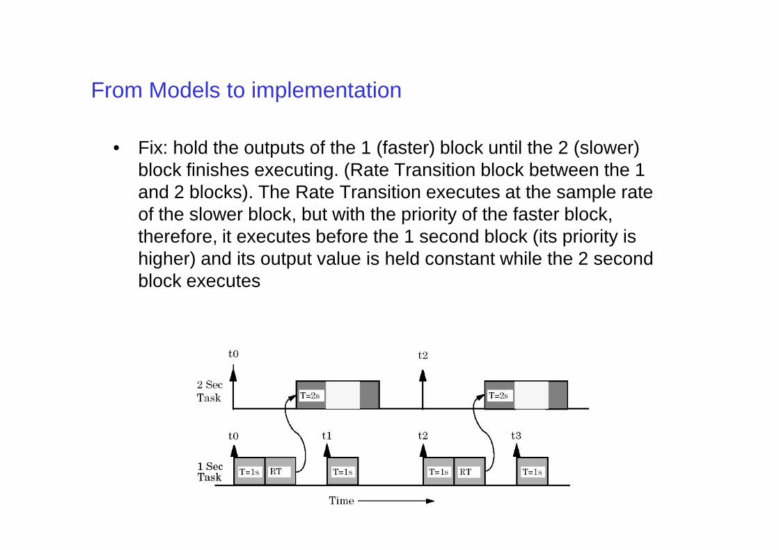
From Models to implementation
• Fix: hold the outputs of the 1 (faster) block until the 2 (slower) block finishes executing. (Rate Transition block between the 1 and 2 blocks). The Rate Transition executes at the sample rate of the slower block, but with the priority of the faster block, therefore, it executes before the 1 second block (its priority is higher) and its output value is held constant while the 2 second block executesblock executes
From Models to implementation
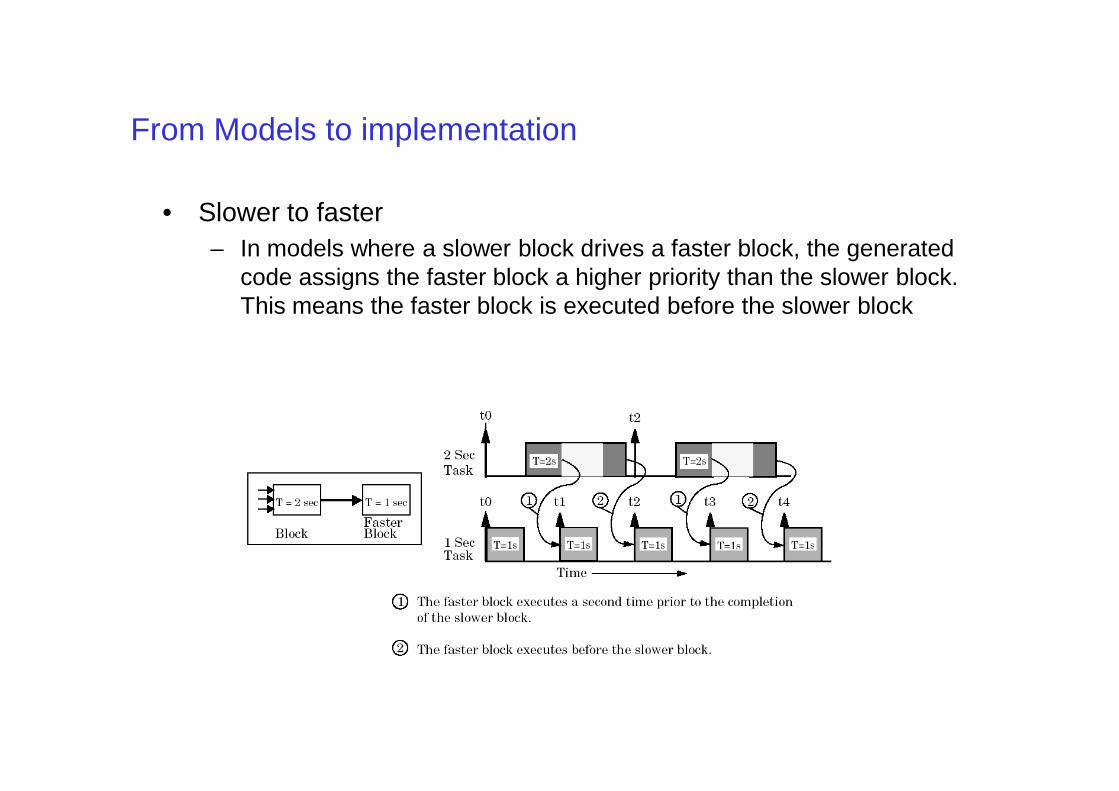
• Slower to faster– In models where a slower block drives a faster block, the generated
code assigns the faster block a higher priority than the slower block. This means the faster block is executed before the slower block
From Models to implementation
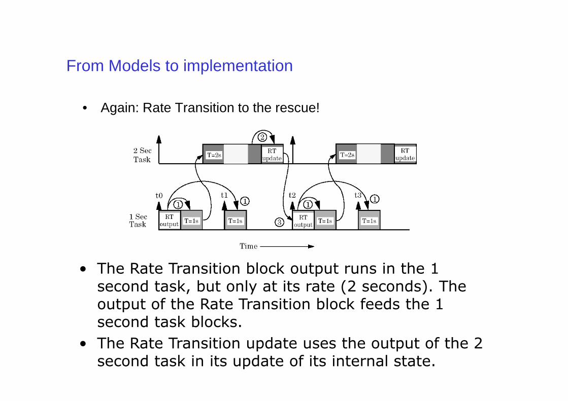
• Again: Rate Transition to the rescue!
• The Rate Transition block output runs in the 1 second task, but only at its rate (2 seconds). The output of the Rate Transition block feeds the 1 second task blocks.
• The Rate Transition update uses the output of the 2 second task in its update of its internal state.
From Models to implementation
• The Rate Transition update uses the state of the Rate Transition in the 1 second task.
• The output portion of a Rate Transition block is executed at the sample rate of the slower block, but with the priority of the faster block. Since the Rate Transition block drives the faster block and has effectively the same priority, it is executed before the faster block. This solves the first problem.
• The second problem is alleviated (!) because the Rate Transition block • The second problem is alleviated (!) because the Rate Transition block executes at a slower rate and its output does not change during the computation of the faster block it is driving.
OSEK/VDX?
• a standard for an open-ended architecture for distributed control units in vehicles
• the name:– OSEK: Offene Systeme und deren Schnittstellen für die
Elektronik im Kraft-fahrzeug (Open systems and the corresponding interfaces for automotive electronics)
– VDX: Vehicle Distributed eXecutive (another french proposal – VDX: Vehicle Distributed eXecutive (another french proposal of API similar to OSEK)
– OSEK/VDX is the interface resulted from the merge of the two projects
• http://www.osek-vdx.org
motivations
• high, recurring expenses in the development and variant management of non-application related aspectsof control unit software.
• incompatibility of control units made by different manufacturers due to different interfaces and protocols
objectives
• portability and reusability of the application software • specification of abstract interfaces for RTOS and
network management• specification independent from the HW/network details• scalability between different requirements to adapt to
particular application needsparticular application needs• verification of functionality and implementation using a
standardized certification process
advantages
• clear savings in costs and development time. • enhanced quality of the software• creation of a market of uniform competitors• independence from the implementation and
standardised interfacing features for control units with different architectural designsdifferent architectural designs
• intelligent usage of the hardware present on the vehicle– for example, using a vehicle network the ABS controller could
give a speed feedback to the powertrain microcontroller
system philosophy
• standard interface ideal for automotive applications
• scalability– using conformance classes
• configurable error checking • configurable error checking
• portability of software– in reality, the firmware on an automotive ECU is 10% RTOS
and 90% device drivers
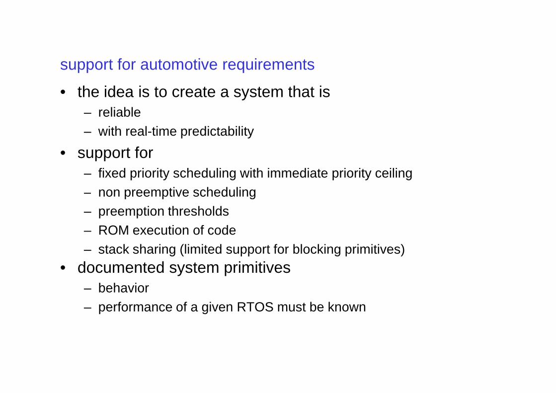
support for automotive requirements
• the idea is to create a system that is– reliable– with real-time predictability
• support for – fixed priority scheduling with immediate priority ceiling– non preemptive scheduling– non preemptive scheduling– preemption thresholds– ROM execution of code– stack sharing (limited support for blocking primitives)
• documented system primitives– behavior– performance of a given RTOS must be known
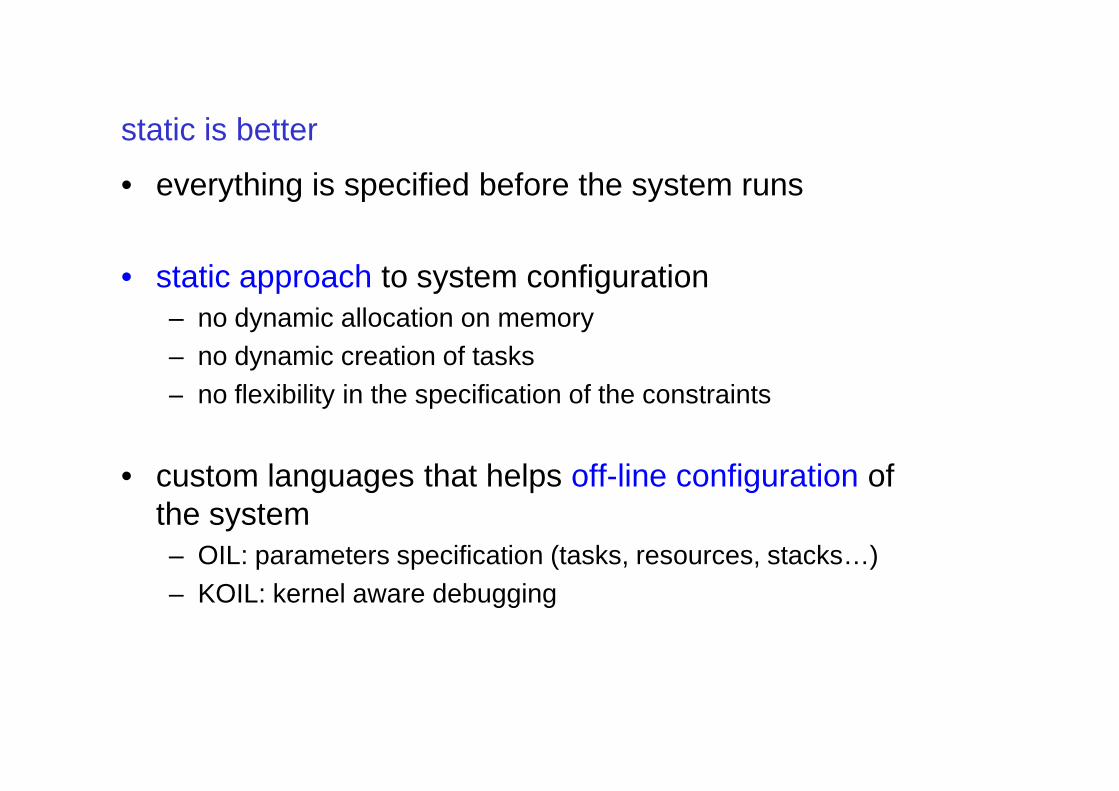
static is better
• everything is specified before the system runs
• static approach to system configuration– no dynamic allocation on memory– no dynamic creation of tasks– no flexibility in the specification of the constraints– no flexibility in the specification of the constraints
• custom languages that helps off-line configuration of the system– OIL: parameters specification (tasks, resources, stacks…)– KOIL: kernel aware debugging
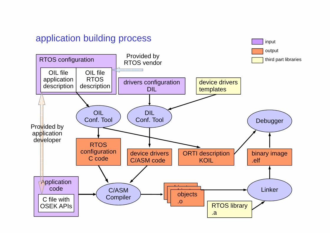
application building process
RTOS configuration
drivers configurationDIL
OILConf. Tool
device driverstemplates
DILConf. Tool
input
output
third part libraries
OIL file application description
OIL file RTOS
description
Provided by RTOS vendor
Application code
RTOS library.a
device driversC/ASM code
Conf. Tool
C/ASMCompiler
RTOS configuration
C codeORTI description
KOIL
Linker
Debugger
objects.oobjects.oobjects.o
Conf. Tool
binary image.elf
C file with OSEK APIs
Provided by application developer
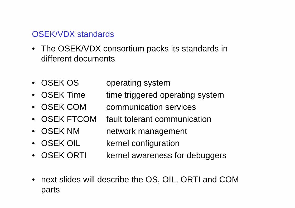
OSEK/VDX standards
• The OSEK/VDX consortium packs its standards in different documents
• OSEK OS operating system• OSEK Time time triggered operating system• OSEK COM communication services• OSEK COM communication services• OSEK FTCOM fault tolerant communication• OSEK NM network management• OSEK OIL kernel configuration• OSEK ORTI kernel awareness for debuggers
• next slides will describe the OS, OIL, ORTI and COM parts
processing levels
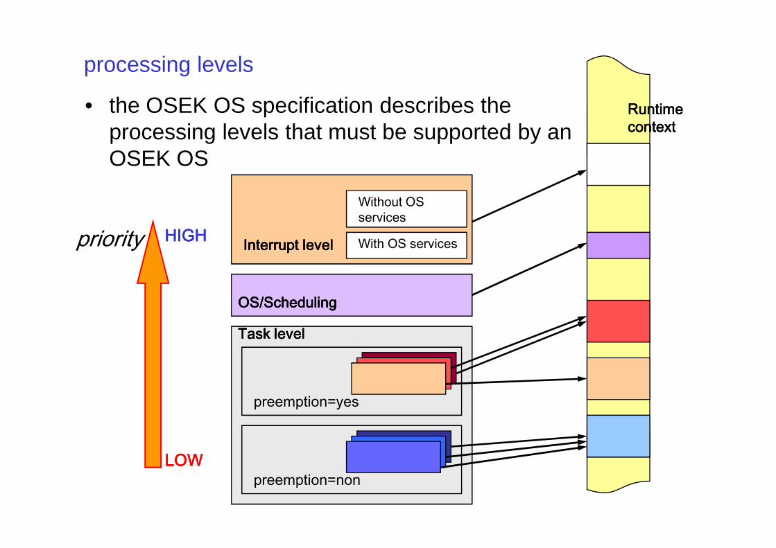
• the OSEK OS specification describes the processing levels that must be supported by an OSEK OS
priority HIGHHIGHHIGHHIGH Interrupt levelInterrupt levelInterrupt levelInterrupt level
Runtime Runtime Runtime Runtime contextcontextcontextcontext
With OS services
Without OS services
LOWLOWLOWLOW
Task levelTask levelTask levelTask level
preemption=non
OS/SchedulingOS/SchedulingOS/SchedulingOS/Scheduling
preemption=yes
conformance classes
• OSEK OS should be scalable with the application needs– different applications require different services– the system services are mapped in Conformance Classes
• a conformance class is a subset of the OSEK OS standardstandard
• objectives of the conformance classes– allow partial implementation of the standard– allow an upgrade path between classes
• services that discriminates the different conformance classes– multiple requests of task activations– task types– number of tasks per priority
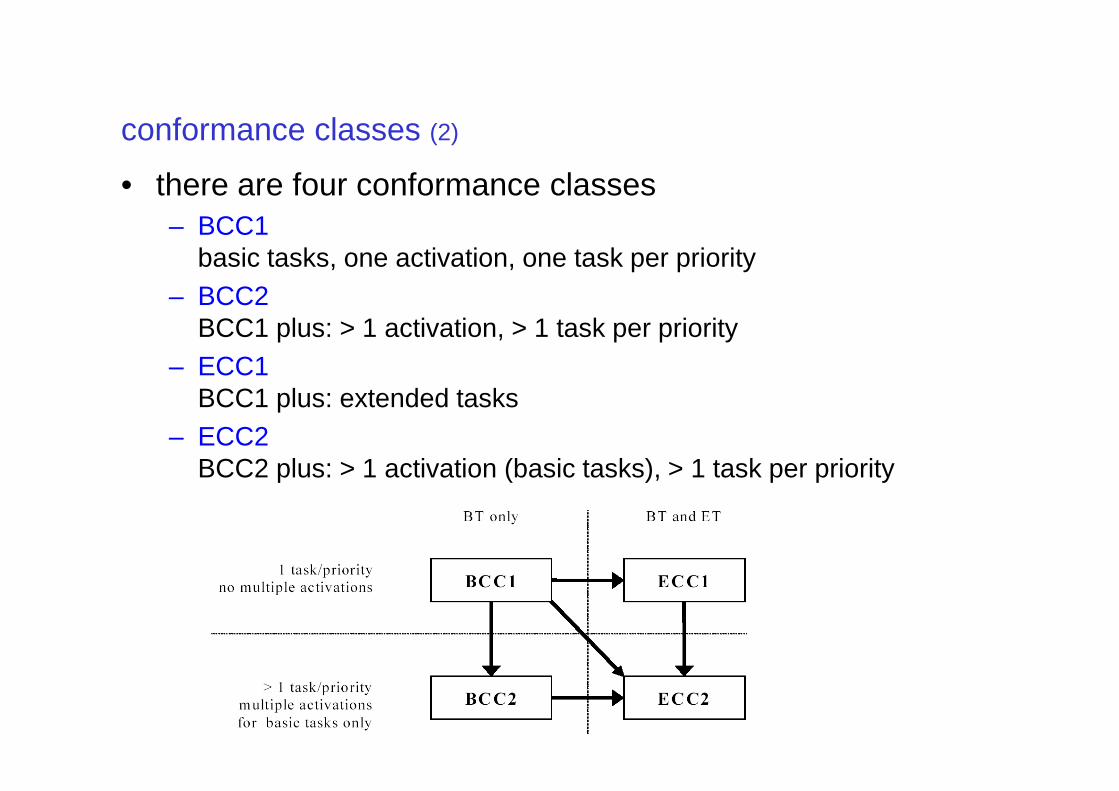
conformance classes (2)
• there are four conformance classes– BCC1
basic tasks, one activation, one task per priority– BCC2
BCC1 plus: > 1 activation, > 1 task per priority– ECC1
BCC1 plus: extended tasksBCC1 plus: extended tasks– ECC2
BCC2 plus: > 1 activation (basic tasks), > 1 task per priority
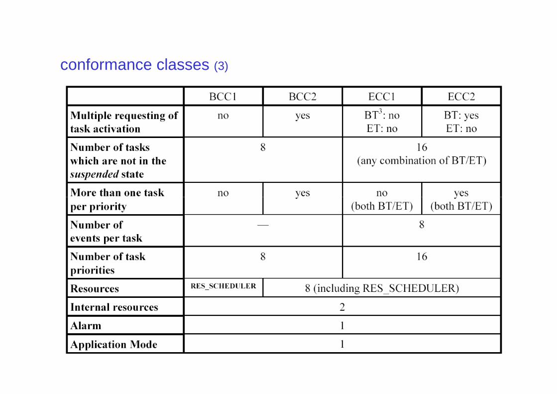
conformance classes (3)
basic tasks
• a basic task is – a C function call that is executed in a proper context– that can never block– can lock resources– can only finish or be preempted by an higher priority task or
ISR
• a basic task is ideal for implementing a kernel-• a basic task is ideal for implementing a kernel-supported stack sharing, because– the task never blocks– when the function call ends, the task ends, and its local
variables are destroyed– in other words, it uses a one-shot task model
• support for multiple activations– in BCC2, ECC2, basic tasks can store pending activations (a
task can be activated while it is still running)
extended tasks
• extended tasks can use events for synchronization• an event is simply an abstraction of a bit mask
– events can be set/reset using appropriate primitives– a task can wait for an event in event mask to be set
• extended tasks typically– have its own stack– have its own stack– are activated once– have as body an infinite loop over a WaitEvent() primitive
• extended tasks do not support for multiple activations– ... but supports multiple pending events
scheduling algorithm
• the scheduling algorithm is fundamentally a – fixed priority scheduler– with immediate priority ceiling– with preemption threshold
• the approach allows the implementation of– preemptive scheduling– preemptive scheduling– non preemptive scheduling– mixed
• with some peculiarities...
scheduling algorithm: peculiarities
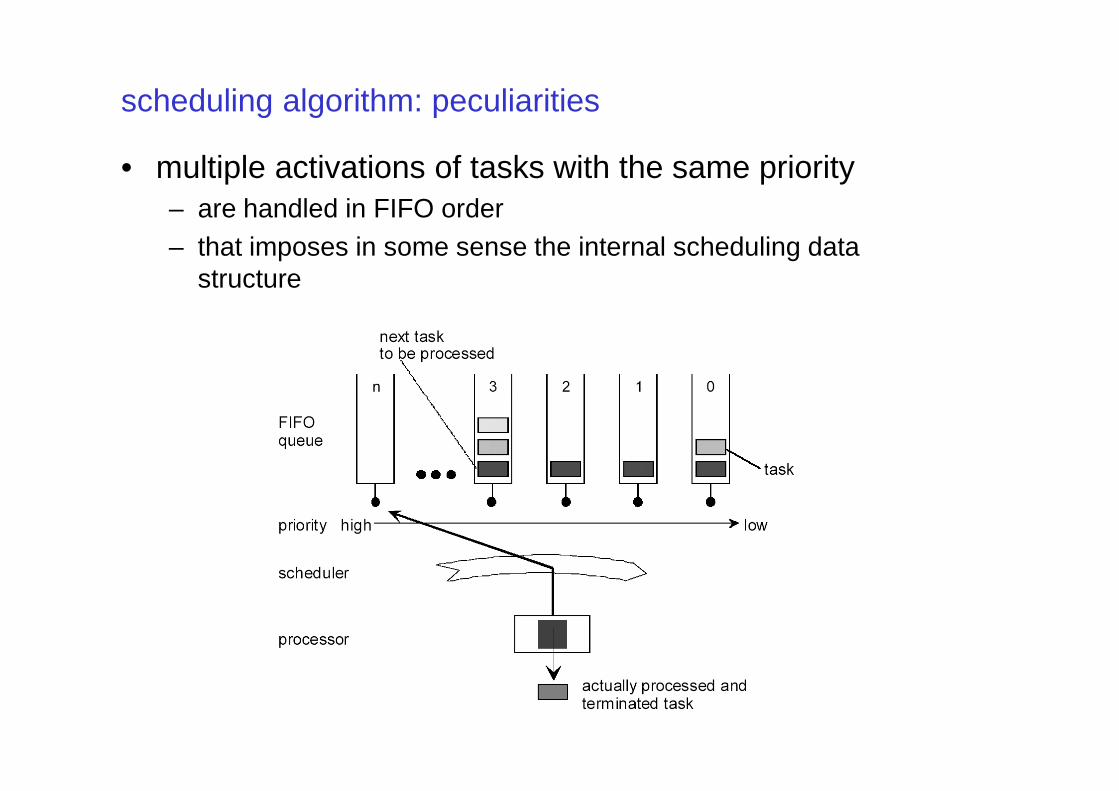
• multiple activations of tasks with the same priority– are handled in FIFO order– that imposes in some sense the internal scheduling data
structure
scheduling algorithm: peculiarities (2)
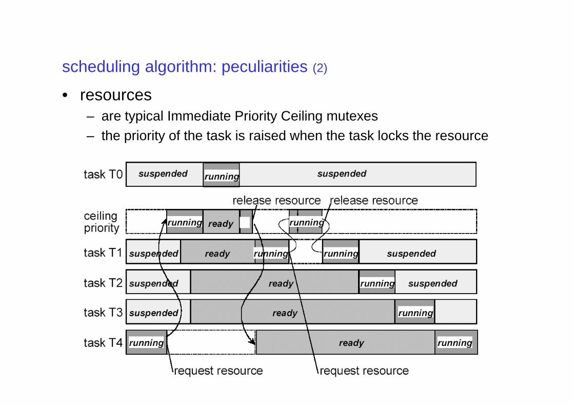
• resources– are typical Immediate Priority Ceiling mutexes– the priority of the task is raised when the task locks the resource
scheduling algorithm: peculiarities (3)
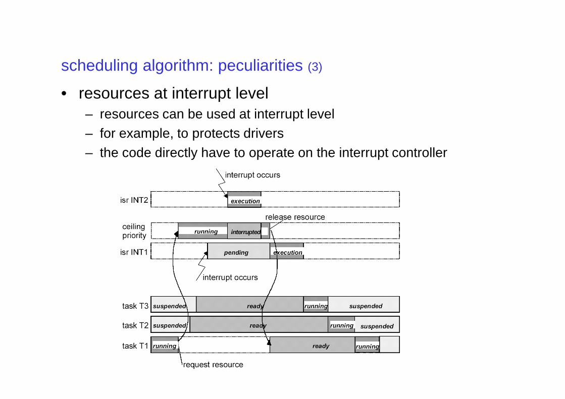
• resources at interrupt level– resources can be used at interrupt level– for example, to protects drivers– the code directly have to operate on the interrupt controller
scheduling algorithm: peculiarities (4)
• preemption threshold implementation– done using “internal resources” that are locked when the task
starts and unlocked when the task ends– internal resources cannot be used by the application
interrupt service routine
• OSEK OS directly addresses interrupt management in the standard API
• interrupt service routines (ISR) can be of two types– Category 1: without API calls
simpler and faster, do not implement a call to the scheduler at the end of the ISR
– Category 2: with API callsthese ISR can call some primitives (ActivateTask, ...) that change the scheduling behavior. The end of the ISR is a rescheduling point
• ISR 1 has always a higher priority of ISR 2
• finally, the OSEK standard has functions to directly manipulate the CPU interrupt status
counters and alarms
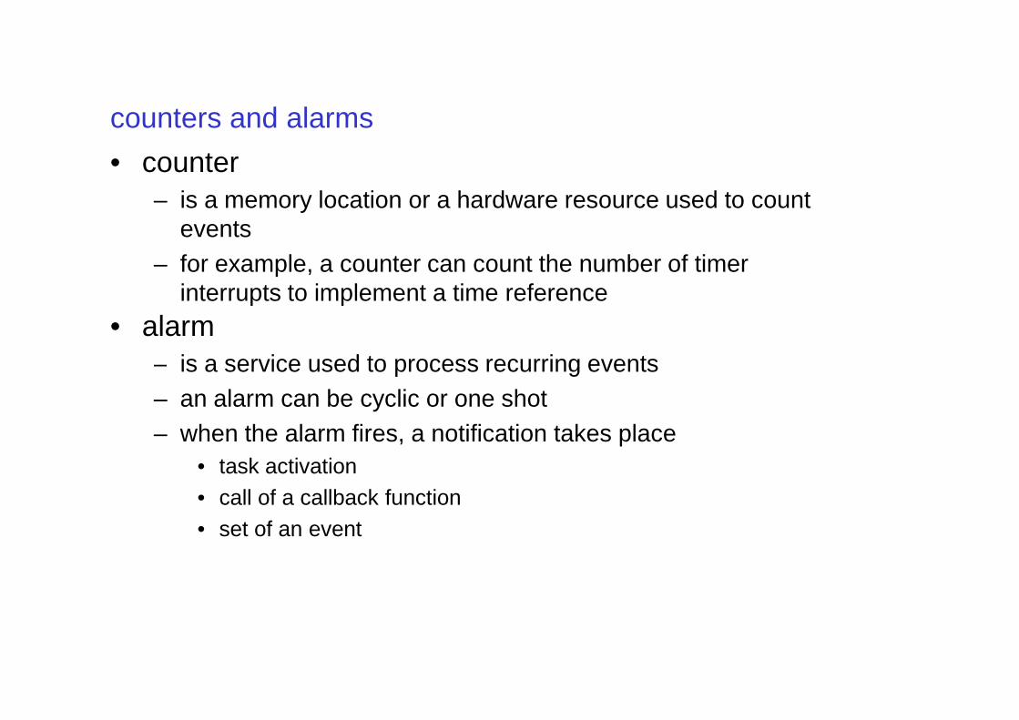
• counter– is a memory location or a hardware resource used to count
events– for example, a counter can count the number of timer
interrupts to implement a time reference• alarm
– is a service used to process recurring events– is a service used to process recurring events– an alarm can be cyclic or one shot– when the alarm fires, a notification takes place
• task activation• call of a callback function• set of an event
application modes
• OSEK OS supports the concept of application modes• an application mode is used to influence the behavior
of the device• example of application modes
– normal operation– debug mode– debug mode– diagnostic mode– ...
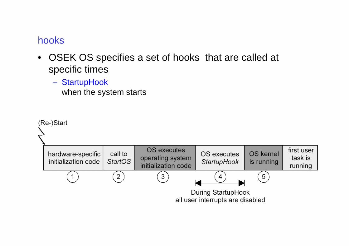
hooks
• OSEK OS specifies a set of hooks that are called at specific times– StartupHook
when the system starts
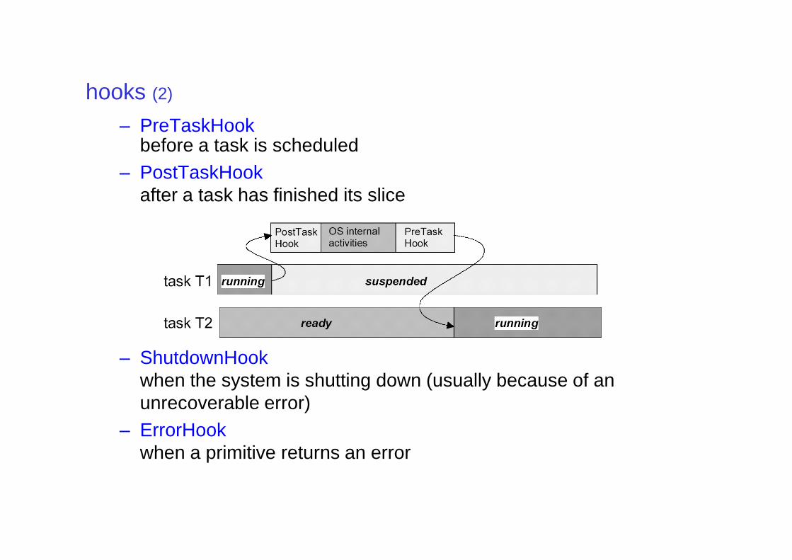
hooks (2)
– PreTaskHookbefore a task is scheduled
– PostTaskHookafter a task has finished its slice
– ShutdownHookwhen the system is shutting down (usually because of an unrecoverable error)
– ErrorHookwhen a primitive returns an error
error handling
• the OSEK OS has two types or error return values– standard error
(only errors related to the runtime behavior are returned)– extended error
(more errors are returned, useful when debugging)
• the user have two ways of handling these errors– distributed error checking– distributed error checking
the user checks the return value of each primitive– centralized error checking
the user provides a ErrorHook that is called whenever an error condition occurs
OSEK OIL
• goal– provide a mechanism to configure an OSEK application inside
a particular CPU (for each CPU there is one OIL description)
• the OIL language– allows the user to define objects with properties
(e.g., a task that has a priority)– some object and properties have a behavior specified by the
standard
• an OIL file is divided in two parts– an implementation definition
defines the objects that are present and their properties– an application definition
define the instances of the available objects for a given application
OSEK OIL objects
• The OIL specification defines the properties of the following objects:– CPU
the CPU on which the application runs– OS
the OSEK OS which runs on the CPU– ISR– ISR
interrupt service routines supported by OS– RESOURCE
the resources which can be occupied by a task– TASK
the task handled by the OS– COUNTER
the counter represents hardware/software tick source for alarms.
OSEK OIL objects (2)
– EVENTthe event owned by a task. A
– ALARMthe alarm is based on a counter
– MESSAGEthe COM message which provides local or network communication
– COMthe communication subsystem
– NMthe network management subsystem
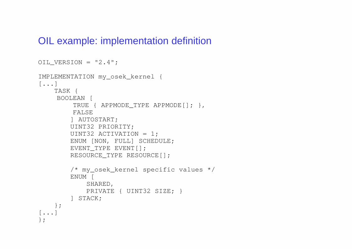
OIL example: implementation definition
OIL_VERSION = "2.4";
IMPLEMENTATION my_osek_kernel {[...]
TASK {BOOLEAN [
TRUE { APPMODE_TYPE APPMODE[]; },FALSE
] AUTOSTART;UINT32 PRIORITY;UINT32 PRIORITY;UINT32 ACTIVATION = 1;ENUM [NON, FULL] SCHEDULE;EVENT_TYPE EVENT[];RESOURCE_TYPE RESOURCE[];
/* my_osek_kernel specific values */ENUM [
SHARED,PRIVATE { UINT32 SIZE; }
] STACK;};
[...]};
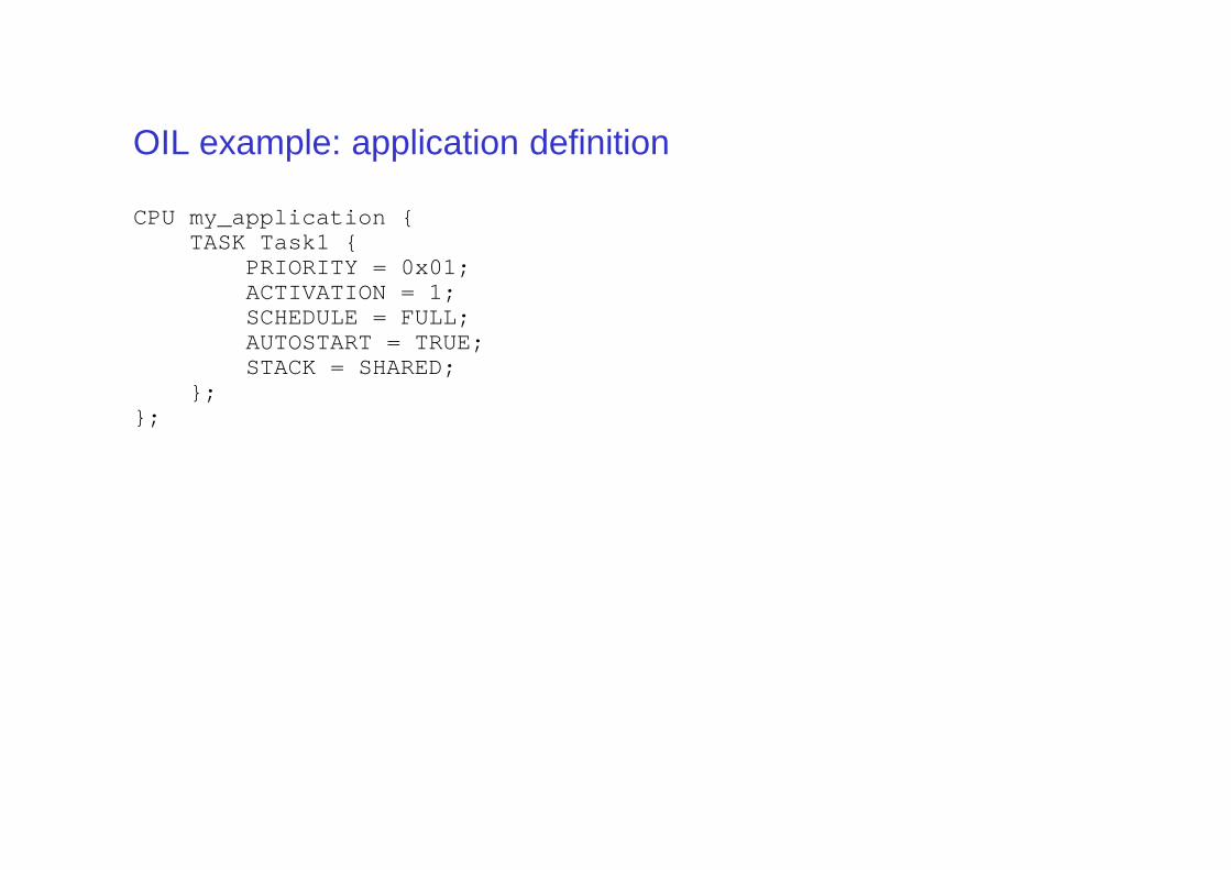
OIL example: application definition
CPU my_application {TASK Task1 {
PRIORITY = 0x01;ACTIVATION = 1;SCHEDULE = FULL;AUTOSTART = TRUE;STACK = SHARED;
};};

That’s all folks !
• Please ask your questions ...
• Backup slides 1- Anomalies and cyclic schedulers
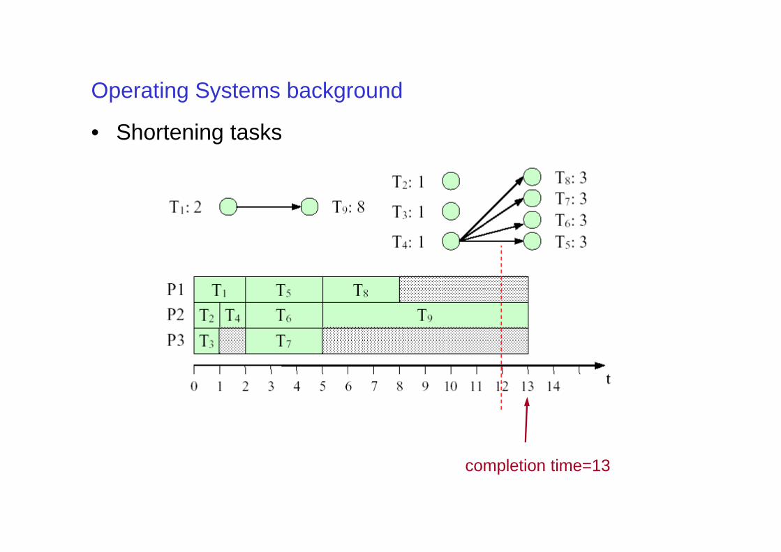
Operating Systems background
• Shortening tasks
completion time=13
Operating Systems background
• Releasing precedence constraints
completion time=16
Background on Operating Systems
Process
• The fundamental concept in any operating system is the “process”
– A process is an executing program
– An OS can execute many processes at the same time (concurrency)
– Example: running a Text Editor and a Web Browser at the same time in the PCtime in the PC
• Processes have separate memory spaces– Each process is assigned a private memory space– One process is not allowed to read or write in the memory space
of another process– If a process tries to access a memory location not in its space,
an exception is raised (Segmentation fault), and the process is terminated
– Two processes cannot directly share variables
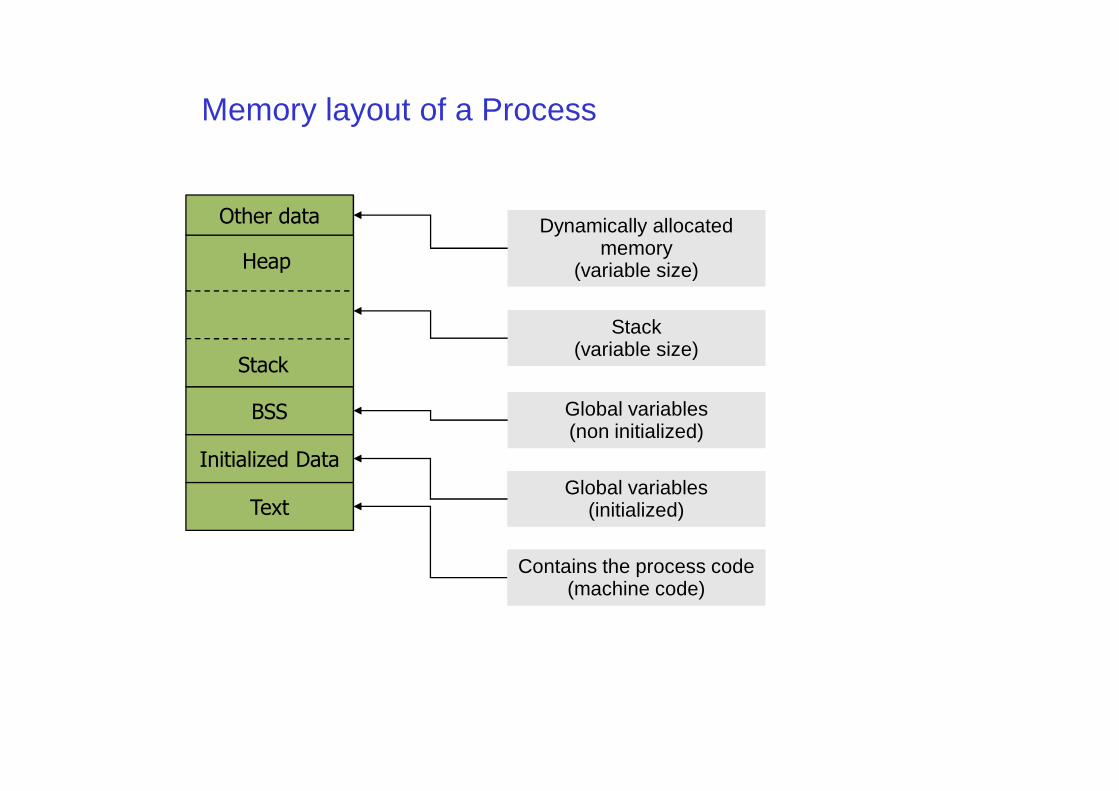
Memory layout of a Process
Stack
Heap
Other data
Stack(variable size)
Stack(variable size)
Dynamically allocatedmemory
(variable size)
Dynamically allocatedmemory
(variable size)
Text
Initialized Data
BSS
Contains the process code(machine code)
Contains the process code(machine code)
Global variables(initialized)
Global variables(initialized)
Global variables(non initialized)Global variables(non initialized)
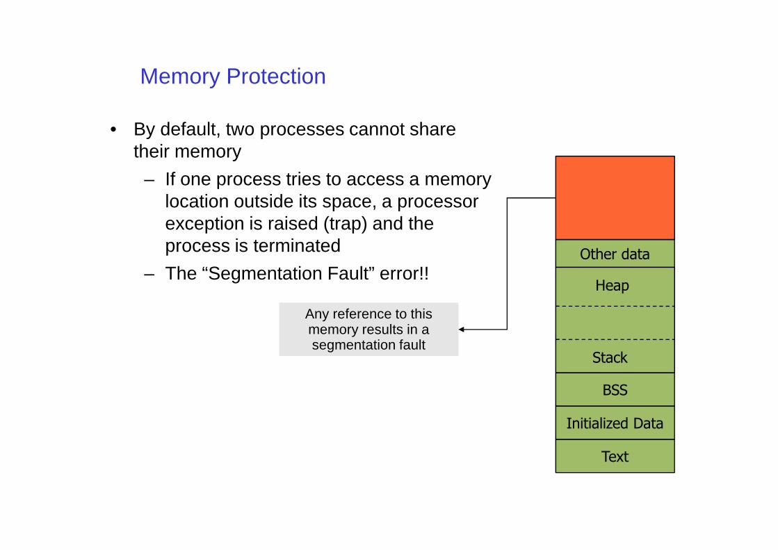
Memory Protection
• By default, two processes cannot share their memory
– If one process tries to access a memory location outside its space, a processor exception is raised (trap) and the process is terminated
– The “Segmentation Fault” error!!Other data
– The “Segmentation Fault” error!!
Text
Initialized Data
BSS
Stack
Heap
Any reference to this memory results in a segmentation fault
Any reference to this memory results in a segmentation fault
Processes
• We can distinguish two aspects in a process
• Resource Ownership– A process includes a virtual address space, a process image
(code + data)
– It is allocated a set of resources, like file descriptors, I/O channels, etc
• Scheduling/Execution• Scheduling/Execution– The execution of a process follows an ececution path, and
generates a trace (sequence of internal states)
– It has a state (ready, Running, etc.)
– And scheduling parameters (priority, time left in the round, etc.)
Multi-threading
• Many OS separate these aspects, by providing the concept of thread
• The process is the “resource owner”
• The thread is the “scheduling entity”– One process can consists of one or more threads
– Threads are sometime called (improperly) lightweight – Threads are sometime called (improperly) lightweight processes
– Therefore, on process can have many different (and concurrent) traces of execution!
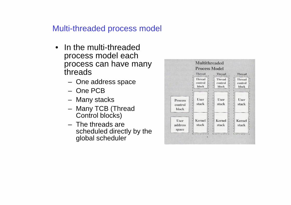
Multi-threaded process model
• In the multi-threaded process model each process can have many threads
– One address space– One PCB– Many stacks– Many stacks– Many TCB (Thread
Control blocks)– The threads are
scheduled directly by the global scheduler
Threads
• Generally, processes do not share memory– To communicate between process, it is necessary to user
OS primitives
– Process switch is more complex because we have to change address space
• Two threads in the same process share the same • Two threads in the same process share the same address space
– They can access the same variables in memory
– Communication between threads is simpler
– Thread switch has less overhead
Threads support in OS
• Different OS implement threads in different ways– Some OS supports directly only processes
• Threads are implemented as “special processes”
– Some OS supports only threads• Processes are threads’ groups
– Some OS natively supports both concepts• For example Windows NT• For example Windows NT
• In Real-Time Operating Systems– Depending on the size and type of system we can have
both threads and processes or only threads– For efficiency reasons, most RTOS only support
• 1 process• Many threads inside the process• All threads share the same memory
– Examples are RTAI, RT-Linux, Shark, some version of VxWorks, QNX, etc.
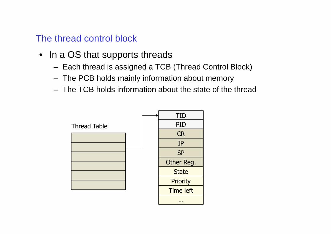
The thread control block
• In a OS that supports threads– Each thread is assigned a TCB (Thread Control Block)– The PCB holds mainly information about memory– The TCB holds information about the state of the thread
TIDTID
PID
CR
IP
SP
Other Reg.
State
Priority
Time left
...
Thread Table
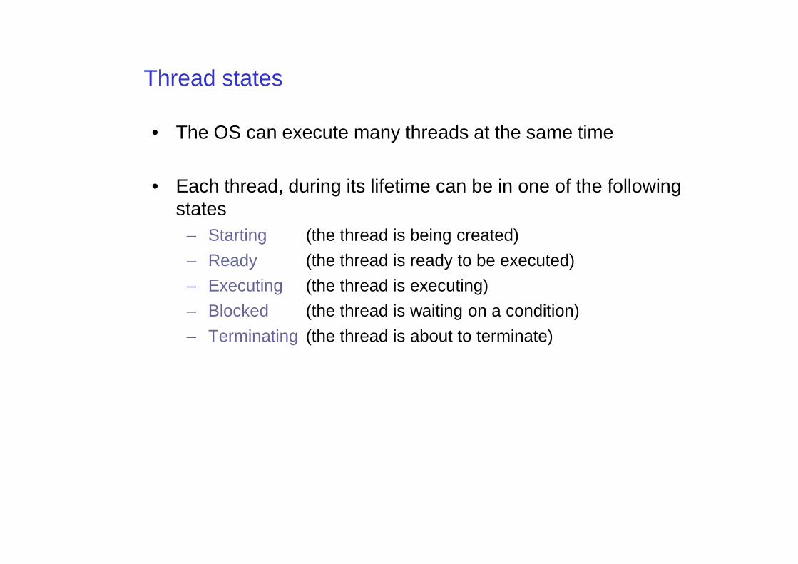
Thread states
• The OS can execute many threads at the same time
• Each thread, during its lifetime can be in one of the following states
– Starting (the thread is being created)
– Ready (the thread is ready to be executed)
– Executing (the thread is executing)– Executing (the thread is executing)
– Blocked (the thread is waiting on a condition)
– Terminating (the thread is about to terminate)
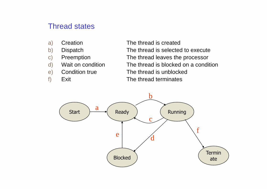
Thread states
a) Creation The thread is createdb) Dispatch The thread is selected to executec) Preemption The thread leaves the processord) Wait on condition The thread is blocked on a conditione) Condition true The thread is unblockedf) Exit The thread terminates
b
Start Ready Running
TerminateBlocked
a
b
c
de f
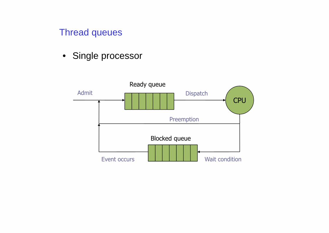
Thread queues
• Single processor
CPU
Ready queue
Admit
Preemption
Dispatch
Preemption
Blocked queue
Wait conditionEvent occurs
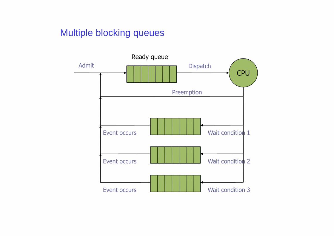
Multiple blocking queues
CPU
Ready queue
Admit
Preemption
Dispatch
Wait condition 1Event occurs
Wait condition 2Event occurs
Wait condition 3Event occurs
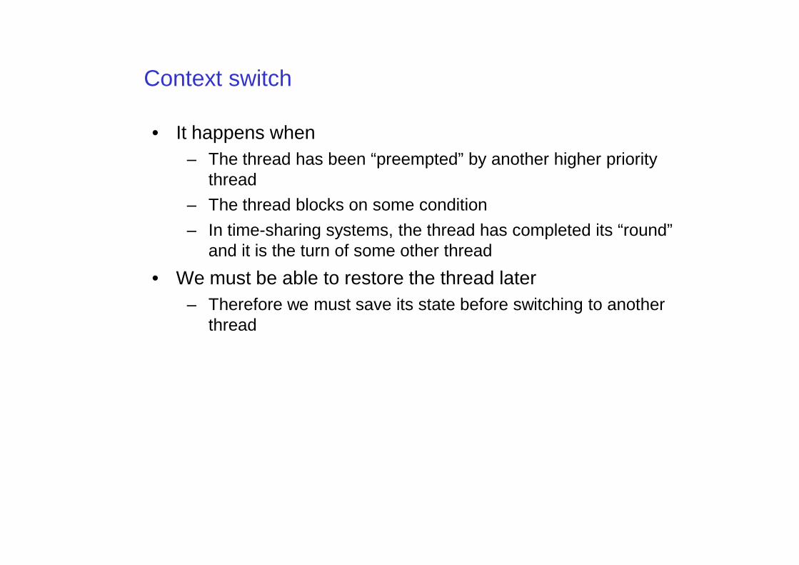
Context switch
• It happens when– The thread has been “preempted” by another higher priority
thread
– The thread blocks on some condition
– In time-sharing systems, the thread has completed its “round” and it is the turn of some other thread
• We must be able to restore the thread later• We must be able to restore the thread later– Therefore we must save its state before switching to another
thread
Context switch
• This is only an example– Every OS has little variations on the same theme
– For example, in most cases, registers are saved on the stack, not on the TCB
• You can try to look into some real OS– Linux– Linux
– Free BSD
– Shark (http://shark.sssup.it)
– Every OS is different!
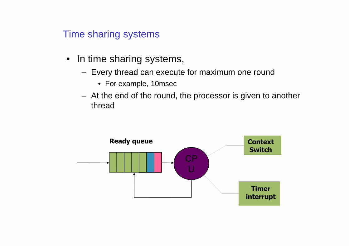
Time sharing systems
• In time sharing systems, – Every thread can execute for maximum one round
• For example, 10msec
– At the end of the round, the processor is given to another thread
Context
Switch
CPU
Ready queue
CPU
CPU
CPU
Timer
interrupt
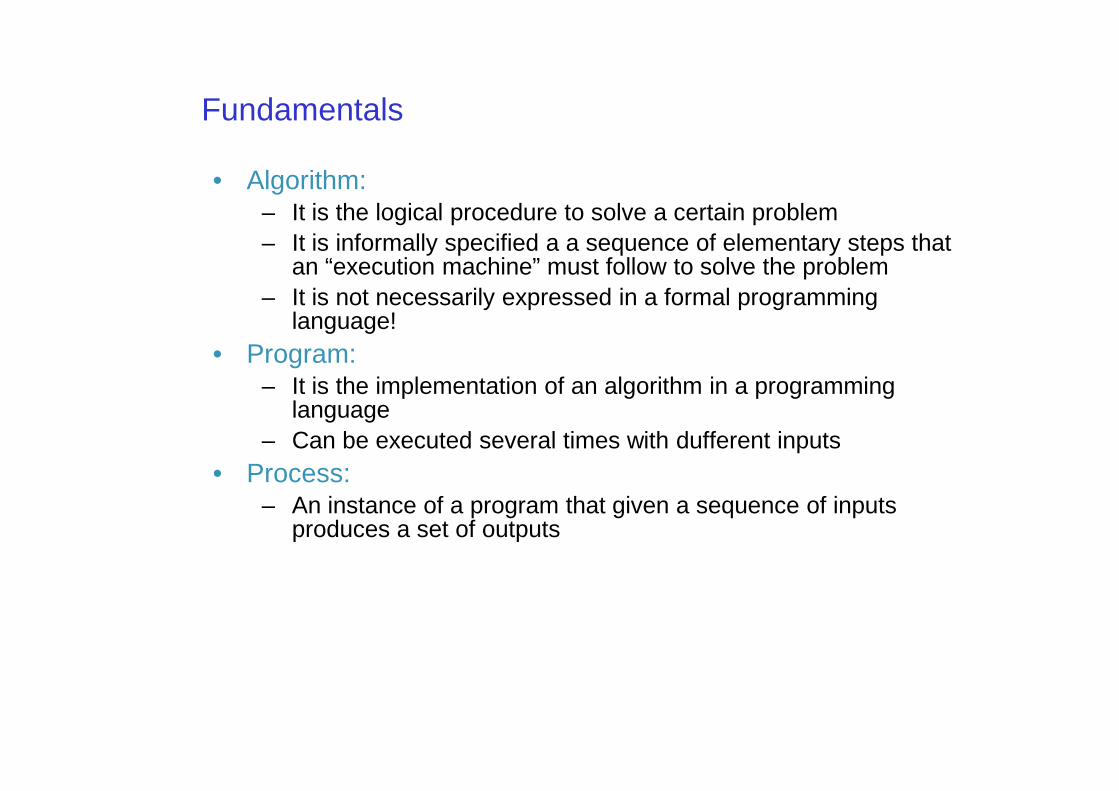
Fundamentals
• Algorithm:– It is the logical procedure to solve a certain problem– It is informally specified a a sequence of elementary steps that
an “execution machine” must follow to solve the problem– It is not necessarily expressed in a formal programming
language!• Program:
– It is the implementation of an algorithm in a programming – It is the implementation of an algorithm in a programming language
– Can be executed several times with dufferent inputs• Process:
– An instance of a program that given a sequence of inputs produces a set of outputs
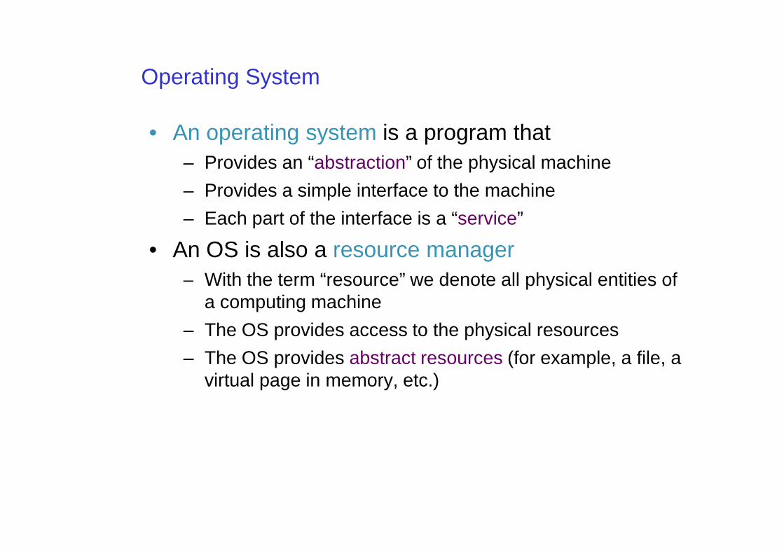
Operating System
• An operating system is a program that– Provides an “abstraction” of the physical machine
– Provides a simple interface to the machine
– Each part of the interface is a “service”
• An OS is also a resource manager– With the term “resource” we denote all physical entities of – With the term “resource” we denote all physical entities of
a computing machine
– The OS provides access to the physical resources
– The OS provides abstract resources (for example, a file, a virtual page in memory, etc.)
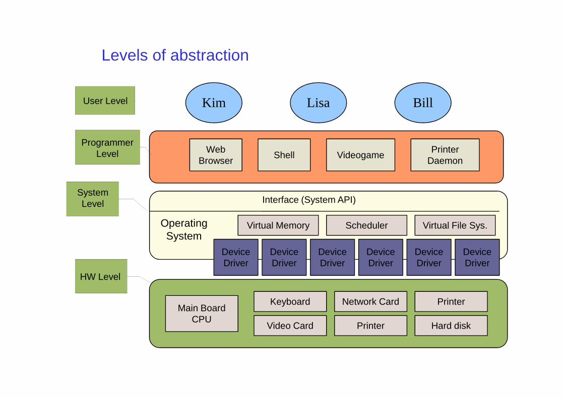
Levels of abstraction
Kim Lisa Bill
Interface (System API)
Web Browser
Shell VideogamePrinter
Daemon
User Level
ProgrammerLevel
SystemLevel
Main Board CPU
Keyboard
Video Card
Network Card
Printer
Printer
Hard disk
OperatingSystem
Interface (System API)
Virtual Memory Scheduler Virtual File Sys.
Device Driver
Device Driver
Device Driver
Device Driver
Device Driver
Device Driver
Level
HW Level
Abstraction mechanisms
• Why abstraction?– Programming the HW directly has several drawbacks
• It is difficult and error-prone
• It is not portable
– Suppose you want to write a program that reads a text file from disk and outputs it on the screen
• Without a proper interface it is virtually impossible!
Abstraction Mechanisms
• Application programming interface (API)– Provides a convenient and uniform way to access to one
service so that• HW details are hidden to the high level programmer
• One application does not depend on the HW
• The programmer can concentrate on higher level tasks
– Example– Example• For reading a file, linux and many other unix OS provide the
open(), read() system calls that, given a “file name” allow to load the data from an external support
Classification of OS - II• By objective
– General purpouse (windows, linux, etc), – Servers,– RTOS
• By size– Full featured– Embedded OS– Nano-kernels– Nano-kernels
• By internal structure– Monolithic– Micro-kernel
the need for concurrency
• there are many reason for concurrency– functional– performance– expressive power
• functional– many users may be connected to the same system at the – many users may be connected to the same system at the
same time• each user can have its own processes that execute
concurrently with the processes of the other users
– perform many operations concurrently• for example, listen to music, write with a word processor, burn a
CD, etc...• they are all different and independent activities• they can be done “at the same time”
the need for concurrency (2)
• performance– take advantage of blocking time
• while some thread waits for a blocking condition, another thread performs another operation
– parallelism in multi-processor machines• if we have a multi-processor machine, independent activities can be
carried out on different processors are the same time
• expressive power• expressive power– many control application are inherently concurrent– concurrency support helps in expressing concurrency, making
application development simpler
theoretical model
• a system is a set of concurrent activities– they can be processes or threads
• they interact in two ways– they access the hardware resources
• processor• disk• memory, etc.• memory, etc.
– they exchange data
• these activities compete for the resources and/or cooperate for some common objective
resource
• a resource can be– a HW resource like a I/O device– a SW resource, i.e. a data structure– in both cases, access to a resource must be regulated to
avoid interference
• example 1– if two processes want to print on the same printer, their – if two processes want to print on the same printer, their
access must be sequentialised, otherwise the two printing could be intermangled!
• example 2– if two threads access the same data structure, the operation
on the data must be sequentialized otherwise the data could be inconsistent!
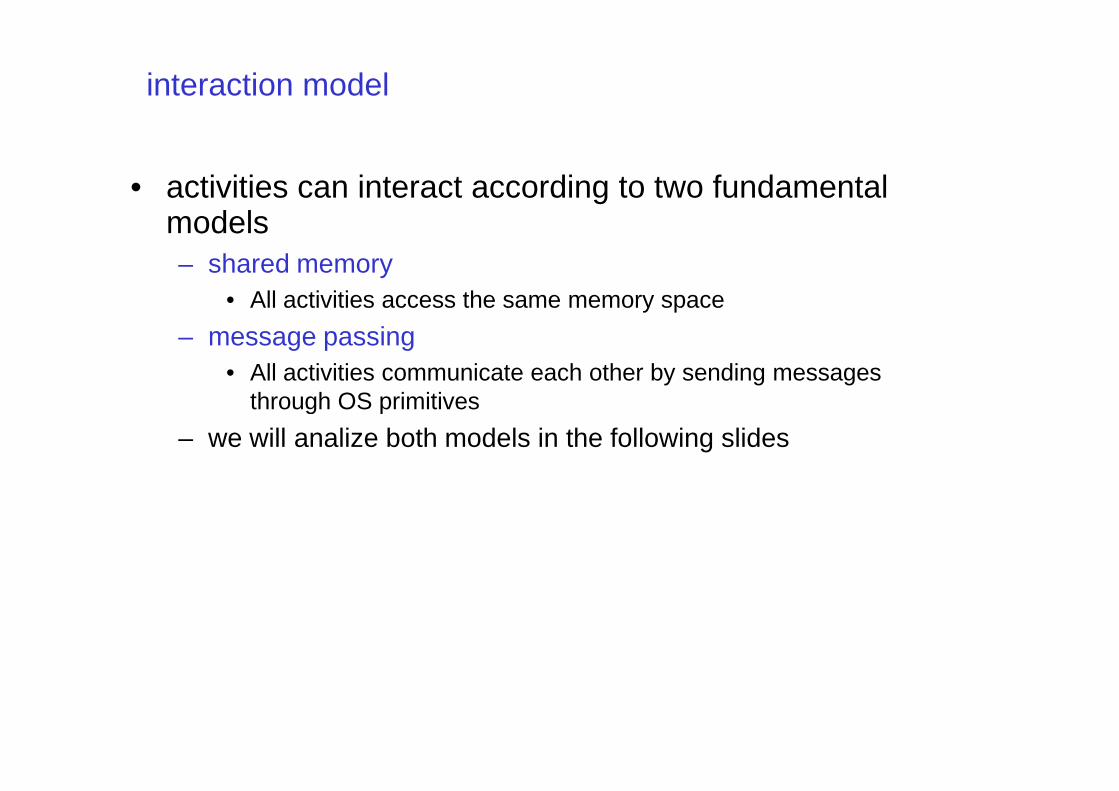
interaction model
• activities can interact according to two fundamental models– shared memory
• All activities access the same memory space
– message passing• All activities communicate each other by sending messages
through OS primitivesthrough OS primitives
– we will analize both models in the following slides
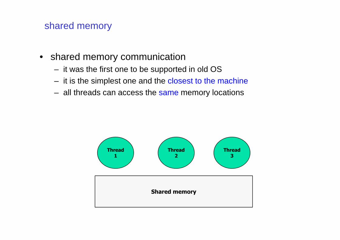
shared memory
• shared memory communication– it was the first one to be supported in old OS– it is the simplest one and the closest to the machine– all threads can access the same memory locations
Thread 1
Thread 2
Thread 3
Shared memory
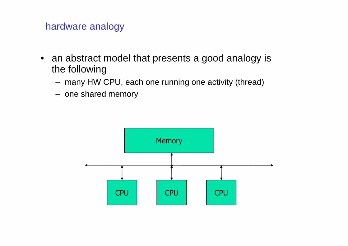
hardware analogy
• an abstract model that presents a good analogy is the following– many HW CPU, each one running one activity (thread)– one shared memory
CPU CPU CPU
Memory
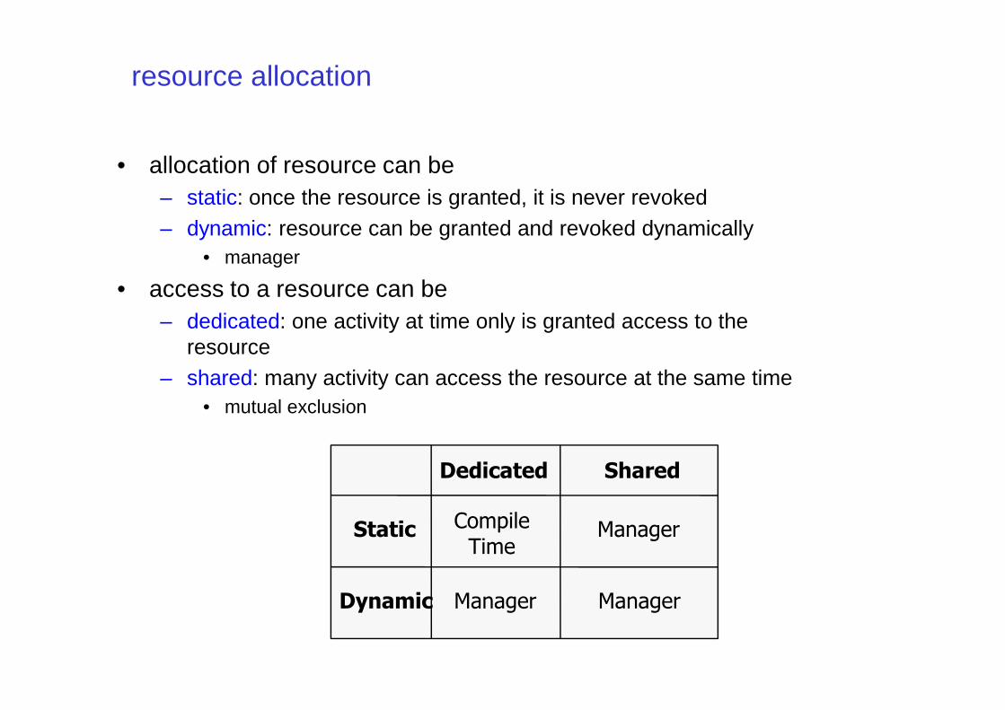
resource allocation
• allocation of resource can be – static: once the resource is granted, it is never revoked– dynamic: resource can be granted and revoked dynamically
• manager
• access to a resource can be– dedicated: one activity at time only is granted access to the
resourceresource– shared: many activity can access the resource at the same time
• mutual exclusion
Dedicated Shared
Static
Dynamic
CompileTime
Manager
ManagerManager
mutual exclusion problem
• we do not know in advance the relative speed of the processes– hence, we do not know the order of execution of the
hardware instructions
• recall the example of incrementing variable x– incrementing x is not an atomic operation– atomic behavior can be obtained using interrupt disabling or
special atomic instructions
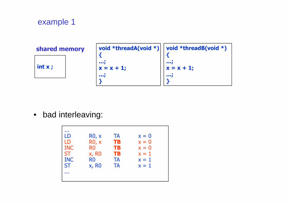
example 1
int x ;
shared memory void *threadA(void *)
{
...;
x = x + 1;
...;
}
void *threadB(void *)
{
...;
x = x + 1;
...;
}
• bad interleaving:
...LD R0, x TA x = 0LD R0, x TB x = 0INC R0 TB x = 0ST x, R0 TB x = 1INC R0 TA x = 1ST x, R0 TA x = 1...
critical sections
• definitions– the shared object where the conflict may happen is a “resource”– the parts of the code where the problem may happen are called
“critical sections”• a critical section is a sequence of operations that cannot be interleaved
with other operations on the same resource
– two critical sections on the same resource must be properly sequentializedsequentialized
– we say that two critical sections on the same resource must execute in MUTUAL EXCLUSION
– there are three ways to obtain motual exclusion• implementing the critical section as an atomic operation• disabling the preemption (system-wide)• selectively disabling the preemption (using semaphores and mutual
exclusion)
critical sections: atomic operations
• in single processor systems– disable interrupts during a critical section
• problems:– if the critical section is long, no interrupt can arrive during the
critical section• consider a timer interrupt that arrives every 1 msec. • if a critical section lasts for more than 1 msec, a timer interrupt • if a critical section lasts for more than 1 msec, a timer interrupt
could be lost!– concurrency is disabled during the critical section!
• we must avoid conflicts on the resource, not disabling interrupts!
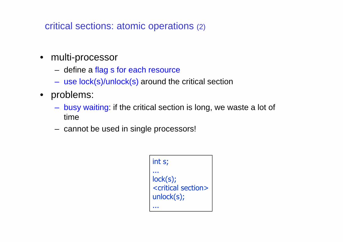
critical sections: atomic operations (2)
• multi-processor– define a flag s for each resource– use lock(s)/unlock(s) around the critical section
• problems:– busy waiting: if the critical section is long, we waste a lot of
timetime– cannot be used in single processors!
int s;...lock(s);<critical section>unlock(s);...
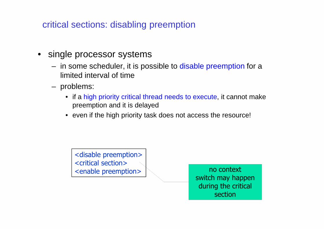
critical sections: disabling preemption
• single processor systems– in some scheduler, it is possible to disable preemption for a
limited interval of time– problems:
• if a high priority critical thread needs to execute, it cannot make preemption and it is delayed
• even if the high priority task does not access the resource!• even if the high priority task does not access the resource!
<disable preemption><critical section><enable preemption> no context
switch may happen during the critical
section
general mechanism: semaphores
• Djikstra proposed the semaphore mechanism– a semaphore is an abstract entity that consists
• a counter• a blocking queue• operation wait• operation signal
– the operations on a semaphore are considered atomic– the operations on a semaphore are considered atomic
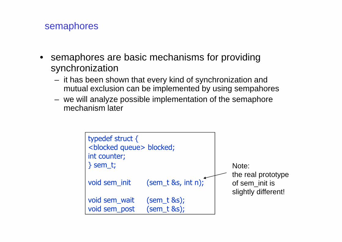
semaphores
• semaphores are basic mechanisms for providing synchronization– it has been shown that every kind of synchronization and
mutual exclusion can be implemented by using sempahores– we will analyze possible implementation of the semaphore
mechanism later
typedef struct {<blocked queue> blocked;int counter;} sem_t;
void sem_init (sem_t &s, int n);
void sem_wait (sem_t &s);void sem_post (sem_t &s);
Note:the real prototype of sem_init is slightly different!
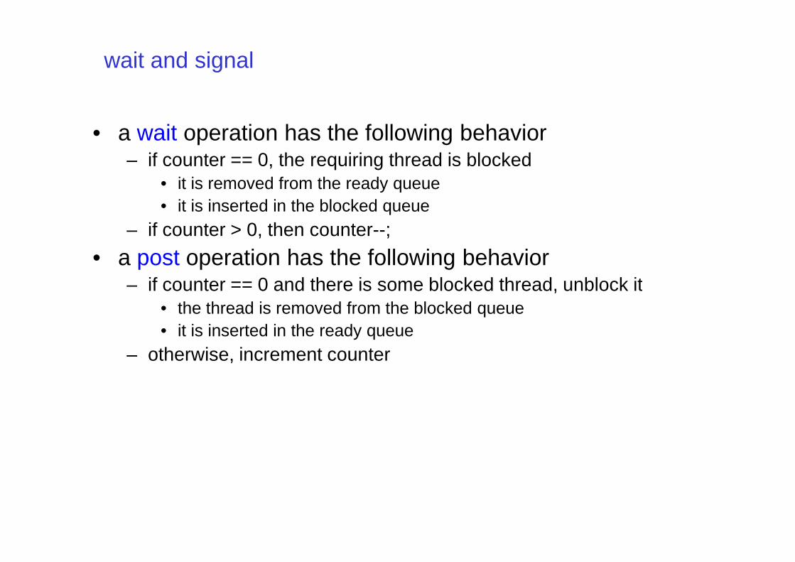
wait and signal
• a wait operation has the following behavior– if counter == 0, the requiring thread is blocked
• it is removed from the ready queue• it is inserted in the blocked queue
– if counter > 0, then counter--;
• a post operation has the following behavior– if counter == 0 and there is some blocked thread, unblock it– if counter == 0 and there is some blocked thread, unblock it
• the thread is removed from the blocked queue• it is inserted in the ready queue
– otherwise, increment counter
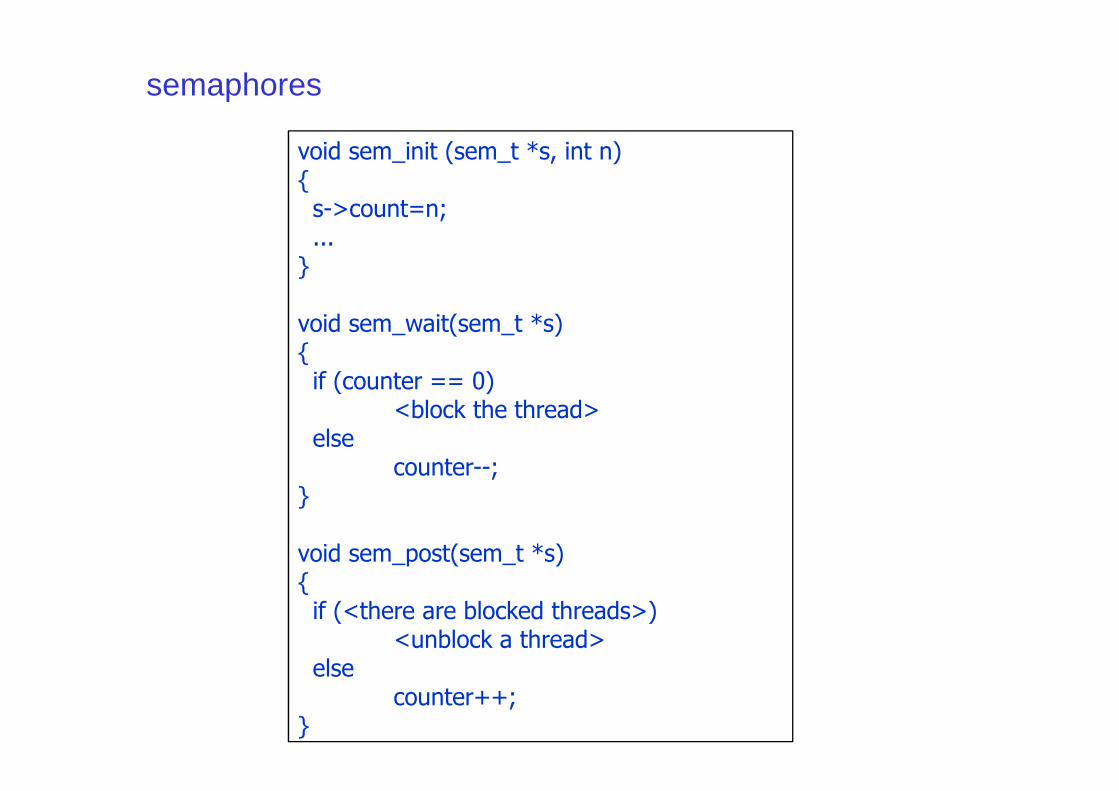
semaphores
void sem_init (sem_t *s, int n) {s->count=n;...
}
void sem_wait(sem_t *s) {if (counter == 0)
<block the thread><block the thread>else
counter--;}
void sem_post(sem_t *s) {if (<there are blocked threads>)
<unblock a thread>else
counter++; }
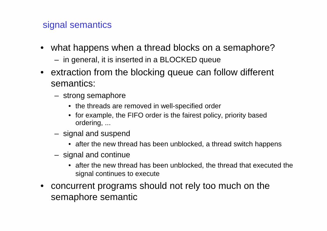
signal semantics
• what happens when a thread blocks on a semaphore?– in general, it is inserted in a BLOCKED queue
• extraction from the blocking queue can follow different semantics:– strong semaphore
• the threads are removed in well-specified order • for example, the FIFO order is the fairest policy, priority based • for example, the FIFO order is the fairest policy, priority based
ordering, ...
– signal and suspend• after the new thread has been unblocked, a thread switch happens
– signal and continue• after the new thread has been unblocked, the thread that executed the
signal continues to execute
• concurrent programs should not rely too much on the semaphore semantic
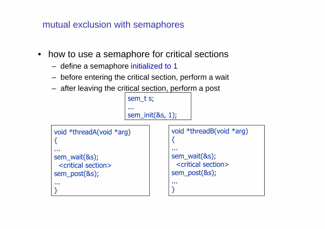
mutual exclusion with semaphores
• how to use a semaphore for critical sections– define a semaphore initialized to 1– before entering the critical section, perform a wait– after leaving the critical section, perform a post
sem_t s;...sem_init(&s, 1);sem_init(&s, 1);
void *threadA(void *arg){...sem_wait(&s);<critical section>
sem_post(&s);...}
void *threadB(void *arg){...sem_wait(&s);<critical section>
sem_post(&s);...}
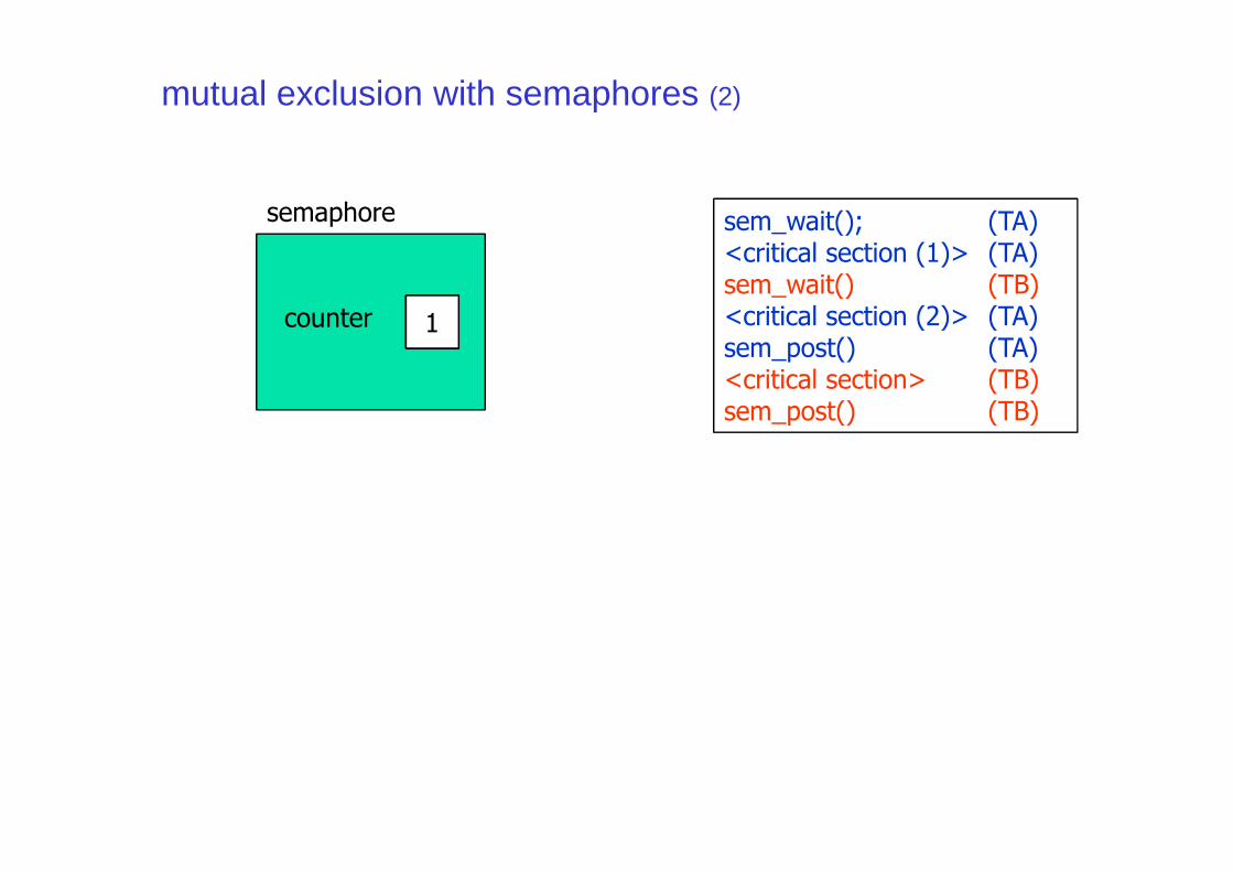
mutual exclusion with semaphores (2)
semaphore
counter 10
sem_wait(); (TA)<critical section (1)> (TA)sem_wait() (TB)<critical section (2)> (TA)sem_post() (TA)<critical section> (TB)sem_post() (TB)
1
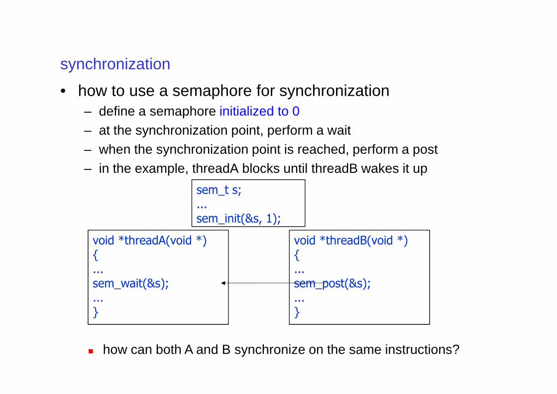
synchronization
• how to use a semaphore for synchronization– define a semaphore initialized to 0– at the synchronization point, perform a wait– when the synchronization point is reached, perform a post– in the example, threadA blocks until threadB wakes it up
sem_t s;...
void *threadA(void *){...sem_wait(&s);...}
void *threadB(void *){...sem_post(&s);...}
� how can both A and B synchronize on the same instructions?
...sem_init(&s, 1);
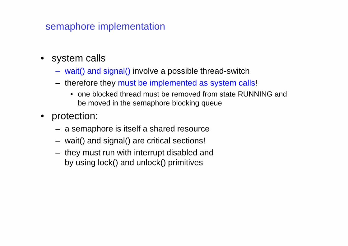
semaphore implementation
• system calls– wait() and signal() involve a possible thread-switch– therefore they must be implemented as system calls!
• one blocked thread must be removed from state RUNNING and be moved in the semaphore blocking queue
• protection:– a semaphore is itself a shared resource– wait() and signal() are critical sections!– they must run with interrupt disabled and
by using lock() and unlock() primitives
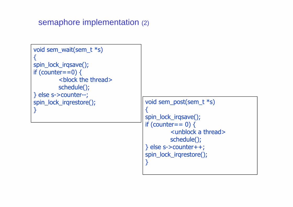
semaphore implementation (2)
void sem_wait(sem_t *s){spin_lock_irqsave();if (counter==0) {
<block the thread>schedule();
} else s->counter--;spin_lock_irqrestore(); void sem_post(sem_t *s)spin_lock_irqrestore();}
void sem_post(sem_t *s){spin_lock_irqsave();if (counter== 0) {
<unblock a thread>schedule();
} else s->counter++;spin_lock_irqrestore();}
monitors
• monitors are a language structure equivalent to semaphores, but cleaner– a monitor is similar to an object in a OO language– it contains variables and provides procedures to other
software modules– only one thread can execute a procedure at a certain time
• any other thread that has invoked the procedure is blocked and • any other thread that has invoked the procedure is blocked and waits for the first threads to exit
• therefore, a monitor implicitely provides mutual exclusion
– the source code that is used to implement the mutual exclusion is automatically inserted by the compiler
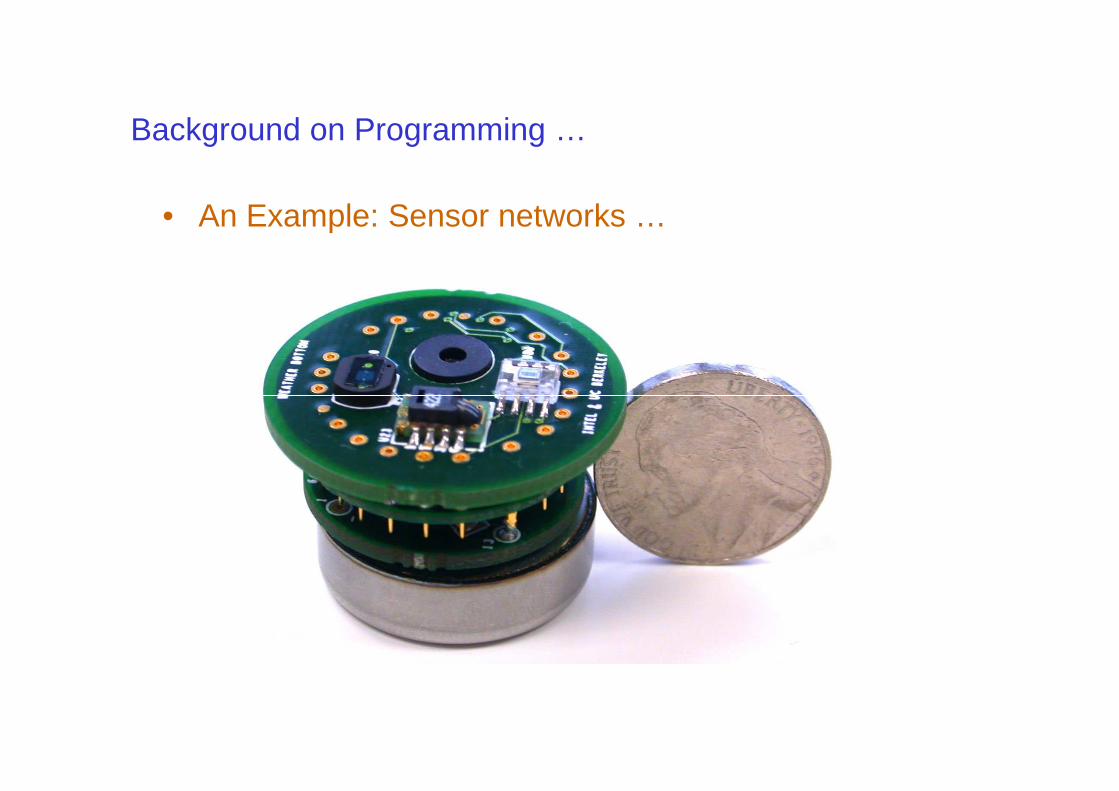
Background on Programming …
• An Example: Sensor networks …
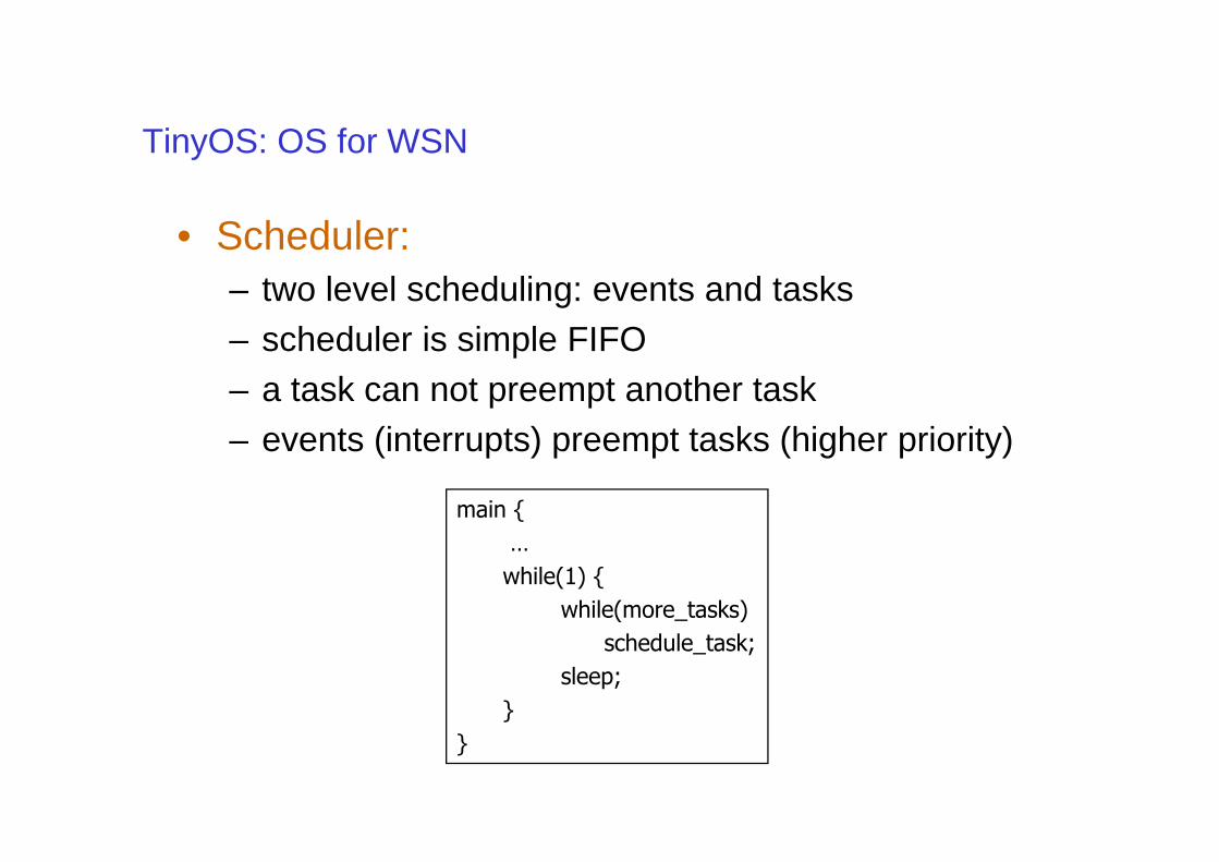
TinyOS: OS for WSN
• Scheduler:– two level scheduling: events and tasks– scheduler is simple FIFO– a task can not preempt another task– events (interrupts) preempt tasks (higher priority)– events (interrupts) preempt tasks (higher priority)
main {
…
while(1) {
while(more_tasks)
schedule_task;
sleep;
}
}
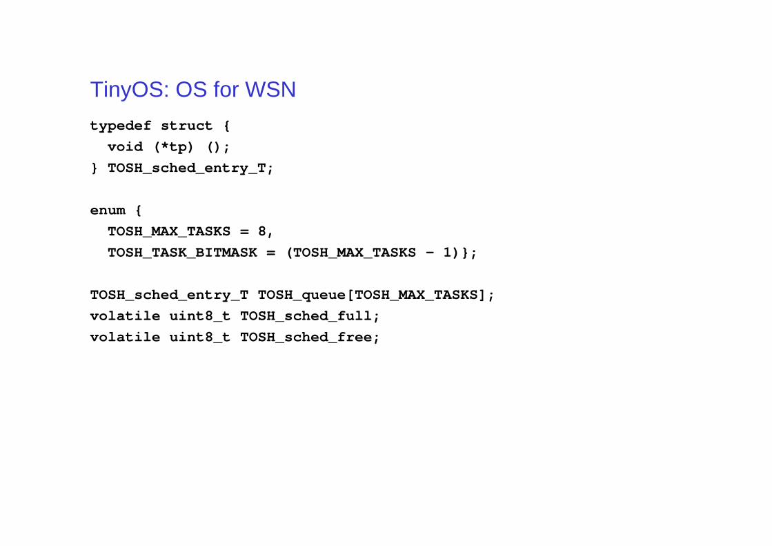
TinyOS: OS for WSN
typedef struct {
void (*tp) ();
} TOSH_sched_entry_T;
enum {
TOSH_MAX_TASKS = 8,
TOSH_TASK_BITMASK = (TOSH_MAX_TASKS - 1)};
TOSH_sched_entry_T TOSH_queue[TOSH_MAX_TASKS];
volatile uint8_t TOSH_sched_full;
volatile uint8_t TOSH_sched_free;
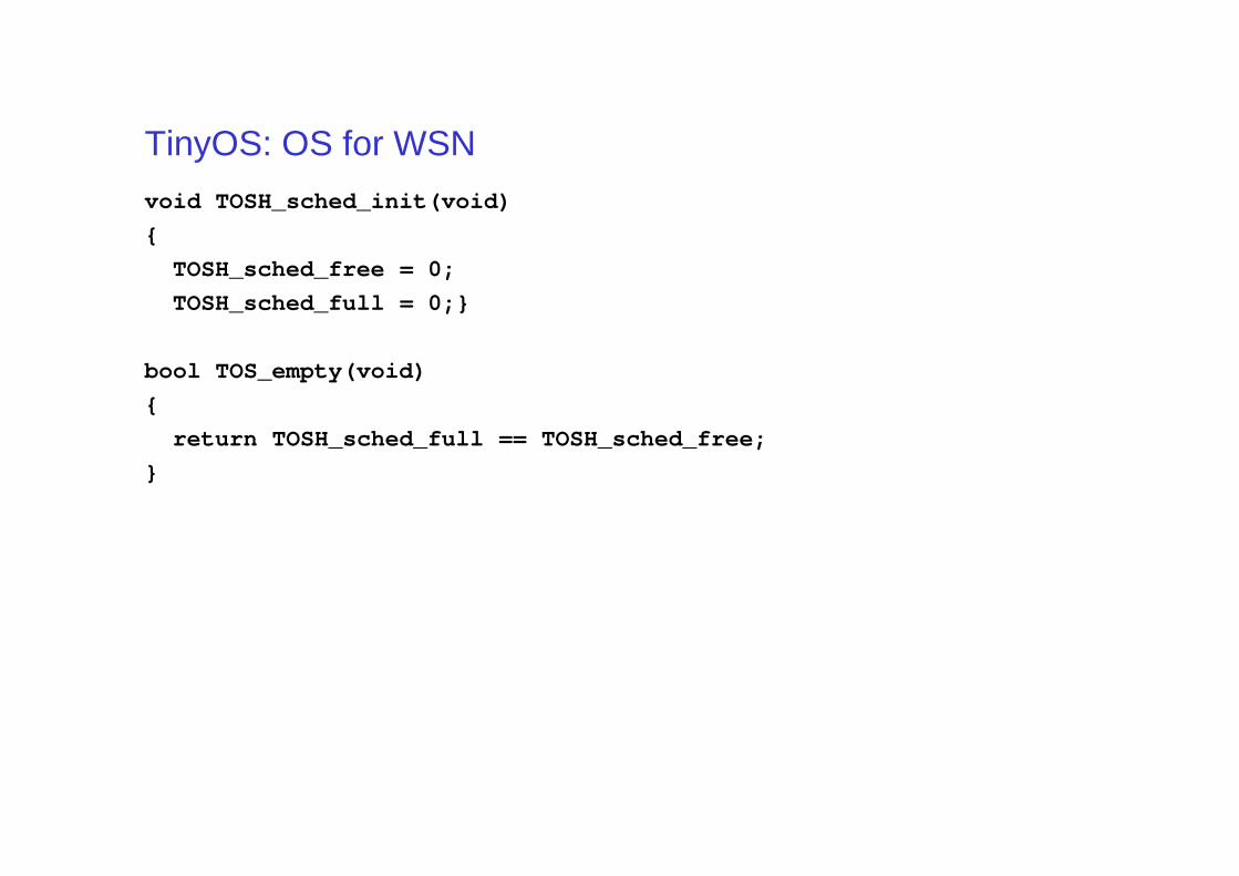
TinyOS: OS for WSN
void TOSH_sched_init(void)
{
TOSH_sched_free = 0;
TOSH_sched_full = 0;}
bool TOS_empty(void)
{
return TOSH_sched_full == TOSH_sched_free;return TOSH_sched_full == TOSH_sched_free;
}
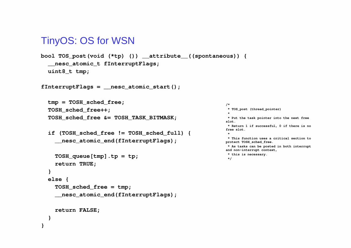
TinyOS: OS for WSNbool TOS_post(void (*tp) ()) __attribute__((spontaneous)) {
__nesc_atomic_t fInterruptFlags;
uint8_t tmp;
fInterruptFlags = __nesc_atomic_start();
tmp = TOSH_sched_free;
TOSH_sched_free++;
TOSH_sched_free &= TOSH_TASK_BITMASK;
/** TOS_post (thread_pointer)* * Put the task pointer into the next free slot.
if (TOSH_sched_free != TOSH_sched_full) {
__nesc_atomic_end(fInterruptFlags);
TOSH_queue[tmp].tp = tp;
return TRUE;
}
else {
TOSH_sched_free = tmp;
__nesc_atomic_end(fInterruptFlags);
return FALSE;
}
}
* Return 1 if successful, 0 if there is no free slot.** This function uses a critical section to protect TOSH_sched_free.* As tasks can be posted in both interrupt and non-interrupt context,* this is necessary.*/
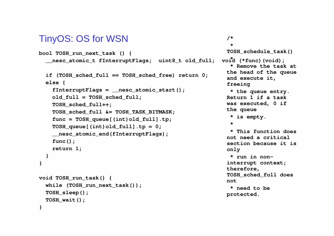
TinyOS: OS for WSNbool TOSH_run_next_task () {
__nesc_atomic_t fInterruptFlags; uint8_t old_full; void (*func)(void);
if (TOSH_sched_full == TOSH_sched_free) return 0;
else {
fInterruptFlags = __nesc_atomic_start();
old_full = TOSH_sched_full;
TOSH_sched_full++;
TOSH_sched_full &= TOSH_TASK_BITMASK;
func = TOSH_queue[(int)old_full].tp;
/*
* TOSH_schedule_task()
*
* Remove the task at the head of the queue and execute it, freeing
* the queue entry. Return 1 if a task was executed, 0 if the queue
* is empty.func = TOSH_queue[(int)old_full].tp;
TOSH_queue[(int)old_full].tp = 0;
__nesc_atomic_end(fInterruptFlags);
func();
return 1;
}
}
void TOSH_run_task() {
while (TOSH_run_next_task());
TOSH_sleep();
TOSH_wait();
}
* is empty.
*
* This function does not need a critical section because it is only
* run in non-interrupt context; therefore, TOSH_sched_full does not
* need to be protected.
• Processor demand criterion
Response Time Analysis
• Response time Analysis runs in pseudopolynomial time
• Is it possible to know a-priori the time intervals over which the test should be performed?– The iterative procedure tests against increasing intervals
corresponding to the wikcorresponding to the wi
• The alternative method is called processor demand criterion
• It applies to the case of static and dynamic priority
Fixed Priority Scheduling
• Utilization-based Analysis• Response time Analysis• Processor Demand Analysis
– Important: allows for sensitivity analysis ....
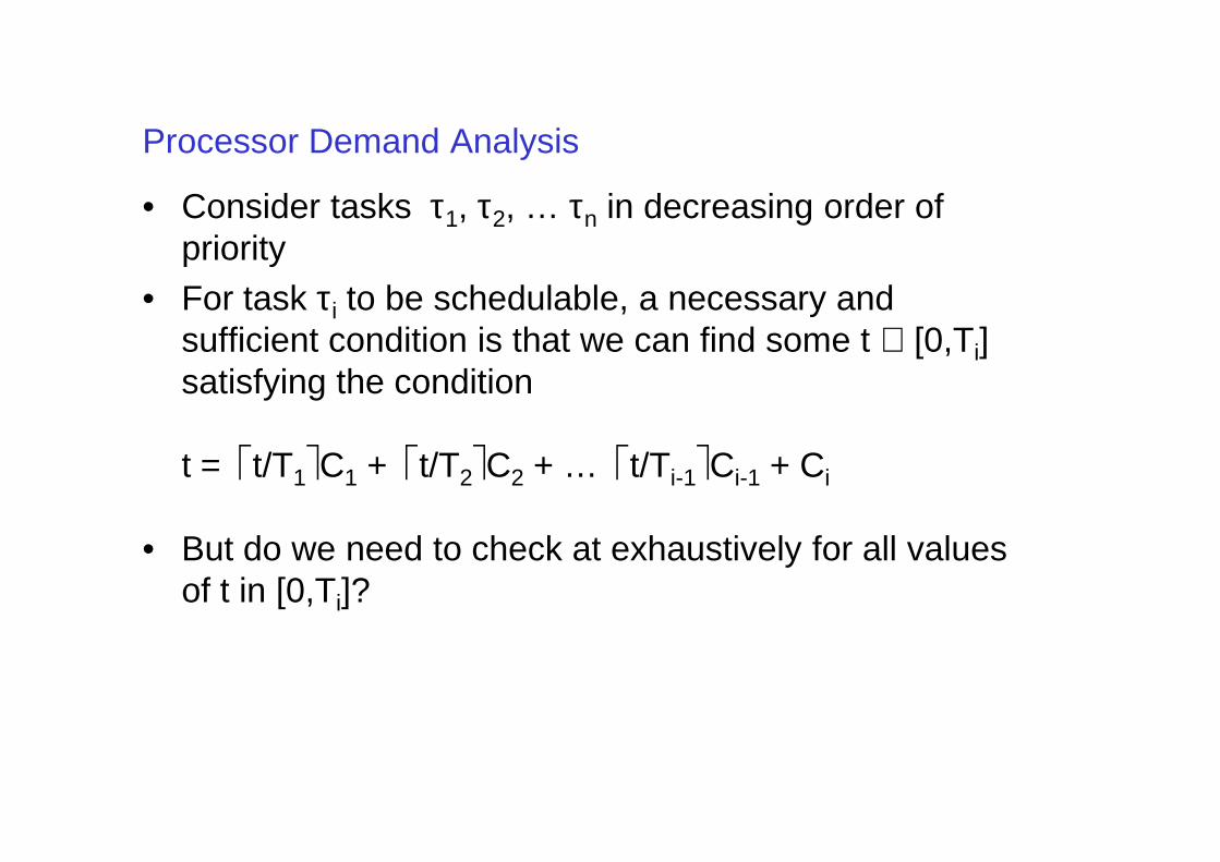
Processor Demand Analysis
• Consider tasks τ1, τ2, … τn in decreasing order of priority
• For task τi to be schedulable, a necessary and sufficient condition is that we can find some t ∈ [0,Ti] satisfying the condition
t = t/T1C1 + t/T2C2 + … t/Ti-1Ci-1 + Ci
• But do we need to check at exhaustively for all values of t in [0,Ti]?
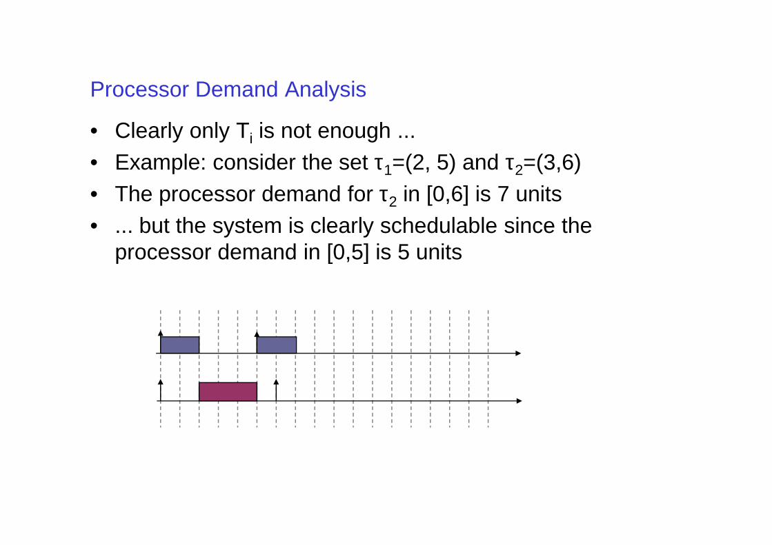
Processor Demand Analysis
• Clearly only Ti is not enough ... • Example: consider the set τ1=(2, 5) and τ2=(3,6)• The processor demand for τ2 in [0,6] is 7 units• ... but the system is clearly schedulable since the
processor demand in [0,5] is 5 units
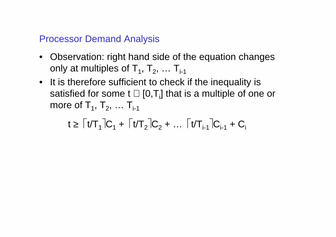
Processor Demand Analysis
• Observation: right hand side of the equation changes only at multiples of T1, T2, … Ti-1
• It is therefore sufficient to check if the inequality is satisfied for some t ∈ [0,Ti] that is a multiple of one or more of T1, T2, … Ti-1
≥ t ≥ t/T1C1 + t/T2C2 + … t/Ti-1Ci-1 + Ci
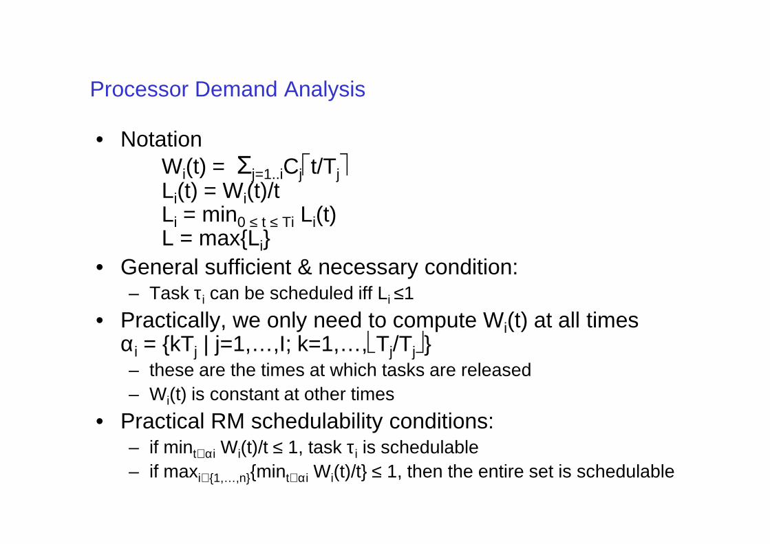
Processor Demand Analysis
• NotationWi(t) = Σj=1..iCjt/TjLi(t) = Wi(t)/tLi = min0 ≤ t ≤ Ti Li(t)L = max{Li}
• General sufficient & necessary condition:• General sufficient & necessary condition:– Task τi can be scheduled iff Li ≤1
• Practically, we only need to compute Wi(t) at all timesαi = {kTj | j=1,…,I; k=1,…,Tj/Tj}– these are the times at which tasks are released– Wi(t) is constant at other times
• Practical RM schedulability conditions:– if mint∈αi Wi(t)/t ≤ 1, task τi is schedulable– if maxi∈{1,…,n}{mint∈αi Wi(t)/t} ≤ 1, then the entire set is schedulable
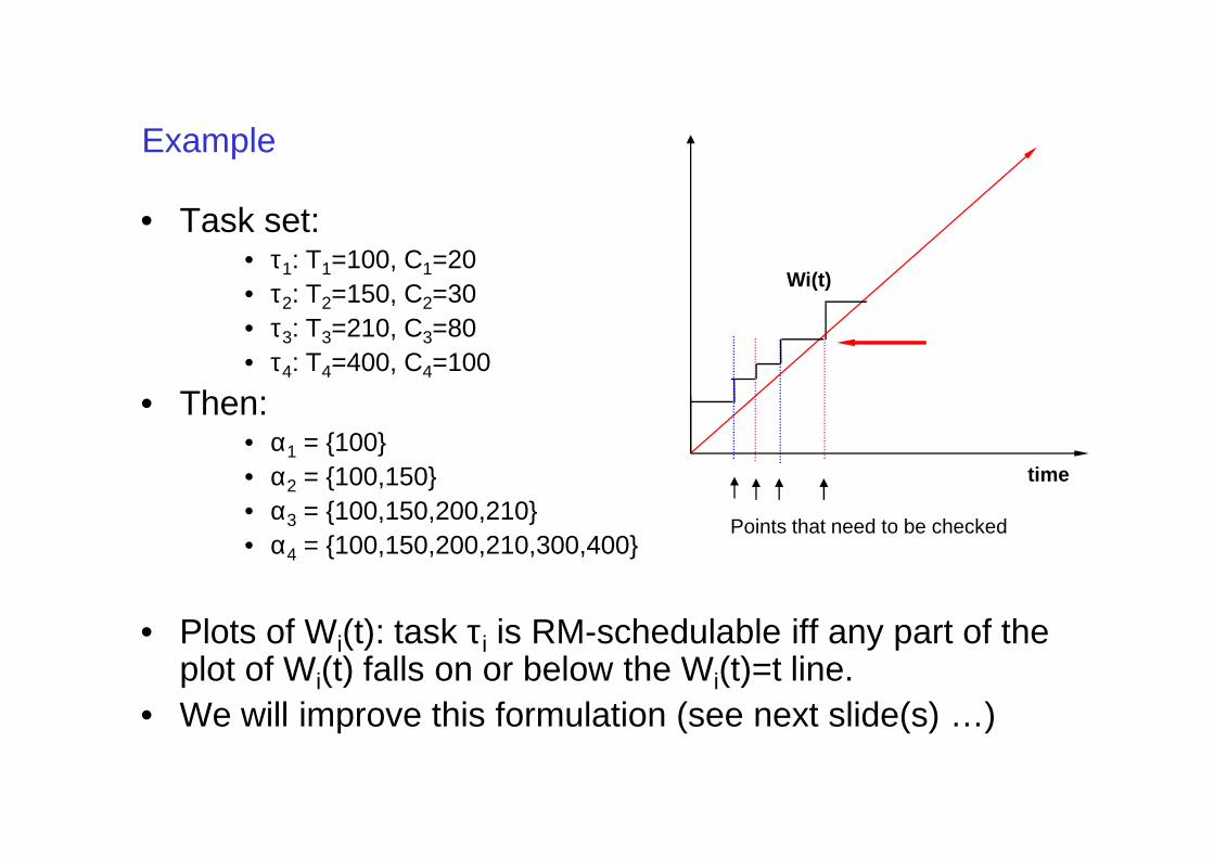
Example
• Task set:• τ1: T1=100, C1=20• τ2: T2=150, C2=30• τ3: T3=210, C3=80• τ4: T4=400, C4=100
• Then:• α = {100}
Wi(t)
• α1 = {100}• α2 = {100,150}• α3 = {100,150,200,210}• α4 = {100,150,200,210,300,400}
• Plots of Wi(t): task τi is RM-schedulable iff any part of the plot of Wi(t) falls on or below the Wi(t)=t line.
• We will improve this formulation (see next slide(s) …)
time
Points that need to be checked
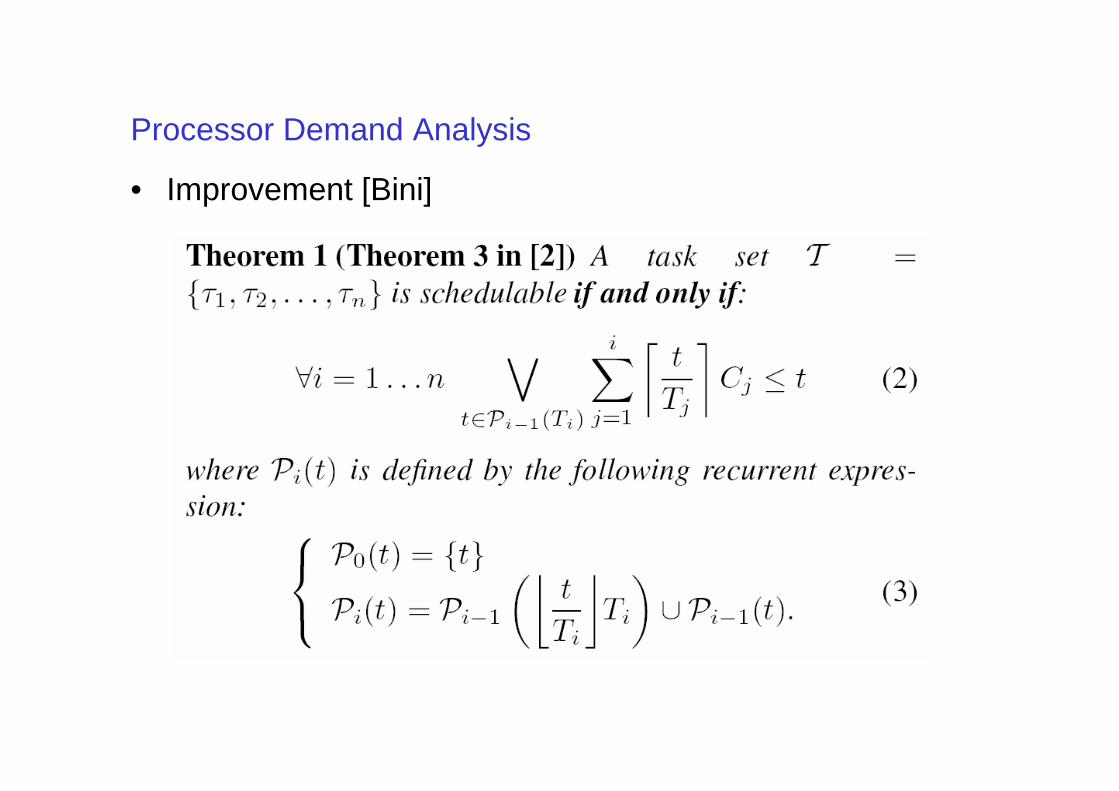
Processor Demand Analysis
• Improvement [Bini]
• Backup Scaife-Caspi
An introduction to Real-Time scheduling
• Asynchronous interactions (Scaife & Caspi [Euromicro2004], figures from the paper)
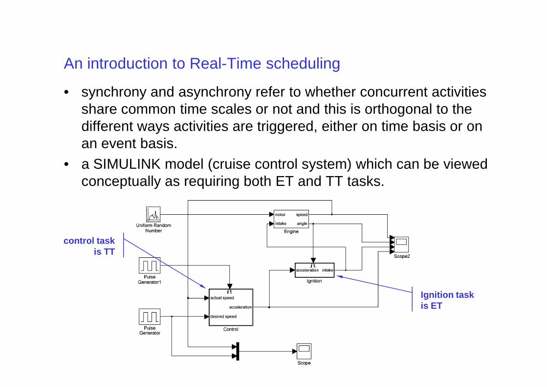
An introduction to Real-Time scheduling
• synchrony and asynchrony refer to whether concurrent activities share common time scales or not and this is orthogonal to the different ways activities are triggered, either on time basis or on an event basis.
• a SIMULINK model (cruise control system) which can be viewed conceptually as requiring both ET and TT tasks.
control task is TT
Ignition task is ET
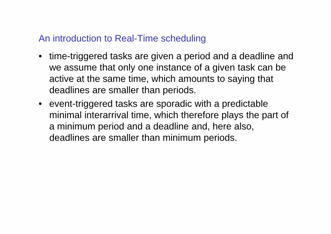
An introduction to Real-Time scheduling
• time-triggered tasks are given a period and a deadline and we assume that only one instance of a given task can be active at the same time, which amounts to saying that deadlines are smaller than periods.
• event-triggered tasks are sporadic with a predictable minimal interarrival time, which therefore plays the part of minimal interarrival time, which therefore plays the part of a minimum period and a deadline and, here also, deadlines are smaller than minimum periods.
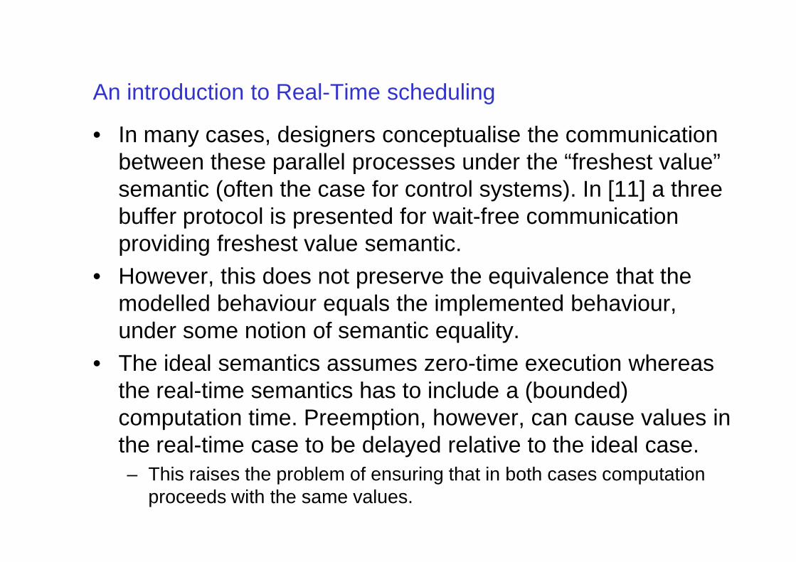
An introduction to Real-Time scheduling
• In many cases, designers conceptualise the communication between these parallel processes under the “freshest value” semantic (often the case for control systems). In [11] a three buffer protocol is presented for wait-free communication providing freshest value semantic.
• However, this does not preserve the equivalence that the • However, this does not preserve the equivalence that the modelled behaviour equals the implemented behaviour, under some notion of semantic equality.
• The ideal semantics assumes zero-time execution whereas the real-time semantics has to include a (bounded) computation time. Preemption, however, can cause values in the real-time case to be delayed relative to the ideal case.– This raises the problem of ensuring that in both cases computation
proceeds with the same values.
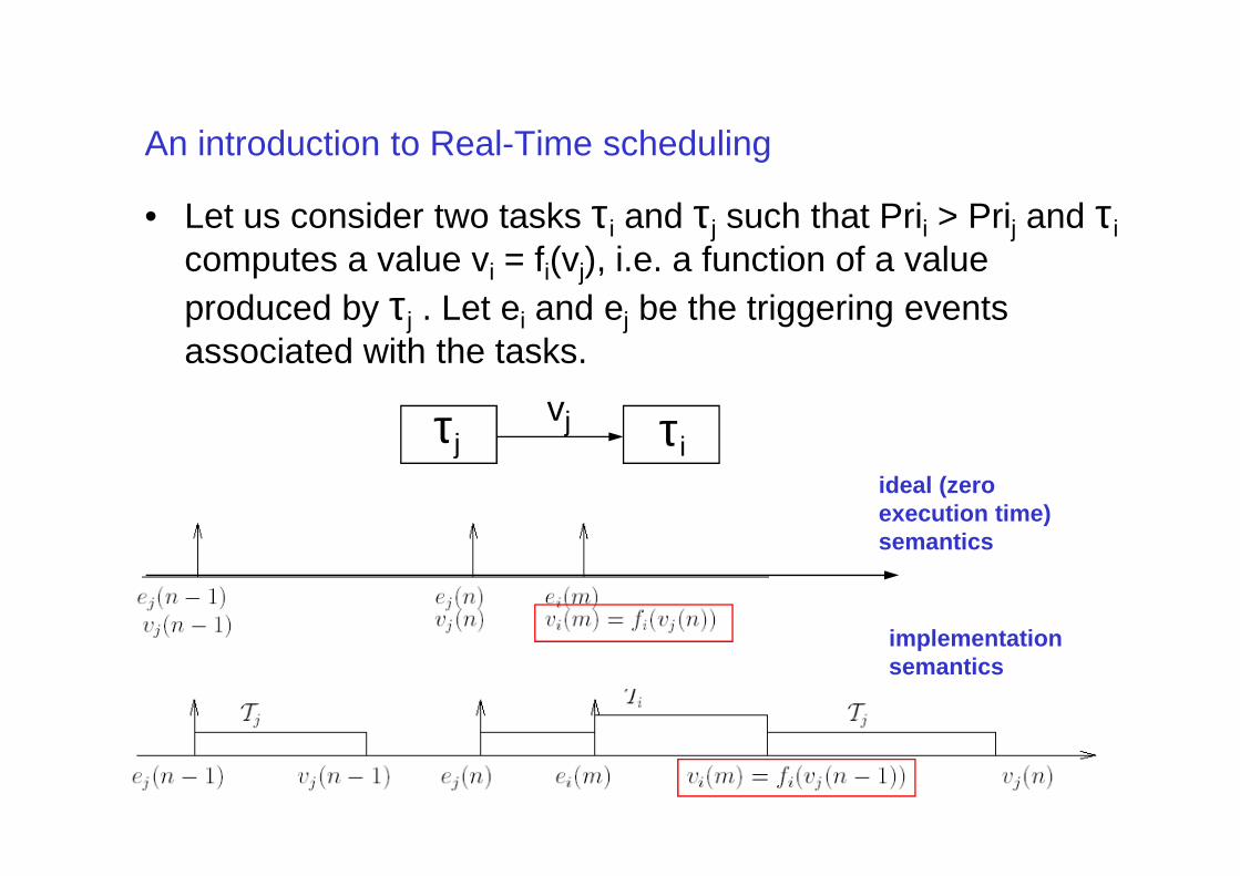
An introduction to Real-Time scheduling
• Let us consider two tasks τi and τj such that Prii > Prij and τi
computes a value vi = fi(vj), i.e. a function of a value produced by τj . Let ei and ej be the triggering events associated with the tasks.
τiτjvj τiτj
ideal (zero execution time) semantics
implementation semantics
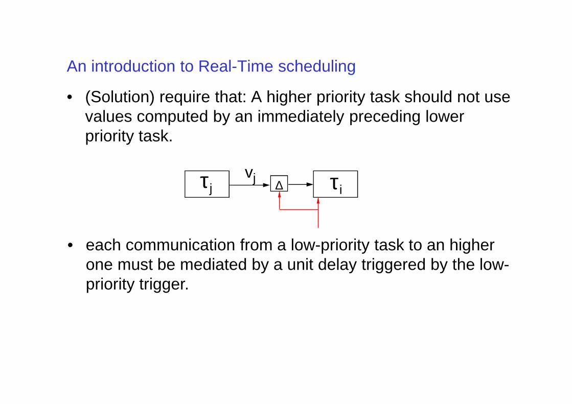
An introduction to Real-Time scheduling
• (Solution) require that: A higher priority task should not use values computed by an immediately preceding lower priority task.
τiτjvj ∆
• each communication from a low-priority task to an higher one must be mediated by a unit delay triggered by the low-priority trigger.
An introduction to Real-Time scheduling
• In a communication from high to low, it may be the case that the low-priority task starts reading, but is interrupted by the high-priority task which changes its results. When the lower priority task resumes reading, it will get incoherent data.
• Even when communications are buffered as in the case of • Even when communications are buffered as in the case of low to high communications, undesirable effects can take place
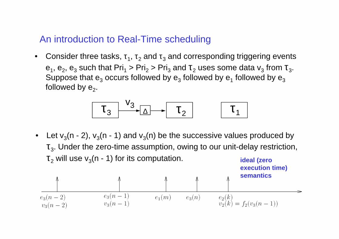
An introduction to Real-Time scheduling
• Consider three tasks, τ1, τ2 and τ3 and corresponding triggering events e1, e2, e3 such that Pri1 > Pri2 > Pri3 and τ2 uses some data v3 from τ3. Suppose that e3 occurs followed by e3 followed by e1 followed by e3followed by e2.
τ2τ3v3 τ1∆
• Let v3(n - 2), v3(n - 1) and v3(n) be the successive values produced by τ3. Under the zero-time assumption, owing to our unit-delay restriction, τ2 will use v3(n - 1) for its computation. ideal (zero
execution time) semantics
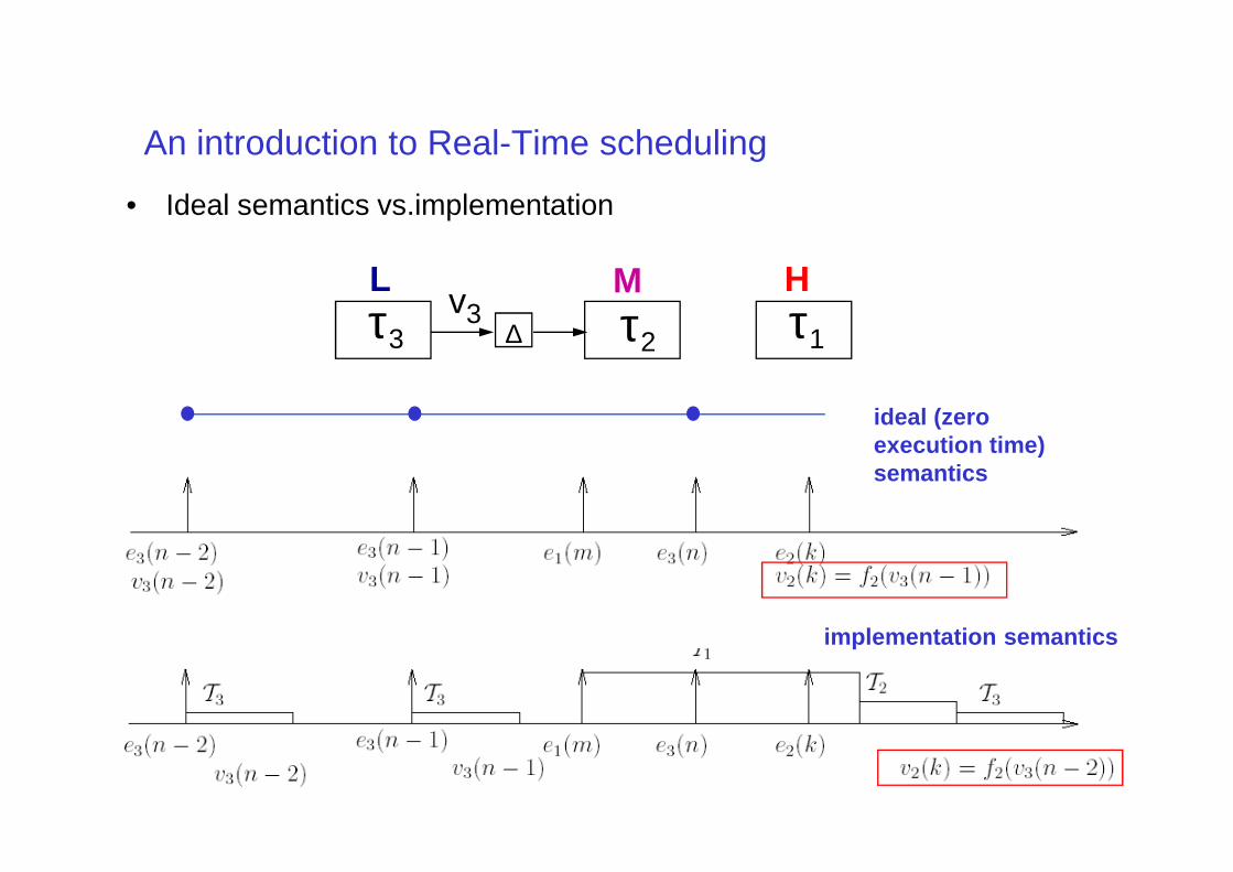
An introduction to Real-Time scheduling
• Ideal semantics vs.implementation
τ2τ3v3 τ1
ideal (zero execution time)
HML∆
execution time) semantics
implementation semantics
An introduction to Real-Time scheduling
• if we want to keep in the implementation the same order of communication as in the model, the buffering mechanism should be controlled by the triggering event occurrences and not by the task executions.
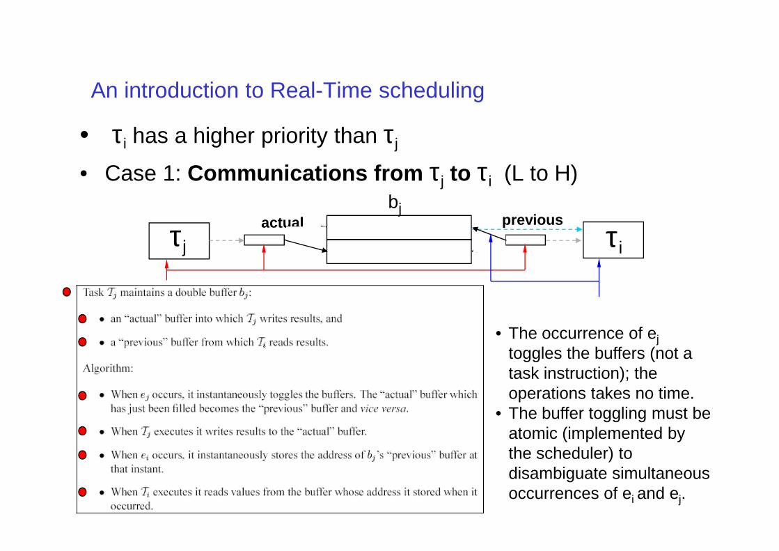
An introduction to Real-Time scheduling
• τi has a higher priority than τj
• Case 1: Communications from τj to τi (L to H)
previous
τiτjactual
bj
• The occurrence of ejtoggles the buffers (not a task instruction); the operations takes no time.
• The buffer toggling must be atomic (implemented by the scheduler) to disambiguate simultaneous occurrences of ei and ej.
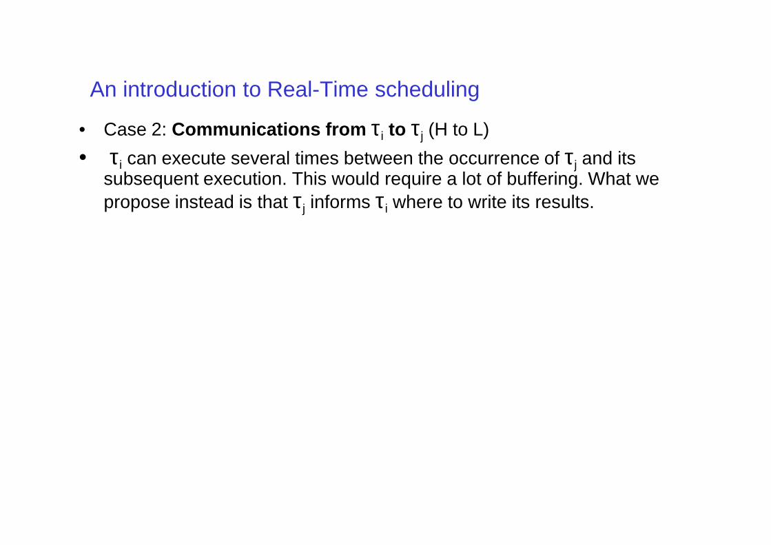
An introduction to Real-Time scheduling
• Case 2: Communications from τi to τj (H to L)
• τi can execute several times between the occurrence of τj and its subsequent execution. This would require a lot of buffering. What we propose instead is that τj informs τi where to write its results.
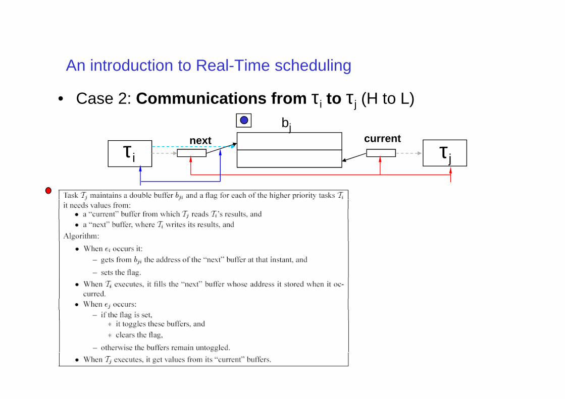
An introduction to Real-Time scheduling
• Case 2: Communications from τi to τj (H to L)
current
τjτinext
bj
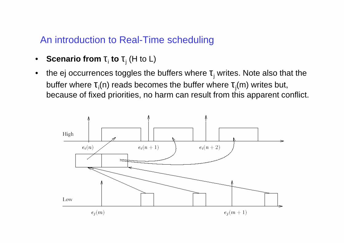
An introduction to Real-Time scheduling
• Scenario from τi to τj (H to L)
• the ej occurrences toggles the buffers where τj writes. Note also that the buffer where τi(n) reads becomes the buffer where τj(m) writes but, because of fixed priorities, no harm can result from this apparent conflict.
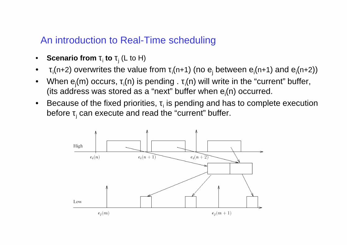
An introduction to Real-Time scheduling
• Scenario from τi to τj (L to H)
• τi(n+2) overwrites the value from τi(n+1) (no ej between ei(n+1) and ei(n+2))• When ej(m) occurs, τi(n) is pending . τi(n) will write in the “current” buffer,
(its address was stored as a “next” buffer when ei(n) occurred. • Because of the fixed priorities, τi is pending and has to complete execution
before τj can execute and read the “current” buffer.
Recommended