An Introduction to Hawkes Processeswith Applications to Finance
Ioane Muni Toke
Ecole Centrale ParisBNP Paribas Chair of Quantitative Finance
February 4th, 2011
Ioane Muni Toke (ECP - BNPP Chair) An Introduction to Hawkes Processes February 4th, 2011 1 / 90
Table of contents
1 An Introduction to Point Processes
2 One-dimensional Hawkes processes
3 Multidimensional Hawkes processes
4 A simple model for buy and sell intensities
5 Modelling microstructure noise
6 Some statistical findings about the order book
7 An order book model with Hawkes processes
Ioane Muni Toke (ECP - BNPP Chair) An Introduction to Hawkes Processes February 4th, 2011 2 / 90
An Introduction to Point Processes
Table of contents
1 An Introduction to Point ProcessesBasic definitionsTransformation to Poisson processes
2 One-dimensional Hawkes processesDefinition and stationarity propertiesSimulation of a Hawkes processMaximum-likelihood estimation
3 Multidimensional Hawkes processesDefinition and stationarity conditionSimulation of a multivariate Hawkes processMaximum-likelihood estimation
4 A simple model for buy and sell intensities
5 Modelling microstructure noise
6 Some statistical findings about the order book
7 An order book model with Hawkes processes
Ioane Muni Toke (ECP - BNPP Chair) An Introduction to Hawkes Processes February 4th, 2011 3 / 90
An Introduction to Point Processes Basic definitions
Table of contents
1 An Introduction to Point ProcessesBasic definitionsTransformation to Poisson processes
2 One-dimensional Hawkes processesDefinition and stationarity propertiesSimulation of a Hawkes processMaximum-likelihood estimation
3 Multidimensional Hawkes processesDefinition and stationarity conditionSimulation of a multivariate Hawkes processMaximum-likelihood estimation
4 A simple model for buy and sell intensities
5 Modelling microstructure noise
6 Some statistical findings about the order book
7 An order book model with Hawkes processes
Ioane Muni Toke (ECP - BNPP Chair) An Introduction to Hawkes Processes February 4th, 2011 4 / 90
An Introduction to Point Processes Basic definitions
Simple point processes
Point process
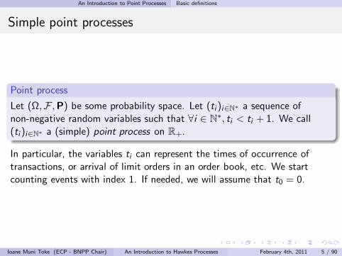
Let (Ω,F ,P) be some probability space. Let (ti )i∈N∗ a sequence ofnon-negative random variables such that ∀i ∈ N
∗, ti < ti + 1. We call(ti )i∈N∗ a (simple) point process on R+.
In particular, the variables ti can represent the times of occurrence oftransactions, or arrival of limit orders in an order book, etc. We startcounting events with index 1. If needed, we will assume that t0 = 0.
Ioane Muni Toke (ECP - BNPP Chair) An Introduction to Hawkes Processes February 4th, 2011 5 / 90
An Introduction to Point Processes Basic definitions
Counting process and durations
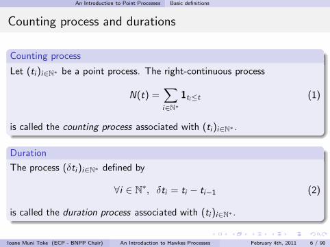
Counting process
Let (ti)i∈N∗ be a point process. The right-continuous process
N(t) =∑
i∈N∗
1ti≤t (1)
is called the counting process associated with (ti)i∈N∗ .
Duration
The process (δti )i∈N∗ defined by
∀i ∈ N∗, δti = ti − ti−1 (2)
is called the duration process associated with (ti )i∈N∗ .
Ioane Muni Toke (ECP - BNPP Chair) An Introduction to Hawkes Processes February 4th, 2011 6 / 90
An Introduction to Point Processes Basic definitions
Representation of a simple point process
0
1
2
3
4
t1 t2 t3 t4Time
δt2
Counting process NEvents t
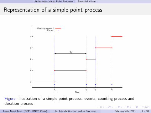
Figure: Illustration of a simple point process: events, counting process andduration process
Ioane Muni Toke (ECP - BNPP Chair) An Introduction to Hawkes Processes February 4th, 2011 7 / 90
An Introduction to Point Processes Basic definitions
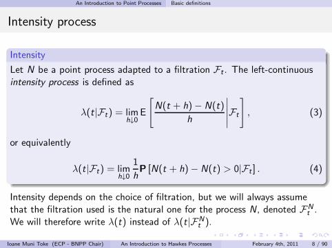
Intensity process
Intensity
Let N be a point process adapted to a filtration Ft . The left-continuousintensity process is defined as
λ(t|Ft) = limh↓0
E
[
N(t + h)− N(t)
h
∣
∣
∣
∣
∣
Ft
]
, (3)
or equivalently
λ(t|Ft) = limh↓0
1
hP [N(t + h)− N(t) > 0|Ft ] . (4)
Intensity depends on the choice of filtration, but we will always assumethat the filtration used is the natural one for the process N, denoted FN
t .We will therefore write λ(t) instead of λ(t|FN
t ).
Ioane Muni Toke (ECP - BNPP Chair) An Introduction to Hawkes Processes February 4th, 2011 8 / 90
An Introduction to Point Processes Basic definitions
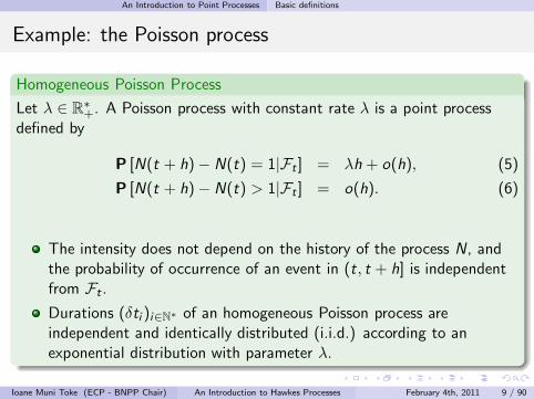
Example: the Poisson process
Homogeneous Poisson Process
Let λ ∈ R∗+. A Poisson process with constant rate λ is a point process
defined by
P [N(t + h)− N(t) = 1|Ft ] = λh + o(h), (5)
P [N(t + h)− N(t) > 1|Ft ] = o(h). (6)
The intensity does not depend on the history of the process N, andthe probability of occurrence of an event in (t, t + h] is independentfrom Ft .
Durations (δti )i∈N∗ of an homogeneous Poisson process areindependent and identically distributed (i.i.d.) according to anexponential distribution with parameter λ.
Ioane Muni Toke (ECP - BNPP Chair) An Introduction to Hawkes Processes February 4th, 2011 9 / 90
An Introduction to Point Processes Transformation to Poisson processes
Table of contents
1 An Introduction to Point ProcessesBasic definitionsTransformation to Poisson processes
2 One-dimensional Hawkes processesDefinition and stationarity propertiesSimulation of a Hawkes processMaximum-likelihood estimation
3 Multidimensional Hawkes processesDefinition and stationarity conditionSimulation of a multivariate Hawkes processMaximum-likelihood estimation
4 A simple model for buy and sell intensities
5 Modelling microstructure noise
6 Some statistical findings about the order book
7 An order book model with Hawkes processes
Ioane Muni Toke (ECP - BNPP Chair) An Introduction to Hawkes Processes February 4th, 2011 10 / 90
An Introduction to Point Processes Transformation to Poisson processes
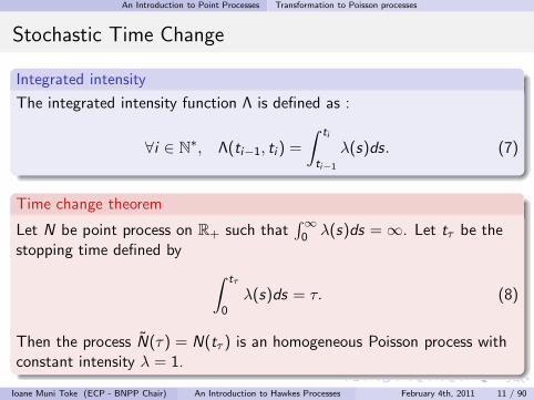
Stochastic Time Change
Integrated intensity
The integrated intensity function Λ is defined as :
∀i ∈ N∗, Λ(ti−1, ti ) =
∫ ti
ti−1
λ(s)ds. (7)
Time change theorem
Let N be point process on R+ such that∫∞
0 λ(s)ds =∞. Let tτ be thestopping time defined by
∫ tτ
0λ(s)ds = τ. (8)
Then the process N(τ) = N(tτ ) is an homogeneous Poisson process withconstant intensity λ = 1.
Ioane Muni Toke (ECP - BNPP Chair) An Introduction to Hawkes Processes February 4th, 2011 11 / 90
One-dimensional Hawkes processes
Table of contents
1 An Introduction to Point ProcessesBasic definitionsTransformation to Poisson processes
2 One-dimensional Hawkes processesDefinition and stationarity propertiesSimulation of a Hawkes processMaximum-likelihood estimation
3 Multidimensional Hawkes processesDefinition and stationarity conditionSimulation of a multivariate Hawkes processMaximum-likelihood estimation
4 A simple model for buy and sell intensities
5 Modelling microstructure noise
6 Some statistical findings about the order book
7 An order book model with Hawkes processes
Ioane Muni Toke (ECP - BNPP Chair) An Introduction to Hawkes Processes February 4th, 2011 12 / 90
One-dimensional Hawkes processes Definition and stationarity properties
Table of contents
1 An Introduction to Point ProcessesBasic definitionsTransformation to Poisson processes
2 One-dimensional Hawkes processesDefinition and stationarity propertiesSimulation of a Hawkes processMaximum-likelihood estimation
3 Multidimensional Hawkes processesDefinition and stationarity conditionSimulation of a multivariate Hawkes processMaximum-likelihood estimation
4 A simple model for buy and sell intensities
5 Modelling microstructure noise
6 Some statistical findings about the order book
7 An order book model with Hawkes processes
Ioane Muni Toke (ECP - BNPP Chair) An Introduction to Hawkes Processes February 4th, 2011 13 / 90

One-dimensional Hawkes processes Definition and stationarity properties
Definition of a linear self-exciting process
Linear self-exciting process
A general definition for a linear self-exciting process N reads :
λ(t) = λ0(t) +
∫ t
−∞
ν(t − s)dNs ,
= λ0(t) +∑
ti<t
ν(t − ti), (9)
where λ0 : R 7→ R+ is a deterministic base intensity and ν : R+ 7→ R+
expresses the positive influence of the past events ti on the current valueof the intensity process.
Ioane Muni Toke (ECP - BNPP Chair) An Introduction to Hawkes Processes February 4th, 2011 14 / 90
One-dimensional Hawkes processes Definition and stationarity properties
Simple Hawkes process considered here
Hawkes process
Hawkes (1971) proposes an exponential kernel ν(t) =∑P
j=1 αje−βj t1R+ ,
so that the intensity of the model becomes :
λ(t) = λ0(t) +
∫ t
0
P∑
j=1
αje−βj(t−s)dNs ,
= λ0(t) +∑
ti<t
P∑
j=1
αje−βj(t−ti ), (10)
The simplest version with P = 1 and λ0(t) constant is defined as:
λ(t) = λ0 +
∫ t
0αe−β(t−s)dNs = λ0 +
∑
ti<t
αe−β(t−ti ). (11)
Ioane Muni Toke (ECP - BNPP Chair) An Introduction to Hawkes Processes February 4th, 2011 15 / 90
One-dimensional Hawkes processes Definition and stationarity properties
Sample path of a 1D-Hawkes process
0
1
2
3
4
5
0 2 4 6 8 10
Time
Intensity maximum λ*
Intensity λEvents
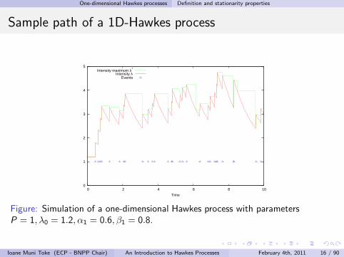
Figure: Simulation of a one-dimensional Hawkes process with parametersP = 1, λ0 = 1.2, α1 = 0.6, β1 = 0.8.
Ioane Muni Toke (ECP - BNPP Chair) An Introduction to Hawkes Processes February 4th, 2011 16 / 90
One-dimensional Hawkes processes Definition and stationarity properties
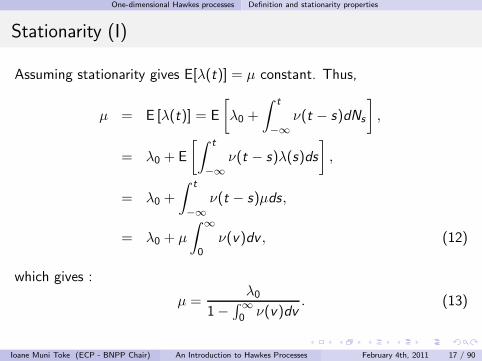
Stationarity (I)
Assuming stationarity gives E[λ(t)] = µ constant. Thus,
µ = E [λ(t)] = E
[
λ0 +
∫ t
−∞
ν(t − s)dNs
]
,
= λ0 + E
[∫ t
−∞
ν(t − s)λ(s)ds
]
,
= λ0 +
∫ t
−∞
ν(t − s)µds,
= λ0 + µ
∫ ∞
0ν(v)dv , (12)
which gives :
µ =λ0
1−∫∞
0 ν(v)dv. (13)
Ioane Muni Toke (ECP - BNPP Chair) An Introduction to Hawkes Processes February 4th, 2011 17 / 90
One-dimensional Hawkes processes Definition and stationarity properties
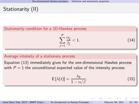
Stationarity (II)
Stationarity condition for a 1D-Hawkes process
P∑
j=1
αj
βj< 1. (14)
Average intensity of a stationary process
Equation (13) immediately gives for the one-dimensional Hawkes processwith P = 1 the unconditional expected value of the intensity process:
E [λ(t)] =λ0
1− α/β. (15)
Ioane Muni Toke (ECP - BNPP Chair) An Introduction to Hawkes Processes February 4th, 2011 18 / 90
One-dimensional Hawkes processes Simulation of a Hawkes process
Table of contents
1 An Introduction to Point ProcessesBasic definitionsTransformation to Poisson processes
2 One-dimensional Hawkes processesDefinition and stationarity propertiesSimulation of a Hawkes processMaximum-likelihood estimation
3 Multidimensional Hawkes processesDefinition and stationarity conditionSimulation of a multivariate Hawkes processMaximum-likelihood estimation
4 A simple model for buy and sell intensities
5 Modelling microstructure noise
6 Some statistical findings about the order book
7 An order book model with Hawkes processes
Ioane Muni Toke (ECP - BNPP Chair) An Introduction to Hawkes Processes February 4th, 2011 19 / 90
One-dimensional Hawkes processes Simulation of a Hawkes process
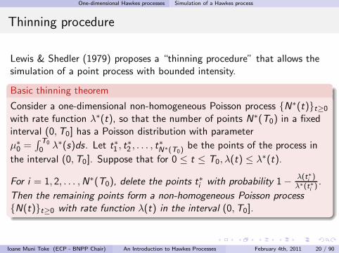
Thinning procedure
Lewis & Shedler (1979) proposes a “thinning procedure” that allows thesimulation of a point process with bounded intensity.
Basic thinning theorem
Consider a one-dimensional non-homogeneous Poisson process N∗(t)t≥0
with rate function λ∗(t), so that the number of points N∗(T0) in a fixedinterval (0,T0] has a Poisson distribution with parameter
µ∗0 =
∫ T0
0 λ∗(s)ds. Let t∗1 , t∗2 , . . . , t
∗N∗(T0)
be the points of the process in
the interval (0,T0]. Suppose that for 0 ≤ t ≤ T0, λ(t) ≤ λ∗(t).
For i = 1, 2, . . . ,N∗(T0), delete the points t∗i with probability 1− λ(t∗i)
λ∗(t∗i) .
Then the remaining points form a non-homogeneous Poisson process
N(t)t≥0 with rate function λ(t) in the interval (0,T0].
Ioane Muni Toke (ECP - BNPP Chair) An Introduction to Hawkes Processes February 4th, 2011 20 / 90
One-dimensional Hawkes processes Simulation of a Hawkes process
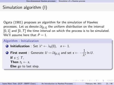
Simulation algorithm (I)
Ogata (1981) proposes an algorithm for the simulation of Hawkesprocesses. Let us denote U[0,1] the uniform distribution on the interval[0, 1] and [0,T ] the time interval on which the process is to be simulated.We’ll assume here that P = 1.
Algorithm - Initialization
1 Initialization : Set λ∗ ← λ0(0), n← 1.
2 First event : Generate U U[0,1] and set s ← − 1
λ∗lnU.
If s ≤ T ,Then t1 ← s,Else go to last step.
Ioane Muni Toke (ECP - BNPP Chair) An Introduction to Hawkes Processes February 4th, 2011 21 / 90
One-dimensional Hawkes processes Simulation of a Hawkes process
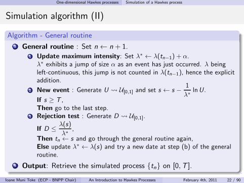
Simulation algorithm (II)
Algorithm - General routine
3 General routine : Set n← n + 1.1 Update maximum intensity: Set λ∗ ← λ(tn−1) + α.
λ∗ exhibits a jump of size α as an event has just occurred. λ beingleft-continuous, this jump is not counted in λ(tn−1), hence the explicitaddition.
2 New event : Generate U U[0,1] and set s ← s − 1
λ∗lnU .
If s ≥ T ,Then go to the last step.
3 Rejection test : Generate D U[0,1].If D ≤ λ(s)
λ∗,
Then tn ← s and go through the general routine again,Else update λ∗ ← λ(s) and try a new date at step (b) of the generalroutine.
4 Output: Retrieve the simulated process tn on [0,T ].
Ioane Muni Toke (ECP - BNPP Chair) An Introduction to Hawkes Processes February 4th, 2011 22 / 90
One-dimensional Hawkes processes Simulation of a Hawkes process
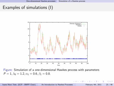
Examples of simulations (I)
0
2
4
6
8
10
12
0 10 20 30 40 50 60 70 80 90 100
Time
Intensity maximum λ*
Intensity λEvents
Figure: Simulation of a one-dimensional Hawkes process with parametersP = 1, λ0 = 1.2, α1 = 0.6, β1 = 0.8.
Ioane Muni Toke (ECP - BNPP Chair) An Introduction to Hawkes Processes February 4th, 2011 23 / 90
One-dimensional Hawkes processes Simulation of a Hawkes process
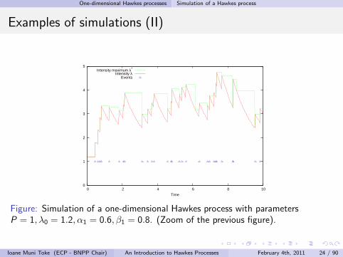
Examples of simulations (II)
0
1
2
3
4
5
0 2 4 6 8 10
Time
Intensity maximum λ*
Intensity λEvents
Figure: Simulation of a one-dimensional Hawkes process with parametersP = 1, λ0 = 1.2, α1 = 0.6, β1 = 0.8. (Zoom of the previous figure).
Ioane Muni Toke (ECP - BNPP Chair) An Introduction to Hawkes Processes February 4th, 2011 24 / 90
One-dimensional Hawkes processes Simulation of a Hawkes process
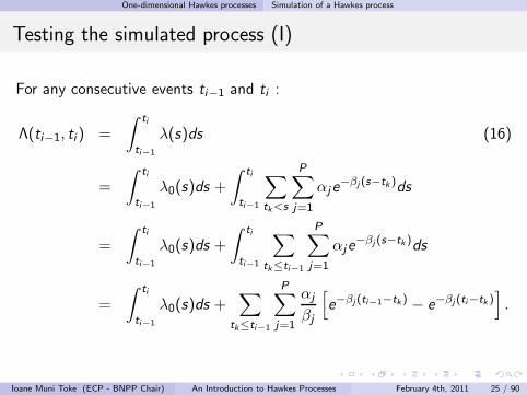
Testing the simulated process (I)
For any consecutive events ti−1 and ti :
Λ(ti−1, ti ) =
∫ ti
ti−1
λ(s)ds (16)
=
∫ ti
ti−1
λ0(s)ds +
∫ ti
ti−1
∑
tk<s
P∑
j=1
αje−βj (s−tk )ds
=
∫ ti
ti−1
λ0(s)ds +
∫ ti
ti−1
∑
tk≤ti−1
P∑
j=1
αje−βj (s−tk )ds
=
∫ ti
ti−1
λ0(s)ds +∑
tk≤ti−1
P∑
j=1
αj
βj
[
e−βj (ti−1−tk) − e−βj (ti−tk )]
.
Ioane Muni Toke (ECP - BNPP Chair) An Introduction to Hawkes Processes February 4th, 2011 25 / 90
One-dimensional Hawkes processes Simulation of a Hawkes process
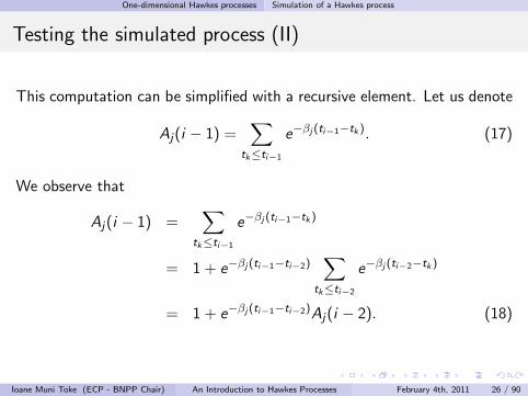
Testing the simulated process (II)
This computation can be simplified with a recursive element. Let us denote
Aj(i − 1) =∑
tk≤ti−1
e−βj (ti−1−tk). (17)
We observe that
Aj(i − 1) =∑
tk≤ti−1
e−βj (ti−1−tk)
= 1 + e−βj (ti−1−ti−2)∑
tk≤ti−2
e−βj (ti−2−tk )
= 1 + e−βj (ti−1−ti−2)Aj(i − 2). (18)
Ioane Muni Toke (ECP - BNPP Chair) An Introduction to Hawkes Processes February 4th, 2011 26 / 90
One-dimensional Hawkes processes Simulation of a Hawkes process
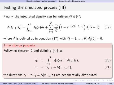
Testing the simulated process (III)
Finally, the integrated density can be written ∀i ∈ N∗:
Λ(ti−1, ti ) =
∫ ti
ti−1
λ0(s)ds +
P∑
j=1
αj
βj
(
1− e−βj(ti−ti−1))
Aj(i − 1), (19)
where A is defined as in equation (17) with ∀j = 1, . . . ,P ,Aj(0) = 0.
Time change property
Following theorem 2 and defining τi as
τ0 =
∫ t0
0λ(s)ds = Λ(0, t0), (20)
τi = τi−1 + Λ(ti−1, ti ), (21)
the durations τi − τi−1 = Λ(ti−1, ti ) are exponentially distributed.
Ioane Muni Toke (ECP - BNPP Chair) An Introduction to Hawkes Processes February 4th, 2011 27 / 90
One-dimensional Hawkes processes Simulation of a Hawkes process
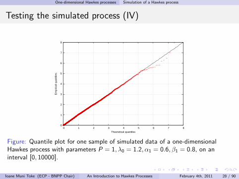
Testing the simulated process (IV)
0
1
2
3
4
5
6
7
8
0 1 2 3 4 5 6 7 8
Em
piric
al q
uant
iles
Theoretical quantiles
Figure: Quantile plot for one sample of simulated data of a one-dimensionalHawkes process with parameters P = 1, λ0 = 1.2, α1 = 0.6, β1 = 0.8, on aninterval [0, 10000].
Ioane Muni Toke (ECP - BNPP Chair) An Introduction to Hawkes Processes February 4th, 2011 28 / 90
One-dimensional Hawkes processes Maximum-likelihood estimation
Table of contents
1 An Introduction to Point ProcessesBasic definitionsTransformation to Poisson processes
2 One-dimensional Hawkes processesDefinition and stationarity propertiesSimulation of a Hawkes processMaximum-likelihood estimation
3 Multidimensional Hawkes processesDefinition and stationarity conditionSimulation of a multivariate Hawkes processMaximum-likelihood estimation
4 A simple model for buy and sell intensities
5 Modelling microstructure noise
6 Some statistical findings about the order book
7 An order book model with Hawkes processes
Ioane Muni Toke (ECP - BNPP Chair) An Introduction to Hawkes Processes February 4th, 2011 29 / 90
One-dimensional Hawkes processes Maximum-likelihood estimation
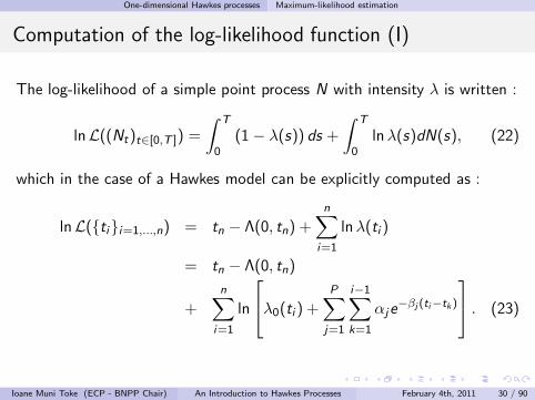
Computation of the log-likelihood function (I)
The log-likelihood of a simple point process N with intensity λ is written :
lnL((Nt)t∈[0,T ]) =
∫ T
0(1− λ(s)) ds +
∫ T
0lnλ(s)dN(s), (22)
which in the case of a Hawkes model can be explicitly computed as :
lnL(tii=1,...,n) = tn − Λ(0, tn) +
n∑
i=1
lnλ(ti )
= tn − Λ(0, tn)
+
n∑
i=1
ln
λ0(ti ) +
P∑
j=1
i−1∑
k=1
αje−βj (ti−tk)
. (23)
Ioane Muni Toke (ECP - BNPP Chair) An Introduction to Hawkes Processes February 4th, 2011 30 / 90
One-dimensional Hawkes processes Maximum-likelihood estimation
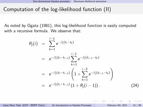
Computation of the log-likelihood function (II)
As noted by Ogata (1981), this log-likelihood function is easily computedwith a recursive formula. We observe that:
Rj(i) =
i−1∑
k=1
e−βj (ti−tk )
= e−βj (ti−ti−1)i−1∑
k=1
e−βj (ti−1−tk )
= e−βj (ti−ti−1)
(
1 +i−2∑
k=1
e−βj (ti−1−tk)
)
= e−βj (ti−ti−1) (1 + Rj(i − 1)) . (24)
Ioane Muni Toke (ECP - BNPP Chair) An Introduction to Hawkes Processes February 4th, 2011 31 / 90
One-dimensional Hawkes processes Maximum-likelihood estimation
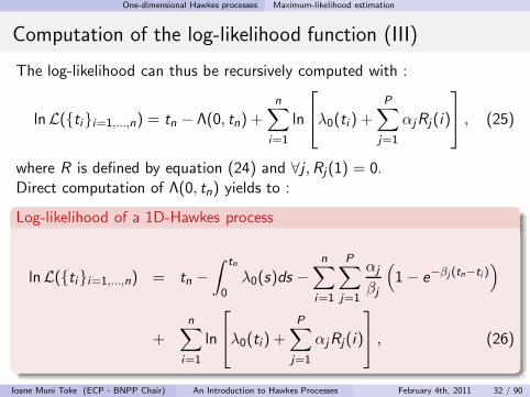
Computation of the log-likelihood function (III)
The log-likelihood can thus be recursively computed with :
lnL(tii=1,...,n) = tn − Λ(0, tn) +
n∑
i=1
ln
λ0(ti ) +
P∑
j=1
αjRj(i)
, (25)
where R is defined by equation (24) and ∀j ,Rj(1) = 0.Direct computation of Λ(0, tn) yields to :
Log-likelihood of a 1D-Hawkes process
lnL(tii=1,...,n) = tn −∫ tn
0λ0(s)ds −
n∑
i=1
P∑
j=1
αj
βj
(
1− e−βj (tn−ti ))
+
n∑
i=1
ln
λ0(ti ) +
P∑
j=1
αjRj(i)
, (26)
Ioane Muni Toke (ECP - BNPP Chair) An Introduction to Hawkes Processes February 4th, 2011 32 / 90
One-dimensional Hawkes processes Maximum-likelihood estimation
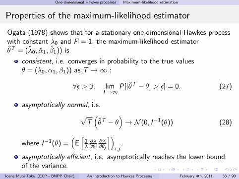
Properties of the maximum-likelihood estimator
Ogata (1978) shows that for a stationary one-dimensional Hawkes processwith constant λ0 and P = 1, the maximum-likelihood estimatorθT = (λ0, α1, β1)) is
consistent, i.e. converges in probability to the true valuesθ = (λ0, α1, β1)) as T →∞ :
∀ǫ > 0, limT→∞
P [|θT − θ| > ǫ] = 0. (27)
asymptotically normal, i.e.
√T(
θT − θ)
→ N (0, I−1(θ)) (28)
where I−1(θ) =(
E[
1λ
∂λ∂θi
∂λ∂θj
])
i ,j.
asymptotically efficient, i.e. asymptotically reaches the lower boundof the variance.
Ioane Muni Toke (ECP - BNPP Chair) An Introduction to Hawkes Processes February 4th, 2011 33 / 90
One-dimensional Hawkes processes Maximum-likelihood estimation
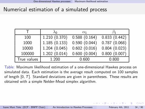
Numerical estimation of a simulated process
T λ0 α1 β1100 1.210 (0.370) 0.588 (0.164) 0.833 (0.442)1000 1.185 (0.133) 0.590 (0.044) 0.787 (0.068)10000 1.204 (0.045) 0.602 (0.016) 0.804 (0.023)100000 1.202 (0.014) 0.600 (0.004) 0.800 (0.007)
True values 1.200 0.600 0.800
Table: Maximum likelihood estimation of a one-dimensional Hawkes process onsimulated data. Each estimation is the average result computed on 100 samplesof length [0,T ]. Standard deviations are given in parentheses. These results areobtained with a simple Nelder-Mead simplex algorithm.
Ioane Muni Toke (ECP - BNPP Chair) An Introduction to Hawkes Processes February 4th, 2011 34 / 90
Multidimensional Hawkes processes
Table of contents
1 An Introduction to Point ProcessesBasic definitionsTransformation to Poisson processes
2 One-dimensional Hawkes processesDefinition and stationarity propertiesSimulation of a Hawkes processMaximum-likelihood estimation
3 Multidimensional Hawkes processesDefinition and stationarity conditionSimulation of a multivariate Hawkes processMaximum-likelihood estimation
4 A simple model for buy and sell intensities
5 Modelling microstructure noise
6 Some statistical findings about the order book
7 An order book model with Hawkes processes
Ioane Muni Toke (ECP - BNPP Chair) An Introduction to Hawkes Processes February 4th, 2011 35 / 90
Multidimensional Hawkes processes Definition and stationarity condition
Table of contents
1 An Introduction to Point ProcessesBasic definitionsTransformation to Poisson processes
2 One-dimensional Hawkes processesDefinition and stationarity propertiesSimulation of a Hawkes processMaximum-likelihood estimation
3 Multidimensional Hawkes processesDefinition and stationarity conditionSimulation of a multivariate Hawkes processMaximum-likelihood estimation
4 A simple model for buy and sell intensities
5 Modelling microstructure noise
6 Some statistical findings about the order book
7 An order book model with Hawkes processes
Ioane Muni Toke (ECP - BNPP Chair) An Introduction to Hawkes Processes February 4th, 2011 36 / 90
Multidimensional Hawkes processes Definition and stationarity condition
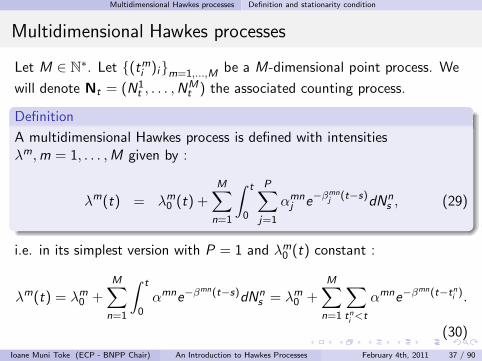
Multidimensional Hawkes processes
Let M ∈ N∗. Let (tmi )im=1,...,M be a M-dimensional point process. We
will denote Nt = (N1t , . . . ,N
Mt ) the associated counting process.
Definition
A multidimensional Hawkes process is defined with intensitiesλm,m = 1, . . . ,M given by :
λm(t) = λm0 (t) +
M∑
n=1
∫ t
0
P∑
j=1
αmnj e
−βmnj
(t−s)dNn
s , (29)
i.e. in its simplest version with P = 1 and λm0 (t) constant :
λm(t) = λm0 +
M∑
n=1
∫ t
0αmne−βmn(t−s)dNn
s = λm0 +
M∑
n=1
∑
tni<t
αmne−βmn(t−tni ).
(30)
Ioane Muni Toke (ECP - BNPP Chair) An Introduction to Hawkes Processes February 4th, 2011 37 / 90
Multidimensional Hawkes processes Definition and stationarity condition
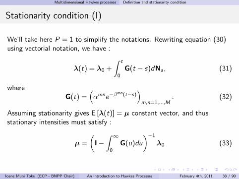
Stationarity condition (I)
We’ll take here P = 1 to simplify the notations. Rewriting equation (30)using vectorial notation, we have :
λ(t) = λ0 +
∫ t
0G(t − s)dNs , (31)
whereG(t) =
(
αmne−βmn(t−s))
m,n=1,...,M. (32)
Assuming stationarity gives E [λ(t)] = µ constant vector, and thusstationary intensities must satisfy :
µ =
(
I−∫ ∞
0G(u)du
)−1
λ0 (33)
Ioane Muni Toke (ECP - BNPP Chair) An Introduction to Hawkes Processes February 4th, 2011 38 / 90
Multidimensional Hawkes processes Definition and stationarity condition
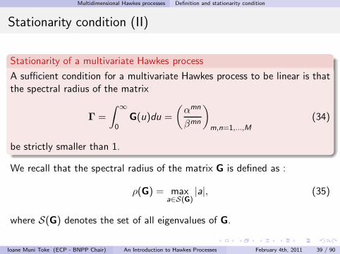
Stationarity condition (II)
Stationarity of a multivariate Hawkes process
A sufficient condition for a multivariate Hawkes process to be linear is thatthe spectral radius of the matrix
Γ =
∫ ∞
0G(u)du =
(
αmn
βmn
)
m,n=1,...,M
(34)
be strictly smaller than 1.
We recall that the spectral radius of the matrix G is defined as :
ρ(G) = maxa∈S(G)
|a|, (35)
where S(G) denotes the set of all eigenvalues of G.
Ioane Muni Toke (ECP - BNPP Chair) An Introduction to Hawkes Processes February 4th, 2011 39 / 90
Multidimensional Hawkes processes Simulation of a multivariate Hawkes process
Table of contents
1 An Introduction to Point ProcessesBasic definitionsTransformation to Poisson processes
2 One-dimensional Hawkes processesDefinition and stationarity propertiesSimulation of a Hawkes processMaximum-likelihood estimation
3 Multidimensional Hawkes processesDefinition and stationarity conditionSimulation of a multivariate Hawkes processMaximum-likelihood estimation
4 A simple model for buy and sell intensities
5 Modelling microstructure noise
6 Some statistical findings about the order book
7 An order book model with Hawkes processes
Ioane Muni Toke (ECP - BNPP Chair) An Introduction to Hawkes Processes February 4th, 2011 40 / 90
Multidimensional Hawkes processes Simulation of a multivariate Hawkes process
Simulation of a multivariate Hawkes process (I)
We generalize the 1D-algorithm in a multidimensional setting. We recallthat :
U[0,1] denotes the uniform distribution on the interval [0, 1],
[0,T ] is the time interval on which the process is to be simulated,
and we define
IK (t) =
K∑
n=1
λn(t) (36)
the sum of the intensities of the first K components of the multivariateprocess. IM(t) =
∑Mn=1 λ
n(t) is thus the total intensity of the multivariateprocess and we set I 0 = 0. The algorithm is then rewritten as follows.
Ioane Muni Toke (ECP - BNPP Chair) An Introduction to Hawkes Processes February 4th, 2011 41 / 90
Multidimensional Hawkes processes Simulation of a multivariate Hawkes process
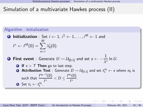
Simulation of a multivariate Hawkes process (II)
Algorithm - Initialization
1 Initialization : Set i ← 1, i1 ← 1, . . . , iM ← 1 and
I ∗ ← IM(0) =M∑
n=i
λi0(0).
2 First event : Generate U U[0,1] and set s ← − 1
λ∗lnU.
1 If s > T Then go to last step.2 Attribution Test : Generate D U[0,1] and set tn01 ← s where n0 is
such thatI n0−1(0)
I ∗< D ≤ I n0(0)
I ∗.
3 Set t1 ← tn01 .
Ioane Muni Toke (ECP - BNPP Chair) An Introduction to Hawkes Processes February 4th, 2011 42 / 90
Multidimensional Hawkes processes Simulation of a multivariate Hawkes process
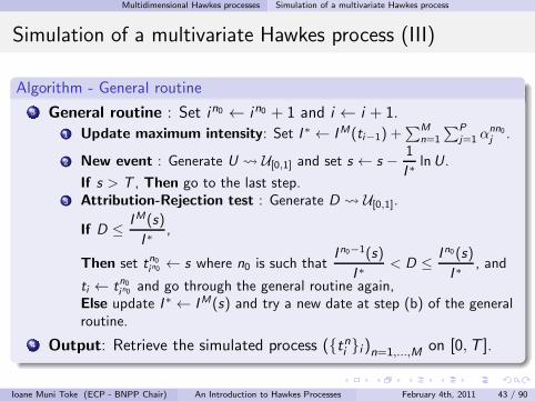
Simulation of a multivariate Hawkes process (III)
Algorithm - General routine
3 General routine : Set in0 ← in0 + 1 and i ← i + 1.1 Update maximum intensity: Set I ∗ ← IM(ti−1) +
∑M
n=1
∑P
j=1 αnn0j .
2 New event : Generate U U[0,1] and set s ← s − 1
I ∗lnU .
If s > T , Then go to the last step.3 Attribution-Rejection test : Generate D U[0,1].
If D ≤ IM(s)
I ∗,
Then set tn0in0 ← s where n0 is such thatI n0−1(s)
I ∗< D ≤ I n0(s)
I ∗, and
ti ← tn0in0 and go through the general routine again,Else update I ∗ ← IM(s) and try a new date at step (b) of the generalroutine.
4 Output: Retrieve the simulated process (tni i )n=1,...,M on [0,T ].
Ioane Muni Toke (ECP - BNPP Chair) An Introduction to Hawkes Processes February 4th, 2011 43 / 90
Multidimensional Hawkes processes Simulation of a multivariate Hawkes process
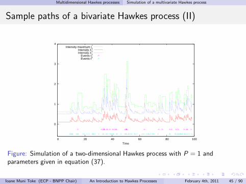
Sample paths of a bivariate Hawkes process (I)
We simulate a bivariate Hawkes process with P = 1 and the followingparameters:
λ10 = 0.1, α11
1 = 0.2, β111 = 1.0, α12
1 = 0.1, β121 = 1.0,
λ20 = 0.5, α21
1 = 0.5, β211 = 1.0, α22
1 = 0.1, β221 = 1.0, (37)
Ioane Muni Toke (ECP - BNPP Chair) An Introduction to Hawkes Processes February 4th, 2011 44 / 90
Multidimensional Hawkes processes Simulation of a multivariate Hawkes process
Sample paths of a bivariate Hawkes process (II)
0
1
2
3
4
0 20 40 60 80 100
Time
Intensity maximum I*
Intensity λ1
Intensity λ2
Events t1
Events t2
Figure: Simulation of a two-dimensional Hawkes process with P = 1 andparameters given in equation (37).
Ioane Muni Toke (ECP - BNPP Chair) An Introduction to Hawkes Processes February 4th, 2011 45 / 90
Multidimensional Hawkes processes Simulation of a multivariate Hawkes process
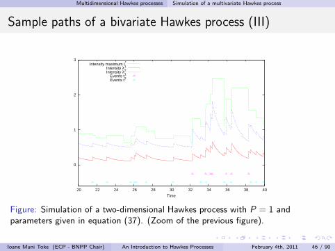
Sample paths of a bivariate Hawkes process (III)
0
1
2
3
20 22 24 26 28 30 32 34 36 38 40
Time
Intensity maximum I*
Intensity λ1
Intensity λ2
Events t1
Events t2
Figure: Simulation of a two-dimensional Hawkes process with P = 1 andparameters given in equation (37). (Zoom of the previous figure).
Ioane Muni Toke (ECP - BNPP Chair) An Introduction to Hawkes Processes February 4th, 2011 46 / 90
Multidimensional Hawkes processes Simulation of a multivariate Hawkes process
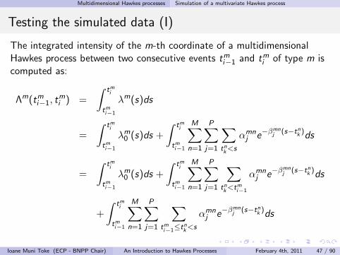
Testing the simulated data (I)
The integrated intensity of the m-th coordinate of a multidimensionalHawkes process between two consecutive events tmi−1 and tmi of type m iscomputed as:
Λm(tmi−1, tmi ) =
∫ tmi
tmi−1
λm(s)ds
=
∫ tmi
tmi−1
λm0 (s)ds +
∫ tmi
tmi−1
M∑
n=1
P∑
j=1
∑
tnk<s
αmnj e
−βmnj (s−tn
k)ds
=
∫ tmi
tmi−1
λm0 (s)ds +
∫ tmi
tmi−1
M∑
n=1
P∑
j=1
∑
tnk<tm
i−1
αmnj e
−βmnj (s−tn
k)ds
+
∫ tmi
tmi−1
M∑
n=1
P∑
j=1
∑
tmi−1≤tn
k<s
αmnj e
−βmnj
(s−tnk)ds
Ioane Muni Toke (ECP - BNPP Chair) An Introduction to Hawkes Processes February 4th, 2011 47 / 90
Multidimensional Hawkes processes Simulation of a multivariate Hawkes process
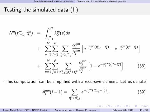
Testing the simulated data (II)
Λm(tmi−1, tmi ) =
∫ tmi
tmi−1
λm0 (s)ds
+
M∑
n=1
P∑
j=1
∑
tnk<tm
i−1
αmnj
βmnj
[
e−βmn
j (tmi−1−tnk) − e
−βmnj (tmi −tn
k)]
+M∑
n=1
P∑
j=1
∑
tmi−1≤tn
k<tm
i
αmnj
βmnj
[
1− e−βmn
j(tm
i−tn
k)]
. (38)
This computation can be simplified with a recursive element. Let us denote
Amnj (i − 1) =
∑
tnk<tm
i−1
e−βmn
j(tm
i−1−tnk). (39)
Ioane Muni Toke (ECP - BNPP Chair) An Introduction to Hawkes Processes February 4th, 2011 48 / 90
Multidimensional Hawkes processes Simulation of a multivariate Hawkes process
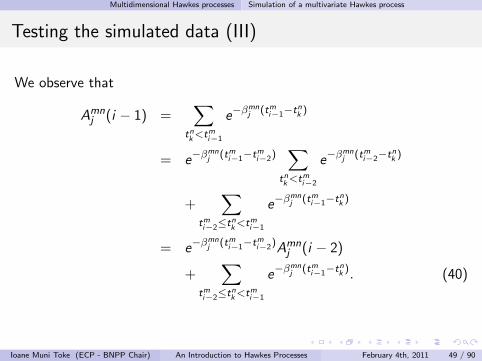
Testing the simulated data (III)
We observe that
Amnj (i − 1) =
∑
tnk<tm
i−1
e−βmn
j (tmi−1−tnk)
= e−βmn
j (tmi−1−tmi−2)∑
tnk<tm
i−2
e−βmn
j (tmi−2−tnk)
+∑
tmi−2≤tn
k<tm
i−1
e−βmn
j (tmi−1−tnk)
= e−βmn
j(tm
i−1−tmi−2)Amn
j (i − 2)
+∑
tmi−2≤tn
k<tm
i−1
e−βmn
j(tm
i−1−tnk). (40)
Ioane Muni Toke (ECP - BNPP Chair) An Introduction to Hawkes Processes February 4th, 2011 49 / 90
Multidimensional Hawkes processes Simulation of a multivariate Hawkes process
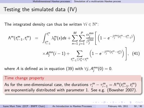
Testing the simulated data (IV)
The integrated density can thus be written ∀i ∈ N∗:
Λm(tmi−1, tmi ) =
∫ tmi
tmi−1
λm0 (s)ds +
M∑
n=1
P∑
j=1
αmnj
βmnj
[
(
1− e−βmn
j(tm
i−tm
i−1))
×Amnj (i − 1) +
∑
tmi−1≤tn
k<tm
i
(
1− e−βmn
j(tm
i−tn
k))
]
, (41)
where A is defined as in equation (39) with ∀j ,Amnj (0) = 0.
Time change property
As for the one-dimensional case, the durations τmi − τmi−1 = Λm(tmi−1, tmi )
are exponentially distributed with parameter 1. See e.g. (Bowsher 2007).
Ioane Muni Toke (ECP - BNPP Chair) An Introduction to Hawkes Processes February 4th, 2011 50 / 90
Multidimensional Hawkes processes Simulation of a multivariate Hawkes process
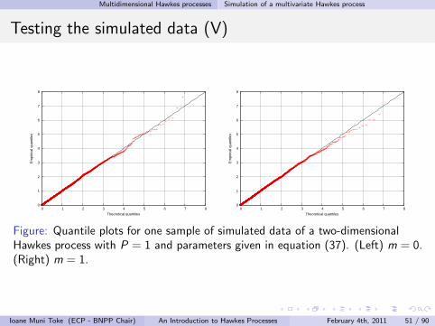
Testing the simulated data (V)
0
1
2
3
4
5
6
7
8
0 1 2 3 4 5 6 7 8
Em
piric
al q
uant
iles
Theoretical quantiles
0
1
2
3
4
5
6
7
8
0 1 2 3 4 5 6 7 8
Em
piric
al q
uant
iles
Theoretical quantiles
Figure: Quantile plots for one sample of simulated data of a two-dimensionalHawkes process with P = 1 and parameters given in equation (37). (Left) m = 0.(Right) m = 1.
Ioane Muni Toke (ECP - BNPP Chair) An Introduction to Hawkes Processes February 4th, 2011 51 / 90
Multidimensional Hawkes processes Maximum-likelihood estimation
Table of contents
1 An Introduction to Point ProcessesBasic definitionsTransformation to Poisson processes
2 One-dimensional Hawkes processesDefinition and stationarity propertiesSimulation of a Hawkes processMaximum-likelihood estimation
3 Multidimensional Hawkes processesDefinition and stationarity conditionSimulation of a multivariate Hawkes processMaximum-likelihood estimation
4 A simple model for buy and sell intensities
5 Modelling microstructure noise
6 Some statistical findings about the order book
7 An order book model with Hawkes processes
Ioane Muni Toke (ECP - BNPP Chair) An Introduction to Hawkes Processes February 4th, 2011 52 / 90
Multidimensional Hawkes processes Maximum-likelihood estimation
Computation of the log-likelihood function (I)
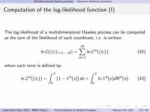
The log-likelihood of a multidimensional Hawkes process can be computedas the sum of the likelihood of each coordinate, i.e. is written:
lnL(tii=1,...,N) =
M∑
m=1
lnLm(ti), (42)
where each term is defined by:
lnLm(ti) =∫ T
0(1− λm(s)) ds +
∫ T
0lnλm(s)dNm(s). (43)
Ioane Muni Toke (ECP - BNPP Chair) An Introduction to Hawkes Processes February 4th, 2011 53 / 90
Multidimensional Hawkes processes Maximum-likelihood estimation
Computation of the log-likelihood function (II)
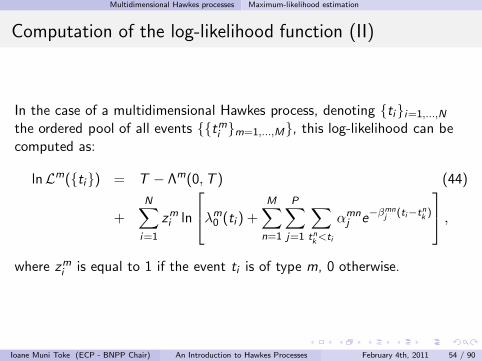
In the case of a multidimensional Hawkes process, denoting tii=1,...,N
the ordered pool of all events tmi m=1,...,M, this log-likelihood can becomputed as:
lnLm(ti) = T − Λm(0,T ) (44)
+
N∑
i=1
zmi ln
λm0 (ti ) +
M∑
n=1
P∑
j=1
∑
tnk<ti
αmnj e
−βmnj (ti−tn
k)
,
where zmi is equal to 1 if the event ti is of type m, 0 otherwise.
Ioane Muni Toke (ECP - BNPP Chair) An Introduction to Hawkes Processes February 4th, 2011 54 / 90
Multidimensional Hawkes processes Maximum-likelihood estimation
Computation of the log-likelihood function (III)
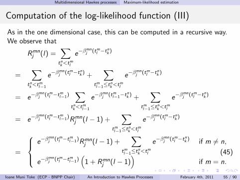
As in the one dimensional case, this can be computed in a recursive way.We observe that
Rmnj (l) =
∑
tnk<tm
l
e−βmn
j (tml−tn
k)
=∑
tnk<tm
l−1
e−βmn
j(tm
l−tn
k) +
∑
tml−1≤tn
k<tm
l
e−βmn
j(tm
l−tn
k)
= e−βmn
j (tml−tm
l−1)∑
tnk<tm
l−1
e−βmn
j (tml−1−tn
k) +
∑
tml−1≤tn
k<tm
l
e−βmn
j (tml−tn
k)
= e−βmn
j(tm
l−tm
l−1)Rmnj (l − 1) +
∑
tml−1≤tn
k<tm
l
e−βmn
j(tm
l−tn
k)
=
e−βmn
j (tml−tm
l−1)Rmnj (l − 1) +
∑
tml−1≤tn
k<tm
l
e−βmn
j (tml−tn
k) if m 6= n,
e−βmn
j(tm
l−tm
l−1)(
1 + Rmnj (l − 1)
)
if m = n.
(45)
Ioane Muni Toke (ECP - BNPP Chair) An Introduction to Hawkes Processes February 4th, 2011 55 / 90
Multidimensional Hawkes processes Maximum-likelihood estimation
Computation of the log-likelihood function (IV)
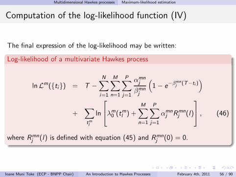
The final expression of the log-likelihood may be written:
Log-likelihood of a multivariate Hawkes process
lnLm(ti) = T −N∑
i=1
M∑
n=1
P∑
j=1
αmnj
βmnj
(
1− e−βmn
j (T−ti ))
+∑
tml
ln
λm0 (t
ml ) +
M∑
n=1
P∑
j=1
αmnj Rmn
j (l)
, (46)
where Rmnj (l) is defined with equation (45) and Rmn
j (0) = 0.
Ioane Muni Toke (ECP - BNPP Chair) An Introduction to Hawkes Processes February 4th, 2011 56 / 90
Multidimensional Hawkes processes Maximum-likelihood estimation
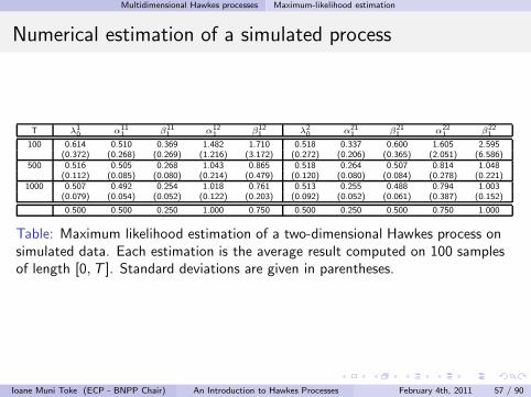
Numerical estimation of a simulated process
T λ10 α11
1 β111 α12
1 β121 λ2
0 α211 β21
1 α221 β22
1
100 0.614 0.510 0.369 1.482 1.710 0.518 0.337 0.600 1.605 2.595(0.372) (0.268) (0.269) (1.216) (3.172) (0.272) (0.206) (0.365) (2.051) (6.586)
500 0.516 0.505 0.268 1.043 0.865 0.518 0.264 0.507 0.814 1.048(0.112) (0.085) (0.080) (0.214) (0.479) (0.120) (0.080) (0.084) (0.278) (0.221)
1000 0.507 0.492 0.254 1.018 0.761 0.513 0.255 0.488 0.794 1.003(0.079) (0.054) (0.052) (0.122) (0.203) (0.092) (0.052) (0.061) (0.387) (0.152)
0.500 0.500 0.250 1.000 0.750 0.500 0.250 0.500 0.750 1.000
Table: Maximum likelihood estimation of a two-dimensional Hawkes process onsimulated data. Each estimation is the average result computed on 100 samplesof length [0,T ]. Standard deviations are given in parentheses.
Ioane Muni Toke (ECP - BNPP Chair) An Introduction to Hawkes Processes February 4th, 2011 57 / 90
A simple model for buy and sell intensities
Table of contents
1 An Introduction to Point ProcessesBasic definitionsTransformation to Poisson processes
2 One-dimensional Hawkes processesDefinition and stationarity propertiesSimulation of a Hawkes processMaximum-likelihood estimation
3 Multidimensional Hawkes processesDefinition and stationarity conditionSimulation of a multivariate Hawkes processMaximum-likelihood estimation
4 A simple model for buy and sell intensities
5 Modelling microstructure noise
6 Some statistical findings about the order book
7 An order book model with Hawkes processes
Ioane Muni Toke (ECP - BNPP Chair) An Introduction to Hawkes Processes February 4th, 2011 58 / 90
A simple model for buy and sell intensities
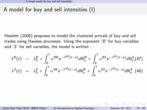
A model for buy and sell intensities (I)
Hewlett (2006) proposes to model the clustered arrivals of buy and selltrades using Hawkes processes. Using the exponent ’B ’ for buy variablesand ’S ’ for sell variables, the model is written :
λB(t) = λB0 +
∫ t
0αBBe−βBB (t−u)dNB
u +
∫ t
0αBSe−βBS (t−u)dNS
u ,(47)
λS(t) = λS0 +
∫ t
0αSBe−βSB (t−u)dNB
u +
∫ t
0αSSe−βSS (t−u)dNS
u . (48)
Ioane Muni Toke (ECP - BNPP Chair) An Introduction to Hawkes Processes February 4th, 2011 59 / 90
A simple model for buy and sell intensities
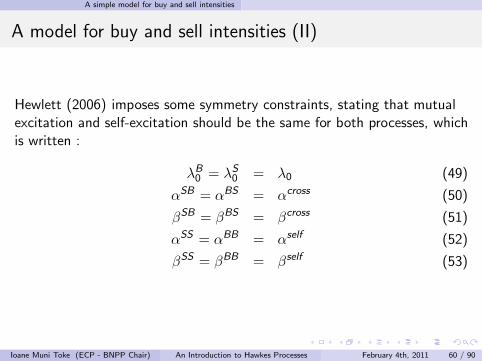
A model for buy and sell intensities (II)
Hewlett (2006) imposes some symmetry constraints, stating that mutualexcitation and self-excitation should be the same for both processes, whichis written :
λB0 = λS
0 = λ0 (49)
αSB = αBS = αcross (50)
βSB = βBS = βcross (51)
αSS = αBB = αself (52)
βSS = βBB = βself (53)
Ioane Muni Toke (ECP - BNPP Chair) An Introduction to Hawkes Processes February 4th, 2011 60 / 90
A simple model for buy and sell intensities
Goodness of fit
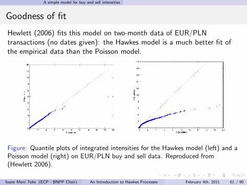
Hewlett (2006) fits this model on two-month data of EUR/PLNtransactions (no dates given): the Hawkes model is a much better fit ofthe empirical data than the Poisson model.
Figure: Quantile plots of integrated intensities for the Hawkes model (left) and aPoisson model (right) on EUR/PLN buy and sell data. Reproduced from(Hewlett 2006).
Ioane Muni Toke (ECP - BNPP Chair) An Introduction to Hawkes Processes February 4th, 2011 61 / 90
A simple model for buy and sell intensities
Numerical results
The numerical values obtained are :
λ0 = 0.0033, αcross = 0, αself = 0.0169, βself = 0.0286. (54)
In other words,
the occurrence of a buy (resp. sell) order has an exciting effect on thestream of buy (resp. sell) orders, with a typical half-life of ln 2
βself ≈ 24seconds;
the zero value of αcross tends to indicate that there is no influence ofbuy orders on sell orders, and conversely.
Ioane Muni Toke (ECP - BNPP Chair) An Introduction to Hawkes Processes February 4th, 2011 62 / 90
A simple model for buy and sell intensities
Test on our own data (I)
We perform the fit of a bivariate Hawkes model on buy/sell market orderson the following data : BNPP.PA, Feb. 1st 2010 to Feb. 23rd, 2010 (14trading days), 10am-12am without symmetry constraints. Numericalresults are :
λB0 = 0.080, αBB = 3.230, βBB = 13.304, αBS = 0.276, βBS = 6.193
λB0 = 0.086, αSB = 0.515, βSB = 13.451, αSS = 3.789, βSS = 14.151
Confirmation of the very limited cross-excitation effect.
Change of magnitude of parameters β: difference in precision of data(second, millisecond)
Ioane Muni Toke (ECP - BNPP Chair) An Introduction to Hawkes Processes February 4th, 2011 63 / 90
A simple model for buy and sell intensities
Test on our own data (II)
0
2
4
6
8
10
12
14
0 1 2 3 4 5 6 7
Day 0Day 1Day 2Day 3Day 4Day 5Day 6Day 7Day 8Day 9
Day 10Day 11Day 12
0
2
4
6
8
10
12
14
0 1 2 3 4 5 6 7
Day 0Day 1Day 2Day 3Day 4Day 5Day 6Day 7Day 8Day 9
Day 10Day 11Day 12
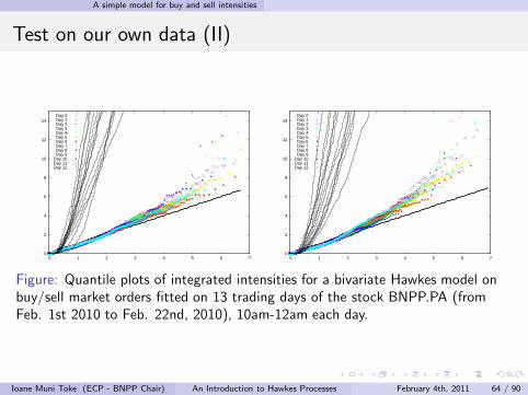
Figure: Quantile plots of integrated intensities for a bivariate Hawkes model onbuy/sell market orders fitted on 13 trading days of the stock BNPP.PA (fromFeb. 1st 2010 to Feb. 22nd, 2010), 10am-12am each day.
Ioane Muni Toke (ECP - BNPP Chair) An Introduction to Hawkes Processes February 4th, 2011 64 / 90
Modelling microstructure noise
Table of contents
1 An Introduction to Point ProcessesBasic definitionsTransformation to Poisson processes
2 One-dimensional Hawkes processesDefinition and stationarity propertiesSimulation of a Hawkes processMaximum-likelihood estimation
3 Multidimensional Hawkes processesDefinition and stationarity conditionSimulation of a multivariate Hawkes processMaximum-likelihood estimation
4 A simple model for buy and sell intensities
5 Modelling microstructure noise
6 Some statistical findings about the order book
7 An order book model with Hawkes processes
Ioane Muni Toke (ECP - BNPP Chair) An Introduction to Hawkes Processes February 4th, 2011 65 / 90
Modelling microstructure noise
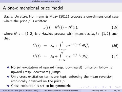
A one-dimensional price model
Bacry, Delattre, Hoffmann & Muzy (2011) propose a one-dimensional casewhere the price p is written:
p(t) = N1(t)− N2(t), (55)
where Ni , i ∈ 1, 2 is a Hawkes process with intensities λi , i ∈ 1, 2 suchthat
λ1(t) = λ0 +
∫ t
−∞
αe−β(t−s)dN2s , (56)
λ2(t) = λ0 +
∫ t
−∞
αe−β(t−s)dN1s . (57)
No self-excitation of upward (resp. downward) jumps on followingupward (resp. downward) jumps
Only cross-excitation terms are kept, enforcing the mean-reversionempirically observed on the price p
Cross-excitation is set to be symmetricIoane Muni Toke (ECP - BNPP Chair) An Introduction to Hawkes Processes February 4th, 2011 66 / 90
Modelling microstructure noise
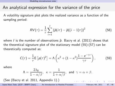
An analytical expression for the variance of the price
A volatility signature plot plots the realized variance as a function of thesampling period:
RV (τ) =1
τ
I∑
i=1
(p(iτ)− p((i − 1)τ))2 (58)
where I is the number of observations p. Bacry et al. (2011) shows thatthe theoretical signature plot of the stationary model (55)-(57) can betheoretically computed as:
C (τ) =1
τE[
p(τ)2]
= Λ
(
κ2 + (1− κ2)1− e−γτ
γτ
)
, (59)
where
Λ =2λ0
1− α/β, κ =
1
1 + α/β, and γ = α+ β.
(See (Bacry et al. 2011, Appendix 1).)Ioane Muni Toke (ECP - BNPP Chair) An Introduction to Hawkes Processes February 4th, 2011 67 / 90
Modelling microstructure noise
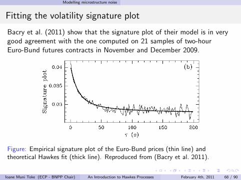
Fitting the volatility signature plot
Bacry et al. (2011) show that the signature plot of their model is in verygood agreement with the one computed on 21 samples of two-hourEuro-Bund futures contracts in November and December 2009.
Figure: Empirical signature plot of the Euro-Bund prices (thin line) andtheoretical Hawkes fit (thick line). Reproduced from (Bacry et al. 2011).
Ioane Muni Toke (ECP - BNPP Chair) An Introduction to Hawkes Processes February 4th, 2011 68 / 90
Modelling microstructure noise
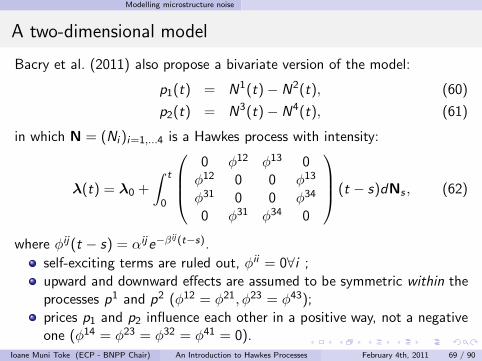
A two-dimensional model
Bacry et al. (2011) also propose a bivariate version of the model:
p1(t) = N1(t)− N2(t), (60)
p2(t) = N3(t)− N4(t), (61)
in which N = (Ni )i=1,...4 is a Hawkes process with intensity:
λ(t) = λ0 +
∫ t
0
0 φ12 φ13 0φ12 0 0 φ13
φ31 0 0 φ34
0 φ31 φ34 0
(t − s)dNs , (62)
where φij(t − s) = αije−βij (t−s).
self-exciting terms are ruled out, φii = 0∀i ;upward and downward effects are assumed to be symmetric within theprocesses p1 and p2 (φ12 = φ21, φ23 = φ43);
prices p1 and p2 influence each other in a positive way, not a negativeone (φ14 = φ23 = φ32 = φ41 = 0).
Ioane Muni Toke (ECP - BNPP Chair) An Introduction to Hawkes Processes February 4th, 2011 69 / 90
Modelling microstructure noise
An explicit expression for the covariance matrix
For this model, Bacry et al. (2011) show that an explicit form of thecorrelation coefficient
ρ(τ) = Corr (p1(t + τ)− p1(t), p2(t + τ)− p2(t)) (63)
can be explicitly computed, although the expected result is quitecumbersome (see (Bacry et al. 2011, Proposition 3.1)).
Ioane Muni Toke (ECP - BNPP Chair) An Introduction to Hawkes Processes February 4th, 2011 70 / 90
Modelling microstructure noise
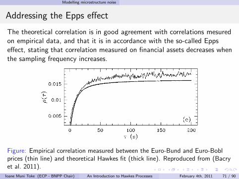
Addressing the Epps effect
The theoretical correlation is in good agreement with correlations mesuredon empirical data, and that it is in accordance with the so-called Eppseffect, stating that correlation measured on financial assets decreases whenthe sampling frequency increases.
Figure: Empirical correlation measured between the Euro-Bund and Euro-Boblprices (thin line) and theoretical Hawkes fit (thick line). Reproduced from (Bacryet al. 2011).
Ioane Muni Toke (ECP - BNPP Chair) An Introduction to Hawkes Processes February 4th, 2011 71 / 90
Some statistical findings about the order book
Table of contents
1 An Introduction to Point ProcessesBasic definitionsTransformation to Poisson processes
2 One-dimensional Hawkes processesDefinition and stationarity propertiesSimulation of a Hawkes processMaximum-likelihood estimation
3 Multidimensional Hawkes processesDefinition and stationarity conditionSimulation of a multivariate Hawkes processMaximum-likelihood estimation
4 A simple model for buy and sell intensities
5 Modelling microstructure noise
6 Some statistical findings about the order book
7 An order book model with Hawkes processes
Ioane Muni Toke (ECP - BNPP Chair) An Introduction to Hawkes Processes February 4th, 2011 72 / 90
Some statistical findings about the order book
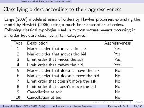
Classifying orders according to their aggressiveness
Large (2007) models streams of orders by Hawkes processes, extending themodel by Hewlett (2006) using a much finer description of orders.Following classical typologies used in microstructure, events occurring inan order book are classified in ten categories :
Type Description Aggressiveness
1 Market order that moves the ask Yes2 Market order that moves the bid Yes3 Limit order that moves the ask Yes4 Limit order that moves the bid Yes
5 Market order that doesn’t move the ask No6 Market order that doesn’t move the bid No7 Limit order that doesn’t move the ask No8 Limit order that doesn’t move the bid No9 Cancellation at ask No10 Cancellation at bid No
Ioane Muni Toke (ECP - BNPP Chair) An Introduction to Hawkes Processes February 4th, 2011 73 / 90
Some statistical findings about the order book
A 10-variate Hawkes model for aggressive orders
Events of type 1 to 4 are Hawkes processes whose intensities depend onthe 10 different sorts of events, i.e. can be written for m = 1, . . . , 4:
λm(t) = λ0(t) +
10∑
n=1
∫ t
0αmne−βmn(t−u)dNn
u . (64)
Ioane Muni Toke (ECP - BNPP Chair) An Introduction to Hawkes Processes February 4th, 2011 74 / 90
Some statistical findings about the order book
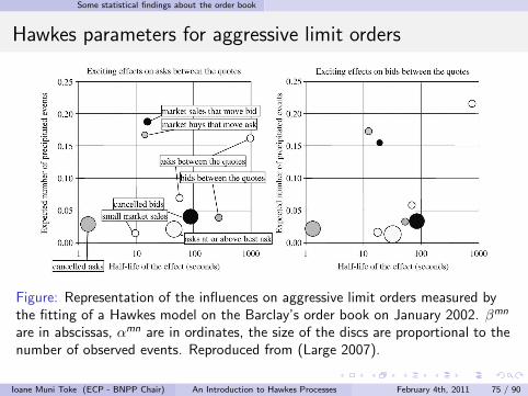
Hawkes parameters for aggressive limit orders
Figure: Representation of the influences on aggressive limit orders measured bythe fitting of a Hawkes model on the Barclay’s order book on January 2002. βmn
are in abscissas, αmn are in ordinates, the size of the discs are proportional to thenumber of observed events. Reproduced from (Large 2007).
Ioane Muni Toke (ECP - BNPP Chair) An Introduction to Hawkes Processes February 4th, 2011 75 / 90
Some statistical findings about the order book
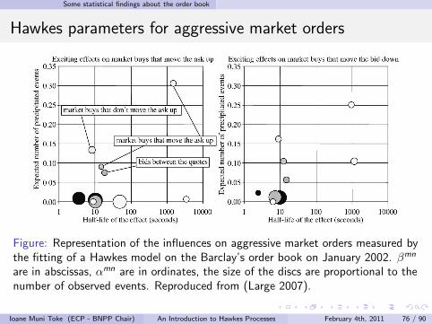
Hawkes parameters for aggressive market orders
Figure: Representation of the influences on aggressive market orders measured bythe fitting of a Hawkes model on the Barclay’s order book on January 2002. βmn
are in abscissas, αmn are in ordinates, the size of the discs are proportional to thenumber of observed events. Reproduced from (Large 2007).
Ioane Muni Toke (ECP - BNPP Chair) An Introduction to Hawkes Processes February 4th, 2011 76 / 90
Some statistical findings about the order book
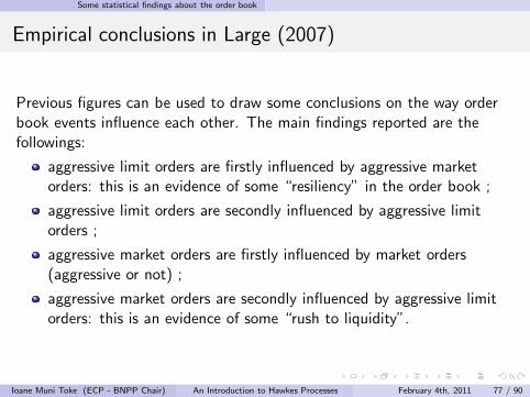
Empirical conclusions in Large (2007)
Previous figures can be used to draw some conclusions on the way orderbook events influence each other. The main findings reported are thefollowings:
aggressive limit orders are firstly influenced by aggressive marketorders: this is an evidence of some “resiliency” in the order book ;
aggressive limit orders are secondly influenced by aggressive limitorders ;
aggressive market orders are firstly influenced by market orders(aggressive or not) ;
aggressive market orders are secondly influenced by aggressive limitorders: this is an evidence of some “rush to liquidity”.
Ioane Muni Toke (ECP - BNPP Chair) An Introduction to Hawkes Processes February 4th, 2011 77 / 90
An order book model with Hawkes processes
Table of contents
1 An Introduction to Point ProcessesBasic definitionsTransformation to Poisson processes
2 One-dimensional Hawkes processesDefinition and stationarity propertiesSimulation of a Hawkes processMaximum-likelihood estimation
3 Multidimensional Hawkes processesDefinition and stationarity conditionSimulation of a multivariate Hawkes processMaximum-likelihood estimation
4 A simple model for buy and sell intensities
5 Modelling microstructure noise
6 Some statistical findings about the order book
7 An order book model with Hawkes processes
Ioane Muni Toke (ECP - BNPP Chair) An Introduction to Hawkes Processes February 4th, 2011 78 / 90
An order book model with Hawkes processes
The basic Zero-Intelligence Poisson model (“HP”)
Liquidity provider
1 arrival of new limit orders: homogeneous Poisson process NL(λL)
2 arrival of cancelation of orders: homogeneous Poisson processNC (λC )
3 new limit orders’ placement: Student’s distribution with parameters(νP1 ,m
P1 , s
P1 ) around the same side best quote
4 volume of new limit orders: exponential distribution E(1/mV1 );
5 in case of a cancelation, orders are deleted with probability δ
Noise trader (liquidity taker)
1 arrival of market orders: homogeneous Poisson process NM(µ)
2 volume of market orders: exponential distribution with meanE(1/mV
2 ).
Ioane Muni Toke (ECP - BNPP Chair) An Introduction to Hawkes Processes February 4th, 2011 79 / 90
An order book model with Hawkes processes
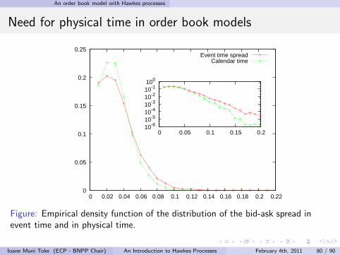
Need for physical time in order book models
0
0.05
0.1
0.15
0.2
0.25
0 0.02 0.04 0.06 0.08 0.1 0.12 0.14 0.16 0.18 0.2 0.22
Event time spreadCalendar time
10-610-510-410-310-210-1100
0 0.05 0.1 0.15 0.2
Figure: Empirical density function of the distribution of the bid-ask spread inevent time and in physical time.
Ioane Muni Toke (ECP - BNPP Chair) An Introduction to Hawkes Processes February 4th, 2011 80 / 90
An order book model with Hawkes processes
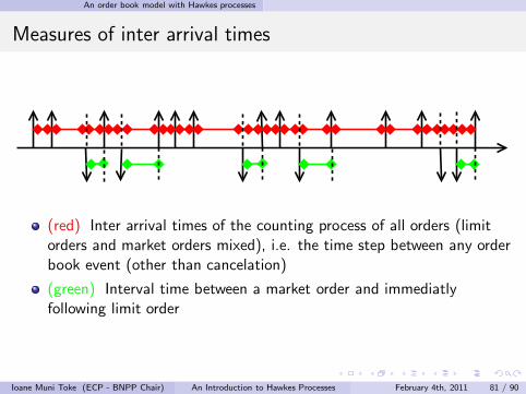
Measures of inter arrival times
(red) Inter arrival times of the counting process of all orders (limitorders and market orders mixed), i.e. the time step between any orderbook event (other than cancelation)
(green) Interval time between a market order and immediatlyfollowing limit order
Ioane Muni Toke (ECP - BNPP Chair) An Introduction to Hawkes Processes February 4th, 2011 81 / 90
An order book model with Hawkes processes
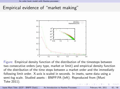
Empirical evidence of “market making”
0
0.1
0.2
0.3
0.4
0.5
0.6
0 0.1 0.2 0.3 0.4 0.5
AllOrdersMarketNextLimit
10-4
10-3
10-2
10-1
100
0.01 0.1 1 10
Figure: Empirical density function of the distribution of the timesteps betweentwo consecutive orders (any type, market or limit) and empirical density functionof the distribution of the time steps between a market order and the immediatlyfollowing limit order. X-axis is scaled in seconds. In insets, same data using asemi-log scale. Studied assets : BNPP.PA (left). Reproduced from (MuniToke 2011).
Ioane Muni Toke (ECP - BNPP Chair) An Introduction to Hawkes Processes February 4th, 2011 82 / 90
An order book model with Hawkes processes
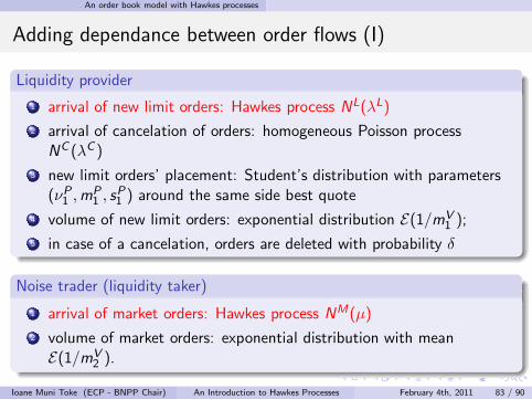
Adding dependance between order flows (I)
Liquidity provider
1 arrival of new limit orders: Hawkes process NL(λL)
2 arrival of cancelation of orders: homogeneous Poisson processNC (λC )
3 new limit orders’ placement: Student’s distribution with parameters(νP1 ,m
P1 , s
P1 ) around the same side best quote
4 volume of new limit orders: exponential distribution E(1/mV1 );
5 in case of a cancelation, orders are deleted with probability δ
Noise trader (liquidity taker)
1 arrival of market orders: Hawkes process NM(µ)
2 volume of market orders: exponential distribution with meanE(1/mV
2 ).
Ioane Muni Toke (ECP - BNPP Chair) An Introduction to Hawkes Processes February 4th, 2011 83 / 90
An order book model with Hawkes processes
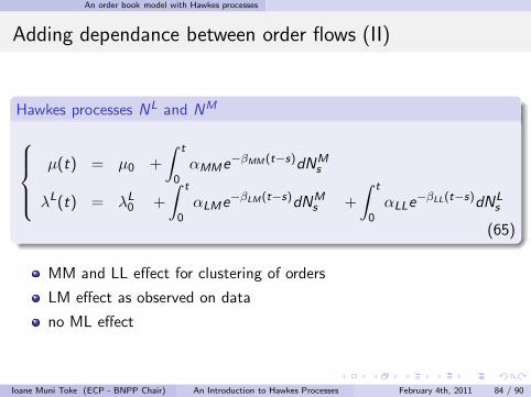
Adding dependance between order flows (II)
Hawkes processes NL and NM
µ(t) = µ0 +
∫ t
0αMMe−βMM (t−s)dNM
s
λL(t) = λL0 +
∫ t
0αLMe−βLM(t−s)dNM
s +
∫ t
0αLLe
−βLL(t−s)dNLs
(65)
MM and LL effect for clustering of orders
LM effect as observed on data
no ML effect
Ioane Muni Toke (ECP - BNPP Chair) An Introduction to Hawkes Processes February 4th, 2011 84 / 90
An order book model with Hawkes processes
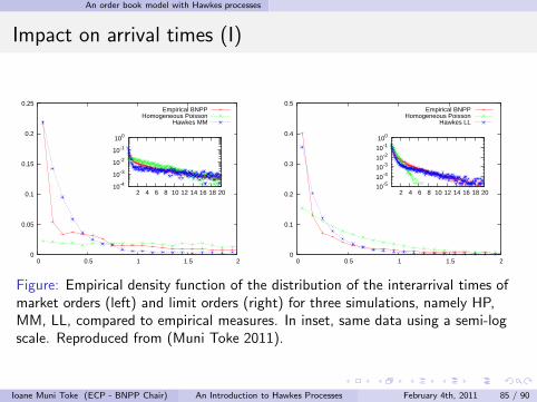
Impact on arrival times (I)
0
0.05
0.1
0.15
0.2
0.25
0 0.5 1 1.5 2
Empirical BNPPHomogeneous Poisson
Hawkes MM
10-4
10-3
10-2
10-1
100
2 4 6 8 10 12 14 16 18 20
0
0.1
0.2
0.3
0.4
0.5
0 0.5 1 1.5 2
Empirical BNPPHomogeneous Poisson
Hawkes LL
10-510-410-310-210-1100
2 4 6 8 10 12 14 16 18 20
Figure: Empirical density function of the distribution of the interarrival times ofmarket orders (left) and limit orders (right) for three simulations, namely HP,MM, LL, compared to empirical measures. In inset, same data using a semi-logscale. Reproduced from (Muni Toke 2011).
Ioane Muni Toke (ECP - BNPP Chair) An Introduction to Hawkes Processes February 4th, 2011 85 / 90
An order book model with Hawkes processes
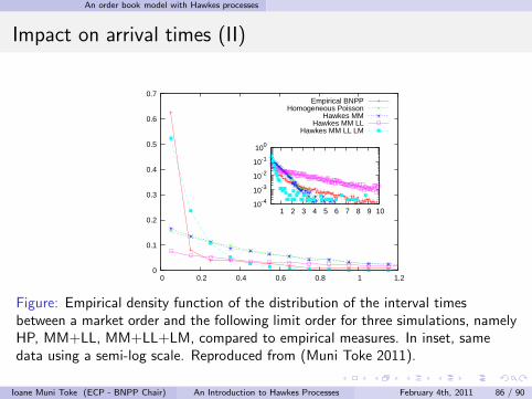
Impact on arrival times (II)
0
0.1
0.2
0.3
0.4
0.5
0.6
0.7
0 0.2 0.4 0.6 0.8 1 1.2
Empirical BNPPHomogeneous Poisson
Hawkes MMHawkes MM LL
Hawkes MM LL LM
10-4
10-3
10-2
10-1
100
1 2 3 4 5 6 7 8 9 10
Figure: Empirical density function of the distribution of the interval timesbetween a market order and the following limit order for three simulations, namelyHP, MM+LL, MM+LL+LM, compared to empirical measures. In inset, samedata using a semi-log scale. Reproduced from (Muni Toke 2011).
Ioane Muni Toke (ECP - BNPP Chair) An Introduction to Hawkes Processes February 4th, 2011 86 / 90
An order book model with Hawkes processes
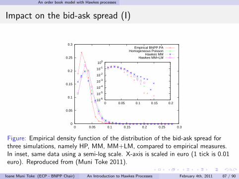
Impact on the bid-ask spread (I)
0
0.05
0.1
0.15
0.2
0.25
0.3
0 0.05 0.1 0.15 0.2 0.25 0.3
Empirical BNPP.PAHomogeneous Poisson
Hawkes MMHawkes MM+LM
10-6
10-5
10-4
10-3
10-2
10-1
100
0 0.05 0.1 0.15 0.2
Figure: Empirical density function of the distribution of the bid-ask spread forthree simulations, namely HP, MM, MM+LM, compared to empirical measures.In inset, same data using a semi-log scale. X-axis is scaled in euro (1 tick is 0.01euro). Reproduced from (Muni Toke 2011).
Ioane Muni Toke (ECP - BNPP Chair) An Introduction to Hawkes Processes February 4th, 2011 87 / 90
An order book model with Hawkes processes
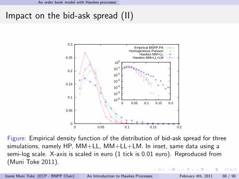
Impact on the bid-ask spread (II)
0
0.05
0.1
0.15
0.2
0.25
0.3
0 0.05 0.1 0.15 0.2
Empirical BNPP.PAHomogeneous Poisson
Hawkes MM+LLHawkes MM+LL+LM
10-6
10-5
10-4
10-3
10-2
10-1
100
0 0.05 0.1 0.15 0.2
Figure: Empirical density function of the distribution of bid-ask spread for threesimulations, namely HP, MM+LL, MM+LL+LM. In inset, same data using asemi-log scale. X-axis is scaled in euro (1 tick is 0.01 euro). Reproduced from(Muni Toke 2011).
Ioane Muni Toke (ECP - BNPP Chair) An Introduction to Hawkes Processes February 4th, 2011 88 / 90
An order book model with Hawkes processes
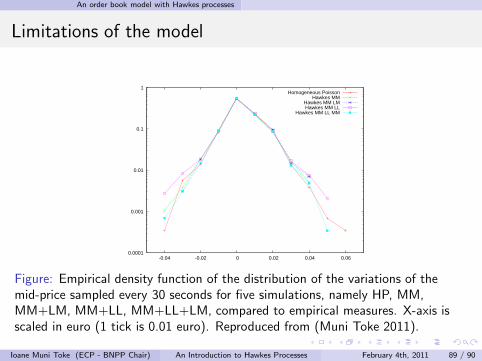
Limitations of the model
0.0001
0.001
0.01
0.1
1
-0.04 -0.02 0 0.02 0.04 0.06
Homogeneous PoissonHawkes MM
Hawkes MM LMHawkes MM LL
Hawkes MM LL MM
Figure: Empirical density function of the distribution of the variations of themid-price sampled every 30 seconds for five simulations, namely HP, MM,MM+LM, MM+LL, MM+LL+LM, compared to empirical measures. X-axis isscaled in euro (1 tick is 0.01 euro). Reproduced from (Muni Toke 2011).
Ioane Muni Toke (ECP - BNPP Chair) An Introduction to Hawkes Processes February 4th, 2011 89 / 90
Conclusion
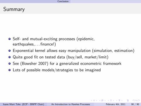
Summary
Self- and mutual-exciting processes (epidemic,earthquakes,. . . finance!)
Exponential kernel allows easy manipulation (simulation, estimation)
Quite good fit on tested data (buy/sell, market/limit)
See (Bowsher 2007) for a generalized econometric framework
Lots of possible models/strategies to be imagined
Ioane Muni Toke (ECP - BNPP Chair) An Introduction to Hawkes Processes February 4th, 2011 90 / 90
References
Bacry, E., Delattre, S., Hoffmann, M. & Muzy, J. F. (2011), ‘Modelingmicrostructure noise with mutually exciting point processes’,arXiv:1101.3422v1 .
Bowsher, C. G. (2007), ‘Modelling security market events in continuoustime: Intensity based, multivariate point process models’, Journal ofEconometrics 141(2), 876–912.
Hawkes, A. G. (1971), ‘Spectra of some self-exciting and mutually excitingpoint processes’, Biometrika 58(1), 83 –90.
Hewlett, P. (2006), Clustering of order arrivals, price impact and tradepath optimisation, in ‘Workshop on Financial Modeling with Jumpprocesses, Ecole Polytechnique’.
Large, J. (2007), ‘Measuring the resiliency of an electronic limit orderbook’, Journal of Financial Markets 10(1), 1–25.
Lewis, P. A. W. & Shedler, G. S. (1979), ‘Simulation of nonhomogeneouspoisson processes by thinning’, Naval Research Logistics Quarterly
26(3), 403–413.Muni Toke, I. (2011), ”Market making” in an order book model and its
impact on the bid-ask spread, in F. Abergel, B. Chakrabarti,
Ioane Muni Toke (ECP - BNPP Chair) An Introduction to Hawkes Processes February 4th, 2011 90 / 90
References
A. Chakraborti & M. Mitra, eds, ‘Econophysics of Order-DrivenMarkets’, New Economic Windows, Springer-Verlag Milan, pp. 49–64.
Ogata, Y. (1978), ‘The asymptotic behaviour of maximum likelihoodestimators for stationary point processes’, Annals of the Institute of
Statistical Mathematics 30(1), 243–261.Ogata, Y. (1981), ‘On Lewis’ simulation method for point processes’,
IEEE Transactions on Information Theory 27(1), 23–31.
Ioane Muni Toke (ECP - BNPP Chair) An Introduction to Hawkes Processes February 4th, 2011 90 / 90
Recommended


![arXiv:0909.1974v1 [q-fin.GN] 10 Sep 2009€¦ · arXiv:0909.1974v1 [q-fin.GN] 10 Sep 2009 Econophysics: Empirical facts and agent-based models Anirban Chakrabortia, Ioane Muni Tokea,](https://img.pdfslide.us/doc/110x75/5f0ff0377e708231d446a2a8/arxiv09091974v1-q-fingn-10-sep-arxiv09091974v1-q-fingn-10-sep-2009-econophysics.jpg)