
Naval Research LaboratoryStennis Space Center, MS 39529-5004
NRL/MR/7440--08-9126
Approved for public release; distribution is unlimited.
An Interactive Parallel CoordinatesTechnique Applied to a TropicalCyclone Climate AnalysisChad a. Steed
Mapping, Charting, and Geodesy Branch Marine Geosciences Division
PatriCk J. FitzPatriCk
Northern Gulf Institute, Mississippi State University Stennis Space Center, Mississippi
June 6, 2008
t.J. Jankun-kelly J. edward Swan iiDepartment of Computer Science Mississippi State University, Mississippi
amber n. yanCey
Department of Physics and Astronomy Mississippi State University, Mississippi
i
REPORT DOCUMENTATION PAGE Form ApprovedOMB No. 0704-0188
3. DATES COVERED (From - To)
Standard Form 298 (Rev. 8-98)Prescribed by ANSI Std. Z39.18
Public reporting burden for this collection of information is estimated to average 1 hour per response, including the time for reviewing instructions, searching existing data sources, gathering and maintaining the data needed, and completing and reviewing this collection of information. Send comments regarding this burden estimate or any other aspect of this collection of information, including suggestions for reducing this burden to Department of Defense, Washington Headquarters Services, Directorate for Information Operations and Reports (0704-0188), 1215 Jefferson Davis Highway, Suite 1204, Arlington, VA 22202-4302. Respondents should be aware that notwithstanding any other provision of law, no person shall be subject to any penalty for failing to comply with a collection of information if it does not display a currently valid OMB control number. PLEASE DO NOT RETURN YOUR FORM TO THE ABOVE ADDRESS.
5a. CONTRACT NUMBER
5b. GRANT NUMBER
5c. PROGRAM ELEMENT NUMBER
5d. PROJECT NUMBER
5e. TASK NUMBER
5f. WORK UNIT NUMBER
2. REPORT TYPE1. REPORT DATE (DD-MM-YYYY)
4. TITLE AND SUBTITLE
6. AUTHOR(S)
8. PERFORMING ORGANIZATION REPORT NUMBER
7. PERFORMING ORGANIZATION NAME(S) AND ADDRESS(ES)
10. SPONSOR / MONITOR’S ACRONYM(S)9. SPONSORING / MONITORING AGENCY NAME(S) AND ADDRESS(ES)
11. SPONSOR / MONITOR’S REPORT NUMBER(S)
12. DISTRIBUTION / AVAILABILITY STATEMENT
13. SUPPLEMENTARY NOTES
14. ABSTRACT
15. SUBJECT TERMS
16. SECURITY CLASSIFICATION OF:
a. REPORT
19a. NAME OF RESPONSIBLE PERSON
19b. TELEPHONE NUMBER (include areacode)
b. ABSTRACT c. THIS PAGE
18. NUMBEROF PAGES
17. LIMITATIONOF ABSTRACT
An Interactive Parallel Coordinates TechniqueApplied to a Tropical Cyclone Climate Analysis
Chad A. Steed, Patrick J. Fitzpatrick, T.J. Jankun-Kelly,Amber N. Yancey, and J. Edward Swan II
Naval Research LaboratoryMarine Geosciences DivisionStennis Space Center, MS 39529-5004 NRL/MR/7440--06-9126
Approved for public release; distribution is unlimited.
Unclassified Unclassified UnclassifiedUL 28
Chad Steed
(228) 688-4558
Parallel coordinatesExploratory data analysis
An enhanced interactive variant of the parallel coordinates visualization technique is presented. An example of its capabilities is demonstrated on a hurricane climate dataset. Its capabilities include focus+context filtering, dynamic visual queries with sliders, statistical displays, relocatable axes, axis inversion, details-on-demand, a pop-up menu interface, and aerial perspective shading. Furthermore, parallel coordinates can visually depict the same correlations that weather scientists find meaningful. It is demonstrated that these interactive parallel coordinates enhancements provide a deeper understanding when used in conjunction with traditional multiple regression analysis.
06-06-2008 Memorandum Report
Office of Naval ResearchOne Liberty Center875 North Randolph St.Arlington, VA 22203-1995
74-9531-08
ONR
HurricaneClimate study

CONTENTS
1 Introduction ............................................................................................................................................. 1
2 Related Work ........................................................................................................................................... 3
3 Climate Study Dataset ............................................................................................................................. 4
4 A Dynamic Interactive Parallel Coordinates Application ....................................................................... 8
5 Parallel Coordinates Validation: North Atlantic Case Study .................................................................. 13
6 Conclusion .............................................................................................................................................. 23
Acknowledgements ..................................................................................................................................... 23
References ................................................................................................................................................... 23
iii
1 Introduction
In climate studies, scientists are interested in discovering which environmentalfactors influence significant weather phenomena. A prominent weather featureis a tropical cyclone, defined as a warm-core non-frontal synoptic-scale cyclone,originating over tropical or subtropical waters, with organized thunderstormsand a closed surface wind circulation. Tropical cyclones begin as a tropicaldepression, with sustained 10-meter winds less than 17 ms−1. Most intensifyinto tropical storms (sustained winds between 17 and 32 ms−1). 56% of tropicalcyclones reach winds of at least 33 ms−1, and are then designated with regionalterms such as hurricanes in the Atlantic basin, and typhoons in the WesternNorth Pacific Ocean. When sustained 10-meter winds reach 49 ms−1, they arecalled intense hurricanes in the Atlantic.
Tropical cyclone activity in each ocean basin can vary on a yearly scale as wellas a multidecadal scale due to large-scale atmospheric influences and climateforcing. As a result, scientists are developing procedures to forecast whetheran upcoming tropical cyclone season will be active, normal, or below normal.Others are studying causes of multidecadal cycles, and whether anthropogenicglobal warming is also an influence (Landsea, 2005). Recent destructive trop-ical cyclones seasons have escalated these research efforts.
Several atmospheric and climate variables impact the intensity and frequencyof seasonal storm activity. Identifying the most critical environmental vari-ables help scientists generate more accurate seasonal forecasts which, in turn,improve the preparedness of the general public and emergency agencies. Oneuseful method for predicting and understanding the seasonal variability intropical cyclones is multiple regression. Predictors are chosen from historicaltropical cyclone data (Vitart, 2004), and provide an ordered list of the mostimportant predictors for the dynamic parameters.
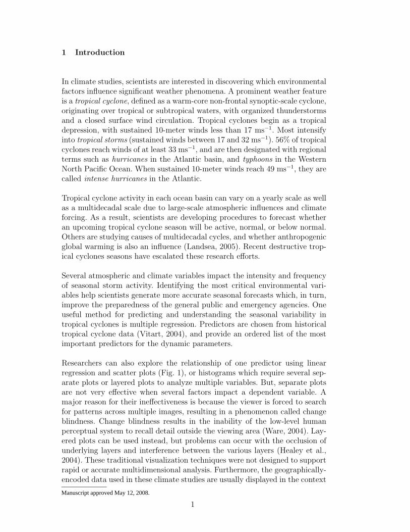
Researchers can also explore the relationship of one predictor using linearregression and scatter plots (Fig. 1), or histograms which require several sep-arate plots or layered plots to analyze multiple variables. But, separate plotsare not very effective when several factors impact a dependent variable. Amajor reason for their ineffectiveness is because the viewer is forced to searchfor patterns across multiple images, resulting in a phenomenon called changeblindness. Change blindness results in the inability of the low-level humanperceptual system to recall detail outside the viewing area (Ware, 2004). Lay-ered plots can be used instead, but problems can occur with the occlusion ofunderlying layers and interference between the various layers (Healey et al.,2004). These traditional visualization techniques were not designed to supportrapid or accurate multidimensional analysis. Furthermore, the geographically-encoded data used in these climate studies are usually displayed in the context
1
_______________Manuscript approved May 12, 2008.
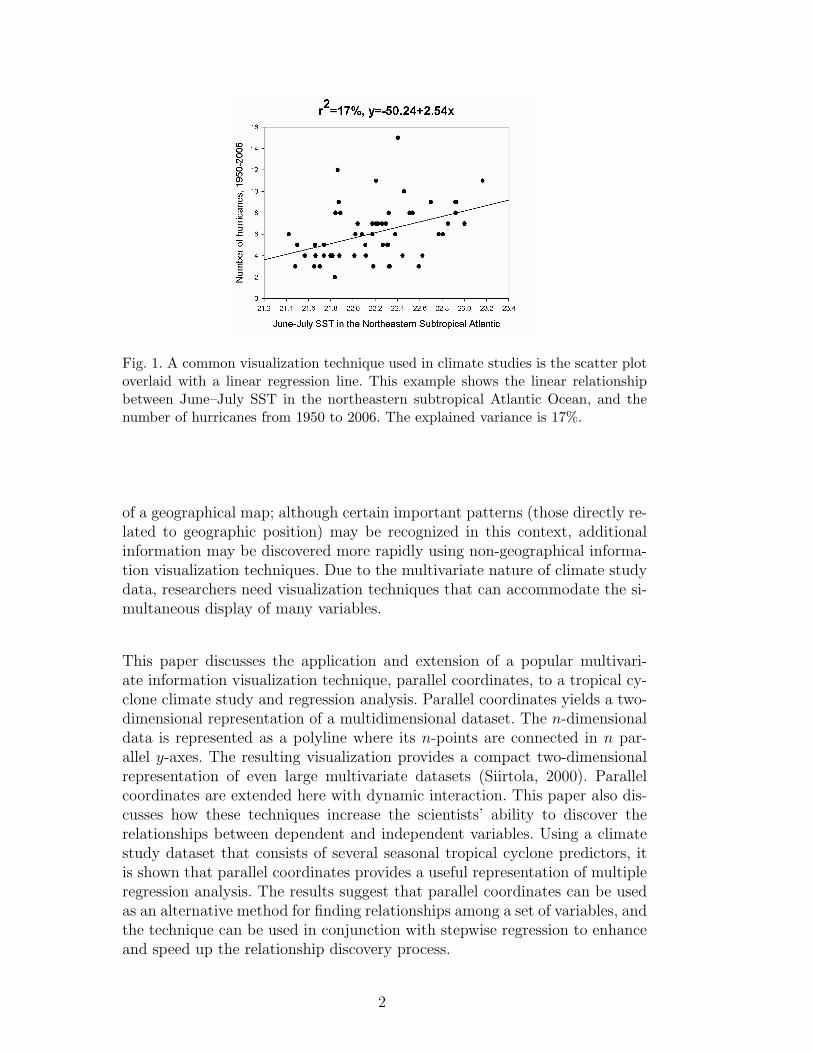
Fig. 1. A common visualization technique used in climate studies is the scatter plotoverlaid with a linear regression line. This example shows the linear relationshipbetween June–July SST in the northeastern subtropical Atlantic Ocean, and thenumber of hurricanes from 1950 to 2006. The explained variance is 17%.
of a geographical map; although certain important patterns (those directly re-lated to geographic position) may be recognized in this context, additionalinformation may be discovered more rapidly using non-geographical informa-tion visualization techniques. Due to the multivariate nature of climate studydata, researchers need visualization techniques that can accommodate the si-multaneous display of many variables.
This paper discusses the application and extension of a popular multivari-ate information visualization technique, parallel coordinates, to a tropical cy-clone climate study and regression analysis. Parallel coordinates yields a two-dimensional representation of a multidimensional dataset. The n-dimensionaldata is represented as a polyline where its n-points are connected in n par-allel y-axes. The resulting visualization provides a compact two-dimensionalrepresentation of even large multivariate datasets (Siirtola, 2000). Parallelcoordinates are extended here with dynamic interaction. This paper also dis-cusses how these techniques increase the scientists’ ability to discover therelationships between dependent and independent variables. Using a climatestudy dataset that consists of several seasonal tropical cyclone predictors, itis shown that parallel coordinates provides a useful representation of multipleregression analysis. The results suggest that parallel coordinates can be usedas an alternative method for finding relationships among a set of variables, andthe technique can be used in conjunction with stepwise regression to enhanceand speed up the relationship discovery process.
2
Table 1New interaction and representation features added to the parallel coordinates visu-alization technique.
Focus+Context Interactively scales an axis and zooms
into a subset of relations for that axis.
Aerial Perspective Facilitates visual queries by shading lines
based on proximity to the mouse cursor using a
shading scheme that mimics human perception.
Dynamic Visual Query Explores multidimensional relationships
with double-sided sliders.
Statistical Indicators Indicates statistical
quantities to support interaction model.
Relocatable Axes Reorganizes the axes by dragging with
the mouse to observe the correlation between
variables.
Axis inversion Inverts the axis display scale by swapping
the top and bottom values.
Details-on-demand Shows additional details for the highlighted axis,
and displays the value on the axis scale under the
mouse by clicking on the axis with the
middle mouse button.
Customizable Display Modifies the display (statistics
display, color schemes, tick marks) via a pop-up
menu interface.
2 Related Work
The parallel coordinates visualization technique was first introduced by In-selberg (1985) to represent hyper-dimensional geometries. Later, Wegman(1990) applied the technique to the analysis of multivariate relationships indata. Since then, several innovative extensions to the technique have beendescribed in visualization research literature. Hauser et al. (2002) proposedseveral brushing extensions for parallel coordinates. The software describedin this paper implements a variant of this histogram display technique and
3
ascertains its usefulness in the statistical analysis of tropical cyclone climaterelationships. Additionally, a dynamic axis re-ordering feature, axis inversioncapability and some details-on-demand features similar to Hauser et al. (2002)have been implemented. Furthermore, some interaction capabilities of Siirtola(2000) (e.g., conjunctive queries) are added, as well as a variant of the interac-tive aerial perspective shading technique of Jankun-Kelly and Waters (2006).The aerial perspective shading used in this paper highlights user-defined re-gions in the visualization using the mouse position and query sliders. Theapplication also includes a focus+context technique for axis scaling (Novotnyand Hauser, 2006).
This new software also provides dynamic query capabilities for the axes basedon the double slider concept of Ahlberg and Shneiderman (1994). Furthermore,the axes display important frequency information between the double sliderwidgets in a manner similar to the Influence Explorer of Tweedie et al. (1996).These features are summarized in Table 1.
Multiple regression traditionally has been used to identify statistically signifi-cant variables from multivariate datasets, including tropical cyclones datasets.Klotzbach et al. (2006a) use this technique to determine the most importantvariables for predicting the frequency of tropical cyclone activity for the NorthAtlantic basin. Similarly, Fitzpatrick applied stepwise regression analysis tothe prediction of tropical cyclone intensity (Fitzpatrick, 1996, 1997). It will beshown that multiple regression and dynamic parallel coordinates can compli-ment each other, with the regression identifying the relevant associations andthe interactive software highlighting additional features of the variables.
3 Climate Study Dataset
This research analyzes a dataset containing potential environmental predic-tors for a tropical cyclone climate study. This dataset was provided by theTropical Meteorology Project at Colorado State University (P. Klotzbach,personal communication), and is used to predict the frequency of Atlantictropical cyclones for the upcoming hurricane season by categories. These cat-egories include: 1] number named storms (winds 33 ms−1 or more, at whichtropical cyclones receive a “name”); 2] number of hurricanes; and 3] number ofintense hurricanes. These variables have known relationships to Atlantic trop-ical cyclone activity. For example, the North Atlantic basin has fewer tropicalcyclones during El Nino Southern Oscillation (ENSO) years, and active sea-sons in La Nina years (Chu, 2004). Because of this relationship, scientists useENSO signals as some predictors of seasonal storm activity. Scientists at theTropical Meteorology Project issue six forecast reports based on statisticallysignificant predictors from this dataset.
4
Tab
le2.
Env
iron
men
tal
trop
ical
cycl
one
clim
ate
vari
able
sev
alua
ted
aspr
edic
tors
inth
em
ulti
ple
regr
essi
onpr
oced
ure.
Var
iable
Nam
eG
eogr
aphic
alR
egio
n
(1)
June–
July
Nin
o3
5S-5
N,
90-1
50W
(eas
tern
equat
oria
ltr
opic
alP
acifi
cO
cean
)
(2)
May
SST
5S-5
N,
90-1
50W
(eas
tern
equat
oria
ltr
opic
alP
acifi
cO
cean
)
(3)
Feb
ruar
y20
0-m
bU
5S-1
0N,
35-5
5W(e
quat
oria
lE
ast
Bra
zil)
(4)
Feb
ruar
y–M
arch
200-
mb
V35
-62.
5S,
70-9
5E(S
outh
India
nO
cean
)
(5)
Feb
ruar
ySL
P0-
45S,
90-1
80W
(eas
tern
Sou
thP
acifi
cO
cean
)
(6)
Oct
ober
–Nov
emb
erSL
P45
-60N
,12
0-16
0W(G
ulf
ofA
lask
a)
(7)
Sep
t.50
0-m
bG
eop
oten
tial
Hei
ght
35-5
5N,
100-
120W
(wes
tern
Nor
thA
mer
ica)
(8)
Nov
emb
erSL
P7.
5-22
.5N
,12
5-17
5W(s
ubtr
opic
alnor
thea
stP
acifi
cO
cean
)
(9)
Mar
ch–A
pri
lSL
P0-
20N
,0-
40W
(eas
tern
trop
ical
Atl
anti
cO
cean
)
(10)
June–
July
SL
P10
-25N
,10
-60W
(tro
pic
alA
tlan
tic
Oce
an)
(11)
Sep
tem
ber
–Nov
emb
erSL
P15
-35N
,75
-97W
(sou
thea
stG
ulf
ofM
exic
o)
(12)
Nov
.50
0-m
bG
eop
oten
tial
Hei
ght
67.5
-85N
,50
W-1
0E(N
orth
Atl
anti
cO
cean
)
(13)
July
50-m
bU
5S-5
N,
0-36
0(e
quat
oria
lgl
obe)
(14)
Feb
ruar
ySST
35-5
0N,
10-3
0W(n
orth
wes
tE
uro
pea
nC
oast
)
(15)
Apri
l–M
aySST
30-4
5N,
10-3
0W(n
orth
wes
tE
uro
pea
nC
oast
)
(16)
June–
July
SST
20-4
0N,
15-3
5W(n
orth
east
subtr
opic
alA
tlan
tic
Oce
an)
5
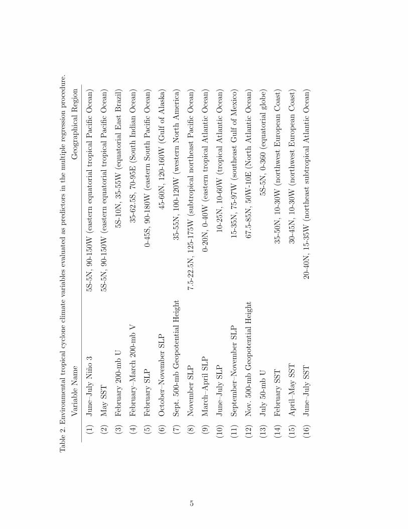
Table 2 lists 16 potential environmental predictors from the dataset alongwith their geographical region. In the remainder of this section, the physicalrelationships of these climate variables to Atlantic tropical cyclone activityare discussed.
3.1 El Nino Variables
In a normal year, air rises in the western tropical Pacific (where the wateris the warmest as well as slightly elevated) and sinks in the eastern tropicalPacific which is a phenomenon known as the Walker Circulation. During an ElNino event, the easterly surface trade winds that cause this water bulge in thewestern Pacific weaken, and the warm water travels eastward. Furthermore,El Nino conditions shift the upward portion of the Walker Circulation to theeastern Pacific, creating upper-level westerly winds in the Atlantic Ocean aswell as subsidence. Both of these factors inhibit tropical cyclone formation andintensification in this region. Opposite conditions (abnormally strong tradewinds and colder than normal eastern Pacific water) are called La Nina. LaNina years are associated with weak wind shear and little subsidence in theAtlantic, typically producing active tropical cyclone activity in this basin.
El Nino events are characterized by several possible variables. The June–JulyNino 3 (1) variable represents sea surface temperature (SST) anomalies ofthe eastern equatorial tropical Pacific Ocean. Positive values of this variableindicate an El Nino event, and negative represents a La Nina event. May SSTin the eastern equatorial Pacific (2) represents a similar relationship. The firstclues of an impending El Nino can be detected in February by observing threevariables. Upper-level westerly (zonal) wind anomalies off the northeast coastof South America imply that the upward branch of the Walker Circulationassociated with ENSO remains in the western Pacific and that El Nino con-ditions are likely to be present in the eastern equatorial Pacific for the next4-6 months. This situation is measured by the February 200-mb zonal wind(U) in equatorial East Brazil (3). Likewise, anomalous late winter meridional(north) winds at 200-mb in the South Indian Ocean are also associated with ElNino conditions (February–March 200-mb V in the South Indian Ocean (4)).Finally, sea level pressure (SLP) in the eastern Pacific south of the equator isa measure of the trade winds whereby weak trade winds (or westerly surfacewinds) are associated with lower SLP and, therefore, El Nino conditions, whilethe opposite is correlated to La Nina conditions. Therefore, February SLP inthe eastern South Pacific (5) is a possible variable. Some Fall variables are alsocorrelated to El Nino conditions, such as the October–November SLP in theGulf of Alaska (6), September 500-mb Geopotential Height in western NorthAmerica (7), and November SLP in the subtropical northeast Pacific (8).
6
3.2 Sea Level Pressure Variables
Pressure in the Atlantic Ocean is also inversely related to tropical cyclone ac-tivity, and seems to contain both monthly as well as longer term relationships.Low SLP in the tropical Atlantic implies increased atmospheric instability,moisture, and ascent (more favorable for the genesis of tropical cyclones), andweaker trade winds (which correspond to less wind shear that can tear up thethunderstorms in tropical cyclones). Low SLP in the spring tends to persistthrough the summer and fall. Therefore, potential variables include March–April SLP in the eastern tropical Atlantic (9), June–July SLP in the tropicalAtlantic (10), and September–November SLP in the southeast Gulf of Mexico(11).
3.3 Teleconnection Variables
The atmosphere is characterized by long-term oscillations which impact globalwind patterns, known as teleconnections. Two of these are the Arctic Oscil-lation and the North Atlantic Oscillation. When these oscillations are in onephase, they cause more ridges in the Atlantic, which corresponds to less windshear. Also, on decadal timescales, weaker zonal winds in the sub-polar ar-eas are indicative of a relatively strong thermohaline circulation and thereforea warmer Atlantic Ocean. A variable which measures this oscillation is theNovember 500-mb Geopotential Height in the North Atlantic (12).
3.4 Quasi-Biennial Oscillation Variable
Research has also shown that the Quasi-Biennial Oscillation (QBO) is corre-lated to tropical cyclone activity. The QBO is a stratospheric (16 to 35 kmaltitude) oscillation of equatorial east-west winds which vary with a periodof about 26 to 30 months or roughly 2 years. These winds typically blow for12-16 months from the east, then reverse and blow 12-16 months from thewest, then back to easterly again. The west phase of the QBO has been shownto provide favorable conditions for development of tropical cyclones, possiblybecause it reduces wind shear. A variable which measures the QBO is the July50-mb Equatorial Wind (U) around the globe (13).
7
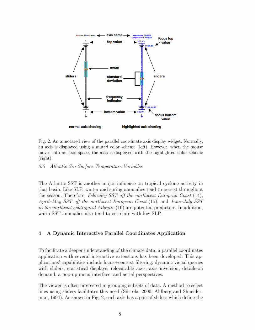
Fig. 2. An annotated view of the parallel coordinate axis display widget. Normally,an axis is displayed using a muted color scheme (left). However, when the mousemoves into an axis space, the axis is displayed with the highlighted color scheme(right).
3.5 Atlantic Sea Surface Temperature Variables
The Atlantic SST is another major influence on tropical cyclone activity inthat basin. Like SLP, winter and spring anomalies tend to persist throughoutthe season. Therefore, February SST off the northwest European Coast (14),April–May SST off the northwest European Coast (15), and June–July SSTin the northeast subtropical Atlantic (16) are potential predictors. In addition,warm SST anomalies also tend to correlate with low SLP.
4 A Dynamic Interactive Parallel Coordinates Application
To facilitate a deeper understanding of the climate data, a parallel coordinatesapplication with several interactive extensions has been developed. This ap-plications’ capabilities include focus+context filtering, dynamic visual querieswith sliders, statistical displays, relocatable axes, axis inversion, details-ondemand, a pop-up menu interface, and aerial perspectives.
The viewer is often interested in grouping subsets of data. A method to selectlines using sliders facilitates this need (Siirtola, 2000; Ahlberg and Shneider-man, 1994). As shown in Fig. 2, each axis has a pair of sliders which define the
8
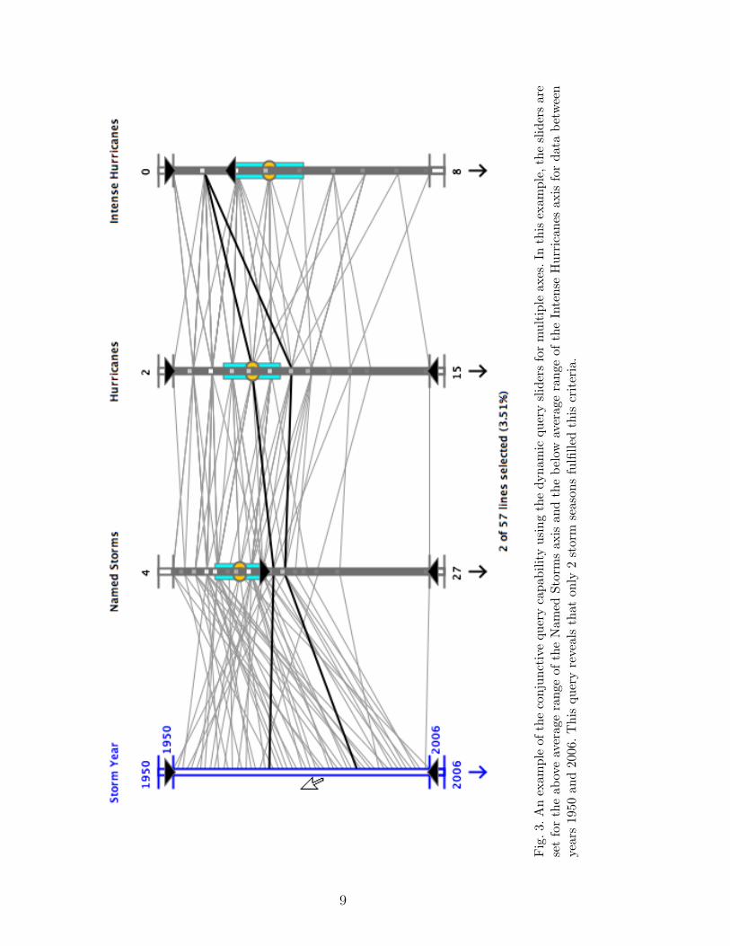
Fig
.3.A
nex
ampl
eof
the
conj
unct
ive
quer
yca
pabi
lity
usin
gth
edy
nam
icqu
ery
slid
ers
for
mul
tipl
eax
es.I
nth
isex
ampl
e,th
esl
ider
sar
ese
tfo
rth
eab
ove
aver
age
rang
eof
the
Nam
edSt
orm
sax
isan
dth
ebe
low
aver
age
rang
eof
the
Inte
nse
Hur
rica
nes
axis
for
data
betw
een
year
s19
50an
d20
06.
Thi
squ
ery
reve
als
that
only
2st
orm
seas
ons
fulfi
lled
this
crit
eria
.
9
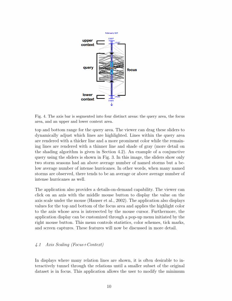
Fig. 4. The axis bar is segmented into four distinct areas: the query area, the focusarea, and an upper and lower context area.
top and bottom range for the query area. The viewer can drag these sliders todynamically adjust which lines are highlighted. Lines within the query areaare rendered with a thicker line and a more prominent color while the remain-ing lines are rendered with a thinner line and shade of gray (more detail onthe shading algorithm is given in Section 4.2). An example of a conjunctivequery using the sliders is shown in Fig. 3. In this image, the sliders show onlytwo storm seasons had an above average number of named storms but a be-low average number of intense hurricanes. In other words, when many namedstorms are observed, there tends to be an average or above average number ofintense hurricanes as well.
The application also provides a details-on-demand capability. The viewer canclick on an axis with the middle mouse button to display the value on theaxis scale under the mouse (Hauser et al., 2002). The application also displaysvalues for the top and bottom of the focus area and applies the highlight colorto the axis whose area is intersected by the mouse cursor. Furthermore, theapplication display can be customized through a pop-up menu initiated by theright mouse button. This menu controls statistics, color schemes, tick marks,and screen captures. These features will now be discussed in more detail.
4.1 Axis Scaling (Focus+Context)
In displays where many relation lines are shown, it is often desirable to in-teractively tunnel through the relations until a smaller subset of the originaldataset is in focus. This application allows the user to modify the minimum
10
(a) (b)
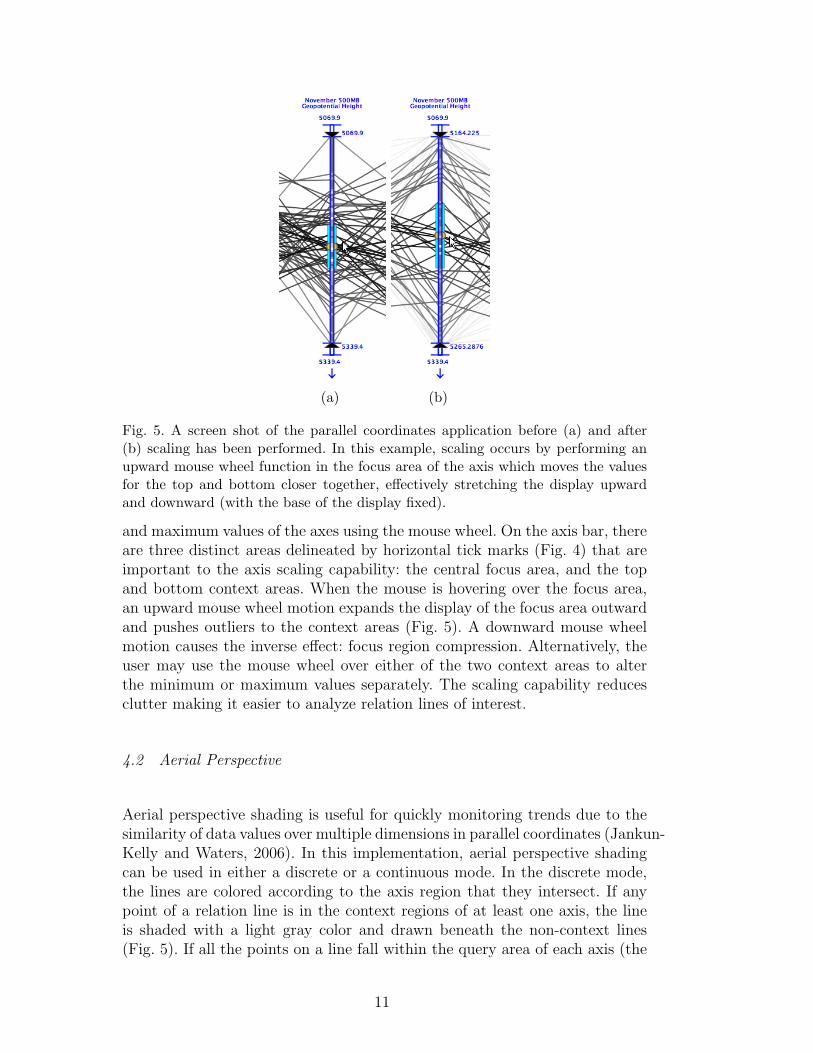
Fig. 5. A screen shot of the parallel coordinates application before (a) and after(b) scaling has been performed. In this example, scaling occurs by performing anupward mouse wheel function in the focus area of the axis which moves the valuesfor the top and bottom closer together, effectively stretching the display upwardand downward (with the base of the display fixed).
and maximum values of the axes using the mouse wheel. On the axis bar, thereare three distinct areas delineated by horizontal tick marks (Fig. 4) that areimportant to the axis scaling capability: the central focus area, and the topand bottom context areas. When the mouse is hovering over the focus area,an upward mouse wheel motion expands the display of the focus area outwardand pushes outliers to the context areas (Fig. 5). A downward mouse wheelmotion causes the inverse effect: focus region compression. Alternatively, theuser may use the mouse wheel over either of the two context areas to alterthe minimum or maximum values separately. The scaling capability reducesclutter making it easier to analyze relation lines of interest.
4.2 Aerial Perspective
Aerial perspective shading is useful for quickly monitoring trends due to thesimilarity of data values over multiple dimensions in parallel coordinates (Jankun-Kelly and Waters, 2006). In this implementation, aerial perspective shadingcan be used in either a discrete or a continuous mode. In the discrete mode,the lines are colored according to the axis region that they intersect. If anypoint of a relation line is in the context regions of at least one axis, the lineis shaded with a light gray color and drawn beneath the non-context lines(Fig. 5). If all the points on a line fall within the query area of each axis (the
11
(a) Discrete aerial perspective shading.
(b) Continuous aerial perspective shading.
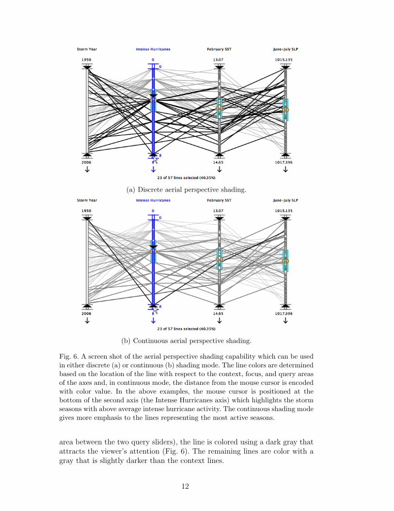
Fig. 6. A screen shot of the aerial perspective shading capability which can be usedin either discrete (a) or continuous (b) shading mode. The line colors are determinedbased on the location of the line with respect to the context, focus, and query areasof the axes and, in continuous mode, the distance from the mouse cursor is encodedwith color value. In the above examples, the mouse cursor is positioned at thebottom of the second axis (the Intense Hurricanes axis) which highlights the stormseasons with above average intense hurricane activity. The continuous shading modegives more emphasis to the lines representing the most active seasons.
area between the two query sliders), the line is colored using a dark gray thatattracts the viewer’s attention (Fig. 6). The remaining lines are color with agray that is slightly darker than the context lines.
12
In the continuous mode, non-context lines go through an additional step toencode the distance of the line from the mouse cursor. Query lines that arenearest to the mouse cursor are shaded with the darkest gray color while linesfurtherest from the mouse cursor are shaded with a lighter gray. The otherquery lines are shaded according to a non-linear fall-off function that yieldsa gradient of gray colors between extremes. Consequently, the lines that arenearest to the mouse cursor are more prominent to the viewer due to the moredrastic color contrast and depth ordering treatments (Fig. 6) giving the viewerthe ability to effectively use the mouse to perform rapid, visual queries.
4.3 Representing Key Statistics
To support the advanced interaction capabilities of this application, each axisalso shows key statistical quantities for the relation points that are displayedin the focus region (Siirtola, 2000; Hauser et al., 2002). For each axis, themean, standard deviation, and the frequency information are calculated forpoints in the focus area. As shown in Fig. 2, the mean value and the standarddeviation range are shown using two yellow half circles and two cyan rect-angles, respectively. Within each axis bar, the frequency information is alsodisplayed by representing histogram bins as small, gray rectangles with grayvalues proportional to the number of lines that pass through the bin’s region.
5 Parallel Coordinates Validation: North Atlantic Case Study
As discussed previously, regression analysis is often employed to identify themost relevant climate relationships for tropical cyclone activity. Such tech-niques are effective in screening data and providing quantitative associations.However, multivariate analysis can be difficult. This section will outline howstepwise regression and parallel coordinates can compliment each other in suchan analysis.
Stepwise regression with a “backwards glance” is used which selects the opti-mum number of most important variables using a predefined significance value(90% in this study). Stepwise regression can compliment parallel coordinatevisualization by isolating the significant variables in a quantitative fashion.An interactive parallel coordinates visualization can then be used to developa deeper understanding of the complex relationships between the variables.
An extra step is taken to ensure the proper selection of variables. The initiallychosen variables are examined for multicollinearity; if any variables are corre-lated with each other by more than 0.5, one is removed and the code rerun.
13
In this way, the chosen variables are truly independent of each other.
A normalization procedure is also done for equal comparison between the vari-ables. Denoting σ as the standard deviation of a variable, y as the dependentvariable (named storms, hurricanes, or intense hurricanes in this study), x asthe predictor mean, and y as the dependent variable mean, a number k ofstatistically significant predictors are normalized by the following regression:
(y − y)/σy =k∑
i=1
ci(xi − xi)/σi (1)
The advantage of this approach is that the importance of a predictor maybe assessed by comparing regression coefficients ci between different variables,and that the y-intercept becomes zero.
In addition, xi may be interpreted (to a first approximation) as a “threshold”value which distinguishes between positive and negative contributions (forci > 0), and the opposite for negative ci. Years when independent variablescontain large deviations from the mean could be associated with very activeor inactive years, and require closer examination. As will be seen, the parallelcoordinates technique facilitates the examination of active and quiet Atlantichurricane seasons.
The 16 potential variables listed in Table 2 are examined in the stepwise re-gression, yielding several independent variables for each dependent variable.These results show that several climate factors impact tropical cyclone activ-ity. The chosen predictors are shown in Table 3, along with their normalizedregression coefficient and sample mean. The explained variance (R2) is shownin the 3 table headings.
The stepwise regression shows only one significant El Nino variable (late win-ter South Indian Ocean 200-mb meridional winds (4)) impacts total numberof storms; it is the second most influential predictor. Late winter northwestcoastal European SST (14) is the leading predictor. The North Atlantic Oscil-lation (manifested by 500-mb geopotential height in the North Atlantic (12))ranks third, and is also the only variable seen in all three tables. This suggeststhat the presence of a ridge in the Atlantic is conducive to an above averagetropical cyclone season. Finally, low SLP in the southeast Gulf of Mexico (11)also encourages the formation of tropical cyclones. Note that the coefficienthas a negative sign, showing that the lower the pressure, the better the chanceof tropical cyclone activity.
For number of hurricanes, the analysis surprisingly shows that October–NovemberSLP in the Gulf of Alaska (6) is the most important predictor. The physicalrole is not clear, although scientists know it is correlated to El Nino activity.
14
Northeast subtropical Atlantic SST (16) and North Atlantic 500-mb geopoten-tial height (12) are tied for second, and southeast Gulf SLP again ranks fourth(11). The explained variance is 42% — more than the 34% for named storms.This suggests stronger predictor relationships for number of hurricanes.
For intense hurricanes, the variance increases to 54%. In this case, the NorthAtlantic November 500-mb height variable (12) is the strongest predictor.Early summer tropical Atlantic SLP (10) ranks number two, followed bySeptember 500-mb geopotential height in western North America (7) andFebruary SST off northwest coastal Europe (14). The higher variance and dis-tinctly different chosen predictors suggests different environmental influencesare required for intense hurricanes. This analysis correlates the presence ofhigh pressure in the western U.S. and over the Atlantic, low summer AtlanticSLP, and warm SST as necessary conditions for intense hurricanes.
Because there is unexplained variance and several predictors, can parallel co-ordinates glean any more information? To answer this question, the datasetsare stratified into below normal, normal, and above normal seasons using thesoftware’s interactive capabilities, and the significant predictors identified bythe stepwise regression are analyzed visually. Using the key statistical indi-cators, the below normal, normal, and above normal seasons are determinedby moving the query sliders for the axis of interest to encapsulate the linesabove the standard deviation range, within the standard deviation range, andbelow the standard deviation range, respectively. After setting the query slid-ers, the aerial perspective shading highlights the relationships of interest, thusenabling analysis of the variables.
Figure 7 shows a plot for seasons with below normal named storms (samplesize of 16). Even though the regression shows February Atlantic SST (14)as the most important overall predictor, it is not as effective for discerninginactive seasons. The plot shows considerable scatter, and with only 6 yearsof significantly below average SST. The dynamic query capabilities of thisparallel coordinates application make these combined queries and subsampleanalysis an intuitive exercise. September–November Gulf of Mexico SLP (11)also exhibits much scatter, with a slight majority of years with above normalpressure. However, February–March 200-mb South Indian Ocean meridionalwinds (4) — a surrogate measurement of El Nino, shows 15 seasons (94%)of strong north winds, tightly clustered in the plots. This suggests El Ninois the major contributor to inactive Atlantic tropical cyclone seasons. Notealso that below normal November North Atlantic 500-mb geopotential heights(12) plays a pivotal role for quiet seasons. Fourteen seasons (87%) containlower geopotential heights in November, suggesting the presence of upper-level troughs which can shear tropical cyclones. However, this signal is not asstrong as the El Nino predictor. Additionally, many unshaded lines exist forpositive 200-mb V, showing that other factors besides El Nino contribute to
15
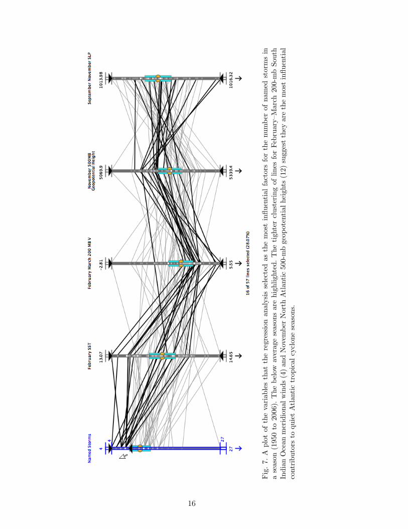
Fig
.7.
Apl
otof
the
vari
able
sth
atth
ere
gres
sion
anal
ysis
sele
cted
asth
em
ost
influ
enti
alfa
ctor
sfo
rth
enu
mbe
rof
nam
edst
orm
sin
ase
ason
(195
0to
2006
).T
hebe
low
aver
age
seas
ons
are
high
light
ed.
The
tigh
ter
clus
teri
ngof
lines
for
Febr
uary
–Mar
ch20
0-m
bSo
uth
Indi
anO
cean
mer
idio
nalw
inds
(4)
and
Nov
embe
rN
orth
Atl
anti
c50
0-m
bge
opot
enti
alhe
ight
s(1
2)su
gges
tth
eyar
eth
em
ost
influ
enti
alco
ntri
buto
rsto
quie
tA
tlan
tic
trop
ical
cycl
one
seas
ons.
16
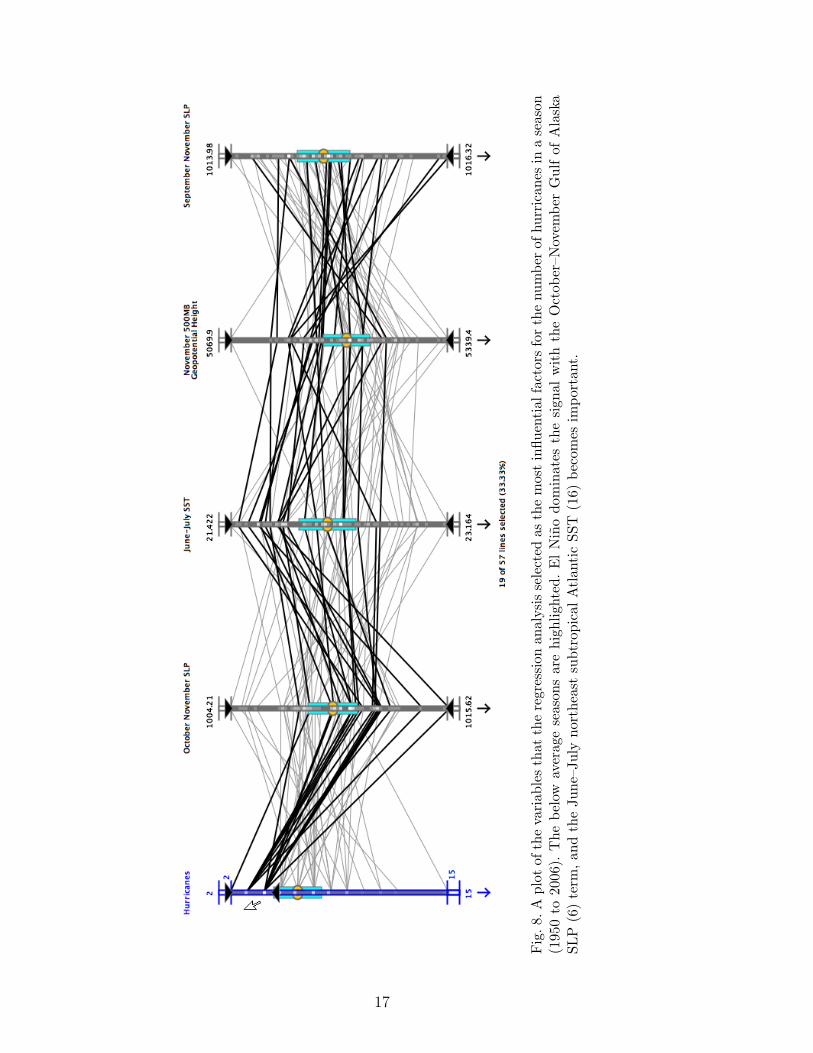
Fig
.8.A
plot
ofth
eva
riab
les
that
the
regr
essi
onan
alys
isse
lect
edas
the
mos
tin
fluen
tial
fact
ors
for
the
num
ber
ofhu
rric
anes
ina
seas
on(1
950
to20
06).
The
belo
wav
erag
ese
ason
sar
ehi
ghlig
hted
.E
lN
ino
dom
inat
esth
esi
gnal
wit
hth
eO
ctob
er–N
ovem
ber
Gul
fof
Ala
ska
SLP
(6)
term
,an
dth
eJu
ne–J
uly
nort
heas
tsu
btro
pica
lA
tlan
tic
SST
(16)
beco
mes
impo
rtan
t.
17
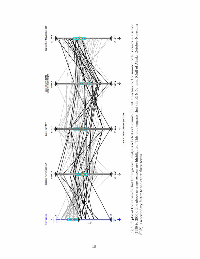
Fig
.9.A
plot
ofth
eva
riab
les
that
the
regr
essi
onan
alys
isse
lect
edas
the
mos
tin
fluen
tial
fact
ors
for
the
num
ber
ofhu
rric
anes
ina
seas
on(1
950
to20
06).
The
abov
eav
erag
ese
ason
sar
ehi
ghlig
hted
.Thi
spl
otsu
gges
tsth
atth
eE
lNin
ote
rm(G
ulf
ofA
lask
aO
ctob
er–N
ovem
ber
SLP
)is
ase
cond
ary
fact
orto
the
othe
rth
ree
term
s.
18
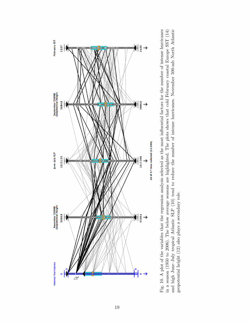
Fig
.10
.A
plot
ofth
eva
riab
les
that
the
regr
essi
onan
alys
isse
lect
edas
the
mos
tin
fluen
tial
fact
ors
for
the
num
ber
ofin
tens
ehu
rric
anes
ina
seas
on(1
950
to20
06).
The
belo
wav
erag
ese
ason
sar
ehi
ghlig
hted
.T
hepl
ots
show
sth
atco
ldFe
brua
ryco
asta
lE
urop
eSS
T(1
4)an
dhi
ghJu
ne–J
uly
trop
ical
Atl
anti
cSL
P(1
0)te
ndto
redu
ceth
enu
mbe
rof
inte
nse
hurr
ican
es.
Nov
embe
r50
0-m
bN
orth
Atl
anti
cge
opot
enti
alhe
ight
(12)
also
play
sa
seco
ndar
yro
le.
19
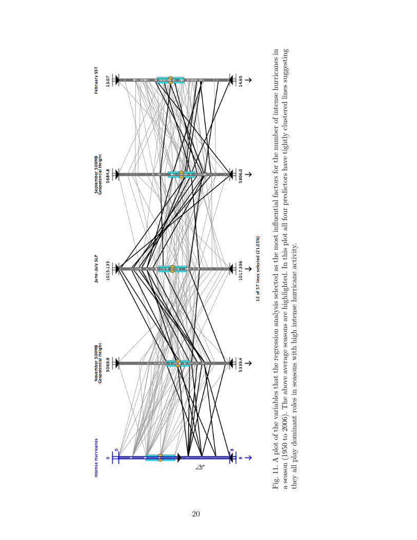
Fig
.11.
Apl
otof
the
vari
able
sth
atth
ere
gres
sion
anal
ysis
sele
cted
asth
em
ost
influ
enti
alfa
ctor
sfo
rth
enu
mbe
rof
inte
nse
hurr
ican
esin
ase
ason
(195
0to
2006
).T
heab
ove
aver
age
seas
ons
are
high
light
ed.I
nth
ispl
otal
lfou
rpr
edic
tors
have
tigh
tly
clus
tere
dlin
essu
gges
ting
they
all
play
dom
inan
tro
les
inse
ason
sw
ith
high
inte
nse
hurr
ican
eac
tivi
ty.
20
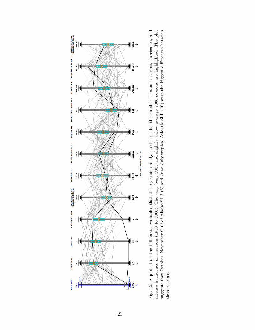
Fig
.12
.A
plot
ofal
lth
ein
fluen
tial
vari
able
sth
atth
ere
gres
sion
anal
ysis
sele
cted
for
the
num
ber
ofna
med
stor
ms,
hurr
ican
es,
and
inte
nse
hurr
ican
esin
ase
ason
(195
0to
2006
).T
heve
rybu
sy20
05an
dsl
ight
lybe
low
aver
age
2006
seas
ons
are
high
light
ed.
The
plot
sugg
ests
that
Oct
ober
–Nov
embe
rG
ulf
ofA
lask
aSL
P(6
)an
dJu
ne–J
uly
trop
ical
Atl
anti
cSL
P(1
0)w
ere
the
bigg
est
diffe
renc
esbe
twee
nth
ese
seas
ons.
21
normal and active seasons. In fact, a similar parallel coordinates stratificationanalysis shows that November North Atlantic 500-mb geopotential heights(12) and September–November Gulf of Mexico SLP (11) tend to be the criticalplayers for an active tropical cyclone season (not shown).
Figure 8 shows seasons with below normal hurricane activity (19 seasons).El Nino again tends to dominate the signal through the fall Gulf of AlaskaSLP (6) term. However, in contrast to number of named storms, AtlanticSST (16) becomes important for number of hurricanes. This suggests thatwhen water temperature is below normal, tropical storms will have difficultyreaching hurricane status. For above normal hurricane activity (Fig. 9), June–July Atlantic SST (16), November North Atlantic 500-mb geopotential height(12), and Gulf of Mexico SLP (11) tend to exert dominant roles, with El Ninoa secondary factor.
Intense hurricanes warrant special consideration, since they cause 80% of theeconomic damage from tropical cyclones. Figure 10 shows that cold FebruaryAtlantic SSTs (14) and high Atlantic June–July SLP (10) tend to reduce thenumber of intense hurricanes, with November North Atlantic 500-mb geopo-tential heights (12) playing a secondary role and September 500-mb geopo-tential heights in western North America (7) contributing no role. In contrast,all four predictors have tightly clustered lines showing they all play dominantroles in seasons with above normal intense hurricane activity (Fig. 11). Theseterms are associated with the presence of ridges in the western U.S. and theAtlantic, below average Atlantic SLP, and warm wintertime Atlantic SST offthe northwestern European Coast. Ridges are low shear environments, show-ing that the lack of upper level troughs is an important factor for seasons withmany intense hurricanes. Low SLP indicates minimal subsidence. Sinking airsuppresses cloud growth and also dries the lower atmosphere, both of whichare not conducive to the formation and development of tropical cyclones. LowSLP also could indicate better organized tropical waves (from which manyAtlantic tropical cyclones form). Warm wintertime northeast Atlantic wateralso is a good precursor for above average intense hurricane activity.
This parallel coordinates application can also investigate the differences be-tween the extremely busy 2005 season and the slightly below average 2006season. Figure 12 shows the 2005 and 2006 seasons along with the chosenpredictors from all three categories (named storms, hurricanes, and intensehurricanes) listed in Table 3. This plot reveals that most of the terms arenearly the same except for October–November SLP in the Gulf of Alaska (6)(above average in 2005, below average in 2006) and June–July SLP in the trop-ical Atlantic (10) (below average in 2005, above average in 2006). Klotzbachet al. (2006b) andBell et al. (2007) show that the tropical Atlantic was quitedry through most of the 2006 hurricane season due to subsidence associatedwith the onset of an unusually late ENSO event (indicated by the Gulf of
22
Alaska SLP), as well as frequent outbreaks of African dust storms that year.
6 Conclusion
It has been shown that parallel coordinates, a visualization technique designedspecifically for multivariate information, can be used to confirm and clarify theresults of stepwise regression when enhanced with interactive tools. The addedcapabilities discussed in this paper include focus+context filtering, dynamicvisual queries with sliders, statistical displays, relocatable axes, axis inversion,details-on demand, a pop-up menu interface, and aerial perspectives. An ap-plication to a tropical cyclone dataset shows that, while multiple regressionprovides the most significant variables, visual analysis using a dynamic paral-lel coordinates system facilitates a deeper understanding of the environmentalcauses for above average and below average hurricane seasons.
Acknowledgements
This research is sponsored by the Naval Research Laboratory’s Long-TermTraining Program, by the National Oceanographic and Atmospheric Admin-istration (NOAA) with grants NA060AR4600181 and NA050AR4601145, andthrough the Northern Gulf Institute funded by grant NA06OAR4320264. Thisparticular project was initiated in the Information Visualization course taughtat Mississippi State University by Dr. T.J. Jankun-Kelly. The authors wish tothank Dr. Phil Klotzbach of Colorado State University’s Tropical MeteorologyProject for providing the Atlantic tropical cyclone dataset.
References
Ahlberg, C., Shneiderman, B., 1994. Visual information seeking: Tight cou-pling of dynamic query filters with starfield displays. In: Proceedings ofHuman Factors in Computing Systems. ACM, Boston, MA, pp. 313–317,479–480.
Bell, G. D., Blake, E., Landsea, C. W., Chelliah, M., Pasch, R., Mo, K. C.,Goldenberg, S. B., 2007. The tropics – Atlantic basin. In: Arguez, A. (Ed.),State of the Climate in 2006. Vol. 88. Bulletin of the American Meteorolog-ical Society, pp. S48–S51.
Chu, P.-S., 2004. ENSO and tropical cyclone activity. In: Murnane, R. J.,Liu, K.-B. (Eds.), Hurricanes and Typhoons: Past, Present, and Future.Columbia University Press, pp. 297–332.
23
Fitzpatrick, P. J., 1996. Understanding and forecasting tropical cyclone inten-sity change. Ph.D. thesis, Department of Atmospheric Sciences, ColoradoState University, Fort Collins, CO.
Fitzpatrick, P. J., 1997. Understanding and forecasting tropical cyclone inten-sity change with the typhoon intensity prediction scheme (TIPS). Weatherand Forecasting 12 (4), 826–846.
Hauser, H., Ledermann, F., Doleisch, H., 2002. Angular brushing of extendedparallel coordinates. In: Proceedings of IEEE Symposium on InformationVisualization 2002. IEEE Computer Society, Boston, MA, pp. 127–130.
Healey, C. G., Tateosian, L., Enns, J. T., Remple, M., 2004. Perceptually-based brush strokes for nonphotorealistic visualization. ACM Transactionson Graphics 23 (1), 64–96.
Inselberg, A., 1985. The plane with parallel coordinates. The Visual Computer1 (4), 69–91.
Jankun-Kelly, T. J., Waters, C., 2006. Illustrative rendering for information vi-sualization. In: Posters Compendium: IEEE Visualization 2006. IEEE Com-puter Society, Baltimore, MD, pp. 42–43.
Klotzbach, P. J., Gray, W. M., Thorson, W., 2006a. Ex-tended range forecast of Atlantic seasonal hurricane activ-ity and U.S. landfall strike probability for 2007. Tech. rep.,http://tropical.atmos.colostate.edu/Forecasts/2006/dec2006/ (current25 Oct. 2007).
Klotzbach, P. J., Gray, W. M., Thorson, W., 2006b. Sum-mary of 2006 Atlantic tropical cyclone activity and verifica-tion of author’s seasonal and monthly forecasts. Tech. rep.,http://tropical.atmos.colostate.edu/Forecasts/2006/nov2006/ (current25 Oct. 2007).
Landsea, C. W., 2005. Hurricanes and global warming. EOS 438, E11–E13.Novotny, M., Hauser, H., 2006. Outlier-preserving focus+context visualization
in parallel coordinates. IEEE Transactions on Visualization and ComputerGraphics 12 (5), 893–900.
Siirtola, H., 2000. Direct manipulation of parallel coordinates. In: Proceed-ings of the International Conference on Information Visualisation. IEEEComputer Society, London, England, pp. 373–378.
Tweedie, L., Spence, R., Dawkes, H., Su, H., 1996. Externalising abstractmathematical models. In: Proceedings of the Conference on Human Factorsin Computing Systems. ACM, Vancouver, British Columbia, Canada, pp.406–412.
Vitart, F., 2004. Dynamical seasonal forecasts of tropical storm statistics. In:Murnane, R. J., Liu, K.-B. (Eds.), Hurricanes and Typhoons: Past, Present,and Future. Columbia University Press, pp. 354–392.
Ware, C., 2004. Information Visualization: Perception for Design, 2nd Edition.Morgan Kaufmann, San Francisco, CA.
Wegman, E. J., 1990. Hyperdimensional data analysis using parallel coordi-nates. Journal of the American Statistical Association 85 (411), 664–675.
24
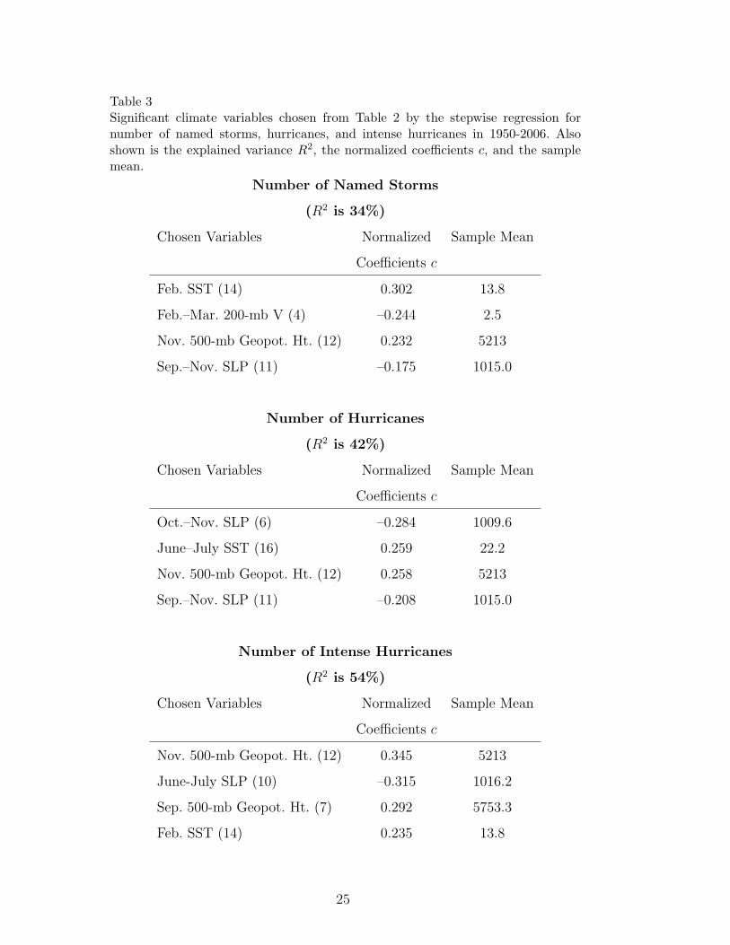
Table 3Significant climate variables chosen from Table 2 by the stepwise regression fornumber of named storms, hurricanes, and intense hurricanes in 1950-2006. Alsoshown is the explained variance R2, the normalized coefficients c, and the samplemean.
Number of Named Storms
(R2 is 34%)
Chosen Variables Normalized Sample Mean
Coefficients c
Feb. SST (14) 0.302 13.8
Feb.–Mar. 200-mb V (4) –0.244 2.5
Nov. 500-mb Geopot. Ht. (12) 0.232 5213
Sep.–Nov. SLP (11) –0.175 1015.0
Number of Hurricanes
(R2 is 42%)
Chosen Variables Normalized Sample Mean
Coefficients c
Oct.–Nov. SLP (6) –0.284 1009.6
June–July SST (16) 0.259 22.2
Nov. 500-mb Geopot. Ht. (12) 0.258 5213
Sep.–Nov. SLP (11) –0.208 1015.0
Number of Intense Hurricanes
(R2 is 54%)
Chosen Variables Normalized Sample Mean
Coefficients c
Nov. 500-mb Geopot. Ht. (12) 0.345 5213
June-July SLP (10) –0.315 1016.2
Sep. 500-mb Geopot. Ht. (7) 0.292 5753.3
Feb. SST (14) 0.235 13.8
25
Recommended


![Horse Racing Data Visualization... · 2019-12-17 · Figure 2: Variant of Sankey diagram 4.4 Parallel Coordinates The parallel coordinates [4] is a kind of multi-dimensions visual-ization](https://img.pdfslide.us/doc/110x75/5fb577632eb9ac53473ebf17/horse-racing-data-visualization-2019-12-17-figure-2-variant-of-sankey-diagram.jpg)