Download pdf - An experimental, theoretical and numerical investigation ... · In addition to experimental investigations, the ever increasing number of SMP-based applications has motivated a con-siderable

International Journal of Plasticity 67 (2015) 127–147

Contents lists available at ScienceDirect

International Journal of Plasticity

journal homepage: www.elsevier .com/locate / i jp las

An experimental, theoretical and numerical investigationof shape memory polymers

http://dx.doi.org/10.1016/j.ijplas.2014.10.0060749-6419/� 2014 Elsevier Ltd. All rights reserved.

⇑ Corresponding author. Tel.: +39 0382 985468.E-mail address: [email protected] (G. Scalet).

G. Scalet a,⇑, F. Auricchio a, E. Bonetti b, L. Castellani c, D. Ferri c, M. Pachera c, F. Scavello c

a Dipartimento di Ingegneria Civile e Architettura, Università di Pavia, Via Ferrata 3, 27100 Pavia, Italyb Dipartimento di Matematica, Università di Pavia, Via Ferrata 1, 27100 Pavia, Italyc Basic Chemicals and Plastics Research Center, Versalis S.p.A., Stabilimento di Mantova Via Taliercio 14, 46100 Mantova, Italy

a r t i c l e i n f o

Article history:Received 24 March 2014Receivedinfinalrevised form17September2014Available online 22 October 2014

Keywords:B. Shape memory polymersC. Constitutive modelingC. Numerical modelingC. ExperimentsB. Finite strain

a b s t r a c t

The present paper deals with the experimental analysis, constitutive modeling and numer-ical simulation of a class of polymers, exhibiting shape memory effects. We first presentand discuss the results of an experimental traction-shrinkage campaign on semi-crystallineshape memory polymers, particularly, on low-density and high-density polyethylene-based polymers. Then, we develop a new one-dimensional phenomenological constitutivemodel, based on the so-called phase transition approach and formulated in a finite strainframework, in order to reproduce experimental observations. The model is treated througha numerical procedure, consisting in the replacement of the classical set of Kuhn–Tuckerinequality conditions by the Fischer–Burmeister complementarity function. Numericalpredictions reveal that the model is able to describe qualitative aspects of material behav-ior, involving both orientation and thermal retraction, as well as to predict experimentalorientation processes for semi-crystalline polyethylene-based polymers with differentdensities.

� 2014 Elsevier Ltd. All rights reserved.

1. Introduction

Shape memory materials represent an important class of smart materials with the ability to return from a deformed stateto the original shape. Such a property, known as shape memory recovery, is generally induced by an external stimulus suchas heat, electricity or magnetism and allows the exploitation of shape memory materials in a wide range of applications (Weiet al., 1998a,b).

Among the others, shape memory polymers (SMPs) possess the advantages of large elastic deformations, low energy con-sumption for shape programming, low cost and density, potential biocompatibility, biodegradability, and excellent manufac-turability (Hu et al., 2012; Feninat et al., 2002). As an example, SMPs can recover an elongation as large as 150%, which issignificantly larger than the largest shape recovery observed in shape memory alloys, which is about 8% (Lendlein andKelch, 2002). Moreover, SMPs are less expensive than shape memory alloys and they need a cheaper process for the produc-tion of different shapes and sizing.

Thanks to such characteristics, SMPs are very interesting for their potential innovative applications as, e.g., MEMS devices,actuators, temperature sensors, packaging, fibers and films with insulating properties, biomedical devices, and damping ele-ments (Monkman, 2000; Sai, 2010; Tey et al., 2001; Poilane et al., 2000).

http://crossmark.crossref.org/dialog/?doi=10.1016/j.ijplas.2014.10.006&domain=pdf

http://dx.doi.org/10.1016/j.ijplas.2014.10.006

mailto:[email protected]

http://dx.doi.org/10.1016/j.ijplas.2014.10.006

http://www.sciencedirect.com/science/journal/07496419

http://www.elsevier.com/locate/ijplas

128 G. Scalet et al. / International Journal of Plasticity 67 (2015) 127–147

The mechanism responsible for shape memory in polymers is not related to a single material property of a specific poly-mer; rather, it results from the combination of polymer structure and morphology, together with the applied processing andheat treatment. In fact, shape memory behavior can be observed for several polymers that may differ significantly in theirchemical composition.

Despite the increasing interests, only a few SMPs are described in the literature. As an example, various studies aredevoted to polymers based on polyurethanes (Kim et al., 1996, 1998; Yang et al., 2006), ethylene/vinyl acetate copolymers,poly(�-caprolactone), and semi-crystalline polymers and related blends (Zhu et al., 2003, 2005, 2006; Pandini et al., 2012).

Several experimental investigations have been conducted to characterize SMP behavior (Tobushi et al., 1997, 1998;Lendlein and Kelch, 2002; Abrahamson et al., 2003; Gall et al., 2002; Liu et al., 2004, 2006; Baer et al., 2007; Atli et al.,2009; Kolesov et al., 2009; Kim et al., 2010; Volk et al., 2010a,b). Initial studies have mainly focused on material responseunder small deformations, i.e., under extensions less than 10% (Liu et al., 2006; Tobushi et al., 1998, 1997); recently,experimental campaigns have investigated the response under finite deformations, i.e., under extensions greater than10% (Atli et al., 2009; Voit et al., 2010a,b; Volk et al., 2010a,b; Wilson et al., 2007; Baer et al., 2007).

In addition to experimental investigations, the ever increasing number of SMP-based applications has motivated a con-siderable part of the research on the prediction and description of material behavior, through the development of appropri-ate and reliable constitutive models. However, such research field is still under progress, due to the complex behavior ofSMPs. As already pointed out, there is a lack of modeling of shape memory effect in polymers, in spite of the fact that poly-mers represent a good and promising alternative to, e.g., shape memory alloys which have been widely studied from thepoint of view of both theoretical and numerical aspects (Lagoudas et al., 2012; Lexcellent et al., 2000; Sedlák et al., 2012).

Several macroscopic or phenomenological constitutive models (Liu et al., 2006; Chen and Lagoudas, 2008a,b; Qi et al.,2008; Kim et al., 2010; Reese et al., 2010; Xu and Li, 2010; Baghani et al., 2012) as well as microscopic or physical-basedmodels (Barot et al., 2008; Nguyen et al., 2008; Srivastava et al., 2010) have been proposed to describe SMP behavior in boththe small and finite deformation regimes. In the following, we focus on macroscopic modeling approaches which appear tobe a powerful tool for the direct simulation of SMP applications, thanks to their simple numerical implementation andreduced time-consuming calculations, compared to microscopic approaches.

Most of the earlier modeling research has introduced rheological models consisting of spring, dashpot, and frictional ele-ments in one-dimensional models, in order to quantitatively describe the shrinkage behavior in amorphous polymers(Khonakdar et al., 2007; Pakula and Trznadel, 1985; Trznadel and Kryszewski, 1988; Tobushi et al., 1997, 2001;Bhattacharyya and Tobushi, 2000; Abrahamson et al., 2003). However, despite their simplicity, such models usually leadto predictions agreeing only qualitatively with experiments.

Approaches involving material viscosity change when the temperature approaches the glass transition temperature areparticularly suited for amorphous polymers. As an example, the work by Nguyen et al. (2008) considers visco-elasticity in afinite deformation framework and the works by Reese et al. (2010) and Srivastava et al. (2010) include thermo-mechanicalcoupling in models that have been implemented in finite element (FE) analysis packages.

On the contrary, the phase evolution approach is able to describe the physical phenomena taking place during deforma-tion in semi-crystalline polymers. The paper by Westbrook et al. (2010) presents a one-dimensional model based on the con-cept of phase evolution to quantitatively capture both one-way and two-way shape memory effects in semi-crystallinepolymers exhibiting stretch-induced crystallization. Recently, Long et al. (2009) have showed that such a modeling schemecan also be applied to other active polymers, like photo-activated polymers.

Liu et al. (2006) developed a one-dimensional constitutive model where the SMP consists of two phases, a rubbery and aglassy phase, and defined a storage deformation to describe the memory effect. Based on the work by Liu et al. (2006), Chenand Lagoudas (2008a,b) extended the model to a three-dimensional framework. Recently, Qi et al. (2008) developed a three-dimensional finite deformation model for thermo-mechanical behavior of SMPs, based on the evolution of the deformationenergy from an entropy- to an enthalpy-based state. Barot and Rao (2006), Barot et al. (2008) applied a similar concept tocrystallizable polymers. Volk et al. (2011) performed experimental tensile tests on a high recovery force polyurethaneSMP for biomedical applications and introduced a one-dimensional model. Recently, Baghani et al. (2012) have presenteda three-dimensional phenomenological model under time-dependent multiaxial thermo-mechanical loadings in the smallstrain regime.

Motivated by the described framework, the present work focuses on semi-crystalline polymers, in particular, on bothlow-density (LDPE) and high-density (HDPE) polyethylene-based polymers.

In semi-crystalline polymeric materials, the shape memory behavior manifests itself through thermal retraction on heat-ing when the molecular structure has been oriented by mechanical loads. Such an effect may be considered as a shape mem-ory property since, after a permanent deformation by mechanical loads, polymers may recover their original shape just bythermal actions. In particular, after an imposed strain, which remains fixed as long as temperature is equal or lower than thedeformation temperature, if temperature is increased a retraction occurs (or a shrinkage stress arises). In polyethylene-based(PE) polymers, thermo-retraction finds important industrial applications. For example, LDPE and HDPE based films arewidely used for packaging processes in which thermal-retraction ensures tight protection and firm containment of goods.

Accordingly, the objectives of the present work are twofold: it aims to experimentally investigate LDPE and HDPE poly-mers with known compositions, that are being considered for packaging applications, and to introduce a new one-dimen-sional macroscopic model, discussing its application over a wide range of temperatures and deformations.

G. Scalet et al. / International Journal of Plasticity 67 (2015) 127–147 129

Specifically, the first objective of the proposed work is to evaluate the behavior and the characteristics of PE-based SMPsthrough an uniaxial traction-shrinkage experimental campaign conducted at the Basic Chemicals and Plastics Research Cen-ter in Versalis (ENI) (Pachera, 2011; Talamazzi, 2012). Such experimental effort characterizes the orientation process as wellas the free and constrained thermal retraction properties of PE-based SMPs, which are of fundamental importance in thedesign of devices for packaging applications. We investigate both HDPE and LDPE polymers to study the effect of densityon material behavior. Moreover, some of the tested LDPE polymers differ in terms of molecular weights to evaluate the effectof weight variation.

The second objective of the present work is to introduce and numerically investigate a new one-dimensional macroscopicmodel, describing the thermo-mechanical behavior of semi-crystalline polymers, observed experimentally. The aim is tokeep the model as much simple as possible for industrial purposes and to provide a preliminary estimation of real materialbehavior, involving both orientation and thermal retraction of semi-crystalline SMPs.

The idea proposed in the present work is to extend to SMPs modeling and numerical features already introduced andwidely accepted for shape memory alloys. The proposed model is thus based on the so-called phase transition approachwhich introduces internal variables describing the micro-configuration of the material and possibly non-smooth internalconstraints, see, e.g., (Frémond, 2002, 2012). The main idea of such an approach is that material properties depend on themicroscopic material structure which can be represented by a suitable scalar parameter, the so-called phase parameter, ableto describe which kind of microstructure is present. As shape memory in polymers strongly depends on the orientation of thepolymers chains, we associate an order parameter to the non-oriented microstructure and we also define a set of parameterscapable of describing the mechanical behavior of the material at different temperatures. In particular, we restrict our modelto a fixed range of temperatures between the glass transition and the melting temperatures, which is the most significantfrom the industrial point of view.

Hence, by using general thermo-mechanical laws, we recover a system of constitutive relations coming from energy anddissipation functionals, chosen on the basis of the obtained experimental evidences. Moreover, the model is formulated in afinite strain framework to account for the large deformations reached during the experimental campaign. We assume that noviscosity appears and that phase evolution is rate-independent.

Thanks to the introduction of suitable phase variables, we could include in our model the typical phenomenon of crys-tallization in semi-crystalline polymers, which represents a microscopic configuration change taking place at certain tem-peratures and therefore can be described as a phase transformation. However, we are now restricting our analysis to thecase when the amount of crystallized chains is fixed and thus we are concentrating on the orientation of the chains inthe amorphous phase.

We conduct the numerical investigation of the proposed model through an effective and efficient computational proce-dure, introduced in the framework of crystal plasticity by Schmidt-Baldassari (2003) and of shape memory alloys by Barteland Hackl (2009, 2010), Bartel et al. (2011), Kiefer et al. (2012), Auricchio et al. (2014). It consists in replacing the Kuhn–Tucker complementarity inequality conditions by the equivalent Fischer–Burmeister complementarity function (Fischer,1992) and in making possible to omit an active set search, which is an advantage when dealing with several variable con-straints as in the proposed model.

Additionally, the proposed work presents several numerical results for uniaxial traction-shrinkage tests and a comparisonbetween numerical predictions and experimental results, in order to show the capability of the model to qualitatively andquantitatively reproduce basic effects such as orientation processes, free and constrained thermal retraction tests.

The paper is organized as follows. Section 2 focuses on the experimental campaign. Then, Sections 3 and 4 present theone-dimensional macroscopic model and its numerical counterpart. Section 5 qualitatively and quantitatively investigatesthe proposed model and compares numerical predictions to experimental results. Conclusions and summary are finally givenin Section 6.

2. Experimental campaign

The present section describes an experimental campaign conducted at the Basic Chemicals and Plastics Research Center inVersalis (ENI), on commercial LDPE and HDPE polymers (Pachera, 2011; Talamazzi, 2012).

Table 1 lists the property values of the tested materials, which differ in terms of density and molecular weight. In partic-ular, we conduct some experimental tests on one type of LDPE polymers (Mat. A) and one type of HDPE polymers (Mat. E) to

Table 1Property values of the tested LDPE and HDPE polymers (Pachera, 2011; Talamazzi, 2012).

Property Mat. A Mat. B Mat. C Mat. D Mat. E

Melt flow index (MFI) (190 �C;2:16 kg) (g/10 min) 0:79 0:80 2:20 0:25 0:15Density (g/cm3) 0:9221 0:9230 0:9230 0:922 0:939Cristallinity (%) 50:00 47:47 47:30 47:54 70:00Melting point (Tm) (�C) 110:1 113:0 113:0 112:0 129:0Weight average molecular weight (Mw) (KDa) – 170 145 220 –


evaluate the effect of density variation on material behavior; then, we conduct some tests on three types of LDPE polymers(Mat. B–D) to consider the effect of molecular weight variation on material behavior.

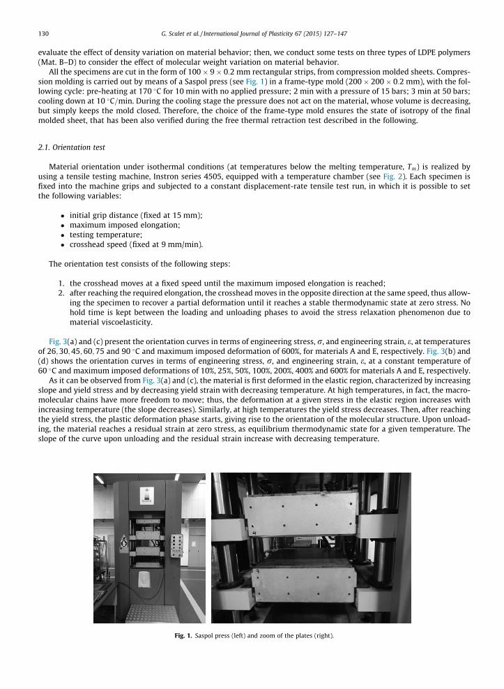
All the specimens are cut in the form of 100� 9� 0:2 mm rectangular strips, from compression molded sheets. Compres-sion molding is carried out by means of a Saspol press (see Fig. 1) in a frame-type mold (200� 200� 0:2 mm), with the fol-lowing cycle: pre-heating at 170 �C for 10 min with no applied pressure; 2 min with a pressure of 15 bars; 3 min at 50 bars;cooling down at 10 �C=min. During the cooling stage the pressure does not act on the material, whose volume is decreasing,but simply keeps the mold closed. Therefore, the choice of the frame-type mold ensures the state of isotropy of the finalmolded sheet, that has been also verified during the free thermal retraction test described in the following.

2.1. Orientation test

Material orientation under isothermal conditions (at temperatures below the melting temperature, Tm) is realized byusing a tensile testing machine, Instron series 4505, equipped with a temperature chamber (see Fig. 2). Each specimen isfixed into the machine grips and subjected to a constant displacement-rate tensile test run, in which it is possible to setthe following variables:

� initial grip distance (fixed at 15 mm);� maximum imposed elongation;� testing temperature;� crosshead speed (fixed at 9 mm/min).

The orientation test consists of the following steps:

1. the crosshead moves at a fixed speed until the maximum imposed elongation is reached;2. after reaching the required elongation, the crosshead moves in the opposite direction at the same speed, thus allow-

ing the specimen to recover a partial deformation until it reaches a stable thermodynamic state at zero stress. Nohold time is kept between the loading and unloading phases to avoid the stress relaxation phenomenon due tomaterial viscoelasticity.

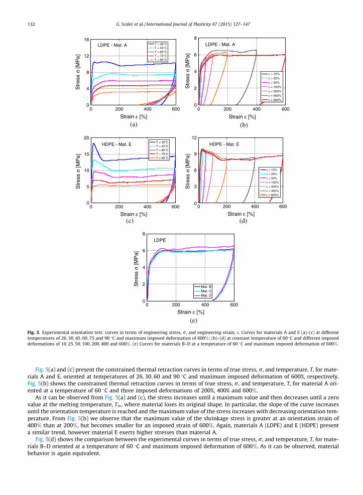
Fig. 3(a) and (c) present the orientation curves in terms of engineering stress, r, and engineering strain, e, at temperaturesof 26;30;45;60;75 and 90 �C and maximum imposed deformation of 600%, for materials A and E, respectively. Fig. 3(b) and(d) shows the orientation curves in terms of engineering stress, r, and engineering strain, e, at a constant temperature of60 �C and maximum imposed deformations of 10%, 25%, 50%, 100%, 200%, 400% and 600% for materials A and E, respectively.

As it can be observed from Fig. 3(a) and (c), the material is first deformed in the elastic region, characterized by increasingslope and yield stress and by decreasing yield strain with decreasing temperature. At high temperatures, in fact, the macro-molecular chains have more freedom to move; thus, the deformation at a given stress in the elastic region increases withincreasing temperature (the slope decreases). Similarly, at high temperatures the yield stress decreases. Then, after reachingthe yield stress, the plastic deformation phase starts, giving rise to the orientation of the molecular structure. Upon unload-ing, the material reaches a residual strain at zero stress, as equilibrium thermodynamic state for a given temperature. Theslope of the curve upon unloading and the residual strain increase with decreasing temperature.

Fig. 1. Saspol press (left) and zoom of the plates (right).

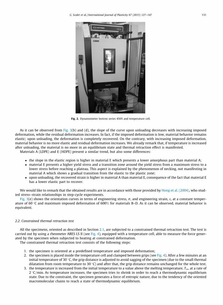
Fig. 2. Dynamometer Instron series 4505 and temperature cell.


As it can be observed from Fig. 3(b) and (d), the slope of the curve upon unloading decreases with increasing imposeddeformation, while the residual deformation increases. In fact, if the imposed deformation is low, material behavior remainselastic; upon unloading, the deformation is completely recovered. On the contrary, with increasing imposed deformation,material behavior is no more elastic and residual deformation increases. We already remark that, if temperature is increasedafter unloading, the material is no more in an equilibrium state and thermal retraction effect is manifested.

Materials A (LDPE) and E (HDPE) present a similar trend, but also some differences:

� the slope in the elastic region is higher in material E which presents a lower amorphous part than material A;� material E presents a higher yield stress and a transition zone around the yield stress from a maximum stress to a

lower stress before reaching a plateau. This aspect is explained by the phenomenon of necking, not manifesting inmaterial A which shows a gradual transition from the elastic to the plastic zone;

� upon unloading, the recovered strain is higher in material A than material E, consequence of the fact that material Ehas a lower elastic part to recover.

We would like to remark that the obtained results are in accordance with those provided by Hong et al. (2004), who stud-ied stress–strain relationships in step-cycle experiments.

Fig. 3(e) shows the orientation curves in terms of engineering stress, r, and engineering strain, e, at a constant temper-ature of 60 �C and maximum imposed deformation of 600% for materials B–D. As it can be observed, material behavior isequivalent.

2.2. Constrained thermal retraction test

All the specimens, oriented as described in Section 2.1, are subjected to a constrained thermal retraction test. The test iscarried out by using a rheometer ARES LS II (see Fig. 4), equipped with a temperature cell, able to measure the force gener-ated by the specimen when subjected to heating at constrained deformation.

The constrained thermal retraction test consists of the following steps:

1. the specimen is oriented at a predefined temperature and imposed deformation;2. the specimen is placed inside the temperature cell and clamped between grips (see Fig. 4). After a few minutes at an

initial temperature of 30 �C, the grip distance is adjusted to avoid sagging of the specimen (due to the small thermaldilatation from room temperature to 30 �C) and after that, the grip distance remains unchanged for the whole test.

3. the temperature is increased from the initial temperature to a value above the melting temperature, Tm, at a rate of2 �C=min. As temperature increases, the specimen tries to shrink in order to reach a thermodynamic equilibriumstate. Due to the constraint, the specimen generates a force of entropic nature, due to the tendency of the orientedmacromolecular chains to reach a state of thermodynamic equilibrium.

0 200 400 6000

4

8

12

16

Strain ε [%]

Str

ess

σ [M

Pa]

T = 26°CT = 45°CT = 60°CT = 75°CT = 90°C

LDPE - Mat. A

(a)

0 200 400 6000

2

4

6

8

Str

ess

σ [M

Pa]

Strain ε [%]

ε = 10%ε = 25%ε = 50%ε = 100%ε = 200%ε = 400%ε = 600%

LDPE - Mat. A

(b)

0 200 400 6000

5

10

15

20

Str

ess

σ [M

Pa]

Strain ε [%]

T = 30°CT = 45°CT = 60°CT = 75°CT = 90°C

HDPE - Mat. E

(c)

0 200 400 6000

3

6

9

12

Str

ess

σ [M

Pa]

Strain ε [%]

ε = 10%ε = 25%ε = 50%ε = 100%ε = 200%ε = 400%ε = 600%

HDPE - Mat. E

(d)

0 200 400 6000

2

4

6

8

Str

ess

σ [M

Pa]

Strain ε [%]

Mat. BMat. CMat. D

LDPE

(e)

Fig. 3. Experimental orientation test: curves in terms of engineering stress, r, and engineering strain, e. Curves for materials A and E (a)–(c) at differenttemperatures of 26;30;45;60;75 and 90 �C and maximum imposed deformation of 600%; (b)–(d) at constant temperature of 60 �C and different imposeddeformations of 10;25;50;100;200;400 and 600%. (e) Curves for materials B–D at a temperature of 60 �C and maximum imposed deformation of 600%.


Fig. 5(a) and (c) present the constrained thermal retraction curves in terms of true stress, r, and temperature, T, for mate-rials A and E, oriented at temperatures of 26;30;60 and 90 �C and maximum imposed deformation of 600%, respectively.Fig. 5(b) shows the constrained thermal retraction curves in terms of true stress, r, and temperature, T, for material A ori-ented at a temperature of 60 �C and three imposed deformations of 200%, 400% and 600%.

As it can be observed from Fig. 5(a) and (c), the stress increases until a maximum value and then decreases until a zerovalue at the melting temperature, Tm, where material loses its original shape. In particular, the slope of the curve increasesuntil the orientation temperature is reached and the maximum value of the stress increases with decreasing orientation tem-perature. From Fig. 5(b) we observe that the maximum value of the shrinkage stress is greater at an orientation strain of400% than at 200%, but becomes smaller for an imposed strain of 600%. Again, materials A (LDPE) and E (HDPE) presenta similar trend, however material E exerts higher stresses than material A.

Fig. 5(d) shows the comparison between the experimental curves in terms of true stress, r, and temperature, T, for mate-rials B–D oriented at a temperature of 60 �C and maximum imposed deformation of 600%. As it can be observed, materialbehavior is again equivalent.

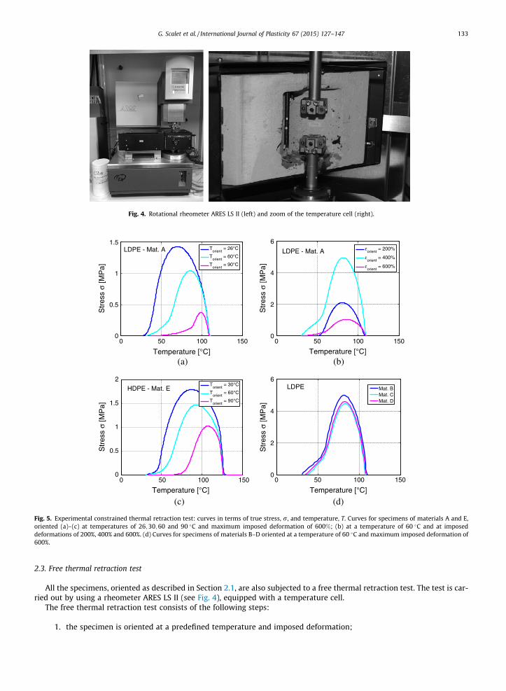
Fig. 4. Rotational rheometer ARES LS II (left) and zoom of the temperature cell (right).

0 50 100 1500

0.5

1

1.5

Str

ess

σ [M

Pa]

Temperature [°C]

Torient

= 26°C

Torient

= 60°C

Torient

= 90°C

LDPE - Mat. A

(a)

0 50 100 1500

2

4

6

Str

ess

σ [M

Pa]

Temperature [°C]

εorient

= 200%

εorient

= 400%

εorient

= 600%

LDPE - Mat. A

(b)

0 50 100 1500

0.5

1

1.5

2

Str

ess

σ [M

Pa]

Temperature [°C]

Torient

= 30°C

Torient

= 60°C

Torient

= 90°C

HDPE - Mat. E

(c)

0 50 100 1500

2

4

6

Str

ess

σ [M

Pa]

Temperature [°C]

Mat. BMat. CMat. D

LDPE

(d)

Fig. 5. Experimental constrained thermal retraction test: curves in terms of true stress, r, and temperature, T. Curves for specimens of materials A and E,oriented (a)–(c) at temperatures of 26;30;60 and 90 �C and maximum imposed deformation of 600%; (b) at a temperature of 60 �C and at imposeddeformations of 200%, 400% and 600%. (d) Curves for specimens of materials B–D oriented at a temperature of 60 �C and maximum imposed deformation of600%.


2.3. Free thermal retraction test

All the specimens, oriented as described in Section 2.1, are also subjected to a free thermal retraction test. The test is car-ried out by using a rheometer ARES LS II (see Fig. 4), equipped with a temperature cell.

The free thermal retraction test consists of the following steps:

1. the specimen is oriented at a predefined temperature and imposed deformation;


2. the specimen is placed inside the temperature cell and clamped between grips (see Fig. 4). After a few minutes at aninitial temperature of 30 �C, the rheometer is put in load-control mode and instructed to keep the load at a verysmall constant tensile level (a few grams). Such a prescribed load is by far too small to cause appreciable deforma-tion of the specimen, but it acts as a set-point, ensuring that the grip distance is automatically and continuouslyadjusted during the test to match the actual specimen length which will decrease on heating due to thermalshrinkage;

3. the test is then conducted by heating up at a rate of 2 �C=min. The oriented specimen, under these test conditions,undergoes a virtually unconstrained thermal shrinkage (the maximum reduction in length at a given temperature ischecked to be equal to that obtained in a free thermal shrinkage test performed by immersing the specimen in anheated silicone oil bath). Our test setup, taking advantage of the load-control mode of the instrument, allows thedirect measurement of the specimen length as a function of temperature during the thermal-shrinkage process.

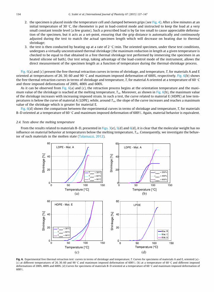
Fig. 6(a) and (c) present the free thermal retraction curves in terms of shrinkage, and temperature, T, for materials A and Eoriented at temperatures of 26;30;60 and 90 �C and maximum imposed deformation of 600%, respectively. Fig. 6(b) showsthe free thermal retraction curves in terms of shrinkage and temperature, T, for material A oriented at a temperature of 60 �Cand three imposed deformations of 200%, 400% and 600%.

As it can be observed from Fig. 6(a) and (c), the retraction process begins at the orientation temperature and the maxi-mum value of the shrinkage is reached at the melting temperature, Tm. Moreover, as shown in Fig. 6(b), the maximum valueof the shrinkage increases with increasing imposed strain. In such a test, the curve related to material E (HDPE) at low tem-peratures is below the curve of material A (LDPE), while, around Tm, the slope of the curve increases and reaches a maximumvalue of the shrinkage which is greater for material E.

Fig. 6(d) shows the comparison between the experimental curves in terms of shrinkage and temperature, T, for materialsB–D oriented at a temperature of 60 �C and maximum imposed deformation of 600%. Again, material behavior is equivalent.

2.4. Tests above the melting temperature

From the results related to materials B–D, presented in Figs. 3(e), 5(d) and 6(d), it is clear that the molecular weight has noinfluence on material behavior at temperatures below the melting temperature, Tm. Consequently, we investigate the behav-ior of such materials in the molten state (Talamazzi, 2012).

0 50 100 1500

20

40

60

Shr

inka

ge [%

]

Temperature [°C]

Torient

= 26°C

Torient

= 60°C

Torient

= 90°C

LDPE - Mat. A

(a)

0 50 100 1500

20

40

60

Shr

inka

ge [%

]

Temperature [°C]

εorient

= 200%

εorient

= 400%

εorient

= 600%

LDPE - Mat. A

(b)

0 50 100 1500

20

40

60

Shr

inka

ge [%

]

Temperature [°C]

Torient

= 30°C

Torient

= 60°C

Torient

= 90°C

HDPE - Mat. E

(c) (d)

LPDE

Fig. 6. Experimental free thermal retraction test: curves in terms of shrinkage and temperature, T. Curves for specimens of materials A and E, oriented (a)–(c) at different temperatures of 26;30;60 and 90 �C and maximum imposed deformation of 600%; (b) at a temperature of 60 �C and different imposeddeformations of 200%, 400% and 600%. (d) Curves for specimens of materials B–D oriented at a temperature of 60 �C and maximum imposed deformation of600%.


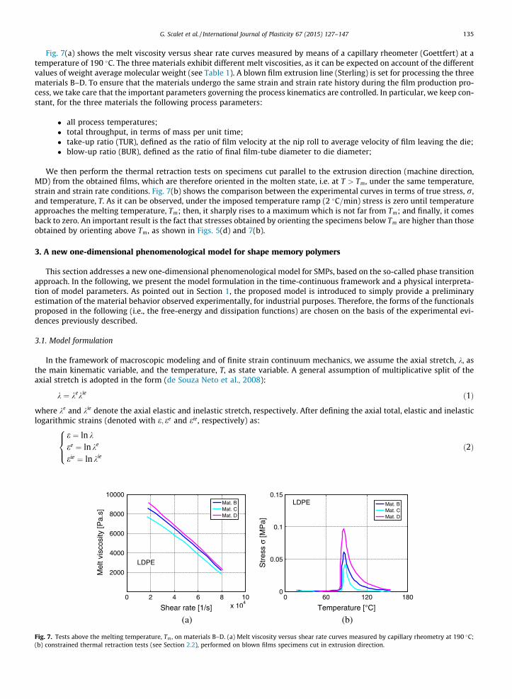
Fig. 7(a) shows the melt viscosity versus shear rate curves measured by means of a capillary rheometer (Goettfert) at atemperature of 190 �C. The three materials exhibit different melt viscosities, as it can be expected on account of the differentvalues of weight average molecular weight (see Table 1). A blown film extrusion line (Sterling) is set for processing the threematerials B–D. To ensure that the materials undergo the same strain and strain rate history during the film production pro-cess, we take care that the important parameters governing the process kinematics are controlled. In particular, we keep con-stant, for the three materials the following process parameters:

� all process temperatures;� total throughput, in terms of mass per unit time;� take-up ratio (TUR), defined as the ratio of film velocity at the nip roll to average velocity of film leaving the die;� blow-up ratio (BUR), defined as the ratio of final film-tube diameter to die diameter;

We then perform the thermal retraction tests on specimens cut parallel to the extrusion direction (machine direction,MD) from the obtained films, which are therefore oriented in the molten state, i.e. at T > Tm, under the same temperature,strain and strain rate conditions. Fig. 7(b) shows the comparison between the experimental curves in terms of true stress, r,and temperature, T. As it can be observed, under the imposed temperature ramp (2 �C=min) stress is zero until temperatureapproaches the melting temperature, Tm; then, it sharply rises to a maximum which is not far from Tm; and finally, it comesback to zero. An important result is the fact that stresses obtained by orienting the specimens below Tm are higher than thoseobtained by orienting above Tm, as shown in Figs. 5(d) and 7(b).

3. A new one-dimensional phenomenological model for shape memory polymers

This section addresses a new one-dimensional phenomenological model for SMPs, based on the so-called phase transitionapproach. In the following, we present the model formulation in the time-continuous framework and a physical interpreta-tion of model parameters. As pointed out in Section 1, the proposed model is introduced to simply provide a preliminaryestimation of the material behavior observed experimentally, for industrial purposes. Therefore, the forms of the functionalsproposed in the following (i.e., the free-energy and dissipation functions) are chosen on the basis of the experimental evi-dences previously described.

3.1. Model formulation

In the framework of macroscopic modeling and of finite strain continuum mechanics, we assume the axial stretch, k, asthe main kinematic variable, and the temperature, T, as state variable. A general assumption of multiplicative split of theaxial stretch is adopted in the form (de Souza Neto et al., 2008):

Fig. 7.(b) con

k ¼ kekie ð1Þ

where ke and kie denote the axial elastic and inelastic stretch, respectively. After defining the axial total, elastic and inelasticlogarithmic strains (denoted with e; ee and eie, respectively) as:

e ¼ ln k

ee ¼ ln ke

eie ¼ ln kie

8><>: ð2Þ

0 2 4 6 8 10x 10

4

2000

4000

6000

8000

10000

Mel

t vis

cosi

ty [P

a.s]

Shear rate [1/s]

Mat. BMat. CMat. D

LDPE

(a)

0 60 120 1800

0.05

0.1

0.15

Str

ess

σ [M

Pa]

Temperature [°C]

Mat. BMat. CMat. D

LDPE

(b)

Tests above the melting temperature, Tm , on materials B–D. (a) Melt viscosity versus shear rate curves measured by capillary rheometry at 190 �C;strained thermal retraction tests (see Section 2.2), performed on blown films specimens cut in extrusion direction.


we rewrite Eq. (1), as follows:

e ¼ ee þ eie ð3Þ

Recalling the discussion of Section 1, the phenomenon of thermal retraction in PE-based polymers is a shape memoryproperty and it is strongly connected with molecules orientation under mechanical and thermal loads. Thus, in the phasetransition framework, the main idea is that the microscopic structure of the polymer can be represented by a suitable scalarparameter, the so-called phase parameter, able to describe which kind of microstructure is present. In order to introduce asuitable phase parameter, we start by viewing the semi-crystalline polymer as composed of chains of type A, which are in thecrystalline phase, and chains of type B, which are in the amorphous phase and can be (non)oriented by mechanical or ther-mal loads. Then, as shape memory in semi-crystalline polymers strongly depends on the orientation of the polymer chains,we assume the state variable, v, as a phase parameter describing the non-oriented microstructure and related to the localproportion of non-oriented chains of type B with respect to the oriented phase. Due to its physical meaning, the phaseparameter has to be between 0 and 1, i.e., v 2 ½0;1�. In particular, the case v ¼ 1 corresponds to the presence of completelynon-oriented chains, while the case v ¼ 0 stands for complete ordered chains.

We choose the inelastic logarithmic strain, eie ¼ eie T;vð Þ, as follows:

eie ¼ Ca expa

T � T0

� �1� vð Þ ð4Þ

with Ca and a positive material parameters and T0 a reference temperature.

3.1.1. Helmholtz free-energy functionThe Helmholtz free-energy function, W ¼ W e; T;vð Þ, is assumed in the following classical form:

W ¼ 12

E eeð Þ2 � csT ln T þ I 0;1½ � vð Þ ð5Þ

that, after introducing Eq. (3), becomes:

W ¼ 12

E e� eie� �2 � csT ln T þ I 0;1½ � vð Þ ð6Þ

where cs > 0 is the specific heat (assumed constant for the sake of simplicity) and I 0;1½ � vð Þ is the indicator function forcing tofulfill the constraints on v, defined as (Nguyen and Moumni, 1995a,b):

I½0;1�ðvÞ ¼0 if 0 6 v � 1þ1 otherwise

�ð7Þ

The function E ¼ E T;vð Þ represents the Young’s modulus, that, according to experimental evidences of Fig. 3(a)–(d), weassume to strongly depend on temperature, T, and on phase, v, as follows:

E ¼ expb

T � T0

� �1

vE1þ 1�v

E0

ð8Þ

E1 and E0 being positive parameters due to material rigidity for the two cases v ¼ 1 and v ¼ 0, respectively (with E1 > E0),and b a positive material parameter. In particular, we assume that at constant temperature, T, the Young’s modulus dependson the phase, v, following the classical model of Reuss, while at constant phase, v, the Young’s modulus depends exponen-tially on temperature, T, as manifested in Fig. 3(a)–(d). The reader is referred to Appendix A for a discussion on the adoptedexpression for the Young’s modulus.

3.1.2. Constitutive equationsStarting from the free-energy, W, presented in Eq. (6), and following standard arguments (de Souza Neto et al., 2008), we

derive the Kirchhoff axial stress, s:

s ¼ @W@ee ¼ E e� eie

� �¼ exp

bT � T0

� �1

vE1þ 1�v

E0

e� Ca expa

T � T0

� �1� vð Þ

� �ð9Þ

as well as the thermodynamic force, Xnd, governing the evolution of v:

Xnd ¼ � @W@v ¼ �

12@E@v e� eie� �2 þ E e� eie

� � @eie

@v � c ¼ �12@E@v

s2

E2 þ@eie

@v s� c

¼ � 12

expb

T � T0

� �E1 � E0ð ÞE1E0

E0vþ E1 1� vð Þð Þ2e� Ca exp

aT � T0

� �1� vð Þ

� �2

� Ca expaþ bT � T0

� �1

vE1þ 1�v

E0

e� Ca expa

T � T0

� �1� vð Þ

� �� c ð10Þ


Here, c 2 @I 0;1½ � vð Þ, with @I 0;1½ � vð Þ the subdifferential of the indicator function I 0;1½ � vð Þ, taken in the sense of convex analysis(Brézis, 1973):

@I 0;1½ � vð Þ ¼c0 � 0 if v ¼ 00 if 0 < v < 1c1 P 0 if v ¼ 1

8><>: ð11Þ

We can associate to Eq. (11) the classical Kuhn–Tucker complementarity conditions, as follows:

v P 0; c06 0; c0v ¼ 0

v� 1ð Þ 6 0; c1 P 0; c1 v� 1ð Þ ¼ 0

(ð12Þ

3.1.3. Evolution equations and limit functions

We define a limit function, F ¼ F Xnd; T

, playing the role of yield function (Lubliner, 1990), in the following form:

F ¼ Xnd þ g2

�� g2

ð13Þ

where g ¼ g T;vð Þ is a sufficiently smooth function, governing the yield level of stress activating the phase transition, i.e., theorientation process:

g ¼ Cg expEg

T � T0

� �þ h1 exp

Eh1

T � T0

� �ð1� vÞ þ h2 exp

Eh2

T � T0

� �ð1� vÞ2 þ h3 exp

Eh3

T � T0

� �ð1� vÞ3 ð14Þ

Cg and Eg being positive material parameters and h1;h2;h3; Eh1 ; Eh2 , and Eh3 positive material constants describing materialhardening.

Then, as traditionally done in the context of associative evolution, we assume the evolution equation of v, as follows:

_v ¼ _fXnd þ g

2

Xnd þ g2

�� ð15Þ

where _f is a non-negative consistency parameter.The model is finally completed by the classical Kuhn–Tucker conditions, as follows:

_f P 0; F 6 0; _fF ¼ 0 ð16Þ

3.1.4. Dissipation functionAlthough the proposed model relies on an yield surface-based formulation, we complete the description by recalling that

the yield surface condition (13) can be equivalently converted in a pseudo-potential of dissipation, / ¼ / _v; Tð Þ, which is apositive convex functional depending on dissipative variables, vanishing for vanishing dissipation, in particular in the form:

/ ¼�g _v if _v � 00 if _v > 0

�ð17Þ

We remark that, once defined the pseudo-potential of dissipation, /, we can prescribe the constitutive relation for theinternal force, X, responsible for the phase transition, as follows (Frémond, 2002; Frémond, 2012; Gurtin et al., 2010;Halphen and Nguyen, 1975, 1974):

X ¼ �Xnd þ Xd ¼ @W@v þ

@/@ _v ð18Þ

In particular, two contributions are considered, i.e., a non-dissipative term, Xnd, and a dissipative term, Xd. The constitu-tive relation for the internal non-dissipative force, Xnd, is given in Eq. (10), while the constitutive relation for the dissipativeforce, Xd, is:

Xd ¼ @/@ _v ¼

�g if _v � 00 if _v > 0

�ð19Þ

From the definition of X, presented in Eq. (18), we can then derive the limit function introduced in Eq. (13). We note thatsuch an approach, similar to that employed in shape memory alloy modeling, considers a translation of the thermodynamicforce, Xnd, to allow the phase transformation in the thermal retraction case for which Xnd ¼ 0, i.e., s ¼ 0.

Therefore, the evolution of the phase, v, depends on the internal force, X, which is included in the energy balance of thesystem. We obtain the following balance equation:

X ¼ �Xnd þ Xd ¼ 0 ð20Þ


after assuming that no micro-forces are applied to activate the orientation of polymer chains. From Eq. (20) we can derive theevolution equation of the phase parameter, v, as follows:

Fig. 8.assumi

_v ¼ @I �g;0½ � Xnd

ð21Þ

that can then rewritten as Eq. (15).

3.1.5. Physical interpretation of model parametersIdeally, the identification procedure of a material model should be automated using optimization techniques. In the fol-

lowing sections, all model parameters are calibrated through a trial and error procedure to best fit the experimental orien-tation curves of Fig. 3(a) and (c), related to materials A and E.

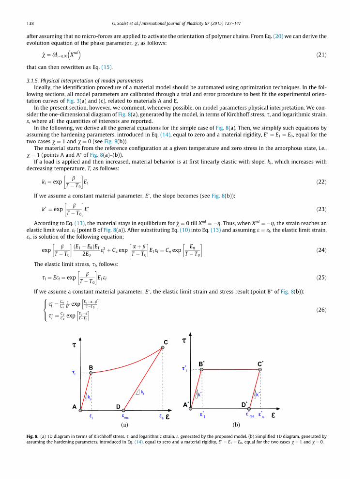
In the present section, however, we comment, whenever possible, on model parameters physical interpretation. We con-sider the one-dimensional diagram of Fig. 8(a), generated by the model, in terms of Kirchhoff stress, s, and logarithmic strain,e, where all the quantities of interests are reported.

In the following, we derive all the general equations for the simple case of Fig. 8(a). Then, we simplify such equations byassuming the hardening parameters, introduced in Eq. (14), equal to zero and a material rigidity, E� ¼ E1 ¼ E0, equal for thetwo cases v ¼ 1 and v ¼ 0 (see Fig. 8(b)).

The material starts from the reference configuration at a given temperature and zero stress in the amorphous state, i.e.,v ¼ 1 (points A and A⁄ of Fig. 8(a)–(b)).

If a load is applied and then increased, material behavior is at first linearly elastic with slope, ki, which increases withdecreasing temperature, T, as follows:

ki ¼ expb

T � T0

� �E1 ð22Þ

If we assume a constant material parameter, E�, the slope becomes (see Fig. 8(b)):

k� ¼ expb

T � T0

� �E� ð23Þ

According to Eq. (13), the material stays in equilibrium for _v ¼ 0 till Xnd ¼ �g. Thus, when Xnd ¼ �g, the strain reaches anelastic limit value, el (point B of Fig. 8(a)). After substituting Eq. (10) into Eq. (13) and assuming e ¼ el, the elastic limit strain,el, is solution of the following equation:

expb

T � T0

� �E1 � E0ð ÞE1

2E0e2

l þ Ca expaþ bT � T0

� �E1el ¼ Cg exp

Eg

T � T0

� �ð24Þ

The elastic limit stress, sl, follows:

sl ¼ Eel ¼ expb

T � T0

� �E1el ð25Þ

If we assume a constant material parameter, E�, the elastic limit strain and stress result (point B⁄ of Fig. 8(b)):

e�l ¼CgCa

1E� exp Eg�a�b

T�T0

h is�l ¼

CgCa

exp Eg�aT�T0

h i8><>: ð26Þ

(a) (b)

(a) 1D diagram in terms of Kirchhoff stress, s, and logarithmic strain, e, generated by the proposed model. (b) Simplified 1D diagram, generated byng the hardening parameters, introduced in Eq. (14), equal to zero and a material rigidity, E� ¼ E1 ¼ E0, equal for the two cases v ¼ 1 and v ¼ 0.


Since experimental evidences of Fig. 3(a)–(d) shows that the elastic limit strain decreases with decreasing temperatureand the elastic limit stress increases with decreasing temperature, we derive the following constraints on model parametersfrom system of Eqs. (26):

Eg < aþ b

Eg > a

�ð27Þ

If the load further increases, inelastic deformations start to develop and the orientation process starts. As it can beobserved, the hardening parameters are responsible for the stress–strain curve between points B and C of Fig. 8(a). Thechoice of g reported in Eq. (14) is due to experimental observations. Once the imposed level of load is reached, the orienta-tion process reaches a certain level of orientation (point C of Fig. 8(a)), where v ¼ bv and e ¼ es. In the particular case of com-pleted orientation process, i.e., v ¼ bv ¼ 0, the maximum transformation strain, emax, is reached. If we assume a constantmaterial parameter, E�, and no hardening (i.e., inelastic deformations start to develop at constant elastic limit stress, sl),the maximum transformation strain becomes:

e�max ¼Cg

Ca

1E�

expEg � a� b

T � T0

� �þ Ca exp

aT � T0

� �ð28Þ

and increases with decreasing temperature, T, thus reproducing experimental evidences of Fig. 3(a)–(d).If we start to unload from point C of Fig. 8(a), we evolve in the region for which _v ¼ 0. The slope upon unloading, kf ,

follows:

kf ¼ expb

T � T0

� �1bv

E1þ 1�bv

E0

ð29Þ

and increases with decreasing temperature, T, and with increasing v, as experimentally observed in Fig. 3(a)–(d). If weassume a constant material parameter, E�, the slope upon unloading becomes (point C⁄ of Fig. 8(b)):

k� ¼ expb

T � T0

� �E� ð30Þ

Upon unloading, when s ¼ 0 and thus Xnd ¼ 0, a residual strain, eres ¼ e�res, is present (points D and D⁄ of Fig. 8(a)–(b)), inthe following form:

eres ¼ Ca expa

T � T0

� �1� bv� �

ð31Þ

which increases with decreasing temperature, T, and phase, v.If we start increasing temperature from point D of Fig. 8(a) at s ¼ 0 and no constraints on the material (free thermal

retraction), the residual strain, eres, can be partially recovered.On the other hand, if we start increasing temperature at fixed e ¼ eres from point D of Fig. 8(a) (constrained thermal

retraction), we obtain, after assuming a constant material parameter, E�:

s ¼ E� exp bT�T0

h ieres � Ca exp a

T�T0

h i1� bv� �

Xnd ¼ �Ca exp aT�T0

h is

8><>: ð32Þ

Moreover, we observe that at point D, we have _v > 0 and this last remark justifies irreversibility of the retraction processat s ¼ 0.

4. Time-discrete framework

We now elaborate on a possible algorithmic treatment of model equations. For the sake of notation simplicity, we usesuperscript n for all the variables evaluated at time tn, while we drop superscript nþ 1 for all the variables computed at timetnþ1.

We start making use of a classical backward-Euler integration algorithm for the evolution Eq. (15). In this sense, the time-discretized evolution equation is given by:

v� vn � DfXnd þ g

2

Xnd þ g2

�� ¼ 0 ð33Þ

where Df ¼R tnþ1

tn_fdt is the time-integrated consistency parameter.

In the model, since we deal with one phase parameter involving constraints, we adopt the approach consisting in thereplacement of the Kuhn–Tucker complementarity inequality conditions, a 6 0; b P 0; ab ¼ 0; a; b 2 R, by the equivalentFischer–Burmeister complementarity function U (Fischer, 1992), with U : R2 ! R and defined as follows:


Uða; bÞ ¼ffiffiffiffiffiffiffiffiffiffiffiffiffiffiffiffia2 þ b2

pþ a� b, such that Uða; bÞ ¼ 0() a 6 0; b P 0; ab ¼ 0. Such a definition allows to rewrite the comple-

mentarity inequality constraints as a non-linear equality constraint through the application of the Fischer–Burmeister com-plementarity function. Therefore, we substitute the discrete Kuhn–Tucker conditions deriving from Eq. (16) by the followingfunction in the time-discrete frame:
ffiffiffiffiffiffiffiffiffiffiffiffiffiffiffiffiffiffiffi
F2 þ Df2q

þ F � Df ¼ 0 ð34Þ

The same strategy can be employed to treat the set of inequalities given by the constraint on v. In fact, the additionalKuhn–Tucker conditions (12) can be substituted by the equivalent equalities:
ffiffiffiffiffiffiffiffiffiffiffiffiffiffiffiffiffiffiffiffiffiffi
v2 þ ðc0Þ2q

þ c0 � v ¼ 0ffiffiffiffiffiffiffiffiffiffiffiffiffiffiffiffiffiffiffiffiffiffiffiffiffiffiffiffiffiffiffiffiffiffiv� 1ð Þ2 þ ðc1Þ2

qþ v� 1ð Þ � c1 ¼ 0

8><>: ð35Þ

The time-discrete problem, Q ¼ Q e;hð Þ, evaluated at time tnþ1, takes the specific form:

Q ¼

v� vn � DfXndþg

2

Xndþg2j jffiffiffiffiffiffiffiffiffiffiffiffiffiffiffiffiffiffiffi

F2 þ Df2q

þ F � Dfffiffiffiffiffiffiffiffiffiffiffiffiffiffiffiffiffiffiffiffiffiffiv2 þ ðc0Þ2

qþ c0 � vffiffiffiffiffiffiffiffiffiffiffiffiffiffiffiffiffiffiffiffiffiffiffiffiffiffiffiffiffiffiffiffiffiffi

v� 1ð Þ2 þ ðc1Þ2q

þ v� 1ð Þ � c1

26666666664

37777777775ð36Þ

with h ¼ v;Df; c0; c1 �

. The active set can now be determined via the solution of the following non-linear system ofequations:

Q ¼ 0 ð37Þ

by using a classical Newton–Raphson method.All the model equations and numerical examples presented in Section 5 are implemented in two Mathematica (Wolfram,

2013) packages, AceGen and AceFEM (Korelc, 2009). These systems allow to automatically obtain explicit expressions result-ing from differentiation. In particular, the tangent matrix is computed analytically and factorized at each iteration. This leadto a quadratic convergence rate of the Newton method (Quarteroni et al., 2007). In Appendix B we provide the tangentmatrix deriving from the time-discrete problem (36).

We remark that, since the Fischer–Burmeister complementary function, U, is non-differentiable at 0;0ð Þ, we make use of a

regularized counterpart, Ud, defined as Udða; b; dÞ ¼ffiffiffiffiffiffiffiffiffiffiffiffiffiffiffiffiffiffiffiffiffiffiffiffiffiffiffiffiffia2 þ b2 þ 2d2

pþ a� b, such that Udða; b; dÞ ¼ 0() a 6 0; b P 0;

ab ¼ �d2, where d is a positive regularization parameter (Kanzow, 1996).

5. Numerical results

In this Section we test the validity of the proposed model as well as its algorithm through some numerical simulationsand comparisons with experimental results described in Section 2. The purpose is to emphasize model prediction capabilitiesthrough a qualitative and then quantitative validation with experimental data.

All the results presented in the following are expressed in terms of engineering stresses and strains. The derivation ofengineering stresses from the Kirchhoff stress, s, defined in Eq. (9), is possible under the hypothesis of material incompress-ibility, which is valid for the material under investigation (Hiss et al., 1999).

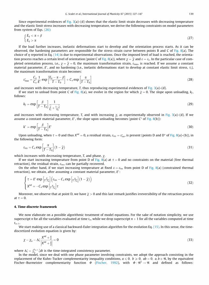
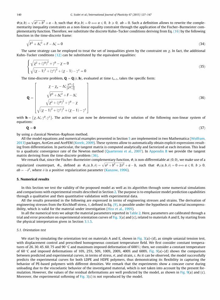
In all the numerical tests we adopt the material parameters reported in Table 2. Here, parameters are calibrated through atrial and error procedure on experimental orientation curves of Fig. 3(a) and (c), related to materials A and E, by starting fromthe physical interpretation given in Section 3.1.5.

5.1. Orientation test

We start by simulating the orientation test on materials A and E, shown in Fig. 3(a)–(d), as simple uniaxial tension test,with displacement control and prescribed homogeneous constant temperature field. We first consider constant tempera-tures of 26;30;45;60;75 and 90 �C and maximum imposed deformation of 600%; then, we consider a constant temperatureof 60 �C and imposed deformations of 10%, 25%, 50%, 100%, 200%, 400% and 600%. Fig. 9(a)–(d) shows the comparisonbetween predicted and experimental curves, in terms of stress, r, and strain, e. As it can be observed, the model successfullypredicts the experimental curves for both LDPE and HDPE polymers, thus demonstrating its flexibility in capturing thebehavior of PE-based polymers with different densities. We remark that the experiments show a concave curve duringunloading due to the viscoelastic behavior of the investigated material, which is not taken into account by the present for-mulation. However, the values of the residual deformations are well predicted by the model, as shown in Fig. 9(a) and (c).Moreover, the experimental softening of Fig. 3(c) is not reproduced by the model.

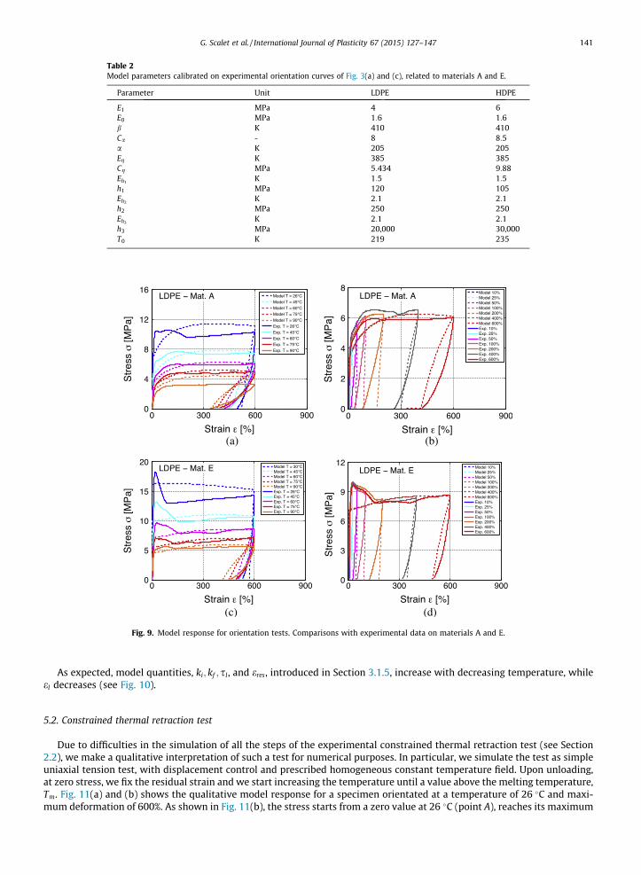
Table 2Model parameters calibrated on experimental orientation curves of Fig. 3(a) and (c), related to materials A and E.

Parameter Unit LDPE HDPE

E1 MPa 4 6E0 MPa 1:6 1:6b K 410 410Ca - 8 8:5a K 205 205Eg K 385 385Cg MPa 5:434 9:88Eh1

K 1:5 1:5h1 MPa 120 105Eh2

K 2:1 2:1h2 MPa 250 250Eh3

K 2:1 2:1h3 MPa 20,000 30,000T0 K 219 235

Fig. 9. Model response for orientation tests. Comparisons with experimental data on materials A and E.


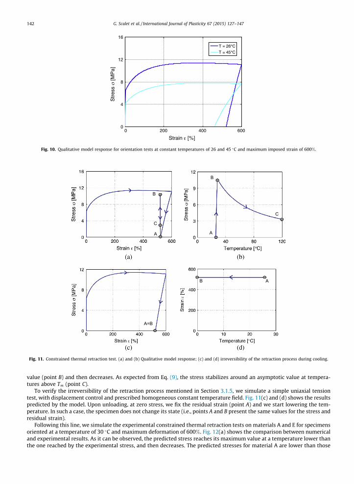
As expected, model quantities, ki; kf ; sl, and eres, introduced in Section 3.1.5, increase with decreasing temperature, whileel decreases (see Fig. 10).

5.2. Constrained thermal retraction test

Due to difficulties in the simulation of all the steps of the experimental constrained thermal retraction test (see Section2.2), we make a qualitative interpretation of such a test for numerical purposes. In particular, we simulate the test as simpleuniaxial tension test, with displacement control and prescribed homogeneous constant temperature field. Upon unloading,at zero stress, we fix the residual strain and we start increasing the temperature until a value above the melting temperature,Tm. Fig. 11(a) and (b) shows the qualitative model response for a specimen orientated at a temperature of 26 �C and maxi-mum deformation of 600%. As shown in Fig. 11(b), the stress starts from a zero value at 26 �C (point A), reaches its maximum

0 200 400 6000

4

8

12

16

Str

ess

[MP

a]

Strain [%]

Fig. 10. Qualitative model response for orientation tests at constant temperatures of 26 and 45 �C and maximum imposed strain of 600%.

B

C

A

A=B

B A

A

C

B

Fig. 11. Constrained thermal retraction test. (a) and (b) Qualitative model response; (c) and (d) irreversibility of the retraction process during cooling.


value (point B) and then decreases. As expected from Eq. (9), the stress stabilizes around an asymptotic value at tempera-tures above Tm (point C).

To verify the irreversibility of the retraction process mentioned in Section 3.1.5, we simulate a simple uniaxial tensiontest, with displacement control and prescribed homogeneous constant temperature field. Fig. 11(c) and (d) shows the resultspredicted by the model. Upon unloading, at zero stress, we fix the residual strain (point A) and we start lowering the tem-perature. In such a case, the specimen does not change its state (i.e., points A and B present the same values for the stress andresidual strain).

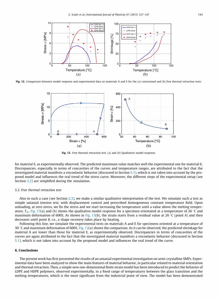
Following this line, we simulate the experimental constrained thermal retraction tests on materials A and E for specimensoriented at a temperature of 30 �C and maximum deformation of 600%. Fig. 12(a) shows the comparison between numericaland experimental results. As it can be observed, the predicted stress reaches its maximum value at a temperature lower thanthe one reached by the experimental stress, and then decreases. The predicted stresses for material A are lower than those

0 50 100 1500

3

6

9

12

Str

ess

[MP

a]

LDPE Mat. ALDPE ModelHDPE Mat. EHDPE Model

(a)

0 50 100 1500

25

50

75

100

Shr

inka

ge [%

]

LDPE Mat. A

LDPE Model

HDPE Mat. E

HDPE Model

(b)

Fig. 12. Comparison between model response and experimental data on materials A and E for the (a) constrained and (b) free thermal retraction tests.

B A

A

B

Fig. 13. Free thermal retraction test. (a) and (b) Qualitative model response.


for material E, as experimentally observed. The predicted maximum value matches well the experimental one for material E.Discrepancies, especially in terms of concavities of the curves and temperature ranges, are attributed to the fact that theinvestigated material manifests a viscoelastic behavior (discussed in Section 5.1), which is not taken into account by the pro-posed model and influences the real trend of the stress curve. Moreover, the different steps of the experimental setup (seeSection 2.2) are simplified during the simulation.

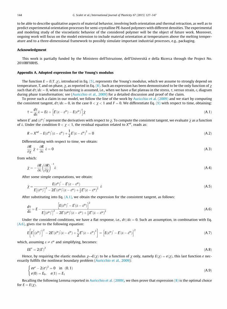
5.3. Free thermal retraction test

Also in such a case (see Section 2.3), we make a similar qualitative interpretation of the test. We simulate such a test assimple uniaxial tension test, with displacement control and prescribed homogeneous constant temperature field. Uponunloading, at zero stress, we fix the stress and we start increasing the temperature until a value above the melting temper-ature, Tm. Fig. 13(a) and (b) shows the qualitative model response for a specimen orientated at a temperature of 26 �C andmaximum deformation of 600%. As shown in Fig. 13(b), the strain starts from a residual value at 26 �C (point A) and thendecreases until point B, i.e., a shape recovery takes place by heating.

Following this line, we simulate the experimental tests on materials A and E for specimens oriented at a temperature of30 �C and maximum deformation of 600%. Fig. 12(a) shows the comparison. As it can be observed, the predicted shrinkage formaterial A are lower than those for material E, as experimentally observed. Discrepancies in terms of concavities of thecurves are again attributed to the fact that the investigated material manifests a viscoelastic behavior (discussed in Section5.1), which is not taken into account by the proposed model and influences the real trend of the curve.

6. Conclusions

The present work has first presented the results of an uniaxial experimental investigation on semi-crystalline SMPs. Exper-imental data have been analyzed to show the main features of material behavior, in particular related to material orientationand thermal retraction. Then, a simple new one-dimensional finite strain model has been introduced to predict the behavior ofLDPE and HDPE polymers, observed experimentally, in a fixed range of temperatures between the glass transition and themelting temperatures, which is the most significant from the industrial point of view. The model has been demonstrated


to be able to describe qualitative aspects of material behavior, involving both orientation and thermal retraction, as well as topredict experimental orientation processes for semi-crystalline PE-based polymers with different densities. The experimentaland modeling study of the viscoelastic behavior of the considered polymer will be the object of future work. Moreover,ongoing work will focus on the model extension to include material orientation at temperatures above the melting temper-ature and to a three-dimensional framework to possibly simulate important industrial processes, e.g., packaging.

Acknowledgment

This work is partially funded by the Ministero dell’Istruzione, dell’Università e della Ricerca through the Project No.2010BFXRHS.

Appendix A. Adopted expression for the Young’s modulus

The function E ¼ E T;vð Þ, introduced in Eq. (5), represents the Young’s modulus, which we assume to strongly depend ontemperature, T, and on phase, v, as reported in Eq. (8). Such an expression has been demonstrated to be the only function of vsuch that ds=de ¼ 0, when no hardening is assumed, i.e., when we have a flat plateau in the stress, s, versus strain, e, diagramduring phase transformation; see (Auricchio et al., 2009) for a detailed discussion and proof of the claim.

To prove such a claim in our model, we follow the line of the work by Auricchio et al. (2009) and we start by computingthe consistent tangent, ds=de ¼ 0, in the case 0 < v < 1 and F ¼ 0. We differentiate Eq. (9) with respect to time, obtaining:

_s ¼ dsde

_e ¼ E _eþ E0ðe� eieÞ � EðeieÞ0h i

_v ðA:1Þ

where E0 and ðeieÞ0 represent the derivatives with respect to v. To compute the consistent tangent, we evaluate _v as a functionof _e. Under the condition 0 < v < 1, the residual equation related to Xnd, reads as:

R ¼ Xnd � EðeieÞ0ðe� eieÞ þ 12

E0ðe� eieÞ2 ¼ 0 ðA:2Þ

Differentiating with respect to time, we obtain:

@R@v

_vþ @R@e

_e ¼ 0 ðA:3Þ

from which:

_v ¼ � @R@e

@R@v

� ��1

_e ðA:4Þ

After some simple computations, we obtain:

_v ¼ EðeieÞ0 � E0ðe� eieÞE ðeieÞ0� �2 � 2E0ðeieÞ0ðe� eieÞ þ 1

2 E00 e� eieð Þ2_e ðA:5Þ

After substituting into Eq. (A.1), we obtain the expression for the consistent tangent, as follows:

dsde¼ E�

EðeieÞ0 � E0ðe� eieÞh i2

E ðeieÞ0� �2 � 2E0ðeieÞ0ðe� eieÞ þ 1

2 E00 e� eieð Þ2ðA:6Þ

Under the considered conditions, we have a flat response, i.e., ds=de ¼ 0. Such an assumption, in combination with Eq.(A.6), gives rise to the following equation:

E E ðeieÞ0h i2

� 2E0ðeieÞ0ðe� eieÞ þ 12

E00ðe� eieÞ2� �

¼ EðeieÞ0 � E0ðe� eieÞh i2

ðA:7Þ

which, assuming e – eie and simplifying, becomes:

EE00 ¼ 2ðE0Þ2 ðA:8Þ

Hence, by requiring the elastic modulus v#EðvÞ to be a function of v only, namely EðvÞ ¼ eðvÞ, this last function e nec-essarily fulfills the nonlinear boundary problem (Auricchio et al., 2009):

ee00 � 2ðe0Þ2 ¼ 0 in ð0;1Þeð0Þ ¼ E0; eð1Þ ¼ E1

(ðA:9Þ

Recalling the following Lemma reported in Auricchio et al. (2009), we then prove that expression (8) is the optimal choicefor E ¼ EðvÞ.


Lemma. The function t#1= v=E1 þ 1� vð Þ=E0½ � is the only classical solution of the nonlinear boundary value problem (A.9).The reader is referred to the work by Auricchio et al. (2009) for the proof of the above Lemma.

Appendix B. Newton–Raphson method

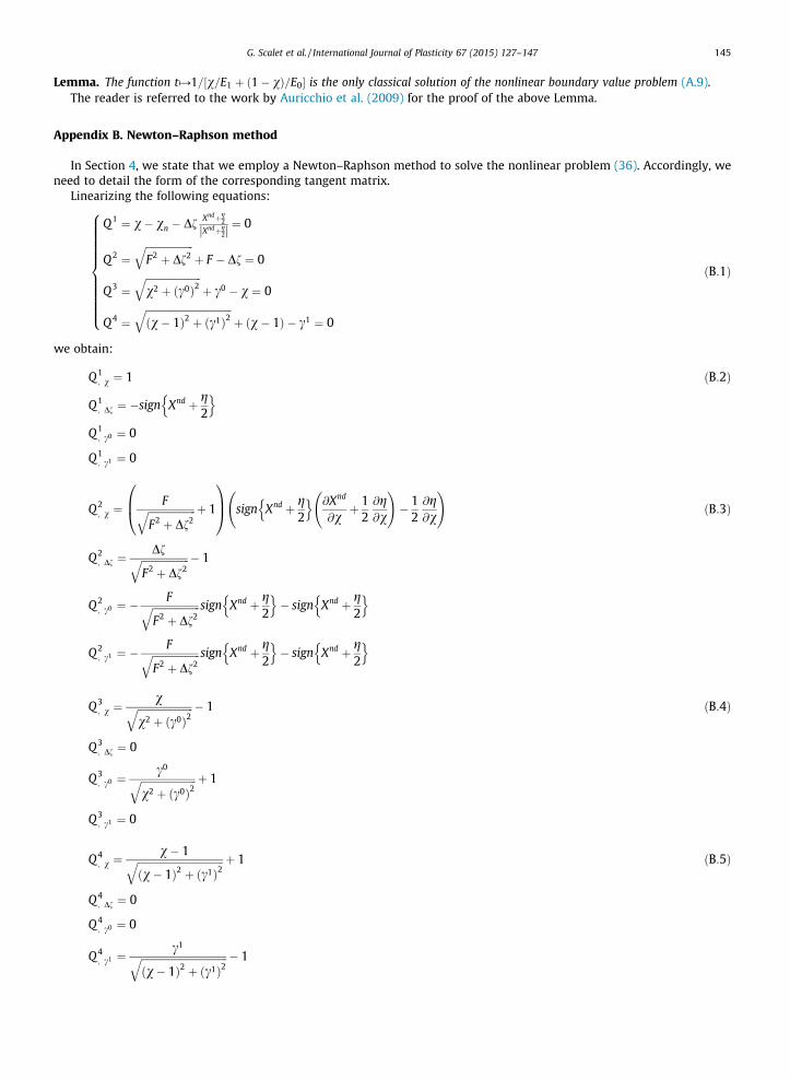
In Section 4, we state that we employ a Newton–Raphson method to solve the nonlinear problem (36). Accordingly, weneed to detail the form of the corresponding tangent matrix.

Linearizing the following equations:

Q 1 ¼ v� vn � DfXndþg

2

Xndþg2j j ¼ 0

Q 2 ¼ffiffiffiffiffiffiffiffiffiffiffiffiffiffiffiffiffiffiffiF2 þ Df2

qþ F � Df ¼ 0

Q 3 ¼ffiffiffiffiffiffiffiffiffiffiffiffiffiffiffiffiffiffiffiffiffiffiv2 þ ðc0Þ2

qþ c0 � v ¼ 0

Q 4 ¼ffiffiffiffiffiffiffiffiffiffiffiffiffiffiffiffiffiffiffiffiffiffiffiffiffiffiffiffiffiffiffiffiffiffiv� 1ð Þ2 þ ðc1Þ2

qþ v� 1ð Þ � c1 ¼ 0

8>>>>>>>>>><>>>>>>>>>>:ðB:1Þ

we obtain:

Q 1; v ¼ 1 ðB:2Þ

Q 1; Df ¼ �sign Xnd þ g

2

n oQ 1; c0 ¼ 0

Q 1; c1 ¼ 0

Q 2; v ¼

FffiffiffiffiffiffiffiffiffiffiffiffiffiffiffiffiffiffiffiF2 þ Df2

q þ 1

0B@1CA sign Xnd þ g

2

n o @Xnd

@v þ12@g@v

!� 1

2@g@v

!ðB:3Þ

Q 2; Df ¼

DfffiffiffiffiffiffiffiffiffiffiffiffiffiffiffiffiffiffiffiF2 þ Df2

q � 1

Q 2; c0 ¼ �


q sign Xnd þ g2

n o� sign Xnd þ g

2

n o

Q 2; c1 ¼ �


q sign Xnd þ g2

n o� sign Xnd þ g

2

n o

Q 3; v ¼

vffiffiffiffiffiffiffiffiffiffiffiffiffiffiffiffiffiffiffiffiffiffiv2 þ ðc0Þ2

q � 1 ðB:4Þ

Q 3; Df ¼ 0

Q 3; c0 ¼

c0ffiffiffiffiffiffiffiffiffiffiffiffiffiffiffiffiffiffiffiffiffiffiv2 þ ðc0Þ2

q þ 1

Q 3; c1 ¼ 0

Q 4; v ¼

v� 1ffiffiffiffiffiffiffiffiffiffiffiffiffiffiffiffiffiffiffiffiffiffiffiffiffiffiffiffiffiffiffiffiffiffiðv� 1Þ2 þ ðc1Þ2

q þ 1 ðB:5Þ

Q 4; Df ¼ 0

Q 4; c0 ¼ 0

Q 4; c1 ¼

c1ffiffiffiffiffiffiffiffiffiffiffiffiffiffiffiffiffiffiffiffiffiffiffiffiffiffiffiffiffiffiffiffiffiffiðv� 1Þ2 þ ðc1Þ2

q � 1


with:

@Xnd

@v ¼ �E ðeieÞ0h i2

þ 2E0ðeieÞ0ðe� eieÞ � 12

E00 e� eie� �2 ðB:6Þ

@g@v ¼ �h1 exp

Eh1

T � T0

� �� 2h2 exp

Eh2

T � T0

� �ð1� vÞ � 3h3 exp

Eh3

T � T0

� �ð1� vÞ2

and

ðeieÞ0 ¼ �Ca expa

T � T0

� �ðB:7Þ

E0 ¼ expb

T � T0

� �E1 � E0ð ÞE1E0

E0vþ E1 1� vð Þð Þ2

E00 ¼ 2 expb

T � T0

� �E1 � E0ð Þ2E1E0

E0vþ E1 1� vð Þð Þ3

Here, subscript comma indicates derivation with respect to the quantity following the comma. For instance, Q1; v indicates

the derivation of the first scalar equation Q1 with respect to v.

References

Abrahamson, E., Lake, M., Munshi, N., Gall, K., 2003. Shape memory mechanics of an elastic memory composite resin. J. Intel. Mat. Syst. Str. 14, 623–632.Atli, B., Gandhi, F., Karst, G., 2009. Thermomechanical characterization of shape memory polymers. J. Intel. Mat. Syst. Str. 20, 87–95.Auricchio, F., Reali, A., Stefanelli, U., 2009. A macroscopic 1D model for shape memory alloys including asymmetric behaviors and transformation-

dependent elastic properties. Comput. Methods Appl. Mech. Eng. 198, 1631–1637.Auricchio, F., Bonetti, E., Scalet, G., Ubertini, F., 2014. Theoretical and numerical modeling of shape memory alloys accounting for multiple phase

transformations and martensite reorientation. Int. J. Plasticity 59, 30–54.Baer, G., Wilson, T.S., Matthews, D.L., Maitland, D., 2007. Shape-memory behavior of thermally stimulated polyurethane for medical applications. J. Appl.

Polym. Sci. 103, 3882–3892.Baghani, M., Naghdabadi, R., Arghavani, J., Sohrabpour, S., 2012. A thermodynamically-consistent 3D constitutive model for shape memory polymers. Int. J.

Plasticity 35, 13–30.Barot, G., Rao, I., 2006. Constitutive modeling of the mechanics associated with crystallizable shape memory polymers. Z. Angew. Math. Mech. 57, 652–681.Barot, G., Rao, I., Rajagopal, K., 2008. A thermodynamic framework for the modeling of crystallizable shape memory polymers. Int. J. Eng. Sci. 46, 325–351.Bartel, T., Hackl, K., 2009. A micromechanical model for martensitic transformations in shape-memory alloys based on energy relaxation. ZAMM 89, 792–

809.Bartel, T., Hackl, K., 2010. Multiscale modeling of martensitic phase transformations: on the numerical determination of heterogeneous mesostructures

within shape-memory alloys induced by precipitates. Techn. Mech. 30, 324–342.Bartel, T., Menzel, A., Svendsen, B., 2011. Thermodynamic and relaxation-based modeling of the interaction between martensitic phase transformations and

plasticity. J. Mech. Phys. Solids 59, 1004–1019.Bhattacharyya, A., Tobushi, H., 2000. Analysis of the isothermal mechanical response of a shape memory polymer rheological model. Polym. Eng. Sci. 40,

2498–2510.Brézis, H., 1973. Opérateurs Maximaux Monotones et Semi-groupes de Contractions dans les Espaces de Hilbert. North-Holland, Amsterdam.Chen, Y., Lagoudas, D., 2008a. A constitutive theory for shape memory polymers. Part I: large deformations. J. Mech. Phys. Solids 56, 1752–1765.Chen, Y., Lagoudas, D., 2008b. A constitutive theory for shape memory polymers. Part II: a linearized model for small deformations. J. Mech. Phys. Solids 56,

1766–1778.de Souza Neto, E., Peric, D., Owen, D., 2008. Computational Methods for Plasticity: Theory and Applications. John Wiley & Sons Ltd.El Feninat, F., Laroche, G., Fiset, M., Mantovani, D., 2002. Shape memory materials for biomedical applications. Adv. Eng. Mater. 4, 91–104.Fischer, A., 1992. A special Newton-type optimization method. Optimization 24, 269–284.Frémond, M., 2002. Non-Smooth Thermomechanics. Springer-Verlag, Berlin.Frémond, M., 2012. Phase Change in Mechanics. SeriesLecture Notes of the Unione Matematica Italiana, vol. 13. Springer.Gall, K., Dunn, M., Liu, Y., Finch, D., Lake, M., Munshi, N., 2002. Shape memory polymer nanocomposites. Acta Mater. 50, 5115–5126.Gurtin, M., Fried, E., Anand, L., 2010. The Mechanics and Thermodynamics of Continua, vol. 158. Cambridge University Press.Halphen, B., Nguyen, Q., 1974. Plastic and visco-plastic materials with generalized potential. Mech. Res. Commun. 1, 43–47.Halphen, B., Nguyen, Q., 1975. Sur les matériaux standards généralisés. J. Mécanique 14, 49–63.Hiss, R., Hobeika, S., Lynn, C., Strobl, G., 1999. Network stretching, slip processes, and fragmentation of crystallites during uniaxial drawing of polyethylene

and related copolymers. a comparative study. Macromolecules 32, 4390–4403.Hong, K., Rastogi, A., Strobl, G., 2004. A model treating tensile deformation of semicrystalline polymers: quasi-static stress-strain relationship and viscous

stress determined for a sample of polyethylene. Macromolecules 37, 10165–10173.Hu, J., Zhu, Y., Huang, H., Lu, J., 2012. Recent advances in shape-memory polymers: structure, mechanism, functionality, modeling and applications. Prog.

Polym. Sci. 37, 1720–1763.Kanzow, C., 1996. Some noninterior continuation methods for linear complementarity problems. SIAM J. Matrix Anal. Appl. 17, 851–868.Khonakdar, H., Jafari, S., Rasouli, S., Morshedian, J., Abedini, H., 2007. Investigation and modeling of temperature dependence recovery behavior of shape-

memory crosslinked polyethylene. Macromol. Theory Simul. 16, 43–52.Kiefer, B., Bartel, T., Menzel, A., 2012. Implementation of numerical integration schemes for the simulation of magnetic SMA constitutive response. Smart

Mater. Struct. 21, 1–8.Kim, B., Lee, S., Xu, M., 1996. Polyurethanes having shape memory effects. Polymer 37, 5781–5793.Kim, B., Lee, S., Lee, J., Baek, S., Choi, Y., Lee, J., Xu, M., 1998. Polyurethane ionomers having shape memory effects. Polymer 39, 2803–2808.Kim, J., Kang, T., Yu, W., 2010. Thermo-mechanical constitutive modeling of shape memory polyurethanes using a phenomenological approach. Int. J.

Plasticity 26, 204–218.Kolesov, I., Kratz, K., Lendlein, A., Radusch, H., 2009. Kinetics and dynamics of thermally-induced shape-memory behavior of crosslinked short-chain

branched polyethylenes. Polymer 50, 5490–5498.Korelc, J., 2009. AceFEM/AceGen Manual 2009. <http://www.fgg.uni-lj.si/Symech/>.Lagoudas, D.C., Hartl, D., Chemisky, Y., Machado, L., Popov, P., 2012. Constitutive model for the numerical analysis of phase transformation in polycrystalline

shape memory alloys. Int. J. Plasticity 32–33, 155–183.

http://refhub.elsevier.com/S0749-6419(14)00201-0/h0005


















































http://www.fgg.uni-lj.si/Symech/




Lendlein, A., Kelch, S., 2002. Shape-memory polymers. Angew. Chem. 41, 2034–2057.Lexcellent, C., Leclercq, S., Gabry, B., Bourbon, G., 2000. The two way shape memory effect of shape memory alloys: an experimental study and a

phenomenological model. Int. J. Plasticity 16, 1155–1168.Liu, Y., Gall, K., Dunn, M., McCluskey, P., 2004. Thermomechanics of shape memory polymer nanocomposites. Mech. Mater. 36, 929–940.Liu, Y., Gall, K., Dunn, M., Greenberg, A., Diani, J., 2006. Thermomechanics of shape memory polymers: uniaxial experiments and constitutive modeling. Int. J.

Plasticity 22, 279–313.Long, K., Scott, T., Qi, H., Bowman, C., Dunn, M., 2009. Photomechanics of light-activated polymers. J. Mech. Phys. Solids 57, 1103–1121.Lubliner, J., 1990. Plasticity Theory. MacMillan, New York.Monkman, G., 2000. Advances in shape memory polymer actuation. Mechatronics 10, 489–498.Nguyen, Q., Moumni, Z., 1995a. Quelques problémes de solides avec changement de phases internes. Mech. Continuous Media 3, 330–342.Nguyen, Q., Moumni, Z., 1995b. Sur une modélisation du changement de phase solide. Compte rendu de lAcadémie des Sci. 321, 87–92.Nguyen, T., Qi, H., Castro, F., Long, K., 2008. A thermoviscoelastic model for amorphous shape memory polymers: incorporating structural and stress

relaxation. J. Mech. Phys. Solids 56, 2792–2814.Pachera, M., 2011. Studio della memoria di forma nei materiali polimerici. Master’s thesis. Universitá degli Studi di Pavia.Pakula, T., Trznadel, M., 1985. Thermally stimulated shrinkage forces in oriented polymers: 1. Temperature dependence. Polymer 26, 1011–1018.Pandini, S., Passera, S., Messori, M., Paderni, K., Toselli, M., Gianoncelli, A., Bontempi, E., Riccò, T., 2012. Two-way reversible shape memory behaviour of

crosslinked poly(�-caprolactone). Polymer 53, 1915–1924.Poilane, C., Delobelle, P., Lexcellent, C., Hayashi, S., Tobushi, H., 2000. Analysis of the mechanical behavior of shape memory polymer membranes by

nanoindentation, bulging and point membrane deflection tests. Thin Solid Films 379, 156–165.Qi, H., Nguyen, T., Castro, F., Yakacki, C., Shandas, R., 2008. Finite deformation thermo-mechanical behavior of thermally induced shape memory polymers. J.

Mech. Phys. Solids 56, 1730–1751.Quarteroni, A., Sacco, R., Saleri, F., 2007. Numerical Mathematics. Springer.Reese, S., Bol, M., Christ, D., 2010. Finite element-based multi-phase modelling of shape memory polymer stents. Comput. Methods Appl. Mech. Eng. 199,

1276–1286.Sai, K., 2010. Multi-mechanism models: present state and future trends. Int. J. Plasticity 27, 250–281.Schmidt-Baldassari, M., 2003. Numerical concepts for rate-independent single crystal plasticity. Comput. Methods Appl. Mech. Eng. 192, 1261–1280.Sedlák, P., Frost, M., Benešová, B., Ben Zineb, T., Šittner, P., 2012. Thermomechanical model for NiTi-based shape memory alloys including R-phase and

material anisotropy under multi-axial loadings. Int. J. Plasticity 39, 132–151.Srivastava, V., Chester, S., Anand, L., 2010. Thermally actuated shape-memory polymers: experiments, theory, and numerical simulations. J. Mech. Phys.

Solids 58, 1100–1124.Talamazzi, P., 2012. Applicazioni di un modello di memoria di forma alla termoretrazione di polietileni. Master’s thesis. Universitá degli Studi di Pavia.Tey, S., Huang, W., Sokolowski, W., 2001. Influence of long-term storage in cold hibernation on strain recovery and recovery stress of polyurethane shape

memory polymer foam. Smart Mater. Struct. 10, 321–325.Tobushi, H., Hachisuka, T., Yamada, S., Lin, P., 1997. Rotating-bending fatigue of a TiNi shape-memory alloy wire. Mech. Mater. 26, 35–42.Tobushi, H., Shimeno, Y., Hachisuka, T., Tanaka, K., 1998. Influence of strain rate on superelastic properties of TiNi shape memory alloy. Mech. Mater. 30,

141–150.Tobushi, H., Okumura, K., Hayashi, S., Ito, N., 2001. Thermomechanical constitutive model of shape memory polymer. Mech. Mater. 33, 545–554.Trznadel, M., Kryszewski, M., 1988. Shrinkage and related relaxation of internal stresses in oriented glassy polymers. Polymer 29, 418–425.Voit, W., Ware, T., Dasari, R., Smith, P., Danz, L., Simon, D., Barlow, S., Marder, S., Gall, K., 2010a. High-strain shape-memory polymers. Adv. Funct. Mater. 20,

162–171.Voit, W., Ware, T., Gall, K., 2010b. Radiation crosslinked shape-memory polymers. Polymer 51, 3551–3559.Volk, B., Lagoudas, D., Chen, Y., 2010a. Analysis of the finite deformation response of shape memory polymers: II. 1D calibration and numerical

implementation of a finite deformation, thermoelastic model. Smart Mater. Struct. 19, 075006.Volk, B., Lagoudas, D., Chen, Y., Whitley, K., 2010b. Analysis of the finite deformation response of shape memory polymers: I. Thermomechanical

characterization. Smart Mater. Struct. 19, 075005.Volk, B., Lagoudas, D., Maitland, D., 2011. Characterizing and modeling the free recovery and constrained recovery behavior of a polyurethane shape

memory polymer. Smart Mater. Struct. 20, 094004.Wei, Z., Sandstrom, R., Miyazaki, S., 1998a. Shape memory materials and hybrid composites for smart systems: part I shape-memory materials. J. Mater. Sci.

33, 3743–3762.Wei, Z., Sandstrom, R., Miyazaki, S., 1998b. Shape memory materials and hybrid composites for smart systems: part II shape-memory hybrid composites. J.

Mater. Sci. 33, 3763–3783.Westbrook, K., Parakh, V., Chung, T., Mather, P., Wan, L., Dunn, M., Qi, H., 2010. Constitutive modeling of shape memory effects in semicrystalline polymers

with stretch induced crystallization. J. Eng. Mater. – T. ASME 132, 1–9.Wilson, T.S., Bearinger, J.P., Herberg, J.L., Marion, J.E., Wright, W.J., Evans, C.L., Maitland, D.J., 2007. Shape memory polymers based on uniform aliphatic

urethane networks. J. Appl. Polym. Sci. 106, 540–551.Wolfram, 2013. Mathematica Documentation. <www.wolfram.com>.Xu, W., Li, G., 2010. Constitutive modeling of shape memory polymer based self-healing syntactic foam. Int. J. Solids Struct. 47, 1306–1316.Yang, B., Huang, W., Li, C., Li, L., 2006. Effects of moisture on the thermomechanical properties of a polyurethane shape memory polymer. Polymer 47, 1348–

1356.Zhu, G., Liang, G., Xu, Q., Yu, Q., 2003. Shape-memory effects of radiation crosslinked poly(e-caprolactone). J. Appl. Polym. Sci. 90, 1589–1595.Zhu, G.M., Xu, Q.Y., Liang, G.Z., Zhou, H.F., 2005. Shape-memory behaviors of sensitizing radiation-crosslinked polycaprolactone with polyfunctional

poly(ester acrylate). J. Appl. Polym. Sci. 95, 634–639.Zhu, G., Xu, S., Wang, J., Zhang, L., 2006. Shape memory behaviour of radiation-crosslinked PCL/PMVS blends. Radiat. Phys Chem. 75, 443–448.























































http://www.wolfram.com






