AN EQUIVALENT LINEARIZATION PROCEDURE FOR SEISMIC RESPONSE PREDICTION OF MDOF SYSTEMS
A THESIS SUBMITTED TO THE GRADUATE SCHOOL OF NATURAL AND APPLIED SCIENCES
OF MIDDLE EAST TECHNICAL UNIVERSITY
BY
MEHMET SELİM GÜNAY
IN PARTIAL FULFILLMENT OF THE REQUIREMENTS FOR
THE DEGREE OF DOCTOR OF PHILOSOPHY IN
CIVIL ENGINEERING
MARCH 2008

Approval of the thesis:
AN EQUIVALENT LINEARIZATION PROCEDURE FOR SEISMIC RESPONSE PREDICTION OF MDOF SYSTEMS
submitted by MEHMET SELİM GÜNAY in partial fulfillment of the requirements for the degree of Doctor of Philosophy in Civil Engineering Department, Middle East Technical University by, Prof. Dr. Canan Özgen _____________________ Dean, Graduate School of Natural and Applied Sciences
Prof. Dr. Güney Özcebe _____________________ Head of Department, Civil Engineering
Prof. Dr. Haluk Sucuoğlu _____________________ Supervisor, Civil Engineering Dept., METU Examining Committee Members: Prof. Dr. Polat Gülkan _____________________ Civil Engineering Dept., METU
Prof. Dr. Haluk Sucuoğlu _____________________ Civil Engineering Dept., METU
Prof. Dr. Yalçın Mengi _____________________ Department of Engineering Sciences, METU
Prof. Dr. Michael Fardis _____________________ Dept. of Civil Engineering, University of Patras, Greece
Assoc. Prof. Dr. Sinan Akkar _____________________ Civil Engineering Dept., METU
Date: _____________________ 28.03.2008

iii
I hereby declare that all information in this document has been obtained and presented in accordance with academic rules and ethical conduct. I also declare that, as required by these rules and conduct, I have fully cited and referenced all material and results that are not original to this work.
Name, Last Name : Mehmet Selim GÜNAY
Signature :
iv
ABSTRACT
AN EQUIVALENT LINEARIZATION PROCEDURE FOR SEISMIC RESPONSE PREDICTION OF MDOF SYSTEMS
Günay, Mehmet Selim
Ph.D., Department of Civil Engineering
Supervisor: Prof. Dr. Haluk Sucuoğlu
March 2008, 200 pages
Nonlinear response history analysis is accepted as the most accurate analytical
tool for seismic response determination. However, accurate estimation of
displacement responses using conceptually simple, approximate analysis procedures
is preferable, since there are shortcomings in the application of nonlinear response
history analysis resulting from its complexity.
An equivalent linearization procedure, which utilizes the familiar response
spectrum analysis as the analysis tool and benefits from the capacity principles, is
developed in this thesis study as an approximate method for predicting the inelastic
seismic displacement response of MDOF systems under earthquake excitations. The
procedure mainly consists of the construction of an equivalent linear system by
reducing the stiffness of structural members which are expected to respond in the
inelastic range. Different from similar studies in literature, equivalent damping is
not explicitly employed in this study. Instead, predetermined spectral displacement
v
demands are utilized in each mode of the equivalent linear system for the
determination of global displacement demands.
Response predictions of the equivalent linearization procedure are
comparatively evaluated by using the benchmark nonlinear response history
analysis results and other approximate methods including conventional pushover
analysis and modal pushover analysis (MPA). It is observed that the proposed
procedure results in similar accuracy with approximate methods which employ
nonlinear analysis. Considering the conceptual simplicity of the procedure and the
conventional analysis tools used in its application, presented equivalent
linearization procedure can be suggested as a practically applicable method for the
prediction of inelastic seismic displacement response parameters with sufficient
accuracy.
Keywords: Equivalent Linearization, Capacity Principles, Nonlinear Response
History Analysis, Conventional Pushover Analysis, Modal Pushover Analysis
(MPA)
vi
ÖZ
ÇOK DERECELİ SİSTEMLERİN DEPREM TEPKİLERİNİN EŞDEĞER DOĞRUSAL BİR YÖNTEM İLE TAHMİNİ
Günay, Mehmet Selim
Doktora, İnşaat Mühendisliği Bölümü
Tez Yöneticisi: Prof. Dr. Haluk Sucuoğlu
Mart 2008, 200 sayfa
Zaman tanım alanında doğrusal olmayan analiz, deprem davranışının
belirlenmesi için kullanılan en kesin analitik yöntem olarak kabul edilmektedir.
Ancak, bu yöntemin karmaşıklığı nedeni ile uygulanmasında oluşabilecek
eksikliklerden dolayı, deplasman tepkilerinin kavramsal basitliğe sahip, yaklaşık
analiz yöntemleri kullanılarak yeterli doğrulukta tahmin edilmesi pratikte tercih
edilmektedir.
Bu tez çalışmasında çok dereceli sistemlerin deprem hareketi sırasındaki
elastik ötesi deplasman tepkilerinin tahmin edilmesi için, mod birleştirme yöntemini
kullanan ve kapasite prensiplerinden yararlanan bir eşdeğer doğrusal yöntem
geliştirilmiştir. Bu yöntem esas olarak elastik ötesi davranış göstermesi beklenen
yapısal elemanların rijitliklerinin azaltılması ile eşdeğer doğrusal bir sistemin
oluşturulmasından ibarettir. Bu çalışmada, literatürdeki benzer çalışmalardan farklı
olarak, eşdeğer sönümlenme değeri kullanılmamaktadır. Onun yerine eşdeğer

vii
sistemin tüm modları için önceden ayrıca belirlenen spektral deplasmanlar, global
deplasman talebinin belirlenmesinde kullanılmaktadır.
Eşdeğer doğrusal yöntem ile bulunan tepki tahminleri, referans olarak kabul
edilen zaman tanım alanında doğrusal olmayan analiz ve klasik statik itme analizi
ve modal statik itme analizinin de aralarında bulunduğu diğer yaklaşık yöntemlerle
karşılaştırmalı olarak değerlendirilmiştir. Önerilen yöntemin, doğrusal olmayan
analiz kullanan yaklaşık yöntemlerle benzer doğrulukta sonuçlar verdiği
gözlemlenmiştir. Yöntemin kavramsal basitliği ve uygulanmasında kullanılan
geleneksel araçlar da gözönüne alınarak, sunulan eşdeğer doğrusal yöntemin elastik
ötesi deprem deplasman davranış parametrelerini yeterli doğrulukta hesaplamak için
pratik bir araç olarak kullanılması önerilebilir.
Anahtar Kelimeler: Eşdeğer Doğrusallık, Kapasite Prensipleri, Zaman Tanım
Alanında Doğrusal Olmayan Analiz, Klasik Statik İtme Analizi, Modal Statik İtme
Analizi

viii
To my family for their endless love and support

ix
ACKNOWLEDGEMENTS
This study was performed under the supervision of Prof. Dr. Haluk Sucuoğlu.
I would like to express my sincere appreciation for his support, guidance and
insights throughout the study.
I would like to thank Professors Yalçın Mengi and Polat Gülkan who
provided valuable comments during the course of the study.
I am thankful to Altuğ Erberik for his guidance, support and friendship that he
has provided throughout my graduate life.
Many thanks to my friends Burcu Erdoğan and Yasemin Didem Aktaş for all
those precious moments of close friendship shared together.
I would like to extend my thanks to Ayşegül Askan, Ufuk Yazgan, Ali
Şengöz, Beyhan Bayhan, Koray Kadaş, Nazan Yılmaz Öztürk, Sinan Akarsu, İlker
Kazaz and Bora Acun who supported me with their friendship and collaboration
during different stages of this “long and windy road” which I started traveling in
1996 with my university education and stopped in 2008 with a PhD degree probably
for another road.
My dear parents and my brother deserve the greatest thanks for their endless
love, support, friendship, understanding and endurance.
x
TABLE OF CONTENTS
ABSTRACT………………………………………………………………………... iv
ÖZ………………………………………………………………………………….. vi
ACKNOWLEDGEMENTS………………………………………………………... ix
TABLE OF CONTENTS……………………………………………………………x
LIST OF TABLES………………………………………………………………...xiii
LIST OF FIGURES………………………………………………………………. xiv
LIST OF SYMBOLS AND ABBREVIATIONS………………………………... xxii
CHAPTER
1 INTRODUCTION…………………………………………………………...1
1.1 Statement of the Problem……………………………………………….1
1.2 Review of Past Studies………………………………………………… 2
1.2.1 Equivalent Linearization Methods…………………………….....2
1.2.2 Nonlinear Static (Pushover) Analysis…………………………..19
1.2.3 Seismic Analysis of Unsymmetrical Plan Buildings…………...28
1.3 Objective and Scope………………………………………………….. 30
2 METHODS EMPLOYED FOR INELASTIC SEISMIC RESPONSE
PREDICTION……………………………………………………………... 32
2.1 Nonlinear Response History Analysis………………………………... 32
2.2 Conventional Pushover Analysis with Coefficient Method of
FEMA-356……………………………………………………………. 34
2.3 Modal Pushover Analysis (MPA)……………………………………..38
2.4 A General Comment on the Evaluation of Approximate Methods
in Comparison with Nonlinear Response History Analysis…………...41
xi
3 EQUIVALENT LINEARIZATION PROCEDURE………………………. 44
3.1 Demand Analysis……………………………………………………... 45
3.2 Capacity Analysis…………………………………………………….. 46
3.2.1 Calculation of Beam Moment Capacities (Step 1)…………….. 46
3.2.2 Calculation of Column Axial Forces and Moment Capacities
(Steps 2 and 3)…………………………………………………. 47
3.2.3 Calculation of Column-to-Beam Capacity Ratios (CBCR)
at the Joints (Step 4)…………………………………………… 49
3.2.4 Identification of Potential Yielding Member-Ends (Step 5)…... 50
3.2.5 Estimation of Base Shear Capacity……………………………. 50
3.3 Determination of Final Yielding Distribution………………………... 52
3.4 Stiffness Reduction…………………………………………………… 53
3.5 Spectral Displacement Demands for the Equivalent Linear System…. 56
3.5.1 Nonlinear Response History Analysis of the Equivalent
SDOF System………………………………………………….. 57
3.5.2 Equal Displacement Assumption……………………………… 58
3.6 Response Spectrum Analysis of the Equivalent Linear System……… 59
3.7 Determination of Response Parameters………………………………. 60
3.8 Basic Assumptions of the Equivalent Linearization Procedure……… 61
4 GROUND MOTIONS EMPLOYED IN CASE STUDIES……………….. 64
5 CASE STUDY I: TWELVE STORY RC PLANE FRAME……………….76
5.1 Description of the Building…………………………………………... 76
5.2 Modeling……………………………………………………………… 78
5.3 Free Vibration Properties…………………………………………….. 79
5.4 Presentation of Results……………………………………………….. 80
5.4.1 Description of Statistical Error Parameters……………………. 81
5.4.2 Roof (Top Story) Displacement Demands ……………………. 83
5.4.3 Local Response Parameters……………………………………. 87
5.4.4 Response Prediction Under a Pulse Type Ground Motion…… 105
5.4.5 Response Prediction Under an Ordinary Ground Motion……. 111
xii
6 CASE STUDY II: SIX STORY UNSYMMETRICAL-PLAN
RC SPACE FRAME……………………………………………………... 116
6.1 Description of the Building…………………………………………..116
6.2 Modeling…………………………………………………………….. 118
6.3 Free Vibration Properties……………………………………………. 122
6.4 Presentation of Results……………………………………………….124
6.4.1 Roof (Top Story) Displacement Demands at the Center of Mass...
………………………………………………………………... 124
6.4.2 Local Response Parameters…………………………………... 128
6.4.2.1 Torsional Effects Observed in Nonlinear
Response History Analyses………………………….. 132
6.4.2.2 Roof Displacements of the Frames………………….. 134
6.4.2.3 Interstory Drift Ratios and Beam Chord Rotations….. 139
6.4.3 Response Prediction Under a Pulse Type Ground Motion…… 160
6.4.4 Response Prediction Under an Ordinary Ground Motion……. 170
7 SUMMARY AND CONCLUSIONS……………….……….…………… 179
7.1 Summary…………………………………………………………….. 179
7.2 Conclusions…………………………………………………………. 180
REFERENCES………………………………………………………………….. 184
APPENDICES
A STIFFNESS FORMULATION of DRAIN-2DX for “PLASTIC HINGE
BEAM-COLUMN ELEMENT”………………………………………… 195
CURRICULUM VITAE………………………………………………………… 199
xiii
LIST OF TABLES
TABLES
Table 1.1 Equivalent period Teq, and equivalent viscous damping ζeq, used in
different equivalent linearization based methods (Miranda and Ruiz-
Garcia, 2002)………………………………………………………... 10
Table 3.1 RM corresponding to different yielding situations………………….. 56
Table 4.1 Pulse type ground motion properties………………………………...65
Table 4.2 Ordinary ground motion properties…………………………………. 68
Table 5.1 Free vibration properties of the twelve story frame model…………. 79
Table 5.2 Roof displacement statistics for pulse type ground motions………... 83
Table 5.3 Roof displacement statistics for ordinary ground motions…………. 83
Table 6.1 Free vibration properties of the six story building………………… 123
Table 6.2 Roof displacement statistics for pulse type ground motions……… 127
Table 6.3 Roof displacement statistics for ordinary ground motions…………127
xiv
LIST OF FIGURES
FIGURES
Figure 1.1 Hysteresis loop of an elastoplastic system and equivalent stiffness…. 3
Figure 1.2 Hysteresis loop for Takeda stiffness degrading model for an unloading
stiffness factor of 0.5 and zero strain hardening……………………... 9
Figure 1.3 Comparison of equivalent damping ratios for different equivalent
linearization methods (Miranda and Ruiz-Garcia, 2002)…………… 11
Figure 2.1 Bilinearization of pushover curve according to FEMA-356……….. 36
Figure 2.2 Corner period (Ts) for a design spectrum……………………………37
Figure 2.3 Acceleration response spectrum of a particular ground motion……. 38
Figure 2.4 Top story displacement history examples a) displacement is mainly in
the positive direction b) displacement is mainly in the negative
direction…………………………………………………………….. 42
Figure 2.5 Top story displacement history examples; the structure is displaced
similarly in the positive and negative directions……………………. 42
Figure 2.6 Algorithm for the determination of analysis direction for the
approximate methods……………………………………………….. 43
Figure 3.1 Outline of the equivalent linearization procedure…………………... 45
Figure 3.2 Outline of capacity analysis………………………………………… 46
Figure 3.3 Beam-end forces due to gravity and earthquake loadings………….. 48
Figure 3.4 Calculation of axial forces of columns due to earthquake loading…. 48
Figure 3.5 Biaxial bending for a rectangular column…………………………... 49
Figure 3.6 Column-to-Beam Capacity Ratio (CBCR) at a joint……………….. 50
Figure 3.7 Calculation of base shear capacity for 2D models………………….. 51
xv
Figure 3.8 Calculation of base shear capacity for 3D models………………….. 51
Figure 3.9 Demonstration of moment directions at the ends of a beam due to
earthquake loading and gravity loading…………………………….. 52
Figure 3.10 Definition of chord rotation at the i and j ends of a frame member
………………………………………………………………………. 53
Figure 3.11 The variation of the sum of moments with the sum of chord rotations
at member-ends in the linear elastic and inelastic ranges…………... 55
Figure 3.12 Calculation of pseudo acceleration corresponding to the target spectral
displacement at the nth mode………………………………………... 60
Figure 3.13 Schematical demonstration of the application of equivalent
linearization procedure……………………………………………… 62
Figure 3.14 Flowchart of the equivalent linearization procedure for a 3D model
with reference to Figure 3.13……………………………………….. 63
Figure 4.1 Moment magnitude plotted against the closest distance to fault rupture
for the utilized ground motions……………………………………... 71
Figure 4.2 Ground acceleration, velocity and displacement traces of a pulse type
ground motion (TCU052-W)……………………………………….. 72
Figure 4.3 Pulse period plotted against moment magnitude for the utilized pulse
type ground motions ………………………………………………... 73
Figure 4.4 Ground acceleration, velocity and displacement traces of an “ordinary”
ground motion (LOB000)…………………………………………... 74
Figure 4.5 a) PGA, b) PGV, c) PGV/PGA ratios of the considered ground
motions……………………………………………………………… 75
Figure 5.1 Story plan of the twelve story building……………………………... 77
Figure 5.2 Plane model of the twelve story building…………………………… 77
Figure 5.3 Bilinear moment-curvature relation utilized in Drain-2DX………… 78
Figure 5.4 Modal static force distributions sn for the first three modes………... 80
Figure 5.5 Comparison of the roof displacement demand predictions of
approximate methods with the benchmark method (NRHA) for pulse
type ground motions………………………………………………… 84
xvi
Figure 5.6 Comparison of the roof displacement demand predictions of
approximate methods with the benchmark method (NRHA) for
ordinary ground motions……………………………………………. 85
Figure 5.7 Roof displacement demands obtained from a) pulse type ground
motions, b) ordinary ground motions marked on the first mode
pushover curve……………………………………………………… 88
Figure 5.8 5% damped pseudo acceleration response spectra for a) pulse type,
b) ordinary ground motions…………………………………………. 89
Figure 5.9 5% damped displacement response spectra for a) pulse type, b)
ordinary ground motions……………………………………………. 90
Figure 5.10 a) Median, b) RMSE of story displacements for pulse type ground
motions……………………………………………………………… 93
Figure 5.11 a) Median, b) RMSE of interstory drift ratios for pulse type ground
motions……………………………………………………………… 94
Figure 5.12 a) Median, b) RMSE of beam chord rotations for pulse type ground
motions……………………………………………………………… 95
Figure 5.13 a) Median, b) RMSE of column bottom end chord rotations for pulse
type ground motions………………………………………………… 96
Figure 5.14 Interstory drift ratios of the approximate methods normalized with
those of NRHA for pulse type ground motions…………………….. 97
Figure 5.15 a) Median, b) RMSE of story displacements for ordinary ground
motions…………………………………………………………….. 100
Figure 5.16 a) Median, b) RMSE of interstory drift ratios for ordinary ground
motions…………………………………………………………….. 101
Figure 5.17 a) Median, b) RMSE of beam chord rotations for ordinary ground
motions…………………………………………………………….. 102
Figure 5.18 a) Median, b) RMSE of column bottom end chord rotations for
ordinary ground motions…………………………………………... 103
Figure 5.19 Interstory drift ratios of the approximate methods normalized with
those of NRHA for ordinary ground motions……………………... 104
xvii
Figure 5.20 Maximum roof displacement and maximum base shear pair resulting
from the ground motion CHY080-N plotted against the first mode
capacity curve……………………………………………………… 106
Figure 5.21 Ground acceleration, velocity and displacement traces for the ground
motion CHY080-N………………………………………………… 107
Figure 5.22 5% damped pseudo acceleration and displacement response spectra for
the ground motion CHY080-N…………………………………….. 108
Figure 5.23 Comparison of maximum a) story displacements, b) interstory drift
ratios, c) beam chord rotations, d) column bottom end chord rotations
for the ground motion CHY080-N……………………………….... 109
Figure 5.24 Maximum roof displacement and maximum base shear pair resulting
from the ground motion IZT090 plotted against the first mode capacity
curve……………………………………………………………….. 112
Figure 5.25 Ground acceleration, velocity and displacement traces for the ground
motion IZT090…………………………………………………….. 113
Figure 5.26 5% damped pseudo acceleration and displacement response spectra for
the ground motion IZT090………………………………………… 114
Figure 5.27 Comparison of maximum a) story displacements, b) interstory drift
ratios, c) beam chord rotations, d) column bottom end chord rotations
for the ground motion IZT090…………………………………….. 115
Figure 6.1 Story plan and 3D view of the six story building………………….. 117
Figure 6.2 Modeling features of OpenSees employed in Case Study II………. 118
Figure 6.3 Moment-curvature relation recorded in the section at the base of one of
the ground story columns during nonlinear response history analysis
……………………………………………………………………... 119
Figure 6.4 Effect of utilizing fiber sections for the beam sections on the pushover
curve of the case study building…………………………………… 121
Figure 6.5 Moment-curvature relation recorded in a section at the end of one of
the first story beams during nonlinear response history analysis….. 121
Figure 6.6 Modal static forces and torques for the first two pairs of modes….. 123
xviii
Figure 6.7 Comparison of the roof center of mass displacement demand
predictions of approximate methods with the benchmark method
(NRHA) for pulse type ground motions…………………………… 125
Figure 6.8 Comparison of the roof center of mass displacement demand
predictions of approximate methods with the benchmark method
(NRHA) for ordinary ground motions…………………………….. 126
Figure 6.9 Center of mass roof displacement demands obtained from a) pulse
type ground motions, b) ordinary ground motions marked on the first
mode pushover curve……………………………………………… 129
Figure 6.10 5% damped pseudo acceleration response spectra for a) pulse type,
b) ordinary ground motions………………………………………... 130
Figure 6.11 5% damped displacement response spectra for a) pulse type,
b) ordinary ground motions………………………………………... 131
Figure 6.12 Median interstory drift ratios obtained from NRHA for a) pulse type,
b) ordinary ground motions………………………………………... 133
Figure 6.13 a) Median, b) RMSE of roof displacements of the four individual
frames for pulse type ground motions……………………………... 137
Figure 6.14 a) Median, b) RMSE of roof displacements of the four individual
frames for ordinary ground motions………………………………. 138
Figure 6.15 Equivalent lateral first modal static forces for the linear elastic system
acting at the stiff and flexible edge frames with and without the
torques at the center of mass………………………………………. 139
Figure 6.16 Median of a) interstory drift ratios, b) beam chord rotations at the stiff
edge frame for pulse type ground motions………………………… 142
Figure 6.17 Median of a) interstory drift ratios, b) beam chord rotations at the
inner frame close to stiff edge for pulse type ground motions…….. 143
Figure 6.18 Median of a) interstory drift ratios, b) beam chord rotations at the
inner frame close to flexible edge for pulse type ground motions… 144
Figure 6.19 Median of a) interstory drift ratios, b) beam chord rotations at the
flexible edge frame for pulse type ground motions……………….. 145
xix
Figure 6.20 Beam chord rotations obtained from the approximate methods
normalized with those obtained from NRHA at the stiff edge frame
under pulse type ground motions………………………………….. 146
Figure 6.21 Beam chord rotations obtained from the approximate methods
normalized with those obtained from NRHA at the inner frame close
to the stiff edge under pulse type ground motions………………… 147
Figure 6.22 Beam chord rotations obtained from the approximate methods
normalized with those obtained from NRHA at the inner frame close
to the flexible edge under pulse type ground motions…………….. 148
Figure 6.23 Beam chord rotations obtained from the approximate methods
normalized with those obtained from NRHA at the flexible edge frame
under pulse type ground motions………………………………….. 149
Figure 6.24 Median of a) interstory drift ratios, b) beam chord rotations at the stiff
edge frame for ordinary ground motions………………………….. 152
Figure 6.25 Median of a) interstory drift ratios, b) beam chord rotations at the
inner frame close to the stiff edge for ordinary ground motions….. 153
Figure 6.26 Median of a) interstory drift ratios, b) beam chord rotations at the
inner frame close to the flexible edge for ordinary ground
motions…………………………………………………………….. 154
Figure 6.27 Median of a) interstory drift ratios, b) beam chord rotations at the
flexible edge frame for ordinary ground motions…………………. 155
Figure 6.28 Beam chord rotations obtained from the approximate methods
normalized with those obtained from NRHA at the stiff edge frame
under ordinary ground motions……………………………………. 156
Figure 6.29 Beam chord rotations obtained from the approximate methods
normalized with those obtained from NRHA at the inner frame close
to stiff edge under ordinary ground motions………………………. 157
Figure 6.30 Beam chord rotations obtained from the approximate methods
normalized with those obtained from NRHA at the inner frame close
to flexible edge under ordinary ground motions……………………158
xx
Figure 6.31 Beam chord rotations obtained from the approximate methods
normalized with those obtained from NRHA at the flexible edge frame
under ordinary ground motions……………………………………. 159
Figure 6.32 Ground acceleration, velocity and displacement traces for the ground
motion SYL360……………………………………………………. 162
Figure 6.33 5% damped pseudo acceleration and displacement response spectra for
the ground motion SYL360………………………………………... 163
Figure 6.34 Comparison of maximum story displacements a) at the stiff edge
frame, b) at the inner frame close to the stiff edge for the ground
motion SYL360……………………………………………………. 164
Figure 6.35 Comparison of maximum story displacements a) at the inner frame
close to the flexible edge, b) at the flexible edge frame for the ground
motion SYL360……………………………………………………. 165
Figure 6.36 Comparison of maximum interstory drift ratios a) at the stiff edge
frame, b) at the inner frame close to the stiff edge for the ground
motion SYL360……………………………………………………. 166
Figure 6.37 Comparison of maximum interstory drift ratios a) at the inner frame
close to the flexible edge, b) at the flexible edge frame for the ground
motion SYL360……………………………………………………. 167
Figure 6.38 Comparison of maximum beam chord rotations a) at the stiff edge
frame, b) at the inner frame close to the stiff edge for the ground
motion SYL360……………………………………………………. 168
Figure 6.39 Comparison of maximum beam chord rotations a) at the inner frame
close to flexible edge, b) at the flexible edge frame for the ground
motion SYL360……………………………………………………. 169
Figure 6.40 Ground acceleration, velocity and displacement traces for the ground
motion ELC180……………………………………………………. 171
Figure 6.41 5% damped pseudo acceleration and displacement response spectra for
the ground motion ELC180………………………………………... 172
xxi
Figure 6.42 Comparison of maximum story displacements a) at the stiff edge
frame, b) at the inner frame close to the stiff edge for the ground
motion ELC180……………………………………………………. 173
Figure 6.43 Comparison of maximum story displacements a) at the inner frame
close to flexible edge, b) at the flexible edge frame for the ground
motion ELC180……………………………………………………. 174
Figure 6.44 Comparison of maximum interstory drift ratios a) at the stiff edge
frame, b) at the inner frame close to the stiff edge for the ground
motion ELC180……………………………………………………. 175
Figure 6.45 Comparison of maximum interstory drift ratios a) at the inner frame
close to flexible edge, b) at the flexible edge frame for the ground
motion ELC180……………………………………………………. 176
Figure 6.46 Comparison of maximum beam chord rotations a) at the stiff edge
frame, b) at the inner frame close to the stiff edge for the ground
motion ELC180……………………………………………………. 177
Figure 6.47 Comparison of maximum beam chord rotations a) at the inner frame
close to flexible edge, b) at the flexible edge frame for the ground
motion ELC180……………………………………………………. 178
Figure A.1 Local degrees of freedom for a prismatic beam-column element…. 195
Figure A.2 Local stiffness matrix for a prismatic beam-column element with the
degrees of freedom shown in Figure A.1………………………….. 196
Figure A.3 Bilinear moment curvature relationship and decomposition into
components………………………………………………………... 196
Figure A.4 Stiffness matrices for component EP of a “Plastic Hinge Beam-
Column Element” for which yielding occurs a) at end i, b) at
end j……………………………………………………………….. 198
Figure A.5 Stiffness matrix for component EP of a “Plastic Hinge Beam-Column
Element” both ends of which yield………………………………... 198

xxii
LIST OF SYMBOLS AND ABBREVIATIONS
CBCR : Column-to-Beam Capacity Ratio
DCR : Demand-to-Capacity Ratio
EQL-NL : Nonlinear version of the equivalent linearization procedure
EQL-ED : Equal displacement version of the equivalent linearization procedure
fn' : Modal force vector for the nth mode of the equivalent linear system
h* : Distance of the centroid of the lateral force vector to the base of the
structure
I : Original (unreduced) moment of inertia
I' : Reduced moment of inertia
LRHA : Linear Elastic Response History Analysis
Mci : Moment capacity of the section at “i” end of a beam
Mcj : Moment capacity of the section at “j” end of a beam
Mcx : Moment capacity of the section at a column end about x axis
Mcy : Moment capacity of the section at a column end about y axis
ME : Moment at a member end obtained from response spectrum analysis
MEx : Moment obtained from response spectrum analysis at a column end
about x axis
MEy : Moment obtained from response spectrum analysis at a column end
about y axis
MGi : Moment at “i” end of a beam due to gravity loading
MGj : Moment at “j” end of a beam due to gravity loading
MPA : Modal Pushover Analysis
MPA-1 : Modal Pushover Analysis conducted by considering the response due
to only the first mode
xxiii
Mrc : Residual moment capacity (gravity moment excluded from moment
capacity)
NRHA : Nonlinear Response History Analysis
PO-FEMA : Conventional Pushover Analysis with Coefficient Method of
FEMA-356
PSan* : Pseudo acceleration at the nth mode of the equivalent linear system
corresponding to Sdn*
q : Distributed gravity load on the beam
RM : Reduction factor used for moment of inertia reduction
RMSE : Root mean square error
RSA : Response Spectrum Analysis
Sdn* : Target spectral displacement at the nth mode of the equivalent linear
system
Sdne* : Target spectral displacement at the nth mode of the equivalent linear
system calculated from equal displacement assumption
Sdni* : Target spectral displacement at the nth mode of the equivalent linear
system calculated by conducting single-degree-of-freedom NRHA
sn : Modal static force vector for the nth mode
Tn : Period of the nth mode of the original (unreduced stiffness) system
Tn' : Period of the nth mode of the equivalent linear system
VEi : Maximum shear force due to earthquake loading that can be
transmitted from “i” end of a beam
VEj : Maximum shear force due to earthquake loading that can be
transmitted from “j” end of a beam
VGi : Shear force at “i” end of a beam due to gravity loading
VGj : Shear force at “j” end of a beam due to gravity loading
Vy : Base shear capacity
Γn' : Participation factor of the nth mode of the equivalent linear system
ηny : Yield base shear at the nth mode divided by the effective modal weight
ϕn' : nth modal vector of the equivalent linear system
1
CHAPTER 1
INTRODUCTION
1.1 Statement of the Problem
The analysis procedures employed for determining the earthquake
performance of buildings can be grouped as linear static, linear dynamic, nonlinear
static and nonlinear dynamic. Among these, nonlinear dynamic (nonlinear response
history) analysis is accepted as the most accurate simulation of dynamic response.
However, there are several shortcomings in the application of nonlinear response
history analysis. First, the developed analysis tools are not as standard as the linear
elastic analysis methods. Second, most of the structural engineering professionals
are not familiar with inelastic and nonlinear analysis concepts. Third, nonlinear
response history analysis may suffer from stability or convergence problems.
Finally, it may require considerable amount of run time and post processing efforts.
On the other hand, linear elastic dynamic (time history or response spectrum)
analysis has limited capacity in simulating inelastic seismic behavior. However,
linear elastic procedures are simple, conventional, stable, theoretically sound and
they are well accepted by the practicing engineers.
Hence, in this transition period from linear to nonlinear analysis, and from
force-based to deformation-based assessment and design, an equivalent
linearization procedure which utilizes the familiar response spectrum analysis as the
2
analysis tool and benefits from the capacity principles may serve as an appropriate
and efficient approach for seismic assessment.
1.2 Review of Past Studies
Review of past studies is presented in three sections. In the first section,
studies on the application of equivalent linearization methods to single-degree-of-
freedom (SDOF) and multi-degree-of-freedom (MDOF) systems are presented. In
the second section, studies on conventional, adaptive and modal pushover analyses
are presented. Finally, past studies on the seismic analysis of unsymmetrical plan
buildings are reviewed.
1.2.1 Equivalent Linearization Methods
a) SDOF Systems
Equivalent linearization methods developed for SDOF systems mainly
comprises of the determination of an equivalent stiffness (period) and equivalent
damping. Equivalent period is employed to reflect the elongation of the linear
elastic period due to inelasticity. Equivalent damping represents the actual
hysteretic energy dissipation of the inelastic system.
Studies on the equivalent linear analysis of SDOF systems started in 1930’s.
The concept of equivalent viscous damping was originally proposed by Jacobsen
(1930) to obtain approximate solutions for the steady state vibration of SDOF
systems with linear restoring force-deformation and nonlinear damping force-
velocity relationships under harmonic loading. In this method, equivalent damping
was determined by equating the energy per cycle of the nonlinearly damped
oscillator to the energy per cycle of a linearly damped oscillator having the same
period with the original system.
3
In 1960, Jacobsen extended the concept of equivalent damping to SDOF
systems with nonlinear restoring force-deformation relationships. In his approach,
the geometry of the skeleton curve and the geometry of the hysteresis loop
determine the amount of equivalent viscous damping (Equation 1.1). No
corresponding stiffness value was presented for predicting nonlinear response.
curveskeletonunderareaworkloophysteresistheofcyclehalfaindonework
21
eq π=ζ (1.1)
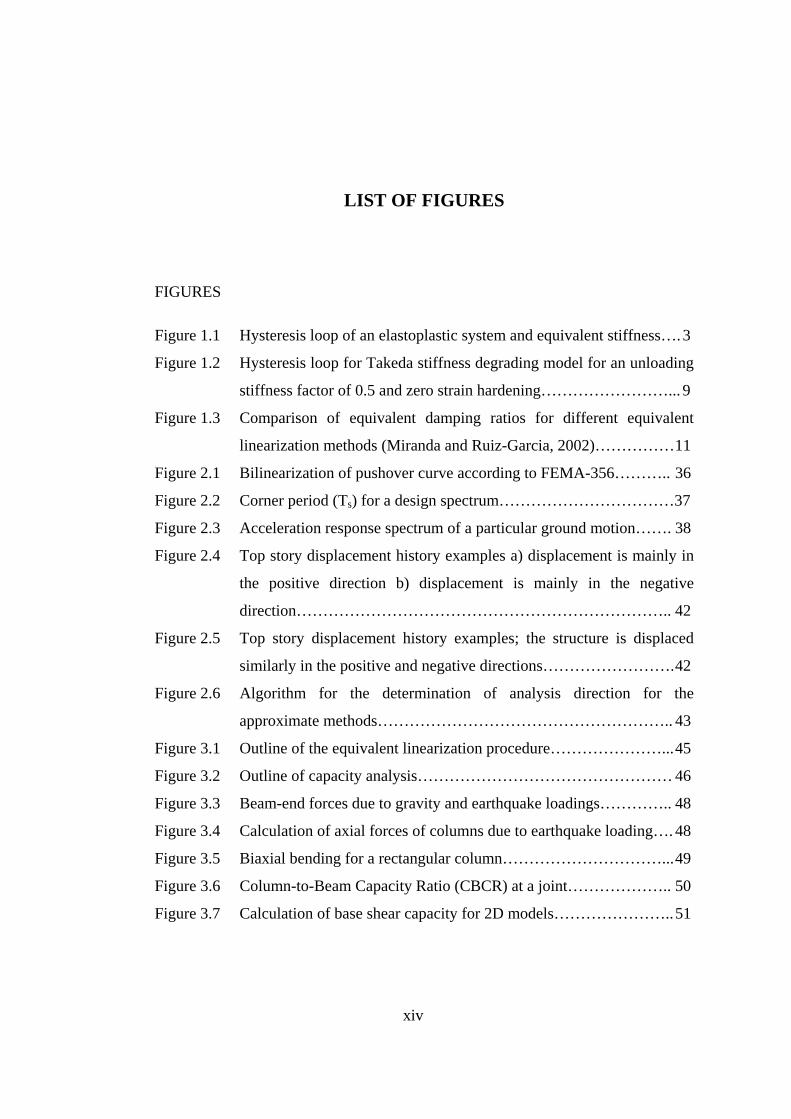
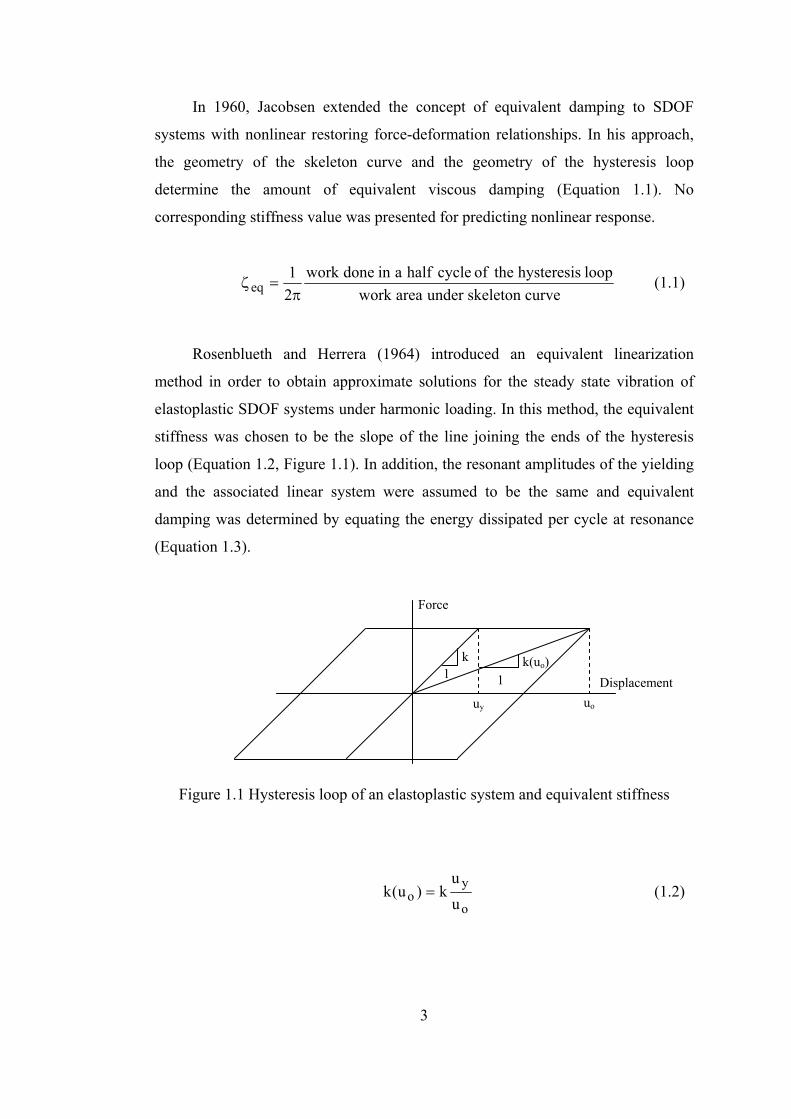
Rosenblueth and Herrera (1964) introduced an equivalent linearization
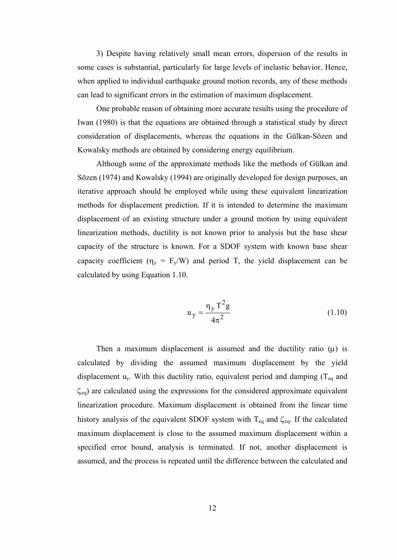
method in order to obtain approximate solutions for the steady state vibration of
elastoplastic SDOF systems under harmonic loading. In this method, the equivalent
stiffness was chosen to be the slope of the line joining the ends of the hysteresis
loop (Equation 1.2, Figure 1.1). In addition, the resonant amplitudes of the yielding
and the associated linear system were assumed to be the same and equivalent
damping was determined by equating the energy dissipated per cycle at resonance
(Equation 1.3).
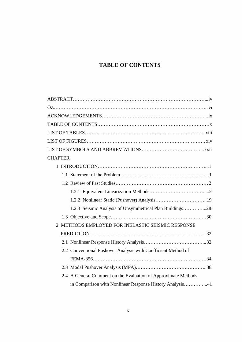
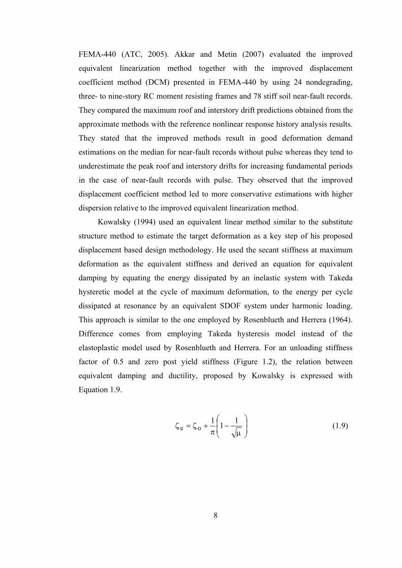
Figure 1.1 Hysteresis loop of an elastoplastic system and equivalent stiffness
o
yo u
uk)u(k = (1.2)
uo uy
k 1
k(uo) 1
Force
Displacement
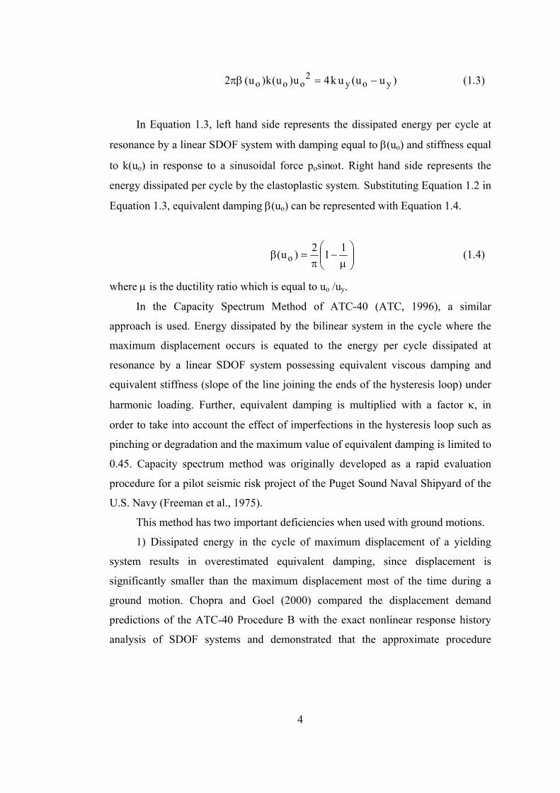
4
)uu(uk4u)u(k)u(2 yoy2
ooo −=πβ (1.3)
In Equation 1.3, left hand side represents the dissipated energy per cycle at
resonance by a linear SDOF system with damping equal to β(uo) and stiffness equal
to k(uo) in response to a sinusoidal force posinωt. Right hand side represents the
energy dissipated per cycle by the elastoplastic system. Substituting Equation 1.2 in
Equation 1.3, equivalent damping β(uo) can be represented with Equation 1.4.
⎟⎟⎠
⎞⎜⎜⎝
⎛μ
−π
=β112)u( o (1.4)
where μ is the ductility ratio which is equal to uo /uy.
In the Capacity Spectrum Method of ATC-40 (ATC, 1996), a similar
approach is used. Energy dissipated by the bilinear system in the cycle where the
maximum displacement occurs is equated to the energy per cycle dissipated at
resonance by a linear SDOF system possessing equivalent viscous damping and
equivalent stiffness (slope of the line joining the ends of the hysteresis loop) under
harmonic loading. Further, equivalent damping is multiplied with a factor κ, in
order to take into account the effect of imperfections in the hysteresis loop such as
pinching or degradation and the maximum value of equivalent damping is limited to
0.45. Capacity spectrum method was originally developed as a rapid evaluation
procedure for a pilot seismic risk project of the Puget Sound Naval Shipyard of the
U.S. Navy (Freeman et al., 1975).
This method has two important deficiencies when used with ground motions.
1) Dissipated energy in the cycle of maximum displacement of a yielding
system results in overestimated equivalent damping, since displacement is
significantly smaller than the maximum displacement most of the time during a
ground motion. Chopra and Goel (2000) compared the displacement demand
predictions of the ATC-40 Procedure B with the exact nonlinear response history
analysis of SDOF systems and demonstrated that the approximate procedure
5
underestimated the displacements significantly for a wide range of period values
with errors approaching 50%.
2) Dissipated energy per cycle of the linear system is calculated by
considering the response to a harmonic force at resonance, which is not the case
during a ground motion. It can be justifiable if there is a dominant pulse with
frequency close to the equivalent natural frequency, however it is misleading for
ground motions containing significant components from a broad range of
frequencies.
Jennings (1968) examined six different methods in which equivalent viscous
damping can be defined for the steady state response of SDOF elasto-plastic
oscillators to sinusoidal excitation. The methods of Jacobsen (1960) and
Rosenblueth and Herrera (1964) were among the investigated methods. In all
considered methods except the method of Jacobsen, equivalent damping was
calculated by equating the energy per cycle dissipated by the equivalent linear
system at resonance to that dissipated by the yielding system. Different equivalent
damping ratios were obtained in each method due to the differences in the
consideration of stiffness and mass employed in describing the equivalent linear
systems. Jennings stated that any of the considered methods might be appropriate
under certain circumstances; however the method which uses equivalent damping
and the initial stiffness was preferable because of its clarity, simplicity and
conservative results.
Gülkan and Sozen (1974) stated that the response of reinforced concrete
structures to strong earthquake motions was influenced by two basic phenomena,
which were reduction in stiffness and increase in energy dissipation capacity. They
also stated that the maximum dynamic response of reinforced concrete structures,
which can be represented by SDOF systems, can be approximated by linear
response analysis using a reduced stiffness and a substitute damping. Substitute
damping represents the increase in energy dissipation capacity through the use of
Equation 1.5.
6
dtuumdt)u(m2t
0g
t
0
2oo ∫−=⎥
⎦
⎤⎢⎣
⎡∫ωβ
••••
(1.5)
Equation 1.5 is based on the fact that the energy input from a ground motion
is entirely dissipated by a viscous damper which has a damping ratio equal to
substitute damping, βo. ωo is equal to the natural frequency of the system with
reduced stiffness, calculated as the square root of the ratio of maximum absolute
acceleration to maximum absolute displacement.
Gülkan and Sözen conducted dynamic experiments with one story, one bay
frames. They calculated βo values through Equation 1.5 using the test results. In
doing so, they assumed that the velocity of the equivalent linear system is equal to
the velocity obtained from the test frames. In addition, they calculated ductility ratio
(μ) as the ratio of maximum absolute displacement to calculated yield displacement
using the test results. Utilizing the βo and μ pairs that they have obtained, they
ended up with a relation between βo and μ (Equation 1.6).
⎟⎟⎠
⎞⎜⎜⎝
⎛
μ−+=β
112.002.0o (1.6)
It can be observed from Equation 1.6 that 0.02 is the value of damping ratio
corresponding to no inelasticity.
Gülkan and Sözen expressed that the equivalent viscous damping approach
had considerable potential as a vehicle to interpret the response of RC systems from
the design point of view, and used the equivalent damping approach to estimate the
design base shear corresponding to an assumed displacement limit.
Iwan and Gates (1979) have conducted a statistical study in order to estimate
the effective period and effective damping by using nonlinear SDOF systems
possessing force-deformation relations with nondegrading and degrading properties.
They used twelve ground motions representing a variety of different types of
earthquake excitation. They calculated the spectral displacements corresponding to
7
different ductility levels considering nine period values. Then they tried to minimize
the differences between these displacements and the displacements obtained by
conducting elastic analyses of SDOF systems with shifted periods and effective
damping values. They observed that the period shift is always less than an order of
two even for very large ductility and the optimum effective damping never exceeds
14% for all the systems that they have analyzed. They also observed that the
primary effect of deterioration or stiffness degradation is to increase the effective
period but they do not have a significant effect on effective damping.
Using the optimum effective period and damping values of Iwan and Gates,
Iwan (1980) developed the empirical relations represented by Equations 1.7 and 1.8
for effective period and effective damping in the period range of 0.4 -4.0 s and for
ductility ratios in the range of 2 to 8.
939.0oe )1(121.01TT −μ+= (1.7)
371.0oe )1(0587.0 −μ=ζ−ζ (1.8)
In Equations 1.7 and 1.8, Te is the effective period, ζe is the effective damping
ratio, To is the initial period, ζo is the damping ratio corresponding to no inelasticity,
and μ is the ductility ratio.
Iwan observed that the differences in hysteretic behavior have a secondary
effect on the accuracy of results predicted by his empirical equations. He compared
the response predictions of the empirical equations, with the predictions of
Newmark-Hall method (1973), substitute structure method (Shibata and Sozen,
1976) and ATC-3 (1978) design guidelines, and concluded that his empirical
equations seem to produce more accurate predictions than those produced by the
other considered methods.
A more comprehensive version of the optimization study of Iwan (1980) was
conducted by Guyader (2003) to obtain equations for the effective damping and
effective period values of bilinear, stiffness degrading and strength degrading
SDOF systems for use in an improved equivalent linearization procedure in
8
FEMA-440 (ATC, 2005). Akkar and Metin (2007) evaluated the improved
equivalent linearization method together with the improved displacement
coefficient method (DCM) presented in FEMA-440 by using 24 nondegrading,
three- to nine-story RC moment resisting frames and 78 stiff soil near-fault records.
They compared the maximum roof and interstory drift predictions obtained from the
approximate methods with the reference nonlinear response history analysis results.
They stated that the improved methods result in good deformation demand
estimations on the median for near-fault records without pulse whereas they tend to
underestimate the peak roof and interstory drifts for increasing fundamental periods
in the case of near-fault records with pulse. They observed that the improved
displacement coefficient method led to more conservative estimations with higher
dispersion relative to the improved equivalent linearization method.
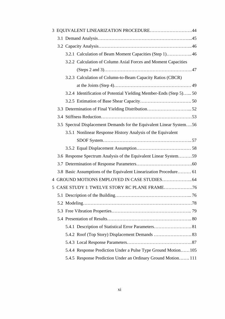
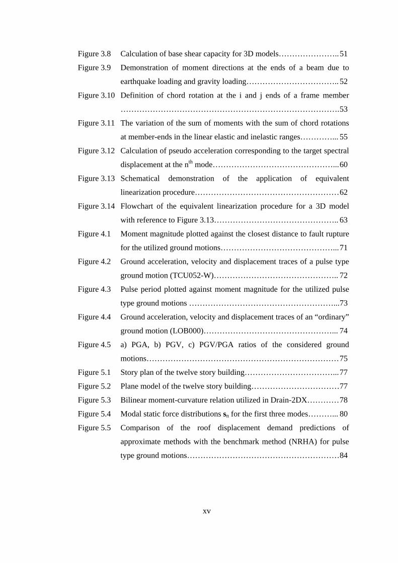
Kowalsky (1994) used an equivalent linear method similar to the substitute
structure method to estimate the target deformation as a key step of his proposed
displacement based design methodology. He used the secant stiffness at maximum
deformation as the equivalent stiffness and derived an equation for equivalent
damping by equating the energy dissipated by an inelastic system with Takeda
hysteretic model at the cycle of maximum deformation, to the energy per cycle
dissipated at resonance by an equivalent SDOF system under harmonic loading.
This approach is similar to the one employed by Rosenblueth and Herrera (1964).
Difference comes from employing Takeda hysteresis model instead of the
elastoplastic model used by Rosenblueth and Herrera. For an unloading stiffness
factor of 0.5 and zero post yield stiffness (Figure 1.2), the relation between
equivalent damping and ductility, proposed by Kowalsky is expressed with
Equation 1.9.
⎟⎟⎠
⎞⎜⎜⎝
⎛
μ−
π+ζ=ζ
111oe (1.9)
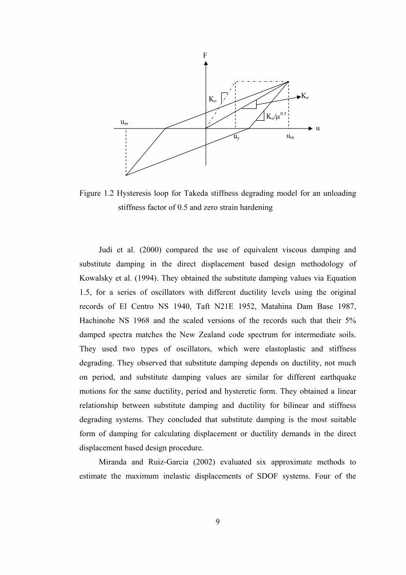
9
Figure 1.2 Hysteresis loop for Takeda stiffness degrading model for an unloading
stiffness factor of 0.5 and zero strain hardening
Judi et al. (2000) compared the use of equivalent viscous damping and
substitute damping in the direct displacement based design methodology of
Kowalsky et al. (1994). They obtained the substitute damping values via Equation
1.5, for a series of oscillators with different ductility levels using the original
records of El Centro NS 1940, Taft N21E 1952, Matahina Dam Base 1987,
Hachinohe NS 1968 and the scaled versions of the records such that their 5%
damped spectra matches the New Zealand code spectrum for intermediate soils.
They used two types of oscillators, which were elastoplastic and stiffness
degrading. They observed that substitute damping depends on ductility, not much
on period, and substitute damping values are similar for different earthquake
motions for the same ductility, period and hysteretic form. They obtained a linear
relationship between substitute damping and ductility for bilinear and stiffness
degrading systems. They concluded that substitute damping is the most suitable
form of damping for calculating displacement or ductility demands in the direct
displacement based design procedure.
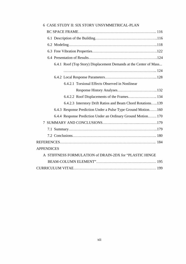
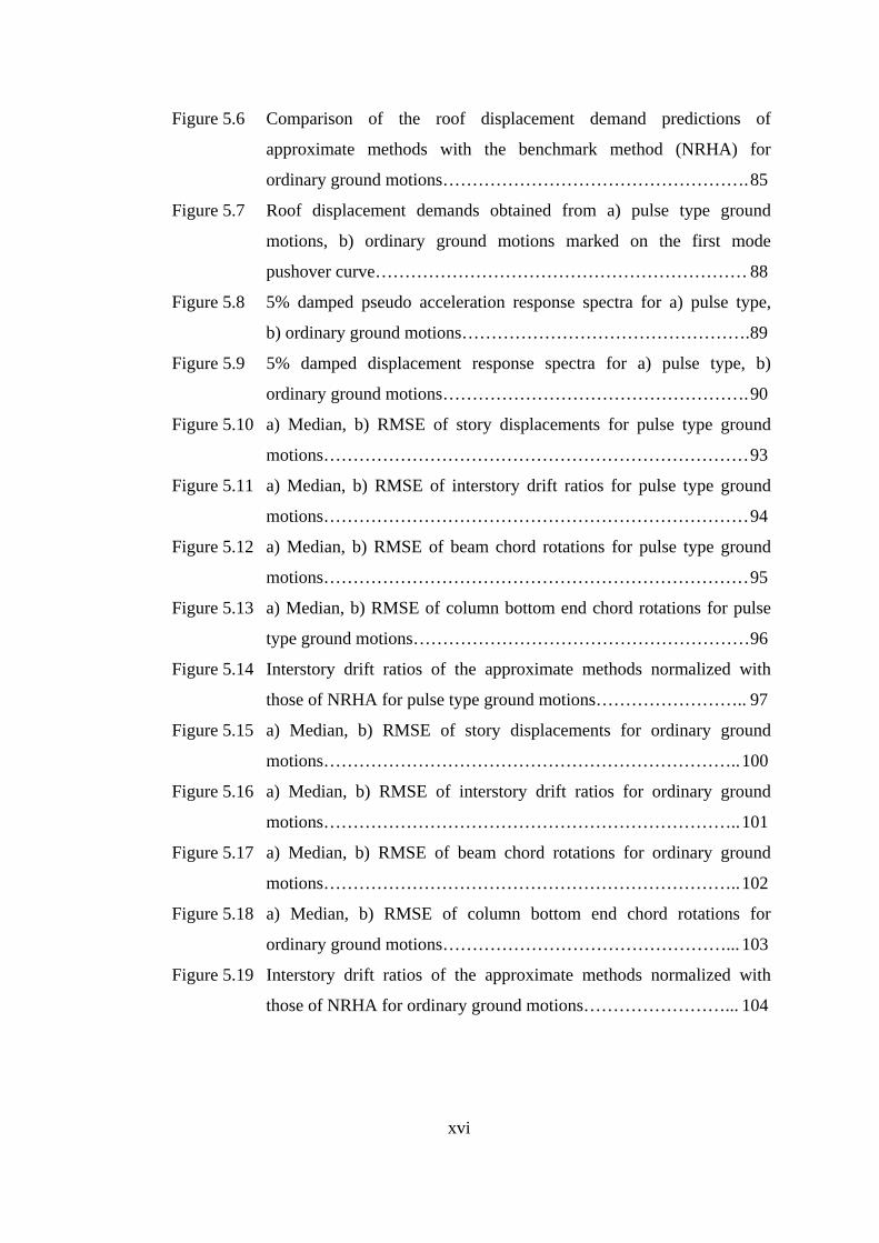
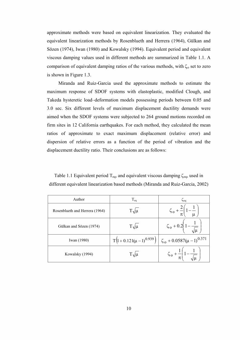
Miranda and Ruiz-Garcia (2002) evaluated six approximate methods to
estimate the maximum inelastic displacements of SDOF systems. Four of the
Ko
Ko/μ0.5
Ke
um
u
uy um
F
10
approximate methods were based on equivalent linearization. They evaluated the
equivalent linearization methods by Rosenblueth and Herrera (1964), Gülkan and
Sözen (1974), Iwan (1980) and Kowalsky (1994). Equivalent period and equivalent
viscous damping values used in different methods are summarized in Table 1.1. A
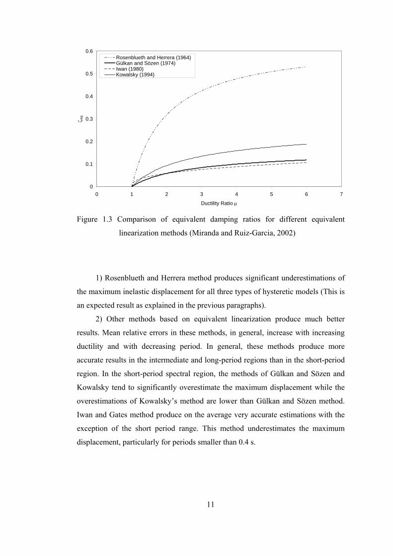
comparison of equivalent damping ratios of the various methods, with ζo set to zero
is shown in Figure 1.3.
Miranda and Ruiz-Garcia used the approximate methods to estimate the
maximum response of SDOF systems with elastoplastic, modified Clough, and
Takeda hysteretic load–deformation models possessing periods between 0.05 and
3.0 sec. Six different levels of maximum displacement ductility demands were
aimed when the SDOF systems were subjected to 264 ground motions recorded on
firm sites in 12 California earthquakes. For each method, they calculated the mean
ratios of approximate to exact maximum displacement (relative error) and
dispersion of relative errors as a function of the period of vibration and the
displacement ductility ratio. Their conclusions are as follows:
Table 1.1 Equivalent period Teq, and equivalent viscous damping ζeq, used in
different equivalent linearization based methods (Miranda and Ruiz-Garcia, 2002)
Author Teq ζeq
Rosenblueth and Herrera (1964) μT ⎟⎟⎠
⎞⎜⎜⎝
⎛μ
−π
+ζ112
o
Gülkan and Sözen (1974) μT ⎟⎟⎠
⎞⎜⎜⎝
⎛
μ−+ζ
112.0o
Iwan (1980) ( )939.0)1(121.01T −μ+ 371.0o )1(0587.0 −μ+ζ
Kowalsky (1994) μT ⎟⎟⎠
⎞⎜⎜⎝
⎛
μ−
π+ζ
111o
11
Figure 1.3 Comparison of equivalent damping ratios for different equivalent
linearization methods (Miranda and Ruiz-Garcia, 2002)
1) Rosenblueth and Herrera method produces significant underestimations of
the maximum inelastic displacement for all three types of hysteretic models (This is
an expected result as explained in the previous paragraphs).
2) Other methods based on equivalent linearization produce much better
results. Mean relative errors in these methods, in general, increase with increasing
ductility and with decreasing period. In general, these methods produce more
accurate results in the intermediate and long-period regions than in the short-period
region. In the short-period spectral region, the methods of Gülkan and Sözen and
Kowalsky tend to significantly overestimate the maximum displacement while the
overestimations of Kowalsky’s method are lower than Gülkan and Sözen method.
Iwan and Gates method produce on the average very accurate estimations with the
exception of the short period range. This method underestimates the maximum
displacement, particularly for periods smaller than 0.4 s.
0
0.1
0.2
0.3
0.4
0.5
0.6
0 1 2 3 4 5 6 7
Ductility Ratio μ
ζ eq
Rosenblueth and Herrera (1964)Gülkan and Sözen (1974)Iwan (1980)Kowalsky (1994)
12
3) Despite having relatively small mean errors, dispersion of the results in
some cases is substantial, particularly for large levels of inelastic behavior. Hence,
when applied to individual earthquake ground motion records, any of these methods
can lead to significant errors in the estimation of maximum displacement.
One probable reason of obtaining more accurate results using the procedure of
Iwan (1980) is that the equations are obtained through a statistical study by direct
consideration of displacements, whereas the equations in the Gülkan-Sözen and
Kowalsky methods are obtained by considering energy equilibrium.
Although some of the approximate methods like the methods of Gülkan and
Sözen (1974) and Kowalsky (1994) are originally developed for design purposes, an
iterative approach should be employed while using these equivalent linearization
methods for displacement prediction. If it is intended to determine the maximum
displacement of an existing structure under a ground motion by using equivalent
linearization methods, ductility is not known prior to analysis but the base shear
capacity of the structure is known. For a SDOF system with known base shear
capacity coefficient (ηy = Fy/W) and period T, the yield displacement can be
calculated by using Equation 1.10.
2
2y
y4
gTu
π
η= (1.10)
Then a maximum displacement is assumed and the ductility ratio (μ) is
calculated by dividing the assumed maximum displacement by the yield
displacement uy. With this ductility ratio, equivalent period and damping (Teq and
ζeq) are calculated using the expressions for the considered approximate equivalent
linearization procedure. Maximum displacement is obtained from the linear time
history analysis of the equivalent SDOF system with Teq and ζeq. If the calculated
maximum displacement is close to the assumed maximum displacement within a
specified error bound, analysis is terminated. If not, another displacement is
assumed, and the process is repeated until the difference between the calculated and
13
the assumed displacements is smaller than the specified error bound. Through such
an analysis, equivalent damping and equivalent period are calculated automatically
at the end of iterations.
In fact, this iterative method is the basis of the procedure presented in the
capacity spectrum method of ATC-40 (ATC, 1996) and the improved equivalent
linearization method developed in FEMA-440 (ATC, 2005), in case that these
methods are employed for use with individual ground motions.
In order to prevent iterations for the calculation of maximum displacements in
the equivalent linearization methods, Miranda and Lin (2004) developed simplified
expressions for equivalent period and equivalent damping ratio as a function of
strength ratio, R and the period of vibration, T (Equations 1.11 and 1.12). In the
derivation of these expressions, they tried to minimize the error between the exact
maximum nonlinear displacement and the approximate displacement obtained by
using equivalent damping and period. They conducted analyses for 72 ground
motions, seven levels of force reduction factors and 48 periods of vibration. They
used an initial viscous damping ratio of 5% in their analyses.
( ) ⎟⎟⎠
⎞⎜⎜⎝
⎛+−+= 6.1
8.1eq
T01.0027.01R1
TT
(1.11)
( ) ⎟⎟⎠
⎞⎜⎜⎝
⎛+−+ζ=ζ 4.2oeq
T002.002.01R (1.12)
Akkar and Miranda (2005) evaluated the accuracy of five approximate
methods in estimating the maximum displacement demand of single degree of
freedom systems possessing elastoplastic force-deformation relations by utilizing
216 ground motions recorded in firm sites during 12 California earthquakes. Three
of the evaluated methods were based on equivalent linearization. They evaluated the
equivalent linearization methods of Iwan (1980), Kowalsky (1994) and Guyader
(2003). With regard to the above discussion about the application of equivalent
linearization methods based on ductility ratios (μ), they used the single degree of
14
freedom systems with known lateral strengths instead of ductility ratios. They
observed that all of the considered equivalent linearization methods have a tendency
to overestimate the deformation demands for systems in the short period range
(T<0.5 sec). The method of Kowalsky overestimated the response for periods
longer than 1.0 sec. According to the results of their study, they concluded that the
users of nonlinear static procedures where target displacements are calculated using
equivalent linear methods or displacement modification factors should be aware of
the limited accuracy provided by these methods, especially for stiff systems with
low lateral strengths in the period range smaller than 0.6 sec.
b) MDOF Systems
In literature, the number of studies related to the application of equivalent
linearization methods to MDOF systems is much less than the number of studies
related to the application of equivalent linearization methods to SDOF systems.
Schnabel et al. (1972) developed the computer program SHAKE for seismic
response analysis of soil layers based on one-dimensional wave propagation. The
nonlinearity of the shear modulus and damping were accounted for by employing
equivalent linear soil properties (Idriss and Seed, 1968; Seed and Idriss, 1970). An
iterative procedure was implemented in order to obtain the equivalent linear values
for shear modulus and damping compatible with the effective strains in each layer.
Outline of the method is as follows.
1. Initial estimates of G (shear modulus) and damping (ζ) are made for each
layer.
2. Using the estimated G and ζ values, linear analysis is conducted to
compute the ground response and maximum shear strain for each layer.
The effective shear strain is determined as a percentage of the maximum
shear strain.
3. New equivalent linear values of G and ζ corresponding to the calculated
effective shear strain values are determined.
15
4. Steps 2 and 3 are repeated until differences between the computed shear
modulus and damping ratios in two successive iterations fall below a
predetermined value in all layers.
Mengi et al. (1992) employed a similar approach for the equivalent linear
earthquake analysis of brick masonry buildings.
Shibata and Sözen (1976) used the idea of employing equivalent stiffness and
damping in their substitute structure method. The substitute structure method is a
design method which is used to determine the minimum strengths of the elements of
a structure such that a tolerable response displacement is not likely to be exceeded.
They indicated that the structure should satisfy the following conditions in order to
apply the substitute structure method.
• The system can be analyzed in a single vertical plane.
• There exists no abrupt change in geometry and mass along the height of
the structure.
• Beams, columns and walls may be designed for different limits of
inelastic response, but all beams in the same bay or all columns in the
same axis should have the same limit.
• Elements and joints are designed and reinforced to avoid significant
strength decay as a result of inelastic response.
• Non-structural elements do not interfere with response.
In addition to the assumptions stated above, it is observed that the method is
applicable when the failure mode of the members is bending and brittle shear
failures do not exist. Since the substitute structure method is a design method, it is
obvious that shear failures should be prevented.
In the substitute structure method, stiffness of the structure is reduced by
reducing the stiffness of elements. Stiffness of element i of the substitute structure is
obtained from Equation 1.13.
i
aisi
)EI()EI(
μ= (1.13)
16
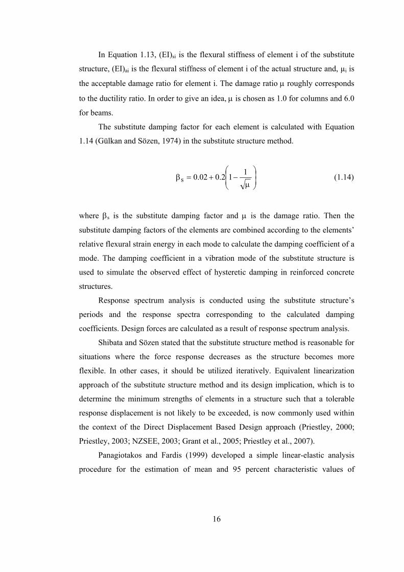
In Equation 1.13, (EI)si is the flexural stiffness of element i of the substitute
structure, (EI)ai is the flexural stiffness of element i of the actual structure and, µi is
the acceptable damage ratio for element i. The damage ratio μ roughly corresponds
to the ductility ratio. In order to give an idea, μ is chosen as 1.0 for columns and 6.0
for beams.
The substitute damping factor for each element is calculated with Equation
1.14 (Gülkan and Sözen, 1974) in the substitute structure method.
⎟⎟⎠
⎞⎜⎜⎝
⎛
μ−+=β
112.002.0s (1.14)
where βs is the substitute damping factor and μ is the damage ratio. Then the
substitute damping factors of the elements are combined according to the elements’
relative flexural strain energy in each mode to calculate the damping coefficient of a
mode. The damping coefficient in a vibration mode of the substitute structure is
used to simulate the observed effect of hysteretic damping in reinforced concrete
structures.
Response spectrum analysis is conducted using the substitute structure’s
periods and the response spectra corresponding to the calculated damping
coefficients. Design forces are calculated as a result of response spectrum analysis.
Shibata and Sözen stated that the substitute structure method is reasonable for
situations where the force response decreases as the structure becomes more
flexible. In other cases, it should be utilized iteratively. Equivalent linearization
approach of the substitute structure method and its design implication, which is to
determine the minimum strengths of elements in a structure such that a tolerable
response displacement is not likely to be exceeded, is now commonly used within
the context of the Direct Displacement Based Design approach (Priestley, 2000;
Priestley, 2003; NZSEE, 2003; Grant et al., 2005; Priestley et al., 2007).
Panagiotakos and Fardis (1999) developed a simple linear-elastic analysis
procedure for the estimation of mean and 95 percent characteristic values of
17
inelastic chord rotation demands in the individual members of multistory RC frame
buildings which are symmetric in plan. They benefited from the equal displacement
rule, since the cracked fundamental periods of the considered elastic structures are
usually beyond the corner periods of the ground motions. They stated that the
fundamental periods of even low-rise bare RC structures are normally longer than
the predominant or corner period of the ground motions which cause full cracking
and bring several members to incipient yielding, as evidenced by full-scale
pseudodynamic or shake table tests. They employed the chord rotation demands,
which they regarded as the most meaningful deformation measure for the
assessment or proportioning of RC members, as the deformation demand parameter.
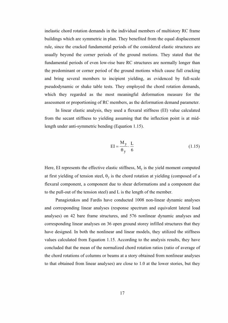
In linear elastic analysis, they used a flexural stiffness (EI) value calculated
from the secant stiffness to yielding assuming that the inflection point is at mid-
length under anti-symmetric bending (Equation 1.15).
6LM
EIy
y ⋅θ
= (1.15)
Here, EI represents the effective elastic stiffness, My is the yield moment computed
at first yielding of tension steel, θy is the chord rotation at yielding (composed of a
flexural component, a component due to shear deformations and a component due
to the pull-out of the tension steel) and L is the length of the member.
Panagiotakos and Fardis have conducted 1008 non-linear dynamic analyses
and corresponding linear analyses (response spectrum and equivalent lateral load
analyses) on 42 bare frame structures, and 576 nonlinear dynamic analyses and
corresponding linear analyses on 36 open ground storey infilled structures that they
have designed. In both the nonlinear and linear models, they utilized the stiffness
values calculated from Equation 1.15. According to the analysis results, they have
concluded that the mean of the normalized chord rotation ratios (ratio of average of
the chord rotations of columns or beams at a story obtained from nonlinear analyses
to that obtained from linear analyses) are close to 1.0 at the lower stories, but they
18
increase at the upper stories where the inelastic deformations are not as important as
the lower stories. They also concluded that the use of multimodal response
spectrum analysis estimated the inelastic chord rotations better than the equivalent
static lateral load analysis.
Kosmopoulos and Fardis (2007) tested the approach of Panagiotakos and
Fardis for asymmetric RC buildings. For this purpose, they utilized four real
buildings with three to six stories, strong irregularities in plan and little engineered
earthquake resistance and 56 bidirectional smooth-spectra-compatible ground
motions. They observed that for multistorey RC buildings which typically have
fundamental periods in the velocity-sensitive part of the spectrum, 5% damped
linear elastic response spectrum analysis gives unbiased and fairly accurate
estimates of member inelastic chord rotations on average.
According to Part 3 of Eurocode 8 (2005), linear elastic analysis with secant
stiffness is applicable, if the inelasticity distribution over the entire structure is
fairly uniform. For this purpose, flexural demand-to-capacity ratios (analysis
moment/capacity moment) are used. Linear elastic analysis with secant stiffness is
applicable if the maximum DCR value in all primary elements is smaller than 2.5
times the minimum DCR over all primary elements having DCR greater than 1.0.
Kosmopoulos and Fardis applied linear elastic analysis to buildings in which this
criterion was not satisfied. They obtained accurate chord rotation estimations in
comparison with nonlinear response history analyses. They concluded that these
criteria should be reexamined and possibly relaxed to allow wider use of linear
elastic analysis for the estimation of member deformation demands.
Fardis and Kosmopoulos (2007) validated the nonlinear response history
analysis according to Eurocode-8 by comparing its predictions with the
pseudodynamic test results of the SPEAR frame (Kosmopoulos and Fardis, 2004;
Negro et al., 2004). They found good agreement for the floor displacement histories
and member damage. By doing so, they have also showed the validity of the
nonlinear response history analysis as the reference analysis in comparison with
linear elastic analysis.
19
1.2.2 Nonlinear Static (Pushover) Analysis
Saiidi and Sözen (1981) pioneered the idea of nonlinear static analysis (or
pushover) in order to determine the force-deformation characteristics of the SDOF
oscillator in the so called Q-model. In this model, force-deformation characteristics
of a SDOF model is obtained from the variation of the top story displacement with
the overturning moment under monotonically increasing forces with a triangular
shape. The variation of the top story displacement with the overturning moment is
established by considering the moment-curvature relationship of the individual
elements. Saiidi and Hudson (1982), Moehle (1984), Moehle and Alarcon (1986)
modified the Q-model and applied it to the analysis of vertically irregular buildings.
In 1987, Fajfar and Fischinger introduced the N2 method as an extension of
the Q-model. The method mainly consists of four steps. In the first step, capacity
curve representing the stiffness, strength and supplied ductility characteristics of the
considered MDOF system is determined by nonlinear static analysis under a
monotonically increasing lateral load vector. In the second step, the capacity curve
is converted to an equivalent SDOF system. In the third step, maximum
displacement demand of the equivalent SDOF system is calculated by carrying out
nonlinear response history analysis of the equivalent SDOF system. In the last step,
the maximum SDOF displacement is converted to the top story displacement of the
MDOF system and details of the structural response (formation of plastic hinges,
inelastic behavior of different structural elements, etc.) at the pushover step
corresponding to this top story displacement are obtained. It is stated that N2
method is applicable for structures oscillating predominantly in a single mode.
The four steps that comprise the N2 method are the main steps involved in the
seismic assessment methods which employ nonlinear static analysis (designated as
the Nonlinear Static Procedure, NSP, FEMA-356, 2000). Different versions of the
first step may be due to the differences in the shape of the lateral load force vector,
examples of which are triangular distribution, uniform distribution or a distribution
proportional to the multiplication of the mass matrix and the first mode shape
(ATC-40, 1996). Fajfar and Gaspersic (1996) used a force distribution proportional
20
to the mass matrix multiplied with an assumed displacement shape. This
displacement shape may be estimated by considering the post yield mechanism of
the structure.
Different approaches are also proposed to convert the capacity curve to the
equivalent SDOF system. The first modal mass and participation factor are utilized
for this purpose in ATC-40, whereas an assumed displacement shape is used for the
conversion by Fajfar and Gaspersic (1996) and Krawinkler and Seneviratna (1998).
Properties of the SDOF systems obtained from ATC-40 and Fajfar and Gaspersic or
Krawinkler and Seneviratna are equivalent to each other if the first mode shape is
utilized as the displacement shape.
In order to calculate the maximum displacement demand of the SDOF system,
the capacity spectrum method (Freeman et al., 1975; ATC-40, 1996), the coefficient
method (FEMA-356, 2000) or the modified versions of these methods (FEMA-440,
2005) may be utilized. Capacity spectrum method is based on equivalent
linearization as explained in the above paragraphs whereas the coefficient method
calculates the inelastic displacement by multiplying the displacement of a linear
elastic SDOF system with several coefficients. Both the capacity spectrum method
and the coefficient method are approximate methods utilized for the determination
of maximum displacements and possess drawbacks (Chopra and Goel, 2000;
Miranda and Akkar, 2002) when used with individual ground motions. Another
method utilized for the determination of maximum displacement of a SDOF system
is the nonlinear response history analysis of the equivalent SDOF system under a
ground motion. In fact, nonlinear response history analysis of a SDOF system is a
simpler task when compared with the nonlinear static analysis of a MDOF system.
Therefore, the basic motivation of the approximate displacement calculation
methods of ATC-40 (1996) and FEMA-356 (2000) and their variants in FEMA-440
(2005) is not developing easily applicable methods, but to develop displacement
demand prediction methods when the ground excitation is expressed by an elastic
design spectrum. Inelastic response spectra developed in the form of R-μ-T
relations (such as Newmark and Hall, 1982, Krawinkler and Nassar, 1992, Miranda
and Bertero, 1994, Vidic et al., 1994) are also employed for the determination of
21
maximum displacements of the equivalent SDOF systems (Fajfar and Gaspersic,
1996, Fajfar, 2000).
Krawinkler and Seneviratna (1998) discussed the applicability of nonlinear
static analysis (pushover) as a seismic performance evaluation tool. According to
Krawinkler and Seneviratna, pushover can be used qualitatively for the
determination of the consequences of strength deterioration of individual elements
on the behavior of structural system, identification of the critical regions in which
the deformation demands are expected to be high, identification of the strength
discontinuities in plan or elevation, and verification of the completeness and
adequacy of load path. It can be used quantitatively to determine the force demands
on potentially brittle elements, estimates of the deformation demands for elements
which deform inelastically, and the interstory drifts.
Krawinkler and Seneviratna stated that the invariant load pattern utilized in
the pushover analysis is valid if the structural response is not severely affected by
higher modes, and if the structure has only a single yielding mechanism. They also
stated that the most critical concern is that the pushover analysis may detect only
the first local mechanism which forms under a ground motion and may not capture
other weaknesses which will form after the dynamic characteristics change with the
formation of the first local mechanism. By comparing the results of nonlinear
response history and pushover analyses for a four story steel frame, they concluded
that pushover analysis provides very good predictions of seismic demands for
regular low-rise structures for which higher mode effects are not of concern and for
which inelasticity is distributed uniformly over the height.
Mwafy and Elnashai (2001) claimed that nonlinear response history analysis
is complex and therefore unsuitable for practical design applications despite the
improvement of the accuracy and efficiency of the computational tools. They stated
that the calculated inelastic dynamic response is quite sensitive to the ground
motion characteristics and accordingly the computational effort increases since a
number of representative ground motions should be selected. They employed
different invariant load patterns for pushover analysis (the code design lateral
pattern, uniform distribution and the force distribution obtained by combining the
22
external modal forces with SRSS). They compared the obtained capacity curves
with those obtained by applying the ground motions with incrementally increased
intensities. They also compared the local responses at the global limit state. They
commented that conventional pushover analysis (with invariant lateral forces) is
more appropriate for low rise and short period frame structures and the
discrepancies between nonlinear static analyses and nonlinear response history
analyses for long period buildings can be overcome by utilizing more than one load
pattern.
The studies which are conducted to improve the conventional (single mode)
pushover analysis may be classified as the studies which utilize the adaptive force
distributions, which consider the higher mode effects and those which employ both
of the above considerations.
Bracci et al. (1997) stated that a predetermined lateral load distribution and a
base shear-top story displacement format is not suitable for structures failing from
midstory mechanisms, and extended the capacity spectrum method to include the
effects of potential midstory mechanisms and a story-by-story performance
evaluation using modal superposition. In this method, the lateral forces at each step
are updated by considering the story shear forces at the previous step along with
Equation 1.16. As a result of pushover analysis, shear force versus drift response at
each story is determined and used to capture potential soft story mechanisms.
⎟⎟
⎠
⎞
⎜⎜
⎝
⎛Δ+⎟
⎟
⎠
⎞
⎜⎜
⎝
⎛−=Δ +
−
−+
j
ji1j
1j
1ji
j
jij1j
i V
FP
V
F
V
FVF (1.16)
In Equation 1.16, i is the story number, j is the analysis step, ΔFij+1 is the
incremental ith story force at step j+1, Vj is the base shear at step j, ΔPj+1 is the
incremental base shear applied at step j+1 and Fij is the ith story force at step j.
Bracci et al. mentioned that dynamic strain rate effects and system
degradation or deterioration are not captured in pushover analysis, since it is based
on the static application of lateral story forces. They commented that these effects
23
could be accounted for by adjusting the moment-curvature properties of the
members. However, they did not present an explicit method on this issue.
Gupta and Kunnath (2000) developed a procedure which considers the
adaptive nature of lateral forces as well as the higher mode effects. They showed
the limitations of conventional static procedures, by utilizing the response of
instrumented buildings which experienced strong ground motions during 1994
Northridge earthquake. For this purpose, they observed the vertical distribution of
inertia forces at the times of maximum displacement, maximum drift, maximum
base shear and maximum overturning moment. They concluded that higher mode
effects significantly affect the response of buildings during ground shaking with the
exception of low rise buildings, and stated that higher mode effects are better
understood by analyzing the inertial force and story drift profiles rather than the
displacement profile. In the light of these observations, they developed a method for
pushover analysis of structures which considers the higher mode effects and
accounts for the force distribution following yielding. In this formulation, response
spectrum analysis is conducted at each step of pushover analysis instead of a static
analysis of the conventional pushover. Required modal properties are obtained from
the eigenvalue analysis of the structure at the considered pushover step. Associated
pseudo accelerations are calculated from the elastic response spectrum as the
pseudo accelerations corresponding to the instantaneous period values. They
applied the method on 4, 8, 12, 16 and 20 story 2D reinforced concrete frames by
utilizing 15 ground motions which do not contain significant pulses. They
considered both code designed frames and the versions of these frames with
strength and stiffness irregularities. They incorporated story drifts and plastic hinge
locations as the response parameters. They showed that uniform and FEMA-273
(ATC, 1997) modal load patterns were inadequate in capturing the response for
high-rise frames where higher mode effects are important, whereas the proposed
method performed reasonably well and resulted in close responses to nonlinear
response history analyses. In the application of this method, they did not state
explicitly the calculation of a global displacement demand at which the response
24
parameters are obtained. They only commented that FEMA-273 coefficient method
could be used for this purpose.
Aydınoğlu (2003) observed that elastic pseudo accelerations corresponding to
the instantaneous periods in Gupta and Kunnath’s method are not compatible with
the inelastic instantaneous response, and modified Gupta and Kunnath’s
incremental response spectrum analysis procedure by considering inelastic spectral
displacements corresponding to the instantaneous state of the system instead of the
elastic pseudo accelerations. He stated that utilization of inelastic spectral
displacements permitted consistent estimation of the peak response quantities at the
last step of pushover analysis, where the analysis ends upon a control process.
Therefore, the top story displacement at the last step is the global displacement
demand. The results obtained for a presented case study were sufficiently close to
the nonlinear response history analysis results, at the expense of considerable
computational work. Aydınoğlu also developed a practical version of his method for
smooth elastic response spectrum by employing the equal displacement rule.
Antoniou and Pinho (2004a) also developed a procedure similar to that of
Gupta and Kunnath (2000) in order to take into consideration the higher mode
effects and variant force distributions. They stated that equilibrium can not be
satisfied at each step of pushover analysis due to the combination rules (such as
SRSS or CQC) utilized for the combination of modal responses in the method of
Gupta and Kunnath. Instead, Antoniou and Pinho combined the external modal
forces using modal combination rules at each step of pushover analysis in order to
determine the lateral forces to be applied at the corresponding step. As an
alternative, they combined the external modal static forces (defined as the external
modal forces divided by the pseudo acceleration, Chopra, 2001). They called the
former and latter methods as the methods “with spectral amplification” and
“without spectral amplification” respectively. They commented that the
combination of the external modal forces should be done by adding them vectorially
for the purpose of a better match with nonlinear dynamic response. However, they
did not investigate the applicability of such an option. In addition to the “with
spectral amplification” and “without spectral amplification” cases, they also
25
employed “total updating” and “incremental updating” alternatives for the lateral
forces to be applied at each step. In the “total updating” alternative, the lateral force
calculated as explained above is applied as the external force, whereas it is added
with proper scaling to the external force at the previous step in the “incremental
updating” alternative. They stated that the method “with spectral amplification” and
“incremental updating” is the most suitable when numerical stability and the
accuracy of the results are observed. They evaluated the proposed method in
comparison with conventional pushover analyses (employing uniform and
triangular distributions) with reference to nonlinear response history analyses, by
conducting a parametric study with regular, irregular and dual systems using 2D
models and four ground motions. They concluded that the proposed adaptive
pushover method features a relatively minor advantage over the conventional
pushover analysis.
In a companion paper, Antoniou and Pinho (2004b) developed a
displacement-based adaptive pushover procedure, in which a displacement vector
updated according to the instantaneous stiffness of the structure is imposed at each
step of the analysis. The displacement vector combines the contributions from all
modes by employing a combination rule. Similar to the companion paper, “with
spectral amplification”, “without spectral amplification”, “incremental updating”
and “total updating” alternatives are utilized. Similar to the force-based case, a
global displacement demand is not calculated in this method. They used the same
frames and ground motions with the companion paper for the validation part. They
concluded that the proposed method provides greatly improved predictions in
comparison to the conventional pushover analysis throughout the entire deformation
range.
Main disadvantage of the methods in which adaptive nature of lateral forces
(or displacements) are taken into consideration (Gupta and Kunnath, 2000;
Aydınoğlu, 2003; Antoniou and Pinho, 2004a, 2004b) is that they are conceptually
complicated and computationally demanding for routine application in structural
engineering practice (Chopra and Goel, 2002). They can not be applied directly by
using the software developed for conventional pushover analysis. Instead, these
26
methods should be implemented in the source codes of the available software. The
methods in which higher mode effects are considered and the adaptive nature of
lateral forces is not taken into consideration are conceptually less complicated and
they can be directly applied by utilizing the available software for conventional
pushover analysis through post-processing.
Paret et al., (1996) introduced the idea of conducting several pushover
analyses with force distributions proportional to the multiplication of the mass
matrix and the elastic mode shapes corresponding to different modes of the
structure. As a result of these analyses, a pushover curve is obtained for each of the
considered modes. Then, the pushover curves are converted into ADRS format
(Mahaney et al., 1993). Pseudo acceleration corresponding to yielding is obtained
from the pushover curves in ADRS format. Then the elastic pseudo acceleration
corresponding to the period of the considered mode is obtained from the utilized
elastic spectrum. Elastic pseudo acceleration is divided by the pseudo acceleration
corresponding to yielding in order to calculate the Modal Criticality Index (MCI)
for each mode and the critical mode is determined as the mode with highest MCI.
The procedure is applied graphically in order to preserve the graphical
attractiveness of the capacity spectrum method.
Sasaki et al. (1998) extended the idea of MCI to identify the failure modes in
the Multi-Mode Pushover (MMP) procedure. They did not specify a combination
procedure for modal responses.
Chopra and Goel (2002) improved the MMP procedure to develop Modal
Pushover Analysis (MPA). A pushover analysis is conducted under an invariant
load pattern for each mode independently, and then inelastic modal demands are
calculated by independent nonlinear response history analysis of the equivalent
inelastic SDOF systems which are represented by the associated modal capacity
curves. Finally, modal response quantities are combined with SRSS or CQC as in
response spectrum analysis (RSA). MPA fully reduces to RSA in case of linear
elastic response. Implementation of MPA is simple and requires only a post-
processing effort. Its major drawback is the assumption of independent inelastic
response at each mode, which is not theoretically correct. While this assumption
27
leads to acceptable results for lower order response quantities (displacement, drift),
it usually leads to errors for higher order response quantities (plastic rotations,
curvatures, etc.). Chintanapakdee and Chopra (2003) evaluated the accuracy of
MPA by utilizing height-wise regular generic frames. Goel and Chopra (2004)
improved MPA, especially in its treatment of P–Δ effects due to gravity loads and
calculation of plastic hinge rotations. Chintanapakdee and Chopra (2004) evaluated
the accuracy of MPA by using vertically irregular generic frames. Chopra et al.
(2004) proposed a modified version of MPA (MMPA) in which the inelastic
response obtained from first-mode pushover analysis has been combined with the
elastic contribution of higher modes. Chopra and Goel (2004) presented the
application of MPA to buildings with unsymmetrical plan.
Kalkan and Kunnath (2006) proposed a pushover analysis procedure which is
derived through adaptive modal combinations (AMC). This method attempts to
integrate concepts built into the capacity spectrum method (ATC-40, 1996), the
adaptive method proposed by Gupta and Kunnath (2000) and the modal pushover
analysis of Chopra and Goel (2002).
Relying on nonlinear response history analyses, Vamvatsikos and Cornell
(2002) developed the (single-record) incremental dynamic analysis procedure (IDA)
for generating intensity-demand diagrams similar to pushover capacity curves,
where variations in structural response under a specific ground motion record is
fully accounted for. Generation of a single IDA curve requires several nonlinear
response history analysis of the structural system under scaled ground motions.
Recently, Aschheim et al. (2007) proposed a scaled nonlinear dynamic procedure
(NDP) for improving nonlinear static procedures (NSP). Several nonlinear response
history analyses of the investigated structural system are carried out under scaled
ground motions to match the target demand determined from NSP. The obtained
results are then evaluated statistically in order to establish levels of confidence for
the considered response parameters. IDA and scaled NDP may bring new sights
into NSP; however they completely remove its physical and computational
simplicity.
28
1.2.3 Seismic Analysis of Unsymmetrical Plan Buildings
A review of the studies on the seismic response of asymmetric structures
conducted before 1994, between 1994 and 1998 and between 1998 and 2002 were
summarized by Rutenberg et al. (1995), Rutenberg (1998) and Rutenberg (2002),
respectively. Most of the reviewed studies were conducted using simple single-
storey asymmetric models. Summary of the research between the years 2002 and
2007 can be found in De Stefano and Pintucchi (2007). Some of these studies are
also reviewed here.
In the first applications of nonlinear static analysis on 3D unsymmetrical plan
buildings, exact 3D formulations were not utilized. Approximate analysis
procedures were developed. Kilar and Fajfar (1997) described an application of
pushover analysis to asymmetric buildings by modeling the structure as a collection
of planar macro-elements. An approximate relation between the global base shear of
the building and its top displacement is obtained at the end of pushover analysis.
Moghadam and Tso (1998) developed a pushover analysis procedure for
asymmetrical multistory buildings which take into account the higher modal and
three dimensional effects induced by torsion. In this procedure, pushover analysis is
conducted separately for each frame using lateral force distributions obtained from
the elastic response spectrum analysis. Target displacement for each frame is also
obtained from elastic response spectrum analysis. They applied the procedure on a
seven-storey symmetrical plan reinforced concrete building and mass and stiffness
eccentric versions of this building. They conducted reference nonlinear response
history analyses by applying ten artificial ground motions unidirectionally. By
comparison of the floor displacements, interstory drifts and column and beam
ductility demands, they have stated that the proposed method led to good estimates
at the stiff and flexible edge frames of both mass and stiffness eccentric buildings.
Chopra and Goel (2004) extended the application of MPA (Chopra and Goel,
2002) to buildings with unsymmetrical plan. Essentially the procedure is the same
as the 2D case where the torques and the lateral forces in both orthogonal directions
are considered in the external modal force vectors for the 3D case. In the presence
29
of asymmetry about both of the orthogonal axes, there exist two pushover curves.
The authors suggested that the pushover curve in the dominant direction of the
mode should be utilized in such cases. When there is asymmetry about only one of
the axes; such a problem does not occur since there exists a pushover curve only in
one direction. They modified a 9-story symmetric plan steel frame to create a mass
eccentric system. The eccentricity between the center of mass and center of stiffness
was set as 10% of the plan dimension. They further created three versions of the
mass eccentric system by changing the moment of inertia values, which were a
‘torsionally stiff’ system, a ‘torsionally flexible’ system and a ‘torsionally-similarly-
stiff’ system. Periods corresponding to the torsional modes of vibration are
significantly smaller than, significantly greater than and similar to those
corresponding to the translational modes in the torsionally stiff, torsionally flexible
and torsionally-similarly-stiff systems respectively. They applied the method on the
considered buildings by utilizing one ground motion in comparison with nonlinear
response history analysis, and obtained accurate results at the center of mass for
torsionally stiff and torsionally flexible systems. However, erroneous results were
obtained for the torsionally-similarly-stiff system because of the strong coupling of
modes and the underestimation of the roof displacement because of the CQC rule.
They concluded that the application of MPA on unsymmetrical-plan buildings
should be investigated by utilizing an ensemble of ground motions.
Fajfar et al. (2005) performed parametric studies on single and multistory
buildings with bi-axial eccentricity subjected to bi-directional ground motion to
investigate the effect of torsion in the elastic and inelastic ranges of deformation.
They utilized the ratio of the roof displacements at the edge frames to the roof
displacement at the center of mass as the investigated parameter for observing the
effect of torsion. They observed that the torsional effects generally decrease with
increasing inelasticity and stated that the linear elastic response spectrum analysis
results in an upper bound for the torsional effects. Based on these observations, they
extended the N2 method for use in asymmetric buildings. According to this
extension, N2 method applicable to the symmetric systems is employed first. Then
the responses are amplified using the response spectrum analysis results for the
30
consideration of torsion effects. As the amplification factor, the ratio between
normalized roof displacement (roof displacement at an arbitrary location to the roof
displacement at the center of mass) obtained from elastic modal analysis to that
obtained from pushover analysis is used. Minimum value of the amplification factor
is taken as 1.
It can be concluded that the improved pushover methods summarized in the
previous section are generally validated by using 2D frames, but none of them has
been totally validated for 3D unsymmetrical plan buildings.
1.3 Objective and Scope
An equivalent linearization procedure which utilizes the familiar response
spectrum analysis as the analysis tool and benefits from the capacity principles is
presented for the inelastic seismic displacement response prediction of MDOF
systems. The procedure is applied on a twelve story reinforced concrete plane frame
for which higher mode effects are important, and a six story unsymmetrical-plan
reinforced concrete space frame where torsion significantly effects the response.
The predictions of the equivalent linearization procedure are compared with the
nonlinear response history analysis results by utilizing 162 ground motions.
Response predictions from two other approximate procedures, which are
conventional pushover analysis according to FEMA-356 (ASCE, 2000) and modal
pushover analysis (MPA, Chopra and Goel, 2002) are also presented. In addition,
results of response spectrum analyses and linear response history analyses are used
for comparison purposes. Roof displacement demands and several local response
parameters; namely story displacements, interstory drift ratios and chord rotations
are used in the comparative evaluations.
Main objective of the study is to develop an equivalent linearization
procedure for inelastic seismic response prediction of MDOF systems. A
subsequent objective is to test the accuracy of the proposed procedure in predicting
31
the global displacement demands (roof displacements) and local response
parameters.
This thesis is composed of seven main chapters and an appendix. Brief
contents are given as follows:
Chapter 1 Statement of the problem and literature survey on equivalent
linearization methods, pushover analysis and seismic analysis of
unsymmetrical plan buildings.
Chapter 2 Brief information on the inelastic analysis methods employed for
comparing the results obtained from the proposed equivalent
linearization procedure.
Chapter 3 Explanation of the equivalent linearization procedure.
Chapter 4 Information about the employed ground motions.
Chapter 5 Case study I: Twelve story reinforced concrete plane frame.
Application of the equivalent linearization procedure and
comparison of results with those of nonlinear response history
analysis and other approximate methods.
Chapter 6 Case study II: Six story unsymmetrical-plan reinforced concrete
space frame. Application of the equivalent linearization procedure
and comparison of results with those of nonlinear response history
analysis and other approximate methods.
Chapter 7 A brief summary and conclusions.
Appendix A Stiffness formulation of Drain-2DX for “Plastic Hinge Beam-
Column Element”.
32
CHAPTER 2
METHODS EMPLOYED FOR INELASTIC SEISMIC
RESPONSE PREDICTION
The response parameters obtained from the implementation of the proposed
equivalent linearization procedure are compared with those of nonlinear response
history analyses. Moreover, two other approximate methods are also employed in
order to observe the relative accuracy of the predictions of the equivalent
linearization procedure with respect to other approximate methods. One of these
approximate methods is the conventional pushover analysis with the coefficient
method (FEMA-356, ASCE, 2000). The second approximate method is the Modal
Pushover Analysis (MPA) developed by Chopra and Goel (2002). Nonlinear
response history analysis (NRHA), pushover analysis with coefficient method
(PO-FEMA) and MPA are described briefly in the following sections.
2.1 Nonlinear Response History Analysis
Nonlinear response history analysis is accepted as the most accurate
simulation of dynamic response under a ground excitation. In this analysis, the
equation of motion defined with Equation 2.1 is solved in the range of the requested
time interval.
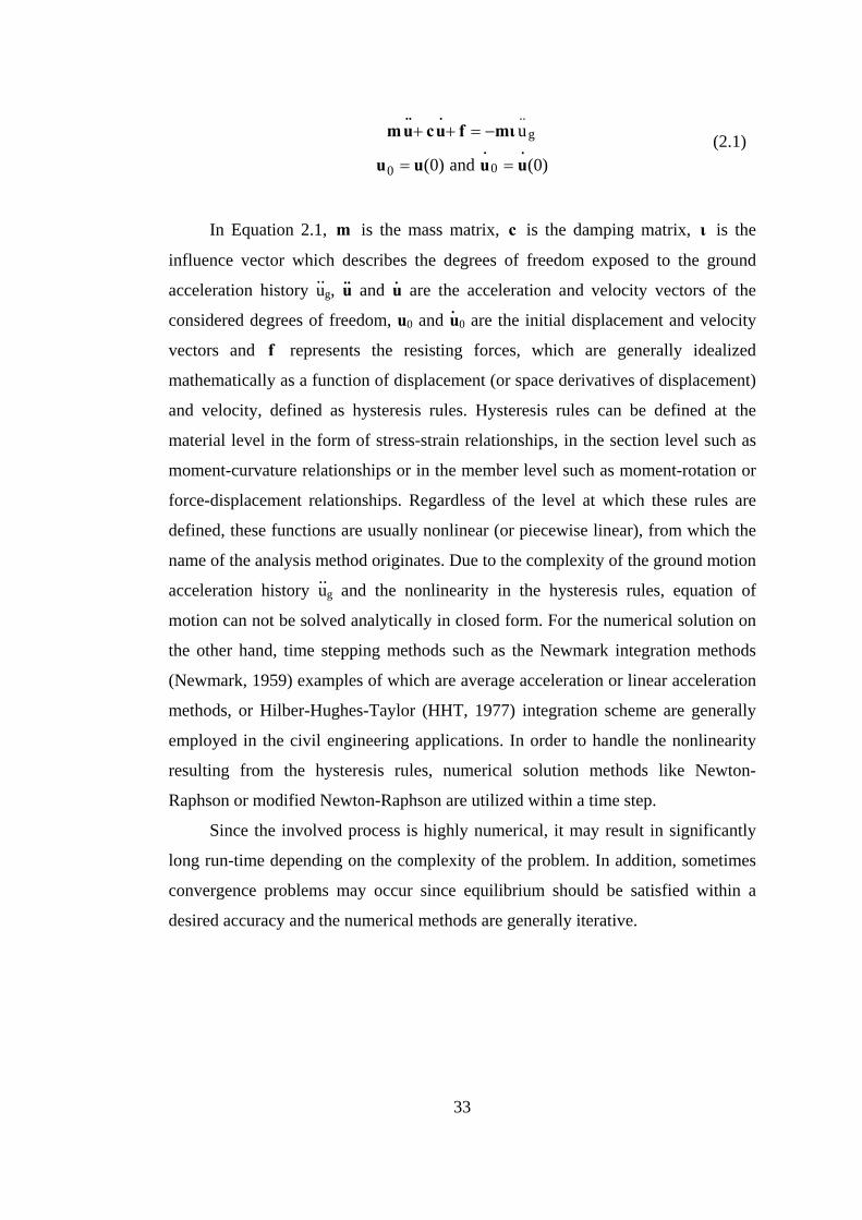
33
)0(and)0(
u
00
g..
..
...
uuuu
mιfucum
==
−=++ (2.1)
In Equation 2.1, m is the mass matrix, c is the damping matrix, ι is the
influence vector which describes the degrees of freedom exposed to the ground
acceleration history ug, u and u are the acceleration and velocity vectors of the
considered degrees of freedom, u0 and u0 are the initial displacement and velocity
vectors and f represents the resisting forces, which are generally idealized
mathematically as a function of displacement (or space derivatives of displacement)
and velocity, defined as hysteresis rules. Hysteresis rules can be defined at the
material level in the form of stress-strain relationships, in the section level such as
moment-curvature relationships or in the member level such as moment-rotation or
force-displacement relationships. Regardless of the level at which these rules are
defined, these functions are usually nonlinear (or piecewise linear), from which the
name of the analysis method originates. Due to the complexity of the ground motion
acceleration history ug and the nonlinearity in the hysteresis rules, equation of
motion can not be solved analytically in closed form. For the numerical solution on
the other hand, time stepping methods such as the Newmark integration methods
(Newmark, 1959) examples of which are average acceleration or linear acceleration
methods, or Hilber-Hughes-Taylor (HHT, 1977) integration scheme are generally
employed in the civil engineering applications. In order to handle the nonlinearity
resulting from the hysteresis rules, numerical solution methods like Newton-
Raphson or modified Newton-Raphson are utilized within a time step.
Since the involved process is highly numerical, it may result in significantly
long run-time depending on the complexity of the problem. In addition, sometimes
convergence problems may occur since equilibrium should be satisfied within a
desired accuracy and the numerical methods are generally iterative.
.. .. .
.
..
34
2.2 Conventional Pushover Analysis with Coefficient Method of FEMA-356
It has long been recognized that damage control should be achieved through
the control of displacements (Shibata and Sözen, 1976). It has also been recognized
that nonlinear analysis should be used for the determination of displacements
(Saiidi and Sözen, 1981; Fajfar and Fishinger, 1987). After the destructive
earthquakes in the last two decades, it has been accepted that nonlinear analysis
should be more explicitly considered for design purposes (Fajfar, 2000). Due to the
above mentioned complexities and difficulties of nonlinear response history
analyses, it would be an impractical decision to enforce the application of nonlinear
response history analyses. Therefore, research has been focused on the simpler
approximate nonlinear analysis methods. Nonlinear static (pushover) analysis has
gained considerable acceptance and popularity as a fairly simple approximate
method.
In conventional pushover analysis, the structure is loaded under gravity
forces, then the lateral forces described by a predetermined distribution is increased
until a specified displacement is achieved, or the structure reaches a collapse state.
The response parameters are recorded in every pushover step. Pushover analysis is
generally represented by a pushover or capacity curve, which is the base shear
plotted against the lateral displacement of a control node. Different lateral load
patterns such as triangular distribution, uniform distribution or a distribution
proportional to the multiplication of the first mode shape and the mass matrix can
be utilized. Latter distribution is used in this study.
Pushover analysis is useful in observing the critical locations where the
deformation demands are expected to be high, identification of the possible strength
discontinuities in plan or elevation and determination of the adequacy of the load
path (Krawinkler and Seneviratna, 1998). It can also be used as a method for the
approximate determination of seismic demands. Such an application of pushover
analysis is presented in FEMA-356 (ASCE, 2000). In this application, a “Target
Displacement” is determined by multiplying the spectral displacement of a linear
elastic single degree of freedom system possessing the effective fundamental period
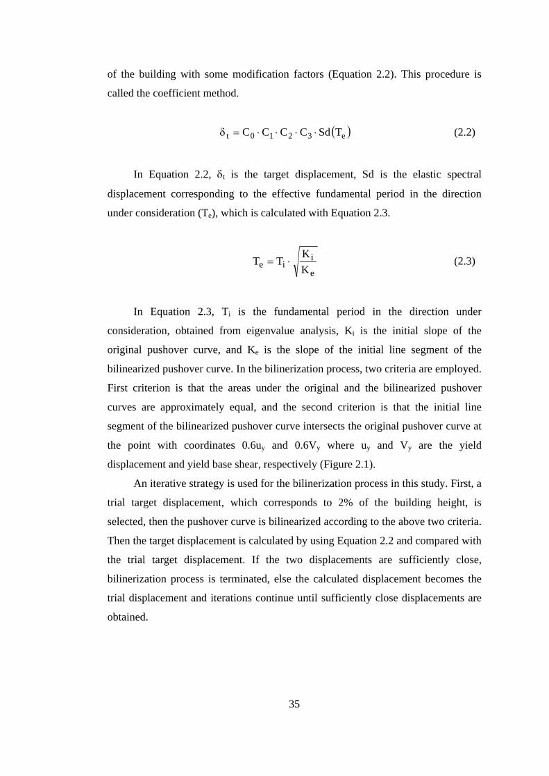
35
of the building with some modification factors (Equation 2.2). This procedure is
called the coefficient method.
( )e3210t TSdCCCC ⋅⋅⋅⋅=δ (2.2)
In Equation 2.2, δt is the target displacement, Sd is the elastic spectral
displacement corresponding to the effective fundamental period in the direction
under consideration (Te), which is calculated with Equation 2.3.
e
iie K
KTT ⋅= (2.3)
In Equation 2.3, Ti is the fundamental period in the direction under
consideration, obtained from eigenvalue analysis, Ki is the initial slope of the
original pushover curve, and Ke is the slope of the initial line segment of the
bilinearized pushover curve. In the bilinerization process, two criteria are employed.
First criterion is that the areas under the original and the bilinearized pushover
curves are approximately equal, and the second criterion is that the initial line
segment of the bilinearized pushover curve intersects the original pushover curve at
the point with coordinates 0.6uy and 0.6Vy where uy and Vy are the yield
displacement and yield base shear, respectively (Figure 2.1).
An iterative strategy is used for the bilinerization process in this study. First, a
trial target displacement, which corresponds to 2% of the building height, is
selected, then the pushover curve is bilinearized according to the above two criteria.
Then the target displacement is calculated by using Equation 2.2 and compared with
the trial target displacement. If the two displacements are sufficiently close,
bilinerization process is terminated, else the calculated displacement becomes the
trial displacement and iterations continue until sufficiently close displacements are
obtained.
36
Figure 2.1 Bilinearization of pushover curve according to FEMA-356
In Equation 2.2, C0, C1, C2 and C3 are the coefficients that modify the elastic
spectral displacement, which are defined below.
C0: Modification factor that relates the SDOF spectral displacement
coordinate to the MDOF system control node displacement.
C1: Modification factor that relates the expected maximum inelastic
displacements to the linear elastic displacements.
C2: Modification factor to represent the effect of pinched hysteretic shape,
stiffness degradation and strength degradation on maximum displacement
response.
C3: Modification factor to represent increased displacements due to P-Δ
effects.
In this study, C0 is defined by the multiplication of first mode participation
factor with the amplitude of the first mode vector at the top story. C1 is calculated
from Equation 2.4, which is presented in FEMA-356. Since stiffness and strength
degradation and P-Δ effects are not considered, C2 and C3 are accepted to be equal
to 1.0.
Bilinearized pushover curve Vy
uy
0.6Vy
0.6uy utarget
Original pushover curve
Approximately equal areas
Base shear
Displacement
37
( )⎩⎨⎧
<−+≥
=sees
se1 TTforTT1R1
TTfor1C
/ (2.4)
where
y
*1
VMSa
R⋅
= (2.5)
In Equations 2.4 and 2.5, Te is the effective fundamental period in the
direction under consideration, Sa is the pseudo acceleration corresponding to Te,
M1* is the effective first modal mass, Vy is the yield base shear and R is the force
reduction factor for the first mode. Ts is the characteristic period of the response
spectrum, defined as the period associated with the transition from the constant
acceleration segment of the spectrum to the constant velocity segment of the
spectrum. Ts is clearly observable for a design spectrum, since it is smooth (Figure
2.2). However, Ts may not be clearly distinguishable for the jagged response
spectrum of a particular ground motion (Figure 2.3). It can be calculated
approximately with Equation 2.6 for particular ground motions.
Figure 2.2 Corner period (Ts) for a design spectrum
Ts T
PSa
38
Figure 2.3 Acceleration response spectrum of a particular ground motion
max
maxs PSa
PSv2T π= (2.6)
where PSvmax and PSamax are the maximum values of the 5% damped pseudo-
velocity and pseudo-acceleration spectra, respectively, as described by Cuesta and
Aschheim (2001).
According to FEMA-356, the requested response parameters, such as
interstory drifts, chord rotations, plastic rotations, member forces etc. are obtained
at the pushover step corresponding to the calculated target displacement.
2.3 Modal Pushover Analysis (MPA)
Conventional pushover analysis has been an important development serving
the purposes of performance based analysis and design. However, pushover analysis
possesses some drawbacks. One of these drawbacks is the inability of the method in
considering the response originating from the higher modes of vibration (Sasaki et
PSa
T
39
al., 1998; Gupta and Kunnath, 2000). In order to improve pushover analysis to
consider the higher mode effects, Chopra and Goel (2002) developed a modal
pushover analysis method (MPA) based on the structural dynamics theory.
Chintanapakdee and Chopra (2003) evaluated the accuracy of MPA by utilizing
height-wise regular generic frames. Goel and Chopra (2004) improved MPA,
especially in its treatment of P–Δ effects due to gravity loads and calculation of
plastic hinge rotations. Chintanapakdee and Chopra (2004) evaluated the accuracy
of MPA by using vertically irregular generic frames.
Basic idea behind MPA originates from linear elastic analysis and the
structural dynamics theory. For linear elastic analysis, maximum value of any
response quantity in the nth mode can be obtained by increasing the lateral force
vector which is proportional to the multiplication of mass matrix and the nth mode
vector up to the value when the roof displacement is equal to urno, defined by
Equation 2.7.
nrnnrno Du φΓ= (2.7)
In Equation 2.7, Dn is the spectral displacement in the nth mode, obtained from
the solution of nth mode SDOF equation, and transformed to the top story
displacement by multiplying with rnnφΓ . rnnφΓ is the nth mode participation factor
multiplied with the amplitude of the nth mode vector at the top story level.
Maximum responses in each mode are combined by using combination rules such
as SRSS or CQC, resulting in the same values with the well known response
spectrum analysis method for linear elastic systems.
Extending the same approach to inelastic systems; with the assumption that
the response in each mode is not significantly affected from the other modes
(therefore independent of the other modes), maximum responses in each mode can
be estimated by conducting pushover analysis with the lateral force vector
proportional to the multiplication of the mass matrix and the nth mode vector at a
calculated peak displacement. Lateral force vector shape is kept invariant during
40
pushover analysis. Similar to the linear elastic case, peak displacement is calculated
by multiplying the maximum value of nth mode SDOF displacement (Dn) with
rnnφΓ , where nΓ and rnφ are obtained from the eigenvalue analysis of the system
at the beginning of pushover analysis.
For the calculation of Dn, pushover curve of the corresponding mode is
utilized. For this purpose, an iterative strategy is followed. First, a trial displacement
is chosen for Dn and multiplied with the rnnφΓ value. Then, the pushover curve
with this displacement as the end point is bilinearized using the approach explained
for the Coefficient Method of FEMA-356. Period, Tn (Equation 2.8), yield base
shear coefficient, ηny (Equation 2.9) and strain hardening slope, αn of the
corresponding inelastic SDOF system are obtained from the bilinearized pushover
curve.
5.0
rnnrny
*nbny
n uMV
2T ⎟⎟
⎠
⎞
⎜⎜
⎝
⎛
φΓπ= (2.8)
*n
bnyny
M
V=η (2.9)
In Equations 2.8 and 2.9, Vbny and urny are the yield base shear and yield
displacement values, Mn* is the nth mode effective modal mass, Γn is the nth mode
participation factor, and φrn is the amplitude of the nth mode vector at the roof level.
Tn calculated from Equation 2.8 is always longer than or equal to the period
calculated from eigenvalue analysis. The difference depends on the shape of the
pushover curve.
Maximum displacement of the inelastic SDOF system with period Tn, yield
base shear coefficient ηny and strain hardening slope αn is obtained under the
considered ground motion excitation, and compared with the trial displacement. If
these two displacements are sufficiently close, Dn is equal to the trial displacement,
41
else calculated displacement becomes the trial displacement and iterations continue
until sufficiently close displacements are obtained.
Requested response parameters at each mode are obtained from the pushover
database at the peak displacement of the corresponding mode, and the responses
due to gravity loading are extracted from these values. Then these response
quantities are combined by using a combination rule such as SRSS or CQC and
superposed with the responses due to gravity loading.
Chopra and Goel (2004) presented the application of Modal Pushover
Analysis to buildings with unsymmetrical plan. Essentially the procedure is the
same as the 2D case where the torques and the lateral forces in both orthogonal
directions are considered in the external modal force vectors for the 3D case. In the
presence of asymmetry about both of the orthogonal axes, there exist two pushover
curves; the authors stated that the pushover curve in the dominant direction of the
mode should be utilized in such cases. When there is asymmetry about only one of
the axes; such a problem does not occur since there exists a pushover curve only in
one direction, and the algorithm explained above can be utilized.
2.4 A General Comment on the Evaluation of Approximate Methods in
Comparison with Nonlinear Response History Analysis
In nonlinear response history analysis, the building may be mainly displaced
either in the positive or in the negative directions (Figure 2.4). This is especially
true for pulse-type ground motions when non-degrading force deformation relations
are utilized and the analysis is based on lumped plasticity approach. In such cases,
direction should be taken into consideration in the comparison of local response
parameters, such as plastic rotations or chord rotations. If the structure is mainly
displaced in the positive direction in nonlinear response history analysis, then the
results of pushover analysis or MPA conducted in the positive direction should be
used for comparison purposes. Same is also true for the equivalent linearization
method developed in this study.
42
However, some ground motions may displace the structure similarly in the
positive and negative directions (Figure 2.5). Accordingly, envelope of the
responses obtained from the application of the approximate method in both of the
directions should be used for comparison purposes for these ground motions.
In order to conduct automated analyses, directions to be utilized for the
approximate methods are determined with the algorithm in Figure 2.6. In this
figure, δp is the maximum value of top story displacement in the positive sense
obtained from nonlinear response history analysis, δn is the maximum value of top
story displacement in the negative sense obtained from nonlinear response history
analysis, and δcut is a displacement value for which slight to moderate amount of
inelasticity occurs.
Figure 2.4 Top story displacement history examples a) displacement is mainly in
the positive direction b) displacement is mainly in the negative direction
Figure 2.5 Top story displacement history examples; the structure is displaced
similarly in the positive and negative directions
Time
Top
stor
y di
spla
cem
ent
Time
Top
stor
y di
spla
cem
ent
(a) (b)
Top
stor
y di
spla
cem
ent
Time
Top
stor
y di
spla
cem
ent
Time

43
Figure 2.6 Algorithm for the determination of analysis direction for the approximate
methods
If δp > δn If δn > 0.75 δp or δn > δcut Analysis directions= Both positive and negative directions Else Analysis directions= Only positive direction Elseif δn > δp If δp > 0.75 δn or δp > δcut Analysis directions= Both positive and negative directions Else Analysis directions= Only negative direction End
44
CHAPTER 3
EQUIVALENT LINEARIZATION PROCEDURE
An equivalent linearization procedure is developed in this thesis study as an
approximate method for predicting the inelastic seismic displacement response of
MDOF systems under earthquake excitations. The procedure mainly consists of
reducing the stiffness of the structural members that are expected to respond in the
inelastic range. Combined results of demand and capacity analyses are employed
for the construction of equivalent linear system with reduced stiffness.
Estimation of equivalent damping was one of the main tasks of the equivalent
linearization methods employed in the past for predicting the seismic demands of
MDOF systems (Schnabel et al., 1972; Shibata and Sözen, 1976; Mengi et al.,
1992). Different from such previous studies, there is no need for the determination
of equivalent damping in this study. Instead, predetermined spectral displacement
demands are utilized in each mode of the equivalent linear system for the
determination of global displacement demands. Hence, response spectrum analysis
is utilized as the analysis tool in the implementation of the proposed equivalent
linearization procedure.
Outline of the procedure is presented in Figure 3.1 and further details are
explained in the following paragraphs.
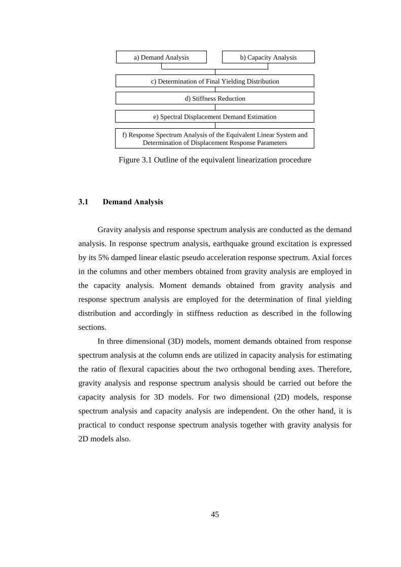
45
Figure 3.1 Outline of the equivalent linearization procedure
3.1 Demand Analysis
Gravity analysis and response spectrum analysis are conducted as the demand
analysis. In response spectrum analysis, earthquake ground excitation is expressed
by its 5% damped linear elastic pseudo acceleration response spectrum. Axial forces
in the columns and other members obtained from gravity analysis are employed in
the capacity analysis. Moment demands obtained from gravity analysis and
response spectrum analysis are employed for the determination of final yielding
distribution and accordingly in stiffness reduction as described in the following
sections.
In three dimensional (3D) models, moment demands obtained from response
spectrum analysis at the column ends are utilized in capacity analysis for estimating
the ratio of flexural capacities about the two orthogonal bending axes. Therefore,
gravity analysis and response spectrum analysis should be carried out before the
capacity analysis for 3D models. For two dimensional (2D) models, response
spectrum analysis and capacity analysis are independent. On the other hand, it is
practical to conduct response spectrum analysis together with gravity analysis for
2D models also.
d) Stiffness Reduction
a) Demand Analysis b) Capacity Analysis
e) Spectral Displacement Demand Estimation
f) Response Spectrum Analysis of the Equivalent Linear System and Determination of Displacement Response Parameters
c) Determination of Final Yielding Distribution
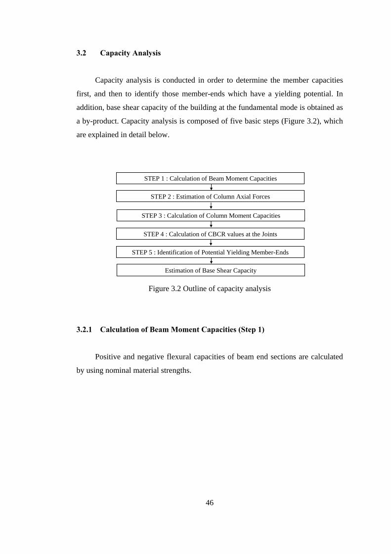
46
3.2 Capacity Analysis
Capacity analysis is conducted in order to determine the member capacities
first, and then to identify those member-ends which have a yielding potential. In
addition, base shear capacity of the building at the fundamental mode is obtained as
a by-product. Capacity analysis is composed of five basic steps (Figure 3.2), which
are explained in detail below.
Figure 3.2 Outline of capacity analysis
3.2.1 Calculation of Beam Moment Capacities (Step 1)
Positive and negative flexural capacities of beam end sections are calculated
by using nominal material strengths.
STEP 1 : Calculation of Beam Moment Capacities
STEP 2 : Estimation of Column Axial Forces
STEP 4 : Calculation of CBCR values at the Joints
STEP 5 : Identification of Potential Yielding Member-Ends
STEP 3 : Calculation of Column Moment Capacities
Estimation of Base Shear Capacity
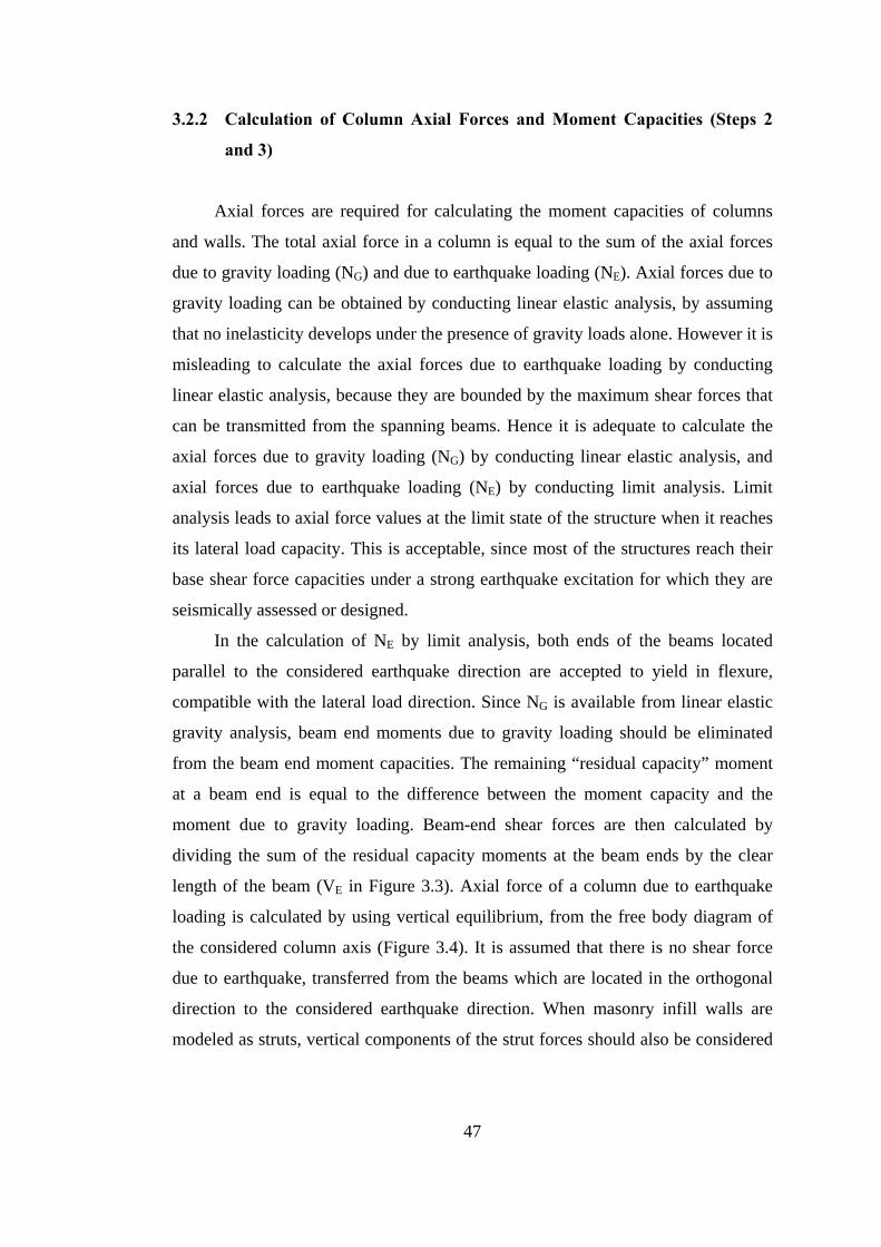
47
3.2.2 Calculation of Column Axial Forces and Moment Capacities (Steps 2
and 3)
Axial forces are required for calculating the moment capacities of columns
and walls. The total axial force in a column is equal to the sum of the axial forces
due to gravity loading (NG) and due to earthquake loading (NE). Axial forces due to
gravity loading can be obtained by conducting linear elastic analysis, by assuming
that no inelasticity develops under the presence of gravity loads alone. However it is
misleading to calculate the axial forces due to earthquake loading by conducting
linear elastic analysis, because they are bounded by the maximum shear forces that
can be transmitted from the spanning beams. Hence it is adequate to calculate the
axial forces due to gravity loading (NG) by conducting linear elastic analysis, and
axial forces due to earthquake loading (NE) by conducting limit analysis. Limit
analysis leads to axial force values at the limit state of the structure when it reaches
its lateral load capacity. This is acceptable, since most of the structures reach their
base shear force capacities under a strong earthquake excitation for which they are
seismically assessed or designed.
In the calculation of NE by limit analysis, both ends of the beams located
parallel to the considered earthquake direction are accepted to yield in flexure,
compatible with the lateral load direction. Since NG is available from linear elastic
gravity analysis, beam end moments due to gravity loading should be eliminated
from the beam end moment capacities. The remaining “residual capacity” moment
at a beam end is equal to the difference between the moment capacity and the
moment due to gravity loading. Beam-end shear forces are then calculated by
dividing the sum of the residual capacity moments at the beam ends by the clear
length of the beam (VE in Figure 3.3). Axial force of a column due to earthquake
loading is calculated by using vertical equilibrium, from the free body diagram of
the considered column axis (Figure 3.4). It is assumed that there is no shear force
due to earthquake, transferred from the beams which are located in the orthogonal
direction to the considered earthquake direction. When masonry infill walls are
modeled as struts, vertical components of the strut forces should also be considered
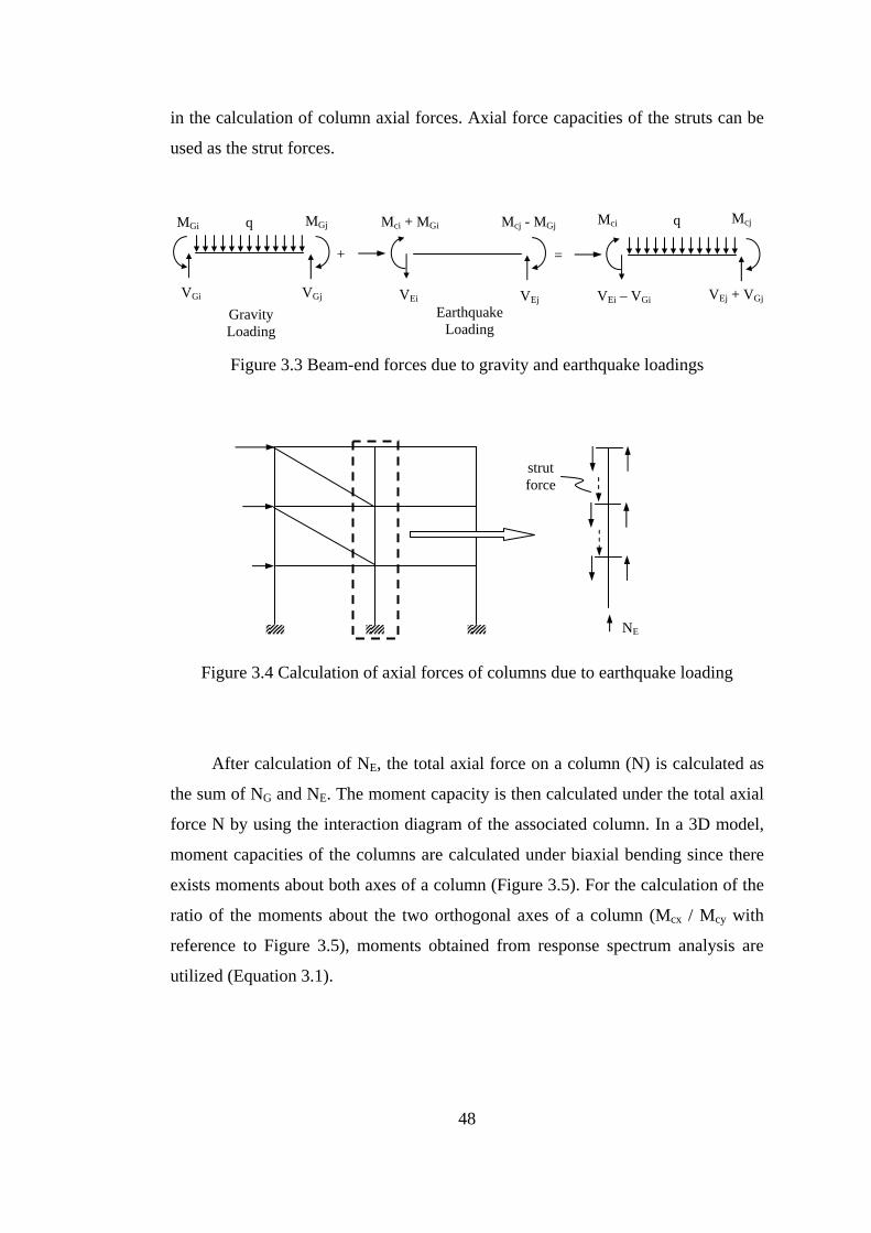
48
in the calculation of column axial forces. Axial force capacities of the struts can be
used as the strut forces.
Figure 3.3 Beam-end forces due to gravity and earthquake loadings
Figure 3.4 Calculation of axial forces of columns due to earthquake loading
After calculation of NE, the total axial force on a column (N) is calculated as
the sum of NG and NE. The moment capacity is then calculated under the total axial
force N by using the interaction diagram of the associated column. In a 3D model,
moment capacities of the columns are calculated under biaxial bending since there
exists moments about both axes of a column (Figure 3.5). For the calculation of the
ratio of the moments about the two orthogonal axes of a column (Mcx / Mcy with
reference to Figure 3.5), moments obtained from response spectrum analysis are
utilized (Equation 3.1).
q
+
MGj Mci + MGi Mci q
Gravity Loading
Earthquake Loading
MGi
VGi VGj VEi VEj
Mcj - MGj
=
Mcj
VEi – VGi VEj + VGj
NE
strut force
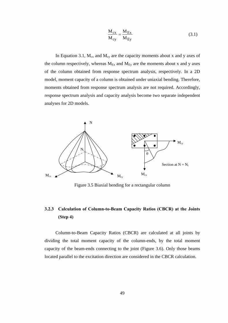
49
Ey
Ex
cy
cxMM
MM
= (3.1)
In Equation 3.1, Mcx and Mcy are the capacity moments about x and y axes of
the column respectively, whereas MEx and MEy are the moments about x and y axes
of the column obtained from response spectrum analysis, respectively. In a 2D
model, moment capacity of a column is obtained under uniaxial bending. Therefore,
moments obtained from response spectrum analysis are not required. Accordingly,
response spectrum analysis and capacity analysis become two separate independent
analyses for 2D models.
Figure 3.5 Biaxial bending for a rectangular column
3.2.3 Calculation of Column-to-Beam Capacity Ratios (CBCR) at the Joints
(Step 4)
Column-to-Beam Capacity Ratios (CBCR) are calculated at all joints by
dividing the total moment capacity of the column-ends, by the total moment
capacity of the beam-ends connecting to the joint (Figure 3.6). Only those beams
located parallel to the excitation direction are considered in the CBCR calculation.
N
Mcx Mcy
Ni
Section at N = Ni
Mcx
Mcy
θ
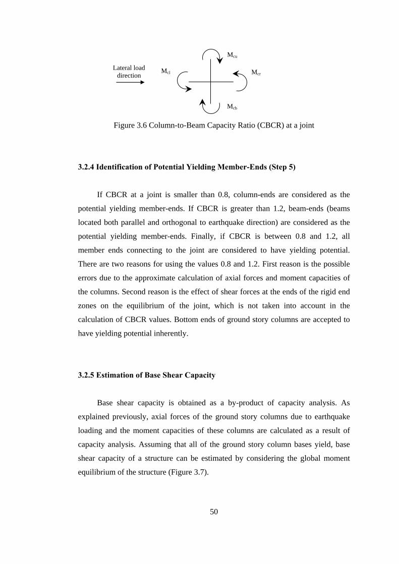
50
Figure 3.6 Column-to-Beam Capacity Ratio (CBCR) at a joint
3.2.4 Identification of Potential Yielding Member-Ends (Step 5)
If CBCR at a joint is smaller than 0.8, column-ends are considered as the
potential yielding member-ends. If CBCR is greater than 1.2, beam-ends (beams
located both parallel and orthogonal to earthquake direction) are considered as the
potential yielding member-ends. Finally, if CBCR is between 0.8 and 1.2, all
member ends connecting to the joint are considered to have yielding potential.
There are two reasons for using the values 0.8 and 1.2. First reason is the possible
errors due to the approximate calculation of axial forces and moment capacities of
the columns. Second reason is the effect of shear forces at the ends of the rigid end
zones on the equilibrium of the joint, which is not taken into account in the
calculation of CBCR values. Bottom ends of ground story columns are accepted to
have yielding potential inherently.
3.2.5 Estimation of Base Shear Capacity
Base shear capacity is obtained as a by-product of capacity analysis. As
explained previously, axial forces of the ground story columns due to earthquake
loading and the moment capacities of these columns are calculated as a result of
capacity analysis. Assuming that all of the ground story column bases yield, base
shear capacity of a structure can be estimated by considering the global moment
equilibrium of the structure (Figure 3.7).
Mcr
Mcb
Mcu
Lateral load direction
Mcl
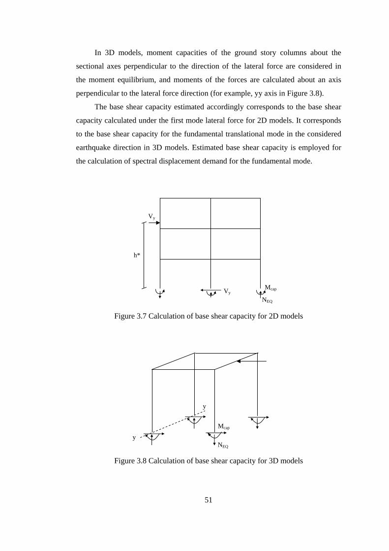
51
In 3D models, moment capacities of the ground story columns about the
sectional axes perpendicular to the direction of the lateral force are considered in
the moment equilibrium, and moments of the forces are calculated about an axis
perpendicular to the lateral force direction (for example, yy axis in Figure 3.8).
The base shear capacity estimated accordingly corresponds to the base shear
capacity calculated under the first mode lateral force for 2D models. It corresponds
to the base shear capacity for the fundamental translational mode in the considered
earthquake direction in 3D models. Estimated base shear capacity is employed for
the calculation of spectral displacement demand for the fundamental mode.
Figure 3.7 Calculation of base shear capacity for 2D models
Figure 3.8 Calculation of base shear capacity for 3D models
y
y
Mcap
NEQ
Vy
h*
Mcap
NEQ Vy
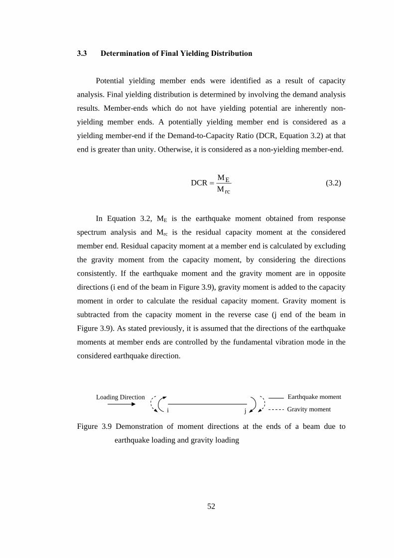
52
3.3 Determination of Final Yielding Distribution
Potential yielding member ends were identified as a result of capacity
analysis. Final yielding distribution is determined by involving the demand analysis
results. Member-ends which do not have yielding potential are inherently non-
yielding member ends. A potentially yielding member end is considered as a
yielding member-end if the Demand-to-Capacity Ratio (DCR, Equation 3.2) at that
end is greater than unity. Otherwise, it is considered as a non-yielding member-end.
rc
EMMDCR = (3.2)
In Equation 3.2, ME is the earthquake moment obtained from response
spectrum analysis and Mrc is the residual capacity moment at the considered
member end. Residual capacity moment at a member end is calculated by excluding
the gravity moment from the capacity moment, by considering the directions
consistently. If the earthquake moment and the gravity moment are in opposite
directions (i end of the beam in Figure 3.9), gravity moment is added to the capacity
moment in order to calculate the residual capacity moment. Gravity moment is
subtracted from the capacity moment in the reverse case (j end of the beam in
Figure 3.9). As stated previously, it is assumed that the directions of the earthquake
moments at member ends are controlled by the fundamental vibration mode in the
considered earthquake direction.
Figure 3.9 Demonstration of moment directions at the ends of a beam due to
earthquake loading and gravity loading
Loading Direction
i j
Earthquake moment
Gravity moment
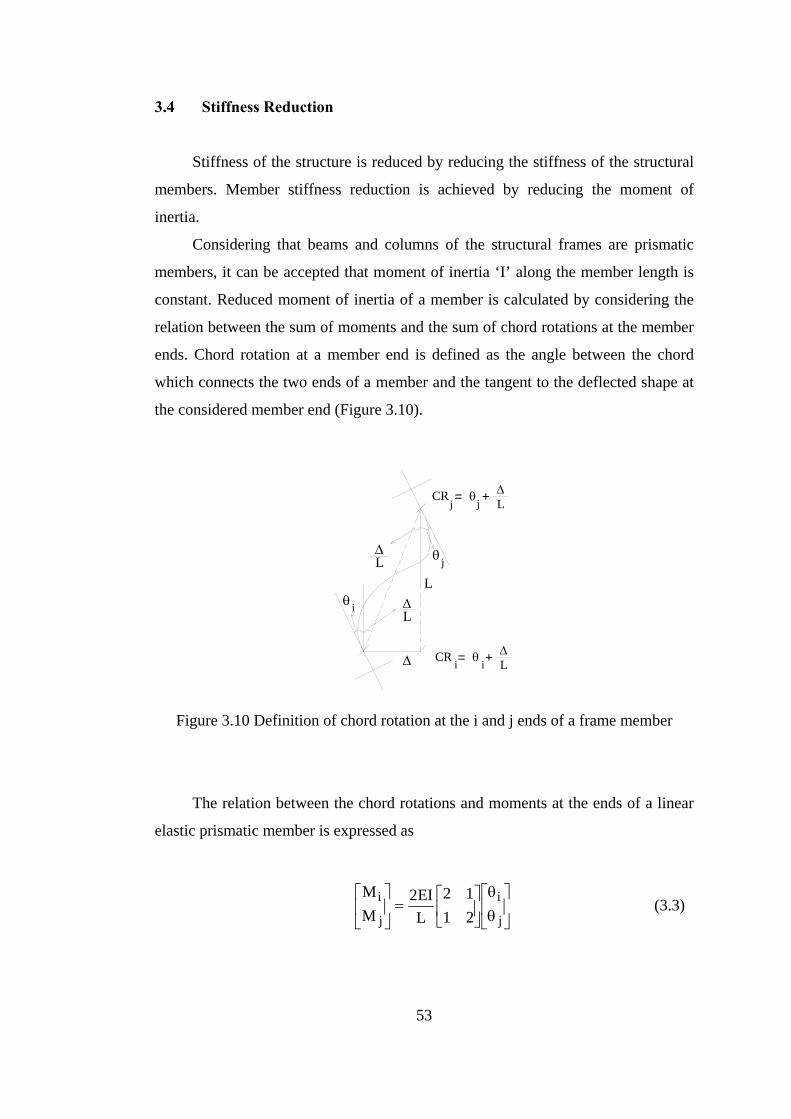
53
3.4 Stiffness Reduction
Stiffness of the structure is reduced by reducing the stiffness of the structural
members. Member stiffness reduction is achieved by reducing the moment of
inertia.
Considering that beams and columns of the structural frames are prismatic
members, it can be accepted that moment of inertia ‘I’ along the member length is
constant. Reduced moment of inertia of a member is calculated by considering the
relation between the sum of moments and the sum of chord rotations at the member
ends. Chord rotation at a member end is defined as the angle between the chord
which connects the two ends of a member and the tangent to the deflected shape at
the considered member end (Figure 3.10).
Figure 3.10 Definition of chord rotation at the i and j ends of a frame member
The relation between the chord rotations and moments at the ends of a linear
elastic prismatic member is expressed as
⎥⎦
⎤⎢⎣
⎡θθ
⎥⎦
⎤⎢⎣
⎡=⎥
⎦
⎤⎢⎣
⎡
j
i
j
i2112
LEI2
MM
(3.3)
θ i ΔL
Δ
L
ΔL θ j
θ iCR
i= + ΔL
CR Δθ +jj = L
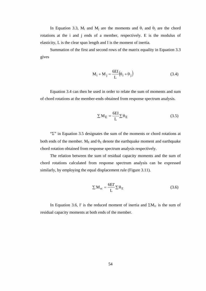
54
In Equation 3.3, Mi and Mj are the moments and θi and θj are the chord
rotations at the i and j ends of a member, respectively. E is the modulus of
elasticity, L is the clear span length and I is the moment of inertia.
Summation of the first and second rows of the matrix equality in Equation 3.3
gives
( )jiji LEI6MM θ+θ=+ (3.4)
Equation 3.4 can then be used in order to relate the sum of moments and sum
of chord rotations at the member-ends obtained from response spectrum analysis.
∑θ=∑ EE LEI6M (3.5)
“Σ” in Equation 3.5 designates the sum of the moments or chord rotations at
both ends of the member. ME and θE denote the earthquake moment and earthquake
chord rotation obtained from response spectrum analysis respectively.
The relation between the sum of residual capacity moments and the sum of
chord rotations calculated from response spectrum analysis can be expressed
similarly, by employing the equal displacement rule (Figure 3.11).
∑θ=∑ Erc L'EI6M (3.6)
In Equation 3.6, I' is the reduced moment of inertia and ΣMrc is the sum of
residual capacity moments at both ends of the member.
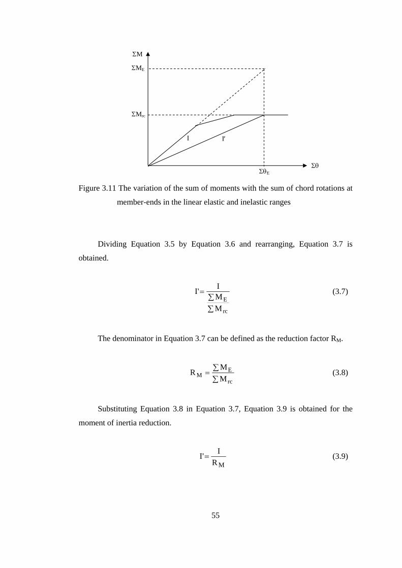
55
Figure 3.11 The variation of the sum of moments with the sum of chord rotations at
member-ends in the linear elastic and inelastic ranges
Dividing Equation 3.5 by Equation 3.6 and rearranging, Equation 3.7 is
obtained.
∑∑
=
rc
EMMI'I (3.7)
The denominator in Equation 3.7 can be defined as the reduction factor RM.
∑∑=
rc
EM M
MR (3.8)
Substituting Equation 3.8 in Equation 3.7, Equation 3.9 is obtained for the
moment of inertia reduction.
MRI'I = (3.9)
I I′
ΣM
Σθ ΣθE
ΣME
ΣMrc
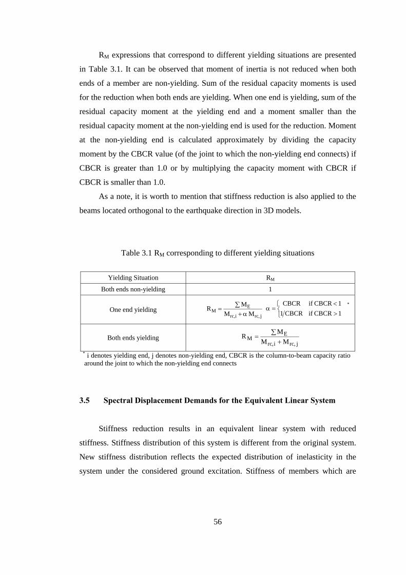
56
RM expressions that correspond to different yielding situations are presented
in Table 3.1. It can be observed that moment of inertia is not reduced when both
ends of a member are non-yielding. Sum of the residual capacity moments is used
for the reduction when both ends are yielding. When one end is yielding, sum of the
residual capacity moment at the yielding end and a moment smaller than the
residual capacity moment at the non-yielding end is used for the reduction. Moment
at the non-yielding end is calculated approximately by dividing the capacity
moment by the CBCR value (of the joint to which the non-yielding end connects) if
CBCR is greater than 1.0 or by multiplying the capacity moment with CBCR if
CBCR is smaller than 1.0.
As a note, it is worth to mention that stiffness reduction is also applied to the
beams located orthogonal to the earthquake direction in 3D models.
Table 3.1 RM corresponding to different yielding situations
Yielding Situation RM
Both ends non-yielding 1
One end yielding
j,rci,rc
EM MM
MRα+
∑= ⎩⎨⎧
><
=α1CBCRifCBCR11CBCRifCBCR *
Both ends yielding j,rci,rc
EM MM
MR
+∑=
* i denotes yielding end, j denotes non-yielding end, CBCR is the column-to-beam capacity ratio around the joint to which the non-yielding end connects
3.5 Spectral Displacement Demands for the Equivalent Linear System
Stiffness reduction results in an equivalent linear system with reduced
stiffness. Stiffness distribution of this system is different from the original system.
New stiffness distribution reflects the expected distribution of inelasticity in the
system under the considered ground excitation. Stiffness of members which are
57
subjected to larger inelastic action are reduced more. On the other hand, stiffness of
those members which are anticipated to behave elastic according to capacity
analysis or demand-to-capacity ratios are not reduced. Therefore, stiffness reduction
determines the relative displacement distribution within the structure. In order to
calculate the actual deformations, global displacement demands should be
determined in addition to the relative displacement distribution.
The global displacement demand of the reduced equivalent linear system can
not be determined by conducting linear response history or response spectrum
analysis under a ground motion unless an increased (equivalent) damping is
imposed for reflecting the hysteretic energy dissipation of the actual system.
Although there are established methods for estimating increased damping in an
equivalent linear SDOF system (Gülkan and Sözen, 1974; Iwan, 1980; Kowalsky,
1994), these methods are more suitable for design purposes since they require the
prior knowledge of ductility ratios (μ) as stated in Chapter 1. In addition, it was
previously stated that equivalent linearization procedures should be employed with
care for the estimation of maximum inelastic displacement demands for systems
with known lateral strength (Akkar and Miranda, 2005). Therefore increased
damping is not employed in this study. Global displacement demands are directly
obtained from the spectral displacement demands in each mode of the equivalent
linear system. These spectral displacement demands are called the target spectral
displacements Sdn*.
Two alternative methods are utilized for the calculation of target spectral
displacements, explained below.
3.5.1 Nonlinear Response History Analysis of the Equivalent SDOF System
Target spectral displacement in the first mode (or the fundamental mode in
the considered earthquake direction in a 3D model) is calculated via nonlinear
response history analysis (NRHA) of the equivalent SDOF system representing this
mode (Sdni*).
58
When the hysteresis behavior of the SDOF system is elastoplastic, three
parameters are required in each mode for conducting nonlinear response history
analysis. These parameters are the period (Tn), the base shear capacity coefficient
(ηny), which is the ratio of base shear capacity to effective modal weight, and the
damping ratio (5% damping ratio is assumed). Tn is obtained from the eigenvalue
analysis of the original structure whereas the base shear capacity in the first mode is
estimated as a result of capacity analysis.
Target spectral displacements of the higher modes are assumed to be equal to
the elastic spectral displacements corresponding to the periods of the original
structure (Sdne*). In fact, the base shear capacity coefficients of the higher modes
are much higher when compared with the first mode base shear capacity coefficient
in structures that do not possess significant irregularity, since the modal masses of
the higher modes are small. Spectral displacements corresponding to the higher
modes usually remain in the elastic range under most ground excitations.
This alternative is referred to as EQL-NL in the following chapters.
3.5.2 Equal Displacement Assumption
In the second alternative, target spectral displacements of all modes are
calculated as the elastic spectral displacements corresponding to the modal vibration
periods of the original (unreduced-stiffness) structure according to the equal
displacement rule (Veletsos and Newmark, 1960). Equal displacement assumption
is valid for the average of many ground motions in the medium and long period
ranges (Miranda, 2000; Miranda, 2001). Therefore it may result in misleading
values for short periods and for individual ground motions. However, target spectral
displacement determination using the equal displacement assumption is employed
as an alternative in this study, because the implementation of equal displacement
rule is much practical with respect to the NRHA of inelastic SDOF systems. The
trade-off between the increase in errors due to equal displacement assumption and
the simplicity of its application is investigated in the case studies.
59
This alternative is referred to as EQL-ED in the following chapters.
3.6 Response Spectrum Analysis of the Equivalent Linear System
Response spectrum analysis of the equivalent linear system is conducted after
the determination of the target spectral displacements. In the application of response
spectrum analysis, modal force vector at any mode ( 'nf ) should be determined such
that the nth mode SDOF system is subjected to a maximum displacement that is
equal to the target spectral displacement calculated for that mode. For this purpose,
pseudo acceleration (PSan*) corresponding to the nth mode target spectral
displacement (Sdn*) at the nth mode period of the equivalent linear system ( '
nT ) is
calculated from Equation 3.10 as explained in Figure 3.12.
2
'n
*n
*n
T2SdPSa ⎟
⎟⎠
⎞⎜⎜⎝
⎛ π= (3.10)
The nth modal force vector ( 'nf ) is calculated from Equation 3.11.
*n
'n
'n
'n PSamφf Γ= (3.11)
In Equation 3.11, 'nφ and '
nΓ are the nth modal vector and nth modal
participation factor for the equivalent linear system, respectively and m is the mass
matrix.
Maximum responses in each mode are calculated by applying the modal force
vector in Equation 3.11 to the equivalent linear structure. Then, the modal responses
are combined by using statistical combination rules. SRSS (square root of sum of
squares, Rosenblueth, 1951) and CQC (complete quadratic combination, Der
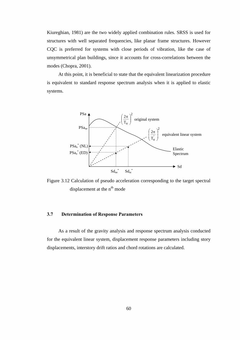
60
Kiureghian, 1981) are the two widely applied combination rules. SRSS is used for
structures with well separated frequencies, like planar frame structures. However
CQC is preferred for systems with close periods of vibration, like the case of
unsymmetrical plan buildings, since it accounts for cross-correlations between the
modes (Chopra, 2001).
At this point, it is beneficial to state that the equivalent linearization procedure
is equivalent to standard response spectrum analysis when it is applied to elastic
systems.
Figure 3.12 Calculation of pseudo acceleration corresponding to the target spectral
displacement at the nth mode
3.7 Determination of Response Parameters
As a result of the gravity analysis and response spectrum analysis conducted
for the equivalent linear system, displacement response parameters including story
displacements, interstory drift ratios and chord rotations are calculated.
PSan* (NL)
Sd
PSa
Elastic Spectrum
Sdni*
PSane
PSan* (ED)
2
'nT
2⎟⎟⎠
⎞⎜⎜⎝
⎛ π
2
nT2
⎟⎟⎠
⎞⎜⎜⎝
⎛ π
Sdne*
original system
equivalent linear system
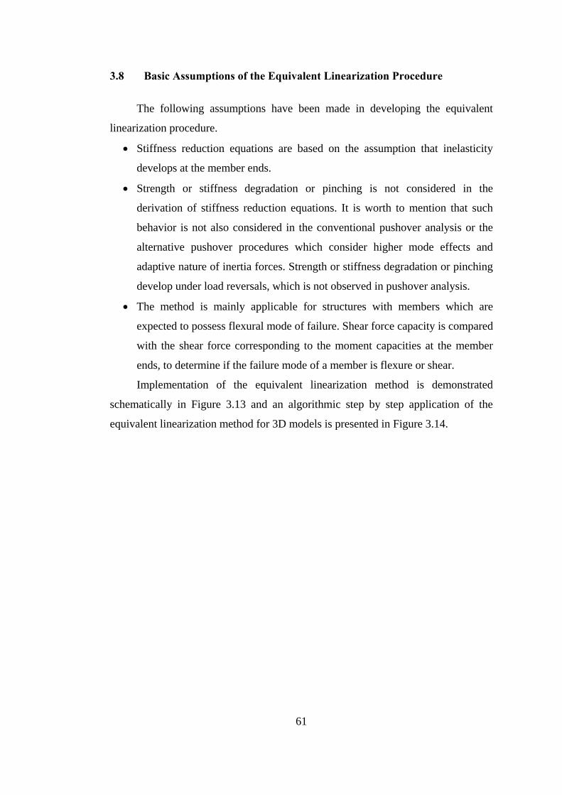
61
3.8 Basic Assumptions of the Equivalent Linearization Procedure
The following assumptions have been made in developing the equivalent
linearization procedure.
• Stiffness reduction equations are based on the assumption that inelasticity
develops at the member ends.
• Strength or stiffness degradation or pinching is not considered in the
derivation of stiffness reduction equations. It is worth to mention that such
behavior is not also considered in the conventional pushover analysis or the
alternative pushover procedures which consider higher mode effects and
adaptive nature of inertia forces. Strength or stiffness degradation or pinching
develop under load reversals, which is not observed in pushover analysis.
• The method is mainly applicable for structures with members which are
expected to possess flexural mode of failure. Shear force capacity is compared
with the shear force corresponding to the moment capacities at the member
ends, to determine if the failure mode of a member is flexure or shear.
Implementation of the equivalent linearization method is demonstrated
schematically in Figure 3.13 and an algorithmic step by step application of the
equivalent linearization method for 3D models is presented in Figure 3.14.
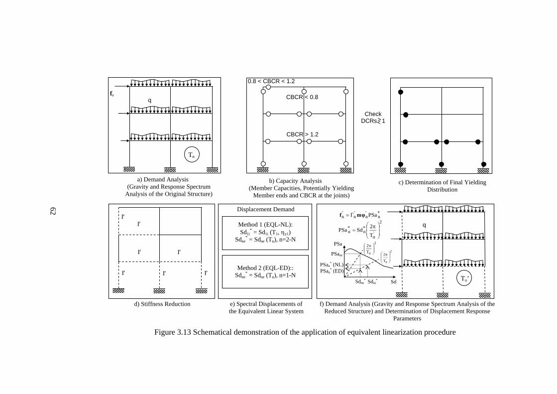
44
Figure 3.13 Schematical demonstration of the application of equivalent linearization procedure
fn
a) Demand Analysis (Gravity and Response Spectrum
Analysis of the Original Structure)
b) Capacity Analysis (Member Capacities, Potentially Yielding
Member ends and CBCR at the joints)
c) Determination of Final Yielding Distribution
Check DCRs 1
d) Stiffness Reduction
I′ I′ I′
I′ I′
I′ I′
Method 1 (EQL-NL): Sd1i
* = Sd1i (T1, ηy1) Sdne
* = Sdne (Tn), n=2-N
Method 2 (EQL-ED)::
Sdne* = Sdne (Tn), n=1-N
e) Spectral Displacements of the Equivalent Linear System
f) Demand Analysis (Gravity and Response Spectrum Analysis of the Reduced Structure) and Determination of Displacement Response
Parameters
CBCR < 0.8
0.8 < CBCR < 1.2
CBCR > 1.2
2
'n
*n
*n
T2SdPSa ⎟
⎟⎠
⎞⎜⎜⎝
⎛ π=
*n
'n
'n
'n PSamφf Γ=
PSan* (NL)
Sd
PSa
Sdni*
PSane
PSan* (ED)
2
'nT
2⎟⎟⎠
⎞⎜⎜⎝
⎛ π
2
nT2
⎟⎟⎠
⎞⎜⎜⎝
⎛ π
Sdne*
<
q
Tn
Displacement Demand
q
Tn’
>
62
63
Combination of the responses (story displacements, interstory drift ratios, chord rotations) from the application of the modal force in each mode by a suitable combination rule (eg. SRSS or CQC) and superposition of these
responses with those of gravity analysis
Figure 3.14 Flowchart of the equivalent linearization procedure for a 3D model with reference to Figure 3.13
Determination of Final Yielding Distribution
3D Analysis Model For Linear Elastic Analysis
Gravity Analysis and Response Spectrum Analysis
Calculation of Moment Capacities at Beam Ends
Determination of Residual Moments at the Ends of Beams Located Parallel to the Considered Earthquake Direction
Determination of Shear Forces at the Ends of Beams Located Parallel to the Considered Earthquake Direction
Estimation of Column Axial Forces using the Transferred Shear Forces
Calculation of CBCR Values at the Joints
Identification of Potential Yielding Member Ends
Determination of Base Shear Capacity Coefficient Corresponding to the Fundamental Mode in the Considered Earthquake Direction (ηy1)
Reduction of Stiffness
If at least one of the ends of a member is yielding
DCR at a Potential Yielding Member End >? 1
Determination of Spectral Displacement Demands For the Equivalent Linear System
Method 1 (EQL-NL): Sd1i
* = Sd1i (T1, η1y) Sdne
* = Sdne (Tn), n=2-N
Method 2 (EQL-ED): Sdne
* = Sdne (Tn), n=1-N
a)
b)
c) Yes
Yielding Member End
No
Nonyielding Member End
MRI'I =
d)
e)
Calculation of Moment Capacities of Columns
Response spectrum Analysis of the Equivalent Linear System
Modal force at mode n Pseudo acceleration at mode n
f)
2
'n
*n
*n
T
2SdPSa⎟⎟
⎠
⎞
⎜⎜
⎝
⎛ π= *
n'n
'n
'n PSamφf Γ=
64
CHAPTER 4
GROUND MOTIONS EMPLOYED IN CASE STUDIES
Ground motions which contain pulses especially in their velocity and
displacement traces impose larger demands on structures than ordinary ground
motions. These ground motions are usually near-fault ground motions with forward
directivity effects (Alavi and Krawinkler, 2001; 2004). Therefore, ground motions
utilized in this study are divided into two sets, designated as pulse type ground
motion set (96 ground motions) and ordinary ground motion set (66 ground
motions). Pulse type ground motion set consists of ground motions possessing
significant velocity pulses with PGV greater than 35 cm/s. Ordinary ground motion
set consists of ground motions which do not satisfy the above criterion. A grouping
based on the existence of pulse signals was previously employed by Akkar et al.
(2005).
All of the utilized ground motions are downloaded from PEER strong motion
database. Important features of these ground motions are listed in Tables 4.1 and
4.2.
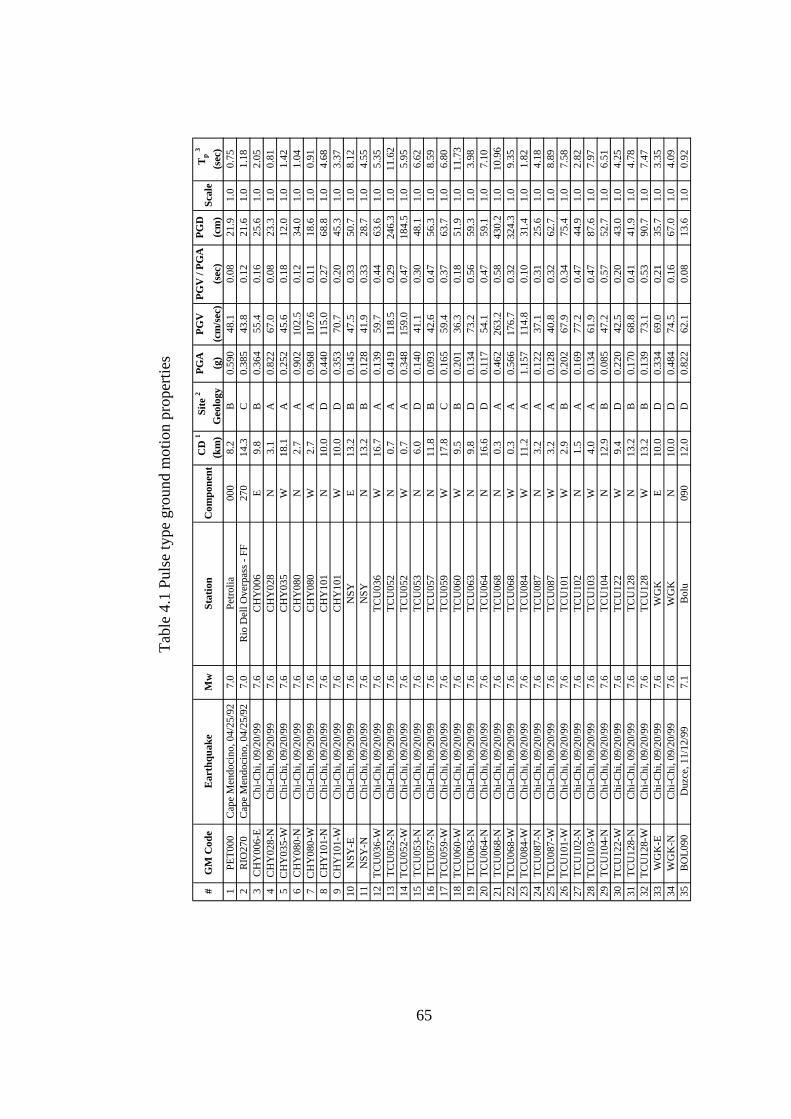
65
Tabl
e 4.
1 Pu
lse
type
gro
und
mot
ion
prop
ertie
s
#G
M C
ode
Ear
thqu
ake
Mw
Stat
ion
Com
pone
nt C
D 1
(km
) S
ite 2
Geo
logy
PGA
(g
)PG
V
(cm
/sec
)PG
V /
PGA
(s
ec)
PGD
(c
m)
Scal
e T
p 3
(sec
)1
PET0
00C
ape
Men
doci
no, 0
4/25
/92
7.0
Petro
lia00
08.
2B
0.59
048
.10.
0821
.91.
00.
752
RIO
270
Cap
e M
endo
cino
, 04/
25/9
27.
0R
io D
ell O
verp
ass -
FF
270
14.3
C0.
385
43.8
0.12
21.6
1.0
1.18
3C
HY
006-
EC
hi-C
hi, 0
9/20
/99
7.6
CH
Y00
6E
9.8
B0.
364
55.4
0.16
25.6
1.0
2.05
4C
HY
028-
NC
hi-C
hi, 0
9/20
/99
7.6
CH
Y02
8N
3.1
A0.
822
67.0
0.08
23.3
1.0
0.81
5C
HY
035-
WC
hi-C
hi, 0
9/20
/99
7.6
CH
Y03
5W
18.1
A0.
252
45.6
0.18
12.0
1.0
1.42
6C
HY
080-
NC
hi-C
hi, 0
9/20
/99
7.6
CH
Y08
0N
2.7
A0.
902
102.
50.
1234
.01.
01.
047
CH
Y08
0-W
Chi
-Chi
, 09/
20/9
97.
6C
HY
080
W2.
7A
0.96
810
7.6
0.11
18.6
1.0
0.91
8C
HY
101-
NC
hi-C
hi, 0
9/20
/99
7.6
CH
Y10
1N
10.0
D0.
440
115.
00.
2768
.81.
04.
689
CH
Y10
1-W
Chi
-Chi
, 09/
20/9
97.
6C
HY
101
W10
.0D
0.35
370
.70.
2045
.31.
03.
3710
NSY
-EC
hi-C
hi, 0
9/20
/99
7.6
NSY
E13
.2B
0.14
547
.50.
3350
.71.
08.
1211
NSY
-NC
hi-C
hi, 0
9/20
/99
7.6
NSY
N13
.2B
0.12
841
.90.
3328
.71.
04.
5512
TCU
036-
WC
hi-C
hi, 0
9/20
/99
7.6
TCU
036
W16
.7A
0.13
959
.70.
4463
.61.
05.
3513
TCU
052-
NC
hi-C
hi, 0
9/20
/99
7.6
TCU
052
N0.
7A
0.41
911
8.5
0.29
246.
31.
011
.62
14TC
U05
2-W
Chi
-Chi
, 09/
20/9
97.
6TC
U05
2W
0.7
A0.
348
159.
00.
4718
4.5
1.0
5.95
15TC
U05
3-N
Chi
-Chi
, 09/
20/9
97.
6TC
U05
3N
6.0
D0.
140
41.1
0.30
48.1
1.0
6.62
16TC
U05
7-N
Chi
-Chi
, 09/
20/9
97.
6TC
U05
7N
11.8
B0.
093
42.6
0.47
56.3
1.0
8.59
17TC
U05
9-W
Chi
-Chi
, 09/
20/9
97.
6TC
U05
9W
17.8
C0.
165
59.4
0.37
63.7
1.0
6.80
18TC
U06
0-W
Chi
-Chi
, 09/
20/9
97.
6TC
U06
0W
9.5
B0.
201
36.3
0.18
51.9
1.0
11.7
319
TCU
063-
NC
hi-C
hi, 0
9/20
/99
7.6
TCU
063
N9.
8D
0.13
473
.20.
5659
.31.
03.
9820
TCU
064-
NC
hi-C
hi, 0
9/20
/99
7.6
TCU
064
N16
.6D
0.11
754
.10.
4759
.11.
07.
1021
TCU
068-
NC
hi-C
hi, 0
9/20
/99
7.6
TCU
068
N0.
3A
0.46
226
3.2
0.58
430.
21.
010
.96
22TC
U06
8-W
Chi
-Chi
, 09/
20/9
97.
6TC
U06
8W
0.3
A0.
566
176.
70.
3232
4.3
1.0
9.35
23TC
U08
4-W
Chi
-Chi
, 09/
20/9
97.
6TC
U08
4W
11.2
A1.
157
114.
80.
1031
.41.
01.
8224
TCU
087-
NC
hi-C
hi, 0
9/20
/99
7.6
TCU
087
N3.
2A
0.12
237
.10.
3125
.61.
04.
1825
TCU
087-
WC
hi-C
hi, 0
9/20
/99
7.6
TCU
087
W3.
2A
0.12
840
.80.
3262
.71.
08.
8926
TCU
101-
WC
hi-C
hi, 0
9/20
/99
7.6
TCU
101
W2.
9B
0.20
267
.90.
3475
.41.
07.
5827
TCU
102-
NC
hi-C
hi, 0
9/20
/99
7.6
TCU
102
N1.
5A
0.16
977
.20.
4744
.91.
02.
8228
TCU
103-
WC
hi-C
hi, 0
9/20
/99
7.6
TCU
103
W4.
0A
0.13
461
.90.
4787
.61.
07.
9729
TCU
104-
NC
hi-C
hi, 0
9/20
/99
7.6
TCU
104
N12
.9B
0.08
547
.20.
5752
.71.
06.
5130
TCU
122-
WC
hi-C
hi, 0
9/20
/99
7.6
TCU
122
W9.
4D
0.22
042
.50.
2043
.01.
04.
2531
TCU
128-
NC
hi-C
hi, 0
9/20
/99
7.6
TCU
128
N13
.2B
0.17
068
.80.
4141
.91.
04.
7832
TCU
128-
WC
hi-C
hi, 0
9/20
/99
7.6
TCU
128
W13
.2B
0.13
973
.10.
5390
.71.
07.
4733
WG
K-E
Chi
-Chi
, 09/
20/9
97.
6W
GK
E10
.0D
0.33
469
.00.
2135
.71.
03.
3534
WG
K-N
Chi
-Chi
, 09/
20/9
97.
6W
GK
N10
.0D
0.48
474
.50.
1667
.01.
04.
0935
BO
L090
Duz
ce, 1
1/12
/99
7.1
Bolu
090
12.0
D0.
822
62.1
0.08
13.6
1.0
0.92
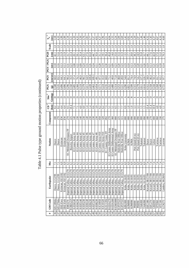
66
Tabl
e 4.
1 Pu
lse
type
gro
und
mot
ion
prop
ertie
s (co
ntin
ued)
#G
M C
ode
Ear
thqu
ake
Mw
Stat
ion
Com
pone
nt C
D 1
(km
) S
ite 2
Geo
logy
PGA
(g
)PG
V
(cm
/sec
)PG
V /
PGA
(s
ec)
PGD
(c
m)
Scal
e T
p 3
(sec
)36
DZC
180d
zcD
uzce
, 11/
12/9
97.
1D
uzce
180
8.2
D0.
348
60.0
0.18
42.1
1.0
5.58
37D
ZC27
0dzc
Duz
ce, 1
1/12
/99
7.1
Duz
ce27
08.
2D
0.53
583
.50.
1651
.61.
04.
1038
ERZ-
Ewa
Erzi
ncan
, 03/
13/9
26.
9Er
zinc
anEW
4.4
D0.
496
64.3
0.13
21.9
1.5
1.99
39ER
Z-Ew
bEr
zinc
an, 0
3/13
/92
6.9
Erzi
ncan
EW4.
4D
0.49
664
.30.
1321
.91.
01.
9940
EMO
270
Impe
rial V
alle
y, 1
0/15
/79
6.5
EC M
elol
and
Ove
rpas
s FF
270
0.5
D0.
296
90.4
0.31
31.7
1.0
3.18
41H
-BR
A22
5Im
peria
l Val
ley,
10/
15/7
96.
5Br
awle
y A
irpor
t22
510
.4D
0.16
035
.90.
2322
.41.
03.
2142
H-E
0414
0Im
peria
l Val
ley,
10/
15/7
96.
5El
Cen
tro A
rray
#4
140
7.1
D0.
485
37.4
0.08
20.1
1.0
1.20
43H
-E04
230
Impe
rial V
alle
y, 1
0/15
/79
6.5
El C
entro
Arr
ay #
423
07.
1D
0.36
076
.50.
2259
.11.
04.
3544
H-E
0514
0Im
peria
l Val
ley,
10/
15/7
96.
5El
Cen
tro A
rray
#5
140
4.0
D0.
519
46.9
0.09
35.4
1.0
3.39
45H
-E05
230
Impe
rial V
alle
y, 1
0/15
/79
6.5
El C
entro
Arr
ay #
523
04.
0D
0.37
990
.50.
2463
.11.
03.
7646
H-E
0614
0Im
peria
l Val
ley,
10/
15/7
96.
5El
Cen
tro A
rray
#6
140
1.4
D0.
411
64.9
0.16
27.6
1.0
2.83
47H
-E06
230
Impe
rial V
alle
y, 1
0/15
/79
6.5
El C
entro
Arr
ay #
623
01.
4D
0.43
910
9.8
0.26
65.8
1.0
3.77
48H
-E07
230
Impe
rial V
alle
y, 1
0/15
/79
6.5
El C
entro
Arr
ay #
723
00.
6D
0.46
310
9.3
0.24
44.7
1.0
3.37
49H
-E08
230
Impe
rial V
alle
y, 1
0/15
/79
6.5
El C
entro
Arr
ay #
823
03.
9D
0.45
449
.10.
1135
.61.
04.
0250
H-E
1005
0Im
peria
l Val
ley,
10/
15/7
96.
5El
Cen
tro A
rray
#10
050
6.2
D0.
171
47.5
0.28
31.1
1.0
4.37
51H
-E10
320
Impe
rial V
alle
y, 1
0/15
/79
6.5
El C
entro
Arr
ay #
1032
06.
2D
0.22
441
.00.
1919
.51.
01.
9652
H-E
CC
092
Impe
rial V
alle
y, 1
0/15
/79
6.5
EC C
ount
y C
ente
r FF
092
7.3
D0.
235
68.8
0.30
39.4
1.0
3.51
53H
-ED
A27
0Im
peria
l Val
ley,
10/
15/7
96.
5El
Cen
tro D
iffer
entia
l Arra
y27
05.
1D
0.35
271
.20.
2145
.81.
04.
0454
H-E
DA
360
Impe
rial V
alle
y, 1
0/15
/79
6.5
El C
entro
Diff
eren
tial A
rray
360
5.1
D0.
480
40.8
0.09
14.0
1.0
1.55
55H
-EM
O00
0Im
peria
l Val
ley,
10/
15/7
96.
5EC
Mel
olan
d O
verp
ass F
F00
00.
5D
0.31
471
.80.
2325
.61.
03.
2456
H-H
VP2
25Im
peria
l Val
ley,
10/
15/7
96.
5H
oltv
ille
Post
Off
ice
225
7.7
D0.
253
48.8
0.20
31.6
1.0
5.09
57H
-HV
P315
Impe
rial V
alle
y, 1
0/15
/79
6.5
Hol
tvill
e Po
st O
ffic
e31
57.
7D
0.22
149
.80.
2331
.91.
03.
6958
KBU
000
Kob
e, 0
1/16
/95
6.9
Kob
e U
nive
rsity
000
0.9
A0.
290
54.8
0.19
13.5
1.0
1.42
59K
JM00
0K
obe,
01/
16/9
56.
9K
JMA
000
1.0
B0.
821
81.3
0.10
17.7
1.0
0.92
60K
JM09
0K
obe,
01/
16/9
56.
9K
JMA
090
1.0
B0.
599
74.4
0.13
20.0
1.0
1.26
61PR
I000
Kob
e, 0
1/16
/95
6.9
Port
Isla
nd (0
m)
000
3.3
E0.
315
74.9
0.24
38.3
1.0
2.29
62PR
I090
Kob
e, 0
1/16
/95
6.9
Port
Isla
nd (0
m)
090
3.3
E0.
278
54.2
0.20
24.9
1.0
1.97
63TA
K00
0K
obe,
01/
16/9
56.
9Ta
kato
ri00
01.
5E
0.61
112
7.2
0.21
35.8
1.0
1.44
64TA
K09
0K
obe,
01/
16/9
56.
9Ta
kato
ri09
01.
5E
0.61
612
0.7
0.20
32.7
1.0
1.46
65D
ZC18
0K
ocae
li, 0
8/17
/99
7.4
Duz
ce18
015
.4D
0.31
258
.90.
1944
.11.
04.
3266
DZC
270
Koc
aeli,
08/
17/9
97.
4D
uzce
270
15.4
D0.
358
46.4
0.13
17.6
1.0
1.45
67G
BZ00
0K
ocae
li, 0
8/17
/99
7.4
Geb
ze00
010
.9A
0.24
450
.30.
2142
.81.
04.
3768
YPT
060
Koc
aeli,
08/
17/9
97.
4Y
arim
ca06
04.
8D
0.26
865
.70.
2557
.01.
04.
6769
YPT
330
Koc
aeli,
08/
17/9
97.
4Y
arim
ca33
04.
8D
0.34
962
.20.
1851
.01.
04.
1670
LCN
275
Land
ers,
06/2
8/92
7.3
Luce
rne
275
1.1
A0.
721
97.7
0.14
70.3
1.0
4.60

67
Tabl
e 4.
1 Pu
lse
type
gro
und
mot
ion
prop
ertie
s (co
ntin
ued)
1 CD
: Clo
sest
dis
tanc
e to
faul
t rup
ture
2 S
ite g
eolo
gy b
ased
on
the
third
lette
r of G
eom
atrix
’s c
lass
ifica
tion
A =
Roc
k. In
stru
men
t on
rock
(Vs >
600
m/s
ec) o
r < 5
m o
f soi
l ove
r roc
k, B
= S
hallo
w (s
tiff)
soil.
Inst
rum
ent o
n/in
soil
prof
ile u
p to
20m
thic
k ov
erly
ing
rock
. C
= D
eep
narr
ow so
il. In
stru
men
t on/
in so
il pr
ofile
at l
east
20m
thic
k ov
erly
ing
rock
, in
a na
rrow
can
yon
or v
alle
y no
mor
e th
an se
vera
l km
wid
e.
D =
Dee
p br
oad
soil.
Inst
rum
ent o
n/in
soil
prof
ile a
t lea
st 2
0m th
ick
over
lyin
g ro
ck, i
n a
broa
d va
lley,
E =
Sof
t dee
p so
il. In
stru
men
t on/
in d
eep
soil
prof
ile w
ith
ave
rage
Vs <
150
m/s
ec.
3 Tp:
Puls
e pe
riod
#G
M C
ode
Ear
thqu
ake
Mw
Stat
ion
Com
pone
nt C
D 1
(km
) S
ite 2
Geo
logy
PGA
(g
)PG
V
(cm
/sec
)PG
V /
PGA
(s
ec)
PGD
(c
m)
Scal
e T
p 3
(sec
)71
CLS
090
Lom
a Pr
ieta
, 10/
18/8
97.
0C
orra
litos
090
3.9
A0.
479
45.2
0.10
11.3
1.0
0.70
72G
0209
0Lo
ma
Prie
ta, 1
0/18
/89
7.0
Gilr
oy A
rray
#2
090
13.7
D0.
322
39.1
0.12
12.1
1.0
1.34
73G
0309
0Lo
ma
Prie
ta, 1
0/18
/89
7.0
Gilr
oy A
rray
#3
090
13.0
D0.
367
44.7
0.12
19.3
1.0
2.08
74LE
X00
0Lo
ma
Prie
ta, 1
0/18
/89
7.0
Los G
atos
- Le
ton
Dam
000
5.0
A0.
420
73.5
0.18
20.0
1.0
1.31
75LE
X09
0Lo
ma
Prie
ta, 1
0/18
/89
7.0
Los G
atos
- Le
ton
Dam
090
5.0
A0.
433
86.3
0.20
30.1
1.0
1.50
76ST
G09
0Lo
ma
Prie
ta, 1
0/18
/89
7.0
Sara
toga
- A
loha
Ave
090
8.5
D0.
324
42.6
0.13
27.6
1.0
3.09
77W
VC
000
Lom
a Pr
ieta
, 10/
18/8
97.
0Sa
rato
ga -
W V
alle
y C
oll.
000
9.3
D0.
255
42.4
0.17
19.5
1.0
1.74
78C
YC
285
Mor
gan
Hill
, 04/
24/8
46.
1C
oyot
e La
ke D
am (S
W A
but)
285
0.5
A1.
298
80.8
0.06
9.6
1.0
0.86
79N
PS21
0N
. Pal
m S
prin
gs, 0
7/08
/86
6.2
Nor
th P
alm
Spr
ings
210
4.0
D0.
594
73.2
0.13
11.5
1.0
1.23
80C
NP1
96N
orth
ridge
, 01/
17/9
46.
7C
anog
a Pa
rk -
Topa
nga
Can
196
14.7
D0.
420
60.7
0.15
20.3
1.0
1.42
81LO
S270
Nor
thrid
ge, 0
1/17
/94
6.7
Can
yon
Cou
ntry
- W
Los
t Can
y27
012
.4C
0.48
244
.90.
0912
.51.
00.
6982
NW
H36
0N
orth
ridge
, 01/
17/9
46.
7N
ewha
ll - F
ire S
ta36
05.
9D
0.59
096
.90.
1738
.11.
01.
3483
RIN
228
Nor
thrid
ge, 0
1/17
/94
6.7
Rin
aldi
Rec
eivi
ng S
ta22
87.
1C
0.83
816
6.0
0.20
28.1
1.0
1.16
84SC
S052
Nor
thrid
ge, 0
1/17
/94
6.7
Sylm
ar -
Con
verte
r Sta
052
5.4
D0.
613
117.
40.
2054
.31.
02.
5085
SCS1
42N
orth
ridge
, 01/
17/9
46.
7Sy
lmar
- C
onve
rter S
ta14
25.
4D
0.89
710
2.2
0.12
45.1
1.0
1.21
86SP
V27
0N
orth
ridge
, 01/
17/9
46.
7Se
pulv
eda
VA
270
8.9
D0.
753
84.5
0.11
18.7
1.0
1.06
87SY
L090
Nor
thrid
ge, 0
1/17
/94
6.7
Sylm
ar -
Oliv
e V
iew
Med
FF
090
5.3
D0.
605
78.1
0.13
16.8
1.0
2.08
88SY
L360
Nor
thrid
ge, 0
1/17
/94
6.7
Sylm
ar -
Oliv
e V
iew
Med
FF
360
5.3
D0.
843
129.
40.
1631
.91.
01.
9489
TAR
090
Nor
thrid
ge, 0
1/17
/94
6.7
Tarz
ana
- Ced
ar H
ill A
090
15.6
B1.
779
109.
60.
0632
.91.
00.
7890
WPI
046
Nor
thrid
ge, 0
1/17
/94
6.7
New
hall
- W P
ico
Can
yon
Rd.
046
5.5
B0.
455
92.8
0.21
56.6
1.0
2.55
91W
PI31
6N
orth
ridge
, 01/
17/9
46.
7N
ewha
ll - W
Pic
o C
anyo
n R
d.31
65.
5B
0.32
567
.40.
2116
.11.
01.
9192
PCD
164
San
Fern
ando
, 02/
09/7
16.
6Pa
coim
a D
am16
42.
8B
1.22
611
2.5
0.09
35.4
1.0
1.32
93PC
D25
4Sa
n Fe
rnan
do, 0
2/09
/71
6.6
Paco
ima
Dam
254
2.8
B1.
160
54.1
0.05
11.8
1.0
0.47
94B
-ICC
090
Supe
rstit
ion
Hill
s, 11
/24/
876.
6El
Cen
tro Im
p. C
o. C
ent
090
18.2
D0.
258
40.9
0.16
20.1
1.0
2.41
95B
-PTS
225
Supe
rstit
ion
Hill
s, 11
/24/
876.
6Pa
rach
ute
Test
Site
225
1.0
D0.
455
112.
00.
2552
.81.
02.
2296
TAB-
LNTa
bas-
Iran,
09/
16/7
87.
5Ta
bas
LN2.
1A
0.83
697
.80.
1238
.71.
01.
54
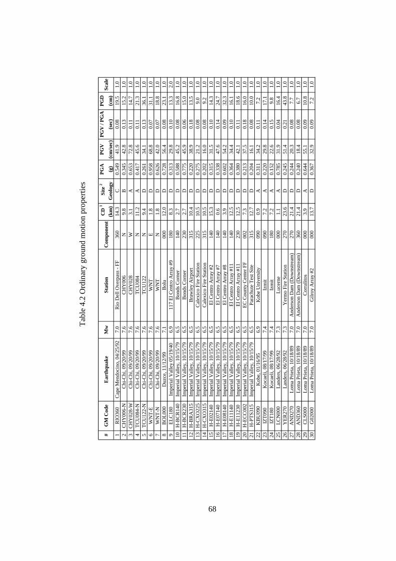
68
Tabl
e 4.
2 O
rdin
ary
grou
nd m
otio
n pr
oper
ties
#G
M C
ode
Ear
thqu
ake
Mw
Stat
ion
Com
pone
nt C
D 1
(km
) S
ite 2
Geo
logy
PGA
(g
)PG
V
(cm
/sec
)PG
V /
PGA
(s
ec)
PGD
(c
m)
Scal
e
1R
IO36
0C
ape
Men
doci
no, 0
4/25
/92
7.0
Rio
Del
l Ove
rpas
s - F
F36
014
.3C
0.54
941
.90.
0819
.51.
02
CH
Y00
6-N
Chi
-Chi
, 09/
20/9
97.
6C
HY
006
N9.
8B
0.34
542
.80.
1315
.21.
03
CH
Y02
8-W
Chi
-Chi
, 09/
20/9
97.
6C
HY
028
W3.
1A
0.65
372
.80.
1114
.71.
04
TCU
084-
NC
hi-C
hi, 0
9/20
/99
7.6
TCU
084
N11
.2A
0.41
745
.60.
1121
.31.
05
TCU
122-
NC
hi-C
hi, 0
9/20
/99
7.6
TCU
122
N9.
4D
0.26
134
.10.
1336
.11.
06
WN
T-E
Chi
-Chi
, 09/
20/9
97.
6W
NT
E1.
8D
0.95
868
.80.
0731
.11.
07
WN
T-N
Chi
-Chi
, 09/
20/9
97.
6W
NT
N1.
8D
0.62
642
.00.
0718
.81.
08
BO
L000
Duz
ce, 1
1/12
/99
7.1
Bol
u00
012
.0D
0.72
856
.40.
0823
.11.
09
ELC
180
Impe
rial V
alle
y 05
/19/
406.
911
7 El
Cen
tro A
rray
#9
180
8.3
D0.
313
29.8
0.10
13.3
2.0
10H
-BC
R14
0Im
peria
l Val
ley,
10/
15/7
96.
5B
onds
Cor
ner
140
2.7
D0.
588
45.2
0.08
16.8
1.0
11H
-BC
R23
0Im
peria
l Val
ley,
10/
15/7
96.
5B
onds
Cor
ner
230
2.7
D0.
775
45.9
0.06
15.0
1.0
12H
-BR
A31
5Im
peria
l Val
ley,
10/
15/7
96.
5B
raw
ley
Airp
ort
315
10.4
D0.
220
38.9
0.18
13.5
1.0
13H
-CX
O22
5Im
peria
l Val
ley,
10/
15/7
96.
5C
alex
ico
Fire
Sta
tion
225
10.5
D0.
275
21.2
0.08
9.0
1.0
14H
-CX
O31
5Im
peria
l Val
ley,
10/
15/7
96.
5C
alex
ico
Fire
Sta
tion
315
10.5
D0.
202
16.0
0.08
9.2
1.0
15H
-E02
140
Impe
rial V
alle
y, 1
0/15
/79
6.5
El C
entro
Arr
ay #
214
015
.3D
0.31
531
.50.
1014
.31.
016
H-E
0714
0Im
peria
l Val
ley,
10/
15/7
96.
5El
Cen
tro A
rray
#7
140
0.6
D0.
338
47.6
0.14
24.7
1.0
17H
-E08
140
Impe
rial V
alle
y, 1
0/15
/79
6.5
El C
entro
Arr
ay #
814
03.
9D
0.60
254
.20.
0932
.31.
018
H-E
1114
0Im
peria
l Val
ley,
10/
15/7
96.
5El
Cen
tro A
rray
#11
140
12.5
D0.
364
34.4
0.10
16.1
1.0
19H
-E11
230
Impe
rial V
alle
y, 1
0/15
/79
6.5
El C
entro
Arr
ay #
1123
012
.5D
0.38
042
.10.
1118
.61.
020
H-E
CC
002
Impe
rial V
alle
y, 1
0/15
/79
6.5
EC C
ount
y C
ente
r FF
002
7.3
D0.
213
37.5
0.18
16.0
1.0
21H
-PTS
315
Impe
rial V
alle
y, 1
0/15
/79
6.5
Para
chut
e Te
st S
ite31
512
.7D
0.20
416
.10.
0810
.01.
022
KB
U09
0K
obe,
01/
16/9
56.
9K
obe
Uni
vers
ity09
00.
9A
0.31
134
.20.
117.
21.
023
IZT0
90K
ocae
li, 0
8/17
/99
7.4
Izm
it09
07.
2A
0.22
029
.80.
1417
.11.
024
IZT1
80K
ocae
li, 0
8/17
/99
7.4
Izm
it18
07.
2A
0.15
222
.60.
159.
81.
025
LCN
000
Land
ers,
06/2
8/92
7.3
Luce
rne
000
1.1
A0.
785
31.9
0.04
16.4
1.0
26Y
ER27
0La
nder
s, 06
/28/
927.
3Y
erm
o Fi
re S
tatio
n27
023
.6D
0.24
551
.40.
2143
.81.
027
AN
D27
0Lo
ma
Prie
ta, 1
0/18
/89
7.0
And
erso
n D
am (D
owns
tream
)27
021
.4D
0.24
420
.30.
087.
71.
028
AN
D36
0Lo
ma
Prie
ta, 1
0/18
/89
7.0
And
erso
n D
am (D
owns
tream
)36
021
.4D
0.24
018
.40.
086.
71.
029
CLS
000
Lom
a Pr
ieta
, 10/
18/8
97.
0C
orra
litos
000
3.9
A0.
644
55.1
0.09
10.8
1.0
30G
0200
0Lo
ma
Prie
ta, 1
0/18
/89
7.0
Gilr
oy A
rray
#2
000
13.7
D0.
367
32.9
0.09
7.2
1.0

69
Tabl
e 4.
2 O
rdin
ary
grou
nd m
otio
n pr
oper
ties (
cont
inue
d)
#G
M C
ode
Ear
thqu
ake
Mw
Stat
ion
Com
pone
nt C
D 1
(km
) S
ite 2
Geo
logy
PGA
(g
)PG
V
(cm
/sec
)PG
V /
PGA
(s
ec)
PGD
(c
m)
Scal
e
31G
0300
0Lo
ma
Prie
ta, 1
0/18
/89
7.0
Gilr
oy A
rray
#3
000
13.0
D0.
555
35.7
0.07
8.3
1.0
32G
0400
0Lo
ma
Prie
ta, 1
0/18
/89
7.0
Gilr
oy A
rray
#4
000
14.3
D0.
417
38.8
0.09
7.1
1.0
33G
0409
0Lo
ma
Prie
ta, 1
0/18
/89
7.0
Gilr
oy A
rray
#4
090
14.3
D0.
212
37.9
0.18
10.1
1.0
34G
GB
270
Lom
a Pr
ieta
, 10/
18/8
97.
0G
olde
n G
ate
Brid
ge27
079
.8A
0.23
338
.10.
1711
.41.
035
GIL
067
Lom
a Pr
ieta
, 10/
18/8
97.
0G
ilroy
- G
avila
n C
oll.
067
14.8
B0.
357
28.6
0.08
6.4
1.0
36G
IL33
7Lo
ma
Prie
ta, 1
0/18
/89
7.0
Gilr
oy -
Gav
ilan
Col
l.33
714
.8B
0.32
522
.20.
074.
61.
037
LOB
000
Lom
a Pr
ieta
, 10/
18/8
97.
0U
CSC
Lic
k O
bser
vato
ry00
018
.4A
0.45
018
.70.
043.
81.
038
LOB
090
Lom
a Pr
ieta
, 10/
18/8
97.
0U
CSC
Lic
k O
bser
vato
ry09
018
.4A
0.39
517
.50.
055.
01.
039
STG
000
Lom
a Pr
ieta
, 10/
18/8
97.
0Sa
rato
ga -
Alo
ha A
ve00
08.
5D
0.51
341
.20.
0816
.21.
040
WV
C27
0Lo
ma
Prie
ta, 1
0/18
/89
7.0
Sara
toga
- W
Val
ley
Col
l.27
09.
3D
0.33
261
.50.
1936
.31.
041
AN
D25
0M
orga
n H
ill, 0
4/24
/84
6.1
And
erso
n D
am (D
owns
tream
)25
03.
3D
0.42
325
.30.
064.
61.
042
AN
D34
0M
orga
n H
ill, 0
4/24
/84
6.1
And
erso
n D
am (D
owns
tream
)34
03.
3D
0.28
927
.60.
106.
31.
043
CY
C19
5M
orga
n H
ill, 0
4/24
/84
6.1
Coy
ote
Lake
Dam
(SW
Abu
t)19
50.
5A
0.71
151
.60.
0712
.01.
044
G04
270
Mor
gan
Hill
, 04/
24/8
46.
1G
ilroy
Arr
ay #
427
05.
7D
0.22
419
.30.
094.
31.
045
G04
360
Mor
gan
Hill
, 04/
24/8
46.
1G
ilroy
Arr
ay #
436
05.
7D
0.34
817
.40.
053.
11.
046
G06
000
Mor
gan
Hill
, 04/
24/8
46.
1G
ilroy
Arr
ay #
600
09.
9A
0.22
211
.40.
052.
51.
047
G06
090
Mor
gan
Hill
, 04/
24/8
46.
1G
ilroy
Arr
ay #
609
09.
9A
0.29
236
.70.
136.
11.
048
NPS
300
N. P
alm
Spr
ings
, 07/
08/8
66.
2N
orth
Pal
m S
prin
gs30
04.
0D
0.69
433
.80.
053.
91.
049
CN
P106
Nor
thrid
ge, 0
1/17
/94
6.7
Can
oga
Park
- To
pang
a C
an10
614
.7D
0.35
632
.10.
099.
11.
050
GR
N27
0N
orth
ridge
, 01/
17/9
46.
7Sa
n G
abrie
l - E
Gra
nd A
ve27
041
.7A
0.25
69.
70.
042.
81.
051
HO
L090
Nor
thrid
ge, 0
1/17
/94
6.7
LA -
Hol
lyw
ood
Stor
FF
090
25.5
D0.
231
18.2
0.08
4.8
1.0
52H
OL3
60N
orth
ridge
, 01/
17/9
46.
7LA
- H
olly
woo
d St
or F
F36
025
.5D
0.35
827
.40.
083.
01.
053
LOS0
00N
orth
ridge
, 01/
17/9
46.
7C
anyo
n C
ount
ry -
W L
ost C
any
000
12.4
C0.
410
43.0
0.11
11.7
1.0
54M
TW00
0N
orth
ridge
, 01/
17/9
46.
7M
t Wils
on -
CIT
Sei
s Sta
000
35.9
A0.
234
7.3
0.03
0.7
1.0
55N
WH
090
Nor
thrid
ge, 0
1/17
/94
6.7
New
hall
- Fire
Sta
090
5.9
D0.
583
74.9
0.13
17.7
1.0
56O
RR
090
Nor
thrid
ge, 0
1/17
/94
6.7
Cas
taic
- O
ld R
idge
Rou
te09
020
.7B
0.56
851
.80.
099.
01.
057
OR
R36
0N
orth
ridge
, 01/
17/9
46.
7C
asta
ic -
Old
Rid
ge R
oute
360
20.7
B0.
514
52.0
0.10
15.3
1.0
58PK
C09
0N
orth
ridge
, 01/
17/9
46.
7Pa
coim
a K
agel
Can
yon
090
7.3
B0.
301
31.3
0.11
11.2
1.0
59PK
C36
0N
orth
ridge
, 01/
17/9
46.
7Pa
coim
a K
agel
Can
yon
360
7.3
B0.
433
51.2
0.12
8.0
1.0
60ST
M09
0N
orth
ridge
, 01/
17/9
46.
7Sa
nta
Mon
ica
City
Hal
l09
026
.5D
0.88
341
.60.
0515
.01.
0
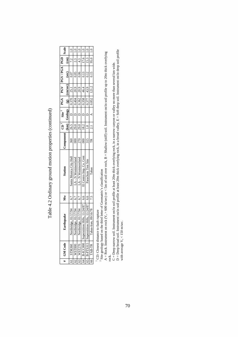
70
Tabl
e 4.
2 O
rdin
ary
grou
nd m
otio
n pr
oper
ties (
cont
inue
d)
1 CD
: Clo
sest
dis
tanc
e to
faul
t rup
ture
2 S
ite g
eolo
gy b
ased
on
the
third
lette
r of G
eom
atrix
’s c
lass
ifica
tion
A =
Roc
k. In
stru
men
t on
rock
(Vs >
600
m/s
ec) o
r < 5
m o
f soi
l ove
r roc
k, B
= S
hallo
w (s
tiff)
soil.
Inst
rum
ent o
n/in
soil
prof
ile u
p to
20m
thic
k ov
erly
ing
rock
. C
= D
eep
narr
ow so
il. In
stru
men
t on/
in so
il pr
ofile
at l
east
20m
thic
k ov
erly
ing
rock
, in
a na
rrow
can
yon
or v
alle
y no
mor
e th
an se
vera
l km
wid
e.
D =
Dee
p br
oad
soil.
Inst
rum
ent o
n/in
soil
prof
ile a
t lea
st 2
0m th
ick
over
lyin
g ro
ck, i
n a
broa
d va
lley,
E =
Sof
t dee
p so
il. In
stru
men
t on/
in d
eep
soil
prof
ile
with
ave
rage
Vs <
150
m/s
ec.
#G
M C
ode
Ear
thqu
ake
Mw
Stat
ion
Com
pone
nt C
D 1
(km
) S
ite 2
Geo
logy
PGA
(g
)PG
V
(cm
/sec
)PG
V /
PGA
(s
ec)
PGD
(c
m)
Scal
e
61ST
M36
0N
orth
ridge
, 01/
17/9
46.
7Sa
nta
Mon
ica
City
Hal
l36
026
.5D
0.37
025
.10.
077.
21.
062
WST
000
Nor
thrid
ge, 0
1/17
/94
6.7
LA -
N W
estm
orel
and
000
29.0
D0.
404
20.9
0.05
2.3
1.0
63W
ST27
0N
orth
ridge
, 01/
17/9
46.
7LA
- N
Wes
tmor
elan
d27
029
.0D
0.36
220
.90.
064.
31.
064
B-IC
C00
0Su
pers
titio
n H
ills,
11/2
4/87
6.6
El C
entro
Imp.
Co.
Cen
t00
018
.2D
0.35
846
.40.
1317
.61.
065
B-P
TS31
5Su
pers
titio
n H
ills,
11/2
4/87
6.6
Para
chut
e Te
st S
ite31
51.
0D
0.37
743
.90.
1215
.31.
066
TAB
-TR
Taba
s-Ira
n, 0
9/16
/78
7.5
Taba
sTR
2.1
A0.
852
121.
20.
1595
.01.
0
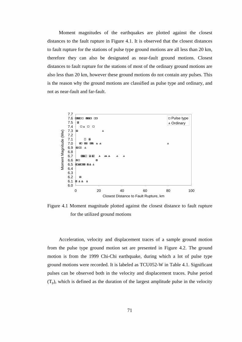
71
Moment magnitudes of the earthquakes are plotted against the closest
distances to the fault rupture in Figure 4.1. It is observed that the closest distances
to fault rupture for the stations of pulse type ground motions are all less than 20 km,
therefore they can also be designated as near-fault ground motions. Closest
distances to fault rupture for the stations of most of the ordinary ground motions are
also less than 20 km, however these ground motions do not contain any pulses. This
is the reason why the ground motions are classified as pulse type and ordinary, and
not as near-fault and far-fault.
Figure 4.1 Moment magnitude plotted against the closest distance to fault rupture
for the utilized ground motions
Acceleration, velocity and displacement traces of a sample ground motion
from the pulse type ground motion set are presented in Figure 4.2. The ground
motion is from the 1999 Chi-Chi earthquake, during which a lot of pulse type
ground motions were recorded. It is labeled as TCU052-W in Table 4.1. Significant
pulses can be observed both in the velocity and displacement traces. Pulse period
(Tp), which is defined as the duration of the largest amplitude pulse in the velocity
6.06.16.26.36.46.56.66.76.86.97.07.17.27.37.47.57.67.7
0 20 40 60 80 100Closest Distance to Fault Rupture, km
Mom
ent M
agni
tude
(Mw
)
Pulse typeOrdinary
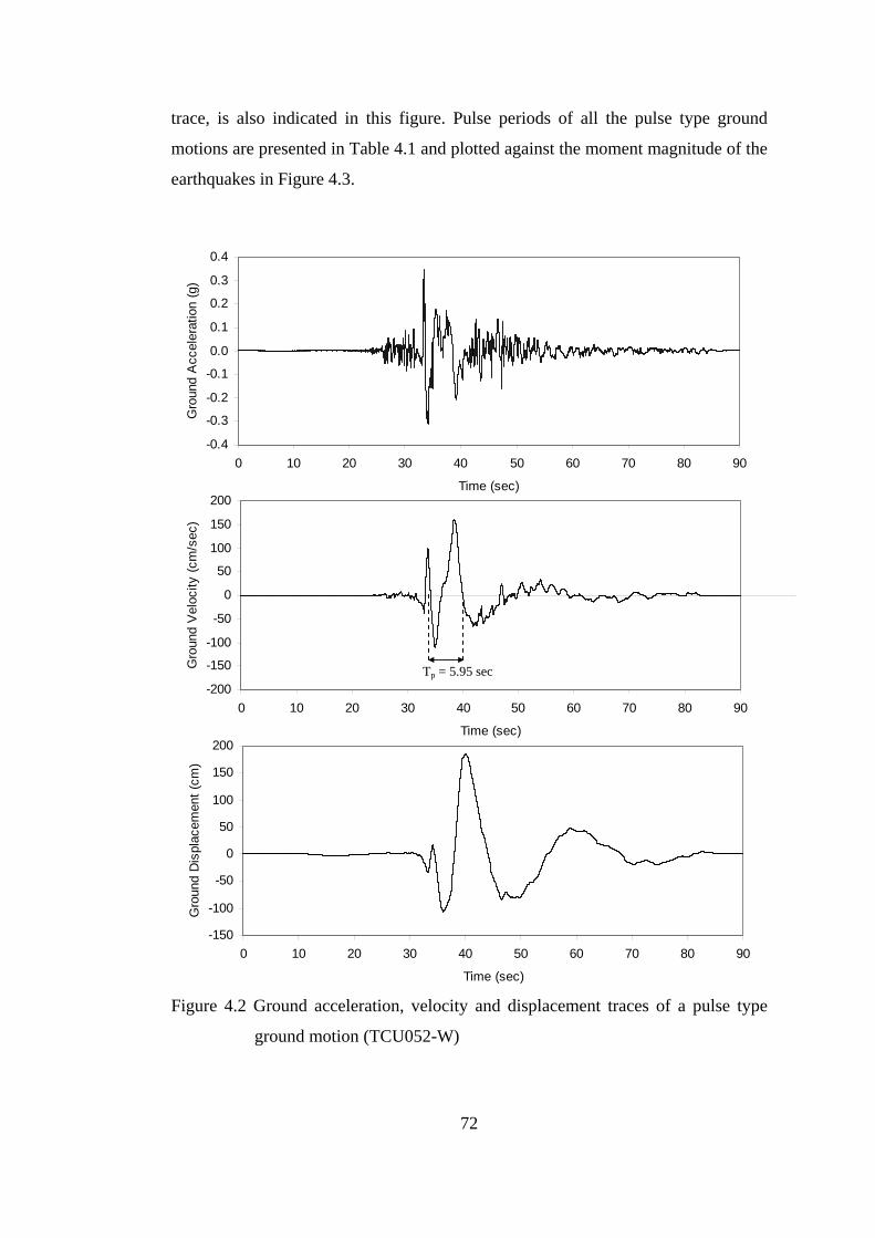
72
trace, is also indicated in this figure. Pulse periods of all the pulse type ground
motions are presented in Table 4.1 and plotted against the moment magnitude of the
earthquakes in Figure 4.3.
Figure 4.2 Ground acceleration, velocity and displacement traces of a pulse type
ground motion (TCU052-W)
-0.4
-0.3
-0.2
-0.1
0.0
0.1
0.2
0.3
0.4
0 10 20 30 40 50 60 70 80 90
Time (sec)
Gro
und
Acc
eler
atio
n (g
)
-150
-100
-50
0
50
100
150
200
0 10 20 30 40 50 60 70 80 90
Time (sec)
Gro
und
Dis
plac
emen
t (cm
)
-200
-150
-100
-50
0
50
100
150
200
0 10 20 30 40 50 60 70 80 90
Time (sec)
Gro
und
Vel
ocity
(cm
/sec
)
Tp = 5.95 sec
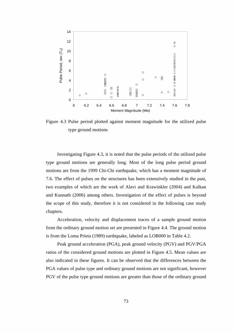
73
Figure 4.3 Pulse period plotted against moment magnitude for the utilized pulse
type ground motions
Investigating Figure 4.3, it is noted that the pulse periods of the utilized pulse
type ground motions are generally long. Most of the long pulse period ground
motions are from the 1999 Chi-Chi earthquake, which has a moment magnitude of
7.6. The effect of pulses on the structures has been extensively studied in the past,
two examples of which are the work of Alavi and Krawinkler (2004) and Kalkan
and Kunnath (2006) among others. Investigation of the effect of pulses is beyond
the scope of this study, therefore it is not considered in the following case study
chapters.
Acceleration, velocity and displacement traces of a sample ground motion
from the ordinary ground motion set are presented in Figure 4.4. The ground motion
is from the Loma Prieta (1989) earthquake, labeled as LOB000 in Table 4.2.
Peak ground acceleration (PGA), peak ground velocity (PGV) and PGV/PGA
ratios of the considered ground motions are plotted in Figure 4.5. Mean values are
also indicated in these figures. It can be observed that the differences between the
PGA values of pulse type and ordinary ground motions are not significant, however
PGV of the pulse type ground motions are greater than those of the ordinary ground
0
2
4
6
8
10
12
14
6 6.2 6.4 6.6 6.8 7 7.2 7.4 7.6 7.8Moment Magnitude (Mw)
Pul
se P
erio
d, s
ec (T
p)
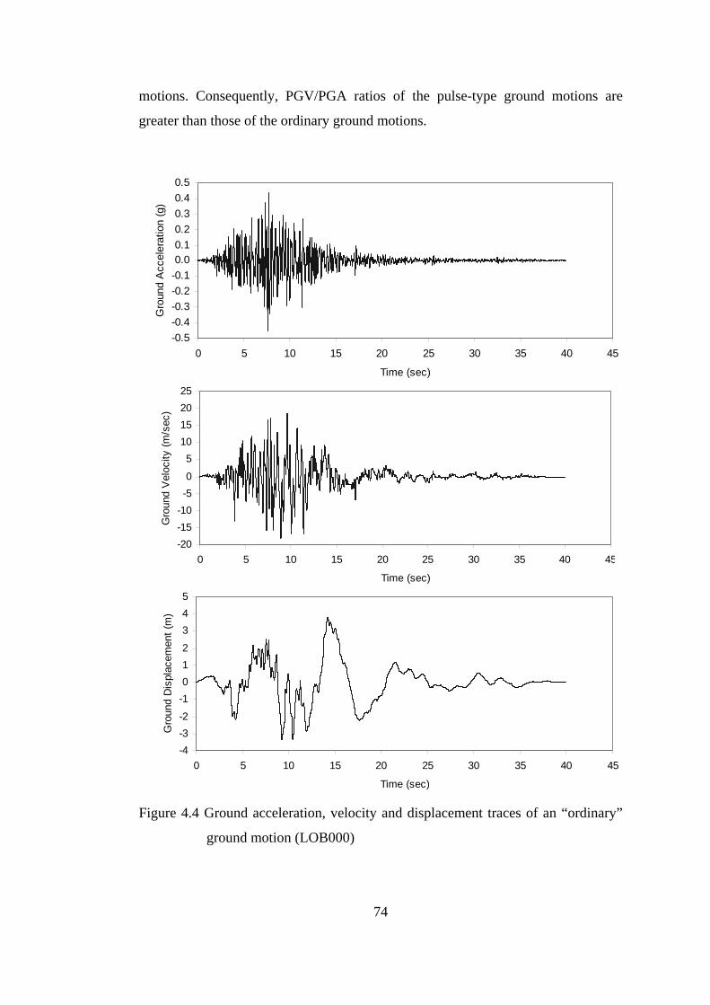
74
motions. Consequently, PGV/PGA ratios of the pulse-type ground motions are
greater than those of the ordinary ground motions.
Figure 4.4 Ground acceleration, velocity and displacement traces of an “ordinary”
ground motion (LOB000)
-0.5-0.4-0.3-0.2-0.10.00.10.20.30.40.5
0 5 10 15 20 25 30 35 40 45
Time (sec)
Gro
und
Acc
eler
atio
n (g
)
-20-15-10-50
510152025
0 5 10 15 20 25 30 35 40 45
Time (sec)
Gro
und
Vel
ocity
(m/s
ec)
-4-3-2
-1012
345
0 5 10 15 20 25 30 35 40 45
Time (sec)
Gro
und
Dis
plac
emen
t (m
)
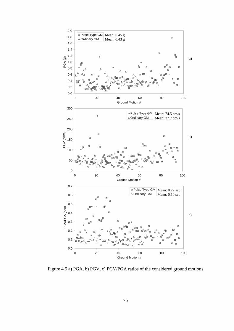
75
Figure 4.5 a) PGA, b) PGV, c) PGV/PGA ratios of the considered ground motions
0.0
0.2
0.4
0.6
0.8
1.0
1.2
1.4
1.6
1.8
2.0
0 20 40 60 80 100Ground Motion #
PG
A (g
)
Pulse Type GMOrdinary GM
a)
b)
c)
Mean: 0.45 g Mean: 0.43 g
0
50
100
150
200
250
300
0 20 40 60 80 100Ground Motion #
PG
V (c
m/s
)
Pulse Type GMOrdinary GM
Mean: 74.5 cm/s Mean: 37.7 cm/s
0.0
0.1
0.2
0.3
0.4
0.5
0.6
0.7
0 20 40 60 80 100Ground Motion #
PG
V/P
GA
(sec
)
Pulse Type GMOrdinary GM
Mean: 0.22 sec Mean: 0.10 sec
76
CHAPTER 5
CASE STUDY I:
TWELVE STORY RC PLANE FRAME
5.1 Description of the Building
The first case study is a twelve story reinforced concrete building with the
floor plan shown in Figure 5.1. The building is designed according to the
regulations of TS-500 (2000) and TEC (1998) in accordance with the capacity
design principles. An enhanced ductility level (R=8) is assumed for the building. It
is located in seismic zone 1 and the site class is Z3. Concrete and steel grades are
C25 and S420 respectively. Slab thickness for all floors is 14 cm and live load is 3.5
kN/m2. Dimensions of the beams at the first four, the second four and the last four
stories are 30x55, 30x50 and 30x45 cm2 respectively, whereas dimensions of the
columns at the first four, the second four and the last four stories are 60x60, 55x55
and 50x50 cm2 respectively. There is no basement, height of the ground story is 4 m
while the height of all other stories is 3.2 m. A plane model consisting of Frames A
and B is constructed for the analysis of the building (Figure 5.2).

77
Figure 5.1 Story plan of the twelve story building
Figure 5.2 Plane model of the twelve story building
6 m 4 m 6 m
5 m
5 m
5 m
Frame A
Frame B
6 m 4 m 6 m 6 m 4 m 6 m
Frame A Frame B
4 m
3.2 m
3.2 m
3.2 m
3.2 m
3.2 m
3.2 m
3.2 m
3.2 m
3.2 m
3.2 m
3.2 m
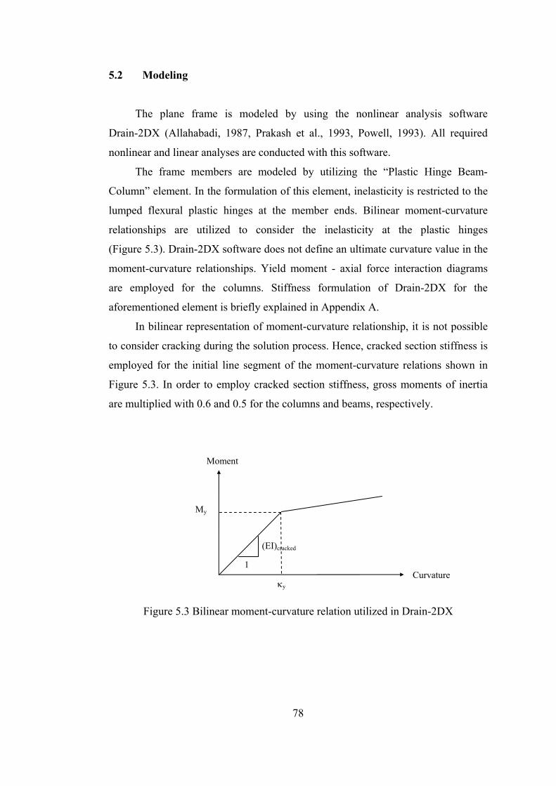
78
5.2 Modeling
The plane frame is modeled by using the nonlinear analysis software
Drain-2DX (Allahabadi, 1987, Prakash et al., 1993, Powell, 1993). All required
nonlinear and linear analyses are conducted with this software.
The frame members are modeled by utilizing the “Plastic Hinge Beam-
Column” element. In the formulation of this element, inelasticity is restricted to the
lumped flexural plastic hinges at the member ends. Bilinear moment-curvature
relationships are utilized to consider the inelasticity at the plastic hinges
(Figure 5.3). Drain-2DX software does not define an ultimate curvature value in the
moment-curvature relationships. Yield moment - axial force interaction diagrams
are employed for the columns. Stiffness formulation of Drain-2DX for the
aforementioned element is briefly explained in Appendix A.
In bilinear representation of moment-curvature relationship, it is not possible
to consider cracking during the solution process. Hence, cracked section stiffness is
employed for the initial line segment of the moment-curvature relations shown in
Figure 5.3. In order to employ cracked section stiffness, gross moments of inertia
are multiplied with 0.6 and 0.5 for the columns and beams, respectively.
Figure 5.3 Bilinear moment-curvature relation utilized in Drain-2DX
My
Curvature κy
Moment
(EI)cracked
1
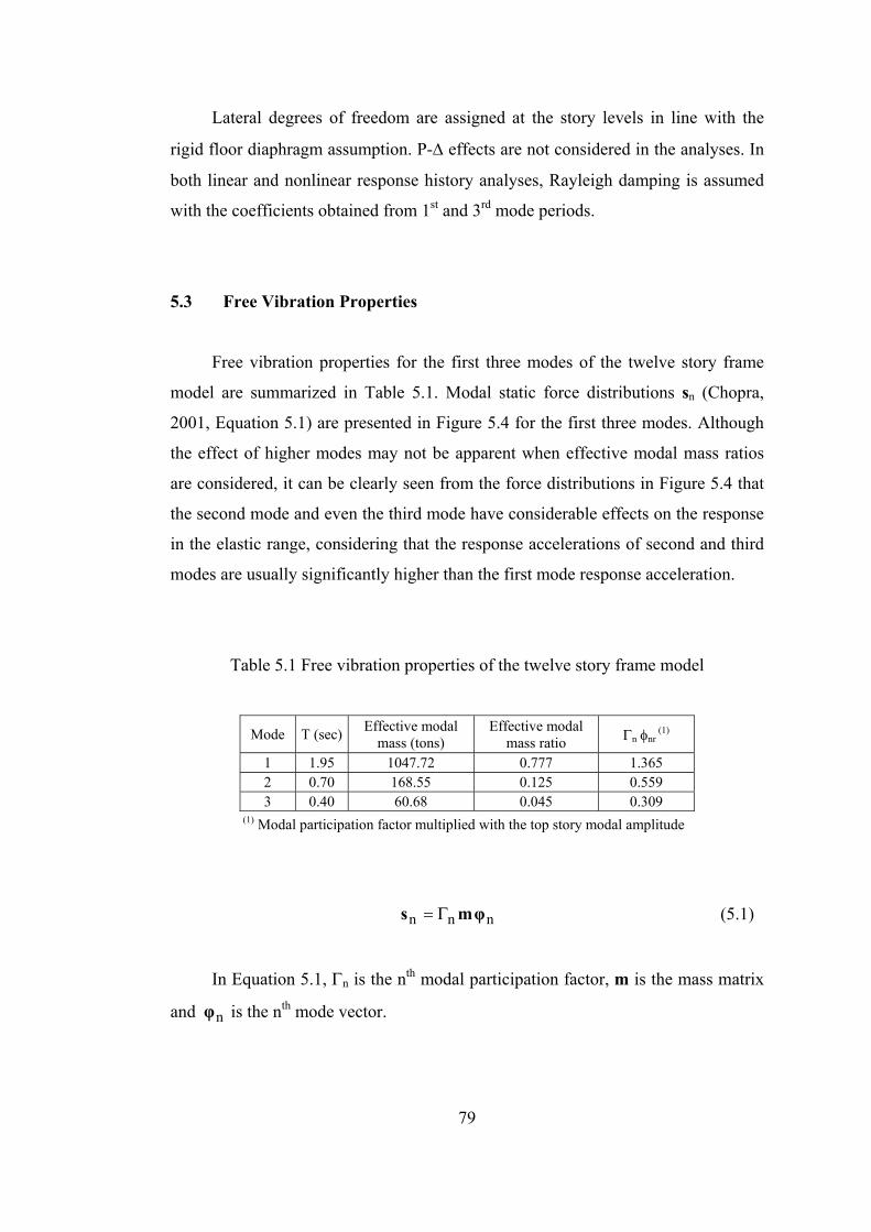
79
Lateral degrees of freedom are assigned at the story levels in line with the
rigid floor diaphragm assumption. P-Δ effects are not considered in the analyses. In
both linear and nonlinear response history analyses, Rayleigh damping is assumed
with the coefficients obtained from 1st and 3rd mode periods.
5.3 Free Vibration Properties
Free vibration properties for the first three modes of the twelve story frame
model are summarized in Table 5.1. Modal static force distributions sn (Chopra,
2001, Equation 5.1) are presented in Figure 5.4 for the first three modes. Although
the effect of higher modes may not be apparent when effective modal mass ratios
are considered, it can be clearly seen from the force distributions in Figure 5.4 that
the second mode and even the third mode have considerable effects on the response
in the elastic range, considering that the response accelerations of second and third
modes are usually significantly higher than the first mode response acceleration.
Table 5.1 Free vibration properties of the twelve story frame model
Mode T (sec) Effective modal mass (tons)
Effective modal mass ratio Γn φnr
(1)
1 1.95 1047.72 0.777 1.365 2 0.70 168.55 0.125 0.559 3 0.40 60.68 0.045 0.309
(1) Modal participation factor multiplied with the top story modal amplitude
nnn φms Γ= (5.1)
In Equation 5.1, Γn is the nth modal participation factor, m is the mass matrix
and nφ is the nth mode vector.
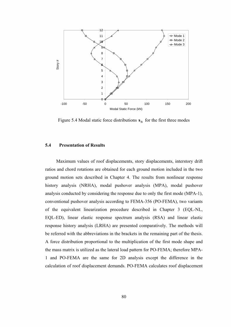
80
Figure 5.4 Modal static force distributions ns for the first three modes
5.4 Presentation of Results
Maximum values of roof displacements, story displacements, interstory drift
ratios and chord rotations are obtained for each ground motion included in the two
ground motion sets described in Chapter 4. The results from nonlinear response
history analysis (NRHA), modal pushover analysis (MPA), modal pushover
analysis conducted by considering the response due to only the first mode (MPA-1),
conventional pushover analysis according to FEMA-356 (PO-FEMA), two variants
of the equivalent linearization procedure described in Chapter 3 (EQL-NL,
EQL-ED), linear elastic response spectrum analysis (RSA) and linear elastic
response history analysis (LRHA) are presented comparatively. The methods will
be referred with the abbreviations in the brackets in the remaining part of the thesis.
A force distribution proportional to the multiplication of the first mode shape and
the mass matrix is utilized as the lateral load pattern for PO-FEMA; therefore MPA-
1 and PO-FEMA are the same for 2D analysis except the difference in the
calculation of roof displacement demands. PO-FEMA calculates roof displacement
0
1
2
3
4
5
6
7
8
9
10
11
12
-100 -50 0 50 100 150 200Modal Static Force (kN)
Sto
ry #
Mode 1Mode 2Mode 3
81
demand from the elastic spectral displacement of the first mode multiplied by a
series of coefficients to account for nonlinearity (Coefficient Method), while MPA-
1 calculates the roof displacement demand from the maximum displacement of an
equivalent inelastic SDOF system as explained in Chapter 2.
5.4.1 Description of Statistical Error Parameters
Three parameters are utilized in order to summarize the response statistics.
The first parameter is the median (xm), defined with Equation 5.2.
⎟⎟⎠
⎞⎜⎜⎝
⎛∑==
nxlnexpxn
1iim (5.2)
In Equation 5.2, n is the total number of data and xi is the ith individual data. xi
can be a response parameter obtained from nonlinear response history analysis or
from one of the approximate methods. It can also be a normalized value which is
obtained by dividing the considered response parameter found from an approximate
method by the one calculated with nonlinear response history analysis.
The second statistical parameter is the standard deviation σ in Equation 5.3.
21e2
μ⋅⎟⎠⎞
⎜⎝⎛ −=σ δ (5.3)
where
2
21
m exδ⋅
⋅=μ (5.4)
and
( ) ( )5.0n
1i
2mi 1nxlnxln ⎟⎟
⎠
⎞⎜⎜⎝
⎛−∑ −=δ
= (5.5)
82
μ in Equation 5.4 is the mean value of a lognormal variable and δ in Equation
5.5 is the dispersion (Benjamin and Cornell, 1970).
Median is often used to indicate the central value of a log-normal variable.
Standard deviation defined in Equation 5.3 also belongs to a variable sampled from
lognormal distribution (Ang and Tang, 1975). Lognormal distribution is suitable for
the maximum values of earthquake response parameters since they are always
positive.
Median and standard deviation are good indicators for evaluating the accuracy
of the approximate methods with respect to the nonlinear response history analysis,
which is used as benchmark. However, since these two parameters may result in
different combinations (median may be close to 1 whereas dispersion may be high
or vice versa), a third parameter, root mean square error (RMSE), is utilized for
comparing the relative accuracy of approximate methods (Equation 5.6).
( )
m
5.0n
1i
2ii
x
nx'xRMSE
⎟⎟⎠
⎞⎜⎜⎝
⎛∑ −
= = (5.6)
In Equation 5.6, i'x is the response parameter obtained from the approximate
method, ix is the response parameter obtained from nonlinear response history
analysis and xm is the median for x. The numerator can be interpreted as the average
error. Actually, numerator is sufficient in order to evaluate the accuracy of the
approximate methods with respect to each other. It is divided by the median here for
normalization. Thus the error is represented as a percentage. It should be noted that
RMSE can take values greater than 1.0.
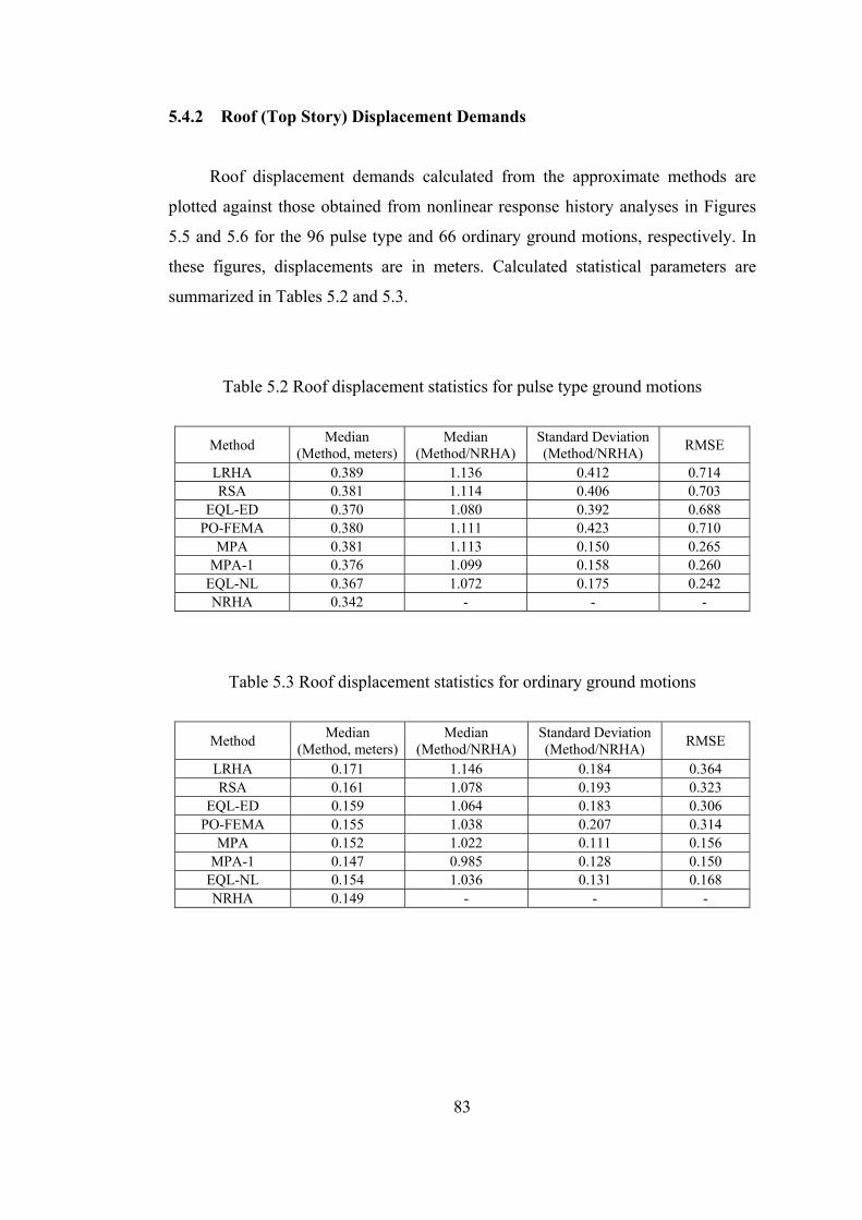
83
5.4.2 Roof (Top Story) Displacement Demands
Roof displacement demands calculated from the approximate methods are
plotted against those obtained from nonlinear response history analyses in Figures
5.5 and 5.6 for the 96 pulse type and 66 ordinary ground motions, respectively. In
these figures, displacements are in meters. Calculated statistical parameters are
summarized in Tables 5.2 and 5.3.
Table 5.2 Roof displacement statistics for pulse type ground motions
Method Median
(Method, meters)Median
(Method/NRHA) Standard Deviation (Method/NRHA) RMSE
LRHA 0.389 1.136 0.412 0.714 RSA 0.381 1.114 0.406 0.703
EQL-ED 0.370 1.080 0.392 0.688 PO-FEMA 0.380 1.111 0.423 0.710
MPA 0.381 1.113 0.150 0.265 MPA-1 0.376 1.099 0.158 0.260
EQL-NL 0.367 1.072 0.175 0.242 NRHA 0.342 - - -
Table 5.3 Roof displacement statistics for ordinary ground motions
Method Median
(Method, meters)Median
(Method/NRHA) Standard Deviation (Method/NRHA) RMSE
LRHA 0.171 1.146 0.184 0.364 RSA 0.161 1.078 0.193 0.323
EQL-ED 0.159 1.064 0.183 0.306 PO-FEMA 0.155 1.038 0.207 0.314
MPA 0.152 1.022 0.111 0.156 MPA-1 0.147 0.985 0.128 0.150
EQL-NL 0.154 1.036 0.131 0.168 NRHA 0.149 - - -
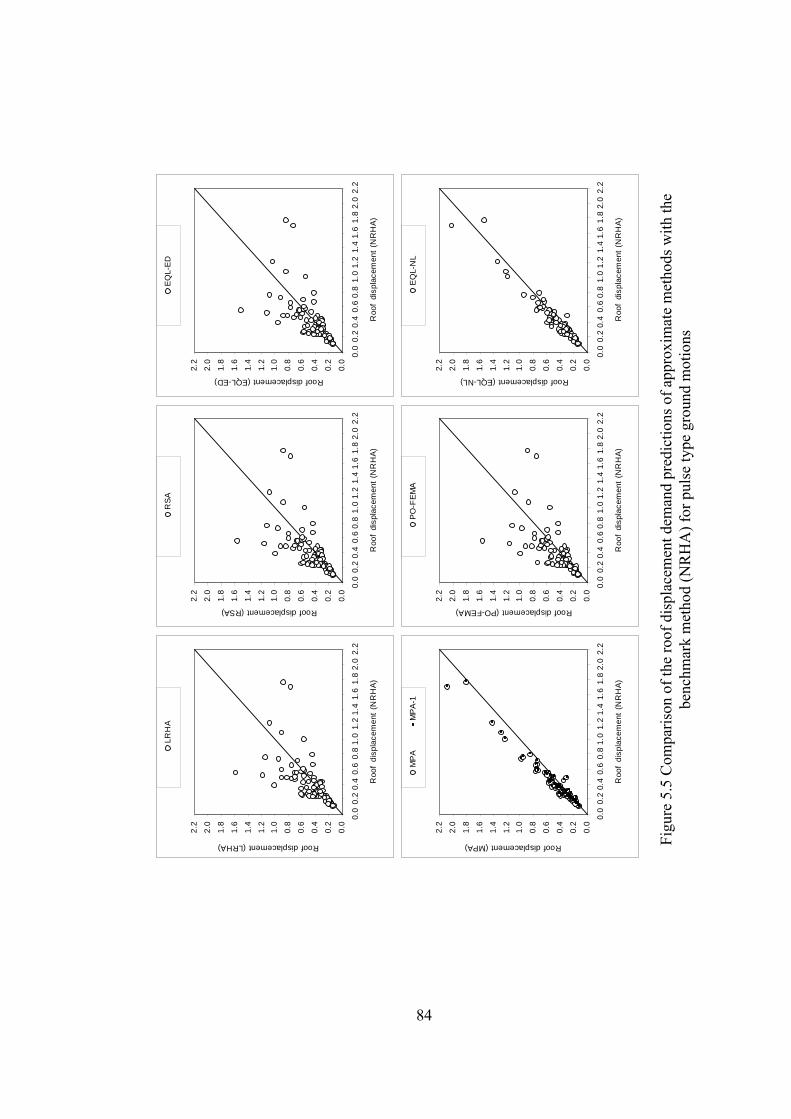
84
Figu
re 5
.5 C
ompa
rison
of t
he ro
of d
ispl
acem
ent d
eman
d pr
edic
tions
of a
ppro
xim
ate
met
hods
with
the
benc
hmar
k m
etho
d (N
RH
A) f
or p
ulse
type
gro
und
mot
ions
0.0
0.2
0.4
0.6
0.8
1.0
1.2
1.4
1.6
1.8
2.0
2.2
0.0
0.2
0.4
0.6
0.8
1.0
1.2
1.4
1.6
1.8
2.0
2.2
Roo
f di
spla
cem
ent
(NR
HA
)
Roof displacement (LRHA)
LRH
A
0.0
0.2
0.4
0.6
0.8
1.0
1.2
1.4
1.6
1.8
2.0
2.2
0.0
0.2
0.4
0.6
0.8
1.0
1.2
1.4
1.6
1.8
2.0
2.2
Roo
f di
spla
cem
ent
(NR
HA
)
Roof displacement (RSA)
RSA
0.0
0.2
0.4
0.6
0.8
1.0
1.2
1.4
1.6
1.8
2.0
2.2
0.0
0.2
0.4
0.6
0.8
1.0
1.2
1.4
1.6
1.8
2.0
2.2
Roo
f di
spla
cem
ent (
NR
HA
)
Roof displacement (EQL-ED)
EQ
L-E
D
0.0
0.2
0.4
0.6
0.8
1.0
1.2
1.4
1.6
1.8
2.0
2.2
0.0
0.2
0.4
0.6
0.8
1.0
1.2
1.4
1.6
1.8
2.0
2.2
Roo
f di
spla
cem
ent
(NR
HA
)
Roof displacement (MPA)
MP
AM
PA
-1
0.0
0.2
0.4
0.6
0.8
1.0
1.2
1.4
1.6
1.8
2.0
2.2
0.0
0.2
0.4
0.6
0.8
1.0
1.2
1.4
1.6
1.8
2.0
2.2
Roo
f di
spla
cem
ent
(NR
HA
)
Roof displacement (PO-FEMA)
PO
-FE
MA
0.0
0.2
0.4
0.6
0.8
1.0
1.2
1.4
1.6
1.8
2.0
2.2
0.0
0.2
0.4
0.6
0.8
1.0
1.2
1.4
1.6
1.8
2.0
2.2
Roo
f di
spla
cem
ent (
NR
HA
)
Roof displacement (EQL-NL)
EQ
L-N
L
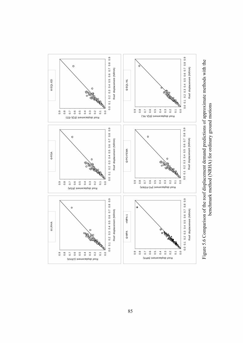
85
Figu
re 5
.6 C
ompa
rison
of t
he ro
of d
ispl
acem
ent d
eman
d pr
edic
tions
of a
ppro
xim
ate
met
hods
with
the
benc
hmar
k m
etho
d (N
RH
A) f
or o
rdin
ary
grou
nd m
otio
ns
0.0
0.1
0.2
0.3
0.4
0.5
0.6
0.7
0.8
0.9
0.0
0.1
0.2
0.3
0.4
0.5
0.6
0.7
0.8
0.9
Roo
f di
spla
cem
ent (
NR
HA)
Roof displacement (EQL-ED)
EQ
L-E
D
0.0
0.1
0.2
0.3
0.4
0.5
0.6
0.7
0.8
0.9
0.0
0.1
0.2
0.3
0.4
0.5
0.6
0.7
0.8
0.9
Roo
f di
spla
cem
ent
(NR
HA
)
Roof displacement (RSA)
RSA
0.0
0.1
0.2
0.3
0.4
0.5
0.6
0.7
0.8
0.9
0.0
0.1
0.2
0.3
0.4
0.5
0.6
0.7
0.8
0.9
Roo
f di
spla
cem
ent
(NR
HA
)
Roof displacement (LRHA)
LRH
A
0.0
0.1
0.2
0.3
0.4
0.5
0.6
0.7
0.8
0.9
0.0
0.1
0.2
0.3
0.4
0.5
0.6
0.7
0.8
0.9
Roo
f di
spla
cem
ent
(NR
HA
)
Roof displacement (MPA)
MP
AM
PA-1
0.0
0.1
0.2
0.3
0.4
0.5
0.6
0.7
0.8
0.9
0.0
0.1
0.2
0.3
0.4
0.5
0.6
0.7
0.8
0.9
Roo
f di
spla
cem
ent (
NR
HA)
Roof displacement (PO-FEMA)
PO
-FE
MA
0.0
0.1
0.2
0.3
0.4
0.5
0.6
0.7
0.8
0.9
0.0
0.1
0.2
0.3
0.4
0.5
0.6
0.7
0.8
0.9
Roo
f di
spla
cem
ent
(NR
HA
)
Roof displacement (EQL-NL)
EQ
L-N
L
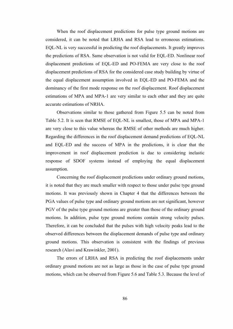
86
When the roof displacement predictions for pulse type ground motions are
considered, it can be noted that LRHA and RSA lead to erroneous estimations.
EQL-NL is very successful in predicting the roof displacements. It greatly improves
the predictions of RSA. Same observation is not valid for EQL-ED. Nonlinear roof
displacement predictions of EQL-ED and PO-FEMA are very close to the roof
displacement predictions of RSA for the considered case study building by virtue of
the equal displacement assumption involved in EQL-ED and PO-FEMA and the
dominancy of the first mode response on the roof displacement. Roof displacement
estimations of MPA and MPA-1 are very similar to each other and they are quite
accurate estimations of NRHA.
Observations similar to those gathered from Figure 5.5 can be noted from
Table 5.2. It is seen that RMSE of EQL-NL is smallest, those of MPA and MPA-1
are very close to this value whereas the RMSE of other methods are much higher.
Regarding the differences in the roof displacement demand predictions of EQL-NL
and EQL-ED and the success of MPA in the predictions, it is clear that the
improvement in roof displacement prediction is due to considering inelastic
response of SDOF systems instead of employing the equal displacement
assumption.
Concerning the roof displacement predictions under ordinary ground motions,
it is noted that they are much smaller with respect to those under pulse type ground
motions. It was previously shown in Chapter 4 that the differences between the
PGA values of pulse type and ordinary ground motions are not significant, however
PGV of the pulse type ground motions are greater than those of the ordinary ground
motions. In addition, pulse type ground motions contain strong velocity pulses.
Therefore, it can be concluded that the pulses with high velocity peaks lead to the
observed differences between the displacement demands of pulse type and ordinary
ground motions. This observation is consistent with the findings of previous
research (Alavi and Krawinkler, 2001).
The errors of LRHA and RSA in predicting the roof displacements under
ordinary ground motions are not as large as those in the case of pulse type ground
motions, which can be observed from Figure 5.6 and Table 5.3. Because the level of
87
nonlinearity is lower for ordinary ground motions with respect to the pulse type
ground motions. EQL-NL improves RSA predictions and reduces the error to the
half of RSA for ordinary ground motions. Improvement in the predictions can also
be observed from Figure 5.6. Like the case of pulse type ground motions, LRHA,
RSA, EQL-ED and PO-FEMA predictions are similar to each other. Estimations of
MPA and MPA-1 are very close to each other and accurate as in the case of pulse
type ground motions.
5.4.3 Local Response Parameters
Comparison of story displacements, interstory drift ratios, beam chord
rotations and column chord rotations obtained from the previously mentioned
analysis methods are presented in this section. For this purpose, ground motions
producing NRHA roof displacements between 0.140 m (0.36 % roof drift) and
1.250 m (3.2 % roof drift) are taken into consideration. Lower bound corresponds to
the onset of inelasticity. An upper bound is also set because P-Δ effects are not
considered and ultimate curvature values are not utilized in the moment curvature
relations. The number of pulse type and ordinary ground motions remaining in
between the aforementioned bounds are 79 and 31, respectively. Roof displacement
demands of these ground motions normalized by the building height are marked on
the first mode pushover curve of the building in Figure 5.7. Roof displacements
obtained from the pulse type ground motions cover a wider range and they are
larger than those obtained from ordinary ground motions.
Base shear capacity prediction of the equivalent linearization procedure is
also shown with a horizontal line in Figure 5.7. It can be observed that this value is
close to the one obtained from pushover analysis. It should be noted that the
maximum base shear values obtained from nonlinear response history analyses are
different than the values on the pushover curve; therefore ordinates of the marked
points in Figure 5.7 are not the actual values.

88
Figure 5.7 Roof displacement demands obtained from a) pulse type ground motions,
b) ordinary ground motions marked on the first mode pushover curve
Pseudo acceleration and displacement response spectra of the 79 pulse type
and 31 ordinary ground motions are plotted in Figures 5.8 and 5.9, respectively. It
can be observed that the displacements and pseudo accelerations corresponding to
the second and third mode periods can be regarded as similar for pulse type and
ordinary ground motions, whereas those corresponding to the first mode period are
much greater for pulse type ground motions with respect to the ordinary ground
motions. This observation indicates that higher mode effects are more distinct in the
elastic range for ordinary ground motions than the pulse type ground motions.
a)
b)
0
0.02
0.04
0.06
0.08
0.1
0.12
0 0.005 0.01 0.015 0.02 0.025 0.03 0.035Roof Displacement / Building Height
Bas
e S
hear
/ W
eigh
t
Pushover Curve
Pulse Type Ground Motions
Equivalent Linearization MethodBase Shear Capacity Prediction
0
0.02
0.04
0.06
0.08
0.1
0.12
0 0.005 0.01 0.015 0.02 0.025 0.03 0.035Roof Displacement / Building Height
Bas
e S
hear
/ W
eigh
t
Pushover Curve
Ordinary Ground Motions
Equivalent Linearization MethodBase Shear Capacity Prediction
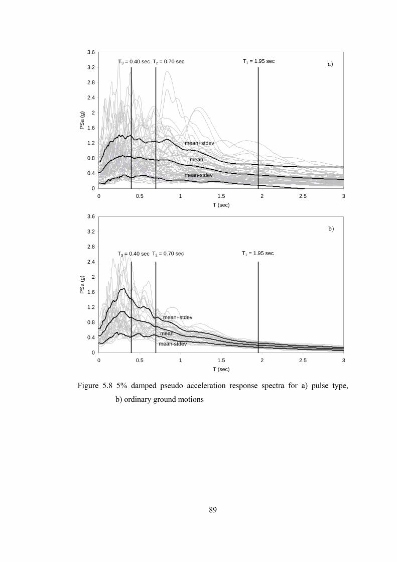
89
Figure 5.8 5% damped pseudo acceleration response spectra for a) pulse type,
b) ordinary ground motions
0
0.4
0.8
1.2
1.6
2
2.4
2.8
3.2
3.6
0 0.5 1 1.5 2 2.5 3T (sec)
PS
a (g
)
mean
mean+stdev
mean-stdev
T1 = 1.95 secT2 = 0.70 secT3 = 0.40 sec
0
0.4
0.8
1.2
1.6
2
2.4
2.8
3.2
3.6
0 0.5 1 1.5 2 2.5 3T (sec)
PS
a (g
)
mean
mean+stdev
mean-stdev
T1 = 1.95 secT2 = 0.70 secT3 = 0.40 sec
a)
b)
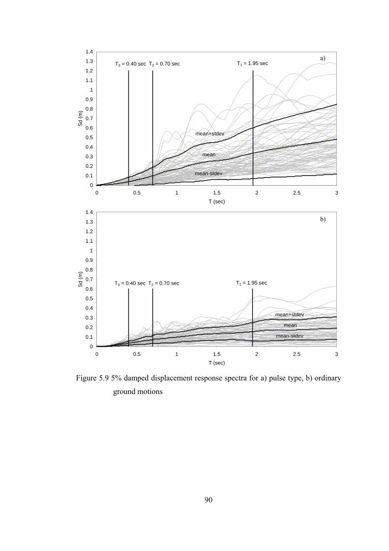
90
Figure 5.9 5% damped displacement response spectra for a) pulse type, b) ordinary
ground motions
0
0.1
0.2
0.3
0.4
0.5
0.6
0.7
0.8
0.9
1
1.1
1.2
1.3
1.4
0 0.5 1 1.5 2 2.5 3T (sec)
Sd
(m)
mean
mean+stdev
mean-stdev
T1 = 1.95 secT2 = 0.70 secT3 = 0.40 sec
0
0.1
0.2
0.3
0.4
0.5
0.6
0.7
0.8
0.9
1
1.1
1.2
1.3
1.4
0 0.5 1 1.5 2 2.5 3T (sec)
Sd
(m)
mean
mean+stdev
mean-stdev
T1 = 1.95 secT2 = 0.70 secT3 = 0.40 seca)
b)
91
Roof displacement comparisons were presented in the previous section and it
was observed that the roof displacement predictions of the approximate methods
were generally larger than those of the benchmark method (NRHA) by different
amounts ranging from 12 to 15 percent at the medial level. Although all of the
considered approximate methods have their own ways of calculating a roof
displacement demand, comparison of local response parameters is conducted such
that each approximate method is assumed to calculate the same roof displacement
with NRHA. The purpose for such an adjustment is to observe the accuracy of the
approximate methods in estimating the distribution of local response parameters
within the structure. Otherwise, as it will be demonstrated later, inaccurate
calculation of roof displacements may result in accurate estimations of some local
response parameters by coincidence. This comparison strategy was previously
employed in FEMA-440 (ATC, 2005). In the case of equating the roof
displacements of the approximate methods to that of NRHA, there remains no
difference between the methods MPA-1 and PO-FEMA and small difference
between EQL-NL and EQL-ED. Therefore, PO-FEMA and EQL-ED results are not
presented for further evaluations. For equating the roof displacement to that of
NRHA, first mode pushover analysis is conducted with a target displacement equal
to the NRHA roof displacement in MPA-1. Modal displacements calculated by
MPA, variants of the equivalent linearization procedure and RSA are scaled with
the ratio of the NRHA roof displacement to the roof displacement predicted by the
approximate method. Response parameters obtained from LRHA are multiplied
with the ratio of the roof displacement demand of NRHA to that of LRHA.
Median and RMSE of story displacements, interstory drift ratios, beam chord
rotations and column chord rotations obtained from the employed analysis methods
are plotted in Figures 5.10-5.13 for pulse type ground motions. For each method
and each ground motion, the maximum value of a response parameter is obtained,
and then the statistical parameters are calculated for each method by using all the
ground motions in the set. It should be noted that, for a ground motion, the
maximum values of different response parameters are obtained at different times in
response history analyses. Beam chord rotation at a story level indicates the average
92
of the chord rotations at the beam ends at a story level. Similarly, column bottom
end chord rotation indicates the average of the chord rotations at the bottom ends of
the columns at a story. Column top end chord rotations are not shown since upper
ends of the columns remain in the elastic range and their median chord rotations do
not exceed 0.0025 radians.
Interstory drift ratios obtained from the approximate methods divided by
those obtained from NRHA are plotted in Figure 5.14 for pulse type ground
motions. In this figure, each thin gray line corresponds to a ground motion and the
thick gray lines indicate the median minus standard deviation, median and median
plus standard deviation values. Beam chord rotations produce almost exactly the
same figures, hence they are not presented herein. Following observations can be
made from Figures 5.10-5.14.
• Equivalent linearization procedure significantly improves the response
predictions of RSA. Improvement is substantial for the interstory drift ratios
and beam chord rotations, those especially at the upper stories. RSA greatly
overestimates the beam chord rotations and interstory drift ratios at the upper
stories. Equivalent linearization procedure is successful in bringing these
values closer to NRHA results.
• RMSE of column bottom end chord rotations of the first story obtained from
RSA is reduced slightly by the equivalent linearization procedure. RMSE of
the column bottom end chord rotations of the above stories do not possess a
practical importance since they remain in the elastic range.
• Differences in the median and RMSE values of RSA and LRHA are due to
the SRSS combination rule. In general, responses obtained from RSA and
LRHA are similar (Figure 5.14). Therefore, errors resulting from SRSS
combination can be considered to be at an acceptable level.
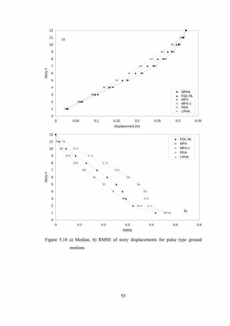
93
Figure 5.10 a) Median, b) RMSE of story displacements for pulse type ground
motions
0
1
2
3
4
5
6
7
8
9
10
11
12
0 0.1 0.2 0.3 0.4 0.5 0.6
RMSE
Sto
ry #
EQL-NLMPAMPA-1RSALRHA
0
1
2
3
4
5
6
7
8
9
10
11
12
0 0.05 0.1 0.15 0.2 0.25 0.3 0.35
Displacement (m)
Sto
ry #
NRHAEQL-NLMPAMPA-1RSALRHA
b)
a)
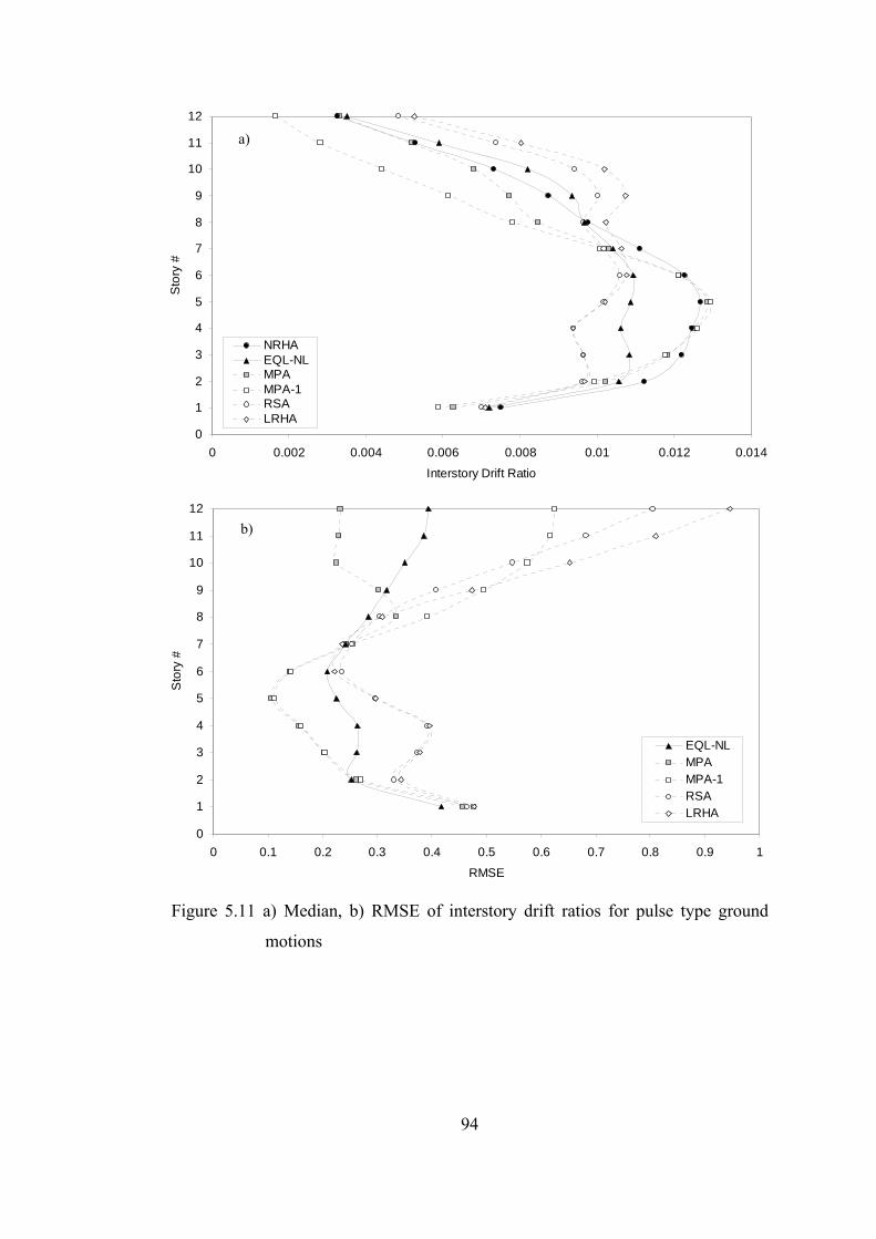
94
Figure 5.11 a) Median, b) RMSE of interstory drift ratios for pulse type ground
motions
0
1
2
3
4
5
6
7
8
9
10
11
12
0 0.1 0.2 0.3 0.4 0.5 0.6 0.7 0.8 0.9 1
RMSE
Sto
ry #
EQL-NLMPAMPA-1RSALRHA
0
1
2
3
4
5
6
7
8
9
10
11
12
0 0.002 0.004 0.006 0.008 0.01 0.012 0.014
Interstory Drift Ratio
Sto
ry #
NRHAEQL-NLMPAMPA-1RSALRHA
b)
a)
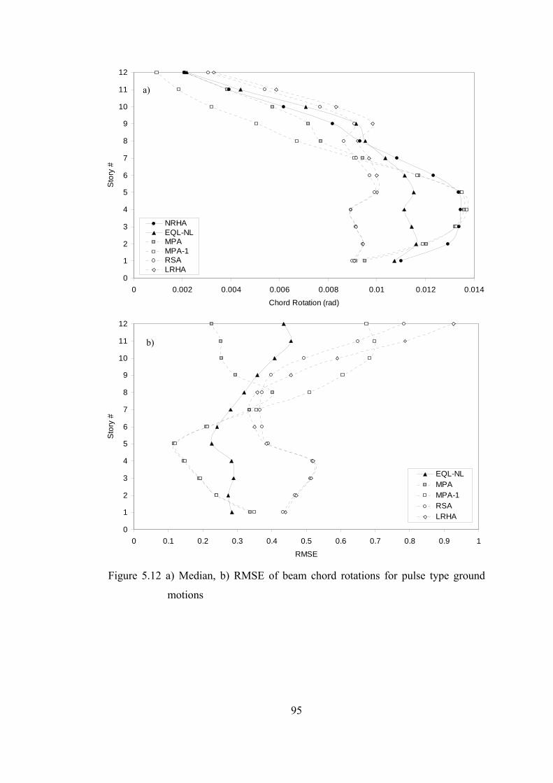
95
Figure 5.12 a) Median, b) RMSE of beam chord rotations for pulse type ground
motions
0
1
2
3
4
5
6
7
8
9
10
11
12
0 0.1 0.2 0.3 0.4 0.5 0.6 0.7 0.8 0.9 1
RMSE
Sto
ry #
EQL-NLMPAMPA-1RSALRHA
0
1
2
3
4
5
6
7
8
9
10
11
12
0 0.002 0.004 0.006 0.008 0.01 0.012 0.014
Chord Rotation (rad)
Sto
ry #
NRHAEQL-NLMPAMPA-1RSALRHA
b)
a)
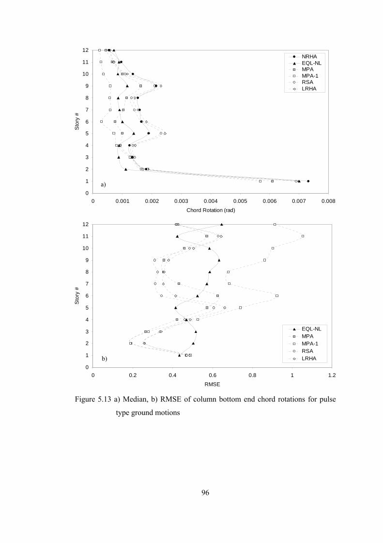
96
Figure 5.13 a) Median, b) RMSE of column bottom end chord rotations for pulse
type ground motions
0
1
2
3
4
5
6
7
8
9
10
11
12
0 0.2 0.4 0.6 0.8 1 1.2
RMSE
Sto
ry #
EQL-NLMPAMPA-1RSALRHA
0
1
2
3
4
5
6
7
8
9
10
11
12
0 0.001 0.002 0.003 0.004 0.005 0.006 0.007 0.008
Chord Rotation (rad)
Sto
ry #
NRHAEQL-NLMPAMPA-1RSALRHA
b)
a)
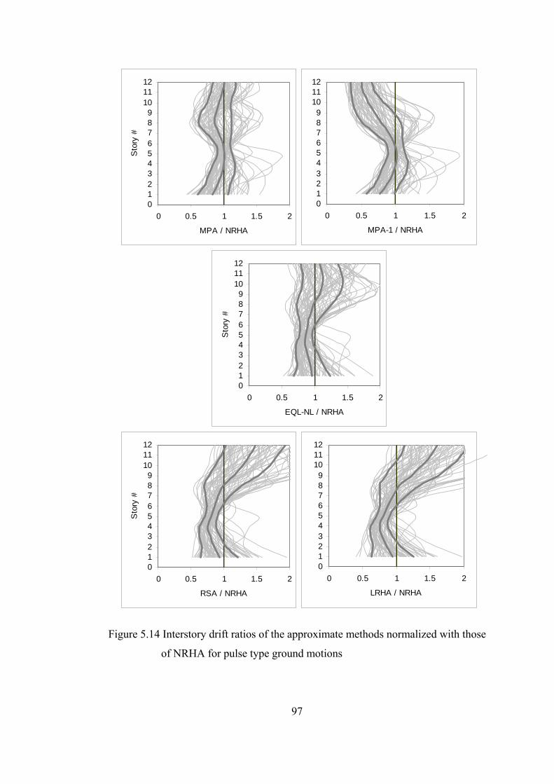
97
Figure 5.14 Interstory drift ratios of the approximate methods normalized with those
of NRHA for pulse type ground motions
0123456789
101112
0 0.5 1 1.5 2
EQL-NL / NRHA
Sto
ry #
0123456789
101112
0 0.5 1 1.5 2
MPA / NRHA
Sto
ry #
0123456789
101112
0 0.5 1 1.5 2
MPA-1 / NRHA
0123456789
101112
0 0.5 1 1.5 2
RSA / NRHA
Sto
ry #
0123456789
101112
0 0.5 1 1.5 2
LRHA / NRHA
98
• When the distribution of median interstory drift ratios along the building
height obtained from LRHA and NRHA are compared (Figure 5.11a), it can
be seen that higher mode effects are less apparent in NRHA with respect to
LRHA. This situation is due to the fact that; although higher mode forces in
the elastic range tend to induce inelasticity at the upper parts, their effects
decrease after the onset of yielding at the bottom stories and inelasticity can
not increase further at the upper stories as much as at the lower stories.
• The decrease in the effect of higher mode forces in the inelastic range may be
explained by inspection of the pseudo acceleration response spectra in Figure
5.8. After the onset of yielding in structural members, natural periods of the
structure elongate. Increase in the first mode period does not result in a
significant change in pseudo acceleration. However, pseudo accelerations of
the second and third modes decrease with respect to the elastic mode periods.
Since the second and third mode pseudo accelerations decrease and first mode
pseudo acceleration does not change significantly, effect of higher modes
decrease in the inelastic range.
• Investigating the distribution of median interstory drift ratios and beam chord
rotations along the height (Figures 5.11a and 5.12a), it is observed that
reduction in the higher mode effects is captured by the equivalent
linearization procedure.
• MPA is successful in correcting the interstory drift ratios and beam chord
rotations at the upper stories predicted by the first mode pushover analysis
(MPA-1). It possesses much lower RMSE values with respect to MPA-1 and
results in very close median response to NRHA median at the upper three
stories. However, it is ineffective in reducing the RMSE of first story column
bottom end chord rotations. Both MPA and MPA-1 underestimate the median
column bottom end chord rotations of the first story.
• In comparison with the approximate nonlinear analysis methods, RMSE of the
equivalent linearization procedure is generally larger than RMSE of MPA,
however differences are not significant. Error of the equivalent linearization
99
procedure is smaller than MPA-1 at the upper stories, which is an indication
of the ability of the procedure in capturing the higher mode effects.
Median and RMSE of story displacements, interstory drift ratios, beam chord
rotations and column chord rotations obtained from the employed analysis methods
are plotted in Figures 5.15-5.18 for ordinary ground motions. Column top end chord
rotations are not shown in these figures since upper ends of the columns remain in
the elastic range and their median chord rotations do not exceed 0.002 radians.
Interstory drift ratios of the approximate methods divided by those of NRHA
are plotted in Figure 5.19. In this figure, each thin gray line corresponds to a ground
motion and the thick gray lines indicate the median-standard deviation, median and
median+standard deviation values. The following observations can be made from
Figures 5.15-5.19.
• Similar to the case of pulse type ground motions, it is observed that equivalent
linearization procedure improves the response predictions of RSA. RSA
overestimates beam chord rotations and interstory drift ratios at the upper
stories. Equivalent linearization procedure is successful at bringing these
values closer to NRHA results.
• RMSE of column bottom end chord rotations is similar for all of the
approximate methods. RMSE of the column bottom end chord rotations of the
2nd and upper stories do not possess a practical importance since they remain
in the elastic range.
• Observing the distribution of median interstory drift ratios along the height, it
is noted that reduction in the higher mode effects between LRHA and NRHA
is less pronounced for ordinary ground motions compared to pulse type
ground motions. Ordinary ground motions result in lower levels of
nonlinearity, which consequently results in smaller amounts of period
elongation. Therefore the effect of higher modes does not reduce in the
inelastic range for ordinary ground motions as much as the case of pulse type
ground motions. In addition, it is also observed that higher mode effect
present in NRHA is noticed by the equivalent linearization procedure.
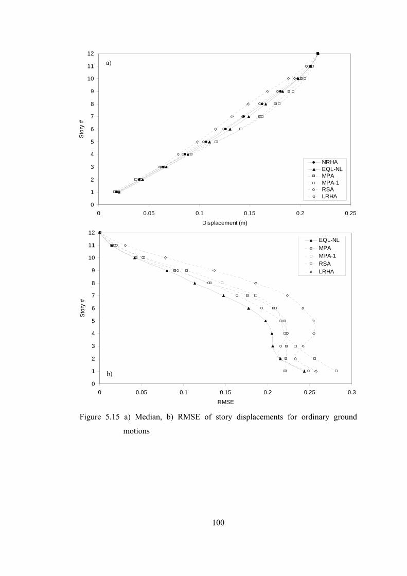
100
Figure 5.15 a) Median, b) RMSE of story displacements for ordinary ground
motions
0
1
2
3
4
5
6
7
8
9
10
11
12
0 0.05 0.1 0.15 0.2 0.25 0.3
RMSE
Sto
ry #
EQL-NLMPAMPA-1RSALRHA
0
1
2
3
4
5
6
7
8
9
10
11
12
0 0.05 0.1 0.15 0.2 0.25
Displacement (m)
Sto
ry #
NRHAEQL-NLMPAMPA-1RSALRHA
a)
b)
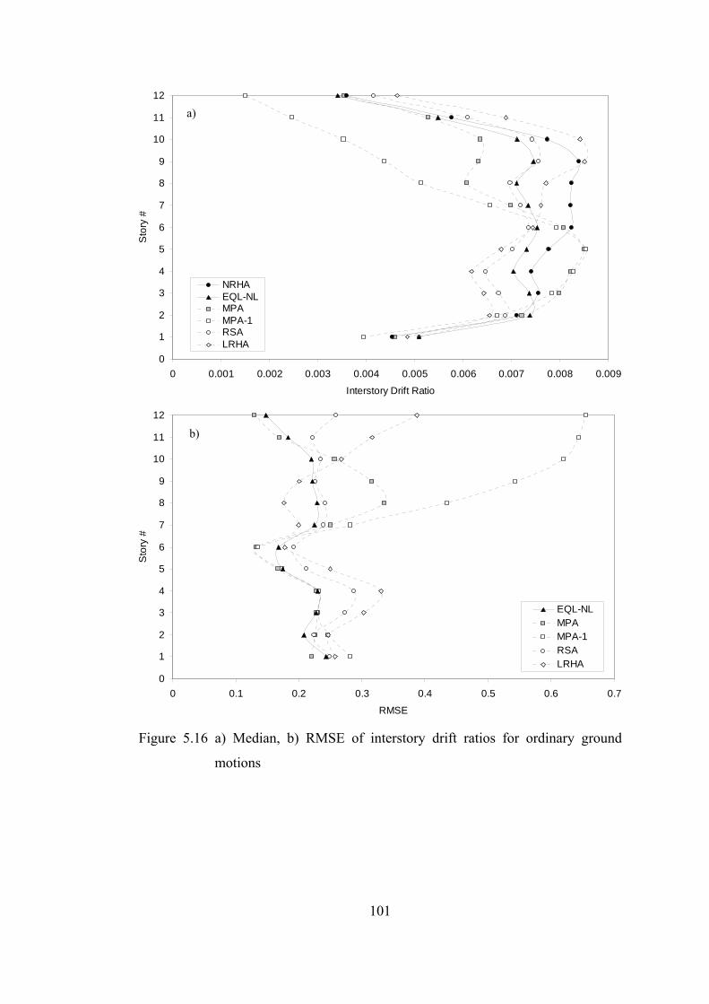
101
Figure 5.16 a) Median, b) RMSE of interstory drift ratios for ordinary ground
motions
0
1
2
3
4
5
6
7
8
9
10
11
12
0 0.1 0.2 0.3 0.4 0.5 0.6 0.7
RMSE
Sto
ry #
EQL-NLMPAMPA-1RSALRHA
0
1
2
3
4
5
6
7
8
9
10
11
12
0 0.001 0.002 0.003 0.004 0.005 0.006 0.007 0.008 0.009
Interstory Drift Ratio
Sto
ry #
NRHAEQL-NLMPAMPA-1RSALRHA
a)
b)
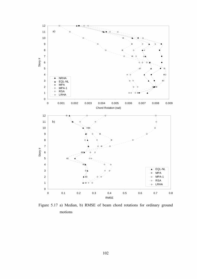
102
Figure 5.17 a) Median, b) RMSE of beam chord rotations for ordinary ground
motions
0
1
2
3
4
5
6
7
8
9
10
11
12
0 0.1 0.2 0.3 0.4 0.5 0.6 0.7 0.8
RMSE
Sto
ry #
EQL-NLMPAMPA-1RSALRHA
0
1
2
3
4
5
6
7
8
9
10
11
12
0 0.001 0.002 0.003 0.004 0.005 0.006 0.007 0.008 0.009
Chord Rotation (rad)
Sto
ry #
NRHAEQL-NLMPAMPA-1RSALRHA
a)
b)
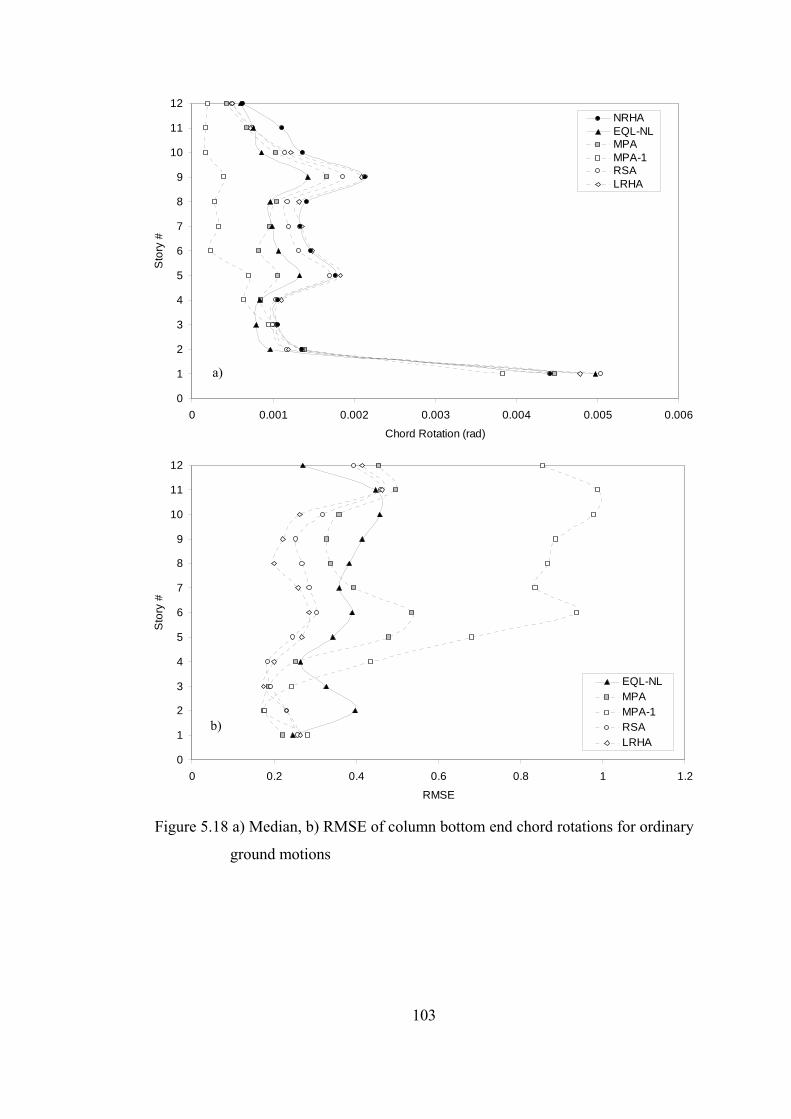
103
Figure 5.18 a) Median, b) RMSE of column bottom end chord rotations for ordinary
ground motions
0
1
2
3
4
5
6
7
8
9
10
11
12
0 0.2 0.4 0.6 0.8 1 1.2
RMSE
Sto
ry #
EQL-NLMPAMPA-1RSALRHA
0
1
2
3
4
5
6
7
8
9
10
11
12
0 0.001 0.002 0.003 0.004 0.005 0.006
Chord Rotation (rad)
Sto
ry #
NRHAEQL-NLMPAMPA-1RSALRHA
a)
b)
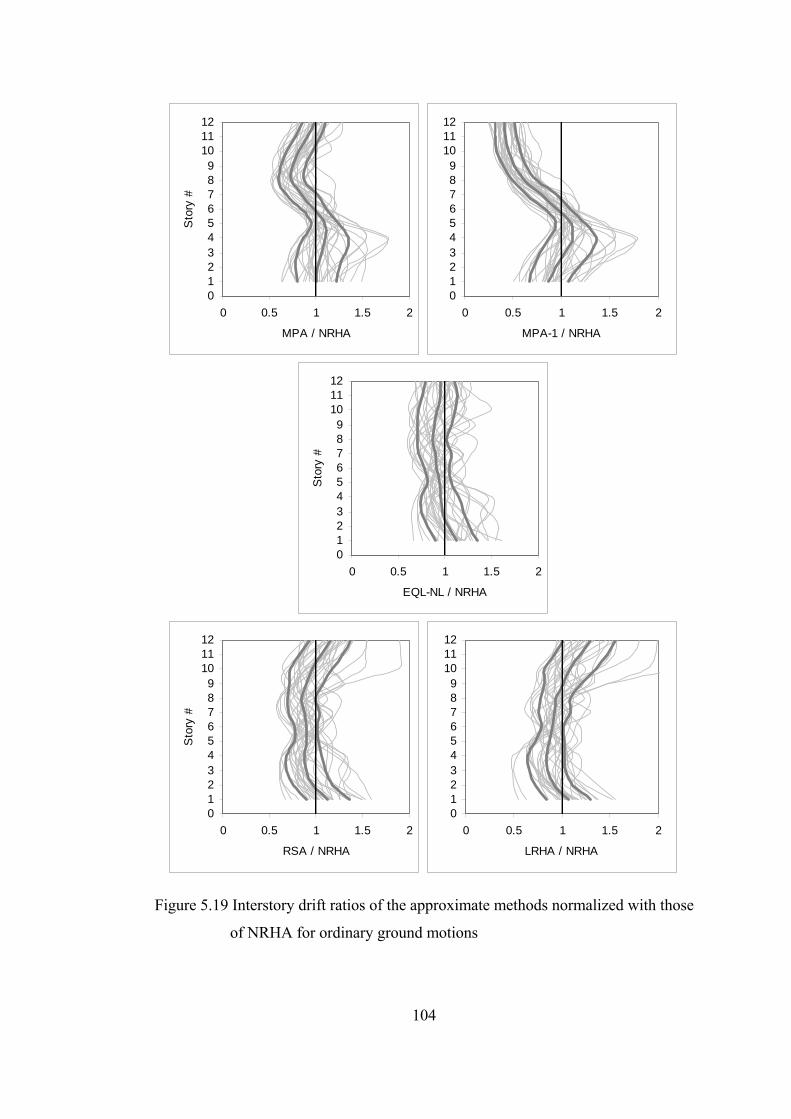
104
Figure 5.19 Interstory drift ratios of the approximate methods normalized with those
of NRHA for ordinary ground motions
0123456789
101112
0 0.5 1 1.5 2
EQL-NL / NRHA
Sto
ry #
0123456789
101112
0 0.5 1 1.5 2
MPA / NRHA
Sto
ry #
0123456789
101112
0 0.5 1 1.5 2
MPA-1 / NRHA
0123456789
101112
0 0.5 1 1.5 2
RSA / NRHA
Sto
ry #
0123456789
101112
0 0.5 1 1.5 2
LRHA / NRHA
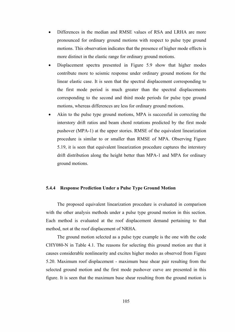
105
• Differences in the median and RMSE values of RSA and LRHA are more
pronounced for ordinary ground motions with respect to pulse type ground
motions. This observation indicates that the presence of higher mode effects is
more distinct in the elastic range for ordinary ground motions.
• Displacement spectra presented in Figure 5.9 show that higher modes
contribute more to seismic response under ordinary ground motions for the
linear elastic case. It is seen that the spectral displacement corresponding to
the first mode period is much greater than the spectral displacements
corresponding to the second and third mode periods for pulse type ground
motions, whereas differences are less for ordinary ground motions.
• Akin to the pulse type ground motions, MPA is successful in correcting the
interstory drift ratios and beam chord rotations predicted by the first mode
pushover (MPA-1) at the upper stories. RMSE of the equivalent linearization
procedure is similar to or smaller than RMSE of MPA. Observing Figure
5.19, it is seen that equivalent linearization procedure captures the interstory
drift distribution along the height better than MPA-1 and MPA for ordinary
ground motions.
5.4.4 Response Prediction Under a Pulse Type Ground Motion
The proposed equivalent linearization procedure is evaluated in comparison
with the other analysis methods under a pulse type ground motion in this section.
Each method is evaluated at the roof displacement demand pertaining to that
method, not at the roof displacement of NRHA.
The ground motion selected as a pulse type example is the one with the code
CHY080-N in Table 4.1. The reasons for selecting this ground motion are that it
causes considerable nonlinearity and excites higher modes as observed from Figure
5.20. Maximum roof displacement - maximum base shear pair resulting from the
selected ground motion and the first mode pushover curve are presented in this
figure. It is seen that the maximum base shear resulting from the ground motion is
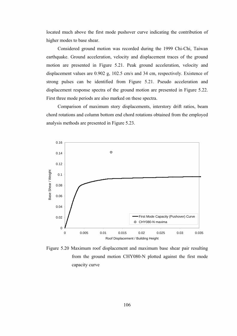
106
located much above the first mode pushover curve indicating the contribution of
higher modes to base shear.
Considered ground motion was recorded during the 1999 Chi-Chi, Taiwan
earthquake. Ground acceleration, velocity and displacement traces of the ground
motion are presented in Figure 5.21. Peak ground acceleration, velocity and
displacement values are 0.902 g, 102.5 cm/s and 34 cm, respectively. Existence of
strong pulses can be identified from Figure 5.21. Pseudo acceleration and
displacement response spectra of the ground motion are presented in Figure 5.22.
First three mode periods are also marked on these spectra.
Comparison of maximum story displacements, interstory drift ratios, beam
chord rotations and column bottom end chord rotations obtained from the employed
analysis methods are presented in Figure 5.23.
Figure 5.20 Maximum roof displacement and maximum base shear pair resulting
from the ground motion CHY080-N plotted against the first mode
capacity curve
0
0.02
0.04
0.06
0.08
0.1
0.12
0.14
0.16
0 0.005 0.01 0.015 0.02 0.025 0.03 0.035
Roof Displacement / Building Height
Bas
e S
hear
/ W
eigh
t
First Mode Capacity (Pushover) CurveCHY080-N maxima
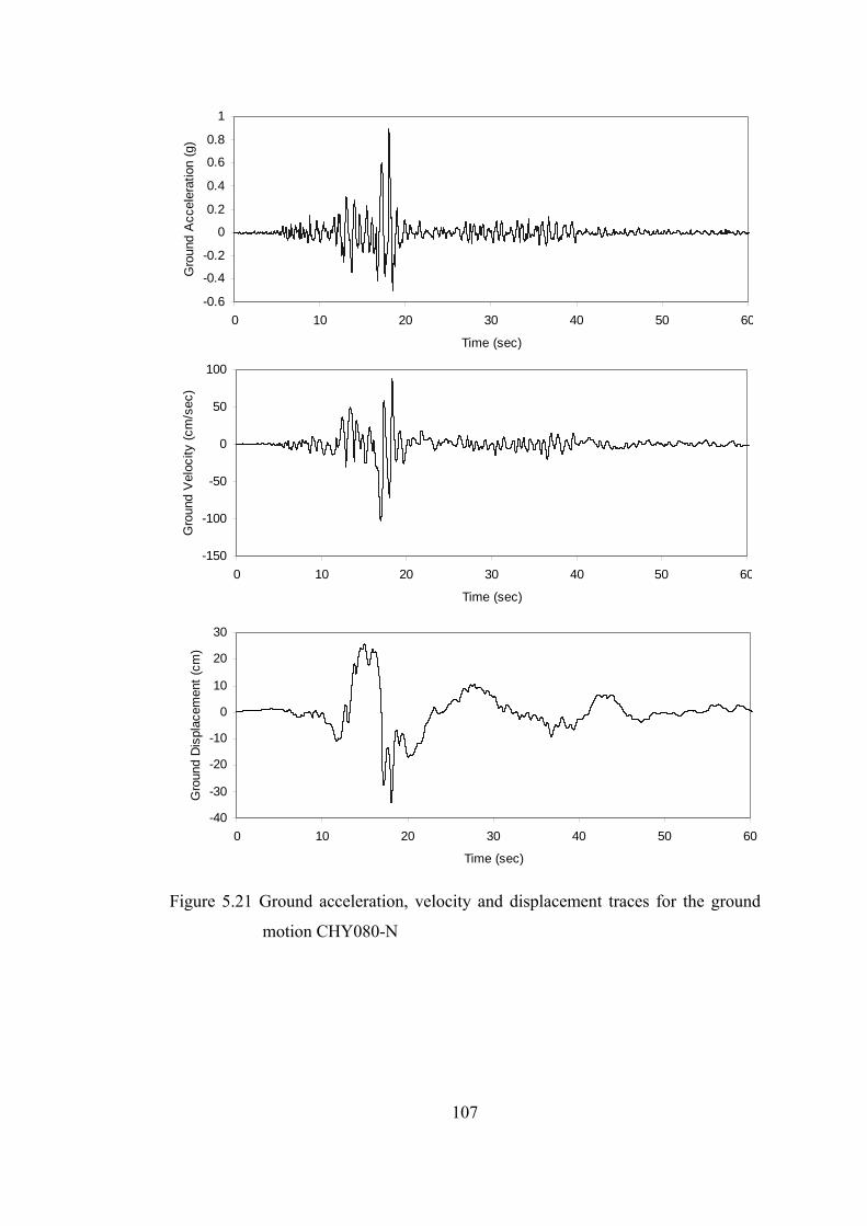
107
Figure 5.21 Ground acceleration, velocity and displacement traces for the ground
motion CHY080-N
-0.6
-0.4
-0.2
0
0.2
0.4
0.6
0.8
1
0 10 20 30 40 50 60
Time (sec)
Gro
und
Acc
eler
atio
n (g
)
-150
-100
-50
0
50
100
0 10 20 30 40 50 60
Time (sec)
Gro
und
Vel
ocity
(cm
/sec
)
-40
-30
-20
-10
0
10
20
30
0 10 20 30 40 50 60
Time (sec)
Gro
und
Dis
plac
emen
t (cm
)
108
Figure 5.22 5% damped pseudo acceleration and displacement response spectra for
the ground motion CHY080-N
0
0.1
0.2
0.3
0.4
0.5
0.6
0 0.5 1 1.5 2 2.5 3 3.5 4T (sec)
Sd
(m)
0
0.5
1
1.5
2
2.5
3
0 0.5 1 1.5 2 2.5 3 3.5 4T (sec)
PS
a (g
)
T1 T2 T3
T1 T2 T3
0.49
1.62
1.84
0.46
0.20
0.07
109
Figure 5.23 Comparison of maximum a) story displacements, b) interstory drift
ratios, c) beam chord rotations, d) column bottom end chord rotations
for the ground motion CHY080-N
0
1
2
3
4
5
6
7
8
9
10
11
12
0 0.2 0.4 0.6 0.8
Story Displacement (m)
Sto
ry #
NRHAEQL-NLEQL-EDRSALRHAMPAMPA-1
0
1
2
3
4
5
6
7
8
9
10
11
12
0 0.01 0.02 0.03
Interstory drift ratioS
tory
#
0
1
2
3
4
5
6
7
8
9
10
11
12
0 0.01 0.02 0.03
Chord Rotation (rad)
Sto
ry #
0
1
2
3
4
5
6
7
8
9
10
11
12
0 0.005 0.01 0.015 0.02
Chord Rotation (rad)
Sto
ry #
NRHAEQL-NLEQL-EDRSALRHAMPAMPA-1
a) b)
c) d)
110
Following observations can be made from Figure 5.23.
• Story displacements predicted by EQL-NL are close to those determined by
NRHA. EQL-NL is successful in improving the story displacements predicted
by RSA. Same observation is not true for EQL-ED. MPA and MPA-1 result
in sufficiently accurate story displacements for the presented ground motion.
• Distribution of interstory drift ratios and beam chord rotations along the
height are different for LRHA and NRHA. Presence of higher modes are more
pronounced for LRHA, but higher mode effects are also present in NRHA as
indicated from the base shear value in Figure 5.20 and the distribution of
interstory drift ratios along the height. EQL-NL results in sufficiently accurate
estimations of interstory drift ratios and beam chord rotations obtained by
NRHA.
• Although RSA and EQL-ED result in inaccurate roof displacement
estimations, they are successful in predicting some of the local response
parameters like the first story column bottom end chord rotations and beam
chord rotations at the intermediate story levels. In order to prevent a
misleading evaluation of the approximate methods in such cases, statistical
evaluation of the methods were conducted at the roof displacement demands
of NRHA as explained previously.
• There are differences between RSA and LRHA results, because higher mode
effects are considerable in the elastic range as can be noted from the
displacement response spectrum in Figure 5.22.
• MPA is satisfactory in estimating the beam chord rotations and interstory drift
ratios for the selected ground motion. It amplifies the predictions of MPA-1 at
the upper stories. MPA underestimates the column bottom end chord rotations
of the first story, which was previously noted for the median response under
the pulse type ground motion set.
111
5.4.5 Response Prediction Under an Ordinary Ground Motion
The ordinary ground motion for which the results are presented in this section
is the one with the code IZT090 in Table 4.2. First mode pushover curve and the
maximum roof displacement - maximum base shear pair resulting from the selected
ground motion are presented in Figure 5.24. It is seen that the maximum base shear
resulting from the ground motion is located much above the first mode capacity
curve indicating the presence of higher modes. This ground motion is selected for
presentation because higher mode effects are present both in LRHA and NRHA. In
addition, distribution of local responses along the height is considerably different in
LRHA and NRHA although the ground motion results in a moderate level of
inelasticity.
The selected ground motion is the 90 degree component of the ground motion
recorded in İzmit station during 1999 Kocaeli earthquake. Ground acceleration,
velocity and displacement traces of the ground motion are presented in Figure 5.25.
Peak ground acceleration, velocity and displacement values are 0.220 g, 29.8 cm/s
and 17.1 cm, respectively. Pseudo acceleration and displacement response spectra
of the ground motion are presented in Figure 5.26. First three mode periods are also
marked on these spectra.
Comparison of maximum story displacements, interstory drift ratios, beam
chord rotations and column bottom end chord rotations obtained from the employed
analysis methods are presented in Figure 5.27. Following observations are derived
from these figures.
• Story displacements predicted by EQL-NL are very close to those determined
by NRHA. EQL-NL is successful at improving the story displacements
predicted by RSA. As in the case of the pulse type ground motion example,
story displacements determined by EQL-ED and RSA are similar to each
other. MPA and MPA-1 overestimate the story displacements.
• Distribution of local responses along the height is considerably different for
LRHA and NRHA, although nonlinearity is not significant in the system.
Regarding this situation, EQL-NL is successful in predicting the interstory
112
drift ratios and beam chord rotations determined by NRHA. It improves the
predictions of RSA. EQL-NL overestimates the first story column bottom end
chord rotation, however since the value determined by NRHA is small,
overestimation does not introduce a significant problem.
• MPA improves the beam chord rotation and interstory drift ratio predictions
of MPA-1. Both MPA and MPA-1 overestimate the beam chord rotations and
interstory drift ratios at the lower stories.
Figure 5.24 Maximum roof displacement and maximum base shear pair resulting
from the ground motion IZT090 plotted against the first mode capacity
curve
0.00
0.02
0.04
0.06
0.08
0.10
0.12
0.000 0.005 0.010 0.015 0.020 0.025 0.030 0.035
Roof Displacement / Building Height
Bas
e S
hear
/ W
eigh
t
First Mode Capacity (Pushover) CurveIZT090 maxima
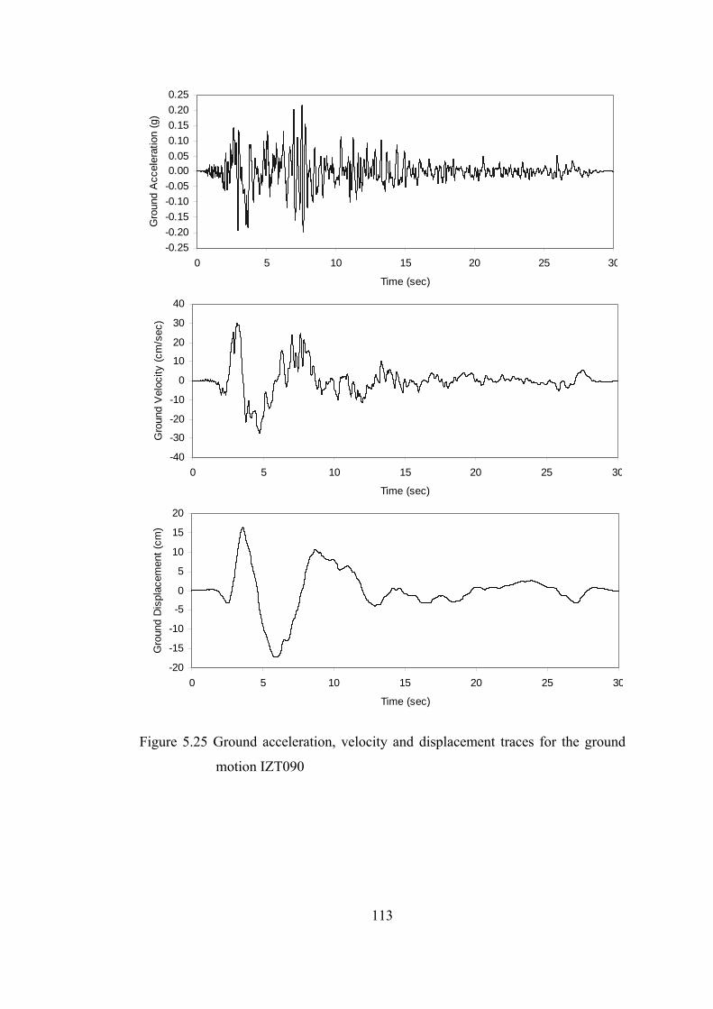
113
Figure 5.25 Ground acceleration, velocity and displacement traces for the ground
motion IZT090
-0.25-0.20-0.15-0.10-0.050.000.050.100.150.200.25
0 5 10 15 20 25 30
Time (sec)
Gro
und
Acc
eler
atio
n (g
)
-40
-30
-20
-10
0
10
20
30
40
0 5 10 15 20 25 30
Time (sec)
Gro
und
Vel
ocity
(cm
/sec
)
-20
-15
-10
-5
0
5
10
15
20
0 5 10 15 20 25 30
Time (sec)
Gro
und
Dis
plac
emen
t (cm
)
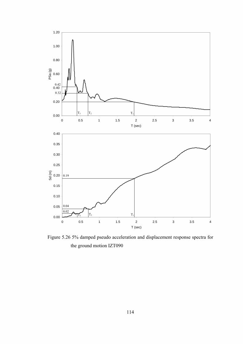
114
Figure 5.26 5% damped pseudo acceleration and displacement response spectra for
the ground motion IZT090
0.00
0.20
0.40
0.60
0.80
1.00
1.20
0 0.5 1 1.5 2 2.5 3 3.5 4T (sec)
PS
a (g
)
0.00
0.05
0.10
0.15
0.20
0.25
0.30
0.35
0.40
0 0.5 1 1.5 2 2.5 3 3.5 4T (sec)
Sd
(m)
T1 T2 T3
T1 T2 T3
0.42
0.32
0.19
0.04
0.02
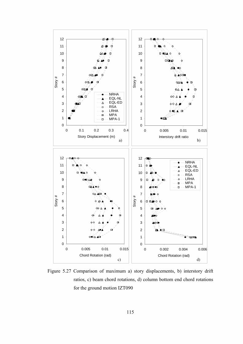
115
Figure 5.27 Comparison of maximum a) story displacements, b) interstory drift
ratios, c) beam chord rotations, d) column bottom end chord rotations
for the ground motion IZT090
0
1
2
3
4
5
6
7
8
9
10
11
12
0 0.1 0.2 0.3 0.4
Story Displacement (m)
Sto
ry #
NRHAEQL-NLEQL-EDRSALRHAMPAMPA-1
0
1
2
3
4
5
6
7
8
9
10
11
12
0 0.005 0.01 0.015
Interstory drift ratioS
tory
#
0
1
2
3
4
5
6
7
8
9
10
11
12
0 0.005 0.01 0.015
Chord Rotation (rad)
Sto
ry #
0
1
2
3
4
5
6
7
8
9
10
11
12
0 0.002 0.004 0.006
Chord Rotation (rad)
Sto
ry #
NRHAEQL-NLEQL-EDRSALRHAMPAMPA-1
a) b)
c) d)
116
CHAPTER 6
CASE STUDY II:
SIX STORY UNSYMMETRICAL-PLAN RC SPACE FRAME
6.1 Description of the Building
A six story reinforced concrete building frame is selected as the second case
study, for which the story plan and the 3D view are shown in Figure 6.1. The
building is designed according to the regulations of TS-500 (2000) and TEC (1998)
where capacity design requirements prevail. The building is assumed to be located
in seismic zone 1 with local site class Z3. Therefore an enhanced ductility level is
employed in design. Utilized concrete and steel grades are C25 and S420
respectively. Slab thickness for all floors is 14 cm and live load is taken as 2 kN/m2.
Dimensions of all beams are 30x55 cm2, whereas dimensions of all columns are
50x50 cm2. There is no basement; height of the ground story is 4 m, while the
height of other stories is 3 m. For the analysis of the building, eccentricity between
the center of stiffness (CS) and center of mass (CM) is increased to 15% of the plan
dimension in order to introduce asymmetry about the Y-axis as indicated in Figure
6.1. Labels of the Y-direction frames are also presented in this figure.
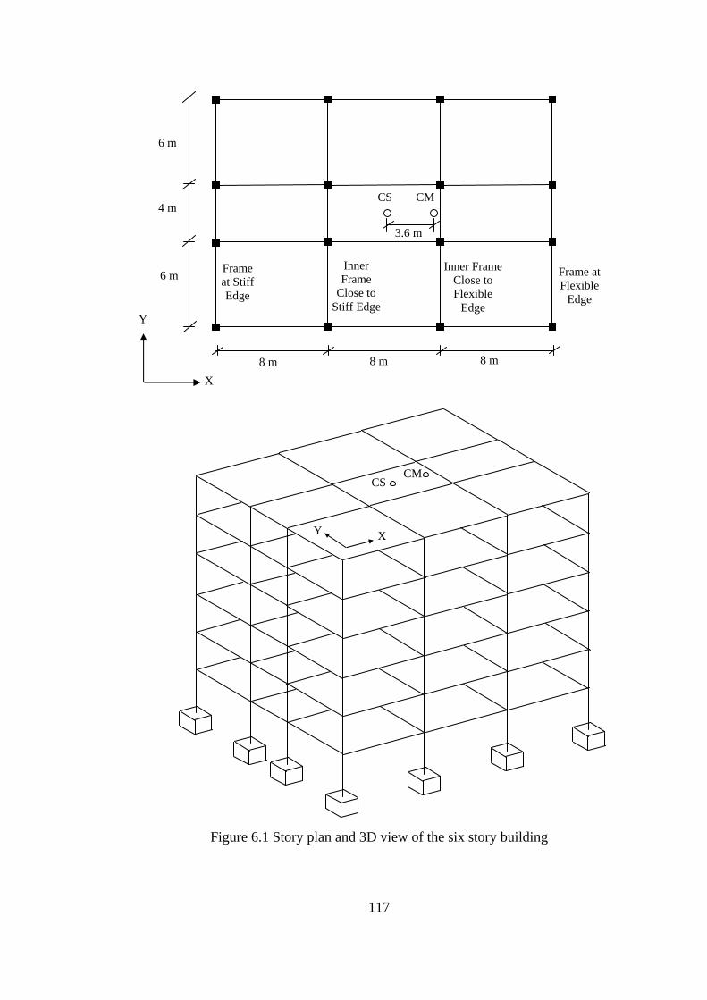
117
Figure 6.1 Story plan and 3D view of the six story building
6 m
4 m
6 m
8 m 8 m 8 m
X
Y
CS CM
3.6 m
X Y
CS CM
Frame at Stiff Edge
Inner Frame
Close to Stiff Edge
Inner Frame Close to Flexible
Edge
Frame at Flexible
Edge
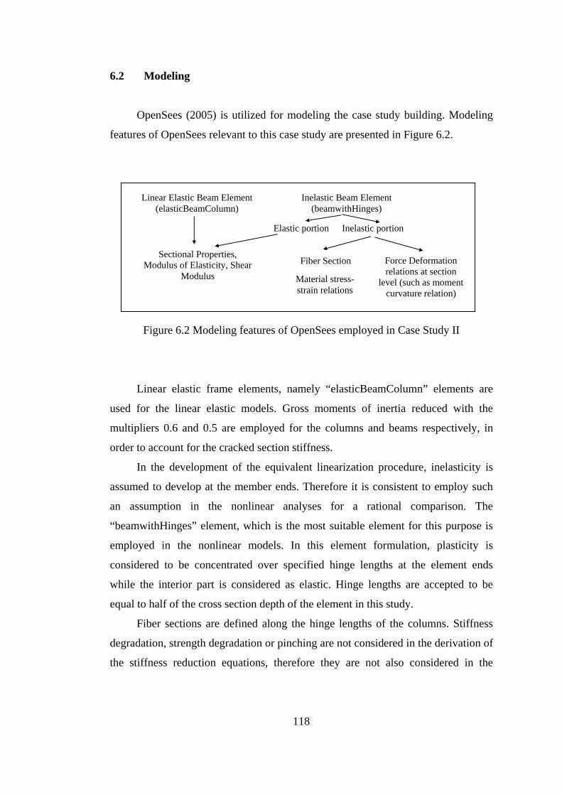
118
6.2 Modeling
OpenSees (2005) is utilized for modeling the case study building. Modeling
features of OpenSees relevant to this case study are presented in Figure 6.2.
Figure 6.2 Modeling features of OpenSees employed in Case Study II
Linear elastic frame elements, namely “elasticBeamColumn” elements are
used for the linear elastic models. Gross moments of inertia reduced with the
multipliers 0.6 and 0.5 are employed for the columns and beams respectively, in
order to account for the cracked section stiffness.
In the development of the equivalent linearization procedure, inelasticity is
assumed to develop at the member ends. Therefore it is consistent to employ such
an assumption in the nonlinear analyses for a rational comparison. The
“beamwithHinges” element, which is the most suitable element for this purpose is
employed in the nonlinear models. In this element formulation, plasticity is
considered to be concentrated over specified hinge lengths at the element ends
while the interior part is considered as elastic. Hinge lengths are accepted to be
equal to half of the cross section depth of the element in this study.
Fiber sections are defined along the hinge lengths of the columns. Stiffness
degradation, strength degradation or pinching are not considered in the derivation of
the stiffness reduction equations, therefore they are not also considered in the
Linear Elastic Beam Element(elasticBeamColumn)
Inelastic Beam Element (beamwithHinges)
Sectional Properties, Modulus of Elasticity, Shear
Modulus Fiber Section
Material stress-strain relations
Force Deformation relations at section
level (such as moment curvature relation)
Elastic portion Inelastic portion
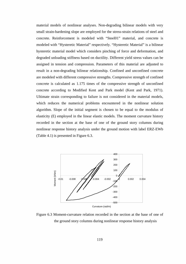
119
material models of nonlinear analyses. Non-degrading bilinear models with very
small strain-hardening slope are employed for the stress-strain relations of steel and
concrete. Reinforcement is modeled with “Steel01” material, and concrete is
modeled with “Hysteretic Material” respectively. “Hysteretic Material” is a bilinear
hysteretic material model which considers pinching of force and deformation, and
degraded unloading stiffness based on ductility. Different yield stress values can be
assigned in tension and compression. Parameters of this material are adjusted to
result in a non-degrading bilinear relationship. Confined and unconfined concrete
are modeled with different compressive strengths. Compressive strength of confined
concrete is calculated as 1.175 times of the compressive strength of unconfined
concrete according to Modified Kent and Park model (Kent and Park, 1971).
Ultimate strain corresponding to failure is not considered in the material models,
which reduces the numerical problems encountered in the nonlinear solution
algorithm. Slope of the initial segment is chosen to be equal to the modulus of
elasticity (E) employed in the linear elastic models. The moment curvature history
recorded in the section at the base of one of the ground story columns during
nonlinear response history analysis under the ground motion with label ERZ-EWb
(Table 4.1) is presented in Figure 6.3.
Figure 6.3 Moment-curvature relation recorded in the section at the base of one of
the ground story columns during nonlinear response history analysis
-500
-400
-300
-200
-100
0
100
200
300
400
-0.01 -0.008 -0.006 -0.004 -0.002 0 0.002 0.004
Curvature (rad/m)
Mom
ent (
kNm
)
120
Fiber sections are not utilized for the beams, because artificial axial forces
develop in the beams when fiber sections are employed despite the imposition of
diaphragm constraints. Diaphragm constraints impose the two ends of a beam,
located parallel to one of the transverse degrees of freedom of the mass center,
deform in equal amounts along the member axis. Since equal axial deformations are
imposed at the two ends, it is expected that the axial force in the beam is equal to
zero. However, this expectation does not hold in the presence of fiber sections and
axial forces develop, which in turn results in an increase in the moment capacities
of beams. Accordingly, a building designed for beam yielding may result in a
failure formation different than the intended if the design is based on a model
without fiber sections. Figure 6.4 shows the effect of utilizing fiber sections for
beam sections on the conventional pushover curve of the case study building. It can
be seen that fiber sections significantly increase the base shear capacity for the case
study building, which is a consequence of the increase in the moment capacities of
beams due to axial forces artificially developing in the fiber section model.
Existence of axial forces along the beam ends with floors acting as rigid diaphragms
should be investigated via experiments. In this study, it is accepted that axial force
does not exist along the beam axis in the presence of rigid diaphragms, and
accordingly fiber sections are not utilized for beams. Nondegrading bilinear
moment-curvature relations with very small strain hardening are utilized along the
hinge lengths of beams. Moment-curvature history recorded in a section at the end
of one of the first story beams during nonlinear response history analysis under the
ground motion with label ERZ-EWb (Table 4.1) is presented in Figure 6.5.
Since fiber sections are employed for the columns, cracking of concrete is
explicitly considered during the solution process. However bilinear moment-
curvature relations are utilized for the beams, for which it is not possible to consider
cracking during the solution process. Therefore, cracked section stiffness is
employed for the utilized moment-curvature relations. For this purpose, slope of the
initial line segment of the moment curvature relations is set to be 0.5EIgross, where E
is the modulus of elasticity and Igross is the gross moment of inertia. Moment of
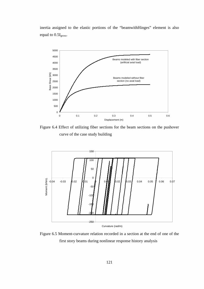
121
inertia assigned to the elastic portions of the “beamwithHinges” element is also
equal to 0.5Igross.
Figure 6.4 Effect of utilizing fiber sections for the beam sections on the pushover
curve of the case study building
Figure 6.5 Moment-curvature relation recorded in a section at the end of one of the
first story beams during nonlinear response history analysis
-250
-200
-150
-100
-50
0
50
100
150
-0.04 -0.03 -0.02 -0.01 0 0.01 0.02 0.03 0.04 0.05 0.06 0.07
Curvature (rad/m)
Mom
ent (
kNm
).
0
500
1000
1500
2000
2500
3000
3500
4000
4500
5000
0 0.1 0.2 0.3 0.4 0.5 0.6
Displacement (m)
Bas
e S
hear
(kN
)
Beams modeled with fiber section (artificial axial load)
Beams modeled without fiber section (no axial load)
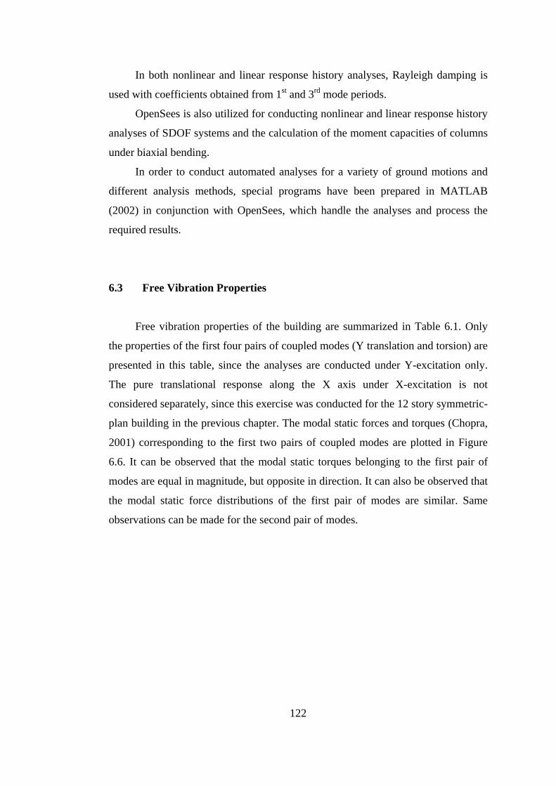
122
In both nonlinear and linear response history analyses, Rayleigh damping is
used with coefficients obtained from 1st and 3rd mode periods.
OpenSees is also utilized for conducting nonlinear and linear response history
analyses of SDOF systems and the calculation of the moment capacities of columns
under biaxial bending.
In order to conduct automated analyses for a variety of ground motions and
different analysis methods, special programs have been prepared in MATLAB
(2002) in conjunction with OpenSees, which handle the analyses and process the
required results.
6.3 Free Vibration Properties
Free vibration properties of the building are summarized in Table 6.1. Only
the properties of the first four pairs of coupled modes (Y translation and torsion) are
presented in this table, since the analyses are conducted under Y-excitation only.
The pure translational response along the X axis under X-excitation is not
considered separately, since this exercise was conducted for the 12 story symmetric-
plan building in the previous chapter. The modal static forces and torques (Chopra,
2001) corresponding to the first two pairs of coupled modes are plotted in Figure
6.6. It can be observed that the modal static torques belonging to the first pair of
modes are equal in magnitude, but opposite in direction. It can also be observed that
the modal static force distributions of the first pair of modes are similar. Same
observations can be made for the second pair of modes.
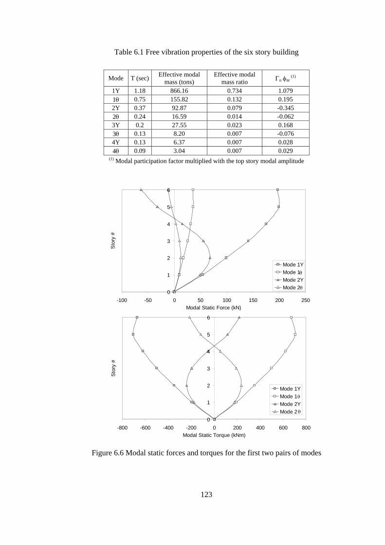
123
Table 6.1 Free vibration properties of the six story building
Mode T (sec) Effective modal
mass (tons) Effective modal
mass ratio Γn φnr (1)
1Y 1.18 866.16 0.734 1.079 1θ 0.75 155.82 0.132 0.195 2Y 0.37 92.87 0.079 -0.345 2θ 0.24 16.59 0.014 -0.062 3Y 0.2 27.55 0.023 0.168 3θ 0.13 8.20 0.007 -0.076 4Y 0.13 6.37 0.007 0.028 4θ 0.09 3.04 0.007 0.029
(1) Modal participation factor multiplied with the top story modal amplitude
Figure 6.6 Modal static forces and torques for the first two pairs of modes
0
1
2
3
4
5
6
-100 -50 0 50 100 150 200 250Modal Static Force (kN)
Sto
ry #
Mode 1YMode 1Mode 2YMode 2
θ
θ
0
1
2
3
4
5
6
-800 -600 -400 -200 0 200 400 600 800Modal Static Torque (kNm)
Stor
y #
Mode 1YMode 1Mode 2YMode 2
θ
θ
124
6.4 Presentation of Results
Maximum values of roof displacements, interstory drift ratios and chord
rotations are obtained for each Y direction frame under each ground motion
belonging to the two ground motion sets described in Chapter 4. The results from
nonlinear response history analysis (NRHA), modal pushover analysis (MPA),
conventional pushover analysis according to FEMA-356 (PO-FEMA), two variants
of the equivalent linearization procedure described in Chapter 3 (EQL-NL,
EQL-ED), linear elastic response spectrum analysis (RSA) and linear elastic
response history analysis (LRHA) are presented comparatively. A force distribution
proportional to the multiplication of the first mode shape and the mass matrix is
utilized as the lateral load pattern for PO-FEMA. Torsional components are not
considered and lateral forces are applied at the mass center of each story. However,
torsional forces are considered in each modal pushover of MPA as explained in
Chapter 2.
6.4.1 Roof (Top Story) Displacement Demands at the Center of Mass
Roof displacement demands at the center of mass calculated from the
approximate methods are plotted against those obtained from nonlinear response
history analyses (benchmark method) in Figures 6.7 and 6.8 for the 96 pulse type
and 66 ordinary ground motions, respectively. In these figures, displacements are in
meters. Calculated statistical parameters are summarized in Tables 6.2 and 6.3.
Investigation of Figures 6.7 and 6.8 and Tables 6.2 and 6.3 leads to similar
observations to those gathered from the roof displacement estimations of the twelve
story frame presented in the first case study.
LRHA and RSA produce erroneous estimations for both pulse type and
ordinary ground motions. Predictions of EQL-ED are close to those of RSA,
because same spectral displacements are employed in both of the methods,
moreover the mode shapes of the resulting equivalent linear systems are not much
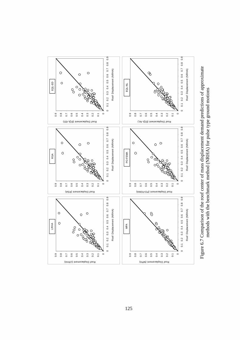
125
Figu
re 6
.7 C
ompa
rison
of t
he ro
of c
ente
r of m
ass d
ispl
acem
ent d
eman
d pr
edic
tions
of a
ppro
xim
ate
met
hods
with
the
benc
hmar
k m
etho
d (N
RH
A) f
or p
ulse
type
gro
und
mot
ions
0
0.1
0.2
0.3
0.4
0.5
0.6
0.7
0.8
0.9
00.
10.
20.
30.
40.
50.
60.
70.
80.
9
Roo
f D
ispl
acem
ent
(NR
HA
)
Roof Displacement (LRHA)
LRH
A
0
0.1
0.2
0.3
0.4
0.5
0.6
0.7
0.8
0.9
00.
10.
20.
30.
40.
50.
60.
70.
80.
9
Roo
f D
ispl
acem
ent
(NR
HA
)
Roof Displacement (RSA)
RS
A
0
0.1
0.2
0.3
0.4
0.5
0.6
0.7
0.8
0.9
00.
10.
20.
30.
40.
50.
60.
70.
80.
9
Roo
f D
ispl
acem
ent
(NR
HA
)
Roof Displacement (EQL-ED)
EQL-
ED
0
0.1
0.2
0.3
0.4
0.5
0.6
0.7
0.8
0.9
00.
10.
20.
30.
40.
50.
60.
70.
80.
9
Roo
f D
ispl
acem
ent
(NR
HA
)
Roof Displacement (MPA)
MPA
0
0.1
0.2
0.3
0.4
0.5
0.6
0.7
0.8
0.9
00.
10.
20.
30.
40.
50.
60.
70.
80.
9
Roo
f D
ispl
acem
ent
(NR
HA
)
Roof Displacement (PO-FEMA)
PO
-FE
MA
0
0.1
0.2
0.3
0.4
0.5
0.6
0.7
0.8
0.9
00.
10.
20.
30.
40.
50.
60.
70.
80.
9
Roo
f D
ispl
acem
ent
(NR
HA
)
Roof Displacement (EQL-NL)
EQ
L-N
L
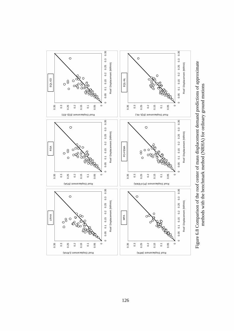
126
Figu
re 6
.8 C
ompa
rison
of t
he ro
of c
ente
r of m
ass d
ispl
acem
ent d
eman
d pr
edic
tions
of a
ppro
xim
ate
met
hods
with
the
benc
hmar
k m
etho
d (N
RH
A) f
or o
rdin
ary
grou
nd m
otio
ns
0
0.050.1
0.150.2
0.250.3
0.35
00.
050.
10.
150.
20.
250.
30.
35
Roo
f D
ispl
acem
ent (
NR
HA
)
Roof Displacement (LRHA)
LRH
A
0
0.050.1
0.150.2
0.250.3
0.35
00.
050.
10.
150.
20.
250.
30.
35
Roo
f D
ispl
acem
ent (
NR
HA
)
Roof Displacement (RSA)
RS
A
0
0.050.1
0.150.2
0.250.3
0.35
00.
050.
10.
150.
20.
250.
30.
35
Roo
f D
ispl
acem
ent (
NR
HA
)
Roof Displacement (EQL-ED)
EQ
L-E
D
0
0.050.1
0.150.2
0.250.3
0.35
00.
050.
10.
150.
20.
250.
30.
35
Roo
f D
ispl
acem
ent (
NR
HA
)
Roof Displacement (MPA)
MP
A
0
0.050.1
0.150.2
0.250.3
0.35
00.
050.
10.
150.
20.
250.
30.
35
Roo
f D
ispl
acem
ent (
NR
HA
)
Roof Displacement (PO-FEMA)
PO
-FE
MA
0
0.050.1
0.150.2
0.250.3
0.35
00.
050.
10.
150.
20.
250.
30.
35
Roo
f D
ispl
acem
ent (
NR
HA
)
Roof Displacement (EQL-NL)
EQL-
NL
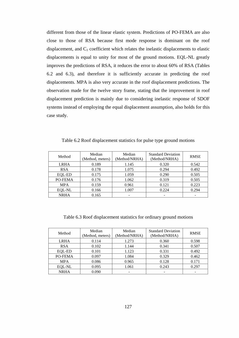
127
different from those of the linear elastic system. Predictions of PO-FEMA are also
close to those of RSA because first mode response is dominant on the roof
displacement, and C1 coefficient which relates the inelastic displacements to elastic
displacements is equal to unity for most of the ground motions. EQL-NL greatly
improves the predictions of RSA, it reduces the error to about 60% of RSA (Tables
6.2 and 6.3), and therefore it is sufficiently accurate in predicting the roof
displacements. MPA is also very accurate in the roof displacement predictions. The
observation made for the twelve story frame, stating that the improvement in roof
displacement prediction is mainly due to considering inelastic response of SDOF
systems instead of employing the equal displacement assumption, also holds for this
case study.
Table 6.2 Roof displacement statistics for pulse type ground motions
Method Median
(Method, meters)Median
(Method/NRHA) Standard Deviation (Method/NRHA) RMSE
LRHA 0.189 1.145 0.320 0.542 RSA 0.178 1.075 0.294 0.492
EQL-ED 0.175 1.059 0.290 0.505 PO-FEMA 0.176 1.062 0.319 0.505
MPA 0.159 0.961 0.121 0.223 EQL-NL 0.166 1.007 0.224 0.294 NRHA 0.165 - - -
Table 6.3 Roof displacement statistics for ordinary ground motions
Method Median
(Method, meters)Median
(Method/NRHA) Standard Deviation (Method/NRHA) RMSE
LRHA 0.114 1.273 0.360 0.598 RSA 0.102 1.144 0.341 0.507
EQL-ED 0.101 1.123 0.331 0.492 PO-FEMA 0.097 1.084 0.329 0.462
MPA 0.086 0.965 0.128 0.171 EQL-NL 0.095 1.061 0.243 0.297 NRHA 0.090 - - -
128
Roof displacement demands under ordinary ground motions are smaller than
the roof displacement demands under pulse type ground motions. However, RMSE
of RSA and LRHA are similarly large for pulse type and ordinary ground motions,
which indicates that the nonlinear roof displacements deviate from the linear ones at
small to moderate levels of nonlinearity.
6.4.2 Local Response Parameters
Comparison of roof displacements (for frames), interstory drift ratios and
beam chord rotations obtained from the previously mentioned analysis methods are
presented in this section. Column chord rotations are not presented, because only
the bottom ends of the first story columns exceed yield rotations. According to the
definition of chord rotation stated in Chapter 3, bottom end chord rotation of a first
story column is equal to the interstory drift ratio of the first story. Since the
interstory drift ratios are presented, there remains no need for the presentation of
column chord rotations.
For the comparison of local response parameters, ground motions producing
NRHA center of mass roof displacements between 0.150 m (0.79 % roof drift) and
0.550 m (2.90 % roof drift) are taken into consideration. Lower bound corresponds
to the onset of inelasticity. An upper bound is also set because P-Δ effects are not
considered and ultimate curvature values are not utilized in the moment curvature
relations. The number of pulse type and ordinary ground motions remaining in
between these bounds are 51 and 11, respectively. Roof displacement demands of
these ground motions normalized by the building height are marked on the first
mode pushover curve of the building in Figure 6.9. Base shear capacity prediction
of the equivalent linearization procedure is also shown with a horizontal line. It is
noted that base shear capacity obtained from the equivalent linearization procedure
is quite close to the one obtained from pushover analysis.
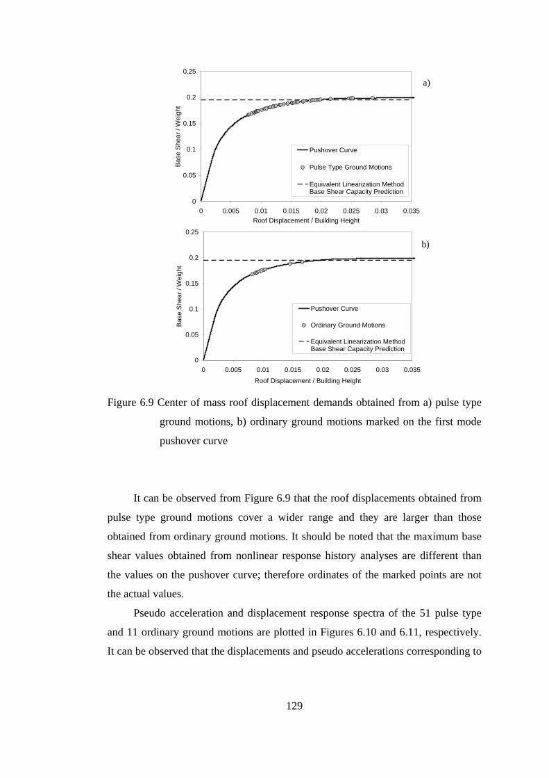
129
Figure 6.9 Center of mass roof displacement demands obtained from a) pulse type
ground motions, b) ordinary ground motions marked on the first mode
pushover curve
It can be observed from Figure 6.9 that the roof displacements obtained from
pulse type ground motions cover a wider range and they are larger than those
obtained from ordinary ground motions. It should be noted that the maximum base
shear values obtained from nonlinear response history analyses are different than
the values on the pushover curve; therefore ordinates of the marked points are not
the actual values.
Pseudo acceleration and displacement response spectra of the 51 pulse type
and 11 ordinary ground motions are plotted in Figures 6.10 and 6.11, respectively.
It can be observed that the displacements and pseudo accelerations corresponding to
0
0.05
0.1
0.15
0.2
0.25
0 0.005 0.01 0.015 0.02 0.025 0.03 0.035Roof Displacement / Building Height
Bas
e S
hear
/ W
eigh
t
Pushover Curve
Pulse Type Ground Motions
Equivalent Linearization MethodBase Shear Capacity Prediction
a)
b)
0
0.05
0.1
0.15
0.2
0.25
0 0.005 0.01 0.015 0.02 0.025 0.03 0.035Roof Displacement / Building Height
Bas
e S
hear
/ W
eigh
t
Pushover Curve
Ordinary Ground Motions
Equivalent Linearization MethodBase Shear Capacity Prediction
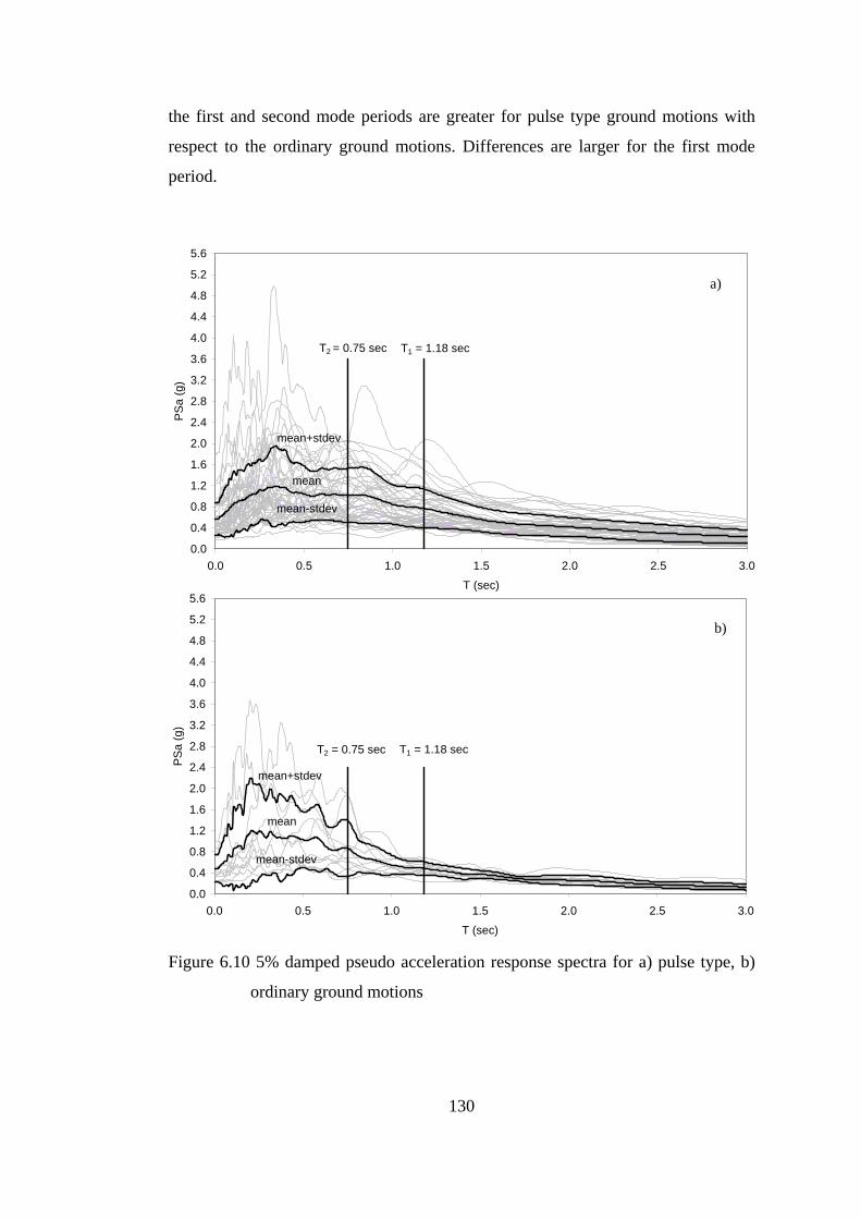
130
the first and second mode periods are greater for pulse type ground motions with
respect to the ordinary ground motions. Differences are larger for the first mode
period.
Figure 6.10 5% damped pseudo acceleration response spectra for a) pulse type, b)
ordinary ground motions
0.0
0.4
0.8
1.2
1.6
2.0
2.4
2.8
3.2
3.6
4.0
4.4
4.8
5.2
5.6
0.0 0.5 1.0 1.5 2.0 2.5 3.0
T (sec)
PSa
(g)
mean
mean+stdev
mean-stdev
T1 = 1.18 secT2 = 0.75 sec
0.0
0.4
0.8
1.2
1.6
2.0
2.4
2.8
3.2
3.6
4.0
4.4
4.8
5.2
5.6
0.0 0.5 1.0 1.5 2.0 2.5 3.0
T (sec)
PSa
(g)
mean
mean+stdev
mean-stdev
T1 = 1.18 secT2 = 0.75 sec
a)
b)
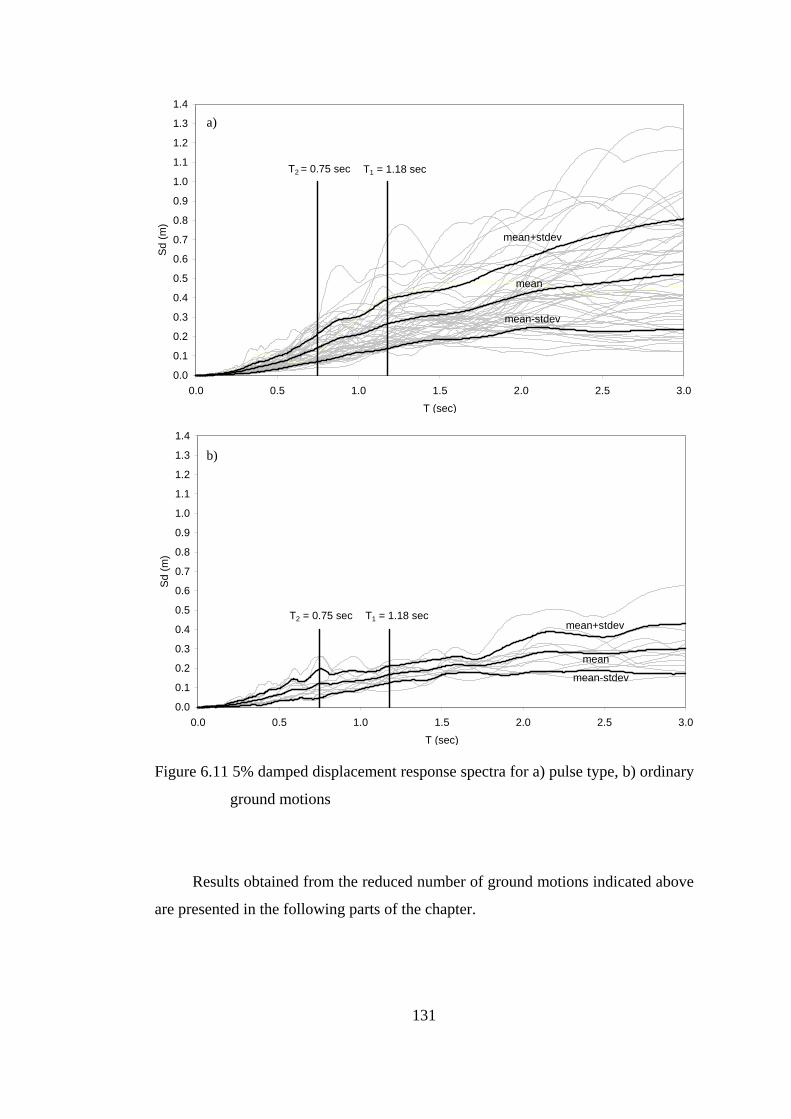
131
Figure 6.11 5% damped displacement response spectra for a) pulse type, b) ordinary
ground motions
Results obtained from the reduced number of ground motions indicated above
are presented in the following parts of the chapter.
0.0
0.1
0.2
0.3
0.4
0.5
0.6
0.7
0.8
0.9
1.0
1.1
1.2
1.3
1.4
0.0 0.5 1.0 1.5 2.0 2.5 3.0T (sec)
Sd
(m)
mean
mean+stdev
mean-stdev
T1 = 1.18 secT2 = 0.75 sec
0.0
0.1
0.2
0.3
0.4
0.5
0.6
0.7
0.8
0.9
1.0
1.1
1.2
1.3
1.4
0.0 0.5 1.0 1.5 2.0 2.5 3.0T (sec)
Sd
(m)
mean
mean+stdev
mean-stdev
T1 = 1.18 secT2 = 0.75 sec
a)
b)
132
In order to eliminate the effect of errors due to the differences in the
maximum roof displacements at the center of mass, response predictions of the
approximate methods are evaluated at roof displacements equal to the maximum
roof displacement obtained from NRHA. Such a modification is necessary, because
especially the edge frame responses are affected by the magnitude of the lateral
displacement at the center of mass and the amount of torsion emanating from the
rotation of the center of mass, as presented in the following section. Equating the
roof displacements, it is intended to evaluate the approximate methods’ accuracy for
considering torsion and the inelasticity distribution along the height. Local response
parameters determined by EQL-ED are not presented further because they are close
to those of EQL-NL at equal roof displacements. In the following part of the
chapter, pushover analysis is abbreviated as “PO” instead of “PO-FEMA” since it is
evaluated at the roof displacement of NRHA. It should be reminded again that only
lateral forces at the center of mass are employed and torques are not considered in
the force distribution of PO.
6.4.2.1 Torsional Effects Observed in Nonlinear Response History Analyses
In order to investigate the amount of torsion arising from asymmetry in plan,
median interstory drift ratios obtained from the benchmark method (nonlinear
response history analysis) at each frame are plotted in Figure 6.12. Labeling of the
frames was presented in Figure 6.1. It can be observed that considerable torsion
occurs both for pulse type and ordinary ground motions. It can also be seen that
median interstory drift ratios of the pulse type ground motions are greater than those
of the ordinary ground motions, similar to the case of roof displacements.
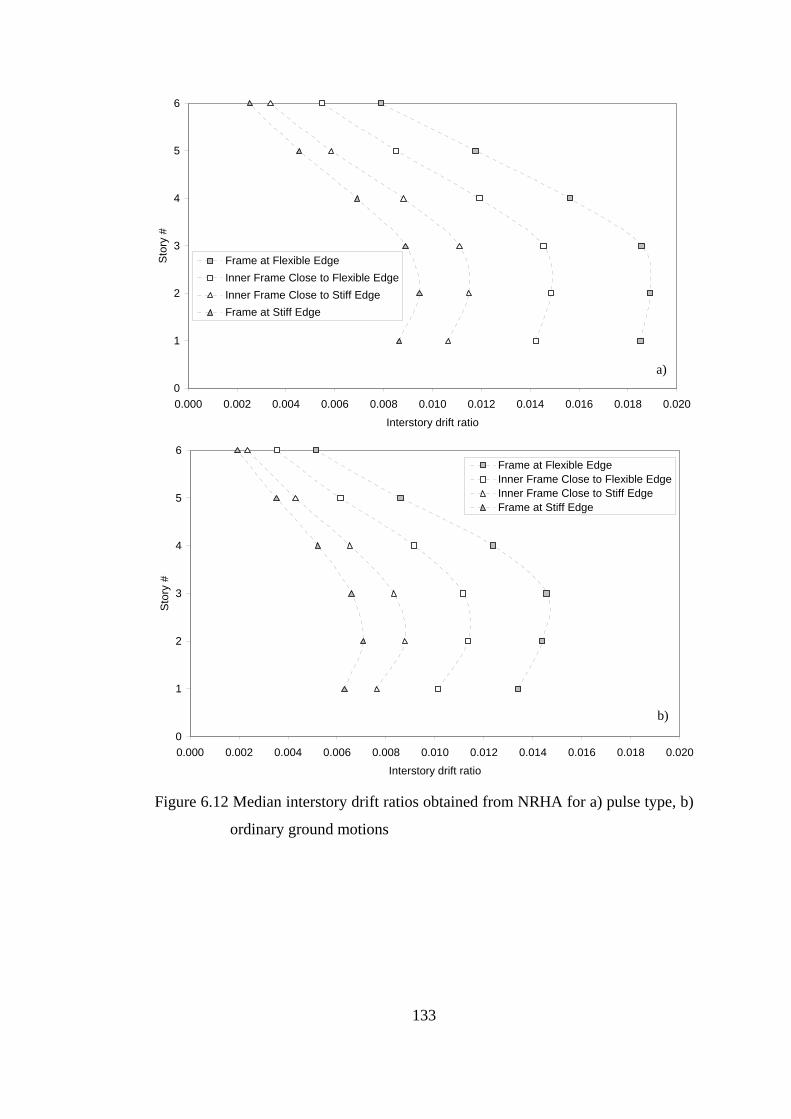
133
Figure 6.12 Median interstory drift ratios obtained from NRHA for a) pulse type, b)
ordinary ground motions
0
1
2
3
4
5
6
0.000 0.002 0.004 0.006 0.008 0.010 0.012 0.014 0.016 0.018 0.020
Interstory drift ratio
Sto
ry #
Frame at Flexible EdgeInner Frame Close to Flexible EdgeInner Frame Close to Stiff EdgeFrame at Stiff Edge
0
1
2
3
4
5
6
0.000 0.002 0.004 0.006 0.008 0.010 0.012 0.014 0.016 0.018 0.020
Interstory drift ratio
Sto
ry #
Frame at Flexible EdgeInner Frame Close to Flexible EdgeInner Frame Close to Stiff EdgeFrame at Stiff Edge
a)
b)
134
6.4.2.2 Roof Displacements of the Frames
Median and RMSE of roof displacements of the four individual frames are
presented in the form of bar charts in Figures 6.13 and 6.14 for pulse type and
ordinary ground motions respectively. Following observations can be made from
the investigation of these figures.
• Median roof displacements of the inner frame close to the flexible edge
predicted by the approximate methods are very similar to those determined by
NRHA for both types of ground motions. In addition, RMSE of the
approximate methods are quite close to zero for this frame since center of
mass is located close to this frame (Figure 6.1). Considering that the
approximate methods are evaluated at the center of mass roof displacements
determined by NRHA, it is evident that the roof displacements predicted by
the approximate methods are very close to those of NRHA at the inner frame
close to the flexible edge.
• EQL-NL is sufficiently accurate in predicting the roof displacements of
frames for both pulse type and ordinary ground motions. It results in
predictions close to NRHA at the medial level. It leads to the smallest RMSE
among the considered approximate methods for all the frames under pulse
type ground motions and for all the frames, except the stiff edge frame, under
ordinary ground motions. It greatly reduces RMSE of RSA at the stiff edge
frame under ordinary ground motions.
• There are considerable differences between RMSE of RSA and LRHA
especially at the edge frames under ordinary ground motions, indicating that
these two methods may lead to significantly different responses.
• Main reason of the difference between the response predictions of RSA and
LRHA is the torsional components of the modal forces. In Figure 6.6, it can
be observed that the modal static torques corresponding to the first pair of
modes are equal in magnitude but opposite in direction. The situation is
similar for the second pair of modes. Effect of opposite directions is lost in
135
RSA since the maximum responses in each mode are combined with a
combination rule. For this case study building, CQC is employed as the
combination rule in which the sign of the responses are taken into
consideration. However, the cross correlation coefficients come out to be
small since the natural periods are not so close. Therefore, responses from the
different modes are additive in RSA. In the case that the maximum elastic
SDOF accelerations in the coupling modes possess the same signs, differences
between the response predictions of RSA and LRHA deviate from each other.
Because, in this case, effect of the torques are counteracting in LRHA and
they are additive in RSA.
• PO slightly underestimates the roof displacements at the edge frames for both
types of ground motions. It results in median values similar to those of NRHA
at the inner frames.
• MPA underestimates the response at the stiff edge and overestimates the
response at the flexible edge because of overestimation of torsion. Cause of
this overestimation is the torsional component of the first modal force. First
mode response is generally dominant in MPA, since the center of mass roof
displacement demands of the other modes are small. In the higher modes,
base shear capacities are higher, periods are smaller and modal participation
factors multiplied with the top story modal amplitudes are smaller than those
corresponding to the first mode. Therefore roof displacement demands of
these modes are generally quite small when compared to that of the first
mode. In the first mode, the torsional component of the first mode vector
decreases the equivalent lateral forces acting at the stiff edge frame and
increases the equivalent lateral forces acting at the flexible edge frame.
Equivalent lateral static first mode forces for the linear elastic system acting at
the stiff and flexible edge frames with and without the torques at the center of
mass are presented in Figure 6.15. Forces corresponding to the case with
torques at the center of mass belong to the MPA first mode distribution and
forces corresponding to the case without torques at the center of mass belong
to PO force distribution. During NRHA, if the signs of the response

136
accelerations of the coupled modes are the same, torques of the coupled
modes counteract and only lateral forces remain. In such cases, MPA
underestimates the response at the stiff edge and overestimates the response at
the flexible edge, whereas PO does not result in such an overestimation or
underestimation because of the torsion effect since only the lateral forces are
considered in the force distribution of PO.
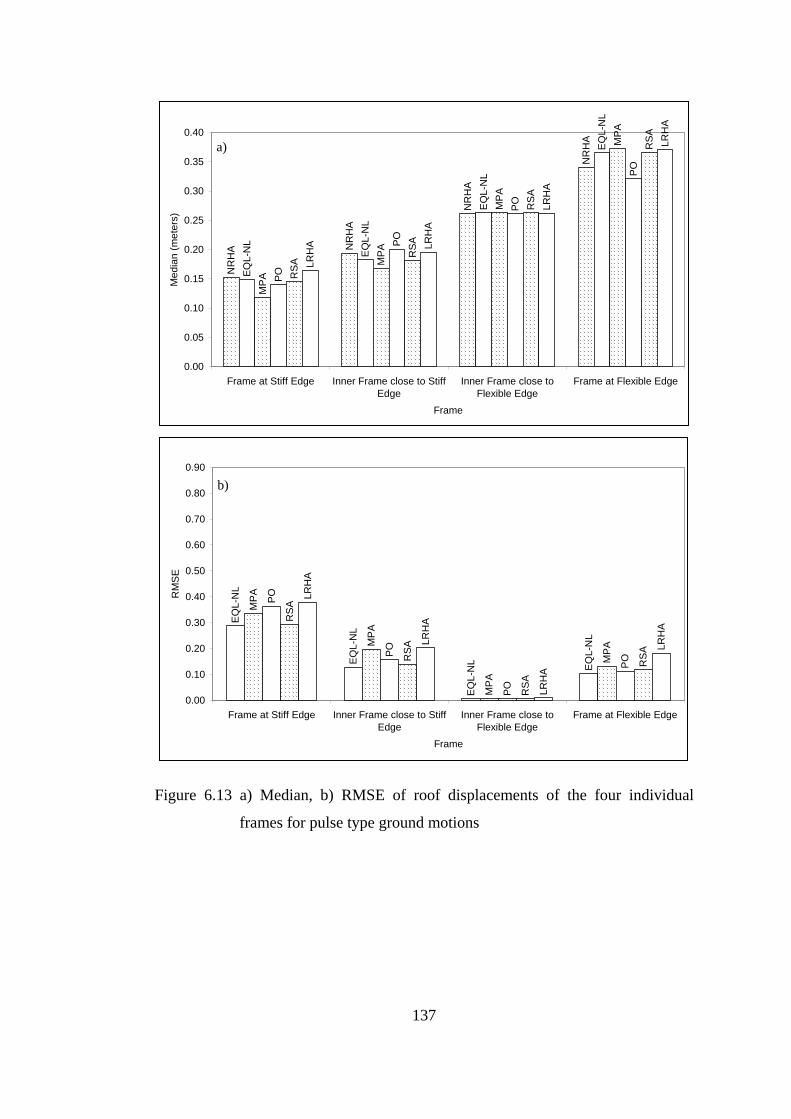
137
Figure 6.13 a) Median, b) RMSE of roof displacements of the four individual
frames for pulse type ground motions
NR
HA N
RH
A
NR
HA
NR
HA
EQL-
NL
EQ
L-N
L
EQ
L-N
L
EQL-
NL
MPA
MP
A
MPA
MPA
PO
PO
PO
PO
RSA
RSA
RS
A
RS
A
LRH
A LRH
A
LRH
A
LRH
A
0.00
0.05
0.10
0.15
0.20
0.25
0.30
0.35
0.40
Frame at Stiff Edge Inner Frame close to StiffEdge
Inner Frame close toFlexible Edge
Frame at Flexible Edge
Frame
Med
ian
(met
ers)
EQ
L-N
L
EQL-
NL
EQL-
NL EQ
L-N
L
MPA
MP
A
MPA
MPA
PO
PO
PO
PO
RS
A
RSA
RSA
RSA
LRH
A
LRH
A
LRH
A
LRH
A
0.00
0.10
0.20
0.30
0.40
0.50
0.60
0.70
0.80
0.90
Frame at Stiff Edge Inner Frame close to StiffEdge
Inner Frame close toFlexible Edge
Frame at Flexible Edge
Frame
RM
SE
a)
b)
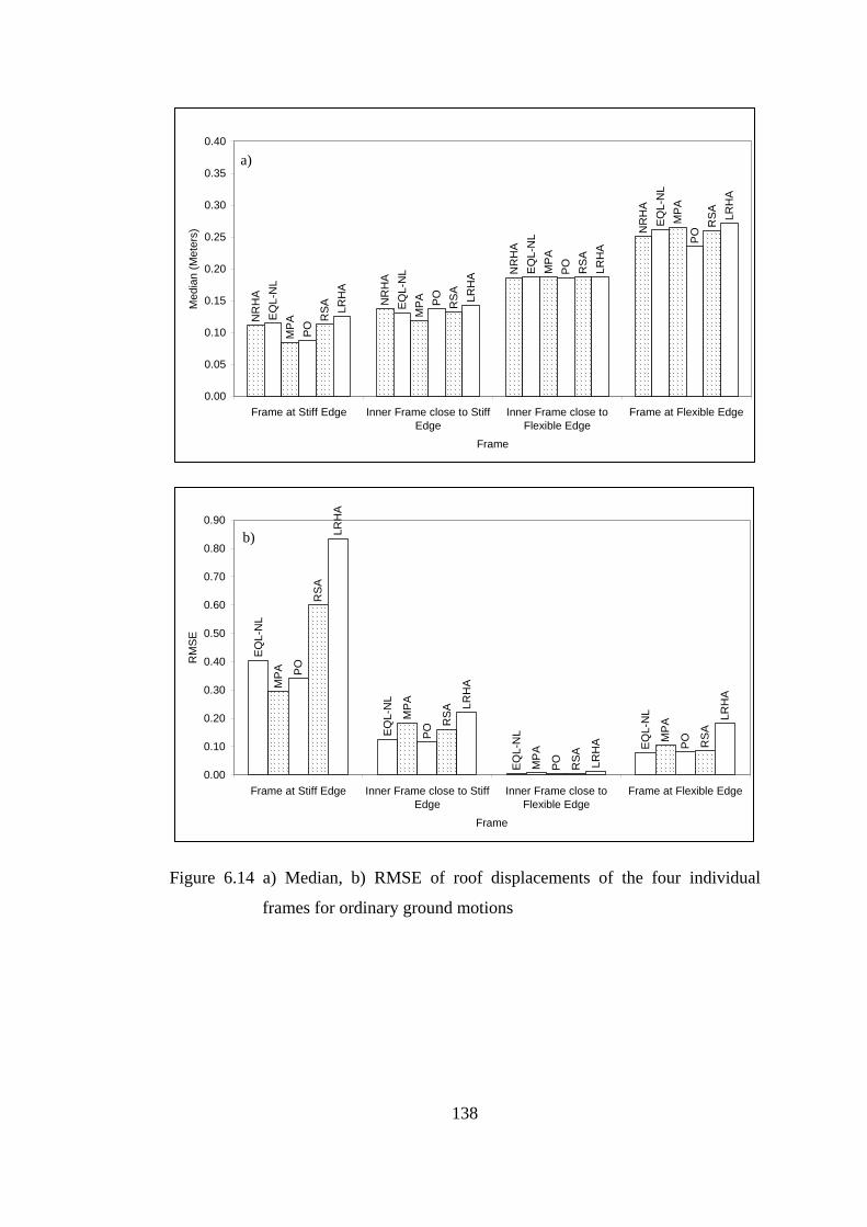
138
Figure 6.14 a) Median, b) RMSE of roof displacements of the four individual
frames for ordinary ground motions
NR
HA
NR
HA N
RH
A
NR
HA
EQL-
NL
EQL-
NL EQ
L-N
L
EQL-
NL
MPA
MPA
MPA
MPA
PO
PO
PO
PO
RSA R
SA
RS
A
RSA
LRH
A
LRH
A LRH
A
LRH
A
0.00
0.05
0.10
0.15
0.20
0.25
0.30
0.35
0.40
Frame at Stiff Edge Inner Frame close to StiffEdge
Inner Frame close toFlexible Edge
Frame at Flexible Edge
Frame
Med
ian
(Met
ers)
a)
EQL-
NL
EQL-
NL
EQL-
NL
EQL-
NL
MPA
MPA
MPA
MPA
PO
PO
PO
PO
RSA
RSA
RSA
RSA
LRH
A
LRH
A
LRH
A
LRH
A
0.00
0.10
0.20
0.30
0.40
0.50
0.60
0.70
0.80
0.90
Frame at Stiff Edge Inner Frame close to StiffEdge
Inner Frame close toFlexible Edge
Frame at Flexible Edge
Frame
RM
SE
b)
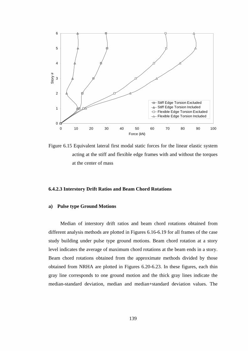
139
Figure 6.15 Equivalent lateral first modal static forces for the linear elastic system
acting at the stiff and flexible edge frames with and without the torques
at the center of mass
6.4.2.3 Interstory Drift Ratios and Beam Chord Rotations
a) Pulse type Ground Motions
Median of interstory drift ratios and beam chord rotations obtained from
different analysis methods are plotted in Figures 6.16-6.19 for all frames of the case
study building under pulse type ground motions. Beam chord rotation at a story
level indicates the average of maximum chord rotations at the beam ends in a story.
Beam chord rotations obtained from the approximate methods divided by those
obtained from NRHA are plotted in Figures 6.20-6.23. In these figures, each thin
gray line corresponds to one ground motion and the thick gray lines indicate the
median-standard deviation, median and median+standard deviation values. The
0
1
2
3
4
5
6
0 10 20 30 40 50 60 70 80 90 100Force (kN)
Sto
ry #
Stiff Edge Torsion ExcludedStiff Edge Torsion IncludedFlexible Edge Torsion ExcludedFlexible Edge Torsion Included
140
black line belongs to the ground motion selected for presentation in the following
sections. Following observations can be deduced from Figures 6.16-6.23.
• Equivalent linearization procedure is successful in improving the median
predictions of RSA for all frames, with reference to NRHA. Improvement in
the beam chord rotation estimations is more pronounced than the
improvement in interstory drift ratios. There is considerable improvement in
the beam chord rotations at the flexible edge frame and at the inner frame
close to the flexible edge where inelasticity is larger.
• Observing the dispersion in the beam chord rotations in Figures 6.20-6.23, it
can be stated that the equivalent linearization procedure reduces the scatter
present in RSA or results in similar amounts of scatter with RSA. For both
situations, errors are reduced since the equivalent linearization procedure
improves the median predictions.
• Generally, RSA and LRHA underestimate the beam chord rotations and
interstory drift ratios with large amounts of dispersion. LRHA overestimates
the top two story responses. As can be seen from Figures 6.20-6.23, there are
substantial differences between the beam chord rotation predictions of RSA
and LRHA because of the differences in the consideration of torsional
components of modal forces as explained previously.
• PO seems to be very successful in the median predictions except in the top
two stories for all frames. However, concerning the dispersion, it is seen that
there is large amount of scatter at the stiff edge frame and the inner frame
close to the stiff edge. Scatter is small at the lower stories of the flexible edge
frame and the inner frame close to the flexible edge. Therefore, PO can be
regarded as satisfactory in estimating the responses at the flexible edge except
the top stories. It underestimates the responses at the top two stories of all
frames. EQL-NL is more successful at the top two stories with respect to PO.
EQL-NL also underestimates the response at the top two stories; however the
amount of underestimation is smaller. Dispersion in the normalized beam
chord rotations of EQL-NL is much smaller than that of PO at the stiff edge
141
(Figures 6.20 and 6.21). Errors of EQL-NL and PO are similar at the flexible
edge frame, PO being more accurate at the first story and EQL-NL being
more accurate at the top two stories. Overall, it can be stated that response
predictions of the equivalent linearization procedure are as accurate as the
response predictions of the conventional pushover analysis, they are more
accurate at the top stories at which conventional pushover possesses a
drawback in considering the higher mode effects.
• MPA underestimates the response at the stiff edge frame and overestimates
the response at the lower three stories of the flexible edge frame because of
the overestimated torsion as explained in Section 6.4.2.2. Underestimations at
the stiff edge frame are clearly observed in Figure 6.20. In this figure, it is
seen that MPA underestimates the beam chord rotations at all of the stories
under nearly all of the ground motions. It overestimates the beam chord
rotations at the lower two stories of the flexible edge frame under nearly all of
the ground motions (Figure 6.23). Response predictions of MPA are accurate
at the inner frame close to the flexible edge where the torsion effect is
smallest. It can be stated that consideration of torques in the modal force
vectors is a drawback of MPA for 3D buildings with unsymmetrical plans.
• MPA slightly reduces the amount of underestimation in the response
predictions of PO at the top two stories. However, it introduces additional
errors because of the overestimated torques. It can be stated that the proposed
equivalent linearization procedure results in more accurate response
predictions with respect to MPA for the six story building with
unsymmetrical-plan.
142
Figure 6.16 Median of a) interstory drift ratios, b) beam chord rotations at the stiff
edge frame for pulse type ground motions
0
1
2
3
4
5
6
0 0.005 0.01 0.015 0.02 0.025 0.03
Interstory Drift Ratio
Sto
ry #
Stiff Edge Frame Median Interstory Drift Ratios
NRHAEQL-NLMPAPORSALRHA
0
1
2
3
4
5
6
0 0.005 0.01 0.015 0.02 0.025 0.03
Chord Rotation (rad)
Sto
ry #
NRHAEQL-NLMPAPORSALRHA
Stiff Edge Frame Median Beam Chord Rotations
a)
b)
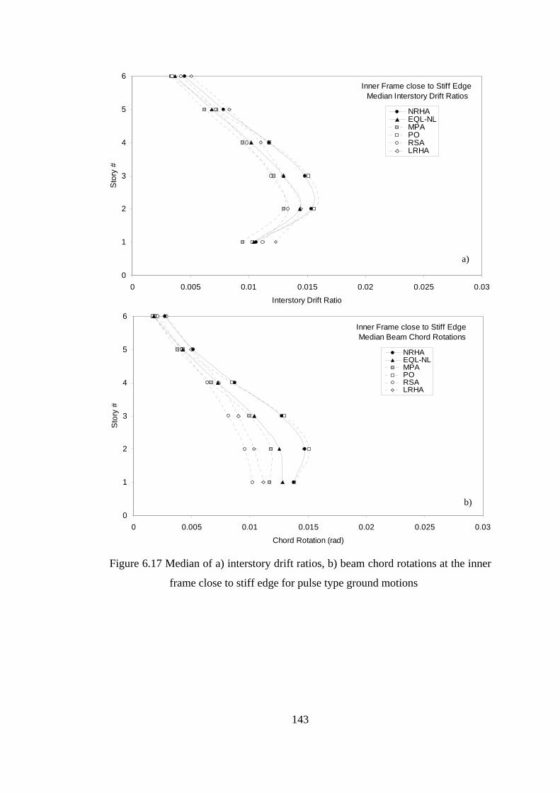
143
Figure 6.17 Median of a) interstory drift ratios, b) beam chord rotations at the inner
frame close to stiff edge for pulse type ground motions
0
1
2
3
4
5
6
0 0.005 0.01 0.015 0.02 0.025 0.03
Interstory Drift Ratio
Sto
ry #
Inner Frame close to Stiff Edge Median Interstory Drift Ratios
NRHAEQL-NLMPAPORSALRHA
0
1
2
3
4
5
6
0 0.005 0.01 0.015 0.02 0.025 0.03
Chord Rotation (rad)
Sto
ry #
Inner Frame close to Stiff Edge Median Beam Chord Rotations
NRHAEQL-NLMPAPORSALRHA
a)
b)
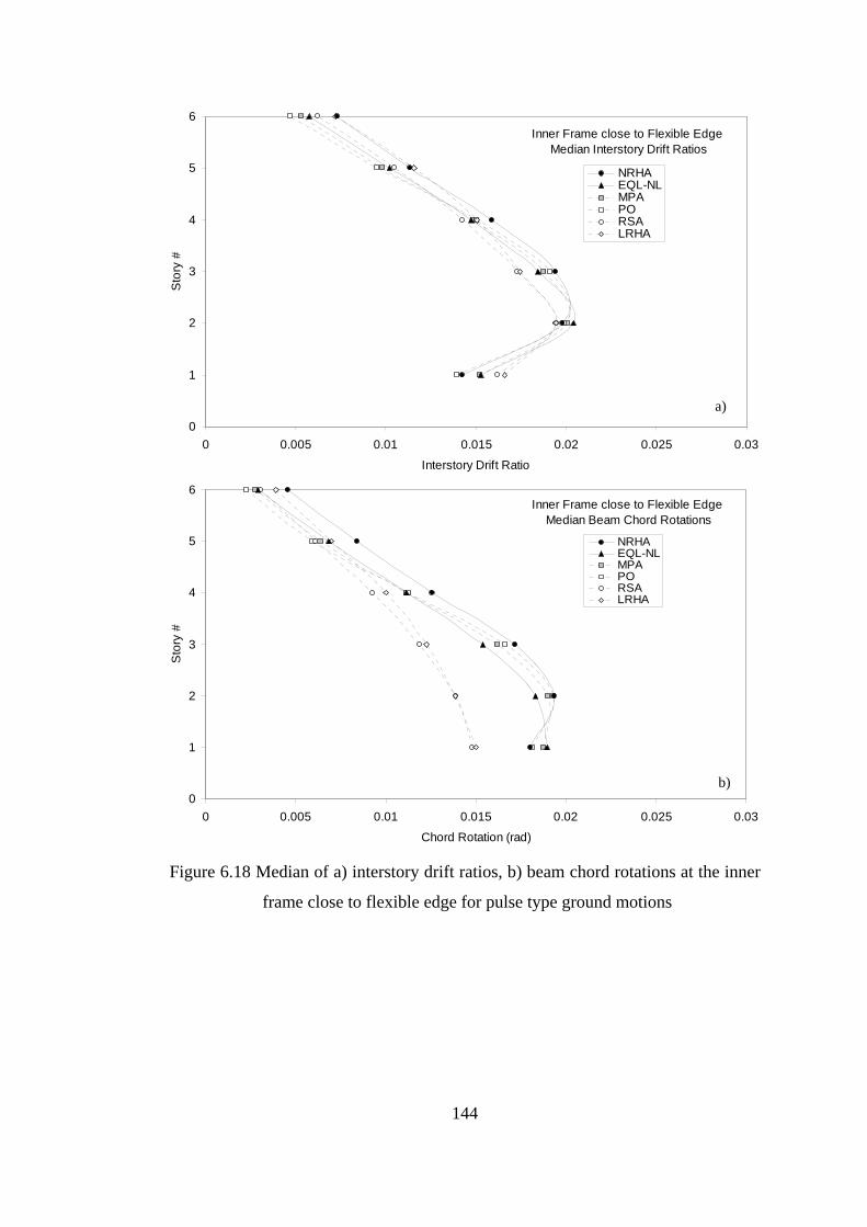
144
Figure 6.18 Median of a) interstory drift ratios, b) beam chord rotations at the inner
frame close to flexible edge for pulse type ground motions
0
1
2
3
4
5
6
0 0.005 0.01 0.015 0.02 0.025 0.03
Interstory Drift Ratio
Sto
ry #
Inner Frame close to Flexible Edge Median Interstory Drift Ratios
NRHAEQL-NLMPAPORSALRHA
0
1
2
3
4
5
6
0 0.005 0.01 0.015 0.02 0.025 0.03
Chord Rotation (rad)
Sto
ry #
Inner Frame close to Flexible Edge Median Beam Chord Rotations
NRHAEQL-NLMPAPORSALRHA
a)
b)
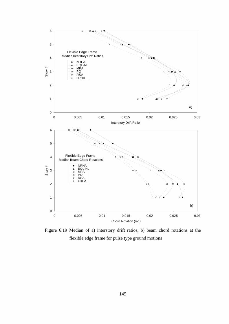
145
Figure 6.19 Median of a) interstory drift ratios, b) beam chord rotations at the
flexible edge frame for pulse type ground motions
0
1
2
3
4
5
6
0 0.005 0.01 0.015 0.02 0.025 0.03
Interstory Drift Ratio
Sto
ry #
Flexible Edge Frame Median Interstory Drift Ratios
NRHAEQL-NLMPAPORSALRHA
0
1
2
3
4
5
6
0 0.005 0.01 0.015 0.02 0.025 0.03
Chord Rotation (rad)
Sto
ry #
Flexible Edge Frame Median Beam Chord Rotations
NRHAEQL-NLMPAPORSALRHA
a)
b)
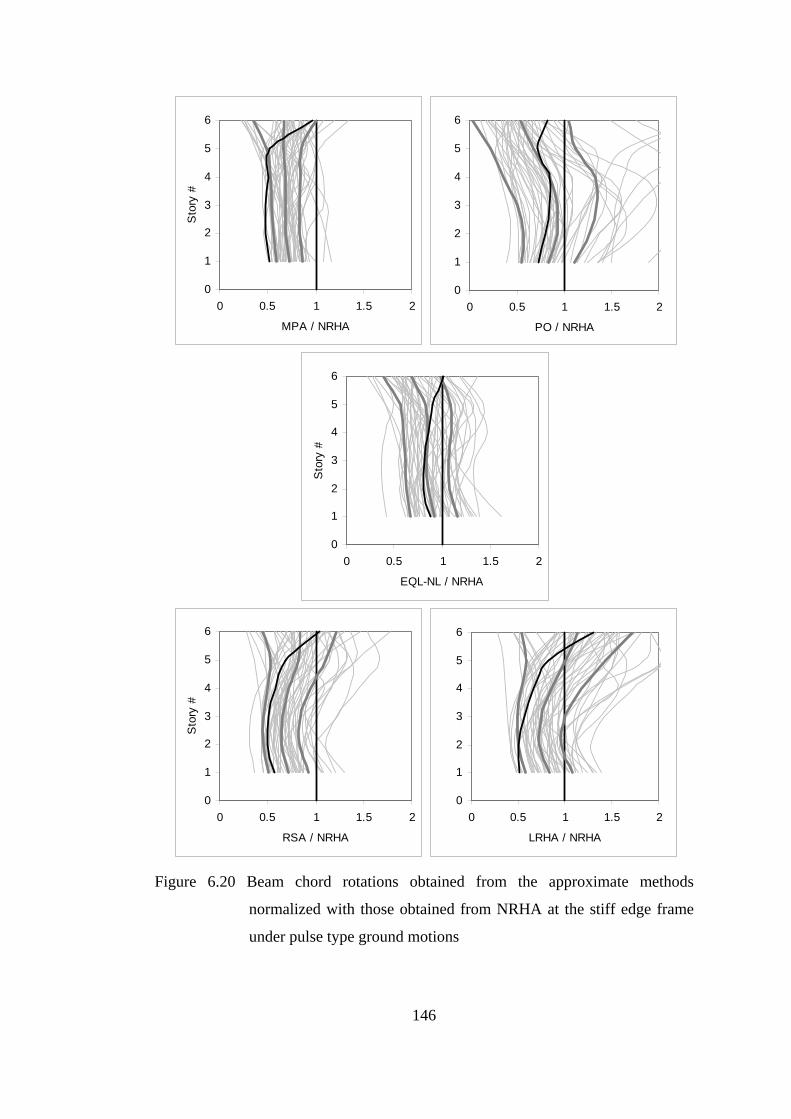
146
Figure 6.20 Beam chord rotations obtained from the approximate methods
normalized with those obtained from NRHA at the stiff edge frame
under pulse type ground motions
0
1
2
3
4
5
6
0 0.5 1 1.5 2
PO / NRHA
0
1
2
3
4
5
6
0 0.5 1 1.5 2
MPA / NRHA
Sto
ry #
0
1
2
3
4
5
6
0 0.5 1 1.5 2
EQL-NL / NRHA
Sto
ry #
0
1
2
3
4
5
6
0 0.5 1 1.5 2
RSA / NRHA
Sto
ry #
0
1
2
3
4
5
6
0 0.5 1 1.5 2
LRHA / NRHA
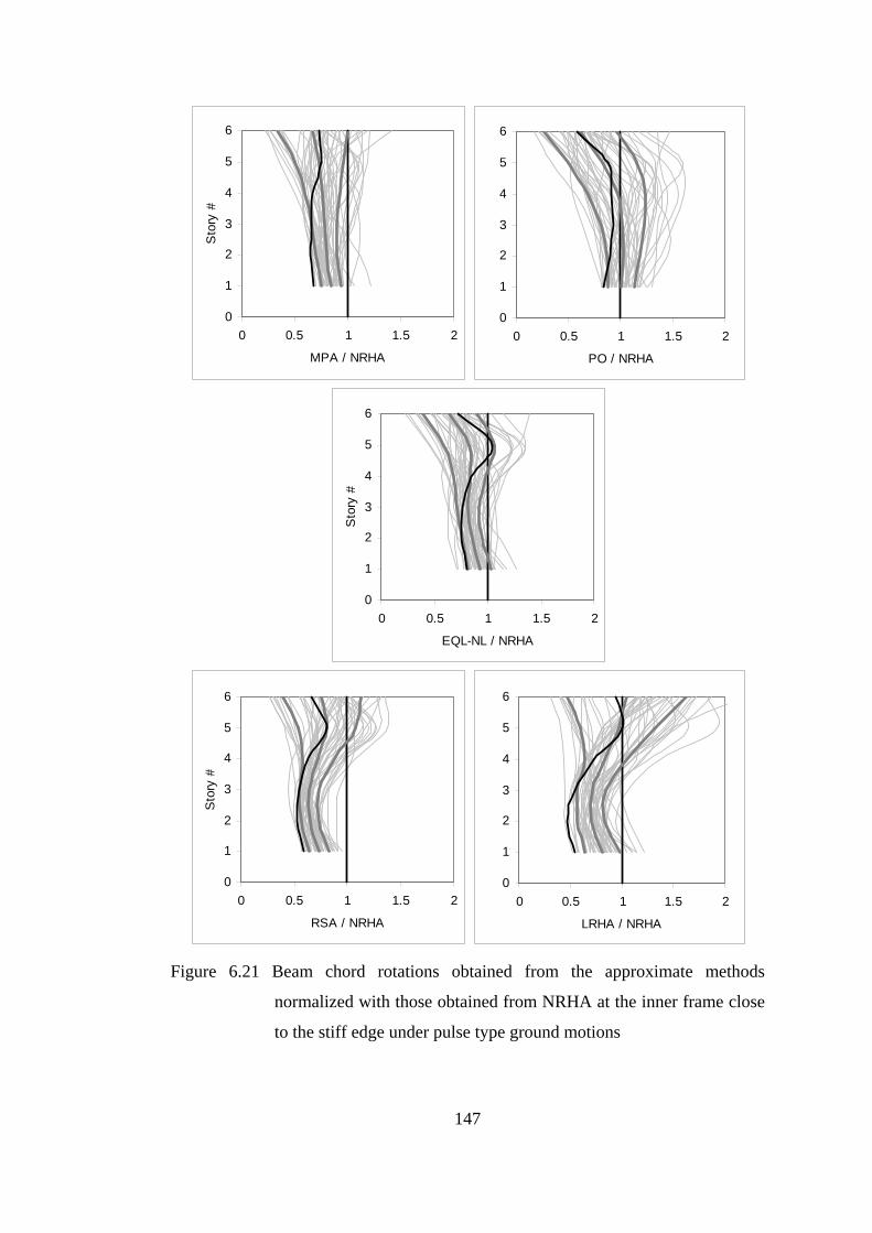
147
Figure 6.21 Beam chord rotations obtained from the approximate methods
normalized with those obtained from NRHA at the inner frame close
to the stiff edge under pulse type ground motions
0
1
2
3
4
5
6
0 0.5 1 1.5 2
PO / NRHA
0
1
2
3
4
5
6
0 0.5 1 1.5 2
MPA / NRHA
Sto
ry #
0
1
2
3
4
5
6
0 0.5 1 1.5 2
EQL-NL / NRHA
Sto
ry #
0
1
2
3
4
5
6
0 0.5 1 1.5 2
RSA / NRHA
Sto
ry #
0
1
2
3
4
5
6
0 0.5 1 1.5 2
LRHA / NRHA
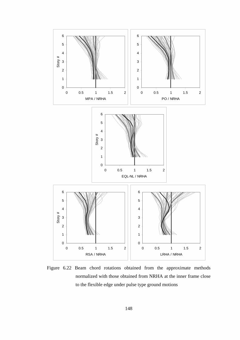
148
Figure 6.22 Beam chord rotations obtained from the approximate methods
normalized with those obtained from NRHA at the inner frame close
to the flexible edge under pulse type ground motions
0
1
2
3
4
5
6
0 0.5 1 1.5 2
PO / NRHA
0
1
2
3
4
5
6
0 0.5 1 1.5 2
MPA / NRHA
Sto
ry #
0
1
2
3
4
5
6
0 0.5 1 1.5 2
EQL-NL / NRHA
Sto
ry #
0
1
2
3
4
5
6
0 0.5 1 1.5 2
RSA / NRHA
Sto
ry #
0
1
2
3
4
5
6
0 0.5 1 1.5 2
LRHA / NRHA
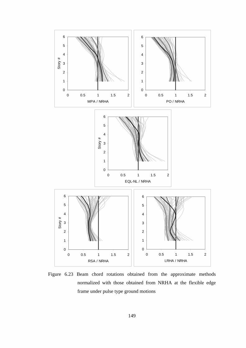
149
Figure 6.23 Beam chord rotations obtained from the approximate methods
normalized with those obtained from NRHA at the flexible edge
frame under pulse type ground motions
0
1
2
3
4
5
6
0 0.5 1 1.5 2
PO / NRHA
0
1
2
3
4
5
6
0 0.5 1 1.5 2
MPA / NRHA
Sto
ry #
0
1
2
3
4
5
6
0 0.5 1 1.5 2
EQL-NL / NRHA
Sto
ry #
0
1
2
3
4
5
6
0 0.5 1 1.5 2
RSA / NRHA
Sto
ry #
0
1
2
3
4
5
6
0 0.5 1 1.5 2
LRHA / NRHA

150
b) Ordinary Ground Motions
Median of interstory drift ratios and beam chord rotations obtained from the
employed analysis methods are plotted in Figures 6.24-6.27 for all of the frames of
the case study building under ordinary ground motions. Beam chord rotations
obtained from the approximate methods divided by those obtained from NRHA are
plotted in Figures 6.28-6.31. Observations related to these figures are very similar
to those noted from the pulse type ground motions.
• Equivalent linearization procedure is successful in improving the median
predictions of RSA for all the frames. Improvement in the beam chord
rotation estimations is more pronounced than the improvement in the
interstory drift ratios. There is considerable improvement in the beam chord
rotations of the flexible edge frame and the inner frame close to the flexible
edge.
• Observing the dispersion in the beam chord rotations in Figures 6.28-6.31, it
can be stated that EQL-NL results in similar values of scatter with RSA.
Therefore EQL-NL reduces the errors of RSA since it improves the median
predictions.
• Generally, RSA and LRHA underestimate the beam chord rotations and
interstory drift ratios. LRHA overestimates the top two story responses. As
can be seen from Figures 6.28-6.31, there are substantial differences between
the beam chord rotation predictions of RSA and LRHA because of the
differences in the consideration of torsional components of the modal forces.
• PO results in accurate predictions at the lower three stories of the frame at the
inner frame close to the stiff edge, inner frame close to the flexible edge and
the flexible edge frame. It underestimates the responses at the top three
stories. Equivalent linearization procedure results in better predictions than
PO at the top three stories of all frames. It also results in better beam chord
rotation predictions at the lower three stories of the stiff edge frame. EQL-NL
and PO results in similar errors in the beam chord rotation predictions at the
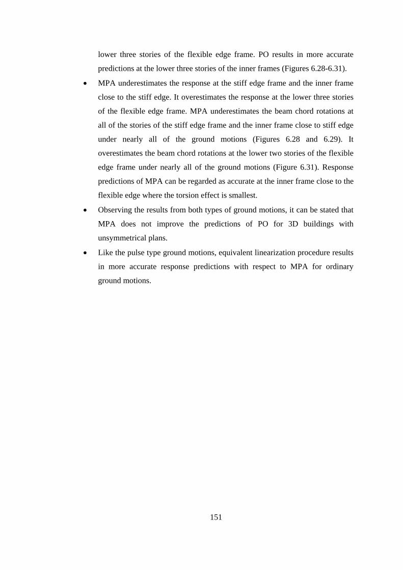
151
lower three stories of the flexible edge frame. PO results in more accurate
predictions at the lower three stories of the inner frames (Figures 6.28-6.31).
• MPA underestimates the response at the stiff edge frame and the inner frame
close to the stiff edge. It overestimates the response at the lower three stories
of the flexible edge frame. MPA underestimates the beam chord rotations at
all of the stories of the stiff edge frame and the inner frame close to stiff edge
under nearly all of the ground motions (Figures 6.28 and 6.29). It
overestimates the beam chord rotations at the lower two stories of the flexible
edge frame under nearly all of the ground motions (Figure 6.31). Response
predictions of MPA can be regarded as accurate at the inner frame close to the
flexible edge where the torsion effect is smallest.
• Observing the results from both types of ground motions, it can be stated that
MPA does not improve the predictions of PO for 3D buildings with
unsymmetrical plans.
• Like the pulse type ground motions, equivalent linearization procedure results
in more accurate response predictions with respect to MPA for ordinary
ground motions.
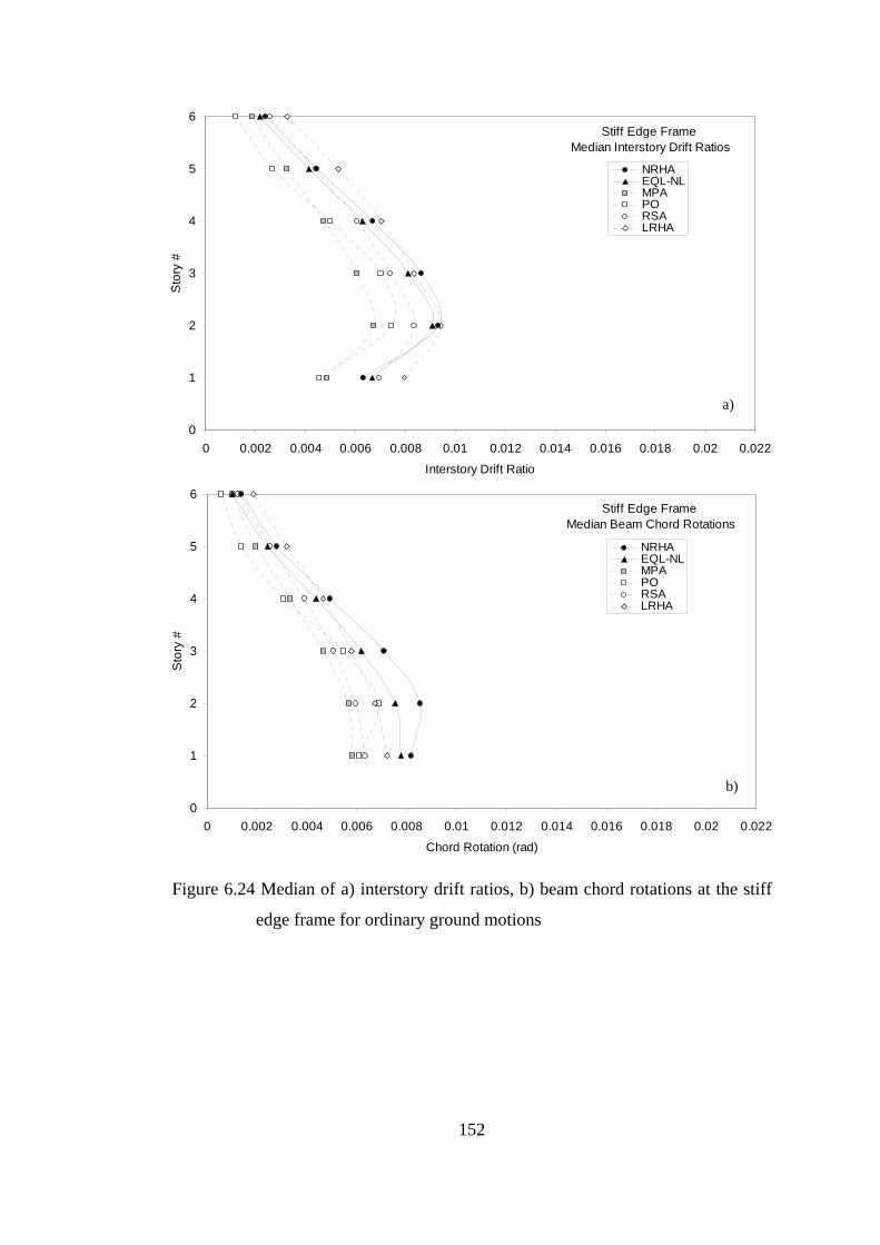
152
Figure 6.24 Median of a) interstory drift ratios, b) beam chord rotations at the stiff
edge frame for ordinary ground motions
0
1
2
3
4
5
6
0 0.002 0.004 0.006 0.008 0.01 0.012 0.014 0.016 0.018 0.02 0.022
Interstory Drift Ratio
Sto
ry #
Stiff Edge Frame Median Interstory Drift Ratios
NRHAEQL-NLMPAPORSALRHA
0
1
2
3
4
5
6
0 0.002 0.004 0.006 0.008 0.01 0.012 0.014 0.016 0.018 0.02 0.022
Chord Rotation (rad)
Sto
ry #
Stiff Edge Frame Median Beam Chord Rotations
NRHAEQL-NLMPAPORSALRHA
a)
b)
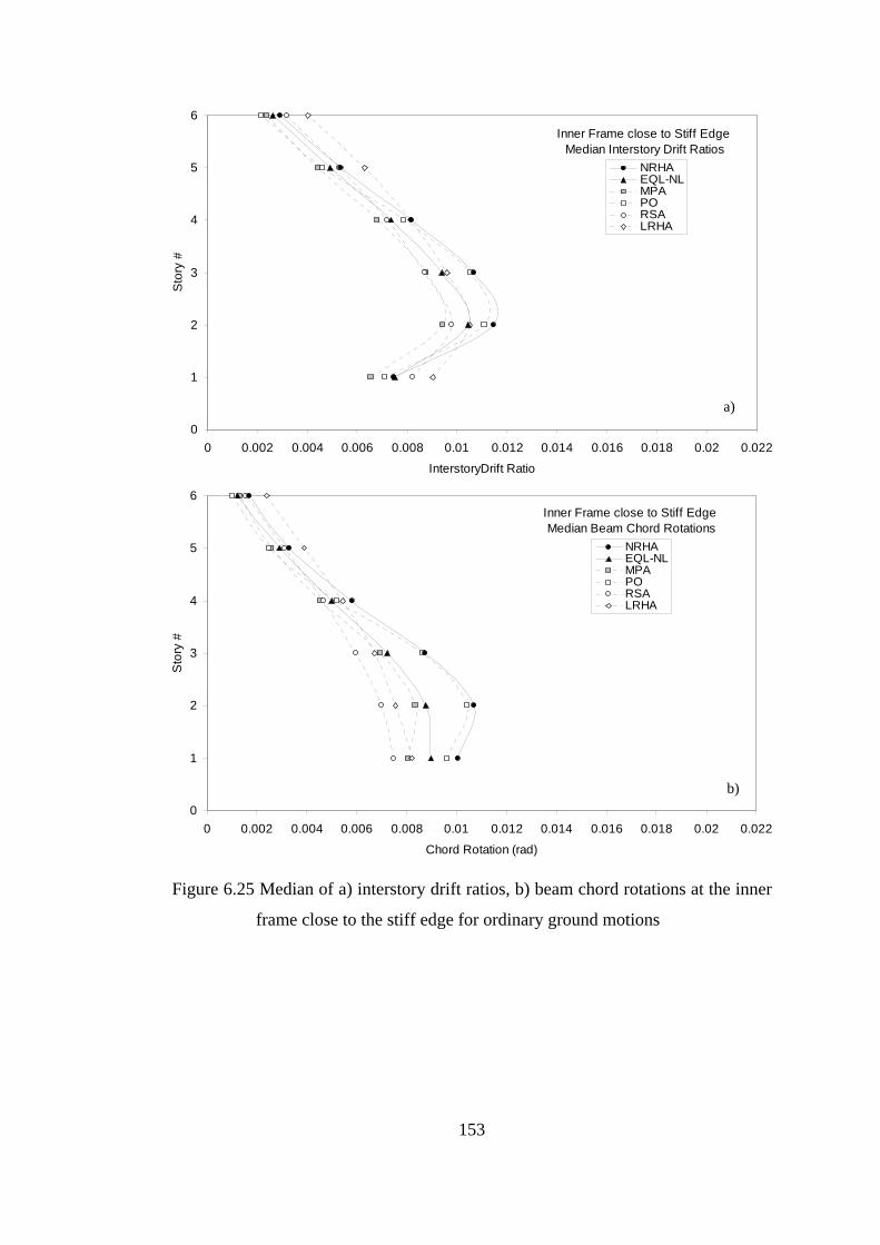
153
Figure 6.25 Median of a) interstory drift ratios, b) beam chord rotations at the inner
frame close to the stiff edge for ordinary ground motions
0
1
2
3
4
5
6
0 0.002 0.004 0.006 0.008 0.01 0.012 0.014 0.016 0.018 0.02 0.022
InterstoryDrift Ratio
Sto
ry #
Inner Frame close to Stiff Edge Median Interstory Drift Ratios
NRHAEQL-NLMPAPORSALRHA
0
1
2
3
4
5
6
0 0.002 0.004 0.006 0.008 0.01 0.012 0.014 0.016 0.018 0.02 0.022
Chord Rotation (rad)
Sto
ry #
Inner Frame close to Stiff Edge Median Beam Chord Rotations
NRHAEQL-NLMPAPORSALRHA
a)
b)
154
Figure 6.26 Median of a) interstory drift ratios, b) beam chord rotations at the inner
frame close to the flexible edge for ordinary ground motions
0
1
2
3
4
5
6
0 0.002 0.004 0.006 0.008 0.01 0.012 0.014 0.016 0.018 0.02 0.022
Intestory Drift Ratio
Sto
ry #
Inner Frame close to Flexible Edge Median Interstory Drift Ratios
NRHAEQL-NLMPAPORSALRHA
0
1
2
3
4
5
6
0 0.002 0.004 0.006 0.008 0.01 0.012 0.014 0.016 0.018 0.02 0.022
Chord Rotation (rad)
Sto
ry #
Inner Frame close to Flexible Edge Median Beam Chord Rotations
NRHAEQL-NLMPAPORSALRHA
a)
b)
155
Figure 6.27 Median of a) interstory drift ratios, b) beam chord rotations at the
flexible edge frame for ordinary ground motions
0
1
2
3
4
5
6
0 0.002 0.004 0.006 0.008 0.01 0.012 0.014 0.016 0.018 0.02 0.022
Chord Rotation (rad)
Sto
ry #
Flexible Edge Frame Median Beam Chord Rotations
NRHAEQL-NLMPAPORSALRHA
0
1
2
3
4
5
6
0 0.002 0.004 0.006 0.008 0.01 0.012 0.014 0.016 0.018 0.02 0.022
Interstory Drift Ratio
Sto
ry #
Flexible Edge Frame Median Interstory Drift Ratios
NRHAEQL-NLMPAPORSALRHA
a)
b)
156
Figure 6.28 Beam chord rotations obtained from the approximate methods
normalized with those obtained from NRHA at the stiff edge frame
under ordinary ground motions
0
1
2
3
4
5
6
0 0.5 1 1.5 2
PO / NRHA
0
1
2
3
4
5
6
0 0.5 1 1.5 2
MPA / NRHA
Sto
ry #
0
1
2
3
4
5
6
0 0.5 1 1.5 2
EQL-NL / NRHA
Sto
ry #
0
1
2
3
4
5
6
0 0.5 1 1.5 2
RSA / NRHA
Sto
ry #
0
1
2
3
4
5
6
0 0.5 1 1.5 2
LRHA / NRHA
157
Figure 6.29 Beam chord rotations obtained from the approximate methods
normalized with those obtained from NRHA at the inner frame close
to stiff edge under ordinary ground motions
0
1
2
3
4
5
6
0 0.5 1 1.5 2
PO / NRHA
0
1
2
3
4
5
6
0 0.5 1 1.5 2
MPA / NRHA
Sto
ry #
0
1
2
3
4
5
6
0 0.5 1 1.5 2
EQL-NL / NRHA
Sto
ry #
0
1
2
3
4
5
6
0 0.5 1 1.5 2
RSA / NRHA
Sto
ry #
0
1
2
3
4
5
6
0 0.5 1 1.5 2
LRHA / NRHA
158
Figure 6.30 Beam chord rotations obtained from the approximate methods
normalized with those obtained from NRHA at the inner frame close
to flexible edge under ordinary ground motions
0
1
2
3
4
5
6
0 0.5 1 1.5 2
PO / NRHA
0
1
2
3
4
5
6
0 0.5 1 1.5 2
MPA / NRHA
Sto
ry #
0
1
2
3
4
5
6
0 0.5 1 1.5 2
EQL-NL / NRHA
Sto
ry #
0
1
2
3
4
5
6
0 0.5 1 1.5 2
RSA / NRHA
Sto
ry #
0
1
2
3
4
5
6
0 0.5 1 1.5 2
LRHA / NRHA
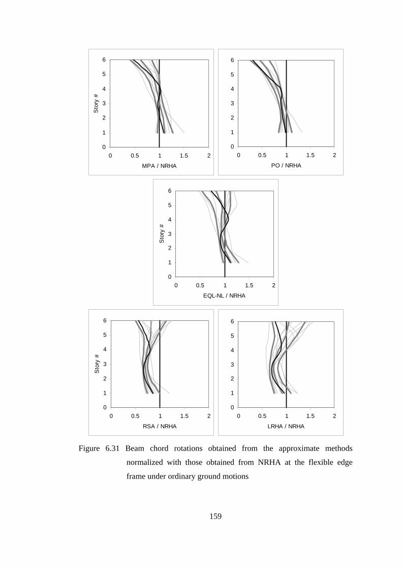
159
Figure 6.31 Beam chord rotations obtained from the approximate methods
normalized with those obtained from NRHA at the flexible edge
frame under ordinary ground motions
0
1
2
3
4
5
6
0 0.5 1 1.5 2
PO / NRHA
0
1
2
3
4
5
6
0 0.5 1 1.5 2
MPA / NRHA
Sto
ry #
0
1
2
3
4
5
6
0 0.5 1 1.5 2
EQL-NL / NRHA
Sto
ry #
0
1
2
3
4
5
6
0 0.5 1 1.5 2
RSA / NRHA
Sto
ry #
0
1
2
3
4
5
6
0 0.5 1 1.5 2
LRHA / NRHA
160
6.4.3 Response Prediction Under a Pulse Type Ground Motion
The proposed equivalent linearization procedure is evaluated in comparison
with other analysis methods under a pulse type ground motion in this section. Each
method is evaluated at the center of mass roof displacement determined by NRHA
as in the case of the statistical evaluations presented previously.
The ground motion selected as a pulse type example is the one with the code
SYL360 in Table 4.1. It is a strong ground motion recorded during 1994 Northridge
earthquake with PGA, PGV and PGD of 0.843 g, 129.4 cm/sec and 31.9 cm
respectively. Ground acceleration, velocity and displacement traces of this ground
motion are presented in Figure 6.32. Existence of strong pulses can be identified
from this figure. Pseudo acceleration and displacement response spectra of the
ground motion are presented in Figure 6.33. First and second mode periods are also
marked on these figures. The reason for selecting this ground motion is that it
results in considerable amount of nonlinearity and torsional response.
Comparison of maximum story displacements, interstory drift ratios and beam
chord rotations obtained from several analysis methods under the selected pulse
type ground motion are presented in Figures 6.34-6.39. Following observations can
be noted from these figures.
• Equivalent linearization procedure improves the predictions of RSA.
Improvement is clearly observed in the beam chord rotations. Since the beam
chord rotation is a better indicator of structural damage than interstory drift
ratio and story displacement, accurate prediction of beam chord rotations is an
achievement of the equivalent linearization procedure for assessment
purposes.
• Increase in the beam chord rotations and interstory drift ratios at the top two
stories of the flexible edge frame resembling the effect of higher modes is best
captured by the equivalent linearization procedure among the considered
approximate methods.
• LRHA and RSA result in substantially different interstory drift ratios and
beam chord rotations at the flexible edge frame because of the differences in

161
the consideration of the torsional components of the modal force vectors as
indicated previously.
• All of the methods underestimate the responses at the stiff edge, MPA
resulting in the largest underestimations. MPA greatly underestimates the
displacements, interstory drift ratios and beam chord rotations at the stiff edge
frame and overestimates the displacements at the flexible edge frame. It also
overestimates the interstory drift ratios and beam chord rotations at the lower
three stories which was previously observed for the statistical results. This
situation is because of the overestimation of torsion as explained previously.
• PO results in very accurate displacements at the flexible edge. It results in
underestimations for the other cases.
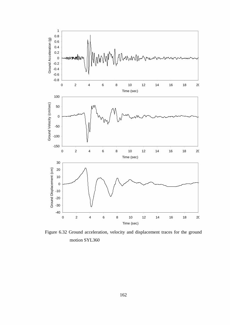
162
Figure 6.32 Ground acceleration, velocity and displacement traces for the ground
motion SYL360
-0.8-0.6-0.4-0.2
00.20.40.60.8
1
0 2 4 6 8 10 12 14 16 18 20
Time (sec)
Gro
und
Acc
eler
atio
n (g
)
-150
-100
-50
0
50
100
0 2 4 6 8 10 12 14 16 18 20
Time (sec)
Gro
und
Vel
ocity
(cm
/sec
)
-40
-30
-20
-10
0
10
20
30
0 2 4 6 8 10 12 14 16 18 20
Time (sec)
Gro
und
Dis
plac
emen
t (cm
)
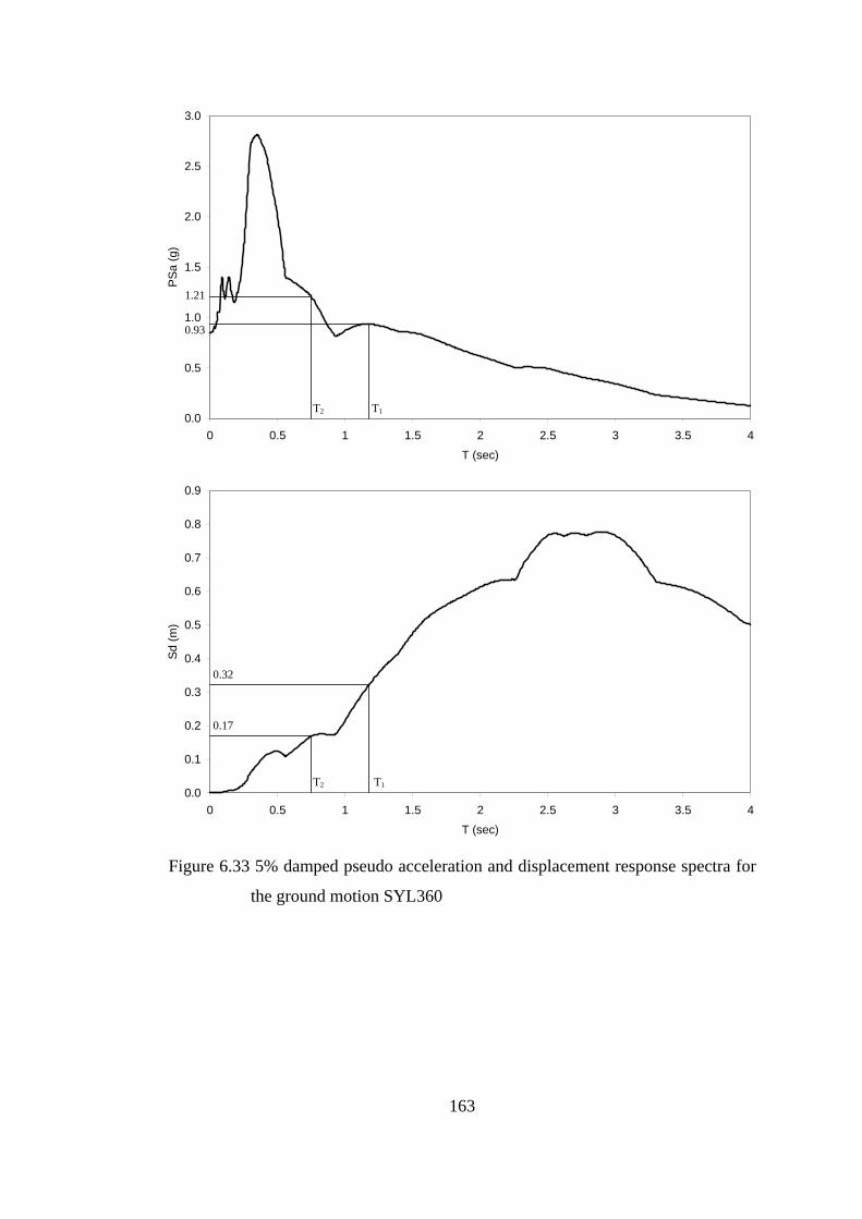
163
Figure 6.33 5% damped pseudo acceleration and displacement response spectra for
the ground motion SYL360
0.0
0.5
1.0
1.5
2.0
2.5
3.0
0 0.5 1 1.5 2 2.5 3 3.5 4T (sec)
PSa
(g)
0.0
0.1
0.2
0.3
0.4
0.5
0.6
0.7
0.8
0.9
0 0.5 1 1.5 2 2.5 3 3.5 4T (sec)
Sd (m
)
T1 T2
T1 T2
1.21
0.93
0.32
0.17

164
Figure 6.34 Comparison of maximum story displacements a) at the stiff edge frame,
b) at the inner frame close to the stiff edge for the ground motion
SYL360
0
1
2
3
4
5
6
0 0.05 0.1 0.15 0.2 0.25 0.3 0.35 0.4 0.45 0.5
Displacement (m)
Sto
ry #
NRHAEQL-NLMPAPORSALRHA
Stiff Edge Frame Displacements
0
1
2
3
4
5
6
0 0.05 0.1 0.15 0.2 0.25 0.3 0.35 0.4 0.45 0.5
Displacement (m)
Sto
ry #
Inner Frame close to Stiff Edge Displacements
NRHAEQL-NLMPAPORSALRHA
a)
b)
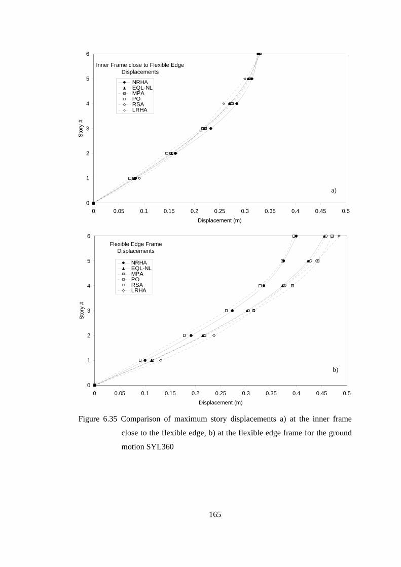
165
Figure 6.35 Comparison of maximum story displacements a) at the inner frame
close to the flexible edge, b) at the flexible edge frame for the ground
motion SYL360
0
1
2
3
4
5
6
0 0.05 0.1 0.15 0.2 0.25 0.3 0.35 0.4 0.45 0.5
Displacement (m)
Sto
ry #
Inner Frame close to Flexible Edge Displacements
NRHAEQL-NLMPAPORSALRHA
0
1
2
3
4
5
6
0 0.05 0.1 0.15 0.2 0.25 0.3 0.35 0.4 0.45 0.5
Displacement (m)
Sto
ry #
Flexible Edge Frame Displacements
NRHAEQL-NLMPAPORSALRHA
a)
b)
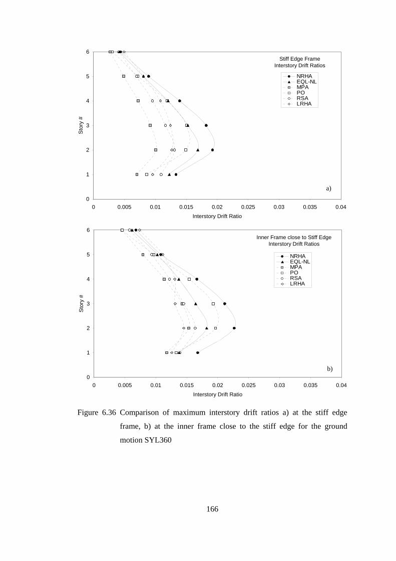
166
Figure 6.36 Comparison of maximum interstory drift ratios a) at the stiff edge
frame, b) at the inner frame close to the stiff edge for the ground
motion SYL360
0
1
2
3
4
5
6
0 0.005 0.01 0.015 0.02 0.025 0.03 0.035 0.04Interstory Drift Ratio
Sto
ry #
Stiff Edge Frame Interstory Drift Ratios
NRHAEQL-NLMPAPORSALRHA
0
1
2
3
4
5
6
0 0.005 0.01 0.015 0.02 0.025 0.03 0.035 0.04Interstory Drift Ratio
Sto
ry #
Inner Frame close to Stiff Edge Interstory Drift Ratios
NRHAEQL-NLMPAPORSALRHA
a)
b)
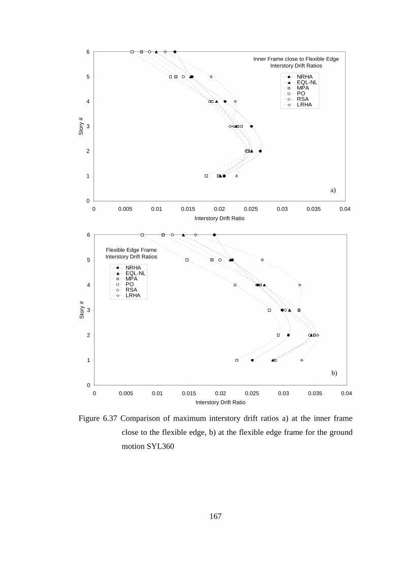
167
Figure 6.37 Comparison of maximum interstory drift ratios a) at the inner frame
close to the flexible edge, b) at the flexible edge frame for the ground
motion SYL360
0
1
2
3
4
5
6
0 0.005 0.01 0.015 0.02 0.025 0.03 0.035 0.04Interstory Drift Ratio
Sto
ry #
Inner Frame close to Flexible Edge Interstory Drift Ratios
NRHAEQL-NLMPAPORSALRHA
0
1
2
3
4
5
6
0 0.005 0.01 0.015 0.02 0.025 0.03 0.035 0.04Interstory Drift Ratio
Sto
ry #
Flexible Edge Frame Interstory Drift Ratios
NRHAEQL-NLMPAPORSALRHA
a)
b)
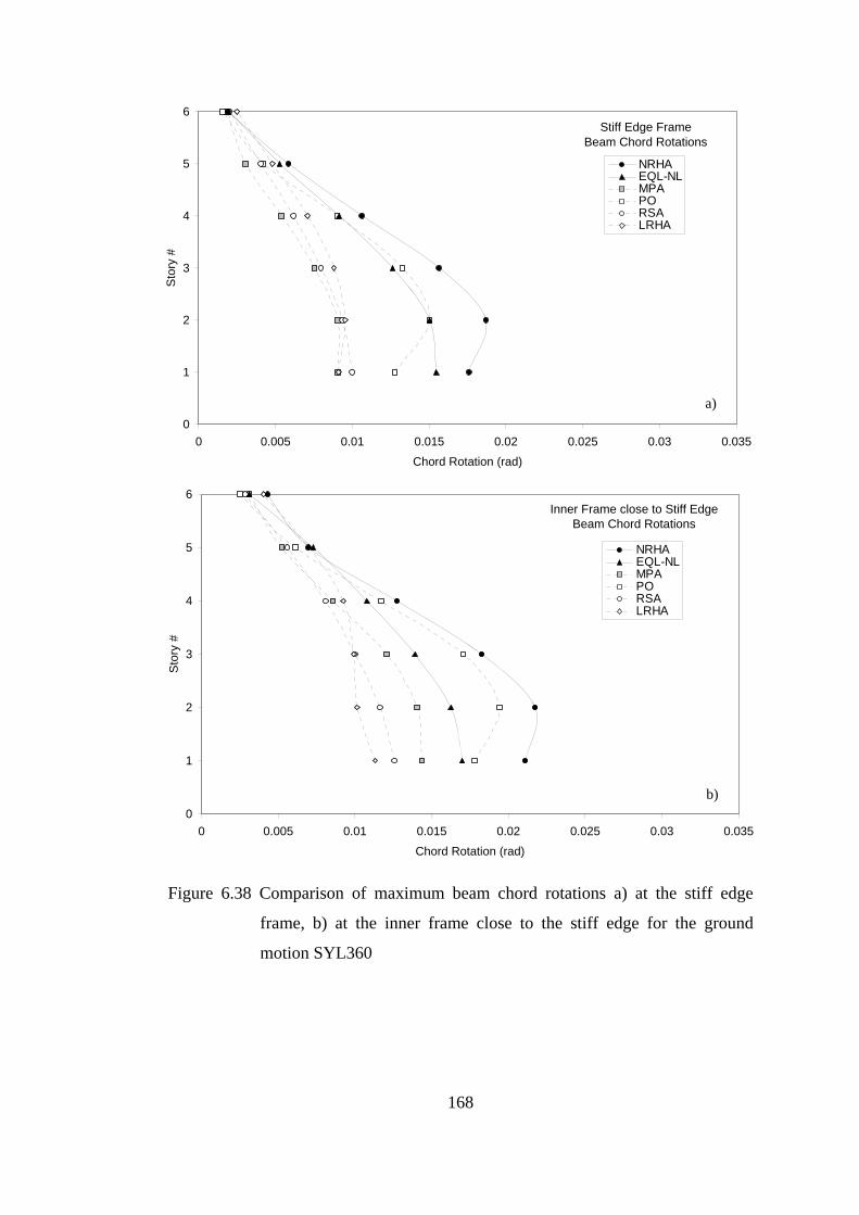
168
Figure 6.38 Comparison of maximum beam chord rotations a) at the stiff edge
frame, b) at the inner frame close to the stiff edge for the ground
motion SYL360
0
1
2
3
4
5
6
0 0.005 0.01 0.015 0.02 0.025 0.03 0.035
Chord Rotation (rad)
Sto
ry #
Inner Frame close to Stiff EdgeBeam Chord Rotations
NRHAEQL-NLMPAPORSALRHA
0
1
2
3
4
5
6
0 0.005 0.01 0.015 0.02 0.025 0.03 0.035
Chord Rotation (rad)
Sto
ry #
Stiff Edge Frame Beam Chord Rotations
NRHAEQL-NLMPAPORSALRHA
a)
b)
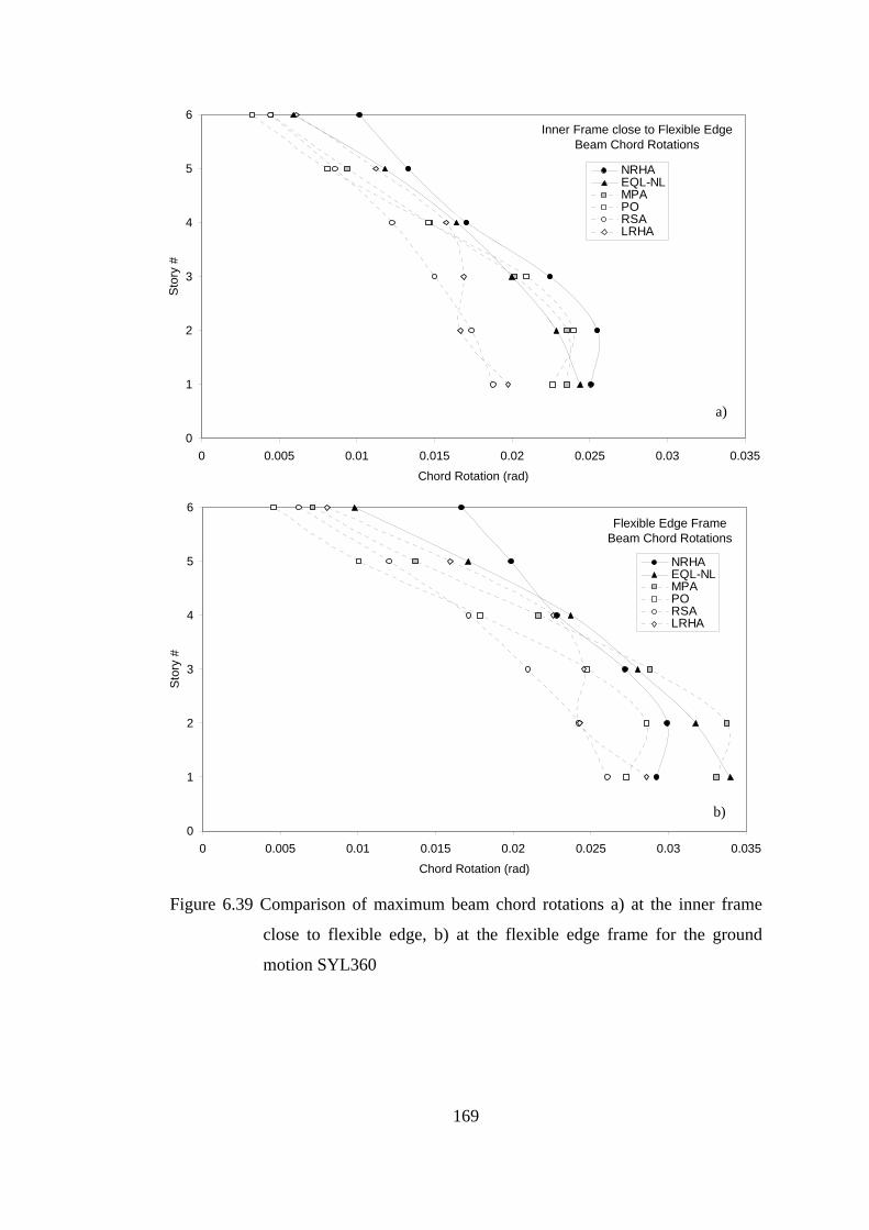
169
Figure 6.39 Comparison of maximum beam chord rotations a) at the inner frame
close to flexible edge, b) at the flexible edge frame for the ground
motion SYL360
0
1
2
3
4
5
6
0 0.005 0.01 0.015 0.02 0.025 0.03 0.035
Chord Rotation (rad)
Sto
ry #
Flexible Edge Frame Beam Chord Rotations
NRHAEQL-NLMPAPORSALRHA
0
1
2
3
4
5
6
0 0.005 0.01 0.015 0.02 0.025 0.03 0.035
Chord Rotation (rad)
Sto
ry #
NRHAEQL-NLMPAPORSALRHA
Inner Frame close to Flexible EdgeBeam Chord Rotations
a)
b)
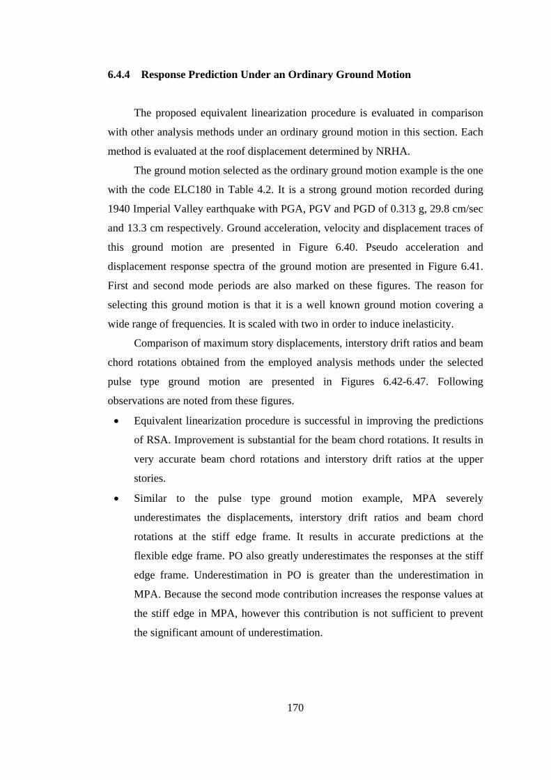
170
6.4.4 Response Prediction Under an Ordinary Ground Motion
The proposed equivalent linearization procedure is evaluated in comparison
with other analysis methods under an ordinary ground motion in this section. Each
method is evaluated at the roof displacement determined by NRHA.
The ground motion selected as the ordinary ground motion example is the one
with the code ELC180 in Table 4.2. It is a strong ground motion recorded during
1940 Imperial Valley earthquake with PGA, PGV and PGD of 0.313 g, 29.8 cm/sec
and 13.3 cm respectively. Ground acceleration, velocity and displacement traces of
this ground motion are presented in Figure 6.40. Pseudo acceleration and
displacement response spectra of the ground motion are presented in Figure 6.41.
First and second mode periods are also marked on these figures. The reason for
selecting this ground motion is that it is a well known ground motion covering a
wide range of frequencies. It is scaled with two in order to induce inelasticity.
Comparison of maximum story displacements, interstory drift ratios and beam
chord rotations obtained from the employed analysis methods under the selected
pulse type ground motion are presented in Figures 6.42-6.47. Following
observations are noted from these figures.
• Equivalent linearization procedure is successful in improving the predictions
of RSA. Improvement is substantial for the beam chord rotations. It results in
very accurate beam chord rotations and interstory drift ratios at the upper
stories.
• Similar to the pulse type ground motion example, MPA severely
underestimates the displacements, interstory drift ratios and beam chord
rotations at the stiff edge frame. It results in accurate predictions at the
flexible edge frame. PO also greatly underestimates the responses at the stiff
edge frame. Underestimation in PO is greater than the underestimation in
MPA. Because the second mode contribution increases the response values at
the stiff edge in MPA, however this contribution is not sufficient to prevent
the significant amount of underestimation.
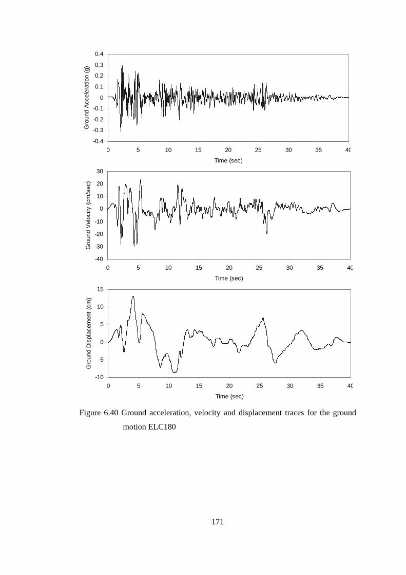
171
Figure 6.40 Ground acceleration, velocity and displacement traces for the ground
motion ELC180
-0.4
-0.3
-0.2
-0.1
0
0.1
0.2
0.3
0.4
0 5 10 15 20 25 30 35 40
Time (sec)
Gro
und
Acc
eler
atio
n (g
)
-40
-30
-20
-10
0
10
20
30
0 5 10 15 20 25 30 35 40
Time (sec)
Gro
und
Vel
ocity
(cm
/sec
)
-10
-5
0
5
10
15
0 5 10 15 20 25 30 35 40
Time (sec)
Gro
und
Dis
plac
emen
t (cm
)
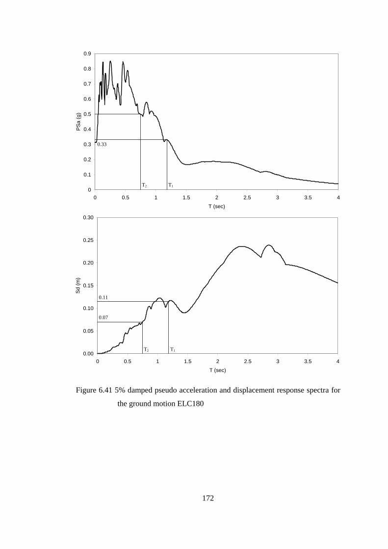
172
Figure 6.41 5% damped pseudo acceleration and displacement response spectra for
the ground motion ELC180
0
0.1
0.2
0.3
0.4
0.5
0.6
0.7
0.8
0.9
0 0.5 1 1.5 2 2.5 3 3.5 4T (sec)
PSa
(g)
0.00
0.05
0.10
0.15
0.20
0.25
0.30
0 0.5 1 1.5 2 2.5 3 3.5 4T (sec)
Sd (m
)
T1 T2
T1 T2
0.33
0.11
0.07
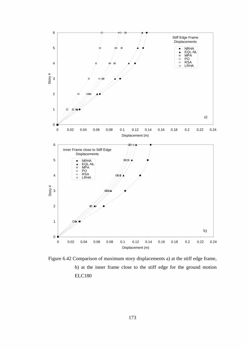
173
Figure 6.42 Comparison of maximum story displacements a) at the stiff edge frame,
b) at the inner frame close to the stiff edge for the ground motion
ELC180
0
1
2
3
4
5
6
0 0.02 0.04 0.06 0.08 0.1 0.12 0.14 0.16 0.18 0.2 0.22 0.24
Displacement (m)
Sto
ry #
NRHAEQL-NLMPAPORSALRHA
Stiff Edge Frame Displacements
0
1
2
3
4
5
6
0 0.02 0.04 0.06 0.08 0.1 0.12 0.14 0.16 0.18 0.2 0.22 0.24
Displacement (m)
Sto
ry #
NRHAEQL-NLMPAPORSALRHA
Inner Frame close to Stiff Edge Displacements
a)
b)
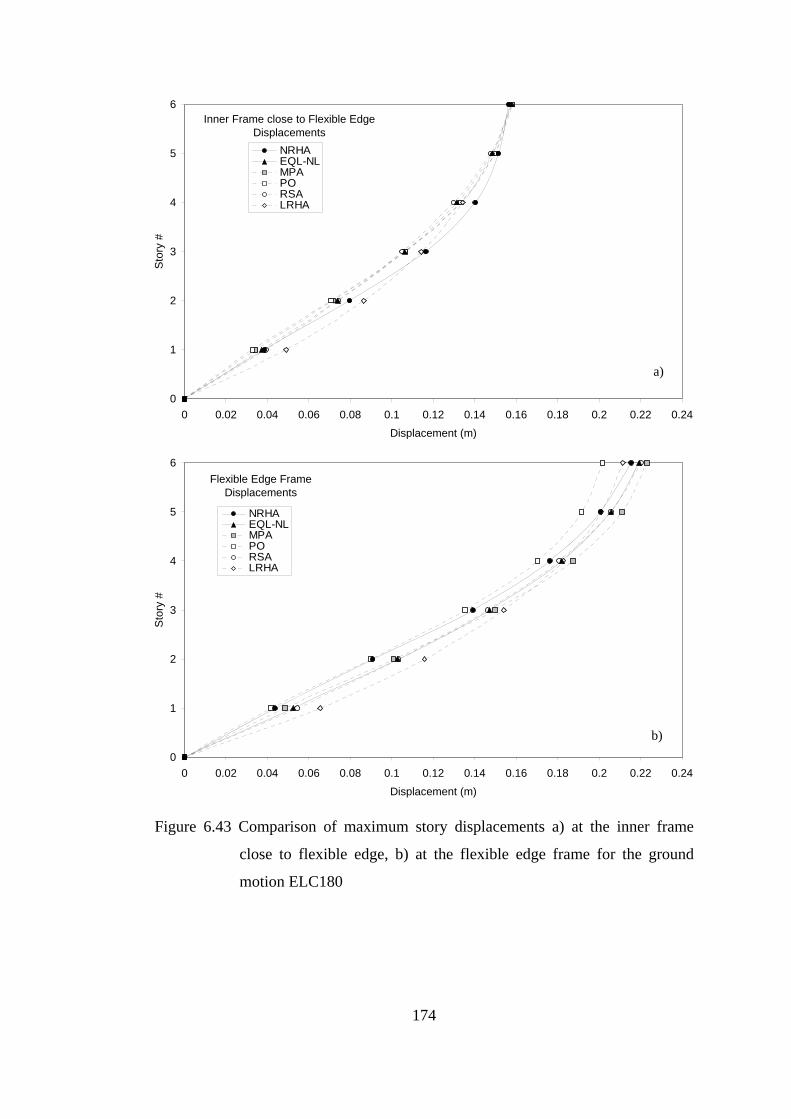
174
Figure 6.43 Comparison of maximum story displacements a) at the inner frame
close to flexible edge, b) at the flexible edge frame for the ground
motion ELC180
0
1
2
3
4
5
6
0 0.02 0.04 0.06 0.08 0.1 0.12 0.14 0.16 0.18 0.2 0.22 0.24
Displacement (m)
Sto
ry #
NRHAEQL-NLMPAPORSALRHA
Inner Frame close to Flexible Edge Displacements
0
1
2
3
4
5
6
0 0.02 0.04 0.06 0.08 0.1 0.12 0.14 0.16 0.18 0.2 0.22 0.24
Displacement (m)
Sto
ry #
NRHAEQL-NLMPAPORSALRHA
Flexible Edge Frame Displacements
a)
b)
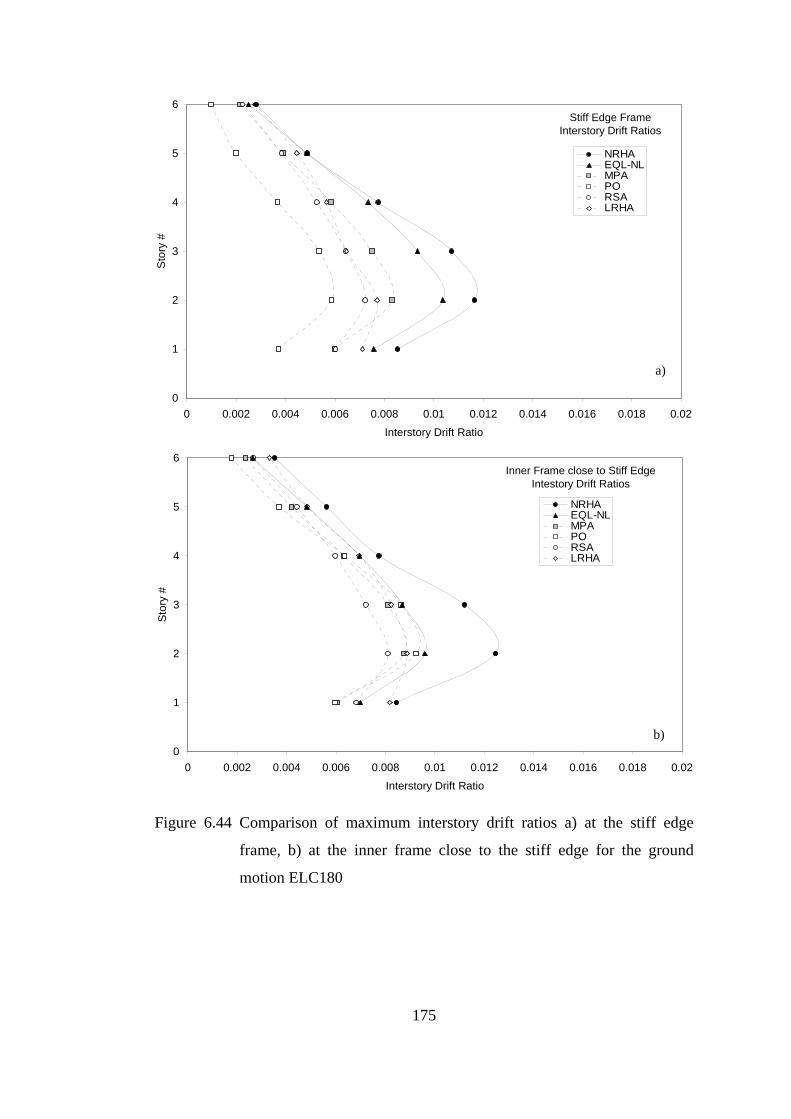
175
Figure 6.44 Comparison of maximum interstory drift ratios a) at the stiff edge
frame, b) at the inner frame close to the stiff edge for the ground
motion ELC180
0
1
2
3
4
5
6
0 0.002 0.004 0.006 0.008 0.01 0.012 0.014 0.016 0.018 0.02Interstory Drift Ratio
Sto
ry #
NRHAEQL-NLMPAPORSALRHA
Stiff Edge Frame Interstory Drift Ratios
0
1
2
3
4
5
6
0 0.002 0.004 0.006 0.008 0.01 0.012 0.014 0.016 0.018 0.02Interstory Drift Ratio
Sto
ry #
NRHAEQL-NLMPAPORSALRHA
Inner Frame close to Stiff EdgeIntestory Drift Ratios
a)
b)
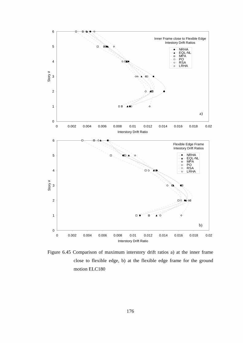
176
Figure 6.45 Comparison of maximum interstory drift ratios a) at the inner frame
close to flexible edge, b) at the flexible edge frame for the ground
motion ELC180
0
1
2
3
4
5
6
0 0.002 0.004 0.006 0.008 0.01 0.012 0.014 0.016 0.018 0.02Interstory Drift Ratio
Sto
ry #
NRHAEQL-NLMPAPORSALRHA
Inner Frame close to Flexible EdgeIntestory Drift Ratios
0
1
2
3
4
5
6
0 0.002 0.004 0.006 0.008 0.01 0.012 0.014 0.016 0.018 0.02Interstory Drift Ratio
Sto
ry #
NRHAEQL-NLMPAPORSALRHA
Flexible Edge Frame Intestory Drift Ratios
a)
b)
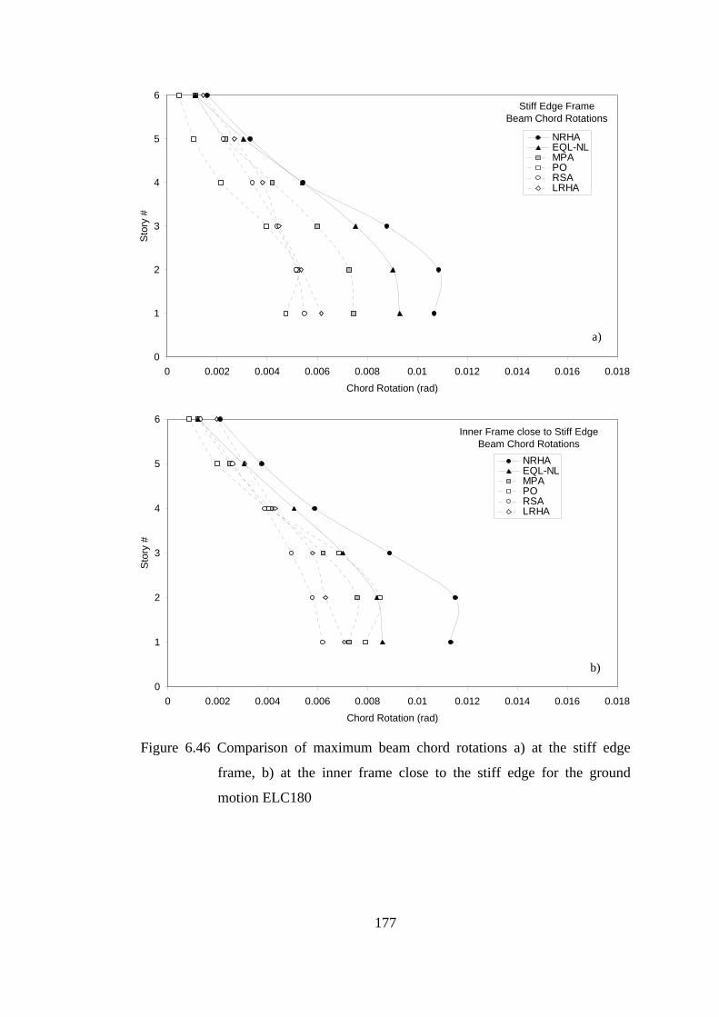
177
Figure 6.46 Comparison of maximum beam chord rotations a) at the stiff edge
frame, b) at the inner frame close to the stiff edge for the ground
motion ELC180
0
1
2
3
4
5
6
0 0.002 0.004 0.006 0.008 0.01 0.012 0.014 0.016 0.018
Chord Rotation (rad)
Sto
ry #
NRHAEQL-NLMPAPORSALRHA
Stiff Edge Frame Beam Chord Rotations
0
1
2
3
4
5
6
0 0.002 0.004 0.006 0.008 0.01 0.012 0.014 0.016 0.018
Chord Rotation (rad)
Sto
ry #
NRHAEQL-NLMPAPORSALRHA
Inner Frame close to Stiff Edge Beam Chord Rotations
a)
b)
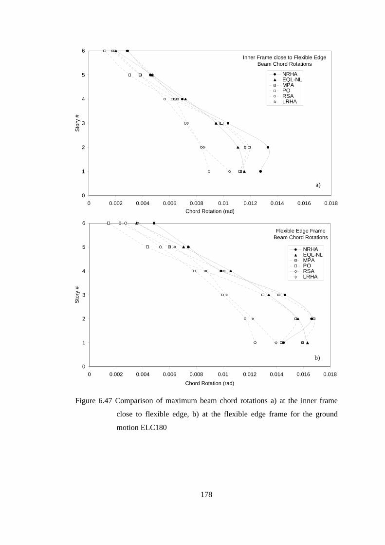
178
Figure 6.47 Comparison of maximum beam chord rotations a) at the inner frame
close to flexible edge, b) at the flexible edge frame for the ground
motion ELC180
0
1
2
3
4
5
6
0 0.002 0.004 0.006 0.008 0.01 0.012 0.014 0.016 0.018Chord Rotation (rad)
Sto
ry #
NRHAEQL-NLMPAPORSALRHA
Inner Frame close to Flexible Edge Beam Chord Rotations
0
1
2
3
4
5
6
0 0.002 0.004 0.006 0.008 0.01 0.012 0.014 0.016 0.018
Chord Rotation (rad)
Sto
ry #
NRHAEQL-NLMPAPORSALRHA
Flexible Edge Frame Beam Chord Rotations
a)
b)
179
CHAPTER 7
SUMMARY AND CONCLUSIONS
7.1 Summary
An equivalent linearization procedure is developed herein as an approximate
method for predicting the inelastic seismic displacement response of MDOF
systems under earthquake excitations. The procedure mainly consists of reducing
the stiffness of the structural members which are anticipated to respond in the
inelastic range. Combined results of demand and capacity analyses are used for the
construction of equivalent linear system with reduced stiffness. Different from
similar studies in literature, equivalent damping is not explicitly employed in this
study. Instead, predetermined spectral displacement demands are utilized in each
mode of the equivalent linear system for the determination of global displacement
demands. In the first variant of the equivalent linearization procedure (EQL-ED),
spectral displacements of all the modes are determined by means of the equal
displacement rule. In the second variant (EQL-NL), spectral displacement of only
the first mode is determined by conducting nonlinear response history analysis of an
equivalent SDOF system, different from EQL-ED. Modal response spectrum
analysis of the equivalent linear system is then conducted by using the pseudo
accelerations calculated from the spectral displacements, and the requested response
parameters are obtained.
180
Equivalent linearization procedure with both variants for calculating demand
(EQL-NL, EQL-ED) are applied on a twelve story reinforced concrete plane frame
for which the higher mode effects are important, and a six story unsymmetrical-plan
reinforced concrete space frame where torsion significantly effects the response.
The predictions of the equivalent linearization procedure are compared with the
nonlinear response history analysis (NRHA) results by utilizing 162 ground
motions. Response predictions from two other approximate procedures, which are
conventional pushover analysis according to FEMA-356 (PO-FEMA) and modal
pushover analysis (MPA) are also presented. Modal pushover analysis results
conducted by considering only the first mode (MPA-1) are also presented for the
twelve story building. In addition, results of response spectrum analyses (RSA) and
linear response history analyses (LRHA) are used for comparison purposes. Roof
displacement demands and the local response parameters; namely, story
displacements, interstory drift ratios and chord rotations are used in the
comparisons.
7.2 Conclusions
The following conclusions are reached according to the results obtained in
this study.
• EQL-NL is very successful in predicting the roof displacement demands. It
greatly improves the inaccurate predictions of RSA. The same conclusion is
not valid for EQL-ED. Roof displacement predictions of EQL-ED are close to
those of RSA, since same spectral displacements are employed in both of the
methods and the modal participation factors for the equivalent linear and the
original systems are similar. In this respect, it can be stated that EQL-NL is
superior to EQL-ED.
181
• Regarding the differences in the roof displacement demand predictions of
EQL-NL and EQL-ED, and the success of MPA in roof displacement
predictions, it is clear that the improvement in roof displacement prediction is
due to considering the inelastic response of SDOF systems instead of
employing the equal displacement assumption.
• Displacement demands of pulse type ground motions are much greater than
those demanded by ordinary ground motions. Considering that pulse type and
ordinary ground motions possess similar PGA levels, it can be concluded that
the pulses with high velocity peaks lead to the observed differences between
the displacement demands of pulse type and ordinary ground motions.
• Artificial axial forces develop in the beams despite the imposition of
diaphragm constraints when fiber sections are employed. Moment capacities
of the beams increase due to these artificial axial forces. Accordingly, a
building designed for beam yielding may result in a failure formation different
than the intended if the design is based on a model without fiber sections. This
is a critical issue for the nonlinear analysis of structures modeled by using
fiber sections, therefore it should be further investigated.
• For the twelve story plane frame, equivalent linearization procedure
significantly improves the inaccurate beam chord rotation and interstory drift
ratio predictions of RSA. Errors are greatly reduced at the upper stories at
which higher modes are effective on the response. Error of the equivalent
linearization procedure is much smaller than that of the first mode pushover
(MPA-1) at the upper stories. Generally, error of the equivalent linearization
procedure is between the error of RSA and MPA, being closer to the error of
MPA under pulse type ground motions where significant inelasticity
develops. Error of the equivalent linearization procedure is generally smaller
182
than that of MPA for all the considered response parameters under ordinary
ground motions which result in relatively smaller levels of inelasticity.
• Equivalent linearization procedure is also successful in predicting the beam
chord rotations and interstory drift ratios of the six story building with
unsymmetrical-plan. It improves the predictions of RSA. Improvement in the
beam chord rotations is more pronounced than the improvement in the
interstory drift ratios. There is considerable improvement in the beam chord
rotations at the flexible edge frame and the inner frame close to the flexible
edge where inelasticity is larger. Response predictions of the equivalent
linearization procedure have similar accuracy with the response predictions of
the conventional pushover analysis; in addition they are more accurate at the
top stories where higher mode effects are important. Equivalent linearization
procedure results in more accurate predictions of local response parameters
with respect to MPA.
• Owing to the results obtained from the two case study buildings, it is observed
that equivalent linearization procedure significantly improves the response
predictions of the response spectrum analysis. It also results in predictions
similar to or better than those obtained from the approximate methods which
employ nonlinear analysis. Considering the conceptual simplicity of the
procedure and the conventional analysis tools used in its application, it can be
stated that the equivalent linearization procedure is a practically applicable
method in the prediction of inelastic displacement response parameters with
sufficient accuracy.
• According to the response predictions of MPA for the six story building, it
can be stated that consideration of torques in the modal force vectors is a
drawback of MPA for 3D buildings with unsymmetrical plans. MPA is
successful in correcting the interstory drift ratios and beam chord rotations at
the upper stories predicted by the first mode pushover analysis (MPA-1) for

183
the twelve story plane frame. However, it leads to inaccurate response
predictions for the six story building because of the overestimation of torsion.
• Most of the improved pushover methods in literature are validated by using
2D models. It is essential that the accuracy of these methods should be
assessed by using 3D models.
184
REFERENCES Akkar S. and Metin A., 2007, ‘Assessment of Nonlinear Static Procedures in FEMA-440’, Journal of Structural Engineering, ASCE, Volume 133, No. 9, pp. 1237-1246
Akkar S. and Miranda E., 2005, ‘Statistical Evaluation of Approximate Methods for Estimating Maximum Deformation Demands on Existing Structures’, Journal of Structural Engineering, ASCE, Volume 131, No. 1, pp.160-172.
Akkar S., Yazgan U. and Gülkan P., 2005, ‘Drift Estimates in Frame Buildings Subjected to Near-Fault Ground Motions’, Journal of Structural Engineering, ASCE, Volume 131, No. 7, pp. 1014-1024.
Alavi B. and Krawinkler H., 2001, ‘Effects of Near-fault Ground Motions on Frame Structures’, John A. Blume Earthquake Engineering Center, Report No. 138, Stanford University.
Alavi B. and Krawinkler H., 2004, ‘Behaviour of Moment Resisting Frame Structures Subjected to Near-fault Ground Motions’, Earthquake Engineering and Structural Dynamics, Volume 33, pp. 687-706.
Allahabadi R. 1987, ‘Drain-2DX - Seismic Response and Damage Assessment for 2D structures’, Ph.D. Thesis, University of California, Berkeley, California.
American Society of Civil Engineers (ASCE), 2000, ‘Prestandard and Commentary for the Seismic Rehabilitation of Buildings’, Report No. FEMA-356, Washington, D.C.

185
Ang A.H.S. and Tang W.H., 1975, ‘Probability Concepts in Engineering Planning and Design, Volume I: Basic Principles’, Wiley, New York, 409 pp.
Antoniou S. and Pinho R., 2004a, ‘Advantages and Limitations of Adaptive and Non-Adaptive Force-Based Pushover Procedures’, Journal of Earthquake Engineering, Volume 8, No. 4, pp. 497-522.
Antoniou S. and Pinho R., 2004b, ‘Development and Verification of a Displacement-Based Adaptive Pushover Procedure’, Journal of Earthquake Engineering, Volume 8, No. 5, pp. 643-661.
Applied Technology Council (ATC), 1978, ‘Tentative Provisions for the Development of Seismic Regulations for Buildings’, Report No. ATC-3, Washington D.C.
Applied Technology Council (ATC), 1996, ‘Seismic Evaluation and Retrofit of Concrete Buildings’, Report No. ATC-40, Volume 1-2, Redwood City, California.
Applied Technology Council (ATC), 1997, ‘NEHRP Guidelines for the Seismic Rehabilitation of Buildings’ Report No. FEMA-273, Washington, D.C.
Applied Technology Council (ATC), 2005, ‘Improvement of Nonlinear Static Seismic Analysis Procedures’, Report No. FEMA-440, Washington, D.C.
Aschheim M., Tjhinb T., Comartin C., Hamburger R. and Inel M., 2007, ‘The Scaled Nonlinear Dynamic Procedure’, Engineering Structures, Volume 29, No. 7, pp. 1422-1441.
Aydinoglu N.M., 2003, ‘An Incremental Response Spectrum Analysis Procedure Based on Inelastic Spectral Displacements for Multi-Mode Seismic Performance Evaluation’, Bulletin of Earthquake Engineering, Volume 1, pp.3-36.
Benjamin J.R. and Cornell C.A., 1970, ‘Probability, Statistics, and Decision for Civil Engineers’, McGraw-Hill, New York, 684 pp.

186
Bracci J. M., Kunnath S. K. and Reinhorn A. M., 1997, ‘Seismic Performance and Retrofit Evaluation of Reinforced Concrete Structures’, Journal of Structural Engineering, ASCE, Volume 123, No. 1, pp. 3-10.
Chintanapakdee C. and Chopra A.K., 2003, ‘Evaluation of Modal Pushover Analysis Using Generic Frames’, Earthquake Engineering and Structural Dynamics, Volume 32, pp. 417-442.
Chintanapakdee C. and Chopra A.K., 2004, ‘Seismic Response of Vertically Irregular Frames: Response History and Modal Pushover Analyses’, Journal of Structural Engineering, ASCE, Volume 130, No. 8, pp. 1177-1185.
Chopra A. K., 2001, ‘Dynamics of Structures: Theory and Applications to Earthquake Engineering’, 2nd Edition, Prentice Hall, Englewood Cliffs, N.J., 844 pp.
Chopra A.K. and Goel R.K., 2000, ‘Evaluation of NSP to Estimate Seismic Deformation: SDF Systems’, Journal of Structural Engineering, ASCE, Volume 126, No. 4, pp. 482-490.
Chopra A.K. and Goel R.K., 2002, ‘A Modal Pushover Analysis Procedure for Estimating Seismic Demands for Buildings’, Earthquake Engineering and Structural Dynamics, Volume 31, pp. 561-582.
Chopra A. K. and Goel R. K., 2004, ‘A Modal Pushover Analysis Procedure to Estimate Seismic Demands for Unsymmetric-plan Buildings’, Earthquake Engineering and Structural Dynamics, Volume 33, pp. 903–927.
Chopra A. K., Goel R. K., and Chintanapakdee C., 2004, ‘Evaluation of a Modified MPA Procedure Assuming Higher Modes as Elastic to Estimate Seismic Demands’, Earthquake Spectra, Volume 20, No. 3, pp. 757–778.
Comite Europeen de Normalisation, 2005, ‘European Standard EN 1998-3:2005 Eurocode 8. Design of Structures for Earthquake Resistance—Part 3: Assessment and Retrofitting of Buildings’, Brusells.

187
Cuesta I. and Aschheim M.A., 2001, ‘Using Pulse R-factors to Estimate Structural Response to Earthquake Ground Motions’, CD release 01-03, Mid-America Earthquake Center, Urbana, Illinois.
De Stefano M. and Pintucchi B., 2007, ‘A Review of Research on Seismic Behaviour of Irregular Building Structures Since 2002’, Bulletin of Earthquake Engineering, currently published online.
Der Kiureghian A., 1981, ‘A Response Spectrum Method for Random Vibration Analysis of MDF Systems’, Earthquake Engineering and Structural Dynamics, Volume 9, pp. 419-435.
Fajfar P., 2000, ‘A Nonlinear Analysis Method for Performance-Based Seismic Design’, Earthquake Spectra, Volume 16, No. 3, pp. 573-592.
Fajfar P. and Fischinger M., 1987, ‘Nonlinear Seismic Analysis of RC Buildings: Implications of a Case Study’, European Earthquake Engineering, Volume 1, pp. 31-43.
Fajfar P. and Gaspersic P., 1996, ‘The N2 Method for the Seismic Damage Analysis of RC Buildings’, Earthquake Engineering and Structural Dynamics, Volume 25, pp. 31-46.
Fajfar P., Marusic D. and Perus I., 2005, ‘Torsional Effects in the Pushover-based Seismic Analysis of Buildings’, Journal of Earthquake Engineering, Volume 9, pp. 831–854.
Fardis M.N. and Kosmopoulos A., 2007, ‘Practical Implementation of Seismic Assessment Method in Eurocode 8 - Part 3, with Linear or Nonlinear Analysis and Deformation-Based Verification Using Empirical Chord Rotation Capacity Expressions’, Invited Lecture, Proceedings of the Sixth National Conference on Earthquake Engineering, Istanbul, Turkey.
Freeman S.A., Nicoletti J.P. and Tyrell J.V., 1975, ‘Evaluation of Existing Buildings for Seismic Risk - A Case Study of Puget Sound Naval Shipyard, Bremerton, Washington’, Proceedings of the First U.S. National Conference on Earthquake Engineering, Berkeley, California.
188
Goel R.K. and Chopra A.K., 2004, ‘Evaluation of Modal and FEMA Pushover Analyses: SAC buildings’, Earthquake Spectra, Volume 20, pp. 225–254.
Grant D.N., Blandon C.A. and Priestley M.J.N., 2005, ‘Modeling Inelastic Response in Direct Displacement-Based Design’, Report No. 2005/03, IUSS Press, Pavia, Italy, 104 pp.
Gulkan P. and Sozen M.A., 1974, ‘Inelastic Responses of Reinforced Concrete Structures to Earthquake Motions’, Journal of the American Concrete Institute, Volume 71, pp. 604-610.
Gupta B. and Kunnath S. K., 2000, ‘Adaptive Spectra-Based Pushover Procedure for Seismic Evaluation of Structures’, Earthquake Spectra, Volume 16, No. 2, pp. 367-391.
Guyader A.C., 2003, ‘A Statistical Approach to Equivalent Linearization with Application to Performance-Based Engineering’, Ph.D. Thesis, California Institute of Technology, Pasadena, California.
Hilber H.M., Hughes T.J.R. and Taylor R.L., 1977, ‘Improved Numerical Dissipation for Time Integration Algorithms in Structural Dynamics’, Earthquake Engineering and Structural Dynamics, Volume 5, pp. 283-292.
Idriss I.M. and Seed H.B., 1968, ‘Seismic Response of Horizontal Soil Layers’, Journal of the Soil Mechanics and Foundations Division, ASCE, Volume 94, No. SM4, pp. 1003-1031.
Iwan W.D., 1980, ‘Estimating Inelastic Response Spectra from Elastic Spectra’, Earthquake Engineering and Structural Dynamics, Volume 8, pp. 375–388.
Iwan W.D. and Gates N.C., 1979, ‘The Effective Period and Damping of a Class of Hysteretic Structures’, Earthquake Engineering and Structural Dynamics, Volume 7, pp. 199-212.
Jacobsen L.S., 1930, ‘Steady Forced Vibrations as Influenced by Damping’, Transactions ASME, Volume 52, pp. 169–181.

189
Jacobsen L.S., 1960, ‘Damping in Composite Structures’, Proceedings of the 2WCEE, Volume 2, Tokyo and Kyoto, Japan, pp.1029-1044.
Jennings P.C., 1968, ‘Equivalent Viscous Damping for Yielding Structures’, Journal of Engineering Mechanics Division, ASCE, Volume 94, pp. 103-116.
Judi H.J., Davidson B. J. and Fenwick R. C., 2000, ‘The Direct Displacement Based Design - A Damping Perspective’, 12th World Conference on Earthquake Engineering, Auckland, New Zealand, Paper No. 0330.
Kalkan E. and Kunnath S.K., 2006, ‘Adaptive Modal Combination Procedure For Nonlinear Static Analysis of Building Structures’, ASCE, Journal of Structural Engineering, Volume 132, No. 11, pp. 1721-1731.
Kalkan E. and Kunnath S.K., 2006, ‘Effects of Fling Step and Forward Directivity on Seismic Response of Buildings’, Earthquake Spectra, Volume 22, No. 2, pp. 367-390.
Kent D.C. and Park R., 1971, ‘Flexural Members with Confined Concrete’, Journal of the Structural Division, ASCE Volume 97, No. ST7, pp. 1969-1990.
Kilar V. and Fajfar P., 1997, ‘Simple Push-over Analysis of Asymmetric Buildings’, Earthquake Engineering and Structural Dynamics, Volume 26, pp. 233-249.
Kosmopoulos A. and Fardis M.N., 2004, ‘Seismic Testing of 3-storey Full-scale Torsionally Unbalanced RC Structure: Pretest Predictions, Design and Analysis of Retrofitting’, Proceedings of 5th International PhD Symposium in Civil Engineering, Delft, The Netherlands, Balkema, Rotterdam, pp. 1115-1123.
Kosmopoulos A. and Fardis M.N., 2007, ‘Estimation of Inelastic Seismic Deformations in Asymmetric Multistory RC Buildings’, Earthquake Engineering and Structural Dynamics, Volume 36, No. 9, pp. 1209-1234.
Kowalsky M.J., 1994, ‘Displacement-Based Design-A Methodology for Seismic Design Applied to RC Bridge Columns’, Master’s Thesis, University of California at San Diego, La Jolla, California.

190
Kowalsky M.J., Priestley M.J.N. and McRae G.A., 1994, ‘Displacement Based Design of RC Bridge Columns’, Proceedings of the Second International Workshop, New Zealand, pp. 145-169.
Krawinkler H. and Nassar A.A., 1992, ‘Seismic Design Based on Ductility and Cumulative Damage Demands and Capacities’, Nonlinear Seismic Analysis and Design of Reinforced Concrete Buildings, editors, Fajfar and Krawinkler, Elsevier Applied Science, New York.
Krawinkler H. and Seneviratna G.D.P.K., 1998, ‘Pros and Cons of a Pushover Analysis of Seismic Performance Evaluation’, Engineering Structures, Volume 20, pp. 452-464.
Mahaney J. A., Freeman S.A., Paret T.F. and Kehoe B.E., 1993, ‘The Capacity Spectrum Method for Evaluating Structural Response During the Loma Prieta Earthquake’, Proceedings of the 1993 National Earthquake Conference, Memphis, pp. 501-510.
MathWorks Inc., 2002, MATLAB - Version 6.5.
Mengi Y., McNiven H.D. and Tanrikulu A.K., 1992, ‘Models for Nonlinear Earthquake Analysis of Brick Masonry Buildings’, Report No: UCB/EERC - 92/03, Earthquake Engineering Research Center, University of California, Berkeley.
Ministry of Public Works and Settlement, 1998, ‘Turkish Earthquake Code: Specifications for the Buildings to be Constructed in Disaster Areas’, Ankara, Turkey.
Miranda E., 2000, ‘Inelastic Displacement Ratios for Structures on Firm Sites’, Journal of Structural Engineering, ASCE, Volume 126, pp. 1150-1159.
Miranda E., 2001, ‘Estimation of Inelastic Deformation Demands of SDOF Systems’, Journal of Structural Engineering, ASCE, Volume 127, pp. 1005–1012.

191
Miranda E., and Akkar S., 2002, ‘Evaluation of Approximate Methods to Estimate Target Displacements in Nonlinear Static Procedures’, Report No. PEER-2002/21; Proceedings of the 4th U.S.-Japan Workshop on Performance-Based Earthquake Engineering Methodology for Reinforced Concrete Building Structures, Pacific Earthquake Engineering Research Center, California, pp. 75–86.
Miranda E. and Bertero V.V., 1994, ‘Evaluation of Strength Reduction Factors for Earthquake-Resistant Design’, Earthquake Spectra, Volume 10, No. 2, pp. 357-379.
Miranda E. and Lin Y., 2004, ‘Non-Iterative Equivalent Linear Method For Displacement-Based Design’, 13WCEE, Paper No. 3422, Vancouver, B.C., Canada.
Miranda E. and Ruiz-Garcia J., 2002, ‘Evaluation of Approximate Methods to Estimate Maximum Inelastic Displacement Demands’, Earthquake Engineering and Structural Dynamics, Volume 31, No. 3, pp. 539-560.
Moehle J.P., 1984, ‘Seismic Analysis of R/C Frame-Wall Structures’, Journal of Structural Engineering, ASCE, Vol. 110, No. 11, pp. 2619-2634.
Moehle J.P. and Alarcon I.F., 1986, ‘Seismic Analysis Methods For Irregular Buildings’, Journal of Structural Engineering, ASCE, Vol. 112, No. 1, pp. 35-52.
Moghadam A.S. and Tso W-K., 1998, ‘Pushover Analysis for Asymmetrical Multistorey Buildings’, Proceedings of the 6th U.S. National Conference on Earthquake Engineering, EERI, Oakland, California.
Mwafy A.M., and Elnashai A.S., 2001, ‘Static Pushover versus Dynamic Collapse Analysis of RC Buildings’, Engineering Structures, Volume 23, pp. 407-424.
Negro P., Mola E., Molina J. and Magonette G., 2004, ‘Full Scale Bi-directional PSD Testing of a Torsionally Unbalanced Three Storey Non-seismic RC Frame’ 13WCEE, Paper No. 968, Vancouver, Canada.
New Zealand Society for Earthquake Engineering (NZSEE), 2003, ‘Assessment and Improvement of the Structural Performance of Buildings in Earthquake’, Study Group Draft, Hawke’s Bay, New Zealand.

192
Newmark N.M., 1959, ‘A Method of Computation for Structural Dynamics’, Journal of Engineering Mechanics Division, ASCE, Volume 85, No. EM3, pp. 67-94
Newmark N.M. and Hall W.J., 1973, ‘Procedures and Criteria for Earthquake Resistant Design, Building Practices for Disaster Mitigation’, National Bureau of Standards, Building Science Series, No. 46, Vol. 1, Md.: 209-236.
Newmark N.M. and Hall W.J., 1982, ‘Earthquake Spectra and Design’, EERI Monograph Series, EERI, Oakland.
OpenSees, 2005, ‘Open System for Earthquake Engineering Simulation’, ‘http://opensees.berkeley.edu’, last accessed date: February 11, 2008.
Panagiotakos T.B. and Fardis M.N., 1999, ‘Estimation of Inelastic Deformation Demands in Multistorey R/C Frame Buildings’, Earthquake Engineering and Structural Dynamics, Volume 28, No. 5, pp. 501-528.
Paret T.F., Sasaki K., Eilbeck D.H., and Freeman S.A., 1996, ‘Approximate Inelastıc Procedures to Identify Failure Mechanisms From Higher Mode Effect’, 11th World Conference on Earthquake Engineering, Paper No. 966, Acapulco, Mexico
Powell G.H., 1993, ‘Drain-2DX Element Description and User Guide For Element Type01, Type02, Type04, Type06, Type09 and Type15, Version 1.10’, Report No. UCB/SEMM-93/18, Department of Civil Engineering, University of California, Berkeley, California.
Prakash V., Powell G.H. and Campbell S., 1993, ‘Drain-2DX Base Program Description and User Guide, Version 1.10’, Report No. UCB/SEMM-93/17, Department of Civil Engineering, University of California, Berkeley, California.
Priestley M.J.N., 2000, ‘Performance-Based Seismic Design’, Keynote Address, Proceedings of 12WCEE, Auckland, New Zealand.
Priestley M.J.N., 2003, ‘Myths and Fallacies in Earthquake Engineering, Revisited’, The Ninth Mallet Milne Lecture, IUSS Press, Pavia, Italy.

193
Priestley M.J.N., Calvi G.M. and Kowalsky M.J., 2007, ‘Displacement-Based Seismic Design of Structures’, IUSS Press, Pavia, Italy, 740 pp.
Rosenblueth E., 1951, ‘A Basis for Aseismic Design’, Ph.D. Thesis, University of Illinois, Urbana, Illinois.
Rosenblueth E. and Herrera I., 1964, ‘On a Kind of Hysteretic Damping’, Journal of Engineering Mechanics Division, ASCE, Volume 90, pp. 37-48.
Rutenberg A., 1998, ‘EAEE Task Group (TG) 8: Behavior of Irregular and Complex Structures –State of the Art Report: Seismic Nonlinear Response of Code-Designed Asymmetric Structures’, Proceedings of the 11th European Conference on Earthquake Engineering, Paris.
Rutenberg A., 2002, ‘EAEE Task Group (TG) 8: Behaviour of Irregular and Complex Structures: Asymmetric structures - Progress since 1998’, Proceedings of the 12th European Conference on Earthquake Engineering, London, UK, Paper No. 832.
Rutenberg A., Chandler A.M., Duan X.N. and Correnza J.C., 1995, ‘Nonlinear Seismic Response of Asymmetric Structures: Bibliography’, National Building Research Institute: Haifa.
Saiidi M. and Hudson K.E.Jr., 1982, ‘Analytical Study of Irregular R/C Structures Subjected to In-Plane Earthquake Loads’, College of Engineering, Report No. 59, University of Nevada, Reno.
Saiidi M. and Sözen M.A., 1981, ‘Simple Nonlinear Seismic Analysis of R/C Structures’, Journal of the Structural Division, ASCE, Vol. 107, No. ST5, pp. 937-952.
Sasaki F., Freeman S. and Paret T., 1998, ‘Multi-Mode Pushover Procedure (MMP)-A Method to Identify the Effect of Higher Modes in a Pushover Analysis’, Proceedings of the 6th U.S. National Conference on Earthquake Engineering, Seattle, CD-ROM, EERI, Oakland.

194
Schnabel P.B., Lysmer J. and Seed H.B., 1972, ‘SHAKE: A Computer Program for Earthquake Response Analysis of Horizontally Layered Sites’, Report No: UCB/EERC-72/12, Earthquake Engineering Research Center, University of California, Berkeley.
Seed H.B. and Idriss I.M., 1970, ‘Soil Moduli and Damping Factors for Dynamic Response Analysis’, Report No: UCB/EERC - 70/10, Earthquake Engineering Research Center, University of California, Berkeley.
Shibata A. and Sozen M.A., 1976, ‘Substitute-Structure Method for Seismic Design in RC’, Journal of the Structural Division, ASCE, Vol.102, pp. 1-17.
Turkish Standard Institute, 2000, ‘TS-500 Requirements for Design and Construction of Reinforced Concrete Structures’, Ankara, Turkey.
Vamvatsikos D. and Cornell C. A., 2002, ‘Incremental Dynamic Analysis’, Earthquake Engineering and Structural Dynamics, Volume 31, No. 3, pp. 491–514.
Veletsos A.S. and Newmark N.M., ‘Effect of Inelastic Behavior on the Response of Simple Systems to Earthquake Motions’, Proceedings of the 2nd World Conference on Earthquake Engineering, Volume 2, Japan, 1960, pp. 895-912.
Vidic T., Fajfar P. and Fischinger M., 1994, ‘Consistent Inelastic Design Spectra: Strength and Displacement’, Earthquake Engineering and Structural Dynamics, Volume 23, pp. 507-521.

195
APPENDIX A
STIFFNESS FORMULATION of DRAIN-2DX for “PLASTIC
HINGE BEAM-COLUMN ELEMENT”
Lumped plasticity approach is utilized for “Plastic Hinge Beam-Column
Element” in Drain-2DX. The software considers inelasticity only at the member
ends due to flexure. Stiffness matrix of an element is updated at each step where
yielding or unloading takes place. Modification of the stiffness matrix for the cases
of yielding at one end, and yielding at both ends is briefly explained below.
The local stiffness matrix for a prismatic element with the degrees of freedom
shown in Figure A.1 is presented in Figure A.2.
Figure A.1 Local degrees of freedom for a prismatic beam-column element
1
2
3 4
5
6 j end i end
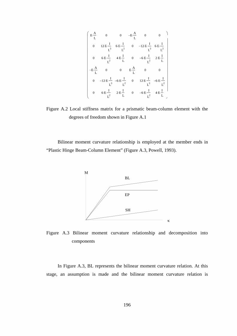
196
Figure A.2 Local stiffness matrix for a prismatic beam-column element with the
degrees of freedom shown in Figure A.1
Bilinear moment curvature relationship is employed at the member ends in
“Plastic Hinge Beam-Column Element” (Figure A.3, Powell, 1993).
Figure A.3 Bilinear moment curvature relationship and decomposition into
components
In Figure A.3, BL represents the bilinear moment curvature relation. At this
stage, an assumption is made and the bilinear moment curvature relation is
EAL
⋅
0
0
E−AL
⋅
0
0
0
12 E⋅I
L3⋅
6 E⋅I
L2⋅
0
12− E⋅I
L3⋅
6 E⋅I
L2⋅
0
6 E⋅I
L2⋅
4 E⋅IL
⋅
0
6− E⋅I
L2⋅
2 E⋅IL
⋅
E−AL
⋅
0
0
EAL
⋅
0
0
0
12− E⋅I
L3⋅
6− E⋅I
L2⋅
0
12 E⋅I
L3⋅
6− E⋅I
L2⋅
0
6 E⋅I
L2⋅
2 E⋅IL
⋅
0
6− E⋅I
L2⋅
4 E⋅IL
⋅
⎛⎜⎜⎜⎜⎜⎜⎜⎜⎜⎜⎜⎜⎜⎜⎜⎝
⎞⎟⎟⎟⎟⎟⎟⎟⎟⎟⎟⎟⎟⎟⎟⎟⎠
M
κ
EP
SH
BL
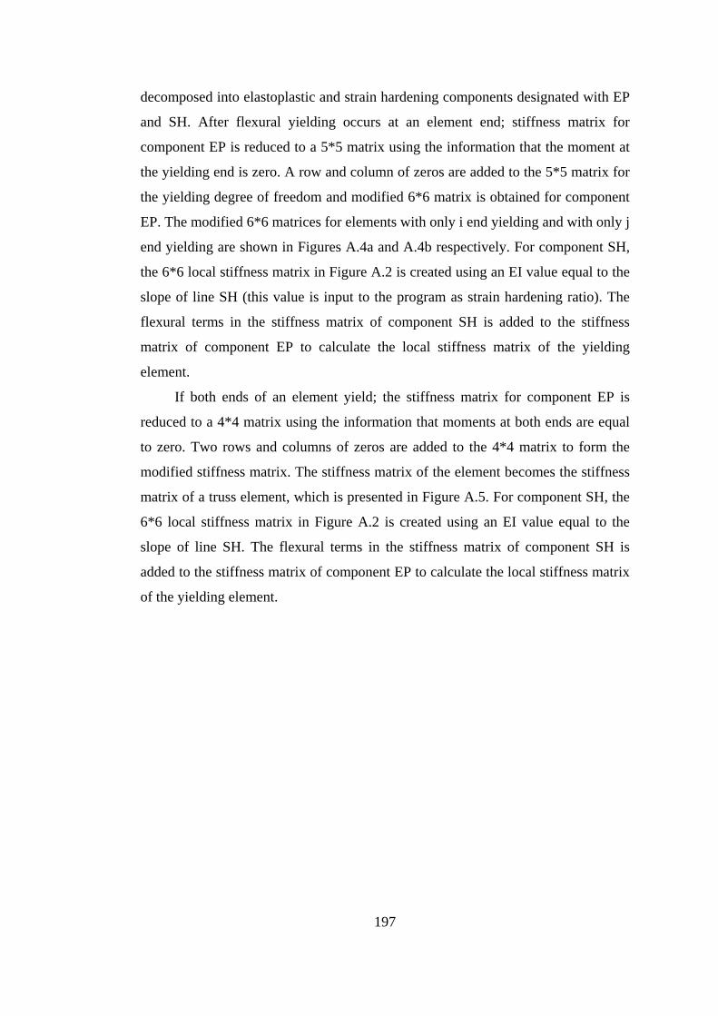
197
decomposed into elastoplastic and strain hardening components designated with EP
and SH. After flexural yielding occurs at an element end; stiffness matrix for
component EP is reduced to a 5*5 matrix using the information that the moment at
the yielding end is zero. A row and column of zeros are added to the 5*5 matrix for
the yielding degree of freedom and modified 6*6 matrix is obtained for component
EP. The modified 6*6 matrices for elements with only i end yielding and with only j
end yielding are shown in Figures A.4a and A.4b respectively. For component SH,
the 6*6 local stiffness matrix in Figure A.2 is created using an EI value equal to the
slope of line SH (this value is input to the program as strain hardening ratio). The
flexural terms in the stiffness matrix of component SH is added to the stiffness
matrix of component EP to calculate the local stiffness matrix of the yielding
element.
If both ends of an element yield; the stiffness matrix for component EP is
reduced to a 4*4 matrix using the information that moments at both ends are equal
to zero. Two rows and columns of zeros are added to the 4*4 matrix to form the
modified stiffness matrix. The stiffness matrix of the element becomes the stiffness
matrix of a truss element, which is presented in Figure A.5. For component SH, the
6*6 local stiffness matrix in Figure A.2 is created using an EI value equal to the
slope of line SH. The flexural terms in the stiffness matrix of component SH is
added to the stiffness matrix of component EP to calculate the local stiffness matrix
of the yielding element.

198
Figure A.4 Stiffness matrices for component EP of a “Plastic Hinge Beam-Column
Element” for which yielding occurs a) at end i, b) at end j
Figure A.5 Stiffness matrix for component EP of a “Plastic Hinge Beam-Column
Element” both ends of which yield
a) b)
EAL
⋅
0
0
E−AL
⋅
0
0
0
3 E⋅I
L3⋅
0
0
3− E⋅I
L3⋅
3 E⋅I
L2⋅
0
0
0
0
0
0
E−AL
⋅
0
0
EAL
⋅
0
0
0
3− E⋅I
L3⋅
0
0
3 E⋅I
L3⋅
3− E⋅I
L2⋅
0
3 E⋅I
L2⋅
0
0
3− E⋅I
L2⋅
3 E⋅IL
⋅
⎛⎜⎜⎜⎜⎜⎜⎜⎜⎜⎜⎜⎜⎜⎜⎝
⎞⎟⎟⎟⎟⎟⎟⎟⎟⎟⎟⎟⎟⎟⎟⎠
EAL
⋅
0
0
E−AL
⋅
0
0
0
3 E⋅I
L3⋅
3 E⋅I
L2⋅
0
3− E⋅I
L3⋅
0
0
3 E⋅I
L2⋅
3 E⋅IL
⋅
0
3− E⋅I
L2⋅
0
E−AL
⋅
0
0
EAL
⋅
0
0
0
3− E⋅I
L3⋅
3− E⋅I
L2⋅
0
3 E⋅I
L3⋅
0
0
0
0
0
0
0
⎛⎜⎜⎜⎜⎜⎜⎜⎜⎜⎜⎜⎜⎜⎜⎝
⎞⎟⎟⎟⎟⎟⎟⎟⎟⎟⎟⎟⎟⎟⎟⎠
EAL
⋅
0
0
E−AL
⋅
0
0
0
0
0
0
0
0
0
0
0
0
0
0
E−AL
⋅
0
0
EAL
⋅
0
0
0
0
0
0
0
0
0
0
0
0
0
0
⎛⎜⎜⎜⎜⎜⎜⎜⎜⎜⎝
⎞⎟⎟⎟⎟⎟⎟⎟⎟⎟⎠

199
CURRICULUM VITAE
PERSONAL INFORMATION Name : Mehmet Selim GÜNAY
Birth Date : 03/10/1978
Birth Place : Ankara / TURKEY
Citizenship : Republic of Turkey
Phone : +90 (312) 2105408
Fax : +90 (312) 2101193
e-mail : [email protected]
EDUCATION 2003 - 2008 Ph.D., Civil Engineering, METU (CGPA: 4.00/4.00)
2000 - 2003 MS, Civil Engineering, METU (CGPA: 3.64/4.00)
1996 - 2000 BS, Civil Engineering, METU (CGPA: 3.60/4.00)
1989 - 1996 Ankara Atatürk Anatolian High School
EMPLOYMENT RECORD 2001 - 2008: Research Assistant, Graduate School of Natural and Applied Sciences,
Pro-Ad Program, METU
COMPUTER SKILLS Computer Programming Languages
MATLAB, Mathcad, Fortran, Visual Basic Software Related to Earthquake Engineering and Structural Analysis
SAP2000, OpenSees, Drain-2DX, SeismoStruct, SeismoSignal, Bispec, NONLIN
200
Other Software
Microsoft Office Applications, AutoCAD SCIENTIFIC PUBLICATIONS International Refereed Journals 1. Sucuoğlu H., Gür T., and Günay M.S., 2004, ‘Performance Based Seismic
Rehabilitation of Damaged R/C Buildings’, Journal of Structural Engineering, Volume 130, No. 10, pp. 1475-1486.
Chapter in a Book 1. Günay M.S., Sucuoğlu H., 2005, ‘An Equivalent Linearization Procedure for
Displacement-Based Seismic Assessment of Vulnerable RC Buildings’, Advances in Earthquake Engineering for Urban Risk Reduction, Editors G. Özcebe, and S.T. Wasti, Kluwer.
International Conference Proceedings 1. Günay M.S., Sucuoğlu H., 2003, ‘Simplified Procedures For Seismic
Assessment of Medium Rise Reinforced Concrete Building Structures’, Concrete Structures in Seismic Regions, FIB Symposium, 6-9 May, Athens, Greece, Paper No: 79.
2. Günay M.S., Sucuoğlu H., 2004, ‘A Comparative Evaluation of Performance-
Based Seismic Assessment Procedures’, 13th World Conference on Earthquake Engineering, 1-6 August, Vancouver, Canada, Paper No: 0453.
3. Günay M.S., Sucuoğlu H., 2005, ‘Capacity-Based Equivalent Linear Modeling
of the SPEAR Test Frame’, SPEAR International Workshop, Ispra, Italy. 4. Günay M.S., Sucuoğlu H., 2006, ‘Capacity Control Method For Seismic
Assessment of Low-to-Medium Rise Reinforced Concrete Buildings’, First European Conference on Earthquake Engineering and Seismology, 3-8 September, Geneva, Switzerland, Paper No: 1042.
National Conference Proceedings 1. Sucuoğlu H., Günay M.S., 2003, ‘Orta Yükseklikteki Betonarme Yapılar için
Basitleştirilmiş Deprem Dayanımı Değerlendirme Yöntemleri’, Beşinci Ulusal Deprem Mühendisliği Konferansı, İstanbul, Türkiye.
Recommended