An Enhanced Oil Recovery Micromodel Study with Associative and
Conventional Polymers
Diploma Thesis
Markus Buchgraber
Submitted to the
Department of Petroleum Engineering
University of Leoben, Austria
September 2008

I declare in lieu of oath, that I wrote this thesis and performed the associated research myself, using only literature cited in this volume.
Markus BUCHGRABER
Leoben, October 2008

Acknowledgements
I would like to thank my advisors, Prof. Anthony Kovscek and Dr. Louis Castanier, for
their assistance and guidance in research and for their remarkable support in case of
experimental difficulties. I also gratefully acknowledge the support of all the members
and Industrial Affiliates of the Stanford Petroleum Research Institute (SUPRI-A).
Furthermore, I would like to thank Dr. Clemens Torsten for all the preparation work
and organization and his indispensable phone calls, which gave me new inspiration
and motivation for this work.
I also would like to thank Prof. Leonhard Ganzer for his advice and support during my
master thesis in Stanford and Leoben.
I am very grateful to OMV for giving me this great and unique opportunity and financial
support to pursue my master thesis at Stanford University.
Also special thanks to SNF Floerger for providing the polymers and information.
Finally, I want to thank my family for their incredible support during my semesters
abroad. Your help, patience and love made it a lot easier to do my research and finish
my studies. Mom, Dad, Christian and my dear Verena, thanks for being with me in
good as well as in hard times!

Table of Contents
Acknowledgements ......................................................................................................3 Table of Contents ..........................................................................................................4 List of Figures................................................................................................................6 List of Tables................................................................................................................11 Abstract ........................................................................................................................12 Kurzfassung.................................................................................................................14 Introduction..................................................................................................................16
Viscous Fingering..........................................................................................................................................19 Polymer Flooding Mechanism...................................................................................21 Screening of an EOR Polymer Flooding Project.....................................................26 Development and Evaluation of a Polymer Flooding Project................................29 Chemistry of EOR Polymers ......................................................................................34
Polysaccharide..............................................................................................................................................34 Xanthan..............................................................................................................................................................................35
Synthetic Polymers .......................................................................................................................................36 Polyacrylamide ..................................................................................................................................................................36 Associative Polymer..........................................................................................................................................................38
Polymer Degradation Mechanism................................................................................................................39 Rheological Behaviour of Polymers .........................................................................42
Viscosity.........................................................................................................................................................42 Newtonian Fluids...............................................................................................................................................................43 Non-Newtonian Fluids.......................................................................................................................................................43
Experimental Apparatus.............................................................................................45 Injection System............................................................................................................................................45 Data Gathering Equipment ...........................................................................................................................46
Micromodel...................................................................................................................48 Micromodel Fabrication.................................................................................................................................50 Micromodel Holder........................................................................................................................................57
Experimental Procedure.............................................................................................59 Permeability Measurement...............................................................................................................................................62
Image Analysis ............................................................................................................72 Image Analyse in G.I.M.P.............................................................................................................................74 Image Analysis in MATLAB..........................................................................................................................76
Sensitivity Analysis of RGB Values..................................................................................................................................78 Meso Scale Image Analysis .........................................................................................................................81
Brine Mixing .................................................................................................................83 Polymer Mixing ............................................................................................................84 Viscosity Measurement Experiments .......................................................................86 Shear Rate Experiment...............................................................................................90 Relative Permeabilities ...............................................................................................92 Permeability Reduction ..............................................................................................97

Polymer Adsorption.....................................................................................................................................101 Oil ................................................................................................................................103 Problems ....................................................................................................................105 Experimental Results and Discussions .................................................................108
Brine Flood ..................................................................................................................................................109 Associative Polymer Floods........................................................................................................................111 Conventional Polymer Floods.....................................................................................................................119 Combination Flood Experiment ..................................................................................................................132 Residual Oil Recovery Experiment.............................................................................................................135
Conclusions ...............................................................................................................136 Follow up......................................................................................................................................................................... 138
References .................................................................................................................139 Nomenclature.............................................................................................................142 Appendix ....................................................................................................................143
Appendix A ..................................................................................................................................................143 Appendix B ..................................................................................................................................................147 Appendix C..................................................................................................................................................149

List of Figures
Figure 1: Five spot displacement pattern: stable and unstable displacement ...............17
Figure 2: Development of viscous fingers according to van Meurs................................19
Figure 3: Typical relative permeabilities for oil and water of a water wet sandstone and fractional flow curves for displacement of oil by water and polymer solution (Viscosities oil: 15 cp; water: 1 cp; polymer solution: 15cp) [8] ........23
Figure 4: Mobility ratio for the displacement of oil by water and polymer solution as a function of the saturation of the displacing phase[8]. ..................................23
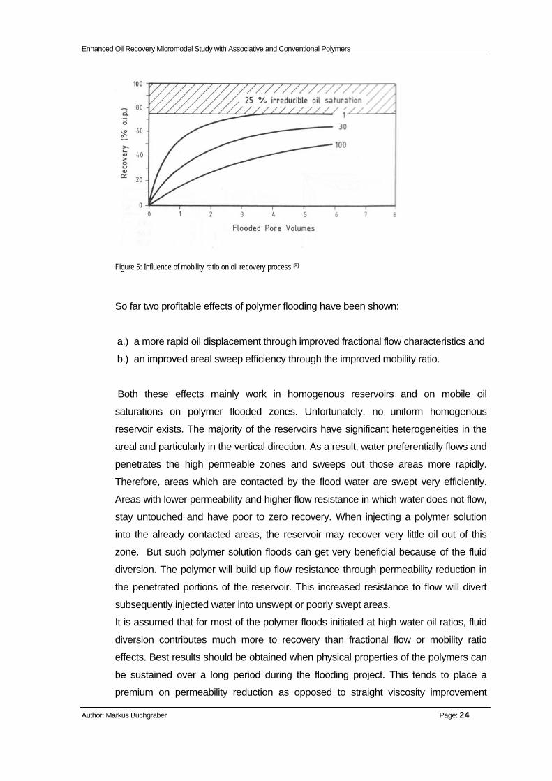
Figure 5: Influence of mobility ratio on oil recovery process [8] .......................................24
Figure 6: Possible effect of polymer solution when dealing with a heterogeneous reservoir [8] ......................................................................................................25
Figure 7: Staged process for polymer flood project evaluation and development [10]....32
Figure 8: Representative Portion of polymer flood project evaluation and development matrix [10] ...................................................................................33
Figure 9: Molecular structure of hydroxyethyl cellulose [8]...............................................34
Figure 10: Molecular structure of xanthan[8] ....................................................................36
Figure 11: Structure of polyacrylamide (not hydrolized) [8]..............................................36
Figure 12: Molecular structure of partially hydrolysed polyacrylamid[8] ..........................37
Figure 13: Flow curves of a 1000 ppm polyacrylamide solution at different hardness of mixing water: 1.) 1.6°dH; 2.) 5°dH; 3.) 15°dH; 4.) 25°dH. (1°dH � 10 mg CaO/l) [8] ................................................................................40
Figure 14: Influence of salinity on viscosity .....................................................................41
Figure 15: Schematic picture of two planes moving in the same direction for shear rate calculation ...............................................................................................42
Figure 16: Characteristic rheological behaviour of Newtonian fluids[15]..........................43
Figure 17: Shear rate determines viscosity in pseudoplastic fluids [15] ...........................44
Figure 18: Shear thicking viscosity graphs [15] .................................................................44
Figure 19: Teledyne Isco Model 100 DM syringe pump.................................................46
Figure 20: Vessel system with decane and brine for water............................................46
Figure 21: Brookfield viscometer with example beaker and spindle for measurements................................................................................................47
Figure 22: Nikkon Eclipse microscope ............................................................................47

Figure 23: SEM image of a thin section of a Berea Sandstone [25].................................50
Figure 24: Unit cell of the micromodel [17] ........................................................................51
Figure 25: Repeating units of the micromodel[17].............................................................51
Figure 26: Schematic picture of the micromodel with inlet and outlet fracture and ports [17] ...........................................................................................................52
Figure 27: Micromodel fabrication: a) Coating with photoresist; b) Exposing and developing; c) Etching; d) Bonding................................................................53
Figure 28: Lithography mask, coated with chrome.........................................................54
Figure 29: SEM image of etched micromodel. Pore diameters between 10 μm -150 μm [25] ..............................................................................................................56
Figure 30: Bonded micromodel [16]...................................................................................57
Figure 31: Micromodel holder sketch ..............................................................................58
Figure 32: Micromodel with O-rings graving....................................................................58
Figure 33: Micromodel holder with fixed micromodel .....................................................58
Figure 34: O-ring graving without and with o-ring ...........................................................58
Figure 35: Experimental setup for brine saturation .........................................................61
Figure 36: Brine saturated micromodel with trapped CO2 (white bubbles) ...................61
Figure 37: Schematic view of permeability measurement with a bubble flow meter.....62
Figure 38: Setup for oil saturation with water pump and oil vessel ................................64
Figure 39: Well oil saturated micromodel (brown: oil; white: grains and water).............65
Figure 40: Poor oil saturated micromodel .......................................................................65
Figure 41: Oil saturation in relation to time......................................................................65
Figure 42: Meso scale oil saturation after time (from the left top to the right bottom: a,b,c,d,e,f).......................................................................................................67
Figure 43: Micro scale oil saturation after time................................................................68
Figure 44: Micromodel reverse side after oil saturation with a leaking O-ring ...............68
Figure 45: Inlet fractures from different experiments with different stages of clearness. From top to bottom decreasing clearness...................................69
Figure 46: Polymer flooding set up with water pump and polymer vessel.....................70
Figure 47: Micro scale pictures at the displacing front after different time intervals (5 sec: 10 sec; 15sec; 20 sec).......................................................................71
Figure 48: Micromodel grid for taking micro scale photographs.....................................73
Figure 49: Saturated micromodel ready for a polymer flood ..........................................73
Figure 50: Typical micromodel histogram of a micro scale picture. Three humps represent oil, polymer or water saturation, grain edges and grains from the left to the right...........................................................................................75
Figure 51: Histogram with threshold limit (blue area) .....................................................75
Figure 52: Histogram after setting a threshold value and converting into a binary picture. The bars at the beginning and the end of the diagram represent the frequency of black and white. ..................................................................75
Figure 53: Processed binary image of Figure 49............................................................76
Figure 54: Only coated and exposed micromodel (not etched) .....................................77
Figure 55: Etched empty micromodel..............................................................................77
Figure 56: 100% water saturated micromodel ................................................................78
Figure 57: Pore edges after digital processing................................................................78
Figure 58: Modified binary image from the base case....................................................79
Figure 59: Modified picture with the largest deviation from the base case ....................79
Figure 60: Polymer injection set up with camera, lights and diffusion box.....................81
Figure 61: Unprocessed meso scale photo.....................................................................82
Figure 62: Manually marked swept area (black) .............................................................82
Figure 63: Digitally converted binary image ....................................................................82
Figure 64: Ohaus digital scale .........................................................................................83
Figure 65: Stirrer with beaker and stirring bone ..............................................................83
Figure 66: Table 6: Chemical composition for brine mixing[26]........................................83
Figure 67: Polymer sample beakers................................................................................85
Figure 68: Cartridge filter with 15 microns average filter size.........................................85
Figure 69: Cartridge filter holder ......................................................................................85
Figure 70: Associative polymer solution viscosity measurement ...................................87
Figure 71: Conventional polymer solution viscosity measurement ................................87
Figure 72: Viscosity measurements for associative polymer solution from Alberta research council [26] ........................................................................................88
Figure 73: Viscosity measurement before and after filtering with a cartridge filter ........89

Figure 74: Oil saturation at relative permeability measurement .....................................93
Figure 75: Oil saturation when measuring water relative permeability...........................93
Figure 76: Relative permeability curves of oil and water according to the measurements................................................................................................94
Figure 77: Influence of mobility ratio on breakthrough time and sweep efficiency ........95
Figure 78: Polymer plugged (red) areas near inlet fracture of the micromodel .............99
Figure 79: Dyed polymer solution with food colour .........................................................99
Figure 80: Viscosity measurements before and after flooding the polymer solution through the micromodel .............................................................................. 101
Figure 81: Oil viscosity measurements at room temperature (22.4°C)....................... 103
Figure 82: Oil viscosity measurements at reservoir temperature (30.0°C) ................. 104
Figure 83: Brine flood meso scale series till breakthrough and till ultimate recovery BT-time: 71 min. .......................................................................................... 110
Figure 84: Associative polymer flood S255, 500 ppm; BT-time: 51 min. .................... 113
Figure 85: Associative polymer flood S255, 750 ppm; BT-time: 50 min. .................... 114
Figure 86: Associative polymer flood S255, 1000 ppm; BT-time: 91 min. .................. 115
Figure 87: Associative polymer flood S255, 1250 ppm; BT-time: 107 min. ................ 116
Figure 88: Associative polymer flood S255, 1500 ppm; BT-time: 64 min. .................. 117
Figure 89: Associative polymer flood S255, 2500 ppm; BT-time: 213 min. ................ 118
Figure 90: Conventional polymer flood FP3630, 500 ppm; BT-time: 25 min.............. 120
Figure 91: Conventional polymer flood FP3630, 750 ppm; BT-time: 81 min.............. 121
Figure 92:Conventional polymer flood FP3630, 1000 ppm; BT-time: 17 min............. 122
Figure 93: Conventional polymer flood FP3630, 1250 ppm; BT-time: 28 min............ 123
Figure 94: Conventional polymer flood FP3630, 1500 ppm; BT-time: 25 min............ 124
Figure 95: Meso scale photograph at breakthrough with finger base line and counted fingers............................................................................................ 126
Figure 96: Effect of increasing concentration on finger number for conventional polymer ........................................................................................................ 127
Figure 97: Dependency of finger length on polymer concentration for conventional polymer ........................................................................................................ 127
Figure 98: Effect of increasing concentration on finger number for associative polymer ........................................................................................................ 128
Figure 99: Dependency of finger length on polymer concentration for associative polymer ........................................................................................................ 128
Figure 100: Swept areas for conventional and associative polymer solution ............. 129
Figure 101: Processed binary images of associative polymer for swept area calculation. From top to bottom: 500 ppm, 750 ppm, 1000 ppm, 1250 ppm, 1500 ppm, 2500 ppm......................................................................... 130
Figure 102: Processed binary images of conventional polymer for swept area calculation. From top to bottom: 500 ppm, 750 ppm, 1000 ppm, 1250 ppm, 1500 ppm ........................................................................................... 131
Figure 103: Combination flood. Switch from brine injection to polymer solution at picture 5 (third row second picture) ............................................................ 134
Figure 104: Photoresist Coater[30] ................................................................................. 144
Figure 105: Developing machine-chemical Wash[30].................................................... 145
Figure 106: STS-Etching machine with control computer[30]........................................ 145
Figure 107: Zygo-electron microscope[30] ..................................................................... 146

Enhanced Oil Recovery Micromodel Study with Associative and Conventional Polymers
Author: Markus Buchgraber Page: 11
List of Tables
Table 1: Optical properties of microscope lenses [16] ......................................................46
Table 2: Permeability measurements with constant pressure .......................................63
Table 3: Permeability measurements with constant flow rate........................................63
Table 4: Permeability measurement with bubble flow meter..........................................63
Table 5: RGB-Sensitivity analysis ...................................................................................80
Table 6: Technical dates for used polymers [27] ..............................................................85
Table 7: Pressure recordings during polymer flooding in a water saturated micromodel ......................................................................................................90
Table 8: Input data for viscosity calculation.....................................................................90
Table 9: Input data for shear rate calculation..................................................................91
Table 10: Results for different fluid coefficients, npl.........................................................91
Table 11: Input data for water relative permeability curve calculation ...........................94
Table 12: Input data for oil relative permeability curve calculatio...................................94
Table 13: Mobility ratios for associative polymer solution and crude oil (450 cp)..........96
Table 14: Permeability measurements before injecting the polymer solution (measured with const. flow rate) ...................................................................100
Table 15: Permeability measurement after injecting the polymer solution (measured with const. flow rate) ...................................................................100
Table 16: Results for brine- and associative polymer flood experiments ....................125
Table 17: : Results for brine- and conventional polymer flood experiments................125
Enhanced Oil Recovery Micromodel Study with Associative and Conventional Polymers
Author: Markus Buchgraber Page: 12
Abstract
Half of the recovery of the worldwide oil production is due to waterflooding projects. Mainly lighter
oils with lower in situ viscosities are recovered by water flooding. Buckley-Leverett and Darcy´s
Law can describe the displacement process of these stable displacements very well. Higher
viscous oils suffer from unfavourable mobility ratios and, therefore, show unstable displacement.
Viscous fingers cause an early breakthrough leaving a lot of bypassed oil behind them and having
high watercuts early in their flooding life. This behaviour can hardly be described by the Buckley
Leverett equation and does not predict reservoir performance very accurately.
By adding polymer into the injection water and, therefore, increasing the viscosity, the
displacement process will have a more favourable mobility ratio and hence a more stable
displacement. In addition, the effect of the plugging of high permeability paths so that bypassed
areas get in contact with the displacement fluid, is desired.
Polymer flooding has been done for almost 40 years with hydrolysed polyacrylamide or xanthan,
which are referred to as conventional polymers. A new type of polymer, a so-called associative
polymer, has been developed recently. It has a greater resistance against salinity and at the same
concentration a higher viscosity than conventional polymers, which would reduce the costs of a
polymer flooding project significantly.
The purpose of this study is to improve the understanding of the immiscible displacement of
conventional and associative polymer solutions with dead oil (450 cP). Forced imbibitions
experiments were conducted to observe front stability, breakthrough-time and recovery and
ultimate recovery for different polymer concentrations and polymers.
Experiments were conducted in a micromodel which had geometrically and topologically the same
homogenous pore space as Berea sandstone. It acts as an artificial reservoir and is an etched
silicon wafer bonded with glass to build the flow channels. The main advantage compared to
conventional core experiments is that the displacement process can be observed at meso and
micro scale with a microscope without any CT-scanning tools. Records in form of high resolution
photographs and videos describe the displacement process at micro and meso scale.
Initial water saturation, water saturation at breakthrough, swept area at breakthrough and ultimate
recovery are determined and calculated with digital analyses. Additional data recorded before and

Enhanced Oil Recovery Micromodel Study with Associative and Conventional Polymers
Author: Markus Buchgraber Page: 13
during experiments are oil and polymer viscosity, mobility ratios, shear rates for polymer solution in
the micromodel, absolute and relative permeabilities, injection rate and pump pressure.
Analyses stated that with increasing polymer concentration recovery, sweep efficiency and front
stability also improved. Associative polymer solutions did not convince significantly in terms of
recovery but showed better front stabilities than conventional polymer solutions. For this set of
experiments best results were obtained with polymer concentrations of 1250 ppm to 1500 ppm. It
was also shown that there exists a upper limit for polymer concentration. Exceeding this led to a
pore plugging effect and poor recovery.

Enhanced Oil Recovery Micromodel Study with Associative and Conventional Polymers
Author: Markus Buchgraber Page: 14
Kurzfassung
Die Hälfte des weltweit geförderten Erdöls wird mit Hilfe von Wasserfluten gewonnen.
Hauptsächlich werden dabei Erdölfelder mit leichtem Öl und niedriger Viskosität gefördert. Um
diese Prozesse mathematisch zu beschreiben, können die Gleichungen von Buckley und Leverett
und das Gesetz von Darcy verwendet werden.
Höher viskoses, schweres Öl hat mit Hilfe von Wasserfluten sehr schlechte Erfolgsergebnisse.
Grund dafür sind unvorteilhafte Mobilitätsverhältnisse, die zu einem nicht stabilem
Verdrängungsprozess führen. Viskose Finger bilden sich und führen zu einem Durchbruch der
Wasserfront. Hohe verfrühte Wasserproduktionen und nicht kontaktierte Reservoirgebiete mit
hohen Ölsättigungen sind die Folge.
Das Beimischen von kleinen Mengen von Polymeren kann die Viskosität des Injektionswassers
signifikant erhöhen und zu besseren Mobilitätsverhältnissen, die stabilere
Verdrängungsverhältnisse haben, führen. Zusätzlich werden Kanäle erhöhter Permeabilität
verstopft und das Flutwasser so zu nicht kontaktierten Bereichen geleitet.
Der Prozess des Polymerfluten wird seit mehr als 40 Jahren kommerziell eingesetzt. Die am
häufigsten verwendeten Polymere sind hydrolisierte Polyacrylamide und Xanthan. Sie werden als
konventionelle Polymere bezeichnet.
Seit kurzem wurde ein sogenanntes assoziatives Polymer getestet. Durch funktionelle Gruppen
besitzt es eine höhere Resistenz gegen Salinität und kann bei gleicher Konzentration höhere
Viskositäten als konventionelle Polymere haben.
Das Ziel dieser Studie war es das Verständnis von unmischbaren Verdrängungsvorgängen von
konventionellen und assoziativen Polymer-Lösungen mit mittelschweren Ölen (250cp) zu
verbessern. Forced Imbibtion Experimente mit verschiedenen Polymer Konzentrationen wurden
durchgeführt um Frontstabilität, Durchbruchszeit -und Entölung und Endentölung zu bestimmen
und zu beobachten. Als poröses Medium dienten Micromodels, welche die gleichen
geometrischen und topologischen homogenen Porenstrukturen von Berea Sandstein aufweisen.
Eine geätzte Silkonscheibe, die durch eine Glasplatte abgedeckt und verklebt wird, bildet den
künstlichen Kern mit den nachgeahmten Porenkanälen. Vorteil dieser Technik ist, dass der
Verdrängungsvorgang visuell im Micro- als auch im Mesobereich mit Hilfe eines Mikroskops
beobachtet werden kann und kein Röntgengerät verwendet werden muss.

Enhanced Oil Recovery Micromodel Study with Associative and Conventional Polymers
Author: Markus Buchgraber Page: 15
Hochaufgelöste Photographien im Micro- und Mesobereich beschreiben anfängliche
Wassersättigung, Wassersättigungen zur Front Durchbruchszeit, Endentölung und geflutete
Bereiche. Zusätzliche Daten, die vor und während der Experimente aufgenommen wurden wie
absolute und relative Permeabilität, Viskositäten des Öls und der Polymer Lösungen,
Mobilitätsverhältnisse, Scheer Raten und Injektionsraten sowie dazugehörige Pumpendrücke
sollen für ein besseres Verständnis der Flutversuche sorgen.
Auswertungen ergaben dass mit erhöhten Polymer Konzentrationen, Entölungsgrad, geflutete
Bereiche und Frontstabilitäten auch entscheidend gesteigert werden konnten. Assoziative
Polymerlösungen ergaben keine besseren Entölungen als konventionelle Polymerlösungen,
führten aber zu stabileren Fronten. Beste Ergebnisse für diese Experimentreihe ergaben
Polymerkonzentrationen mit 1250ppm bis 1500ppm. Zusätzlich konnte gezeigt werden, dass es
eine kritische Polymerkonzentration gibt. Experimente mit höheren Konzentrationen führten zu
Porenverstopfungen und schlechten Entölungen.

Enhanced Oil Recovery Micromodel Study with Associative and Conventional Polymers
Author: Markus Buchgraber Page: 16
Introduction
Primary oil production relies on the natural energy present in a hydrocarbon bearing
zone. The main energy sources are water and gas, which displace the oil to the
production wells. Most often this process contributes to only a minor part of the
production of the original oil in place. Thus, different supplemental recovery
techniques have been developed and invented through the last decades to increase
the recovery for reservoirs.
Volumetric sweep efficiency and microscopic displacement efficiency determine the
viability of a displacement process in an oil reservoir. Enhanced oil recovery (EOR)
usually utilizes the injection of different fluids into the reservoir. The injected fluids
supplement the displacement process with natural energy in the reservoir. Chemical
flooding (alkaline flooding or micellar polymer flooding), miscible displacement (carbon
dioxide or hydrocarbon injection), and thermal recovery (steamflood or in-situ
combustion) are the three major types of enhanced oil recovery. The selection of one
of those specific techniques depend on reservoir temperature, pressure, depth, net
pay, permeability, residual oil and water saturation, porosity and fluid properties, such
as oil API gravity and viscosity.[1]
Mobility control and chemical processes are the main processes involved in enhanced
oil recovery techniques. Polymer flooding utilizes the mobility control process. A
polymer flood application is designed to develop a favourable mobility ratio between
the injected polymer solution and the oil bank being displaced ahead of the polymer
solution slug. The main target is to produce a uniform displacement in vertical and
horizontal direction to avoid viscous water fingers, which take the shortest path to the
production well. Figure 1 represents a desired displacement process during a polymer
flood and an undesired case, where viscous fingers cause an early breakthrough in a
water flood project. During the last decades, the molecular weight and quality of
polymers have improved their flood efficiency and success rate significantly.
Therefore, the interest in users, manufactures and research facilities has significantly
increased. Rheological properties and the behaviour by displacing heavy and
intermediate viscous oils are the target of current investigations. As a rule of thumb,
polymer flood applications were applied for oils with viscosities less than 100
centipoises (cp). Nowadays oil viscosities up to 2000 cp have been tested with

Enhanced Oil Recovery Micromodel Study with Associative and Conventional Polymers
Author: Markus Buchgraber Page: 17
polymer solutions. A reason for that is the increased oil price, which broads the
sometimes risky application of enhanced oil recovery techniques. In addition, the
advent of new technology, combining two technologies like horizontal wells and
polymer flooding, can make the initiation of a polymer flood quite economically and
technically successful.
Figure 1: Five spot displacement pattern: stable and unstable displacement
A polymer flood project requires more technical equipment and knowledge compared
to conventional water floods. A number of polymer projects have been implemented
since the 1960's. However, the mobility control process alone does not employ the
microscopic displacement efficiency and suffers from a low recovery efficiency, thus
the incremental oil recovery is limited, usually under 10% of the original oil in place
(OOIP). Analyzed statistical data from the DOE of the field wide projects showed that
the median recovery of oil was 2.91% OOIP[2].
This study investigates the behaviour of so-called associative polymers, which have
special functional groups which provide a better viscosity than conventional polymers
of the same concentration. Additionally, they are suitable for mixing with very high
saline reservoir brines. Different concentrations of conventional and associative
polymers solutions were tested to understand the relationship of polymer
concentration with sweep efficiency and recovery. Polymer solution can also be used
with surfactants and alkali agents. For the purpose of this work, only polymer solution
mixed with brine is used to observe and understand the flow mechanism. Instead of a
real core, micromodels act as an artificial core. An etched silicon wafer bonded with a

Enhanced Oil Recovery Micromodel Study with Associative and Conventional Polymers
Author: Markus Buchgraber Page: 18
pyrex glass represents the pore structure of a Berea sandstone and provides artificial
flow channels. High resolution photographs on micro and meso scale are used to
describe flow behaviour and pattern and to determine recovery and sweep efficiency.
As a baseline, a water flood experiments was conducted. Additionally, the influence of
a late start of a polymer injection after breakthrough has been tested and evaluated.
Also, the possible recovery of residual oil with a polymer solution has been tested.
Rheological experiments with oil and augmented polymers give a better
understanding of shear rate and viscosity behaviour during the experiments.
The first chapters will give an overview about polymer flooding including the
advantages, screening criteria and field development and evaluation processes for a
polymer flood. Next chapters will deal with the chemical and rheological properties of
polymer solutions. Followed by this, the experimental apparatus and the experimental
procedure including are described in more detail. The final part presents the results
and a follow up.

Enhanced Oil Recovery Micromodel Study with Associative and Conventional Polymers
Author: Markus Buchgraber Page: 19
Viscous Fingering Buckley and Leverett´s displacing theory assumes that water displaces oil as a
smooth and substantially straight interface. Viscous fingers which developed in
displacement experiments disproved Buckley and Leverett´s theory. In general
viscous fingers refer to the onset and evolution of instabilities that evolve in the
displacement of fluids in a porous system. Most often instabilities are intimately linked
to viscosity variations between phases. Viscous structures typically consist of fingers
invading into the displaced fluid and propagating through the porous medium and
leaving clusters of the displaced fluid behind. Once the path of displacing fluid has
broken through and flows into the production well, the production well will henceforth
preferentially produce the displacing fluid, which flows more easily because of the
lower viscosity and better fractional flow characteristic. Viscous fingers depend on
viscosity ratios, relative permeability curves, initial water saturation and flow rates of
injected fluid.
One of the first experiments, which showed the viscous displacement process of water
by oil was made by van Meurs[3] [4] . Fine powdered glass served as a porous medium.
He came up with the conclusion that a water drive at favourable viscosity ratios is
efficient, but the presence of stratified layers with different permeabilities can reduce
its success significantly. Furthermore, he stated that unfavourable viscosity ratios lead
to poor sweep efficiency and the influence of stratification was minor. A displacement
of viscosity ratio of a unity led to a stable displacement. He was able to visualize the
viscous fingers depending on injected fluid, Wi, as can be seen in Fig. 2.
Figure 2: Development of viscous fingers according to van Meurs.

Enhanced Oil Recovery Micromodel Study with Associative and Conventional Polymers
Author: Markus Buchgraber Page: 20
In 1963, Benham and Olsen studied the behaviour of viscous fingers in an open and
packed Hele-Shaw model (1 ft x 4 ft). Flow velocities of 0.06 to 0.2 ft/hour and mobility
ratios from 1 to 9.3 were used for the displacement experiments. Results indicated
that the length of viscous fingers increased linearly with increasing mobility ratio and
increasing flow rate. They were not able to determine the initiation point of a viscous
finger but they observed that fingers decreased towards the end of the model due to
microscopic dispersion or diffusion effects[5].
Saffman and Taylor[6] used a Hele-Shaw model to demonstrate the instability
problems. A less viscous fluid was injected into a more viscous one constrained
between two parallel thin glass plates. Wave-like projections, known today as viscous
fingers, exhibited the resulting interface between the fluids. They investigated that on
the one hand surface tension served to stabilize the system by trying to minimize the
surface, and on the other hand the viscosity difference destabilized the system
promoting the growth of the fingers. Results show that single fingers were produced,
and that unless the flow is very slow λ = (width of finger)/(width of channel) is close to
½ , so that behind the tips of the advancing fingers the widths of the two columns of
fluid were equal.
Other experiments with lower viscous fluids for displacing like air and water stated
that λ is only a function of viscosity, speed of advance and interfacial tension.
Van Meurs and van der Peol [7] conducted linear displacement experiments with oil
and water at unfavourable mobility ratios in a transparent porous medium.
Experimental observations described mathematically and led to accurate expressions
of oil production and pressure drops across the porous media as a function of
cumulative water injection with the oil-water viscosity ratio as a parameter. The
theoretical results were applied to sand filled tubes and to field scale applications.
Both led to satisfying predictions in oil and water production and breakthrough time.

Enhanced Oil Recovery Micromodel Study with Associative and Conventional Polymers
Author: Markus Buchgraber Page: 21
Polymer Flooding Mechanism
By adding small amounts of soluble polymers into water a very viscous aqueous
solution can be obtained. This viscous fluid can reduces mobility ratios in flooding
operations significantly. It was regarded as one of the most successful EOR methods
in the 80s, although by definition polymer flooding projects did not increase the
volumetric sweep efficiency of the reservoir rock. The remaining oil saturation after a
polymer flood is the same as after a water flood. Nevertheless it was observed that
polymer solutions can interact with the rock surface and change wettability to more
water wet characteristics leading to residual oil recovery. Compared to other EOR
methods like chemical floods, which reduce the interfacial tension and therefore
reduce the residual oil saturation, polymer floods cannot produce significant amounts
of residual oil. Polymer flooding does not reduce the residual oil saturation noticeable,
but is rather a way of reaching the residual oil saturation more quickly and allows it to
be reached more economically. Hence, almost the same physical laws used for water
floods can be applied for the injection of the polymer solution.
To make the oil recovery process with polymer solution more efficient there are three
potential ways:
• through the effects of polymers on fractional flow
• by decreasing the water/oil mobility ratio, and
• by diverting injected water from zones that have been swept
Relative permeability relationships and viscosities of oil and water are the main
parameters influencing the way and success of a reservoir approaching its ultimate
residual oil saturation. Those two factors are combined and used in the formulation of
the fractional flow. Assuming that the oil and the water are flowing simultaneously
through a segment of a porous medium, the fractional flow of crude oil, fo, and water,
fw, can be expressed as in Eq. 1. [3]

Enhanced Oil Recovery Micromodel Study with Associative and Conventional Polymers
Author: Markus Buchgraber Page: 22
Any change of the term ,which increases the fractional flow of the oil, will lead to
an improvement of recovery. Polymers, when added to water, have the ability of
increasing the viscosity of water, μw. Another effect is that once they have flooded a
zone, they can reduce the permeability to water, krw. This effect occurs at parts of the
reservoir having high mobile oil saturation, anywhere where the relative permeability to
oil is above zero. But having already very low mobile oil saturation and therefore a low
kro, changes in μw and krw will not result in any significant changes in the fractional flow
of oil. Hence the fractional flow effect is more significant to projects where polymer
flooding has been applied early in a field life when mobile oil saturation is still high. Oil
viscosities also contribute to the fractional flow. Areas of higher oil viscosity will show
greater tendency of water flowing than oil.
As a result the water breakthrough and therefore the water production will be early in
the field life and a lot of mobile bypassed oil will be left in the reservoir. Thus fractional
flow effects show more likely in viscous oil reservoirs. Below characteristic flow curves
are plotted for oil having a viscosity of 15 cp and the displacing fluids water with 1 cp
and a polymer solution having 15 cp. The saturation at the front for the polymer flood
Spf and the water flood Swf and also the saturation at the breakthrough Sbtp and Sbtw are
given in Fig. 3. Both saturations at the front and at breakthrough are distinctly higher
for the polymer flood than for the waterflood. This shows the better performance of a
polymer flood to a water flood. In Fig 4. the corresponding mobility ratios to Fig.3 can
be seen. It is shown that mobility ratios in water floods at low water saturations can be
below 1, whereas for polymer floods at high saturations, the mobility ratio can exceed
1 as well.

Enhanced Oil Recovery Micromodel Study with Associative and Conventional Polymers
Author: Markus Buchgraber Page: 23
Figure 3: Typical relative permeabilities for oil and water of a water wet sandstone and fractional flow curves for displacement of oil by water and polymer solution (Viscosities oil: 15 cp; water: 1 cp; polymer solution: 15cp) [8]
Figure 4: Mobility ratio for the displacement of oil by water and polymer solution as a function of the saturation of the displacing phase[8].
The mobility ratio of a flood is the primary determinant of areal sweep efficiency for a
given well spacing and pattern and is defined for water floods in Eq. 2 as:
No real reservoir can be swept uniformly and even in a homogenous reservoir a 100
% areal sweep at water breakthrough and an economically water/oil ratio cannot be
achieved. For any given reservoir, the recovery till breakthrough will decrease with
increasing mobility ratio. Also, the later recovery will be less for a given volume of
water injected. Polymer solution may improve the mobility ratio in the same way as
mentioned above. They can increase the water viscosity or decrease the water
relative permeability. It must be considered that at low mobile oil saturations there is
only small potential for improvement. From this point of view, a secondary over a
tertiary application for a polymer flood is favourable. Another example of the effect of
different mobility ratios is given below in Fig 5. This figure clearly demonstrates the
improvement in recovery related to a decreasing mobility ratio. The irreducible oil
saturation should be the same for all cases, but the period of time and therefore the
volume injected can vary slightly. The improvement shown below is that the oil can be
recovered earlier at a lower water cut and thus in practice at lower lifting costs.
Enhanced Oil Recovery Micromodel Study with Associative and Conventional Polymers
Author: Markus Buchgraber Page: 24
Figure 5: Influence of mobility ratio on oil recovery process [8]
So far two profitable effects of polymer flooding have been shown:
a.) a more rapid oil displacement through improved fractional flow characteristics and
b.) an improved areal sweep efficiency through the improved mobility ratio.
Both these effects mainly work in homogenous reservoirs and on mobile oil
saturations on polymer flooded zones. Unfortunately, no uniform homogenous
reservoir exists. The majority of the reservoirs have significant heterogeneities in the
areal and particularly in the vertical direction. As a result, water preferentially flows and
penetrates the high permeable zones and sweeps out those areas more rapidly.
Therefore, areas which are contacted by the flood water are swept very efficiently.
Areas with lower permeability and higher flow resistance in which water does not flow,
stay untouched and have poor to zero recovery. When injecting a polymer solution
into the already contacted areas, the reservoir may recover very little oil out of this
zone. But such polymer solution floods can get very beneficial because of the fluid
diversion. The polymer will build up flow resistance through permeability reduction in
the penetrated portions of the reservoir. This increased resistance to flow will divert
subsequently injected water into unswept or poorly swept areas.
It is assumed that for most of the polymer floods initiated at high water oil ratios, fluid
diversion contributes much more to recovery than fractional flow or mobility ratio
effects. Best results should be obtained when physical properties of the polymers can
be sustained over a long period during the flooding project. This tends to place a
premium on permeability reduction as opposed to straight viscosity improvement

Enhanced Oil Recovery Micromodel Study with Associative and Conventional Polymers
Author: Markus Buchgraber Page: 25
because permeability reduction can be very long-lasting. Optimized permeability
reduction may make cross linking of the polymer desirable. Cross linking polymers has
been done successfully for a long time and can be achieved in a number of ways,
including the use of multivalent cations and organic compounds. A network of linked
polymers that results in a long lasting permeability reduction and a greater reduction in
water permeability is caused by the cross linking of the polymers. The resultant
permeability reduction causes subsequently injected water to be directed into zones
that have not been completely flooded.
At high water oil ratios, the fluid diversion effect reported above would be the most
important effect. Because of the prevailing low values of kro in the swept zones, fluid
diversion will contribute to high recoveries in areas in which it is already too late for
fractional flow and mobility ratio improvements.
Figure 6 below shows the results of a flood experiment by Sandiford, which discribe a
system of two parallel flooded cores of different permeabilities. The oil recovery due to
the polymer flooding is significantly higher than during a flood in one core of uniform
permeability [8].
Figure 6: Possible effect of polymer solution when dealing with a heterogeneous reservoir [8]
Enhanced Oil Recovery Micromodel Study with Associative and Conventional Polymers
Author: Markus Buchgraber Page: 26
Screening of an EOR Polymer Flooding Project
Because not every EOR methodology is suitable for every reservoir, different
parameters and characteristics of a reservoir fit different enhanced recoveries. Before
planning any details of a polymer flood, it has to be evaluated if it is possible at all or
whether it will be successful in respect to technical performance and profitability.
Typical situations are high water cut reservoirs with poor recovery and a bad
economic efficiency. Mobility ratio, permeability and its variation, porosity, formation
temperature and pressure, formation type, fluid saturation, rock minerals and the
properties of the water are such characteristics which decide whether a polymer flood
is successful or a failure. So the purpose of the next chapter is to show some of the
important parameters which have to be taken into account to perform a successful
polymer flooding.
Permeability
The order of permeability and the variation within the reservoir are of major importance
in a polymer flooding project. The water injectivity which also defines the well spacing
and the project life, is determined by the reservoir permeability. In other words, a 5
acre well spacing in a high permeable reservoir will perform better than a 2 acre
spacing with a very low permeability. Polymer injectivity is normally lower than the
brine injectivity because of the difference in fluid viscosity. This might be a particular
problem under pressure limited conditions in very shallow reservoirs. The range of
permeability, in which successful polymerflooding projects have been performed, is
from 20 md to 2,300 md.
Mobility
Mobility ratio is defined here as the mobility at residual oil saturation to the irreducible
water saturation. To be on the safe side at a polymerflood water-oil mobility ratios
should be in the range of 1 to 42. Speaking about oil viscosities, projects with a oil
viscosity up to 500 cp has been tested for polymerfloods so far.
Effective Porosity
Effective porosity only counts pores which are connected and can be divided into
three groups: a) intercrystalline, b) intergranular and c) fracture matrix porosity. Pore
surface and space have a major influence on adsorption and retention characteristics

Enhanced Oil Recovery Micromodel Study with Associative and Conventional Polymers
Author: Markus Buchgraber Page: 27
of the polymers. In addition porosity also determines the amount of polymer solution
which has to be provided for injection. A useful tool to determine the porosity is the
Scanning Electron Microscope (SEM).
Mobile Oil Saturation
In general, the higher the oil saturation the higher the economic success in polymer
flooding as well as in water flooding projects. Good candidates for polymer flooding
projects are heterogeneous reservoirs with significant volumes of mobile oil, which can
be produced at high water oil ratios (WOR). As a rule of thumb, the mobile oil
saturation should be in the range of 0.15 to 0.46.
Initial water saturation
Despite some literature that high initial water saturations can be deleterious for
polymer flooding projects with initial water saturations of 0.47 were successful.
Depth – Temperature and Pressure
Temperature and pressure are usually controlled by the depth of the reservoir in a
normal pressured system. Lower temperatures protect the polymer solution from
degradation. The temperature limit for polymers is in the range of 250°F (121°C) .
Exceeding this temperature will lead to degradation, even with a zero oxygen
concentration.
Depletion Stage
Polymer flooding with technical and financial success has been reported for
secondary and tertiary recovery. Comparing published results, polymer flooding
projects initiated at the secondary recovery stage produced more oil with less used
polymer than comparable projects initiated after an intensive water flooding period as
a tertiary recovery method. Projects started at WOR > 10 showed less success than
others. All in all the earlier the polymer flooding is initiated the better.
Formation Type
Field applications conducted on both sandstone and oolitic limestone formations
showed technical success. Whereas grossly vugular limestones were avoided due to
the missing appreciable resistance factor.

Enhanced Oil Recovery Micromodel Study with Associative and Conventional Polymers
Author: Markus Buchgraber Page: 28
Rock Minerals
The efficiency of the polymer solution may be affected by the presence of different
rock minerals. The contact of clay with water leads to a swelling of the clay and results
in a reduced injectivity. Another negative effect of clay is the adsorption of the polymer
solution and the surfactant during a miceller-polymer flood. Gypsum (CaSO4*2H2O) in
a high enough concentration causes precipitation of petroleum sulphonate which
reacts with polyacrylamide and reduces its viscosity significantly.
Water salinity
Increased salinity in reservoir brines is usually a problem for most polymer and
miceller polymer solutions. Brines containing high concentrations of magnesium and
calcium ions may accelerate the degradation process by precipitation of petroleum
sulphonates. This can cause the break-up of the miceller solution into an oil rich and a
water phase or the precipitation of surfactants. The most sensitive polymer to brine
and multivalent ions is hydrolysed polyacrylamide. This sensitivity results in a loss of
viscosity and thus increasing mobility. By running a pre-flush and displacing the
reservoir brine, this effect can be avoided. The usage of fresh water will therefore
result in lower polymer costs [8] [9].

Enhanced Oil Recovery Micromodel Study with Associative and Conventional Polymers
Author: Markus Buchgraber Page: 29
Development and Evaluation of a Polymer Flooding Project
After the evaluation of the suitability of a polymer flood, the design variables such as
polymer type, polymer slug size and polymer concentration need to be discussed and
chosen. The simulation process of a polymer flood involves more complex physics
than a conventional waterflood and therefore is more complex. Parameters like
changing viscosities with different concentrations, shear thinning and thicking
behaviour of polymer solution, in situ mixing thermal degradation, changes in relative
permeabilities due to adsorption and inaccessible pore volume have to be modelled.
The next section will give a short guideline of laboratory work, reservoir simulation,
field testing, field piloting and finally commercial application.
A staged summary of a polymer flooding workflow is presented in Figure 7. This
process consists of six major parts: 1) preliminary screening (discussed in the
previous chapter), 2a) preliminary analysis, 2b) detailed analyses, 3a) field testing, 3b)
field piloting, 4) commercial application.
Stage 2a) requires laboratory experiments to determine fluid rheology and polymer-
reservoir compatibility. Additionally, basic reservoir simulation models have to be
worked out. Stage 2b) continues with core flood experiments to gain more data for
simulation, which will be the basis of the economical estimate. After passing stage 2
field plans have to be developed to exclude uncertainties in a potential polymer flood.
3a include more detailed and optimized field application plans and a practical
demonstration of polymer injectivity and quality. If 3a is satisfying, a piloting project on
a scaled version will be performed and assessed in stage 3b. Depending on the
success of this pilot project, the application will evolve to a full scale commercial
project or not. Each stage above involves a couple of small activities which all have to
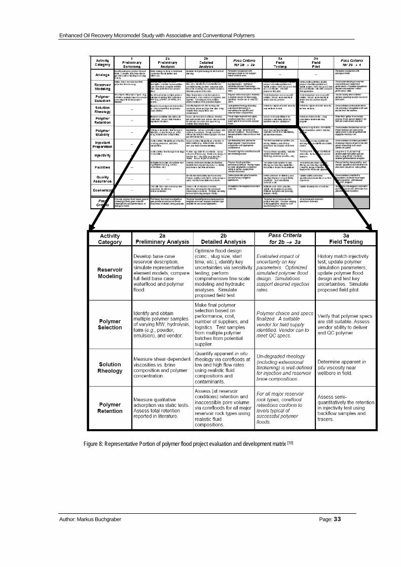
be passed in order to reach the next step of the workflow. The matrix in Figure 8 is a
useful document to manage those small activities. The most common subjects for
EOR projects can be found in the first column and are also listed below:
• Analogs
• Reservoir modelling
• Polymer Selection
• Solution Rheology
• Polymer Retention
• Polymer Stability

Enhanced Oil Recovery Micromodel Study with Associative and Conventional Polymers
Author: Markus Buchgraber Page: 30
• Injectant Preparation
• Injectivity
• Facilities
• Quality Assurance
• Economics
Analogs consist of specific case studies as well as general screening workflows based
on history of former polymer floods. General guidelines, which for example present the
key challenges for low permeable sands or high in situ temperatures, may be used.
Specific case studies should give positive and negative views of comparable projects.
Reservoir simulation is the key methodology to estimate the economic success and to
compare the polymer flood with alternative EOR techniques. Laboratory, geological
and field data are required to scale the physical phenomena and identify uncertainties.
Polymer selection starts at a very early stage of the planning. Different types of
polymers should be evaluated in terms of the molecular weight and degree of
hydrolysis when dealing with HPAM. Reservoirs with very high salinity may require
Xanthan polymer because of its better resistance against water hardness.
Polymer solution rheology depends on the polymer type, concentration, brine
composition and reservoir temperature. Since all of them are Non-Newtonian fluids,
they have different behaviour according to different shear rates. An important
parameter is the flow velocity near the wellbore and in the reservoir to get an estimate
of the later behaviour of the polymer solution.
Polymer retention has a major influence on flooding efficiency. It can reduce the
solution concentration and retard the transport through the reservoir by adsorbing the
polymer molecules on the rock surface and by trapping particles in small pores. Lower
permeable reservoirs are more likely to have polymer retention due to increasing rock
surface per unit mass and reducing pore throat size.
Polymer stability is usually connected to high temperatures. As a rule of thumb, 60°C
should be the limit but depending on the polymer and other reservoir conditions, there
are always exceptions. Thermal degradation is accelerated by adding oxygen or iron

Enhanced Oil Recovery Micromodel Study with Associative and Conventional Polymers
Author: Markus Buchgraber Page: 31
into the brine. As it can take up to one year to test those behaviours, such experiments
should be initiated at a very early stage.
Injectant preparation stands with the mixing of the right polymer solution. An over-
mixing shears polymers too much and results in degradation whereas an insufficient
mixing often includes non dissolved gel particles.
Injectivity depends on the injectant quality as well as on the polymer chemistry. Some
polymers can show a shear thickening behaviour at high velocities near the wellbore
and therefore reduce injectivity significantly. Another negative effect is that even a well
prepared polymer solution with high molecular weight can be trapped by narrow pore
throats and decrease injectivity slowly. Pilots to prove the required injectivity to be
technically and economically successful, are of major importance.
Facilities to generate and deliver the polymer solution have to be tested and certified
during the pilot project. To be on the safe side, any fitting valves and pumps which
produce high shear rates should be avoided in order to protect the polymer solution
from mechanical degradation.
Quality assurance of a polymer flood faces the following threats. Impurities in the
polymer powder caused during the transport, presence of oil or small amounts of
oxygen in the mixing water from the reservoir, poorly mixing or over-shearing the
polymers can degrade the polymer performance seriously. Defining quality checks at
different points and corrective actions in case of failure prevent any misleadings.
Economic assessments have to be done after each planning and performance stage
to make sure that the project is still worth being financed. Reservoir simulations,
laboratory and field studies should give a risk analyses in the early as well as in the
later stage of the project. The closer the end of the planning comes, the more accurate
and detailed should be the risk scenarios and possible uncertainties worked out and
identified [10].

Enhanced Oil Recovery Micromodel Study with Associative and Conventional Polymers
Author: Markus Buchgraber Page: 32
Figure 7: Staged process for polymer flood project evaluation and development [10]
Enhanced Oil Recovery Micromodel Study with Associative and Conventional Polymers
Author: Markus Buchgraber Page: 33
Figure 8: Representative Portion of polymer flood project evaluation and development matrix [10]

Enhanced Oil Recovery Micromodel Study with Associative and Conventional Polymers
Author: Markus Buchgraber Page: 34
Chemistry of EOR Polymers
EOR techniques basically use two types of water soluble polymers, which can be
divided into: polysaccharides produced from natural sources like wood, seeds or
bacteria and fungi, and polymers which are synthetically produced. At the moment the
most commonly used polymers are hydrolysed polyacrylamides (HPAM), which
belong the latter ones.
Polysaccharide Carbohydrates are generally described with Cm(H20)n. Saccharides are carbohydrates
with the formula CnH2n0n and can be divided into three groups: a) Monosaccharides,
b) Oligosaccharides, c) Polysaccharides. Polysaccharides are present as cellulose
building materials for cell walls, starch etc., it is a most abundant organic matter. The
chemical structure of hydroxyethyl cellulose is given below in Fig. 9, to have a better
chemical understanding. The basic unit is the cellulose. Within the ring there are three
positions which can be connected to different functional groups without destroying the
character of the ring. Those three positions are the CH2OH and the two hydroxyl
groups[11].
Figure 9: Molecular structure of hydroxyethyl cellulose [8]
For the hydroxyethyl cellulose, three CH2CHOH (hydroxyethyl) groups were added to
the possible positions. Other polymers can be obtained by adding different functional
groups like ethyl or carboxyl which would result in carboxylmethyl cellulose or
ethylhydroxylethyl cellulose.

Enhanced Oil Recovery Micromodel Study with Associative and Conventional Polymers
Author: Markus Buchgraber Page: 35
Xanthan
Xanthan, a polysaccharide, is produced by a bacterium called xanthomas campestris.
In order to protect the bacteria themselves from dehydration they produce the
polymer.
“The backbone of the molecule is a cellulose chain having two different sides at every
second glucose ring (ß-L glucose) like seen in Fig. 10. The side chains also have
saccharide rings as basic elements. Every side chain is made up of three
monosaccharides. The end of the first side chain begins with a mannose, followed by
gluceron acid, and then by a mannose having an acethyl group at the sixth carbon
atom. The second side chain is similar to the first one, but it contains a pyruvate unit at
the rear mannose. The distribution of the pyruvate within the molecule is not exactly
known. The pyruvate group and the two gluceron acids lend the molecule an anionic
character. Though like polyacrylamide this molecule also carries electrical charges at
its side chain, its behaviour is totally different in high salinity waters. The xanthan
molecule shows practically no decrease of viscosity yield as a function of rising
salinity. The reason for this is that the molecule, because of the side chain structure,
essentially stiffer than the polyacrylamide molecules. This may also be the reason for
its good shear stability. But if the pyruvate content becomes too high, the molecule
may behave similar to polyacrylamide with respect to its chemical stability
(precipitation, gel formation), and the adsorption may increase.” [8]
Other important polysaccharides for EOR are alginate, which reduces the water cut in
production wells and scleroglucan, which is produced by fungis and was tested for
polymer flooding as well. As the miceller may not be correctly removed from the high
viscous broth and thus plugging the formation in the wellbore, it has not been tested in
any further field applications.

Enhanced Oil Recovery Micromodel Study with Associative and Conventional Polymers
Author: Markus Buchgraber Page: 36
Figure 10: Molecular structure of xanthan[8]
Synthetic Polymers
Polyacrylamide
Polyacrylamides are water soluble polymers which are produced for many different
purposes. Deriving the acryl acid leads to the monomer acrylamide, which can be
seen in Figure 11.
Figure 11: Structure of polyacrylamide (not hydrolized) [8]
The range of the molecular weight is between 1*106-8*106 with an average particle
size between 0.1-0.3 μm.
During the hydrolysis in a water solution some of the CONH2 groups react and form
carboxyl groups (COOH), which dissociate in an aqueous solution. The properties of

Enhanced Oil Recovery Micromodel Study with Associative and Conventional Polymers
Author: Markus Buchgraber Page: 37
polyacrylamide in water solution are defined by the degree of hydrolysis and are taken
as an important parameter for the enhanced oil recovery. The structure of partially
hydrolysed polyacrylamide is shown in Figure 12.
Figure 12: Molecular structure of partially hydrolysed polyacrylamid[8]
The structure above represents a 25 percent hydrolysed polyacrylamide; in a pure
distilled water solution. The negative charges of the dissociated carboxyl groups react
so that the molecule chain is kept in a more or less stretched form, as the repulsion of
the charges have the same polarity. A very high viscosity is gained by the molecule
coil which occupies the largest possible volume. Small amounts of cations in the water
compensate the negative charges of the oxygen and the molecule coil tends to curl
and thus occupy smaller volumes in the aqueous solution. Another interesting
mechanism is the cross-linking of the molecules caused by higher amounts of divalent
cations. A too high concentration forms a gel like liquid or molecular aggregates,
which fall out of solution, are built.
Thus, polyacrylamide is a co-polymer consisting of acrylic acid and acrylamide. The
degree of hydrolysis is determined by the amount of acrylic acid in the molecule chain.
The usual amount of hydrolysis for enhance oil recovery polymer products is between
25-30%, but there are also products available with a zero degree of hydrolysis. Those
products are not as sensitive to salinity as comparable polymers with a higher
percentage of hydrolysis. For the purpose of polymer flooding, the latter has to be
used with higher concentration and hydrolysis can take place any time during flowing
through the reservoirs, which also has to be considered.
Additionally, the shear behaviour of HPAM plays an important role in the reservoir.
While shear thinning can be noticed at low to intermediate flow velocities, after
exceeding a critical flow velocity it becomes high shear-thickening. This high apparent
viscosity is produced when the polymer solution is flowing through a number of pore
bodies and throats in the reservoir and flow field elongation and contraction occurs.
When exceeding the critical velocity the polymer molecules do not have sufficient time

Enhanced Oil Recovery Micromodel Study with Associative and Conventional Polymers
Author: Markus Buchgraber Page: 38
to stretch and recoil and this elastic strain causes the high apparent viscosity. Higher
molecular weight HPAMs have a more shear-thickening behaviour than low molecular
weight HPAMs. [11] [12]
Associative Polymer
Associating water-soluble polymer is a relatively new class polymer, which was
recently introduced to oil field applications. Essentially, these polymers consist of a
hydrophilic long-chain backbone, with a small number of hydrophobic groups localized
either randomly along the chain or at the chain ends. When these polymers are
dissolved in water, hydrophobic groups aggregate to minimize their water exposure. In
aqueous solutions at basic pH, hydrophobic groups form intramolecular and
intermolecular associations, which rise to a three-dimensional network. This behaviour
increases the viscosity of polymer solution significantly. Another important fact is that
the functional groups on this polymer build more and stronger links with increasing
salinity which lead to higher viscosities compared to a conventional polymer solution
like polyacrylamides which decrease viscosity with increasing salinity. Former
experiments showed that they can also have shear thinning behaviour at high flow
velocities and shear thickening behaviour at intermediate flow velocities. To have both
lower pressure drops at the injection wells in order to achieve enough injectivity with
high velocities and higher viscosities in the reservoirs would be a highly preferable on
field applications [13]

Enhanced Oil Recovery Micromodel Study with Associative and Conventional Polymers
Author: Markus Buchgraber Page: 39
Polymer Degradation Mechanism
Three different types of polymer degradation have been known so far:
• mechanical degradation
• chemical degradation
• biological degradation
Biological Degradation
Biological degradation is mainly caused by bacteria or by chemical processes
governed by enzymes which destroy the polymer molecules. Enzymes catalyse
different processes in nature, like the hydrolysis of polysaccharide. These enzymes
are also called hydrolases. Such enzymes are used to remove gel plugs after a
polymer treatment. In most cases only biopolmyers undergo biological degradation at
lower temperatures and salinities.
Xanthan for example is destroyed by fermenting bacteria attacking the glucose units of
the molecular backbone under anaerobic conditions. To be on the safe side polymer
solutions should be tested under field conditions.
Mechanical Degradation
Mechanical degradation occurs when the polymer solution is exposed to high or very
high shear rates. Such conditions arise, during the mixing of polymer solution, flow
through chokes, injection through perforations or near well bore area where flow
velocity is very high. Polyacrylamide is the most sensitive one to mechanical
degradation, but nevertheless it is the most common used polymer for EOR.
Chemical Degradation
The main factor causing chemical degradation in an aqueous polymer solution is the
presence of divalent ions, oxygen and temperature. Cations such as Ca2+ ,Mg 2+,
influence its ability to flocculate and the solution stability by disturbing the hydrolysis of
polyacrylamides. Besides calcium and magnesium, Fe2+ is also present in small
amounts in the reservoir water. In combination with oxygen, which may be added

Enhanced Oil Recovery Micromodel Study with Associative and Conventional Polymers
Author: Markus Buchgraber Page: 40
during the mixing and handling process on the surface, iron cations may oxidize to
Fe3+ which in turn may flocculate polyacrylamides as well as polysaccharides.
Increased temperature may accelerate this process. As a rule of thumb
polyacrylamide can be used up to 70°C and a calcium concentration of 200 ppm.
Corresponding to water hardness this is a degree of 25, where 1 degree of hardness
is equal to 10 mg/l of CaO. In Fig. 13 the effect of water hardness on viscosity can be
seen.
Figure 13: Flow curves of a 1000 ppm polyacrylamide solution at different hardness of mixing water: 1.) 1.6°dH; 2.) 5°dH; 3.) 15°dH; 4.) 25°dH. (1°dH =10 mg CaO/l) [8]
To observe the sensitivity of the associative polymers to salinity, 3 different mixtures of
Superpusher 255 with 2000 ppm with increasing salinities were prepared and their
viscosity measured. Only light changes in their viscosity were observed as can be
seen in Fig. 14 [8]

Enhanced Oil Recovery Micromodel Study with Associative and Conventional Polymers
Author: Markus Buchgraber Page: 41
Figure 14: Influence of salinity on viscosity

Enhanced Oil Recovery Micromodel Study with Associative and Conventional Polymers
Author: Markus Buchgraber Page: 42
Rheological Behaviour of Polymers
Viscosity The basic measurement for any fluids such as liquids, semisolids or gases is their
viscosity. To understand the behaviour of the fluids and to force them according to the
needs in the reservoirs, it is essential to know their rheological relationship.
The definition of viscosity according to the Webster dictionary is the property of
resistance to flow in a fluid or semifluid[14]. Furthermore viscosity is defined as:
the ratio of the tangential frictional force per unit area to the velocity gradient
perpendicular to the direction of flow of a liquid [14].
The internal friction of a fluid is called viscosity. Friction occurs when a fluid layer is
moved in relation to another layer. The greater the force to initiate this movement,
which is called shear, the greater is the friction. Any movement of a fluid e.g.: spraying,
pouring, flowing is connected to a shearing. Therefore, high viscous fluids require
more force or shear to move than less viscous fluids. The figure below, Fig. 15, shows
the schematic definition according to Isaac Newton, where two parallel planes of fluid
with the same size and the distance dx are moving in the same direction with a
different velocities, v1 and v2.
Figure 15: Schematic picture of two planes moving in the same direction for shear rate calculation
The force to maintain the difference in speed was proportional to the velocity gradient.
The change in speed at which the intermediate layers move in respect to each other is
the velocity gradient. It is a measurement of shearing on the liquid and is called shear
rate. Below it is be symbolized as S and its unit is the reciprocal second (sec-1). The
second force is the shear stress, F´, which is defined by Eq.3 and has the unit of
dynes per square centimetre (dynes/cm²)

Enhanced Oil Recovery Micromodel Study with Associative and Conventional Polymers
Author: Markus Buchgraber Page: 43
After defining these two forces, viscosity, μ, can by defined as the ratio between shear
stress and shear rate see Eq. 4
The fundamental unit of viscosity measurement is the poise. A material requiring a
shear stress of one dyne per square centimetre to produce a shear rate of one
reciprocal second has a viscosity of one poise, or 100 centipoises. Newton assumed
that all materials have, at a given temperature, a viscosity that is independent of the
shear rate. In other words, twice the force would move the fluid twice as fast.
According to the rheological behaviour the fluids can be divided into two major groups
of fluids: a) Newtonian fluids, b) Non-Newtonian fluids
Newtonian Fluids
The characteristic graphical representation below in Fig. 16 shows the linear
relationship between shear stress and shear rate of a Newtonian fluid. The second
graph shows that there is no change in viscosity by changing the shear rate. The
majority of the fluids belong to the more complex Non-Newtonian fluids, but typically
Newtonian fluids are water or thin motor oil.
Figure 16: Characteristic rheological behaviour of Newtonian fluids[15]
Non-Newtonian Fluids
A common definition of Non-Newtonian fluids is that the relationship between F´/S is
not a constant. By changing the shear rate the shear stress will not vary in the same
portion or even in the same direction. Therefore, viscosity will also change with
increasing or decreasing shear rate. Viscosity measured that way is also called
apparent viscosity.

Enhanced Oil Recovery Micromodel Study with Associative and Conventional Polymers
Author: Markus Buchgraber Page: 44
Among the Non-Newtonian fluids there are several other groups of fluids which are
characterized by the way of changing their viscosity but for the purpose of this work
only the pseudoplastic and dilatants fluids are mentioned.
Pseudoplastic Fluids
This type of fluid will display a decreasing viscosity with an increasing shear rate, as
shown in Figure 17. Probably the most common of the non-Newtonian pseudo-
plastics fluids include paints, emulsions, and dispersions of many types. This type of
flow behaviour is sometimes called shear-thinning.
Figure 17: Shear rate determines viscosity in pseudoplastic fluids [15]
Dilatant
Increasing viscosity with an increase in shear rate characterizes the dilatant fluid; see
Figure 18. Although rarer than pseudo plasticity, dilatancy is frequently observed in
fluids containing high levels of deflocculated solids, such as clay slurries, candy
compounds, corn starch in water, and sand/water mixtures. Dilatancy is also referred
to as shear-thickening flow behaviour [15].
Figure 18: Shear thicking viscosity graphs [15]
The previous chapters were presented to get a better overview of polymer flooding
and to understand the physical properties of polymer solutions. The following part will
deal with the experimental apparatus and procedure in more detail.

Enhanced Oil Recovery Micromodel Study with Associative and Conventional Polymers
Author: Markus Buchgraber Page: 45
Experimental Apparatus
This chapter will list up all equipment used for the experiment and for gathering the
supporting data. The equipment consists of two parts: the injection system and the
data gathering system.
Injection System Two main parts build up the injection system:
1. Syringe pump (only for pumping water)
2. Vessels for gas (CO2), water, brine, polymer, oil
Syringe Pump
The syringe pump is a Teledyne Isco Model 100 DM (Fig. 19). The capacity of the
pump is 103 mL. The pump was only used to pump water. To avoid any damage of
the pump by pumping other fluids like brine or oil the vessel system is used.
The limit set up for the experiments are the following:
• The minimum flow rate: 0.0001 mL/min
• The maximum flow rate: 25.0 mL/min
• The minimum pressure: 10 psi
• The maximum pressure: 60 psi
Vessel
Vessels were equipped with a gauge at the top or bottom to control the fluid flow. To
fill up a vessel, it was connected with one end to the vacuum pump and with the other
end to the fluid which was sucked in. In Fig. 20 the vessel system for a brine injection
can be seen. Vessels were fixed to a holder in the vertical direction before the start of
an experiment.

Enhanced Oil Recovery Micromodel Study with Associative and Conventional Polymers
Author: Markus Buchgraber Page: 46
To connect vessels with the pump and to the micromodel, a 1/16” plastic tubing was
used. The advantage of plastic tubings is that with a visual control, bubbles in the
flowing system can be noticed early enough and in case of an eventual failure action
can be taken.
Figure 19: Teledyne Isco Model 100 DM syringe pump
Figure 20: Vessel system with decane and brine for water
Data Gathering Equipment
Microscope
A Nikon Eclipse ME 600 (Fig. 22) with a metal halide lamp is used for this study. An
adapter mounted on the microscope allows the surveillance of the pore spaces via a
camera. Both videos and pictures are taken through this adapter. Three different
magnifications were used to observe the micromodel: 40X, 100X and 200X. Optical
properties of these lenses can be seen in Tab. 1.
Magnification Working
Distance (mm) Aperture
Viewable
Diameter(µm)
4X 17.1 13 5500
10X 16.0 0.3 2200
40X 7.4 0.45 1100
Table 1: Optical properties of microscope lenses [16]

Enhanced Oil Recovery Micromodel Study with Associative and Conventional Polymers
Author: Markus Buchgraber Page: 47
Camera
A Nikon Coolpix P5100 is used to collect pictures at micro and meso scale. High
magnification micro images are taken with support of the microscope, whereas meso
scale photographs are taken with a diffusion box.
Viscometer:
A digital Brookfield DV-II-Pro+© viscometer, Fig 21, was used for the viscosity
measurements of oil and polymer solution. Calibration of the viscometer was done by
using Brookfield calibration fluids of 10 cp and 100cp. The measurements were done
with a spindle adapter. The viscometer allows a measurement range from 0.1cp to
10000 cP. Additionally a water bath can be used to measure fluids at a specific
temperature.
Figure 21: Brookfield viscometer with example beaker and spindle for measurements
Figure 22: Nikkon Eclipse microscope

Enhanced Oil Recovery Micromodel Study with Associative and Conventional Polymers
Author: Markus Buchgraber Page: 48
Micromodel
Early micromodel experiments simply used capillary tubes with different diameters and
lengths to study the miscibility or displacing process of different fluids or phases.
Those models where followed by Hell Shaw models which consist of two glass plates
with a narrow space in between to allow fluid flow. Later on this space was filled with
glass beads in order to build a kind of artificial porosity and permeability. They were
simple models and could not count for real rock and pore geometries or properties.
“Micromodels can be used to study the flow behaviour on a pore scale. They are
patterns of a porous medium etched on a silicon or glass surface and hence are
representative of the two dimensional structure of the porous medium. Micromodels
have been extensively used to study the flow behaviour in multiphase flow, oil-foam
interaction studies, solution gas drive, contaminant hydrogeology, etc. The patterns
used in the construction of the porous medium may be prepared from thin sections of
the porous medium to actually represent the medium or in several cases are
geometrically constructed as series of repeatable simple or complex geometric figure
aggregates. However as the micromodels represent a two dimensional porous
medium, flow problem, extrapolation of results to the three dimensional flow problem
occurring in the real porous medium needs to be done with certain amount of caution.
It has also been observed that a non uniform etch depth in the micromodels may lead
to snap-off situations not consistently predictable with the flow behaviour (Rossen,
1999). Another constraint of the micromodels regarding dimensionality is the lower
macroscopic connectivity and co-ordination number (Nguyen, et al., 2000). Though
both etched glass and silicon micromodels have been used, glass micromodels
because of the nature of their fabrications have pores whose sizes are several times
larger than the actual size.” [17]
A brief summary of the use of micromodels for various applications is listed below.
The first etched-glass micromodel was developed by Mattex and Kyte. Straight
interconnected flow channels built up the network. It was a very good approach to
observe and visualize flow behaviour. [18]
A further development of the micromodel was achieved by Davis and Jones[19]. They
worked on the drawbacks and limitations of the micromodel and came up with a new
fabrication technique. A photosensitive fluid, which was resistant to several solvents
after beeing exposing to ultraviolet light, was coated on glass. Hence, they were able
Enhanced Oil Recovery Micromodel Study with Associative and Conventional Polymers
Author: Markus Buchgraber Page: 49
to produce more complex pore structures, which met the requirements for more
realistic experiments.
In 1987 Owete and Brigham [20] used silicon-wafer micromodels for further
development. Their special material characteristics allowed a better control of the
etching process and therefore also the etching depth. With this new technique a more
detailed and complex artificial pore network was etched in the micromodel. Because
the silicon wafer is initially not water wet, they also worked on a technique to coat the
surface of the silicon wafer with a thin dioxide film to create water wet conditions. The
etched flow channels in the micromodel were sealed with a pyrex glass by an anodic
bonding process to allow visual observation. Drilled inlet and outlet ports at the
corners of the micromodel allowed the fluid communication.
Hornbrook [21] produced the first micromodels, which were almost identical to original
Berea sandstone. Geometrical and topological properties as well as wettability and
pore roughness were close to an original core sample. Micromodel pore structure was
based on a thin section of a Berea sandstone. With a scanning electron microscope a
high resolution photograph was taken and digitally processed. The drawback of this
technique is that the SEM captures only a very little portion of the thin section. Hence
the edges of the photograph had to be processed to loop this unit cell image together
and to provide connectivity between the edges to fill a 5cm x 5 cm area.
In 1996 Keller [22] used the micromodel to observe the flow behaviour of three phases.
The pressure limitations allowed not more than 35 psi. Exceeding this limit led to a
material failure and to an abortion of the experiment. For higher pressures special
experimental equipment had to be used.
Campbell and Orr [24] performed the first high pressure experiments for the
displacement of oil by CO2. To handle these elevated pressures the micromodel was
housed in a pressure vessel[23] .
A more detailed description of high pressure micromodel applications can be found in
the work of Gorge (1999). [17]
In this study the micromodel structure and design is almost identical to Berea
sandstone in terms of pore geometry and topology.

Enhanced Oil Recovery Micromodel Study with Associative and Conventional Polymers
Author: Markus Buchgraber Page: 50
Micromodel Fabrication
A simple micromodel holder for low pressure systems was used, fabricated from
aluminium for the experiments in this case. Basically the micromodel represents a two
dimensional network of a porous medium on a silicon wafer. First attempts used
etched glass wafers to provide the artificial pore structure, but because of the
limitations and disadvantages reported above, glass wafers were replaced by silicon
wafers involving the visualization of the flow behaviour on pore scale.
A scanning electron microscope (SEM) image of a reservoir rock thin section acts as
the basis of a typical micromodel, see Fig 23. However such a pattern needs some
digital modification at the edges to ensure continuity in the porous medium. The
pattern etched on the micromodels for these experiments was taken from a random
hand drawn pattern, which represents the two dimensional structure of the porous
medium. The grains of this pattern are range from 50 to 100 μm. Small and large
pores, channels and very narrow throats build up the artificial network in the unit cell
and made it similar to a real reservoir rock.
Figure 24 represents the unit cell which was repeated several times to fill up an area
with the dimensions of 5cm x 5cm. In Fig. 25 the looped unit cell is presented.
Figure 23: SEM image of a thin section of a Berea Sandstone [25]

Enhanced Oil Recovery Micromodel Study with Associative and Conventional Polymers
Author: Markus Buchgraber Page: 51
Figure 24: Unit cell of the micromodel [17]
Figure 25: Repeating units of the micromodel[17]
To guarantee that the pattern is continuous, the edges had to be arranged, to sit
together like a jigsaw puzzle. But the key features of the micromodel are the inlet and
outlet channels or fractures and ports. They enable the displacement process to work
in a linear way along the edges and not like a radial displacement which can be
observed in a five spot pattern. A schema of the model with the features described
above can be seen in Fig. 26

Enhanced Oil Recovery Micromodel Study with Associative and Conventional Polymers
Author: Markus Buchgraber Page: 52
Figure 26: Schematic picture of the micromodel with inlet and outlet fracture and ports [17]
The construction of the micromodel incorporates several stages until it can be used for
an experiment. The micromodels were produced at the Stanford Nanofabrication
Facility (SNF). The SNF is a clean room facility for Micro Electronics Research
Scientific, where structures up to a range and resolution of 5 Angstrom can be etched.
Each of these models had to run the same procedure and should be a replica of the
basic lithography mask image model. Micromodels cannot be bought, they have to be
produced manually. As the production of these high-tech models was a major part in
the experiments and works, it is mentioned in more detail in the following chapter.
As reported above, a 2D etched network forms the basis of the micromodel and
represents the porous medium. To seal those silicon channels, another plate with the
same size and with transparent characteristics is added on the top. The transparency
of this top plate enables the visual observation through a microscope or an attached
camera and gives the required high resolution micro scale pictures of the pore scale
displacement.
Once the thin section of a Berea sandstone is taken and the structure put on a chrome
mask, also called lithography mask, the manufacturing process for micromodels can
start as listed below:
Inlet port of inlet fracture
Inlet port of outlet fracture Outlet port of outlet fracture
Outlet port of inlet fracture
Outlet fracture
Inlet fracture

Enhanced Oil Recovery Micromodel Study with Associative and Conventional Polymers
Author: Markus Buchgraber Page: 53
Imaging : A photosensitive chemical is sprayed on the silicon wafer, which is then
exposed to ultraviolet light through the mask on top. After exposing the photoresist is
selectively removed during the developing step.
Etching: The developed wafer is then etched with hydrofluoric acid to produce a
micromodel with an etch depth of around 25-30 μm on the silicon wafer.
Cleaning and Bonding: The silicon wafer with the etched pattern is first cleaned in a
sulphuric acid cleaning and then bonded to a glass plate to create a flow medium.
The schematic of the steps described above can be seen in Fig. 27
Figure 27: Micromodel fabrication: a) Coating with photoresist; b) Exposing and developing; c) Etching; d) Bonding
The next chapter will describe the above steps in more detail and show where
precautions have to be taken in order to produce a perfect micromodel.

Enhanced Oil Recovery Micromodel Study with Associative and Conventional Polymers
Author: Markus Buchgraber Page: 54
Micromodel Pattern Preparation
The structure of the repeated unit cell is a handmade drawn pattern and incorporates
the entire feature of a real reservoir rock with comparable dimensions. The software,
L-EDIT is required to do the preparation of the pattern, which is available at the SNF
lab. A file which is compatible and needed for the mask-making machine is produced.
The major tasks, which have to be done when preparing the mask with the software
are:
• Design of the repeatable unit cell having the features of the porous medium
• Design of the inlet and outlet ports and channels of the entire micromodel
assembly.
To enable the communication with fluids through the micromodel, inlet and outlet ports
are required. These ports can be seen in Fig. 26 and are in the middle of the squared
boxes at the four corners of the micromodel. For polymer or water floods, all four ports
are necessary to clean the inlet fracture in order to achieve a linear displacement.
When the software work is done, the pattern can be reproduced on a glass chrome
plate, which is called mask. The mask making is not done in SNF since it is very
complicated. Only one mask is required and can be used to produce thousands of
micromodels. Fig. 28 shows the mask used to produce the pore pattern for these
experiments.
Figure 28: Lithography mask, coated with chrome

Enhanced Oil Recovery Micromodel Study with Associative and Conventional Polymers
Author: Markus Buchgraber Page: 55
Wafer Imaging
There are a lot of manufactures selling silicon wafers which differ in surface roughness
size, resistivity and price. For manufacturing the micromodels a doubled polished
silicon wafer of the type K-Test is used. Starting the processing of the micromodel, the
wafer is coated with a 2 μm thick layer of Shipley 3612 photoresist (Fig. 27 a), without
edgebead removal (edgebead removal is the process in which a small ring of
photoresist is removed around the wafer).
It is of crucial importance that the wafers are not wet and do not contain any moisture
on the surface before being coated with the photoresist. New wafers which are sealed
in a box, can be directly processed and coated. If the sealing of a box is already
broken and the wafers are old or have been exposed to air, they need to be baked in a
singe oven at a temperature of 150°C for 20 minutes before being coated with
photoresist. When using the sing oven a special cartridge is required, this has a very
high thermal resistance and is made of Teflon to prevent melting.
Once the coating process is over the wafers should be exposed to ultra violet light
within 2 to 3 hours to guarantee the best possible result. The coating, exposing and
developing steps are all done in a special yellow light area in the SNF lab. Any other
light would destroy the characteristics of the photoresist. So at no time during these
processes the wafer has to be taken out of this area. The mask used in the process of
exposing the wafer to the ultraviolet light needs to be cleaned every time before use,
to prevent exposing dirt marks and dust particles. The cleaning is done at a wet bench
in the following strict order: acetone, methanol and isopropanol.
A final wash with de-ionized water and N2 jet makes the lithography mask ready to be
used. While exposing the resist coated wafer to ultraviolet light, it is important to make
sure that the mask and the wafer are aligned, to prevent the pattern from being off
centre on the wafer. During this process parts of the wafers which represent the pore
channels of the micromodel at the end, are hit by the ultraviolet light. At this part the
photoresist is getting unstable. Areas which are protected by the chrome of the mask
do not have any contact to ultraviolet light and stay stable. An exposure of 3 to 4
seconds to the ultraviolet light is sufficient to make the photoresist unstable. During the

Enhanced Oil Recovery Micromodel Study with Associative and Conventional Polymers
Author: Markus Buchgraber Page: 56
developing step, which is a chemical wash, the unstable parts of the photoresist are
selectively removed (Fig. 27 b)
Wafer Etching and Finishing
The developed wafers are taken out of the yellow light area and can be further
processed in the SNF lab. The etching process utilizes hydrofluoric acid gases to etch
a depth of approximately 25 μm ± 3 μm.
In the figure below (Fig. 29) a SEM image of a the etched pattern can be seen.
Figure 29: SEM image of etched micromodel. Pore diameters between 10 μm -150 μm [25]
After the etching the wafers have to be cleaned in a sulphuric acid/ hydrogen peroxide
piranha solution (9:1 H2SO4:H2O2) to remove any residual photoresist or precipitation
product from the etching process.
The drilling of the four holes which later allows the communication of the fluids with
the micromodel is made at a different lab. After drilling the wafers are taken back to
the SNF where a 15 min intensive cleaning procedure with a sulphuric acid/ hydrogen
peroxide, piranha solution, (9:1 H2SO4:H2O2) removes any residual moister. The last

Enhanced Oil Recovery Micromodel Study with Associative and Conventional Polymers
Author: Markus Buchgraber Page: 57
step is done outside the SNF where the wafer is heated on a hot plate at 700°F for 30
minutes.
This is done to oxidize the silicon to form a thin film of silicon dioxide on the surface.
As a consequence the surface gets water wet. As a final step the wafer is bonded with
an anodic bonding to a glass plate to complete the flow system. During the bonding a
wire gauze with a weight is placed on the top of the silicon wafer and a potential of
1000 volts is applied for 1 hour. The elevated temperature causes the sodium ions on
the glass plate to move and to attract the negative electrode on the glass surface,
where they are neutralized to form a bond. Pyrex is used because of its similar thermal
expansion coefficient to silicon: pyrex: 3.25 x 10⁻⁶ / °C; silicon: 2.56 x 10⁻⁶ /°C. Figure
30 shows a bonded micromodel ready to use.
Figure 30: Bonded micromodel [16]
Micromodel Holder The micromodel is placed in a holder which has conduits connected to the plumbing of
the setup as shown in Fig. 33. This holder is fabricated from aluminium and consists of
two inlet and two outlet ports, which communicate with the micromodel at the drilled
holes. The ports are sealed with viton O-rings, Fig. 34. These rings need replacement
after a few runs. Figure 31 shows a schema of the micromodel holder

Enhanced Oil Recovery Micromodel Study with Associative and Conventional Polymers
Author: Markus Buchgraber Page: 58
Figure 31: Micromodel holder sketch
Figure 32: Micromodel with O-rings graving
Figure 33: Micromodel holder with fixed micromodel
Figure 34: O-ring graving without and with o-ring

Enhanced Oil Recovery Micromodel Study with Associative and Conventional Polymers
Author: Markus Buchgraber Page: 59
Experimental Procedure
The aim of the experimental procedure and preparation was to have exactly the same
or at least very similar initial conditions for every experiment. Therefore, each
experiment had the same workflow:
• Clean micromodel holder and micromodel
• Saturate micromodel with brine (calculate permeability)
• Saturate micromodel with oil (take pictures to determine Swi)
• Dismantle the micromodel holder and clean holder as well as micromodel.
Reassemble holder and micromodel
• Start the flood with polymer solution or brine and take meso scale pictures
during the flood and micro scale pictures after breakthrough and after 22 hours
This section of the thesis will report the specific work steps of the experiment
Clean Micromodel Holder and Micromodel
The cleaning of the micromodel holder is the first step of an experiment. When
pumping polymer solution through the micromodel, small polymer precipitations form
at the inlet ports of the holder. These small particles can get loose during the next
experiment when saturating with water or oil and cause a plugging of the pores, which
would result in changed initial conditions. By using a vacuum pump, toluene, isopropyl
alcohol (IPA) and water the four entry ports of the holder and the o-rings can be freed
from oil and polymer solution.
During the first water flood experiments, the micromodel could be cleaned and reused
for the next experiment. Because of the irreducible plugging of the pores, the
micromodels could not be cleaned when using a polymer solution. When cleaning
micromodels, the following procedure is used.
“Flush with isopropanol (IPA) to remove some residual oil and flush with IPA at
constant pressure (P=50psi). In this set-up water pushes IPA into the
micromodel/micromodel holder assembly. Once IPA begins to flow out of the outlet

Enhanced Oil Recovery Micromodel Study with Associative and Conventional Polymers
Author: Markus Buchgraber Page: 60
port of the inlet fracture, cap this port. Continue to pump IPA for 1mL, or until there is
only immobile oil in the micromodel.
Pump with toluene to remove the remaining residual oil: Pump toluene into the
micromodel at pressure <50psi; once toluene is noted at the outlet port of inlet
fracture, cap this port. Continue pumping at P<50psi until micromodel appears to be
clean. At this point, there should be no visible oil, or at the most a few immobile
patches of residual oil.
Pump with carbon dioxide to remove the toluene: Disassemble micromodel holder.
Use vacuum and heat lamp to remove and vaporize residual toluene in the holder. A
heat lamp is positioned about 8 inches above the micromodel/micromodel holder
assembly while CO2 floods the micromodel at constant pressure. Carbon dioxide is
pumped until toluene is removed. If streaky spots persist, check under microscope to
ensure that there is no visible toluene in the micromodel; the streaks are due to
toluene adhering to pore grain surface. If any residual oil remains in micromodel,
repeat steps three and four as necessary.
Pump with IPA: Repeat step 2, except that the end point is achieved 1 mL after the
micromodel is 100% saturated with IPA. Any streaks noted in step four should be
removed by the IPA. The micromodel is clean and is ready to be fully saturated with
water” [16]
Saturate Micromodel with Brine
After cleaning the micromodel or using a new one, it has to be saturated with brine.
After oil saturation small amounts of brine stay in the model and act as the initial water
saturation. In Fig. 35 the setup for this step is presented.
The water pump provides water through a 1/16 inch plastic tubing with a constant
pressure of 40 psi into the bottom of a decan vessel. The lighter decan is forced out at
the top of the vessel and flows into the top of the brine vessel. The heavier brine is
pushed towards the vessel and goes from the bottom of the brine vessel into the inlet
port of the micromodel inlet fracture. As soon as brine comes out of the outlet port of
the inlet fracture, the outlet port is closed. About 5-10 ml of brine has to be flushed

Enhanced Oil Recovery Micromodel Study with Associative and Conventional Polymers
Author: Markus Buchgraber Page: 61
before all CO2 bubbles are gone. To make sure that no CO2 is left in the micromodel, it
has to be checked with the microscope. When increasing the pump pressure from 40
psi to 55 psi or 60psi trapped CO2 is usually dissolved in the brine. Any CO2, which
cannot be removed during brine saturation will stay till the end of the experiment and
can falsify results. In Fig. 36, CO2 trapped in a brine saturated micromodel can be
seen.
Figure 35: Experimental setup for brine saturation
Figure 36: Brine saturated micromodel with trapped CO2 (white bubbles)
If the micromodel is 100% water saturated, the permeability can be measured like
reported below.
Brine
Micromodel
Water
pump
Decan

Enhanced Oil Recovery Micromodel Study with Associative and Conventional Polymers
Author: Markus Buchgraber Page: 62
Permeability Measurement
Permeability measurements before each experiment were part of the quality control
and should ensure that the initial conditions for all experiments are the same. Because
of discrepancies during the last experiments permeability measurements were
performed in two different ways to have a quality check.
1. The micromodel is flooded with water with 4 different flow rates and pressures and
their corresponding pressure drops and flow rates are measured. Permeability is
calculated according to Darcy´s Law.
2. The micromodel is flooded with CO2 at different pressures. With a bubble flow meter
which is connected to the outlet of the micromodel flow rates are measured (Fig. 37)
and the permeability can be calculated with Darcy´s Law.
The working principle of a bubble flowmeter is the following:
A soapy solution can be found at the bottom of the bubble flow meter. CO2 from the
micromodel frees single bubbles and forces them upwards the glass column.
The time that a bubble (CO2) needs to flow from point x1 to x2 (see Fig. 37) is
measured. The distance from x1 to x2 marks a defined volume of 1 cm³. With these
data the flow rate can be calculated which is used for Darcy´s calculations.
Figure 37: Schematic view of permeability measurement with a bubble flow meter
The three different results of a measurement are presented below: constant pressure
(Tab.2), constant flow rate (Tab. 3) and bubble flow meter (Tab.4). In practice all the

Enhanced Oil Recovery Micromodel Study with Associative and Conventional Polymers
Author: Markus Buchgraber Page: 63
measurements are averaged and a final average value out of three values is
calculated. In the example below this would result in 918 md.
INPUT OUTPUT
P2
(psig)
P2
(atm)
P1
(atm)
Q
(mL/min)
Q
(mL/s)
Area
(cm^2)
L
(cm)
viscosity
(cP) k (darcy)
40 3.72 1.00 0.378 0.0063 0.0125 5 1.0 0.92
30 3.04 1.00 0.277 0.0046 0.0125 5 1.0 0.90
20 2.36 1.00 0.179 0.0029 0.0125 5 1.0 0.87
10 1.68 1.00 0.088 0.0014 0.0125 5 1.0 0.86
average 0.89
Table 2: Permeability measurements with constant pressure
INPUT OUTPUT
P2
(psig)
P2
(atm)
P1
(atm) >
Q
(mL/min)
Q
(mL/s)
Area
(cm^2)
L
(cm)
viscosit
y (cP) k (darcy)
37 3.52 1.00 0.35 0.0058 0.0125 5 1.0 0.92
32 3.18 1.00 0.3 0.005 0.0125 5 1.0 0.91
21 2.43 1.00 0.2 0.0033 0.0125 5 1.0 0.93
11 1.75 1.00 0.1 0.0016 0.0125 5 1.0 0.89
average 0.91
Table 3: Permeability measurements with constant flow rate
40 psi 30 psi 20 psi 15 psi 10psi
time (sec) time (sec) time (sec) time (sec) time (sec)
1 0.81 1.25 2.4 3.65 6.13
2 0.85 1.3 2.38 3.64 6.06
3 0.87 1.27 2.44 3.66 6.22
4 0.88 1.31 2.47 3.66 6.15
5 0.84 1.24 2.44 3.62 6.1
940 md
Table 4: Permeability measurement with bubble flow meter

Enhanced Oil Recovery Micromodel Study with Associative and Conventional Polymers
Author: Markus Buchgraber Page: 64
Saturate Micromodel with Oil
After being saturated with water, the micromodel is ready to get oil saturated. For oil
saturation, the same apparatus as in Fig. 38 is used. Water from the pump flows into
the bottom of the oil vessel and pushes the oil towards the top of the vessel from
where it goes through the tubing into the inlet port of the inlet fracture. The whole
process is run with a constant pressure of 55 psi.
It is not required to cap the outlet port of the inlet fracture when oil is dropping out of
the port, since the oil acts as a plug in the very narrow outlet port. The oil saturation is
one of the critical parameters during an experiment. Final oil saturations can vary
between 90-98% although no changes in pore structure or etching depth is observed
or measured. Even extended oil saturation periods with abnormal high pump
pressures do not increase the oil saturation for the micromodels with 90% saturation.
Depending on the micromodel, connate water saturation was reached after 2 to 8
hours.
According to Fig. 41 saturation does not change a lot with time. Meso scale pictures
often indicate a uniform and fully saturated micromodel, but by having a closer look at
micro scale pictures, changes in oil saturation can be significant. Fig. 39 and Fig. 40
show two different pictures after eight hours of oil saturation.
Figure 38: Setup for oil saturation with water pump and oil vessel

Enhanced Oil Recovery Micromodel Study with Associative and Conventional Polymers
Author: Markus Buchgraber Page: 65
Figure 39: Well oil saturated micromodel (brown: oil; white: grains and water)
Figure 40: Poor oil saturated micromodel
Figure 41: Oil saturation in relation to time

Enhanced Oil Recovery Micromodel Study with Associative and Conventional Polymers
Author: Markus Buchgraber Page: 66
After checking the process on micro and meso scale, micro scale pictures are taken
and initial water saturation Swi can be calculated. In case of a not satisfying oil
saturation, even after a long time, the model has to be cleaned and the process
repeated. A typical sequence of meso scale pictures after periods of time can be seen
below in Fig. 42. Picture a.) demonstrates oil entering the micromodel matrix and filling
up the inlet fracture towards the end of the outlet port.
The saturation propagations follows a radial way as long as the fracture is not fully oil
saturated. After the oil has reached the outlet port, saturation continues in a more
linear way. In picture d.) the outlet fracture starts being saturated. The last photograph
f) represents a perfect uniform oil saturated micomodel which is ready for a polymer
flood. Fig. 43 represents a sequence of oil saturation at micro scale. In former
experiments, a heat lamp was used to lower viscosity of the oil and to reach saturation
faster. Because of several broken wafers, caused by thermal cracking during this
process, the heat lamp was avoided for this series of experiments.

Enhanced Oil Recovery Micromodel Study with Associative and Conventional Polymers
Author: Markus Buchgraber Page: 67
Figure 42: Meso scale oil saturation after time (from the left top to the right bottom: a,b,c,d,e,f)
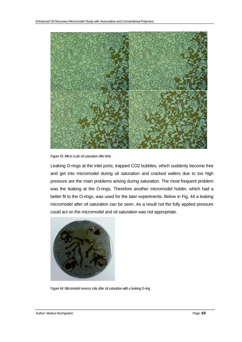
Enhanced Oil Recovery Micromodel Study with Associative and Conventional Polymers
Author: Markus Buchgraber Page: 68
Figure 43: Micro scale oil saturation after time
Leaking O-rings at the inlet ports, trapped CO2 bubbles, which suddenly become free
and get into micromodel during oil saturation and cracked wafers due to too high
pressure are the main problems arising during saturation. The most frequent problem
was the leaking at the O-rings. Therefore another micromodel holder, which had a
better fit to the O-rings, was used for the later experiments. Below in Fig. 44 a leaking
micromodel after oil saturation can be seen. As a result not the fully applied pressure
could act on the micromodel and oil saturation was not appropriate.
Figure 44: Micromodel reverse side after oil saturation with a leaking O-ring

Enhanced Oil Recovery Micromodel Study with Associative and Conventional Polymers
Author: Markus Buchgraber Page: 69
Cleaning After Oil Saturation
The most critical part of the experiment is the start of the flood, where the inlet fracture
has to be cleared in order to achieve linear displacement. In former times, the flooding
fluid was directly connected after completing the oil saturation. As a result the cleaning
of the inlet fracture of the oil took several hours and was insufficient for a perfect
displacement most of the time. In other words, the displacing fluid started to get into
the micromodel before the complete fracture was cleared and the outlet port at the
inlet fracture capped.
Different cases of cleared fractures when capping the outlet port of the inlet fracture
can be seen in Fig. 45. As a consequence the micromodel was taken apart after oil
saturation since February 2008. Micromodel, micromodel holder, entry ports and the
backside of the micromodel are cleaned with toluen and water and then re-assembled.
To avoid any air bubbles between entry ports and micromodel, the micromodel entry
ports are filled with water or polymer solution before re-assembling the holder. This
procedure enabl a very fast and improved cleaning of the inlet fracture and guarante a
better linear displacement.
Figure 45: Inlet fractures from different experiments with different stages of clearness. From top to bottom decreasing clearness.

Enhanced Oil Recovery Micromodel Study with Associative and Conventional Polymers
Author: Markus Buchgraber Page: 70
Starting the Flood
After the holder has been cleaned and re-assembled the displacing fluid (water, or
polymer solution) can be connected to the oil saturated micromodel. The setup can be
seen in Fig. 46. Water pushes the polymer solution towards the bottom of the vessel
and enters the micromodel.
At the beginning of the flood the polymer solution is injected at a constant pressure of
10 psi to clean the fracture from oil. Once the fracture is free and the polymer solution
is dropping out of the outlet of the inlet fracture the outlet port is capped. Then the
pump is switched from a constant pressure to a constant flow rate of 0.0001 ml/min.
The micromodel is put into the diffusion box for meso scale pictures to be taken. Once
the polymer solution reaches the outlet fracture the micromodel is placed under the
microscope where micro scale pictures are taken. Then, the flood is continued for 22
hours which represent 10 pore volumes. After that period, micro scale pictures are
taken to determine the ultimate recovery. A typical series of pictures at the front of a
polymer displacement can be seen in Fig. 47.
Figure 46: Polymer flooding set up with water pump and polymer vessel

Enhanced Oil Recovery Micromodel Study with Associative and Conventional Polymers
Author: Markus Buchgraber Page: 71
Figure 47: Micro scale pictures at the displacing front after different time intervals (5 sec: 10 sec; 15sec; 20 sec)

Enhanced Oil Recovery Micromodel Study with Associative and Conventional Polymers
Author: Markus Buchgraber Page: 72
Image Analysis
Results of recovery and swept area are necessary to evaluate the experimental
success. A major drawback of the micromodel is the missing possibility to perform any
material balance.
Inlet ports and O-ring cravings occupy 10 times greater volume than the micromodel
matrix. This huge dead volume is a serious problem in measuring the volume of the
displacing or displaced phases. Additionally, the amount of liquid used for a whole
experiment is so small that it does not reach the outlet port of the outlet fracture and
therefore it cannot even be collected for measurement. Several other attempts to
reach a material balance with weighting and using finer injection ports were not
successful.
So, as a consequence, 25 high resolution photographs of the pore structure in the
micromodel are taken to determine irreducible water saturation (Swi), water saturation
at breakthrough (Sbtp) and residual oil saturation (Sor). To make sure that the whole
area of the model is captured the micromodel is subdivided into 25 equally sized
rectangles, Fig 48. At specific times, one single photograph of each rectangle is taken.
These moments are first after oil saturation to determine Swi, secondly after
breakthrough of the polymer solution at the outlet fraction to determine the Sbtp, and
finally, after 22 hours which refers to 10 swept pore volumes of the micromodel to
determine Sor. The pictures are taken with a Nikon Coolpix P5100 and with a Nikon
Eclipse ME 600
.

Enhanced Oil Recovery Micromodel Study with Associative and Conventional Polymers
Author: Markus Buchgraber Page: 73
Figure 48: Micromodel grid for taking micro scale photographs
Figure 49 represents a photograph of a micromodel at Swi at a 10X magnification,
which is ready for a polymer flood at this point. These photographs are manipulated
and analysed digitally in MATLAB or G.I.M.P. to calculate the saturations mentioned
before. This post experimental procedure is imprecise due to the shadow of the pore
grain/space interface, and therefore yields relative saturation values.
Figure 49: Saturated micromodel ready for a polymer flood

Enhanced Oil Recovery Micromodel Study with Associative and Conventional Polymers
Author: Markus Buchgraber Page: 74
Image Analyse in G.I.M.P.
The very first experiments were post processed with the photostudio program G.I.M.P.
To obtain values for saturation, the colour histograms for each single picture had to be
analysed. In Fig. 50, the RGB histogram of the picture above is shown.
The three humps represent the three different colours, brown for the oil, black for the
grain edges and white for water, polymer solution and grains. The further processing
of the pictures required a manually determination of the threshold values. In other
words to define a limit, at which everything more colour intensive or brighter is white
and everything less intensive or darker is black. As shown in Fig. 51, the blue area
marks the parts which are white after processing.
As a result of this threshold procedure, a black and white picture is obtained. In this
picture the black and white pixels are counted automatically and give the saturation
values.

Enhanced Oil Recovery Micromodel Study with Associative and Conventional Polymers
Author: Markus Buchgraber Page: 75
Figure 50: Typical micromodel histogram of a micro scale picture. Three humps represent oil, polymer or water saturation, grain edges and grains from the left to the right
Figure 51: Histogram with threshold limit (blue area)
Figure 52: Histogram after setting a threshold value and converting into a binary picture. The bars at the beginning and the end of the diagram represent the frequency of black and white.

Enhanced Oil Recovery Micromodel Study with Associative and Conventional Polymers
Author: Markus Buchgraber Page: 76
Figure 53: Processed binary image of Figure 49
The problem of this procedure was that it was not possible to automize the procedure.
Therefore every single threshold value had to be defined manually which in fact is not
very precise either. So, another method was found to make the image analyses in a
more precise and faster way.
Image Analysis in MATLAB
The primary hindrance in accurately calculating the saturation values is that a
significant minority of the pore space is obscured by the shadow cast, by the pore
grains and the shadow at the oil-water interfaces. Figure 54 shows an unetched
micromodel, meaning that the wafer was only exposed and the photoresist was
selectively removed. Whereas Fig. 55 presents an etched ( to 25 μm) and bonded
model. When comparing the two pictures a lack of a gap between the grains is
obvious. In the etched wafer, the grains appear to be touching each other and seem to
be closer together. This shadow makes it impossible to determine which fluid occupies
this space when calculating saturations. As a consequence, only the space which can
be seen is considered as pore space for the image analyses. About 20-30 % of the
pore volume is lost because of these shadows.

Enhanced Oil Recovery Micromodel Study with Associative and Conventional Polymers
Author: Markus Buchgraber Page: 77
Figure 54: Only coated and exposed micromodel (not etched)
Figure 55: Etched empty micromodel
A 100% water saturated micromodel can be seen in Fig.56 and Fig. 57 before and
after being processed with image software. The black lines cover about 25% of the
total picture and contribute to 26% of the pore space. When having a closer look at
Fig. 58, it can be seen that the lines are getting thicker towards the edges of the
photograph. The developed MATLAB routine (Appendix A) automatically crops and
removes the portion of the image which is unevenly illuminated. This distorting effect is
caused by the adapter which is not 100 % centred adapter. The RGB (red, green,
blue) colour ranges for oil in the photographs are determined by manually sampling
the values for oil in a few of the 25 pore scale photographs. During the further
processing, MATLAB converts the colour images to binary images, which black
represents oil and grain shadows and white indicates grains, water and polymer
solution. The RGB vales have to re-sampled a couple of times in order to obtain a very
precious binary image which captures all the visible oil and the pore edges. Once the
range is determined MATLAB counts all the black and white pixels. The pore shadow
which has been determined as 26 % as an average value for all pictures is subtracted
to get the oil saturation.

Enhanced Oil Recovery Micromodel Study with Associative and Conventional Polymers
Author: Markus Buchgraber Page: 78
Figure 56: 100% water saturated micromodel
Figure 57: Pore edges after digital processing
Sensitivity Analysis of RGB Values
To understand the sensitivity of the processed pictures on RGB values, a series of
tests was done with changing RGBs. RGB values were adjusted individually and in
succession on a series of initial water saturated photographs. Table 5 shows the
range in which the pictures change their oil saturation according to different RGB
values. In Fig. 58 and Fig. 59, the base case and the case with the most significant
change in oil saturation can be seen. The maximum change in black pixels was 0.76
% which corresponds to a change in oil saturation of 3.43%.
Although the photographs look at first sight similar the changes in oil saturation can be
very delicate and therefore easily lead to misassumptions. The conclusion is that the
best RGB range can be found when comparing the pictures of the processed images
in the same experiment. As a rule of thumb, visual inspection shows deviations in the
scale of ±4 %. So by changing RGB values, similar looking pictures are obtained, but
with a variability up to almost 3.5 %. Varying the RGB values more than done during
the sensitivity study, leads to different appearance and percentage change bigger than
3.5%.

Enhanced Oil Recovery Micromodel Study with Associative and Conventional Polymers
Author: Markus Buchgraber Page: 79
Figure 58: Modified binary image from the base case
Figure 59: Modified picture with the largest deviation from the base case

Enhanced Oil Recovery Micromodel Study with Associative and Conventional Polymers
Author: Markus Buchgraber Page: 80
Base Case1 Case 2 Case 3 Case 4 Case 5 Case 6 R>79 R>82 R>76 R>79 R>79 R>79 R>79 G>108 G>108 G>108 G>111 G>105 G>108 G>108 Picnr. B>80 B>80 diff B>80 diff B>80 diff B>80 diff B>83 diff B>77 diff 1 22.51 23.03 0.52 22.11 0.40 23.14 0.63 21.85 0.66 23.13 0.62 21.92 0.59 2 21.97 22.48 0.51 21.58 0.39 22.54 0.56 21.41 0.56 22.54 0.57 21.45 0.52 3 23.47 23.86 0.40 23.17 0.29 24.04 0.58 22.87 0.59 23.98 0.52 22.98 0.49 4 22.22 22.60 0.38 21.95 0.27 22.83 0.60 21.58 0.64 22.72 0.49 21.77 0.45 5 22.13 22.43 0.30 21.92 0.21 22.73 0.60 21.48 0.65 22.59 0.46 21.72 0.41 6 20.83 21.11 0.28 20.65 0.18 21.51 0.67 20.08 0.76 21.28 0.45 20.43 0.41 7 22.55 22.97 0.41 22.26 0.29 23.15 0.60 21.93 0.62 23.11 0.56 22.03 0.52 8 21.97 22.36 0.39 21.71 0.26 22.68 0.71 21.23 0.74 22.54 0.56 21.44 0.54 9 22.78 23.14 0.36 22.52 0.26 23.35 0.58 22.17 0.61 23.29 0.51 22.30 0.47 10 23.57 23.89 0.32 23.33 0.24 24.02 0.44 23.12 0.46 24.04 0.47 23.16 0.41 11 21.94 22.29 0.35 21.71 0.24 22.64 0.69 21.22 0.73 22.45 0.51 21.46 0.48 12 23.14 23.47 0.33 22.91 0.23 23.75 0.61 22.51 0.63 23.66 0.52 22.65 0.49 13 22.66 22.90 0.25 22.49 0.17 23.26 0.61 22.00 0.66 23.13 0.47 22.21 0.44 14 22.05 22.37 0.32 21.82 0.23 22.58 0.53 21.48 0.57 22.51 0.46 21.64 0.41 15 19.52 19.89 0.37 19.27 0.24 20.19 0.67 18.83 0.68 20.08 0.57 19.00 0.52 16 20.98 21.39 0.41 20.70 0.29 21.56 0.58 20.40 0.58 21.53 0.55 20.48 0.50 17 20.73 21.01 0.28 20.56 0.18 21.39 0.65 20.06 0.67 21.32 0.58 20.19 0.54 18 22.74 23.04 0.30 22.54 0.20 23.30 0.56 22.16 0.58 23.34 0.60 22.19 0.55 19 22.43 22.71 0.28 22.25 0.18 23.05 0.61 21.79 0.65 23.01 0.58 21.90 0.54 20 21.72 22.03 0.30 21.53 0.20 22.38 0.66 21.06 0.67 22.32 0.60 21.16 0.56 21 20.93 21.23 0.30 20.75 0.19 21.59 0.65 20.27 0.66 21.55 0.61 20.39 0.54 22 20.15 20.45 0.31 19.94 0.20 20.79 0.64 19.48 0.67 20.77 0.63 19.58 0.57 23 20.33 20.64 0.31 20.12 0.21 20.95 0.62 19.68 0.65 20.87 0.54 19.84 0.49 24 21.41 21.65 0.25 21.25 0.16 22.03 0.63 20.74 0.67 21.98 0.57 20.88 0.52 25 21.94 22.22 0.28 21.76 0.19 22.46 0.52 21.41 0.53 22.52 0.57 21.42 0.52 Aver. 21.87 22.21 0.34 21.63 0.24 22.48 0.61 21.23 0.63 22.41 0.54 21.37 0.50 Max. 0.52 0.40 0.71 0.76 0.63 0.59 Oil % 2.34 1.81 3.20 3.43 2.83 2.66
Table 5: RGB-Sensitivity analysis

Enhanced Oil Recovery Micromodel Study with Associative and Conventional Polymers
Author: Markus Buchgraber Page: 81
Meso Scale Image Analysis
As mentioned above during the flooding process, not only micro scale pictures are
taken at certain intervals, but also meso scale pictures. Depending on the speed and
progress of the flood, pictures are taken after every minute or three minutes till
breakthrough. In former times, meso scale pictures suffered from reflections and bad
picture qualities. Since a new diffusion box, which is illuminated from outside, is used,
quality has improved significantly.
The setup for the meso scale pictures is shown in Fig. 60. These pictures show
whether a polymer or water flood is stable or not and moreover the area swept at
breakthrough can roughly be determined. The photograph at breakthrough time is
manually processed. Swept areas are painted black and are further processed into a
binary image in MATLAB to determine the percentage of swept area. Because the
contrast between the swept and unswept areas is very subtile, the dying of the areas
concerned cannot be done automatically. Figure 61 to Fig. 63 present the way from
an unprocessed to a manually processed and to the final binary image.
Figure 60: Polymer injection set up with camera, lights and diffusion box

Enhanced Oil Recovery Micromodel Study with Associative and Conventional Polymers
Author: Markus Buchgraber Page: 82
Figure 61: Unprocessed meso scale photo
Figure 62: Manually marked swept area (black)
Figure 63: Digitally converted binary image

Enhanced Oil Recovery Micromodel Study with Associative and Conventional Polymers
Author: Markus Buchgraber Page: 83
Brine Mixing
Brine instead of fresh water was used for mixing the polymer solution to create
realistic conditions. The brine composition was measured in the Hochleiten field in
Austria. To prepare the brine, an OHAUS Explorer Pro scale and Thermoline stirrer
are used. Both can be seen in Fig. 64 and Fig. 65. 1000 ml deionised water is filled in
the beaker and stirred at a sufficient rate to create a strong vortex with a magnetic
bone. Stepwise, each component was added to the water in small portions. Particles
which could not be dissolved were removed with a 15 μm cartridge filter before filling
up the brine vessel. The composition can be seen in Tab. 6
Figure 64: Ohaus digital scale
Figure 65: Stirrer with beaker and stirring bone
Name Formula g/1000 ml
Sodium Chloride NaCl 19.75
Potassium Chloride KCl 0.193
Calcium Chloride 2-Hydrate CaCl2-2H20 0.6615
Magnesium Chloride 6-
Hydrate MgCl2-6H20 0.586
Sodium Sulfide 10-Hydrate Na2SO4-10H2O 0.015
Sodium Bicarbonat NaHCO3 0.92
Figure 66: Table 6: Chemical composition for brine mixing[26]

Enhanced Oil Recovery Micromodel Study with Associative and Conventional Polymers
Author: Markus Buchgraber Page: 84
Polymer Mixing
The apparatus for the preparation of the polymer solution was the same as for the
brine preparation process: mechanical stirrer, scale and a beaker. Careful preparation
of the polymer solution should avoid precipitation and guarantee a perfect flooding
fluid.
For each experiment different concentration and, therefore, different amounts of
polymer were used. Two different types of polymer an associative polymer
Superpusher 255 and a conventional polymer Flopaam 3630 S, Fig. 66, were
prepared for solution.
Table 7 represents some technical details of the polymers according to the technical
data sheet from SNF FLOEGER s.a.s.. For these experiments, brine was used to mix
the solution but it is also possible to use deionised water. For an appropriate mixing,
the stirrer has to be set up at a speed fast enough to build a very strong vortex, which
is approximately 500-600 RPM. Then, the weighted polymer is added slowly by
sprinkling it into the wall of the vortex. After 2-5 minutes of stirring, the RPMs are
reduced to 300-400 RPM and with this rate the solution is stirred for 4 more hours.
The mechanical stirrer also heats up the plate to improve the dissolution process.
Most often, some particles do not dissolve and the solution is filtered with a cartridge
filter with a mesh size of 15 μm Fig. 67 and Fig. 68. [27]
FP 3630 S 255 Molecular weight 20 Million Dalton 8 Million Dalton Temperature limit 85°C 71°C Ionic character Anionic Anionic Charge density Medium Medium Mesh size % > 10 mesh: 2 % > 10 mesh: 2 % < 100 mesh: 6 % < 100 mesh: 6 approximate bulk density 0.67 kg/m³ 0.8 kg/m³
@ 5.0 g/l 1800cp
@ 5.0 g/l 2000cp
@ 2.5 g/l 700cp
@ 2.5 g/l 550cp
Viscosity Measurements
@ 1.0 g/l 260cp
@ 1.0 g/l 190cp
Dissolution time 90 min 120 min Stability of solution 1day 1day

Enhanced Oil Recovery Micromodel Study with Associative and Conventional Polymers
Author: Markus Buchgraber Page: 85
Table 6: Technical dates for used polymers [27]
Figure 67: Polymer sample beakers
Figure 68: Cartridge filter with 15 microns average filter size
Figure 69: Cartridge filter holder

Enhanced Oil Recovery Micromodel Study with Associative and Conventional Polymers
Author: Markus Buchgraber Page: 86
Viscosity Measurement Experiments
The polymer solution, as mentioned before, is a Non-Newtonian fluid. It changes its
viscosity properties with changing shear rates. The reservoir consists of different
areas, like near wellbore area, perforation zone or the outer reservoir. Those areas are
characterized by different permeabilities, flow velocities and therefore also different
shear rates.
The polymer solution reacts to these changing surroundings and also changes its
viscosity. Each polymer solution was observed with a DV-II-Pro+ Brookfield ©
viscometer to understand the change of viscosity with increasing or decreasing shear
rate with regard to direction and magnitude. All the measurements were done at
constant room temperature (22.2°C) to have the same conditions as during the
experiment.
The only drawback was that this viscometer was only able to measure viscosities
down to shear rates of 2 sec-1 and the micromodel used for the experiments has shear
rates two orders smaller than that in the range of 0.09 sec-1. So the measurements
performed in the lab cover only a small range of the possible shear rates. More
accurate data would have been obtained by a cone plate viscometer or a rheometer.
In addition to the measurements done at Stanford University, accurate data from the
Alberta Research Council for the associative polymer S255 were available, see Fig.
71. Figure 69 and Fig. 70 below show the behaviour of viscosity versus shear rate for
the associative polymer solution Superpusher 255 (S255) and the conventional
Flopam 3630 S (FP3630).

Enhanced Oil Recovery Micromodel Study with Associative and Conventional Polymers
Author: Markus Buchgraber Page: 87
Figure 70: Associative polymer solution viscosity measurement
Figure 71: Conventional polymer solution viscosity measurement

Enhanced Oil Recovery Micromodel Study with Associative and Conventional Polymers
Author: Markus Buchgraber Page: 88
Figure 72: Viscosity measurements for associative polymer solution from Alberta research council [26]
The figures above prove that the polymer solution has lower viscosities at higher
shear rates and higher viscosities at lower shear rates. In the near wellbore case with
lower permeabilities and higher flow rates and, therefore, also higher shear rates
viscosity is lower. This is positive because injection pressure therefore is lower as well.
An important effect of the polymer solution is the reversible behaviour, which means
after being exposed to very high shear rates the polymer is not destroyed and keeps
its characteristics.
In other words, later in its lifetime when flow velocities are very low, e.g. between
injector and producers, and shear rates are low, viscosity will increase and contribute
to a better mobility ratio. To prove that the polymer solution does not change its
thinning and thickening characteristics the solution was flooded through a cartridge
filter with a pore diameter of 4μm at very high flow rates, which leads to very high
shear rates. The polymer solution was measured before and after the filter in order to
see any alteration or damage of the polymer solution. As can be seen in Fig.72 the
solution did not change seriously after the filtration.

Enhanced Oil Recovery Micromodel Study with Associative and Conventional Polymers
Author: Markus Buchgraber Page: 89
Figure 73: Viscosity measurement before and after filtering with a cartridge filter

Enhanced Oil Recovery Micromodel Study with Associative and Conventional Polymers
Author: Markus Buchgraber Page: 90
Shear Rate Experiment
Understanding the rheological behaviour of the polymer is essential in order to
estimate and observe the displacement process during a polymer solution flood. As
mentioned in the chapter above, polymers are Non-Newtonian fluids and therefore
have changing properties with different shear rates. The property which is most
important in reservoir applications is viscosity with respect to shear rate. Viscosities
determine whether an experiment will have a high tendency for a stable or unstable
displacement depending on the mobility ratio. In order to get an idea of the magnitude
of shear rate in the micromodel, the following experiment was conducted:
• Flood MM with water to determine absolute permeability (Darcy´s Law)
• Flood with polymer and wait till MM is completely saturated with polymer
solution
• Measure pressure drop at a constant rate
• Calculate apparent viscosity from polymer solution (Darcy´s Law)
• Determine shear rate with values from Table 9
For this experiment, an associative polymer solution, S255 with 2500 ppm, was used.
Taking the measurements at the right time was the only problem for this experiment. It
will be reported in one of the following chapters that the polymers tend to plug the
pores and therefore reduce permeability significantly. Since it is impossible to
determine whether pores are plugged or free, the measurement was taken when
pressure drop first stabilized. Values obtained from the measurement and calculations
can be seen below in Tab. 8:
Time (min) 4 20 40 56 70 90 101 120
Pressure(psi) 8 7 7 6 6 6 6 6
Table 7: Pressure recordings during polymer flooding in a water saturated micromodel
q(ml/min) 1.6667E-06
k (md) 1770
A (cm²) 0.0125
dl (cm) 5
dp (psi) 6
Table 8: Input data for viscosity calculation

Enhanced Oil Recovery Micromodel Study with Associative and Conventional Polymers
Author: Markus Buchgraber Page: 91
1089 cp
With the value calculated above, a shear rate of 0.09 sec-1 can be read up from Fig.
71.
In addition to the experiment above, several empirical formulations exist to calculate
the shear rate at an apparent fluid viscosity. One of these formulations are from
Hirasaki and Pope in Eq. 5 [11]
With u, the superficial velocity, which is the volumetric flow rate divided by the
macroscopic cross sectional area normal to the flow, ki is the aqueous phase
permeability, which is the product of absolute permeability and the relative phase
permeability and the aqueous phase porosity φI ,defined as SiφI. npl is defined as the
power law coefficient or exponent and for shear thinning fluids it is in the range of
0 <npl< 1. As npl is not defined for the used polymer solution in this experiment, three
different values for npl were assumed, 0.9, 0.5, 0.1. Values used for calculations can
be seen in Tab. 10, results in Tab.11
npl 0.9; 0.5; 0.1
q (cm³/min) 0.0001
v (cm/sec) 1.33 10-4
A (cm²) 0.0125
φ 0.46
Si 1
k (m²) 1.78 10-11
kri 1
Table 9: Input data for shear rate calculation
npl (sec-1)
0.9 67.5
0.5 82.1
0.1 213.62
Table 10: Results for different fluid coefficients, npl
The calculated values do not fit to the measured ones. Because several former experiments reported shear rate values in the order of the measured ones, they will be taken for further assumptions.

Enhanced Oil Recovery Micromodel Study with Associative and Conventional Polymers
Author: Markus Buchgraber Page: 92
Relative Permeabilities
In most cases of EOR projects relative permeability curves and their associative
parameters are the most relevant petro-physical parameters. Phase saturations, Sj,
are the by far most influencing factors for the relative permeability curves, krj. Rock
properties and wettabilities are also conditions influencing the functionality of the krj
and Sj relation. Although it is a rock fluid property, fluid properties only contribute in
some rare cases (e.g. interfacial tensions), in which drastically changes can alter
relative permeability curves. Relative permeabilities can be used to determine
mobilities, relative mobilities and phase permeabilities[11].
In this work relative permeability has been measured to understand the mobility ratios
and mobilities of different phases. Although it is only a 2D model and therefore
permeabilities are difficult to determine and obtained values have be taken with care
for further calculations it gives a better understanding of the range and magnitude of
mobilities, in which the experiments were conducted.
The measurement of the relative permeabilities for oil is as following:
• Saturate with brine and determine permeability of micromodel (Darcy)
• Saturate MM with oil long enough to reduce to Swr
• Measure flow rate at a constant pressure
• Calculate relative permeability (Darcy)
As the micromodel is strongly water wet, a more intensive flooding procedure was
required to get Sor and measure the water relative permeability. The oil saturated
model was flooded for more than 22 hours from each side of the inlet ports with
pressures above 60 psi. After no change in saturation has been observed, the flow
rate at a constant pressure was measured, like in the procedure above. Micro scale
pictures with residual oil saturation and connate water saturations can be seen below
in Fig. 73 and Fig. 74.

Enhanced Oil Recovery Micromodel Study with Associative and Conventional Polymers
Author: Markus Buchgraber Page: 93
Figure 74: Oil saturation at relative permeability measurement
Figure 75: Oil saturation when measuring water relative permeability
The values obtained from the measurements can be seen in Tab. 12 and Tab. 13.
The relative permeability was calculated according to Darcy´s law
These relative permeabilities represent the endpoint permeabilities, kro* and krw*
because they were measured at residual oil saturation and at connate water
saturation, respectively.

Enhanced Oil Recovery Micromodel Study with Associative and Conventional Polymers
Author: Markus Buchgraber Page: 94
Water
Δp 50 psi
q 0.006 ml/min
k 1220 md
Sorw 83.25%
krw* 0.09804
Table 11: Input data for water relative permeability curve calculation
Oil
Δp 28 psi
q 0.0001 ml/min
k 1220 md
Swr 5%
kro* 0.129
Table 12: Input data for oil relative permeability curve calculatio
The exponential form below in Eq. 5 [11] is used to show the relative permeability urves
of water and oil. For calculations no is assumed to be 3.0 and nw 2.0, Swr is the connate
water saturation and Swor the water saturation at the residual oil saturation.
Figure 75 shows the relative permeabilities of water and oil, only a small range of the
vertical axis is plotted for better visualization.
Figure 76: Relative permeability curves of oil and water according to the measurements
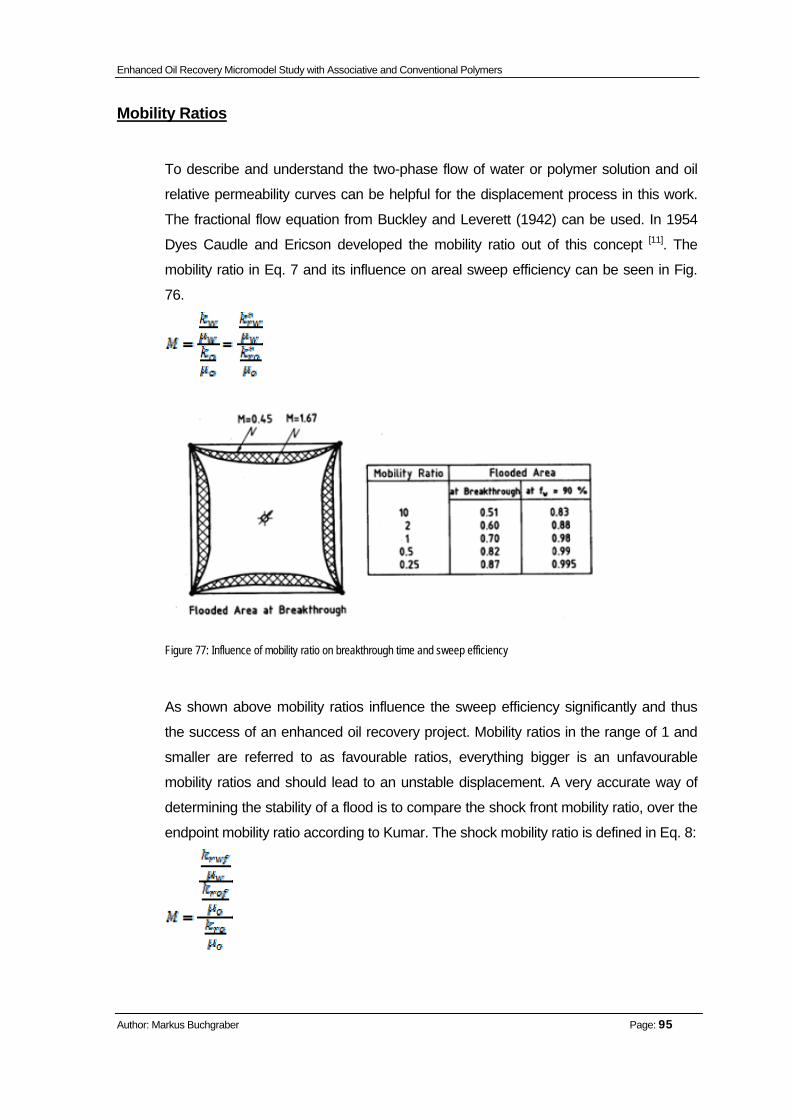
Enhanced Oil Recovery Micromodel Study with Associative and Conventional Polymers
Author: Markus Buchgraber Page: 95
Mobility Ratios
To describe and understand the two-phase flow of water or polymer solution and oil
relative permeability curves can be helpful for the displacement process in this work.
The fractional flow equation from Buckley and Leverett (1942) can be used. In 1954
Dyes Caudle and Ericson developed the mobility ratio out of this concept [11]. The
mobility ratio in Eq. 7 and its influence on areal sweep efficiency can be seen in Fig.
76.
Figure 77: Influence of mobility ratio on breakthrough time and sweep efficiency
As shown above mobility ratios influence the sweep efficiency significantly and thus
the success of an enhanced oil recovery project. Mobility ratios in the range of 1 and
smaller are referred to as favourable ratios, everything bigger is an unfavourable
mobility ratios and should lead to an unstable displacement. A very accurate way of
determining the stability of a flood is to compare the shock front mobility ratio, over the
endpoint mobility ratio according to Kumar. The shock mobility ratio is defined in Eq. 8:

Enhanced Oil Recovery Micromodel Study with Associative and Conventional Polymers
Author: Markus Buchgraber Page: 96
Due to the instability of the displacement front, the bank behind the front is not at the
endpoint mobility ratio[28]. For this work, only endpoint relative permeability values were
available and therefore Eq.7 was used to calculate mobility ratios for the different
experiments. Viscosity values for polymer solutions were obtained from Fig. 71 with a
shear rate of 0.09 sec-1. Mobility ratios for each experiment were calculated, assuming
that the relative permeabilities for polymer solution are equal to the water relative
permeability. Results are shown in Tab.14. Only ratios of the S255 could be calculated
due to missing data from the Alberta Research Council.
Concentration (ppm) Viscosity (cp) Mobility ratio
Brine 1 34.19
500 16.99 2.01
750 13 2.63
1000 11.8 2.90
1250 25.7 1.33
1500 35.39 0.97
2000 135 0.25
S255
2500 1004 0.03
Table 13: Mobility ratios for associative polymer solution and crude oil (450 cp)

Enhanced Oil Recovery Micromodel Study with Associative and Conventional Polymers
Author: Markus Buchgraber Page: 97
Permeability Reduction
Polymer plugging has been reported for a couple of experiments and can be useful as
well. In high permeable areas, which are almost completely water saturated, polymer
plugging can lead to a reduction of permeability and hence increase the flow
resistance so that the polymer slug will contact unswept areas. According to the
literature plugging only occurs when the polymer particle diameter is larger than a fifth
of the average pore diameter. In former micromodel experiments (Filiz Aktaz 2008) no
polymer plugging was reported neither by changed permeability nor by visual
observations. During these series of experiments, polymer plugging was observed by
incident at very low concentrations at the beginning. In order to determine the shear
rate in the MM, it has to be flooded with a polymer solution. The experimental steps of
this experiment are listed below:
• Saturate 100% with brine to determine permeability with Darcy´s law
• Saturate 100% with polymer solution
• Measure pressure drop at a constant flow rate
• Calculate viscosity
• Find corresponding shear rate according to Fig. 71
• Clean the micromodel with Toluen, Propanol and Water
• Saturate with brine to determine permeability
During the last step of this experiment a reduction in permeability was calculated
according to Darcy´s law, but the visual observation at micro scale did not show any
polymer plugging.
To obtain a better understanding of where the polymer particles plug the pores as well
as in which spatial distribution, the same experiment was done with a dyed polymer
solution. To colour the solution, two drops of conventional red food colour were added
to a 200 ml solution, Fig 78.
After the polymer flood, the same order of permeability reduction was observed and
additionally, the dyed solution showed its effects. The very first pore throats from the
inlet fraction side were obviously plugged with the polymers, as can be seen in Fig.
77. Plugging did not go further into the matrix, it was only within the first 10-15 pores.
Although after the experiment the MM was cleaned intensively with three different
cleaning fluids, according to the elutrope row (propanol-ethanol-water) to dissolve the

Enhanced Oil Recovery Micromodel Study with Associative and Conventional Polymers
Author: Markus Buchgraber Page: 98
polymer precipitation, the permeability measurements did not show any significant
changes. From Tab. 16 and Tab.17 below a permeability reduction from 1400 md to
933 md, which is almost 35%, can be seen.
As a measure of permeability reduction the residual resistance factor in Eq. 9 [11][8] can
be calculated, which is the mobility of a brine solution before(λ1) and after (λ1a)
polymer injection.
a
aaRf k
k
R
1
1
1
1
1
1
μ
μλλ
==
RRf is an indication of the permanence of the mobility reduction caused by the polymer
solution. It shows the quantity of channel and pore plugging and blocking of the
polymer solution. Another criteria of measurement the permeability reduction are the
resistance factor, which gives the ratio of injectivity of brine to that of single-phase
polymer solution which can be seen in Eq. 10
The fact that the polymer solution plugs pores and thus reduces permeability was of
major importance. Otherwise different experiments would have been done with the
same micromodel after cleaning without noticing that the permeability has changed.
As a logical fact, a new micromodel has to be used for every experiment in order to
guarantee repeatability.

Enhanced Oil Recovery Micromodel Study with Associative and Conventional Polymers
Author: Markus Buchgraber Page: 99
Figure 78: Polymer plugged (red) areas near inlet fracture of the micromodel
Figure 79: Dyed polymer solution with food colour
INPUT OUTPUT

Enhanced Oil Recovery Micromodel Study with Associative and Conventional Polymers
Author: Markus Buchgraber Page: 100
P2
(psig)
P2
(atm)
P1
(atm) >
Q
(mL/min)
Q
(mL/s)
Area
(cm^2) L (cm)
viscosit
y (cP) k (darcy)
28 2.90 1.00 0.4 0.0066 0.0125 5 1.0 1.4
21 2.43 1.00 0.3 0.005 0.0125 5 1.0 1.4
14 1.95 1.00 0.2 0.0033 0.0125 5 1.0 1.4
7 1.48 1.00 0.1 0.0016 0.0125 5 1.0 1.4
average 1.4
Table 14: Permeability measurements before injecting the polymer solution (measured with const. flow rate)
INPUT OUTPUT
P2
(psig)
P2
(atm)
P1
(atm) >
Q
(mL/min)
Q
(mL/s)
Area
(cm^2) L (cm)
viscosit
y (cP) k (darcy)
41 3.79 1.00 0.4 0.0066 0.0125 5 1.0 0.95
31 3.11 1.00 0.3 0.0055 0.0125 5 1.0 0.94
21 2.43 1.00 0.2 0.0033 0.0125 5 1.0 0.93
11 1.75 1.00 0.1 0.0016 0.0125 5 1.0 0.89
average 0.93
Table 15: Permeability measurement after injecting the polymer solution (measured with const. flow rate)

Enhanced Oil Recovery Micromodel Study with Associative and Conventional Polymers
Author: Markus Buchgraber Page: 101
Polymer Adsorption
Polymer adsorption is a major issue in polymer flooding. The changing polymer
characteristics and the concentration when the solution is flowing through the reservoir
and contacting rock and brine have to be observed. To determine if the polymer
solution changes after flooding through the micromodel, the following experiment was
done:
A polymer solution of associative polymer S255 with 2500 ppm was mixed and
viscosity versus shear rate was measured. Then, for 30 hours the micromodel was
flooded with the polymer solution at a constant pressure of 55 psi and at the outlets,
the polymer solution was gathered and measured again. This experiment does not
only show if any adsorption happened during the flood, but also if the polymer solution
was sheared too much to get damaged. The result can be seen in Fig. 79 and does
not indicate any changes in rheology.
Figure 80: Viscosity measurements before and after flooding the polymer solution through the micromodel
An intensive study of polymer adsorption was performed by Rousseau et al. in 2008.
They used silicon carbide granular packs with permeability and porosity of 1000±50

Enhanced Oil Recovery Micromodel Study with Associative and Conventional Polymers
Author: Markus Buchgraber Page: 102
md and 40±1 %. Two types of associative polymer and one conventional polymer
solution were tested. Mobility reduction reached a plateau for conventional polymers
with equivalent concentration, whereas the associative polymer solution increased the
mobility reduction and indicated an internal plugging trend. The determination of the
adsorbed layer thickness showed that associative polymer solution has a 7 times
higher thickness than conventional ones and corresponds to the amount of polymer
injected.
The adsorption phenomenon can either be assumed as a multi-layer adsorption or by
the adsorption of multi- chain aggregates already present in the polymer solution.
Further experiments showed that elevated salinities (58.4g/L NaCl) evolve to an over-
adsorption. Therefore, optimum salinity conditions have to be found for an associative
polymer solution flooding operation[29].

Enhanced Oil Recovery Micromodel Study with Associative and Conventional Polymers
Author: Markus Buchgraber Page: 103
Oil
The oil used for these experiments is dead oil from the Pirawath field in Austria. API
gravity and viscosities at reservoir conditions and at room temperature are measured.
To calculate API gravity, one litre of dead oil was weighed and the specific density
calculated and the index was determined with the API gravity formula as in Eq. 10.
The viscosity of the oil was measured with the DV-II-Pro+ Brookfield viscometer with a
thermal jacket. Measurements at room temperature and reservoir temperature can be
seen in Fig. 80 and Fig. 81
Figure 81: Oil viscosity measurements at room temperature (22.4°C)

Enhanced Oil Recovery Micromodel Study with Associative and Conventional Polymers
Author: Markus Buchgraber Page: 104
Figure 82: Oil viscosity measurements at reservoir temperature (30.0°C)

Enhanced Oil Recovery Micromodel Study with Associative and Conventional Polymers
Author: Markus Buchgraber Page: 105
Problems
A lot of problems occured before during and even after an experiment. Problems and
failures do not only cause only troubles, they also help to improve and show
weaknesses in the aperture and work flow of experiments. Accidents and human
failure often set back the work for a couple of days. Some of these problems and
accidents are reported in the section below to give a better understanding of
experimental work. Problems are listed in the chronological orders of an experimental
work flow
Drilling the entry and outlet ports
Drilling the holes for the fluid communication is one of the most serious tasks. A
damage of the wafer at this time would not only cost a lot of time, but also a lot of
money. The wafer has to be fixed with the fingers to drill the holes. Broken wafers
most often result from uneven pressure distribution during the fixing. Therefore, a very
flat and clean surface is required to drill the holes.
Bonding the wafer
The bonding process, described in one of the sections above is the last step of the
micromodel production. While the wafer is heated up for 50 minutes, very fine and tiny
particles can settle down on the top of the wafer. These small particles can cause a
bad bonding when the wafer is connected with the pyrex glass. The dust can be
removed before bonding with an air jet pump. Unfortunately, particles can melt
together with the wafer and cannot be removed, which most often makes the wafer
unusable.
Tighten micromodel in holder
Broken wafers also occur when tightening the micromodel holder. This happens when
the eight screws from the holder are not tightened star-shaped. By tightening them
clockwise or counter clockwise, the pressure is not distributed evenly and the wafer
may break. Another reason for a damaged wafer while tightening is probably a small
particle between holder and micromodel. This particle causes a stress point and
breaks the micromodel.

Enhanced Oil Recovery Micromodel Study with Associative and Conventional Polymers
Author: Markus Buchgraber Page: 106
Brine mixing
The brine mixing procedure requires a lot of time to avoid precipitation. Small particles
can plug the fine pores of the micromodel later on and give wrong results. Especially
Sodium Bicarbonate precipitates easily when mixing the brine. By adding it in small
portions within sufficient time intervals, this negative effect is avoided.
Polymer mixing and filtering
The polymer mixing is often insufficient and small undissolved polymer particles are
observed, which could result in a pore plugging. Therefore the mixing procedure is
usually done at slightly elevated temperatures of 30°C. Sometimes even the elevated
temperature is not sufficient in order to guarantee a smooth operation and therefore all
polymer solutions are filtered. To filter the solution, a cartridge filter with average filter
particle size of 15 μm was used. Viscosity measurements showed that the filter does
not change any properties or characteristics of the polymer solution.
Broken and leaking tubings
Broken or leaking tubings when noticed early enough are substituted by new ones and
the experiment is continued. But leaking or broken tubing during a flood cannot be
repaired or replaced fast enough in order not to falsify the experimental outcome.
Reason for a broken or leaking tubing is that the connection is tightened and screwed
many times. Leaking tubings can be identified by abnormal pump pressures or rates
during the experiment. Also, small drops on the surface of the desk can be a sign for
leaking tubings. Therefore, the cleaning of the desk before starting an experiment is
part of the workflow.
Air in tubings
Air bubbles in the tubings lead to wrong measurements and results. Most often air was
found in between the decane and brine vessel when saturating with brine. When
connecting and disconnecting the water pump to the decane vessel, small pockets of
air are trapped in the connection and flow into the vessel when pumping is started.
Trapped air causes wrong permeability measurements which in consequence lead to
the wrong assumption that the micromodel is not useable for the experiment. The
problem is solved by connecting a second valve to the decane vessel, where the air is
released when pumping starts.

Enhanced Oil Recovery Micromodel Study with Associative and Conventional Polymers
Author: Markus Buchgraber Page: 107
Connect tubings to micromodel
The connection from the oil vessel to the micromodel inlet port has to be tightened
very slowly. If tightened to fast, a high volume of oil is pushed into the micromodel in a
very short time and result in very high pressure. If the pressure exceeds a certain limit,
the micromodel will break. Therefore the connection is screwed very slowly and a very
low pressure of 5-10 psi is used to make the connection.
Photographs
The light and diffusion box has to be adjusted so that no shadows are visible when
taking meso scale pictures. At breakthrough time the micromodel holder has to be
taken to the microscope and micro scale pictures have to be taken in a time window of
2-3 min. Micro scale pictures after 5 or 10 minutes after breakthrough would result in a
wrong interpretation.
Image Analyses
Uneven illumination of the pictures makes them very difficult to be analysed. To
reduce the effect of illumination, only the middle part of the pictures is cut out and used
for further processing.

Enhanced Oil Recovery Micromodel Study with Associative and Conventional Polymers
Author: Markus Buchgraber Page: 108
Experimental Results and Discussions
A couple of experiments were conducted to observe the displacement of associative
polymer solution and to compare them with conventional polymer solution and brine
flood. An overview of the experiments is listed below.
• Brine Flood
• Associative Superpusher S255 (q=0.0001 ml/min) o 500 ppm
o 750 ppm
o 750 ppm (q=0.0004 ml/min)
o 1000 ppm
o 1250 ppm
o 1500 ppm
o 3x 2500 ppm (to prove the almost complete plugging of pores at this
high concentration)
• Conventional FP3630 (q=0.0001 ml/min) o 500 ppm
o 750 ppm
o 750 ppm (q=0.0003 ml/min)
o 1000 ppm
o 1250 ppm
o 1500 ppm
• Brine- Polymer Combination (Switch to S255 2000 ppm after BT)
• Brine- Polymer Combination (Switch to S255 2000 ppm after 2/3 of BT)
• Brine- Polymer Combination (Switch to S255 1750 ppm after 1/2 of BT)
• Brine- Polymer Combination (Switch to S255 1500 ppm after 22 hours
brine flood)
All experiments except the combination ones, had the same flow rate of 0.0001
ml/min, which refers to 12 cm/day. The oil, which was described before, was
intermediate oil from the Pirawath field in Austria. Care had to be taken to have the
same initial conditions before starting each experiment. Temperature, mixing time and
quality of polymer and permeability variations in the micromodel have to be checked
before starting. All experiments had an initial water saturation between 2% and 10%.

Enhanced Oil Recovery Micromodel Study with Associative and Conventional Polymers
Author: Markus Buchgraber Page: 109
A 22.4°C room temperature was measured for all experiments. Experimental data
gathering sheets had been laid out for each experiment, which included saturation
times for water and oil, permeability measurements and pressure measurements
during the flood experiments. An example of such an data sheet from a 500 ppm
polymer flood can be seen in Appendix C.
Brine Flood The baseline for all later experiments was the brine flood done at the very beginning of
the study. As expected, the brine flood showed a very serious fingering behaviour in
the middle of the micromodel which grew till it reached the outlet fracture and caused
the breakthrough after 71 min.
A closer look at Fig. 82 shows another finger at the edge of the micromodel. This
effect was observed many times later on. In some cases these edge fingers caused
the breakthrough. The origin of the effect is unknown, but it is assumed to be a
bonding effect, because the weight is only applied in the middle of the glass plate. So
the outer parts may have less bonding and therefore less resistance to flow.
Further flooding also showed that after 22 hours some areas of the micromodel stayed
unswept. The result was the same as predicted in literature: early breakthrough, with a
lot of bypassed oil and after a long flooding period still un-contacted areas. Another
evidence of the unstable displacement was the calculated mobility ratio of Tab. 14.
Fig. 82 shows the sequence of the flood till breakthrough and the final picture after 22
hours.
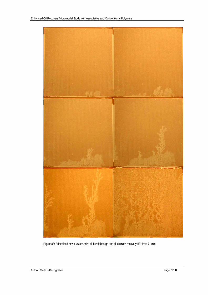
Enhanced Oil Recovery Micromodel Study with Associative and Conventional Polymers
Author: Markus Buchgraber Page: 110
Figure 83: Brine flood meso scale series till breakthrough and till ultimate recovery BT-time: 71 min.

Enhanced Oil Recovery Micromodel Study with Associative and Conventional Polymers
Author: Markus Buchgraber Page: 111
Associative Polymer Floods All the experiments discribed in this part were made with the associative polymer
Superpusher 255. The recovery at breakthrough ranges from 9.4% to 38.8%.
Breakthrough times did not show any relation to recovery. The first polymer solution
flood was at 500 ppm. The concentration was stepwise increased by 250 ppm till a
more or less stable displacement was observed. Better sweep efficiency and therefore
recovery at the same concentration as the conventional polymers are the expectations
of these new polymers. All the following pictures present the displacement process in
meso scale till breakthrough (first picture in third row) and till ultimate recovery (second
picture in third row).
The 500 ppm solution shows similar behaviour as the brine displacement. Very early
in the flood, two dominant fingers developed, which broke through after 51 min. In
contrast to the brine flood, some smaller fingers developed as well which started
growing more intensively after the breakthrough. Most of the fingers start merging at
half way and build a more cloudy shape of displacement front towards the outlet
fracture. After 22 hours of flood, a second front which came up only 10-15 mm into the
micromodel matrix can be seen at the beginning of the inlet fracture. This brighter area
has a better micro sweep efficiency than the other swept regions. Only very small
spots of unswept areas were observed during this flood. No improvement of recovery
at breakthrough compared to the brine flood could be achieved. Fig. 83 shows meso
scale pictures till breakthrough and after 22 hours.
The 750 ppm polymer solution had a breakthrough after 50 min. Finger development
was almost the same as for the 500 ppm solution. The only difference was that the
breakthrough fingers were not predominant. At BT a lot of fingers were already
merged and swept a large part of the micromodel. The size and shape of the fingers
were the same as in the previous experiment. See Fig. 84. In addition, an experiment
with the same polymer concentration with a changed flow rate was conducted in order
to observe the influence of changed flow rates on displacement. The elevated flow
rate of 0.0004 ml/min or 50 cm/day did not show any significant changes in recovery
or swept area.

Enhanced Oil Recovery Micromodel Study with Associative and Conventional Polymers
Author: Markus Buchgraber Page: 112
1000 ppm of polymer in solution showed the first slight improvements in stable
displacement. No dominant single fingers grew early in flood life. A lot of small short
fingers developed at the beginning, followed by a thin stable front of polymer solution.
Although fingers became bigger later on, the polymer front behind did not stop, see
Fig. 85. A couple of even fingers at almost the same height caused the breakthrough.
Recovery factor and swept area at breakthrough could be significantly improved.
The experiment with best recovery and swept area after breakthrough proved to be
the one with a 1250 ppm polymer solution. From the beginning, a very continuous
stable front moved towards the outlet fracture. Only very small, skeletal and short
fingers were visible ahead of the front. Finger number and length also decreased with
increasing concentration, as can be seen in Fig.86. The breakthrough was caused by
a finger at the edge after 91 min.
To prove whether this stable front was a lucky incident or a success of the polymer
solution, the concentration was increased for another 250 ppm to a 1500 ppm polymer
solution. The results were even better at the beginning than those at 1250 ppm, as a
consequence of the more stable mobility ratio. Unfortunately the breakthrough was
caused by a finger at the edge of the micromodel. Till half way, the displacement was
perfectly stable as indicated in Fig. 87, even the very small fine fingers ahead of the
front can be distinguished. Without the breakthrough at the edge this flood would have
been more successful in terms of recovery factor and sweep efficiency.
The last experiment with the associative polymer solution was done at a concentration
of 2500 ppm. The aim of this run was to observe if there is a concentration limit, at
which the polymer solution plugs the pores too much and hence causes poor recovery
and sweep efficiency. In fact the first run showed a perfectly stable displacement till
half way of breakthrough. No viscous fingers were seen a head of the front instead a
cloudy front developed. Breakthrough was again caused by an edge finger, Fig. 88.
After breakthrough the polymer solution was not able to sweep the whole area and left
a lot of bypassed oil behind. This could be a consequence of the too high
concentration. A second run with the same concentration was conducted to repeat the
behaviour. And again the same plugging occurred with a lot of bypassed oil after 22
hours of flooding.

Enhanced Oil Recovery Micromodel Study with Associative and Conventional Polymers
Author: Markus Buchgraber Page: 113
Figure 84: Associative polymer flood S255, 500 ppm; BT-time: 51 min.
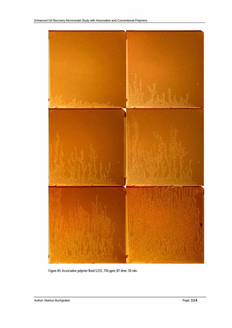
Enhanced Oil Recovery Micromodel Study with Associative and Conventional Polymers
Author: Markus Buchgraber Page: 114
Figure 85: Associative polymer flood S255, 750 ppm; BT-time: 50 min.

Enhanced Oil Recovery Micromodel Study with Associative and Conventional Polymers
Author: Markus Buchgraber Page: 115
Figure 86: Associative polymer flood S255, 1000 ppm; BT-time: 91 min.

Enhanced Oil Recovery Micromodel Study with Associative and Conventional Polymers
Author: Markus Buchgraber Page: 116
Figure 87: Associative polymer flood S255, 1250 ppm; BT-time: 107 min.

Enhanced Oil Recovery Micromodel Study with Associative and Conventional Polymers
Author: Markus Buchgraber Page: 117
Figure 88: Associative polymer flood S255, 1500 ppm; BT-time: 64 min.
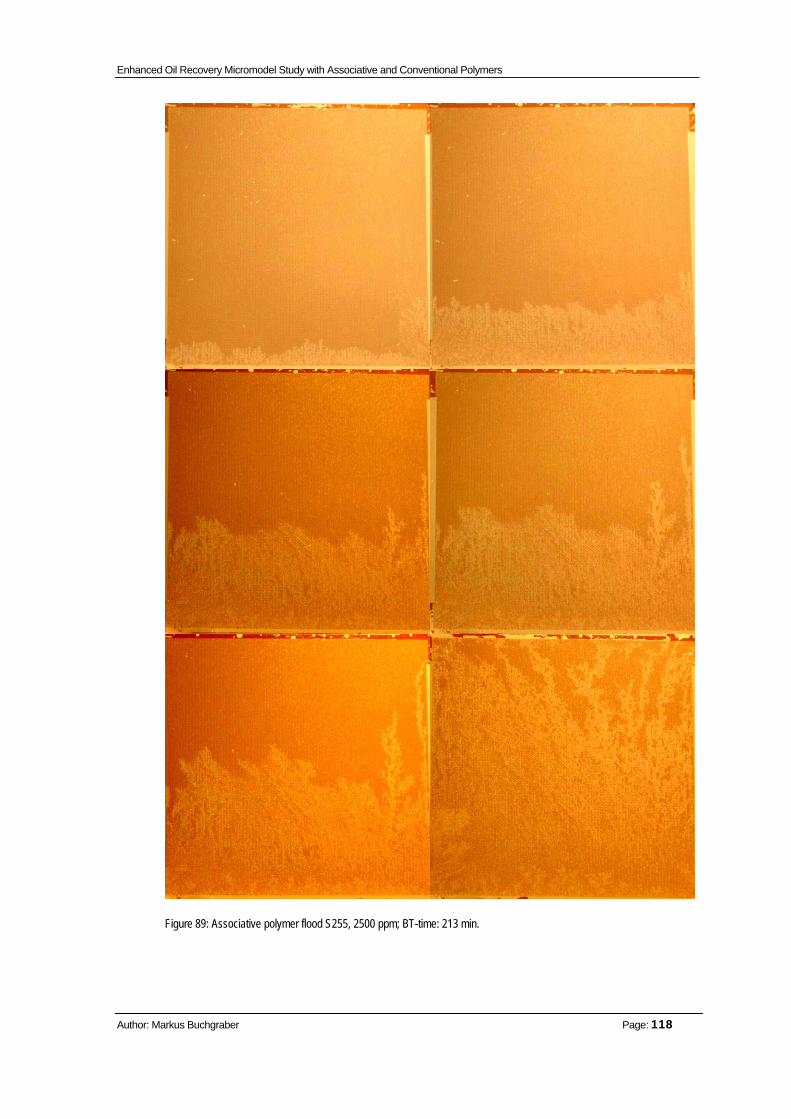
Enhanced Oil Recovery Micromodel Study with Associative and Conventional Polymers
Author: Markus Buchgraber Page: 118
Figure 89: Associative polymer flood S255, 2500 ppm; BT-time: 213 min.

Enhanced Oil Recovery Micromodel Study with Associative and Conventional Polymers
Author: Markus Buchgraber Page: 119
Conventional Polymer Floods
The same series of experiments was performed with the conventional polymer. As a
starting concentration a 500 ppm polymer solution was used. Breakthrough times
were completely different and allowed no possible relation to recovery or sweep
efficiency.
500 ppm solution of the conventional solution showed a similar behaviour as the
associative with the only difference that the shape of the fingers had changed. Fingers
appeared thinner and finer and merged at an earlier stage, Fig.89.
The 750 ppm solution had several fingers and additionally led to a breakthrough at 25
min. As observed in the earlier experiments the fingers started merging together and
building small displacement fronts behind them. Fig. 90 shows the displacement till
ultimate recovery of the 750 ppm solution. An elevated flow rate was used to observe
the influence on different flow rates. But the 0.0004 ml/min did not show any significant
success or failure.
An improved performance could be observed at the 1000 ppm solution. Fingers were
at the same height when moving towards the outlet end. The displacement cannot be
referred to as stable, but the trend to a stable displacement can be seen in Fig.91.
The best performance again when considering the edge fingers is the 1250 ppm
solution. Micro scale saturation pictures and meso scale sweep efficiency were by far
the highest at this solution. At breakthrough time the fingers completely merged to a
front and showed an almost stable displacement, which can be seen in Fig 92.
The last experiment was conducted with the 1500 ppm solution and did not increase
recovery or sweep efficiency from the 1250 ppm solution (Fig. 93).

Enhanced Oil Recovery Micromodel Study with Associative and Conventional Polymers
Author: Markus Buchgraber Page: 120
Figure 90: Conventional polymer flood FP3630, 500 ppm; BT-time: 25 min.

Enhanced Oil Recovery Micromodel Study with Associative and Conventional Polymers
Author: Markus Buchgraber Page: 121
Figure 91: Conventional polymer flood FP3630, 750 ppm; BT-time: 81 min.

Enhanced Oil Recovery Micromodel Study with Associative and Conventional Polymers
Author: Markus Buchgraber Page: 122
Figure 92:Conventional polymer flood FP3630, 1000 ppm; BT-time: 17 min.

Enhanced Oil Recovery Micromodel Study with Associative and Conventional Polymers
Author: Markus Buchgraber Page: 123
Figure 93: Conventional polymer flood FP3630, 1250 ppm; BT-time: 28 min.

Enhanced Oil Recovery Micromodel Study with Associative and Conventional Polymers
Author: Markus Buchgraber Page: 124
Figure 94: Conventional polymer flood FP3630, 1500 ppm; BT-time: 25 min.

Enhanced Oil Recovery Micromodel Study with Associative and Conventional Polymers
Author: Markus Buchgraber Page: 125
Brine Associative Superpusher 255
Concentration (ppm) 500 750 1000 1250 1500 2500
Permeability (md) 1311 905 1075 980 1160 1370 1422
BT-time (min) 71 51 50 91 107 64 213
Pore volume injected (ml) 0.54 0.39 0.38 0.69 0.81 0.48 1.61
BT-recovery (%) 17.6 16.9 21.4 27.9 38.8 30.4 9.43
22 hours recovery (%) 34.4 39.9 41.3 37.9 40.3 35.5 25.2
Table 16: Results for brine- and associative polymer flood experiments
Brine Conventional FP 3630
Concentration (ppm) 500 750 1000 1250 1500
Permeability (md) 1311 1427 1151 1350 1200 1150
BT-time (min) 71 25 81 17 28 25
Pore volume injected (ml) 0.54 0.19 0.61 0.13 0.21 0.19
BT-recovery (%) 17.6 16.9 22.0 29.9 31.2 38.0
22 hours recovery (%) 34.4 37.4 34.5 31.5 33.8 36.5
Table 17: : Results for brine- and conventional polymer flood experiments

Enhanced Oil Recovery Micromodel Study with Associative and Conventional Polymers
Author: Markus Buchgraber Page: 126
Finger Analysis and Sweep Efficiency
Finger analysis consists of the measurement of length and number of obvious fingers.
The finger length was measured from the base line or from an average advancement
of the front and was determined visually. Not every single finger is counted in this
analysis. Only those which were easily detectable were taken into account.
An example of counted and measured fingers with a base line can be seen in Fig 94.
This example below is from the breakthrough time of the 500 ppm conventional
polymer solution. With increasing concentration, the number of fingers decreased as a
consequence of the decreased mobility ratio. Finger length at a higher concentration
which was caused by the edge fingers has to be taken with care when making further
conclusions. But the general trend that the 1250 ppm and 1500 ppm polymer solution
gave the best results with respect to the edge fingers can be seen in the following
charts (Fig. 95 to Fig. 98) as well.
Figure 95: Meso scale photograph at breakthrough with finger base line and counted fingers

Enhanced Oil Recovery Micromodel Study with Associative and Conventional Polymers
Author: Markus Buchgraber Page: 127
Figure 96: Effect of increasing concentration on finger number for conventional polymer
Figure 97: Dependency of finger length on polymer concentration for conventional polymer

Enhanced Oil Recovery Micromodel Study with Associative and Conventional Polymers
Author: Markus Buchgraber Page: 128
Figure 98: Effect of increasing concentration on finger number for associative polymer
Figure 99: Dependency of finger length on polymer concentration for associative polymer

Enhanced Oil Recovery Micromodel Study with Associative and Conventional Polymers
Author: Markus Buchgraber Page: 129
Swept Areas
Based on the meso scale photographs, the swept area at breakthrough time was
determined. The similarity of swept and unswept areas made it impossible to process
the picture with the computer. Hence, swept areas had to be marked manually
,because of the low colour contrast of the picture. Sweep efficiency was determined
with G.I.M.P. image analyses procedure. Figure 99 to Fig. 101 below present the
swept areas in black and the unswept in white after being processed from associative
and conventional polymer solutions.
Figure 100: Swept areas for conventional and associative polymer solution
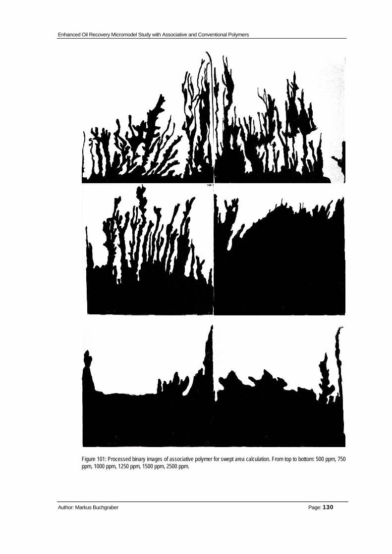
Enhanced Oil Recovery Micromodel Study with Associative and Conventional Polymers
Author: Markus Buchgraber Page: 130
Figure 101: Processed binary images of associative polymer for swept area calculation. From top to bottom: 500 ppm, 750 ppm, 1000 ppm, 1250 ppm, 1500 ppm, 2500 ppm.

Enhanced Oil Recovery Micromodel Study with Associative and Conventional Polymers
Author: Markus Buchgraber Page: 131
Figure 102: Processed binary images of conventional polymer for swept area calculation. From top to bottom: 500 ppm, 750 ppm, 1000 ppm, 1250 ppm, 1500 ppm
Enhanced Oil Recovery Micromodel Study with Associative and Conventional Polymers
Author: Markus Buchgraber Page: 132
Combination Flood Experiment The experiments mentioned above had the goal to find a polymer concentration which
lead to a stable displacement. The cases in which a polymerflood is conducted in the
secondary recovery stage are very rare. Normally polymer floods are started at tertiary
recovery stage, when an intensive waterflood has already been done and water has
already broken through. In this case a polymer solution is used to reduce the
permeability of high velocity paths and contacts the bypassed oil. Consequently, the
water production should be reduced and more oil produced.
In the micromodel it is not possible to wait for a waterflood breakthrough and then
switch to the polymer solution to observe the above effect. Dimensions in the model
are too small and it often takes less than 5-10 minutes, from breakthrough to a total
swept area which is the time needed to switch from water to a polymer solution. First
experiments were done in the way described above, but it was not observable if the
fingers could be reduced after injecting the polymer solution.
So the further approach was to flood with water till half or a third of breakthrough and
then switch to the polymer solution. The results showed a very positive effect of the
associative polymers. The fingers developed initially had been smoothed by the
polymer solution. Because of the very small contrast the changing front is marked with
a black pen see Fig. 103. So, this result leads to the assumption that an initiation of a
polymer flood after a water breakthrough can decrease the viscous fingering and
therefore contact more areas in the reservoir which results in increased recovery.

Enhanced Oil Recovery Micromodel Study with Associative and Conventional Polymers
Author: Markus Buchgraber Page: 133

Enhanced Oil Recovery Micromodel Study with Associative and Conventional Polymers
Author: Markus Buchgraber Page: 134
Figure 103: Combination flood. Switch from brine injection to polymer solution at picture 5 (third row second picture)

Enhanced Oil Recovery Micromodel Study with Associative and Conventional Polymers
Author: Markus Buchgraber Page: 135
Residual Oil Recovery Experiment This experiment was done with the purpose to investigate if the injection of a polymer
solution can reduce the residual oil saturation. To observe this effect, the oil saturated
micromodel was first flooded with water for 22 hours. After 22 hours no more oil
production resulted from injecting more water.
At this time the brine vessel was disconnected, micro scale pictures were taken to
determine the oil saturation and the polymer solution was injected into the
micromodel. The flood was continued for a second 22 hour period. Finally pictures
were taken and oil saturation was determined.
The comparison of the image analyses showed no additional oil production after the
polymer injection.
Enhanced Oil Recovery Micromodel Study with Associative and Conventional Polymers
Author: Markus Buchgraber Page: 136
Conclusions
The aim of this study was to observe the displacement process of polymer solutions.
During the experiments, augmented associative and conventional polymers with
different concentrations ranging from 500 ppm to 2500 ppm were used. Oil recoveries
and sweep efficiencies were obtained by taking high resolution photographs at meso
and macro scale and processing them further. Almost unchanged initial conditions and
very careful experimental work led to reliable results. In addition to the conventional
floods, combination floods had been conducted. The reason was to observe the
effects of decreasing viscous fingers and the recovery of residual oil by polymer
injection. This study reports experimental results showing that:
• Conventional brine flood with an unfavourable mobility ratio showed serious
viscous fingers causing an early breakthrough and therefore poor sweep
efficiency and recovery factor.
• By increasing the concentration stepwise the sweep efficiency at the
breakthrough could be improved for associative and conventional polymer
solutions. In some experiments an edge finger evolved, which probably
caused an early breakthrough.
• Increased polymer concentration of associative and conventional polymers
also led to a better recovery factor at breakthrough time.
• Sweep efficiency and recovery indicate that a polymer concentration of 1250
ppm (M=1.33) to 1500 ppm (M=0.97) led to the best results for the described
conditions and fluids.
• The finger analysis also demonstrated a decreasing finger number and length
with an increasing concentration.
• A stable displacement in the presence of only minor viscous fingers could only
be observed for associative polymer solutions. A conventional polymer
solution indicated viscous fingers for all used concentrations. Fingers of the

Enhanced Oil Recovery Micromodel Study with Associative and Conventional Polymers
Author: Markus Buchgraber Page: 137
two polymer types differ in appearance and interval. Conventional polymer
flood fingers seemed to be more tiny and closer together and merged towards
the outlet fracture, whereas associative fingers tented to build thicker single
fingers and to merge at a later stage of the flood.
• An associative polymer concentration of 2500 ppm led to a poor recovery and
sweep efficiency. It was assumed that this concentration was too high and
caused a very serious pore plugging by multi-layer polymer adsorption.
• No relation between ultimate recovery after flooding ten pore volumes and
polymer concentration for both polymer types could be observed and
measured.
• Already developed and advancing fingers could be thickened and even
smoothed by the injection of an associative polymer solution.
• By the injection of an associative polymer solution after reaching the ultimate
recovery with a water flood, no additional oil could be recovered, meaning that
polymer flooding operations cannot recover any residual oil.
• Associative polymer solutions did not show any significant higher recoveries
and swept areas at breakthrough than conventional polymers. However stable
displacement was only obtained by an associative polymer solution.
• A residual resistance factor, RRf , of 1.5 was measured in an experiment. This
value fits to other measured core experiments in literature.

Enhanced Oil Recovery Micromodel Study with Associative and Conventional Polymers
Author: Markus Buchgraber Page: 138
Follow up
As a follow-up of this study, multiple repeated experiments should be conducted in
order to determine to what degree standardization of initial conditions, and additionally
to what degree varying the input parameters (i.e. viscosity and flow rate) can affect the
anatomy of the displacement front. Further experiments with real cores investigating
the polymer adsorption effect and polymer plugging would be of importance.
Additionally computer tomography pictures analysing the saturations at different
positions and times in the micromodel would enable the comparison to simulation
programs.
Future experimets

Enhanced Oil Recovery Micromodel Study with Associative and Conventional Polymers
Author: Markus Buchgraber Page: 139
References
1. R.Jennings et al. “Factors Influencing Mobility Control by Polymer Solutions”, SPE
2867, JPT Volume 23, (March1971)
2. Manning, R.K et al.:” Technical survey of polymer flooding projects”, Report
DOE/ET/10327-19, (Sept.1983)
3. Forrest F. Craig Jr.: The reservoir engineering aspect of waterfloods, Monograph
SPE
4. Van Meurs P. “The use of transparent Three-Dimensional Models for studying the
mechanism of Flow processes in oil reservoirs”, SPE 000678, Trans., AIME 295-301,
(1957)
5. BENHAM, A.L.” A model study of viscous fingers” SPE 513, (Juni 1963)
6. Saffman P.G. and Taylor G. I.,” The penetration of fluid into a porous medium or
hele-shaw cell containing a more viscous liquid”, Proc. Royal society London Vol.213,
103-112, (1958)
7. Van Meurs P. and van der Poel C.” A theoretical description of water drive
processes involving viscous fingers”, Trans, AIME, Vol. 213, Pages 103-112 SPE
000931, (1953)
8. W. Littmann, “Polymer flooding” ISBN 0-444-43001-6
9. Y. Du et al.: “Field-scale Polymer Flooding: Lessons Learned and Experiences
Gained During Past 40 Years”, SPE 91787, (2004)
10. R.D. Kaminsky et al.:”Guidelines for polymerflooding Evaluation and Development”
SPE 11200, (2007)
11. Jerry W. Lake, Enhanced Oil Recovery, ISBN 0-13-281601-6

Enhanced Oil Recovery Micromodel Study with Associative and Conventional Polymers
Author: Markus Buchgraber Page: 140
12. Mojdeh Delshad et al.:” Mechanistic Interpretation and Utilization of Viscoelastic
Behaviour of Polymer Solutions for Improved Polymer-Flood Efficiency”, SPE/DOE
113620, (2008)
13. M, Pancharoen et al.:” Physical Properties of Associative Polymer Solutions “,
SUPRI-A Stanford University Petroleum Research Institute Thirty-first Annual
Report, (2008)
14. www.merriam-webster.com
15. www.brookfieldengineering.com/education/what-is-viscosity.asp
16. Sarah Inwood, “High Resolution, Microvisual Study of High Mobility Ratio,
Immiscible Displacement”, Stanford University, Master Thesis 2008,
17. Ashwini A. Upadhyaya,” Visualization of Four-Phase Flowing Using Micromodels”,
Stanford University, Master Thesis 2001.
18. Mattax, C.C. and Kyte, J.R.: “Ever see a Water Flood”, Oil and Gas Journal 115-
128, (Oct. 1961)
19. Davis Jr., J.A. and Jones, S.C.: “Displacement Mechanisms of Micellar
Solutions,” JPT, SPE-1847, (Dec. 1968)
20. Owete, O.S. and Brigham, W.E.: “Flow Behaviours of Foam: A Porous
Micromodel Study,” SPERE 315-323, (Aug 1987)
21. Hornbrook, J.W., Castanier, L.M. and Petit, P.A.: “Observation of Foam/Oil
Interactions in a New, High-Resolution Micromodel,” SPE 22631,(Oct. 1991)
22. Keller, A.A., Blunt, M.J. and Roberts, P.V.: “Micromodel Observation of the
Role of Oil Layers in Three-Phase Flow,” Transport in Porous Media 26,
277-297, (1997)
23. Bruce T. Campbell. and Orr, F.M.: “Flow Visualization for CO2/Crude-Oil

Enhanced Oil Recovery Micromodel Study with Associative and Conventional Polymers
Author: Markus Buchgraber Page: 141
Displacements,” SPEJ 665-678, (Oct. 1985).
24. George, D.S.: “Visualization of Solution Gas Drive in Viscous Oil”, Stanford
University, Master Thesis 1999
25. Aktaz Filiz,” The Reservoir Behaviour of Associative Polymers”, Stanford
University a. University Leoben, Master Thesis 2007
26. OMV, Alberta Research Council
27. SNF Floerger Technical Data Sheet
28. Mridul Kumar et al.:”High-Mobility-Ratio Waterflood Performance Prediction:
Challenges and New Insights”, SPERE 186-196, SPE 97671, (Feb. 2008)
29. D. Rousseau et. Al.:”Associative Polymers for EOR - Towards a Better
Understanding and Control of Their Adsorption in Porous Media”, EAGE, (June 2008)
30. http://snf.stanford.edu/Equipment/EquipByName.html

Enhanced Oil Recovery Micromodel Study with Associative and Conventional Polymers
Author: Markus Buchgraber Page: 142
Nomenclature
φ Porosity [%]
μ Viscosity [cp]
λ1a Mobilty of brine after polymer flood [ ]
λ1 Mobility of brine [ ]
λ1´ Mobilty of single phase polymer [ ]
A Area [cm²]
dl Length [cm]
dp Pressure [bar]
dx Length [cm]
F Force [N]
F´ Shear Rate [sec-1]
fo Fractional Flow of oil [ ]
fw Fractional flow of water [ ]
kro Relative permeability of oil [ ]
kro* Endpoint relative permeability of oil [ ]
krw Relative permeability of water [ ]
krw* Endpoint relative permeability of water [ ]
M Mobilty ratio [ ]
no Oil exponent for saturation calculation [ ]
nw Water exponent for saturation calculation [ ]
Np Cumulative production [bbl/day]
npl Fluid coefficient [ ]
q Flow rate[m³/day]
RRf Residual resistance factor [ ]
S Shear stress [N]
Sbtp Saturation at polymer breakthrough [%]
Sbtw Saturation at water breakthrough [%]
Sor Residual oil saturation [%]
Spf Saturation at the polymer front [%]
Swf Saturation at the water front [%]
Swi Initial water saturation [%]
Swor Water saturation at residual oil saturation [%]
Swr Connate water saturation [%]
u Superficial velocity [cm/sec]
v Velocity[cm/sec]
Wi Injected pore volume [bbl/day]

Enhanced Oil Recovery Micromodel Study with Associative and Conventional Polymers
Author: Markus Buchgraber Page: 143
Appendix
Appendix A
The Etching Process
The Etching process is done completely in the SNF and requires special training and
equipment. Below all the equipment and machines which are used during this process
are listed and introduced according to the production process from the beginning to
the end[30].
Silicide Wet Bench
The Silicide Wet Bench is used for the cleaning of 3" or 4" silicon or SiGe wafers.
Wafers containing Tungsten or Titanium silicides, but no other metals, may be
processed here. This station contains sulfuric/peroxide hot pots, an HCl hot pot, and
HF tanks in addition to dump rinse and spin-rinse-dry modules. The available chemical
baths are:
• 90% Sulfuric Acid/Hydrogen Peroxide ("piranha") for resist strip
• 4:1 Sulfuric Acid:Hydrogen Peroxide for removal of trace organics
• 5:1:1 H2O:H2O2:HCl for removal of trace metal ions
• 50:1 HF, for oxide etching
• 6:1 BOE for oxide etching[30]

Enhanced Oil Recovery Micromodel Study with Associative and Conventional Polymers
Author: Markus Buchgraber Page: 144
SVG Photoresist Spin Coater
The SVG (Silicon Valley Group) coater is an automated track system for dispensing
photoresist on 4" silicon, glass, or quartz wafers. The system includes three stations: a
prime oven which bakes the wafer and dispenses the adhesion promoter, HMDS; and
a combination spinner, which dispenses photoresist, and a pre-bake oven which cures
the resist. The uniformity of spun photoresists are typically +/- 100 Å[30].
Figure 104: Photoresist Coater[30]
Karl Suss- Exposing
The Karl Suss MA-6 Contact Aligner system can perform precision mask-to-wafer
front- or back-side alignment and near-UV photoresist exposure in any one of three
modes (hard- and soft- contact, and high and low vacuum contact). The current
configuration accomodates 3" and 4" wafers and pieces. SNF has two MA-6
aligners[30].
SVG Developer
The SVG (Silicon Valley Group) developer is an automated system with two
independent tracks for developing and post-baking exposed photoresist-coated 4"
wafers. Each track system includes two stations: a spin station which dispenses and
rinses away developer; and an oven station for post-bake[30].

Enhanced Oil Recovery Micromodel Study with Associative and Conventional Polymers
Author: Markus Buchgraber Page: 145
Figure 105: Developing machine-chemical Wash[30]
STS Deep RIE Etcher
The STS etcher is used to remove specific parts of the resist or wafer.CF3+ and F act
as the etching gases. Oxide or photoresist may be used for mask.
Etches up to 6 µm/minute.
Metals may not be used as an etch mask, though they can be used as a mask stop
Au, Cr, Ni, and magnetics are never allowed in the machine[30].
Figure 106: STS-Etching machine with control computer[30]
ZYGO White-Light 3D Surface Profiler
The Zygo White-Light 3D Surface Profiler provides fast, non-destructive, quantitative
surface characterization of step heights, texture, roughness, and other surface
topography parameters. The measurement technique is non-contact, three-
dimensional, scanning white light and optical phase-shifting interferometry[30].

Enhanced Oil Recovery Micromodel Study with Associative and Conventional Polymers
Author: Markus Buchgraber Page: 146
The Zygo is based on scanning white-light interferometry, a traditional technique in
which a pattern of bright and dark lines (fringes) result from an optical path difference
between a reference and a sample beam. Incoming light is split inside an
interferometer, one beam going to an internal reference surface and the other to your
sample. After reflection, the beams recombine inside the interferometer, undergoing
constructive and destructive interference and producing the light and dark fringe
pattern.
Available objectives are: 2.5X, 10X, 20X, and 50X with additional zoom from 0.5 to 2X
Field of view ranges from 0.14 x 0.11mm (50X) to 2.82 x 2.11mm (2.5X)
Vertical resolution is 0.1 nm
Minimum lateral resolution is 0.22 µm (50X objective, 2X zoom) [30]
Figure 107: Zygo-electron microscope[30]

Enhanced Oil Recovery Micromodel Study with Associative and Conventional Polymers
Author: Markus Buchgraber Page: 147
Appendix B MATHLAB Routine function average=zoom(dirname)
black=0;
white=0;
schnittwhite=0;
schnittblack=0;
averagewhite=0;
averageblack=0;
summe=0;
cd(dirname)
names=dir('*.JPG');
nnames=length(names);
prozent=zeros(nnames,1);
oil=zeros(nnames,1);
for i=1:nnames
fname=names(i).name
X =imread(fname);
X=imcrop(X,[400 250 3200 2500]);
A =X;
for m=1:2500
for n=1:3200
indi=0;
black2=0;
if ((X(m,n,1)>79) && (X(m,n,2)>108) && (X(m,n,3)>80))
white=white+1;
X(m,n,1)=250;
X(m,n,2)=250;
X(m,n,3)=250;
indi=1;
else
black=black+1;
X(m,n,1)=0;
X(m,n,2)=0;
X(m,n,3)=0;
Enhanced Oil Recovery Micromodel Study with Associative and Conventional Polymers
Author: Markus Buchgraber Page: 148
end
end
end
datei=['blackwhite' fname ];
imwrite(X,datei,'jpg');
white=white/80000
black=black/80000
imshow(X);
schnittblack=schnittblack+black;
schnittwhite=schnittwhite+white;
summe=0;
oil(i)=black-26.00;
black=0;
white=0;
pause
end
averagewhite =schnittwhite/nnames
averageblack =schnittblack/nnames
oil

Enhanced Oil Recovery Micromodel Study with Associative and Conventional Polymers
Author: Markus Buchgraber Page: 149
Appendix C
Experimentnr.:13 Date: 12/03/2008 MMnr.:
m9(01/03/2008)
# of experiments with same MM: 1
Description: Associative Polymerflood with S255 (500 ppm)
Oil(name/μ): OMV Flooding fluid(name/ppm/μ): S255; 500ppm
200 g brine
0.1 g S255
Flow test: const. pressure & const. flow rate
INPUT OUTPUT
P2
(psig)
P2
(atm)
P1
(atm)
Q
(mL/min)
Q
(mL/s)
Area
(cm^2) L (cm)
viscosity
(cP) k (darcy)
40 3.72 1.00 0.378 0.0063 0.0125 5 1.0 0.9261
30 3.04 1.00 0.277 0.0046 0.0125 5 1.0 0.9047
20 2.36 1.00 0.179 0.0029 0.0125 5 1.0 0.8771
10 1.68 1.00 0.088 0.0014 0.0125 5 1.0 0.8624
average 0.89267
INPUT OUTPUT
P2
(psig)
P2
(atm)
P1
(atm) >
Q
(mL/min)
Q
(mL/s)
Area
(cm^2) L (cm)
viscosity
(cP) k(darcy)
37 3.2 1.0 0.35 0.0058 0.0125 5 1.0 0.92707
32 3.18 1.00 0.3 0.005 0.0125 5 1.0 0.91875
21 2.43 1.00 0.2 0.0033 0.0125 5 1.0 0.93333
11 1.75 1.00 0.1 0.0016 0.0125 5 1.0 0.89099
average 0.91755
Calculated perm.: 905 md
Cleaning: CO2
Brine saturation:
Starttime: 10.55 Startvol.: 74.00 ml Vol. inject.: 14.00ml
Endtime: 11.55 Endvol.: 60.00 ml

Enhanced Oil Recovery Micromodel Study with Associative and Conventional Polymers
Author: Markus Buchgraber Page: 150
Oil saturation:
Starttime: 12.00 Startvol.: 59.9 ml Vol. inject.: 0.5ml
Endtime: 20.20 Endvol.: 59.4 ml
Micro scale pictures were taken after every hour to investigate how the saturation
changes after time
Image analysis results assuming 22.1 % porosity
1 hour 2 hours 3 hours 4 hours 5 hours 8 hours
Black % 46.43 46.85 46.68 45.9 46.58 46.094
White % 53.57 53.15 53.32 54.1 53.42 53.905
Egde % 25.2 25.2 25.2 25.2 25.2 25.2
Oil sat. % 21.23 21.65 21.48 20.7 21.38 20.894
The uneven illumination of the pictures leads to some errors in the image analysis
process!!!
Flooding:
Starttime: 20.45 Startvol.: 55.16 Vol. inject.: 0.132ml
Endtime: 18.45 Endvol.: 55.03
Flowrate:0.0001 ml/min The injected volume corresponds approximately to 10 pore volumes of the
micromodel.

Enhanced Oil Recovery Micromodel Study with Associative and Conventional Polymers
Author: Markus Buchgraber Page: 151
Pump recordings during flood
min. 6 9 15 22 26 31 38 52 63
psi 6 5 5 5 5 5 6 6 6
Breakthrough after 51 min.
After the breakthrough a front is developing very slowly from the inlet fracture towards
the outlet fracture, which can be a polymer plugging front.
Recommended