1
An Efficient Graph Sparsification Approach to Scalable Harmonic Balance (HB) Analysis of Strongly Nonlinear
RF Circuits
Design Automation Group
Department of Electrical & Computer EngineeringMichigan Technological University
Authors : Lengfei Han (Speaker)Xueqian ZhaoDr. Zhuo Feng (Advisor)
2
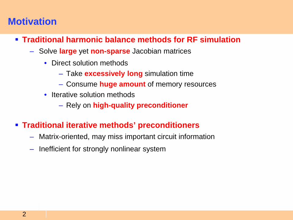
Motivation
Traditional harmonic balance methods for RF simulation– Solve large yet non-sparse Jacobian matrices
• Direct solution methods– Take excessively long simulation time– Consume huge amount of memory resources
• Iterative solution methods– Rely on high-quality preconditioner
Traditional iterative methods’ preconditioners – Matrix-oriented, may miss important circuit information
– Inefficient for strongly nonlinear system
3
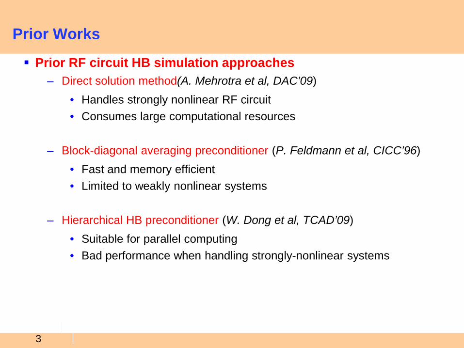
Prior Works
Prior RF circuit HB simulation approaches– Direct solution method(A. Mehrotra et al, DAC’09)
• Handles strongly nonlinear RF circuit• Consumes large computational resources
– Block-diagonal averaging preconditioner (P. Feldmann et al, CICC’96)• Fast and memory efficient• Limited to weakly nonlinear systems
– Hierarchical HB preconditioner (W. Dong et al, TCAD’09)• Suitable for parallel computing• Bad performance when handling strongly-nonlinear systems
4
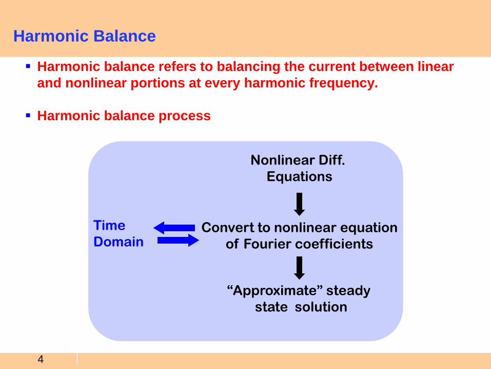
Harmonic Balance
Harmonic balance refers to balancing the current between linear and nonlinear portions at every harmonic frequency.
Harmonic balance process
Nonlinear Diff. Equations
Convert to nonlinear equationof Fourier coefficients
“Approximate” steadystate solution
TimeDomain
5
Harmonic Balance Analysis(1)
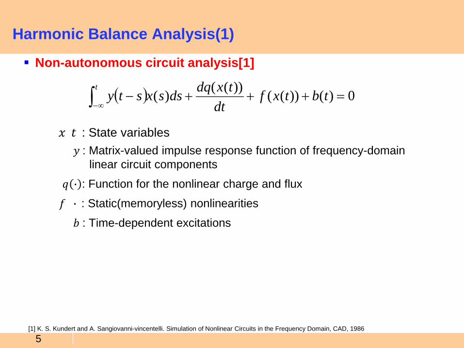
Non-autonomous circuit analysis[1]
𝑥𝑥(𝑡𝑡): State variables𝑦𝑦 : Matrix-valued impulse response function of frequency-domain
linear circuit components
𝑞𝑞 : Function for the nonlinear charge and flux
𝑓𝑓 (): Static(memoryless) nonlinearities
𝑏𝑏 : Time-dependent excitations
[1] K. S. Kundert and A. Sangiovanni-vincentelli. Simulation of Nonlinear Circuits in the Frequency Domain, CAD, 1986
( ) 0)())(())(()( =+++−∫ ∞−tbtxf
dttxdqdssxsty
t
6
Harmonic Balance Analysis(2)
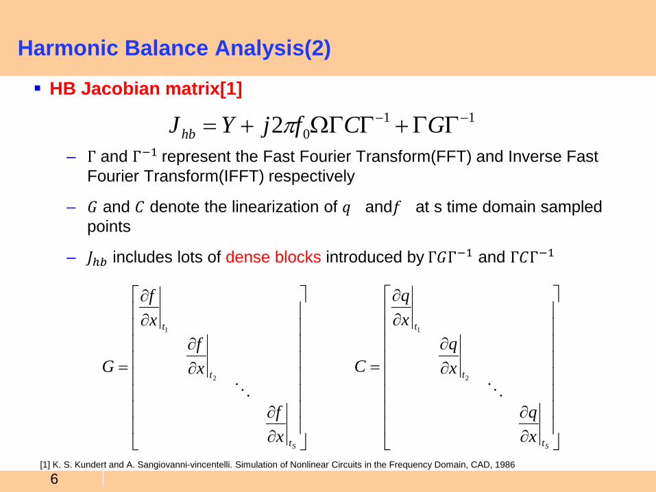
HB Jacobian matrix[1]
– Γ and Γ−1 represent the Fast Fourier Transform(FFT) and Inverse Fast Fourier Transform(IFFT) respectively
– 𝐺𝐺 and 𝐶𝐶 denote the linearization of 𝑞𝑞()and𝑓𝑓()at s time domain sampled points
– 𝐽𝐽ℎ𝑏𝑏 includes lots of dense blocks introduced by Γ𝐺𝐺Γ−1 and Γ𝐶𝐶Γ−1
[1] K. S. Kundert and A. Sangiovanni-vincentelli. Simulation of Nonlinear Circuits in the Frequency Domain, CAD, 1986
1102 −− ΓΓ+ΓΩΓ+= GCfjYJhb π
∂∂
∂∂
∂∂
=
St
t
t
xq
xq
xq
C
2
1
∂∂
∂∂
∂∂
=
St
t
t
xf
xf
xf
G
2
1
7
Our Proposed SCPHB Method
Our proposed method: support-circuit preconditioned HB (SCPHB) iterative solver:
– Effective for solving RF nonlinear circuits
– Scalable linearized RF circuit sparsification
– Circuit-oriented preconditioner generation
– Adaptive support-circuit sparsification
– Matrix-free iterative solver
8
Graph Sparsification Techniques
General linear circuit analysis problems can be converted to equivalent weighted, undirected graph problems
The Laplacian matrix A of a graph – Defined by the quadratic form it induces, which is also known as the
admittance matrix in circuit theory
),,( wEVG =
𝑉𝑉 : a set of vertices𝐸𝐸 : a set of edges𝑤𝑤 : a weight function that assigns a positive weight to every edge
∑∈
−=Eds
dsT dxsxwAxx
),(
2, ))()((
9
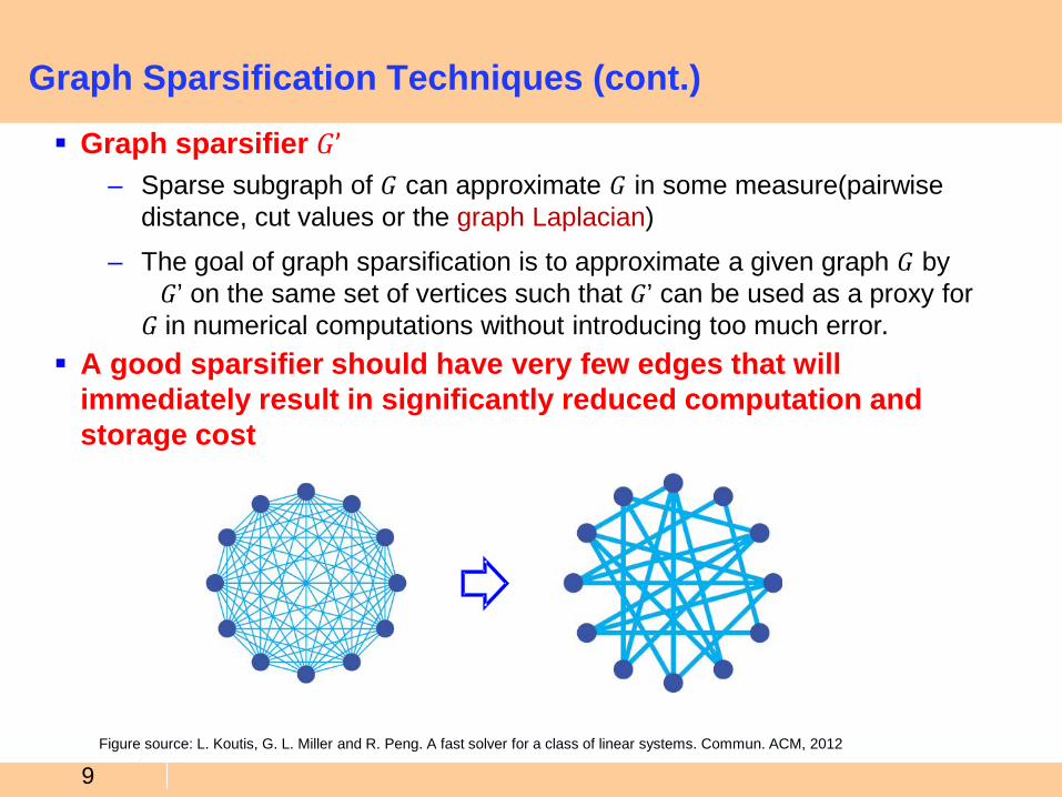
Graph Sparsification Techniques (cont.)
Graph sparsifier 𝐺𝐺𝐺– Sparse subgraph of 𝐺𝐺 can approximate 𝐺𝐺 in some measure(pairwise
distance, cut values or the graph Laplacian)
– The goal of graph sparsification is to approximate a given graph 𝐺𝐺 by𝐺𝐺’ on the same set of vertices such that 𝐺𝐺’ can be used as a proxy for
𝐺𝐺 in numerical computations without introducing too much error. A good sparsifier should have very few edges that will
immediately result in significantly reduced computation and storage cost
Figure source: L. Koutis, G. L. Miller and R. Peng. A fast solver for a class of linear systems. Commun. ACM, 2012
10
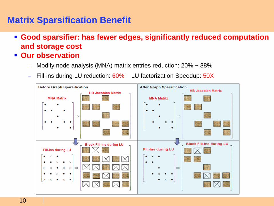
Good sparsifier: has fewer edges, significantly reduced computation and storage cost
Our observation– Modify node analysis (MNA) matrix entries reduction: 20% ~ 38%
– Fill-ins during LU reduction: 60% LU factorization Speedup: 50X
Matrix Sparsification Benefit
11
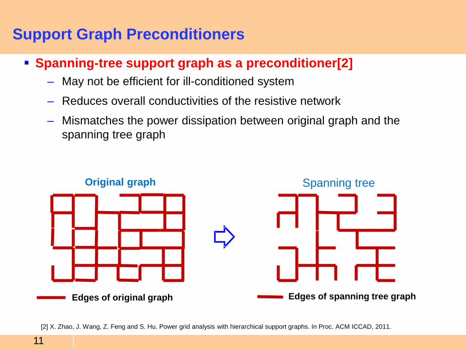
Support Graph Preconditioners
Spanning-tree support graph as a preconditioner[2]– May not be efficient for ill-conditioned system
– Reduces overall conductivities of the resistive network
– Mismatches the power dissipation between original graph and the spanning tree graph
Spanning tree
Edges of spanning tree graph
Original graph
Edges of original graph
[2] X. Zhao, J. Wang, Z. Feng and S. Hu. Power grid analysis with hierarchical support graphs. In Proc. ACM ICCAD, 2011.
12
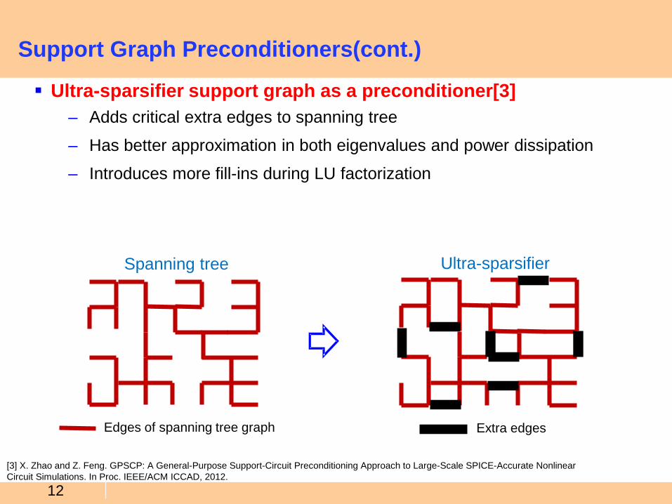
Support Graph Preconditioners(cont.)
Ultra-sparsifier support graph as a preconditioner[3]– Adds critical extra edges to spanning tree
– Has better approximation in both eigenvalues and power dissipation
– Introduces more fill-ins during LU factorization
Spanning tree
Edges of spanning tree graph Extra edges
Ultra-sparsifier
[3] X. Zhao and Z. Feng. GPSCP: A General-Purpose Support-Circuit Preconditioning Approach to Large-Scale SPICE-Accurate NonlinearCircuit Simulations. In Proc. IEEE/ACM ICCAD, 2012.
13
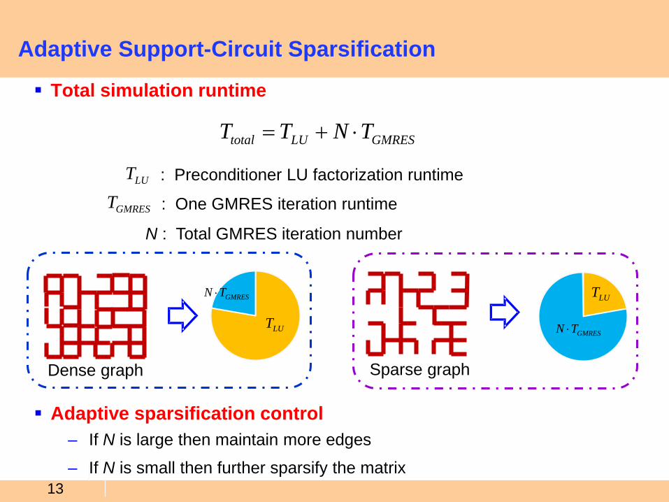
Adaptive Support-Circuit Sparsification
Total simulation runtime
GMRESLUtotal TNTT ⋅+=
N : Total GMRES iteration number
: Preconditioner LU factorization runtimeLUT
: One GMRES iteration runtimeGMREST
Adaptive sparsification control– If N is large then maintain more edges
– If N is small then further sparsify the matrix
LUT
GMRESTN ⋅
Dense graph
LUT
GMRESTN ⋅
Sparse graph
14
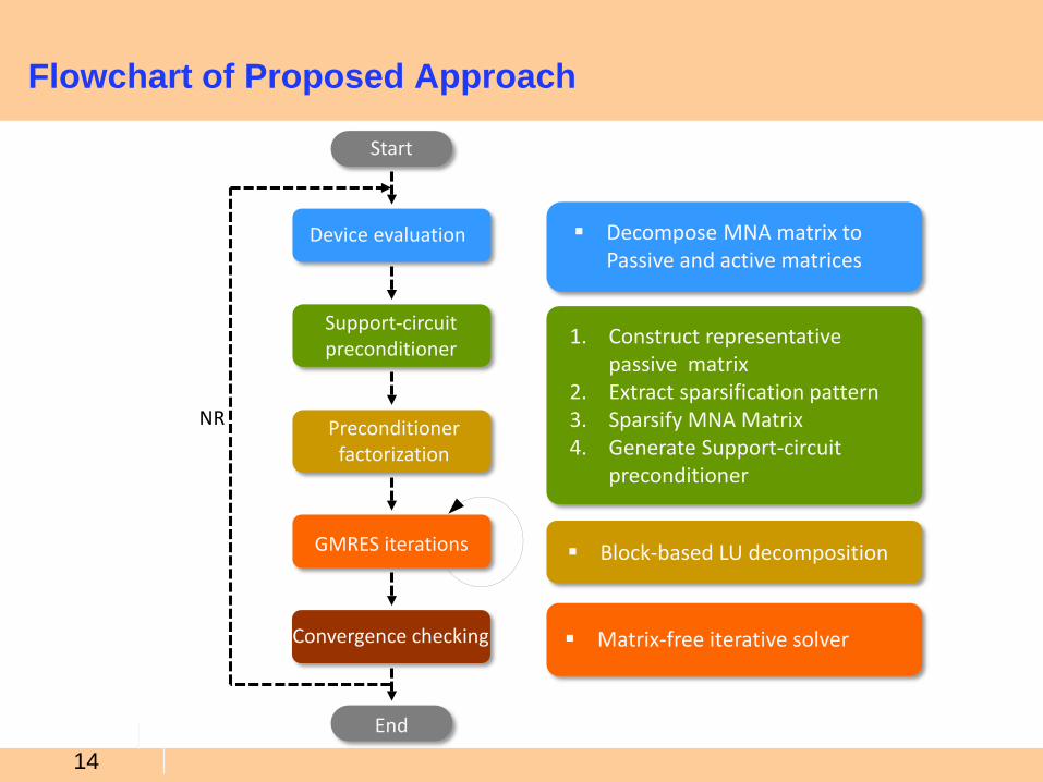
Flowchart of Proposed Approach
Device evaluation
Support-circuitpreconditioner
Preconditionerfactorization
GMRES iterations
Convergence checking
Start
End
NR
Decompose MNA matrix to Passive and active matrices
1. Construct representative passive matrix
2. Extract sparsification pattern3. Sparsify MNA Matrix4. Generate Support-circuit
preconditioner
Block-based LU decomposition
Matrix-free iterative solver
15
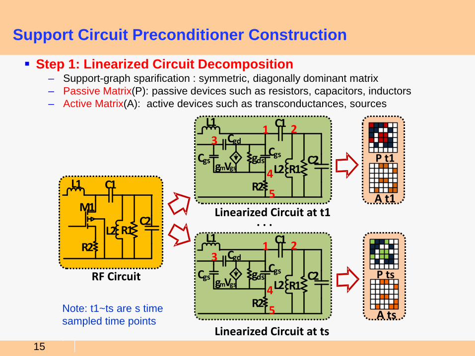
Support Circuit Preconditioner Construction
Step 1: Linearized Circuit Decomposition– Support-graph sparification : symmetric, diagonally dominant matrix – Passive Matrix(P): passive devices such as resistors, capacitors, inductors– Active Matrix(A): active devices such as transconductances, sources
M1
L1
R1L2C2
C1
R2
RF Circuit
Linearized Circuit at t1
Linearized Circuit at ts
. . .
P t1
A t1
L1
R1L2C2
C1Cgd
Cgs gdsCgs
gmVgs
R2
1 23
4
5
L1
R1L2C2
C1Cgd
Cgs gdsCgs
gmVgs
R2
1 23
4
5
P ts
A tsNote: t1~ts are s time sampled time points
16
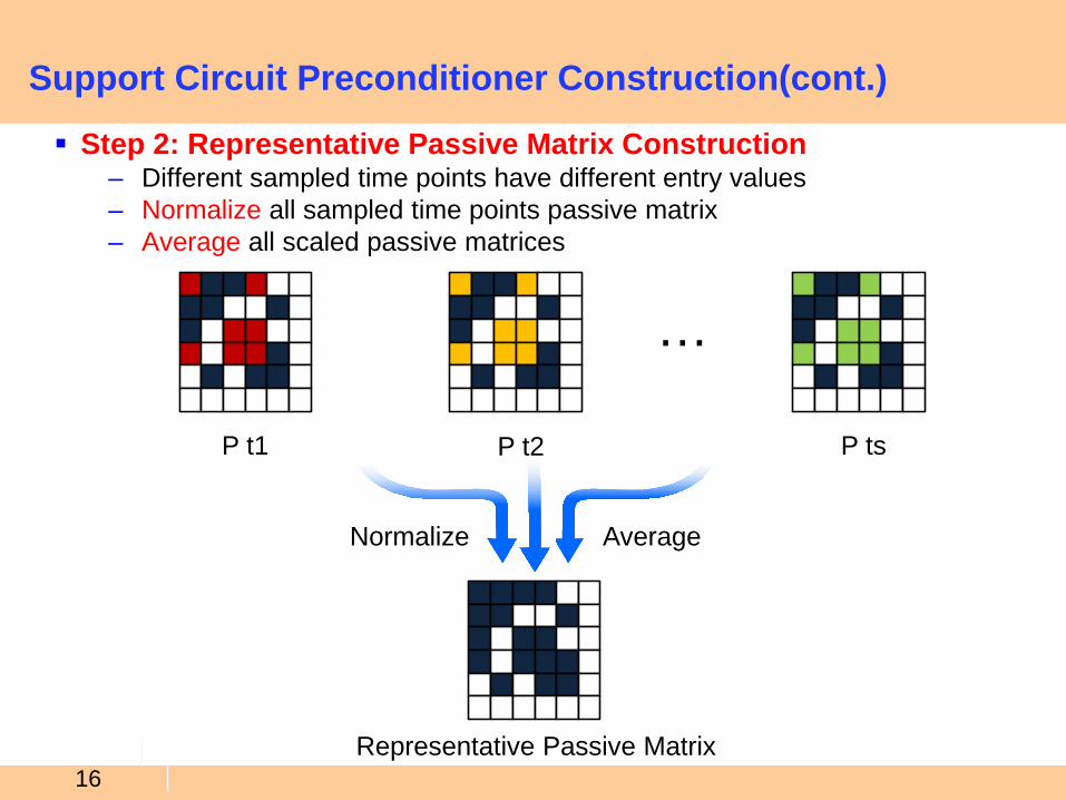
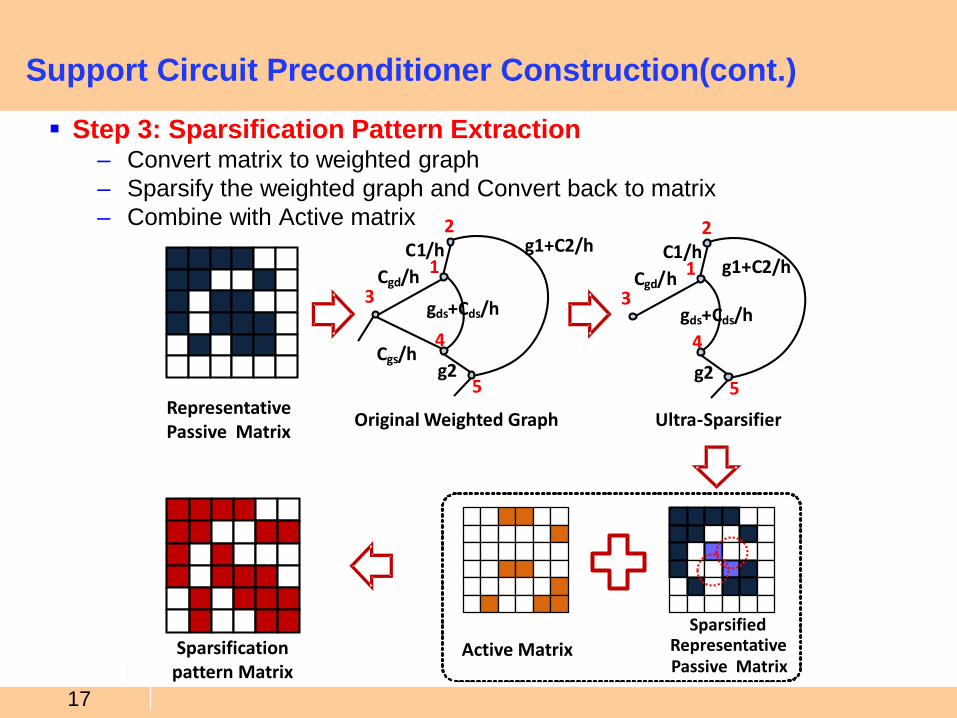
Support Circuit Preconditioner Construction(cont.)
Step 2: Representative Passive Matrix Construction– Different sampled time points have different entry values– Normalize all sampled time points passive matrix – Average all scaled passive matrices
…
P t1 P t2 P ts
Representative Passive Matrix
Normalize Average
17
Support Circuit Preconditioner Construction(cont.)
gds+Cds/h
C1/hCgd/h
31
4g2
Cgs/h
g1+C2/h
5
2
Representative Passive Matrix Original Weighted Graph Ultra-Sparsifier
Sparsified Representative Passive Matrix
Active MatrixSparsification pattern Matrix
C1/hCgd/h
31
4g2
5
2
g1+C2/h
gds+Cds/h
Step 3: Sparsification Pattern Extraction– Convert matrix to weighted graph– Sparsify the weighted graph and Convert back to matrix– Combine with Active matrix
18
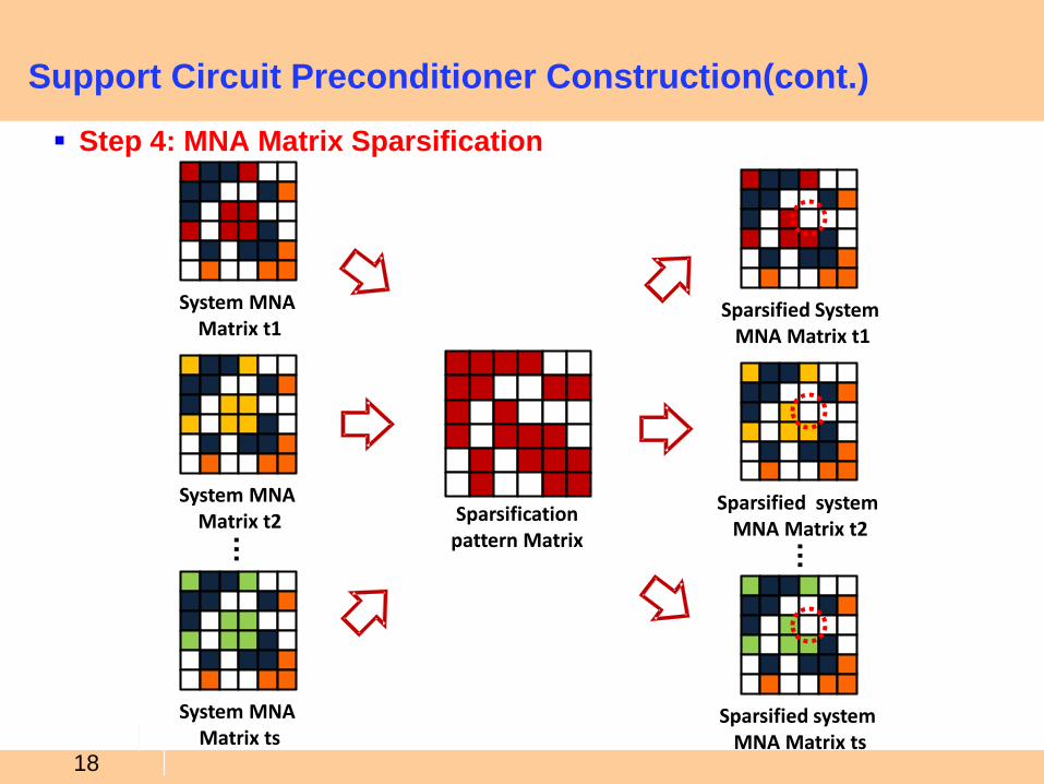
Support Circuit Preconditioner Construction(cont.)
System MNA Matrix t1
Sparsification pattern Matrix
System MNA Matrix t2
System MNA Matrix ts
Sparsified SystemMNA Matrix t1
Sparsified system MNA Matrix t2
Sparsified system MNA Matrix ts
… …
Step 4: MNA Matrix Sparsification
19Support circuit preconditionerPermuted matrix
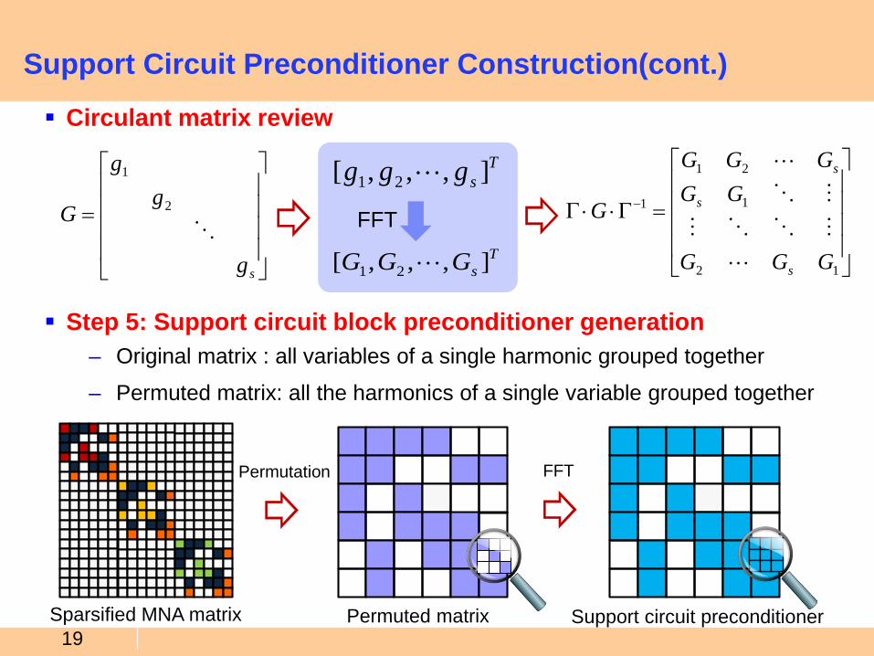
Circulant matrix review
Step 5: Support circuit block preconditioner generation– Original matrix : all variables of a single harmonic grouped together
– Permuted matrix: all the harmonics of a single variable grouped together
Support Circuit Preconditioner Construction(cont.)
=Γ⋅⋅Γ −
12
1
21
1
GGG
GGGGG
G
s
s
s
=
sg
gg
G
2
1
TsGGG ],,,[ 21
Tsggg ],,,[ 21
FFT
Permutation FFT
Sparsified MNA matrix
20
Block Sparse Matrix LU Factorization
Test matrix– Has same sparsity structure as the MNA matrix
– Has representative entries of all sampled time points MNA matrices
– Approximates the properties of block sparse matrix
– Has same permutation and pivoting pattern with block sparse matrix LU factorization
Block sparse matrix LU factorization– Applies permutation and pivoting pattern to block sparse matrix
– Performs LU factorization w/o pivoting
– Uses LAPACK/BLAS for matrix dense block multiplication and division
Matrix-free iterative solver– Implicit system Jacobian matrix
– Explicit preconditioner matrix which has limited entries
21
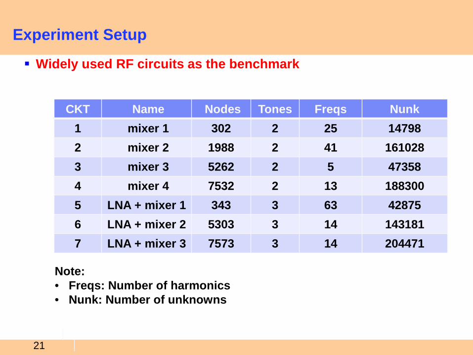
Experiment Setup
Note:• Freqs: Number of harmonics• Nunk: Number of unknowns
CKT Name Nodes Tones Freqs Nunk1 mixer 1 302 2 25 147982 mixer 2 1988 2 41 1610283 mixer 3 5262 2 5 473584 mixer 4 7532 2 13 1883005 LNA + mixer 1 343 3 63 428756 LNA + mixer 2 5303 3 14 1431817 LNA + mixer 3 7573 3 14 204471
Widely used RF circuits as the benchmark
22
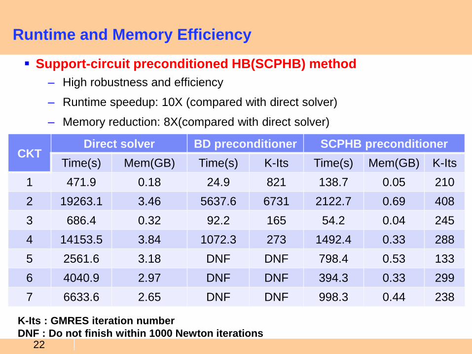
Runtime and Memory Efficiency
CKTDirect solver BD preconditioner SCPHB preconditioner
Time(s) Mem(GB) Time(s) K-Its Time(s) Mem(GB) K-Its1 471.9 0.18 24.9 821 138.7 0.05 2102 19263.1 3.46 5637.6 6731 2122.7 0.69 4083 686.4 0.32 92.2 165 54.2 0.04 2454 14153.5 3.84 1072.3 273 1492.4 0.33 2885 2561.6 3.18 DNF DNF 798.4 0.53 1336 4040.9 2.97 DNF DNF 394.3 0.33 2997 6633.6 2.65 DNF DNF 998.3 0.44 238
Support-circuit preconditioned HB(SCPHB) method– High robustness and efficiency
– Runtime speedup: 10X (compared with direct solver)
– Memory reduction: 8X(compared with direct solver)
K-Its : GMRES iteration numberDNF : Do not finish within 1000 Newton iterations
23
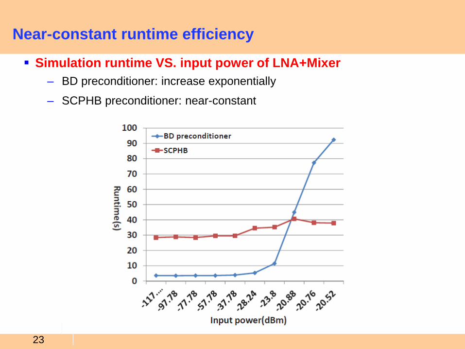
Near-constant runtime efficiency
Simulation runtime VS. input power of LNA+Mixer– BD preconditioner: increase exponentially
– SCPHB preconditioner: near-constant
24
Conclusion
A scalable Jacobian matrix solving method is proposed for tackling frequency-domain strongly nonlinear HB analysis
Our experimental results show that SCPHB method can attain:– Obtain up to 10X speedups in RF HB simulations
– Reduce up to 8X memory consumption
Key ideas :– Use ultra-sparsifier support circuit as the preconditioner
– Use block sparse LU matrix solver for factorizing the preconditioner
– Use matrix-free iterative solver
– Use adaptive sparsification control to get best overall runtime
Recommended


![Graph Partitioning for Scalable Distributed Graph Computations04]-BulucMadduri_DIMACS_w… · Scalable Distributed Graph Computations Ayd n Bulu˘c1 and Kamesh Madduri2 1 Lawrence](https://img.pdfslide.us/doc/110x75/5f19c29095667b31881113f2/graph-partitioning-for-scalable-distributed-graph-04-bulucmadduridimacsw-scalable.jpg)


![Spectral Algorithms for Temporal Graph Cutsarlei/pubs/ · theory [9], a subject with great impact in information retrieval [29], graph sparsification [46], and machine learning [27]](https://img.pdfslide.us/doc/110x75/5f29457f34eee82c013bbc29/spectral-algorithms-for-temporal-graph-cuts-arleipubs-theory-9-a-subject.jpg)