American Journal of Theoretical and Applied Statistics 2015; 4(6): 446-463
Published online October 10, 2015 (http://www.sciencepublishinggroup.com/j/ajtas)
doi: 10.11648/j.ajtas.20150406.15
ISSN: 2326-8999 (Print); ISSN: 2326-9006 (Online)
An Assessment of Farmers Livelihood in the Coffee Certification Schemes in Tanzania
Charles Kipkorir Masson
Department of Statistics and Computer Science, Moi University, Eldoret, Kenya
Email address:
To cite this article: Charles Kipkorir Masson. An Assessment of Farmers Livelihood in the Coffee Certification Schemes in Tanzania. American Journal of
Theoretical and Applied Statistics. Vol. 4, No. 6, 2015, pp. 446-463. doi: 10.11648/j.ajtas.20150406.15
Abstract: This study was undertaken to assess the impacts of adoption of various types of coffee certifications on the
livelihoods of smallholder farmers. The main objective of this study was to compare the livelihood of farmers under the
different producer groups with respect to their income and food security situation. It begins with an introduction to impact
assessment and a description of the methodology and its challenges with an outline of the method used for handling outliers
and comparing the certified and non-certified farmers and the producer groups. Secondary data from coffee survey data
collected by COSA and partners for analyzing the impact of sustainability standards forms the basis of this study. Multi stage
cluster sampling was used to sample farmers that were interviewed. In the first stage, the coffee growing areas in Tanzania and
the active certification programs were identified. Then second level producer groups that had obtained certification were used
to obtained the sampling frame of the first level producer groups. Random sampling was then used to select the first level
producer groups and also randomly select villages with farmer in the producer groups. Non parametric methods have been used
to compare the producer groups because one sample does not follow a normal distribution and most of them are highly skewed.
Error bars plots have been used to compare the significance difference in the producer groups. Aggregate income from the
different forms in which coffee was sold has been computed and used for comparison. It also evaluates the food security
situation last production year of the farmers across the different producer groups. The key indicators used, showed that
generally, adoption of the various coffee certifications programs have positive impacts on income and food security. In the
course of this study, the areas of further research that emerged are; an evaluation of the farmers livelihood before intervention
is done to ascertain whether their livelihood has changed due to adoption of certification or due to other factors and the
development of a stepwise procedure for an outlier identification and ascertaining their validity. The methods that were used
for outlier detection were subjective.
Keywords: Coffee Certifications, Smallholder Farmers, Livelihoods Assessment, Outlier Detection
1. Introduction
1.1. Impact Assessment
Carney (1998) defined livelihood to comprise the capabilities,
assets (including both material and social resources) and
activities required for a means of living. A livelihood is
sustainable when it can cope with and recover from stresses and
shocks and maintain or enhance its capabilities and assets both
now and in the future, while not undermining the natural
resource base. Impact Assessment is a process of systematic and
objective identification of the short and long-term effects which
can be positive or negative, direct or indirect, intended or
unintended, primary and secondary on households, institutions
and the environment caused by on-going or completed
development activities such as a programs or projects. The term
impact is the difference between what would happen with the
action and what would happen without it. The purpose of impact
assessment is to help in a better understanding of the extent of
activities, objectives fulfilled and magnitude of effects. IA
involves observing, measuring and describing how the
conditions being assessed have been influenced. Impact is given
by direct effects on income from increased adoption and use of
technologies. This can be measured by the number of farmers or
area planted with an improved technology, yield increase
productivity growth and economic effects of adoption of new
technologies. The indicators by which a program is to be
assessed are taken to be given, as appropriate to the type of
program. Knowing impact is of obvious interest in its own right
as a means of measuring the aggregate benefits from the

447 Charles Kipkorir Masson: An Assessment of Farmers Livelihood in the Coffee Certification Schemes in Tanzania
program. However, when reducing poverty is the overall
objective of the program we also want to know the incidence of
the welfare gains (Ravallion, 2003)
IAs assess the difference in the values of key variables
between the outcomes on 'agents' (individuals, enterprises,
households, populations, policymakers etc) which have
experienced an intervention against the values of those
variables that would have occurred had there been no
intervention (Hulme, 1997) IA studies have recently become
popular with donor agencies and, in consequence, have
become an increasingly significant activity for recipient
agencies. In part this reflects a cosmetic change, with the term
IA simply being substituted for evaluation. But it has also been
associated with a greater focus on the outcomes of
interventions, rather than inputs and outputs. While the goals
of IA studies commonly incorporate both 'proving' impacts and
'improving' interventions, IAs are more likely to prioritize the
proving goal than did the evaluations of the 1980s. A set of
factors are associated with the extreme 'pole' positions of this
continuum and these underpin many of the issues that must be
resolved (and personal and institutional tensions that arise)
when impact assessments are being initiated (Hulme, 1997)
1.2. Methodological Challenges
In surveys, the quality of data means that considerable
efforts have been made to calculate metadata about quality to
support the series being produced. Metadata for this purpose
come in a variety of styles; in some cases they are readily
calculated through theory, such as sampling errors. In other
cases the quality aspect which is of primary interest is not
easily measured, such as non-response bias, but a relatively
easy calculation- the response rate - gives an indicator for the
magnitude of either the bias, or perhaps the risk that the bias
will be large enough to affect the interpretation of the
statistics. In a few cases, such as measurement error, there is
very little that can be done with survey data and the only real
way to measure the quality is to do an expensive follow-up
study. In other dimensions there is no direct quantification
(for example, relevance), and then only circumstantial
information can be provided. In this study data was
downloaded into a single spreadsheet instead of multiple
sheets for ease in navigation. Metadata given partially
qualities the data they describe and a number of variables are
categorical which limit the type of analysis to be done.
1.3. Statement of the Problem
Coffee production is the main livelihood strategy for most of
the smallholder farmers and the use of coffee certification has
been the principal means of maintaining the sustainability of
farmers' livelihoods. They have been growing coffee for a long
period with the expectation that their livelihood would
improve significantly but ironically it has constantly stagnated
and in worst circumstances continued to deteriorate despite the
adoption of new technologies of coffee production. To avert
these trends it is necessary to evaluate the revenue earned from
engaging in coffee production. The farmers' yields have been
based on subjective estimates which are not accurate in
calculation of revenue accrued from farming.
1.4. Objectives
The main objective of the study was to compare the
livelihood of farmers under the different producer groups
with respect to their income and food security situation. The
study was guided by the following specific objectives
i. To explore data and identify the outliers
ii. To compare the different producer groups income.
iii. To compare the different producer groups food security
situation.
iv. To find the relationship between income and food
security situation.
2. Litrature Review
2.1. Coffee Certifications
Declining coffee prices considerably affect the livelihoods
of producer farmers as they largely depend on income from
coffee to meet most of their basic household needs. Lower
prices mean, for instance, that they cannot afford to send
their children to school, buy medicines or food. According to
(Mayne et al., 2002), many farmers were forced to sell assets
such as cattle and cut essential expenses, including food,
during the price slump between 1999 and 2002. Smallholder
livelihoods suffered when international coffee commodity
prices plummeted from 1999_2004. In response to the coffee
crisis, non-governmental organizations (NGOs), selected
coffee companies, and several coffee producer cooperatives
spearheaded efforts to expand sustainable coffee certification
programs (Bacon et al., 2008).The impacts of the drop in
coffee prices on small-scale and micro producers (fewer than
14 hectares) included rapidly declining incomes, resulting in
hunger, crop abandonment, and a series of issues that we
explore more deeply in the following sections. The owners of
medium-scale farms (14 to 35 hectares) often stopped
employing farm workers and decreased management
intensity. The largest plantations (more than 35 hectares)
employed most of the farm workers and had higher monetary
costs of production due to dense cropping patterns,
dependence on paid labor, and intensive chemical inputs.
When international coffee prices were high, high yields and
low wages contributed to a profitable operation. When the
prices fell below the costs of production, banks stopped
offering credit and foreclosed on debt-ridden large
landholdings (Bacon et al., 2008).
Certification is an instrument to add value to a product,
and it addresses a growing worldwide demand for healthier
and more socially and environmentally-friendly products. It
is based on the idea that consumers are motivated to pay
price pre-mia for products that meet certain precisely defined
and assured standards (Ponte, 2004b). The social and
economic challenges small-scale coffee producers face today
in many coffee producing countries has given strong impetus
to the Fair trade movement. Fair trade is a voluntary
American Journal of Theoretical and Applied Statistics 2015; 4(6): 446-463 448
certification scheme that seeks to challenge the unequal terms
of trade in the global coffee value chain to facilitate
sustainable development. Fair trade is an alternative trade
initiative promoting a different approach both to the
conventional global trading system (free trade) and to
development systems (protectionism and development aid)
through the philosophy of 'trade-not-aid' (Raynolds, 2002)
Certifications are often seen as a solution to problems to the
instable commodity markets. Certification schemes have
emerged as one approach to try and raise the economic,
social and environmental standards of coffee production and
as well as trade (Ponte, 2004a).
2.2. Livelihood Assessment
A livelihood comprises the capabilities, assets and
activities required for a means of living. The assets include
natural, material and social resources such land, livestock,
machines, tools, stocks of money, education, skills and social
networks while activities Include productive ventures such as
farming and livestock keeping. Current understanding of
livelihoods place considerable emphasis on the ownership or
access to assets that can be put to productive use as the
building blocks by which the poor can make their living
(Ellis, 2000). Bania et al. (2007) observed that many simple
correlations have been noted between food insufficiency and
a range of factors, including the level of household income,
food stamp receipt, demographics, household composition,
education, physical and mental health status, and geography.
Lewis (2005) analyzed the Mexican coffee sector focusing on
the links among low coffee prices, migration, and certified
coffee production and trade. The results show that although
remittances from migrants help finance coffee production,
increased migration drains human capital out of the region
which again raises the opportunity cost of labor and hence
local wages, thus raising the costs of coffee production.
The findings raise doubts about the sustainability of the
Fair Trade-organic coffee model in the face of migration
opportunities. According to Bacon (2005), in the Nicaraguan
context that Fair trade and organic networks can provide
security and increased income, but do not offset the many
factors leading to a general decline in quality of life for the
farmers. Wollni and Zeller (2007) used data from coffee
farmers in Costa Rica and determine the factors which make
farmers participate in a specialty coffee market. They find
that significant price pre-mia are received by certified
farmers as opposed to their noncertified counterparts and that
social capital, if captured in terms of participating in a
cooperative, is highly significant for the decision to grow
specialty coffee. The findings of Dasgupta (1989), revealed
that the level of education is strong and a significant
determinant of farmers' adoption of improved agricultural
technologies.
2.3. Outlier Detection
The purpose of outlier detection is to discover the unusual
data, whose behavior is very exceptional when compared to
the rest of the data set. Examining the extraordinary behavior
of outliers helps to uncover the valuable knowledge hidden
behind them and to help the decision makers to make profit
or improve the service quality. Hence, mining aiming to
detect outlier is an important data mining research with
numerous applications, which include credit card fraud
detection, discovery of criminal activities in electronic
commerce, weather prediction, marketing, statistical
applications and so on. Detection methods are divided into
two parts: univariate and multivariate methods. In univariate
methods, observations are examined individually and in
multivariate methods, associations between variables in the
same dataset are taken into account. Classical outlier
detection methods are powerful when the data contain only
one outlier. However, these methods decrease drastically if
more than one outliers, are present in the data (Hadi, 1992).
Although outliers are typically detected by comparison
with other observations in a redundant data set, an outlier is
not just an observation that deviates from other observations.
Random errors can be large and, as long as the understanding
of the sources of errors is correct, the Standard Uncertainty
(SU) will be large, and comparable to the size of deviations.
If such an observation is merged with other observations, it
will have an appropriate influence on the mean value,
depending on the precision of other observations. Problems
only arise when the error is much larger than one would
expect from the SU. Therefore, an outlier is an observation
that is unlikely to be correct within error limits(Read, 1999).
3. Methodology
3.1. Source of Data
Secondary data from coffee survey data collected by
COSA and partners for analyzing the impact of sustainability
standards forms the basis of this study. This data was entered
onto an online database and was accessed by downloading
from http://surveys.tcosa.org/CosaSurveys.html in June 2011.
After the launch of the COSA application users can work
with it either on-line or off-line provided that Google gears
are installed. The features of the survey builder enable the
standardized customization so that basic survey can easily be
adapted from different languages, crops and specific
conditions in different countries. The COSA methodology
was built upon a process of annual field visits to farms
located throughout the major growing regions to gather
information based on a common set of measures/indicators.
The basic parameters of the full methodology include;
i. Farm visits over a minimum of a three-year period to
discern measurable changes over time resulting from
the implementation of different initiatives;
ii. Indicator selection criteria using SMART concepts;
iii. Farm selection criteria ensuring balanced representation
across:
� The six major sustainability initiatives operative in the
coffee sector (Organic, Fair
� Trade, 4Cs, Utz Certified, Rainforest Alliance and
449 Charles Kipkorir Masson: An Assessment of Farmers Livelihood in the Coffee Certification Schemes in Tanzania
Starbucks C.A.F.E. Practices);
� Major coffee growing regions (Africa, Asia and Latin
America)
� Small and large farms (based on national norms); -
Distinct agro-ecological zones (rainfall, altitude, etc.);
� Coffee types (Robusta, Arabica, etc.); and
� Different production systems (traditional shade,
intensive sun, etc.).
COSA envisions the future global availability of
comparably-defined data so that producers and policy-makers
can better determine how they compare with producers
operating in different regions or applying similar or different
standards (Giovannucci et al., 2008).
A sample of 1035 farmers was interviewed and
information collected included the socio-economic
characteristics of farmers, inputs and outputs of coffee,
assets, factors of production such as labor and fertilizers
that were used as well as their costs. Socioeconomic
variables such as the level of education, number of years of
coffee farming, land tenure situation and use of improved
coffee varieties.
3.2. Sampling
The geographical areas in the North, South and West of
Tanzania that from which sampling was done covers 80% of
the coffee growers. Multi stage cluster sampling was used to
sample farmers that were interviewed. In the first stage, the
coffee growing areas in Tanzania and the active certification
programs were identified. Then second level producer groups
that had obtained certification were used to obtained the
sampling frame of the first level producer groups. Random
sampling was then used to select the first level producer
groups and also randomly select villages with farmer in the
PG. From the sampling frame of first level PG members,
farmers were randomly selected from the selected villages.
After selection of the second level PGs with the certification,
the certified treatment groups were identified, these were:
Starbucks C.A.F.E Practices (CP), Fare Trade (FT), Organic,
FT and Utz, FT and Organic and FT and CP, PGs operating
with similar conditions to the certified groups were identified
and approached them on obtaining the lists to sample their
members. Farmers were then selected from these second
level groups by a process similar to that for the certified
sample. In this study, the term 'producer' has been to mean
the person(s) responsible for the production of the
commodity on the farm. In most cases the smallholders (who
can be of female or male gender) will be the farm owners
themselves, but it may also be a farm manager, caretaker or
the person who can provide information regarding farm
management and production.
3.3. Variable Selection
The key indicators (Table 1) that were used in this study
were identified, retrieved and aggregated to generate the
indicators.
Table 1. Key Indicators.
Key indicators Type
Certification Categorical
sr__group_name_cat Categorical
Block_income_revenue_all_target_crop_revenue Continuous
Total_crop_revenue Continuous
Coffee_revenue_per_ha Continuous
Revenue_ha Continuous
Price_cert_sold_uncert Continuous
Price_uncert Continuous
Average_price_all_coffee_sold Continuous
Zero_days_hunger Categorical
One_nine_days_hunger Categorical
Ten_twentynine_days_hunger Categorical
Thirty_or_more_days_hunger Categorical
The income indicator variables (Table 1) were computed
by aggregating the variables on the second column, all the
food security variables that were used are categorical.
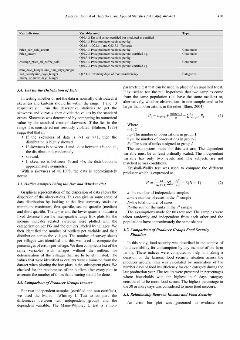
Table 2. Variables that were used to generate the key indicators.
Key indicators Variables used Type
Block_income_revenue
Q10.3.3-Kg coffee sold
Q10.3.4-Price producer received per kg
Q10.4.2-Kg sold as not certified but produced as certified
Q10.4.3-Price producer received per kg
Continuous
Total_crop_revenue
Q10.2.2-Kg of not certified coffee sold
Q10.2.3-Price producer received per not certified kg
Q10.3.3-Kg coffee sold
Q10.3.4-Price producer received per kg
Q10.4.2-Kg sold as not certified but produced as certified
Q10.4.3-Price producer received per kg
Q23.1-How much was the income.
Continuous
Coffee_revenue_per_ha
Q10.2-Kg of not certified coffee sold
Q10.2.3-Price producer received per not certi_ed kg
Q10.3.3-Kg coffee sold
Q10.3.4-Price producer received per kg
Q10.4.2-Kg sold as not certified but produced as certified
Q10.4.3-Price producer received per kg
Q22.5.1, Q22.6.1 and Q22.7.1- Plot area.
Continuous
Revenue_ha Q10.3.3-Kg coffee sold
Q10.3.4-Price producer received per kg Continuous
American Journal of Theoretical and Applied Statistics 2015; 4(6): 446-463 450
Key indicators Variables used Type
Q10.4.2-Kg sold as not certified but produced as certified
Q10.4.3-Price producer received per kg
Q22.5.1, Q22.6.1 and Q22.7.1- Plot area.
Price_cert_sold_uncert Q10.4.3-Price producer received per kg Continuous
Price_uncert Q10.2.3-Price producer received per not certified kg. Continuous
Average_price_all_coffee_sold
Q10.3.4-Price producer received per kg
Q10.4.3-Price producer received per kg
Q10.2.3-Price producer received per not certified kg.
Continuous
zero_days_hunger One_nine_days_hunger
Ten_twentynine_days_hunger
Thirty_or_more_days_hunger
Q17.1- How many days of food insufficiency Categorical
3.4. Test for the Distribution of Data
In testing whether or not the data is normally distributed, it
skewness and kurtosis should lie within the range ±1 and ±3
respectively. I run the descriptive statistics to get the
skewness and kurotsis, then divide the values by the standard
errors. Skewness was determined by comparing its numerical
value by the standard error of skewness. If the lies in the
range it is considered not seriously violated. (Bulmer, 1979)
suggested that if;
� If the skewness of data is <-1 or >+1, then the
distribution is highly skewed
� If skewness is between -1 and -½ or between +½ and +1,
the distribution is moderately
� skewed.
� If skewness is between -½ and +½, the distribution is
approximately symmetric.
With a skewness of =0.1098, the data is approximately
normal.
3.5. Outlier Analysis Using the Box and Whisker Plot
Graphical representation of the dispersion of data shows the
dispersion of the observations. This can give us some sense of
data distribution by looking at the five summary statistics:
minimum, maximum, first quartile, second quartile (median)
and third quartile. The upper and the lower quartile indicate a
fixed distance from the inter-quartile range Box plots for the
income indicator related variables were plotted with the
categorization per PG and the outliers labeled by villages. We
then identified the number of outliers per variable and their
distribution across the villages. The number of survey sheets
per villages was identified and this was used to compute the
percentages of errors per village. We then compiled a list of the
same variables with villages without the outliers for
determination of the villages that are to be eliminated. The
values that were identified as outliers were eliminated from the
dataset when plotting the box plots in the subsequent plots. We
checked for the randomness of the outliers after every plot to
ascertain the number of times that cleaning should be done.
3.6. Comparison of Producer Groups Income
For two independent samples (certified and non-certified),
we used the Mann - Whitney U Test to compare the
differences between two independent groups and the
dependent variable. The Mann-Whitney U test is a non-
parametric test that can be used in place of an unpaired t-test.
It is used to test the null hypothesis that two samples come
from the same population (i.e. have the same median) or,
alternatively, whether observations in one sample tend to be
larger than observations in the other (Shier, 2004)
�� = ���� + �(���)� −∑ ����
������ (1)
Where
i=1, 2
��=The number of observations in group 1
��=The number of observations in group 2
Ri=The sum of ranks assigned to group i
The assumptions made for this test are; The dependent
variable must be as least ordinally scaled, The independent
variable has only two levels and The subjects are not
matched across conditions.
Kruskall-Wallis test was used to compare the different
producer which is expressed as;
� = � ���(���)∑
���
���� � − 3(� + 1) (2)
k=the number of independent samples
ni=the number of cases in the ith
sample
N=the total number of cases
Ri=the sum of the ranks in the ith
sample
The assumptions made for this test are: The samples were
taken randomly and independent from each other and the
populations have approximately the same shapes
3.7. Comparison of Producer Groups Food Security
Situation
In this study, food security was described in the context of
food availability for consumption by any member of the farm
family. These indices were computed to help in making a
decision on the farmers' food security situation across the
producer groups. This was calculated by summation of the
number days of food insufficiency for each category during the
last production year. The results were presented in percentages
where households with the highest in 0 days category
considered to be more food secure. The highest percentage in
the 30 or more days was considered to more food insecure.
3.8. Relationship Between Income and Food Security
An error bar plot was generated to evaluate the

451 Charles Kipkorir Masson: An Assessment of Farmers Livelihood in the Coffee Certification Schemes in Tanzania
relationship between the farmers income and food security
situation. Block income revenue was plotted against the four
categories (0 days 1-9 days, 10-29 and 30+ days).
4. Empirial Results and Discussion
4.1. Test for Normality
In this study, research tested for the normality of the
dataset by running descriptive statistics to get the skewness
and kurtosis together with their respective standard errors. It
was found out that the SE of skewness for FT South was
beyond the expected interval (-0.366 and +0.366). In a
normal distribution the values of skewness and kurtosis are
zero. The positive values indicate a pile of data points on the
left of the distribution whereas the values indicate a pile up
of data points to the right of the distribution. The further
these values are from zero the more unlikely it is that data are
not normally distributed. Histogram and Q-Q plot for the
block income revenue all target crop was plotted as a
representative for the other indicators.
Figure 1. Residual plots for the block income.
The graphical representation (Figure 1) displays that this
data does not assume normality. The histogram shows
asymmetrical bell-shape with a normal curved superimposed
with more of the values lying to the left in the left than those
to the right. The Q-Q plot has a line almost 45 degrees to the
origin but the observations appear to deviate more from the
fitted line. These results and those from the descriptive
analysis suggests that all the samples do not follow a normal
distribution hence used non Parametric methods for
comparison of the certification types and PGs.
Table 3. Distribution of the producer groups per certification types.
Percentage
Producer groups Certified Non-Certified
A.F.E. Practices Control Mbozi 0 18.0
C.A.F.E. Practices Lima 147.7 0
Fair trade South 20.0 0
Fair trade North 10.0 0
Fair trade North/Fair Trade and Organic
Control 0 21.8
Fair trade South/Fair trade and Utz Control 0 27.3
Fair trade and C.A.F.E. Practices Control 0 12.8
Fair trade and C.A.F.E. Practices Kilicafe 17.3 0
Fair trade and Organic 16.7 0
Fair trade and Utz 19.2 0
Organic 20.0 0
Organic Control 0 20.0
4.2. The Distribution of the Producer Groups
This survey consisted of 12 producer groups which were
classified as either certified or non-certified, the farmers who
were sampled were distributed (Table 3). These were
sampled from 122 villages and 52.7% of the farmers were
certified while 47.3% were non certified. In the certified
group of farmers, FT and Utz had the highest percentage
(19.2%) and among the non-certified group FT south/FT and
Utz control had the highest percentage (27.3%).
4.3. Outliers’ Analysis Using Box and Whisker Plots
4.3.1. Sequential Identification of Outliers
Further exploratory analysis of the variables was done
using box plots to display the spread of the data a glance.
This presented the overall shape of the graphed data which
included its symmetry and departure from assumptions.
According to Hawkins (1980) an outlier defined as an
observation that deviates so much from other observations as
to arouse suspicion that it was generated by a different
mechanism.(Johnson and Wichern, 2002) also defined an
outlier as an observation in a dataset which appears to be
inconsistent with the remainder of that set of data. In this
study, we have considered the outliers as the data that lie

American Journal of Theoretical and Applied Statistics 2015; 4(6): 446-463 452
outside the expected range of data distribution and it
necessary to conduct an outlier analysis for the purpose of
data validation. This can indicate errors and since the data
used in this study is secondary data, it was not possible to
check whether these outliers were indeed true values or
erroneous data. Erroneous data can be caused by either; the
enumerators during data collection (non-random) and data
entry (random).
Davies and Gather (1993) came up with an important
distinction between single-step and sequential procedures for
outlier detection. Single step procedures identify all outliers
at once as opposed to successive elimination or addition of
datum. In the sequential procedures, at each step, one
observation is tested for being an outlier. Outliers caused by
errors may occur frequently, while outliers caused by events
tend to have extremely smaller probability of occurrence
(Martincic and Schwiebert, 2006)
Erroneous data is normally represented as an arbitrary
change and is extremely different from the rest of the data.
Due to the fact that such errors influence data quality, they
need to be identified and corrected if possible as data after
correction may still be usable for data analysis. Before we
address the issue of identifying these outliers, we must
emphasize that not all are wrong numbers. They may
justifiably be part of the group and may lead to better
understanding of the phenomena being studied. When an
outlier is detected, the analyst is faced with number of
questions (Andrews and Pregibon, 1978);
� Is the measurement process out of control?
� Is the model wrong?
� Is some transformation required?
� Is there an identifiable subset of observations that is
important in its different behavior?
An exploratory analysis on the income indicators was done
using box and whisker plots to display the spread of the data
at a glance. This presented the overall shape of the graphed
data which included its symmetry and departure from
assumptions. In this study, total crop revenue was used as
example for all the 7 indicators.
Figure 2. Distribution of outliers in original data.
From Figure 2, all the PGs had outliers, C.A.F.E practices
control Mbozi showed the highest variability of the
observations and the highest number (12) of outliers all
above the upper whisker, C.A.F.E practices Lima showed 4
outliers above the upper whisker, FT south, FT north and FT
north/FT and organic control and Fair trade South/Fair trade
and Utz Control showed less variability with each showing
two outliers. Fair trade and C.A.F.E. Practices Control and
Fair trade and C.A.F.E. Practices Kilicafe and Fair trade and
Organic showed outliers clustered around the upper whisker.
Fair trade and Utz had 4 values as outliers. Organic and
Organic Control also had the outliers clustered around the
two whiskers. There was minimal variability in the
observations in most of the producer groups. The outliers
were randomly distributed and all the PGs had at least one
outlier.
In Figure 3, all the box plots except for Fair trade South
were clear when the outliers were deleted in the original
dataset and their number are reduced. C.A.F.E practices
control Mbozi still showed extreme values (around 4,000,000)
as outliers. C.A.F.E Practices Lima, Fair trade and C.A.F.E.
Practices Control and Fair trade and C.A.F.E. Practices
Kilicafe all had the same median value each with at least 1
outlier. Fair trade North, Fair trade and Organic, Fair trade

453 Charles Kipkorir Masson: An Assessment of Farmers Livelihood in the Coffee Certification Schemes in Tanzania
and Utz, Organic and Organic Control each had 2 outliers.
Fair trade North/Fair Trade and Organic Control had the
highest number of outliers (7) clustered around the upper
whisker. Fair trade South did not show any outliers. When
high values were eliminated in Figure 1, the outliers were
still random and some of the PGs started showing some
variability.
Figure 3. Distribution of outliers after cleaning data once.
Figure 4. Distribution outliers after cleaning data twice.
In Figure 4, all the PGs showed that at least one existed
with C.A.F.E. Practices Control Mbozi and Fair trade and
C.A.F.E. Practices Control showing extreme values. C.A.F.E
Practices Lima had 1 outlier, Fair trade and C.A.F.E.

American Journal of Theoretical and Applied Statistics 2015; 4(6): 446-463 454
Practices Control and Fair trade and C.A.F.E. Practices
Kilicafe had the same median with 5 outliers each. Fair trade
South showed the least variability with 1 outlier as Fair trade
North. Organic and Organic Control also had the same
median value with 4 outliers each. Fair trade North/Fair
Trade and Organic Control and Fair trade South/Fair trade
and Utz Control showed less variability with 4 and 5 outliers
respectively.
Figure 5. Distribution of outliers after cleaning data thrice.
From Figure 5, the highest number of outliers were
clustered around Fair trade and
C.A.F.E. Practices Control followed by Fair trade
North/Fair Trade and Organic Control with 3 outliers then
C.A.F.E. Practices Control Mbozi with 2 outliers which were
extreme. Fair trade South/Fair trade and Utz Control, Fair
trade and Organic and Fair trade and Utz each had 1 outlier.
Fair trade South, Fair trade North, Fair trade and C.A.F.E.
Practices Kilicafe, Organic and Organic Control had no
outliers (50%) with Fair trade South showing the least
variability in the data. To determine the summary statistics of
the key indicators, we computed the descriptive of each
indicator (Table 4) to show the changes in the sample size N,
mean and standard deviation when data was cleaned thrice.
Table 4. Summary statistics of the key indicators.
Round of cleaning 0 1 2 3
Key indicators N Mean SD N Mean SD N Mean SD N Mean SD
Price_uncert 569 1850 1006 539 1848 958 521 1822 933 513 1829 917
Price_cert_sold_uncert 130 1782 1014 119 1910 959 110 2006 919 108 2005 928
Average_price_all_coffee
_sold 1033 1626 915 998 1596 887 985 1579 866 969 1576 870
block_income_revenue_a
ll_target_crop_revenue 1035 712121 1291089 1002 573902 773437 995 588880 921370 961 508946 609955
Coffee_revenue_per_ha 1033 699685 821975 999 608612 588790 976 590274 563740 958 575189 542967
Total_crop_revenue 1008 563983 711733 1002 579864 771244 959 503203 602979 926 462287 525713
Revenue_ha 1035 1330974 3603141 1010 835355 1631836 953 682733 1083567 931 598612 835041
From Table 4, the sample size N for all the indicators was
reduced from one round of cleaning to the next because of
sequential deletion of outliers. Reduction in the sample size
N after the third round of cleaning for Revenue _ ha was the
highest (104), followed by coffee_revenue_per_ha (75) and
the least was price_cert_sold_uncert (22). The mean of the
indicators increased and decreased when extremely low
values and extremely high values were trimmed of
respectively. The value of N in all rounds of data cleaning
decreased as entries were removed in the subsequent steps.
4.3.2. Distribution of the Outliers
The distribution of outliers across the PGs for all the key
indicators was determined by calculating their percentages
(Table 5)
455 Charles Kipkorir Masson: An Assessment of Farmers Livelihood in the Coffee Certification Schemes in Tanzania
Table 5. The distribution of outliers per producer group.
Outliers Percentage
N 0 1 2 3 0 1 2 3
C.A.F.E. Practices 98 56 22 13 9 57.1 22.4 13.3
Control Mbozi
C.A.F.E Practices Lima 72 25 14 9 4 34.7 19.4 12.5 5.6
FT South 10 6 3 3 3 60 30 30 30
FT North 49 43 21 9 12 87.8 42.9 18.4 24.5
FT North/FT and Organic control 119 39 26 26 16 32.8 21.8 21.8 13.4
FT South/FT and Utz Control 149 27 37 26 13 18.1 24.8 17.4 8.7
FT and C.A.F.E. Practices Control 70 116 15 10 10 22.9 21.4 14.3 14.3
FT and C.A.F.E. Practices Kilicafe 85 31 29 15 15 36.5 34.1 17.6 17.6
FT and Organic 52 19 20 7 5 23.2 24.4 8.5 6.1
FT and Utz 94 24 27 20 9 25.5 28.7 21.3 9.6
Organic 98 18 22 5 1 18.4 22.4 5.1 1
Organic Control 109 31 26 6 6 28.4 23.9 5.5 5.5
From Table 5, before data was cleaned, FT north had the
highest percentage of outliers (87.8%), followed by FT south
(60%) and Fair trade South/Fair trade and Utz Control had
the least (18.1%). In the first round of data cleaning, the
percentage were reduced with FT north still with the highest
percentage (42.9%) and Fair trade and C.A.F.E Practices
Control with the least (21.4). The percentage of outliers
continued to drop in the second and in the third round Fair
trade south had the highest (30%) and Organic with the least
(1%). Fair trade North showed relatively high number of
outliers because this was more than 50% and the
questionnaires that were administered in that PG were
relatively low (49). The outliers across the producer groups
are not randomly distributed (Table 5), because their
percentages vary from PG to the next and none of the PGs
has the same number of outliers. Outliers in Fair trade North
and Fair trade South were clustered before after data was
cleaned thrice.
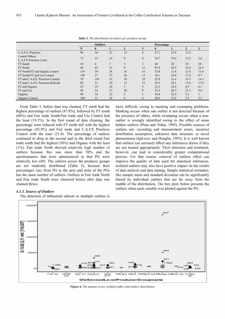
4.3.3. Source of Outliers
The detection of influential subsets or multiple outliers is
more difficult, owing to masking and swamping problems.
Masking occurs when one outlier is not detected because of
the presence of others, while swamping occurs when a non-
outlier is wrongly identified owing to the effect of some
hidden outliers (Pena and Yohai, 1995). Possible sources of
outliers are: recording and measurement errors, incorrect
distribution assumption, unknown data structure, or novel
phenomenon (Iglewicz and Hoaglin, 1993). It is well known
that outliers can seriously affect any inferences drawn if they
are not treated appropriately. Their detection and treatment,
however, can lead to considerably greater computational
process. For that reason, removal of outliers effect can
improve the quality of data used for statistical inferences.
Isolated outliers may also have positive impact on the results
of data analysis and data mining. Simple statistical estimates,
like sample mean and standard deviation can be significantly
biased by individual outliers that are far away from the
middle of the distribution. The box plots below presents the
outliers when each variable was plotted against the PG.
Figure 6. The amount of not certified coffee sold outliers distribution.
American Journal of Theoretical and Applied Statistics 2015; 4(6): 446-463 456
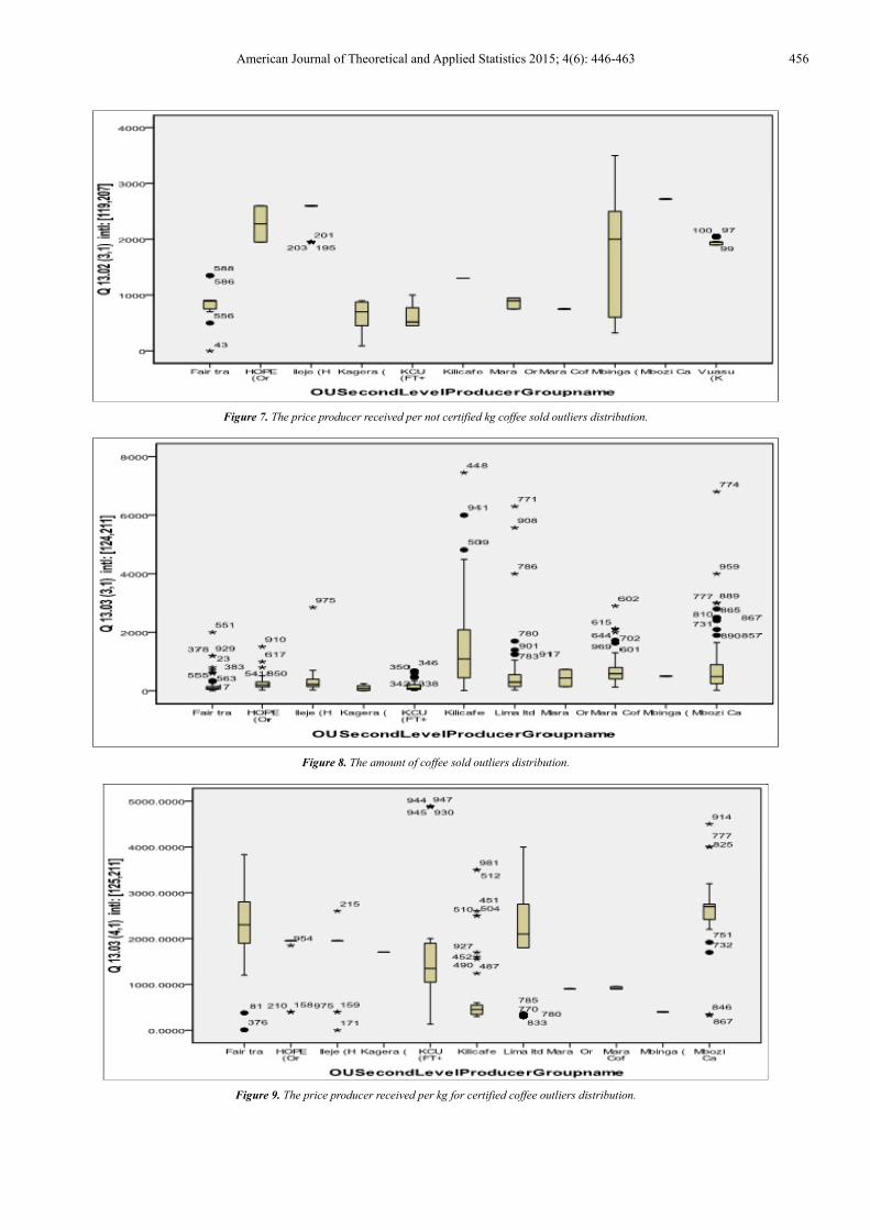
Figure 7. The price producer received per not certified kg coffee sold outliers distribution.
Figure 8. The amount of coffee sold outliers distribution.
Figure 9. The price producer received per kg for certified coffee outliers distribution.
457 Charles Kipkorir Masson: An Assessment of Farmers Livelihood in the Coffee Certification Schemes in Tanzania
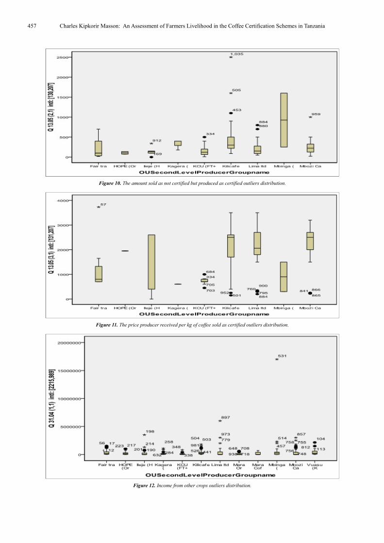
Figure 10. The amount sold as not certified but produced as certified outliers distribution.
Figure 11. The price producer received per kg of coffee sold as certified outliers distribution.
Figure 12. Income from other crops outliers distribution.

American Journal of Theoretical and Applied Statistics 2015; 4(6): 446-463 458
The amount of coffee sold had the highest number of
outliers(43), followed by income from other crops(37) and
the amount of coffee sold as not certified but were produced
as certified(9). All the 7 variables except kg coffee sold had 0
entries. Income from other crops had both the highest number
of extreme high values and the highest number of zeros (216).
The distribution of the outliers across the producer groups
were random and on the basis of these results, the most
appropriate data cleaning procedure is perform cleaning
twice because after the second round the mean and sample
size are reduced. Sample size reduced by 127 which means
we are likely to lose many observations in the subsequent
cleaning. Since this was secondary data, it is difficult to
verify whether the extreme values were really outliers or that
was the real data that the farmer gave.
4.4. Comparison of the Producer Groups
To compare the two groups, certified and non-certified, we
tested the hypothesis that;
H0: Both the certified and non-certified farmers have the
same income
H1:Their income is different
Significance level: a=0.05; Rejection region: We reject the
null hypothesis if p-value≤0.05
Table 6. Comparison of certification type income per indicator.
Total crop
revenue Revenue_ha
Block_income_revenue_all_ta
rget_crop_revenue
Coffe_reveue
_per_ha
Price_un
cert
Price_cert_
sold_uncert
Average_price_a
ll_coffee_sold
Mann-Whitney U 111871.5 95496 121048.5 117979.5 12116 881 111279.5
Wilcoxon W 239131.5 200149 259123.5 224009.5 87971 4284 215475.5
Z -0.65 -4.2 -0.51 -0.16 -9.09 -2.3 -2.1
Asymp. Sig. (2-
tailed) 0.52 0 0.61 0.87 0.02 0.04
Asymp. Sig. (1-
tailed) 0.26 0 0.3 0.44 0 0.01 0.02
One-tailed p-values ≤ the specified α=0.05, we reject the
null hypothesis that both the certified and non-certified
farmers have the same income and conclude that there exist a
significant difference in the income of the two certification
types.
To compare the 12 producer groups, we tested the
hypothesis that
H0: All the producer groups have the same income
H1: At least of the producer group income is different.
Significance level: a=0.05; Rejection region: Reject the
null hypothesis if p-value ≤ 0.05
Table 7. Comparison of the producer groups income per indicator.
Total crop
revenue Revenue_ha
Block_income_revenue_al
l_target_crop_revenue
Coffe_reveue
_per_ha
Price_unc
ert
Price_cert_
sold_uncert
Average_price_a
ll_coffee_sold
Chi-Square 484.94 479.55 465.67 496 318.45 56.34 543.14
df 11 11 11 11 9 9 11
Asymp. Sig 0 0 0 0 0 0 0
Since p-value=0 for all indicators ≤ 0.05=a, we reject the
null hypothesis and conclude that at α=0.05 level of
significance, there exist enough evidence to conclude that
there is a difference among the producer groups based on
their income.
Figure 13. Variations in block income for the certified and certified farmers.
459 Charles Kipkorir Masson: An Assessment of Farmers Livelihood in the Coffee Certification Schemes in Tanzania
These results shows that there exist two categories of
income earned by the farmers, which are distributed across
the two certification types (Figure 13). The categories are
those who earned below Tsh 60,000 and those earn above Tsh
60,000. C.A.F.E practices control Mbozi and FT/ C.A.F.E
practices control are non-certified yet their block income is
highest (both above Tsh 100000).FT South which certified
had the lowest block income. Organic and Organic control
had equal block income yet they belong to different
certification type. This suggests that there are likely other
factors that have contributed to the rise in farmers income, or
that when certification programs were initiated the farmers
were already established and they intervention, their impacts
were negligible.
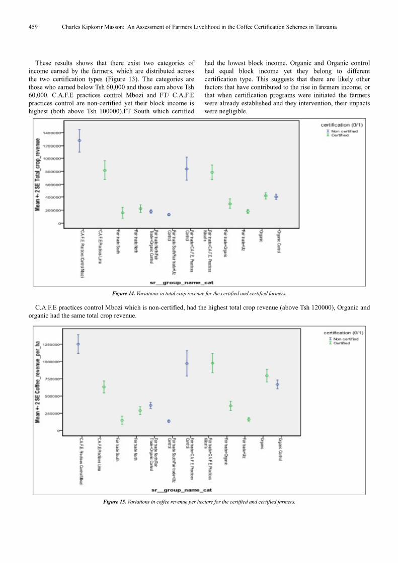
Figure 14. Variations in total crop revenue for the certified and certified farmers.
C.A.F.E practices control Mbozi which is non-certified, had the highest total crop revenue (above Tsh 120000), Organic and
organic had the same total crop revenue.
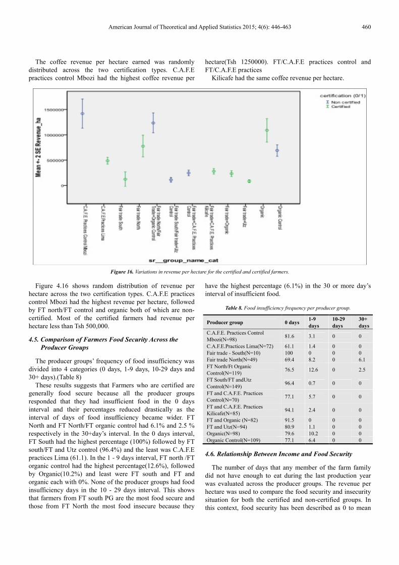
Figure 15. Variations in coffee revenue per hectare for the certified and certified farmers.
American Journal of Theoretical and Applied Statistics 2015; 4(6): 446-463 460
The coffee revenue per hectare earned was randomly
distributed across the two certification types. C.A.F.E
practices control Mbozi had the highest coffee revenue per
hectare(Tsh 1250000). FT/C.A.F.E practices control and
FT/C.A.F.E practices
Kilicafe had the same coffee revenue per hectare.
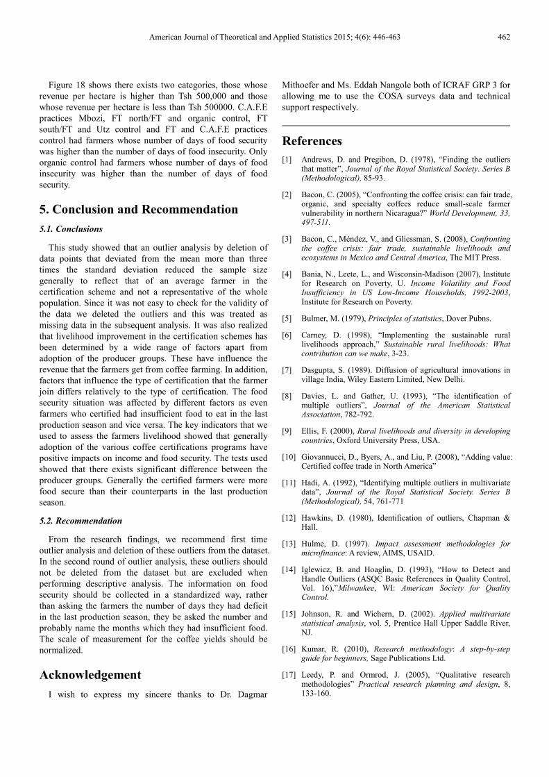
Figure 16. Variations in revenue per hectare for the certified and certified farmers.
Figure 4.16 shows random distribution of revenue per
hectare across the two certification types. C.A.F.E practices
control Mbozi had the highest revenue per hectare, followed
by FT north/FT control and organic both of which are non-
certified. Most of the certified farmers had revenue per
hectare less than Tsh 500,000.
4.5. Comparison of Farmers Food Security Across the
Producer Groups
The producer groups’ frequency of food insufficiency was
divided into 4 categories (0 days, 1-9 days, 10-29 days and
30+ days).(Table 8)
These results suggests that Farmers who are certified are
generally food secure because all the producer groups
responded that they had insufficient food in the 0 days
interval and their percentages reduced drastically as the
interval of days of food insufficiency became wider. FT
North and FT North/FT organic control had 6.1% and 2.5 %
respectively in the 30+day’s interval. In the 0 days interval,
FT South had the highest percentage (100%) followed by FT
south/FT and Utz control (96.4%) and the least was C.A.F.E
practices Lima (61.1). In the 1 - 9 days interval, FT north /FT
organic control had the highest percentage(12.6%), followed
by Organic(10.2%) and least were FT south and FT and
organic each with 0%. None of the producer groups had food
insufficiency days in the 10 - 29 days interval. This shows
that farmers from FT south PG are the most food secure and
those from FT North the most food insecure because they
have the highest percentage (6.1%) in the 30 or more day’s
interval of insufficient food.
Table 8. Food insufficiency frequency per producer group.
Producer group 0 days 1-9
days
10-29
days
30+
days
C.A.F.E. Practices Control
Mbozi(N=98) 81.6 3.1 0 0
C.A.F.E.Practices Lima(N=72) 61.1 1.4 0 0
Fair trade - South(N=10) 100 0 0 0
Fair trade North(N=49) 69.4 8.2 0 6.1
FT North/Ft Organic
Control(N=119) 76.5 12.6 0 2.5
FT South/FT andUtz
Control(N=149) 96.4 0.7 0 0
FT and C.A.F.E. Practices
Control(N=70) 77.1 5.7 0 0
FT and C.A.F.E. Practices
Kilicafe(N=85) 94.1 2.4 0 0
FT and Organic (N=82) 91.5 0 0 0
FT and Utz(N=94) 80.9 1.1 0 0
Organic(N=98) 79.6 10.2 0 0
Organic Control(N=109) 77.1 6.4 0 0
4.6. Relationship Between Income and Food Security
The number of days that any member of the farm family
did not have enough to eat during the last production year
was evaluated across the producer groups. The revenue per
hectare was used to compare the food security and insecurity
situation for both the certified and non-certified groups. In
this context, food security has been described as 0 to mean

461 Charles Kipkorir Masson: An Assessment of Farmers Livelihood in the Coffee Certification Schemes in Tanzania
the days of food insufficiency and 1 means the days of sufficiency as described (Figure 17 and Figure 18).
Figure 17. Variations in revenue per hectare for certified farmers who are food secure and those who are not. Producer groups displayed separately; error
bars represents 2 times the standard error.
Figure 17 shows that FT and Utz had the same number of
farmers who responded that the number of days of food
security were equal to the number of days of food insecurity.
C.A.F.E practices Lima, FT north FT and C.A.F.E practices
Kilicafe had the farmers whose number of days of food
security were higher than the days of food insecurity. Ft and
organic and organic each had farmers whose number of food
insecurity were higher than the number of food security.
None of the farmers from FT south were food insecure.
Figure 18. Variations in revenue per hectare for non-certified farmers who are food secure and those who are not. Producer groups displayed separately;
error bars represents 2 times the standard error.
American Journal of Theoretical and Applied Statistics 2015; 4(6): 446-463 462
Figure 18 shows there exists two categories, those whose
revenue per hectare is higher than Tsh 500,000 and those
whose revenue per hectare is less than Tsh 500000. C.A.F.E
practices Mbozi, FT north/FT and organic control, FT
south/FT and Utz control and FT and C.A.F.E practices
control had farmers whose number of days of food security
was higher than the number of days of food insecurity. Only
organic control had farmers whose number of days of food
insecurity was higher than the number of days of food
security.
5. Conclusion and Recommendation
5.1. Conclusions
This study showed that an outlier analysis by deletion of
data points that deviated from the mean more than three
times the standard deviation reduced the sample size
generally to reflect that of an average farmer in the
certification scheme and not a representative of the whole
population. Since it was not easy to check for the validity of
the data we deleted the outliers and this was treated as
missing data in the subsequent analysis. It was also realized
that livelihood improvement in the certification schemes has
been determined by a wide range of factors apart from
adoption of the producer groups. These have influence the
revenue that the farmers get from coffee farming. In addition,
factors that influence the type of certification that the farmer
join differs relatively to the type of certification. The food
security situation was affected by different factors as even
farmers who certified had insufficient food to eat in the last
production season and vice versa. The key indicators that we
used to assess the farmers livelihood showed that generally
adoption of the various coffee certifications programs have
positive impacts on income and food security. The tests used
showed that there exists significant difference between the
producer groups. Generally the certified farmers were more
food secure than their counterparts in the last production
season.
5.2. Recommendation
From the research findings, we recommend first time
outlier analysis and deletion of these outliers from the dataset.
In the second round of outlier analysis, these outliers should
not be deleted from the dataset but are excluded when
performing descriptive analysis. The information on food
security should be collected in a standardized way, rather
than asking the farmers the number of days they had deficit
in the last production season, they be asked the number and
probably name the months which they had insufficient food.
The scale of measurement for the coffee yields should be
normalized.
Acknowledgement
I wish to express my sincere thanks to Dr. Dagmar
Mithoefer and Ms. Eddah Nangole both of ICRAF GRP 3 for
allowing me to use the COSA surveys data and technical
support respectively.
References
[1] Andrews, D. and Pregibon, D. (1978), “Finding the outliers that matter”, Journal of the Royal Statistical Society. Series B (Methodological), 85-93.
[2] Bacon, C. (2005), “Confronting the coffee crisis: can fair trade, organic, and specialty coffees reduce small-scale farmer vulnerability in northern Nicaragua?” World Development, 33, 497-511.
[3] Bacon, C., Méndez, V., and Gliessman, S. (2008), Confronting the coffee crisis: fair trade, sustainable livelihoods and ecosystems in Mexico and Central America, The MIT Press.
[4] Bania, N., Leete, L., and Wisconsin-Madison (2007), Institute for Research on Poverty, U. Income Volatility and Food Insufficiency in US Low-Income Households, 1992-2003, Institute for Research on Poverty.
[5] Bulmer, M. (1979), Principles of statistics, Dover Pubns.
[6] Carney, D. (1998), “Implementing the sustainable rural livelihoods approach,” Sustainable rural livelihoods: What contribution can we make, 3-23.
[7] Dasgupta, S. (1989). Diffusion of agricultural innovations in village India, Wiley Eastern Limited, New Delhi.
[8] Davies, L. and Gather, U. (1993), “The identification of multiple outliers”, Journal of the American Statistical Association, 782-792.
[9] Ellis, F. (2000), Rural livelihoods and diversity in developing countries, Oxford University Press, USA.
[10] Giovannucci, D., Byers, A., and Liu, P. (2008), “Adding value: Certified coffee trade in North America”
[11] Hadi, A. (1992), “Identifying multiple outliers in multivariate data”, Journal of the Royal Statistical Society. Series B (Methodological), 54, 761-771
[12] Hawkins, D. (1980), Identification of outliers, Chapman & Hall.
[13] Hulme, D. (1997). Impact assessment methodologies for microfinance: A review, AIMS, USAID.
[14] Iglewicz, B. and Hoaglin, D. (1993), “How to Detect and Handle Outliers (ASQC Basic References in Quality Control, Vol. 16),”Milwaukee, WI: American Society for Quality Control.
[15] Johnson, R. and Wichern, D. (2002). Applied multivariate statistical analysis, vol. 5, Prentice Hall Upper Saddle River, NJ.
[16] Kumar, R. (2010), Research methodology: A step-by-step guide for beginners, Sage Publications Ltd.
[17] Leedy, P. and Ormrod, J. (2005), “Qualitative research methodologies” Practical research planning and design, 8, 133-160.
463 Charles Kipkorir Masson: An Assessment of Farmers Livelihood in the Coffee Certification Schemes in Tanzania
[18] Lewis, J. (2005), “Strategies for survival: Migration and fair trade-organic coffee production in Oaxaca, Mexico,”The Center for Comparative Immigration Studies, Working Paper.
[19] Martincic, F. and Schwiebert, L. (2006), “Distributed event detection in sensor networks”, in Systems and Networks Communications, 2006. ICSNC'06. International Conference on, IEEE, pp. 43-43.
[20] Mayne, R., Tola, A., and Kebede, G. (2002), “Crisis in the birth place of coffee”, Oxfam International research paper, Oxfam International.
[21] Pena, D. and Yohai, V. (1995). “The detection of influential subsets in linear regression by using an influence matrix”, Journal of the Royal Statistical Society. Series B (Methodological), 145-156.
[22] Ponte, S. (2004a), “The politics of ownership: Tanzanian coffee policy in the age of liberal reformism”, African Affairs, 103, 615.
[23] Ponte, S. (2004b), “Standards and sustainability in the coffee sector”, International Institute for Sustainable Development. Available at http://www. iisd. org.
[24] Ravallion, M. (2003), “Assessing the poverty impact of an assigned program”, The impact of economic policies on poverty and income distribution: evaluation techniques and tools, 103-22.
[25] Raynolds, L. (2002), Poverty alleviation through participation in Fair Trade coffee networks: existing research and critical issues, Ford Foundation.
[26] Read, R. (1999), “Detecting outliers in non-redundant diffraction data”, Acta Crystallographica Section D: Biological Crystallography, 55, 1759-1764.
[27] Wollni, M. and Zeller, M. (2007). “Do farmers bene_t from participating in specialty markets and cooperatives? The case of coffee marketing in Costa Rica1”, Agricultural Economics, 37, 243-248.
Recommended