Download pdf - An Analysis of the Underground Economy and its … · · 2012-11-16evade taxes by operating in the underground economy. ... explanations for why entrepreneurs go underground (See

- 1 -

1We would like to thank Mohammad Arzaghi, Mohsin Khan, Anwar Shah, Shahid Yusuf, and Shang-Jin Wei for many helpful suggestions. The views expressed here are those of the authors and do not necessarily reflect the opinions of the International Monetary Fund.

An Analysis of the Underground Economy and its Macroeconomic Consequences

ByEra Dabla-Norris

andAndrew Feltenstein1

International Monetary Fund

Abstract

This paper develops a dynamic general equilibrium model in which optimizing agentsevade taxes by operating in the underground economy. The cost to firms of evading taxesis that they find themselves subject to credit rationing from banks. Our model simulationsshow that in the absence of budgetary flexibility to adjust expenditures, raising tax ratestoo high drives firms into the underground economy, thereby reducing the tax base.Aggregate investment in the economy is lowered because of credit rationing. Taxes thatare too low eliminate the underground economy, but result in unsustainable budget andtrade deficits. Thus, the optimal rate of taxation, from a macroeconomic point of view,may lead to some underground activity.

JEL Classification: H26; E26; C68

Keywords: Underground economy, macroeconomic performance, credit rationing

Authors E-Mail Addresses: [email protected]; [email protected]

mailto:[email protected];

mailto:[email protected]

- 2 -

2 As in Braun and Loayza (1993), the underground economy is defined as a set of economicunits which do not comply with one or more government imposed taxes and regulations, butwhose production is considered legal”.

I. INTRODUCTION

In many developing and transition countries, economic activity in the

underground economy is estimated in excess of 40 percent of GDP (Schneider and Enste

(2000), Friedman et. al (2000)).2 Heavy tax burdens and excessive regulation imposed by

governments that lack the capability to enforce compliance are widely regarded as

driving firms into the underground economy. This diversion into unofficial activity

undermines the tax base and can significantly affect public finances and the quality of

public administration (Loayza (1996), Johnson et al. (1997), Dessy and Pallage (2003)).

The illegal nature of underground activity also constrains private investment and growth.

For instance, firms operating underground are often unable to make use of market-

supporting institutions like the judicial system and courts and, as a result, may

underinvest (De Soto (1989)). One important cost imposed by the inability to enforce

legal contracts is the limited access to formal credit markets.

In this paper, we develop a simple intertemporal general equilibrium model with

heterogeneous agents and credit rationing to explain the prevalence of large underground

economies in many developing and transition countries. In particular, we explore the link

between tax rates, access to credit, and the size of the underground economy and

examines the consequences of the underground economy for public finances and

aggregate economic performance. Entry and exit into the underground economy is

derived as part of optimizing behavior that depends on taxes and interest rates. Firms

- 3 -

3 In their study of private manufacturing firms in transition countries, Johnson et. al (2000)find that the availability of loans from the banking system was greater in Eastern Europeancountries with small underground economies, such as Poland , than in countries with largehidden activity, such as Ukraine and Russia.

operating underground are subject to credit rationing by banks which reduce loans in

relation to the firm’s nonpayment of taxes. This assumption is consistent with the

observation that it may be more difficult for tax evaders to borrow from a bank because

to do so would require official documentation, especially if the bank requires collateral

and if the process of hiding economic activity involves concealing the true ownership of

assets.3

Since the size of the underground economy in the paper depends upon both

endogenous and exogenous variables, our framework has scope for policy changes. In

particular, we address the issue of policy responses towards the emergence of

underground activity and emphasize the ambiguous effects of taxation by means of

numerical simulations for Pakistan. This should be viewed as an illustrative example of a

developing country which faces problems from tax evasion and parallel markets for both

goods and financial assets. Economic reform will depend upon policies that reduce the

various forms of tax evasion, especially given the typical developing country’s

difficulties with controlling its budget deficit.

There have been a number of empirical studies of the scope of the underground

economy in developing countries (see Schnieder and Enste (2000) for a survey). Most of

these studies use proxies, such as the amount of cash in circulation, or electricity

consumption to estimate the size of the underground economy. In addition, they are not

derived from optimizing models, but are based upon ad hoc empiricism. Accordingly,

- 4 -

3 Johnson et al. (1998, 2000) find that a high corporate tax burden combined withineffective and discretionary application of the tax system and other regulationsinfluences the size of the underground economy. Djankov et. al (2002) find evidence ofsignificant “entry costs” in the form of registration and license fees in the formaleconomy. Such costs range from a low of 2 procedures, taking two days and generating acost equivalent to 2.3 percent of GDP per capita in Canada, to a high of 21 procedures,80 days and 463 percent of GDP per capita in the Dominican Republic.

5 Burgess and Stern (1993) note that in developing countries, corporate income taxesrepresent 17.8 percent of total tax revenues as opposed to 7.6 percent in industrializedcountries.

they can at best be used for partial equilibrium analysis and hence may lead to inaccurate

conclusions.

Section II provides a brief overview of our modeling of the underground economy.

Section III presents our dynamic general equilibrium model. Section IV discusses the

parameterization of the model and presents the simulation results. Section V concludes.

II. MACROECONOMIC BACKGROUND

High statutory tax rates and onerous official regulations are widely cited as

explanations for why entrepreneurs go underground (See de Soto (1989), Friedman et al

(2000), Johnson et. al (1998), among others). Following this literature, our paper also

models the benefits from operating in terms of the firm’s desire to evade corporate taxes.4

This assumption is consistent with the observation that in many developing countries,

taxes on formal firms constitute a major source of government revenues, and narrow tax

bases for formal firms have often resulted in governments imposing very high marginal

tax rates.5

The cost of operating in the underground economy is modeled in terms of the

- 5 -

6 Straub (2003) develops a partial equilibrium model of firm’s choice between formalityand informality with dual credit markets, credit rationing, and a cost of entry intoformality. Our paper examines the interaction between the decision to operate formallyand the availability of formal credit in a general equilibrium setting and considers theeffect on growth.

inability to borrow from the official banking system.6 Banks in the model are assumed

not to have perfect information about the firm’s true ownership of assets and its

associated true tax obligation. We assume that due to collateral requirements credit is

provided only in relation to the firm’s implied ownership of assets, which is determined

from its actual tax payment. The idea here is that in the face of default, banks can only

seize those assets that have been officially declared by the firm. Hence, the higher the

extent of tax evasion, the lower the implied value of firm assets, and the lower the

amount of credit provided by the banking system. Our approach has some similarity to

Kiyotaki and Moore (1997) who model credit limits on loans. These limits are

determined by estimates of collateral which, in turn, are determined by estimates of

durable asset holdings by borrowers. Here, tax payments are used to estimate the value of

the durable asset of the borrower, as the asset cannot be directly observed.

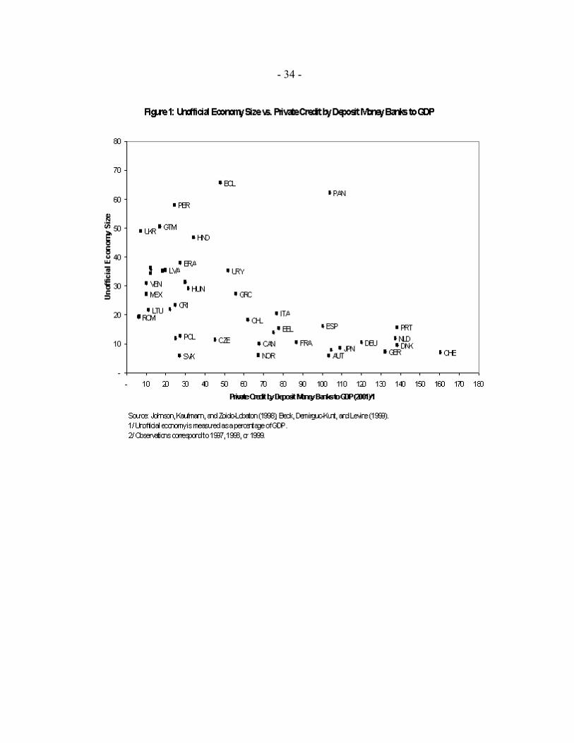
Figure 1 indicates the relationship between the size of the underground economy

and the ratio of private sector credit to GDP, which is widely regarded as a measure of

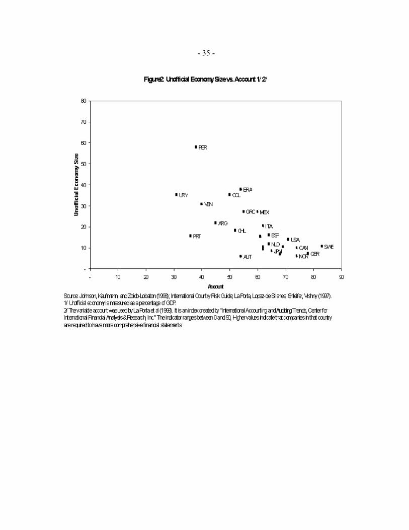
liquidity in the economy, for a cross-section of countries. The relationship between the

relative size of the underground activity and the extent to which companies are required

to provide comprehensive financial statements is reported in Figure 2. Taken together,

these suggest an inverse relationship between the size of the underground economy and

the availability of private sector credit and accounting standards and provide some

- 6 -

7Using a firm-level data set for 48 countries, Straub (2003) finds that once size andindividual characteristics of firms are accounted for, the efficiency of credit markets has asignificant effect on the degree of formality of firms.

8Huq and Sultan (1991) note that in Bangladesh, while borrowing rates from commercialbanks were around 12 percent, firms dependent on noninstitutional sources to meet theirfinancing needs paid rates between 48 to 100 percent. McMillan and Woodruff (1999)examine the role informal relationships such as trade credits rather than banks play inmeeting financing needs of firms in Vietnam. However, they do not examine the linksbetween informal trading relationships and underground activity.

6 Sarte (2000) develops a model which examines the link between the size of the informaleconomy and corrupt bureaucracies. He shows that in the presence of a corruptbureaucracy, it may be efficient to locate economic activity in the informal economy if thecosts of informality are low. However, he ignores credit rationing by banks.

justification for the assumption of credit rationing in the paper.7

We assume that firms can operate partially in the formal and partially in the

underground economy. That part of their operation that takes place in the legal economy

pays taxes and can borrow from the banking system. That part that is underground does

not pay taxes and cannot borrow. Admittedly this distinction is artificial, but captures

some of the benefits and costs of operating in the underground economy discussed in the

literature. In reality, the underground firm may still be able to finance its investment

needs by relying on trade credits or borrowing from secondary lenders who charge higher

than market interest rates and are willing to incur high risks.8 Presumably, in the absence

of legal enforcement of contracts and inadequate or weak business networks and supplier

relationships, this would further increase the costs of operating underground.

We ignore the effects of corruption in generating an underground economy.9

Presumably, the size of the underground economy may itself serve as a proxy for the

extent of corruption in the economy. This might be appropriate if the country in question

has relatively low statutory tax rates, so the incentives to evade taxes would not exist

- 7 -

unless doing so were not easy. Alternatively, a large underground economy can be a

result of firms seeking to escape a predatory bureaucracy in the formal economy (Shleifer

(1997), Johnson et al. (1998)). Of course, the presence of a large underground economy

could indicate high costs of ensuring compliance rather than corrupt officials.

Our approach also assumes that firms can evade taxes without any real risk of

detection or punishment. From a modeling perspective, it is difficult to determine just

what the penalty for tax evasion should be. That is, should it be a criminal penalty or a

fine? Should it be proportional to the size of the tax evasion, or should it be a flat rate? In

addition, what is the probability of apprehension faced by a tax evader? Presumably this

probability should itself be some function of the enforcement technology, the amount of

evasion, as well as the amount of money spend on enforcement. A problem with that

modeling strategy is that, as there is no clear mapping from the enforcement technology

and how spending affects the probability of being caught to real data, it does not offer a

reasonable framework for quantitative evaluations. Moreover, Shleifer and Vishny

(1993) point out that where public pressure on corruption or the enforcement ability of

the government is relatively weak - as we believe to be the case in many developing

countries - this is in fact a fitting assumption.

In our model, the decision to operate in the underground economy depends on the

firm’s present value of the future stream of returns on marginal investment relative to the

return on the corporate capital tax rate. If the marginal rate of return is higher than the

corporate tax rate, the firm chooses to operate in the above ground economy, since it is

profitable to borrow and pay taxes. If, on the other hand, the tax rate is greater than the

marginal rate of return on investment, the firm chooses to operate in the underground

- 8 -

economy. However, we assume that the firm does not make a bipolar choice. That is, it

reduces its tax payments and borrowing for investment proportionally to the difference

between the rate of return and the tax rate. Hence if the rate of return were 0, then the

firm would pay no taxes and carry out no borrowing for investment. If tax rates and rates

of return on investment are equal, then the firm pays the full tax rate and invests.

In this framework, one could measure the size of the underground economy by

aggregating the value of all lost tax revenues and comparing it to the revenues that would

accrue if rates were low enough so as to generate no underground activity. The ratio of

the two would then provide a measure of the share of the underground economy in total

economic activity. We would thus compare two simulated equilibria.

III. A GENERAL EQUILIBRIUM SPECIFICATION

In this section we develop the formal structure of a dynamic general equilibrium

model that endogenously generates an underground economy. Much of the structure of

our model is designed to permit numerical implementation. Our model has n discrete

time periods. All agents optimize in each period over a 2 period time horizon. That is, in

period t they optimize given prices for periods and and expectations for prices for

the future after . When period arrives, agents reoptimize for period and

, based on new information about period .

Our model structure is related to a number of earlier papers, starting with Strotz

(1956). Here preferences are inconsistent over time, primarily because the future does not

turn out as anticipated. Thus it may be optimal for agents to commit themselves for a few

periods into the future. They may be better off, however, if they reoptimize at some later

- 9 -

10 We could have any number of capital types without affecting the structure of the model.

11 We assume that the labor market is not segmented and there is no wage differential betweenworkers in the underground and the formal economy.

date, based on their own changed preferences or changes in economic variables. This is

quite different from the notion of time inconsistency of Kydland and Prescott (1977),

where rational behavior by economic agents itself leads to inconsistencies in what would

otherwise be an optimal government plan.

1. Production

There are 8 factors of production and 3 types of financial assets:

1-5 Capital types 9. Domestic currency6. Urban labor 10. Bank deposits7. Rural labor 11. Foreign currency8. Land

The five types of capital correspond to five aggregate nonagricultural productive

sectors.10 An input-output matrix, At, is used to determine intermediate and final

production in period t. Corresponding to each sector in the input-output matrix, sector-

specific value added is produced using capital and urban labor for the nonagricultural

sectors, and land and rural labor in agriculture.

Assuming that there are more than five sectors in the economy, the different

factors would be allocated across the economy so that agriculture uses land and rural

labor, and all other sectors use one of the five capital types plus urban labor.

Accordingly, capital is perfectly mobile across a given subsector, but is immobile across

other subsectors. Labor, on the other hand, may migrate from the rural to the urban

sector.11

- 10 -

12 We assume that all foreign borrowing for investment is carried out by the government, sothat, implicitly, the government is borrowing for the private investor but the debt incurred ispublicly guaranteed.

(1)

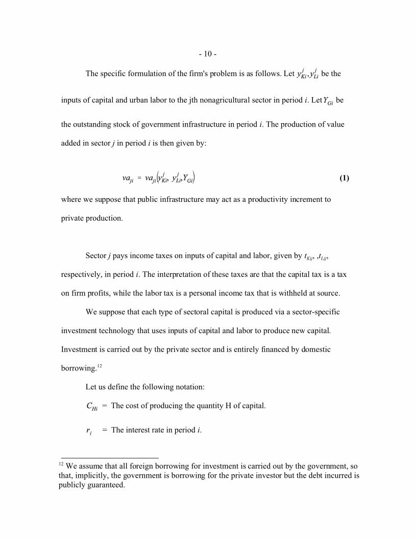
The specific formulation of the firm's problem is as follows. Let , be the

inputs of capital and urban labor to the jth nonagricultural sector in period i. Let be

the outstanding stock of government infrastructure in period i. The production of value

added in sector j in period i is then given by:

where we suppose that public infrastructure may act as a productivity increment to

private production.

Sector j pays income taxes on inputs of capital and labor, given by tKij, ,tLij,

respectively, in period i. The interpretation of these taxes are that the capital tax is a tax

on firm profits, while the labor tax is a personal income tax that is withheld at source.

We suppose that each type of sectoral capital is produced via a sector-specific

investment technology that uses inputs of capital and labor to produce new capital.

Investment is carried out by the private sector and is entirely financed by domestic

borrowing.12

Let us define the following notation:

= The cost of producing the quantity H of capital.

= The interest rate in period i.

- 11 -

13 In reality, we can regard the tax rate on capital as the generalized tax rate, includingtaxation, regulation, and corruption (bribes).

(2)

= The return to capital in period i.

= The price of money in period i.

= The rate of depreciation of capital.

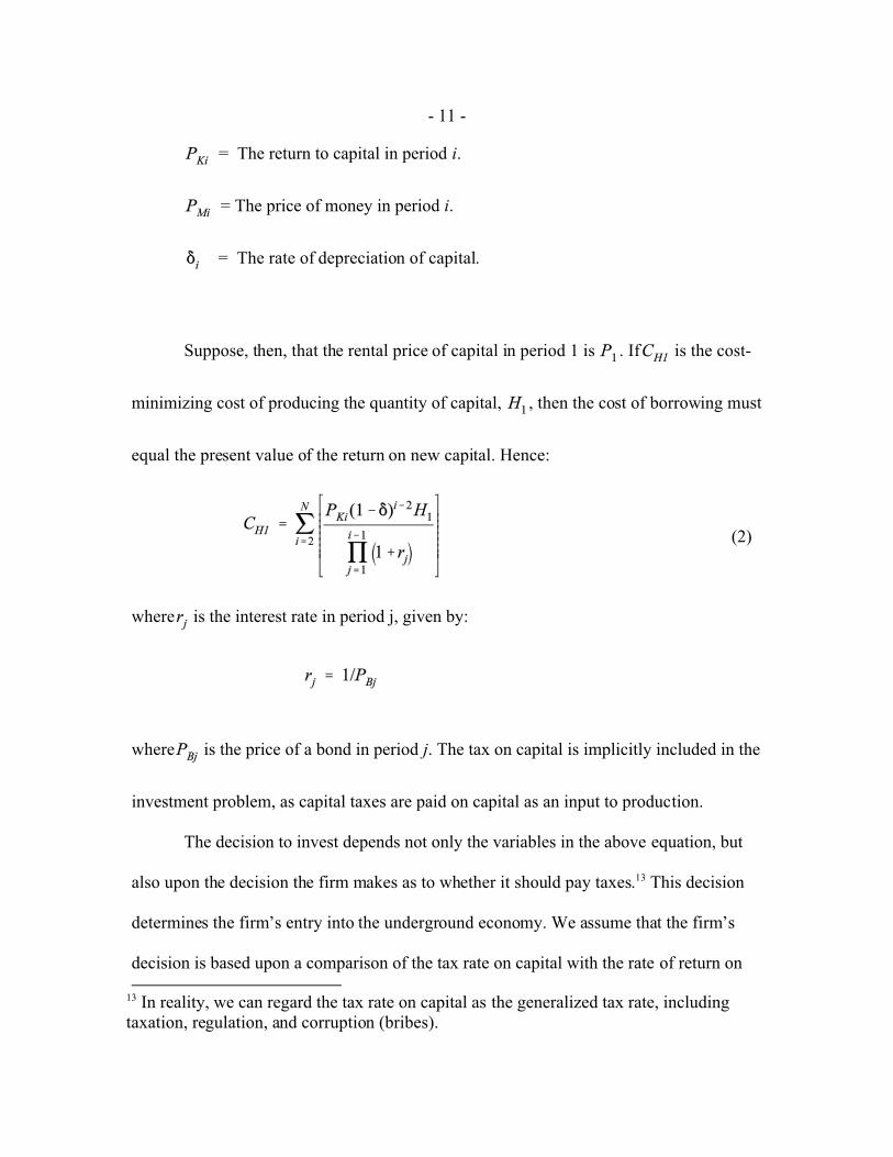
Suppose, then, that the rental price of capital in period 1 is . If is the cost-

minimizing cost of producing the quantity of capital, , then the cost of borrowing must

equal the present value of the return on new capital. Hence:

where is the interest rate in period j, given by:

where is the price of a bond in period j. The tax on capital is implicitly included in the

investment problem, as capital taxes are paid on capital as an input to production.

The decision to invest depends not only the variables in the above equation, but

also upon the decision the firm makes as to whether it should pay taxes.13 This decision

determines the firm’s entry into the underground economy. We assume that the firm’s

decision is based upon a comparison of the tax rate on capital with the rate of return on

- 12 -

14 Clearly this is an ad hoc assumption. We wish to capture the notion that the decisionwhether or not to pay taxes is based on the relationship between the return to investment andthe tax rate on capital.

new capital. If the tax rate on capital is less than the corresponding rate of return, the firm

pays the full tax. If the tax rate is greater than the return to new capital, then the firm pays

less than the full capital tax. That is, it withdraws, at least partially, into the underground

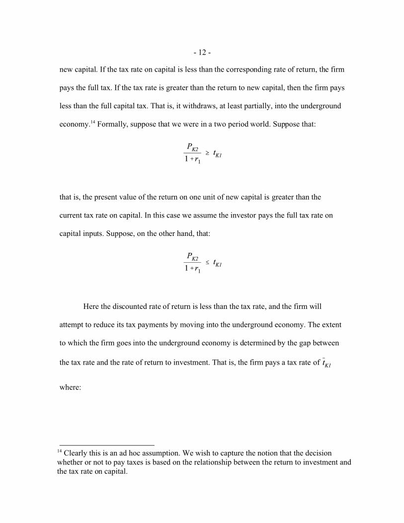
economy.14 Formally, suppose that we were in a two period world. Suppose that:

that is, the present value of the return on one unit of new capital is greater than the

current tax rate on capital. In this case we assume the investor pays the full tax rate on

capital inputs. Suppose, on the other hand, that:

Here the discounted rate of return is less than the tax rate, and the firm will

attempt to reduce its tax payments by moving into the underground economy. The extent

to which the firm goes into the underground economy is determined by the gap between

the tax rate and the rate of return to investment. That is, the firm pays a tax rate of

where:

- 13 -

15 Here could be a function of the enforcement technology. In our model, however, we

assume that there is no enforcement technology or means to enforce tax compliance.

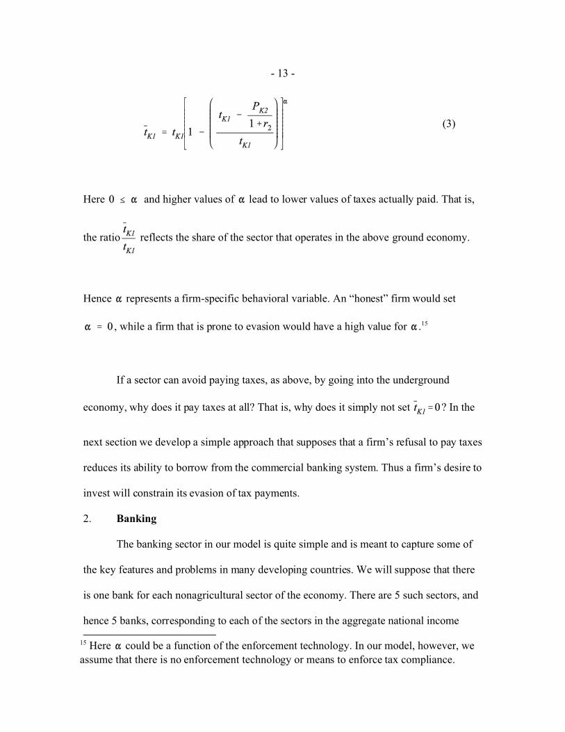
(3)

Here and higher values of lead to lower values of taxes actually paid. That is,

the ratio reflects the share of the sector that operates in the above ground economy.

Hence represents a firm-specific behavioral variable. An “honest” firm would set

, while a firm that is prone to evasion would have a high value for .15

If a sector can avoid paying taxes, as above, by going into the underground

economy, why does it pay taxes at all? That is, why does it simply not set ? In the

next section we develop a simple approach that supposes that a firm’s refusal to pay taxes

reduces its ability to borrow from the commercial banking system. Thus a firm’s desire to

invest will constrain its evasion of tax payments.

2. Banking

The banking sector in our model is quite simple and is meant to capture some of

the key features and problems in many developing countries. We will suppose that there

is one bank for each nonagricultural sector of the economy. There are 5 such sectors, and

hence 5 banks, corresponding to each of the sectors in the aggregate national income

- 14 -

accounts. Such sectoral specialization of the banking system reflects the reality of many

developing countries.

We contend that the underground economy affects different sectors in a non-

uniform way. Indeed, tax evasion in one sector may benefit the sector at a micro level but

may be harmful to the macro economy. Tax evasion varies across sectors not only

because of the behavior of firms in that sector, but also because different banks could

have varying attitudes towards lending to clients who have evaded taxes.

Each bank lends primarily to the sector with which it is associated. The banks are,

however, not fully specialized in the sector they correspond to. We make the simplifying

assumption that each bank holds a fixed share of the outstanding debt of its particular

sector. It then holds additional fixed shares of the debt of each of the remaining sectors.

We make this assumption of diversification of assets in order to allow for a situation in

which a firm that evades taxes, and thereby enters the underground economy, might

receive varying degrees of credit rationing from the different banks to which it applies

for loans.

We choose a simple approach to determine the degree of credit rationing that

firms face. Our premise is that banks have no direct way of knowing whether specific

firms operate in the underground economy. We assume that banks only care about the

amount of capital that they estimate the firm may have. If the firm defaults on its loan,

then this represents the best estimate of the amount that the bank could seize. The bank

would, presumably, be willing to lend an amount equal to at least the estimated firm

capital. If the firm requests a loan larger than its estimated capital, the bank may choose

to grant the full loan, or it may choose to restrict the loan amount. This restriction would

- 15 -

16 We have not explicitly incorporated bankruptcies and defaults in this model, for the sake ofsimplicity. However bankruptcies and corresponding bank contractions can be introduced asin Ball and Feltenstein (2001) and Blejer, Feldman, and Feltenstein (2002).

depend, in turn, upon the bank’s degree of risk aversion.

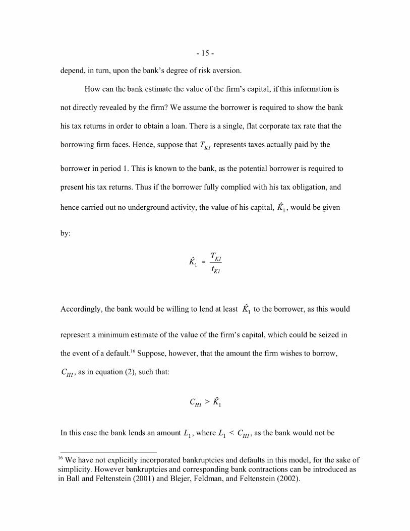
How can the bank estimate the value of the firm’s capital, if this information is

not directly revealed by the firm? We assume the borrower is required to show the bank

his tax returns in order to obtain a loan. There is a single, flat corporate tax rate that the

borrowing firm faces. Hence, suppose that represents taxes actually paid by the

borrower in period 1. This is known to the bank, as the potential borrower is required to

present his tax returns. Thus if the borrower fully complied with his tax obligation, and

hence carried out no underground activity, the value of his capital, , would be given

by:

Accordingly, the bank would be willing to lend at least to the borrower, as this would

represent a minimum estimate of the value of the firm’s capital, which could be seized in

the event of a default.16 Suppose, however, that the amount the firm wishes to borrow,

, as in equation (2), such that:

In this case the bank lends an amount , where , as the bank would not be

- 16 -

(4)

able to seize the full value of the loan in the case of a default. The situation we have

described would, in the case of perfect certainty, have credit rationing when the estimated

value of the firm’s capital is less than its loan request. If the firm’s capital is greater than

its loan request, there would be no credit rationing.

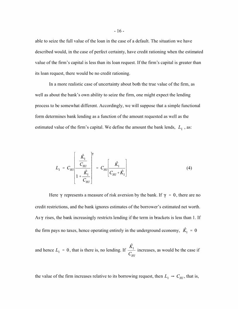
In a more realistic case of uncertainty about both the true value of the firm, as

well as about the bank’s own ability to seize the firm, one might expect the lending

process to be somewhat different. Accordingly, we will suppose that a simple functional

form determines bank lending as a function of the amount requested as well as the

estimated value of the firm’s capital. We define the amount the bank lends, , as:

Here represents a measure of risk aversion by the bank. If , there are no

credit restrictions, and the bank ignores estimates of the borrower’s estimated net worth.

As rises, the bank increasingly restricts lending if the term in brackets is less than 1. If

the firm pays no taxes, hence operating entirely in the underground economy,

and hence , that is there is, no lending. If increases, as would be the case if

the value of the firm increases relative to its borrowing request, then , that is,

- 17 -

the bank lends the full value of the request.

Thus if a firm operates entirely in the underground economy it will not be able to

borrow to finance investment. If banks are highly risk averse, they will never lend more

than a firm’s estimated net worth, which is based on its tax return. This tax return

therefore represents all the information the bank needs in order to determine its response

to a request for a loan.

- 18 -

17We use two consumer categories in order to correspond to available country dataclassifications, as described in the next section.

3. Consumption

There are two types of consumers, representing rural and urban labor.17 We

suppose that the two consumer classes have differing Cobb-Douglas demands. The

consumers also differ in their initial allocations of factors and financial assets.

The consumers maximize intertemporal utility functions, which have as

arguments the levels of consumption and leisure in each of the two periods. We permit

rural-urban migration which depends upon the relative rural and urban wage rate. The

consumers maximize these utility functions subject to intertemporal budget constraints.

The consumer saves by holding money, domestic bank deposits, and foreign currency.

He requires money for transactions purposes, but his demand for money is sensitive to

changes in the inflation rate. The consumer pays taxes on his consumption, and does not

have any direct contact with the underground economy. That is, he pays the full nominal

rates under all circumstances.

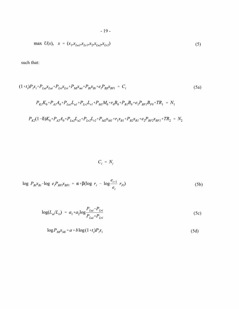
Here, and in what follows, we will use x to denote a demand variable and y to

denote a supply variable. In order to avoid unreadable subscripts, let 1 refer to period i

and 2 refer to period i +1. The consumer's maximization problem is thus:

- 19 -

(5)

(5a)

(5d)

(5b)

(5c)

such that:

- 20 -

(5e)

where:

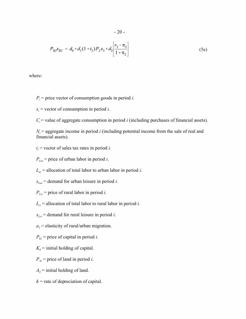
Pi = price vector of consumption goods in period i.

xi = vector of consumption in period i.

Ci = value of aggregate consumption in period i (including purchases of financial assets).

Ni = aggregate income in period i (including potential income from the sale of real andfinancial assets).

ti = vector of sales tax rates in period i.

PLui = price of urban labor in period i.

Lui = allocation of total labor to urban labor in period i.

xLui = demand for urban leisure in period i.

PLri = price of rural labor in period i.

Lri = allocation of total labor to rural labor in period i.

xLri = demand for rural leisure in period i.

a2 = elasticity of rural/urban migration.

PKi = price of capital in period i.

K0 = initial holding of capital.

PAi = price of land in period i.

A0 = initial holding of land.

* = rate of depreciation of capital.

- 21 -

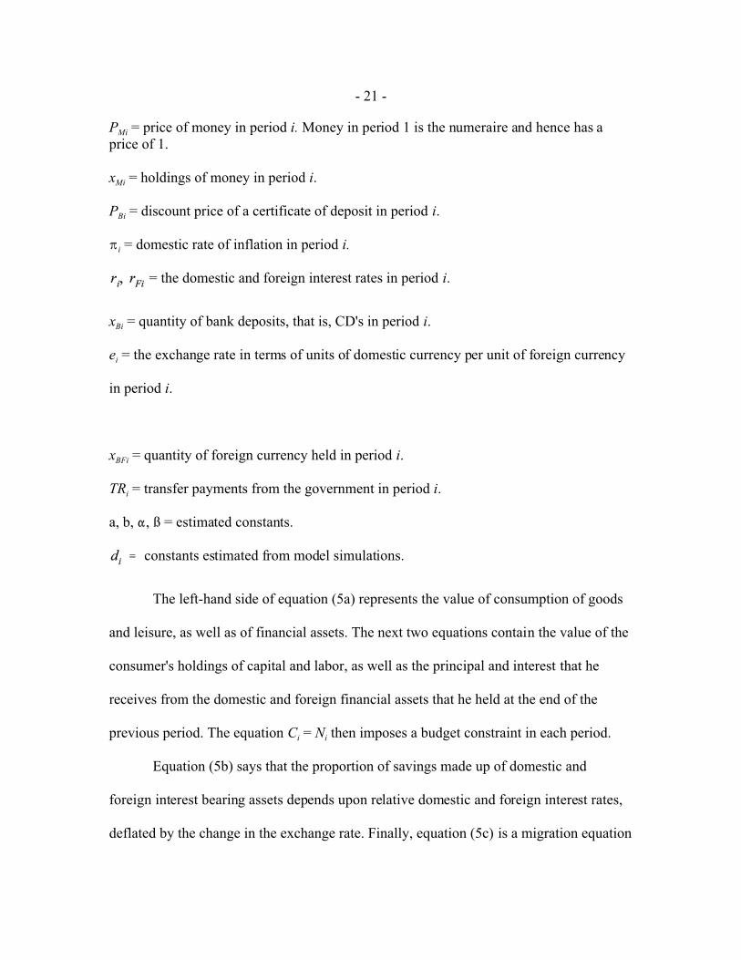
PMi = price of money in period i. Money in period 1 is the numeraire and hence has aprice of 1.

xMi = holdings of money in period i.

PBi = discount price of a certificate of deposit in period i.

B i = domestic rate of inflation in period i.

= the domestic and foreign interest rates in period i.

xBi = quantity of bank deposits, that is, CD's in period i.

ei = the exchange rate in terms of units of domestic currency per unit of foreign currency

in period i.

xBFi = quantity of foreign currency held in period i.

TRi = transfer payments from the government in period i.

a, b, ", ß = estimated constants.

constants estimated from model simulations.

The left-hand side of equation (5a) represents the value of consumption of goods

and leisure, as well as of financial assets. The next two equations contain the value of the

consumer's holdings of capital and labor, as well as the principal and interest that he

receives from the domestic and foreign financial assets that he held at the end of the

previous period. The equation Ci = Ni then imposes a budget constraint in each period.

Equation (5b) says that the proportion of savings made up of domestic and

foreign interest bearing assets depends upon relative domestic and foreign interest rates,

deflated by the change in the exchange rate. Finally, equation (5c) is a migration equation

- 22 -

18 Since the only information the consumer has about the future is the real interest rate,adoptive expectations is, in this case, equivalent to rational expectations.

19As before, 1 denotes period i and 2 denotes period i+1.

(6)

that says that the change in the consumer's relative holdings of urban and rural labor

depends on the relative wage rates. Equation (5d) is a standard money demand equation

in which the demand for cash balances depends upon the domestic rate of inflation and

the value of intended consumption.

In period 2 we impose a savings rate based on adoptive expectations, as in

equation (5e). The constants are estimated by a simple regression analysis, based on

the previous periods. Thus if we are in period t, where t the end of a two-period segment,

then the closure saving rate for period t is determined by nominal income and the real

interest rate. The constants are updated after each two period segment by running a

regression on the previous periods. Thus savings rates are endogenously determined

by intertemporal maximization in period t, but are determined by adoptive expectations

in period .18

4. The Government

The government collects personal income, corporate profit, and value-added

taxes, as well as import duties. It pays for the production of public goods, as well as for

subsidies. In addition, the government must cover both domestic and foreign interest

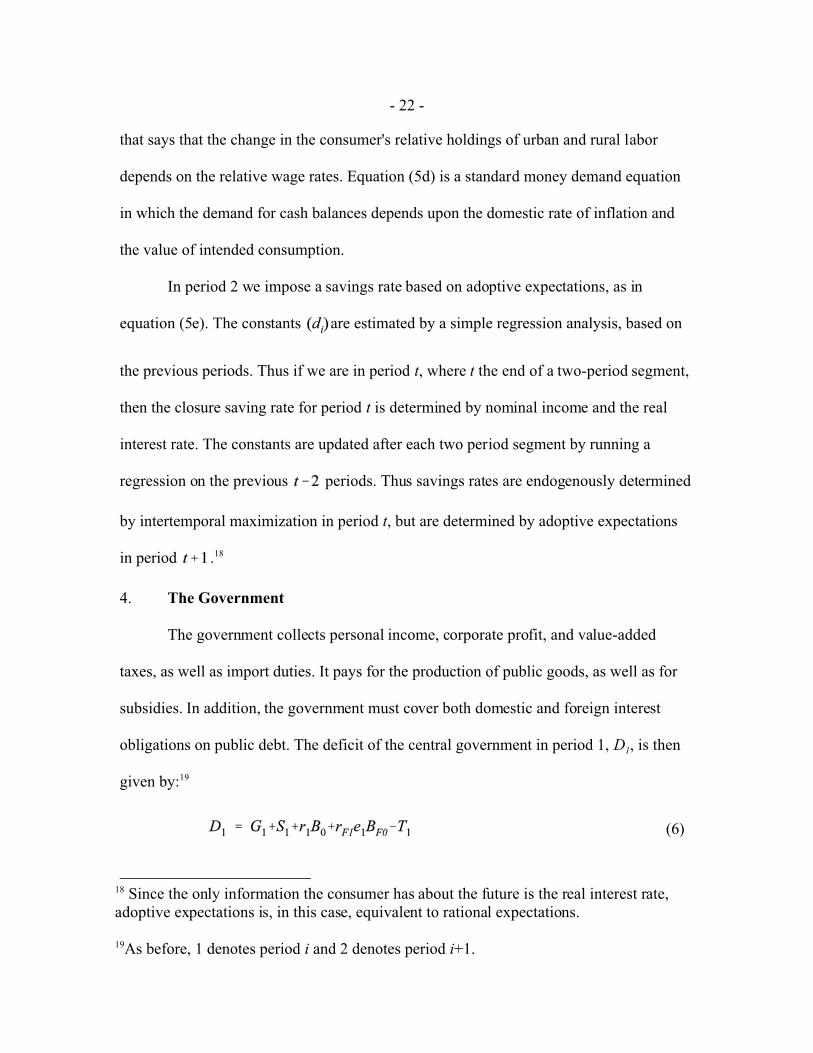
obligations on public debt. The deficit of the central government in period 1, D1, is then

given by:19

- 23 -

(7)

where S1 represents subsidies given in period 1, G1 is spending on goods and services,

while the next two terms reflect domestic and foreign interest obligations of the

government, based on its initial stocks of debt. T1 represents tax revenues, which is

partially determined by firms’ entry into the underground economy.

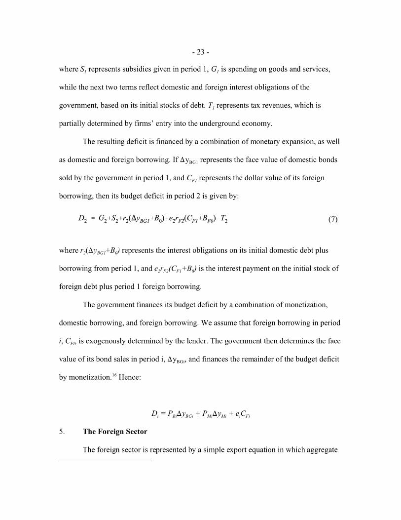
The resulting deficit is financed by a combination of monetary expansion, as well

as domestic and foreign borrowing. If )yBG1 represents the face value of domestic bonds

sold by the government in period 1, and CF1 represents the dollar value of its foreign

borrowing, then its budget deficit in period 2 is given by:

where r2()yBG1+B0) represents the interest obligations on its initial domestic debt plus

borrowing from period 1, and e2rF2(CF1+B0) is the interest payment on the initial stock of

foreign debt plus period 1 foreign borrowing.

The government finances its budget deficit by a combination of monetization,

domestic borrowing, and foreign borrowing. We assume that foreign borrowing in period

i, CFi, is exogenously determined by the lender. The government then determines the face

value of its bond sales in period i, )yBGi, and finances the remainder of the budget deficit

by monetization.16 Hence:

Di = PBi)yBGi + PMi)yMi + eiCFi

5. The Foreign Sector

The foreign sector is represented by a simple export equation in which aggregate

- 24 -

17 We have used various parameters derived from Iqbal (1994, 1998) as well as Feltensteinand Shah (1993) in order to implement the functional forms of our model.

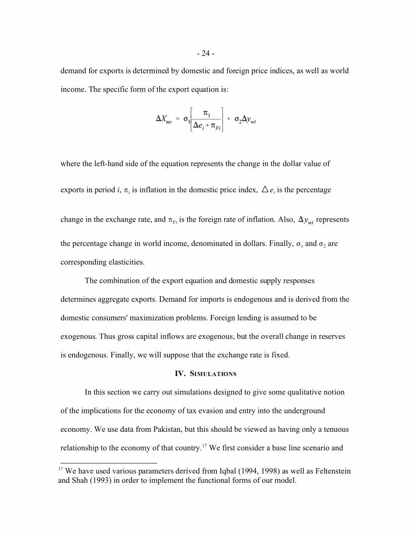
demand for exports is determined by domestic and foreign price indices, as well as world

income. The specific form of the export equation is:

where the left-hand side of the equation represents the change in the dollar value of

exports in period i, B i is inflation in the domestic price index, Îei is the percentage

change in the exchange rate, and BFi is the foreign rate of inflation. Also, represents

the percentage change in world income, denominated in dollars. Finally, F1 and F2 are

corresponding elasticities.

The combination of the export equation and domestic supply responses

determines aggregate exports. Demand for imports is endogenous and is derived from the

domestic consumers' maximization problems. Foreign lending is assumed to be

exogenous. Thus gross capital inflows are exogenous, but the overall change in reserves

is endogenous. Finally, we will suppose that the exchange rate is fixed.

IV. SIMULATIONS

In this section we carry out simulations designed to give some qualitative notion

of the implications for the economy of tax evasion and entry into the underground

economy. We use data from Pakistan, but this should be viewed as having only a tenuous

relationship to the economy of that country.17 We first consider a base line scenario and

- 25 -

18 In practice, we take 1993 as the base year. By this we mean that initial allocations of factorsand financial assets are given by stocks at the end of 1992. We have data for fiscal and otherpolicy parameters for the next 8 years, that is, through 2000.

then carry out certain counterfactual exercises designed to analyze the effects of

alternative tax policies in reducing the size of the underground economy.

In order to use our model for counterfactual simulations, we first generate an

equilibrium using benchmark policy parameters. We run the macroeconomic model

forward for eight years,18 giving tax rates and public expenditures their estimated values.

In particular, we assume an effective corporate tax rate of 13 percent. We also suppose

that the central bank maintains a fixed exchange rate, with the rate being fixed at the

level of the first year.

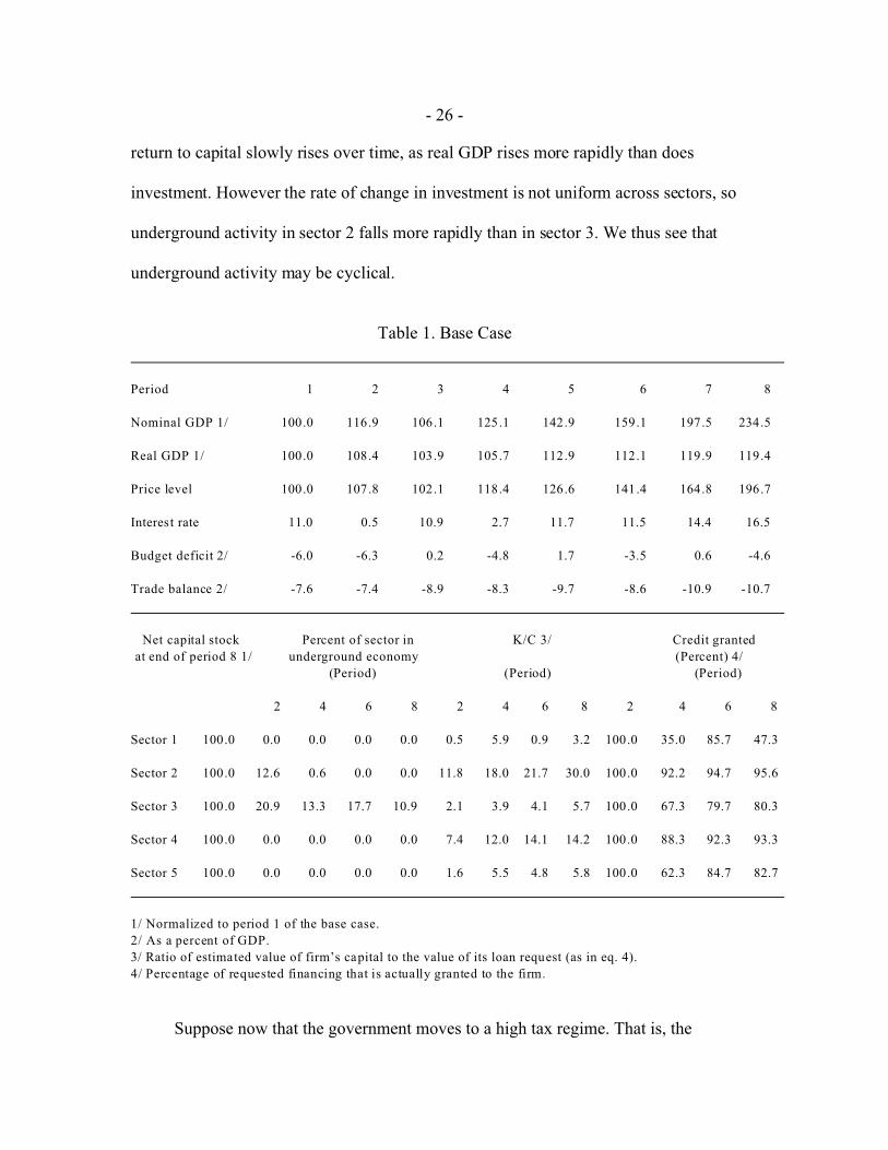
Table 1 shows the results of the benchmark simulation. It may be worth making a

few remarks concerning the simulated values. We do not wish to make comparisons with

actual historical data, given the illustrative nature of this example. First notice that our

model generates moderate rates of growth in real GDP for the first seven periods, after

which real growth stagnates. This is primarily the result of the fixed nominal exchange

rate, which becomes progressively overvalued. The budget deficit improves, and then

fluctuates as activity in the underground economy declines. At the same time, however,

credit rationing fluctuates.. Similarly, interest rates decline and then begin to rise.

It is useful to observe the change in participation of the different sectors in the

underground economy. We see that sectors 2 and 3 both have a share of their activity in

the underground economy during the initial periods. Over time, their underground

activity falls as a share of their total output. The reason for this decline is that the rate of

- 26 -

return to capital slowly rises over time, as real GDP rises more rapidly than does

investment. However the rate of change in investment is not uniform across sectors, so

underground activity in sector 2 falls more rapidly than in sector 3. We thus see that

underground activity may be cyclical.

Table 1. Base Case

Period 1 2 3 4 5 6 7 8

Nominal GDP 1/ 100.0 116.9 106.1 125.1 142.9 159.1 197.5 234.5

Real GDP 1/ 100.0 108.4 103.9 105.7 112.9 112.1 119.9 119.4

Price level 100.0 107.8 102.1 118.4 126.6 141.4 164.8 196.7

Interest rate 11.0 0.5 10.9 2.7 11.7 11.5 14.4 16.5

Budget deficit 2/ -6.0 -6.3 0.2 -4.8 1.7 -3.5 0.6 -4.6

Trade balance 2/ -7.6 -7.4 -8.9 -8.3 -9.7 -8.6 -10.9 -10.7

Net capital stock Percent of sector in K/C 3/ Credit granted

at end of period 8 1/ underground economy (Percent) 4/

(Period) (Period) (Period)

2 4 6 8 2 4 6 8 2 4 6 8

Sector 1 100.0 0.0 0.0 0.0 0.0 0.5 5.9 0.9 3.2 100.0 35.0 85.7 47.3

Sector 2 100.0 12.6 0.6 0.0 0.0 11.8 18.0 21.7 30.0 100.0 92.2 94.7 95.6

Sector 3 100.0 20.9 13.3 17.7 10.9 2.1 3.9 4.1 5.7 100.0 67.3 79.7 80.3

Sector 4 100.0 0.0 0.0 0.0 0.0 7.4 12.0 14.1 14.2 100.0 88.3 92.3 93.3

Sector 5 100.0 0.0 0.0 0.0 0.0 1.6 5.5 4.8 5.8 100.0 62.3 84.7 82.7

1/ Normalized to period 1 of the base case.

2/ As a percent of GDP.

3/ Ratio of estimated value of firm’s capital to the value of its loan request (as in eq. 4).

4/ Percentage of requested financing that is actually granted to the firm.

Suppose now that the government moves to a high tax regime. That is, the

- 27 -

19 If we compare credit granted in Tables 1 and 2, we see that the percentage of requestedloans that is actually granted generally declines in Table 2.

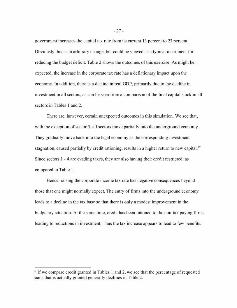
government increases the capital tax rate from its current 13 percent to 23 percent.

Obviously this is an arbitrary change, but could be viewed as a typical instrument for

reducing the budget deficit. Table 2 shows the outcomes of this exercise. As might be

expected, the increase in the corporate tax rate has a deflationary impact upon the

economy. In addition, there is a decline in real GDP, primarily due to the decline in

investment in all sectors, as can be seen from a comparison of the final capital stock in all

sectors in Tables 1 and 2.

There are, however, certain unexpected outcomes in this simulation. We see that,

with the exception of sector 5, all sectors move partially into the underground economy.

They gradually move back into the legal economy as the corresponding investment

stagnation, caused partially by credit rationing, results in a higher return to new capital.19

Since sectors 1 - 4 are evading taxes, they are also having their credit restricted, as

compared to Table 1.

Hence, raising the corporate income tax rate has negative consequences beyond

those that one might normally expect. The entry of firms into the underground economy

leads to a decline in the tax base so that there is only a modest improvement in the

budgetary situation. At the same time, credit has been rationed to the non-tax paying firms,

leading to reductions in investment. Thus the tax increase appears to lead to few benefits.

- 28 -

Table 2. Capital Tax Rate Increase

Period 1 2 3 4 5 6 7 8

Nominal GDP 1/ 100.5 117.0 105.5 123.8 128.2 144.2 172.2 200.9

Real GDP 1/ 100.5 108.7 103.9 105.1 110.7 110.8 117.4 116.8

Price level 99.9 107.6 101.5 117.8 115.8 130.2 146.7 172.1

Interest rate 11.0 0.4 8.8 -0.4 13.5 12.2 13.4 14.1

Budget deficit 2/ -5.4 -6.2 0.9 -4.4 2.3 -3.6 2.0 -3.8

Trade balance 2/ -7.8 -7.4 -9.0 -8.4 -8.9 -7.9 -10.0 -9.7

Net capital stock Percent of sector in K/C 3/ Credit granted



2 4 6 8 2 4 6 8 2 4 6 8

Sector 1 98.2 64.4 58.9 56.4 23.3 0.2 12.8 0.4 9.3 100.0 18.3 92.7 26.3

Sector 2 98.6 79.1 77.8 75.4 71.2 5.6 10.2 10.7 13.6 100.0 85.4 91.1 91.4

Sector 3 91.2 85.3 85.7 87.4 80.0 0.8 3.4 1.6 3.1 100.0 39.6 77.0 62.0

Sector 4 96.6 61.4 63.1 63.0 48.0 3.2 6.4 6.3 8.4 100.0 76.3 86.7 86.3

Sector 5 97.9 0.0 0.0 0.0 0.0 1.4 5.0 4.3 5.2 100.0 58.7 83.3 81.3





Suppose now that the government decides to move in the opposite direction. That is,

it lowers taxes. Such a policy might be carried out as an attempt to create something like a

Laffer effect that increases tax revenues by increasing economic activity in response to

lower taxes, while reducing the attractiveness of entry into the underground economy. As

an extreme example, we will reduce the corporate income tax rate to 3 percent, from the

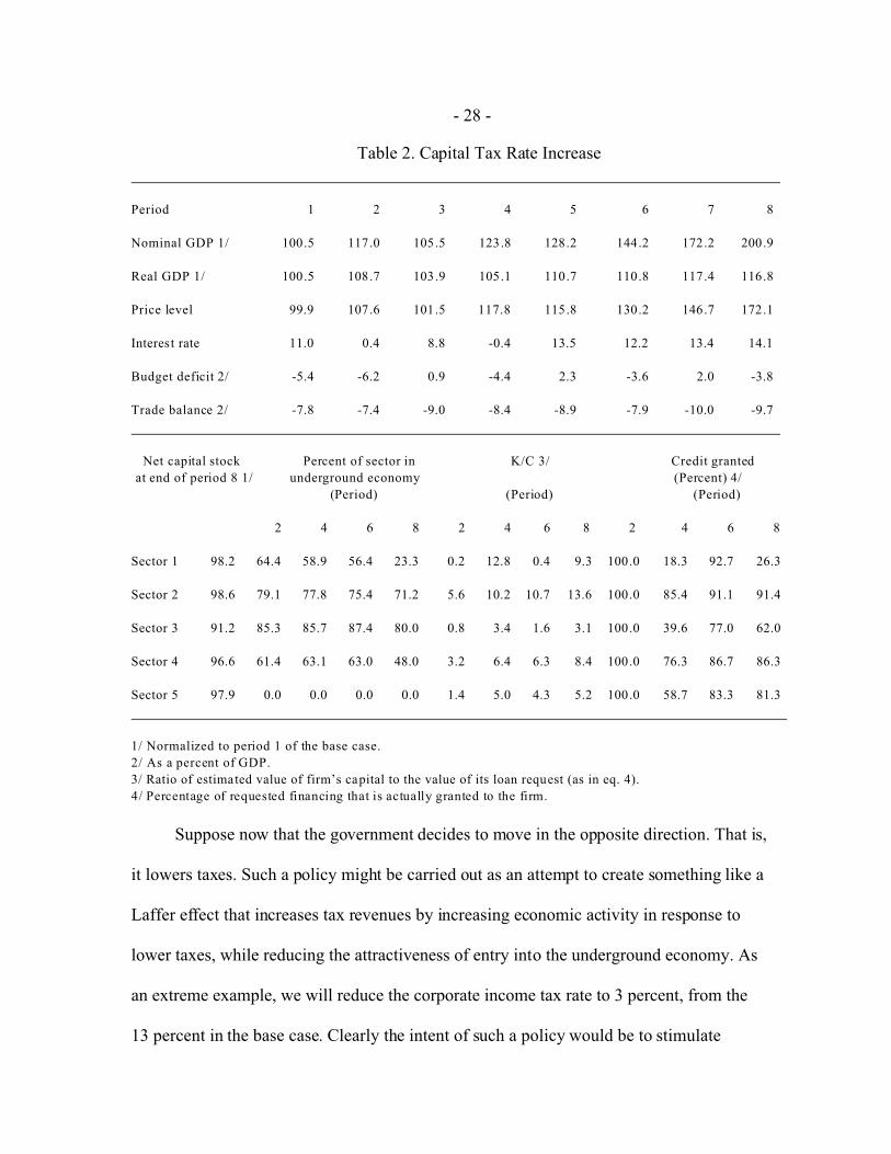
13 percent in the base case. Clearly the intent of such a policy would be to stimulate

- 29 -

growth by increasing both investment and consumption. At the same time, lower tax rates

would presumably discourage underground activity and therefore enhance the tax base.

Table 3 gives the outcomes of the low tax case

Table 3. Capital Tax Rate Decrease

Period 1 2 3 4 5 6 7 8

Nominal GDP 1/ 103.7 117.2 120.5 130.4 184.1 219.5 248.2 306.9

Real GDP 1/ 101.4 108.0 107.1 106.7 117.7 118.2 123.4 122.5

Price level 102.2 108.6 112.5 122.3 156.4 185.7 201.1 250.5

Interest rate 11.2 2.8 11.7 11.1 15.2 17.6 26.5 38.0

Budget deficit 2/ -7.4 -8.2 -2.2 -7.6 -1.7 -5.9 -5.2 -11.3

Trade balance 2/ -8.0 -7.3 -9.5 -7.9 -10.8 -10.8 -12.0 -12.4

Net capital stock Percent of section in K/C 3/ Credit granted



2 4 6 8 2 4 6 8 2 4 6 8

Sector 1 104.3 0.0 0.0 0.0 0.0 1,1 5.4 1.6 3.7 100.0 51.7 86.3 61.7

Sector 2 100.0 0.0 0.0 0.0 0.0 38.7 51.3 78.6 90.9 100.0 97.5 98.1 98.7

Sector 3 108.5 0.0 0.0 0.0 0.0 6.1 11.2 10.7 14.3 100.0 85.7 91.7 91.3

Sector 4 102.7 0.0 0.0 0.0 0.0 14.0 22.7 22.7 30.2 100.0 93.3 95.7 95.8

Sector 5 104.8 0.0 0.0 0.0 0.0 3.0 8.3 7.2 10.9 100.0 75.3 89.3 87.3





Again, there are some unexpected changes, as compared to the base case. We see

that, although there is no underground activity, the rate of capital formation has increased

- 30 -

significantly in only one sector. This is largely due to the fact that the budget deficit has

more than doubled, leading to crowding out of private investment by public borrowing.

There is a corresponding rapid rise in the interest rate, which tends to outweigh the impact

on investment of the tax decrease. Indeed, the rate of investment has slowed significantly

by the final period. At the same time, the average annual inflation rate rises from

10.1 percent to 13.7 percent. Also, the trade balance deteriorates as increases in the

monetary base combine with the assumed fixed exchange rate regime. As might be

expected, the share of credit requested that is actually granted has risen, as compared to

Table 1. As firm’s fully pay their taxes, the corresponding bank estimate of their net worth

rises, leading to lower credit restrictions.

Hence, we may conclude that the low tax regime is not sustainable over time, due to

increases in the budget and trade deficits, even though it eliminates underground economic

activity and reduces credit rationing. Accordingly, we may conclude that it might well be

possible to have tax rates that induce some underground behavior, yet are nonetheless

optimal for the overall economy. At the same time, moderate tax increases can lead to

entry into the underground economy and credit rationing that have a significant

recessionary impact on the economy.

V. SUMMARY AND CONCLUSION

We use a dynamic general equilibrium structure in which optimizing firms compare

the rate of return on investment with the corporate tax rate to analyze the determinants and

effects of an underground economy for public finances and the macroeconomy. If the tax

rate is higher than the return to investment, the firm moves underground, that is, it engages

- 31 -

in tax evasion. At the same time, a firm that evades taxes is subject to credit rationing by

banks.

We carry out a series of simulations of the model, based on stylized data from

Pakistan. Since we have not estimated any parameters, our results should be viewed as

having only a tenuous relationship to reality. A benchmark simulation, using actual tax

rates, shows that entry into the underground economy can have a cyclical nature, as the rate

of return on investment changes. A second simulation raises the corporate tax rate, as a

possible anti-budget deficit policy. This turn out to be counterproductive with a large

amount of production fleeing to the underground economy, thereby lowering the tax base

and actually increasing the deficit. Aggregate investment in the economy and, hence,

growth, is lowered due to greater credit rationing by the banking system. A third simulation

reduces the corporate tax rate, with the intent of creating Laffer curve effects. This policy

does, indeed, eliminate underground activity, but at the cost of high rates of inflation,

increased budget deficit, and a loss of foreign reserves. Hence this scenario is not

sustainable in the long run.

We may thus conclude that it is possible that, in the absence of any flexibility to

adjust expenditures, an economy may have to accept some underground activity, that is, tax

evasion as part of an otherwise acceptable tax program. We have not considered the

possibility of a government enforcement technology that might reduce the incidence of tax

evasion. Also, we have not looked at the impact of productive government spending on

infrastructure and property rights protection in reducing the underground economy. These

may represent directions for future research

- 32 -

REFERENCES

Ahmed, M. A., and Masood, Q., 1995, “Estimation of the Black Economy of Pakistanthrough the Monetary Approach,” The Pakistan Development Review, Vol. 34,pp. 791-807.

Ball, S., and A. Feltenstein, 2001, “Bank Failures and Fiscal Austerity: Policy Prescriptionsfor a Developing Country,” Journal of Public Economics, Vol. 82 (November),pp. 247-70.

Blejer, M., E. Feldman, and A. Feltenstein, 2002, “Exogenous Shocks, Contagion, andBank Soundness: A Macroeconomic Framework,” Journal of International Money and Finance, Vol. 21, pp. 33-52.

Braun, J., and Loayza, N., 1993, “Taxation, Public Services, and the Informal Sector in aModel of Endogenous Growth” (unpublished, Harvard University).

Burgess, R., and N. Stern, 1993, “Taxation and Development,” Journal of Economic Literature, Vol. 31 (June), pp. 762-830.

De Soto, H., 1989, The Other Path (New York: Harper and Row).

Dessy, S., and Stéphane P., 2003, “ Taxes, Inequality and the Sizeof the Informal Sector,” Journal of Development Economics Vol. 70(1), 225-233

Djankov, S., La Porta, R., Lopez de Silanes, F., and Shliefer, A., 2002, “The Regulation of Entry,” Quarterly Journal of Economics Vol. 117, 1-37.

Feltenstein, A., and A. Shah, 1993, “General Equilibrium Effects of Taxation on Investment in a Developing Country: The Case of Pakistan,” Public Finance, Vol. 48, No. 3, pp. 366-86.

Friedman, E., Johnson, S., Kaufmann, D., and Zoido-Lobaton, P., “Dodging the grabbing hand: the determinants of unofficial activity in 69 countries,” Journal of Public Economics, Vol. 76, pp. 459-493.

Huq, M., and M. Sultan, 1991, “Informality in Development: The Poor as Entrepreneurs inBangladesh,” in The Silent Revolution, L. Chickering et al. eds. (San Francisco:International Center for Economic Growth Publication).

Johnson, S., Kaufmann, D., and Shleifer, A., 1997 “The Unofficial Economy inTransition,” Brookings Paper on Economic Activity, Brookings Institute, pp. 159-239.

- 33 -

Johnson, S., Kaufmann, D., and Zoido-Lobaton, P., 1998, “Corruption, Public Finance andthe Unofficial Economy,” ECLAC conference (draft).

Johnson, S., Kaufmann, D., McMillan, J., and Woodruff, C., 2000, “Why do Firms Hide?”, Journal of Public Economics, Vol. 76, pp. 495-520.

Kiyotaki, N., and J. Moore, 1997, “Credit Cycles,” Journal of Political Economy, Vol.105No. 2.

Kydland, F., and E. Prescott, 1977, “Rules Rather than Discretion: The Inconsistency ofOptimal Plans,” Journal of Political Economy Vol. 85, No. 3, June, pp. 473-91.

McMillan J., and Woodruff, C.,1999, “Interfirm Relationships and Informal Credit in Vietnam,” Quarterly Journal of Economics, Vol. 114, pp. 1285-1320.

Sarte, P., 2000, “Informality and Rent-Seeking Bureaucracies in a Model of Long-RunGrowth,” Journal of Monetary Economics, Vol. 46, pp. 173-97.

Schneider, F., and Enste, D., 2000, “Shadow Economies: Sizes, Causes and Consequences,”Journal of Economic Perspectives, Vol. 38, pp. 77-114.

Shleifer, A., and Vishny, R., 1993, “Corruption,” Quarterly Journal of Economics, pp. 599-618.

Shliefer, A., 1997, “Schumpter Lecture: Government in Transition,” European EconomicReview.

Straub, S., 2003, “Informal Sector: The Credit Market Channel,” Department of EconomicsWorking Paper, University of Edinburgh.

Strotz, R., 1956, “Myopia and Inconsistency in Dynamic Utility Maximization,” Review ofEconomic Studies, Vol. 23 (3), No. 62, pp.165-80.

- 34 -

- 35 -