An Analysis of FormationDisruption in Soccer
The Harvard community has made thisarticle openly available. Please share howthis access benefits you. Your story matters
Citation Ma, Jonathan. 2020. An Analysis of Formation Disruption in Soccer.Bachelor's thesis, Harvard College.
Citable link https://nrs.harvard.edu/URN-3:HUL.INSTREPOS:37364766
Terms of Use This article was downloaded from Harvard University’s DASHrepository, and is made available under the terms and conditionsapplicable to Other Posted Material, as set forth at http://nrs.harvard.edu/urn-3:HUL.InstRepos:dash.current.terms-of-use#LAA

An Analysis of Formation Disruption in Soccer
Jonathan MaDepartment of Applied Mathematics
Harvard University
April 3, 2020

Contents
1 Introduction 41.1 A (brief) history of the modern defensive press . . . . . . . . . . . . . . . . . 41.2 Formation Transitions in the Gegenpress . . . . . . . . . . . . . . . . . . . . 51.3 Thesis Outline . . . . . . . . . . . . . . . . . . . . . . . . . . . . . . . . . . . 7
2 A (Brief) Survey of Data Science in Football 82.1 Beginnings: The Expected-Goals Model . . . . . . . . . . . . . . . . . . . . . 82.2 The Historical Importance of Space . . . . . . . . . . . . . . . . . . . . . . . 92.3 Models to Understand Spatial Control . . . . . . . . . . . . . . . . . . . . . 9
2.3.1 A Possession Value Framework through Deep Learning . . . . . . . . 92.3.2 The Spearman Pitch Control Model . . . . . . . . . . . . . . . . . . . 122.3.3 Disruption Surfaces . . . . . . . . . . . . . . . . . . . . . . . . . . . . 13
2.4 Interlude: Formations to Control Space . . . . . . . . . . . . . . . . . . . . . 142.5 Modeling Spatial Disruption . . . . . . . . . . . . . . . . . . . . . . . . . . . 15
2.5.1 The Kempe Defensive Disruptiveness Model . . . . . . . . . . . . . . 152.5.2 The Shaw-Glickman Model . . . . . . . . . . . . . . . . . . . . . . . 162.5.3 The Model of Bialkowski et al. . . . . . . . . . . . . . . . . . . . . . . 172.5.4 Spatiotemporal Trajectory Clustering of Transitions . . . . . . . . . . 172.5.5 Data-Driven Ghosting . . . . . . . . . . . . . . . . . . . . . . . . . . 20
2.6 Summary . . . . . . . . . . . . . . . . . . . . . . . . . . . . . . . . . . . . . 20
3 The Bialkowski et al. Model 213.1 Theoretical Overview . . . . . . . . . . . . . . . . . . . . . . . . . . . . . . . 21
3.1.1 Input Data . . . . . . . . . . . . . . . . . . . . . . . . . . . . . . . . 223.1.2 Objective Function . . . . . . . . . . . . . . . . . . . . . . . . . . . . 22
3.2 An Expectation-Maximization-like Algorithm . . . . . . . . . . . . . . . . . 233.2.1 Analysis of Formations . . . . . . . . . . . . . . . . . . . . . . . . . . 243.2.2 Important Features and Advantages . . . . . . . . . . . . . . . . . . . 253.2.3 Areas to Build Upon . . . . . . . . . . . . . . . . . . . . . . . . . . . 25
4 Implementing the Bialkowski et al. Model 274.1 Data . . . . . . . . . . . . . . . . . . . . . . . . . . . . . . . . . . . . . . . . 274.2 Our Implementation Steps . . . . . . . . . . . . . . . . . . . . . . . . . . . . 28
4.2.1 Step 0: Possession Generation . . . . . . . . . . . . . . . . . . . . . . 284.2.2 Step 1. Selecting Possessions for Role Classification . . . . . . . . . . 28
1

4.2.3 Steps 2-3. Window Generation . . . . . . . . . . . . . . . . . . . . . 304.2.4 EM Algorithm . . . . . . . . . . . . . . . . . . . . . . . . . . . . . . . 324.2.5 Role Labeling . . . . . . . . . . . . . . . . . . . . . . . . . . . . . . . 33
4.3 Role Classification Results . . . . . . . . . . . . . . . . . . . . . . . . . . . . 34
5 Bootstrap Analysis of Formation Changes 355.1 Overview and Comparison with B2014 Model . . . . . . . . . . . . . . . . . 355.2 Data for Bootstrapping: Club X . . . . . . . . . . . . . . . . . . . . . . . . . 365.3 The Circular Block Bootstrap . . . . . . . . . . . . . . . . . . . . . . . . . . 37
5.3.1 Our implementation . . . . . . . . . . . . . . . . . . . . . . . . . . . 375.4 Bootstrapped Distribution of Total 2-Wasserstein Metric . . . . . . . . . . . 395.5 Proof of Concept: Significance Evaluation of Known Formation Changes . . 405.6 Results . . . . . . . . . . . . . . . . . . . . . . . . . . . . . . . . . . . . . . . 415.7 Discussion and Summary of Bootstrapping Results . . . . . . . . . . . . . . 42
5.7.1 Interpreting the Distribution of 2-Wasserstein Distances of KnownFormation Changes . . . . . . . . . . . . . . . . . . . . . . . . . . . . 43
5.7.2 Implications and Future Work . . . . . . . . . . . . . . . . . . . . . . 43
6 Disruption 456.1 Chi-squared statistic as disruption metric . . . . . . . . . . . . . . . . . . . . 456.2 Window Selection . . . . . . . . . . . . . . . . . . . . . . . . . . . . . . . . . 466.3 Chi-Squared Statistic Computation . . . . . . . . . . . . . . . . . . . . . . . 476.4 Comparison with Other Models of Defensive Disruption . . . . . . . . . . . . 486.5 Disruption Results . . . . . . . . . . . . . . . . . . . . . . . . . . . . . . . . 486.6 Other Disruption Statistics: Recovery Time . . . . . . . . . . . . . . . . . . 50
6.6.1 Computing Recovery time . . . . . . . . . . . . . . . . . . . . . . . . 506.6.2 Segmentation of Turnovers by Location . . . . . . . . . . . . . . . . . 526.6.3 Recovery Time Results . . . . . . . . . . . . . . . . . . . . . . . . . . 53
6.7 At-Fault Statistics . . . . . . . . . . . . . . . . . . . . . . . . . . . . . . . . 556.7.1 Design . . . . . . . . . . . . . . . . . . . . . . . . . . . . . . . . . . . 556.7.2 Implementation Plan . . . . . . . . . . . . . . . . . . . . . . . . . . . 56
7 Conclusion 577.1 Concluding Remarks . . . . . . . . . . . . . . . . . . . . . . . . . . . . . . . 577.2 Acknowledgements . . . . . . . . . . . . . . . . . . . . . . . . . . . . . . . . 58
2

Abstract
Modern soccer tactics are largely designed with the objective of maintaining control of spaceon the pitch. In order to maximize their command of space, a team will deploy their playersin a specific arrangement known as a formation. However, certain situations may cause adefending team to temporarily shift away from their defensive formation, and in this disruptedstate they may be more vulnerable to attack. In this paper, we use tracking and event datafrom matches in an elite European soccer league to develop an analysis of formation changes aswell as of defensive disruption. We begin by creating our own implementation of a techniquedeveloped by Bialkowski et al. (2014) to discover formations from tracking data. Based onthe results from this implementation, we develop a new method of identifying statisticallysignificant changes in a team’s formation using comparisons to a bootstrapped distributionof a 2-Wasserstein distance metric. In addition, we also compute a chi-squared statistic thatquantifies the defensive disruption of a team at any time in a match, and we characterizepossible implications of trends in this statistic. Our work in this paper can serve as a first steptowards a better understanding of when formations change as well as when teams becomedefensively disrupted.
3

Chapter 1
Introduction
Gegenpressing lets you win back the ball nearer to the goal. It’s only one pass awayfrom a really good opportunity. No playmaker in the world can be as good as a goodgegenpressing situation, and that’s why it’s so important.
Jurgen Klopp, Liverpool F. C. manager [9]
1.1 A (brief) history of the modern defensive press
In the past ten years, perhaps no single defensive philosophy has shaped the evolution of
modern football1 more than the concept of the defensive press—in other words, actively
attempting to win back the ball after losing it near the opponent’s goal. Pep Guardiola’s
Barcelona, for example, were recognized for their ferocious pressing tactics [16]. Guardiola
recognized that after forcing a turnover, opponents would be vulnerable to being themselves
dispossessed, as they would still be organizing themselves into position and would consequently
be more prone to mistakes. Consequently, Guardiola implemented his famous ”Six-Second
Rule”: immediately after losing possession, his Barcelona teams would cut off passing lanes
for six seconds in an attempt to win the ball back, before falling back to a conventional
defensive formation [16].
The success of Guardiola’s pressing philosophy at Barcelona and elsewhere was quickly
noticed, and before long many of the world’s most prominent managers began incorporating
the press into their own defensive strategies [17]. Perhaps the best-known of these managers
1We will use “football” and “soccer” interchangeably throughout this paper.
4

is current Liverpool manager Jurgen Klopp, who in his previous appointment at Borussia
Dortmund developed the now well-known concept of gegenpressing (literally, ”counter-
pressing”). In essence, the gegenpress took the defensive press that Guardiola had made
famous and added an attacking focus. Proponents of the gegenpress like Klopp believe that
when an opposing team forces a turnover, they begin shifting from a defensive formation to
an offensive one. If the gegenpressing team can then win the ball back at such a time, the
opposing team is then extremely vulnerable to counterattack, because they have moved to
attack and are therefore no longer in their optimal defensive formation [9].
Klopp’s Dortmund vindicated their manager’s belief in the gegenpress with back-to-back
Bundesliga titles, an impressive achievement in a league historically dominated by powerhouse
club Bayern Munich [9]. Today, the pressing concepts developed by Klopp, Guardiola and
others continues to be arguably the most important influence on footballing tactics.
1.2 Formation Transitions in the Gegenpress
Proponents of pressing schemes such as those employed by Guardiola and Klopp often cite two
principal conditions under which the immense amounts of energy expended in chasing down
the ball under such systems are justified [18]. As it turns out, whether these conditions hold
depends on the susceptibility of the opponent or the pressing team to defensive disruption. In
other words, a team usually has a defensive formation (we will define what a formation is in
Chapter 2) which dictates where players should be; whether pressing is worthwhile depends
largely on whether both teams’ players tend to drift away from those positions—in other
words, their tendency towards defensive disruption. We will explore each of these conditions
below.
Firstly, as Klopp states, turnovers resulting from a press often lead to better attacking
chances. Why is this the case? Although pressing ”lets you win back the ball nearer to the
goal” and therefore create a better chance, it is well-known in football that merely being close
5

to the opponent’s goal does not mean that scoring is easy. For example, current Tottenham
manager Jose Mourinho famously found great success earlier in his career by “parking the
bus”–allowing his opponent to advance the ball close to his goal, but keeping all of his players
in a tight defensive formation to defeat any attempt at scoring. Instead, Klopp and others
believe that what makes pressing beneficial to a team’s attack is the creation of disruption in
the opponent’s formation. For example, consider this anecdote from Michael Cox’s Zonal
Marking about a match between Arsenal and Klopp’s Dortmund: [9]
In just six seconds Dortmund managed to lose possession, regain possession
[through gegenpressing ] and score, with their three most dangerous attackers
combining on the edge of the box. Three of Arsenal’s defenders had already
started their offensive transition and began pushing up the pitch before suddenly
finding themselves out of position, and Mkhitaryan’s shot was struck from precisely
the position [Arsenal] left-back Kieran Gibbs had been occupying six seconds
beforehand.
As this example demonstrates, it is the positional disruption of the opponent’s defensive
formation (because they were transitioning into an attack), combined with the proximity of
the turnover to the opponent’s goal, that makes the gegenpress such an effective attacking
strategy. Therefore, the quantification of the transition of a team from defensive to offensive
formations after it has forced a turnover is crucial to determining whether that team will
be vulnerable to the gegenpress. If the opposing team tends to rapidly shift from defense to
attack, then a gegenpressing team may be able to create excellent scoring chances if they are
able to force a turnover through the press. This is the first condition under which a press
may be valuable.
The second condition that makes a press worthwhile has to do with the tendency towards
disruption of the pressing team, not its opponent. While we have already discussed the
offensive value of the gegenpress above, the gegenpress is also defensively valuable because it
can prevent situations in which the pressing team is defensively disrupted. After a team loses
6

the ball, it is often defensively out of formation as it scrambles to recover while the opposing
team is counterattacking [18]. Therefore, characterizing the transition of a team from offensive
to defensive formations after it has forced a turnover is crucial towards determining how
valuable a gegenpress would be for that team. For instance, a team is slow to recover its
defensive formation, then it may as well attempt to win the ball back through the press
because if it does not, it will be hopelessly out of position anyway. This is the second condition
under which a press may be worthwhile.
Thus, we see that the defensive and offensive value of a pressing scheme for any given team
are both predicated upon the tendency of the team and its opponent to become defensively
disrupted in the transition between attack and defense.
1.3 Thesis Outline
The above examples demonstrate the importance of analyzing defensive disruption as a way
of understanding the dominant tactical trends of modern football. In this paper, we will
endeavor to conduct such an analysis.
We will begin, in Chapter 2, with an overview of the data science of football, outlining
important developments ranging from the original expected-goals model, to models of pitch
control, to models of spatial disruption. We will describe the role-classification model of
Bialkowski et al. that we based this project on in Chapter 3. Chapter 4 documents our
implementation of that model and the resulting role classifications. Chapter 5 details a new
method we developed of rapidly identifying formation changes based on a bootstrapping
analysis. Chapter 6 discusses our calculation of defensive disruption, as well as an associated
summary statistic. Chapter 7 concludes.
7

Chapter 2
A (Brief) Survey of Data Science in
Football
2.1 Beginnings: The Expected-Goals Model
At this point, having established the historical importance of space as , we must step aside for
a moment and introduce a seminal paradigm in football analytics: the expected-goals (xG)
model. The original expected goals models, such as the one developed by Sam Green in 2012,
were simply attempts to measure the quality of shot opportunities [1]. Essentially, this basic
xG model is constructed with a logistic regression of whether or not the goal was scored on a
number of input variables, including the type of assist (for example, a cross), the distance
to goal, and the visible angle of the goal [2]. After fitting the model on a training set, the
input variables of any given chance could be fed to the model, and the model’s output—the
xG of the chance—would be considered a measure of chance quality. As Spearman notes,
a number of modifications to this basic xG model have subsequently been developed, each
adding different input variables—such as the location-based “dangerosity” of the possession
that led up to the shot opportunity, the player who is taking the shot, and the body part the
shot is taken with—to improve the model [3] [19] [20].
8

2.2 The Historical Importance of Space
While the xG model was an important development in football analytics, the fewer than a
dozen input features of the model may miss much of the contextual information of how the
shot was created. So, how can we better understand how teams arrive at shot opportunities?
The answer lies in the history of football as a game of space. The great Dutch footballer
Johan Cruyff once stated that [9]
When you’ve got possession of the ball, you have to ensure that you have as much
space as possible, and when you lose the ball you must minimize the space your
opponent has. In fact, everything in football is a function of distance.
For Cruyff, space on the pitch was the lifeblood of an offense. This philosophy, which Cruyff
implemented to excellent effect during his managerial career at Ajax and Barcelona, eventually
became the foundation upon which all football clubs developed their strategy [9].
2.3 Models to Understand Spatial Control
Having established the historical importance of space in modern football, we will now turn to
a series of models, each of which attempts to understand a team’s command of the space on
the pitch. Like Green’s xG model, many of these approaches attempt to model the probability
of goalscoring; however, by relying on spatial analysis rather than solely the selected features
of shot attempts (as with Green’s xG model), these models can compute the offensive value
of a possession even if it does not end in a shot.
2.3.1 A Possession Value Framework through Deep Learning
One example of such an model is the work of Fernandez et al., who attempted to use deep
learning to compute a team’s probability of scoring on any possession [5].
9

Technical Overview of the Fernandez et al. Model
While xG focuses on measuring the quality of a chance, Fernandez et al. model the value of
any given possession of a team, regardless of whether it ended in a goalscoring chance. Their
model is centered around the equation
EPV (t) = E[X|Tt] = E[X|A = ρ]P (A = ρ) +E[X|A = ζ]P (A = ζ) +E[X|A = δ]P (A = δ)
where X is the event that a goal is scored, Tt is all spatiotemporal data available by time t,
and t is the time of interest in the match.
Let us unpack this equation to better understand it. Fernandez et al. model a possession
as consisting of three possible actions A: a pass ρ, a shot ζ, or a drive δ. Consequently, the
expected possession value EPV , defined as the expected probability of scoring a goal on that
possession, can be decomposed into the sum of expectations of scoring a goal conditional on
each of these three actions occurring.
Fernandez et al. model many of these components using deep learning. For example, the
action probabilities P (A = ζ), P (A = ρ), and P (A = δ) are ”modeled through a convolutional
neural network on top of pitch control and pitch influence surfaces” [5]. Similarly, the expected
values from driving and passing—E[X|A = δ] and E[X|A = ρ] respectively—are ”learned
from a set of carefully designed deep neural networks” [5].
Comparison with xG, and drawbacks
It is instructive to compare the model of Fernandez et al. with the xG model. Fundamentally,
both models are attempts to quantify a team’s offensive success by modeling the probability of
scoring. In contrast to the xG model, though, Fernandez et al. also model the ability of a team
to control space—in other words, their “pitch control and pitch influence surfaces”—which
allows them to model the probability of scoring even when there is no shot attempt.
However, one of the drawbacks of neural networks is that they are often difficult to
10

interpret, and while the networks trained by Fernandez et al. demonstrate an impressive
ability to quantify the EPV of a pass to a particular zone, it is unclear how these networks
are generating their predictions. [5] Indeed, Fernandez et al. do not specify the precise
input variables of the networks, report specific weights that result from training, or offer
interpretations of how the networks arrive at their predictions [5].
Moreover, as seen in the philosophies of Klopp and Guardiola amongst others, managers
in modern football increasingly place emphasis on forcing turnovers—whether through a
press, a gegenpress, or other means. Therefore, the ability of the model of Fernandez et al.
to detect the loss of EPV through the risk of turnovers is paramount. Indeed, Fernandez et
al. model the expected value of a possession, given that the player passes, as [5]
E[X|A = ρ] = E[X|A = ρ∩Oρ = 1]P (A = ρ∩Oρ = 1)+P (A = ρ∩Oρ = 0)E[X!A = ρ∩Oρ = 0]
where A = ρ is the event that the player attempts a pass, and Oρ is the probability that the
pass is successful (i.e. not a turnover). Again, note that this equation represents an attempt
to model the attacking team’s control of space on the pitch, through variables such as Oρ.
However, it is again unclear how the logistic regression model that estimates the probability
of turnover operates, as Fernandez et al. do not provide its inputs or the weights of the
trained model. Likewise, the workings of the model which Fernandez et al. use to calculate
the expected value in case of turnover, E[X!A = ρ ∩ Oρ = 0], are unclear. For example,
certain teams—such as many in the Bundesliga when Guardiola was managing Bayern—are
well-known to be extraordinarily proficient at executing counterattacks, so at a minimum any
model that attempts to quantify the EPV of a turnover must identify not only whether the
opponent is such a team but also whether the positioning of the players at the moment of a
turnover allows for a high-value counterattack by the opponent [9].
11

2.3.2 The Spearman Pitch Control Model
In contrast to deep-learning based models, William Spearman invented a probabilistic pitch-
control model which is highly interpretable, and which he uses to quantify the expected
probability of scoring from any current state of a match [3]. In order to understand this
model, we must begin with Spearman’s definition of pitch control, which he developed in a
previous paper [4].
Spearman begins by defining the notion of passing success: the receiver of the pass is
defined asthe first player to demonstrate control of the ball (e.g. by dribbling it) after the
pass occurs, and the pass is successful if the receiver and the passer belong to the same team.
Thus, Spearman models the probability of a successful pass to any location as the probability
that the team can control a ball as it arrives at that location, while accounting for factors
such as player positions relative to the pass destination, the flight time of the pass, etc.
With this basic intuition, we can begin to understand Spearman’s potential pitch control
field (PPCF) model. Essentially, the PPCF can be thought of as a function which, given
a particular state of the match (including the current location of the ball), returns the
probability that a team retains control of the ball for a pass to any given new location on the
pitch. In other words, the PPCF can be written as a function PPCFj(t, ~r|s, λj), which gives
the probability that player j can control the ball if it is passed (with the optimal trajectory)
from its location in the current state s to the new location ~r at time t.
Spearman models the evolution of the PPCF using the differential equation [3]
dPPCFj(t, ~r, T |s, λjdT
=
(1−
∑k
PPCFk(t, ~r, T |s, λj)
)fj(t, ~r, T |s)λj
Intuitively, the expression in the parenthesis is the probability that the ball has not already
been controlled by any of the players after time T has passed from the time t that the pass
was launched, and fj(t, ~r, T |s) represents the probability that player j can reach the location
~r within time T given current game state s. λj is the rate of control: Spearman models
12
the process of player j gaining control of the ball as a Poisson process with parameter λj.
Therefore, we can understand the expression on the right hand side as the probability that
nobody has controlled the ball yet at after time T has elapsed following the current time t,
multiplied by the probability that player j can reach and control the ball after time T has
elapsed.
Integrating the elapsed time T from 0 to ∞, the above expression yields the PPCF at
time t for any pass destination ~r.
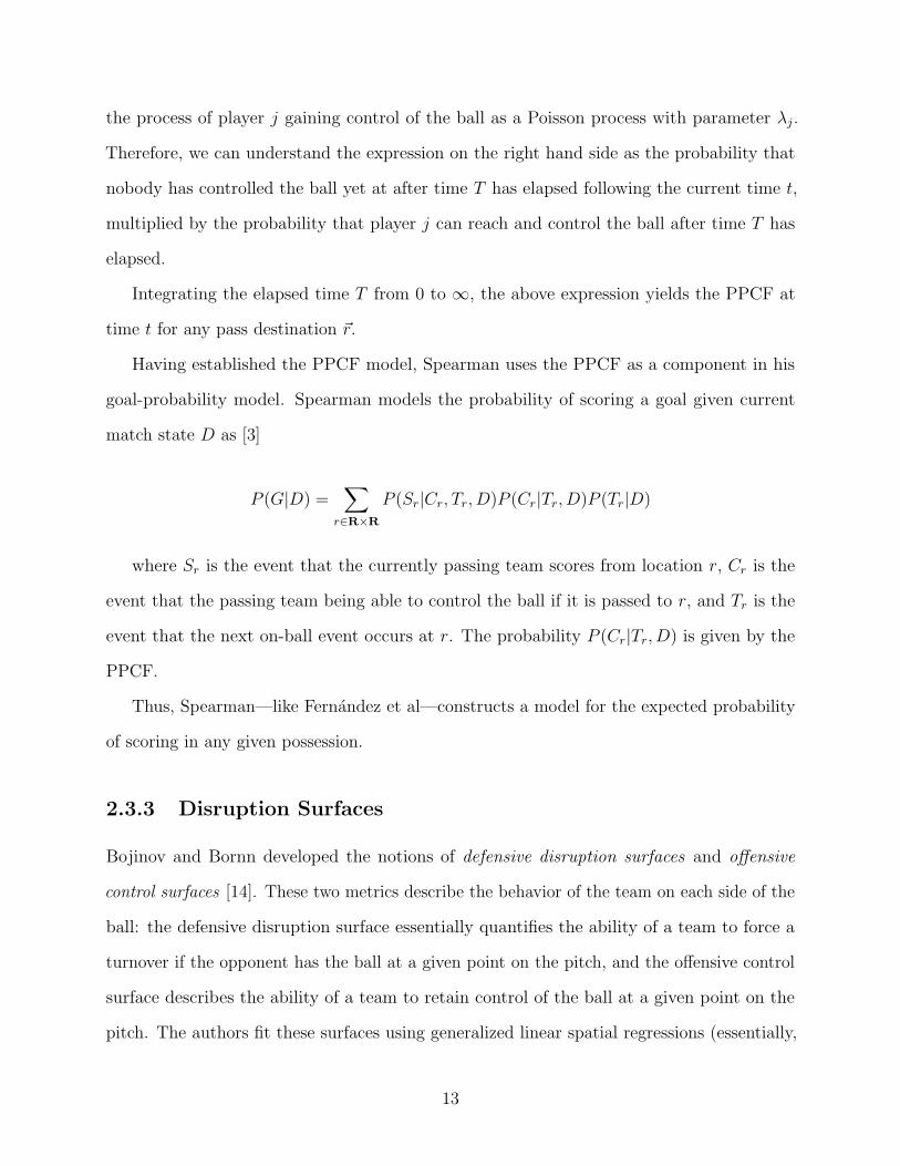
Having established the PPCF model, Spearman uses the PPCF as a component in his
goal-probability model. Spearman models the probability of scoring a goal given current
match state D as [3]
P (G|D) =∑
r∈R×R
P (Sr|Cr, Tr, D)P (Cr|Tr, D)P (Tr|D)
where Sr is the event that the currently passing team scores from location r, Cr is the
event that the passing team being able to control the ball if it is passed to r, and Tr is the
event that the next on-ball event occurs at r. The probability P (Cr|Tr, D) is given by the
PPCF.
Thus, Spearman—like Fernandez et al—constructs a model for the expected probability
of scoring in any given possession.
2.3.3 Disruption Surfaces
Bojinov and Bornn developed the notions of defensive disruption surfaces and offensive
control surfaces [14]. These two metrics describe the behavior of the team on each side of the
ball: the defensive disruption surface essentially quantifies the ability of a team to force a
turnover if the opponent has the ball at a given point on the pitch, and the offensive control
surface describes the ability of a team to retain control of the ball at a given point on the
pitch. The authors fit these surfaces using generalized linear spatial regressions (essentially,
13

regressing a spatially varying response variable—indicating whether a team retains or loses
the ball at each location on the pitch).
Clearly, therefore, the work of Bojinov and Bornn has many commonalities with Spear-
man’s PPCF-based pitch control model. While the authors refer their results as “defensive
disruption,” they are referring to a team’s ability to disrupt an opponent’s possession (the
complement of Spearman’s earlier notion of pitch control, or the ability to retain possession),
rather than the spatial disruption of a team from its desired defensive formation—the focus
of the models discussed in the next section [14].
2.4 Interlude: Formations to Control Space
How does a team systematically maintain control of space on the pitch? The answer lies
in the formation, or the arrangement of a team’s players. (In this paper, we will limit the
notion of the formation to the ten outfield players and exclude the goalkeeper.) For instance,
Cox notes that [9]
The best representation of the Dutch emphasis on space...was in terms of the
formations used by Cruyff’s Barcelona, Van Gaal’s Ajax and the Dutch national
team.
Football formations are usually decomposed into three lines of players: defenders, midfield-
ers, and forwards. (In terms of nomenclature, referring to a formation as a “4-4-2” indicates
that the players are grouped into a line of 4 defenders, a line of 4 midfielders, and a line
of 2 forwards.) The number of players in each line varies between formations, and some
formations may also include players who reside somewhere between two of the lines.
As Cox notes, managers like Cruyff choose formations which they believed would best
allow their teams to control space [9]. However, as illustrated by the Arsenal-Dortmund
example from the Introduction chapter, teams may fall out of formation—in other words,
they may be disrupted—and may be more vulnerable to attack when they do so. In the
14

following section, we will take a look at a series of models which attempt to better understand
this notion of defensive disruption.
2.5 Modeling Spatial Disruption
In the preceding sections, we have described the development of formations as a method
of maximizing a team’s spatial control of the pitch, and we have described models such as
those by Fernandez et al. and Spearman that use pitch control modeling as a step towards
computing expected goal value of possessions. We have also seen in the Introduction that
teams may be vulnerable to attack as they are shifting away from their defensive formation.
In this section, we will introduce several models in the literature which combine these concepts
to analyze the spatial disruption of a team—the deviation of players from the locations on
the pitch where they are supposed to be—and which analyze the implications of spatial
disruption on the offensive value of a possession.
2.5.1 The Kempe Defensive Disruptiveness Model
Kempe et al. attempt to model defensive disruptiveness that results from the attacking
team’s passes [11]. They generate a number of features that describe the changes in defensive
organization of a team in the three seconds following every pass, including the changes in
positions of a team’s center-of-mass and its three defensive lines, as well as the changes in
the area and the spread of the formation. They then used principal component analysis to
create three composite factors out of these features, and report the sum of magnitudes of
those three factors as a defensive disruption score. A subsequent paper by the same authors
improved upon this metric [12].
This approach, like the other models in this section, does model the ability of a pass
to disrupt the spatial organization of a team. In addition, the model of Kempe et al. is
easily interpretable, and the input features (e.g. positions of formational lines) are tactically
15

meaningful. However, a fundamental flaw of this approach is that disruption is not necessarily
induced by a pass. Again, let us revisit the example of the Arsenal-Dortmund game referenced
in the Introduction of this paper. In that example, the Arsenal players were not out of position
defensively because of a well-placed Dortmund pass; they were out of position because they
were expecting to attack but Dortmund gegenpressed and stole the ball from them [9]. The
method of Kempe et al., which predicates the entirety of their analysis on the effects of
the pass, cannot capture or analyze these pressing scenarios that are fundametal to modern
football.
2.5.2 The Shaw-Glickman Model
Shaw and Glickman developed an innovative model to compute the formation of any team
at any moment in a match. The key idea of their approach is to compute the position of
team members relative to their teammates, rather than as an absolute position on the pitch
[15]. Concretely, at any given time the centroid of the formation is set to be the player who
is closest to his teammates (based on the average distance to the third-nearest teammate).
Then, the position of the nearest player A to the centroid is defined relative to the centroid,
the position of the nearest neighbor B to A is defined relative to A, and so on.
Shaw and Glickman demonstrated that this approach successfully extracts formations from
matches, and demonstrate how to identify changes in these formations [15]. Theoretically,
because this model identifies spatial distributions of formations, it could be used as a basis
for understanding how teams deviate from their formations at any given time. However, we
chose to use the model of Bialkowski et al., as will be further detailed and explained in the
following sections, because the method of Bialkowski et al. includes a robust system of role
assignment.
16

2.5.3 The Model of Bialkowski et al.
We eventually decided to use a model developed by Bialkowski et al. (henceforth referred to
as the “B2014 model”) as a basis for this project, so we will not describe it in detail here—an
extensive overview of the model is available in the Methods chapter. For now, it suffices to
summarize the model as a method of role classification, which reassigns a role to each player
at each moment in the match and which produces positional distributions of the roles that
comprise a team’s formation.
2.5.4 Spatiotemporal Trajectory Clustering of Transitions
While the models described in the two preceding sections use pitch control surfaces to analyze
a team’s command of space on the pitch, Hobbs et al. use a different approach to understand
how teams exploit space in transition. Rather than modeling the probability of controlling
the ball at given points on the pitch, Hobbs et al. use tracking data from the English Premier
League to analyze the movements of players and understand how that behavior leads to
scoring [10].
Chalkboarding
To understand the methods of Hobbs et al., we must begin by first understanding the notion
of chalkboarding, which forms the basis of their model. Chalkboarding was developed in an
earlier paper, which considers a team as a collection of roles (each of which can be filled by
any team member) [13]. In the chalkfoarding approach, role distributions are first calculated
using the B2014 model. Next, for any given frame of tracking data, the players are assigned to
roles using the Hungarian algorithm for linear sum assignment. Using this method, therefore,
any play can be encoded as a spatiotemporal trajectory of roles.
17

Creating a Transition Playbook
Hobbs et al. built upon the chalkboarding approach described above to create a “playbook” of
transitions [10]. First, the B2014 model is used to create a universal template formation, and
the players in all training examples (consisting of 10-second interleaved windows from English
Premier League matches) are assigned to roles within that formation by the Hungarian
algorithm. Each training example therefore is now encoded as a set of spatiotemporal
trajectories of roles. Next, the training examples are k-means clustered. For each subcluster,
the template formation is then set to the role trajectories of the parent node (so that the
template formation contains the “average trajectories for each player-assignment in that
cluster”). The preceding steps are then repeated for each cluster with its new template
formation, and the process continues until the clustering tree reaches a maximum depth or a
minimum number of plays in a leaf.
Defensive Disruption Based on the Playbook
Based on this model, Hobbs et al. defined the defensive disruption of a play to be the total
displacement of the players in the play with respect to the formation of the playbook template
closest to that play.
Drawbacks
Despite its many advantages, we believe that the method of Hobbs et al. as described in [10]
has four drawbacks:
Firstly, as with any hierarchical clustering method, there is the problem of misclassification.
Although Hobbs et al. identified 218 different playbook entries, the vast history of soccer has
surely produced more than 218 transition plays and it is impossible to guarantee that this
method will not misclassify a new play that was not in its training set.
Secondly, Hobbs et al. compute the defensive disruption at a particular frame as “the
total displacement or cost associated with moving each player back to his preferred location in
18

the formation”—in other words, the position dictated by his role. However, different roles in
football naturally have different positional variances, even on defense: for example, one would
expect a forward to roam more freely across the pitch and thus have a greater positional
variance than, say, a center-back. Therefore, a team’s coach might consider a forward to
be “within the position dictated by the defensive formation” even if the player is relatively
farther from the centroid of their role distribution. Thus, absolute Euclidean distances are
not a representative metric of disruption.
Thirdly, it appears that Hobbs et al. only compute the total defensive disorder of the
team, rather than the defensive disorder of individual players. Neglecting to assess individual
players’ defensive positioning is problematic: for instance, if even a single center-back is out
of position, their team would be left with a gaping hole in the back line of their defense
directly in front of their goal. However, if the nine other outfield players are very close to
their prescribed formational positions, the total defensive disorder might not be any higher
than usual.
Finally, the model of Hobbs et al. is susceptible to misclassifying a highly defensively
disrupted play as a different play. For example, suppose we are using the Hobbs et al. model
to compute the defensive disorder of a possession in which a given team was instructed by
its coach to follow play A, but a team member drastically fell out of position in a way such
that the team’s spatiotemporal trajectory appeared to resemble play B. Under the Hobbs et
al. model, this play would be classified as an example of play B with low disruption, rather
than an example of play A with high disruption. This type of misclassification is an inherent
consequence of simultaneously classifying a play—by selecting the playbook entry which
minimizes the distance to that play—and reporting that distance metric as the disruption of
the play. Without a predefined notion of what the formation should be at a particular time
in the match, this approach will be susceptible to misclassifications such as the one we have
illustrated, which will lead to erroneously low disruption values.
19

2.5.5 Data-Driven Ghosting
Le et al. used deep imitation learning to develop a model involving ghosting, or predicting
where players should have been at a given time in a match. Their model also begins with role
classification using the B2014 model [21]. Next, Le et al. apply Long Short-Term Memory
neural networks which take these role classifications and other spatial data as input, and
output “ghosted” player positions. The authors also apply numerous imitation learning
methods to prevent errors from compounding over time as they model sequences of player
motion.
By comparing actual player positions with their ghosted positions, Le et al. can compute
the degree of disruption of each player.
2.6 Summary
In this literature review, we have described the development of two principal categories of
models in football analytics. The first is the set of models which, consistent with the focus
on space in modern footballing tactics, attempt to measure a team’s control of space using
metrics such as the PPCF or deep-learning models [3] [5]. The second is the set of models
which, recognizing that teams deploy formations to control space, attempt to analyze how
those formations can become disrupted. In the remainder of this paper, we will discuss how
we constructed our own notion of disruption based on the model of Bialkowski et al., which
we will introduce next.
20
Chapter 3
The Bialkowski et al. Model
In this chapter, we shall introduce the model developed by Bialkowski et al. (henceforth
abbreviated as B2014), which is the model on which this project is based.
The B2014 model was one of the first models to consider a team’s formation in terms of the
positional distribution of roles rather than individual players, which intuitively accounts for
the frequently observed phenomenon of “role switching” in which players exchange the areas
on the pitch they are defending. In the subsequent sections of this chapter, we will summarize
the data used for the model, the objective function, and the steps for implementation of this
model as described by Bialkowski et al. in two papers [6] [7]. Our own implementation of the
B2014 and results will be described in Chapter 4.
3.1 Theoretical Overview
The B2014 model is an intuitive way of obtaining the approximate positional distributions
of each position in a team’s formation across a given time interval. The authors begin by
defining the notion of role as an area of space on the pitch which a player is responsible for
controlling [6]. The roles of the ten outfield players therefore comprise the formation of the
team. Moreover, any role can be occupied by any player, which means that role assignments
may dynamically change over the course of the match.
21

3.1.1 Input Data
The input data of the B2014 model is tracking data—a series of frames, each of which
corresponds to a time in the match. Each frame of tracking data will contain the positions
of all players and the ball, as well as a timestamp. With a frame rate of usually at least 25
frames per second, tracking data can be used to detect accurate trajectories of all players at
all times. This contrasts with event data, which is essentially a series of events (e.g. shot
attempts, red or yellow cards, substitutions, passes, tackles etc.) that occur on or off the ball,
but which contains no information about the players not involved in any given event.
3.1.2 Objective Function
The goal of the model is to assign a role to each player at each unit of time in the match. If
accomplished, the positional distributions of each role could then be calculated (where the
position of a role at a given time is the position of the player assigned to that role at that
time). These positional distributions, which can be thought of as the probability that player
in a given role is in a given position on the pitch, can then be used to visualize the team’s
formation, as seen in Figure 3.1.
So, how are these roles assigned to players? Conceptually, Bialkowski et al. define the
optimal role assignment as the one which maximizes the Kullback-Lieber (KL) divergence
between the resulting role distributions [6]. In other words, with the KL divergence defined
as
KL(P (x)||Q(x)) =
∫P (x) log
(P (x)
Q(x)
)dx
the optimum role assignment in each frame is the one that maximizes the total divergence,
by minimizing the negative total divergence
V = −N∑n=1
KL(Pn(~x)P (~x))
22

Figure 3.1: The convergence of the role classification of Bialkowski et al. as documented in[6]
where N is the total number of players, Pn(~x) is the probability density function of the role
distribution of the n-th player, and P (~x) is the probability density function of the whole team
[6]. Intuitively, the KL divergence quantifies the amount of overlap between two probability
density functions (with identical distributions having zero divergence). Hence, by maximizing
the divergence of role distributions in the formation, this role assignment scheme minimizes
the amount of spatial overlap between roles, ensuring that each role is responsible for a
specific area of the pitch and that as a whole, the team controls as much of the pitch as
possible [6].
3.2 An Expectation-Maximization-like Algorithm
In practice, Bialkowski et al. found that computing role assignments according to this
approach is difficult to efficiently achieve, so they instead approximated these optimal
assignments through an approach similar to the well-known expectation-maximization (EM)
method [6]. They began by assigning each player an arbitrary role throughout the whole
match, and computing the resulting bivariate Gaussian role distributions (with all positions
computed relative to the formation’s center-of-mass, in order to make the analysis invariant
under translation of formations). In each iteration of EM, the authors then calculated the
negative log likelihood that a player i is playing a role j in each frame of the match, based
on the probability distribution of role j, and then used the Hungarian algorithm to reassign
23

Figure 3.2: Formation clusters by Bialkowski et al. as documented in [6]
roles in that frame by maximizing the sum of log likelihoods. Bialkowski et al. repeated
this algorithm for a number of iterations and found that it caused the role distributions
to converge to a formation with low overlap, as seen in Figure 3.1. In that figure, each
ellipse represents the distribution of one of the ten outfield roles, and we can see that the
distributions are almost nonoverlapping [6].
Having computed role classifications, Bialkowski et al. used agglomerative clustering
based on the Earth Mover’s Distance, also known as the Wasserstein Metric, to cluster 1411
formations (sets of 10 role distributions from a match-half) into six clusters, as shown in
Figure 3.2 from their paper [6].
3.2.1 Analysis of Formations
In a subsequent paper, Bialkowski, Lucey, and other co-authors developed further approaches
to identify team formations based on their role classification method. Notably, they adapt
their approach to a five-minute “sliding window,” thereby allowing them to identify the
formation which a team has employed in the past five minutes at any point in the match [7].
In the same paper, the authors also identify formation changes throughout the match using
two distinct approaches. In the first approach, they use k-means clustering to identify each
formation at each point in time with one of four formation clusters obtained from clustering
all formations in the match. (They arbitrarily chose the number of formation clusters.) [7]
In the second approach, they compute of the sum of mean Euclidean distances between the
positions of each role at each time in the match with a standard formation.
24

3.2.2 Important Features and Advantages
We selected the B2014 model as the basis of this project because it contains a number of
extremely advantageous features. Firstly, by reassigning roles to players at each time in a
match, it accounts for phenomena such as recovery runs, in which one player runs to cover
the space of another player who is out of position. In such a situation, the covering player
should be assigned the role he is covering, which the B2014 model can do. Secondly, by
computing formations over an extended period of time, it is less vulnerable to noisy data and
converges to well-shaped formations, as demonstrated by Bialkowski et al. [6]. Finally, the
EM algorithm is computationally efficient, which is important when running it on a dataset
of hundreds of matches.
3.2.3 Areas to Build Upon
Next, we identified a number of areas in the B2014 Model that we would like to build upon
and improve in this paper.
Firstly and perhaps most importantly, the B2014 model does not account for disruption
of formations. For example, Bialkowski et al. use trends in total Euclidean distance from a
template formation to detect whether the team’s formation has changed [7]. However, a team
may fall out of formation temporarily—perhaps as a result of a turnover due to a gegenpress,
as the Arsenal-Dortmund example cited in our Introduction chapter demonstrates—even as
they are attempting to maintain that formation [9]. The B2014 model itself does not account
for or quantify such short-term, temporary disruptions to a team’s formation, even though
Cox’s examples suggest that they may be crucial to understanding how many modern teams
play. As we have noted in Chapter 2, there have been separate attempts to quantify defensive
disruption based upon the B2014 model using approaches such as spatiotemporal tracking,
but these attempts have drawbacks which we have also documented in Chapter 2.
Secondly, Bialkowski et al. also attempt to determine formation changes through ag-
glomerative clustering of formations [6] [7]. However, such a method of detecting formation
25

variation is inherently flawed, because it requires the selection of a distance threshold or a
number of clusters, and it is difficult to determine these hyperparameters ex ante. Moreover,
this clustering method of formation classification does not quantify the statistical significance
of such a classification—an important metric, given that Bialkowski et al found that over 50
percent of the examples belonging to one of the clusters was misidentified as belonging to a
different cluster [6].
Finally, to our knowledge Bialkowski et al. have not provided an open-source implementa-
tion of their approach. (We plan to eventually release both our implementation of the B2014
model and our code for calculating disruption based on that model.)
26

Chapter 4
Implementing the Bialkowski et al.
Model
In this chapter, we describe our implementation of the B2014 model in detail. We begin with
an overview of the data we used as input for the model. Next, we describe our implementation
of the “sliding windows” approach which Bialkowski et al. originally described in [7], as
well as our role-labeling scheme which assigned each player to one of three formational lines.
Finally, we exhibit an example of a role classification distribution which resulted from our
implementation of the B2014 model.
4.1 Data
Our dataset consists of tracking data from 378 matches in an elite European league throughout
the 2018-19 season as well as the 2019-20 season to date. Tracking data contained 2-
dimensional player positions as well as a 3-dimensional ball position in each frame. Each
frame also had a possession indicator as well as a timestamp. The data was collected at a
frequency of 25 frames per second.
For each match, we also had access to event data, which encodes all on-ball events as well
as other events such as formation changes and yellow or red cards. However, as noted earlier,
27

each event datum does not contain any information about the other players not involved in
the event.
4.2 Our Implementation Steps
4.2.1 Step 0: Possession Generation
We used code written by Dr. Laurie Shaw to read the tracking data and then segment
the frame-by-frame tracking data of each match into possessions, defined as a sequence of
frames in which a single team possesses the ball. We then split the formations into two sets:
home-attacking and away-attacking.
From here on, the step numbers will correspond to the steps in Figure 4.1.
4.2.2 Step 1. Selecting Possessions for Role Classification
Only certain possessions are useful for generating role classifications: for example, if a team
has been pushed extremely far back (i.e. close to its own goal), its formation will necessarily
be distorted, as all the players will be defending a small area. In order to avoid such scenarios,
we eliminate all possessions in which the ball is in the defensive quarter of the team possessing
it (in order to eliminate scenarios in which the goalkeeper possesses the ball while the rest
of the team is moving upfield). For the purposes of role classification, we also eliminate
possessions of length less than five seconds, unless the possession begins with a dead ball, as
we assume that on dead balls both teams will have time to move to their desired positions.
Note that these possessions were only eliminated because we believed they would not be
representative of a team’s intended formations—we later reinstated them for the purposes of
the calculation of disruption. I will refer to the remaining possessions after this selection as
“role possessions” and the remaining frames as “role frames.”
28

Figure 4.1: Workflow for our implementation of the B2014 model for role classification.
29

4.2.3 Steps 2-3. Window Generation
First, we separate the possessions by which team is attacking (Step 2), yielding two sets of
possessions which we will henceforth refer to as the away-attacking possession set (AAPS)
and the home-attacking possession set (HAPS).
Of course, a single possession—which typically has a duration on the order of five seconds—
is not enough data to run the B2014 algorithm. Instead, we need to run the algorithm on
a concatenated set of possessions, or a window. These windows are interleaved, analogous
to the “sliding windows” approach of Bialkowski et al., in order to be able to more rapidly
detect formation changes (because by the construction of our approach, we compute a single
formation for each window, so formation changes can only be detected at the transition
between any two windows). Importantly, note that by splitting the possessions into two sets
based on which team is attacking and creating a set of interleaved windows for each, we
have ensured that each team has separate sets of windows in which they are attacking and
defending. For example, all the frames in which the home team are on defense (and, therefore,
the away team is attacking) can be found in the windows generated from the AAPS.
We use two distinct methods to generate windows.
In the first method, we generated windows in a manner that did not break up possessions.
We refer to the resulting windows as non-exact windows (Step 3A). These windows were
generated through the following algorithm:
1. Start with a set P of non-discarded possessions (the AAPS or HAPS).
2. At every possession i in the set, create a window that starts at that possession and
contains every subsequent possession up until possession j, where j is the smallest index
such that the duration of P [i] + P [i+ 1] + ...P [j] exceeds 180 seconds. This results in a
set W of windows.
3. Set the index j to 1.
30

4. If W [j − 1] \W [j] is fewer than 30 frames, delete W [j] from the set W . Otherwise,
increment j (thereby keeping W [j] in the set W ).
Intuitively, this algorithm results in a set of windows such that:
• Each window is at least 180 seconds long,
• No window ends in the middle of a possession, and
• Each window starts at least 30 seconds of nondiscarded frames (i.e. 30 × 25 frames per
second = 750 frames in the set P that were not discarded in Step 0) after the previous
window.
In the second method, we generated windows (step 3B) in a manner that broke up
possessions (i.e. a window could end or start in the middle of a possession), but guaranteed
that the length of all resulting windows were exactly 180 seconds and that the number of
nondiscarded frames between interleaved windows is exactly 30 seconds. These windows were
generated according to the following algorithm:
1. Start with a set P of non-discarded possessions (the AAPS or HAPS).
2. Concatenate all frames in P into a giant vector of frames F .
3. Every 30 seconds, take the subvector of F starting at that frame and ending 180 seconds
later, and append it to the set of windows W .
This algorithm creates a set of windows which are exactly 180 seconds long and such that
exactly 750 nondiscarded frames separate the start of each consecutive window. We refer to
the resulting set W of windows as the set of exact windows. Obviously, these windows may
end in the middle of a possession.
Thus, both methods create two sets of windows—one in which the home team attacks,
and another in which the away team attacks. In both methods, for the edge case of a player
31

getting sent off, we ended the possession window at the time of ejection, and started the next
window at the following possession when play resumed.
This procedure usually created between approximately 20 and 50 windows for each set of
possessions (home-attacking and away-attacking). As we shall see, each window generation
method was suitable for a different set of analyses. As shown in Figure 4.1, although we
performed B2014 role classification on both window sets, we only performed disruption
analysis on non-exact windows, because we needed to ensure that the window (and hence the
formation with respect to which we are assessing the team’s disruption) did not change in the
middle of a possession. Meanwhile, we only performed formation change identification and
significance analysis on the formations generated from exact windows, because we needed
to ensure that the actual window length from which formations were computed exactly
equaled the lengths of the resampled windows from which the bootstrapped distribution of
our formation distance metric was computed. If the window lengths differed, the distribution
of distance metrics generated from the resampled windows would clearly not be a valid
approximation of the null distribution of the true distance metric.
4.2.4 EM Algorithm
The EM algorithm was implemented almost exactly as described by Bialkowski et al. We
performed 50 EM iterations for each window. In each EM iteration, we recalculated the roles
once per second through Hungarian assignment. Based on these role assignments, we then
computed the positional distributions of each role as bivariate Gaussians. This resulted in a
vector of role assignments for each player at frame of the match (changing at most once per
second), and a set of bivariate Gaussian distributions describing the positions of each role.
We ran this algorithm on Harvard’s Cannon computing cluster, on all 378 matches for
which we had tracking data. (14 of those matches had incomplete data so we discarded
them.) We executed this algorithm for each window in both the non-exact and exact window
sets (see Fig. 4.1). For each such window, this algorithm produced a role classification (an
32

Figure 4.2: Role distributions resulting from a B2014 role classification of Club X in adefending window (from the exact window set) of one of their matches. Note that the teamis shooting left to right, and that the goalkeeper is absent from the role classification. Eachellipse represents the positional distribution of a role and encompasses a 1 sigma distancefrom its centroid.
assignment of each player to a role in each frame), as well as a role distribution (based on
the positional distributions of the players assigned to roles). Note that because there exist
both home-attacking and away-attacking windows (from window generation on the HAPS
and AAPS), this resulted in a defensive formation and an offensive formation for each team
at any given time.
4.2.5 Role Labeling
After computing role classifications, we needed a consistent way to refer to the resulting roles.
Therefore, we implemented a clustering-based role labeling system. It is well-known in the
footballing world that many formations can be split into three lines, comprised of defenders,
33

midfielders, and forwards [5]. Therefore, we used agglomerative clustering with 3 clusters on
the x-coordinates (i.e. the coordinate along the length of the pitch) of each role centroid to
classify each role as a forward, midfielder, and defender. For each role in a defensive line, we
then numbered them in increasing order from left to right. For example, the left-back would
always be labeled “B0”. An example of this role labeling scheme can be seen in Figure 4.2:
note that the defenders are numbered B0-B4, the midfielders are numbered M0-M4, and the
forwards are numbered F0-F1, all left-to-right.
Note that this labeling system, beyond adding interpretability to our results, also assigns
each player to one of three formational lines (forwards, midfielders or defenders). This will
be important for the locational segmentation of turnovers, as we will discuss in Chapter 6.
4.3 Role Classification Results
Our implementation of the B2014 Model achieved convergence to reasonable-looking forma-
tions on the dataset. For example, consider Figure 4.2 on the following page, which displays
the role distributions for a match between an anonymous club—henceforth referred to Club
X—and another team. The obtained role distributions clearly comprise a 4-4-2 formation
(in other words, 4 backs, 4 midfielders, and 2 forwards). This agrees with the event data’s
formation annotations, which labeled Club X’s formation in this match as a 4-4-2. Such
examples indicate that our implementation of the B2014 model is performing as expected.
Wee ran our implementation of the B2014 role classification tracking data for all 378
matches. Of those, 14 had missing data; for the remaining matches, our approach produced
the attacking and defending formations of each team for each window generated in Section
4.2.3. Again, note that we ran the B2014 model for both the set of nonexact windows and
the set of exact windows for each match.
34

Chapter 5
Bootstrap Analysis of Formation
Changes
In this chapter, we will develop a new method of detection of formation changes, based on
the outputs of our implementation of the B2014 model. First, we will describe a method in
which we generated bootstrapped windows for Club X using the circular block bootstrap,
which approximate the behavior of Club X when playing a defensive 4-4-2 formation. Next,
we will compute the distribution of a 2-Wasserstein distance metric between the formations
generated by the B2014 model from those bootstrapped windows, which approximates the
null distribution of that distance metric on a Club X 4-4-2 formation. We then compare
the 2-Wasserstein distances from known formation changes to the bootstrapped distribution
to assign a level of significance to each 2-Wasserstein distance. Finally, we compare our
approach to the previous methods of identifying formation changes discussed in Chapter 2,
and describe avenues of future work based on our methodology.
5.1 Overview and Comparison with B2014 Model
Recall that the Bialkowski et al. use clustering and absolute distance relative to template
formations as their two principal means of identifying changes in formation [7]. Such an
35
approach may be problematic for several reasons. For instance, if a team changes to a
formation absent from the training data, the clustering will nevertheless identify it as one of
the ones present. Moreover, the methods of Bialkowski et al. provides no means of quantifying
the statistical significance of a formation change—instead, changes must be judged on effect
size alone (i.e. the distance metric of the clustering, or the absolute distance relative to a
template formation).
In this section of our project, we propose to resolve both of these issues using a boot-
strapping approach. Using artificial possession windows generated through circular block
bootstrapping, we will approximate the null distribution of the 2-Wasserstein metric between
windows in which a team is using the same formation. Then, we will use this distribution to
quantify the significance of possible formation changes, by computing the 2-Wasserstein metric
between the actual formations generated from windows on either side of a formation change
and computing the percentile of this actual 2-Wasserstein distance in our approximated null
distribution.
5.2 Data for Bootstrapping: Club X
Out of the many teams represented in our dataset, we chose Club X as the one anonymous
team whose data we would use for bootstrapping. We chose this team because they exhibited
a strong consistency of formation: in no fewer than 14 matches, explicit formation labels
from the event data indicated that the team employed a 4-4-2 formation (4 defenders, 4
midfielders, 2 forwards) and did not execute a formation change throughout the match.
A visual inspection of the role classification outputs of our implementation of the B2014
model (see Chapter 4) confirmed that the team did consistently deploy their players in this
formation.
We discarded two of the fourteen eligible matches because of red cards to Club X or their
opponent, one match because of incomplete data, and one match due to a strange filesystem
36

issue that prevented the Cannon computing cluster from accessing its data. Thus, we were
left with 10 matches to resample from.
Although we only performed this bootstrapping method to create resampled windows
containing the defensive 4-4-2 formation of Club X, it could be easily extended to any team
with enough matches in a particular formation.
5.3 The Circular Block Bootstrap
The circular block bootstrap is a well-known technique to construct resampled windows of
time-series data [8] [22]. Essentially, blocks of length m in a time series are constructed
starting at each point in the time series. Then, nm
blocks are sampled with replacement and
concatenated to construct a resampled window. Such an approach is suitable for time series
with heteroskedasticity: because the blocks are each of size m, all correlations and variations
within size-m periods are theoretically preserved. (The word “circular” means that if a block
is sampled at a position x < m from the end of the time series, the remaining m− x elements
are taken from the beginning of the time series.)
It is known that the optimal block length m varies as O(n1/3) [22]. Since we are attempting
to construct resampled windows of length 180 seconds (see below), we chose m to be 6 seconds.
5.3.1 Our implementation
For each of the 10 matches of Club X, we created 300 resampled windows of exactly 180
seconds each from the set of all frames in which Club X was playing defense, using the circular
block bootstrap approach described above. Each such window can therefore be viewed as
an artificially generated approximation of a window in which Club X is playing defense in
a 4-4-2 formation. For each window, we computed the role distribution of Club X in that
window using the B2014 model, just as we did for our original role classification.
For each resampled window of each match, we compared the formation of Club X with
37

the formation of another resampled window. Moreover, we structured these comparisons
so that there were an equal number (30) of comparisons between windows resampled from
each match. In other words, 30 resampled formations from match 1 were compared with 30
resampled formations from match 1, another 30 resampled formations from match 1 were
compared with 30 resampled formations from match 2, and so on. This yielded a total
of 1650 comparisons. We designed this comparison scheme so that no pair of matches is
overrepresented in the distribution of comparisons.
For each comparison, we computed a total 2-Wasserstein distance between the two
formations. To do so, we first matched roles into pairs between the two formations by
minimizing the sum of squared L2 norms between the role centroids of each pair using the
Hungarian algorithm. Then, for each pair we computed the 2-Wasserstein metric, using the
closed form expression for the case of two Gaussians: [23]
W 22 (µ0,Σ0, µ1,Σ1) = ‖µ0 − µ1‖2 + tr
(Σ0 + Σ1 − 2
(Σ
1/20 Σ1Σ
1/20
)1/2)and hence
2-Wasserstein Distance W2(µ0,Σ0, µ1,Σ1) =
√‖µ0 − µ1‖2 + tr
(Σ0 + Σ1 − 2
(Σ
1/20 Σ1Σ
1/20
)1/2)
Finally, we summed the 2-Wasserstein distance of each pair, across all 10 pairs of formations
between the two windows. We refer to this sum as the total 2-Wasserstein distance between
the two formations.
Thus, this method yields a distribution of total 2-Wasserstein distances across all of the
1650 comparisons of bootstrapped window formations. Because all of these bootstrapped
windows are composed of concatenated blocks from matches in which Club X maintained the
same formation, this distribution approximates the null distribution—in other words, the
distribution of distances one would expect to obtain from comparing two windows in which
Club X plays the same 4-4-2 formation.
38

Figure 5.1: Distribution of total 2-Wasserstein metric across all comparisons of bootstrappedwindows.
Obviously, this approach can be easily scaled up to use more resamples; we chose the
total of 1650 comparisons because of constraints in time and computing capacity.
5.4 Bootstrapped Distribution of Total 2-Wasserstein
Metric
Figure 5.1 displays the distribution of the total 2-Wasserstein metric between formations
across all of the comparisons between the 10 matches, as described in the Methods chapter.
The mean of the distribution is 3293.7, the median is 3246.0, and the standard deviation is
761.0. The units are centimeters.
39

5.5 Proof of Concept: Significance Evaluation of Known
Formation Changes
The theory of circular block bootstrapping dictates that the time series of player positions
in our resampled windows approximate the true time series of player defensive positions in
the 4-4-2 formation windows from which we resampled. Therefore, our distribution of total
2-Wasserstein distances between resampled windows, as described above, can be considered
as an approximation of the distribution of the true total 2-Wasserstein distances between
formations from windows in which Club X is playing the same 4-4-2 defensive formation. This
allows us to assess the level of significance of any formation change by Club X away from a 4-4-
2 defensive formation: we can simply compute the percentage of total 2-Wasserstein distances
in our bootstrapped distribution which are greater than the true 2-Wasserstein distance
between formations before and after the change. Because the bootstrapped distribution
approximates the null distribution of the total 2-Wasserstein distances, we can effectively
interpret this percentage as a p-value, because it represents the (approximate) probability
that we see a total 2-Wasserstein distance as extreme as the one we observed if Club X was
actually playing the same 4-4-2 defensively. If this percentage is low enough, we can reject
the null hypothesis that Club X maintained the same 4-4-2 defensive formation between the
two windows.
To provide a proof-of-concept of this approach, we identified 33 instances of known
formation changes by Club X, as indicated by our event data. For each formation change, we
identified the true (i.e. not bootstrapped) exact window that ended immediately before the
change and the true exact window that began immediately after the change. We compared
the formations generated by the B2014 model from each of these two windows using the
same 2-Wasserstein metric calculation that we used to generate the bootstrap 2-Wasserstein
distribution. We then plotted the resulting 2-Wasserstein distances from these 33 known
formation changes and compared them to the null distribution of 2-Wasserstein distances.
40

Note that throughout this section, when we refer to true (i.e. non-resampled) windows,
we always refer to exact windows (see Section 4.2.3). This is crucial, because exact windows
are guaranteed to be exactly 180 seconds long (and hence exactly equal in length to our
resampled windows), and thus we can validly compare the 2-Wasserstein distances between
formations from true and resampled windows.
Figure 5.2: Distribution of total 2- Wasserstein metric between immediately preceding andfollowing exact windows for known formation changes, for 33 total changes.
5.6 Results
The histogram of 2-Wasserstein distances from known formation changes of Club X is displayed
as Figure 5.2. As we can see, although a large fraction of these true Wasserstein distances are
below the p = 0.05 threshold indicated by the dotted line, there are nevertheless a number of
formation changes that exceed this significance threshold. We will first take a look at one
such significant formation change and then discuss possible reasons for the large number of
insignificant results in the following section.
Let us examine the known formation change that resulted in the clearly maximal total
Wasserstein distance of 6631.9 as seen in Figure 5.2, where we exhibit the defensive role distri-
41

butions output by the B2014 model on the windows immediately preceding and immediately
following that change. It is immediately evident that the formation has drastically shifted. In
the window preceding the formation change, Club X are clearly in a 4-4-2 defensively, while
in the window following the formation change they appear to have shifted to a 3-4-3.
Figure 5.3: The formation change which produced the maximal 2-Wasserstein distance inFigure 5.2. The figure on the left is the formation from the last exact window preceding thechange, while the figure on the right is the formation from the first exact window after thechange.In the window on the left, Club X is in a 4-4-2 defensive formation (4 defenders, 4midfielders, 2 forwards), while in the window on the right they have shifted to a 3-4-2. Allellipses encompass a 1-sigma distance from the centroid of a role distribution. Club X isshooting from left to right in this figure. Note that the goalkeeper, as before, is omitted fromthis role classification.
5.7 Discussion and Summary of Bootstrapping Results
In summary, we have used circular block bootstrapping to create a set of resampled windows
simulating the behavior of Club X as it plays a defensive 4-4-2. We have computed the total
2-Wasserstein distance between pairs of those windows to create a bootstrapped 2-Wasserstein
distance distribution which approximates the null distribution of that metric—in other words,
the distribution of distances one would see when comparing true windows in which Club
X consistently played a 4-4-2 defensively. We then compared the 2-Wasserstein distances
resulting from known formation changes with the null distribution to identify statistically
significant formation changes.
42

In computing not only the magnitude (i.e. the 2-Wasserstein distance) but also the
statistical significance of a formation change, our approach distinguishes itself from other
prior methods such as those developed by Bialkowski et al. [6] [7]. Because, as Bialkowski et
al. noted, many formations observed in practice appear quite similar and are easily confused
by a clustering approach, the statistical significances computed by our method would be
extremely helpful [6].
5.7.1 Interpreting the Distribution of 2-Wasserstein Distances of
Known Formation Changes
A number of formation changes labeled in the event data were not recognized as significant
with this approach. There are a number of possible explanations for this phenomenon. For
instance, it is possible that the offensive formation of Club X changed in those examples,
but not the defensive formation. In addition, it is possible that in those instances, Club X
switched between formations that were not their apparently preferred 4-4-2, in which case
our bootstrapped Wasserstein distribution may not be a valid approximation for the null
distribution of that metric.
5.7.2 Implications and Future Work
Nevertheless, the correct identification of formation changes such as the one highlighted
in Figure 5.3 as statistically significant suggests that our approach has the potential to be
developed into an accurate tool for detection of formation changes. In particular, note that
the significance of any possible change by Club X from a 4-4-2 defensive formation can be
rapidly assessed through our approach (by simply computing the total 2-Wasserstein distance
between the formations before and after the change) and computing its percentile in the null
distribution.
Consequently, our method can be used in the future compare all pairs of adjacent,
43

nonoverlapping exact windows in a Club X match, which would allow us to systematically
discover formation changes which may not have been labeled in the event data. We can
also generalize our approach to detect changes from any other formation of any team simply
by producing resampled windows from matches in which that team plays that formation,
computing the bootstrapped 2-Wasserstein metric distribution from comparisons of the B2014
role distributions derived from pairs of these windows, and comparing the 2-Wasserstein
metric of the actual formation change with this bootstrapped distribution.
44

Chapter 6
Disruption
In this segment of the project, we aimed to characterize the ways in which not only teams
but also individual players fell out of formation and returned to their prescribed positions in
the formation.
6.1 Chi-squared statistic as disruption metric
The role classifications computed through the B2014 method allowed us to compute disruption
statistics quantifying how far a player is out of position or how far a team is out of formation
at any time.
To measure the magnitude of a player’s displacement from the centroid of their prescribed
role, we decided to use the chi-squared statistic, which for player i is defined as
χ2i (t) = (xi(t)− µi(t))T (Σi(t))
−1(xi(t)− µi(t))
where xi(t) is the position, relative to the center-of-mass of the outfield players, of player i;
µi(t) is the centroid of the role distribution that player i is assigned to at time t; and (Σi(t))−1
is the inverse of the covariance matrix of the role distribution that player i is assigned to
at time t. We chose this metric because it normalizes for covariance, so that the metric is
45

comparable across roles with known differences in positional variance (for example, between
far-roaming forwards and far more stationary center-backs).
6.2 Window Selection
We only ran our disruption analysis on the set of non-exact windows, as described earlier,
because we did not want to allow the possibility of a window change (and hence a formation
change) in the middle of a possession. This would be important for our later computation
of recovery time: measuring the time a team requires to revert to a defensive formation on
the possession following a turnover does not make sense if that defensive formation changes
halfway through the possession.
Since we calculated formations for numerous interleaved windows, we needed to select a
window’s formation to compare against for each possession when calculating that possession’s
disruption values. Moreover, since we wanted to compare the team’s position at any frame
with both their attacking and defensive formations, we needed a different window for each.
Consider a possession p for which we wanted to calculate the disruption. For each category
of window (home-attacking and away-attacking), we selected the first non-exact window
that ended after the conclusion of the possession as the window against which p would be
compared. (See Section 4.2.3 for a description of the home-attacking and away-attacking
windows). Thus, for a given team, this method identifies a window corresponding to their
offensive formation at the given time (that team’s attacking window) and their defensive
formation at the given time (the opponent’s attacking window).
There were numerous edge cases to this method. For example, consider a scenario in
which the away team is attacking and gets a red card at possession p (so that an away-team
player is sent off from the match). Suppose we wish to find a defensive possession window for
the away team in possession p. It is entirely possible that the last such defensive possession
window for the away team ended at possession p − 1. Therefore, the defensive possession
46

window of the home team would be identified as the next defensive possession—which would
be after the red card, and therefore contain one fewer defensive role than p. To remedy such
an edge case, we iterate backwards in the case of a red card until we find a window in which
the number of roles is the same as the possession p.
6.3 Chi-Squared Statistic Computation
Recall that our tracking dataset includes the positions of each player at each time in the
match. We used this data to determine the positions of each player relative to the center of
mass of their team’s outfield players. Based on these relative positions, for each possession
in each match, we used the Hungarian algorithm once per second to generate an optimal
assignment of players to the attacking and defending role distributions of the windows
obtained in the Window Selection step, just as we did in the B2014 method when calculating
the role distributions in the first place. However, instead of iterating an EM algorithm with
this assignment, we instead merely compute the chi-squared values for each frame based on
the closest preceding role assignment. The use of the Hungarian algorithm guarantees that
these assignments are optimal (i.e. lowest total chi-squared).
This method generates the chi-squared value at each frame in the match for players,
roles, and teams with respect to the offensive and defensive role distributions of the selected
windows for that frame. Thus, at any time in the match, we are able to quantify how far a
given player or team is from where their formation dictates they should be on offense as well
as on defense.
We ran this disruption calculation on all 378 matches with tracking data. Of those
matches, aside from the aforementioned 14 matches that had missing data, an additional 18
matches had a red card within the first home-attacking or away-attacking possession window,
and hence had to be discarded. In addition, we also discarded one other match due to an
end-of-file error while reading a role classification output file. For the remaining matches, our
47

approach produced chi-squared vectors indicating the degree of disruption of each player on
the pitch, each role, and each team at each time in each match.
6.4 Comparison with Other Models of Defensive Dis-
ruption
At this point, it is instructive to compare our methods with the other models of defensive
disruption described in our literature review (Chapter 2.)
Our approach is more general that the methods of Goes et al., because our disruption
calculations can detect defensive disruption at any time, not just in the three seconds
following a pass [11]. In addition, by defining a formation at each time (instead of assigning
it via clustering or another classification method), we avoid the problem of misclassifying a
highly-disrupted example of a formation A as a different formation B, as the model of Hobbs
et al. is susceptible to doing (Section 2.4.4) [10]. Moreover, by using the chi-squared statistic
as a metric of disruption, we can validly compare a single disruption metric across roles and
players with differing variances of position—something which cannot be done for models
which gauge disruption by absolute displacement, such as Hobbs et al. Finally, our method
of disruption calculation is more interpretable than approaches based on deep-learning.
6.5 Disruption Results
Our disruption runs produced vectors of chi-squared values for each team as a whole at each
frame in the data, which quantify how far, relative to their covariances, the team is at any
given point in time. In addition, our disruption code also produced vectors of chi-squared
values for individual players and roles, which quantify how far each player is from their
best-fitting (as determined by the Hungarian algorithm) role at each point in time.
A sample visualization of the output of our disruption runs is in Figure 6.1. We can see
48

Figure 6.1: Chi-squared statistic value for Club X and their opponent, Club Y, in the courseof a turnover in which Club X lost the ball. Blue and purple represent Club X’s chi-squaredvalues w.r.t their offensive and defensive formations, respectively. Red and orange representClub Y’s chi-squared values w.r.t. their offensive and defensive formations, respectively. Thedotted line represents the moment at which Club Y gained control of the ball.
in the plot of total team chi-squared that as expected, the home team moves away from its
defensive formation and the away team moves away from its offensive formation, as the home
team is about to gain control of the ball at the dotted line. The discontinuities in the graph
are caused by switching of the role assignments between players.
However, the overall team chi-squared values are arguably less important than the
chi-squared values of individuals, because individual players may have high chi-squared
values—and therefore be highly out of position—while the overall chi-squared value is low
because all other players are close to their role centroids. Indeed, the trends in individual
chi-squared value highlighted in Figure 6.1 are intriguing. For example, Club X’s defender A
had a steadily decreasing chi-squared value with respect to defense after Club Y established
possession, indicating that he moved back towards the location prescribed by his role in Club
49

X’s defensive formation.. Meanwhile, defender B also moved towards the location prescribed
by his role: the rise and subsequent discontinuous drop in his chi-squared value indicates
that he switched roles with someone else, and the subsequent continuously low values of
his chi-squared statistic indicates that he stayed close to the centroid in that role. On the
other hand, note that seconds before the turnover occurs, the Club Y midfielder shown in
the fourth subfigure of Figure 6.1 exhibits a steadily rising chi-squared value with respect to
defense. This indicates that the player moved away from the area he was responsible for on
defense before the opposing team established control of the ball. Such behavior is exactly the
kind of tendency targeted by the gegenpress : if team X had gegenpressed immediately after
the turnover and won the ball back (at, say, the 3.55-minute mark), the Club Y midfielder
would be far away from the position prescribed by his defensive role (having moved away
from it before the turnover even occurred) and would therefore be vulnerable.
Of course, not all turnovers resulted in such clear trends in defensive chi-squared. However,
we believe that over the course of many matches, the defensive chi-squared statistic is useful
as an approximate metric of a player’s distance from their assigned role.
Based on the chi-squared vectors obtained as described above, we computed two summary
statistics that we believe may yield tactical insights.
6.6 Other Disruption Statistics: Recovery Time
6.6.1 Computing Recovery time
For each consecutive-possession, live-ball turnover (defined as a sequence of two consecutive
possessions in which a team possessed the ball for at least 5 seconds and then the opposing
team possessed the ball for at least 5 seconds) we wrote code to discover at what time, relative
to the time that the stealing team obtained control of the ball, the chi-squared values of the
players who lost the ball (as well as the team as a whole) fell below a given threshold with
respect to their defensive formation. Intuitively, this statistic encapsulates the amount of
50

time that a player or a team requires to enter a certain radius (normalized for covariance) of
their role centroids in their defensive formation. Conversely, we also wrote code to discover
the time duration required for the chi-squared statistic of the stealing team and its individual
players to rise above a given threshold. This statistic intuitively describes the amount of time
players take to break from their defensive formation as their team is about to win the ball.
We refer to these two kinds of time statistics as recovery times. We account for the fact that
either of these recovery time statistics may be negative (i.e. players may move towards or
away from their defensive formation before the stealing team fully establishes control).
For this paper, we chose a chi-squared value per player of 2.0 as the threshold above
which we consider a team or a player to be out of position. We selected this threshold
because, if a player’s position (relative to the center of mass of their team’s outfield players) is
randomly sampled according to any role distribution, the probability of that position having
a chi-squared value greater than 2.0 with respect to that role distribution is 0.05.
We computed these statistics for all consecutive-possession live-ball turnovers—turnovers
in which the team that won the ball did not begin their possession off of a dead ball situation,
such as a throw-in—because such dead-ball situations give the team that loses the ball more
time to recover to their formation. We did not compute player- or role-specific recovery times
for turnovers in which either the home-attacking or away-attacking windows change between
the two possessions, because if the window (and hence the formation) with respect to which
defensive disruption is computed changes, the roles in the formation may change as well. For
the same reason, we did not compute player- or role-specific recovery times for turnovers in
which a player is sent off. If a player or a team did not reach the chi-squared threshold by
the end of the possession following a turnover, we set the recovery time to be infinite. If the
player or a team already reached the threshold by the start of the possession prior to the
turnover, we set the recovery time to negative infinity.
We ran this recovery time code on all matches for which disruption values were successfully
computed (Section 6.3). We were unable to compute recovery times for 15 of those matches
51
due to erroneous or missing data (either missing frames from tracking data, or apparent
errors in the players identified to be on the pitch). For the remaining matches, our approach
produced vectors containing the recovery times of each player, each role, and each team with
respect to a chi-squared threshold of 2.0 for every consecutive-possession turnover in each
match. Moreover, we segmented these statistics by the location of the turnover relative to
the team’s defensive lines, as explained below.
6.6.2 Segmentation of Turnovers by Location
Recall that during role classification, we classified roles into one of three defensive lines. Here,
we use that concept to sort turnovers of possession (i.e. situations in which one team loses
the ball to the other team) by location relative to those defensive lines. This analysis was
motivated by our hypothesis that median recovery times would be different for turnovers that
occur at different locations relative to the formation.
We began by defining the coordinate system with the x-axis along the length of the pitch,
the y-axis along the width of the pitch, and the origin at the center of the pitch. Next,
we use the window identification scheme described in Section 6.2 to identify the window
containing the current defensive formation of the team which lost the ball. Recall that the
role classification produced defensive role assignments for each window (Section 4.3) which
are also labeled such that each player belongs to one of three defensive lines—forwards,
midfielders, or defenders (Section 4.2.5).
Given this defensive formation, we compute the mean x-position of the players assigned
to each defensive line at each frame, and we take that mean value to be the position of the
defensive line at that frame. We then sort the turnovers into four sets according to their
position relative to those mean x-coordinates: in front of the forwards, between forwards and
midfield, between midfield and defenders, and behind defenders. After thusly segmenting
turnovers, we also segment the corresponding disruption statistics (at-fault, positionally
exploited, and recovery time) accordingly as well.
52

Figure 6.2: Demonstration of location-based segmentation of a turnover involving Club X asthe away team. Blue dots represent the away team and red dots represent the home team.Both frames represent the positioning of the teams at the instant that the away team wasconsidered to have won possession of the ball. The ball is the black dot next to the playermarked B0 in the left subfigure, and is magnified in size in the right subfigure to make iteasier to see. On the left, for the home team who are about to lose the ball, the x-coordinatesof players in each role belonging to a defensive line are averaged to calculate the x-coordinateof the defensive line (note that the goalkeeper is not assigned a role in our role classification).On the right, the location of the ball relative to these defensive lines is used to classify thepositioning of the turnover.
Figure 6.2 demonstrates the location segmentation process in its entirety. In the left
subfigure, each player is labeled with their role assignment, as calculated by the B2014 role
assignment algorithm. Then, the x-coordinate of each player belonging to a defensive line
(where the assignment to the three defensive lines is detailed in Section 4.2.5) is averaged, and
the resulting mean x-coordinate is taken as the position of that defensive line. For example,
the forward line is located at the average x-coordinate of the two players labeled F0 and
F1. Next, the location of the ball relative to the three defensive lines is identified in the
subfigure on the right. In this case, the turnover is classified as an “MB” turnover, because it
is between the defensive lines of the midfield and defenders.
6.6.3 Recovery Time Results
We highlight the recovery time results we obtained for Club X below. An analogous bar chart
can be produced for any other club.
Figure 6.3 displays the median recovery times from 51 matches involving Club X. There
53

Figure 6.3: Median recovery times from 51 matches involving Club X, for four of its defenders.F indicates turnovers in front of forwards, FM indicates turnovers between forwards andmidfielders, MB indicates turnovers between midfielders and defenders, and B indicatesturnovers behind defenders.
are a number of trends in these recovery time statistics which make sense from a footballing
perspective. For example, note that the defenders tend to require the longest amount of
time to recover to their positions when the turnover is located behind them. This is logical,
because the defenders comprise the formation line closest to the goal, and a player who has
maneuvered the ball beyond the opponent’s defenders has essentially nothing to impede their
progress to the goal aside from the keeper. Under such circumstances, it would be extremely
difficult for the defenders to recover to the locations prescribed by their defensive formation.
On the other hand, the recovery time for turnovers which occur in front of the forwards
appears to be quite low. This observation also makes sense, because if a team turns the ball
over in front of their entire formation, one would expect their defenders—the back line of
their formation—to have plenty of time to recover.
54

We believe that results like these may have important tactical implications. For example,
recall the anecdote of Fox’s book quoted in the introduction of this paper, in which Klopp’s
Borussia Dortmund used their gegenpress to punish Arsenal when the London club quickly
broke from their defensive formation upon winning the ball. By quantifying the amount of
time taken to recover to a position prescribed by a defensive role, recovery time statistics
such as the ones described in this section may be useful in identifying teams and individual
players who may be more vulnerable to such gegenpressing tactics because they tend to
quickly leave their defensive formation in the seconds before or after a turnover.
6.7 At-Fault Statistics
6.7.1 Design
Recall that Bialkowski et al. defined a role as the area of the pitch which a player is responsible
for controlling. [6] Using this notion, we can define metrics to quantify how often a player
fails to control the area they are responsible for.
We can define a defending player i to be at-fault at time t if three conditions are
simultaneously satisfied:
• The ball’s position has a chi-squared statistic of at most 1 relative to the role that i is
assigned to at time t,
• The ball is at or below a controllable height (for this paper, set to 1.90 meters), and
• The player i does not win back the ball.
Intuitively, this means that a defending player is at fault if the ball passes close to the area
of the pitch they are responsible , and they don’t win possession.
We can also define a player to be positionally exploited if they are at-fault and they
themselves simultaneously have a chi-squared statistic of at least 2 relative to their role
55

distribution. Intuitively, a player is positionally exploited if the ball passes close to the area
of the pitch they are responsible for, and they are simultaneously far from that area.
We believe that these statistics carry obvious tactical implications, as they provide at
least a rough measurement of how often a player fails to control the area of the pitch they
are supposed to be defending.
6.7.2 Implementation Plan
Because the computation of at-fault counts is based upon the distance of the player and
ball from role centroids which we have already calculated using the B2014 method, the
implementation plan is fairly straightforward. Consider any possession in which we wish
to identify players who are at fault. First, as with our recovery time computation, we use
the window identification scheme described in Section 6.2 to find the window containing
the defensive formation of the team which is defending during that possession. Next, we
iterate through each role distribution of the defensive formation of that window and, in each
frame of the possession, compute the chi-squared statistic of the ball with respect to that role
distribution. For role distributions with ball chi-squared statistics less than our threshold
of 1 and in which the ball is at a controllable height, we consider the player to be at fault
unless the player wins back the ball. If, in addition to being at fault as defined above, the
player’s chi-squared statistic with respect to the role distribution they are assigned exceeds
our threshold of 2, we consider the player to be positionally exploited. We can iterate this
procedure through all frames of the possession, and then through all possessions, to identify
the player(s) who are at fault or positionally exploited at any time in the match.
We began work on a proof-of-concept code to identify at-fault and positionally exploited
players using the design described above. Due to time constraints, we were unable to finish
coding this at-fault identification. However, we plan to finish and run this analysis as part of
our continuing work after the senior thesis submission deadline.
56

Chapter 7
Conclusion
7.1 Concluding Remarks
This paper provides a thorough analysis of defensive disruption in football. We began with
an explanation of the role of defensive disruption in understanding modern football tactics
(Chapter 1) and an overview of many existing models of defensive disruption (Chapter 2). Next,
we discussed a model developed by Bialkowski et al. (Chapter 3) and our implementation
of that model (Chapter 4). Finally, we discuss our creation of a new bootstrapping-based
method for detecting formation changes based on the Bialkowski et al. model (Chapter 5) as
well as our assessment of teams’ and players’ defensive disruption based on role distributions
(Chapter 6).
We believe that the results of this paper have significant tactical implications. For
example, our method for detecting formation changes could in principle be adapted—through
simulation of windows containing formations other than a defensive 4-4-2 using the circular
block bootstrap—to detect changes from other defensive formations, as well as detect formation
changes that were not identified in the event data. Moreover, disruption trends and recovery
time statistics such as those computed in Chapter 6 can be instrumental in identifying players
and teams which are slow in recovering to their defensive formation after losing the ball or
57

quick in leaving their defensive formation after winning the ball; as explained in Section 1.2,
such information can be vital for identifying players and teams which may benefit from a
pressing scheme on defense and those which may be vulnerable to such a scheme, respectively.
Moreover, our analyses are easily generalizable to other teams (although we frequently either
limited them to Club X for the purposes of this paper, or limited our presentation of their
results to Club X). Thus, we believe that this model, with continued work, can become a
useful tool to rapidly detect formation changes and assess their significance, as well as identify
tat trends in the disruption of particular players and teams from their defensive formations.
7.2 Acknowledgements
First and foremost, I would like to thank Dr. Laurie Shaw for his invaluable guidance and
feedback throughout the past year as I worked on this project. I would also like to thank
Prof. Mark Glickman and Prof. Kevin Rader for agreeing to serve as my readers. Next, I
would like to thank Prof. Scott Kominers and Prof. David Parkes for their guidance and
mentoring of my other research projects—throughout my years in college these two professors
have taught me invaluable lessons on the art of conducting research. Furthermore, I would
like to thank my parents for the friendship, support, care, and love they have shown me
throughout my life. Finally, I would like to thank you, the reader, for your time.
58

Bibliography
[1] Green, Sam. Assessing the performance of Premier League goalscorers. Online. 12
April 2012. https://www.optasportspro.com/news-analysis/assessing-the-performance-of-
premier-league-goalscorers/
[2] Gregory, Sam. BLOG: Expected Goals in Context. Online. 30 January 2017.
https://www.optasportspro.com/news-analysis/blog-expected-goals-in-context/
[3] Spearman, William. Beyond Expected Goals. In Sloan Sports Conference, 2018.
http://www.sloansportsconference.com/wp-content/uploads/2018/02/2002.pdf
[4] Spearman, William. Physics-Based Modeling of Pass Probabilities in Soccer.
In Sloan Sports Conference, 2017. http://www.sloansportsconference.com/wp-
content/uploads/2017/02/1621.pdf
[5] Fernandez, Javier and Bornn, Luke and Cervone, Dan. Decomposing the Im-
measurable sport: A deep learning expected possession value framework for soc-
cer. In Sloan Sports Conference, 2019. http://www.sloansportsconference.com/wp-
content/uploads/2019/02/Decomposing-the-Immeasurable-Sport.pdf
[6] Bialkowski, Alina and Lucey, Patrick J. and Carr, Peter and Yue, Yisong and Sridharan,
Sridha and Mathews, Iain. Large-scale analysis of soccer matches using spatiotemporal
tracking data. In IEEE International Conference on Data Mining (ICDM 2014). 2014.
[7] Bilakowski, Alina and Lucey, Patrick J. and Carr, Peter and Mathews, Iain and Sridharan,
59

Sridha and Fookes, Clinton. Discovering Team Structures in Soccer from Spatiotemporal
Data. In IEEE Transactions on Knowledge and Data Engineering, 28(10), pp. 2596- 2605.
2016.
[8] Kunsch, Hans R. The Jackknife and the Bootstrap for General Stationary
Observations. In The Annals of Statistics, 1989, Vol. 17, No. 3, 1217-1241.
https://www.jstor.org/stable/2241719?seq=1
[9] Cox, Michael. Zonal Marking: From Ajax to Zidane, the Making of Modern Soccer. Bold
Type Books, New York, 2019.
[10] Hobbs, Jennifer and Power, Paul and Sha, Long and Ruiz, Hector and Lucey, Patrick.
Quantifying the Value of Transitions in Soccer via Spatiotemporal Trajectory Clus-
tering. In Sloan Sports Conference, 2018. http://www.sloansportsconference.com/wp-
content/uploads/2018/02/2008.pdf
[11] Goes, Floris R. and Kempe, Matthias and Meerhoff, Laurence A. and Lemmink, Koen
A.P.M. Not Every Pass Can Be an Assist: A Data-Driven Model to Measure Pass
Effectiveness in Professional Soccer Matches. In Big Data, Vol. 6, Number 4, 2018.
https://www.liebertpub.com/doi/pdf/10.1089/big.2018.0067
[12] Kempe, Matthias and Goes, Floris R. Move It or Lose It: Explor-
ing the Relation of Defensive Disruptiveness and Team Success. Preprint.
https://login.easychair.org/publications/preprint download/ckKn
[13] Sha, Long and Lucey, Patrick and Yue, Yisong and Carr, Peter, and Rohlf, Charlie and
Matthews, Iain. Chalkboarding: A New Spatiotemporal Query Paradigm for Sports Play
Retrieval. In IUI 2016. https://dl.acm.org/doi/abs/10.1145/2856767.2856772
[14] Bojinov, Iavor and Bornn, Luke. The Pressing Game: Optimal Defensive Disruption
in Soccer. In Sloan Sports Conference, 2016. http://www.sloansportsconference.com/wp-
content/uploads/2016/02/1475-Other-Sports.pdf
60

[15] Shaw, Laurie and Glickman, Mark. Dynamic analysis of team strat-
egy in professional football. In Barca Sports Analytics Summit, 2019.
https://static.capabiliaserver.com/frontend/clients/barca/wp prod/wp-
content/uploads/2020/01/56ce723e-barca-conference-paper-laurie-shaw.pdf
[16] Wright, Nick. The Top Five Innovations of Pep Guardiola’s Coaching Career. In Sky
Sports, 19 July 2016. https://www.skysports.com/football/news/15126/10505903/the-
top-five-innovations-of-pep-guardiolas-coaching-career
[17] Delaney, Miguel. How Pep Guardiola’s 2008 Barcelona appoint-
ment changed football forever. In The Independent. 9 November 2018.
https://www.independent.co.uk/sport/football/european/pep-guardiola-barcelona-
manchester-city-2008-premier-league-manager-a8620591.html
[18] Maric, Rene. Counter- or Gegenpressing. In Spielverlagerung. 7 October 2014.
http://spielverlagerung.com/2014/10/07/counter-or-gegenpressing/?doing
[19] Boice, J. How Our Soccer Club Projections Work. In FiveThirtyEight. 19 Jan 2017.
https://fivethirtyeight.com/features/how-our-club-soccer-projections-work/
[20] W. Gurpinar-Morgan. Valuing Possession. Online, 25 Aug 2015.
https://2plus2equals11.com/2015/08/25/valuing-possession/.
[21] Le, Hoang M. and Carr, Peter and Yue, Yisong and Lucey, Patrick. Data-
Driven Ghosting using Deep Imitation Learning. Sloan Sports Conference, 2017.
https://authors.library.caltech.edu/75181/1/1671-2.pdf
[22] Shalizi, Cosma. Advanced Data Analysis from an Elementary Point of View. Online.
http://www.stat.cmu.edu/ cshalizi/ADAfaEPoV/ADAfaEPoV.pdf
[23] Delon, Julie and Desolneux, Agnes. A Wasserstein-type distance int he space of Gaussian
Mixture Models. In ArXiV, 27 Oct. 2019. https://arxiv.org/pdf/1907.05254.pdf
61
Recommended