An adaptive econometric system for
statistical arbitrage
GJA Visagie
22757236
Dissertation submitted in fulfilment of the requirements for the
degree Master of Engineering in Computer and Electronic
Engineering at the Potchefstroom Campus of the North-West
University
Supervisor: Prof A Hoffman
November 2016

i
PREFACE
This dissertation marks the end of six years that I spent studying at the North West University in
Potchefstroom. It was not always stress-free, but it was surely a great pleasure. During this time
I attended lectures of many brilliant academics which have created a desire in me to learn and
understand. I want to express my admiration for many of my undergraduate classmates and
postgraduate colleagues with whom I have had the pleasure of working and debating so many
(philosophical) topics with.
Special thanks to my postgraduate supervisor, Professor Alwyn Hoffman, for his enriching
comments and excellent cooperation in general. It has been a pleasure doing both my final year
project and postgraduate research topic under his supervision over the last three years.
To the readers of this dissertation, I hope that you enjoy following the process that I have
documented. Having studied the financial markets and its participants for a few years in the
academic environment, I leave you with the following:
“The most precious things in life are not those you get for money.” (Albert Einstein)
The financial assistance of the National Research Foundation (NRF) towards this research is
hereby acknowledged. Opinions expressed and conclusions arrived at, are those of the author
and are not necessarily to be attributed to the NRF.

ii
ABSTRACT
This dissertation suggests an adaptive system that could be used for the detection and
exploitation of statistical arbitrage opportunities. Statistical arbitrage covers a variety of
investment strategies that are based on statistical modelling and, in most situations, have a near
market-neutral trading book.
Since there is a vast amount of securities present in modern financial markets, it is a
computationally intensive task to exhaustively search for statistical arbitrage opportunities through
application of statistical tests to all possible combinations of securities. In order to limit the number
of statistical tests applied to securities with a low probability of possessing exploitable statistical
relationships we propose the use of clustering techniques to filter a large security universe into
smaller groups of possibly related securities. Our approach then applies statistical tests, most
notably cointegration tests, to the clustered groups in order to search for statistically significant
relations. Weakly stationary artificial instruments are constructed from sets of cointegrated
securities and then monitored to observe any statistical mispricing. Statistical mispricings are
traded using a contrarian trading strategy that adapts its parameters according to a GARCH
volatility model that is constructed for each modelled series.
The performance of the system is tested on a number of stock markets including the New York
stock exchange (US), Nasdaq (US), Deutsche Börse Xetra (DE), Tokyo stock exchange (JP) and
Johannesburg stock exchange (SA) by means of backtesting over the period of January 2006 to
June 2016.
The proposed system is compared to classical pairs trading for each of the markets that are
examined. The system is also compared to a simple Bollinger Bands strategy over different
market regimes as a means of studying both the performance during different market states and
to compare the proposed system to a simple mean-reversion trading model. A sensitivity analysis
of the system is also performed in this study to investigate the robustness of the proposed system.
Based on the results obtained we can conclude that the approach as described above was able
to generate positive excess returns for five of the six security universes that the system was tested
on over the examined period. The system was able to outperform classical pairs trading for all
markets except the Johannesburg stock exchange (JSE). The results of the sensitivity analysis
provided an indication of the regions in which parameter values could be chosen if the system is
to be practically applied. It also indicated which parameters are most sensitive for each of the
markets that we examined.
Keywords- statistical arbitrage, pairs trading, volatility modelling, algorithmic trading

iii
OPSOMMING
Die verhandeling stel 'n aanpasbare stelsel voor wat gebruik kan word vir die opsporing en
benutting van statistiese arbitrage geleenthede. Statistiese arbitrage dek 'n verskeidenheid van
beleggingstrategieë wat gebaseer is op statistiese modellering en, in die meeste gevalle, 'n
bykans mark-neutrale handel boek het.
Aangesien daar 'n groot hoeveelheid sekuriteite in moderne finansiële markte teenwoordig is, is
dit 'n verwerkingsintensiewe taak om te soek vir statistiese arbitrage geleenthede deur die blote
toepassing van statistiese toetse vir alle moontlike kombinasies van sekuriteite. Met die doelwit
om die aantal statistiese toetse wat toegepas moet word op sekuriteite met 'n lae waarskynlikheid
van ontginbare statistiese verhoudings te beperk, stel ons die gebruik van groepering tegnieke
voor om 'n groot sekuriteit heelal te verdeel in kleiner groepe van sekuriteite. Ons benadering pas
dan statistiese toetse toe, veral koïntegrasie toetse, om in die kleiner groepe te soek vir statisties
beduidende verhoudings tussen sekuriteite. Kunsmatige instrumente word opgebou uit stelle
gekoïntegreerde sekuriteite en dan gemoniteer om enige statistiese prys fout waar te neem.
Statistiese prys foute word verhandel met 'n teendelige handel strategie wat sy parameters
aanpas volgens 'n GARCH volitaliteitsmodel wat saamgestel word vir elke gemodelleerde reeks.
Die prestasie van die stelsel is getoets op 'n aantal aandelemarkte wat insluit die New York
aandelebeurs (VSA), Nasdaq (VSA), Deutsche Börse Xetra (DE), Tokio Effektebeurs (JP) en
Johannesburgse Effektebeurs (SA) deur middel van simulasies oor die tydperk van Januarie 2006
tot Junie 2016.
Die voorgestelde stelsel word vergelyk met ‘n klassieke pare handel model vir elk van die markte
wat ondersoek word. Die stelsel is ook vergelyk met 'n eenvoudige Bollinger Bands strategie oor
verskillende mark regimes met die doelwitte om beide die prestasie tydens verskillende mark
stadiums te toets en om die voorgestelde stelsel te vergelyk met 'n eenvoudige gemiddelde-
terugkeer handel model. 'n Sensitiwiteitsanalise van die stelsel is ook uitgevoer in hierdie studie
om die robuustheid van die voorgestelde stelsel te ondersoek.
Op grond van die resultate wat verkry is kan ons aflei dat die benadering, soos hierbo beskryf, in
staat is om positiewe oortollige opbrengste te genereer vir vyf van die ses sekuriteit heelalle wat
bestudeer was. Die stelsel was in staat om beter te presteer as klassieke pare handel vir alle
markte behalwe die Johannesburgse Effektebeurs (JSE). Die resultate van die
sensitiwiteitsanalise verskaf 'n aanduiding van die gebiede waar parameterwaardes gekies kan
word as die stelsel prakties toegepas sal word. Dit het ook aangedui watter parameters is baie
sensitief vir elk van die markte wat ons ondersoek.

iv
TABLE OF CONTENTS
PREFACE .......................................................................................................................... I
ABSTRACT ...................................................................................................................... II
OPSOMMING .................................................................................................................. III
CHAPTER 1 ...................................................................................................................... 1
INTRODUCTION ............................................................................................................... 1
1.1 Introduction to financial trading .............................................................. 1
1.1.1 Trading of securities ................................................................................... 1
1.1.2 Statistical arbitrage ..................................................................................... 1
1.2 Problem statement ................................................................................... 2
1.3 Research objectives ................................................................................. 3
1.3.1 Objective 1: Classification of securities from price data .............................. 4
1.3.2 Objective 2: Modelling of mean-reversion characteristic ............................. 4
1.3.3 Objective 3: Trade signal generation and risk management........................ 4
1.3.4 Objective 4: Sensitivity analysis of proposed system .................................. 4
1.4 Beneficiaries ............................................................................................. 4
1.5 Research limitations ................................................................................. 4
1.5.1 Security universe ........................................................................................ 4
1.5.2 Data granularity .......................................................................................... 5
1.6 Research methodology ............................................................................ 5
1.6.1 Data acquisition and verification ................................................................. 5
1.6.2 Statistical tests implementation ................................................................... 5
1.6.3 Design and implementation of system ........................................................ 5

v
1.6.4 Backtesting of system ................................................................................. 5
1.6.5 Verification of results .................................................................................. 5
1.7 Document conventions ............................................................................ 6
1.8 Reading suggestions and document layout ........................................... 6
1.8.1 Reading suggestions .................................................................................. 6
1.8.2 Document layout ......................................................................................... 6
CHAPTER 2 ...................................................................................................................... 8
BACKGROUND ................................................................................................................ 8
2.1 Overview of background study................................................................ 8
2.2 High frequency trading ............................................................................ 8
2.3 Arbitrage ................................................................................................... 8
2.4 Statistical arbitrage .................................................................................. 8
2.5 Stationary processes ............................................................................... 9
2.5.1 Augmented Dickey-Fuller test ................................................................... 10
2.6 Mean-reversion strategies ..................................................................... 10
2.7 Correlation and cointegration ................................................................ 11
2.7.1 Correlation and dependence ..................................................................... 11
2.7.2 Testing for unit roots and cointegration ..................................................... 13
2.7.2.1 Autoregressive models ............................................................................. 13
2.7.2.2 Unit root testing ........................................................................................ 13
2.7.2.3 Cointegration testing ................................................................................. 14
2.7.2.4 Johansen cointegration test ...................................................................... 15
2.8 Hedging positions .................................................................................. 16

vi
2.9 Volatility of security prices .................................................................... 17
2.10 Modelling volatility ................................................................................. 18
2.10.1 Overview of ARCH models ....................................................................... 18
2.10.2 ARCH(q) model specification .................................................................... 18
2.10.3 GARCH(p,q) model specification .............................................................. 18
2.11 Cluster analysis ...................................................................................... 19
2.11.1 K-means clustering ................................................................................... 19
2.11.2 Affinity propagation clustering ................................................................... 20
2.12 Background review................................................................................. 21
CHAPTER 3 .................................................................................................................... 23
LITERATURE REVIEW ................................................................................................... 23
3.1 Overview of literature review ................................................................. 23
3.2 The efficient market hypothesis ............................................................ 23
3.3 Arguments for quantitative trading and active investing .................... 24
3.4 Established models for statistical arbitrage ......................................... 24
3.4.1 Minimum distance method ........................................................................ 24
3.4.2 Arbitrage pricing theory model .................................................................. 25
3.4.3 Cointegration for statistical arbitrage ......................................................... 26
3.5 Statistical arbitrage in different markets ............................................... 28
3.6 Identifying related securities ................................................................. 29
3.7 Predicting market volatility .................................................................... 29
3.8 Literature review ..................................................................................... 30
CHAPTER 4 .................................................................................................................... 31

vii
METHODOLOGY ............................................................................................................ 31
4.1 General overview of methodology ........................................................ 31
4.1.1 Chapter layout .......................................................................................... 32
4.1.2 Implementation approach ......................................................................... 32
4.2 Model descriptions ................................................................................. 33
4.2.1 Implementation of the standard model ...................................................... 33
4.2.1.1 Formation Period ...................................................................................... 33
4.2.1.2 Trading Period .......................................................................................... 34
4.2.2 Implementation of adaptive model ............................................................ 35
4.2.2.1 Learning period ......................................................................................... 35
4.2.2.1.1 Feature extraction and clustering .............................................................. 35
4.2.2.1.2 Cointegration testing ................................................................................. 35
4.2.2.1.3 Modelling volatility of stationary series ...................................................... 36
4.2.2.2 Trading period .......................................................................................... 37
4.3 Securities universe and sampling frequency ....................................... 37
4.4 Implementation of clustering techniques ............................................. 38
4.4.1 Implementation of the k-means clustering algorithm ................................. 38
4.4.2 Implementation of the affinity propagation clustering algorithm ................. 39
4.4.2.1 Building of initial graph .............................................................................. 40
4.4.2.2 Clustering of data points ........................................................................... 40
4.4.2.3 Responsibility updates .............................................................................. 40
4.4.2.4 Availability updates ................................................................................... 41
4.4.2.5 Considerations of AP clustering ................................................................ 42

viii
4.5 Implementation of the Johansen cointegration test ............................ 43
4.5.1 Overview of the Johansen test .................................................................. 43
4.5.2 Review of the Johansen method ............................................................... 43
4.5.3 Johansen method: Input ........................................................................... 45
4.5.4 Johansen method: Step 1 ......................................................................... 45
4.5.5 Johansen method: Step 2 ......................................................................... 47
4.5.6 Johansen method: Step 3 ......................................................................... 47
4.5.6.1 Hypothesis testing .................................................................................... 48
4.6 Implementation of GARCH model ......................................................... 49
4.6.1 Overview of GARCH models .................................................................... 49
4.6.2 Parameter estimation in the GARCH model .............................................. 50
4.6.3 Gaussian quasi maximum-likelihood estimation ........................................ 50
4.6.4 Fat-tailed maximum-likelihood estimation ................................................. 51
4.6.5 Implementing the Nelder-Mead algorithm ................................................. 51
4.6.5.1 Description of Nelder-Mead algorithm ....................................................... 51
4.6.5.2 Implementation overview of Nelder-Mead algorithm ................................. 52
4.6.5.3 Initial simplex construction ........................................................................ 52
4.6.5.4 Simplex transformation algorithm.............................................................. 53
4.7 Performance evaluation metrics ............................................................ 56
4.7.1 Compound annual growth rate .................................................................. 56
4.7.2 Sharpe ratio .............................................................................................. 56
4.7.3 Sortino ratio .............................................................................................. 57
4.7.4 Maximum drawdown ................................................................................. 57
ix
4.7.5 Benchmark comparison metrics ................................................................ 57
4.7.5.1 Alpha ........................................................................................................ 57
4.7.5.2 Beta .......................................................................................................... 58
4.7.5.3 Information ratio ........................................................................................ 58
4.8 Methodology review ............................................................................... 58
CHAPTER 5 .................................................................................................................... 60
EVALUATION ................................................................................................................. 60
5.1 Overview of evaluation ........................................................................... 60
5.2 Backtesting system setup ...................................................................... 60
5.3 Verification of system components ...................................................... 61
5.3.1 Affinity propagation clustering ................................................................... 61
5.3.2 K-means clustering ................................................................................... 65
5.3.3 Comparison of clustering techniques ........................................................ 67
5.3.4 Johansen cointegration test ...................................................................... 68
5.3.4.1 Johansen test applied to two index funds ................................................. 69
5.3.4.2 Johansen test applied to two US stocks during the 2008 crash ................ 71
5.3.4.3 Johansen test applied to US stocks in the same industry ......................... 73
5.3.4.4 Johansen test applied to three country index ETFs .................................. 75
5.3.4.5 Johansen test applied to clustered German stocks ................................... 77
5.3.5 GARCH volatility model ............................................................................ 78
5.3.5.1 Applying GARCH(1,1) models to the S&P 500 sectors ETFs .................... 79
5.3.5.2 Applying GARCH(1,1) models to the MSCI country index ETFs ............... 83
5.3.5.3 GARCH-updated entry threshold versus fixed entry thresholds ................ 84

x
5.4 Validation of system ............................................................................... 87
5.4.1 Evaluation on Deutsche Börse Xetra ........................................................ 88
5.4.2 Evaluation on TSE ETFs .......................................................................... 89
5.4.3 Evaluation on TSE stocks ......................................................................... 90
5.4.4 Evaluation on JSE stocks ......................................................................... 91
5.4.5 Evaluation on US ETFs ............................................................................ 92
5.4.6 Evaluation on US stocks ........................................................................... 93
5.4.7 Evaluation over different market regimes .................................................. 94
5.4.8 Sensitivity analysis ................................................................................... 96
5.4.8.1 Deutsche Börse Xetra ............................................................................... 97
5.4.8.2 TSE ETFs ................................................................................................. 98
5.4.8.3 TSE Stocks ............................................................................................... 99
5.4.8.4 JSE Stocks ............................................................................................. 100
5.4.8.5 US ETFs ................................................................................................. 101
5.4.8.6 US Stocks ............................................................................................... 102
5.4.8.7 Transaction cost sensitivity ..................................................................... 103
5.5 Review of evaluation ............................................................................ 104
CHAPTER 6 .................................................................................................................. 106
CONCLUSION .............................................................................................................. 106
6.1 Study overview ..................................................................................... 106
6.2 Concluding remarks ............................................................................. 106
6.2.1 Adaptive system overview ...................................................................... 106
6.2.2 Study objectives discussion .................................................................... 107
xi
6.2.3 Performance discussion ......................................................................... 107
6.3 Recommendations for future research ............................................... 108
6.4 Closure .................................................................................................. 108
BIBLIOGRAPHY ........................................................................................................... 109
ANNEXURES ................................................................................................................ 115
LAST UPDATED: 27 SEPTEMBER 2016 .................................................................... 115
A. JOHANSEN METHOD ............................................................................................. 115
A.1.1 Overview of the cointegration approach ............................................................... 115
A.1.2 Maximum likelihood estimation of cointegration vectors ....................................... 116
A.1.3 Maximum likelihood estimator of the cointegration space ..................................... 118
B. RE-PARAMETERIZING A VAR MODEL .................................................................. 120
C. COMPARISON OF CLUSTERING METHODS ON SYSTEM PERFORMANCE ...... 121
D. COMPARISON OF FIXED AND DYNAMICALLY UPDATED MARKET ENRTY
THRESHOLDS ............................................................................................................. 127
E. SENSITIVITY ANALYSIS OF TRANSACTION COSTS ON THE DEUTSCHE BÖRSE
XETRA .......................................................................................................................... 130
F. ANALYSIS OF DIFFERENT GARCH-UPDATED MODELS ON THE ADAPTIVE
SYSTEM PERFORMANCE ........................................................................................... 132
xii
LIST OF TABLES
Table 2-1: Categorization of clustering algorithms ........................................................... 19
Table 5-1: Backtesting system parameters ...................................................................... 61
Table 5-2: Clustering of German stocks (2004-2005) - AP .............................................. 63
Table 5-3: Clustering of German stocks (2004-2005) – k-means ..................................... 66
Table 5-4: Comparison of clustering techniques based on number of cointegrating
relations ............................................................................................... 67
Table 5-5: Backtest comparison of system using different clustering techniques ............. 68
Table 5-6: Trace test results (EWA/EWC) ....................................................................... 70
Table 5-7: Eigen test results (EWA/EWC) ....................................................................... 70
Table 5-8: Trace test results (MA/V) ................................................................................ 71
Table 5-9: Eigen test results (MA/V) ................................................................................ 71
Table 5-10: Trace test results (KO/PEP) ......................................................................... 74
Table 5-11: Eigen test results (KO/PEP) ......................................................................... 74
Table 5-12: Trace test results (EWA/EWC/EZA).............................................................. 75
Table 5-13: Eigen test results (EWA/EWC/EZA).............................................................. 75
Table 5-14: Trace test results on German stocks ............................................................ 77
Table 5-15: Eigen test results on German stocks ............................................................ 78
Table 5-16: GARCH(1,1) parameters and results for S&P 500 sector ETFs .................... 79
Table 5-17: Chosen benchmarks for validation ................................................................ 87
Table 5-18: Performance metrics summary (DAX stocks) ............................................... 88
Table 5-19: Performance metrics summary (TSE ETFs) ................................................. 89
Table 5-20: Performance metrics summary (TSE stocks) ................................................ 90

xiii
Table 5-21: Performance metrics summary (JSE stocks) ................................................ 91
Table 5-22: System performance on US ETFs ................................................................ 92
Table 5-23: System performance on US stocks ............................................................... 93
Table 5-24: Parameter sweep ranges .............................................................................. 96
Table 5-25: Sensitivity analysis results (DAX stocks) ...................................................... 97
Table 5-26: Sensitivity analysis results (TSE ETFs) ........................................................ 98
Table 5-27: Sensitivity analysis results (TSE stocks) ....................................................... 99
Table 5-28: Sensitivity analysis results (JSE stocks) ..................................................... 100
Table 5-29: Sensitivity analysis results (US ETFs) ........................................................ 101
Table 5-30: Sensitivity analysis results (US stocks) ....................................................... 102
Table 5-31: Sensitivity of transaction cost ..................................................................... 103

xiv
LIST OF FIGURES
Figure 1-1: Entry/Exit signals of mean-reverting strategy ................................................... 3
Figure 2-1: Example of a stationary process ...................................................................... 9
Figure 2-2: Pearson correlation coefficient for different data sets [18] ............................. 13
Figure 2-3: Log returns of DAX (2000-2015) .................................................................... 17
Figure 2-4: Log returns of HSI (2000-2015) ..................................................................... 17
Figure 2-5: Log returns of NDX (2000-2015) ................................................................... 17
Figure 2-6: Log returns of CAC 40 (hourly) ...................................................................... 17
Figure 4-1: Initial simplex illustration ................................................................................ 53
Figure 4-2: Centroid and initial simplex ............................................................................ 54
Figure 4-3: Reflection step illustration .............................................................................. 54
Figure 4-4: Expansion step illustration ............................................................................. 55
Figure 4-5: Contraction step illustration ........................................................................... 55
Figure 4-6: Reduction step illustration ............................................................................. 56
Figure 5-1: Price series from DE cluster 1 ....................................................................... 64
Figure 5-2: Price series from DE cluster 2 ....................................................................... 64
Figure 5-3: EWA/EWC price series (2005-2006) ............................................................. 69
Figure 5-4: Stationary series from EWA/EWC ................................................................. 71
Figure 5-5: MA/V price series (2008-2009) ...................................................................... 72
Figure 5-6: Stationary series from MA/V .......................................................................... 73
Figure 5-7: KO/PEP price series (2004-2005) ................................................................. 74
Figure 5-8: EWA/EWC/EZA price series (2005-2006) ..................................................... 76
Figure 5-9: Stationary series from EWA/EWC/EZA ......................................................... 77

xv
Figure 5-10: Stationary series from German stocks ......................................................... 78
Figure 5-11: Predicted versus realised volatility: XLB ...................................................... 80
Figure 5-12: Predicted versus realised volatility: XLE ...................................................... 80
Figure 5-13: Predicted versus realised volatility: XLF ...................................................... 80
Figure 5-14: Predicted versus realised volatility: XLI ....................................................... 81
Figure 5-15: Predicted versus realised volatility: XLP ...................................................... 81
Figure 5-16: Predicted versus realised volatility: XLU ...................................................... 81
Figure 5-17: Predicted versus realised volatility: XLV ...................................................... 82
Figure 5-18: Predicted versus realised volatility: XLY ...................................................... 82
Figure 5-19: Convergence of GARCH prediction accuracy .............................................. 83
Figure 5-20: Correct predictions versus persistence (GARCH) ........................................ 84
Figure 5-21: Varying versus fixed entry thresholds (DAX) ............................................... 85
Figure 5-22: Varying versus fixed entry thresholds (JSE) ................................................ 86
Figure 5-23: Varying versus fixed entry thresholds (US) .................................................. 86
Figure 5-24: System performance on DAX stocks ........................................................... 88
Figure 5-25: System performance on TSE ETFs ............................................................. 89
Figure 5-26: System performance on TSE stocks ............................................................ 90
Figure 5-27: System performance on JSE stocks ............................................................ 91
Figure 5-28: System performance on US ETFs ............................................................... 92
Figure 5-29: System performance on US stocks.............................................................. 93
Figure 5-30: Non-trending market performance comparison ............................................ 95
Figure 5-31: Trending market performance comparison .................................................. 95
Figure 5-32: Sensitivity charts (DAX stocks) .................................................................... 97

xvi
Figure 5-33: Sensitivity charts (TSE ETFs) ...................................................................... 98
Figure 5-34: Sensitivity charts (TSE stocks) .................................................................... 99
Figure 5-35: Sensitivity charts (JSE stocks) ................................................................... 100
Figure 5-36: Sensitivity charts (US ETFs) ...................................................................... 101
Figure 5-37: Sensitivity charts (US stocks) .................................................................... 102
Figure 5-38: Sensitivity charts (transaction cost) ........................................................... 103

1
CHAPTER 1
INTRODUCTION
1.1 Introduction to financial trading
1.1.1 Trading of securities
The trading of financial securities can be traced back to the early 1300s, when moneylenders in
Venice traded debts between each other. Belgium has had a stock exchange in Antwerp since
1531, but stocks did not exist at that time. The exchange primarily dealt in promissory notes and
bonds. Since this form of trading, much has changed with the realization of various financial
innovations which has led to the complex structure of modern financial markets. [1]
The trading of financial securities is a very important part of the free market system that is common
throughout the world today. A free-market economy ensures that prices for goods and services
are entirely set by supply and demand which prevents a price-setting monopoly by some authority.
The most common securities that are traded in modern financial markets are currency pairs and
stocks. Stocks have the characteristic of being a very attractive investment vehicle, while currency
pairs provide some indication of the relative strength of the underlying economies over time.
As can be expected, various role-players with various objectives act on financial markets.
Financial trading takes place only when there is an agreement in price, but a disagreement in
value. Value can be determined in various ways and is influenced by certain information which
may not always be known to all parties performing a trade. This simple concept has given rise to
many investing and trading methods.
With a more particular focus on the trading (as opposed to investing) of securities, various
strategies exist. The most common strategies are built on the ideas of price momentum and the
mean-reversion of prices. The techniques used to exploit the possible existence of these
phenomena vary greatly. The next section provides a brief overview of statistical arbitrage, which
is focused on the mean-reversion of relations in prices.
1.1.2 Statistical arbitrage
Statistical arbitrage is a very broad term for a variety of mean-reversion strategies where there is
an expectation that certain securities (two or more) are temporarily mispriced. The most common
variation of statistical arbitrage is referred to as pairs trading. In pairs trading two securities are
traded simultaneously where one security is bought and another is sold short. These positions
create market-neutrality such that if both security prices rise, no profit will be made. If both security
prices fall, no loss is made. A profit or loss is only made when the relative value of the securities

2
change. This is achieved by buying securities where the mispricing is believed to be to the down
side and selling short securities where the mispricing is believed to be to the upside. Statistical
arbitrage is discussed in greater depth in section 2.4 and several statistical arbitrage models are
discussed in section 3.4.
1.2 Problem statement
Modern statistical arbitrage techniques [2], [3], [4] make use of cointegration and stationarity tests
to search for high-probability mean-reverting baskets of related securities. These baskets contain
both stocks that should be bought and sold, as is typical for any long/short strategy. It is thus
necessary to determine a hedge ratio and then implement a trading strategy. Many mean-
reversion strategies are based on a “standard deviation model” for market timing that enters and
exits positions when a stationary time series, obtained from weighting a group of securities,
deviates from its mean. Previous studies [3], [5] have shown that a typical standard deviation
model (in conjunction with cointegration tests) can be used for market timing to obtain favourable
results in the form of excess returns.
Due to the inherit characteristics of the standard deviation model, it is possible to obtain false
signals during trending markets. Another issue with this approach is that risk management for
mean-reversion strategies is difficult since non-reverting series (that could be due to regime shifts)
could lead to significant losses.
When using a fixed standard deviation model for market entry, it also has to be decided how many
standard deviations from the mean (z-score) should trigger trading signals. A high fixed deviation
threshold could possibly lead to missed opportunities. Figure 1-1 depicts a stationary portfolio
with clear mean-reverting properties. The horizontal lines depict the first, second and third
standard deviations of the series. With the objective of maximizing profits, it is unclear whether
positions should be entered when the series deviates by one or two standard deviations.
By entering positions at one standard deviation, more trading opportunities exist, but periods of
drawdown could also exist since the series may take a longer time period to revert back to the
mean. By entering positions at two standard deviations, more prominent signals are exploited and
less drawdown would potentially be experienced, but many trading opportunities are lost. If
positions are only entered at three standard deviations then hardly any trading will take place.

3
Figure 1-1: Entry/Exit signals of mean-reverting strategy
Another prominent issue that arises in typical statistical arbitrage models is that limitations have
to be placed on the security universe because of the overwhelming number of possible
instruments that can be traded. In pairs trading it is common to search for exploitable opportunities
between securities that have a certain relation because of a fundamental economic reason. When
pairs trading is generalised to larger baskets of securities it becomes necessary to filter a universe
to smaller groups of related securities to avoid the computationally intensive task of performing
an exhaustively search.
It is proposed that a more intelligent system is designed that could compete with classical pairs
trading which uses a fixed standard deviation model. By providing the system with only historical
price data, the system should be able to classify (or cluster) the securities into meaningful subsets.
Having obtained the subsets of securities, the system should be able to form linear combinations
of the related securities and test the resulting fabricated series for stationarity. Finally the system
should model the volatility of the fabricated series in order to update market entry parameters
which will effectively create dynamic trading rules.
1.3 Research objectives
This section describes the division of the research into several objectives. These objectives add
up to form a complete trading system that creates a model of the underlying price data, generates
trading signals and performs risk management.

4
1.3.1 Objective 1: Classification of securities from price data
This objective involves the creation of a model for clustering securities from a large universe into
smaller groups by using extractable characteristics from the securities’ price series. The model
should allow for limitations to be placed on the size of the groups.
1.3.2 Objective 2: Modelling of mean-reversion characteristic
A model that searches for statistical arbitrage opportunities by forming linear combinations of the
securities that have been divided into subsets should be created. The new fabricated series
should be tested for stationarity by using an econometrical model.
1.3.3 Objective 3: Trade signal generation and risk management
It has to be investigated whether a combination of statistical and econometric methods for
modelling the spread (or mean) of a cointegrated basket of securities can provide a higher
compound annual growth rate (CAGR), lower drawdown and less volatility (with regards to
portfolio growth) than the classical pairs trading model that is described in section 1.2 and in a
study by Gatev et al [6].
1.3.4 Objective 4: Sensitivity analysis of proposed system
The proposed system should undergo scrutiny in the form of a sensitivity analysis on its
parameters. A sweep of different values for all parameters must be done and the results
documented in order to find the most influential variables of the system.
1.4 Beneficiaries
The applied research that is proposed will serve the academic community in the fields of finance,
investing, statistics and machine learning. In particular, the research will complement literature
on algorithmic trading and investment management.
Active investment managers and traders could also potentially benefit from the findings of the
proposed research.
1.5 Research limitations
1.5.1 Security universe
The security universe for this research is limited to stocks and ETFs from the following exchanges:
New York stock exchange and Nasdaq (US)
Deutsche Börse Xetra (DE)
Tokyo stock exchange (JP)

5
Johannesburg stock exchange (SA)
The security database does not include securities that have been delisted from these exchanges.
Price data ends on 30 June 2016 for this study.
1.5.2 Data granularity
Daily data is available for the entire timespan that the securities have been listed on their
respective exchanges. The data is in the form of price bars that contain the open, high, low and
closing price of the security and the volume traded.
1.6 Research methodology
1.6.1 Data acquisition and verification
Historical data will be obtained from various data vendors as the research is not focussed on a
single market. The data will be processed by verification algorithms to ensure integrity and fill any
possible missing data.
1.6.2 Statistical tests implementation
The statistical tests for stationarity, correlation and cointegration as well as all econometric models
will be developed in C++. All the algorithms will be tested against existing code bases to ensure
correctness.
1.6.3 Design and implementation of system
The proposed algorithmic trading system will consist of a combination of clustering techniques,
statistical tests and econometric models. The latest developments in these fields will be studied
and the most capable techniques (according to literature) will be implemented to form the adaptive
statistical arbitrage system.
1.6.4 Backtesting of system
A quantitative research platform will be used to test the proposed system against historic data
from various markets. The proposed system will be compared to a classical pairs trading strategy
and the respective stock index of each exchange. The system will also undergo testing in different
market regimes against simple mean-reversion strategies. Transaction costs will be taken into
account in order for the backtest to simulate an actual trading environment.
1.6.5 Verification of results
The research will generally follow a statistical approach to determine the significance of all results.
The proposed system will be compared to a fixed standard deviation model (such as used in
classical pairs trading) and a stock index of each market examined.

6
1.7 Document conventions
In this study a trading system is proposed that has an adaptive nature when compared to normal
statistical arbitrage techniques such as pairs trading. For this reason the proposed system is in
some cases referred to as the “adaptive model” or “adaptive system”. The terms are thus used
interchangeably in this document.
1.8 Reading suggestions and document layout
1.8.1 Reading suggestions
If the reader has a fair understanding of clustering techniques, time series statistics (stationarity,
unit roots, and cointegration), financial terminology, short-term trading and econometric models
such as ARCH/GARCH models, chapters 2 and 3 of this document may be skimmed over.
If the reader is somewhat unfamiliar with financial trading and/or econometrics, it is recommended
to continue reading through chapter 2 of this document.
1.8.2 Document layout
This document consists of six main chapters:
1. Introduction
Chapter 1, which has now been covered, provides a brief introduction to financial trading
and statistical arbitrage. This section also explains the research scope and limitations.
2. Background
Chapter 2 reviews relevant academic work that is used during the implementation of the
system components (e.g. statistical tests, machine learning and econometrical models)
and is deemed necessary for understanding the dissertation.
3. Literature review
Chapter 3 provides relevant literature to the field of quantitative trading, statistical arbitrage
and recent studies about the methods that will be implemented. The review is focussed
on different statistical arbitrage models, clustering of securities and volatility modelling.
4. Methodology
Chapter 4 discusses the methodology and analyses that were used to design the adaptive
statistical arbitrage system. This chapter further contains a description of the market data

7
that will be used for the evaluation and presents the logic behind the construction of the
overall model.
5. Evaluation
Chapter 5 consists of the verification of the underlying models that are used by the proposed
system, the validation of the completed system and the results of the sensitivity analysis with
regards to the different security universes that were selected for this study.
6. Conclusion
Chapter 6 contains an overview of the study, a summary of the observations that have been
made and provides recommendations for possible future research.

8
CHAPTER 2
BACKGROUND
2.1 Overview of background study
This chapter contains relevant background information on the topics that will be examined in this
dissertation. In the first part, high frequency trading and general arbitrage is reviewed. Focus is
then placed on statistical arbitrage and market neutral strategies. Concepts related to the mean-
reversion of price series and the time dependent characteristics of volatility is reviewed. Finally,
selected cluster analysis techniques are studied. Section 2.12 concludes with a summary of this
chapter.
2.2 High frequency trading
High frequency trading (HFT) can be described as a form of algorithmic and quantitative trading.
It is characterized by short holding periods and relies on the use of sophisticated and powerful
computing methods to rapidly trade financial securities. HFT is present in numerous markets such
as those of equities, currencies, commodities, options, futures and all other financial instruments
that allow for electronic trading. HFT aims to capture small profits and/or fractions of a cent of
profit on every short-term trade. Portfolios of HFT strategies are commonly characterized by very
low volatility growth, allowing for profits to be made with little risk [7]. Some HFT firms characterize
their business as “market making”, where a set of high frequency trading strategies are used that
comprise of placing a limit order to sell or a buy with the objective of earning the bid-ask spread.
[8]
2.3 Arbitrage
In finance, arbitrage is the practice of exploiting the difference in price between two (or more)
markets. A combination of matching trades are placed that capitalizes on the difference between
market prices. An arbitrage can be more formally defined as a transaction that does not involve
negative cash flow at any temporal or probabilistic state and provides a positive cash flow in at
least one state. Arbitrage as a trading strategy is theoretically intriguing as it can provide risk-free
profit at zero cost. In practice, however, risks do exist in arbitrage such as in the devaluation of a
currency that is being traded in. [9]
2.4 Statistical arbitrage
In financial trading, the term statistical arbitrage covers a variety of investment strategies that are
based on statistical modelling. The strategies strive to keep a market-neutral trading book such

9
that an investment portfolio is very slightly affected by movements in the overall financial market.
Many statistical arbitrage strategies are focussed on the concept of mean-reversion of security
prices. Some forms of statistical arbitrage are pair trading and long/short strategies. [10]
Statistical arbitrage is very popular in the hedge fund industry. Many hedge funds use market
neutral strategies or long/short strategies to produce low-volatility investment strategies that
inherently take advantage of diversification across assets. [11]
2.5 Stationary processes
In mathematics and statistics, the term stationary process refers to a stochastic process whose
joint probability distribution does not change when shifted in time. Parameters such as mean and
variance will, consequently, not change over time and do not follow trends.
More formally, if {𝑋𝑡} is a stochastic process and 𝐹𝑋(𝑥𝑡1+𝜏, … . , 𝑥𝑡𝑘+𝜏
) represents the cumulative
distribution function of the joint distribution of {𝑋𝑡} at times 𝑡1+𝜏,…., 𝑡𝑘+𝜏, then {𝑋𝑡} is said to be
stationary if for all 𝑘, for all 𝜏 and for all 𝑡1, … . , 𝑡𝑘:
𝐹𝑋(𝑥𝑡1+𝜏, … . , 𝑥𝑡𝑘+𝜏
) = 𝐹𝑋(𝑥𝑡1 , … . , 𝑥𝑡𝑘) (2.1)
𝐹𝑋 is thus not a function of time as 𝜏 does not affect 𝐹𝑋(∙).
An example of a stationary price series that exhibits clear mean-reverting characteristics and a
near-fixed mean and variance can be seen in Figure 2-1.
Figure 2-1: Example of a stationary process
In order to test a time-series for stationarity, statistical tests have been developed such as the
Augmented Dickey-Fuller test (ADF test).
10
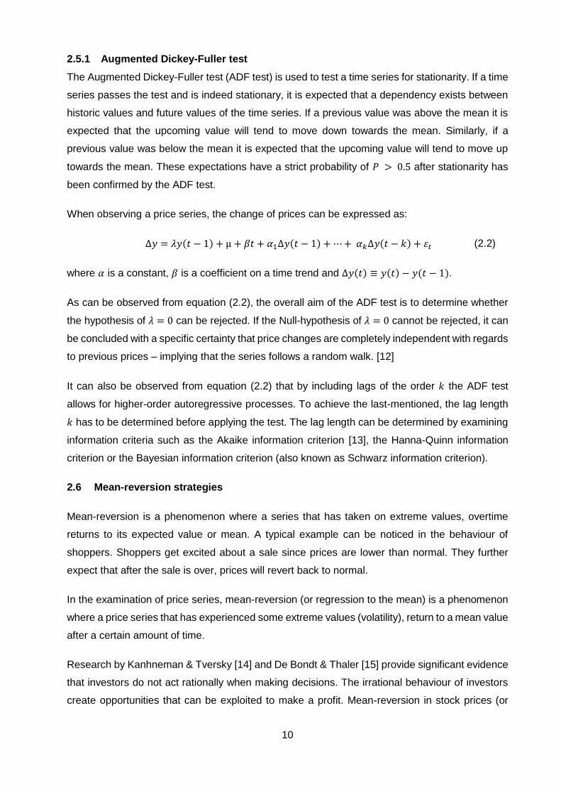
2.5.1 Augmented Dickey-Fuller test
The Augmented Dickey-Fuller test (ADF test) is used to test a time series for stationarity. If a time
series passes the test and is indeed stationary, it is expected that a dependency exists between
historic values and future values of the time series. If a previous value was above the mean it is
expected that the upcoming value will tend to move down towards the mean. Similarly, if a
previous value was below the mean it is expected that the upcoming value will tend to move up
towards the mean. These expectations have a strict probability of 𝑃 > 0.5 after stationarity has
been confirmed by the ADF test.
When observing a price series, the change of prices can be expressed as:
∆𝑦 = 𝜆𝑦(𝑡 − 1) + µ + 𝛽𝑡 + 𝛼1∆𝑦(𝑡 − 1) + ⋯+ 𝛼𝑘∆𝑦(𝑡 − 𝑘) + 휀𝑡 (2.2)
where 𝛼 is a constant, 𝛽 is a coefficient on a time trend and ∆𝑦(𝑡) ≡ 𝑦(𝑡) − 𝑦(𝑡 − 1).
As can be observed from equation (2.2), the overall aim of the ADF test is to determine whether
the hypothesis of 𝜆 = 0 can be rejected. If the Null-hypothesis of 𝜆 = 0 cannot be rejected, it can
be concluded with a specific certainty that price changes are completely independent with regards
to previous prices – implying that the series follows a random walk. [12]
It can also be observed from equation (2.2) that by including lags of the order 𝑘 the ADF test
allows for higher-order autoregressive processes. To achieve the last-mentioned, the lag length
𝑘 has to be determined before applying the test. The lag length can be determined by examining
information criteria such as the Akaike information criterion [13], the Hanna-Quinn information
criterion or the Bayesian information criterion (also known as Schwarz information criterion).
2.6 Mean-reversion strategies
Mean-reversion is a phenomenon where a series that has taken on extreme values, overtime
returns to its expected value or mean. A typical example can be noticed in the behaviour of
shoppers. Shoppers get excited about a sale since prices are lower than normal. They further
expect that after the sale is over, prices will revert back to normal.
In the examination of price series, mean-reversion (or regression to the mean) is a phenomenon
where a price series that has experienced some extreme values (volatility), return to a mean value
after a certain amount of time.
Research by Kanhneman & Tversky [14] and De Bondt & Thaler [15] provide significant evidence
that investors do not act rationally when making decisions. The irrational behaviour of investors
create opportunities that can be exploited to make a profit. Mean-reversion in stock prices (or
11
their returns) is a by-product of the behaviour of investors concerning the aversion of losses,
availability bias and affinity of lower prices.
Mean-reversion as a methodology can be used as a trading strategy. The concept of mean-
reversion trading is built on the assumption that a security’s high and low prices are only
temporary and that the series will revert to a certain mean value over time. [16]
Mean-reversion strategies can be more easily implemented when price series are stationary. The
price series of most securities are not stationary since prices are subject to drifts such as those
caused by trends and momentum. Even though single price series are seldom stationary, a
stationary price series can be obtained by creating a linear (weighted) combination of securities
that exhibit a certain relation.
A popular market-neutral trading strategy, pairs trading, was pioneered to exploit relations that
exist in the market. Securities that could be possible candidates for pairs trading can be found by
testing for relations such as correlation and/or cointegration.
2.7 Correlation and cointegration
Correlation and cointegration are related in statistical arbitrage, but are used to test for different
phenomena. Correlation refers to any of a broad class of statistical relationships involving
dependence while cointegration is a method that deals with the long-term relations between
security prices. A high correlation does not imply that security prices are highly cointegrated and
vice versa.
2.7.1 Correlation and dependence
In statistics, dependence is defined as any statistical relationship that may exist between two sets
of data (or two random variables). Correlation denotes the degree to which two or more sets of
data show a tendency to vary together. Correlations are very useful as they can be used to make
predictions. [17]
In the shopping example where customers are expected to buy more of a product that is on sale,
the manager of a store can make informed decisions when certain correlations are known. If a
certain product reaches its expiry date, the price could be lowered in order to boost the sales of
the product before it loses value. Statistical dependence however is not sufficient to assume a
causal relationship. In the shopping example, the store manager might expect that a sudden spike
in trading volume of a product on sale might be happening because of its lowered price, while in
reality there might be an entirely different reason.
12
There are several correlation coefficients that have been developed to measure the degree of
correlation. These coefficients are most commonly denoted 𝑝 or 𝑟. One of the most commonly
used correlation coefficients is Pearson’s product-moment coefficient, which is sensitive to only a
linear relationship between two variables. A linear relationship may exist even if one of the
variables is a nonlinear function of the other. [17]
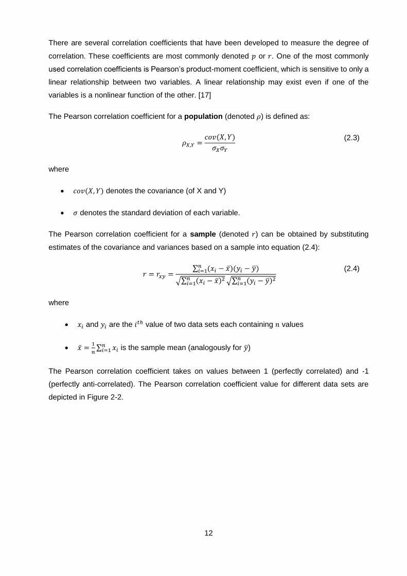
The Pearson correlation coefficient for a population (denoted 𝜌) is defined as:
𝜌𝑋,𝑌 =
𝑐𝑜𝑣(𝑋, 𝑌)
𝜎𝑋𝜎𝑌
(2.3)
where
𝑐𝑜𝑣(𝑋, 𝑌) denotes the covariance (of X and Y)
𝜎 denotes the standard deviation of each variable.
The Pearson correlation coefficient for a sample (denoted 𝑟) can be obtained by substituting
estimates of the covariance and variances based on a sample into equation (2.4):
𝑟 = 𝑟𝑥𝑦 =
∑ (𝑥𝑖 − �̅�)(𝑦𝑖 − �̅�)𝑛𝑖=1
√∑ (𝑥𝑖 − �̅�)2𝑛𝑖=1 √∑ (𝑦𝑖 − �̅�)2𝑛
𝑖=1
(2.4)
where
𝑥𝑖 and 𝑦𝑖 are the 𝑖𝑡ℎ value of two data sets each containing 𝑛 values
�̅� =1
𝑛∑ 𝑥𝑖
𝑛𝑖=1 is the sample mean (analogously for �̅�)
The Pearson correlation coefficient takes on values between 1 (perfectly correlated) and -1
(perfectly anti-correlated). The Pearson correlation coefficient value for different data sets are
depicted in Figure 2-2.

13
Figure 2-2: Pearson correlation coefficient for different data sets [18]
2.7.2 Testing for unit roots and cointegration
2.7.2.1 Autoregressive models
In the fields of statistics and signal processing, an autoregressive (AR) model is used to represent
a type of random process. It is commonly used to describe time-varying processes in nature and
economics. The autoregressive model stipulates that the output variable depends linearly on its
own previous values and an imperfectly predictable term (stochastic term). An AR model is usually
depicted in the form of a stochastic difference equation. The notation 𝐴𝑅(𝑝) indicates an
autoregressive model of order 𝑝. The 𝐴𝑅(𝑝) model is defined as
𝑋𝑡 = 𝑐 + ∑ 𝜑𝑖𝑋𝑡−𝑖 + 휀𝑡
𝑝
𝑖=1
(2.5)
where 𝜑1, … , 𝜑𝑝 are the parameters of the model, 𝑐 is a constant and 휀𝑡 is white noise. [19]
2.7.2.2 Unit root testing
A unit root test is used to determine if a time series is non-stationary by using an autoregressive
model. These tests normally declare as null hypothesis the existence of a unit root. A first order
autoregressive process 𝑋𝑡 = 𝑎𝑋𝑡−1 + 𝑒𝑡 where 𝑒𝑡 is white noise can also be expressed as:
𝑋𝑡 − 𝑎𝑋𝑡−1 = 𝑒𝑡 (2.6)
By using the backshift operator (𝐵), the model can be expressed as 𝑋𝑡(1 − 𝑎𝐵) = 𝑒𝑡. The
characteristic polynomial for the model is thus 1 − 𝑎𝐵. The polynomial has a unit root at 𝑎 = 1.

14
For |𝑎| < 1 the 𝐴𝑅(1) process is stationary and for |𝑎| > 1 the 𝐴𝑅(1) process is nonstationary.
When 𝑎 = 1, the process follows a random walk and is nonstationary. The unit roots can be
observed to form the boundary between stationary and nonstationary.
Intuitively, the occurrence of a unit root would allow a process that has deviated to not return to
its historic values (although the process will still shift around randomly). If the absence of a unit
root, the process will have a tendency to drift back to historic positions (while the random noise
will still have its effect). [20]
Some well-known unit root tests include the Augmented Dickey-Fuller test (section 2.4.1) and the
Phillips-Perron test.
2.7.2.3 Cointegration testing
Cointegration is a statistical method that can be used to determine if different price series have a
fixed relation over a certain time period. Cointegration is defined when the error term in regression
modelling is stationary. In mathematical terms, if two variables 𝑥𝑡 and 𝑦𝑡 are cointegrated, a linear
combination of them must be stationary such that:
𝑥𝑡 − 𝛽𝑦𝑡 = 𝑢𝑡 (2.7)
where 𝑢𝑡 is a stationary process. It can also be stated that if two or more series are individually
integrated and the order of integration1 between the series differ, the series are said to be
cointegrated. [21]
When a group of price series are found to be cointegrating, the relations tend to last for a longer
period and are better suited (than correlation) for traders that focus on pair trading. Alexander and
Dimitriu [2] present some arguments in favour of cointegration compared to correlation as a
measure of association in financial markets.
Some cointegration testing techniques include the Engle-Granger two-step method [22], the
Johansen test [23] and the Phillips-Ouliaris test. In contrast to the Engle-Granger method and
Phillips-Ouliaris test, the Johansen test can be used to test multiple time series for cointegration
and provide linear weights from the resulting eigenvectors to form stationary series.
1 Order of integration is a summary statistic that reports the minimum number of differences that is required to obtain a covariance stationary series. It is denoted 𝐼(𝑑).
15
2.7.2.4 Johansen cointegration test
In the field of statistics, the Johansen test [23] is a procedure for testing several 𝐼(1) time series
for cointegration. The test allows for more than one cointegrating relationship and is therefore
generally more applicable than the Engle-Granger test (which is based on the Dickey-Fuller test
for unit roots in the residuals from a single cointegrating relationship). The Johansen test will be
summarized in this section. See Johansen’s paper [23] and Appendix A for more details and
complete derivations.
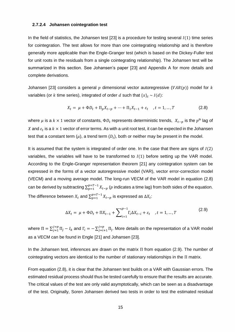
Johansen [23] considers a general 𝑝 dimensional vector autoregressive (𝑉𝐴𝑅(𝑝)) model for 𝑘
variables (or 𝑘 time series), integrated of order 𝑑 such that {𝑥}𝑡 ~ 𝐼(𝑑):
𝑋𝑡 = 𝜇 + Ф𝐷𝑡 + П𝑝𝑋𝑡−𝑝 + ⋯+ П1𝑋𝑡−1 + 휀𝑡 , 𝑡 = 1,… , 𝑇 (2.8)
where 𝜇 is a 𝑘 × 1 vector of constants, Ф𝐷𝑡 represents deterministic trends, 𝑋𝑡−𝑝 is the 𝑝th lag of
𝑋 and 휀𝑡 is a 𝑘 × 1 vector of error terms. As with a unit root test, it can be expected in the Johansen
test that a constant term (𝜇), a trend term (𝐷𝑡), both or neither may be present in the model.
It is assumed that the system is integrated of order one. In the case that there are signs of 𝐼(2)
variables, the variables will have to be transformed to 𝐼(1) before setting up the VAR model.
According to the Engle-Granger representation theorem [21] any cointegration system can be
expressed in the forms of a vector autoregressive model (VAR), vector error-correction model
(VECM) and a moving average model. The long-run VECM of the VAR model in equation (2.8)
can be derived by subtracting ∑ 𝑋𝑡−𝑝𝑝=𝑇−1𝑝=1 (𝑝 indicates a time lag) from both sides of the equation.
The difference between 𝑋𝑡 and ∑ 𝑋𝑡−𝑝𝑝=𝑇−1𝑝=1 is expressed as ∆𝑋𝑡:
∆𝑋𝑡 = 𝜇 + Ф𝐷𝑡 + Π𝑋𝑡−1 + ∑ Γ𝑖Δ𝑋𝑡−𝑖
𝑝−1
𝑖=1+ 휀𝑡 , 𝑡 = 1,… , 𝑇
(2.9)
where П = ∑ П𝑗 − 𝐼𝑘𝑗=𝑝𝑗=1 and Γ𝑖 = −∑ Πj
𝑗=𝑝𝑗=𝑖+1 . More details on the representation of a VAR model
as a VECM can be found in Engle [21] and Johansen [23].
In the Johansen test, inferences are drawn on the matrix П from equation (2.9). The number of
cointegrating vectors are identical to the number of stationary relationships in the П matrix.
From equation (2.8), it is clear that the Johansen test builds on a VAR with Gaussian errors. The
estimated residual process should thus be tested carefully to ensure that the results are accurate.
The critical values of the test are only valid asymptotically, which can be seen as a disadvantage
of the test. Originally, Soren Johansen derived two tests in order to test the estimated residual
16
process: the maximum eigenvalue test and the trace test [23]. These tests are used to check for
reduced rank of Π, which is a test for stationarity of the residual process.
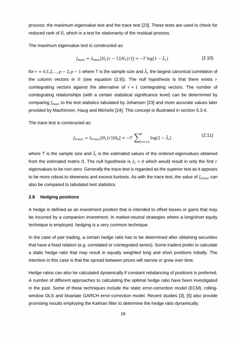
The maximum eigenvalue test is constructed as:
𝐽𝑚𝑎𝑥 = 𝜆𝑚𝑎𝑥[𝐻1(𝑟 − 1)|𝐻1(𝑟)] = −𝑇 log (1 − �̂�𝑟) (2.10)
for 𝑟 = 0,1,2, . . , 𝑝 − 2, 𝑝 − 1 where T is the sample size and �̂�𝑟 the largest canonical correlation of
the column vectors in Π (see equation (2.9)). The null hypothesis is that there exists 𝑟
cointegrating vectors against the alternative of 𝑟 + 1 cointegrating vectors. The number of
cointegrating relationships (with a certain statistical significance level) can be determined by
comparing 𝐽𝑚𝑎𝑥 to the test statistics tabulated by Johansen [23] and more accurate values later
provided by MacKinnon, Haug and Michelis [24]. This concept is illustrated in section 5.3.4.
The trace test is constructed as:
𝐽𝑡𝑟𝑎𝑐𝑒 = 𝜆𝑡𝑟𝑎𝑐𝑒[𝐻1(𝑟)|𝐻0] = −𝑇 ∑ log (1 − �̂�𝑖)
𝑝
𝑖=𝑟+1
(2.11)
where T is the sample size and �̂�𝑖 is the estimated values of the ordered eigenvalues obtained
from the estimated matrix Π. The null hypothesis is 𝜆𝑖 = 0 which would result in only the first 𝑟
eigenvalues to be non-zero. Generally the trace test is regarded as the superior test as it appears
to be more robust to skewness and excess kurtosis. As with the trace test, the value of 𝐽𝑡𝑟𝑎𝑐𝑒 can
also be compared to tabulated test statistics.
2.8 Hedging positions
A hedge is defined as an investment position that is intended to offset losses or gains that may
be incurred by a companion investment. In market-neutral strategies where a long/short equity
technique is employed, hedging is a very common technique.
In the case of pair trading, a certain hedge ratio has to be determined after obtaining securities
that have a fixed relation (e.g. correlated or cointegrated series). Some traders prefer to calculate
a static hedge ratio that may result in equally weighted long and short positions initially. The
intention in this case is that the spread between prices will narrow or grow over time.
Hedge ratios can also be calculated dynamically if constant rebalancing of positions is preferred.
A number of different approaches to calculating the optimal hedge ratio have been investigated
in the past. Some of these techniques include the static error-correction model (ECM), rolling-
window OLS and bivariate GARCH error-correction model. Recent studies [3], [5] also provide
promising results employing the Kalman filter to determine the hedge ratio dynamically.
17
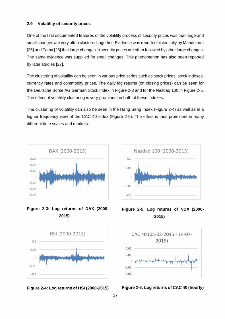
2.9 Volatility of security prices
One of the first documented features of the volatility process of security prices was that large and
small changes are very often clustered together. Evidence was reported historically by Mandelbrot
[25] and Fama [26] that large changes in security prices are often followed by other large changes.
The same evidence was supplied for small changes. This phenomenon has also been reported
by later studies [27].
The clustering of volatility can be seen in various price series such as stock prices, stock indexes,
currency rates and commodity prices. The daily log returns (on closing prices) can be seen for
the Deutsche Börse AG German Stock Index in Figure 2-3 and for the Nasdaq 100 in Figure 2-5.
The effect of volatility clustering is very prominent in both of these indexes.
The clustering of volatility can also be seen in the Hang Seng Index (Figure 2-4) as well as in a
higher frequency view of the CAC 40 index (Figure 2-6). The effect is thus prominent in many
different time scales and markets.
Figure 2-3: Log returns of DAX (2000-
2015)
Figure 2-4: Log returns of HSI (2000-2015)
Figure 2-5: Log returns of NDX (2000-
2015)
Figure 2-6: Log returns of CAC 40 (hourly)
-0.06
-0.04
-0.02
0
0.02
0.04
0.06
DAX (2000-2015)
-0.1
-0.05
0
0.05
0.1
HSI (2000-2015)
-0.1
-0.05
0
0.05
0.1
Nasdaq 100 (2000-2015)
-0.02
-0.01
0
0.01
0.02
CAC 40 (05-02-2015 - 14-07-2015)

18
2.10 Modelling volatility
2.10.1 Overview of ARCH models
Autoregressive conditional heteroskedasticity (ARCH) models have been developed to
characterize and model the empirical features of observed time series. These models are used if
there is reason to believe that the error terms in a time series have a characteristic size or variance
at any point in the series. ARCH and GARCH (generalized ARCH) models have grown to become
significant tools in the analysis of time series data. These models are particularly useful in financial
applications to analyse and forecast volatility. [28]
2.10.2 ARCH(q) model specification
An ARCH process can be used to model a time series. Let 휀𝑡 denote the return residuals with
respect to the mean process (error terms). These error terms can be divided into a stochastic part
(𝑧𝑡) and a time-dependent standard deviation (𝜎𝑡) such that:
휀𝑡 = 𝜎𝑡𝑧𝑡
The assumption is made that the random variable 𝑧𝑡 is a strong white noise process. The variance
(𝜎𝑡2) can be modelled by:
𝜎𝑡
2 = 𝛼0 + 𝛼1휀𝑡−12 + ⋯+ 𝛼𝑞휀𝑡−𝑞
2 = 𝛼0 + ∑ 𝛼𝑖휀𝑡−𝑖2
𝑞
𝑖=1
(2.12)
where 𝛼0 > 0 and 𝛼𝑖 ≥ 0 for 𝑖 > 0. Engle [29] proposed a methodology to test for the lag length
(𝑞) of ARCH errors using the Lagrange multiplier test.
2.10.3 GARCH(p,q) model specification
A generalized ARCH (or GARCH) model comes into existence when an autoregressive moving-
average (ARMA) model is assumed for the error variance. In this case the 𝐺𝐴𝑅𝐶𝐻(𝑝, 𝑞) model is
given by:
𝜎𝑡2 = 𝛼0 + 𝛼1휀𝑡−1
2 + ⋯+ 𝛼𝑞휀𝑡−𝑞2 + 𝛽1𝜎𝑡−1
2 + ⋯+ 𝛽𝑝𝜎𝑡−𝑝2 (2.13)
∴ 𝜎𝑡2 = 𝛼0 + ∑ 𝛼𝑖휀𝑡−𝑖
2𝑞
𝑖=1+ ∑ 𝛽𝑖𝜎𝑡−𝑖
2𝑝
𝑖=1
where p is the order of GARCH terms (𝜎2) and q is the order of ARCH terms (휀2). Details on the
parameter estimation and lag length calculation is provided in section 4.6.
19
2.11 Cluster analysis
Cluster analysis (or clustering) is a term used for techniques that group a set of objects with the
objective of ending up with groups that contain objects that are most similar to each other. Cluster
analysis forms a core part of exploratory data mining and is frequently used in statistical data
analysis. The use of cluster analysis can be found in machine learning, pattern recognition,
bioinformatics and data compression. [30]
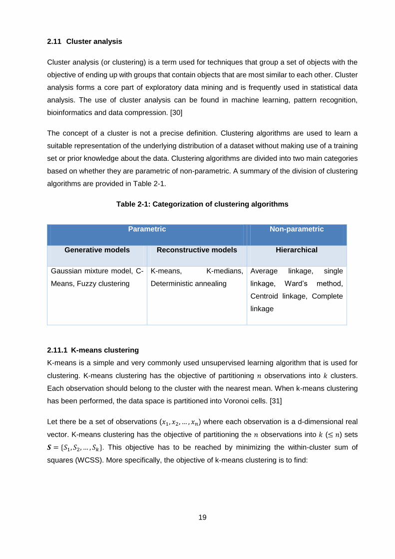
The concept of a cluster is not a precise definition. Clustering algorithms are used to learn a
suitable representation of the underlying distribution of a dataset without making use of a training
set or prior knowledge about the data. Clustering algorithms are divided into two main categories
based on whether they are parametric of non-parametric. A summary of the division of clustering
algorithms are provided in Table 2-1.
Table 2-1: Categorization of clustering algorithms
Parametric Non-parametric
Generative models Reconstructive models Hierarchical
Gaussian mixture model, C-
Means, Fuzzy clustering
K-means, K-medians,
Deterministic annealing
Average linkage, single
linkage, Ward’s method,
Centroid linkage, Complete
linkage
2.11.1 K-means clustering
K-means is a simple and very commonly used unsupervised learning algorithm that is used for
clustering. K-means clustering has the objective of partitioning 𝑛 observations into 𝑘 clusters.
Each observation should belong to the cluster with the nearest mean. When k-means clustering
has been performed, the data space is partitioned into Voronoi cells. [31]
Let there be a set of observations (𝑥1, 𝑥2, … , 𝑥𝑛) where each observation is a d-dimensional real
vector. K-means clustering has the objective of partitioning the 𝑛 observations into 𝑘 (≤ 𝑛) sets
𝑺 = {𝑆1, 𝑆2, … , 𝑆𝑘}. This objective has to be reached by minimizing the within-cluster sum of
squares (WCSS). More specifically, the objective of k-means clustering is to find:

20
arg𝑚𝑖𝑛
𝑠 ∑ ∑||𝑥 − µ𝑖||
2
𝑥∈𝑆𝑖
𝑘
𝑖=1
(2.14)
where µ𝑖 is the mean of points in 𝑆𝑖. In order to achieve equation (2.14), a number of heuristic
algorithms have been developed. The most common algorithm uses an iterative refinement
technique called Lloyd’s algorithm. When an initial set if k-means 𝑚1(1)
, … ,𝑚𝑘(1)
has been chosen
(they can be randomly chosen), the algorithm continues by alternating between two steps, namely
an assignment step and update step.
During the assignment step each observation is assigned to the closest cluster center. This
approach minimizes within-cluster sum of squares (WCSS). The WCSS is the squared Euclidean
distance, which is intuitively the nearest mean. The assignment step can be mathematically
expressed as:
𝑆𝑖(𝑡)
= {𝑥𝑝: ||𝑥𝑝 − 𝑚𝑖(𝑡)
||2
≤ ||𝑥𝑝 − 𝑚𝑗(𝑡)
||2
∀ 𝑗, 1 ≤ 𝑗 ≤ 𝑘}
where each observation (𝑥𝑝) is assigned to exactly one set (𝑆(𝑡)), even though it could be assigned
to more if the distances are the same.
During the update step, the new means to be the centroids of the observations in the new clusters
are calculated:
𝑚𝑖(𝑡+1)
=1
|𝑆𝑖(𝑡)
| ∑ 𝑥𝑗
𝑥𝑗∈𝑆𝑖𝑡
where 𝑥𝑗 is the is jth observation that belongs to the set 𝑆𝑖(𝑡)
and |𝑆𝑖(𝑡)
| indicates the number of data
points in the respective set. When the assignments of the observations do not change, the
algorithm has converged. The algorithm does not guarantee that a global optimum will be
reached.
2.11.2 Affinity propagation clustering
In the fields of statistics and data mining, affinity propagation is a clustering algorithm where,
unlike with k-means clustering, it is not required that the number of clusters have to be determined
or estimated a priori. Affinity propagation clustering focusses on a concept of message passing
between data points. Affinity propagation finds members of the input set that are representative
of clusters, called exemplars. [32]
21
The affinity propagation algorithm can be explained as follows. Let 𝑥1, … , 𝑥𝑛 be a set of data points
that has an unknown internal structure. Let 𝑠 be a function that quantifies the similarity between
any two points, such that 𝑠(𝑥𝑖, 𝑥𝑗) > 𝑠(𝑥𝑖 , 𝑥𝑘) if and only if 𝑥𝑖 is more similar to 𝑥𝑗 than to 𝑥𝑘.
The algorithm proceeds by alternating two message passing steps, updating two matrices:
The “responsibility” matrix 𝑹 has values 𝑟(𝑖, 𝑘) that quantify how well-suited 𝑥𝑘 is to serve
as the exemplar for 𝑥𝑖, relative to other candidate exemplars for 𝑥𝑖.
The “availability” matrix A contains values 𝑎(𝑖, 𝑘) that represent how “appropriate” it would
be for 𝑥𝑖 to pick 𝑥𝑘 as its exemplar, taking into account other points’ preference for 𝑥𝑘 as
an exemplar.
Both matrices R and A initially contain only zeros. The algorithms performs the following steps
iteratively:
Responsibility updates are sent:
𝑟(𝑖, 𝑘) ← 𝑠(𝑖, 𝑘) −𝑚𝑎𝑥
𝑘′ ≠ 𝑘{𝑎(𝑖, 𝑘′) + 𝑠(𝑖, 𝑘′)}
Availability is updated as follows:
𝑎(𝑖, 𝑘) ← min(0, 𝑟(𝑘, 𝑘) + ∑ 𝑚𝑎𝑥(0, 𝑟(𝑖′, 𝑘))𝑖′∉{𝑖,𝑘} ) for 𝑖 ≠ 𝑘 and
𝑎(𝑘, 𝑘) ← ∑ max(0, 𝑟(𝑖′, 𝑘))
𝑖′≠𝑘
2.12 Background review
In this section an introduction to high frequency trading (HFT), general arbitrage and statistical
arbitrage has been provided. Focus was placed on the reasoning behind statistical arbitrage with
emphasis on the concepts of stationarity and mean-reversion. Some objectives behind the
hedging of positions in financial trading was also studied. It was concluded that mean-reversion
strategies perform well in the presence of stationary price series (in the strict or weak forms of
stationarity).
Tests for association were reviewed such as different forms of correlation and cointegration. The
augmented Dickey-Fuller test was reviewed along with motivations for searching for unit roots in
autoregressive processes. The Johansen method was discussed with focus on the two
hypothesis tests that are used for finding stationarity in the residual process of a VECM.

22
Volatility clustering was discovered to be present in most financial price series. This phenomenon
exists when periods of high volatility and periods of low volatility can be observed. Some recent
examples of this phenomenon from different financial markets were examined. Different volatility
models were discussed and emphasis was placed on autoregressive conditional
heteroskedasticity (ARCH/GARCH) models.
Finally, clustering methods were briefly reviewed and categorized according to generative,
reconstructive and hierarchical models. Two specific clustering methods were examined namely
k-means clustering and affinity propagation clustering.
23
CHAPTER 3
LITERATURE REVIEW
3.1 Overview of literature review
The literature review starts with a brief study of the efficient market hypothesis and some of the
criticisms that is has received over time. Some of the arguments that have been made for
quantitative trading and active investment management over several periods are then explored.
Techniques used in statistical arbitrage is reviewed and special attention is given to three
statistical arbitrage models, namely the minimum distance method, a model based on arbitrage
pricing theory and finally a cointegration-based statistical arbitrage model.
Techniques for classifying (or clustering) securities by using only price data is reviewed. Attention
is especially placed on machine learning and clustering algorithms for this goal. Finally, the use
of different ARCH/GARCH models in recent studies is investigated for modelling and predicting
stock market volatility.
3.2 The efficient market hypothesis
In a very persuasive survey article in the 1970s, Eugene Fama [33] argued that markets are
efficient and that news spreads quickly, without delay, to be reflected in the prices of securities.
This argument was built on a hypothesis which Fama called the efficient market hypothesis
(EMH). If EMH holds true, then an investor cannot, using any techniques, pick certain securities
that would allow for greater returns than those that could be obtained using a randomly selected
portfolio of individual securities with comparable risk.
The efficient market hypothesis is associated with the construct of a random walk model. A
random walk model is used to describe or characterize a price series where each subsequent
price change represents a random departure from the previous price.
Many financial economists and statisticians believe that stock prices are at least partially
predictable. A study by Malkiel [34], concludes that markets cannot be completely efficient as the
collective judgement of investors are bound to make mistakes. He states that it can be expected
that some market participants will sometimes act irrational. Malkiel also argues from his work that
markets are not entirely efficient, but that the efficiency has improved over time. Grossman and
Stiglitz [35] argue that if the financial market is perfectly efficient, there will be no incentive for
professionals to uncover the information that gets so quickly reflected in market prices.

24
3.3 Arguments for quantitative trading and active investing
A large number of empirical studies conclude that security prices contradict the efficient market
hypothesis. Jegadeesh and Titman [36] investigated a trading strategy in 1993 that buys well-
performing stocks and sells poor-performing stocks. In their research they show excess returns
of 12% relative to the standard capital asset pricing model (CAPM). In another study by Chan,
Jegadeesh and Lakonishok in 1996 [37] an examination was done on the predictability of future
returns from past returns. They show that there is little evidence of subsequent reversals in the
returns of stocks with high price and earnings momentum, suggesting that a market only gradually
responds to new information.
A study by Dunis and Ho [38] suggests that long-short market neutral strategies can generate
steady returns under adverse market circumstances. Their study was focussed on cointegration-
based strategies on the Dow Jones EUROStoxx 50 index during the period of January 2002 to
June 2003. A study by Nobrega and Oliveira [39] was done in 2013 to investigate the effect of
various machine learning models on statistical arbitrage. They conclude that these models appear
to be significantly profitable with an average annual return of 23.58% for their extreme learning
machine (ELM) model in out-of-sample data.
In a recent publication (2012) by Fama and French [40], four regions were examined to see if
there are value premiums in average stock returns. They conclude that from the four regions
(North America, Europe, Japan and Asia specific), there are value premiums in average stock
returns that, excluding Japan, decrease with size. With the exclusion of Japan, they find that
returns momentum is present and spreads in average momentum returns also decrease from
smaller to bigger stocks. These findings suggest that momentum is an anomaly that exists in
financial markets and can be utilized to gain excess returns.
3.4 Established models for statistical arbitrage
In this section, well-known models that have been widely used for statistical arbitrage will be
reviewed. As with most trading models, numerous variations of existing statistical arbitrage ideas
have been developed. It can be expected that many of these models are proprietary and thus not
widely known. The models discussed in this section are the most commonly used and has been
published in a number of peer reviewed journals and books. These models provide a framework
for further improvements and variations. The models that will be reviewed include the minimum
distance method, arbitrage pricing theory (APT) model and the cointegration model.
3.4.1 Minimum distance method
The minimum distance method was first proposed by Gatev et al [6]. The application of the
minimum distance method consists of two distinguishable periods. Firstly, there is a pair formation

25
period and secondly a trading period. Gatev et al [6] decided in their study to arbitrarily choose a
ratio of 2:1 for the timespan of these periods e.g. a twelve months formation period and a six
months trading period.
During the pair formation period, a universe is decided upon. Each security in the universe is
paired with another by selecting a security that minimizes the sum of squared deviations
(Euclidean distance) between the two normalized price series. Gatev et al placed the restriction
on pairs that they have to belong to the same sector. When all securities have been paired, the
top pairs with the smallest distance is selected for the trading period. Of course, the number of
pairs to be selected has to be determined by the user of this model.
The next step of the minimum distance model is to select a trading strategy for opening and
closing positions. Gatev et al [6] illustrated the concept with a simple trading rule that enters a
long position in the lower-priced security and a short position in the higher-priced security when
the spread of the normalized security prices have diverged by more than two standard deviations.
The standard deviations are calculated from the spread of the normalized prices over the
formation period. The long and short positions are opened with equal monetary value (e.g. $100
long and $100 short). The positions are closed when the prices cross. When the trading period
ends, all positions are closed regardless of whether the prices have converged or not.
The empirical results that are provided by Gatev et al [6] with respect to the US equity market
over a period of 40 years (1962-2002) indicate an average annual excess return of up to 11% for
portfolios of pairs. The results suggest that the strategy could thus be profitable. The empirical
results suggest that increasing the number of pairs allow for less variance in portfolio growth and
increases the minimum realised return without significantly affecting the maximum realised return.
3.4.2 Arbitrage pricing theory model
Vidyamurthy [41] suggested that another method of detecting marketable pairs is to make use of
arbitrage pricing theory (APT) which was first suggested by Ross [42] to determine asset prices.
When the assumption is made that the law of one price hold and market participants have
homogenous expectations, it claims that the return on any security is linearly related to a set of
risk factors:
𝑟𝑖 = 𝑟𝑓 + ∑ 𝛽𝑖,𝑗𝑟𝑗
∗ + 𝜖𝑖
𝑘
𝑗=1
(3.1)
where 𝛽𝑖,𝑗 is the risk exposure of asset 𝑖 to risk factor 𝑗, 𝑟𝑗∗ is the return contribution of risk factor
𝑗 and 𝑟𝑓 is the risk-free return. The residual, 𝜖𝑖, can be interpreted as the return component arising
from the idiosyncratic or specific risk of asset 𝑖. The expected value of 𝜖𝑖 should be zero. There
are two constraints that should hold:

26
𝐸[𝜖𝑖𝜖ℎ] = 0 ∀ 𝑖 𝑎𝑛𝑑 ℎ, 𝑖 ≠ ℎ
𝐸[𝜖𝑖(𝑟𝑗∗ − 𝐸[𝑟𝑗
∗])] = 0 for all assets and risk factors
Consult Ross [42] for more details on arbitrage pricing theory. With regards to statistical arbitrage,
the assumption is made that securities with virtually identical risk exposures should yield
approximately equal returns. For this reason, it may be possible to detect tradable pairs by
investigating the risk exposure of the securities to particular risk factors.
Vidyamurthy [41] does not continue to specify which risk factors should be considered or how
exactly such a trading strategy should be executed. The assumption can be made that these
factors will have to be decided upon by the user of the model. Unlike the other models that are
discussed in this section, this strategy uses a well-known pricing theory underpinned by
fundamental economic reasoning. The model does make it clear that the objective of statistical
arbitrage strategies remains to find mispricings of very relatable securities. It does remain
questionable whether the APT model can be used sufficiently on its own as there is no restriction
placed on the hedge ratio of the pairs.
3.4.3 Cointegration for statistical arbitrage
In contrast to the minimum distance method described in section 3.4.1 which made no model
assumptions, the cointegration method is a model based parametric approach. The notion of the
cointegration approach is that if two security prices follow a common stochastic trend, the spread
between the securities may be weakly stationary. More precisely, if two security’s price series are
both integrated of order 𝑑 and there is a linear combination of the two price series that creates a
series which is integrated of order 𝑑 − 𝑏 where (𝑏 > 0), then the two series are considered
cointegrated (𝐶𝐼(𝑑, 𝑏)).
In the framework of statistical arbitrage, interest is placed on the situations where 𝑑 − 𝑏 = 0, such
that there exists a stationary time series for the spread. Many price series are integrated of order
1, 𝐼(1), and thus focus is placed on the situation where 𝑏 = 𝑑 = 1. A very advantageous part of
cointegrated price series, 𝑋𝑡 and 𝑌𝑡 is that these series can be represented in an error correction
model (ECM). In an ECM, the dynamics of one time series at a certain time point is a correction
of the last period’s deviation from the equilibrium with the addition of possible lag dynamics.
Harlacher [4] expresses this relation mathematically as:
∆𝑦𝑡 = 𝜓0 − 𝛾𝑦(𝑦𝑡−1 − 𝛼 − 𝛽𝑥𝑡−1) + ∑𝜓𝑥,𝑖Δ𝑥𝑡−𝑖
𝐾
𝑖=1
+ ∑𝜓𝑦,𝑖Δ𝑦𝑡−𝑖
𝐿
𝑖=1
+ 𝜖𝑦,𝑡 (3.2)
and similarly

27
∆𝑥𝑡 = 𝜉0 + 𝛾𝑥(𝑦𝑡−1 − 𝛼 − 𝛽𝑥𝑡−1) + ∑𝜉𝑦,𝑖Δ𝑦𝑡−𝑖
𝐾
𝑖=1
+ ∑𝜉𝑥,𝑖Δ𝑥𝑡−𝑖
𝐿
𝑖=1
+ 𝜖𝑥,𝑡 (3.3)
where 𝜖𝑦,𝑡 and 𝜖𝑥,𝑡 represents white noise and the terms ∆𝑦𝑡 and ∆𝑥𝑡 represents one period
differences in 𝑦𝑡 and 𝑥𝑡 respectively. If there is no deterministic trend in the series, the constants
𝜓 and 𝜉 are zero. The advantage of using an ECM is that active forecasts can be simply done by
using past information.
From equations (3.2) and (3.3) it is clear that the part that represents the deviation from the long-
run equilibrium is (𝑦𝑡−1 − 𝛼 − 𝛽𝑥𝑡−1). This term must be weakly stationary and the two coefficients
𝛾𝑦 and 𝛾𝑥 must have opposite algebraic signs. If this was not the case, there would be no error-
correcting behaviour. To test this phenomenon and for cointegration in general, one can follow
the procedure that was proposed by Engle and Granger [21]. This procedure consists of two
steps.
First, a linear regression is run of the one series on the other:
𝑦𝑡 = 𝛼 + 𝛽𝑥𝑡 + 휀𝑡 (3.4)
where 휀𝑡 is the error term. If the two variables are integrated of order one, the error term of the
regression must be weakly stationary (𝐼(0)). If this is the case, 𝑋 and 𝑌 are cointegrated. To test
for stationarity in the error term, the augmented Dickey-Fuller test (described in section 2.5.1) can
be used. Since the series to be tested is based on estimated coefficients, it is necessary to search
for the presence of a unit root in the residuals by using the critical values that are provided by
Phillips and Ouliaris [43].
An issue that arises is that it is unknown which security should be chosen as 𝑦𝑡 and which as 𝑥𝑡.
The choice matters in the test proposed by Engle and Granger [21]. It is therefore necessary to
test both ways.
Vidyamurthy [41] makes use of log-prices and does not necessarily base his trading model on the
cointegration condition. He, less strictly, searches for evidence of mean-reversion in the spread
time series that is defined as:
𝑚𝑡 = log(𝑃𝑡𝐴) − 𝛽log (𝑃𝑡
𝐵) (3.5)
If the two log priced are indeed cointegrated, the series in equation (3.5) can be expressed as:
𝑚𝑡 = 𝛼 + 𝜖𝑡 (3.6)

28
with respect to equation (3.3). This would indicate that the spread price series moves around the
equilibrium of 𝛼 as 𝜖𝑡 is assumed to be weakly stationary, but not necessarily identically and
independently distributed (i.i.d.).
From a trading perspective, it is not necessary that the spread series must be weakly stationary
in the strict statistical definition. It only needs to be mean-reverting for an effective trading rule to
be implementable. In contrast to the minimum distance rule, this model is not limited to trading
pairs, but it can also be generalised to more securities where a possible mean-reverting
equilibrium can exist.
3.5 Statistical arbitrage in different markets
Statistical arbitrage strategies aim to be market-neutral allowing for profits to be made in any type
of market situation. Avellaneda and Lee [44] have studied model-driven statistical arbitrage
strategies in the US equity market over the period of 1997 to 2007. Avellaneda and Lee focussed
on the use of principle component analysis (PCA) and sector ETFs by modelling the residuals
and idiosyncratic components of stock returns as a mean-reverting process. PCA-based
strategies achieved an average annual Sharpe ratio of 1.44 over the period.
A study by Caldeira and Moura [45] was done on a cointegration-based statistical arbitrage
strategy on the São Paulo stock exchange for the period of January 2005 to October 2012. Their
empirical analysis focussed on estimating long-term equilibrium and modelling the resulting
residuals. Their model obtained excess returns of 16.38% per annum with an average Sharpe
ratio of 1.34.
Some studies indicate the existence of statistical arbitrage opportunities in the term structure of
credit default swap (CDS) spreads. Jarrow and Li [46] estimated an affine model for the term
structure of CDS spreads on North American companies and identified mis-valued CDS contracts
along the credit curve. Their trading rules were contrarian by betting that mis-valuations will
disappear over time. Their empirical analysis concluded that the aggregate returns of the trading
strategy are positively related to the square of the market-wide credit and liquidity risk, indicating
that the CDS market is less competitive when it is more volatile.
The application of statistical arbitrage trading on US energy futures markets have been
investigated by Kanamura, Rachev and Fabozzi [47]. A simple pairs trading strategy was
implemented using a mean-reverting process of the futures price spread of specifically WTI crude
oil, heating oil and natural gas. Their results indicate that seasonality may be a prominent factor
in the profitability of the tested model and that certain pairs are more vulnerable to event risks.

29
3.6 Identifying related securities
When searching for possible statistical arbitrage opportunities, it may be necessary to group a
security universe into smaller subsets of related securities. These subsets can be pairs or larger
baskets. A common approach is to group securities by industry or sector. ETFs that track the
stock market of different countries can also form natural groups.
In some studies of statistical arbitrage, such as by Miao [48], a correlation matrix is calculated for
the entire universe. Filters are then applied by only selecting highly correlated securities to form
pairs for trading.
Clustering or classification algorithms can be used alongside descriptive features or statistics of
price series such as correlation and cointegration to obtain meaningful and related subsets. It is
often possible to obtain subsets this way that may have a fundamental economic relation without
having a priori knowledge of the relation.
It is possible to extract descriptive features from time series and then to perform clustering on
these features. Dueck and Frey [49] provide some arguments for using non-parametric clustering
methods with the introduction of a clustering algorithm called affinity propagation. Affinity
propagation is based on a concept of message passing between data points (described in section
2.11.2). In their study, Dueck and Frey argue that affinity propagation finds better solutions than
standard exemplar-based clustering algorithms such as k-medoids (a clustering algorithms
related to k-means algorithm and the mediodshift algorithm). They also shows that affinity
propagation can achieve similar results to vertex substitution heuristic (VSH) doing so in less
processing time for large datasets.
3.7 Predicting market volatility
The use of autoregressive conditional heteroskedasticity (ARCH) models for predicting market
volatility has received much attention in academic studies. Predicting volatility is very useful in
financial trading since it forms an integral part of risk management, asset allocation and for taking
bets on future volatility.
Alberg, Shalit and Yosef [50] estimated stock market volatility using asymmetric GARCH models.
They completed an empirical analysis of the mean return and conditional variance of Tel Aviv
Stock Exchange (TASE). Their results have shown that the asymmetric GARCH model with fat-
tailed densities improves the overall estimation for measuring conditional variance. The
exponential GARCH model using a skewed Student-t distribution proved to be most successful
for forecasting TASE indices.

30
Hung [51] applies an asymmetric GARCH model to the Taiwan weighted index (Taiwan), the
Nikkei 225 index (Japan) and Hang Seng index (Hong Kong). Although his GARCH model varies
from that of Alberg, Shalit and Yosef [50], he comes to a similar conclusion that volatility can be
more accurately modelled when provision is made for either positively or negatively skewed
returns.
Oberholzer [52] applied univariate GARCH, Glosten-Jagannathan-Runkle GARCH (GJR-
GARCH) and exponential GARCH (EGARCH) models to the JSE/FTSE stock indices over the
period of 2002 to 2014, especially noting results during the financial crisis. He concludes that the
GJR-GARCH model most effectively modelled the daily volatility of 5 South African indices on the
Johannesburg Stock Exchange (JSE). His results conclude similarly to Hung [51] and Alberg,
Shalit and Yosef [50] that asymmetric GARCH models tend to outperform other variations when
applied to index price series.
It can be concluded that if a deterministic trend is present in the price series, as is the case with
most stock indices, an asymmetric GARCH model should prove to be better than a standard
GARCH model at modelling volatility. It can be expected that the asymmetric GARCH models will
not provide an edge over standard GARCH models when modelling the volatility of (weakly)
stationary price series where no deterministic trend is present.
3.8 Literature review
In this section the efficient market hypothesis was discussed and arguments for and against the
hypothesis were provided. Some specific arguments for quantitative trading were reviewed. The
reviewed literature suggests that markets are not completely efficient and that certain exploitable
opportunities exist. The presence of anomalies with regards to the hypothesis were also reviewed.
Statistical arbitrage techniques were broadly reviewed and three specific methods were
discussed comprehensively. The literature suggests that a variety of statistical arbitrage
techniques can be profitable in a number of different financial markets.
The application of clustering techniques were reviewed and some specific methods with regards
to statistical arbitrage were studied. Literature regarding the application of volatility modelling on
different markets were reviewed and indications of better suited models for specific markets were
pointed out.

31
CHAPTER 4
METHODOLOGY
4.1 General overview of methodology
Statistical arbitrage of any form is reliant on securities that are related through an underlying
economic reason. This relation is not always easily known since many intricacies exist in the
financial market and data of these relations are in many cases not readily available. As an
example, a certain company might supply materials to another resulting in similar market
movements when the sales of the second company increases. Machine learning techniques that
are used for clustering or classification can be used to extract related securities from a large
dataset by studying only price series characteristics.
Cointegration methods have been widely used to identify and exploit potentially useful relations
in time series. When applied to price series in financial markets, it is possible to identify securities
with strong associations. The associations can in many cases be motivated by fundamental
economic reasons. As was explained in section 2.7.2.4, different cointegration tests exist. The
Johansen method is chosen as the cointegration test for this study since it allows for up to twelve
time series to be tested at once and it does not have to be re-run like the Engle-Granger test by
switching the dependant and independent variables.
The Johansen test provides a linear weighting of securities to produce a (weakly) stationary series
through the resulting eigenvectors. The stationary series is expected to have a joint probability
distribution that does not change over time. In section 2.9, it was shown that the volatility of price
series often cluster. It would thus be reasonable to expect that the weak stationary time series
obtained from the Johansen test can go through periods of high and low volatility.
Some trading strategies (see section 2.6) enter and exit trades based on rules that assume a
fixed standard deviation from the mean. Since volatility clusters, some trading opportunities can
be lost. Furthermore stop-loss orders can trigger unintelligently if based on a strategy that
assumes a fixed standard deviation.
In order to construct a more adaptable model for cointegration-based statistical arbitrage
techniques, a GARCH model will be constructed for modelling the volatility of the fabricated series
dynamically and thereby adjusting the thresholds for market decisions. The intention is to model
the dynamics of a mean-reverting portfolio more accurately in order to support a more optimal
application of trading rules.

32
Historic data sources of several exchanges are available for testing the proposed system (see
section 4.3). The proposed system will be tested on the different exchanges along with a classical
pairs trading strategy as was described in the study by Gatev et al [6]. This will provide a rich set
of results in order to scrutinize the developed models and validate the success rate of the
proposed system.
4.1.1 Chapter layout
This chapter consists of four main sections:
1. Description of models (section 4.2)
This section provides an overview of the proposed model and discusses the standard
pairs trading method that will be used for comparison as a benchmark.
2. Security universe and sampling frequency (section 4.3)
This section describes the data (type and granularity) that will be used for testing the
models.
3. Implementation of algorithms (sections 4.4 - 4.6)
All specifics regarding the implementation details of the various algorithms that were used
for constructing the proposed system are discussed in these sections. The sections
include the implementation of clustering techniques, the cointegration model and GARCH
model.
4. Performance evaluation metrics (section 4.7)
This section describes the metrics that were chosen for evaluating the performance of the
systems. The implementation of these risk metrics are also discussed.
4.1.2 Implementation approach
All models and algorithms will be developed in C++. Low level algebra will be done using Intel’s
Math Kernal Library (MKL) which provides high-speed implementations of LAPACK and BLAS.
The proposed system will be developed on a quantitative research platform that allows for
backtesting strategies, paper trading and live trading. The platform is able to manage several
portfolios and strategies simultaneously, making it possible to test the developed models on
several exchanges in parallel.

33
The following algorithms will be implemented and are discussed in this section:
1. Clustering methods (section 4.4)
a. K-means clustering
b. Affinity propagation clustering
2. Johansen cointegration test (section 4.5)
3. Generalised autoregressive conditional heteroskedasticity (GARCH) model (section 4.6)
a. Nelder-Mead simplex search for GARCH parameter estimation
4.2 Model descriptions
This section describes the two models that will be developed in this study. The first model will be
an implementation of the model described by Gatev et al [6]. This is referred to as the “standard
model” since this approach has been widely adopted for statistical arbitrage. The second model
(or the proposed system) makes use of a security clustering, cointegration testing and volatility
modelling. These underlying techniques will be discussed in this section. The second model is
also referred to as the adaptive model.
4.2.1 Implementation of the standard model
The standard model consists of two periods. The first period is called the “formation period” where
useful features are extracted from the data and pairs of similar securities are created. The second
period is referred to as the “trading period”. These two periods and the tasks that are performed
in them are discussed in sections 4.2.1.1 and 4.2.1.2.
4.2.1.1 Formation Period
Adjusted closing prices of the security universe are first normalized by using the following
algorithm:
Calculate the 1-period returns as 𝑟𝑡 = 1 +𝑦𝑡−𝑦𝑡−1
𝑦𝑡−1 where 𝑦𝑡 is the adjusted closing price at
time 𝑡 and 𝑟𝑡 is the 1-period return.
Calculate the compound product of each return vector such that 𝑃(𝑡 = 0) = 1
Calculate the mean (𝜇𝑟) and standard deviation (𝜎𝑟) of each compounded vector
Normalize the compounded vector by: 𝑟𝑡 =𝑟𝑡−𝜇𝑟
𝜎𝑟

34
When the security data has been normalized, it is necessary to calculate the squared-error (SE)
of all possible pairs and store these in a matrix 𝑆 such that 𝑆(𝑖, 𝑗) indicates the squared-error
between securities 𝑖 and 𝑗.
A number of best pairs for trading has to be chosen (𝑛𝑏). For each of the pairs with the smallest
SE values, a spread over the formation period is calculated as 𝑥𝑡 =𝑦𝑡𝑖
𝑦𝑡𝑗 where 𝑖 and 𝑗 indicate the
indices of the pairs in the matrix 𝑆. It has to be emphasized that the adjusted close prices are
used for calculating the spread and not the normalized return vectors that were previously
calculated. The moving average (𝜇𝑥) and standard deviation (𝜎𝑥) of the spread is calculated and
stored for use in the trading period.
4.2.1.2 Trading Period
In the trading period, the spread of each pair is calculated dynamically and a z-score is calculated
with regards to the moving average and standard deviation that were calculated in the formation
period:
𝑧 =𝑥 − 𝜇𝑥
𝜎𝑥
where 𝑥 is the latest spread of the 1-period returns. If the value of 𝑧 is higher or lower than a
certain threshold value, a market position is taken such that one security is bought and the other
is sold for the same value. A long position is taken in security with the lower return and a short
position is taken in the security with the higher return.
When the return spread has converged back to its average 𝜇𝑥 (such that the z-score crosses 0),
the long and short positions of the respective pair are closed. When the trading period ends, all
positions are closed whether the open positions have converged or not. The model then reverts
back to the formation period.
The free parameters and the default values (as chosen by Gatev et al [6]) of this model is
summarized below.
1. Formation period length (1 year)
2. Trading period length (1 semester)
3. Number of best pairs to trade (5)
4. Threshold value of z-score for entering/exiting market positions (2)

35
4.2.2 Implementation of adaptive model
Similar to the standard model, the proposed adaptive model also distinguishes between two
different periods. The first period is referred to as the “learning period” and the second period as
the “trading period”. The adaptive model trades baskets of securities as opposed to only pairs
and makes use of a clustering technique to identify related securities. Related securities are
tested for cointegration by using the Johansen method. The volatility of the baskets that are
considered for trading are also modelled. The implementation details of the adaptive model is
described is sections 4.2.2.1 and 4.2.2.2.
4.2.2.1 Learning period
4.2.2.1.1 Feature extraction and clustering
In the first part of the learning period, certain features have to be extracted from the time series
of the securities. These features will be used to cluster the securities into meaningful sets. The
adaptive model will make use of either k-means clustering or affinity propagation clustering. The
feature set used for k-means clustering is periodical returns of each price series. In the case of
affinity propagation, the similarity function will calculate the squared-error and correlation between
securities and use these values as measurements of similarity between the price series of
securities. Details about this clustering technique can be found in section 4.4.2.
The overall approach in the learning period is very similar to the pair selection of the standard
model, but it allows for baskets of securities up to a size of twelve. If any of the resulting clusters
contain more than twelve securities, they are respectively split in half until the resulting clusters
all contain less than thirteen securities.
4.2.2.1.2 Cointegration testing
The resulting clusters are tested for cointegration by making use of the Johansen method. The
Johansen method is constructed with a constant term and no deterministic trend (see section
4.5.6.1 for details). The number of lagged difference terms that will be examined follows a rolling
window of 1 ≤ 𝑘 ≤ 𝑡𝑟𝑎𝑑𝑖𝑛𝑔 𝑑𝑎𝑦𝑠 𝑖𝑛 𝑚𝑜𝑛𝑡ℎ. The approach of performing the Johansen test for
lags of up to a month allows for a search of various lag relations over time. The Johansen method
is not exhaustively performed for all values of 𝑘, but only until a cointegrating relation is found. It
is also possible to choose the lag term according to information criteria (e.g. Akaike information
criterion as in [48]), but this approach is not used in this study.
As an additional filter of the strength of the cointegrating relation, only baskets of securities that
have a 95% (statistical) certainty of having a cointegrating relation will be traded. The level of
certainty is calculated from the hypothesis tests described in section 4.5.6.1.

36
Once cointegrating relations have been found, the resulting eigenvectors from the Johansen test
are used to weigh the securities that form the stationary series. The weights can be used to
construct the stationary series for the timespan of the learning period. This part is later illustrated
in section 5.3.4. As an indication of the possible duration of the mean-reversion process, the
stationary series can be modelled as an Ornstein-Uhlenbeck process:
𝑑𝑦(𝑡) = (𝜆𝑦(𝑡 − 1) + 𝜇)𝑑𝑡 + 𝑑휀 (4.1)
where 𝑑휀 is Gaussian noise. The value of 𝜆 is calculated by linear regression. Chan [5] shows
that the half-life of mean-reversion for this process can then be calculated as:
𝑡ℎ𝑎𝑙𝑓−𝑙𝑖𝑓𝑒 = −
log(2)
𝜆
(4.2)
The value in equation (4.2) provides an indication of whether reversion to the mean is likely to
happen in an acceptable timeframe for the trader.
4.2.2.1.3 Modelling volatility of stationary series
The volatility of each stationary series will be modelled with the objective of dynamically updating
market entry thresholds. When the volatility of the weakly stationary series increase, the market
entry thresholds will increase. When the volatility of the series decreases, so will the entry
thresholds. This concept is similar to the working of a moving average filter.
The generalized autoregressive conditional heteroskedasticity (GARCH) model has been chosen
for modelling the volatility of the weakly stationary series. A GARCH model will be estimated for
each cointegrating relation that has been found by using the constructed stationary series over
the learning period.
In order to measure the fit of a GARCH model to the actual volatility, a persistency value can be
calculated by summing the estimated parameters. As an example, for a GARCH model that is
defined as (see equation (2.13)):
𝜎𝑡2 = 𝛼0 + ∑𝛼𝑖𝑋𝑡−𝑖
2
𝑝
𝑖=1
+ ∑𝛽𝑗𝜎𝑡−𝑗2
𝑞
𝑗=1
the persistency is calculated as the sum of ∑ 𝛼𝑖𝑝𝑖=1 + ∑ 𝛽𝑗
𝑞𝑗=1 where p is the order of GARCH terms
(𝜎2) and q is the order of ARCH terms (𝑋2). The persistency value is always bound between 0
and 1. A higher persistency value is preferred in this study as it corresponds to a better fit of the
GARCH model for this application. In this study, the GARCH model is only used when it has a
persistency value of higher than 0.9. If the GARCH model is not used to update the market entry

37
threshold, a default threshold of 1.5 deviations from the mean is used. Additional details regarding
the implementation of the GARCH model are described in section 4.6.
4.2.2.2 Trading period
With each new bar, the latest value of each stationary portfolio is calculated. For each stationary
portfolio, a z-score is calculated with regards to the moving average and standard deviation that
were calculated in the learning period:
𝑧 =𝑥 − 𝜇𝑥
𝜎𝑥
where 𝑥 is the latest value of the stationary portfolio. The z-score will be used for comparison with
the GARCH-updated volatility prediction to time the entry of market positions.
If the value of 𝑧 is higher than the GARCH-updated threshold value, a market position is taken
such that the stationary portfolio is effectively sold short. If the value of 𝑧 is lower than the negative
of the GARCH-updated threshold value, the stationary portfolio is bought.
When in a market position with the value of 𝑧 crossing zero, the long or short position in the
weighted (stationary) series is closed. When the trading period ends, all positions are closed. The
model then reverts back to the learning period.
The free parameters of this model is summarized below. The default values are chosen to be
similar to that of the standard model (see [6]).
1. Learning period length (1 year)
2. Trading period length (1 semester)
3. Number of baskets to trade (5)
4. Default deviation threshold when volatility model is not used (1.5)
4.3 Securities universe and sampling frequency
The data universe available for backtesting the two models include all existing securities from the
following exchanges:
New York stock exchange and Nasdaq (US)
Deutsche Börse Xetra (DE)

38
Tokyo stock exchange (JP)
Johannesburg stock exchange (SA)
Delisted securities are not considered in this study. Daily data is available for the entire timespan
that the securities have been listed on their respective exchanges. The study will however be
limited to the period of January 2006 to June 2016.
4.4 Implementation of clustering techniques
The k-means clustering and affinity propagation clustering algorithms were chosen for dividing a
large security universe into several smaller subsets that will be investigated for statistical arbitrage
opportunities. Both clustering techniques will be implemented and the better performing technique
will be used as default for this study. The techniques are compared in section 5.3.3.
The k-means clustering technique has the requirement of pre-specifying the number of clusters
to be obtained. This is useful as the number of subsets can be easily controlled when certain
trading restrictions are to be imposed. In contrast, the affinity propagation technique allows for
securities to be clustered into a varying number of groups, allowing for baskets of similar securities
to be obtained without placing a restriction.
4.4.1 Implementation of the k-means clustering algorithm
The standard k-means clustering algorithm was described in section 2.11.1. The algorithm will be
implemented for grouping pairs of similar securities. Prior to using k-means clustering, feature
extraction from the data will be necessary. In this study, fundamental data will not be used for
clustering the time series, but only the descriptive statistics of periodical returns. Statistics such
as correlation and squared-error cannot be used with k-means as these statistics are relative and
not absolute in nature.
In particular, the k-means++ clustering algorithm was chosen for this study. It is identical to the
standard k-means algorithm, with the exception of choosing initial centroids more intelligently (see
Arthur and Vassilvitskii [53]), rather than at random. The k-means implementation will now be
described in detail.
Given a matrix 𝐴 with dimensions 𝑛 × 𝑚, where 𝑛 is the number of (normalized) extracted features
and 𝑚 is the number of time series to be clustered, the k-means++ algorithm selects an initial
centroid at random. This centroid corresponds to a column in 𝐴 which is depicted as 𝑎0⃗⃗⃗⃗ . Assume
that a number of 𝑘 clusters are required from the data. The algorithm selects the remaining initial
centroids as follows:

39
1. For each column vector in 𝐴 (excluding chosen centroids) the distance between the vector
and all chosen centroids are calculated.
2. A new centroid is chosen as the vector that has the greatest distance from all chosen
centroids.
The steps above are repeated until 𝑘 initial centroids have been selected. The standard k-means
algorithm can now be followed:
1. Each observation (or column vector) in matrix 𝐴 is assigned to the nearest centroid in
terms of Euclidean distance.
2. New centroids are selected by calculating the mean of each cluster and assigning this
mean as the new centroid.
The above-mentioned steps are repeated until the clusters no longer changes, that is, the
observations are no longer assigned to different centroids. A maximum number of iterations is
defined for the algorithm such that execution will stop if the algorithm does not reach convergence.
4.4.2 Implementation of the affinity propagation clustering algorithm
The affinity propagation (AP) clustering algorithm was briefly described in section 2.11.2. This
algorithm is convenient as it can be used to select a number of clusters without requiring user
input such as with the k-means clustering algorithm. The term “exemplars” is used for existing
observations that are chosen as centers of the data, in contrast to “centroids” which do not
necessarily have to be actual observations and can be created (such as with k-means clustering).
As with the k-means clustering, it is required that certain descriptive features have to be extracted
from the time series. AP clustering makes use of a function 𝑠 that quantifies the similarity between
two points. In this study, the similarity function will be implemented as a similarity matrix 𝑆 with
𝑛 × 𝑛 dimensions that corresponds to 𝑛 time series to be clustered. Each value 𝑠𝑖𝑗 quantifies the
similarity between time series 𝑖 and 𝑗 (𝑖, 𝑗 = 1,2… , 𝑛).
This AP clustering implementation views each data point, 𝑠𝑖𝑗, as a node in a network. Messages
are recursively transmitted along the edges of a network until a good set of exemplars and
corresponding clusters emerge. The messages are updated on the basis of formulas that search
for minima of a chosen energy function, as will be shown in this section. At any point in time, the
magnitude of each message reflects the current affinity that one data point has for choosing
another data point as its exemplar. The details regarding the AP clustering implementation is
discussed in sections 4.4.2.1 to 4.4.2.5.

40
4.4.2.1 Building of initial graph
A graph object is constructed from a supplied similarity matrix. The graph contains all of the edges
between the vertices (data points). Each edge contains the following information:
Source and destination vertices
Similarity, responsibility and availability values between source and destination
When the graph is being constructed, preference values for exemplars are to be calculated. These
preference values are stored as the initial similarity value in all edges. Preference values ensure
that certain data points are more likely to be chosen as exemplars. The implementation for this
study contains three possible preference calculations:
1. Use the median of similarities as preference
2. Use the minimum of similarities as preference
3. Use the minimum – (maximum - minimum) of similarities as preference
If a priori, all data points are equally suitable as exemplars, the preferences should be set to a
common value according to Frey and Dueck [32]. Unless otherwise stated, the default preference
will be the median of similarities.
4.4.2.2 Clustering of data points
As with k-means clustering, AP clustering is an iterative process. The clustering halts when a
maximum iteration threshold number has been reached or when the clusters remain unchanged
for two consecutive iterations.
During each iteration, two main steps are performed: responsibility updating and availability
updating. Each of these steps take into account a different kind of competition, but remain
focussed on the concept of message passing. Messages can be combined at any stage to
determine which points are exemplars and (for non-exemplar points) to which exemplar each
point belongs.
4.4.2.3 Responsibility updates
The “responsibility” update is denoted 𝑟(𝑖, 𝑘) and is sent from data point 𝑖 to exemplar 𝑘. It is a
quantity that indicates how well-suited point 𝑘 is to serve as the exemplar for point 𝑖, taking
account of other potential exemplars for point 𝑖. The “availability” update is denoted 𝑎(𝑖, 𝑘) and is
sent from a candidate exemplar 𝑘 to point 𝑖. The availability update is a quantity that reflects the

41
accumulated evidence for how appropriate it would be for point 𝑖 to choose point 𝑘 as its exemplar,
taking into account the support from other points that point 𝑘 should be an exemplar.
The updates 𝑟(𝑖, 𝑘) and 𝑎(𝑖, 𝑘) can be viewed as log-probability ratios. Initially, all 𝑎(𝑖, 𝑘) values
are equal to zero. The responsibilities are computed using the following rule:
𝑟(𝑖, 𝑘) ← 𝑠(𝑖, 𝑘) −𝑚𝑎𝑥
𝑘′ ≠ 𝑘{𝑎(𝑖, 𝑘′) + 𝑠(𝑖, 𝑘′)} (4.3)
In the first iteration of the algorithm, 𝑟(𝑖, 𝑘) is set to the input similarity between points 𝑖 and 𝑘
minus the largest similarity between point 𝑖 and other candidate exemplars since all availability
values will be zero. The update rule of responsibility values is data-driven and does not consider
how many other points favour each candidate exemplar. This allows for no restrictions on the
amount of points per cluster. When 𝑘 = 𝑖 in equation (4.3), the responsibility is set to the input
preference that point 𝑘 is chosen as an exemplar. This “self-responsibility” value reflects the
gathered evidence that point 𝑘 is an exemplar, based on the input preference adjusted by how
unsuited it is to be assigned to another exemplar.
A damping factor is introduced (for this implementation) to the simple update rule in equation (4.3)
such that the responsibility values will actually be updated by:
𝑟(𝑖, 𝑘) = 𝜆𝑟𝑜(𝑖, 𝑘) + (1 − 𝜆)𝑟𝑛(𝑖, 𝑘) (4.4)
where 𝜆 is the damping factor, 𝑟𝑜(𝑖, 𝑘) is the old responsibility value and 𝑟𝑛(𝑖, 𝑘) is the new value
calculated by equation (4.3). The introduction of a damping factor ensures that oscillations that
will “overshoot” the solution are lessened (see [32] and [54] for details).
In later iterations when some points have been assigned to other exemplars, their availability
values will drop below zero. The negative availability values will decrease the effective values of
some of the input similarities 𝑠(𝑖, 𝑘′) in equation (4.3) which will remove the corresponding
candidate exemplars from competition.
4.4.2.4 Availability updates
In contrast to the responsibility update, which let candidate exemplars compete for ownership of
a data point, the availability update gathers evidence from the data points as to whether each
candidate exemplar would make a good exemplar. The availability update rule is defined as:
𝑎(𝑖, 𝑘) ← min(0, 𝑟(𝑘, 𝑘) + ∑ 𝑚𝑎𝑥(0, 𝑟(𝑖′, 𝑘))
𝑖′∉{𝑖,𝑘}
)
(4.5)
42
As can be seen from equation (4.5), the availability 𝑎(𝑖, 𝑘) is set to the addition of the self-
responsibility 𝑟(𝑘, 𝑘) and the sum of the positive responsibilities candidate exemplar 𝑘 receives
from other points. According to [32], only the positive incoming responsibilities are added because
it is only essential for a good exemplar to explain some of the data points well (i.e. positive
responsibilities) regardless of how poorly it explains other data points (i.e. negative
responsibilities).
The self-responsibility 𝑟(𝑘, 𝑘) can have a negative value that indicates that it would be better
suited for point 𝑘 to belong to another exemplar as to serve as an exemplar itself. In such a case
the availability of point 𝑘 as an exemplar can be increased if some other points have positive
responsibilities for point 𝑘 being their exemplar. To limit the effect of prominent incoming positive
responsibilities, the total sum is thresholded so that it cannot have a value above zero.
The self-availability 𝑎(𝑘, 𝑘) is updated as follows:
𝑎(𝑘, 𝑘) ← ∑ 𝑚𝑎𝑥(0, 𝑟(𝑖′, 𝑘))
𝑖′∉{𝑖,𝑘}
(4.6)
Equation (4.6) reflects gathered evidence that point 𝑘 is an exemplar, based on the positive
responsibilities sent to candidate exemplar 𝑘 from other points. As with the responsibility updates
in section 4.4.2.3, a damping factor is again introduced to avoid numerical oscillations that may
arise by updating the availability values in equations (4.5) and (4.6) as follows:
𝑎(𝑖, 𝑘) = 𝜆𝑎𝑜(𝑖, 𝑘) + (1 − 𝜆)𝑎𝑛(𝑖, 𝑘) (4.7)
where 𝜆 is the damping factor, 𝑎𝑜(𝑖, 𝑘) is the old availability value and 𝑎𝑛(𝑖, 𝑘) is the newly
calculated availability value.
4.4.2.5 Considerations of AP clustering
The implemented update rules perform simple computations and messages are only exchanged
between points with known similarities. It is thus possible to have situations where unknown
similarities may exist, in which case the algorithm is still able to perform clustering on the known
data.
At any point during the AP clustering iterations, availabilities and responsibilities can be combined
to identify exemplars. For point 𝑖 the value of 𝑘 that maximizes 𝑎(𝑖, 𝑘) + 𝑟(𝑖, 𝑘) either identifies the
data point that is the exemplar for point 𝑖 or it identifies point 𝑖 as an exemplar if 𝑘 = 𝑖.
The damping factor 𝜆 may have a value between 0.5 and 1, but will as default be 0.5 unless
otherwise stated in this research.

43
The affinity propagation clustering algorithm can be summarized as follows:
4.5 Implementation of the Johansen cointegration test
4.5.1 Overview of the Johansen test
The Johansen test for cointegration of time series was briefly discussed in section 2.7.2.4 and a
full derivation is supplied in Appendix A. The Johansen test is also referred to as “full-information
maximum likelihood” in some literature. An implementation of the Johansen test for this study will
be used to identify cointegrating price series for up to twelve securities which could be combined
to form a stationary series.
4.5.2 Review of the Johansen method
Let 𝑦𝑡 be an 𝑛 × 1 column vector containing the values at time 𝑡 of 𝑛 time series. The Johansen
method expects that 𝑦𝑡 can be expressed as a VAR(p) model:
𝑦𝑡 = 𝑐 + Ф1𝑦𝑡−1 + ⋯+ Ф𝑝𝑦𝑡−𝑝 + 휀𝑡 (4.8)
where 𝑐 is an (𝑛 × 1) vector, Ф𝑖 is an 𝑛 × 𝑛 matrix and 휀𝑡 is an error term. The model in equation
(4.8) indicates that each variable in 𝑦𝑡 has an equation explaining its evolution based on its own
lags and the lags of the other model variables. For the sake of clarity to readers unfamiliar with
VAR models, equation (4.8) for the case of two variables and 𝑝 = 1 will appear as:
Input:
similarities 𝑠𝑛𝑠→𝑛𝑡
preferences 𝑠𝑛𝑠→𝑛𝑠
Initialization:
set 𝑎𝑛𝑠→𝑛𝑡= 𝑟𝑛𝑠→𝑛𝑡
= 0 for all 𝑛𝑠 and 𝑛𝑡 ∈ [1,… ,𝑁]
Iteration:
while not converged do
update responsibilities
𝑟𝑛𝑠→𝑛𝑡 𝑠𝑛𝑠→𝑛𝑡− max𝑚𝑡≠𝑛𝑡
[𝑎𝑛𝑠→𝑚𝑡+ 𝑠𝑛𝑠→𝑚𝑡
] =𝜆
update availabilities
𝑎𝑛𝑠→𝑛𝑡 min {0, 𝑟𝑛𝑡→𝑛𝑡
+ ∑ max [0, 𝑟𝑚𝑠→𝑛𝑡]
𝑚𝑠≠{𝑛𝑠,𝑛𝑡}}=
𝜆
𝑎𝑛𝑡→𝑛𝑡 ∑ [0, 𝑟𝑚𝑠→𝑛𝑡
]𝑚𝑠≠𝑛𝑡
=𝜆

44
[𝑦1,𝑡
𝑦2,𝑡] = [
𝑐1𝑐2
] + [Ф1,1 Ф1,2
Ф2,1 Ф2,2] [
𝑦1,𝑡−1
𝑦2,𝑡−1] + [
𝑒1,𝑡
𝑒2,𝑡]
The model in equation (4.8) can be rewritten as (see Appendix B):
𝑦𝑡 = 𝑐 + 𝜌𝑦𝑡−1 + 𝛽1∆𝑦𝑡−1 + ⋯+ 𝛽𝑝−1∆𝑦𝑡−𝑝+1 + 휀𝑡 (4.9)
where Δ𝑦𝑡 = 𝑦𝑡 − 𝑦𝑡−1, 𝜌 = Ф1 + Ф2 + ⋯+ Ф𝑝 and
𝛽𝑖 = −(Ф𝑖+1 + Ф𝑖+2 + ⋯+ Ф𝑝), 𝑓𝑜𝑟 𝑖 = 1,2,… , 𝑝 − 1.
By subtracting 𝑦𝑡−1 from both sides of equation (4.9), the following equation is obtained:
∆𝑦𝑡 = 𝑐 + 𝛽0𝑦𝑡−1 + 𝛽1∆𝑦𝑡−1 + ⋯+ 𝛽𝑝−1∆𝑦𝑡−𝑝+1 + 휀𝑡 (4.10)
with
𝐸(휀𝑡) = 0
𝐸(휀𝑡휀𝜏) = {Ω for t = τ
0 𝑜𝑡ℎ𝑒𝑟𝑤𝑖𝑠𝑒
The above statement indicates that the contemporaneous covariance matrix of error terms is
Ω (a 𝑛 × 𝑛 positive-semidefinite matrix2). Johansen [23] showed that under the null hypothesis of
ℎ cointegrating relations, only ℎ separate linear combinations of 𝑦𝑡 appear in equation (4.10).
Johansen’s work implies that 𝛽0 in equation (4.10) can be expressed in the form:
𝛽0 = −𝐵𝐴′ (4.11)
where 𝐵 is an 𝑛 × ℎ matrix and 𝐴′ is an (ℎ × 𝑛) matrix.
Consider a sample of 𝑇 + 𝑝 observations symbolised as 𝑦−𝑝+1, 𝑦−𝑝+2, … , 𝑦𝑇. If the errors 휀𝑡 are
Gaussian, the log likelihood of 𝑦1, 𝑦2, … , 𝑦𝑇 conditional on 𝑦−𝑝+1, 𝑦−𝑝+2, … , 𝑦0 is given by:
2 A 𝑛 × 𝑛 real matrix 𝐴 is positive semi-definite if the scalar 𝑣𝑇𝐴𝑣 is zero or positive for every non-zero column vector 𝑣 of 𝑛 real numbers.

45
ℒ(Ω, 𝑐, 𝛽0, 𝛽1, … , 𝛽𝑝−1)
=−𝑇𝑛
2log(2𝜋) −
𝑇
2log|Ω|
−1
2∑[(Δ𝑦𝑡 − 𝑐 − 𝛽0𝑦𝑡−1 − 𝛽1Δ𝑦𝑡−1 − ⋯− 𝛽𝑝−1Δ𝑦𝑡−𝑝+1)
′𝑇
𝑡=1
× Ω−1(∆𝑦𝑡 − 𝑐 − 𝛽0𝑦𝑡−1 − 𝛽1∆𝑦𝑡−1 − ⋯− 𝛽𝑝−1∆𝑦𝑡−𝑝+1)]
(4.12)
The objective is to choose (Ω, 𝑐, 𝛽0, 𝛽1, … , 𝛽𝑝−1) such that equation (4.12) is maximized with the
constraint of being able to express 𝛽 in the form of equation (4.11). The Johansen method
calculates the maximum likelihood estimates of (Ω, 𝑐, 𝛽0, 𝛽1, … , 𝛽𝑝−1).
4.5.3 Johansen method: Input
The Johansen method is supplied with three variables:
A 𝑛 × 𝑚 matrix 𝑦𝑡 containing the time series that are to be tested for cointegration where
there are 𝑚 time series with 𝑛 data points
A parameter 𝑝 indicating the order of the time polynomial in the null hypothesis:
o If 𝑝 = −1, there is no constant or time-trend
o If 𝑝 = 0, there is only a constant term
o If 𝑝 = 1, there is a constant and a time-trend
A parameter 𝑘 that represents the number of lagged difference terms to be used when
computing the estimator
4.5.4 Johansen method: Step 1
In the first step of the Johansen cointegration test it is necessary to estimate a VAR(𝑝 − 1) model
for the matrix ∆𝑦𝑡. This task can be done by regressing ∆𝑦𝑖𝑡 on a constant and all elements of the
vectors ∆𝑦𝑡−1, … , ∆𝑦𝑡−𝑝+1 with ordinary least squares (OLS). The steps to achieving this is
discussed next.
The time series matrix 𝑦𝑡 is first detrended according to the value of 𝑝. A time differenced matrix
of 𝑦𝑡 is calculated by:
𝛿𝑦𝑡 = {0 , 𝑡 < 2
𝑦𝑡 − 𝑦𝑡−1, 𝑡 = 2,… , 𝑛

46
Notice that the first row of 𝛿𝑦𝑡 is zero since differences cannot be calculated on the first values.
The first row of zero values is not of use and is removed from 𝛿𝑦𝑡. Next a matrix 𝑧𝑡 is calculated
which contains the time-lagged values of 𝛿𝑦𝑡. The input parameter 𝑘 is used to determine the
number of time lags which will be contained in matrix 𝑧𝑡:
𝑧𝑡 = 𝑧𝑖,𝑡−1, 𝑧𝑖,𝑡−2, … , 𝑧𝑖,𝑡−𝑘 , 𝑖 = 1,2,… ,𝑚
where 𝑚 is the number of column vectors in 𝛿𝑦𝑡. The first 𝑘 rows of both matrices 𝛿𝑦𝑡 and 𝑧𝑡 are
removed and the matrices are detrended. It is now possible to achieve the objective of the first
step of the Johansen test by performing two regressions to obtain the residual processes.
As explained in section 4.5.2, if the series in 𝑦𝑡 are cointegrated, there exists a VECM
representation of the cointegrated system (equation (4.10)):
∆𝑦𝑡 = 𝑐 + 𝛽0𝑦𝑡−1 + 𝛽1∆𝑦𝑡−1 + ⋯+ 𝛽𝑝−1∆𝑦𝑡−𝑝+1 + 휀𝑡
where 𝛽0 = −𝐵𝐴′ has reduced rank 𝑟 which indicates the number of cointegrating vectors. Since
interest is placed on 𝛽0, it is more convenient to model 𝛽1, … , 𝛽𝑝−1 by a partial regression.
First, 𝛿𝑦𝑡 is regressed on 𝑧𝑡 = 𝑐 + 𝛽1∆𝑦𝑡−1 + ⋯+ 𝛽𝑝−1∆𝑦𝑡−𝑝+1 with the objective of obtaining the
residuals matrix 𝑟0𝑡:
𝑟0𝑡 = 𝛿𝑦𝑡 − 𝑧𝑡 × 𝑂𝐿𝑆(𝑧𝑡 , 𝛿𝑦𝑡) (4.13)
where 𝑂𝐿𝑆 indicates the application of ordinary least squares. The second regression will be of
𝑦𝑡−1 on 𝑧𝑡 = 𝑐 + 𝛽1∆𝑦𝑡−1 + ⋯+ 𝛽𝑝−1∆𝑦𝑡−𝑝+1. Before the second regression step can be
performed, it is necessary to calculate the 𝑘-lagged lagged matrix 𝑦𝑡−𝑘 as follows:
Obtain the 𝑘-lagged matrix of the input matrix
Remove the 𝑘 + 1 first rows from the obtained matrix
Detrend the obtained matrix with respect to the parameter input 𝑝
The residuals matrix 𝑟𝑘𝑡 can now be calculated as follows:
𝑟𝑘𝑡 = 𝑦𝑡−𝑘 − 𝑧𝑡 × 𝑂𝐿𝑆(𝑧𝑡 , 𝑦𝑡−𝑘) (4.14)
The residual processes have now been obtained and further inference will be drawn on these
matrices in section 4.5.5.

47
4.5.5 Johansen method: Step 2
The second step of the Johansen test is to calculate the sample covariance matrices of the OLS
residuals 𝑟0𝑡 and 𝑟𝑘𝑡 and find the eigenvalues of these covariance matrices. The sample
covariance matrices are calculated as:
𝑠𝑘𝑘 =
1
𝑇∑𝑟𝑘𝑡𝑟𝑘𝑡
′
𝑇
𝑡=1
(4.15)
𝑠00 =
1
𝑇∑𝑟0𝑡𝑟0𝑡
′
𝑇
𝑡=1
(4.16)
𝑠0𝑘 =
1
𝑇∑𝑟0𝑡𝑟𝑘𝑡
′
𝑇
𝑡=1
(4.17)
𝑠𝑘0 = 𝑠0𝑘′ (4.18)
where T is the size of the matrices 𝑟0𝑡 and 𝑟𝑘𝑡. To further investigate the properties of the sample
covariance matrices, Johansen [23] performs an eigenvalue decomposition of the matrix:
𝑠𝑘𝑘−1𝑠𝑘0𝑠00
−1𝑠0𝑘 (4.19)
The eigenvalues are sorted from largest to smallest and their corresponding eigenvectors are
also ordered according to the eigenvalues: �̂�1 > �̂�2 > ⋯ > �̂�𝑛. The maximum value of the log
likelihood function in equation (4.12), subject to the constraint that there exists ℎ cointegrating
relations, can be expressed as:
ℒ0∗ = −
𝑇𝑛
2log(2𝜋) −
𝑇𝑛
2−
𝑇
2log|𝑠00| −
𝑇
2∑log(1 − �̂�𝑖)
ℎ
𝑖=1
(4.20)
4.5.6 Johansen method: Step 3
In the third step of the Johansen cointegration test, the maximum likelihood estimates of the
parameters are calculated. Let the 𝑛 × 1 eigenvectors associated with the ℎ largest eigenvalues
of equation (4.19) be denoted �̂�1, … , �̂�ℎ. The eigenvectors provide a basis for the space of
cointegrating relations. The maximum likelihood estimate is that a cointegrating vector can be
written in the form:
𝑎 = 𝑏1�̂�1 + 𝑏2�̂�2 + ⋯+ 𝑏ℎ�̂�ℎ

48
where 𝑏1, … , 𝑏ℎ are scalars. Johansen [23] made the suggestion that the vectors �̂�𝑖 should be
normalized such that �̂�𝑖′𝑠𝑘𝑘�̂�𝑖 = 1. The ℎ normalized vectors are inserted into an 𝑛 × ℎ matrix �̂� =
[�̂�1 �̂�2 … �̂�ℎ]. The maximum likelihood estimate of 𝛽0 from equation (4.10) can be expressed as:
�̂�0 = 𝑠0𝑘�̂��̂�′
The maximum likelihood of 𝑐 in equation (4.10) is given by:
�̂� = �̂�0 − �̂�0
4.5.6.1 Hypothesis testing
The hypothesis testing of the Johansen method is discussed in this section. The null hypothesis
states that there are exactly ℎ cointegrating relations. In this case, the largest value of the log
likelihood function is given by equation (4.20). The alternative hypothesis is that there are 𝑛
cointegrating relations. The alternative hypothesis implies that every linear combination of 𝑦𝑡 is
stationary, which entails that 𝑦𝑡−1 would appear in equation (4.10) without constraints and no
restrictions will be placed on 𝛽0. The value of the log likelihood function in the absence of
constraints is given by:
ℒ1
∗ = −𝑇𝑛
2log(2𝜋) −
𝑇𝑛
2−
𝑇
2log|𝑠00| −
𝑇
2∑log(1 − �̂�𝑖)
𝑛
𝑖=1
(4.21)
The first likelihood ratio test of ℋ0: ℎ 𝑟𝑒𝑙𝑎𝑡𝑖𝑜𝑛𝑠 against the alternative ℋ1: 𝑛 𝑟𝑒𝑙𝑎𝑡𝑖𝑜𝑛𝑠 is based on
2(ℒ1
∗ − ℒ0∗) = −𝑇 ∑ log(1 − �̂�𝑖)
𝑛
𝑖=ℎ+1
(4.22)
The test in equation (4.22) is referred to as the trace test by Johansen [23].
A likelihood ratio test of ℋ0: ℎ 𝑟𝑒𝑙𝑎𝑡𝑖𝑜𝑛𝑠 against the alternative ℋ1: ℎ + 1 𝑟𝑒𝑙𝑎𝑡𝑖𝑜𝑛𝑠 is based on
2(ℒ1∗ − ℒ0
∗) = −𝑇 log(1 − �̂�ℎ+1) (4.23)
The test in equation (4.23) is referred to as the maximum eigenvalue test.
As was discussed briefly in section 4.5.3, there are three possible cases that the Johansen test
has to consider:
𝐶𝑎𝑠𝑒 1: The true value of the constant 𝑐 in equation (4.9) is zero. This means that there is no
intercept in any of the cointegrating relations and that no deterministic time trend is present in the
49
elements of 𝑦𝑡. In this case there is no constant term included in the regressions performed in
section 4.5.4.
𝐶𝑎𝑠𝑒 2: The true value of the constant in 𝑐 in equation (4.9) is such that there are no deterministic
time trends in any of the elements of 𝑦𝑡. In this case there are no restrictions on the constant term
in the estimation of the regressions in section 4.5.4.
𝐶𝑎𝑠𝑒 3: The true value of the constant in 𝑐 in equation (4.9) is such that there are deterministic
time trends in the elements of 𝑦𝑡. In this case there are no restrictions on the constant term in the
regressions in section 4.5.4.
The critical values for the trace and maximum eigenvalue tests in equations (4.22) and (4.23) are
found in the tabulations that were estimated by MacKinnon, Haug, and Michelis [24]. These critical
values allow for the tests to have a certain statistical significance level such as 90%, 95% and
99%. If not explicitly mentioned in further parts of the study, the default setup for the Johansen
test will be that of case 1, mentioned in this section.
4.6 Implementation of GARCH model
4.6.1 Overview of GARCH models
GARCH models are used to model and forecast the volatility (𝜎𝑡) of a time series. Let 𝑋𝑡 denote
a real-valued discrete-time stochastic process e.g. a price series. Bollerslev proposed the
GARCH(p,q) process:
𝜎𝑡2 = 𝛼0 + ∑𝛼𝑖𝑋𝑡−𝑖
2
𝑝
𝑖=1
+ ∑𝛽𝑗𝜎𝑡−𝑗2
𝑞
𝑗=1
(4.24)
where 𝑋𝑡|𝜎𝑡~𝑁(0, 𝜎𝑡2), 𝑝 > 0, 𝑞 ≥ 0. The constant 𝛼0 should be larger than zero and all values of
𝛼𝑖 and 𝛽𝑗 may be larger or equal to 0. Equation (4.24) simply states that volatility at time 𝑡 can be
estimated by weighted values of previous squared returns (𝑋𝑡−𝑖2 ) and previous volatility values
(𝜎𝑡−𝑗2 ). By using the lag or backshift operator 𝐵 defined as 𝐵𝑋𝑡 = 𝑋𝑡−1, the GARCH(p,q) model in
equation (4.24) can be rewritten as:
𝜎𝑡2 = 𝛼0 + 𝛼(𝐵)𝑋𝑡
2 + 𝛽(𝐵)𝜎𝑡2 (4.25)
with 𝛼(𝑧) = 𝛼1𝑧 + 𝛼2𝑧2 + ⋯+ 𝛼𝑝𝑧
𝑝 and 𝛽(𝑧) = 𝛽1𝑧 + 𝛽2𝑧2 + ⋯+ 𝛽𝑝𝑧
𝑝. It can be noticed from
equation (4.24) that when 𝑞 = 0 the process reduces to an ARCH(p) process. When 𝑝 = 𝑞 = 0,
𝑋𝑡 would simply be white noise.

50
4.6.2 Parameter estimation in the GARCH model
Before the volatility of a time series can be predicted, the GARCH model has to be fitted to the
time series that is being examined. This task can be achieved by estimating the parameters 𝛼𝑖
and 𝛽𝑖 in equation (4.24). The most common method used for estimating these parameters is the
maximum-likelihood estimation (MLE). Different likelihood functions will be implemented to
account for the possible distributions that a given time series sample may appear to have. These
distributions include:
Gaussian (or normal) distribution
Student-t distribution
Generalised Error Distribution (GED)
The maximum-likelihood functions will be used with the Nelder-Mead method to search for the
optimal parameter values of the GARCH model, given historic data of a time series.
4.6.3 Gaussian quasi maximum-likelihood estimation
In order to derive a Gaussian maximum-likelihood function for the GARCH(p,q) model, it is
assumed that the noise {𝑍𝑡} in the GARCH(p,q) model of a given order is i.i.d. standard normal.
The 𝑋𝑡 is Gaussian 𝑁(0, 𝜎𝑡2) given the complete historic values 𝑋𝑡−1, 𝑋𝑡−2, … , 𝑋𝑡−𝑛 and a
conditioning argument produces the density function 𝑝𝑋𝑝,…,𝑋𝑛 of 𝑋𝑝, … , 𝑋𝑛 through the conditional
Gaussian densities of the 𝑋𝑡’s given 𝑋1 = 𝑥1, … , 𝑋𝑛 = 𝑥𝑛:
𝑝𝑋𝑝,…,𝑋𝑛(𝑥𝑝, … , 𝑥𝑛)
= 𝑝𝑋𝑛(𝑥𝑛|𝑋𝑛−1 = 𝑥𝑛−1, … , 𝑋𝑝 = 𝑥𝑝)𝑝𝑋𝑛−1
(𝑥𝑛−1|𝑋𝑛−2 = 𝑥𝑛−2, … , 𝑋𝑝 = 𝑥𝑝) ∙ …
∙ 𝑝𝑋𝑝+1(𝑥𝑝+1|𝑋𝑝 = 𝑥𝑝)𝑝𝑋𝑝(𝑥𝑝)
=1
(√2𝜋)𝑛−(𝑝+1)
∏𝑒
−𝑥𝑡
2
2𝜎𝑡2
𝜎𝑡𝑝𝑋𝑝
(𝑥𝑝)
𝑛
𝑡=𝑝+1
where 𝑠𝑡 is a function of 𝛼0, 𝛼1, … , 𝛼𝑝, 𝛽1, … , 𝛽𝑞. Conditioning on 𝑋𝑝 = 𝑥𝑝 and replacing 𝑡 = 𝑝 + 1
with 𝑡 = 1, the Gaussian log-likelihood of 𝑋1, … , 𝑋𝑛 is given by:
𝑙𝑛(𝛼0, 𝛼1, … , 𝛼𝑝, 𝛽1, … , 𝛽𝑞) = −
1
2∑[log(𝜎𝑡
2) +𝑋𝑡
2
𝜎𝑡2 + log (2𝜋)]
𝑛
𝑡=1
(4.26)

51
For a general GARCH(p,q) process the likelihood function is maximised as a function of the
parameters 𝛼𝑖 and 𝛽𝑗 involved. The resulting value in the parameter space is the Gaussian quasi
maximum-likelihood estimator of the parameters of a GARCH(p,q) process.
4.6.4 Fat-tailed maximum-likelihood estimation
In order to deal with the possibility of having non-Gaussian errors, the assumption can be made
that a different distribution could reflect the features of the data better than a normal distribution.
The parameters of the GARCH(p,q) process can be estimated by using a likelihood function
derived from the assumption of a different distribution such as a Student-t distribution or a
generalised error distribution.
Without going through the derivations (such as in section 4.6.3), the likelihood functions can be
stated as:
Log-likelihood function for the Student-t distribution:
𝑙𝑛 = ∑{𝑙𝑜𝑔Г (
𝑣 + 1
2) − 𝑙𝑜𝑔Г (
𝑣
2) −
1
2log(П(𝑣 − 2)) −
1
2log(𝜎𝑡
2)
𝑛
𝑡=1
− (𝑣 + 1
2) log (1 +
𝑋𝑡2
𝜎𝑡2(𝑣 − 2)
)}
(4.27)
Log-likelihood function for the GED:
𝑙𝑛 = ∑{log (
𝑣
𝜆) −
1
2|𝑋𝑡
𝜎𝑡𝜆|𝑣
− (1 +1
𝑣) log(2) − log [Г (
1
𝑣)] −
1
2log (𝜎𝑡
2)}
𝑛
𝑡=1
(4.28)
where Г(∙) is the gamma function and 𝜆 = [2−
2𝑣 Г(1/𝑣)
Г(3/𝑣)]
1
2
. These log-likelihood functions are
maximised with respect to the unknown parameters (as with the Gauss quasi MLE function).
4.6.5 Implementing the Nelder-Mead algorithm
4.6.5.1 Description of Nelder-Mead algorithm
In this study the Nelder-Mead algorithm will be used extensively to estimate the parameters of
the GARCH model in conjunction with the chosen log-likelihood function (see sections 4.6.3 and
4.6.4). The Nelder-Mead algorithm (or simplex search algorithm) is a popular algorithm for
multidimensional unconstrained optimization without using derivatives. Since is does not require
derivative information it is suitable for solving problems with non-smooth functions. The Nelder-

52
Mead algorithm can also be used for problems with discontinuous functions which occur
frequently in statistics.
The Nelder-Mead algorithm was developed to solve the classical unconstrained optimization
problem of minimizing a nonlinear function 𝑓: ℝ𝑛 → ℝ. The method only makes use of function
values at certain points in ℝ𝑛 and does not form an approximate gradient at any of these points.
It thus belongs to the general class of direct search methods. The Nelder-Mead algorithm is based
on the concept of a simplex. A simplex (denoted 𝑆) in ℝ𝑛 is defined as a convex hull of 𝑛 + 1
vertices 𝑥0, … , 𝑥𝑛 ∈ ℝ𝑛. This implies that a simplex in ℝ2 is a triangle and a simplex in ℝ3 would
be a tetrahedron.
In general, a simplex-based direct search method (such as Nelder-Mead) initially starts with a set
of points that are considered the vertices of the working simplex 𝑆. These vertices can be denoted
𝑥0, … , 𝑥𝑛 ∈ ℝ𝑛 and their corresponding set of function values 𝑓𝑗 ≔ 𝑓(𝑥𝑗) for 𝑗 = 0,1,… , 𝑛. The
vertices of the initial simplex may not lie in the same hyperplane3. The Nelder-Mead algorithm
then performs a sequence of transformations on the working simplex 𝑆 with the objective of
decreasing the function values at its vertices. At each step the transformation is determined by
computing one or more test points with their respective function values and by comparing these
function values with those at the vertices. The process is terminated when the working simplex 𝑆
becomes small enough such that the function values 𝑓𝑗 provide a sufficient estimation.
4.6.5.2 Implementation overview of Nelder-Mead algorithm
The Nelder-Mead algorithm can be implemented in various ways. Apart from minor computational
details in the basic algorithm, the main differences lie in the construction of the initial simplex and
in the selection of convergence and termination tests. The general algorithm can be described as
follows:
Construct an initial simplex (𝑆)
Until the termination test is satisfied, transform the working simplex
Return the best vertex of the current simplex and the associated function value
4.6.5.3 Initial simplex construction
3 A hyperplane 𝑀 in a vector space 𝑁 is any subspace such that 𝑁/𝑀 is one-dimensional

53
The initial simplex is constructed by generating 𝑛 + 1 vertices (𝑥1, … , 𝑥𝑛+1) around a given input
point 𝑥𝑖𝑛 ∈ ℝ𝑛. In this study, the choice of 𝑥1 = 𝑥𝑖𝑛 is made and the remaining 𝑛 vertices are
generated such that all edges have the same specified length.
4.6.5.4 Simplex transformation algorithm
The simplex transformation algorithm of this implementation consists of six steps that will be
discussed in this section and illustrated graphically with a simple example. The steps make use
of coefficients that will be defined prior to the explanation of the steps. The coefficients include
the reflection coefficient (𝛼), expansion coefficient (𝛾), contraction coefficient (𝜌) and shrink
coefficient (𝜎). The standard values for these coefficients will be used (as described in [55]):
𝛼 = 1 𝛾 = 2 𝜌 = 0.5 𝜎 = 0.5
As an illustrative example, the steps of the Nelder-Mead simplex search algorithm will be
displayed for an example where a minimum of a likelihood function (𝑓) is searched for. When two
points are compared in this example, the “better” point will be the point that minimizes the
likelihood function and the “worse” point will be the point that maximizes the function. The
optimization starts with the construction of an initial simplex.
The initial simplex of the accompanying example is depicted in Figure 4-1. Three points are
shown, which indicates that the problem is to be solved in ℝ2. It is important to note that the
accompanying example depicts one possible iteration through the steps and that different
situations may exist which will alter the graphical illustrations.
Figure 4-1: Initial simplex illustration
1. Ordering values
First, the likelihood function values are calculated for each point. The values at the vertices
are ordered from best to worst such that:
𝑓(𝑥1) ≤ 𝑓(𝑥1)… ≤ 𝑓(𝑥𝑛+1)

54
For the sake of clarity in the example, assume that the worst point (which maximizes the
function) is denoted 𝑥𝑛+1 and the best point is denoted 𝑥1.
2. Calculating centroid
The centroid (𝑥0) of all points except for 𝑥𝑛+1 is calculated as 𝑥0 =1
𝑛∑ 𝑥𝑖
𝑛𝑖=1 . In the example,
the centroid can be depicted by the point labelled 𝑥0 in Figure 4-2.
Figure 4-2: Centroid and initial simplex
3. Reflection step
The reflected point is calculated as 𝑥𝑟 = 𝑥0 + 𝛼(𝑥0 − 𝑥𝑛+1) where 𝛼 > 0. If 𝑓(𝑥1) < 𝑓(𝑥𝑟) <
𝑓(𝑥𝑛+1) replace 𝑥𝑛+1 with 𝑥𝑟 and restart execution at step 1. If the reflected point was worse
than the worst point, continue with step 4. The reflected point (𝑥𝑟) is illustrated in Figure 4-3.
Figure 4-3: Reflection step illustration
4. Expansion step
If the reflected point is currently the best (i.e. 𝑓(𝑥𝑟) < 𝑓(𝑥1)), calculate the expanded point
𝑥𝑒 = 𝑥𝑟 + 𝛾(𝑥𝑟 − 𝑥0) where 𝛾 > 0. If the expanded point is better than the reflected point (i.e.
𝑓(𝑥𝑒) < 𝑓(𝑥𝑟)), obtain a new simplex by replacing the worst point 𝑥𝑛+1 with the expanded
point 𝑥𝑒 and restart execution at step 1. If the expanded point is worse than the reflected
point, replace the worst point 𝑥𝑛+1 with 𝑥𝑟 and restart execution at step 1. If the reflected point
is not the best currently, continue with step 5. This expansion step is illustrated in Figure 4-4.

55
Figure 4-4: Expansion step illustration
5. Contraction step
When execution of the algorithm reaches step 5, it is certain that 𝑓(𝑥𝑟) ≥ 𝑓(𝑥𝑛). The
contracted point is calculated as 𝑥𝑐 = 𝑥0 + 𝜌(𝑥𝑛+1 − 𝑥0) where 0 < 𝜌 < 0.5. If the contracted
point is better than the worst point (i.e. 𝑓(𝑥𝑐) < 𝑓(𝑥𝑛+1)) obtain a new simplex by replacing
the worst point 𝑥𝑛+1 with the contracted point 𝑥𝑐 and restart execution at step 1. Otherwise
continue with step 6. The contraction step is illustrated in Figure 4-5.
Figure 4-5: Contraction step illustration
6. Reduction step
For all points, except for the best point, perform the following calculation and return to step
1:
𝑥𝑖 = 𝑥1 + 𝜎(𝑥𝑖 − 𝑥1), 𝑖 ∈ {2,… , 𝑛 + 1}.
The reduction step is also referred to as the shrinkage step. This step is depicted by the
“movement” of 𝑥2 and 𝑥3 in Figure 4-6.

56
Figure 4-6: Reduction step illustration
4.7 Performance evaluation metrics
A number of performance metrics have been selected for evaluating the standard model against
the two variations of the adaptive econometric model. These metrics have not been chosen with
the objective of using the least criticized metrics, but rather because they are commonly used in
industry and are well known in financial literature. It is very important to note that some portfolio
managers use different methods to calculate the same metrics which may result in slightly
different metric values. To avoid any discrepancies, the calculations for each metric are described
in this section.
4.7.1 Compound annual growth rate
The compound annual growth rate (CAGR) or annual percentage rate (APR) is the average rate
of an investment’s growth over a variable period of time. The CAGR is estimated by calculating:
𝐶𝐴𝐺𝑅 = [(𝑐𝑓
𝑐𝑖)
1𝑡𝑓𝑟𝑎𝑐
− 1] × 100
where 𝑐𝑓 indicates the final value of the portfolio, 𝑐𝑖 indicates the initial value of the portfolio and
𝑡𝑓𝑟𝑎𝑐 is the time period as a fraction of a year.
4.7.2 Sharpe ratio
The Sharpe ratio is one of the most-used metrics in financial trading, but is also heavily criticized
as being easy to manipulate depending on the granularity of the data used. It is, however,
acceptable for measuring performance when the same data is used by the trading systems. The
higher the Sharpe ratio, the better the performance of a system is deemed. The Sharpe ratio is
used for calculating risk-adjusted performance where the risk is represented by volatility. The
annualized Sharpe ratio is calculated as follows:
𝑆ℎ𝑎𝑟𝑝𝑒 =𝑟𝑥 − 𝑅𝑓
𝜎𝑟× √𝑑

57
where 𝑟𝑥 is the average daily return, 𝑅𝑓 is the daily risk-free rate, 𝜎𝑟 is the standard deviation of
daily returns and 𝑑 is the number of days in the trading period. This approach is discussed in [56].
4.7.3 Sortino ratio
The Sortino ratio is very similar to the Sharpe ratio. The Sharpe ratio measured risk as deviation
in any direction, but the Sortino ratio only measures downside deviation as risk. Thus it only
penalizes returns falling below a specified rate of return (e.g. risk-free rate).The annualized
Sortino ratio is calculated as:
𝑆𝑜𝑟𝑡𝑖𝑛𝑜 =𝑟𝑥 − 𝑅𝑓
𝜎𝑑𝑟× √𝑑
where 𝑟𝑥 is the average daily return, 𝑅𝑓 is the daily risk-free rate, 𝜎𝑑𝑟 is the downside deviation
of daily returns below 𝑅𝑓 and 𝑑 is the number of days in the trading period.
4.7.4 Maximum drawdown
The maximum drawdown is the maximum loss that a portfolio experiences from a peak to a
through. It is an indicator of downside risk and provides an indication of the possible maximum
loss that a portfolio may experience in the future. Along with the maximum drawdown, the duration
of time is calculated between the start of the maximum drawdown to the time point where the
portfolio once again reaches the value before the drawdown. This value is referred to as maximum
drawdown duration.
4.7.5 Benchmark comparison metrics
A number of metrics can be specified to allow the comparison of a portfolio against a suitable
benchmark. Common metrics used to compare a portfolio with a benchmark include the
information ratio, alpha and beta. These metrics are discussed in this section. A common practise
is to choose a benchmark as a stock index or ETF that follows a stock index since the latter is
tradable.
4.7.5.1 Alpha
Alpha (𝛼) is defined as the active return of a portfolio above the performance of a benchmark. It
can be expressed as the CAGR of the benchmark subtracted from the CAGR of the portfolio. It is
thus possible for the alpha metric to obtain a negative value when a portfolio performs worse than
a benchmark. A high (positive) alpha value is the objective of all traders and active investment
managers.

58
4.7.5.2 Beta
Beta (𝛽) is a measure of a portfolio’s volatility in relation to the market. Generally a beta value of
less than one indicates that a portfolio’s equity curve is less volatile than the market. A beta value
of more than one indicates that the investment is more volatile than the market. Volatility is
measured as the variation of the price around its mean, i.e. the standard deviation. Beta can thus
be mathematically expressed as:
𝛽 =𝐶𝑜𝑣(𝑟𝑎, 𝑟𝑏)
𝑉𝑎𝑟(𝑟𝑏)
where 𝐶𝑜𝑣(𝑟𝑎 , 𝑟𝑏) is the covariance of the portfolio and benchmark returns and 𝑉𝑎𝑟(𝑟𝑏) is the
variance of the of the benchmark returns.
4.7.5.3 Information ratio
The information ratio (or appraisal ratio) is a measure of the risk adjusted return of a portfolio. It
can be calculated as the expected value of active return divided by a tracking error. The active
return is the difference between the return of the portfolio and the return of a specified benchmark.
The tracking error is simply the standard deviation of the active return. The information ratio can
thus be expressed as:
𝐼𝑅 =𝐸[𝑅𝑝 − 𝑅𝑏]
𝜎=
𝛼
𝜎
where 𝛼 is the active return and 𝜎 is the standard deviation of the active return.
4.8 Methodology review
This chapter contains the implementation approach and details of this study. The system design
was motivated by providing a number reasons as to why certain models were chosen. The
implementation details for each of the chosen models were also discussed.
The classical pairs trading strategy that was studied by Gatev et al [6] was chosen as a benchmark
for the proposed system. This strategy was summarized and the default parameters, as chosen
by Gatev et al, were listed. The proposed system was also summarized and the default values
were motivated.
All implementation details of the k-means clustering and affinity propagation clustering techniques
were discussed. These techniques will be compared in the following section and the better
performing technique will be used for the remaining part of this study.

59
The Johansen cointegration test was reviewed and its implementation details were discussed.
The various methods of constructing the test were reviewed and the default setup was chosen as
case 1 in section 4.5.6.1.
The implementation details of the GARCH volatility model was discussed along with three
likelihood function derivations. The student-t likelihood function will be used in this study since
results from the literature review indicate that it generally provides the best fit when applied to
financial data. In order to search for the parameter values of the GARCH model, the Nelder-Mead
simplex search algorithm will be used. This algorithm was described along with a visual example
in section 4.6.5.
Finally, the performance evaluation metrics that will be used in this study were described. These
metrics include the compound annual growth rate (CAGR), Sharpe ratio, Sortino ratio, maximum
drawdown analysis and benchmark comparison metrics (information ratio, alpha and beta).

60
CHAPTER 5
EVALUATION
5.1 Overview of evaluation
In this chapter the proposed system will be analysed and tested against historic data from the
exchanges that are examined in this study. In the first part of this chapter (section 5.2), the
backtesting system parameters are reviewed. In the second part of this chapter (section 5.3), the
system components are tested in isolation. The objectives of the individual tests are to ensure
that the components function as expected and to illustrate the working of each component. In the
third part of this chapter (section 5.4), the system is validated by performing backtests on different
markets using the default system parameters. The results are compared against the classical
pairs trading strategy that was described in section 4.2.1. The system is also tested on two
different market regimes and compared to a simple mean-reversion strategy, Bollinger Bands.
Finally the system is scrutinized by performing a sensitivity analysis of the system parameters.
5.2 Backtesting system setup
Regardless of the strategy being tested, the backtesting system has to be set up to execute
trading in a certain manner. First an initial value of capital available to a portfolio has to be
specified. The percentage of this capital that may be invested/traded at any one time has to be
set. A risk-free rate has to be specified for use in metrics such as the Sharpe and Sortino ratios.
The granularity of the market data to be used has to be indicated and the time of order placement
has to be chosen. Finally a transaction cost (commission) model has to be specified.
The initial capital is arbitrarily chosen as 100, 000 units of currency depending on the market. As
an example, this value relates to $100, 000 on the North American markets and R100, 000 on the
South African market. Only 85% of the available capital will be available for trading such that 15%
is available in the form of cash. This limitation is placed to allow for possible margin requirements.
For modelling transaction costs, an approach similar to that of Dunis et al [38] and Alexander &
Dimitriu [2] is taken. The transaction costs consist of a 0.3% brokerage fee with the addition of
0.1% to make provision for rental costs of short positions (average rental cost is 2% per share
per year) and slippage. The one-way transaction cost is thus 0.4% of the trading value per trade.
The risk-free rate is set to 5% per annum for all universes. This value is not necessarily accurate
for all markets, but allows for easier comparison of results in this study. The backtest parameters
chosen for this study are summarized in Table 5-1.
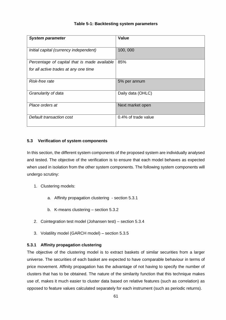
61
Table 5-1: Backtesting system parameters
System parameter Value
Initial capital (currency independent) 100, 000
Percentage of capital that is made available
for all active trades at any one time
85%
Risk-free rate 5% per annum
Granularity of data Daily data (OHLC)
Place orders at Next market open
Default transaction cost 0.4% of trade value
5.3 Verification of system components
In this section, the different system components of the proposed system are individually analysed
and tested. The objective of the verification is to ensure that each model behaves as expected
when used in isolation from the other system components. The following system components will
undergo scrutiny:
1. Clustering models:
a. Affinity propagation clustering - section 5.3.1
b. K-means clustering – section 5.3.2
2. Cointegration test model (Johansen test) – section 5.3.4
3. Volatility model (GARCH model) – section 5.3.5
5.3.1 Affinity propagation clustering
The objective of the clustering model is to extract baskets of similar securities from a larger
universe. The securities of each basket are expected to have comparable behaviour in terms of
price movement. Affinity propagation has the advantage of not having to specify the number of
clusters that has to be obtained. The nature of the similarity function that this technique makes
use of, makes it much easier to cluster data based on relative features (such as correlation) as
opposed to feature values calculated separately for each instrument (such as periodic returns).

62
As described in section 4.2, feature extraction is done over a one-year moving period in order to
resemble the parameters chosen in the study by Gatev et al [6]. In order to test the functionality
of the affinity propagation clustering model, stocks listed on the Deutsche Börse Xetra were
examined over the period January 2004 – January 2005 (approximately 252 trading days). The
securities were clustered with a similarity function based on the correlation and squared-error
between the normalized price series of the securities (see section 4.2.2).
Table 5-2 displays the clusters that were formed. The first column contains a generic cluster
number that does not hold any significant meaning. The ticker symbols of the securities that
belong to the cluster are displayed in the second column with the respective sectors that these
securities belong to listed in the third column.
In the case of a cluster containing only one security, the respective security is placed in the same
group as the security which has the lowest squared-error when compared with the single security.
Since the Johansen test can only test for cointegration for time series up to a maximum of twelve,
clusters that contain more than twelve securities are split in half until all clusters have a size: 2 ≤
𝑛 ≤ 12. These changes are not shown in Table 5-2.
From Table 5-2 it is clear that most clusters contain a blend of different sectors. Only cluster 2
and cluster 9 were clearly dominated by a certain industry. Cluster 2 contained only companies
from the automobile/manufacturing sector and cluster 9 contained mostly pharmaceutical
companies. It should be noted that the objective of the clustering model is not to explain why
certain securities are related, but only to suggest which securities had comparable movements in
the past year.
The price series of cluster 1 and cluster 2 are displayed in Figure 5-1 and Figure 5-2 respectively.
From these figures it is clear that the securities in each cluster had similar movements in the
period that is investigated. The price series in these figures are normalized and adjusted for
dividends and splits.

63
Table 5-2: Clustering of German stocks (2004-2005) - AP
Cluster
#
Ticker symbols that belong to cluster Sectors contained in cluster
1 alv.de, gbf.de, mlp.de, sie.de, vow3.de Insurance, Industrial, Financial,
Automobile
2 bmw.de, dai.de, man.de Automobile, Manufacturing
3 sgl.de, tka.de, pwn.de, hbm.de, bayn.de,
hot.de, dte.de, cbk.de
Chemicals, Industrial, Retail,
Construction, Telecommunication,
Banks
4 sur.de, ttk.de, rwe.de, bas.de, rsl2.de,
hei.de, fpe3.de, sdf.de, lin.de, ads.de,
nda.de, acwn.de, rhk.de, ku2.de, con.de,
szg.de, eoan.de
Basic resources, Retail, Utilities,
Chemicals, Industrial, Construction,
Consumer, Health Care, Automobile
5 haw.de Retail
6 hen3.de, hen.de, gfk.de, dbk.de, inh.de,
szu.de
Consumer, Industrial, Banks, Food
& Beverages
7 eck.de, bei.de, jun3.de, lei.de, drw3.de,
due.de, g1a.de, dam.de
Retail, Consumer, Industrial,
Pharma & Healthcare, Technology
8 gil.de, muv2.de, saz.de, dez.de, lha.de,
vow.de, hdd.de, use.de, six2.de, vos.de
Industrial, Insurance, Pharma &
Healthcare, Transportation &
Logistics, Automobile,
9 fme.de, srt.de, bio3.de, bio.de, meo.de,
mrk.de, pum.de
Pharma & Healthcare, Retail,
Consumer
10 sap.de Software

64
Figure 5-1: Price series from DE cluster 1
Figure 5-2: Price series from DE cluster 2

65
5.3.2 K-means clustering
K-means clustering was developed as a method of vector quantization for usage in cluster
analysis. The implementation details of this model are discussed in section 4.4.1. As described
in section 4.2, feature extraction is done over a one-year moving period. In order to test the
functionality of the k-means clustering model, stocks listed on the Deutsche Börse Xetra were
examined over the period January 2004 – January 2005 (approximately 252 trading days).
As a method of testing the k-means clustering model, the absolute returns over small periods
were used as the features of the price series. Since 252 trading days are observed and a month
has generally 22 trading days, the absolute return of each month is used as a feature. The
reasoning for this approach is that similar securities should have similar returns throughout the
year. The number of clusters to be formed was chosen as 𝑘 = 10 to allow for comparison with the
results of the affinity propagation technique in section 5.3.1.
The results of the k-means clustering on stocks listed on the Deutsche Börse Xetra over the period
January 2004 – January 2005 can be seen in Table 5-3. As with the clusters formed using the
affinity propagation technique, each cluster contains a blend of securities from different sectors.
The software company SAP SE O.N. was extracted to its own cluster, similar to that of the results
in Table 5-2. The automobile and manufacturing companies BMW, DAI and MAN were also found
in the same cluster. A number of other noticeable similarities are present in the clusters formed
by the affinity propagation technique and the clusters formed by the k-means technique. A further
investigation into the suitability of these clusters for statistical arbitrage is performed in section
5.3.3.

66
Table 5-3: Clustering of German stocks (2004-2005) – k-means
Cluster Ticker symbols that belong to cluster Sectors contained in cluster
1 eck.de, hen.de, lha.de, man.de, rsl2.de,
saz.de, srt.de, szg.de
Retail, Consumer, Transportation &
Logistics, Industrial, Basic
resources, Pharmaceuticals &
Healthcare
2 ads.de, bei.de, gbf.de, haw.de, hdd.de,
hei.de, mrk.de, sgl.de, sur.de, szu.de,
use.de, acwn.de
Consumer, Industrial, Retail,
Construction, Pharmaceuticals &
Healthcare, Chemicals, Basic
resources, Food & Beverages
3 sap.de Software
4 cbk.de, eoan.de, lin.de, rwe.de, skb.de,
vos.de
Banks, Utilities, Chemicals,
Industrial
5 bayn.de, due.de, fme.de, gfk.de, hbm.de,
hen3.de, inh.de, ku2.de, lei.de, meo.de,
sap.de, tka.de
Chemicals, Industrial,
Pharmaceuticals & Healthcare,
Retail, Consumer, Software
6 bas.de, con.de, dam.de, dez.de, dte.de,
fpe3.de, gil.de, mlp.de, nda.de, pwo.de,
rhk.de, sdf.de, six2.de, ttk.de
Chemicals, Automobile,
Technology, Industrial,
Telecommunication, Financial
service, Basic resources,
Transportation and Logistics, Retail
7 dbk.de, sie.de Banks, Industrial
8 bmw.de, dai.de, man.de Automobile, Manufacturing
9 bio3.de, dai.de, hot.de, jun3.de, vow.de,
vow3.de, pum.de, bio.de
Pharmaceuticals & Healthcare,
Automobile, Construction, Industrial
10 alv.de, g1a.de, muv2.de, drw3.de Insurance, Industrial,
Pharmaceuticals & Healthcare

67
5.3.3 Comparison of clustering techniques
The comparison of clustering techniques (in general) can be a processing intensive and difficult
task due to the inherent characteristic of many data sets where an optimal cluster set is not
necessarily known. In order to simplify the comparison for the application of this study, it is firstly
assumed that a larger number of cointegrating relations is more favourable than a smaller number
of cointegrating relations. As a means of comparing k-means clustering and affinity propagation
clustering, the number of cointegrating relations found from the resulting clusters will determine
the suitability of each technique in this application.
The period of January 2005 - January 2006 is observed for the different stock markets. Affinity
propagation does not require the number of clusters to be specified, but in the case of k-means it
was chosen as 𝑘 =𝑁
5 where 𝑁 depicts the size of the universe. The choice for dividing the universe
size by 5 stems from the proposed basket size to be traded. The number of cointegrating relations
found from the resulting clusters will be counted. It is important to note that for both clustering
methods, clusters larger than 12 securities will be split with no particular order. The results can
be seen in Table 5-4.
Table 5-4: Comparison of clustering techniques based on number of cointegrating
relations
Security universe Affinity Propagation K-means
DE stocks 14 6
JP stocks 54 37
SA stocks 34 28
US stocks 58 25
From Table 5-4 it is clear that more cointegrating relations were found from the resulting clusters
for affinity propagation than for k-means clustering. The results suggest that using affinity
propagation may be more useful in this study. As with any clustering problem, it is possible to
obtain different results when other features are extracted. The main advantage of affinity
propagation in this application is that it clusters according to a similarity function and not according
to absolute values where k-means could potentially perform better.

68
As an empirical test for comparing the clustering techniques, two versions of the adaptive system
were implemented and tested on the different stock universes over the period of 2006 – 2016.
The results are summarized in Table 5-5 which displays the alpha (excess returns) produced on
each universe. The complete backtest results can be found in Appendix C.
Table 5-5: Backtest comparison of system using different clustering techniques
Security universe Affinity Propagation
(Alpha %)
K-means (Alpha %)
DE stocks 3.0512 -6.2857
JP ETFs 3.7382 1.6006
JP stocks 8.4728 2.1312
SA stocks 3.2654 1.5981
US ETFs -4.1094 -9.9870
US stocks 2.3255 -1.7942
The results that were provided in this section show that the affinity propagation clustering
technique performs significantly better than the k-means clustering approach for this application.
Hence, the version of the system that is validated in the remainder of this chapter uses the affinity
propagation technique for creating clusters of securities.
5.3.4 Johansen cointegration test
The Johansen test is used to determine whether time series are cointegrated. If a number of time
series are found to be cointegrated, a linear combination of the original time series can result in
a (weakly) stationary series. The Johansen test makes it possible to test up to twelve time series
for cointegrating relations at a time. The resulting eigenvectors from the Johansen test can be
used as linear weights that would create a stationary series.
In this section, the Johansen test will be applied to a varying number of securities. The securities
that will be tested include ETFs and stocks from different exchanges. The choice of securities that
will be tested for cointegration stems from known cointegrated series that have been documented
in previous studies, securities that are commonly believed to be similar and securities that have
been clustered together in sections 5.3.1 and 5.3.2.

69
5.3.4.1 Johansen test applied to two index funds
Two MSCI country index funds that have been frequently tested for cointegration are the Australia
index fund (EWA) and the Canada index fund (EWC). Chan [5] popularized these ETFs as
tradable using mean-reversion models, having shown that these securities are indeed
cointegrated. The price series of these funds are depicted in Figure 5-3 over a period of March
2005 to March 2006 (approximately 252 trading days).
Figure 5-3: EWA/EWC price series (2005-2006)
When the Johansen test is performed on the series, two hypothesis tests are done (as discussed
in section 4.5.6). The null hypothesis states that there are exactly 𝑟 cointegrating relations. In this
case, the largest value of the log likelihood function is given by equation (4.20). The null
hypothesis can be rejected when the test statistic is larger than a certain critical value. The
discarding of the null hypothesis is thus connected to a certain statistical significance. As an
example, if the null hypothesis of 𝑟 ≤ 0 is discarded, the test states that there is at least one
cointegrating relation that exists (with regards to a confidence level). This means that there exists
at least one set of linear weights that will form a stationary series based on the input price series.
The results of the two hypothesis tests are contained in Table 5-6 and Table 5-7.

70
Table 5-6: Trace test results (EWA/EWC)
NULL: Trace statistic Crit 90% Crit 95% Crit 99%
𝑟 ≤ 0 17.5764 13.4294 15.4943 19.9349
𝑟 ≤ 1 0.0863529 2.7055 3.8415 6.6349
Table 5-7: Eigen test results (EWA/EWC)
NULL: Eigen statistic Crit 90% Crit 95% Crit 99%
𝑟 ≤ 0 17.49 12.2971 14.2639 18.52
𝑟 ≤ 1 0.0863529 2.7055 3.8415 6.6349
The trace test indicates that the null hypothesis can be discarded with a certainty level of 95%
since the trace statistic (17.5764) is larger than the 95% critical value (15.4943), but less than the
99% critical value (19.9349). The eigen test also indicates that the null hypothesis can be
discarded with a certainty level of 95% as the eigen statistic (17.49) is larger than the 95% critical
value (14.2639), but less than the 99% critical value (18.52). If the null hypothesis of 𝑟 ≤ 0 is
discarded (as is the case), the test states that there is at least one cointegrating relation that exists
(with regards to the confidence level). If the null hypothesis of 𝑟 ≤ 1 would have been discarded,
the test states that more than one cointegrating relation may exist. In this case, both hypothesis
tests suggest that only one cointegrating relation exists since the 𝑟 ≤ 1 null hypothesis could not
be discarded by any of two tests.
Since the securities EWC and EWA have been shown to be cointegrated over the examined
period, it is possible to construct a stationary portfolio using a linear combination of these
securities. The eigenvector that is associated with the largest eigenvalue from the Johansen test
results is given as:
𝑣 = [4.1434
−1.7232]
By using the eigenvector to weigh EWC with 4.1434 for every -1.7232 that EWA is weighed, the
series in Figure 5-4 is obtained.

71
Figure 5-4: Stationary series from EWA/EWC
5.3.4.2 Johansen test applied to two US stocks during the 2008 crash
As in section 5.3.4.2, the Johansen test will again be applied to only two securities. In this case,
the stock prices of two NYSE listed stocks (that compete in the same industry) will be tested for
cointegration. MasterCard (ma.us) has been listed on the NYSE since May 2006 and Visa (v.us)
has been listed since March 2008. These companies compete in the financial services industry
as primary suppliers of bank cards.
The Johansen test will be done for a period of one year since Visa was listed on the NYSE. This
period is of significance since it includes the financial crash of 2008. The stock prices over this
period is displayed in Figure 5-5.
Table 5-8: Trace test results (MA/V)
NULL: Trace statistic Crit 90% Crit 95% Crit 99%
𝑟 ≤ 0 18.724 13.4294 15.4943 19.9349
𝑟 ≤ 1 0.829024 2.7055 3.8415 6.6349
Table 5-9: Eigen test results (MA/V)
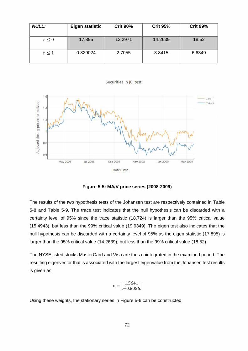
72
NULL: Eigen statistic Crit 90% Crit 95% Crit 99%
𝑟 ≤ 0 17.895 12.2971 14.2639 18.52
𝑟 ≤ 1 0.829024 2.7055 3.8415 6.6349
Figure 5-5: MA/V price series (2008-2009)
The results of the two hypothesis tests of the Johansen test are respectively contained in Table
5-8 and Table 5-9. The trace test indicates that the null hypothesis can be discarded with a
certainty level of 95% since the trace statistic (18.724) is larger than the 95% critical value
(15.4943), but less than the 99% critical value (19.9349). The eigen test also indicates that the
null hypothesis can be discarded with a certainty level of 95% as the eigen statistic (17.895) is
larger than the 95% critical value (14.2639), but less than the 99% critical value (18.52).
The NYSE listed stocks MasterCard and Visa are thus cointegrated in the examined period. The
resulting eigenvector that is associated with the largest eigenvalue from the Johansen test results
is given as:
𝑣 = [1.5641
−0.8056]
Using these weights, the stationary series in Figure 5-6 can be constructed.

73
Figure 5-6: Stationary series from MA/V
5.3.4.3 Johansen test applied to US stocks in the same industry
In this section the Johansen test is applied to The Coca-Cola Co (ko.us) and PepsiCo (pep.us),
two of the largest soft drink manufacturers in the US. As in section 5.3.4.2, it may be expected
that an underlying economic relation could exist.
The Coca-Cola Co and PepsiCo have existed since the 1970s. A year that did not consist of any
major bullish market movement is examined in this section (January 2004 – January 2005). The
stock prices of these stocks are displayed in Figure 5-7. The results of the Johansen test applied
to the time series of these securities are shown in Table 5-10 and Table 5-11. Since both the
trace statistic and the eigen statistic are less than all of the critical values in these tables, the null
hypothesis that there exists 0 cointegrating vectors cannot be discarded. A stationary series can
therefore not be constructed for these securities over the examined period.

74
Figure 5-7: KO/PEP price series (2004-2005)
Table 5-10: Trace test results (KO/PEP)
NULL: Trace statistic Crit 90% Crit 95% Crit 99%
𝑟 ≤ 0 5.83009 13.4294 15.4943 19.9349
𝑟 ≤ 1 0.780517 2.7055 3.8415 6.6349
Table 5-11: Eigen test results (KO/PEP)
NULL: Eigen statistic Crit 90% Crit 95% Crit 99%
𝑟 ≤ 0 5.04957 12.2971 14.2639 18.52
𝑟 ≤ 1 0.780517 2.7055 3.8415 6.6349
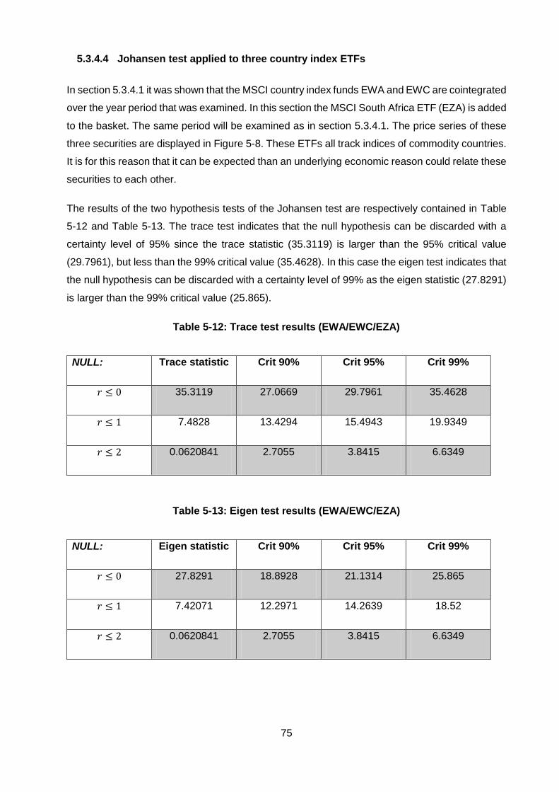
75
5.3.4.4 Johansen test applied to three country index ETFs
In section 5.3.4.1 it was shown that the MSCI country index funds EWA and EWC are cointegrated
over the year period that was examined. In this section the MSCI South Africa ETF (EZA) is added
to the basket. The same period will be examined as in section 5.3.4.1. The price series of these
three securities are displayed in Figure 5-8. These ETFs all track indices of commodity countries.
It is for this reason that it can be expected than an underlying economic reason could relate these
securities to each other.
The results of the two hypothesis tests of the Johansen test are respectively contained in Table
5-12 and Table 5-13. The trace test indicates that the null hypothesis can be discarded with a
certainty level of 95% since the trace statistic (35.3119) is larger than the 95% critical value
(29.7961), but less than the 99% critical value (35.4628). In this case the eigen test indicates that
the null hypothesis can be discarded with a certainty level of 99% as the eigen statistic (27.8291)
is larger than the 99% critical value (25.865).
Table 5-12: Trace test results (EWA/EWC/EZA)
NULL: Trace statistic Crit 90% Crit 95% Crit 99%
𝑟 ≤ 0 35.3119 27.0669 29.7961 35.4628
𝑟 ≤ 1 7.4828 13.4294 15.4943 19.9349
𝑟 ≤ 2 0.0620841 2.7055 3.8415 6.6349
Table 5-13: Eigen test results (EWA/EWC/EZA)
NULL: Eigen statistic Crit 90% Crit 95% Crit 99%
𝑟 ≤ 0 27.8291 18.8928 21.1314 25.865
𝑟 ≤ 1 7.42071 12.2971 14.2639 18.52
𝑟 ≤ 2 0.0620841 2.7055 3.8415 6.6349

76
The country index exchange-traded funds EWC, EWA and EZA are thus cointegrated in the
examined period. The resulting eigenvector that is associated with the largest eigenvalue from
the Johansen test results is given as:
𝑣 = [−3.98192.7377
−0.3200]
Using these weights, the stationary series in Figure 5-9 can be constructed.
Figure 5-8: EWA/EWC/EZA price series (2005-2006)

77
Figure 5-9: Stationary series from EWA/EWC/EZA
5.3.4.5 Johansen test applied to clustered German stocks
In section 5.3.1, affinity propagation clustering was performed on a universe of liquid stocks that
are listed on the Deutsche Börse Xetra. In this section the Johansen test is performed on one of
the resulting clusters. The cluster consists of three manufacturing stocks: Bay. Motoren Werke
(bmw.de), Daimler AG (dai.de) and MAN SE ST (man.de). The stock prices are displayed in
Figure 5-2.
Table 5-14 and Table 5-15 contain the results of the Johansen test. Since the trace statistics
(36.9122) is larger than the 99% critical value (35.4628) and the eigen statistic (21.6079) is larger
than the 90% critical value (18.8928) the null hypothesis of r ≤ 0 can be rejected. The trace test
also rejects the hypothesis that r ≤ 1, but since the eigen test does not confirm this, we cannot
reject the r ≤ 1 hypothesis.
Table 5-14: Trace test results on German stocks
NULL: Trace statistic Crit 90% Crit 95% Crit 99%
𝑟 ≤ 0 36.9122 27.0669 29.7961 35.4628
𝑟 ≤ 1 15.3043 13.4294 15.4943 19.9349
𝑟 ≤ 2 1.31548 2.7055 3.8415 6.6349

78
Table 5-15: Eigen test results on German stocks
NULL: Eigen statistic Crit 90% Crit 95% Crit 99%
𝑟 ≤ 0 21.6079 18.8928 21.1314 25.865
𝑟 ≤ 1 9.10716 12.2971 14.2639 18.52
𝑟 ≤ 2 1.31548 2.7055 3.8415 6.6349
The stationary series in Figure 5-10 can be constructed by applying the weights from the resulting
eigenvector of the Johansen test:
𝑣 = [−0.57220.10721.0536
]
Figure 5-10: Stationary series from German stocks
5.3.5 GARCH volatility model
GARCH models are used to forecast the volatility (𝜎𝑡) of a time series when there is reason to
believe that the volatility does not stay constant over time, but clusters. In this study, GARCH
models will be used to predict the volatility of the price series that have been formed by the
Johansen method. If the volatility predictions have merit, it would be possible to create more
optimal trading rules than a fixed standard deviation model for mean-reversion trading. This
section contains some experiments on different universes to model the volatility of security prices.
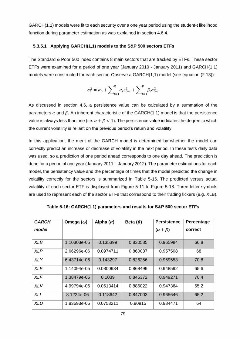
79
GARCH(1,1) models were fit to each security over a one year period using the student-t likelihood
function during parameter estimation as was explained in section 4.6.4.
5.3.5.1 Applying GARCH(1,1) models to the S&P 500 sectors ETFs
The Standard & Poor 500 index contains 8 main sectors that are tracked by ETFs. These sector
ETFs were examined for a period of one year (January 2010 - January 2011) and GARCH(1,1)
models were constructed for each sector. Observe a GARCH(1,1) model (see equation (2.13)):
𝜎𝑡2 = 𝛼0 + ∑ 𝛼𝑖휀𝑡−𝑖
2𝑞
𝑖=1+ ∑ 𝛽𝑖𝜎𝑡−𝑖
2𝑝
𝑖=1
As discussed in section 4.6, a persistence value can be calculated by a summation of the
parameters 𝛼 and 𝛽. An inherent characteristic of the GARCH(1,1) model is that the persistence
value is always less than one (i.e. 𝛼 + 𝛽 < 1). The persistence value indicates the degree to which
the current volatility is reliant on the previous period’s return and volatility.
In this application, the merit of the GARCH model is determined by whether the model can
correctly predict an increase or decrease of volatility in the next period. In these tests daily data
was used, so a prediction of one period ahead corresponds to one day ahead. The prediction is
done for a period of one year (January 2011 – January 2012). The parameter estimations for each
model, the persistency value and the percentage of times that the model predicted the change in
volatility correctly for the sectors is summarized in Table 5-16. The predicted versus actual
volatility of each sector ETF is displayed from Figure 5-11 to Figure 5-18. Three letter symbols
are used to represent each of the sector ETFs that correspond to their trading tickers (e.g. XLB).
Table 5-16: GARCH(1,1) parameters and results for S&P 500 sector ETFs
GARCH
model
Omega (𝝎) Alpha (𝜶) Beta (𝜷) Persistence
(𝜶 + 𝜷)
Percentage
correct
XLB 1.10303e-05 0.135399 0.830585 0.965984 66.8
XLP 2.66296e-06 0.0974711 0.860037 0.957508 68
XLY 6.43714e-06 0.143297 0.826256 0.969553 70.8
XLE 1.14094e-05 0.0800934 0.868499 0.948592 65.6
XLF 1.38479e-05 0.1039 0.845372 0.949271 70.4
XLV 4.99794e-06 0.0613414 0.886022 0.947364 65.2
XLI 8.1224e-06 0.118642 0.847003 0.965646 65.2
XLU 1.83693e-06 0.0753211 0.90915 0.984471 64
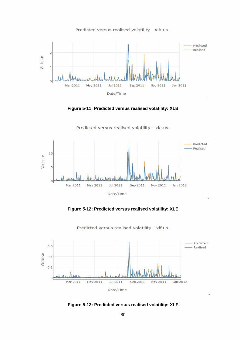
80
Figure 5-11: Predicted versus realised volatility: XLB
Figure 5-12: Predicted versus realised volatility: XLE
Figure 5-13: Predicted versus realised volatility: XLF

81
Figure 5-14: Predicted versus realised volatility: XLI
Figure 5-15: Predicted versus realised volatility: XLP
Figure 5-16: Predicted versus realised volatility: XLU

82
Figure 5-17: Predicted versus realised volatility: XLV
Figure 5-18: Predicted versus realised volatility: XLY
In order to illustrate the “prediction accuracy” of the GARCH(1,1) models on each sector ETF, a
graph was constructed that tracks the percentage of correct predictions in volatility change. Figure
5-19 shows how these values changed over the period of one year. It is interesting to note that
for all of the ETFs the “prediction accuracy” converged to just above 60%. This indicates that a
significant amount of volatility changes can be explained by the conditional heteroskedasticity.

83
Figure 5-19: Convergence of GARCH prediction accuracy
5.3.5.2 Applying GARCH(1,1) models to the MSCI country index ETFs
As an additional study of the GARCH(1,1) model applied to financial time series, the relationship
between “prediction accuracy” and the persistence value was investigated. The MSCI country
index ETFs were selected for constructing GARCH(1,1) models over the period of January 2010
to January 2011 (approximately 252 trading days). The models were used for one period
predictions over the period January 2011 to January 2012. As in section 5.3.5.1, the prediction
accuracy is once again defined as the percentage of times that the model correctly predicts an
increase or decrease in volatility. Figure 5-20 depicts a scatter plot of the findings that show that
there is no strong correlation between the values when the persistence values are above 0.9. The
Pearson correlation coefficient of the data points in Figure 5-20 is -0.188. When a GARCH model
cannot be fit to the model, it is possible for the simplex search algorithm to estimate parameters
such that the persistence value is less than 0.9. In such cases, the GARCH model will be very
unreliable in making predictions of future volatility.

84
Figure 5-20: Correct predictions versus persistence (GARCH)
The daily parameters of the GARCH model that were calculated in Table 5-16 and the parameter
values for the test on the MSCI country index ETFs lie within the normal ranges (as described in
[57]). For daily data the parameter α (GARCH reaction) ranges between 0.05 (market with
relatively low volatility) and 0.1 (market that experiences high volatility). The results are
comparable to that of Alexander [57] who showed that the persistence value generally ranges
from 0.85 to 0.98 with lower values being associated with higher α values. Figure 5-20 indicates
that prediction accuracy does not improve for higher persistence values. No persistence values
below 0.9 were found in the S&P 500 index ETFs test and MSCI country index ETFs test.
Persistence values below 0.9 are often present in GARCH models that are fitted to stocks.
5.3.5.3 GARCH-updated entry threshold versus fixed entry thresholds
As was mentioned in section 4.2.2, the use of GARCH models in this study is to dynamically
update the market entry threshold for trading the weakly stationary series obtained from linearly
weighting a group of securities. The objective of this approach is to create a more optimal set of
trading rules than using fixed deviation thresholds. A problem that arises when selecting a fixed
threshold for market entry is that an optimal value is not known a priori. By using an adaptive
threshold, the value for market entry scales with the historic and predicted volatility of the price
series. An advantage that arises from this approach is that each basket that is traded has its own
model for timing market entry.

85
As a means of comparing the GARCH-updated and fixed deviation thresholds, the period of 2010-
2016 was examined for stock exchanges in Germany, South Africa and North America. Three
fixed deviation threshold versions of the system were implemented with entry values of 1.0, 1.5
and 2.0 standard deviations for comparison with the GARCH-updated model that was described
in section 4.2.2. The complete backtest results can be seen in Appendix D.
The first set of results for the German stock exchange is depicted in Figure 5-21. In this case, the
dynamically updated threshold proved to provide better returns, but with larger drawdown, than
the fixed deviation systems. The 2.0 standard deviation system obtained the best results of the
three fixed systems.
In the case of the South African stock exchange (Figure 5-22), the adaptive system had the
second best returns and the highest drawdown. The highest compound annual growth rate was
obtained by the 2.0 standard deviation system. The backtest on the US stock markets is shown
in Figure 5-23. In this case the adaptive system had the second best returns with comparable
drawdown to the 1.0 standard deviation system which had the best compound annual growth rate.
From these results it is clear that the GARCH-updated threshold for market entry does not
consistently beat the best fixed standard deviation systems. It does have some merit in that the
compound annual growth rate was always in the top two of the systems examined, but it does not
improve on drawdown experienced.
Figure 5-21: Varying versus fixed entry thresholds (DAX)
0
5
10
15
1.0 SDSystem
1.5 SDSystem
2.0 SDSystem
AdaptiveSystem (1.0)
CAGR
-0.2
0
0.2
0.4
0.6
1.0 SDSystem
1.5 SDSystem
2.0 SDSystem
AdaptiveSystem (1.0)
Sharpe
0
5
10
15
20
1.0 SDSystem
1.5 SDSystem
2.0 SDSystem
AdaptiveSystem (1.0)
Max Drawdown
-0.5
0
0.5
1
1.5
1.0 SDSystem
1.5 SDSystem
2.0 SDSystem
AdaptiveSystem (1.0)
Sortino

86
Figure 5-22: Varying versus fixed entry thresholds (JSE)
Figure 5-23: Varying versus fixed entry thresholds (US)
0
2
4
6
8
1.0 SDSystem
1.5 SDSystem
2.0 SDSystem
AdaptiveSystem (1.0)
CAGR
-0.2
-0.1
0
0.1
0.2
1.0 SDSystem
1.5 SDSystem
2.0 SDSystem
AdaptiveSystem
(1.0)
Sharpe
0
2
4
6
8
10
12
14
1.0 SDSystem
1.5 SDSystem
2.0 SDSystem
AdaptiveSystem (1.0)
Max Drawdown
-0.6
-0.4
-0.2
0
0.2
0.4
1.0 SDSystem
1.5 SDSystem
2.0 SDSystem
AdaptiveSystem (1.0)
Sortino
0
2
4
6
8
10
1.0 SDSystem
1.5 SDSystem
2.0 SDSystem
AdaptiveSystem (1.0)
CAGR
-0.4
-0.2
0
0.2
0.4
0.6
1.0 SDSystem
1.5 SDSystem
2.0 SDSystem
AdaptiveSystem (1.0)
Sharpe
0
2
4
6
8
10
1.0 SDSystem
1.5 SDSystem
2.0 SDSystem
AdaptiveSystem (1.0)
Max Drawdown
-0.5
0
0.5
1
1.5
1.0 SDSystem
1.5 SDSystem
2.0 SDSystem
AdaptiveSystem (1.0)
Sortino

87
In Appendix F, different versions of the GARCH-updated entry thresholds are examined. The
results indicate that the GARCH-updated models can provide better performance than the fixed
deviation thresholds provided that the initial deviations thresholds are optimized.
5.4 Validation of system
In this section, the proposed system is compared to the pairs trading strategy that was proposed
by Gatev et al [6] and to a stock index that tracks the market of each respective country from
which the securities were selected. Both the pairs trading strategy and the proposed system is
configured according to the default parameters that were listed in section 4.2.1 and section 4.2.2.
The objective of this validation phase is to illustrate the performance of the system under default
parameters. The sensitivity analysis in section 5.4.8 indicates the performance under a sweep of
different parameter values. The benchmark indices are listed in Table 5-17.
Table 5-17: Chosen benchmarks for validation
Country Benchmark index
Germany DAX index
Japan Nikkei 225 index
South Africa JSE index as tracked by MSCI fund (EZA)
United States S&P 500 index

88
5.4.1 Evaluation on Deutsche Börse Xetra
Figure 5-24: System performance on DAX stocks
Table 5-18: Performance metrics summary (DAX stocks)
Performance metric Adaptive system Pairs portfolio DAX Index
CAGR 9.0051% 5.4427% 5.9478%
Sharpe ratio 0.3233 0.0711 0.1464
Sortino ratio 0.5939 0.1186 0.2965
Maximum drawdown 39.8486% 24.4430% 54.5822%
Maximum drawdown
duration
1503 days 802 days 1476 days
Information ratio (DAX) 0.0697 -0.1760 -
Alpha (DAX) 3.0512% -0.5112% -
Beta (DAX) 0.0235 0.0067 -
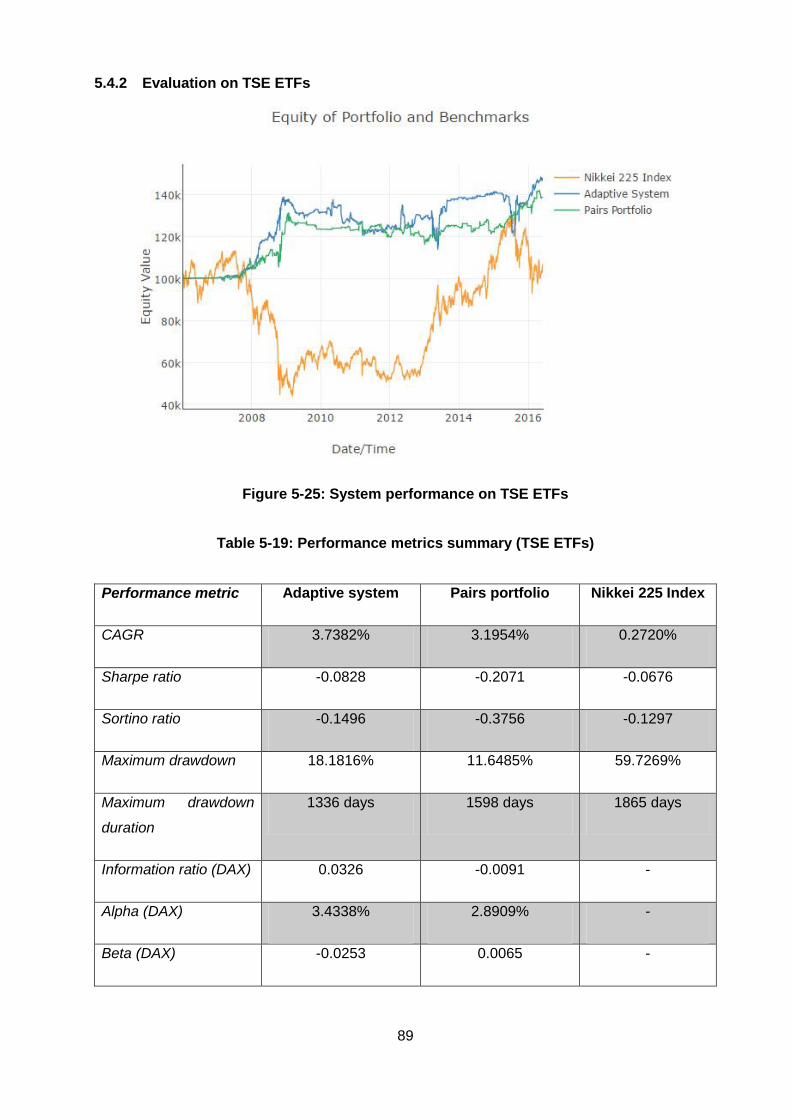
89
5.4.2 Evaluation on TSE ETFs
Figure 5-25: System performance on TSE ETFs
Table 5-19: Performance metrics summary (TSE ETFs)
Performance metric Adaptive system Pairs portfolio Nikkei 225 Index
CAGR 3.7382% 3.1954% 0.2720%
Sharpe ratio -0.0828 -0.2071 -0.0676
Sortino ratio -0.1496 -0.3756 -0.1297
Maximum drawdown 18.1816% 11.6485% 59.7269%
Maximum drawdown
duration
1336 days 1598 days 1865 days
Information ratio (DAX) 0.0326 -0.0091 -
Alpha (DAX) 3.4338% 2.8909% -
Beta (DAX) -0.0253 0.0065 -
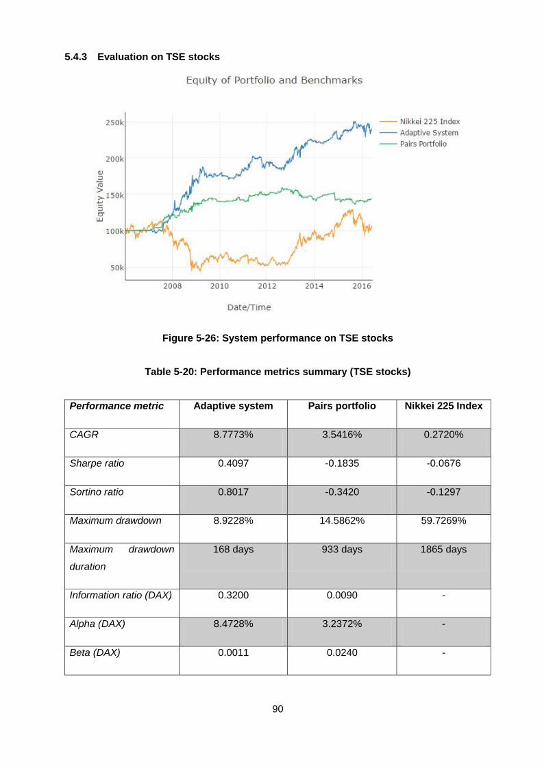
90
5.4.3 Evaluation on TSE stocks
Figure 5-26: System performance on TSE stocks
Table 5-20: Performance metrics summary (TSE stocks)
Performance metric Adaptive system Pairs portfolio Nikkei 225 Index
CAGR 8.7773% 3.5416% 0.2720%
Sharpe ratio 0.4097 -0.1835 -0.0676
Sortino ratio 0.8017 -0.3420 -0.1297
Maximum drawdown 8.9228% 14.5862% 59.7269%
Maximum drawdown
duration
168 days 933 days 1865 days
Information ratio (DAX) 0.3200 0.0090 -
Alpha (DAX) 8.4728% 3.2372% -
Beta (DAX) 0.0011 0.0240 -
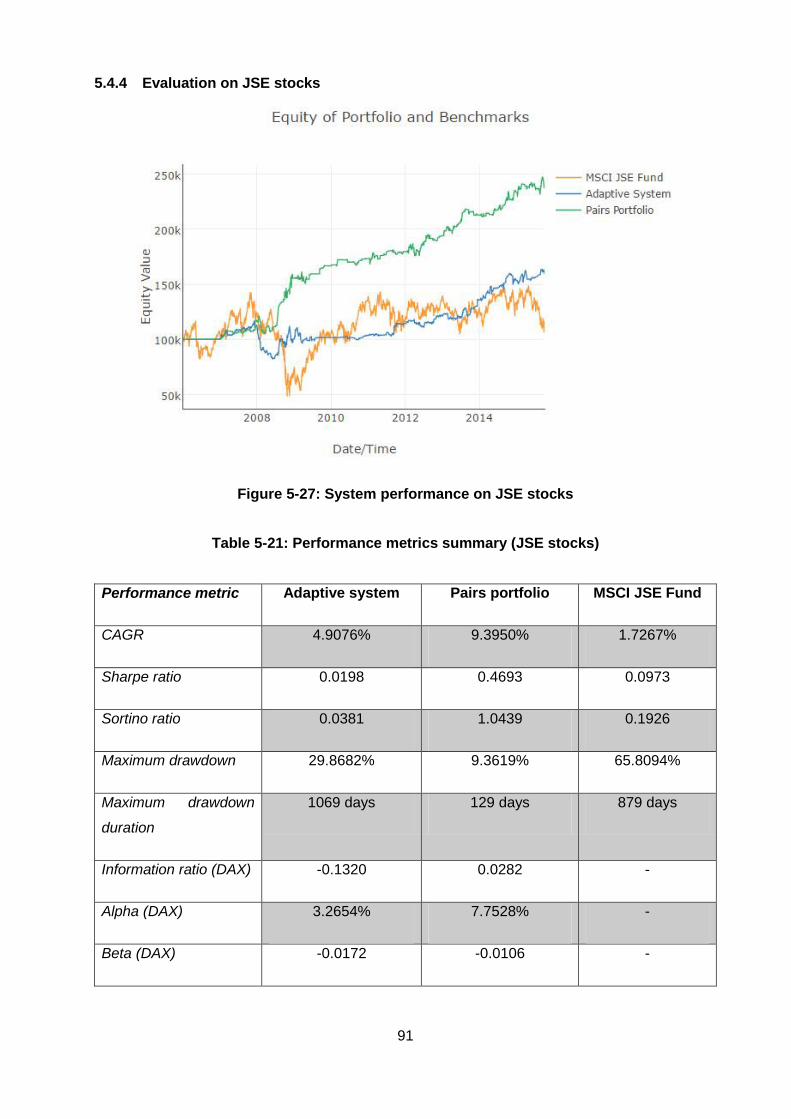
91
5.4.4 Evaluation on JSE stocks
Figure 5-27: System performance on JSE stocks
Table 5-21: Performance metrics summary (JSE stocks)
Performance metric Adaptive system Pairs portfolio MSCI JSE Fund
CAGR 4.9076% 9.3950% 1.7267%
Sharpe ratio 0.0198 0.4693 0.0973
Sortino ratio 0.0381 1.0439 0.1926
Maximum drawdown 29.8682% 9.3619% 65.8094%
Maximum drawdown
duration
1069 days 129 days 879 days
Information ratio (DAX) -0.1320 0.0282 -
Alpha (DAX) 3.2654% 7.7528% -
Beta (DAX) -0.0172 -0.0106 -

92
5.4.5 Evaluation on US ETFs
Figure 5-28: System performance on US ETFs
Table 5-22: System performance on US ETFs
Performance metric Adaptive system Pairs portfolio S&P 500 Index
CAGR 7.8518% 5.4197% 11.8893%
Sharpe ratio 0.3945 0.0825 0.4419
Sortino ratio 0.8136 0.1798 0.8594
Maximum drawdown 7.6237% 7.7455% 14.1098%
Maximum drawdown
duration
106 days 96 days 261 days
Information ratio (DAX) -0.3142 -0.4812 -
Alpha (DAX) -4.1094% -6.5415% -
Beta (DAX) 0.0138 0.0099 -
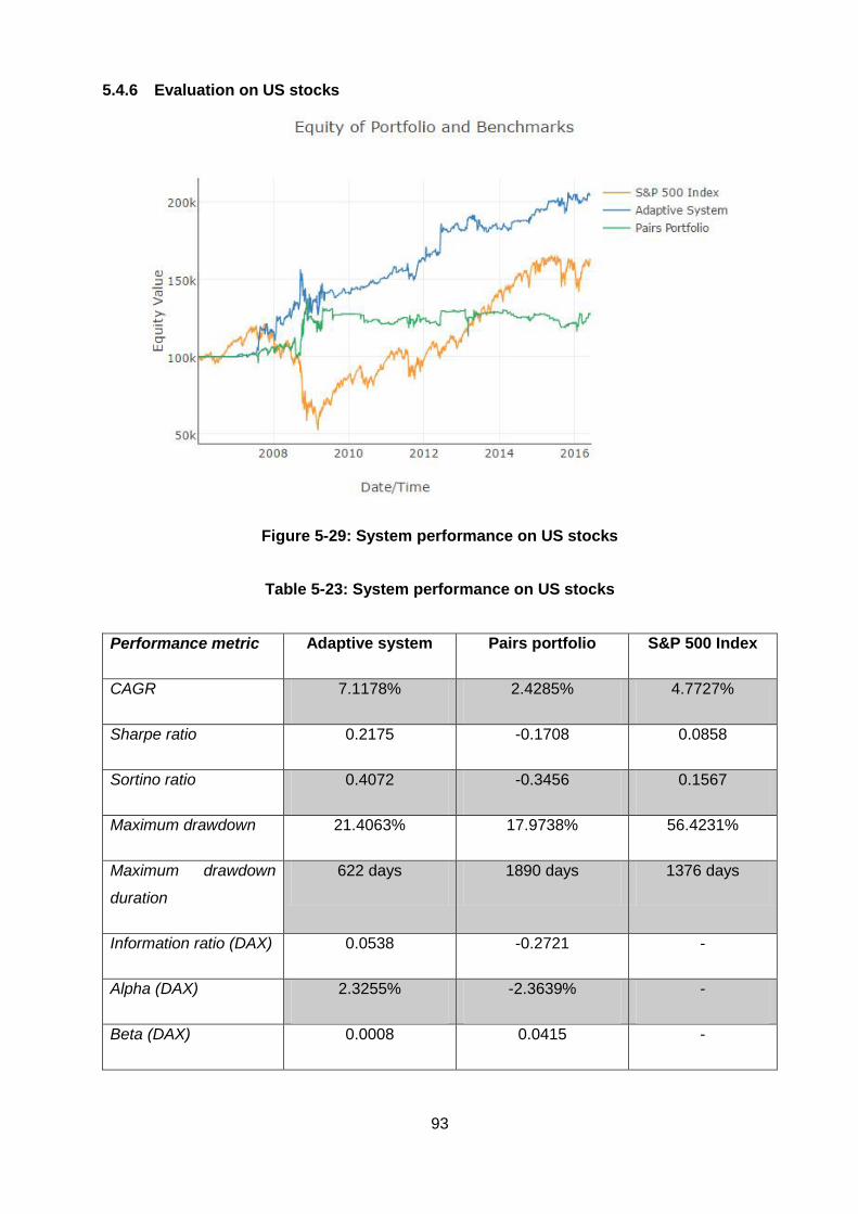
93
5.4.6 Evaluation on US stocks
Figure 5-29: System performance on US stocks
Table 5-23: System performance on US stocks
Performance metric Adaptive system Pairs portfolio S&P 500 Index
CAGR 7.1178% 2.4285% 4.7727%
Sharpe ratio 0.2175 -0.1708 0.0858
Sortino ratio 0.4072 -0.3456 0.1567
Maximum drawdown 21.4063% 17.9738% 56.4231%
Maximum drawdown
duration
622 days 1890 days 1376 days
Information ratio (DAX) 0.0538 -0.2721 -
Alpha (DAX) 2.3255% -2.3639% -
Beta (DAX) 0.0008 0.0415 -

94
5.4.7 Evaluation over different market regimes
As an additional examination of the adaptive system, a performance evaluation was performed
over two distinct periods on the US stock market. The first was the non-trending period between
2001 and 2004. During this time the S&P 500 index had a growth rate of -3.14% per year, making
it slightly bearish. The second period is the trending phase (bull market) between 2010 and 2015
when the S&P 500 index had a growth of 16.33% per year. The adaptive system and pairs trading
system were implemented using their default parameters as discussed in section 4.2. A second
version of the adaptive system (that trades up to 8 baskets of securities) was also implemented
for comparison.
A classical Bollinger bands strategy (as described by Radge [58]) was also studied during these
two distinct periods. This comparison was added to determine if the adaptive system can
outperform a much more basic approach that is also based on the concept of mean reversion.
The Bollinger bands strategy was set up to enter positions and +/- 3 standard deviations from a
simple moving average of 100 days and exit positions at +/- 1 standard deviations. The strategy
was limited to only entering 6 positions at a time. Additionally, when more than 6 trade signals
were generated at an instance, the strategy selected the 6 securities with the lowest Hurst
exponent. A low Hurst exponent (less than 0.5) indicates a high level of mean reversion.
The results of this performance evaluation can be seen in Figure 5-30 for the non-trending period
and in Figure 5-31 for the trending period. The two versions of the adaptive system, the pairs
trading system and the Bollinger Bands strategy were able to outperform the S&P 500 index
during the non-trending period, having alphas of 11.81%, 12.23%, 9.21% and 2.72% respectively.
The Bollinger Bands strategy experienced the most volatility during this period and did not have
a positive return over this period.
During the trending period, the S&P 500 index performed better than the mean-reversion
strategies. The adaptive system with default parameters had a comparable volatility to the index
and an alpha of -2.58%. The version of the adaptive system that trades up to eight baskets, had
less volatility than the index and had an alpha of -0.78%. The pairs trading strategy had very low
volatility and delivered an alpha of -8.71%, The Bollinger Bands strategy had the highest volatility
and an alpha of -31.39%.
The results indicate that the mean-reversion strategies perform better in non-trending periods
than in trending periods. The strategies were not able to outperform the index in the upward
trending market regime that was examined. The Bollinger bands strategy proved to have very
little predictive power during both of the periods that were investigated.

95
Figure 5-30: Non-trending market performance comparison
Figure 5-31: Trending market performance comparison

96
5.4.8 Sensitivity analysis
In finance and engineering, sensitivity analyses are used to understand the impact of different
parameter values on the performance of a system or model and to determine an acceptable range
of values over which these parameters may be allowed to vary without significantly degrading
system performance. A sensitivity analysis on the adaptive system will be performed for all of the
financial markets that are examined in this study. The sensitivity analysis will be done by
performing a series of one-at-a-time (OAT/ OFAT) tests. The process can be summarized as
follows [59]:
1. Move one of the system parameters, while keeping the others parameters at their default
(baseline) values as chosen in section 4.2
2. Return the changed parameter to its default value and repeat step 1 for the next system
parameter
The performance metrics chosen for observation during the sensitivity analysis include the
compound annual growth rate (CAGR), the Sharpe ratio and the Sortino ratio. As was explained
in section 4.7, the Sharpe ratio measures the risk-adjusted performance of a trading system where
risk is measured by volatility (or variance). The Sortino ratio also measures the risk-adjusted
performance of a trading system, but differs in that risk is calculated as only downside deviation.
It can thus be expected that the magnitude of the Sortino ratio will be higher than the magnitude
of the Sharpe ratio. The parameter sweep values are shown in Table 5-24. These parameters are
the only selectable parameters for the adaptive system as the thresholds for market entry are
GARCH-updated and the closing of positions take place when prices have converged (or when
the trading period ends). The results of the sensitivity analysis are summarized and charted from
section 5.4.8.1 to section 5.4.8.6.
Table 5-24: Parameter sweep ranges
Parameter Values for sweep (5) Units
Learning period 0.5 1 1.5 2 2.5 Trading years (±252 days)
Trading period 0.2 0.35 0.5 0.65 0.8 Trading years (±252 days)
Maximum number of baskets
traded at one time
2 5 8 11 14 Baskets

97
5.4.8.1 Deutsche Börse Xetra
Table 5-25: Sensitivity analysis results (DAX stocks)
Learn Period Trade Period Number of baskets CAGR Sharpe Sortino
0.5 0.5 5 8.0456 0.2598 0.4287
1 0.5 5 9.0051 0.3233 0.5939
1.5 0.5 5 6.81259 0.180537 0.307287
2 0.5 5 2.27702 -0.139715 -0.235246
2.5 0.5 5 3.95938 -0.036881 -0.0710387
Learn Period Trade Period Number of baskets CAGR Sharpe Sortino
1 0.2 5 10.5887 0.418823 0.77284
1 0.35 5 4.09359 -0.0214521 -0.0380689
1 0.5 5 9.0051 0.3233 0.5939
1 0.65 5 7.92043 0.267384 0.531055
1 0.8 5 5.68344 0.103954 0.179046
Learn Period Trade Period Number of baskets CAGR Sharpe Sortino
1 0.5 2 2.70722 -0.265681 -0.416853
1 0.5 5 9.0051 0.3233 0.5939
1 0.5 8 11.2568 0.380728 0.649459
1 0.5 11 6.20304 0.20654273 0.3568472
1 0.5 14 6.989371 0.21426872 0.4285469
AVERAGE 6.903499 0.16921389 0.3116183
Figure 5-32: Sensitivity charts (DAX stocks)
-5
0
5
100.5
1
1.52
2.5
Sensitivity of learning period
CAGR Sortino
-505
1015
0.2
0.35
0.50.65
0.8
Sensitivity of trading period
CAGR Sortino
-5
0
5
10
152
5
811
14
Sensitivity of baskets to trade
CAGR Sortino
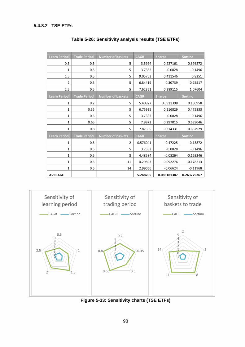
98
5.4.8.2 TSE ETFs
Table 5-26: Sensitivity analysis results (TSE ETFs)
Learn Period Trade Period Number of baskets CAGR Sharpe Sortino
0.5 0.5 5 3.5924 0.227161 0.376272
1 0.5 5 3.7382 -0.0828 -0.1496
1.5 0.5 5 9.05753 0.411546 0.8251
2 0.5 5 6.84419 0.30739 0.75517
2.5 0.5 5 7.62351 0.389115 1.07604
Learn Period Trade Period Number of baskets CAGR Sharpe Sortino
1 0.2 5 5.40927 0.0911398 0.180958
1 0.35 5 6.75935 0.216829 0.475833
1 0.5 5 3.7382 -0.0828 -0.1496
1 0.65 5 7.9972 0.297015 0.639046
1 0.8 5 7.87365 0.314331 0.682929
Learn Period Trade Period Number of baskets CAGR Sharpe Sortino
1 0.5 2 0.576041 -0.47225 -0.13872
1 0.5 5 3.7382 -0.0828 -0.1496
1 0.5 8 4.48584 -0.08264 -0.169246
1 0.5 11 4.29893 -0.092276 -0.178213
1 0.5 14 2.99056 -0.06624 -0.11968
AVERAGE 5.248205 0.086181387 0.263779267
Figure 5-33: Sensitivity charts (TSE ETFs)
-202468
100.5
1
1.52
2.5
Sensitivity of learning period
CAGR Sortino
-202468
0.2
0.35
0.50.65
0.8
Sensitivity of trading period
CAGR Sortino
-1012345
2
5
811
14
Sensitivity of baskets to trade
CAGR Sortino

99
5.4.8.3 TSE Stocks
Table 5-27: Sensitivity analysis results (TSE stocks)
Learn Period
Trade Period
Number of baskets CAGR Sharpe Sortino
0.5 0.5 5 9.20806 0.430276 0.865274
1 0.5 5 8.7773 0.4097 0.8017
1.5 0.5 5 -1.42831 -0.585819 -1.04153
2 0.5 5 -0.33109 -0.454977 -0.834837
2.5 0.5 5 1.90507 -0.301054 -0.553888
Learn Period
Trade Period
Number of baskets CAGR Sharpe Sortino
1 0.2 5 3.84395 -0.0634385 -0.124757
1 0.35 5 6.10919 0.160578 0.321744
1 0.5 5 8.7773 0.4097 0.8017
1 0.65 5 0.714476 -0.413197 -0.789351
1 0.8 5 7.6507 0.312473 0.645773
Learn Period
Trade Period
Number of baskets CAGR Sharpe Sortino
1 0.5 2 2.43569 -0.413922 -0.854552
1 0.5 5 8.7773 0.4097 0.8017
1 0.5 8 13.537 0.68468 1.3835
1 0.5 11 9.62773 0.427215 -0.836276
1 0.5 14 7.83224 0.3268761 0.7236172
AVERAGE 5.829107 0.089252707 0.087321147
Figure 5-34: Sensitivity charts (TSE stocks)
-5
0
5
100.5
1
1.52
2.5
Sensitivity of learning period
CAGR Sortino
-202468
100.2
0.35
0.50.65
0.8
Sensitivity of trading period
CAGR Sortino
-5
0
5
10
152
5
811
14
Sensitivity of baskets to trade
CAGR Sortino

100
5.4.8.4 JSE Stocks
Table 5-28: Sensitivity analysis results (JSE stocks)
Learn Period
Trade Period
Number of baskets CAGR Sharpe Sortino
0.5 0.5 5 11.1569 0.56105 1.24932
1 0.5 5 4.9076 0.0198 0.0381
1.5 0.5 5 10.9261 0.542606 1.11899
2 0.5 5 8.5037 0.382816 0.758746
2.5 0.5 5 4.12922 -0.0819734 -0.156554
Learn Period
Trade Period
Number of baskets CAGR Sharpe Sortino
1 0.2 5 -1.20224 -0.4988 -0.919437
1 0.35 5 4.31469 -0.0252368 -0.0459865
1 0.5 5 4.9076 0.0198 0.0381
1 0.65 5 9.46464 0.377095 0.785001
1 0.8 5 5.52415 0.073739 0.133055
Learn Period
Trade Period
Number of baskets CAGR Sharpe Sortino
1 0.5 2 2.71495 -0.354753 -0.686941
1 0.5 5 4.9076 0.0198 0.0381
1 0.5 8 10.4718 0.380867 0.785831
1 0.5 11 8.21095 0.328512 0.746273
1 0.5 14 7.05285 0.265572 0.61728
AVERAGE 6.399367 0.134059587 0.299991833
Figure 5-35: Sensitivity charts (JSE stocks)
-505
1015
0.5
1
1.52
2.5
Sensitivity of learning period
CAGR Sortino
-5
0
5
100.2
0.35
0.50.65
0.8
Sensitivity of trading period
CAGR Sortino
-5
0
5
10
152
5
811
14
Sensitivity of baskets to trade
CAGR Sortino
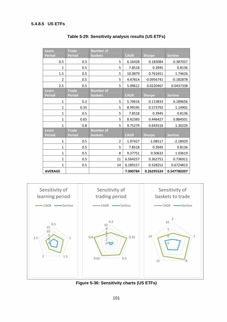
101
5.4.8.5 US ETFs
Table 5-29: Sensitivity analysis results (US ETFs)
Learn Period
Trade Period
Number of baskets CAGR Sharpe Sortino
0.5 0.5 5 6.16428 0.183084 0.387037
1 0.5 5 7.8518 0.3945 0.8136
1.5 0.5 5 10.0879 0.761651 1.74626
2 0.5 5 4.47814 -0.0956741 -0.182878
2.5 0.5 5 5.09612 0.0220467 0.0437338
Learn Period
Trade Period
Number of baskets CAGR Sharpe Sortino
1 0.2 5 5.70616 0.113833 0.189656
1 0.35 5 8.99195 0.573792 1.14901
1 0.5 5 7.8518 0.3945 0.8136
1 0.65 5 8.42383 0.446427 0.884501
1 0.8 5 9.75279 0.643516 1.30229
Learn Period
Trade Period
Number of baskets CAGR Sharpe Sortino
1 0.5 2 1.97427 -1.08517 -2.18929
1 0.5 5 7.8518 0.3945 0.8136
1 0.5 8 9.37751 0.50632 1.03619
1 0.5 11 6.564257 0.362751 0.736912
1 0.5 14 6.189157 0.328252 0.6724813
AVERAGE 7.090784 0.26295524 0.547780207
Figure 5-36: Sensitivity charts (US ETFs)
-505
1015
0.5
1
1.52
2.5
Sensitivity of learning period
CAGR Sortino
02468
100.2
0.35
0.50.65
0.8
Sensitivity of trading period
CAGR Sortino
-5
0
5
102
5
811
14
Sensitivity of baskets to trade
CAGR Sortino

102
5.4.8.6 US Stocks
Table 5-30: Sensitivity analysis results (US stocks)
Learn Period
Trade Period
Number of baskets CAGR Sharpe Sortino
0.5 0.5 5 -1.18982 -0.505485 -0.845388
1 0.5 5 7.1178 0.2175 0.4072
1.5 0.5 5 2.59259 -0.12317 -0.21145
2 0.5 5 1.23434 -0.252475 -0.428186
2.5 0.5 5 -2.8466 -0.5438 -0.8797
Learn Period
Trade Period
Number of baskets CAGR Sharpe Sortino
1 0.2 5 2.9982 -0.1367 -0.2517
1 0.35 5 6.96676 0.207913 0.42009
1 0.5 5 7.1178 0.2175 0.4072
1 0.65 5 7.27203 0.248221 0.490192
1 0.8 5 -4.19039 -0.494244 -0.752827
Learn Period
Trade Period
Number of baskets CAGR Sharpe Sortino
1 0.5 2 2.48603 -0.298424 -0.534375
1 0.5 5 7.1178 0.2175 0.4072
1 0.5 8 14.4178 0.601271 1.20533
1 0.5 11 12.9998 0.494071 0.932949
1 0.5 14 8.65627 0.315843 0.549273
AVERAGE 4.850027 0.011034733 0.061053867
Figure 5-37: Sensitivity charts (US stocks)
-5
0
5
100.5
1
1.52
2.5
Sensitivity of learning period
CAGR Sortino
-5
0
5
100.2
0.35
0.50.65
0.8
Sensitivity of trading period
CAGR Sortino
-5
0
5
10
152
5
811
14
Sensitivity of baskets to trade
CAGR Sortino
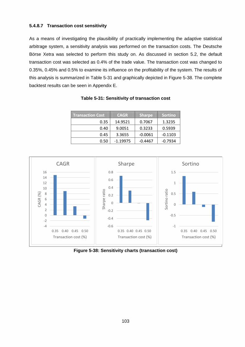
103
5.4.8.7 Transaction cost sensitivity
As a means of investigating the plausibility of practically implementing the adaptive statistical
arbitrage system, a sensitivity analysis was performed on the transaction costs. The Deutsche
Börse Xetra was selected to perform this study on. As discussed in section 5.2, the default
transaction cost was selected as 0.4% of the trade value. The transaction cost was changed to
0.35%, 0.45% and 0.5% to examine its influence on the profitability of the system. The results of
this analysis is summarized in Table 5-31 and graphically depicted in Figure 5-38. The complete
backtest results can be seen in Appendix E.
Table 5-31: Sensitivity of transaction cost
Transaction Cost CAGR Sharpe Sortino
0.35 14.9521 0.7067 1.3235
0.40 9.0051 0.3233 0.5939
0.45 3.3655 -0.0061 -0.1103
0.50 -1.19975 -0.4467 -0.7934
Figure 5-38: Sensitivity charts (transaction cost)
-4
-2
0
2
4
6
8
10
12
14
16
0.35 0.40 0.45 0.50
CA
GR
(%
)
Transaction cost (%)
CAGR
-0.6
-0.4
-0.2
0
0.2
0.4
0.6
0.8
0.35 0.40 0.45 0.50
Shar
pe
rati
o
Transaction cost (%)
Sharpe
-1
-0.5
0
0.5
1
1.5
0.35 0.40 0.45 0.50
Sort
ino
rat
io
Transaction cost (%)
Sortino
104
5.5 Review of evaluation
In this section the system design was scrutinized by evaluating each of the system components
on a number of different data sets. The complete system was tested on the different financial
markets that were selected for this research and a sensitivity analysis was performed.
The clustering techniques that were selected for the system were tested and compared. Affinity
propagation clustering proved to be better suited for this application as more cointegrating
relations were found in the resulting clusters than in those resulting from k-means clustering.
Additionally two versions of the adaptive system were implemented, the first using affinity
propagation clustering and the second using k-means clustering. The first system outperformed
the second on all of the markets tested (using the default system parameters).
The Johansen method was validated by applying it to index funds, two US stocks during the
financial crisis, US stocks that are located in the same industry, country index ETFs and German
stocks that were clustered together using the affinity propagation technique (section 5.3.1). The
results showed that (weakly) stationary series could be successfully created using this method.
The GARCH volatility model was applied to the sector ETFs of the S&P 500 index. The results
showed that the volatility model could predict an increase or decrease in volatility correctly for
more than 60% for each of the sector ETFs. GARCH(1,1) models were also applied to the MSCI
country index ETFs. The technique for using GARCH-updated thresholds for market entry was
compared to fixed standard deviation models. The results show that the default GARCH-updated
market entry threshold could not consistently outperform all of the fixed deviation models, but in
Appendix F we show that different choices of the GARCH model deviation thresholds can still
provide superior performance when compared to the fixed deviation thresholds. The GARCH-
updated models outperformed the fixed deviation methods in seven of the nine comparative
studies that were examined in Appendix F.
Finally the system was validated on the different markets and a sensitivity analysis was
performed. The system validation indicated that the adaptive system was able to generate an
average alpha of 2.74% with an average Sharpe ratio of 0.21 using the default system values.
The classical pairs trading strategy generated an average alpha of 0.74% with an average Sharpe
ratio of 0.01. The sensitivity analysis results provided an indication of the optimal parameter set
for each of the markets. Generally trading up to eight baskets at a time allowed the system to
achieve better results than trading only up to five baskets. When the maximum number of baskets
to trade was further increased (to eleven and thirteen), the performance degraded showing
evidence that the inclusion of baskets with higher variance between constituting instruments does
not necessarily improve performance. The increase of the learning period and trading period had

105
different results for the different markets, indicating that these parameters may possibly be best
chosen by performing a parameter optimization.

106
CHAPTER 6
CONCLUSION
6.1 Study overview
In this study, statistical arbitrage opportunities were investigated for financial markets in Germany,
South Africa, Japan and the United States. An adaptive algorithmic trading system was designed
and implemented based on ideas such security clustering, cointegration testing and volatility
modelling. For each of the different markets examined, the adaptive system was compared to the
performance of the respective stock market index and a classical pairs trading strategy. The time
period for validation of these models ranges from January 2006 to June 2016. This chapter
provides the concluding remarks of this study and recommendations for future research.
6.2 Concluding remarks
6.2.1 Adaptive system overview
The adaptive system that is proposed in this study consists of three main components. The first
component is a clustering model that has the objective of dividing a large security universe into a
number of smaller groups. Securities that belong to the same group should have price series that
behave similarly. Similar price movements are sought as statistical arbitrage techniques profit
from temporary relative mispricings. Affinity propagation clustering and k-means clustering were
investigated, but the prior proved to be better suited for this application as more cointegrating
relations were found in the clusters of the affinity propagation approach than in the clusters of the
k-means approach. Backtests that were performed also confirmed that the affinity propagation
clustering technique is better suited for this application.
The second component of the adaptive system is a cointegration testing model. The Johansen
method was selected for this task as the test makes it possible to search for multiple (up to twelve)
cointegrating relations at once. The cointegration test makes it possible to test whether price
series have some underlying relation with regards to a certain statistical significance. The
Johansen test also provides linear weights for creating a (weakly) stationary series from the price
series that are found to be cointegrated. The last mentioned series is then constructed from the
weights and modelled.
The third component is a volatility model that is applied to the weakly stationary series. The
purpose of this model is to predict future volatility of this weakly stationary series. A GARCH(1,1)
model was chosen for this task. The Nelder-Mead simplex search method was chosen for
estimating the parameters of the GARCH model using a student-t likelihood function. The third

107
component allows the market entry thresholds of the weakly stationary portfolio to adapt to the
volatility that is being experienced and predicted.
The adaptive system relies on a learning period in which clustering of securities is done, the
cointegration tests are performed and the volatility models are created. A trading period then
follows for trading each of the weighted security baskets that have been selected. Limits can be
placed on these periods and on the minimum number of baskets to be traded by the system at
any single time.
6.2.2 Study objectives discussion
The first chapter of this dissertation listed the four main objectives to be completed during this
study. The first objective was to classify securities using only their price data. Two clustering
techniques were implemented for this goal that made use of affinity propagation clustering and k-
means clustering. The second objective was to model the mean-reversion characteristic that are
often present in relations between financial securities. This objective was completed by using the
Johansen method to search and test for cointegration between securities. The third objective was
trade signal generation for profiting from temporary mispricings in the mean-reversion
characteristic of the fabricated series. A GARCH-updated model was constructed which could
specify market entry thresholds based on current and predicted volatility levels. The final objective
of this study was to perform a sensitivity analysis of the statistical arbitrage system. This was
completed by doing a one-at-a-time (OAT/OFAT) sensitivity analysis of the system on all of the
different markets that were examined in this study.
6.2.3 Performance discussion
The results show that the adaptive system was able to generate positive alpha for five of the six
security universes on which the system was tested over the examined period. The system was
able to outperform classical pairs trading for all markets except the Johannesburg stock
exchange. During the time period examined, the adaptive system generated an average alpha of
2.74% with an average Sharpe ratio of 0.21. The classical pairs trading strategy generated an
average alpha of 0.74% with an average Sharpe ratio of 0.01. Both approaches delivered returns
uncorrelated to the respective stock markets that were examined.
The results suggest that statistical arbitrage strategies have declined in profitability over recent
years when compared to the results of the study on pairs trading that was done by Gatev et al [6].
This phenomenon may be explained by markets that are becoming more efficient, most likely
because mispricings are being competed away by hedge funds. Observations made in this study
also suggest that statistical arbitrage strategies are extremely sensitive to transaction costs
because of the high frequency of trading that typically accompanies this type of approach.

108
The results of the sensitivity analysis provided an indication of the regions in which parameter
values should be chosen if the system is to be practically applied. It also suggests which
parameters are more sensitive for each examined market.
6.3 Recommendations for future research
The application of the adaptive system, which was proposed in this study, could be studied on
higher frequency intraday price data. Variations on simulating trade execution with the availability
of higher frequency data could provide more insight into the profitability of this approach.
This study did not include delisted securities since data for such securities were not available.
The proposed system could be tested against a more complete data set if delisted security data
is made available for research.
6.4 Closure
The objectives set in this study for an adaptive statistical arbitrage system included the
classification of securities, modelling of the mean-reversion characteristic, trade signal generation
and finally the performing of a sensitivity analysis of the system. These objectives were achieved
and successfully validated against historic market data. The adaptive system was shown to
outperform stock index benchmarks in five of the six studied security universes. The adaptive
system also outperformed classical pairs trading in most security universes that were examined.

109
BIBLIOGRAPHY
[1] N. F. Hoggson, Banking Through the Ages, New York: Dodd, Mead & Company, 1926.
[2] C. Alexander and A. Dimitriu, “The Cointegration Alpha: Enhanced Index Tracking and
Long-Short Equity Market Neutral Strategies,” 5 August 2002. [Online]. Available:
http://ssrn.com/abstract=315619. [Accessed 14 July 2015].
[3] J. Rudy, “Four Essays in Statistical Arbitrage in Equity Markets,” June 2011. [Online].
Available: http://www.harvestalpha.com/wp-content/uploads/2013/08/phd.pdf. [Accessed
14 July 2015].
[4] M. Harlacher, “Cointegration Based Statistical Arbitrage,” 13 July 2012. [Online]. Available:
https://stat.ethz.ch/research/mas_theses/2012/harlacher.pdf. [Accessed 14 July 2015].
[5] E. P. Chan, Algorithmic Trading: Winning Strategies and Their Rationale, Hoboken: John
Wiley & Sons, 2013.
[6] E. Gatev, W. Goetzmann and K. Rouwenhorst, “Pairs Trading: Performance of a Relative
Value Arbitrage Rule,” Review of Financial Studies, vol. 19, no. 3, pp. 797-827, 2006.
[7] I. Aldridge, High-Frequency Trading: A Practical Guide to Algorithmic Strategies and
Trading Systems, Wiley, 2013.
[8] T. Hendershott, C. M. Jones and A. J. Menkveldf, “Does Algorithmic Trading Improve
Liquidity?,” Journal of Finance, vol. LXVI, no. 1, pp. 1-34, 2011.
[9] W. Sharpe and G. Alexander, Investments, Englewood: Prentice Hall, 1990.
[10] E. Thorp, “A Perspective on Quantitative Finance: Models for Beating the Market,” 2003.
[Online]. Available:
http://media.wiley.com/product_data/excerpt/11/04700235/0470023511.pdf. [Accessed 12
July 2015].
[11] E. Thorp, “A Mathematician on Wall Street,” 2000. [Online]. Available:
http://www.wilmott.com/pdfs/080617_thorp.pdf. [Accessed 13 July 2015].
110
[12] W. A. Fuller, Introduction to Statistical Time Series, New York: John Wiley and Sons,
1976.
[13] D. Posada and T. R. Buckley, “Model Selection and Model Averaging in Phylogenetics:
Advantages of Akaike,” Society of Systematic Biologists, Auckland, 2004.
[14] D. Kanhneman and A. Tversky, “Intuitive Prediction: Biases and Corrective Procedures,”
Defense Advanced Research Agency, 1977.
[15] W. F. M. De Bondt and R. Thaler, “Does the Stock Market Overreact?,” The Journal of
Finance, vol. 40, pp. 793-805, 1984.
[16] A. Bhave and N. Libertini, “A Study of Short Term Mean Reversion in Equities,” September
2013. [Online]. Available: http://www.361capital.com/wp-
content/uploads/2013/10/361_Capital_Study_Short_Term_Mean_Reversion_Equities.pdf.
[Accessed 12 July 2015].
[17] F. E. Croxton, D. J. Cowden and S. Klein, Applied General Statistics, Pitman, 1968.
[18] P. I. Palmer, Essential Maths for Geoscientists: An Introduction, John Wiley & Sons, 2014.
[19] S. Theodoridis, “Probability and Stochastic Processes,” in Machine Learning: A Bayesian
and Optimization Perspective, Academic Press, 2015, pp. 9-51.
[20] J. D. Sargan and A. Bhargava, “Testing residuals from least squares regressions for being
generated by the Gaussian random walk,” Econometrica, vol. 51, no. 1, p. 153–174, 1983.
[21] R. F. Engle and C. Granger, “Co-Integration and Error Correction: Representation,
Estimation and Testing,” Econometrica, vol. 55, no. 2, pp. 251-276, 1987.
[22] B. Sjo, “Testing for Unit Roots and Cointegration,” August 2008. [Online]. Available:
https://www.iei.liu.se/nek/ekonometrisk-teori-7-5-hp-
730a07/labbar/1.233753/dfdistab7b.pdf. [Accessed 26 June 2015].
[23] S. Johansen, Likelihood-based Inference in Cointegrated Vector Autoregressive Models,
Oxford: Clarendon Press, 1995.
111
[24] J. G. Mackinnon, A. A. Haug and L. and Michelis, “Numerical Distribution Functions of
Likelihood Ratio Tests For Cointegration,” Journal of Applied Econometrics, vol. 14, pp.
563-577, 1999.
[25] B. Mandelbrot, “The variation of certain speculative prices,” J. Business, vol. 36, p. 394–
419, 1963.
[26] E. F. Fama, “The behavior of stock-market prices,” J. Business, vol. 38, p. 34–105, 1965.
[27] R. T. Baillie, T. Bollerslev and H. O. Mikkelsen, “Fractionally integrated generalized
autoregressive conditional heterskedasticity,” J. Econometrics, vol. 74, p. 3–30, 1996.
[28] R. Engle, “GARCH 101: The Use of ARCH/GARCH Models in Applied Econometrics.,”
Journal of Economic Perspectives, vol. 15, no. 4, pp. 157-168, 2001.
[29] R. F. Engle, “Autoregressive Conditional Heteroscedasticity with Estimates of Variance of
United Kingdom Inflation,” Econometrica, vol. 50, no. 4, pp. 987-1008, 1982.
[30] K. Bailey, Typologies and Taxonomies: An Introduction to Classification Techniques, 1994.
[31] J. B. MacQueen, “Some Methods for classification and Analysis of Multivariate
Observations,” in 5th Berkeley Symposium on Mathematical Statistics and Probability,
Oakland, 1967.
[32] B. J. Frey and D. Dueck, “Clustering by Passing Messages Between Data Points,”
Science, vol. 315, no. 5814, pp. 972-976, 2007.
[33] E. F. Fama, “Efficient capital markets: A review of theory and empirical work.,” The journal
of Finance, vol. 25, no. 2, pp. 383-417, 1970.
[34] B. G. Malkiel, “The efficient market hypothesis and its critics,” The Journal of Economic
Perspectives, vol. 17, no. 1, pp. 59-82, 2003.
[35] S. J. Grossman and J. E. Stiglitz, “On the impossibility of informationally efficient markets,”
The American economic review, vol. 70, no. 3, pp. 393-408, 1980.
[36] N. Jegadeesh and S. Titman, “Returns to buying winners and selling losers: Implications
for stock market efficiency,” The journal of finance, vol. XLVIII, no. 1, pp. 65-91, 1993.

112
[37] L. Chan, N. Jegadeesh and J. Lakonishok, “Momentum strategies,” The journal of finance,
vol. LI, no. 5, pp. 1681-1713, 1996.
[38] C. Dunis and R. Ho, “Cointegration Portfolios of European Equities,” January 2005.
[Online]. Available:
http://citeseerx.ist.psu.edu/viewdoc/download?doi=10.1.1.462.4725&rep=rep1&type=pdf.
[Accessed 22 August 2015].
[39] J. Nobrega and A. Oliveira, “Improving the Statistical Arbitrage Strategy in Intraday
Trading by Combining Extreme Learning Machine and Support Vector Regression with
Linear Regression Models,” in 2013 IEEE 25th International Conference on Tools with
Artificial Intelligence, Washington DC, 2013.
[40] E. F. Fama and K. R. French, “Size, value, and momentum in international stock returns,”
Journal of financial economics, vol. 105, no. 3, pp. 457-472, 2012.
[41] G. Vidyamurthy, Pairs Trading: Quantitative Methods and Analysis, Wiley, 2004.
[42] S. A. Ross, “The arbitrage theory of capital asset pricing,” Journal of Economics, vol. 13,
no. 3, pp. 341-360, 1976.
[43] P. Phillips and S. Ouliaris, “Asymptotic properties of residual based tests for,”
Econometrica: Journal of the Econometric Society, vol. 58, no. 1, p. 165{193, 1990.
[44] M. Avellaneda and J.-H. Lee, “Statistical Arbitrage in the U.S. Equities Market,” 11 July
2008. [Online]. Available:
https://www.math.nyu.edu/faculty/avellane/AvellanedaLeeStatArb071108.pdf. [Accessed
21 July 2015].
[45] J. Caldeira and G. Moura, “Selection of a Portfolio of Pairs Based on Cointegration: A
Statistical Arbitrage Strategy,” Rev. Bras. Financas, vol. 11, no. 1, pp. 49-80, 2013.
[46] R. A. Jarrow, H. Li and X. Ye, “Exploring statistical arbitrage opportunities in the term
structure of CDS spreads,” 27 January 2016. [Online]. Available:
http://ssrn.com/abstract=2686284. [Accessed 26 April 2016].
113
[47] T. Kanamura, S. T. Rachev and F. J. Fabozzi, “The application of pairs trading to energy
futures markets,” 5 July 2008. [Online]. Available: http://statistik. ets. kit.
edu/download/doc_secure1/ptem342v144techreport.pdf. [Accessed 23 March 2015].
[48] G. J. Miao, “High Frequency and Dynamic Pairs Trading Based on Statistical,”
International Journal of Economics and Finance, vol. 6, no. 3, pp. 96-110, 2014.
[49] D. Dueck and B. J. Frey, “Clustering by passing messages between data points,” Science,
vol. 315, no. 5814, pp. 972-976, 2007.
[50] D. Alberg, H. Shalit and R. Yosef, “Estimating stock market volatility,” Applied Financial
Economics, vol. 18, no. 15, p. 1201–1208, 2008.
[51] J.-C. Hung, “A Fuzzy Asymmetric GARCH model applied to stock markets,” Information
Sciences, vol. 179, no. 22, p. 3930–3943, 2009.
[52] N. Oberholzer, “Univariate GARCH Models Applied to the JSE/FTSE Stock Indices,”
Procedia Economics and Finance, vol. 24, p. 491–500, 2015.
[53] D. Arthur and S. Vassilvitskii, “k-means++: The Advantages of Careful Seeding,” in
Proceedings of the eighteenth annual ACM-SIAM symposium on Discrete algorithms.
Society for Industrial and Applied Mathematics, Philadelphia, 2007.
[54] K. Wang, J. Zhang, D. Li, X. Zhang and T. Guo, “Adaptive Affinity Propagation Clustering,”
Acta Automatica Sinica, vol. 33, no. 12, pp. 1242-1246, 2007.
[55] J. C. Lagarias, J. A. Reeds and M. H. W. P. E. Wright, “Convergence properties of the
Nelder–Mead simplex method in low dimensions,” Society for Industrial and Applied
Mathematics, vol. 9, no. 1, pp. 112-147, 1998.
[56] W. F. Sharpe, “The Sharpe Ratio,” Stanford University, 1994. [Online]. Available:
https://web.stanford.edu/~wfsharpe/art/sr/sr.htm. [Accessed 2015 July 6].
[57] C. Alexander, Market Risk Analysis, Pricing, Hedging and Trading Financial Instruments,
Chichester: Wiley, 2008.
[58] N. Radge, Unholy Grails - A New Road to Wealth, Sydney: Radge Publishing, 2012.

114
[59] J. Sacks, W. J. Welch, T. J. Mitchell and H. P. Wynn, “Design and Analysis of Computer
Experiments,” Statistical Science, vol. 4, no. 1, p. 409–435, 1989.
[60] C. R. Rao, Linear statistical inference and its applications, New York: Wiley, 1973.
[61] T. Anderson, An introduction to multivariate statistical analysis, New York: Wiley, 1984.

115
ANNEXURES
LAST UPDATED: 27 SEPTEMBER 2016
A. JOHANSEN METHOD
A.1 Johansen cointegration test derivation
A.1.1 Overview of the cointegration approach
The Johansen cointegration test builds on the idea of using cointegration vectors in the study of
nonstationary time series by deriving maximum likelihood estimators of the cointegration vectors
for an autoregressive process with independent Gaussian errors. Soren Johansen also developed
a likelihood ratio test for the hypothesis that there are a given number of cointegrating
relationships. This section is mainly a summary of his work that can be read in more detail in his
paper [23].
The processes to be considered are defined from a sequence {휀𝑡} of i.i.d. p-dimensional Gaussian
random variables with mean zero and variance matrix 𝛬. The process 𝑋𝑡 can be defined by:
𝑋𝑡 = П1𝑋𝑡−1 + ⋯+ П𝑘𝑋𝑡−𝑘 + 휀𝑡 , 𝑡 = 1,2, …. (6.1)
for given values of time series 𝑋−𝑘+1, … , 𝑋0 and coefficients П1, … , П𝑘. The process 𝑋𝑡 is allowed
to be nonstationary and therefore calculations are done in the conditional distribution4, given the
starting values. The matrix polynomial for the processes can be defined as:
𝐴(𝑧) = 𝐼 − П1𝑧 − ⋯− П𝑘𝑧𝑘 (6.2)
For stationarity, the existence of unit roots in the determinant of matrix A as described by equation
(6.2) is investigated and thus concern is mainly placed where the determinant |𝐴(𝑧)| has roots at
𝑧 = 1. In the simple case where 𝑋𝑡 is integrated of order 1, such that ∆𝑋𝑡 is stationary and where
the impact matrix
𝐴(𝑧)|𝑧=1 = П = 𝐼 − П1 − ⋯− П𝑘 (6.3)
has rank 𝑟 < 𝑝, equation (6.3) can be expressed as:
П = 𝛼𝛽′ (6.4)
4 The conditional probability distribution of Y given X is the probability distribution of Y when X is known to be a particular value.

116
for suitable 𝑝 × 𝑟 matrices 𝛼 and 𝛽. The assumption can be made that although 𝑋𝑡 is nonstationary
as a vector process, the linear combinations given by 𝛽′𝑋𝑡 are stationary. This means that the
vector process 𝑋𝑡 is cointegrated with cointegration vectors 𝛽. The space spanned by 𝛽 is the
space spanned by the rows of matrix П, referred to as the cointegration space.
The Johansen test contributes to the search for cointegrating series by adding two likelihood tests
for cointegration. Firstly, a likelihood ratio test for the hypothesis given by equation (6.4) and also
a maximum likelihood estimator of the cointegration space. Secondly, a likelihood ratio test of the
hypothesis that the cointegration space is restricted to lie in a certain subspace, representing the
linear restriction that may be wanted to impose on the cointegration vectors.
A.1.2 Maximum likelihood estimation of cointegration vectors
An estimation of the space spanned by 𝛽 from observations 𝑋𝑡 where 𝑡 = −𝑘 + 1,… , 𝑇 is to be
obtained. For any 𝑟 ≤ 𝑝 the model of the hypothesis can be formulated as:
𝐻0: 𝑟𝑎𝑛𝑘(П) ≤ 𝑟 𝑜𝑟 П = 𝛼𝛽′ (6.5)
where 𝛼 and 𝛽 are 𝑝 × 𝑟 matrices. In this situation, a wide class containing stationary as well as
nonstationary processes are considered since no other constraints than equation (6.5) are put on
П1, … , П𝑘. The parameters 𝛼 and 𝛽 cannot be estimated uniquely since they form an over-
parameterisation of the model. The space spanned by 𝛽 can however be estimated.
The model given in equation (6.1) can be parameterised such that the parameter of interest, П,
enters explicitly:
∆𝑋𝑡 = Г1∆𝑋𝑡−1 + ⋯+ Г𝑘−1∆𝑋𝑡−𝑘+1 + Г𝑘𝑋𝑡−𝑘 + 휀𝑡 (6.6)
where Г𝑖 = −𝐼 + П1 + ⋯+ П𝑖 for 𝑖 = 1,… , 𝑘. Then П = −Г𝑘 and as opposed to where equation
(6.5) gives a nonlinear constraint on the coefficients П1, … , П𝑘, the parameters (Г1, … , Г𝑘−1, 𝛼, 𝛽, 𝛬)
have no constraints imposed. The impact matrix П is found as the coefficient of the lagged levels
in a nonlinear least squares regression of ∆𝑋𝑡 on lagged differences and lagged levels. The
maximisation over the parameters Г1, … , Г𝑘−1 can be done using ordinary least squares
regression of ∆𝑋𝑡 + 𝛼𝛽′𝑋𝑡−𝑘 on the lagged differences. By regressing ∆𝑋𝑡 and ∆𝑋𝑡−𝑘 on the
lagged differences, the residuals 𝑅0𝑡 and 𝑅𝑘𝑡 are obtained respectively. The concentrated
likelihood function becomes proportional to:
𝐿(𝛼, 𝛽, 𝛬) = |𝛬|−𝑇/2exp {−1
2∑(𝑅0𝑡 + 𝛼𝛽′𝑅𝑘𝑡)
′𝛬−1(𝑅0𝑡 + 𝛼𝛽′𝑅𝑘𝑡)
𝑇
𝑡=1
}

117
For fixed 𝛽 it is possible to maximize over 𝛼 and 𝛬 by a usual regression of 𝑅0𝑡 on −𝛽′𝑅𝑘𝑡, leading
to the well-known result:
�̂�(𝛽) = −𝑆0𝑘𝛽(𝛽′𝑆𝑘𝑘𝛽)−1 (6.7)
and
�̂�(𝛽) = 𝑆00 − 𝑆0𝑘𝛽(𝛽′𝑆𝑘𝑘𝛽)−1𝛽′𝑆𝑘0 (6.8)
where the product moment matrices of the residuals are defined as:
𝑆𝑖𝑗 = 𝑇−1 ∑𝑅𝑖𝑡𝑅𝑗𝑡
′ , 𝑖, 𝑗 = 0, 𝑘
𝑇
𝑡=1
(6.9)
The likelihood profile now becomes proportional to |�̂�(𝛽)|−𝑇/2
and the minimisation problem
remains to solve:
min |𝑆00 − 𝑆0𝑘𝛽(𝛽′𝑆𝑘𝑘𝛽)𝛽′𝑆𝑘0|
where the minimisation problem is over all 𝑝 × 𝑟 matrices 𝛽. The well-known matrix relation [60]
[𝑆00 𝑆0𝑘𝛽
𝛽′𝑆𝑘0 𝛽′𝑆𝑘𝑘𝛽] = |𝑆00||𝛽
′𝑆𝑘𝑘𝛽 − 𝛽′𝑆𝑘0𝑆00−1𝑆0𝑘𝛽|
= |𝛽′𝑆𝑘𝑘𝛽||𝑆00 − 𝑆0𝑘𝛽(𝛽′𝑆𝑘𝑘𝛽)−1𝛽′𝑆𝑘0|
shows that the expression |𝛽′𝑆𝑘𝑘𝛽 − 𝛽′𝑆𝑘0𝑆00−1𝑆0𝑘𝛽|/|𝛽′𝑆𝑘𝑘𝛽| shall be minimised with respect to
the matrix 𝛽. Let 𝐷 denote the diagonal matrix of ordered eigenvalues �̂�1 > ⋯ > �̂�𝑝 of the term
𝑆𝑘0𝑆00−1𝑆0𝑘 with respect to 𝑆𝑘𝑘, that is, the solutions to the equation
|𝜆𝑆𝑘𝑘 − 𝑆𝑘0𝑆00−1𝑆0𝑘| = 0
Let 𝐸 denote the matrix of the corresponding eigenvectors of 𝑆𝑘0𝑆00−1𝑆0𝑘. It follows that:
𝑆𝑘𝑘𝐸𝐷 = 𝑆𝑘0𝑆00−1𝑆0𝑘𝐸
where 𝐸 is normalised such that 𝐸′𝑆𝑘𝑘𝐸 = 𝐼. It is possible to now choose 𝛽 = 𝐸𝜉 where 𝜉 is a 𝑝 ×
𝑟 matrix. It is thus necessary to minimise |𝜉′𝜉 − 𝜉′𝐷𝜉|/|𝜉′𝜉|. The task can be accomplished by
choosing 𝜉 to be the first 𝑟 eigenvectors of 𝑆𝑘0𝑆00−1𝑆0𝑘 with respect to 𝑆𝑘𝑘, i.e. the first 𝑟 columns
of 𝐸. These are called the canonical variates and the eigenvalues are the squared canonical

118
correlations of 𝑅𝑘 with respect to 𝑅0 [61]. The approach is also referred to as reduced rank
regression. All possible choices for the optimal 𝛽 can be found from �̂� by 𝛽 = �̂�𝜌 where 𝜌 is an
𝑟 × 𝑟 matrix of full rank.
The eigenvectors are normalised by the condition �̂�′𝑆𝑘𝑘�̂� = 𝐼 such that the estimates of the other
parameters are given by:
�̂� = −𝑆0𝑘�̂�(�̂�′𝑆𝑘𝑘�̂�)−1
= −𝑆0𝑘�̂�
П̂ = −𝑆0𝑘�̂�(�̂�′𝑆𝑘𝑘�̂�)−1
�̂�′ = −𝑆0𝑘�̂��̂�′
�̂� = 𝑆00 − 𝑆0𝑘�̂��̂�′𝑆𝑘0 = 𝑆00 − �̂��̂�′
The maximum likelihood will consequently not depend on the choice of optimizing 𝛽 and can be
expressed as:
𝐿𝑚𝑎𝑥−2/𝑇
= |𝑆00|∏(1 − �̂�𝑖)
𝑟
𝑖=1
(6.10)
The results make it possible to fin the estimates of П and 𝛬 without the constraint in equation
(6.5). These follow from equations (6.7) and (6.8) for 𝑟 = 𝑝 and 𝛽 = 𝐼 and give in particular the
maximised likelihood function without the constraint in equation (6.5):
𝐿𝑚𝑎𝑥−2/𝑇
= |𝑆00|∏(1 − �̂�𝑖)
𝑝
𝑖=1
(6.11)
In order to test that there are at most 𝑟 cointegrating vectors, the likelihood ratio test statistic is
the ratio of equations (6.10) and (6.11) which can be expressed as:
−2ln(𝑄) = −𝑇 ∑ ln (1 − �̂�𝑖)
𝑝
𝑖=𝑟+1
(6.12)
where �̂�𝑟+1, … , �̂�𝑝 are the 𝑝 − 𝑟 smallest squared canonical correlations. This analysis makes it
possible to calculate all 𝑝 eigenvalues and eigenvectors and also make inference about the
number of important cointegration relations by testing how many of the 𝜆 values are zero.
A.1.3 Maximum likelihood estimator of the cointegration space
This section describes the test of a linear hypothesis about the 𝑝 × 𝑟 matrix 𝛽. In the case that
𝑟 = 1 (only one cointegration vector) it may be necessary to test that certain variables do not enter
into the cointegration vector or that certain linear constraints are satisfied – e.g. that the variables

119
𝑋1𝑡 and 𝑋2𝑡 only enter through their difference 𝑋1𝑡 − 𝑋2𝑡. If 𝑟 ≥ 2, a hypothesis of interest could
be that the variables 𝑋1𝑡 and 𝑋2𝑡 enter through their difference only in all the cointegration vectors,
since if two different linear combinations would occur then any coefficients to 𝑋1𝑡 and 𝑋2𝑡 would
be possible.
A natural hypothesis on 𝛽 can be formulated as:
𝐻1: 𝛽 = 𝐻𝜑 (6.13)
where 𝐻(𝑝 × 𝑠) is a known matrix of full rank 𝑠 and 𝜑(𝑠 × 𝑟) is a matrix of unknown parameters.
The assumption is made that 𝑟 ≤ 𝑠 ≤ 𝑝. If 𝑠 = 𝑝 then no restrictions are placed upon the choice
of cointegration vectors. If 𝑠 = 𝑟, the cointegration space is specified in full.
It is apparent from the deviation of �̂� that if 𝛽 = 𝐻𝜑 is fixed, the regression of 𝑅0𝑡 (residuals from
regressing ∆𝑋𝑡 and ∆𝑋𝑡−𝑘 on the lagged differences of 𝑋𝑡) on −𝜑′𝐻′𝑅𝑘𝑡 is as before in section 0
with 𝑅𝑘𝑡 replaced by 𝐻′𝑅𝑘𝑡. This implies that the matrix 𝜑 can be estimated as the eigenvectors
corresponding to the 𝑟 largest eigenvalues of 𝐻′𝑆𝑘0𝑆00−1𝑆0𝑘𝐻 with respect to 𝐻′𝑆𝑘𝑘𝐻, which is the
solution to:
|𝜆𝐻′𝑆𝑘𝑘𝐻 − 𝐻′𝑆𝑘0𝑆00−1𝑆0𝑘𝐻| = 0
By denoting the 𝑠 eigenvalues with 𝜆𝑖∗ (𝑖 = 1,… , 𝑠), the likelihood ratio test of 𝐻1 in 𝐻0 can be found
form two expressions similar to equation (6.10) as given by:
−2ln(𝑄) = 𝑇∑ln {(1 − 𝜆𝑖
∗)/1 − �̂�𝑖}
𝑟
𝑖=1
(6.14)
where 𝜆1∗ , … , 𝜆𝑟
∗ are the 𝑟 largest squared canonical correlations.

120
B. RE-PARAMETERIZING A VAR MODEL
As an illustration of how a VAR model can be re-parameterized to eventually obtain a VECM, a
simple case of a VAR(3) model will be illustrated. The VECM is not derived in this section.
Considering the following VAR(p=3) model where 𝑦𝑡 is an (𝑛 × 1) column vector:
𝑦𝑡 = 𝑐 + Φ1𝑦𝑡−1 + Φ2𝑦𝑡−2 + Φ3𝑦𝑡−3 + 휀𝑡 (6.15)
In equation (6.15), 𝑐 is an (𝑛 × 1) vector, Ф𝑖 is an 𝑛 × 𝑛 matrix and 휀𝑡 is an error term. The VAR
model can be re-parameterized as follows:
Add and subtract the term Φ3𝑦𝑡−2 from the right-hand side of equation (6.15):
𝑦𝑡 = 𝑐 + Φ1𝑦𝑡−1 + Φ2𝑦𝑡−2 + (Φ3 − Φ3)𝑦𝑡−2 + Φ3𝑦𝑡−3 + 휀𝑡
𝑦𝑡 = 𝑐 + Φ1𝑦𝑡−1 + (Φ2 + Φ3)𝑦𝑡−2 − Φ3𝑦𝑡−2 + Φ3𝑦𝑡−3 + 휀𝑡
𝑦𝑡 = 𝑐 + Φ1𝑦𝑡−1 + (Φ2 + Φ3)𝑦𝑡−2 − Φ3∆𝑦𝑡−2 + 휀𝑡 (6.16)
Add and subtract the term (Φ2 + Φ3)𝑦𝑡−1 from the right-hand side of equation (6.16):
𝑦𝑡 = 𝑐 + Φ1𝑦𝑡−1 + (Φ2 + Φ3)𝑦𝑡−1 − (Φ2 + Φ3)𝑦𝑡−1 + (Φ2 + Φ3)𝑦𝑡−2 − Φ3∆𝑦𝑡−2 + 휀𝑡
𝑦𝑡 = 𝑐 + (Φ1+Φ2 + Φ3)𝑦𝑡−1 − (Φ2 + Φ3)∆𝑦𝑡−1 − Φ3∆𝑦𝑡−2 + 휀𝑡 (6.17)
Denote the terms as follows:
𝜌 = (Φ1+Φ2 + ⋯+ Φ𝑝)
𝛽𝑖 = −(Ф𝑖+1 + Ф𝑖+2 + ⋯+ Ф𝑝), 𝑓𝑜𝑟 𝑖 = 1,2,… , 𝑝 − 1.
Equation (6.17) can now be written as:
𝑦𝑡 = 𝑐 + 𝜌𝑦𝑡−1 + 𝛽1∆𝑦𝑡−1 + 𝛽2∆𝑦𝑡−2 + 휀𝑡 (6.18)
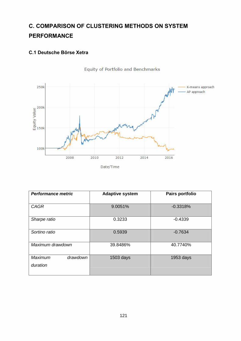
121
C. COMPARISON OF CLUSTERING METHODS ON SYSTEM
PERFORMANCE
C.1 Deutsche Börse Xetra
Performance metric Adaptive system Pairs portfolio
CAGR 9.0051% -0.3318%
Sharpe ratio 0.3233 -0.4339
Sortino ratio 0.5939 -0.7634
Maximum drawdown 39.8486% 40.7740%
Maximum drawdown
duration
1503 days 1953 days

122
C.2 TSE ETFs
Performance metric Adaptive system Pairs portfolio
CAGR 3.7382% 1.9051%
Sharpe ratio -0.0828 -0.3011
Sortino ratio -0.1496 -0.5539
Maximum drawdown 18.1816% 23.6332%
Maximum drawdown
duration
1336 days 1790 days
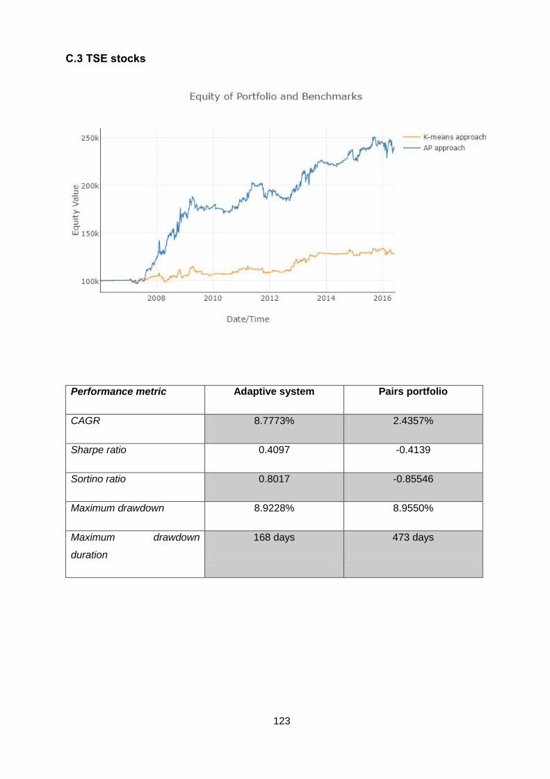
123
C.3 TSE stocks
Performance metric Adaptive system Pairs portfolio
CAGR 8.7773% 2.4357%
Sharpe ratio 0.4097 -0.4139
Sortino ratio 0.8017 -0.85546
Maximum drawdown 8.9228% 8.9550%
Maximum drawdown
duration
168 days 473 days

124
C.4 JSE stocks
Performance metric Adaptive system Pairs portfolio
CAGR 4.9076% 2.7149%
Sharpe ratio 0.0198 -0.3548
Sortino ratio 0.0381 -0.6869
Maximum drawdown 29.8682% 12.0018%
Maximum drawdown
duration
1069 days 1728 days

125
C.5 US ETFs
Performance metric Adaptive system Pairs portfolio
CAGR 7.8518% 1.9743%
Sharpe ratio 0.3945 -1.0852
Sortino ratio 0.8136 -2.1893
Maximum drawdown 7.6237% 2.6126%
Maximum drawdown
duration
106 days 204 days

126
C.6 US stocks
Performance metric Adaptive system Pairs portfolio
CAGR 7.1178% 2.9982%
Sharpe ratio 0.2175 -0.1367
Sortino ratio 0.4072 -0.2517
Maximum drawdown 21.4063% 21.5728%
Maximum drawdown
duration
622 days 835 days
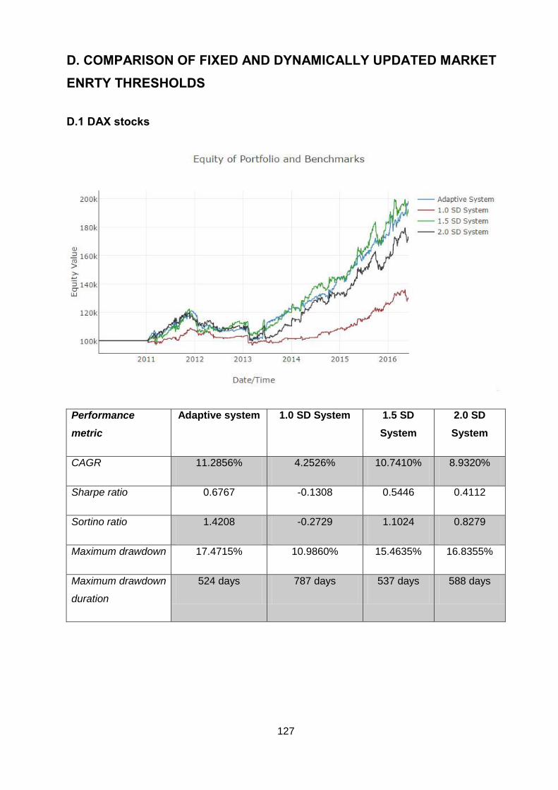
127
D. COMPARISON OF FIXED AND DYNAMICALLY UPDATED MARKET
ENRTY THRESHOLDS
D.1 DAX stocks
Performance
metric
Adaptive system 1.0 SD System 1.5 SD
System
2.0 SD
System
CAGR 11.2856% 4.2526% 10.7410% 8.9320%
Sharpe ratio 0.6767 -0.1308 0.5446 0.4112
Sortino ratio 1.4208 -0.2729 1.1024 0.8279
Maximum drawdown 17.4715% 10.9860% 15.4635% 16.8355%
Maximum drawdown
duration
524 days 787 days 537 days 588 days

128
D.2 JSE stocks
Performance
metric
Adaptive system 1.0 SD System 1.5 SD
System
2.0 SD
System
CAGR 5.9812% 4.2830% 3.6340% 6.4629%
Sharpe ratio 0.1184 -0.0624 -0.1803 0.1748
Sortino ratio 0.2265 -0.1104 -0.3921 0.3320
Maximum drawdown 13.1881% 9.8410% 7.0589% 8.1061%
Maximum drawdown
duration
320 days 121 days 422 days 65 days

129
D.3 US stocks
Performance
metric
Adaptive system 1.0 SD System 1.5 SD
System
2.0 SD
System
CAGR 6.7422% 8.7813% 5.9075% 4.1397%
Sharpe ratio 0.2798 0.4927 0.1430 -0.1678
Sortino ratio 0.5867 1.0514 0.3002 -0.3364
Maximum drawdown 6.7218% 6.4188% 7.0440% 5.2134%
Maximum drawdown
duration
437 days 170 days 91 days 456 days

130
E. SENSITIVITY ANALYSIS OF TRANSACTION COSTS ON THE
DEUTSCHE BÖRSE XETRA
E.1 Transaction cost of 0.35% of trade value
Performance
metric
Adaptive
system
CAGR 14.9521%
Sharpe ratio 0.7067
Sortino ratio 1.3235
Maximum
drawdown
38.4912%
Maximum
drawdown
duration
806 days
E.2 Transaction cost of 0.40% of trade value
Performance
metric
Adaptive
system
CAGR 9.0051%
Sharpe ratio 0.3233
Sortino ratio 0.5939
Maximum
drawdown
39.8486%
Maximum
drawdown
duration
1503 days

131
E.3 Transaction cost of 0.45% of trade value
Performance
metric
Adaptive
system
CAGR 3.3655%
Sharpe ratio -0.0610
Sortino ratio -0.1103
Maximum
drawdown
41.5248%
Maximum
drawdown
duration
1960 days
E.4 Transaction cost of 0.50% of trade value
Performance
metric
Adaptive
system
CAGR -1.9975%
Sharpe ratio -0.4467
Sortino ratio -0.7934
Maximum
drawdown
50.7367%
Maximum
drawdown
duration
1960 days

132
F. ANALYSIS OF DIFFERENT GARCH-UPDATED MODELS ON THE
ADAPTIVE SYSTEM PERFORMANCE
F.1 DAX stocks
Performance
metric
Adaptive
system
(1.0)
Adaptive
system
(1.5)
Adaptive
system
(2.0)
1.0 SD
System
1.5 SD
System
2.0 SD
System
CAGR 6.0671% 11.2856% 9.8879% 4.2526% 10.7410% 8.9320%
Sharpe ratio 0.1661 0.6767 0.6075 -0.1308 0.5446 0.4112
Sortino ratio 0.3572 1.4208 1.2554 -0.2729 1.1024 0.8279
Maximum
drawdown
5.814% 17.4715 11.1662 10.9860% 15.4635% 16.8355%
Maximum
drawdown
duration
357 days 524 days 487 days 787 days 537 days 588 days

133
F.2 JSE Stocks
Performance
metric
Adaptive
system
(1.0)
Adaptive
system
(1.5)
Adaptive
system
(2.0)
1.0 SD
System
1.5 SD
System
2.0 SD
System
CAGR 5.0470% 5.9812% 6.0501% 4.2830% 3.6340% 6.4629%
Sharpe ratio 0.0203 0.1184 0.1241 -0.0624 -0.1803 0.1748
Sortino ratio 0.0388 0.2265 0.2375 -0.1104 -0.3921 0.3320
Maximum
drawdown
14.3967% 13.1881% 11.9125% 9.8410% 7.0589% 8.1061%
Maximum
drawdown
duration
368 days 320 days 297 days 121 days 422 days 65 days

134
F.3 US Stocks
Performance
metric
Adaptive
system
(1.0)
Adaptive
system
(1.5)
Adaptive
system
(2.0)
1.0 SD
System
1.5 SD
System
2.0 SD
System
CAGR 6.7132% 6.7422% 5.2770% 8.7813% 5.9075% 4.1397%
Sharpe ratio 0.2178 0.2798 0.0556 0.4927 0.1430 -0.1678
Sortino ratio 0.4438 0.5867 0.1126 1.0514 0.3002 -0.3364
Maximum
drawdown
16.4958% 6.7218% 7.9139% 6.4188% 7.0440% 5.2134%
Maximum
drawdown
duration
261 days 437 days 305 days 170 days 91 days 456 days
Recommended