1
Ambiguity and Social Judgment: Fuzzy Set Model and Data Analysis
Kazuhisa Takemura Waseda University,
Japan
1. Introduction
Comparative judgment is essential in human social lives. Comparative judgment is a type of human judgment procedure, in which the evaluator is asked which alternative is preferred (e.g., “Do you prefer Brand A to Brand B?” or “How do you estimate the probability of choosing Brand A over Brand B when you compare the two brands? ”). This type of judgment is distinguished from absolute judgment, in which the evaluator is asked to assess the attractiveness of an object (e.g., “How much do you like this brand on a scale of 0 to 100?”).
The ambiguity of social judgment has been conceptualized by the fuzzy set theory. The
fuzzy set theory provides a formal framework for the presentation of the ambiguity. Fuzzy
sets were defined by Zadeh(1965) who also outlined how they could be used to characterize
complex systems and decision processes ( Zadeh, 1973). Zadeh argues that the capacity of
humans to manipulate fuzzy concepts should be viewed as a major asset, not a liability. The
complexities in the real world often defy precise measurement and fuzzy logic defines
concepts and its techniques provide a mathematical method able to deal with thought
processes which are often too imprecise and ambiguous to deal with by classical
mathematical techniques.
This chapter introduces a model of ambiguous comparative judgment (Takemura,2007) and
provides a method of data analysis for the model, and then shows some examples of the
data analysis of social judgments. Comparative judgments in social situations often involve
ambiguity with regard to confidence, and people may be unable to make judgments without
some confidence intervals. To measure the ambiguity (or vagueness) of human judgment,
the fuzzy rating method has been proposed and developed (Hesketh, Pryor, Gleitzman, &
Hesketh, 1988). In fuzzy rating, respondents select a representative rating point on a scale
and indicate higher or lower rating points, depending on the relative ambiguity of their
judgment. For example, fuzzy rating would be useful for perceived temperature, with the
evaluator indicating a representative value and lower and upper values. This rating scale
allows for asymmetries and overcomes the problem, identified by Smithson (1987), of
researchers arbitrarily deciding the most representative value from a range of scores. By
making certain simplifying assumptions (which is not uncommon in fuzzy set theory), the
rating can be viewed as an L-R fuzzy number, thereby making the use of fuzzy set
www.intechopen.com
Fuzzy Logic – Algorithms, Techniques and Implementations
4
theoretical operations possible (Hesketh et al., 1988; Takemura, 2000). Lastly, numerical
illustrations of psychological experiments are provided to examine the ambiguous
comparative judgment model (Takemura, 2007) using the proposed data analysis.
2. Model of ambiguous comparative judgment
2.1 Overview of ambiguous comparative judgment and the judgment model
Social psychological theory and research have demonstrated that comparative evaluation
has a crucial role in the cognitive processes and structures that underlie people’s judgments,
decisions, and behaviors(e.g.,Mussweiler,2003). People comparison processes are almost
ubiquitous in human social cognition. For example, people tend to compare their
performance of others in situations that are ambiguous (Festinger,1954). It is also obvious
that they are critical in forming personal evaluations, and making purchase decisions
(Kühberger,,.Schulte-Mecklenbeck, & Ranyard, 2011; Takemura,2011).
The ambiguity or vagueness is inherent in people's comparative social judgment.
Traditionally, psychological and philosophical theories implicitly had assumed the
ambiguity of thought processes ( Smithson, 1987, 1989). For example, Wittgenstein (1953)
pointed out that lay categories were better characterized by a “ family resemblance” model
which assumed vague boundaries of concepts rather than a classical set-theoretic model.
Rosch (1975) and Rosch & Mervice(1975) also suggested vagueness of lay categories in her
prototype model and reinterpret-ed the family resemblance model. Moreover, the social
judgment theory (Sherif & Hovland,1961) and the information integration theory
(Anderson,1988) for describing judgment and decision making assumed that people
evaluate the objects using natural languages which were inherently ambiguous. However,
psychological theories did not explicitly treat the ambiguity in social judgment with the
exception of using random error of judgment.
Takemura (2007) proposed fuzzy set models that explain ambiguous comparative judgment
in social situations. Because ambiguous comparative judgment may not always hold
transitivity and comparability properties, the models assume parameters based on biased
responses that may not hold transitivity and comparability properties. The models consist of
two types of fuzzy set components for ambiguous comparative judgment. The first is a
fuzzy theoretical extension of the additive difference model for preference, which is used to
explain ambiguous preference strength and does not always assume judgment scale
boundaries, such as a willing to pay (WTP) measure. The second type of model is a fuzzy
logistic model of the additive difference preference, which is used to explain ambiguous
preference in which preference strength is bounded, such as a probability measure (e.g., a
certain interval within a bounded interval from 0 to 100%).
Because judgment of a bounded scale, such as a probability judgment, causes a
methodological problem when fuzzy linear regression is used, a fuzzy logistic function to
prevent this problem was proposed. In both models, multi-attribute weighting parameters
and all attribute values are assumed to be asymmetric fuzzy L-R numbers. For each model,
A method of parameter estimation using fuzzy regression analysis was proposed. That is, a
fuzzy linear regression model using the least squares method (Takemura, 1999, 2005) was
www.intechopen.com
Ambiguity and Social Judgment: Fuzzy Set Model and Data Analysis
5
applied for the analysis of the former model, and a fuzzy logistic regression model
(Takemura, 2004) was proposed for the analysis of the latter model.
2.2 Assumptions of the model
2.2.1 Definition 1: Set of multidimensional alternatives
Let X = X1× X2 × …. × Xn be a set of multidimensional alternatives with elements of the form
X1 = (X11, X12,…,X1n), X2 = (X21, X22,…,X2n),…, Xm = (Xm1, Xm2,…,Xmn), where Xij (i = 1.m;
j = 1.,n) is the value of alternative Xi on dimension j. Note that the components of Xi may be
ambiguous linguistic variables rather than crisp numbers.
2.2.2 Definition 2: Classic preference relation
Let be a binary relation on X, that is, is a subset of X × X.
The relational structure < X, > is a weak order if, and only if, for all Xa, Xb, Xc, the
following two axioms are satisfied.
1. Connectedness (Comparability): Xa, Xb or Xb Xa,
2. Transitivity: If Xa Xb and Xb Xc, then Xa Xc.
However, the weak order relation is not always assumed in this paper. That is, transitivity
or connectedness may be violated in the preference relations.
2.2.3 Definition 3: Fuzzy preference relation
As a classical preference relation is a subset of X × X , is a classical set often viewed as a
characteristic function c from X × X to {0,1} such that:
c(Xj Xk) = a b
a b
1 iff X X
0 iff not(X X )
.
Note that “iff” is short for “if and only if” and {0,1} is called the valuation set. If the
valuation set is allowed to be the real interval [0,1], is called a fuzzy preference relation.
That is, the membership function µa is defined as:
µa: X × X → [0,1].
2.2.4 Definition 4: Ambiguous preference relation
Ambiguous preference relations are defined as a fuzzy set of X ×X × S, where S is a subset
of one-dimensional real number space. S is interpreted as a domain of preference strength. S
may be bounded, for example, S = [0,1]. The membership function µβ is defined as:
µと:: X × X × S → [0,1].
www.intechopen.com
Fuzzy Logic – Algorithms, Techniques and Implementations
6
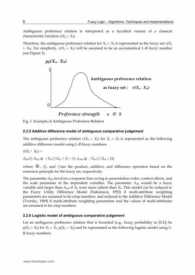
Ambiguous preference relation is interpreted as a fuzzified version of a classical
characteristic function c(Xa Xb).
Therefore, the ambiguous preference relation for Xa Xb is represented as the fuzzy set v(Xa
Xb). For simplicity, v(Xa Xb) will be assumed to be an asymmetrical L-R fuzzy number
(see Figure 1).
μβ(Xa Xb)
1
Ambiguous preference relation
as fuzzy set : v(Xa Xb)
0
Preference strength s ∈ S
Fig. 1. Example of Ambiguous Preference Relation
2.2.5 Additive difference model of ambiguous comparative judgement
The ambiguous preference relation v(Xa Xb) for Xa Xb is represented as the following
additive difference model using L-R fuzzy numbers:
v(Xa Xb)=
Aab0○+ Aab1 ⊗うXa1○-Xb1え○+…○+Aabn ⊗うXan○--Xbnえ(1)
where ⊗ , ○+, and ○-are the product, additive, and difference operation based on the
extension principle for the fuzzy set, respectively.
The parameter Ajk0 involves a response bias owing to presentation order, context effects, and the scale parameter of the dependent variables. The parameter Ajk0 would be a fuzzy variable and larger than Aab0 if Xa were more salient than Xb. This model can be reduced to the Fuzzy Utility Difference Model (Nakamura, 1992) if multi-attribute weighting parameters are assumed to be crisp numbers, and reduced to the Additive Difference Model (Tversky, 1969) if multi-attribute weighting parameters and the values of multi-attributes are assumed to be crisp numbers.
2.2.6 Logistic model of ambiguous comparative judgement
Let an ambiguous preference relation that is bounded (e.g., fuzzy probability in [0,1]) be
p(Xa Xb) for Xa Xb. p(Xa Xb) and be represented as the following logistic model using L-
R fuzzy numbers:
www.intechopen.com
Ambiguity and Social Judgment: Fuzzy Set Model and Data Analysis
7
log ( p(Xa Xb) ○÷う1 ○-p(Xj Xk)え= 1nXb1)ype correction and drawing figures.mments and
Aab0○+ Aab1 ⊗うXa1○-Xb1え ○+…○+Aabn ⊗ (Xan○--Xbnえ (2)
where log, ○÷ , ⊗ ,○+, and ○- are logarithmic, division, product , additive, and difference
operations based on the extension principle for the fuzzy set, respectively.
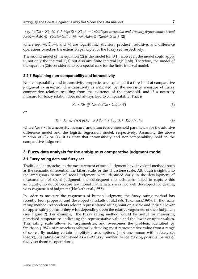
The second model of the equation (2) is the model for [0,1]. However, the model could apply to not only the interval [0,1] but also any finite interval [a,b](a<b). Therefore, the model of the equation (2)is considered to be a special case for the finite interval model.
2.2.7 Explaining non-comparability and intransitivity
Non-comparability and intransitivity properties are explained if a threshold of comparative judgment is assumed, if intransitivity is indicated by the necessity measure of fuzzy comparative relation resulting from the existence of the threshold, and if a necessity measure for fuzzy relation does not always lead to comparability. That is,
Xa Xb iff Nes ( v(Xa Xb)>θ) (3)
or
Xa Xb iff Nes( p(Xa Xb) ○÷う1 ○-p(Xa Xb) )> Pθ) (4)
where Nes (・) is a necessity measure, and θ, and Pθ are threshold parameters for the additive
difference model and the logistic regression model, respectively. Assuming the above relation of (3) or (4), it is clear that intransitivity and non-comparability hold in the comparative judgment.
3. Fuzzy data analysis for the ambiguous comparative judgment model
3.1 Fuzzy rating data and fuzzy set
Traditional approaches to the measurement of social judgment have involved methods such as the semantic differential, the Likert scale, or the Thurstone scale. Although insights into the ambiguous nature of social judgment were identified early in the development of measurement of social judgment, the subsequent methods used failed to capture this ambiguity, no doubt because traditional mathematics was not well developed for dealing with vagueness of judgment (Hesketh et al.,1988).
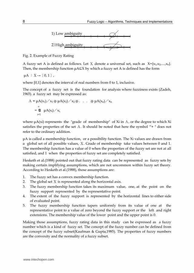
In order to measure the vagueness of human judgment, the fuzzy rating method has recently been proposed and developed (Hesketh et al.,1988; Takemura,1996). In the fuzzy rating method, respondents select a representative rating point on a scale and indicate lower or upper rating points if they wish depending upon the relative vagueness of their judgment (see Figure 2). For example, the fuzzy rating method would be useful for measuring perceived temperature indicating the representative value and the lower or upper values. This rating scale allows for asymmetries, and overcomes the problem, identified by Smithson (1987), of researchers arbitrarily deciding most representative value from a range of scores. By making certain simplifying assumptions ( not uncommon within fuzzy set theory), the rating can be viewed as a L-R fuzzy number, hence making possible the use of fuzzy set theoretic operations).
www.intechopen.com
Fuzzy Logic – Algorithms, Techniques and Implementations
8
1) Low ambiguity
2䐢High ambiguity
Fig. 2. Example of Fuzzy Rating
A fuzzy set A is defined as follows. Let X denote a universal set, such as X={x1,x2,....,xn}.
Then, the membership function μA⊆X by which a fuzzy set A is defined has the form
μA :X→[0, 1],
where [0,1] denotes the interval of real numbers from 0 to 1, inclusive.
The concept of a fuzzy set is the foundation for analysis where fuzziness exists (Zadeh, 1965). a fuzzy set may be expressed as:
A = μA(x1)Ǹx1 ⊕ μA(x2)Ǹx2 ⊕ ḿḿḿ ⊕ μA(xn)Ǹxn
n
= Σ μA(xi)Ǹxi,
i=1
where μA(xi) represents the "grade of membership" of Xi in A, or the degree to which Xi
satisfies the properties of the set A. It should be noted that here the symbol '"+ " does not
refer to the ordinary addition.
μA is called a membership function, or a possibility function. The Xi values are drawn from
a global set of all possible values, X. Grade of membership take values between 0 and 1.
The membership function has a value of 0 when the properties of the fuzzy set are not at all
satisfied, and 1 when the properties of fuzzy set are completely satisfied.
Hesketh et al.(1988) pointed out that fuzzy rating data can be represented as fuzzy sets by
making certain implifying assumptions, which are not uncommon within fuzzy set theory.
According to Hesketh et al.(1988), those assumptions are:
1. The fuzzy set has a convex membership function.
2. The global set X is represented along the horizontal axis.
3. The fuzzy membership function takes its maximum value, one, at the point on the
fuzzy support represented by the representative point.
4. The extent of the fuzzy support is represented by the horizontal lines to either side
of evaluated point.
5. The fuzzy membership function tapers uniformly from its value of one at the
representative point to a value of zero beyond the fuzzy support or the left and right
extensions. The membership value of the lower point and the upper point is 0.
Making those assumptions, fuzzy rating data in this study can be expressed as a fuzzy
number which is a kind of fuzzy set. The concept of the fuzzy number can be defined from
the concept of the fuzzy subset(Kaufman & Gupta,1985). The properties of fuzzy numbers
are the convexity and the normality of a fuzzy subset.
www.intechopen.com
Ambiguity and Social Judgment: Fuzzy Set Model and Data Analysis
9
Firstly, the convexity of the fuzzy subset is defined as follows: A fuzzy subset A ⊆ R is convex if and only if every ordinary
Aα= {x| μA(x) ≧ α}, α∈[0,1],
subset is convex( That is, in the case of a closed interval of R).
Secondly, the normality of the fuzzy subset is defined as follows: A fuzzy subset A ⊆ R is normal if and only if ∀x ∈R, max μA(x) = 1.
x
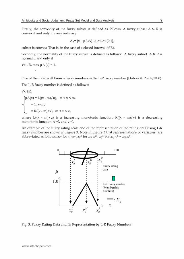
One of the most well known fuzzy numbers is the L-R fuzzy number (Dubois & Prade,1980).
The L-R fuzzy number is defined as follows: ∀x ∈R:
μA(x) = L((x - m)/u), - ∞ < x < m,
= 1, x=m,
= R((x - m)/v), m < x < ∞,
where L((x - m)/u) is a increasing monotonic function, R((x - m)/v) is a decreasing monotonic function, u>0, and v>0.
An example of the fuzzy rating scale and of the representation of the rating data using L-R fuzzy number are shown in Figure 3. Note in Figure 3 that representations of variables are abbreviated as follows: xijL for xi j (0lL, xijR for xi j (0lR , xijM for xi j (1lL = xi j (1lR.
Fig. 3. Fuzzy Rating Data and Its Representation by L-R Fuzzy Numbers
µ
x
0.1
L
ijx
ijX:
0
100
M
ijxR
ijx
Fuzzy rating
data
L-R fuzzy number
(Membership
function)
L
ijxM
ijxR
ijx
www.intechopen.com
Fuzzy Logic – Algorithms, Techniques and Implementations
10
3.2 Analysis of the additive difference type model
The set of fuzzy input-output data for the k-th observation is defined as:
( )abk a1k a2k ank ; b1k b2 k bnk;Y ;X , X , ,X X ,X , ,X (5)
where Yabk indicates the k-th observation’s ambiguous preference for the a-th alternative (a)
over the b-th alternative (b), which represented by fuzzy L-R numbers, and Xajk and Xbjk are
the j-th attribute values of the alternatives (a and b) for observation k.
Let Xabjk be Xajk - Xbjk, where - is a difference operator based on the fuzzy extension
principle, and denote Xk. as the abbreviation of Xabk in the following section. Therefore, a set
of fuzzy input-output data for the i-th observation is re-written as:
( )k 1k 2k nkY ;X ,X , ,X , k=1,2,….,N (6)
where Yk is a fuzzy dependent variable, and Xjk is a fuzzy independent variable represented by L-R fuzzy numbers. For simplicity, assume that Yk and Xjk are positive for any
membership value, α ∈ (0,1).
The fuzzy linear regression model (where both input and output data are fuzzy numbers) is represented as follows:
k 0 1 1k n nkY A A X A X= ⊕ ⊗ ⊕ ⊕ ⊗ (7)
where is a fuzzy estimated variable, Aj(j = 1,…,n) is a fuzzy regression parameter
represented by an L-R fuzzy number, ⊗ is an additive operator, and ⊕ is the product operator based on the extension principle.
It should be noted that although the explicit form of the membership function of kY cannot
be directly obtained, the α-level set of kY can be obtained from Nguyen’s theorem (Nguyen,
1978).
Let ( )Lkz α be a lower value of kY , and ( )
Rkz α be an upper value of kY .
Then,
( ) ( ) ( ]L Rk k kZ z ,z , 0,1α α
= α ∈ (8)
Where
( ) ( ) ( ) ( ) ( )( ){ }n
L L L L Rk j jk j jk
j 0
z min a x ,a xα α α α α=
= (9)
( ) ( ) ( ) ( ) ( )( ){ }n
R R L R Rk j jk j jk
j 0
z max a x ,a xα α α α α=
= (10)
www.intechopen.com
Ambiguity and Social Judgment: Fuzzy Set Model and Data Analysis
11
( )Lkx α0 = ( )
Rkx α0 =1 (11)
In the above Equation (9), ( ) ( )L Lj jka xα α is a product between the lower value of the α-level
fuzzy coefficient for the j-th attribute and the α-level set of fuzzy input data Xjk, ( ) ( )L Rj jka xα α ,
( ) ( )R Lj jka xα α , or ( ) ( )
R Rj jka xα α is defined in the same manner, respectively. ( )
L0kx α and ( )
R0kx α are
assumed to be 1 (a crisp number) for the purpose of estimation for the fuzzy bias parameter A0.
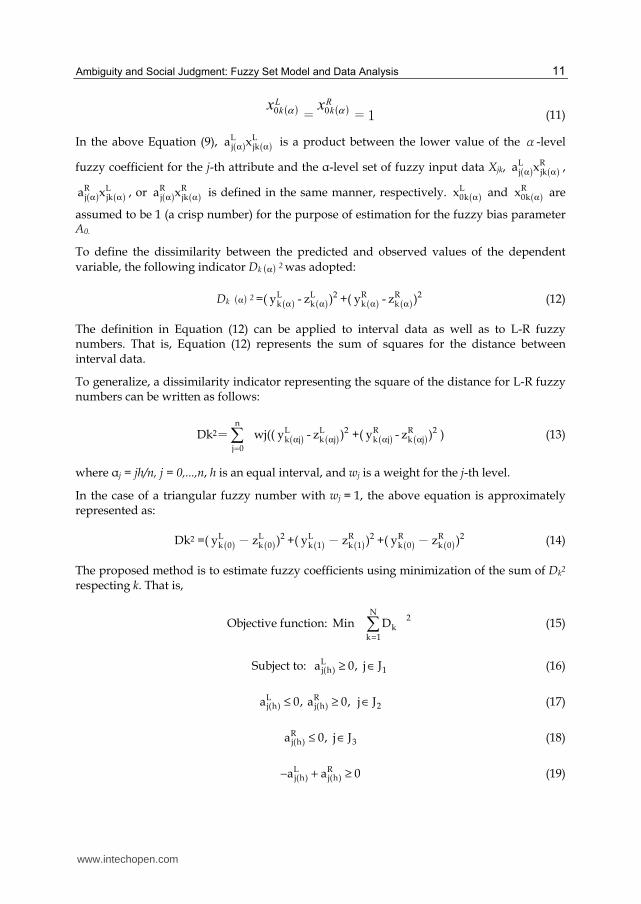
To define the dissimilarity between the predicted and observed values of the dependent
variable, the following indicator Dk ( )α 2 was adopted:
Dk ( )α 2 =( ( )Lky α - ( )
L 2kz )α +( ( )
Rky α - ( )
R 2kz )α (12)
The definition in Equation (12) can be applied to interval data as well as to L-R fuzzy numbers. That is, Equation (12) represents the sum of squares for the distance between interval data.
To generalize, a dissimilarity indicator representing the square of the distance for L-R fuzzy numbers can be written as follows:
Dk2=n
j 0= wj(( ( )
Lk jy α - ( )
L 2k jz )α +( ( )
Rk jy α - ( )
R 2k jz )α ) (13)
where αj = jh/n, j = 0,...,n, h is an equal interval, and wj is a weight for the j-th level.
In the case of a triangular fuzzy number with wj = 1, the above equation is approximately represented as:
Dk2 =( ( )Lk 0y - ( )
L 2k 0z ) +( ( )
Lk 1y - ( )
R 2k 1z ) +( ( )
Rk 0y - ( )
R 2k 0z ) (14)
The proposed method is to estimate fuzzy coefficients using minimization of the sum of Dk2 respecting k. That is,
Objective function: N
2k
k 1
Min D= (15)
Subject to: Lj(h) 1a 0, j J≥ ∈ (16)
L Rj(h) j(h) 2a 0, a 0, j J≤ ≥ ∈ (17)
Rj(h) 3a 0, j J≤ ∈ (18)
L Rj(h) j(h)a a 0− + ≥ (19)
www.intechopen.com
Fuzzy Logic – Algorithms, Techniques and Implementations
12
Where { } 1 2 3j 0,....,n J J J ,∈ = ∪ ∪ 1 2 2 3 3 1J J , J J , J J ,∩ = ϕ ∩ = ϕ ∩ = ϕ
( ) ( ) ( ) ( ) ( )1 2 3
L L L L Rk j jk j jk
j J j J J
z a x a x∈ ∈
α α α α α= + (20)
( ) ( ) ( ) ( ) ( )1, 12 3
R R R R Lk j jk j jk
j J J j J
z a x a x∈ ∈
α α α α α= + (21)
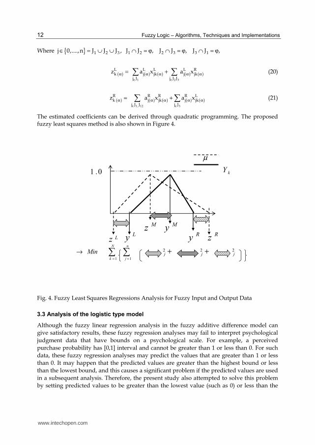
The estimated coefficients can be derived through quadratic programming. The proposed fuzzy least squares method is also shown in Figure 4.
µ
0.1
RzLzLy Ry
kY
Mz My
+2j
==
→n
j
N
k
Min11
+2j
2j
Fig. 4. Fuzzy Least Squares Regressions Analysis for Fuzzy Input and Output Data
3.3 Analysis of the logistic type model
Although the fuzzy linear regression analysis in the fuzzy additive difference model can
give satisfactory results, these fuzzy regression analyses may fail to interpret psychological
judgment data that have bounds on a psychological scale. For example, a perceived
purchase probability has [0,1] interval and cannot be greater than 1 or less than 0. For such
data, these fuzzy regression analyses may predict the values that are greater than 1 or less
than 0. It may happen that the predicted values are greater than the highest bound or less
than the lowest bound, and this causes a significant problem if the predicted values are used
in a subsequent analysis. Therefore, the present study also attempted to solve this problem
by setting predicted values to be greater than the lowest value (such as 0) or less than the
www.intechopen.com
Ambiguity and Social Judgment: Fuzzy Set Model and Data Analysis
13
highest value (such as 1). The present study develops the concept of logistic regression for
the crisp numbers, and then proposes the fuzzy version of logistic regression analysis for
fuzzy input and output data.
The set of fuzzy input-output data for the k-th observation is defined as:
( )abk a1k a2k ank b1k b2k bnkP ;X ,X , ,X ;X ,X , ,X (22)
where Pabk indicates the k-th observation’s ambiguous preference for the a-th alternative (a) over the b-th alternative (b), which is represented by fuzzy L-R numbers, and Xajk and Xbjk
are the j-th attribute values of the alternatives (a and b) for observation k.
Let Xabjk be Xajk ○- Xbjk, where ○- is a difference operator based on the fuzzy extension
principle, and denote Xk. as the abbreviation of Xabk in the following section. Therefore, a set of fuzzy input-output data for the i-th observation is re-written as:
( )k 1k 2k nkP ;X ,X , ,X , k=1,2,….,N (23)
where Pk is a fuzzy dependent variable, and Xjk is a fuzzy independent variable represented by L-R fuzzy numbers. For simplicity, I assume that Pk and Xjk are positive for any
membership value, α ∈ (0,1).
The fuzzy logic regression model (where both input and output data are fuzzy numbers) is represented as follows:
log(Pk ○÷ (1 ○-Pk)) 0 i0 1 i1 m imA X A X A X= ⊗ ⊕ ⊗ ⊕ ⊕ ⊗ (24)
where log(Pk○÷ (1○-Pk)) is the estimated fuzzy log odds, ○÷ is the division operator, ○- is the
difference operator, ⊗ is the product operator, and ⊕ is the additive operator based on the
extension principle for the fuzzy set, respectively.
It should be noted that although the explicit form of the membership function of
log(Pk○÷ (1○-Pk)) cannot be directly obtained, the α -level set of log(Pk○÷ (1○-Pk)) can be
obtained using Nguyen’s theorem (Nguyen, 1978).
Let ( )LkP α be the lower bound of the dependent fuzzy variable and ( )
RkP α be the upper
bound. Then, the α level set of the fuzzy dependent variable Pk can be represented as
( ) ( ) ( ]αL R
k k kP P ,P , 0,1α α = α ∈ .
Therefore, the α level set of the left term in Equation (24) is as follows:
[log(Pk○÷ (1○-Pk))]て=
( ) ( ) ( ) ( )L L R Rk k k k[min(log(P /(1 P )),log(P /(1 P )))α α α α− −
( ) ( ) ( ) ( )L L R Rk k k kmax(log(P /(1 P )),log(P /(1 P )))]α α α α− − (25)
www.intechopen.com

Fuzzy Logic – Algorithms, Techniques and Implementations
14
Let ( )Lkz α be a lower value of [log(Pk○÷ (1○-Pk))]α, and ( )
Rkz α be an upper value of [log(Pk○÷
(1○-Pk))]α
where
( ) ( ) ( ) ( ) ( )( ){ }
nL L L L Rk j jk j jk
j 0
z min a x ,a xα α α α α=
= (26)
( ) ( ) ( ) ( ) ( )( ){ }
nR R L R Rk j jk j jk
j 0
z max a x ,a xα α α α α=
= (27)
( )Lkx α0 = ( )
Rkx α0 =1 (28)
In the above Equation (26), is a product between the lower value of the �-level fuzzy coefficient for the j-th attribute and the α-level set of fuzzy input data Xjk, , or is defined in the same manner, respectively. and are assumed to be 1 (a crisp number) for the purpose of estimation for the fuzzy bias parameter A0. The parameter estimation method is basically the same as the fuzzy logistic regression method and a more concrete procedure is described in Takemura (2004).
4. Numerical example of the data analysis method
To demonstrate the appropriateness of the proposed data analysis methods, the detail numerical examples are shown for the individual level analysis (Takemura,2007) and group level analysis (Takemura, Matsumoto, Matsuyama, & Kobayashi, 2011) of ambiguous comparative judgments.
4.1. Individual level analysis of ambiguous comparative model
4.1.1 Example of additive difference model
4.1.1.1 Participant and procedure
The participant was a 43-year-old faculty member of Waseda University. The participant rated differences in WTP for two different computers (DELL brand) with three types of attribute information (hard disk: 100 or 60 GB; memory: 2.80 or 2.40 GHz; new or used product). The participant compared a certain alternative with seven different alternatives. The participant provided representative values and lower and upper WTP values using a fuzzy rating method. (see Figure 5)
The participant was asked the amount of money he would be willing to pay to upgrade the inferior from inferior alternative to superior alternative using fuzzy rating method. That is, the participant answered the lower value, the representative value, and upper value for the amount of money he would be willing to pay.
Lower Value Representative Value Upper Value
( ) Yen ( ) Yen ( ) Yen
Fig. 5. Example of a Fuzzy Rating in WTP Task.
www.intechopen.com
Ambiguity and Social Judgment: Fuzzy Set Model and Data Analysis
15
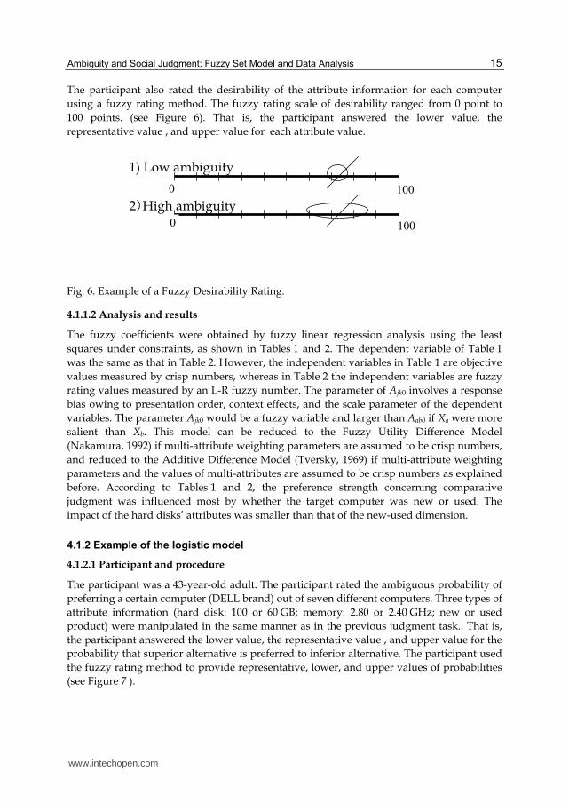
The participant also rated the desirability of the attribute information for each computer
using a fuzzy rating method. The fuzzy rating scale of desirability ranged from 0 point to
100 points. (see Figure 6). That is, the participant answered the lower value, the
representative value , and upper value for each attribute value.
Fig. 6. Example of a Fuzzy Desirability Rating.
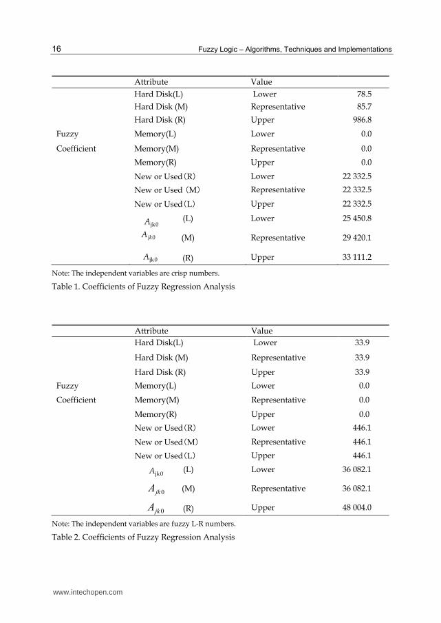
4.1.1.2 Analysis and results
The fuzzy coefficients were obtained by fuzzy linear regression analysis using the least
squares under constraints, as shown in Tables 1 and 2. The dependent variable of Table 1
was the same as that in Table 2. However, the independent variables in Table 1 are objective
values measured by crisp numbers, whereas in Table 2 the independent variables are fuzzy
rating values measured by an L-R fuzzy number. The parameter of Ajk0 involves a response
bias owing to presentation order, context effects, and the scale parameter of the dependent
variables. The parameter Ajk0 would be a fuzzy variable and larger than Aab0 if Xa were more
salient than Xb. This model can be reduced to the Fuzzy Utility Difference Model
(Nakamura, 1992) if multi-attribute weighting parameters are assumed to be crisp numbers,
and reduced to the Additive Difference Model (Tversky, 1969) if multi-attribute weighting
parameters and the values of multi-attributes are assumed to be crisp numbers as explained
before. According to Tables 1 and 2, the preference strength concerning comparative
judgment was influenced most by whether the target computer was new or used. The
impact of the hard disks’ attributes was smaller than that of the new-used dimension.
4.1.2 Example of the logistic model
4.1.2.1 Participant and procedure
The participant was a 43-year-old adult. The participant rated the ambiguous probability of
preferring a certain computer (DELL brand) out of seven different computers. Three types of
attribute information (hard disk: 100 or 60 GB; memory: 2.80 or 2.40 GHz; new or used
product) were manipulated in the same manner as in the previous judgment task.. That is,
the participant answered the lower value, the representative value , and upper value for the
probability that superior alternative is preferred to inferior alternative. The participant used
the fuzzy rating method to provide representative, lower, and upper values of probabilities
(see Figure 7 ).
1) Low ambiguity
2䐢High ambiguity
0
0 100
100
www.intechopen.com
Fuzzy Logic – Algorithms, Techniques and Implementations
16
Attribute Value
Hard Disk(L) Lower 78.5
Hard Disk (M) Representative 85.7
Hard Disk (R) Upper 986.8
Fuzzy Memory(L) Lower 0.0
Coefficient Memory(M) Representative 0.0
Memory(R) Upper 0.0
New or Used膅R䐢 Lower 22 332.5
New or Used 膅M䐢 Representative 22 332.5
New or Used膅L䐢 Upper 22 332.5
(L) Lower 25 450.8
(M) Representative 29 420.1
(R) Upper 33 111.2
Note: The independent variables are crisp numbers.
Table 1. Coefficients of Fuzzy Regression Analysis
Attribute Value
Hard Disk(L) Lower 33.9
Hard Disk (M) Representative 33.9
Hard Disk (R) Upper 33.9
Fuzzy Memory(L) Lower 0.0
Coefficient Memory(M) Representative 0.0
Memory(R) Upper 0.0
New or Used膅R䐢 Lower 446.1
New or Used膅M䐢 Representative 446.1
New or Used膅L䐢 Upper 446.1
(L) Lower 36 082.1
(M) Representative 36 082.1
(R) Upper 48 004.0
Note: The independent variables are fuzzy L-R numbers.
Table 2. Coefficients of Fuzzy Regression Analysis
0jkA
0jkA
0jkA
jk0A
jk0A
jk0A
www.intechopen.com
Ambiguity and Social Judgment: Fuzzy Set Model and Data Analysis
17
1) Low ambiguity
2䐢High ambiguity
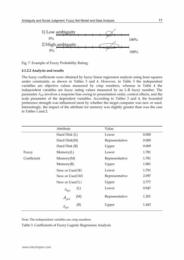
Fig. 7. Example of Fuzzy Probability Rating.
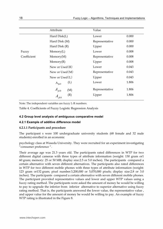
4.1.2.2 Analysis and results
The fuzzy coefficients were obtained by fuzzy linear regression analysis using least squares under constraints, as shown in Tables 3 and 4. However, in Table 3 the independent variables are objective values measured by crisp numbers, whereas in Table 4 the independent variables are fuzzy rating values measured by an L-R fuzzy number. The parameter Ajk0 involves a response bias owing to presentation order, context effects, and the scale parameter of the dependent variables. According to Tables 3 and 4, the bounded preference strength was influenced most by whether the target computer was new or used. Interestingly, the impact of the attribute for memory was slightly greater than was the case in Tables 1 and 2.
Attribute Value
Hard Disk (L) Lower 0.000
Hard Disk(M) Representative 0.000
Hard Disk (R) Upper 0.009
Fuzzy Memory(L) Lower 1.781
Coefficient Memory(M) Representative 1.781
Memory(R) Upper 1.881
New or Used膅R䐢 Lower 1.791
New or Used膅M䐢 Representative 2.097
New or Used膅L䐢 Upper 2.777
(L) Lower 0.847
(M) Representative 1.201
(R) Upper 1.443
Note: The independent variables are crisp numbers.
Table 3. Coefficients of Fuzzy Logistic Regression Analysis
0jkA
0% 100%
100% 0%
jk0A
jk0A
www.intechopen.com
Fuzzy Logic – Algorithms, Techniques and Implementations
18
Attribute Value
Hard Disk(L) Lower 0.000
Hard Disk (M) Representative 0.000
Hard Disk (R) Upper 0.000
Fuzzy Memory(L) Lower 0.008
Coefficient Memory(M) Representative 0.008
Memory(R) Upper 0.008
New or Used膅R䐢 Lower 0.043
New or Used膅M䐢 Representative 0.043
New or Used膅L䐢 Upper 0.043
(L) Lower 1.806
(M) Representative 1.806
(R) Upper 1.806
Note: The independent variables are fuzzy L-R numbers.
Table 4. Coefficients of Fuzzy Logistic Regression Analysis
4.2 Group level analysis of ambiguous comparative model
4.2.1 Example of additive difference model
4.2.1.1 Participants and procedure
The participant s were 100 undergraduate university students (68 female and 32 male students) enrolled in an economic
psychology class at Waseda University. They were recruited for an experiment investigating “consumer preference “.
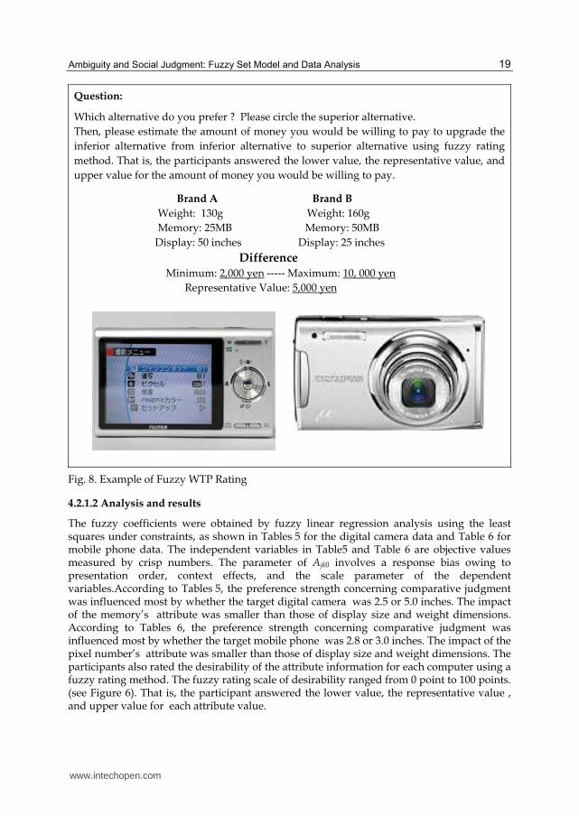
Their average age was 21.3 years old. The participants rated differences in WTP for two different digital cameras with three types of attribute information (weight: 130 gram or1 60 gram; memory: 25 or 50 MB; display size:2.5 or 5.0 inches). The participants compared a certain alternative with seven different alternatives. The participants also rated differences in WTP for two different mobile phones with three types of attribute information (weight: 123 gram or132 gram; pixel number:3,200,000 or 5,070,000 pixels; display size:2.8 or 3.0 inches). The participants compared a certain alternative with seven different mobile phones. The participant provided representative values and lower and upper WTP values using a fuzzy rating method. The participants were asked the amount of money he would be willing to pay to upgrade the inferior from inferior alternative to superior alternative using fuzzy rating method. That is, the participants answered the lower value, the representative value , and upper value for the amount of money he would be willing to pay. An example of fuzzy WTP rating is illustrated in the Figure 8.
0jkA
0jkA
jk0A
www.intechopen.com
Ambiguity and Social Judgment: Fuzzy Set Model and Data Analysis
19
Question:
Which alternative do you prefer ? Please circle the superior alternative.
Then, please estimate the amount of money you would be willing to pay to upgrade the
inferior alternative from inferior alternative to superior alternative using fuzzy rating
method. That is, the participants answered the lower value, the representative value, and
upper value for the amount of money you would be willing to pay.
Brand A Brand B
Weight: 130g Weight: 160g
Memory: 25MB Memory: 50MB
Display: 50 inches Display: 25 inches
Difference
Minimum: 2,000 yen ----- Maximum: 10, 000 yen
Representative Value: 5,000 yen
Fig. 8. Example of Fuzzy WTP Rating
4.2.1.2 Analysis and results
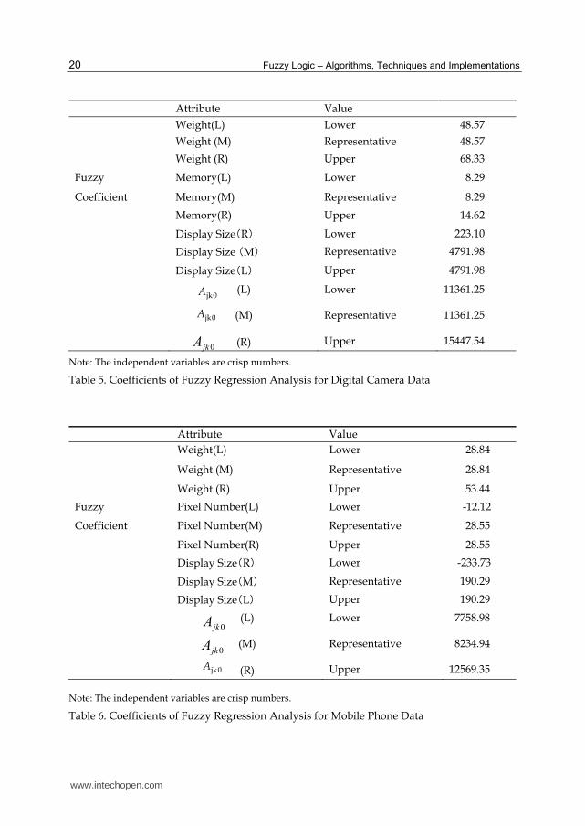
The fuzzy coefficients were obtained by fuzzy linear regression analysis using the least squares under constraints, as shown in Tables 5 for the digital camera data and Table 6 for mobile phone data. The independent variables in Table5 and Table 6 are objective values measured by crisp numbers. The parameter of Ajk0 involves a response bias owing to presentation order, context effects, and the scale parameter of the dependent variables.According to Tables 5, the preference strength concerning comparative judgment was influenced most by whether the target digital camera was 2.5 or 5.0 inches. The impact of the memory’s attribute was smaller than those of display size and weight dimensions. According to Tables 6, the preference strength concerning comparative judgment was influenced most by whether the target mobile phone was 2.8 or 3.0 inches. The impact of the pixel number’s attribute was smaller than those of display size and weight dimensions. The participants also rated the desirability of the attribute information for each computer using a fuzzy rating method. The fuzzy rating scale of desirability ranged from 0 point to 100 points. (see Figure 6). That is, the participant answered the lower value, the representative value , and upper value for each attribute value.
www.intechopen.com
Fuzzy Logic – Algorithms, Techniques and Implementations
20
Attribute Value
Weight(L) Lower 48.57
Weight (M) Representative 48.57
Weight (R) Upper 68.33
Fuzzy Memory(L) Lower 8.29
Coefficient Memory(M) Representative 8.29
Memory(R) Upper 14.62
Display Size膅R䐢 Lower 223.10
Display Size 膅M䐢 Representative 4791.98
Display Size膅L䐢 Upper 4791.98
(L) Lower 11361.25
(M) Representative 11361.25
(R) Upper 15447.54
Note: The independent variables are crisp numbers.
Table 5. Coefficients of Fuzzy Regression Analysis for Digital Camera Data
Attribute Value
Weight(L) Lower 28.84
Weight (M) Representative 28.84
Weight (R) Upper 53.44
Fuzzy Pixel Number(L) Lower -12.12
Coefficient Pixel Number(M) Representative 28.55
Pixel Number(R) Upper 28.55
Display Size膅R䐢 Lower -233.73
Display Size膅M䐢 Representative 190.29
Display Size膅L䐢 Upper 190.29
(L) Lower 7758.98
(M) Representative 8234.94
(R) Upper 12569.35
Note: The independent variables are crisp numbers.
Table 6. Coefficients of Fuzzy Regression Analysis for Mobile Phone Data
0jkA
0jkA
0jkA
jk0A
jk0A
jk0A
www.intechopen.com
Ambiguity and Social Judgment: Fuzzy Set Model and Data Analysis
21
4.2.2 Example of the logistic model
4.2.2.1 Participants and procedure
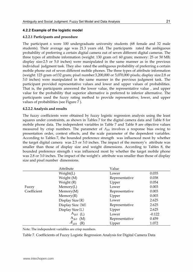
The participant s were 100 undergraduate university students (68 female and 32 male students). Their average age was 21.3 years old. The participants rated the ambiguous probability of preferring a certain digital camera out of seven different digital cameras. The three types of attribute information (weight: 130 gram or1 60 gram; memory: 25 or 50 MB; display size:2.5 or 5.0 inches) were manipulated in the same manner as in the previous individual judgment task. They also rated the ambiguous probability of preferring a certain mobile phone out of seven different mobile phones. The three types of attribute information (weight: 123 gram or132 gram; pixel number:3,200,000 or 5,070,000 pixels; display size:2.8 or 3.0 inches) were manipulated in the same manner in the previous judgment task. The participant provided representative values and lower and upper values of probabilities. That is, the participants answered the lower value, the representative value , and upper value for the probability that superior alternative is preferred to inferior alternative. The participants used the fuzzy rating method to provide representative, lower, and upper values of probabilities (see Figure 7 ).
4.2.2.2 Analysis and results
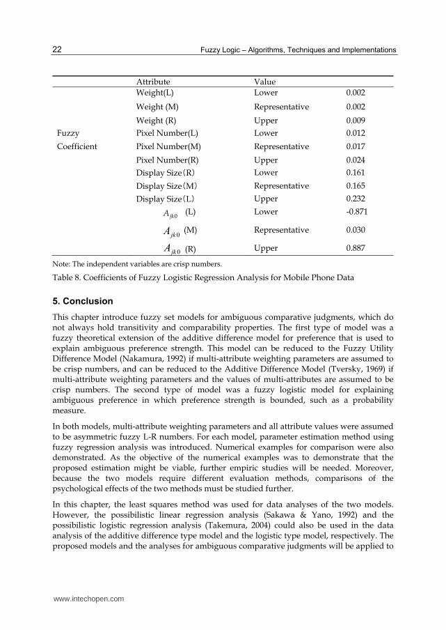
The fuzzy coefficients were obtained by fuzzy logistic regression analysis using the least squares under constraints, as shown in Tables 7 for the digital camera data and Table 8 for mobile phone data. The independent variables in Table 7 and Table 8 are objective values measured by crisp numbers. The parameter of Ajk0 involves a response bias owing to presentation order, context effects, and the scale parameter of the dependent variables. According to Tables 7, the bounded preference strength was influenced most by whether the target digital camera was 2.5 or 5.0 inches. The impact of the memory’s attribute was smaller than those of display size and weight dimensions. According to Tables 8, the bounded preference strength t was influenced most by whether the target mobile phone was 2.8 or 3.0 inches. The impact of the weight’s attribute was smaller than those of display size and pixel number dimensions.
Attribute Value
Weight(L) Lower 0.035 Weight (M) Representative 0.038 Weight (R) Upper 0.054 Fuzzy Memory(L) Lower 0.003 Coefficient Memory(M) Representative 0.003 Memory(R) Upper 0.003 Display Size膅R䐢 Lower 2.625
Display Size 膅M䐢 Representative 2.625
Display Size膅L䐢 Upper 2.625
(L) Lower -0.122 (M) Representative 0.459 (R) Upper 1.072
Note: The independent variables are crisp numbers.
Table 7. Coefficients of Fuzzy Logistic Regression Analysis for Digital Camera Data
0jkA
jk0A
jk0A
www.intechopen.com
Fuzzy Logic – Algorithms, Techniques and Implementations
22
Attribute Value
Weight(L) Lower 0.002
Weight (M) Representative 0.002
Weight (R) Upper 0.009
Fuzzy Pixel Number(L) Lower 0.012
Coefficient Pixel Number(M) Representative 0.017
Pixel Number(R) Upper 0.024
Display Size膅R䐢 Lower 0.161
Display Size膅M䐢 Representative 0.165
Display Size膅L䐢 Upper 0.232
(L) Lower -0.871
(M) Representative 0.030
(R) Upper 0.887
Note: The independent variables are crisp numbers.
Table 8. Coefficients of Fuzzy Logistic Regression Analysis for Mobile Phone Data
5. Conclusion
This chapter introduce fuzzy set models for ambiguous comparative judgments, which do not always hold transitivity and comparability properties. The first type of model was a fuzzy theoretical extension of the additive difference model for preference that is used to explain ambiguous preference strength. This model can be reduced to the Fuzzy Utility Difference Model (Nakamura, 1992) if multi-attribute weighting parameters are assumed to be crisp numbers, and can be reduced to the Additive Difference Model (Tversky, 1969) if multi-attribute weighting parameters and the values of multi-attributes are assumed to be crisp numbers. The second type of model was a fuzzy logistic model for explaining ambiguous preference in which preference strength is bounded, such as a probability measure.
In both models, multi-attribute weighting parameters and all attribute values were assumed to be asymmetric fuzzy L-R numbers. For each model, parameter estimation method using fuzzy regression analysis was introduced. Numerical examples for comparison were also demonstrated. As the objective of the numerical examples was to demonstrate that the proposed estimation might be viable, further empiric studies will be needed. Moreover, because the two models require different evaluation methods, comparisons of the psychological effects of the two methods must be studied further.
In this chapter, the least squares method was used for data analyses of the two models. However, the possibilistic linear regression analysis (Sakawa & Yano, 1992) and the possibilistic logistic regression analysis (Takemura, 2004) could also be used in the data analysis of the additive difference type model and the logistic type model, respectively. The proposed models and the analyses for ambiguous comparative judgments will be applied to
0jkA
0jkA
0jkA
www.intechopen.com
Ambiguity and Social Judgment: Fuzzy Set Model and Data Analysis
23
marketing research, risk perception research, and human judgment and decision-making research. Empirical research using possibilistic analysis and least squares analysis will be needed to examine the validity of these models.
Results of these applications to psychological study indicated that the parameter estimated in the proposed analysis was meaningful for social judgment study. This study has a methodological restriction on statistical inferences for fuzzy parameters. Therefore, we plan further work on the fuzzy theoretic analysis of social judgment directed toward the statistical study of fuzzy regression analysis and fuzzy logistic regression analysis such as statistical tests of parameters, outlier detection, and step-wise variable selection.
6. Acknowledgment
This work was supported in part by Grants in Aids for Grant-in-Aid for Scientific Research on Priority Area, The Ministry of Education, Culture, Sports, Science and Technology(MEXT). I thank Matsumoto,T., Matsuyama,S.,and Kobayashi,M.. for their assistance, and the editor and the reviewers for their valuable comments.
7. References
Anderson,N.H.(1988). A functional approach to person cognition. In T.K.Srull & R.S. Wyer (Eds.), Advances in social cognition. vol.1. Hiisdale, New Jersey: Lawrence Erlbaum Associates, pp.37-51.
Dubois D. & Prade,H. (1980). Fuzzy sets and systems: Theory and applications, New York: Academic Press.
Festinger, L. (1954). A theory of social comparison processes. Human Relations, 7, 114–140. Hesketh, B., Pryor, R., Gleitzman, M., & Hesketh, T. (1988). Practical applications and
psychometric evaluation of a computerised fuzzy graphic rating scale. In T. Zetenyi (Ed.), Fuzzy sets in psychology (pp. 425–454). New York: North Holland.
Kühberger,A.,.Schulte-Mecklenbeck,M. & Ranyard,R. (2011). Introduction: Windows for understanding the mind, In M.Schulte-Mecklenbeck, A.Kühberger, & R. Ranyard(Eds.), A handbook of process tracing methods for decision research,New Yorrk: Psychologgy Press, pp.3-17.
Mussweiler, T. (2003). Comparison processes in social judgment: Mechanisms and consequences. Psychological Review, 110, 472–489.
Nakamura, K. (1992). On the nature of intransitivity in human referential judgments. In V. Novak (Ed.), Fuzzy approach to reasoning and decision making, academia (pp. 147–162). Prague: Kluwer Academic Publishers.
Nguyen, H. T. (1978). A note on the extension principle for fuzzy sets. Journal of Mathematical Analysis and Application, 64, 369–380.
Rosch,E. (1975). Cognitive representation of semantic categories. Journal of Experimental Psychology: General, 104, 192-233.
Rosch,E., & Mervis,C.B. (1975). Family resemblances: Studies in the internal structure of categories. Cognitive Psychology, 7, 573-603.
Sakawa, M., & Yano, H. (1992). Multiobjective fuzzy linear regression analysis for fuzzy input-output data. Fuzzy Sets and Systems, 47, 173–181.
www.intechopen.com
Fuzzy Logic – Algorithms, Techniques and Implementations
24
Sherif,M.,& Hovland,C,I. (1961). Social judgment: Assimilation and contrast effects in communication and attitude change. New Haven: Yale University Press.
Smithson, M. (1987). Fuzzy set analysis for the behavioral and social sciences. New York: Springer-Verlag.
Smithson,M.(1989) Ignorance and uncertainty. New York: Springer-Verlag- Takemura, K. (1999). A fuzzy linear regression analysis for fuzzy input-output data using
the least squares method under linear constraints and its application to fuzzy rating data. Journal of Advanced Computational Intelligence, 3, 36–40.
Takemura, K. (2000). Vagueness in human judgment and decision making. In Z. Q. Liu & S. Miyamoto (Eds), Soft Computing for Human Centered Machines (pp. 249–281). Tokyo: Springer Verlag.
Takemura, K. (2004). Fuzzy logistic regression analysis for fuzzy input and output data. Proceedings of the joint 2nd International Conference on Soft Computing and Intelligent Systems and the 5th International Symposium on Advanced Intelligent Systems 2004 (WE8-5), Yokohama, Japan.
Takemura, K. (2005). Fuzzy least squares regression analysis for social judgment study. Journal of Advanced Computational Intelligence, 9, 461–466.
Takemura, K. (2007). Ambiguous comparative judgment: Fuzzy set model and data analysis. Japanese Psychology Research, 49, 148–156.
Takemura, K. ,Matsumoto,T.,Matsuyama,S.,& Kobayashi,M., (2011). Analysis of consumer’s ambiguous comparative judgment. Discussion Paper, Department of Psychology, Waseda University.
Takemura,K. (1996). Psychology of decision making. Tokyo:Fukumura Syuppan. (in Japanese). Takemura,K. (2011) Model of multi-attribute decision making and good decision.
Operations Research,56(10),583-590 (In Japanese)
Tversky, A. (1969). Intransitivity of preferences. Psychological Review, 76, 31–48. Wittgenstein,L. (1953). Philosophical investigations. New York:MacMillan. Zadeh,A. (1965). Fuzzy sets, Information and Control, 8, 338-353. Zadeh,A. (1973). Outline of a new approach to the analysis of complex systems and decision
processes, IEEE Transactions on Systems, Man and Cybernetics, SMC 3(1), 28-44.
www.intechopen.com

Fuzzy Logic - Algorithms, Techniques and ImplementationsEdited by Prof. Elmer Dadios
ISBN 978-953-51-0393-6Hard cover, 294 pagesPublisher InTechPublished online 28, March, 2012Published in print edition March, 2012
InTech EuropeUniversity Campus STeP Ri Slavka Krautzeka 83/A 51000 Rijeka, Croatia Phone: +385 (51) 770 447 Fax: +385 (51) 686 166www.intechopen.com
InTech ChinaUnit 405, Office Block, Hotel Equatorial Shanghai No.65, Yan An Road (West), Shanghai, 200040, China
Phone: +86-21-62489820 Fax: +86-21-62489821
Fuzzy Logic is becoming an essential method of solving problems in all domains. It gives tremendous impacton the design of autonomous intelligent systems. The purpose of this book is to introduce Hybrid Algorithms,Techniques, and Implementations of Fuzzy Logic. The book consists of thirteen chapters highlighting modelsand principles of fuzzy logic and issues on its techniques and implementations. The intended readers of thisbook are engineers, researchers, and graduate students interested in fuzzy logic systems.
How to referenceIn order to correctly reference this scholarly work, feel free to copy and paste the following:
Kazuhisa Takemura (2012). Ambiguity and Social Judgment: Fuzzy Set Model and Data Analysis, Fuzzy Logic- Algorithms, Techniques and Implementations, Prof. Elmer Dadios (Ed.), ISBN: 978-953-51-0393-6, InTech,Available from: http://www.intechopen.com/books/fuzzy-logic-algorithms-techniques-and-implementations/ambiguity-and-social-judgment-fuzzy-set-model-and-data-analysis
Recommended