Advertising Intensity and Welfare in an
Equilibrium Search Model
Ian M. McCarthy∗
April 19, 2007
Abstract
We analyze an equilibrium search model in a duopoly setting with bilateral
heterogeneities in production and search costs in which firms can adver-
tise by announcing price and location. We study existence, stability, and
comparative statics in such a setting, compare the duopolistic advertising
level to the socially optimal level, and find conditions in which a duopolist
advertises more or less than the social optimum.
JEL Classification: D21; D43; D83; M37
Keywords: Search; Advertising; Welfare
∗Address: Indiana University Bloomington, Department of Economics 107 S. Indiana Ave.,Bloomington, IN 47405-7000. E-mail: [email protected]
1
1 Introduction
Imperfect price information is a fundamental aspect of consumer search and cre-
ates an ideal structure within which to study advertising where consumers can
refine their knowledge of individual firm prices as they receive advertisements.
In this paper, we study an equilibrium search model under a duopoly and in-
troduce an advertising technology in which firms can inform some proportion of
consumers of their price. Our underlying market structure is similar to that of
Benabou (1993) and Carlson and McAfee (1983) with bilateral heterogeneities in
production and search costs. Since we study a duopoly where consumers ex ante
know the distribution of prices but not each firm’s individual price, any consumer
receiving at least one advertisement is then perfectly informed of prices. The mar-
ket consists of a continuum of consumers with individual search costs distributed
along the unit interval, similar to Rob (1985), where all consumers enter the mar-
ket with a free initial search and can choose to visit the other firm at some cost.1
We ask, given that consumers engage in optimal search, will duopolies tend to
over- or under-advertise relative to a planner? Our analysis provides good in-
sight on the interaction between search and advertising in a duopoly setting and
enhances our understanding of the welfare effects of advertising with search.
A priori, it is not clear whether the duopolistic advertising level generally
exceeds that of a planner or vice versa. The planner realizes the social gains of
decreased production and search costs. As such, the planner’s decision is based
heavily on price dispersion and its subsequent effect on consumer search. But
acting purely as a profit maximizer, the only benefit of advertising from the firm’s
perspective is the additional profit from attracting buyers that might have only
purchased from another firm. If we take as our measure of welfare the sum of
1Our model is therefore a simplified version of Robert and Stahl (1993), Benabou (1993),and Rob (1985). We assume the first search is free for simplicity and to avoid having to keeptrack of those consumers who elect not to buy. See Janssen, Moraga-Gonzalez, and Wildenbeest(2005) for a relaxation of this assumption.
2
consumer and producer surplus as well as search, advertising, and production
costs, and consider inelastic demand so that the sum of consumer surplus and total
revenue are fixed, then welfare depends completely on advertising, production, and
search costs. In this case, the planner sends buyers to the low price firm only if the
decrease in search and production costs exceeds the cost of advertising, a tradeoff
which the firm does not consider. The firm and planner therefore have potentially
conflicting incentives.
Note that our goal is not to establish equilibrium price dispersion under min-
imal conditions. Indeed, with bilateral heterogeneities, price dispersion is more
or less an automatic byproduct of the assumed market structure. For a clear ex-
position on more general price dispersed equilibria, see Reinganum (1979), Rob
(1985), Burdett and Judd (1983), and Robert and Stahl (1993), among others.
Our goal in this paper is to develop an equilibrium search model that highlights
the fundamental role of price advertising, and in doing so, provide definitive wel-
fare results.
Given our duopoly setting, the model is fairly general. We allow for a relatively
general search cost distribution, potentially downward-sloping demand, and a gen-
eral advertising function that can accommodate economies of scale in advertising.
Under fairly mild assumptions, we prove existence in pure strategies. We then
derive comparative statics with respect to the constant costs of production and
advertising as well as exogenous changes in advertising intensity. Although these
results can go either way, we show that the relevant dynamic stability conditions
rule out counter-intuitive comparative statics.
We then turn to welfare issues, the main focus of the paper. The welfare
standard we adopt is that of a social planner maximizing welfare, as previously
discussed, subject to the duopoly first order conditions for price. We impose
the latter constraint because the first best solution of a planner allowed to choose
both prices and advertising intensity would be to essentially set the low cost firm’s
price to zero, making a useful comparison between the market and planner’s ad-
3
vertising level impossible. In other words, the pricing constraint puts the planner
on the same footing as the market with respect to the socially optimal choice of
advertising.
Our analysis provides intuitive sufficient conditions under which duopolistic
advertising intensity exceeds or lies below that of a planner. In general, we find
that firms over-advertise when profit margins are sufficiently different or the in-
different consumer’s search cost is sufficiently low. We express this result in terms
of both production and advertising costs as well as the consumer’s maximum will-
ingness to pay, and we provide another sufficient condition with regard to the
effectiveness of advertising.2 All conditions relate to the tradeoff between ad-
vertising and search as a means to disseminate information to consumers. As
a general intuition, duopolies exploit the informational role of advertising more
than would a planner and are more hesitant to rely on consumer search when
margins are largely different and vice versa when margins are relatively close.
Under-advertising therefore results when advertising costs are high and the indif-
ferent consumer has a relatively high search cost. In this case, advertising has
a clear social benefit as a larger measure of consumers could avoid paying their
search costs, but firms do not take appropriate advantage due to the high cost of
advertising. For symmetric search cost distributions, an equivalent interpretation
is that firms over-advertise when the majority of consumers do not search and
under-advertise otherwise.
Previous advertising and sequential search models include Robert and Stahl
(1993), Janssen and Non (2005), Butters (1977), and Stegeman (1991). In Robert
and Stahl, a finite number of homogeneous firms sell identical goods to a finite
number of homogeneous consumers, where firms can inform buyers of their price
through costly advertising. Consumers therefore collect information both by re-
ceiving advertisments and by sequential search. In such a setting, they show there
2In our model, the form of the advertising function or the search cost distribution determinesadvertising effectiveness.
4
exists a unique equilibrium with price dispersion and derive comparative statics
with regard to entry, search costs, and advertising costs. While their analysis thor-
oughly describes the strategic interaction of advertising and search and exhibits
equilibrium price dispersion in a sequential search model without ex ante hetero-
geneities, they do not compare the competitive and socially optimal advertising
levels.
Janssen and Non (2005) develop a similar model for the special case of a
duopoly. Their model differs from Robert and Stahl (1993) primarily in that there
is some small percentage of completely informed consumers, i.e., shoppers, which
has important implications for comparative statics and especially the limiting
cases of zero search or advertising costs. They derive partly contrasting results
to Robert and Stahl, exemplifying the critical role of search in consumer and
firm behavior with advertising, but they also do not compare the competitive and
socially optimal advertising levels.
In Butters’ (1977) model, there are an infinite number of consumers and het-
erogeneous firms producing identical products, where all buyers value the prod-
uct equally and have homogeneous search costs.3 The advertising technology is
such that any given advertisement reaches exactly one consumer, which excludes
economies of scale in advertising. Buyers do not adopt an optimal search pro-
cess due to “certain unpalatable conclusions.” Instead, the probability of a given
buyer reaching a particular firm is proportional to the firm’s sales. As such, his
welfare results are only based on optimal firm behavior. Moreover, the propor-
tion of sales is endogenous, which is problematic for both firm strategies and the
planner’s problem. Finally, Butters does not impose the monopolistically com-
petitive pricing constraint on the social planner’s problem, making advertising
comparisons problematic. Nonetheless, he finds that the competitive advertising
level always exceeds that of a planner.
3We discuss here only the version of the model with consumer search. In the initial modelwithout search, Butters finds that firms advertise optimally.
5
Stegeman (1991) develops a model similar to Butters (1977), although he al-
lows heterogeneous reservation prices so that buyers value the product differently.
He derives equivalent results only if search costs are sufficiently small, but gener-
ally finds that monopolistically competitive firms advertise too little.
Even without search, welfare results are not obvious. Dixit and Norman (1978)
show that advertising is excessive, while Shapiro (1980) extends this work, showing
that advertising is sometimes under-utilized.4 Shapiro, however, only considers
the monopoly case, and as Bagwell (2001) shows, Shapiro’s model can be ex-
tended for several firms, which results in excessive advertising. Without search,
the intuition is that advertising usually increases output, which is generally wel-
fare improving. But it might also increase prices and margins, which is welfare
reducing.
The remainder of the paper is organized as follows. In Section 2, we develop the
model, prove existence and stability of equilibria, and derive comparative statics.
Section 3 establishes the major welfare results and characterizes conditions in
which the advertising firm over- or under-advertises. Proofs of all Propositions
are deferred to the Appendix.
2 The Model
2.1 Model Setup
Consider a search model where consumers are identical except for their search
costs. The market is normalized to one, and buyers are identified by their search
cost s ∈ [0, 1]. The distribution of search costs follows a cdf Q(s), with pdf q(s)
and full support on [0, 1]. We assume that Q(0) = 0, q(s) is C2, and that q(s),
q′(s), and q′′(s) are bounded with qmax = sups∈[0,1] q(s), qmin = infs∈[0,1] q(s),
4Butters (1976) and Bagwell (2001) provide good surveys of generally accepted results of theliterature and of the ambiguous nature of advertising and its effect on equilibrium outcomes.As Butters describes, a fundamental reason for such ambiguities hinges on the differing viewsof advertising’s effect on sales, which is easily resolved in a search setting.
6
and similarly for q′(s) and q′′(s). We also make the standard assumption that
consumers are perfectly informed as to the distribution of prices but are uncertain
about which firms offer which price, as in Benabou (1993) and Carlson and McAfee
(1983). Given prices, individual demand arises from a quasi-linear utility function,
with indirect utility v(p) + y. By Roy’s Identity, each consumer purchases d(p) =
−v′(p) units at price p. Let pmax denote the consumer’s maximum willingness to
pay, and assume d(p) is C2 with d′ < 0 on [0, pmax). Buyers enter the market via
a free first search but must pay their search cost to visit another firm.
In a duopoly without advertising, half of the consumers randomly visit the
high cost firm and half visit the low. Of the unlucky buyers reaching the high
cost firm, only those consumers with sufficiently low search costs benefit from an
additional search. The decision of such a consumer is based on
v(pL) − s ≥ v(pH). (2.1)
This yields the critical search value s = v(pL) − v(pH), which is the cost below
which consumers search again to find the low cost firm and above which consumers
purchase from whichever firm they randomly choose (i.e., for s ≥ s, consumers are
inactive searchers). We refer to the buyer with s = s as the indifferent consumer.
There are two firms, each producing identical goods with heterogenous costs
of production. The low cost firm has marginal cost normalized to zero, while the
high cost firm has constant marginal and average costs of c > 0. Both firms can
advertise their price and location to a fraction of the market at some constant
marginal cost A > 0. Note that, since the distribution of prices is known, any
consumer receiving an advertisement is then perfectly informed of prices, in which
case the high price firm never advertises. We denote the level of advertising by
x ∈ [0, 1], where the advertising firm is bound to charge the price advertised (e.g.,
for legal reasons). Given x, denote the proportion of uninformed consumers by
f(x), where f(x) satisfies f ′ < 0, f ′′ ≥ 0, f(0) = 1, and f(1) = 0. Therefore, given
7
x, the proportion of informed consumers is 1 − f(x) drawn uniformly from [0, 1],
where each consumer is equally likely to observe an advertisement. Both firms
take as given consumer behavior described above, and play the subsequent Nash
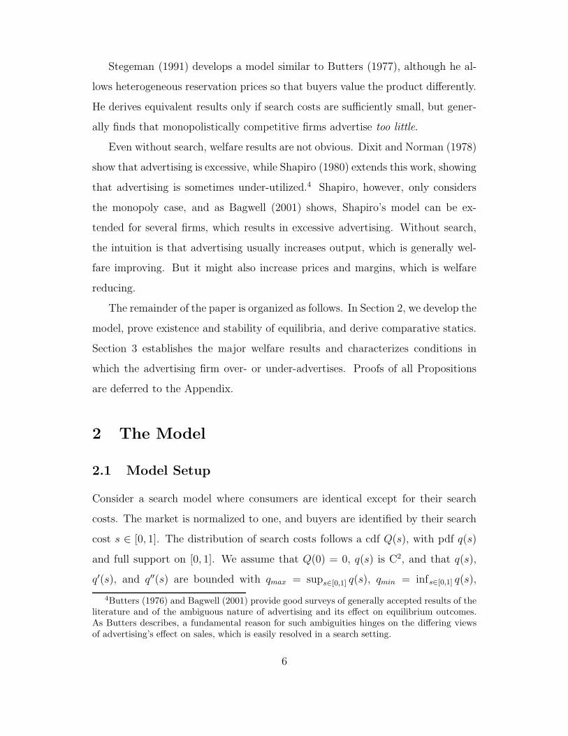
game with prices and advertising as strategic variables. Figure 1 summarizes the
setup thus far.
Figure 1: Consumer and Firm Interaction
Consumers enter themarket.
The low price firmadvertises to some x
fraction of the market.
Uninformed consumersrandomly visit one ofthe two firms.
Informed consumersvisit the low pricefirm.
Consumers offered thelow price buy thegood.
Consumers offered thehigh price can chooseto search based ontheir search costs.
Uninformed consumerswith sufficiently lowsearch costs whorandomly selected thehigh cost firm pay theextra cost to visit thelow price firm.
The remainingconsumers at the lowcost firm buy at thelow price.
Although we formally address this issue in Section 2.2, assume for now that
each firm prices according to cost so that the low cost firm is the low price firm.
In this case, the low and high price firms face the following demands:
qL = d(pL)
[
1 −1
2f(x)(1 − Q(s))
]
; (2.2)
qH =1
2d(pH)f(x)(1 − Q(s)). (2.3)
In words, (2.3) comes from some proportion—determined by x—of consumers
being informed of the low price via advertising, leaving f(x) uninformed. Of
these, half randomly select the high cost firm. Finally, some portion Q(s) have
sufficiently low search costs so that they never pay the high price, i.e., they are
active searchers. (2.3) is therefore the probability that any given buyer purchases
8
from the high price firm, where each buyer demands d(pH) units. The remaining
consumers pay the low price and demand d(pL) units each, which yields (2.2).
2.2 Existence, Stability, and Comparative Statics
We assume the monopolist’s problem
maxp∈[0,pmax)
Π = d(p)(p − c)
has a unique solution, denoted p∗, where Πp > 0 on [0, p∗). Consumers receive
sufficient indirect utility so that they always purchase at the monopoly price (i.e.
v(p∗) + y ≥ p∗). We also assume
Πpp > −dpΠ, (2.4)
which essentially restricts the elasticity of demand. For notational convenience,
denote the monopolist’s first order condition evaluated at the high cost firm’s
price and cost by ΠHp and similarly for the low cost firm.
In this paper, we want to focus on the natural equilibrium where the low cost
firm is the low price firm. We therefore begin with an artificially restricted case
where the low cost firm must price below the high cost firm. As such, only the
low cost firm advertises and faces the profit maximization problem
maxpL≤pH
x≤1
pLqL − Ax, (2.5)
which yields the following first order conditions for price and advertising respec-
9
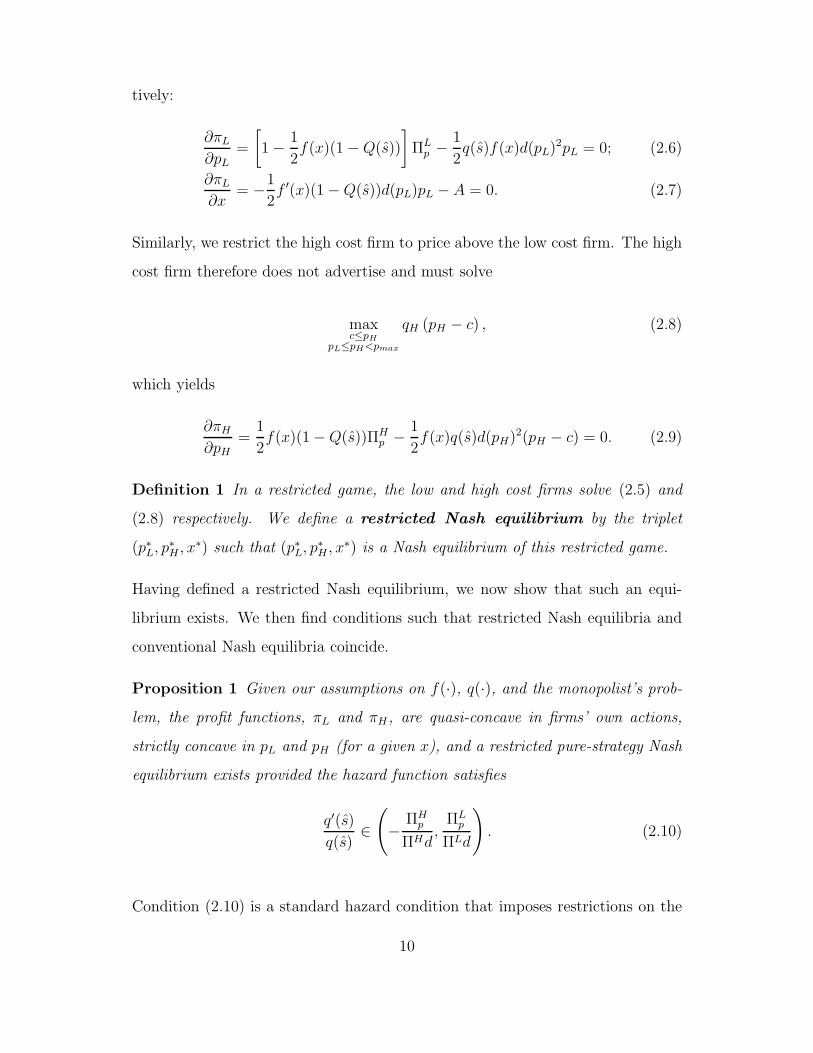
tively:
∂πL
∂pL
=
[
1 −1
2f(x)(1 − Q(s))
]
ΠLp −
1
2q(s)f(x)d(pL)2pL = 0; (2.6)
∂πL
∂x= −
1
2f ′(x)(1 − Q(s))d(pL)pL − A = 0. (2.7)
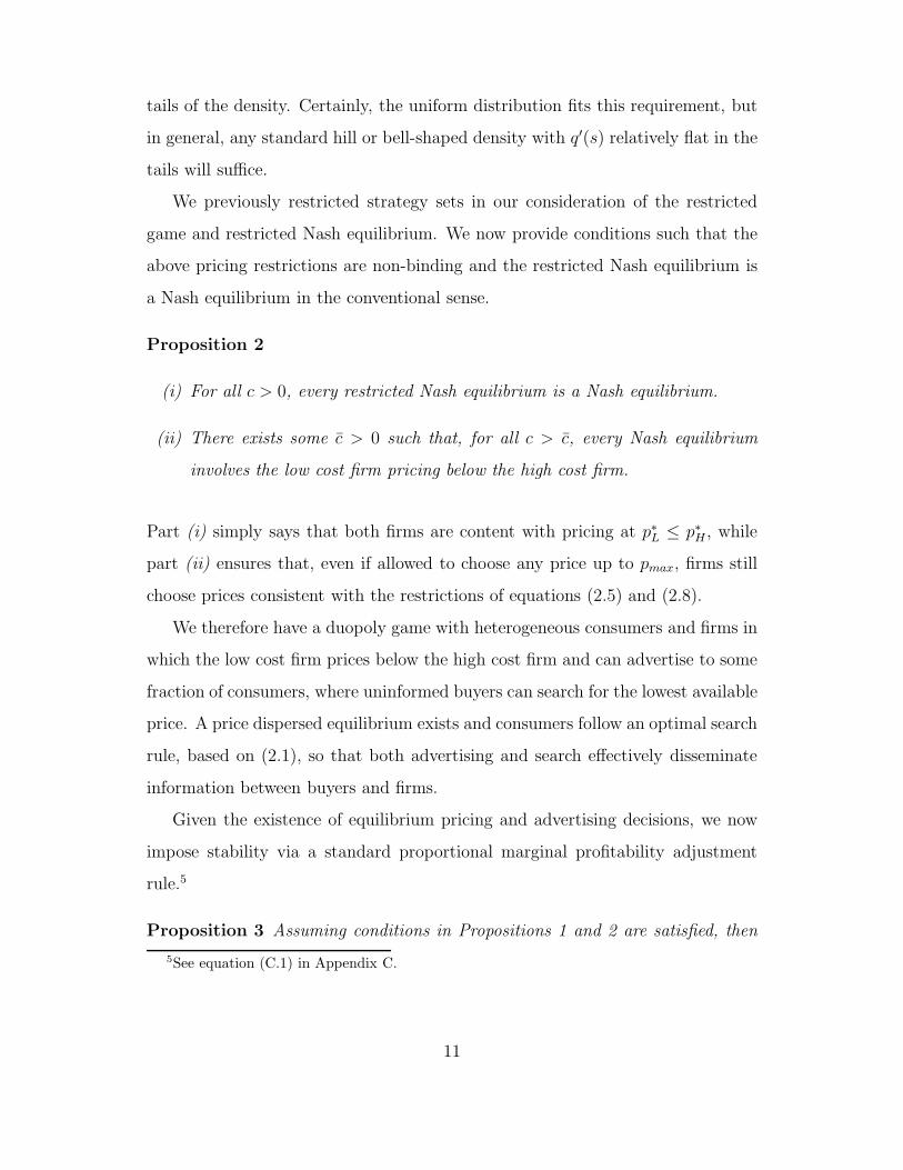
Similarly, we restrict the high cost firm to price above the low cost firm. The high
cost firm therefore does not advertise and must solve
maxc≤pH
pL≤pH<pmax
qH (pH − c) , (2.8)
which yields
∂πH
∂pH
=1
2f(x)(1 − Q(s))ΠH
p −1
2f(x)q(s)d(pH)2(pH − c) = 0. (2.9)
Definition 1 In a restricted game, the low and high cost firms solve (2.5) and
(2.8) respectively. We define a restricted Nash equilibrium by the triplet
(p∗L, p∗H , x∗) such that (p∗L, p∗H , x∗) is a Nash equilibrium of this restricted game.
Having defined a restricted Nash equilibrium, we now show that such an equi-
librium exists. We then find conditions such that restricted Nash equilibria and
conventional Nash equilibria coincide.
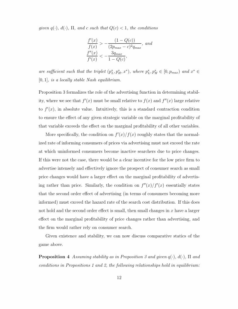
Proposition 1 Given our assumptions on f(·), q(·), and the monopolist’s prob-
lem, the profit functions, πL and πH , are quasi-concave in firms’ own actions,
strictly concave in pL and pH (for a given x), and a restricted pure-strategy Nash
equilibrium exists provided the hazard function satisfies
q′(s)
q(s)∈
(
−ΠH
p
ΠHd,
ΠLp
ΠLd
)
. (2.10)
Condition (2.10) is a standard hazard condition that imposes restrictions on the
10
tails of the density. Certainly, the uniform distribution fits this requirement, but
in general, any standard hill or bell-shaped density with q′(s) relatively flat in the
tails will suffice.
We previously restricted strategy sets in our consideration of the restricted
game and restricted Nash equilibrium. We now provide conditions such that the
above pricing restrictions are non-binding and the restricted Nash equilibrium is
a Nash equilibrium in the conventional sense.
Proposition 2
(i) For all c > 0, every restricted Nash equilibrium is a Nash equilibrium.
(ii) There exists some c > 0 such that, for all c > c, every Nash equilibrium
involves the low cost firm pricing below the high cost firm.
Part (i) simply says that both firms are content with pricing at p∗L ≤ p∗H , while
part (ii) ensures that, even if allowed to choose any price up to pmax, firms still
choose prices consistent with the restrictions of equations (2.5) and (2.8).
We therefore have a duopoly game with heterogeneous consumers and firms in
which the low cost firm prices below the high cost firm and can advertise to some
fraction of consumers, where uninformed buyers can search for the lowest available
price. A price dispersed equilibrium exists and consumers follow an optimal search
rule, based on (2.1), so that both advertising and search effectively disseminate
information between buyers and firms.
Given the existence of equilibrium pricing and advertising decisions, we now
impose stability via a standard proportional marginal profitability adjustment
rule.5
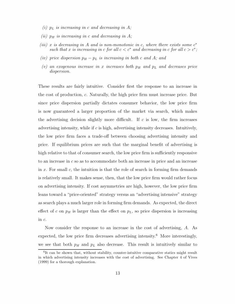
Proposition 3 Assuming conditions in Propositions 1 and 2 are satisfied, then
5See equation (C.1) in Appendix C.
11
given q(·), d(·), Π, and c such that Q(c) < 1, the conditions
f ′(x)
f(x)> −
(1 − Q(c))
(2pmax − c)2qmax
, and
f ′′(x)
f ′(x)< −
3qmax
1 − Q(c),
are sufficient such that the triplet (p∗L, p∗H , x∗), where p∗L, p∗H ∈ [0, pmax) and x∗ ∈
[0, 1], is a locally stable Nash equilibrium.
Proposition 3 formalizes the role of the advertising function in determining stabil-
ity, where we see that f ′(x) must be small relative to f(x) and f ′′(x) large relative
to f ′(x), in absolute value. Intuitively, this is a standard contraction condition
to ensure the effect of any given strategic variable on the marginal profitability of
that variable exceeds the effect on the marginal profitability of all other variables.
More specifically, the condition on f ′(x)/f(x) roughly states that the normal-
ized rate of informing consumers of prices via advertising must not exceed the rate
at which uninformed consumers become inactive searchers due to price changes.
If this were not the case, there would be a clear incentive for the low price firm to
advertise intensely and effectively ignore the prospect of consumer search as small
price changes would have a larger effect on the marginal profitability of advertis-
ing rather than price. Similarly, the condition on f ′′(x)/f ′(x) essentially states
that the second order effect of advertising (in terms of consumers becoming more
informed) must exceed the hazard rate of the search cost distribution. If this does
not hold and the second order effect is small, then small changes in x have a larger
effect on the marginal profitability of price changes rather than advertising, and
the firm would rather rely on consumer search.
Given existence and stability, we can now discuss comparative statics of the
game above.
Proposition 4 Assuming stability as in Proposition 3 and given q(·), d(·), Π and
conditions in Propositions 1 and 2, the following relationships hold in equilibrium:
12
(i) pL is increasing in c and decreasing in A;
(ii) pH is increasing in c and decreasing in A;
(iii) x is decreasing in A and is non-monotonic in c, where there exists some c∗
such that x is increasing in c for all c < c∗ and decreasing in c for all c > c∗;
(iv) price dispersion pH − pL is increasing in both c and A; and
(v) an exogenous increase in x increases both pH and pL and decreases pricedispersion.
These results are fairly intuitive. Consider first the response to an increase in
the cost of production, c. Naturally, the high price firm must increase price. But
since price dispersion partially dictates consumer behavior, the low price firm
is now guaranteed a larger proportion of the market via search, which makes
the advertising decision slightly more difficult. If c is low, the firm increases
advertising intensity, while if c is high, advertising intensity decreases. Intuitively,
the low price firm faces a trade-off between choosing advertising intensity and
price. If equilibrium prices are such that the marginal benefit of advertising is
high relative to that of consumer search, the low price firm is sufficiently responsive
to an increase in c so as to accommodate both an increase in price and an increase
in x. For small c, the intuition is that the role of search in forming firm demands
is relatively small. It makes sense, then, that the low price firm would rather focus
on advertising intensity. If cost asymmetries are high, however, the low price firm
leans toward a “price-oriented” strategy versus an “advertising intensive” strategy
as search plays a much larger role in forming firm demands. As expected, the direct
effect of c on pH is larger than the effect on pL, so price dispersion is increasing
in c.
Now consider the response to an increase in the cost of advertising, A. As
expected, the low price firm decreases advertising intensity.6 More interestingly,
we see that both pH and pL also decrease. This result is intuitively similar to
6It can be shown that, without stability, counter-intuitive comparative statics might resultin which advertising intensity increases with the cost of advertising. See Chapter 4 of Vives(1999) for a thorough explanation.
13
that above as the low price firm relies on a “price-oriented” strategy. In doing
so, the high price firm must respond with a price decrease so as to avoid losing a
large market share due to high price dispersion and subsequent consumer search.
We therefore find that, for an increase in A and perhaps c, the strategic value
of advertising decreases, and firms become more price oriented. Such behavior
highlights the important role of search in firm pricing decisions. Again, since A
has a direct effect on pL, price dispersion is increasing in A.
Condition (v) shows that, while individual prices are increasing with advertis-
ing intensity, price dispersion is decreasing. An exogenous increase in x therefore
has a larger impact on the advertising firm than on the high price firm. This de-
crease in price dispersion subsequently decreases the proportion of consumers who
engage in search. As we will see in Section 3, this tradeoff between advertising
and search intensity has important welfare implications.
3 Welfare and Advertising Intensity
We now have a model in which advertising plays a purely informational role in
announcing the true price and location of the low cost firm, and thus implicitly
doing so for the high cost firm. But as mentioned in Section 1, welfare effects are
unclear due to the inherent tension between the social planner and the advertising
firm. The planner knows it is socially optimal that consumers reach the low cost
firm on their first attempt, rather than pay additional search costs, but does not
account for firm profits. The low cost firm, however, cares only about profit and is
indifferent to whatever search costs its customers accrue. Our goal now, therefore,
is to fully characterize when and how this tension might lead the firm to over- or
under-advertising relative to a planner.
Formally, we consider the basic pricing/advertising game proposed in Section 2
and study the duopolistic advertising level relative to the level chosen by a social
planner. For simplification, we assume all consumers inelastically demand one
14
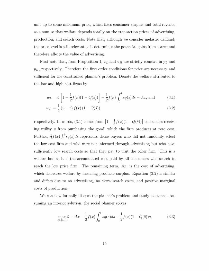
unit up to some maximum price, which fixes consumer surplus and total revenue
as a sum so that welfare depends totally on the transaction prices of advertising,
production, and search costs. Note that, although we consider inelastic demand,
the price level is still relevant as it determines the potential gains from search and
therefore affects the value of advertising.
First note that, from Proposition 1, πL and πH are strictly concave in pL and
pH , respectively. Therefore the first order conditions for price are necessary and
sufficient for the constrained planner’s problem. Denote the welfare attributed to
the low and high cost firms by
wL = u
[
1 −1
2f(x)(1 − Q(s))
]
−1
2f(x)
∫ s
0
sq(s)ds − Ax, and (3.1)
wH =1
2(u − c) f(x) (1 − Q(s)) (3.2)
respectively. In words, (3.1) comes from[
1 − 12f(x)(1 − Q(s))
]
consumers receiv-
ing utility u from purchasing the good, which the firm produces at zero cost.
Further, 12f(x)
∫ s
0sq(s)ds represents those buyers who did not randomly select
the low cost firm and who were not informed through advertising but who have
sufficiently low search costs so that they pay to visit the other firm. This is a
welfare loss as it is the accumulated cost paid by all consumers who search to
reach the low price firm. The remaining term, Ax, is the cost of advertising,
which decreases welfare by lessening producer surplus. Equation (3.2) is similar
and differs due to no advertising, no extra search costs, and positive marginal
costs of production.
We can now formally discuss the planner’s problem and study existence. As-
suming an interior solution, the social planner solves
maxx∈[0,1]
u − Ax −1
2f(x)
∫ s
0
sq(s)ds −1
2f(x)(1 − Q(s))c, (3.3)
15
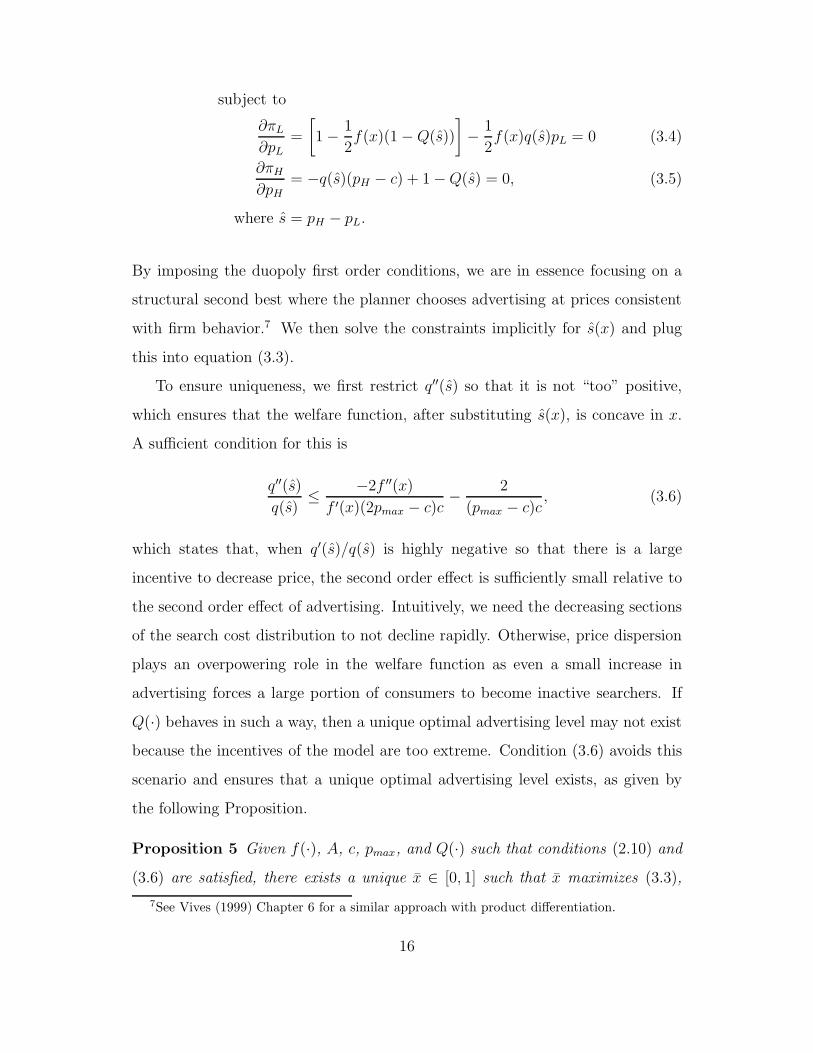
subject to
∂πL
∂pL
=
[
1 −1
2f(x)(1 − Q(s))
]
−1
2f(x)q(s)pL = 0 (3.4)
∂πH
∂pH
= −q(s)(pH − c) + 1 − Q(s) = 0, (3.5)
where s = pH − pL.
By imposing the duopoly first order conditions, we are in essence focusing on a
structural second best where the planner chooses advertising at prices consistent
with firm behavior.7 We then solve the constraints implicitly for s(x) and plug
this into equation (3.3).
To ensure uniqueness, we first restrict q′′(s) so that it is not “too” positive,
which ensures that the welfare function, after substituting s(x), is concave in x.
A sufficient condition for this is
q′′(s)
q(s)≤
−2f ′′(x)
f ′(x)(2pmax − c)c−
2
(pmax − c)c, (3.6)
which states that, when q′(s)/q(s) is highly negative so that there is a large
incentive to decrease price, the second order effect is sufficiently small relative to
the second order effect of advertising. Intuitively, we need the decreasing sections
of the search cost distribution to not decline rapidly. Otherwise, price dispersion
plays an overpowering role in the welfare function as even a small increase in
advertising forces a large portion of consumers to become inactive searchers. If
Q(·) behaves in such a way, then a unique optimal advertising level may not exist
because the incentives of the model are too extreme. Condition (3.6) avoids this
scenario and ensures that a unique optimal advertising level exists, as given by
the following Proposition.
Proposition 5 Given f(·), A, c, pmax, and Q(·) such that conditions (2.10) and
(3.6) are satisfied, there exists a unique x ∈ [0, 1] such that x maximizes (3.3),
7See Vives (1999) Chapter 6 for a similar approach with product differentiation.
16
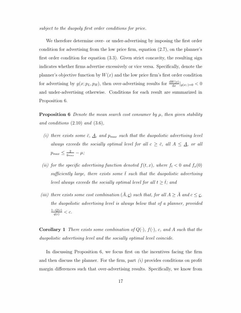
subject to the duopoly first order conditions for price.
We therefore determine over- or under-advertising by imposing the first order
condition for advertising from the low price firm, equation (2.7), on the planner’s
first order condition for equation (3.3). Given strict concavity, the resulting sign
indicates whether firms advertise excessively or vice versa. Specifically, denote the
planner’s objective function by W (x) and the low price firm’s first order condition
for advertising by g(x; pL, pH), then over-advertising results for dW (x)dx
|g(x;·)=0 < 0
and under-advertising otherwise. Conditions for each result are summarized in
Proposition 6.
Proposition 6 Denote the mean search cost consumer by µ, then given stability
and conditions (2.10) and (3.6),
(i) there exists some c, A, and pmax such that the duopolistic advertising level
always exceeds the socially optimal level for all c ≥ c, all A ≤ A, or all
pmax ≤ 2qmax
− µ;
(ii) for the specific advertising function denoted f(t, x), where ft < 0 and fx(0)
sufficiently large, there exists some t such that the duopolistic advertising
level always exceeds the socially optimal level for all t ≥ t; and
(iii) there exists some cost combination (A, c) such that, for all A ≥ A and c ≤ c,
the duopolistic advertising level is always below that of a planner, provided
1−Q(c)q(c)
< c.
Corollary 1 There exists some combination of Q(·), f(·), c, and A such that the
duopolistic advertising level and the socially optimal level coincide.
In discussing Proposition 6, we focus first on the incentives facing the firm
and then discuss the planner. For the firm, part (i) provides conditions on profit
margin differences such that over-advertising results. Specifically, we know from
17
Proposition 4 that price dispersion is increasing in c at a slower rate than c and
that advertising intensity and prices are decreasing in A. Small A or large c
therefore imply that profit margins are sufficiently different, i.e., pH − c − pL
is sufficiently large. This describes a situation in which the low cost firm has
significant leverage over its rival firm.
Large margin differences also imply that s is small relative to c so that the
indifferent consumer has a relatively low search cost. Since the firm only uses
advertising to attract high search cost buyers, it makes sense that with more high
search cost consumers in the market, the low cost firm over-advertises. This is
strongly due to the impact of advertising on consumer behavior. In essence, buyers
respond heavily to advertising because they do not care about price dispersion
and instead only care about finding a price lower than what they might otherwise
pay. In a duopoly, this implies consumers do not care how low pL is compared to
pH , just so long as pL < pH . This intuition also holds in a more general context.
For instance, with more firms so that price dispersion perhaps arises out of mixed
strategies over a particular support, an analogous interpretation is that consumers
do not care how wide the support may be, just so long as advertised prices are
below the expected price prior to search.
Note that, due to the non-monotonic nature of x with regard to changes in c,
costs of production need not be excessively high in order to satisfy “sufficiently
large.” As seen in Appendix F, over-advertising occurs when either (s−c) is highly
negative or when the duopolistic advertising level is already high so that f(x) is
small. Due to the non-monotonicity in c, advertising intensity is increasing in c
when (s − c) is close to zero and decreasing in c when (s − c) is highly negative.
Therefore, when one condition is not satisfied, the other is more likely so that
over-advertising results for a larger range of c.
Now consider the condition on pmax. If pmax is sufficiently low, the difference in
margins as well as the degree of price dispersion itself is irrelevant. The marginal
social benefit of a lower price always exceeds the firm’s marginal benefit of ad-
18
vertising. This is not an unnecessarily strong restriction as µ is always less than
one and could be much smaller. Intuitively, over-advertising results here because
price dispersion is naturally very low, implying that almost any strategy forcing
a decrease in price dispersion is excessive.
Part (i) therefore describes two different scenarios in which duopolies over-
advertise: one in which profit margins are sufficiently different so that the low
price firm has more leverage, and another in which price dispersion is more or
less restrained by the maximum willingness to pay. In the former, advertising
has a clear social benefit but is overused by firms, while in the latter, advertising
is far less beneficial. But we are also interested in how the overall shape of the
advertising function might affect welfare.
Part (ii) formally describes an advertising function where, for given amounts
of advertising, only a small share of the market remains uninformed. We see
that, without regard to price dispersion, cost asymmetries, or even search costs,
if advertising is sufficiently effective, the low price firm always takes excessive
advantage. Although more direct, this result coincides with our intuition for part
(i).
We now turn to under-advertising as discussed in part (iii). In this case,
advertising is prohibitively expensive for the firm (as given by A ≥ A) and profit
margins are sufficiently close (i.e., c ≤ c). These conditions work together to
dull the advertising incentives of the firm, so much that the firm under-advertises
relative to a planner. The requirement that 1−Q(c)q(c)
< c is essentially a hazard rate
condition that places an upper bound on the high cost firm’s profit margin even
for high price dispersion. This ensures that even if profit margins are identical, the
social benefit of advertising due to decreased expenditures on costs of production
exceeds the private benefit of advertising from attracting more high search cost
consumers.
Having discussed the incentives of the firm, we now consider those of the
planner. The key here is that changes in advertising have a uniform effect on
19
the market, while changes in price dispersion only affect consumers with search
costs in a particular range. In certain cases, the uniform effect of a marginal
change in advertising has a larger impact on the average search cost consumer,
to whom the planner is concerned, than on high search cost consumers, to whom
the advertising firm is concerned. More specifically, over- or under-advertising
depends on the share of high search cost consumers in the market as this share
determines the effect of advertising relative to search, where the planner would
rather prohibit search if the indifferent consumer has a high search cost (s > µ)
and would be more willing to allow search otherwise.
For instance, if advertising is expensive and costs of production are low, then
margins differences are small and s must be close to c. In this case, an increase
in x would decrease s so that a marginal proportion of relatively high search
cost consumers no longer pay their search cost. This proportion of newly-inactive
searchers, however, might now have to fund the cost of production c because,
due to the uniform effect of advertising, there is no guarantee that the extra
advertising would reach these same consumers. But to the planner, this tradeoff
is relatively meaningless since s and c are close. More generally, the social benefit
of advertising due to decreased search cost expenditures is high since s is relatively
high. It follows, then, that the firm under-advertises relative to a planner.
This intuition also applies when firms over-advertise. For large margin dif-
ferences, consumer search is only a small determinant of firm demand, and the
indifferent consumer has a low search cost relative to c. In this case, (i) the uni-
form effect of a change in advertising has a potentially large effect on firm demand
relative to search, and (ii) only a small portion of (low search cost) consumers
actually pay the search cost to visit the low price firm. Similar to the example
above, an increase in x would decrease s, making a marginal proportion of low
search cost consumers inactive searchers. But there is again no guarantee that the
extra advertising would reach that portion of the market. In essence, an increase
in x risks sending low search cost consumers away from the low price firm (only
20
a small social gain due to decreased search costs) and forcing them to fund the
relatively high costs of production. In this case, the planner would rather use
search to send more relatively low search cost buyers to the low price firm than
rely on the uniform effects of advertising, in which case the firm over-advertises.
Note that, for symmetric search cost distributions, the indifferent consumer
having a high search cost is equivalent to a market composed primarily of active
searchers. For such distributions, we therefore conclude that firms over-advertise
when inactive searchers compose the majority of the market and vice versa for
active searchers. This does not hold for all distributions, however, as a highly
skewed q(·) could imply a large proportion of consumers search while the indiffer-
ent consumer’s search cost remains small.
Finally, since all functions are continuous, and since both under- or over-
advertising can result, there must be some combination of distributions, functional
form specifications, and cost parameters such that the interests of both the firm
and the planner align. Although this is a knife-edge situation, it is interesting in
that the two firms, acting purely in self-interest, could reach the socially optimal
outcome.
4 Conclusion
The imperfect nature of price information in search models provides a natural
framework within which to study price advertising. Previous studies, however,
have not offered definitive welfare results under optimal consumer and firm behav-
ior. This is a nontrivial issue as the planner and firm have potentially conflicting
definitions of the value of advertising. In this paper, we put enough structure on
the market to explicitly compare optimal and duopolistic advertising levels. We
do so in an equilibrium search setting where we impose the duopolistic price level
on the planner’s problem. Our analysis explains well the relationship between the
firm’s and the planner’s incentives to advertise.
21
We find that firms might under- or over-advertise relative to a planner and that
the result depends on several factors—primarily the effectiveness of advertising
and the costs of production. Specifically, we find that firms place significantly
more weight on the informational role of advertising whenever profit margins are
sufficiently different. This means that when production cost asymmetries are large
so that the social and private values of advertising are high, it is the firm, not
the planner, that takes advantage. Conversely, we find that firms under-advertise
when advertising costs are high and margins are close and subsequently place too
much weight on the role of search in attracting buyers.
In particular, we get both under- and over-advertising in a setting where ad-
vertising is purely informative and without focusing on many identical firms. We
do so in the context of an equilibrium consumer search model where (i) advertis-
ing has an obvious role in forming and improving buyers’ knowledge of prices and
(ii) where advertising and search are imperfect substitutes for transmitting price
information. Our approach shows that the welfare effects of advertising are not a
strict byproduct of the type of advertising in question, the elasticity of demand,
or the nature of competition among firms.
22
A Proof of Proposition 1
By assumption, all functions are continuous and strategy sets are compact intervals. Therefore,by the standard Nash-Debreu theorem, a restricted pure-strategy Nash equilibrium exists solong as profit functions are quasi-concave in own strategy variables. From (2.9),
∂2πH
∂p2H
=1
2f(x)(1 − Q(s))ΠH
pp −1
2f(x)d(pH)
[
q(s)ΠHp + q′(s)d(pH)ΠH
]
−1
2f(x)q(s)
[
d(pH)ΠHp + d′(pH)ΠH
]
. (A.1)
By previous assumptions on the monopolists problem, the hazard condition, and on the ad-vertising function, we know that (A.1) is negative, so πH is strictly concave. By these sameconditions,
∂2πL
∂pL∂x= −
1
2f ′(x)
[
(1 − Q(s))ΠLp + q(s)d(pL)ΠL
]
> 0, (A.2)
∂2πL
∂x2= −
1
2f ′′(x)(1 − Q(s))d(pL)pL ≤ 0, and (A.3)
∂2πL
∂p2L
=
[
1 −1
2f(x)(1 − Q(s))
]
ΠLpp
−1
2f(x)d(pL)
[
q(s)ΠLp − q′(s)d(pL)ΠL
]
−1
2q(s)f(x)
[
d(pL)ΠLp + d′(pL)ΠL
]
< 0. (A.4)
Therefore, the determinant of the bordered Hessian for the low cost firm must be positive, whichthen implies that πL is quasi-concave.
B Proof of Proposition 2
First Prove (i)First note that, from Π = d(p)(p − c), we know that for any common price pH = pL = p,ΠH
p |pH=p = d′(p)(p − c) + d(p) > d′(p)p + d(p) = ΠLp |pL=p for all c > 0. Now suppose there
exists a restricted Nash equilibrium that is not a Nash equilibrium. In such a case, at leastone player is not making a best response. Figure 2 represents a graphical example of such asituation, where at least one firm would like to deviate from the restricted pricing strategy fora given advertising intensity x.
23
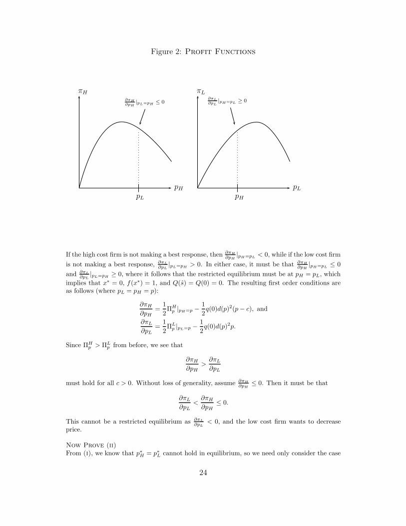
Figure 2: Profit Functions
pH pL
πH πL
pL pH
∂πH
∂pH
|pL=pH≤ 0
∂πL
∂pL
|pH=pL≥ 0
If the high cost firm is not making a best response, then ∂πH
∂pH
|pH=pL< 0, while if the low cost firm
is not making a best response, ∂πL
∂pL|pL=pH
> 0. In either case, it must be that ∂πH
∂pH|pH=pL
≤ 0
and ∂πL
∂pL
|pL=pH≥ 0, where it follows that the restricted equilibrium must be at pH = pL, which
implies that x∗ = 0, f(x∗) = 1, and Q(s) = Q(0) = 0. The resulting first order conditions areas follows (where pL = pH = p):
∂πH
∂pH
=1
2ΠH
p |pH=p −1
2q(0)d(p)2(p − c), and
∂πL
∂pL
=1
2ΠL
p |pL=p −1
2q(0)d(p)2p.
Since ΠHp > ΠL
p from before, we see that
∂πH
∂pH
>∂πL
∂pL
must hold for all c > 0. Without loss of generality, assume ∂πH
∂pH≤ 0. Then it must be that
∂πL
∂pL
<∂πH
∂pH
≤ 0.
This cannot be a restricted equilibrium as ∂πL
∂pL
< 0, and the low cost firm wants to decreaseprice.
Now Prove (ii)From (i), we know that p∗H = p∗L cannot hold in equilibrium, so we need only consider the case
24
where p∗H < p∗L. Denote each firm’s monopoly price by pM (c) = max(p − c)d(p), so that pM (0)is the monopoly price of the low cost firm. In any Nash equilibrium, p∗L < pM (0) < pmax. Thenfor pmax > c > pM (0), the high cost firm never prices below pL. Accordingly, there exists somec > 0, c < pmax, such that, for all c > c, every Nash equilibrium involves the low cost firmpricing below the high cost firm.
C Proof of Proposition 3
Assume that firms adjust their strategies according to
dai
dt= ki
∂πi(a1, a2, a3)
∂ai
(C.1)
in a neighborhood of the equilibrium. In the usual way, we take a first-order Taylor approxima-tion and, ignoring the constants ki, we find
dpL
dtdpH
dtdxdt
=
∂2πL(p∗
L,p∗
H,x∗)
∂p2
L
∂2πL(p∗
L,p∗
H,x∗)
∂pL∂pH
∂2πL(p∗
L,p∗
H,x∗)
∂pL∂x
∂2πH(p∗
L,p∗
H,x∗)
∂pH∂pL
∂2πH(p∗
L,p∗
H,x∗)
∂p2
H
∂2πH(p∗
L,p∗
H,x∗)
∂pH∂x
∂2πL(p∗
L,p∗
H,x∗)
∂x∂pL
∂2πL(p∗
L,p∗
H,x∗)
∂x∂pH
∂2πL(p∗
L,p∗
H,x∗)
∂x2
pL − p∗LpH − p∗Hx − x∗
.
We need to show that the real parts of all eigenvalues are negative, which will ensure thatour system is stable. A sufficient condition, therefore, is that our Hessian matrix has a dominantdiagonal. By definition, any n×n matrix A has a dominant diagonal if there exists some di > 0,for i = 1, 2, ..., n, such that di|πii| >
∑
j 6=i dj |πij |.For convenience, denote the following
λ11 = (A.4),
λ12 =1
2f(x)d(pH)
[
q(s)ΠLp − q′(s)d(pL)ΠL
]
,
λ13 = (A.2),
λ21 =1
2f(x)d(pL)
[
q(s)ΠHp + q′(s)d(pH)ΠH
]
,
λ22 = (A.1),
λ23 =1
2f ′(x)
[
(1 − Q(s))ΠHp − q(s)d(pH)ΠH
]
,
λ31 = (A.2),
λ32 =1
2f ′(x)q(s)d(pH)ΠH , and
λ33 = (A.3).
Denote the matrix with the above elements by Λ. Sufficient conditions under elastic demandare complicated and omitted for space. It can be shown, however, that such conditions aremaximized under inelastic demand. Accordingly, we consider unit inelastic demand to showthat Λ has a dominant diagonal. After imposing the first order conditions for price and settingd1 = d2 = d3 = 1, the following three conditions are sufficient for a dominant diagonal and thus
25
stability:
−1
2f(x)q(s) −
f ′(x)
f(x)< 0,
−1
2f(x)q(s) < 0, and
−1
2f ′′(x)(1 − Q(s))pL −
f ′(x)
f(x)−
1
2f ′(x)q(s)pL < 0.
These hold so long as
f ′(x)
f(x)> −
1
2f(x)q(s), and (C.2)
f ′′(x)
f ′(x)< −
1
1 − Q(s)
[
2
pLf(x)+ q(s)
]
. (C.3)
Using equilibrium conditions
pL =2
f(x)q(s)−
1 − Q(s)
q(s), and
pH − c =1 − Q(s)
q(s),
we see that s = 2q(s)
[
1 − Q(s) − 1f(x)
]
+ c, which implies that s is bounded above by c. We also
see that f(x) is bounded below by 2(2pmax−c)qmax
and that q(s) is bounded below by 1−Q(s)pmax−c
.
Therefore, assuming Q(c) < 1 provides an upper bound of Q(s) and a lower bound on 1−Q(s),and we can rewrite the above conditions as
f ′(x)
f(x)> −
(1 − Q(c))
(2pmax − c)(pmax − c)qmax
, and (C.4)
f ′′(x)
f ′(x)< −
3qmax
1 − Q(c). (C.5)
Therefore, under conditions (C.4) and (C.5), Λ has a dominant diagonal, and the adjustmentprocess defined by (C.1) is locally stable. Note that the expression for (C.4) given in the text isa slightly stronger sufficient condition.
D Proof of Proposition 4
Totally differentiating the system of first order conditions formed by (2.6), (2.9), and (2.7) withrespect to pL, pH , x, A, and c provides the system of equations with which to derive comparativestatics. Recalling Λ above, the differentiated system can then be written as follows:
Λ
dpL
dpH
dx
=
0− 1
2f(x)q(s)d(pH)2dc
dA
.
Just as in Appendix C, we impose the first order conditions for price, which greatly simplifiesλ23 and λ13. We also again consider the inelastic demand case for brevity, where it can be shown
26
that the determinant is maximized under this setting. This yields
|Λ| = −1
8f ′′(x)f(x)2(1 − Q(s))pL (2q(s) − q′(s)pL) (2q(s) + q′(s)(pH − c))
+1
8f ′′(x)f(x)2(1 − Q(s))pL (q(s) + q′(s)(pH − c)) (q(s) − q′(s)pL)
−f ′(x)2
2f(x)[f(x)q(s)pL (q(s) + q′(s)(pH − c)) − (2q(s) + q′(s)(pH − c))] .
Imposing stability conditions (C.2) and (C.3), it follows that |Λ| < 0, and applying Cramer’srule, we find
dpL
dc=
12f(x)q(s)
[
− 14f(x)f ′′(x)(1 − Q(s))pL[q(s) − q′(s)pL] + f ′(x)2
2f(x) q(s)pL
]
|Λ|≥ 0,
dpL
dA= −
12f ′(x) [2q(s) + q′(s)(pH − c)]
|Λ|≤ 0,
dpH
dc= −
12f(x)q(s)
[
14f ′′(x)f(x)(1 − Q(s))pL[2q(s) − q′(s)pL] − f ′(x)2
f(x)2
]
|Λ|≥ 0,
dpH
dA= −
12f ′(x)[q(s) + q′(s)(pH − c)]
|Λ|≤ 0,
dx
dc=
14f ′(x)f(x)q(s)
[
− 12f(x)q(s)pL[2q(s) − q′(s)pL] + (q(s) − q′(s)pL)
]
|Λ|
<=>
0,
dx
dA=
14f(x)2 [(2q(s) − q′(s)pL)(2q(s) + q′(s)(pH − c))]
|Λ|
−14f(x)2 [(q(s) − q′(s)pL)(q(s) + q′(s)(pH − c))]
|Λ|≤ 0.
With respect to advertising, we treat x as exogenous and derive dsdx
in the usual way. Againlooking at the inelastic demand case, totally differentiating (2.6) and (2.9) with respect to pH ,pL, x, and c yields the following system
[
−q′(s)(pH − c) − 2q(s) q′(s)(pH − c) + q(s)12f(x) (q(s) − q′(s)pL) − 1
2f(x) (2q(s) − q′(s)pL)
] [
dpH
dpL
]
=
[
−q(s)dc12f ′(x) (1 − Q(s) + q(s)pL) dx
]
.
For simplicity, define the following matrices:
Ω =
[
−q′(s)(pH − c) − 2q(s) q′(s)(pH − c) + q(s)12f(x) (q(s) − q′(s)pL) − 1
2f(x) (2q(s) − q′(s)pL)
]
,
ΩpH=
[
−q(s)dc q′(s)(pH − c) + q(s)12f ′(x) (1 − Q(s) + q′(s)pL) dx − 1
2f(x) (2q(s) − q′(s)pL)
]
, and
ΩpL=
[
−q′(s)(pH − c) − 2q(s) −q(s)dc12f(x) (q(s) − q′(s)pL) 1
2f ′(x) (1 − Q(s) + q′(s)pL) dx
]
.
From conditions (2.10) and (A.1), we know that
|Ω| =1
2f(x)q(s) [q′(s)(pH − pL − c) + 3q(s)] > 0.
27
Looking only at pH , we see that
dpH =[2q(s) − q′(s)pL] dc
q′(s)(pH − pL − c) + 3q(s)
−f ′(x) [1 − Q(s) + q(s)pL] [q′(s)(pH − c) + q(s)] dx
f(x)q(s) [q′(s)(pH − pL − c) + 3q(s)].
Setting dc to zero, we find
dpH
dx=
−f ′(x) [1 − Q(s) + q(s)pL] [q′(s)(pH − c) + q(s)]
f(x)q(s) [q′(s)(pH − pL − c) + 3q(s)].
The same process for pL yields
dpL
dx=
−f ′(x) [1 − Q(s) + q(s)pL] [q′(s)(pH − c) + 2q(s)]
f(x)q(s) [q′(s)(pH − pL − c) + 3q(s)].
Therefore, we know
ds
dx=
dpH
dx−
dpL
dx=
f ′(x) [1 − Q(s) + q(s)pL]
f(x) [q′(s)(pH − pL − c) + 3q(s)]< 0.
E Proof of Proposition 5
Since πL and πH are concave in pL and pH respectively, the first order conditions for pL and pH
are necessary and sufficient for a constrained optimum of the planner’s problem. We can thensolve the constraints implicitly for s(x) and plug this into the objective function. To ensure aunique optimum, we need only show that the resulting function is strictly concave.
Differentiating the welfare function and rearranging terms yields
d2W
dx2= −
1
2f ′′(x)
[
(1 − Q(s))c +
∫ s
0
sq(s)ds
]
− f ′(x)q(s)(s − c)ds
dx−
1
2f(x)q(s)
(
ds
dx
)2
−1
2f(x)(s − c)
[
q′(s)
(
ds
dx
)2
+ q(s)d2s
dx2
]
. (E.1)
After substituting dsdx
and d2 sdx2 and some tedious algebra, we see that (E.1) is always negative pro-
vided q′′(s)q(s) ≤ −f ′′(x)
f ′(x)(2pmax−c)c −2
(pmax−c)c , and there exists a unique socially optimal advertising
level subject to the equilibrium duopoly price level.
F Proof of Proposition 6
First Prove (i)
For convenience, denote φ =∫ s
0sq(s)ds + (1 − Q(s))(c − pL), then substituting the firm’s first
28
order condition for advertising, (2.7), yields
dW
dx|xd = −
1
2f ′(x)φ −
1
2f(x)q(s)(s − c)
ds
dx
= −1
2f ′(x)φ −
1
2f ′(x)q(s)(s − c)
1 − Q(s) + q(s)pL
q′(s)(pH − pL − c) + 3q(s)
= −1
2f ′(x)φ − q(s)
f ′(x)(s − c)
f(x) [q′(s)(pH − pL − c) + 3q(s)]
where the third equality comes from substituting (2.6). From this equation, we know the signof dW
dx|xd depends on φ. To see this, note that equilibrium first order conditions, (2.6) and (2.9),
require
s − c = pH − pL − c =2
q(s)
[
1 − Q(s) − f−1(x)]
which is nonpositive as f(x) ∈ [0, 1] and Q(s) ≥ 0. Also, from (2.10) we know q′(s)(pH − pL −c) + 3q(s) > 0. So the following results hold:
dW
dx|xd > 0 iff φ >
−2q(s)(s − c)
f(x) [q′(s)(s − c) + 3q(s)]; (F.1)
dW
dx|xd ≤ 0 iff φ ≤
−2q(s)(s − c)
f(x) [q′(s)(s − c) + 3q(s)]. (F.2)
We proceed by examining the comparative statics of s to changes in c and A as well the upperbound of φ to determine when equation (F.2) holds.
First consider the upper bound of φ. From equations (2.6) and (2.9), we see that c − pL =pH − 2
q(s)f(x) , which is bounded above by pmax − 2qmax
. This implies that φ is bounded above
by µ + pmax − 2qmax
, where µ is the mean of s (note that µ ≥∫ s
0 sq(s)ds). Therefore, for
pmax < 2qmax
− µ, it follows that dWdx
|xd ≤ 0.Now consider comparative statics. First, we rewrite the upper bound of φ by noting that
∫ s
0 sq(s)ds ≤ sQ(s), which implies that φ ≤ c + Q(s)(s − c). Therefore, over-advertising resultsfor
c + Q(s)(s − c) ≤ −2(s − c)
f(x)[
q′(s)q(s) (s − c) + 3
] . (F.3)
We use both equations (F.2) and (F.3) in the following. Note that any equilibrium requiress ≤ 1. Otherwise, the low price firm could increase price to pH − 1 and still get the entiremarket. Since s− c is always negative in equilibrium, this implies that min1, c ≥ s ≥ 0. Nowconsider the left and right hand sides of equation (F.2) as s goes to its maximum, where wesee that the left hand side is bounded above by c for c < 1 and bounded above by µ for c > 1,and the right hand side is equal to 0 for c < 1 and is positive for c > 1. For the lower boundof s (s = 0), we see that φ = c − pH < 0 as s = 0 ⇒ pL = pH . Since the right hand side ispositive for s = 0, it follows that equation (F.2) is always satisfied for s = 0 and unsatisfied fors = c < 1. Figure 3 describes these bounds graphically, where over-advertising is depicted bythe range in which RHS is above LHS. We only consider graphically the case where c < 1, buta similar result holds for c > 1 as φ remains bounded above by µ.
29
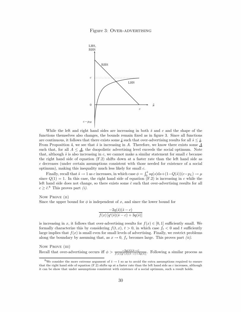
Figure 3: Over-advertising
s
LHS,RHS
c
c
c−pH
0
LHS
RHS
While the left and right hand sides are increasing in both s and c and the shape of thefunctions themselves also changes, the bounds remain fixed as in figure 3. Since all functionsare continuous, it follows that there exists some s such that over-advertising results for all s ≤ s.From Proposition 4, we see that s is increasing in A. Therefore, we know there exists some A
such that, for all A ≤ A, the duopolistic advertising level exceeds the social optimum. Notethat, although s is also increasing in c, we cannot make a similar statement for small c becausethe right hand side of equation (F.2) shifts down at a faster rate than the left hand side asc decreases (under certain assumptions consistent with those needed for existence of a socialoptimum), making this inequality much less likely for small c.
Finally, recall that s → 1 as c increases, in which case φ =∫ s
0 sq(s)ds+(1−Q(s))(c−pL) → µ
since Q(1) = 1. In this case, the right hand side of equation (F.2) is increasing in c while theleft hand side does not change, so there exists some c such that over-advertising results for allc ≥ c.8 This proves part (i).
Now Prove (ii)Since the upper bound for φ is independent of x, and since the lower bound for
−2q(s)(s − c)
f(x) [q′(s)(s − c) + 3q(s)]
is increasing in x, it follows that over-advertising results for f(x) ∈ [0, 1] sufficiently small. Weformally characterize this by considering f(t, x), t > 0, in which case ft < 0 and t sufficientlylarge implies that f(x) is small even for small levels of advertising. Finally, we restrict problemsalong the boundary by assuming that, as x → 0, fx becomes large. This proves part (ii).
Now Prove (iii)
Recall that over-advertising occurs iff φ >−2q(s)(s−c)
f(x)[q′(s)(s−c)+3q(s)] . Following a similar process as
8We consider the more extreme argument of s → 1 so as to avoid the extra assumptions required to ensurethat the right hand side of equation (F.2) shifts up at a faster rate than the left hand side as c increases, althoughit can be show that under assumptions consistent with existence of a social optimum, such a result holds.
30
with part (i), s → c as A increases, which implies that pH − c = pL. This also implies that(1 − Q(s))(c − pL) → (1 − Q(c))(c − (pH − c)) as s → c.
Now consider (1 − Q(c))(2c − pH) as a lower bound for φ at s = c. To ensure that this is
positive, we need 1−Q(c)q(c) < c, in which case φ is positive at this lower bound and the right hand
side goes to zero. Therefore, provided c is relatively small, equation (F.1) will hold for some A
sufficiently large since s is increasing in A. So, there exists some cost pair (A, c) such that forall A ≥ A and c ≤ c the duopolistic advertising level is below that of a planner. This provespart (iii).
G Proof of Corollary
Since the welfare function is continuous in all variables and strictly concave in x, and since theproof for Proposition 6 shows that it is possible for both dW
dx|xd > 0 and dW
dx|xd ≤ 0 depending
on functional and parameter specifics, it follows that there is some intermediate value of x suchthat dW
dx|xd = 0. By strict concavity, this advertising level must be such that the duopolistic
and socially optimal advertising levels are the same.
31
References[1] Anderson, S. and R. Renault. (2000). “Consumer Information and Firm Pricing: Negative
Externalities from Improved Information.” International Economic Review 41, 721-42.
[2] Anderson, S. and R. Renault. (2004). “Advertising Content.” Working Paper.
[3] Bagwell, K. and G. Ramey. (1994). “Coordination Economies, Advertising, and SearchBehavior in Retail Markets.” American Economic Review 84, 498-517.
[4] Bagwell, K. (2001). “The Economic Analysis of Advertising.” Mimeo, Columbia University.
[5] Baye, M. and J. Morgan. (2001). “Information Gatekeepers on the Internet and theCompetitiveness of Homogeneous Product Markets.” American Economic Review 91,454-74.
[6] Baye, M., J. Morgan, and P. Scholten. (2006). “Information, Search, and Price Dispersion.”Handbook on Economics and Information Systems, forthcoming.
[7] Benabou, R. (1988). “Search, Price Setting and Inflation.” Review of Economic Studies 55,353-76.
[8] Benabou, R. (1993). “Search Market Equilibrium, Bilateral Heterogeneity, and RepeatPurchases.” Journal of Economic Theory 60, 140-58.
[9] Burdett, K. and K. Judd. (1983). “Equilibrium Price Dispersion.” Econometrica 51, 955-70.
[10] Butters, G. (1976). “A Survey of Advertising and Market Structure.” American EconomicReview 66, 392-97.
[11] Butters, G. (1977). “Equilibrium Distributions of Sales and Advertising Prices.” Reviewof Economic Studies 44, 465-91.
[12] Carlson, J. and P. McAfee. (1983). “Discrete Equilibrium Price Dispersion.” Journal ofPolitical Economy 91, 480-93.
[13] Dana, J. (1994). “Learning in an Equilibrium Search Model.” International EconomicReview 35, 745-71.
[14] Dixit, A. and V. Norman. (1978). “Advertising and Welfare.” Bell Journal of Economics9, 1-17.
[15] Grossman, M. and C. Shapiro. (1984). “Informative Advertising and DifferentiatedProducts.” Review of Economic Studies 51, 63-81.
[16] Janssen, M., J. Moraga-Gonzalez, and M. Wildenbeest. (2005). “Truly Costly SequentialSearch and Oligopolistic Pricing.” International Journal of Industrial Organization 23,451-66.
[17] Janssen, M., and M. Non. (2005). “Advertising and Consumer Search in a DuopolyModel.” Discussion Paper.
[18] Kihlstrom, R. and M. Riordan. (1984). “Advertising as a Signal.” Journal of PoliticalEconomy 92, 427-50.
32
[19] MacMinn, R. (1980). “Search and Market Equilibrium.” Journal of Political Economy 88,308-27.
[20] Morgan, P. and R. Manning. (1985) “Optimal Search.” Econometrica 53, 923-44.
[21] Nelson, P. (1974). “Advertising as Information.” Journal of Political Economy 82, 729-54.
[22] Nichols, L. (1985). “Advertising and Economic Welfare.” The American Economic Review75, 213-28.
[23] Rauh, M. (2004). ”Wage and Price Controls in the Equilibrium Sequential Search Model.”European Economic Review 48, 1287-1300.
[24] Reinganum, J. (1979). “A Simple Model of Equilibrium Price Dispersion.” Journal ofPolitical Economy 87, 851-58.
[25] Rob, R. (1985). “Equilibrium Price Distributions.” Review of Economic Studies 52,487-502.
[26] Robert, J. and D. Stahl. (1993). “Informative Price Advertising in a Sequential SearchModel.” Econometrica 61, 657-86.
[27] Shapiro, C. (1980). “Advertising and Welfare: Comment.” Bell Journal of Economics 11,749-52.
[28] Stahl, D. (1989). “Oligopolistic Pricing with Sequential Consumer Search.” AmericanEconomic Review 79, 700-12.
[29] Stegeman, M. (1991). “Advertising in Competitive Markets.” American Economic Review81, 210-23.
[30] Tirole, J. (1988). The Theory of Industrial Organization. MIT Press, Cambridge, MA.
[31] Vives, X. (1999). Oligopoly Pricing: Old Ideas and New Tools. MIT Press, Cambridge, MA.
33
Recommended