ADAPTIVE CAMERA TAMPER DETECTION FOR VIDEO SURVEILLANCE
A THESIS SUBMITTED TO
THE GRADUATE SCHOOL OF INFORMATICS
OF
THE MIDDLE EAST TECHNICAL UNIVERSITY
BY
ALĠ SAĞLAM
IN PARTIAL FULFILLMENT OF THE REQUIREMENTS FOR THE DEGREE OF
MASTER OF SCIENCE
IN
THE DEPARTMENT OF INFORMATION SYSTEMS
JUNE 2009

Approval of the Graduate School of Informatics
________________
Prof. Dr. Nazife Baykal
Director
I certify that this thesis satisfies all the requirements as a thesis for the degree of
Master of Science.
___________________
Prof. Dr. Yasemin Yardımcı
Head of Department
This is to certify that we have read this thesis and that in our opinion it is fully
adequate, in scope and quality, as a thesis for the degree of Master of Science.
___________________
Assist. Prof. Dr. Alptekin Temizel
Supervisor
Examining Committee Members
Prof. Dr. Yasemin Yardımcı (METU, II) _____________________
Assist. Prof. Dr. Alptekin Temizel (METU, II) _____________________
Assist. Prof. Dr. Erhan Eren (METU, II) _____________________
Dr. Sevgi Özkan (METU, II) _____________________
Assist. Prof. Dr. Ġlkay Ulusoy (METU, EE) _____________________

iii
I hereby declare that all information in this document has been obtained and
presented in accordance with academic rules and ethical conduct. I also declare
that, as required by these rules and conduct, I have fully cited and referenced
all material and results that are not original to this work.
Name, Last name : Ali Sağlam
Signature : _________________

iv
ABSTRACT
ADAPTIVE CAMERA TAMPER DETECTION FOR VIDEO
SURVEILLANCE
SAĞLAM, Ali
M.S., Department of Information Systems
Supervisor: Assist. Prof. Dr. Alptekin Temizel
June 2009, 54 pages
Criminals often resort to camera tampering to prevent capture of their actions. Many
surveillance systems left unattended and videos surveillance system operators lose their
concentration after a short period of time. Many important Real-time automated detection of
video camera tampering cases is important for timely warning of the operators. Tampering
can be defined as deliberate physical actions on a video surveillance camera and is generally
done by obstructing the camera view by a foreign object, displacing the camera and changing
the focus of the camera lens. In automated camera tamper detection systems, low false alarm
rates are important as reliability of these systems is compromised by unnecessary alarms and
consequently the operators start ignoring the warnings. We propose adaptive algorithms to
detect and identify such cases with low false alarms rates in typical surveillance scenarios
where there is significant activity in the scene. We also give brief information about the
camera tampering detection algorithms in the literature. In this thesis we compare
performance of the proposed algorithms to the algorithms in the literature by experimenting
them with a set of test videos.
Keywords: video surveillance, camera tampering, camera sabotage, covered camera,
defocused camera

v
ÖZ
VİDEO GÖZETLEME İÇİN UYARLANABİLİR KAMERA
TAHRİFİ TESBİT ETME
SAĞLAM, Ali
Yüksek Lisans, Bilişim Sistemleri
Tez Yöneticisi: Yrd. Doç. Dr. Alptekin Temizel
Haziran 2009, 54 sayfa
Suçlular, suç işlerken görüntülerinin çekilmesini önlemek amacıyla kameraları tahrif etme
yöntemine sıklıkla başvururlar. Bir çok video gözetleme sistemi gözetimsiz bırakılır ve
kamera görüntülerini izleyen operatörler kısa bir sure sonra dikkatlerini kaybederler. Kamera
tahrif edildiğinde kamera görüntülerini izleyen operatörlerin zamanında uyarılabilmesini
sağlayan gerçek zamanlı ve otomatik tesbit önemlidir. Kamera tahrifi bir video kameraya
yapılan kasıtlı fiziksel eylemler olarak tanımlanabilir ve genellikle kameranın görüşünü
yabancı bir nesne ile engelleyerek, kameranın yerini değiştirerek, kamera lensinin odağını
değiştirilerek yapılır. Kamera tahrifini otomatik belirleyen sistemlerde yanlış alarm oranının
az olması önemlidir, çünkü yanlış alarmlar sistemin güvenilirliğini düşürür ve bunun
neticesinde kamera görüntülerini izleyen operator sistemin uyarılarını göz ardı etmeye
başlar. Bu tezde içerisinde önemli ölçüde hareket olan tipik gözetleme senaryolarında
kamera tahrifini ve kamera tahrifinin ne şekilde yapıldığını tesbit etmek için uyarlanabilir
algoritmalar sunuyoruz. Ayrıca literatürdeki kamera tahrifini tesbit etmek için kullanılan
algoritmalar hakkında özet bilgi veriyoruz. Bu tezde bir test videosu kümesi ile deneyler
yaparak bizim sunduğumuz kamera tahrifini tesbit etme algoritmalarının performansını
literatürdeki diğer algoritmalar ile karşılaştırıyoruz.

vi
Anahtar Kelimeler: Video Gözetlemek, Kamera Tahrifi, Önü Kapatılmış Kamera, Odağı
Bozulmuş Kamera, Yeri Değiştirilmiş Kamera

vii
ACKNOWLEDGMENTS
I am deeply grateful to my supervisor Assist. Prof.Dr. Alptekin Temizel, who has helped me
throughout my research, and encouraged me in my academic life. He always had time to
discuss things and showed me the way when I felt lost in my research. It was a great
opportunity to work with him.
I would like to thank my colleagues at TÜBĠTAK-UEKAE/G222 Unit, for their support and
insightful comments. My sincere thanks also goes to my friends, Kadir Soydal and Selçuk
Türkel for their help in capturing the test videos.
I would also like to address my thanks to The Scientific and Technological Research Council
of Turkey (TÜBĠTAK) for its scholarship during initial stages of my MS study.
Finally, I would like to thank my family and Rahime Belen for supporting my educational
goals. Without their love, help and encouragement, this thesis has not been completed.

viii
TABLE OF CONTENTS
ABSTRACT ................................................................................................................ iv
ÖZ ................................................................................................................................ v
ACKNOWLEDGMENTS ......................................................................................... vii
TABLE OF CONTENTS .......................................................................................... viii
LIST OF TABLES ....................................................................................................... x
LIST OF FIGURES .................................................................................................... xi
LIST OF ABBREVIATIONS ................................................................................... xiv
CHAPTER
INTRODUCTION ................................................................................................... 1
BACKGROUND SUBTRACTION ........................................................................ 4
2.1 Overview ....................................................................................................... 4
2.2 Background Subtraction Methods in the Literature ...................................... 4
2.3 Background Subtraction Method of Video Surveillance And Monitoring
(VSAM) System ........................................................................................... 8
LITERATURE REVIEW ...................................................................................... 12
3.1 Overview ..................................................................................................... 12
3.2 Camera Tamper Detection Using Wavelet Analysis for Video Surveillance
.................................................................................................................... 14
3.3 Automatic Control of Video Surveillance Camera Sabotage ...................... 15
3.3 Real-Time Detection of Camera Tampering ............................................... 16
ADAPTIVE CAMERA TAMPER DETECTION ALGORITHMS ..................... 20
4.1 Overview ..................................................................................................... 20
4.2 Detection of Defocused Camera View ........................................................ 20
4.3 Detection of Moved Camera ....................................................................... 26
4.4 Detection of Covered Camera View ........................................................... 28

ix
EXPERIMENTAL RESULTS AND COMPARISONS ....................................... 32
5.1 Overview ..................................................................................................... 32
5.2 Testing Environment ................................................................................... 32
5.3 Experimental Results ................................................................................... 34
5.3.1 Defocused Camera View ...................................................................... 34
5.3.2 Moved Camera ..................................................................................... 40
5.3.3 Covered Camera View ......................................................................... 43
CONCLUSIONS AND FUTURE WORK ............................................................ 50
REFERENCES ........................................................................................................... 52

x
LIST OF TABLES
TABLE
1. Defocused Camera Test Results for Different Algorithms .................................. 34
2. Moved Camera Test Results for Different Algorithms ....................................... 41
3. Covered Camera Test Results for Different Algorithms ..................................... 44

xi
LIST OF FIGURES
FIGURE
1. (a): Security camera view at time t0 where a person is preparing to cover the camera view
(b): Security camera view at time t1 where a person starts to cover the camera view (c):
Security camera view at time t2 where a person covers the camera view ................................ 2
2. Block Diagram of the Camera Tampering Detection System ............................................. 3
3. Background Subtraction Method of VSAM system. In this figure, horizontal groups show
............................................................................................................................................... 10
4. (a): Background image at time t0 (b): Background image at time t1 where a new object has
entered the scene (c): Background image at time t2 where the object is hardly visible ......... 11
5. 2D Histogram Bin Assignment ......................................................................................... 18
6. (a): Normal (non-defocused) camera view, (b): magnitude image of the non-defocused
camera view after taking FFT (c): defocused camera view, (d): magnitude image of the
defocused camera view after taking FFT ............................................................................... 21
7. Gaussian Window ............................................................................................................. 22
8. (a): non-defocused camera view with large uniform areas, (b): magnitude image of the
image (a) filtered with a Gaussian window (c): defocused camera view with large uniform
areas, (d): filtered magnitude image of the (c) filtered with a Gaussian window .................. 23
9. (a): non-defocused camera view with large high frequency data, (b): magnitude image of
the image (a) filtered with a Gaussian window (c): defocused camera view with large high
frequency data, (d): filtered magnitude image of the (c) filtered with a Gaussian window ... 24
10. (a): An image which contains more high frequency component, (b): Magnitude of the
image (a) after FFT, (c): An image which contains less high frequency values, (d):
Magnitude of the image (b) after taking FFT. ....................................................................... 25
11. (a): Image showing changing pixels, Mn where changing pixels are shown white (b):
Corresponding image which shows the ignored blocks. Black rectangles show the ignored
areas. ...................................................................................................................................... 25

xii
12. (a): Input image which is captured from the camera (b): Estimated background image Bn,
which starts to be updated when camera is turned to different direction, (c): Delayed
background image Bn-k. .......................................................................................................... 27
13. (a): Camera view where there are large uniform areas (b): Turned view of (a) where
most of the pixels have the similar values with the previous scene ....................................... 28
14. (a): In when camera covered (b): Histogram of the image In when camera covered (c): Bn
when camera covered (d): Histogram of the image Bn when camera covered ....................... 28
15. Maximum bin number and its neighbors of the histogram of In and Bn when camera view
is covered ............................................................................................................................... 29
16. (a): In when camera view is not covered (b): Bn when camera view is not covered
(c): | In - Bn | when camera view is not covered (d): Histogram of | In - Bn | when camera view
is not covered (e): In when camera view is covered (f): Bn when camera view is covered (c): |
In - Bn | when camera view is covered (d): Histogram of | In - Bn | when camera view is
covered ................................................................................................................................... 31
17. Incoming images are stored in the short term and long term pools ................................ 33
18. (a): 2D red-green values histogram of a non defocused scene which contains less amount
of red and green values (b): 2D red-green values histogram of a defocused scene which
contains less amount of red and green values (c): 2D red-green values histogram of a non
defocused scene which contains large amount of red and green values (d): 2D red-green
values histogram of a defocused scene which contains large amount of red and green values
............................................................................................................................................... 35
19. (a): Current edge image at time t0 (b): Background edge image at time t0 (c): Current
edge image at time t1 (d): Background edge image at time t1 ................................................ 37
20. (a): Current image (b): Current edge image (c): Background edge image ...................... 37
21. (a): Current image at time t0 (b): magnitude image of current image after filtering with a
Gaussian window at time t0 (c): current image at time t1 (d): magnitude image of current
image after filtering with a Gaussian window at time t1 ........................................................ 38
22. (a): Current image (b): Background image (c): Ignored blocks ...................................... 39
23. (a): Current image at time t0 (b): Magnitude image of image (a) after filtering with a
Gaussian window (c): Current image at time t1 where illumination change has occurred (d):
Magnitude image of image (c) after filtering with a Gaussian window ................................. 40
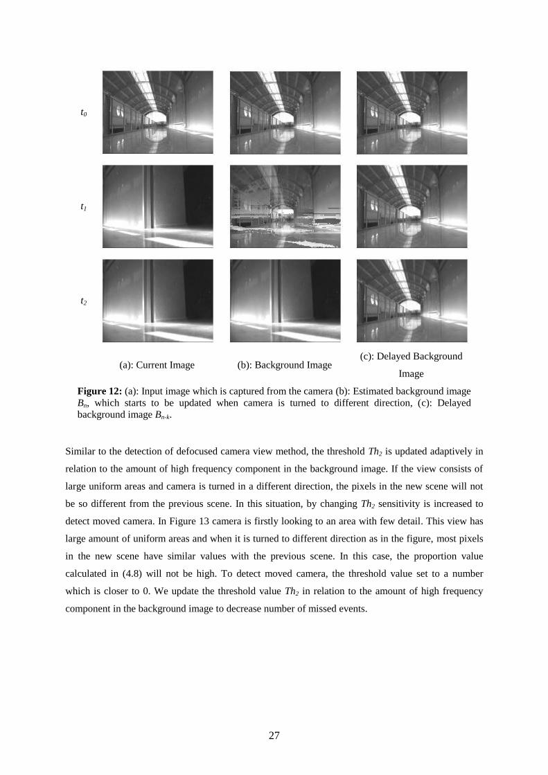
24. (a): captured image at time t0 when there are moving objects in the scene (b): captured
image at time t1 when there are moving objects in the scene ................................................. 41
25. (a): Background image at time t0 (b): Delayed background image at time t0 (c):
Background image at time t1 (b): Delayed background image at time t1 ............................... 43

xiii
26. (a): Background image which belongs to a non covered view at time t0 (b): Background
image of the covered view at time t1 (c): Entropy graphic..................................................... 45
27. (a): 2D red and green values of non covered view (b): 2D L1R histogram of non covered
view (c): 2D red and green values of covered view (d): 2D L1R histogram of covered view
............................................................................................................................................... 46
28. (a): Histogram of current image when camera view is covered (b): histogram of
background image when camera view is covered (c): histogram of difference image when
camera view is covered .......................................................................................................... 47

xiv
LIST OF ABBREVIATIONS
FFT : Fast Fourier Transform
ZNCC : Zero-Mean Normalized Cross Correlation
VSAM : Video Surveillance And Monitoring
1D : One Dimensional
2D : Two Dimensional
3D : Three Dimensional
OpenCV : Open Computer Vision Library
OS : Operating System

1
CHAPTER 1
INTRODUCTION
“At the front door, we unscrew light bulbs, adjust cameras, cover them with rubber gloves
if they do not move. Spray paint would be effective also at taking care of cameras that do not move.1”
Surveillance system operators often watch high number of cameras simultaneously and these systems
are left unattended at certain times which result in important events that require immediate actions to
be taken are missed such as deliberate attempts to tamper with a camera. In the recent years, computer
assisted algorithms which analyze the images from the cameras and warn the operator regarding such
events is found to be useful. In such systems, low number of false alarms is necessary. The high
number of false alarms results in alarms being ignored by the operator and renders the system
ineffective. Hence, such systems are expected to have low false alarm rate while having high true
alarm success rate. Also low computational complexity is required as high number of cameras needs to
be observed simultaneously or the algorithms are run on a camera or embedded system with limited
computational power.
On 17 May 2009, we read from the news reports, “Mexican authorities are conducting a massive
manhunt after more than 50 inmates were freed in one of the most daring prison escapes in the
country’s escalating drug wars. 2
”. A video was captured from a security camera when this escape
occurred. In this video, the prisoners cover the security camera with an object to prevent from being
seen which is seen in Figure 1. If there had been a system which warns the surveillance operator when
one of the security cameras is tampered, the escape may have been prevented.
Camera tampering which is also often referred to as camera sabotage in the literature, can be defined
as deliberate physical actions on a video surveillance camera which compromises the captured images.
1 Notes of a law enforcement officer to give readers some insight into the mind and methods of potential
attackers: http://www.survivalblog.com/2009/02/real_world_observations_on_fig.html 2 17 May 2009 news on http://www.independent.co.uk/news/world/americas/more-than-fifty-escape-in-mexican-
jailbreak-1686709.html

2
In this thesis we cover the following tampering types:
Defocused Camera View: Focus setting of a camera is changed and this results in reduced visibility.
Moved Camera: Turning a camera to make it point to a different direction.
Covered Camera View: Camera view is covered with a foreign object.
There are only a few methods in the literature which are aimed to detect the above sabotages. In this
thesis, new methods are proposed to detect the above sabotage types and these methods are compared
with the methods in [1-3]. In [1], wavelet based methods are proposed to detect defocused camera
view and covered camera view. However no method is proposed to detect camera displacement. The
algorithms proposed in paper [1] are based on a background model which is used as a base image
together with its wavelet transform. In [2], an edge background model is used to detect camera
tampering. However large objects or crowd of people moving in front of the camera could change the
image characteristics significantly and cause false alarms. In [3], the authors propose keeping a short
term and a long term pool of recent images. With each new image, these pools are updated and three
dissimilarity functions are calculated for all the images in these pools. This makes real-time operation
difficult due to the high number of computations required. Also this method doesn‟t identify the type
of tampering as any kind of dissimilarity between the short term pool and the long term pool is flagged
as tampering.
In this thesis we aim to detect camera tampering with robust methods which finds camera tampering
events in different environments and generates fewer number of false alarms. These algorithms use an
adaptive background image which is compared with the incoming frames from the video camera and
with a delayed background image. We also keep track of the moving areas of the image and use a
block based operation to reduce false alarms. This adaptive method is robust to moving objects in
front of the camera.
(a)
(b)
(c)
Figure 1: (a): Security camera view at time t0 where a person is preparing to cover the
camera view (b): Security camera view at time t1 where a person starts to cover the camera
view (c): Security camera view at time t2 where a person covers the camera view

3
Block diagram of the system is given in Figure 2. The system is composed of a video camera which is
located on a non-moving surface and a platform such as PC where the algorithms are run. The system
is based on the principle that when camera tampering occurs, the most recent frames captured by the
camera will be significantly different than the background image which stores older frame‟s
information. When a new frame is captured by the camera, firstly the background image is updated.
After updating the background image sabotage detection algorithms compare the background image to
the newly captured image to find whether a camera tampering has occurred. If no sabotage is detected,
the system works usual. However, if the system detects any kind of sabotage, an alarm is triggered to
warn the surveillance system operator.
This thesis is composed of six chapters. Chapter 1 introduces the camera tampering types, and the
approaches proposed in this thesis. In this chapter, we give introductory information about the system
proposed in this thesis. Because background subtraction technique is used by the other techniques in
the literature, we explain it before literature review in chapter 2. In this chapter, firstly the background
subtraction methods in the literature are given. After that the background subtraction method that we
use is explained and we discuss the rationale for choosing this particular technique. In chapter 3, the
methods in the literature are given. In chapter 4, the algorithms to detect different camera tampering
types are proposed. Detection of defocused camera view, detection of changed camera view and
detection of covered camera view algorithms are separately explained. Following these, in chapter 5
the experimental results are given. Performance of the methods in the literature is compared to the
methods which are proposed in this thesis and the results in various cases are discussed. In the last
section conclusions and future work are summarized.
Figure 2: Block Diagram of the Camera Tampering Detection System
4
CHAPTER 2
BACKGROUND SUBTRACTION
2.1 Overview Background subtraction is a widely used approach for segmenting out objects in the scene. We use this
technique to detect the stationary parts of the video. As camera tampering makes newly captured
frames significantly different than the older frames, we use estimated background images for camera
tamper detection by comparing them to newly captured frames. There are several methods for
performing background subtraction in the literature [4]. In this chapter we give information about
these techniques. After that the background subtraction method used in the thesis is explained.
2.2 Background Subtraction Methods in the Literature Background subtraction is used for segmenting out moving objects in a scene and finding the non
changing parts of a scene. There are several methods to perform background subtraction in the
literature. All these methods aim to estimate background view from a sequence of frames. These
methods face many challenges to make good estimation of background model [5]. Illumination change
is one of these challenges. Background subtraction methods must be robust against changes in
illumination to give good results. Other challenges are non-stationary objects such as swinging leaves,
rain, snow, shadow and speed of the background subtraction method.
In [4], the author examines different background subtraction methods according to their speed,
memory requirements and accuracy. These methods are:
Running Gaussian average
Temporal median filter
Mixture of Gaussians
Kernel density estimation (KDE)
5
Sequential KD approximation
Cooccurence of image variations
Eigenbackgrounds
Running Gaussian average: This method is a pixel based background subtraction method. In this
method, Gaussian probability density function is used for estimating background image‟s pixel values.
The background model at each pixel location is based on the pixel‟s recent history [4]. The method is
proposed in [6] and at each t frame, the It pixels value classified as non-stationary parts of the video if
the inequality below is satisfied:
𝐼𝑡 − 𝜇𝑡 > 𝑘𝜎𝑡 (2.1)
where k is a constant which can be used to change sensitivity. µt and σt are the two parameters of
Gaussian probability density function. These values are calculated as:
𝜇𝑡 = 𝛼𝐼𝑡 + 1 − 𝛼 𝜇𝑡−1
𝜎𝑡2 = 𝛼 𝐼𝑡 − 𝜇𝑡
2 + 1 − 𝛼 𝜎𝑡−12
(2.2)
where It is the current value of the pixel and µt-1 is the previous average value. α is update parameter
and used to change the stability of background model.
This method works fast and requires low memory. As the model is explained for intensity images like
in [6], its extensions can be made for color images [4].
Temporal median filter: In this method the previous N frames of video are buffered, and the
background is calculated as the median of buffered frames [7]. In his paper [4], Piccardi describes this
method as “The main disadvantage of a median-based approach is that its computation requires a
buffer with the recent pixel values. Moreover, the median filter does not accommodate for a rigorous
statistical description and does not provide a deviation measure for adapting the subtraction
threshold.”
Mixture of Gaussians: This method can handle multi model background distributions [5]. This
technique is proposed in [8] and it provides a description both background and foreground. In [8] the
probability of observing a certain pixel value, x, at time t is described by means of a mixture of K
Gaussian distributions:

6
𝑃 𝑥𝑡 = ωi,t ∗
𝐾
𝑖=1
𝛼𝐼𝑡 + η 𝑥𝑡 , 𝜇𝑖 ,𝑡 ,∑i,t
η 𝑥𝑡 , 𝜇 ,∑ = 1
2𝜋 𝑛/2 ∑ 1/2 𝑒−
12 𝑥𝑡−𝜇 𝑡
𝑇 ∑ −1 𝑥𝑡−𝜇 𝑡
(2.3)
where ωi,t is an estimate of weight of the ith
Gaussian in the mixture at time t, ∑i,t is the covariance
matrix of the ith
Gaussian in the mixture at time t, and where η is a Gaussian probability density
function.
In this method, to discriminate background distributions from foreground distributions other properties
of the distributions are used. In [4], it is given as “first, all the distributions are ranked based on the
ratio between their peak amplitude, ωi, and standard deviation,σi. The assumption is that the higher
and more compact the distribution, the more is likely to belong to the background. Then, the first B
distributions in ranking order satisfying:
𝜔𝑖 > 𝑇
𝐵
𝑖=1
(2.4)
with T an assigned threshold, are accepted as background.”
With this method, background subtraction can be done without keeping a large buffer of video frames.
The accuracy of this model is higher when multi valued background is needed. When the objects in the
background is not permanent like the scene consist of swinging leaves, rain, snow or sea waves, the
performance of this method is better than the other two methods explained above [4].
Kernel Density Estimation: With this method the background probability density function is given
by the histogram of the n most recent pixel values and each frame is smoothed with a Gaussian kernel
[4]. Elgammal et al. in [9] proposed non-parametric method and in this method the background
probability density function is given as sum of Gaussian kernels. The probability of observing a
certain pixel value, x, at time t is described as:
𝑃 𝑥𝑡 = 1
𝑛 η 𝑥𝑡 − 𝑥𝑖 ,∑t
𝑛
𝑖=1
(2.5)
where η is a Gaussian probability density function and ∑t is the covariance matrix at time t. If P(xt) is
greater than a threshold the pixel, x, is classified as background.
Kernel Density Estimation method is more complex that the background subtraction methods
explained so far [4]. This method requires high memory and works slow. However, the accuracy of

7
this method is high [9].
Sequential Kernel Density Approximation: Because mean-shift vector techniques which can be
used for background estimation has a very high computational cost, Sequential Kernel Density
Approximation technique proposed as an alternative [4]. In [10], Han et al. proposed a method which
uses the mean-shift vector for only an offline model initialization. They detect the initial set of
Gaussian modes of the background probability density function in the offline model initialization
process. In this method, heuristic procedures are used for adaptation, creation and merging the existing
modes to provide real time background model update.
In [10], Sequential Kernel Density Approximation method is compared to Kernel Density Estimation
method by using 500 frame test videos. They found that; Sequential Kernel Density Approximation
method is faster and requires lower memory than Kernel Density Estimation method.
Cooccurrence of image variations: In [11] Seki et al. propose a method which is based on the idea
that neighboring blocks of background model‟s pixels vary in a similar way over time. They define
stationary backgrounds impractical because the background scenes are not stable especially in the
outdoor scenes. According to their experience, the performance of stationary backgrounds are bad
when illumination changes and motions in background objects such as swinging leaves, rain or snow.
The proposed method in [11] aims to improve detection sensitivity by dynamically narrowing the
ranges of background image variations for each video frame. In this method block based processing is
done. This method is defined in two phases. In the first phase, a certain number of samples used to
compute first the average for all the blocks then the difference to find image variations. After that
covariance matrix and eigenvector transformation is computed. Aim of the first phase is to learn
background image pattern. In the second phase, image blocks are classified as background or
foreground. Eigen image variations of image blocks are used to classify these blocks as background or
foreground.
Cooccurance of image variations method is a complex and effective method. According to
experimental results in [4], this method is slower and requires more memory than all the other
methods explained. However, the accuracy of this method is reasonably high.
Eigenbackgrounds: Eigenbackground subtraction is a commonly used method for segmenting out
stationary parts of a video [12]. In this method newly coming frames are compared to background
model to find foreground of a video by using eigen-value decomposition.
In [4] this method is explained in two phases. The first phase is called learning phase and in this phase

8
a certain number of video frames are acquired and an average image is computed. After that the
covariance matrix is calculated and the best eigenvectors are stored in a matrix. In the second phase
which is called classification phase, foreground and background pixels are detected. When a new
frame is acquired from the video, it is projected onto the eigenspace. This projected image then
projected onto the image space. Finally, absolute values of the difference of these two projected
images‟ pixel values are compared to a threshold. If the value is greater than the threshold,
corresponding pixel is classified as foreground.
According the experiments in [4], the accuracy of this method better than the other methods explained
above. Its memory requirements are proportional to the number of recent images which are used to
calculate average image. The cost of the method about speed is associated with the number of best
eigenvectors stored in the matrix.
2.3 Background Subtraction Method of Video Surveillance And Monitoring
(VSAM) System Among various methods for subtraction of background in the literature, we based ours on the adaptive
background subtraction method of Video Surveillance And Monitoring (VSAM) System [13] as it
provides a simple, low computational cost alternative. Even though there are more sophisticated
background subtraction methods in the literature, we chose this method as the lower computational
cost is more important than accuracy for camera tampering detection applications.
Let In(x,y) represent the intensity value at pixel position (x,y) in the nth frame. Estimated background
image is represented as Bn+1 and value at the same pixel position, Bn+1(x,y) is calculated as follows:
𝐵𝑛+1 𝑥,𝑦 = 𝛼𝐵𝑛 𝑥,𝑦 + 1 − 𝛼 𝐼𝑛 𝑥,𝑦 𝑖𝑓 𝑥,𝑦 𝑖𝑠 𝑛𝑜𝑡 𝑚𝑜𝑣𝑖𝑛𝑔
𝐵𝑛 𝑥,𝑦 𝑖𝑓 𝑥,𝑦 𝑖𝑠 𝑚𝑜𝑣𝑖𝑛𝑔
(2.6)
where Bn(x,y) is the previous estimate of the background intensity value at pixel position (x,y) and α is
a positive real number where 0< α <1. α is selected close to 1 and B0(x,y) is set to the first image
frame I0(x,y). A pixel is said to be moving if the corresponding intensity values in In and In-1 satisfy the
following:
𝐼𝑛 𝑥,𝑦 − 𝐼𝑛−1 𝑥, 𝑦 > 𝑇𝑛 𝑥,𝑦 (2.7)
where Tn(x,y) is an adaptive threshold value for pixels positioned at (x,y). After each background
update, all the threshold values corresponding to each pixel position is also updated as follows:
𝑇𝑛+1(𝑥,𝑦) = 𝛼𝑇𝑛 𝑥,𝑦 + 1 − 𝛼 𝑐 𝐼𝑛 𝑥,𝑦 − 𝐵𝑛 𝑥,𝑦 𝑖𝑓 𝑥,𝑦 𝑖𝑠 𝑛𝑜𝑡 𝑚𝑜𝑣𝑖𝑛𝑔
𝑇𝑛 𝑥,𝑦 𝑖𝑓 𝑥,𝑦 𝑖𝑠 𝑚𝑜𝑣𝑖𝑛𝑔
(2.8)

9
where c is a real number greater than one. In this study we set initial values of all threshold values to
128 over 255. To increase the sensitivity the parameter c is reduced.
In this method, each pixel is compared to its corresponding adaptive threshold value to find whether
the pixel is moving or not. These adaptive threshold values are updated according to (2.8) after all
background estimation process. If a pixel is found as moving, its corresponding threshold value
doesn‟t change. If a pixel is marked as not moving, its related threshold value is changed in terms of
absolute value of the difference between current frame and background image‟s pixel values. Adaptive
threshold makes the pixels in the background image where there is a high activity more sensitive to the
changes in the current image.
Figure 3 shows the results of background subtraction for a scenario. In this figure, each row shows a
certain time and each column shows change in the images which are used in the background
subtraction method over time. Figure 3(a) shows the observed images, Figure 3(b) shows the
background model for the observed images, Figure 3(c) shows the adaptive threshold values according
to each pixel of the observed images and Figure 3(d) shows the foreground images.
In the first horizontal group of the figure two people are in the scene and they are moving at time t0.
As seen from the foreground image, these moving people are classified as foreground. Third image at
time t0, shows the adaptive threshold values and in this image the pixels that the two people are
passing are distinctive. The values of these pixels which can also be depicted as moving pixels are
greater than the other values in the adaptive threshold image. In our implementation of this
background subtraction method, initial values of adaptive threshold values are set to 128. The adaptive
threshold values of moving pixels are not changed according to (2.8) while the adaptive threshold
values which are not moving are changed. In this case because the differences between the non
moving pixels of In and Bn are not high, their corresponding adaptive threshold values are decreased.
As seen from the adaptive threshold image, the values of non moving pixels are less than the values of
moving pixels. In this background subtraction method, background model is slowly updated. When a
new object enters the scene, it takes a certain time to the object to become hardly visible in the
background. Similarly, when an existing object leaves the scene, it takes a certain time to the object to
be removed from the background. In the first horizontal group, some scarcely visible objects are seen
in the background image. The people who are passing through the scene are scarcely visible in the
background image. Because they are not stationary, they don‟t become hardly visible in the
background image. On the contrary, the scarcely visible objects in the background image will be
invisible after a short period of time.

10
In the second horizontal group of Figure 3 there are no moving objects in the scene at time t1. The
people who were passing through have left the scene. Because the input image consists of stationary
objects, the foreground image is seen as totally black. In the background image of this group the
scarcely visible objects which are seen in the previous background image become invisible. Adaptive
threshold image of this group is also different from the previous one. All the pixels of the input image
are classified as not moving and this causes the adaptive threshold values to change.
In the third horizontal group, the two people again enter the scene at time t2. In the foreground image,
the pixel values where the two people are standing are specified with white values. Because threshold
values are adapted over time, this time the pixels that the people are passing are not seen in the
t0
t1
t2
t3
(a) Current Image (b) Background
image (c) Adaptive
Threshold (d) Segmented
Foreground
Figure 3: Background Subtraction Method of VSAM system. In this figure, horizontal groups show
the relation between input, background, adaptive threshold and foreground. This scenario is running
from top to down.

11
background image. In the first horizontal group, the pixels can be seen scarcely visible in the
background image. Over time adaptive threshold values changed to enhance background estimation.
In the last horizontal group of Figure 3, the two people are seen in the scene and this causes the
corresponding pixel values to have white values in the foreground image at time t3. Background image
of this group consists of stationary parts of the video.
When an object enters or leaves the scene, it takes some time to the background model to become free
from moving objects. If the background subtraction method detects a new object in the scene which is
not exist in the previous scene, and the related pixels are not moving, the objects start to become a part
of background model. In a similar way, when an object leaves the scene and the related pixels are
classified as non-moving, the background model starts to be updated to make the object invisible. In
Figure 4 a new object enters the scene and the background model updates over time. In the end, the
object becomes hardly visible in the background image.
(a)
(b)
(c)
Figure 4: (a): Background image at time t0 (b): Background image at time t1 where a new
object has entered the scene (c): Background image at time t2 where the object is hardly visible

12
CHAPTER 3
LITERATURE REVIEW
3.1 Overview In this chapter we review the existing approaches for camera tamper detection in the literature. There
are methods to detect tampering of recorded images. For example, in [14] a watermarking technique is
proposed for tamper detection in digital images. This method divides images into blocks and by
comparing correlation values from different blocks of the images it enables us to distinguish malicious
changes. Another method proposed by Roberts in [15] and this method aims to authenticate images
captured by a security camera and localise tampered areas.While these methods bring new
contributions, they are not directly related to our problem. In this thesis we aim to create some
methods which monitors live video and detects defocused camera view, moved camera and covered
camera view.
There are many researches in computer vision which can be used to detect defocused camera view,
moved camera and covered camera view. However these methods are not directly concentrated on
camera tamper detection problem. In order to detect defocused camera view there are many researches
which may be employed. For example, Lim et al. in [16] proposed a method which aims to detect out-
of-focus photographs. They describe an algorithm that automatically determines if the captured
photograph is out-of-focus through image analysis. This method is specialized for digital photograph
machines and may not convenient in our case. This and similar methods are work on a single image. In
our case, there may be some transient conditions that single frame of a video may be out-of-focus not
implying camera tampering.
There are also many techniques which might be employed to detect covered camera view. For
13
example, in [17] a technique is proposed in order to detect gradual transitions in video sequences and
automatically identifying its type. This technique works fine when smooth transitions occur. However,
camera tampering is a rapid action that physically affects camera view. In [18] a method is proposed to
detect scene change which is also depicted as shot change. The technique is based on the tracking
boundary points in the edges, which is resistant to object motions and works well under gradual
transition. Because there are essential differences between camera tampering detection and shot
detection, this technique is not adequate for detecting covered camera view. Shot detection is used to
split up a video into basic temporal units which are called shots, while detection of covered camera
view is concerning of camera tampering.
In [19] a factorization method is proposed in order to estimate camera motion from stream of images.
It gives information about motion of the camera. In [20] another method is proposed to detect camera
motion. This approach minimizes both image error (i.e. noise) and the epipolar error (geometric
problem which occurs when projecting a 3D point onto the 2D images) to get optimal motion
estimation. Both of these methods are one of the studies in the camera motion estimation area.
However, these and similar techniques are not convenient for estimating camera motion where a
person moves it to point in a different direction. In our problem estimation of the motion of the camera
is not as important as simply recognizing that camera motion has occurred.
There are only a few methods in the literature which are directly aimed to detect camera tampering.
These methods all take a live video as input, and detect one or more sabotage types explained above.
In [1], wavelet based methods are proposed to detect defocused camera view and covered camera
view. However no method is proposed to detect camera movement. In [2], the methods for detecting
camera tampering are based on an edge based background model. This background model is not robust
against large objects or crowd of people moving in front of the camera and this result in false alarm
detection. In [3], short term and long term pools are used. When a new frame acquired from video,
these two pools are updated and three dissimilarity functions are calculated for all images in these
pools. Computational complexity of this method is very high and it doesn‟t identify the sabotage type
as defocused camera view, moved camera view and covered camera view. In [21], some methods are
proposed for surveillance systems inside a moving platform such as vehicle. Because our problem is
concerning the camera tampering where the camera is located on a steady place, the methods in this
research are not investigated in detail.
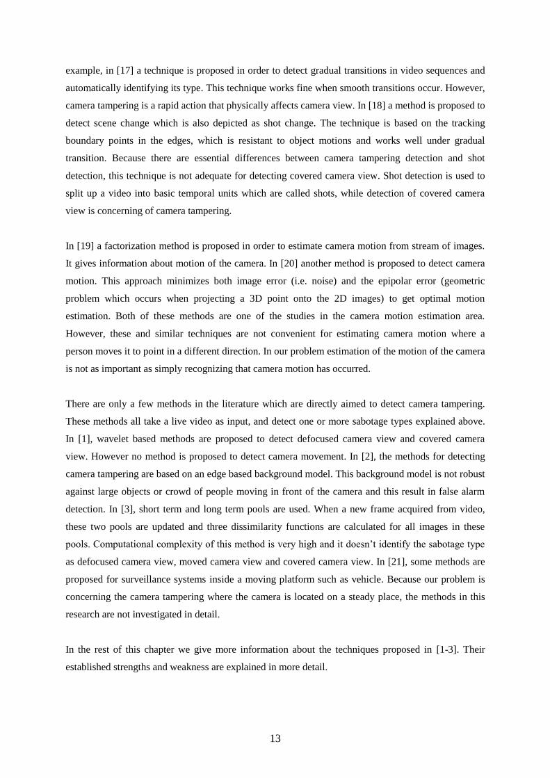
In the rest of this chapter we give more information about the techniques proposed in [1-3]. Their
established strengths and weakness are explained in more detail.

14
3.2 Camera Tamper Detection Using Wavelet Analysis for Video
Surveillance In this method, two algorithms are proposed to detect covered camera view and defocused camera
view [1]. These two algorithms are based on a background model which is proposed in [13]. The
background subtraction method is extended in this research to make it work in wavelet domain. The
authors estimate the background scene from the wavelet coefficients. Foreground objects and their
wavelet transform changes in time. The equations given in [13] which are used to estimate background
view and adaptive threshold values are modified as follows:
Wj𝐵𝑛+1 𝑘, 𝑙 = 𝛼Wj𝐵𝑛 𝑘, 𝑙 + 1 − 𝛼 Wj𝐼𝑛 𝑘, 𝑙 𝑖𝑓 WjIn 𝑥, 𝑦 𝑖𝑠 𝑛𝑜𝑡 𝑚𝑜𝑣𝑖𝑛𝑔
Wj𝐵𝑛 𝑘, 𝑙 𝑖𝑓 WjIn 𝑥,𝑦 𝑖𝑠 𝑚𝑜𝑣𝑖𝑛𝑔
(3.1)
Wj𝑇𝑛+1 𝑘, 𝑙 =
𝛼Wj𝑇𝑛 𝑘, 𝑙 + 1 − 𝛼 𝑐 Wj𝐼𝑛 𝑘, 𝑙 − Wj𝐵𝑛 𝑘, 𝑙
, 𝑖𝑓 WjIn 𝑥,𝑦 𝑖𝑠 𝑛𝑜𝑡 𝑚𝑜𝑣𝑖𝑛𝑔
Wj𝑇𝑛 𝑥,𝑦 , 𝑖𝑓 WjIn 𝑥,𝑦 𝑖𝑠 𝑚𝑜𝑣𝑖𝑛𝑔
(3.2)
where WjBn(k,l) shows the coefficient value of the wavelet image for pixel positioned at k,l.
To detect covered camera view, this method uses histogram values of the current frame and the
background frame. Maximum values of the histogram values are compared to check if the current
value has a higher peak than the background value. After that, histogram of absolute difference image
is checked to see the amount of values near the black end. These comparisons are done in low-low
wavelet band. This selection increases the robustness of the algorithm, because small changes are
discarded by the low-pass filter of wavelet transform.
When a camera view is defocused, small scale detail of the video disappears. In this method wavelet
low-high, high-low and high-high sub-bands are used for calculating the high frequency values of
current image and background image. Edges of the images are available in these sub-bands. High
frequency data of current image and background image is calculated in the following equations:
EHF 𝐼𝑛 = 𝑊𝐿𝐻𝐼𝑛
𝑘 ,𝑙
+ 𝑊𝐻𝐿𝐼𝑛
𝑘 ,𝑙
+ 𝑊𝐻𝐻𝐼𝑛
𝑘 ,𝑙
EHF 𝐵𝑛 = 𝑊𝐿𝐻𝐵𝑛
𝑘 ,𝑙
+ 𝑊𝐻𝐿𝐵𝑛
𝑘 ,𝑙
+ 𝑊𝐻𝐻𝐵𝑛
𝑘 ,𝑙
(3.3)
where WLHIn, WHLIn and WHHIn are the horizontal, vertical and diagonal sub-bands of single stage
wavelet transform of In respectively. High frequency value of current image and the background image
are compared with some tolerance to detect whether the camera view is defocused or not. If high
15
frequency value of current image is smaller than the high frequency value of background image, the
camera view detected as tampered.
In this camera tamper detection method there are some techniques which aim to reduce false alarm
detection rate. Persistency check is one of the measures against false alarms. This function checks if
the tampering cases occur in different consecutive time instants before triggering an alarm. Edge
correspondence check is another method for reducing false alarm rate. In this function camera view is
checked to confirm that camera still monitoring the same scene. If it is not, the results of covered
camera view and defocused camera view algorithms are discarded. Last measure is low light
conditions. If the level of light is less than a threshold, no calculation is done to find camera
tampering.
3.3 Automatic Control of Video Surveillance Camera Sabotage In this method [2], three algorithms are proposed to detect covered camera view, moved camera and
defocused camera view. These algorithms are based on an edge based background model. The main
concept is the comparison between the new frames with the older frames called the background model.
The background model which is used in this camera tamper detection technique includes only the
information at the edges of the stationary objects belonging to the background. The background image
contains information on the edges of the current image. To ensure that an edge belongs to the
background image, the following calculation is done for M consecutive frames.
𝐵𝑛 = 𝐷𝑖
𝑛+1 𝑀−1
𝑖=𝑛𝑀
(3.4)
where Di is the edge matrix computed for frame i. The pixels in Di take value 1 if it belongs to an edge
and 0 otherwise. To allow the system for slow changes of the background, the matrix B is computed
for each M new frames, and the background image is updated according to:
𝑃𝑛 = 𝛼𝑃𝑛−1 + 1 − 𝛼 𝐵𝑛 (3.5)
where α is a parameter between 0 and 1. If it is closer to 1 the background updates slowly. Only the
pixels which have been computed as edges for an enough number of times (the authors in [2] set it Pn
≥ M/2) are considered to belong to the background model.
The entropy of the pixels belonging to the background model is computed to detect whether the
camera view is covered or not. When camera view is covered partially or totally by an object, the
corresponding pixels in the background image turn to zero. In this situation, the entropy of the
background image decreases. Entropy is calculated as follows:

16
𝐸 = − 𝑃𝑘𝑘
𝑙𝑛 𝑃𝑘 (3.6)
where Pk is the probability of appearance of the gray level k in the image. Because ln(0) is equals to
infinity entropy calculation isn‟t done when Pk equals to zero. Depending on the background model
this calculation is done after each M consecutive frame arrives. In this method camera view is said to
be covered when the current entropy is smaller than a threshold. This method may be extended for
partially covered camera view cases. To enable the system to detect partially covered camera view, the
image is divided into blocks of equal size and entropy calculation is done for each block. In this
extended method, sabotage is detected when the current entropy for at least one of these blocks are
smaller than a threshold.
Defocused camera view results in degradation of the edges. In this camera tamper detection method,
the authors simply compare the number of edges in the background image and the current image.
When a camera view is defocused, the number of edges in current image will be significantly lower
than the number of edges in the background image.
In this research a block matching algorithm is used to detect whether camera view is moved or not.
Zero-Mean Normalized Cross Correlation (ZNCC) is calculated from the current frame and the
previous frame to match them. To speed up the calculations, only the pixels of the background model
are taken into account. This method tries to match the same edges of current frame and previous frame
and by this way it finds the amount of shift between two frames. If the shift is greater than a threshold,
camera view is said to be moved. Zero-Mean Normalized Cross Correlation is calculated as follows:
𝑍𝑁𝐶𝐶 = ∑ 𝐼𝑖−1 𝑥,𝑦 − 𝜇𝐼𝑖−1
𝑥 ,𝑦 𝐼𝑖 𝑥 + 𝑚,𝑦 + 𝑛 − 𝜇𝐼𝑖
𝜎𝐼𝑖−1𝜎𝐼𝑖 (3.7)
where Ii denotes current frame, Ii-1 denotes the previous frame, µ is the average value, σ is the standard
deviation, m is the horizontal axes and n is the vertical axes. The calculation is started from m and n
equals to zero and incremented up to the point where the ZNCC result is good enough. To speed up
algorithm ZNCC calculation isn‟t done if there is no edge on the (x,y) and (x+m,y+n) pixels of the
background image. If there is no displacement, the result of ZNCC equals to multiplication of width
and height of the image. If the result is smaller than a given threshold, it is interpreted as an error and
simply discarded. Displacements are tolerated up to 5 pixels. If it is greater than 5, an alarm is
triggered by this algorithm.
3.3 Real-Time Detection of Camera Tampering The method described in [3], is based on the principle that when camera tampering occurs, the most
recent frames of video will be significantly different than the older frames. In this method, the frames

17
which are acquired from video are stored in two different buffers. These buffers are called short term
pool and long term pool. Short term pool keeps newly coming frames and the size of this pool is 3-15
images depending on the setting chosen by the user. Long term pool keeps older frames and it stores
higher number of frames. When a frame is acquired from the video, it is stored in the short term pool.
If the number of frames in the short term pool is more than the allowed, the oldest frame is evicted
from the short term pool and inserted into the long term pool. Frames which are evicted from long
term pool are no longer stored. This structure may be thought as an alternative to the background
model in other camera tamper detection methods.
Each time a new frame is pushed into the short term pool, the short term pool and long term pool are
compared in order to determine if camera tampering has occurred. Every frame in short term pool is
compared to every frame in long term pool. Three dissimilarity functions are calculated for all these
comparisons. Medians of these three measurements are taken and compared to their corresponding
thresholds. The thresholds are tuned for optimal performance according to training videos. If any of
the thresholds are exceeded, the decision is made that camera tampering has occurred. However, this
method doesn‟t identify the type of tampering and as there are too many calculations in this approach,
it makes real-time operation difficult.
One of the image dissimilarity functions is histogram chromaticity difference. For each image a
normalized RGB histogram is calculated. In these histogram two axes shows the normalized red and
green components of each pixel. Blue component in this representation is uniquely determined by the
other two and ignored. The bin assignment for the 2D histogram is calculated as follows:
𝐵𝑖𝑛𝑅 = 𝑅𝑖𝑁𝑢𝑚𝐵𝑖𝑛𝑠𝑅/ 𝑅𝑖 + 𝐺𝑖 + 𝐵𝑖
𝐵𝑖𝑛𝐺 = 𝐺𝑖𝑁𝑢𝑚𝐵𝑖𝑛𝑠𝐺/ 𝑅𝑖 + 𝐺𝑖 + 𝐵𝑖 (3.8)
where Ri, Gi and Bi are the red, green and blue components of pixel i. The value of BinR and BinG in
the 2D histogram is incremented after this calculation. For example, the 2D histogram consists of 64
bins and the results for BinR and BinG are calculated as the following:
BinR = 25
BinG = 78
The value of bin expressed in Figure 5 incremented by one. In this figure 8x8 bins exist and the results
of BinR and BinG are normalized according to the number of bins.

18
To calculate histogram chromaticity difference, the sum of absolute value differences of the two
histograms is computed. This difference is given as:
𝐷𝑖𝑓𝑓𝑒𝑟𝑒𝑛𝑐𝑒1,2 = 𝐻1 𝑖, 𝑗 − 𝐻2 𝑖, 𝑗
𝑖 ,𝑗
(3.9)
When a new frame pushed into the short term pool, the difference is calculated for all the frames in the
short term and long term pools. After that the median value is taken and compared to a threshold
value. If it exceeds the threshold value, the condition is evaluated as true which means that camera
tampering has occurred.
Histogram L1R difference is another dissimilarity function which is used to detect camera tampering.
In this function, a 2D histogram is used again. However the axes of this 2D histogram are different
than the previous one. The axes of this histogram are the L1-norm and range of the red, green and blue
components of the pixel. The bin assignments are calculated as follows:
𝐵𝑖𝑛𝐿1 = 𝑅𝑖 + 𝐺𝑖 + 𝐵𝑖 𝑁𝑢𝑚𝐵𝑖𝑛𝑠𝐿1/3
𝐵𝑖𝑛𝐺 = max 𝑅𝑖 ,𝐺𝑖 ,𝐵𝑖 − min 𝑅𝑖 ,𝐺𝑖 ,𝐵𝑖 𝑁𝑢𝑚𝐵𝑖𝑛𝑠𝑅 (3.10)
where R is the range and L1 is the L1-norm. In this 2D histogram total number of bins may be
different than the previous one. L1-norm value of a pixel is proportional to its intensity and the range
is proportional to its saturation. The dissimilarity between two images is calculated again by summing
the absolute values of differences between the two histograms. Similarly, this measurement is done
when a new frame is pushed into the short term pool. Median value is compared to a threshold and if it
is greater than a threshold, camera view is said to be tampered.
Figure 5: 2D Histogram Bin Assignment
19
The last dissimilarity function proposed in this method is histogram gradient direction difference. In
this function each image is firstly convolved with the 3x3 Sobel kernels. After that, these images are
used to estimate gradient direction. In this dissimilarity function 1D histogram is used. The bin
assignments in this 1D histogram are done in a similar way. The bin assignment for pixel (i,j) is
calculated as:
𝐵𝑖𝑛𝐺𝑟𝑎𝑑𝐷𝑖𝑟 = 1/𝜋 𝐷𝑖𝑟 𝑖, 𝑗 + 𝜋/2 𝑁𝑢𝑚𝐵𝑖𝑛𝑠𝐺𝑟𝑎𝑑𝐷𝑖𝑟 (3.11)
where Diri,j is the gradient direction at pixel location (i,j). Gradient direction is thought as in the range
[-π, π]. Sum of absolute values of differences between two histograms are used as dissimilarity. Each
frame in short term pool and long term pool is compared with this image dissimilarity. The median
values are compared to a threshold to find whether the camera view is tampered or not.

20
CHAPTER 4
ADAPTIVE CAMERA TAMPER DETECTION ALGORITHMS
4.1 Overview In this chapter, we will explain the proposed algorithms which are used to detect defocused camera
view, moved camera and covered camera view. Firstly, we explain the detection of defocused camera
view method. In this method we use high frequency data of current and background frames to find
whether the camera view is defocused or not. After that we investigate the cases where the amount of
high frequency changes significantly. For these cases an extension of this method is proposed. In this
extended method, regularly changing parts of the images are ignored to reduce false alarm rate.
Secondly, we explain the detection of moved camera method. In this method, we use a delayed
background image and this image is compared with the background image to find if the camera is
moved to point in a different direction. Lastly, we give information about the detection of covered
camera view method. In the first step of this method histograms of the current and background images
are compared to detect whether camera view is covered or not. In the second step, histogram of
absolute difference image |In-Bn| is checked to see if most of the values are located near the black end.
4.2 Detection of Defocused Camera View Defocusing the lens of a camera or reduced visibility due to atmospheric conditions such as fog results
in degradation of edges in the captured image. In such a case, the high frequency data of the current
image In will be lower than the high frequency data of the background image Bn. In the proposed
algorithm, high frequency data in In and Bn are compared using Fast Fourier Transform (FFT). In
Figure 6 two frames of a video and their corresponding magnitude images which are obtained after
taking FFT are given. In the magnitude images, high frequency values are around the origin. In the
first horizontal group, camera view isn„t defocused and the image has strong edges resulting in high
frequency data in the magnitude image. In the second horizontal group, camera view is defocused
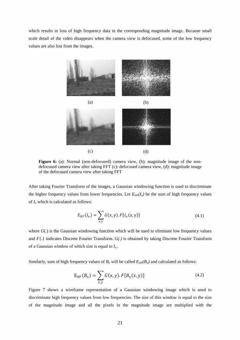
21
which results in loss of high frequency data in the corresponding magnitude image. Because small
scale detail of the video disappears when the camera view is defocused, some of the low frequency
values are also lost from the images.
After taking Fourier Transform of the images, a Gaussian windowing function is used to discriminate
the higher frequency values from lower frequencies. Let EHF(In) be the sum of high frequency values
of In which is calculated as follows:
𝐸𝐻𝐹 𝐼𝑛 = 𝐺 𝑥,𝑦 .𝐹 𝐼𝑛 𝑥,𝑦
𝑥 ,𝑦
(4.1)
where G(.) is the Gaussian windowing function which will be used to eliminate low frequency values
and F{.} indicates Discrete Fourier Transform. G(.) is obtained by taking Discrete Fourier Transform
of a Gaussian window of which size is equal to In..
Similarly, sum of high frequency values of Bn will be called EHF(Bn) and calculated as follows:
EHF 𝐵𝑛 = 𝐺 𝑥, 𝑦 .𝐹 𝐵𝑛 𝑥,𝑦
𝑥 ,𝑦
(4.2)
Figure 7 shows a wireframe representation of a Gaussian windowing image which is used to
discriminate high frequency values from low frequencies. The size of this window is equal to the size
of the magnitude image and all the pixels in the magnitude image are multiplied with the
(a)
(b)
(c)
(d)
Figure 6: (a): Normal (non-defocused) camera view, (b): magnitude image of the non-
defocused camera view after taking FFT (c): defocused camera view, (d): magnitude image
of the defocused camera view after taking FFT
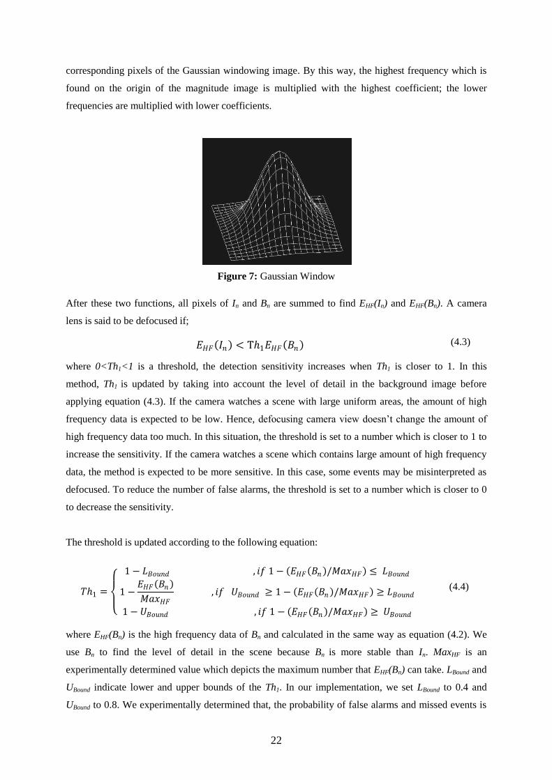
22
corresponding pixels of the Gaussian windowing image. By this way, the highest frequency which is
found on the origin of the magnitude image is multiplied with the highest coefficient; the lower
frequencies are multiplied with lower coefficients.
After these two functions, all pixels of In and Bn are summed to find EHF(In) and EHF(Bn). A camera
lens is said to be defocused if;
𝐸𝐻𝐹 𝐼𝑛 < T1𝐸𝐻𝐹 𝐵𝑛 (4.3)
where 0<Th1<1 is a threshold, the detection sensitivity increases when Th1 is closer to 1. In this
method, Th1 is updated by taking into account the level of detail in the background image before
applying equation (4.3). If the camera watches a scene with large uniform areas, the amount of high
frequency data is expected to be low. Hence, defocusing camera view doesn‟t change the amount of
high frequency data too much. In this situation, the threshold is set to a number which is closer to 1 to
increase the sensitivity. If the camera watches a scene which contains large amount of high frequency
data, the method is expected to be more sensitive. In this case, some events may be misinterpreted as
defocused. To reduce the number of false alarms, the threshold is set to a number which is closer to 0
to decrease the sensitivity.
The threshold is updated according to the following equation:
𝑇1 =
1 − 𝐿𝐵𝑜𝑢𝑛𝑑 , 𝑖𝑓 1 − 𝐸𝐻𝐹 𝐵𝑛 /𝑀𝑎𝑥𝐻𝐹 ≤ 𝐿𝐵𝑜𝑢𝑛𝑑
1 −𝐸𝐻𝐹 𝐵𝑛
𝑀𝑎𝑥𝐻𝐹 , 𝑖𝑓 𝑈𝐵𝑜𝑢𝑛𝑑 ≥ 1 − 𝐸𝐻𝐹 𝐵𝑛 /𝑀𝑎𝑥𝐻𝐹 ≥ 𝐿𝐵𝑜𝑢𝑛𝑑
1 − 𝑈𝐵𝑜𝑢𝑛𝑑 , 𝑖𝑓 1 − 𝐸𝐻𝐹 𝐵𝑛 /𝑀𝑎𝑥𝐻𝐹 ≥ 𝑈𝐵𝑜𝑢𝑛𝑑
(4.4)
where EHF(Bn) is the high frequency data of Bn and calculated in the same way as equation (4.2). We
use Bn to find the level of detail in the scene because Bn is more stable than In. MaxHF is an
experimentally determined value which depicts the maximum number that EHF(Bn) can take. LBound and
UBound indicate lower and upper bounds of the Th1. In our implementation, we set LBound to 0.4 and
UBound to 0.8. We experimentally determined that, the probability of false alarms and missed events is
Figure 7: Gaussian Window

23
higher when the threshold is smaller than LBound and greater than UBound. Because of that, we don‟t
allow the threshold to exceed these bounds.
In Figure 8, two images and their magnitudes are given. In Figure 8 (a) camera watches a scene which
contains less high frequency data and in Figure 8 (c), the same scene seen as defocused. As seen from
the magnitude images, the amount of high frequency data in defocused and non-defocused images are
not so different. In this case, we reduced the number of missed events by updating the threshold. The
magnitude images shown in this figure are filtered with a Gaussian windowing function.
In Figure 9, two camera views which are captured from the same scene and their magnitudes are
given. In Figure 9 (a), the amount of high frequency data is high. If this view is defocused as seen in
Figure 9 (c), the change of high frequency data in the magnitude image will be reasonably high. In this
situation, we reduced the number of missed events by setting the threshold to a number which is closer
to 0. The magnitude images shown in this figure are filtered with a Gaussian windowing function.
(a)
(b)
(c)
(d)
Figure 8: (a): non-defocused camera view with large uniform areas, (b): magnitude image of the
image (a) filtered with a Gaussian window (c): defocused camera view with large uniform areas,
(d): filtered magnitude image of the (c) filtered with a Gaussian window

24
Even though this method is useful for detecting the reduced visibility, there are cases in typical
surveillance scenarios where the amount of high frequency changes significantly which could
potentially generate false alarms. When new objects enter to the scene or objects leave the scene, total
amount of edges and hence the high frequency content in In changes. To handle such cases, the
algorithm is modified to ignore regularly changing parts of the images. Changing pixels are found and
marked using equation (4.5) and they are kept in moving state until they are observed to be non-
moving for a while.
𝑀𝑛(𝑥,𝑦) =
𝑀𝑛(𝑥,𝑦) + 𝛽 𝐼𝑛 𝑥,𝑦 − 𝐵𝑛 𝑥,𝑦
, 𝑖𝑓 𝑥,𝑦 𝑖𝑠 𝑚𝑜𝑣𝑖𝑛𝑔
𝑀𝑛(𝑥, 𝑦) − 𝛾 𝐼𝑛 𝑥,𝑦 − 𝐵𝑛 𝑥,𝑦 + 1
, 𝑖𝑓 𝑥,𝑦 𝑖𝑠 𝑛𝑜𝑛 𝑚𝑜𝑣𝑖𝑛𝑔
(4.5)
In this equation, Mn is the image which keeps track of the changing pixels related to nth frame. Initial
values of its pixels are set to 0. β and γ are constants and β is selected to be greater than γ to make a
pixel gracefully non-moving when no motion is observed.
Figure 10 shows the change of high frequency values when new objects enter or leave the scene.
(a)
(b)
(c)
(d)
Figure 9: (a): non-defocused camera view with large high frequency data, (b): magnitude
image of the image (a) filtered with a Gaussian window (c): defocused camera view with large
high frequency data, (d): filtered magnitude image of the (c) filtered with a Gaussian window

25
After finding the changing pixels, In and Bn divided into 8x8 pixel blocks. Each block is checked for
moving pixels, if the block contains any moving pixels, the pixels in this block are excluded from the
equation calculating the high frequency content in both In and Bn. Figure 11 shows an example of
exclusion of moving areas.
Amount of high frequency data in In and Bn are calculated using the following equations which
excludes the moving blocks. A block is said to be moving if Mn(x,y) ≠ 0 for any pixel in the block:
𝐸𝐻𝐹 𝐼𝑛 = 𝐺 𝑥,𝑦 .𝐹 𝐼𝑛 𝑥,𝑦
𝑥 ,𝑦
𝑘
𝑖=0
(4.6)
(a)
(b) Figure 11: (a): Image showing changing pixels, Mn where changing pixels are shown
white (b): Corresponding image which shows the ignored blocks. Black rectangles
show the ignored areas.
(a)
(b)
(c)
(d)
Figure 10: (a): An image which contains more high frequency component, (b): Magnitude of
the image (a) after FFT, (c): An image which contains less high frequency values, (d):
Magnitude of the image (b) after taking FFT.
26
𝐸𝐻𝐹 𝐵𝑛 = 𝐺 𝑥,𝑦 .𝐹 𝐵𝑛 𝑥,𝑦
𝑥 ,𝑦
𝑘
𝑖=0
(4.7)
where k is the number of blocks not having any moving pixels. Once EHF(In) and EHF(Bn) are found,
they are compared using the equation (4.3). Th1 is updated in the same way to equation (4.4). The
EHF(Bn) which is used to update Th1 is calculated without block based processing.
4.3 Detection of Moved Camera Turning a camera to make it point in a different direction is also a type of tampering. When a camera
is moved to a different direction, the background image Bn starts to be updated to reflect the changed
view. In the proposed algorithm we use another image which holds a delayed background image and
represented as Bn-k where k ϵ Z+. Bn-k is compared with Bn to find if a camera is moved to point towards
a different direction. A proportion value denoted with P is calculated by comparing each pixel on Bn to
corresponding pixel on Bn-k.
𝑃 = 𝑃 + 1 , 𝑖𝑓 𝐵𝑛 𝑥,𝑦 ≠ 𝐵𝑛−𝑘(𝑥,𝑦)
𝑃 , 𝑖𝑓 𝐵𝑛 𝑥, 𝑦 = 𝐵𝑛−𝑘 𝑥,𝑦
(4.8)
Camera is said to be moved to different direction if P>Th2K where 0<Th2<1 is threshold value which
increases sensitivity when it is closer to 0 and K is the total number of pixels.
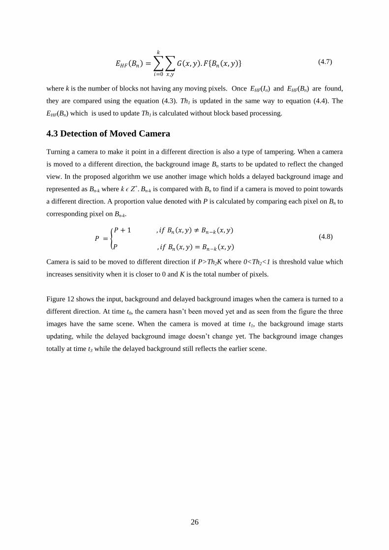
Figure 12 shows the input, background and delayed background images when the camera is turned to a
different direction. At time t0, the camera hasn‟t been moved yet and as seen from the figure the three
images have the same scene. When the camera is moved at time t1, the background image starts
updating, while the delayed background image doesn‟t change yet. The background image changes
totally at time t3 while the delayed background still reflects the earlier scene.
27
Similar to the detection of defocused camera view method, the threshold Th2 is updated adaptively in
relation to the amount of high frequency component in the background image. If the view consists of
large uniform areas and camera is turned in a different direction, the pixels in the new scene will not
be so different from the previous scene. In this situation, by changing Th2 sensitivity is increased to
detect moved camera. In Figure 13 camera is firstly looking to an area with few detail. This view has
large amount of uniform areas and when it is turned to different direction as in the figure, most pixels
in the new scene have similar values with the previous scene. In this case, the proportion value
calculated in (4.8) will not be high. To detect moved camera, the threshold value set to a number
which is closer to 0. We update the threshold value Th2 in relation to the amount of high frequency
component in the background image to decrease number of missed events.
t0
t1
t2
(a): Current Image (b): Background Image (c): Delayed Background
Image
Figure 12: (a): Input image which is captured from the camera (b): Estimated background image
Bn, which starts to be updated when camera is turned to different direction, (c): Delayed
background image Bn-k.

28
4.4 Detection of Covered Camera View When a camera view is covered with an object, histogram of In is expected to have higher values in a
specific range in the histogram compared to the Bn. Because most of the scene is occupied by the
covering object, a significant part of In is expected to have the color of the covering object or become
darker. In Figure 14, current and background images and their corresponding 32-bin histograms are
given when camera is covered by hand.
In [1], an algorithm which is used to detect covered camera view is proposed. The algorithm calculates
the histograms of In and Bn. In this algorithm there are two steps. If both of the steps are satisfied,
camera view is said to be covered. In this study we modified the first step of this algorithm. Let
max(H(A)) represent the bin number of which value is the maximum value in histogram of image A. In
(a) (b)
(c) (d)
Figure 14: (a): In when camera covered (b): Histogram of the image In when camera covered (c): Bn
when camera covered (d): Histogram of the image Bn when camera covered
(a) (b)
Figure 13: (a): Camera view where there are large uniform areas (b): Turned view of (a)
where most of the pixels have the similar values with the previous scene

29
the first step the values of maximum bin number and its neighbors of the histogram of In and Bn found
and compared to check if In has a higher peak than Bn. In the second step, histogram of the absolute
difference |In-Bn| is checked to see if most of the values accumulate near the black end.
32-bin histogram of an image will be called Hi(.) where 1≤i≤32. Both (4.9) and (4.10) are checked to
find whether a camera view is covered or not.
𝐻𝑚𝑎𝑥 𝐻 𝐼𝑛 − 1 𝐼𝑛 + 𝐻𝑚𝑎𝑥 𝐻 𝐼𝑛 𝐼𝑛 + 𝐻𝑚𝑎𝑥 𝐻 𝐼𝑛 +1 𝐼𝑛
> 𝑇3 𝐻𝑚𝑎𝑥 𝐻 𝐼𝑛 − 1 𝐵𝑛 + 𝐻𝑚𝑎𝑥 𝐻 𝐼𝑛 𝐵𝑛 + 𝐻𝑚𝑎𝑥 𝐻 𝐼𝑛 +1 𝐵𝑛
(4.9)
Th3 > 1 is threshold which can be increased for higher sensitivity of the algorithm. In the above
equation, if a bin value is smaller than 1 or greater than 32 their corresponding value is thought as 1 or
32 respectively. As seen from Figure 15, when camera view is covered the value which is obtained by
summing maximum bin number and its neighbors is greater in the histogram of In than in the
histogram of Bn. The related bins in the histogram of In and Bn are represented in Figure 15.
In the second step of the algorithm difference image is used. When camera view is not covered, the
difference image consists of totally black pixels. In this case, all the values of the difference image‟s
histogram are found in the first bin. If the camera covered with an object, In and Bn will be different
from each other and the values in the difference image‟s histogram will expand over the histogram.
Figure 16 shows the change in the histogram of difference image when camera view is covered. The
second step of the algorithm is given below:
Figure 15: Maximum bin number and its neighbors of the histogram of In and Bn when
camera view is covered

30
𝐻𝑖 𝐼𝑛 − 𝐵𝑛 > 𝑇4 𝐻𝑖 𝐼𝑛 − 𝐵𝑛
𝑘
𝑖=1
32
𝑖=1
(4.10)
Th4 > 1 is threshold which can be increased for higher sensitivity of the algorithm. Where 0 ≤ k < 32
and when it closer to the lower bound, sensitivity will be higher, typically k=3 is found to be
generating satisfactory results.

31
(a)
(b)
(c)
(d)
(e)
(f)
(g)
(h)
Figure 16: (a): In when camera view is not covered (b): Bn when camera view is not covered
(c): | In - Bn | when camera view is not covered (d): Histogram of | In - Bn | when camera view is not
covered (e): In when camera view is covered (f): Bn when camera view is covered (c): | In - Bn | when
camera view is covered (d): Histogram of | In - Bn | when camera view is covered

32
CHAPTER 5
EXPERIMENTAL RESULTS AND COMPARISONS
5.1 Overview We have tested the proposed algorithms in indoor and outdoor environments including real life
scenarios. The proposed methods in this thesis are compared to the methods in [1-3] and the strengths
and weakness of all these methods are experimentally illustrated in different test cases. In this chapter
we give detailed information about the testing environment, test data, testing scenarios and results.
5.2 Testing Environment
To test the proposed methods and compare with the methods in the literature, we captured a range of
images to reflect real-life camera tampering scenarios. Also to test the false alarms, we used some
video sequences from the i-LIDS dataset [22] which contain typical surveillance scenarios without any
camera tampering.
Each method explained in [2-3] is firstly implemented and tested with the same set of test videos. For
[1] there is already an existing implementation and the same scenarios have been tested with this
implementation. In [3], the authors propose a method which has high computational complexity. The
structure used in this method is given in Figure 17. When a new image captured from the camera, it is
inserted in the short term pool and the three dissimilarity measures are calculated. Assuming that,
there are m images in the short term pool and n images in the long term pool. When a new image
inserted in the short term pool, because each image in short term pool are compared to the images in
the long term pool according to three different dissimilarity measures, (m x n x 3) number of
calculations are required. We reduced the number of calculations by keeping the dissimilarity
measures in memory and only calculating the dissimilarities for images entering the two buffers.

33
When a new image is inserted into the short term pool, the oldest image in the short term pool is
evicted from this pool and inserted in to the long term pool. Hence, there exist 2 new images in the
pools. For the new image in the short term pool, n number of calculations is required and for the new
frame in the long term pool, m number of calculations is required. These calculations are done
according to the three dissimilarity functions which makes the total number of calculations 3 x (m + n)
when a new image inserted into the short term pool.
The algorithms have been implemented using C++ language and OpenCV library [23-24]. OpenCV is
a computer vision library originally developed by Intel. OpenCV has greater than 500 algorithms,
documentation and sample code for real time computer vision. This library is written in C, which
makes it portable to some specific platforms. The platforms where OpenCV can run are; Microsoft
Windows, Apple Mac OS X, Linux, Sony PSP3, VCRT
4 and other embedded devices [24].
In our implementations, we needed to set some parameters regarding speed and accuracy. Because
some parameters are not specified in [2, 3], we had to make some assumptions in their
implementations. To speed up the algorithms, the size of the images which are captured from the
camera is set to 160 x 120. Also we don‟t check camera tampering for all the frames. The algorithms
are run once for every 20 frames. This image size and frame rate is found to be sufficient for detecting
camera tampering.
3 Play Station Portable which is a handheld game console made by Sony
4 Real-Time OS on Smart camera: www.vision-components.com
Figure 17: Incoming images are stored in the short term and long term pools

34
5.3 Experimental Results In this part, we present the test results. Tampering types which are explained in above sections are
separately tested. The algorithms have been tested with the same test cases. Some images which are
taken from the test scenarios are shown here to explain these cases in more detail.
5.3.1 Defocused Camera View
The algorithms were tested on a total of 27 videos having 40 defocusing events. The videos were
captured in different environments and they contain a variety of test scenarios. Some of the videos are
used to test false alarm cases and they don‟t contain any defocusing event. The algorithms are forced
with the specific videos which are captured for exposing the vulnerabilities of the algorithms. Table 1
shows the results of defocused camera view tests.
Table 1: Defocused Camera Test Results for Different Algorithms
Algorithms Number of false
alarms
Number of
missed events
Percentage of
missed events
Aksay et al. [1] 5 7 17,5%
Gil-Jiménez et al. [2] 3 13 32,5%
Ribnick et al. [3] 4 14 35%
Proposed Method
(not ignoring moving
blocks)
27 6 15%
Proposed Method
(ignoring moving
blocks)
2 6 15%
As seen from the results, [3] gives the highest number of missed events. When we evaluated the test
videos in detail we observed that if the scene contains more red and green objects the sensitivity of this
algorithm increases. Since it uses red and green values to construct a 2-dimensional histogram and this
histogram is used for image dissimilarity measurement, red and green objects in the scene affect the
results positively. In Figure 18, 4 different red and green values 2D histogram are showed. The two
images which are in the first horizontal group of the figure belong to a scene where there are small
amount of red and green values. Figure 18 (a) corresponds to the non tampering case of the scene
where there is lack of red and green values. If the scene is defocused, the 2D histogram doesn‟t change
significantly as seen from the Figure 18 (b). However, if the scene contains large amount of red and
green values, defocusing lens of the camera will change the 2D histogram remarkably. Figure 18 (c)

35
belongs to a scene which has red and green objects. When its corresponding scene defocused, the 2D
histogram will change as seen in Figure 18 (d). As you see from these histograms, the change in this
scene is much more than the first scene.
When camera view is defocused, results of other dissimilarity functions used in [3] do not differ
sufficiently enough to detect this type of tampering. Even though the number of false alarms detected
by this method is not high, moving red or green objects potentially cause false alarms. When red or
green objects enter or leave the scene, the result of the 2D histogram changes significantly. This
significant change in the 2D histogram might result in false alarm detection.
(a)
(b)
(c)
(d)
Figure 18: (a): 2D red-green values histogram of a non defocused scene which contains less amount
of red and green values (b): 2D red-green values histogram of a defocused scene which contains less
amount of red and green values (c): 2D red-green values histogram of a non defocused scene which
contains large amount of red and green values (d): 2D red-green values histogram of a defocused
scene which contains large amount of red and green values

36
The method in [3] compares all the images in short term and long term pools which are explained in
chapter 3, when a new image captured from the camera. The medians of all these comparisons are
checked to see if they exceed a certain threshold. When a camera view is defocused, it takes some time
for it to affect the median of the comparisons. Therefore, this method detects tampering with some
delay -in the order of a few seconds-, after the event occurred. Another important thing to mention is
the fixed thresholds in this method. The authors mention that the thresholds are tuned for optimal
performance based on a set of training videos. However, there is no optimal threshold for all the cases
and the threshold needs to be modified for different scenes. For this type of tampering, thresholds may
be adaptive according to the amount of red and green values in the scene.
In [1], WLH, WHL, and WHH sub bands in wavelet domain are used to detect defocused camera view.
These sub bands represent the horizontal, vertical and diagonal details of the image respectively. As
seen from the test results, this method interprets some non tampering events as defocused camera
view. In this method, moving objects bring some detail to the sub bands used to identify defocused
camera view. Also, moving objects, when they move out of the scene, remove some detail from these
sub bands. This is interpreted as reduction in high frequency content and results in false alarms. All
the false alarms related to this method are observed to be due to the moving objects.
In [2], an edge based background model is used and to detect defocused camera view the edges in this
background model is compared to the edges in the current image. Defocusing the lens of a camera
causes degradation of edges in the current image and in this situation the number of edges in the
background image will be higher than the number of edges in the current image. However, in real life
there are moving objects in front of the camera and they change the number of edges in the current
image. Even if the camera is not defocused, the number of edges in the current image may be less than
the number of edges in the background image when some objects leave the scene. Some test cases
have demonstrated this weakness of this method. For example, in Figure 19, a person is studying at a
desk at time t0. At that time, the current edge image and the background edge image has nearly the
same number of edges. At time t1, the person leaves the desk and as seen from the images, the number
of edges in the current image is decreased. In this case, the method incorrectly identifies a defocused
camera view tampering.

37
Background image is updated to ensure that the edges of moving objects are not included in the
background image [2]. There are some cases that the stationary pixels which are positioned behind the
moving objects are not seen in the background image. In such cases, tampering events may be missed
because the number of edges is less than the current image. For example, a scenario is given in Figure
20 from the test cases. In this case a person is walking in front of the bookshelf. As seen from Figure
20 (b) the edges of the bookshelf and the person are seen in the current edge image. However edges of
the person and some edges of the bookshelf are not seen in Figure 20 (c) which represents the
background edge image. In this method, the edges of the background image are taken from non
moving objects and the objects which are seen on a certain number of consecutive frames. Because the
person is moving and preventing some edges of the bookshelf to be seen, background image has fewer
edges. If the camera is defocused in this situation, this method cannot detect the sabotage.
Our first method which doesn‟t ignore the moving parts on the images gives a high number of false
(a)
(b)
(c)
Figure 20: (a): Current image (b): Current edge image (c): Background edge image
(a)
(b)
(c)
(d)
Figure 19: (a): Current edge image at time t0 (b): Background edge image at time t0 (c): Current
edge image at time t1 (d): Background edge image at time t1

38
alarms. Because moving objects on the scene changes the high frequency content in the current image,
false alarms may arise. In this method high frequency content of the current and the background image
is compared to detect defocused camera view. When an object enters the scene, because of its edges, it
brings high frequency data to the current image. Similarly, an object leaving the scene, it causes
reduction in the high frequency data in the current image. In Figure 21, a car is seen in both current
and background image at time t0. The edges of the car correspond to high frequency data in frequency
domain. When the car leaves at time t1, the high frequency data of the car disappears from the current
image. Because the total amount of high frequency data decreases in the current image at time t1, a
false alarm is triggered by this method.
Ignoring the moving blocks reduces the false alarm rate while not affecting the true alarm rate. In this
method, only the blocks which don‟t contain any moving object are used to calculate the high
frequency data of the current and the background image. If we examine the same test case as in the
previous method, the blocks where the car passes through will be ignored. FFT operation is done for
other blocks of the current and background image and a Gaussian windowing function is applied to
each of these blocks to discriminate high frequency data. In current and background image high
frequency data of the blocks which are not ignored are summed to calculate total high frequency data.
After that the total high frequency values are compared to check whether the camera view is
defocused. Figure 22 shows the ignored blocks when the car in the previous example moves. Figure 22
(c) shows the 8x8 pixel blocks which contain moving objects and hence, will be ignored by this
method. In this image, the ignored blocks are shown with black rectangles.
(a)
(b)
(c)
(d)
Figure 21: (a): Current image at time t0 (b): magnitude image of current image after filtering
with a Gaussian window at time t0 (c): current image at time t1 (d): magnitude image of current
image after filtering with a Gaussian window at time t1

39
In this method, sometimes the defocused regions in the images are misinterpreted as moving and
hence taken out of consideration. This has caused missed events in the test cases. Generally, not all the
defocused blocks are interpreted as moving and the non ignoring blocks are mostly sufficient to detect
defocused camera view.
Another important thing to note is the level of detail in the scene. Lack of salient edges makes the
detection difficult for all of the methods. To overcome this problem, we update the thresholds
adaptively according to the level of detail in background image. As explained in section 4.2, if the
scene contains less level of detail, we increase the thresholds to increase the sensitivity. If it contains
high level of detail, we set the threshold to a value which is closer to lower bound to prevent from
potential false alarms.
The test cases include sudden illumination changes which have caused false alarms. Sudden
illumination changes results in alteration in the high frequency content of the current image,
while not affecting background image‟s high frequency content. Because the background
image slowly updates, sudden illumination changes cause the current image to be
significantly different from the background image. In Figure 23, change in high frequency
component of the current image is showed when sudden illumination change is occurred. As
seen from the images which are captured from a camera and their corresponding high
frequency values, when the light in the room is turned off, high frequency content in the
current image decreased because of the edges which become invisible.
(a)
(b)
(c)
Figure 22: (a): Current image (b): Background image (c): Ignored blocks

40
Large objects moving in front of the camera and covering the most of the view have also
caused false alarms. Considering the placement of CCTV cameras, this is not a likely scenario in
real world. However there are some cases which include large moving objects in front of the camera
and in these test cases our firstly proposed algorithm generates false alarms. High frequency content of
the images is affected by moving objects.
5.3.2 Moved Camera
We used a total of 15 video sequences containing 20 moved camera scenarios. Some of the videos
don‟t contain any tampering event. They are used to test false alarm cases. These videos are captured
in different environments with different light conditions. The results are summarized in Table 2.
As explained in the chapter 3, [1] doesn‟t provide a method for detecting moved camera and hence we
weren‟t able to include in this experiment. Because moving objects in the scene changes, the result of
Zero-mean Normal Cross Correlation (ZNCC) in [2], calculated correlation between the previously
captured image and the current image, is lower and this results in false alarms when there is high
activity.
(a)
(b)
(c)
(d)
Figure 23: (a): Current image at time t0 (b): Magnitude image of image (a) after filtering with
a Gaussian window (c): Current image at time t1 where illumination change has occurred
(d): Magnitude image of image (c) after filtering with a Gaussian window
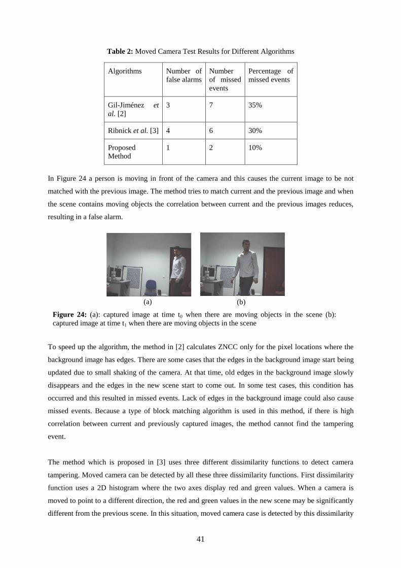
41
Table 2: Moved Camera Test Results for Different Algorithms
Algorithms Number of
false alarms
Number
of missed
events
Percentage of
missed events
Gil-Jiménez et
al. [2]
3 7 35%
Ribnick et al. [3] 4 6 30%
Proposed
Method
1 2 10%
In Figure 24 a person is moving in front of the camera and this causes the current image to be not
matched with the previous image. The method tries to match current and the previous image and when
the scene contains moving objects the correlation between current and the previous images reduces,
resulting in a false alarm.
To speed up the algorithm, the method in [2] calculates ZNCC only for the pixel locations where the
background image has edges. There are some cases that the edges in the background image start being
updated due to small shaking of the camera. At that time, old edges in the background image slowly
disappears and the edges in the new scene start to come out. In some test cases, this condition has
occurred and this resulted in missed events. Lack of edges in the background image could also cause
missed events. Because a type of block matching algorithm is used in this method, if there is high
correlation between current and previously captured images, the method cannot find the tampering
event.
The method which is proposed in [3] uses three different dissimilarity functions to detect camera
tampering. Moved camera can be detected by all these three dissimilarity functions. First dissimilarity
function uses a 2D histogram where the two axes display red and green values. When a camera is
moved to point to a different direction, the red and green values in the new scene may be significantly
different from the previous scene. In this situation, moved camera case is detected by this dissimilarity
(a)
(b)
Figure 24: (a): captured image at time t0 when there are moving objects in the scene (b):
captured image at time t1 when there are moving objects in the scene

42
function. There are some cases in the test scenarios which are detected by this way. In the second
dissimilarity function, another 2D histogram calculation is done. This histogram is sensitive to
illumination changes. Mostly, moved camera view isn‟t detected by this function but, some of the false
alarms observed to be caused by this function. The last dissimilarity function uses a one dimensional
histogram where the values are calculated according to the gradient direction of the pixels. This
function is used to detect some moved camera tampering cases. When camera view is moved, some of
the pixels in the scene are seen as moving and the histogram differs significantly.
In the proposed method, we compare the background image to a delayed background image to detect
the moved camera view. When a camera is moved to reflect a different view, the background starts to
update. If the difference between the updated background and the delayed background is higher than a
threshold, an alarm is triggered by this method to indicate the movement of the camera. There are
some cases that moving objects enter to or leave the adaptive background image. In these cases, the
background image will be different than the delayed background image, and if the amount of
difference is greater than the threshold a false alarm is generated. In Figure 25, a person is studying in
the scene at time t0 and because he is in the scene for several minutes, he is also seen in the
background image and in the delayed background image. When he leaves the scene, the background
image starts updating. At time t1, the person disappears from the background image. At this time,
background image is different than the delayed background image. Our method doesn‟t generate false
alarm for this case because the difference between background and delayed background image is not
enough for an alarm. However, if the moving object covers most of the view, which is not a likely
scenario in real life, or if the sensitivity increased by updating the threshold, a false alarm could be
raised by this method.
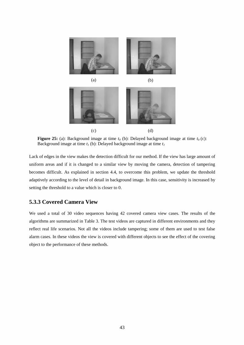
43
Lack of edges in the view makes the detection difficult for our method. If the view has large amount of
uniform areas and if it is changed to a similar view by moving the camera, detection of tampering
becomes difficult. As explained in section 4.4, to overcome this problem, we update the threshold
adaptively according to the level of detail in background image. In this case, sensitivity is increased by
setting the threshold to a value which is closer to 0.
5.3.3 Covered Camera View We used a total of 30 video sequences having 42 covered camera view cases. The results of the
algorithms are summarized in Table 3. The test videos are captured in different environments and they
reflect real life scenarios. Not all the videos include tampering; some of them are used to test false
alarm cases. In these videos the view is covered with different objects to see the effect of the covering
object to the performance of these methods.
(a)
(b)
(c)
(d)
Figure 25: (a): Background image at time t0 (b): Delayed background image at time t0 (c):
Background image at time t1 (b): Delayed background image at time t1

44
Table 3: Covered Camera Test Results for Different Algorithms
Algorithms Number
of false
alarms
Number of
missed
events
Percentage of missed
events
Aksay et al. [1] 7 7 16,7%
Gil-Jiménez et al. [2] 14 5 11,9%
Gil-Jiménez et al. [2]
(block based)
28 0 0%
Ribnick et al. [3] 10 3 7,1%
Proposed Method 4 2 4,8%
In [2], an entropy value is calculated and low entropy values are used to infer covered camera view.
When an object covers the lens of the camera, the objects in the scene will no longer be visible, and
the pixels in the background image disappear. In this situation, the proportion of black pixels in the
background image increases. In Figure 26, we show the background image and the change in the
entropy of this background image over time when the camera view is covered. In Figure 26(a), the
background image at time t0 is showed where the camera view is not covered. As you see from the
graphic, the entropy value is higher at time t0. When the camera view is covered at time t1 which is
shown in Figure 26(b), the edges in the background image starts disappearing. Loss of edges in the
background image causes the entropy value to decrease.
Moving objects which are covering the edges in the background image has caused false alarms. Such
objects change the pixels in the background image and the entropy is affected. The method in [2] also
has an alternative method for partial camera occlusions. In this method, image is divided into blocks
and entropy is calculated for each block separately. If one of the entropy values is lower than
previously calculated entropy, an alarm is triggered. Even though this increases the true alarm
detection rate, as the entropy of individual blocks are affected significantly by moving objects, it
generates considerably more false alarms and has the highest false alarm rate.

45
As we explain in section 4.4, we use a method similar to the one proposed in [1] with some
modifications. As seen from the results, the false alarm rate is lower in the proposed method than this
method. This method compares the maximum values of the histograms which are calculated using the
current and background image. However, there have been some test cases that an object enters the
scene and the maximum value in the current image‟s histogram significantly differs. In these cases,
false alarms are generated by this method.
The method in [3] uses 2 functions to detect covered camera view. When a camera view is covered,
the red and green objects in the scene become invisible. This change in the scene causes the 2D red
and green values histogram to change significantly. The first function in this method is used to detect
covered camera view. Another function which is used to detect this type of tampering is histogram
L1R difference. In this function another 2D histogram is calculated which is sensitive to changes in
illumination. Because the illumination in the scene changes when camera view is covered, this
function detects tampering. Figure 27 shows the change of these 2D histograms when the camera view
is covered.
Because the histograms in method [3] are sensitive to color and illumination changes, moving objects
in front of the camera and some illumination changes caused by sun light flickers are marked as
camera tampering. False alarms which are generated by this method are caused by these conditions.
(a)
(b)
(c)
Figure 26: (a): Background image which belongs to a non covered view at time t0 (b):
Background image of the covered view at time t1 (c): Entropy graphic
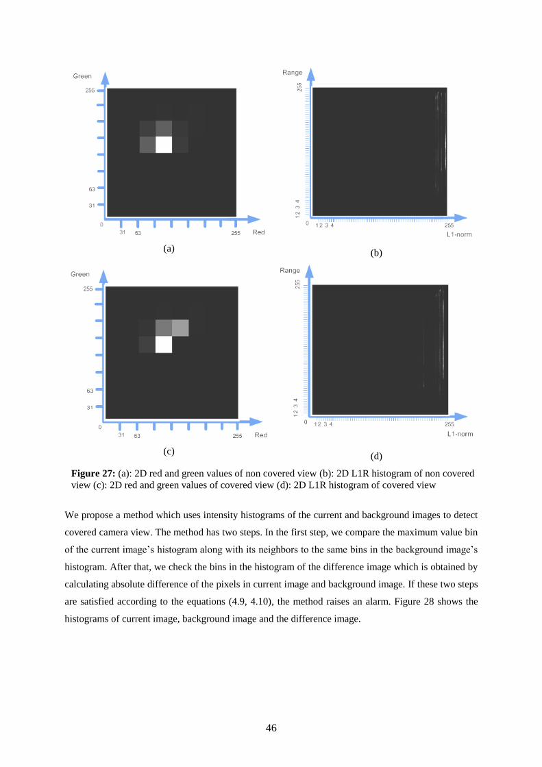
46
We propose a method which uses intensity histograms of the current and background images to detect
covered camera view. The method has two steps. In the first step, we compare the maximum value bin
of the current image‟s histogram along with its neighbors to the same bins in the background image‟s
histogram. After that, we check the bins in the histogram of the difference image which is obtained by
calculating absolute difference of the pixels in current image and background image. If these two steps
are satisfied according to the equations (4.9, 4.10), the method raises an alarm. Figure 28 shows the
histograms of current image, background image and the difference image.
(a)
(b)
(c)
(d)
Figure 27: (a): 2D red and green values of non covered view (b): 2D L1R histogram of non covered
view (c): 2D red and green values of covered view (d): 2D L1R histogram of covered view
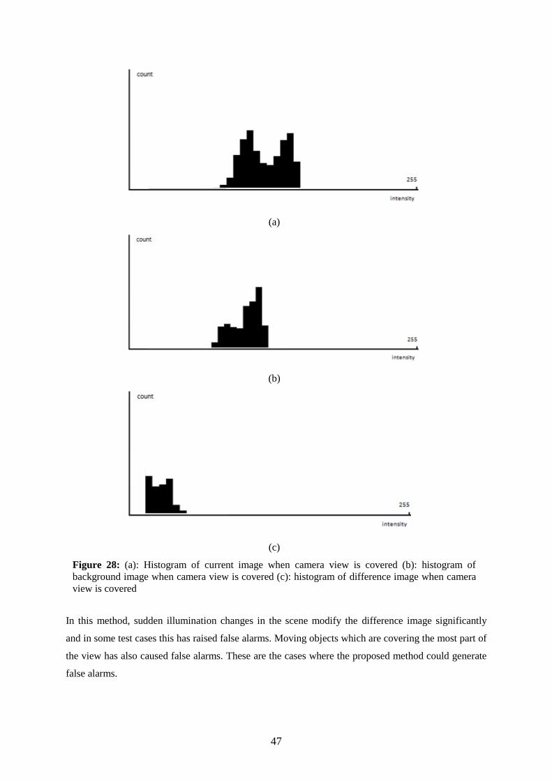
47
In this method, sudden illumination changes in the scene modify the difference image significantly
and in some test cases this has raised false alarms. Moving objects which are covering the most part of
the view has also caused false alarms. These are the cases where the proposed method could generate
false alarms.
(a)
(b)
(c)
Figure 28: (a): Histogram of current image when camera view is covered (b): histogram of
background image when camera view is covered (c): histogram of difference image when camera
view is covered
48
Sudden illumination changes are a shortcoming of our camera tampering detection algorithms. The
performances of these algorithms are affected when the amount of light in the environment changes
suddenly. Our test cases include this kind of events and in these test cases we see many false alarms
and a few missed events. To overcome this problem, an edge correspondence check may be applied.
Edge correspondence check is used to check that if a camera still is or is not monitoring the same
scene. If a camera viewing the same scene the edges in the background image and in the current
images should be in the same locations. If a sudden illumination change is occurred, camera still views
the same scene. By confirming that the camera is viewing the same scene we can distinguish
tampering cases from sudden illumination changes. To find number of corresponding edge pixels, we
can use the following equation.
𝐸𝑐𝑜𝑟𝑟𝑒𝑠𝑝𝑜𝑛𝑑𝑖𝑛𝑔 =
𝐸𝑐𝑜𝑟𝑟𝑒𝑠𝑝𝑜𝑛𝑑𝑖𝑛𝑔 + 1 , 𝑖𝑓 𝐼𝑛 𝑥,𝑦 − 𝐵𝑛 𝑥,𝑦 < 𝑇5
𝐸𝑐𝑜𝑟𝑟𝑒𝑠𝑝𝑜𝑛𝑑𝑖𝑛𝑔 , 𝑖𝑓 𝐼𝑛 𝑥,𝑦 − 𝐵𝑛 𝑥,𝑦 ≥ 𝑇5
(5.1)
where Ecorresponding is the number of corresponding edge pixels. (x,y) is the pixel positions where edges
exist in the current image and Th5 > 1 is the threshold value. When Th5 is set to a value which is closer
to one the sensitivity is increased. After finding the number of corresponding edge pixels, we may use
the following equation to find whether the camera is viewing the same scene or not.
𝐸𝑐𝑜𝑟𝑟𝑒𝑠𝑝𝑜𝑛𝑑𝑖𝑛𝑔 > 𝑇6𝐸𝑡𝑜𝑡𝑎𝑙 (5.2)
In this equation Etotal is the number of pixels where there are edges in the current image and 0<Th6<1
is the threshold value. To increase the sensitivity we set the threshold value which is closer to 1.
Another method which may be applied to reduce false alarm rate when sudden illumination change is
occurred may be normalizing all the pixels of the images according to the average light in the images.
If we subtract a proportion of average pixel value from all the pixels, the values of the pixels in the
images will be similar when a sudden illumination change is occurred. When the level of light in the
images is high or low, normalized images will be very similar. Because these normalized images is
more stable against sudden illumination changes, the number of false alarms or missed events may be
reduced by using these images in the camera tampering detection algorithms. This process can be
thought as preprocessing of camera tampering detection algorithms and it is showed in the following
equation:
𝐼𝑛𝑜𝑟𝑚𝑎𝑙𝑖𝑧𝑒𝑑 (𝑥,𝑦) = 𝐼(𝑥 ,𝑦) − 𝑃𝜇 (5.3)

49
where Inormalized(x,y) is the normalized pixel value at pixel position (x,y), and I(x,y) is the pixel
value of input image at position (x,y). µ is the mean pixel value of image I and P is the
proportion value.

50
CHAPTER 6
CONCLUSIONS AND FUTURE WORK
In this thesis, we propose new algorithms to detect three types of camera tampering which are camera
defocusing, camera movement and covering of a camera view. The algorithms are based on an
adaptive background estimation technique which uses a threshold mechanism to identify moving
objects. The thresholds are adaptively updated over time in accordance with the moving pixels in the
scene. For detecting defocused camera view, high frequency components of current image and
background image are compared. When camera view is defocused, the edges in the current image are
degraded which decreases the high frequency components of the current image. To acquire high
frequency components of the images, Fourier transform is applied to the images and then a Gaussian
window is used to discriminate high frequency values from the low frequencies. While we
experimenting this method, we realized that the moving objects in the scene can significantly change
high frequency data of current image which results in false alarm. To overcome this problem, we
propose an extension of this method which calculates high frequency data for only non moving
regions in the current and background image. For camera moving, we propose a method which
compares the background image to a delayed background image and the number of different pixels is
used to determine whether the camera is moved to a different direction. For camera covering, we
propose a method which checks the histograms of current, background and difference image. The
difference image is obtained by taking absolute difference between current and background image. In
the first step of this method, we compare the maximum value bin of the current image‟s histogram
along with its neighbors to the same bins in the background image‟s histogram. In the second step of
the method, the values in the histogram of difference image are analyzed to check whether or not a
significant percentage of the values are located near the black end.
We evaluated the proposed algorithms using a variety of camera tampering scenarios as well as 4
typical video surveillance footages not containing any tampering events totaling approximately 14
minutes from i-LIDS dataset [22]. Our results show that the proposed methods have low false alarm

51
rates and more favorable true alarm rates in defocused camera view, moved camera and covered
camera view cases compared to the other algorithms. In the defocused camera case, 2 different
methods are proposed. Both methods have missed same tampering events, but the first one generates
significant number of false alarms while the second one generates fewer false alarms. We have
decreased the number false alarms by block based processing to account for moving objects in the
scene.
The test videos include few sudden illumination changes which could potentially cause false alarms.
Even though not a likely scenario -considering the placement of real life CCTV cameras-, large
objects moving in front of the camera and covering most of the view could increase the number of
false alarms.
All the methods which aim to detect tampered camera view based on the same approach that, newly
captured images are compared to the older ones and if there is significant difference an alarm case is
generated. In this study, we also based on the same approach and proposed new techniques for
detecting camera tampering. We have evaluated our approach with a set of videos and compared to the
other methods in the literature. As seen from the test results, false alarm rate and number of missed
tampering events is lower than the other methods. We hope that this study will help researchers to
develop new solutions to similar problems in video surveillance research area.
In the future, the proposed camera tampering detection algorithms may be enhanced by making them
robust against sudden illumination changes. In Chapter 5 some methods which may be used reduce
effect of sudden illumination changes are explained. These methods may be implemented and tested to
evaluate their performance.
These algorithms may be adapted to work in different platforms in the future. For example, the
algorithms may work in embedded systems and by this way, all the checks against camera tampering
may work on a single camera. This system may also be integrated into existing security systems. For
example, referring to the Mexico prison escape which is explained in chapter 1, if there had been an
integrated system where the camera tampering detection algorithms controlled the doors of that
section of the prison, the doors would be able to be lock automatically and the escape may have been
prevented.

52
REFERENCES
[1] Aksay Anıl, Temizel Alptekin and Çetin A. Enis., "Camera Tamper Detection Using Wavelet
Analysis for Video Surveillance." IEEE International Conferance on Video and Signal Based
Surveillance, September 2007.
[2] Gil-Jiménez P., Lopez-Sastre R., Siegmann P., Acevedo-Rodriguez J., Maldonado-Bascon S.,
"Automatic Control of Video Surveillance Camera Sabotage." s.l. : J. Mira and J.R. Alvarez (Eds.):
IWINAC 2007, 2007.
[3] Ribnick Evan, Atev Stefan, Masoud Osama, Papanikolopoulos Nikolas, Voyles Richard, "Real-
Time Detection of Camera Tampering." s.l. : IEEE International Conferance on Video and Signal
Based Survelliance, 2006.
[4] Piccardi, Massimo., "Background Subtraction Techniques: a review." s.l. : IEEE International
Conference on Systems, Man and Cybernetics, 2004. 0-7803-8566.
[5] Sen-Ching, S. Cheung and Chandrika, Kamath., "Robust techniques for background subtraction in
urban traffic video." San Jose : Video Communications and Image Processing, SPIE Electronic
Imaging, January 2004. UCRL-JC-153846-ABS, UCRL-CONF-200706 .
[6] Wren, C., Azarhayejani, A., Darrell, T. A.P., "Pfinder: real-time tracking of the human." s.l. : IEEE
Trans. on Patfern Anal. and Machine Intell. vol. 19, no. 7, pp. 78g785, 1997.
[7] , Background subtraction, part 1: MATLAB models. DSP DesignLine. [Online] [Cited: 12 May
2009.]
http://www.dspdesignline.com/howto/210000460;jsessionid=KGBUUEXZDIKJ0QSNDLRCKHSCJ
UNN2JVN?pgno=3.
[8] Stauffer, C. and Grimson, W.E.L., "Adaptive background mixture models for real-time tracking."
s.l. : IEEE CVPR 1999, pp. 24&252, June 1999.

53
[9] Elgammal, A., Harwood, D. and Davis, L.S., "Non parametric model for background subtraction."
June 2000. Proc. ECCV 2000. pp. 751-767.
[10] Han, Bohyung, Comaniciu, Dorin and Davis, Larry., "Sequential Kernel Density Approximation
Through Mode Propagation:applications to background modelling." January 2004. Proc. Asian Conf.
on Computer Vision.
[11] Seki, Makito, et al., "Background Subtraction based on Cooccurrence of Image Variations."
2003. IEEE Computer Society Conference on Computer Vision and Pattern Recognition (CVPR‟03),
1063-6919/03. pp. 65-72.
[12] Xu, Zhifei, Shi, Pengfei and Yu-Hua Gu, Irene., "An Eigenbackground Subtraction Method Using
Recursive Error Compensation." [book auth.] Lecture Notes in Computer Science. Advances in
Multimedia Information Processing - PCM 2006. s.l. : Springer Berlin / Heidelberg, 2006, pp. 779-
787.
[13] Collins R.T., Lipton A.J., Kanade T., Fujiyoshi H., Duggins D., Tsin Y., Tolliver D., Enomoto N.,
Hasegawa O., Burt P., Wixon L., A system for video surveillance and monitoring: VSAM final report.
s.l. : Carnegie Mellon University, May 1998. Technical Report CMURI-TR-00-12.
[14] Fridrich, Jiri., "Image Watermarking for Tamper Detection." 1998. Proc. of ICIP, vol.2. pp. 404-
408.
[15] Roberts, D.K., "Security Camera Video Authentication." October 2002. Digital Signal Processing
Workshop and the Signal Processing Education Workshop. pp. 125-130.
[16] Lim, Suk Hwan, Yen, Jonathan and Wu, Peng., "DETECTION OF OUT-OF-FOCUS DIGITAL
PHOTOGRAPHS." January 2005. Imaging Systems Laboratory, HP Laboratories Palo Alto.
[17] Nam, Jeho and Tewfik, Ahmed H., "Detection of Gradual Transitions in Video Sequences."
August 2005. IEEE TRANSACTIONS ON MULTIMEDIA, VOL. 7, NO. 4. pp. 667-679.
[18] Heng, Wei Jyh and Ngan, King N., "Integrated Shot Boundary Detection using Object-based
Technique." October 1999. Proceedings of International Conference on Image Processing, vol. 3. pp.
289-293.
[19] Tomassi, Carlo and Kanade, Takeo., "Shape and Motion from Image Image Streams Under
Orthography: a Factorization Method." September 1993. IJCP, vol. 9, no. 2. pp. 864-884.

54
[20] Weng, Juyang, Ahuja, Narendra and Huang, Thomas S., "Optimal Motion and Structure
Estimation." September 1993. IEEE TRANSACTIONS ON PATTERN ANALYSIS AND
MACHINE INTELLIGENCE, VOL. 15, NO. 9. pp. 864-884.
[21] Harasse, S., Bonnaud, L., Caplier, A., Desvignes, M., "Automated camera dysfunctions
detection." March 2004. Image Analysis and Interpretation, 6th IEEE Southwest Symposium. pp. 36-
40.
[22] i-LIDS dataset for AVSS 2007. [Online] [Cited: 13 March 2009.]
http://www.elec.qmul.ac.uk/staffinfo/andrea/avss2007_d.html.
[23] OpenCV Documentation and FAQs. [Online] [Cited: 13 March 2009.]
http://opencvlibrary.sourceforge.net/.
[24] Gary, Bradski and Kaehler Adrian., Learning OpenCV. s.l. : O'Reilly, September 2008. 978-0-
596-51613-0.
Recommended