AD-A243 753 :0I flllihIi MI 111 IDil! 1111 III I!' i:1I I cEECTE
SDEC 2 41991lJ
Ai in
DEPARTMENT OF THE AIR FORCE
AIR UNIVERSITY
AIR FORCE INSTITUTE OF TECHNOLOGY
Wright-Patterson Air Force Base, Ohio
IN~eo~~ DIO tABEli
AFIT/GE/ENG/91D-23 _______________________-
lDist ibmtlvi ./IAv.labilitr Coies
Tavil alqd/orDi3t Ispecial
GABOR SEGMENTATION OF IGH RESOLUTIONSYNTHETIC APERTURE RADAR IMAGERY
THESIS
Michael Alan HazlettCaptain, USAF
'AFIT/GE/ENG/91D-23
Approved for public release; distribution unlimited
91-1900,//!!liii/l~ t °llil111t,
AFIT/GE/ENG/91D-23
GABOR SEGMENTATION OF IGH RESOLUTION
SYNTHETIC APERTURE RADAR IMAGERY
THESIS
Presented to the Faculty of the School of Engineering
of the Air Force Institute of Technology
Air University
In Partial Fulfillment of the
Requirements for the Degree of
Master of Science in Electrical Engineering
M~ichael Alan H-azlett, B.S.B.
Captain,. USAF
December, 1991
Approved for public release; distribution unlimited

Acknowledgments
j wish to thank all of those people who made this research possible. First,
I would like to thank my advisor, Dennis Ruck, for all his advice and patience in
those times when things weren't going as planned. Second, I would like to thank
Steve Rogers for his classes on pattern recognition. These classes peaked my interest
in the area of pattern recognition and led to this research. Finally, I would like to
thank my wife, Carol, and my children, Katie, Alex and Emily for all their love and
support during the stressful time of preparing this research.
Michael Alan Hazlett
Table of Contents
Acknowledgments . ....... ....
Table of Contenits........ .. .. .. .. .. .. .. .. .. .. .. .. .. . . ....
List of Figures .. .. .. .. ... ... ... .. ... ... ... .. ... ... vi
List of Tables .. .. .. .. .. ... ... .. ... ... ... .. ... ..... viii
Abstract .. .. .. .. .. ... .. ... ... ... .. ... ... ... ..... ix
1. Introduction. .. .. .. .. .. ... ... .. ... ... ... .. .....
1.1 General .. .. .. .. .. ... ... ... .. ... ...... 1
1.2 Background .. .. .. .. .. ... ... ... .. ... .... 2
1.3 SAR lImagery .. .. .. .. .. ... .. ... ... ... ... 2
1.4 Problem Statement .. .. .. .. .. .. ... ... .. .... 2
1.5 Research Objectives. .. .. .. .. ... .. ... ... ... 2
1.6 Definitions .. .. .. .. ... ... .. ... ... ... ... 4
1.7 Scope .. .. .. .. .. ... ... ... ... .. ... .... 4
1.8 General Approach. .. .. .. .. .. .. ... ... .. .... 4
1.9 Overvi-w . .. .. .. .. ... ... .. ... ... ... ... 5
11. Literature Review. .. .. .. .. .. .. ... ... ... ... .. .... 6
2.1 Introduction. .. .. .. .. .. .. ... ... ... .. .... 6
2.2 Gabor Filters .. .. .. .. .. ... .. ... ... ... ... 6
2.2.1 Biological Motivation .. .. .. .. .. .. ... ... 6
2.2.2 Gabor Usage .. .. .. .. .. ... ... ... ... 82.3 Radial Basis Functions. .. .. .. .. .. ... .. ... ... 9
2.4 Summary .. .. .. .. .. ... ... .. ... ... ..... 11
iii
Page
III. Methodology ....... ............................... 12
3.1 SAR Image Preprocessing ...................... 12
3.2 Gabor Filter Generation ........................ 12
3.3 Gabor Coefficient Calculation ................ 12
3.4 Gabor Filter Selection ........................ 13
3.5 RBF Training.. .............................. 13
3.6 Image Segmentation .......................... 14
3.7 Summary ................................. 14
IV. Results ......................................... 15
4.1 SAR Imagery ............................... 15
4.1.1 M85F27 ............................ 15
4.1.2 M85F28 ............................. 15
4.1.3 M85F30 ............................ 15
4.1.4 M98F07 ............................ 15
4.1.5 M98FO8 ............................ 19
4.1.6 M98F09 ............................. 19
4.1.7 M98F10. .............................. 19
4.2 Correlation Coefficient Calculation ............. 19
4.3 Gabor Filter Selection Using Fourier Technique ...... ... 20
4.4 Histogram mi ug Technique ...................... 21
4.5 RBF Training.. .............................. 28
4.6 Training Results ........................... .35
4.7 Segmentation Results ......................... 35
4.8 Median Filtering .............................. 37
V. Conclusions and Recommendations ....................... 40
5.1 Introduction ..... .......................... 410
5.2 Further Research ............................ '10
;v
Page
Appendix A. The Gabor Representation...................... 42
Appendix B. Other RBF Segmentation Results. .. .. .. .. .. ...... 47
Appendix C. Program Listinas .. .. .. .. .. ... ... ... .. .... 51
0.1 correlate. .. .. .. ... ... ... ... .. ... ...... 51
C.2 rebuilcl.c. .. .. .. .. .. ... ... ... ... .. ..... 58
Bibliography. .. .. .. ... ... ... .. ... ... ... ... .. ..... 63
Vita. .. .. .. .. ... ... ... ... .. ... ... ... ... .. ..... 65

List of Figures
Figure Page1. Sample ADTS SAR Imagery: Mission 85, Frames 27-30 .......... 3
2. Comparison of 2-D Simple Cell Receptive Fields to Gabor Functions 7
3. Two Layer Radial Basis Function ......................... 11
4. Mission 85, Frame 27, 1114 Polarization ..................... 16
5. Mission 85, Frame 28, 1111 Polarization ..................... 16
6. Mission 85, Frame 29, -1-1 Polarization ..................... 17
7. Mission 85, Frame 30, H-I Polarization ..................... 17
8. Mission 98,Frame 07, 11H Polarization ..................... 18
9. Mission 98, Frame 08, IH Polarization ..................... 18
10. Mission 98, Frame 09, HH1- Polarization ..................... 19
11. Mission 98, Frame 10, 1111 Polarization ..................... 20
12. Typical Power Spectrum of 16 x 16 Window of Tree Region ..... 22
13. Typical Power Spectrum of 16 x 16 Window of Grass Region . . .. 23
14. Typical Power Spectrum of 16 x 16 Window of Shadow Region . . . 24
15. Histogram of Tree Region Filter Frequency Response, 32 Pixel Window 25
16. Histogram of Grass Region Filter Frequency Response, 32 Pixel Window 26
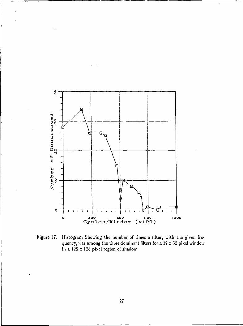
17. Histogram of Shadow Region Filter Frequency Response, 32 pixel Win-dow ..... . ...... .............................. 27
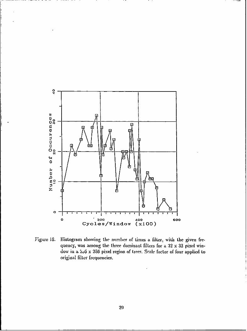
18. Histogram of Tree Region Filter Frequency Response, 32 Pixel WVindow,
Scale Factor 4 ....... .............................. 29
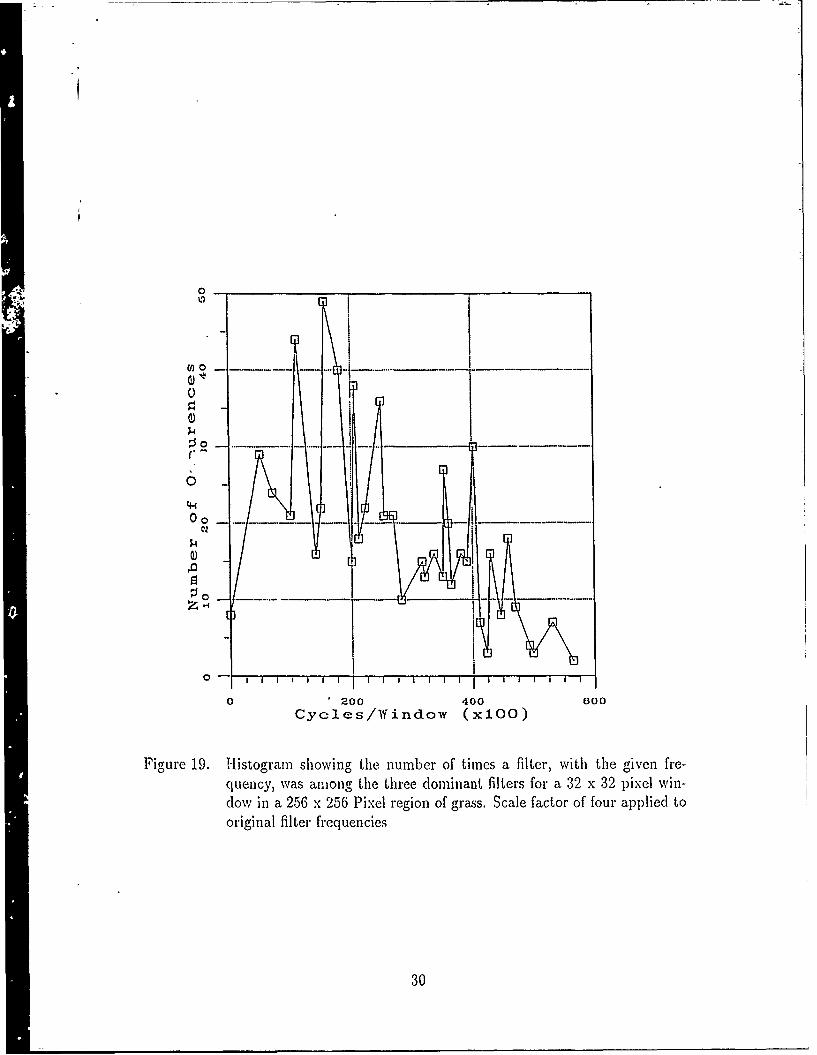
19. Histogram of Grass Region Filter Frequency Response, 32 Pixel Win-
dow, Scale Factor 4 ....... ........................... 30
20. Histogram of Shadow Region Filter Frequency Response, 32 pixel Win
dow, Scale Factor 4 ....... ........................... 31
21. Histogram of Tree Region Filter Frequency Response, 16 Pixel Window,
Scale Factor 2 ....... .............................. 32
vi
Figure Pg
22. Histogram of Grass Region Filter Frequency Response, 16 Pixel Win-
dow, Scale Factor 2 .. .. .. ... .. ... ... ... ... .. .... 33
23. 1-istogram of Shadow Region Filter Freqiuency Response. 16 pixe IWin-
dow, Scale Factor 2 .. .. .. ... ... .. ... ... ... .. .... 34
24. Mission q , Frame 07 Hand Segmented. .. .. .. .. ... .. ..... 36
25. Mission 98, Frame 07 RBF Segmented. .. .. .. .. ... ... .... 36
26. IMission 98, Frame 10 RBF Segmented .. .. .. .. .. ... ... ... 38
27. Mission 98, Frame 07 RBF Segmented, 5 einFle.....39
28. Three Layer Net for Finding Optimal Coefficients. .. .. .. .. .... 43
29. Mission 85, Frame 27, RBF Segmentation, 5 x 5 Median Filter .. . . 47
30. Mission 85, Frame 28, RI3F Segmentation, 5 x .5 IMedian Filter .. . . 48
31. Mission 85, Frame 29, R13F Segmentation, 5 x 5 Median Filter. .. 48
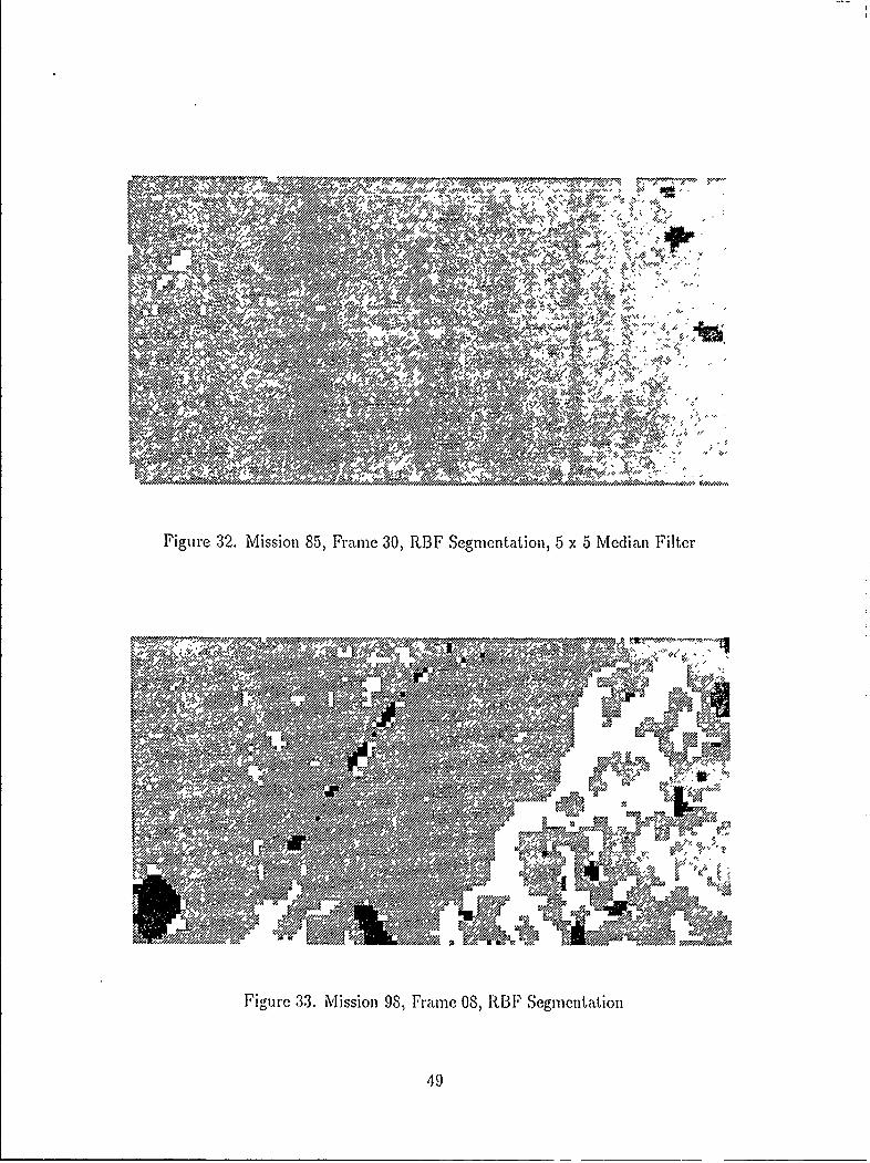
32. Mission 85, Frame 30, RBF Segmentation, 5 x 5 Median Filter .. . . 49
33. Mission 98, Frame 08, RBF Segmentation .. .. .. .. ... .. .... 49
34. IMission 98, Framne 09, RI3F Segmentation, 5 x 5 Median Filter .. . 50
vii

List of Tables
'1Able Page1. SAR Imagery Frequency Analysis .. .. .. .. .. .. ... .. . .... 21
2. Selected Filters for Image Processing .. .. .. .. .. ... .. . .... 28
viii
APIT/GE/ENG/9 ID-23
A bstract
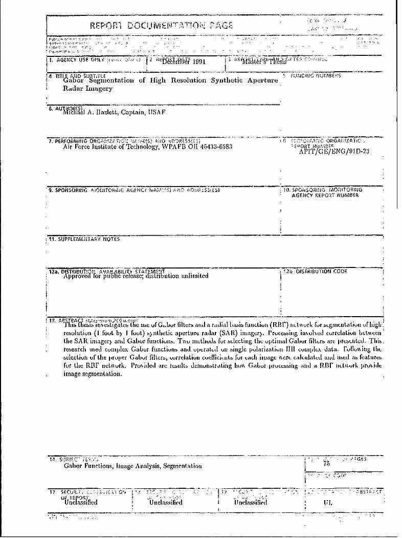
This thesis investigates the use of Gabor filters and a radial basis function
(RBF) network for segmentation of high resolution (1 foot by I foot) synthetic
ap)ert ure radar (S AR) iminagery. Processing inuvolvedi correladion between tile SA R
imnagery and Gabor functions. Two methods for selecting the op)timal Gabor filters
are p~resented. This research used complex Gabor functions and operated oil single
lpolarization 1-11-1 complex data. Following the selection of the proper Gabor filters,correlation coefficients for each image were calculated and uscel as features for the
RBF network. PrQviclec are results demonstrating how Gabor p)rocessinlg and atR3
network provide image segmentation.
Uix-
GABOR SEGMENTATION OF 11IGH RESOLUTION
SYNTHETIC APERTURE RADAR EIAGERY
I. Introduction
1. 1 General
Research in pattern recognition at the Air Force Institute of Technology (A FIT)
has been working toward building an autonomous target recognizer (ATR). The
eventual goal is to incorporate this ATR in a missile capable to autonomously locate
and destroy a hostile target located within the missile's field of view.
To date, many techniques have been developed which provide a limited solution
to the problem of object or texture recognition by machines. Complete machine
recognition remains an unsolved problem. There currently exist machines capable
of limited recognition within a controlled environment. These exist in supermarkets
and industrial production lines. The environment for these machines often control
noise, object scale, orientation, and position so the features are easier to extract.
The development of a target recognizer is much more complex. These machines
will typically be housed in small spaces such as missiles. aircraft or spacecraft. In
addition, the environment will no longer be controllable thereby creating a whole
new set of processing problems. Thcrc will be conditions of extreme noise and
temperature along with limitations imposed by the processing spced of the computer
and the algorithms used.
The ability of a target recognizer to be able to pull out cultural items, such as
targets. requires obtaining good sensor data. Assuming that high quality sensor data
is available, then the three steps in the target recognition process are segmentation.
feature extraction and classification (12). Seginwntation places a label on each pixel
in an image and locates blobs of interest. Feature extraction computes a muuber of
features for each blob detected by segmentation. Classification assigas a label to an
input feature vector generated. This research will focus in on the first step of the
target recognition process.
1.2 Background
Previous work by Captain Albert L'Homme (6) used Gabor functions and
an Artificial Neural Network (ANN) to segment Synthetic Apeiure Radar (SAl,)
imagery. His approach correlated the image with a set of nine Gabor filters inthe frequency domain. He then used the coefficients of the Gabor filters as input
vectors to train a Radial Basis Function (RBF) to segment SAR images. The successrate he achieved in segmenting was better than 80%. However, his work had a
few limitations. First, only a limited set Gabor filters was used. Second, only
the magnitudes of the SAR data was used, therefore, all phase information was
lost. Finally, only a single polarization, horizontal-horizontal (11H), of the four
polarizations of data available was used. Any information contained in the other
polarizations was lost.
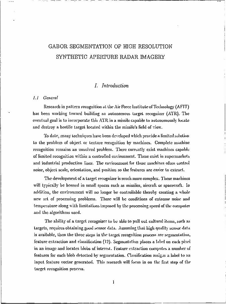
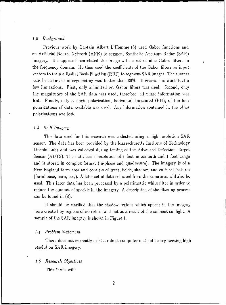
1.3 SAR Imagery
The data used for this research was collected using a high resolution SARsensor. The data has been provided by the Massachusetts Institute of Technology
Lincoln Labs and was collected during testing of the Advanced Detection Target
Sensor (ADTS). The data has a resolution of 1 foot in azimuth and 1 foot range
and is stored in complex format (in-phase and quadrature). The imagery is of a
New England farm area and consists of trees, fields, shadow, and cultural features
(farmhouse, barn, etc,). A later set of data collected from the same area will also beused. This later data has been processed by a polarimetric white filter in order toreduce the amount of speckle in the imagery. A description of the filtering processcan be found in (8).
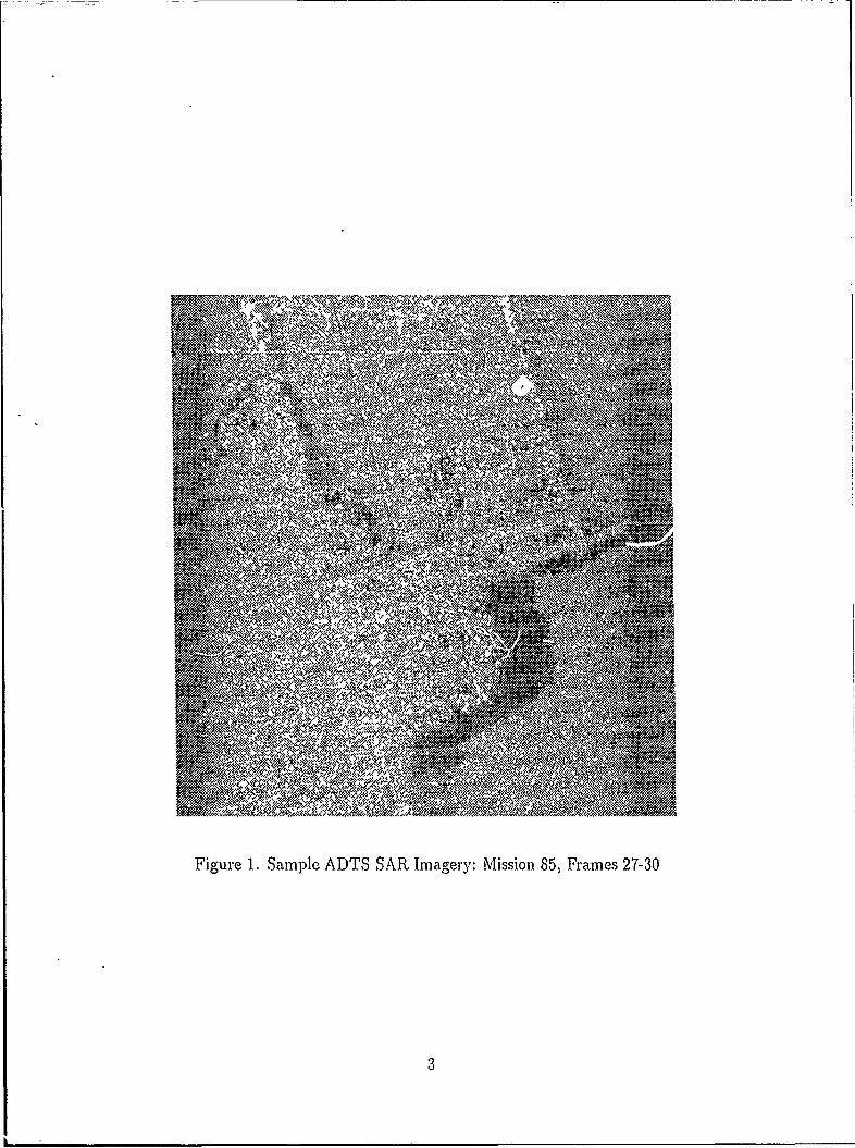
It should be clarified that the shadow regions which appear in the imagerywere created by regions of no return and not as a result of the ambient sunlight. A
sample of the SAR, imagery is shown in Figure 1.
1.4 Problem Statement
There does not currently exist a robust computer method for segmenting highresolution SAR imagery.
1.5 Research Objectives
This thesis will:
2
TM g
tMERE &E90 *0< i
MUN NO, Ma IN,
p4'
I I EelNIN R-W < BA.
'MR-, " 0-1-0-1MEMO
.sv >ggs0
gr,
wlknyano
"MUMW-M.Cy
MEe5p-M."
, NO"',M-
V-2.w'.
MI,
MN P2' W.
Figure 1. Sample ADTS SAR Imagery: Mission 85, Frames 27-30
3
e Search for an optimal set of Gabor functions associated with regions of trees,
fields, shadows, and culture through the use of histogramning and Fourier
techniques.
* Use the correlation coefficients from the optimal Gabor filters as inputs to an
ANN which ,vill segment the SAR imagery.
1.6 Definitionis
Segmentation is the process of dividing up a scene based on the image structure
to identify objects of interest from background regions.
Pattern recognition is the process of determining the correct identity of the
objects of interest segmented from an image.
Radial basis functions are a type of feedforward neural network that compute
by using neurons with local receptive fields. These neurons encode the inputs by
computing the closeness of the input to the center of their respective receptive fields.
(16:11- 133)
Correlation is a measure of similarity between two objects.
1.7 Scope
The major focus of this research will investigate which combinations of Gabor
filters will provide the best ANN input feature set in order to segment SAR imagery
into regions of trees, field, shadow, and culture.
1.8 General Approach
Initially, the work to be performed will include some 256 different variations of
the Gabor function used to process the complex SAR imagery. Next will be selection
of the optimal Gabor filters. Two methods for selecting the optimal filters will be
examined. The first method selects the optimal filters based upon the filters with
largest coefficient for a particular region type (trees, grass and shadow). The second
method, suggested by Bovik (2:63), will perform a Fast Fourier Transform (FFT) on
selected regions of the image and select the Gabor filters whose frequency response
matches with the two strongest peaks in the image power spectrum. The coefficients
from the selected filters will in turn be used as vectors to input into an ANN for the
purpose of training the ANN to segment other SAR imagery.
4

1.9 Overview
Chapter II presents a review of current literature applicable to Gabor filtering
and radial basis functions as related to segmentation of high resolution SAP. imagery.,
Chapter III presents methodology used for this research. Provided is a descrip-
tion of Gabor functions, techniques for determining the optimal Gabor functions, and
a description of the ANN used for image segmentation.
Chapter IV discusses the results and analysis of this research.
Chapter V presents conclusions and recommendations for further research.
II. Literature Review
2.1 Introduction
This chapter reviews literature found useful for application of Gabor filtering
and radial basis functions. The intent is to find techniques, within this literature,
which can be used for segmenting high resolution SARP imagery. In addition, the
literature will be used to show the validity of using Gabor filters and radial basis
functions combined as a method for segmenting SAR imagery.
2.2 Gabor Filters
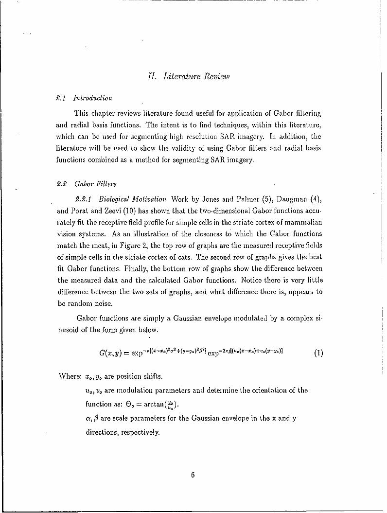
2.2.1 Biological Motivation Work by Jones and Palmer (5), Daugman (4),
and Porat and Zeevi (10) has shown that the two-dimensional Gabor functions accu-
rately fit the receptive field profile for simple cells in the striate cortex of mammalian
vision systems. As an illustration of the closeness to which the Gabor functions
match the meat, in Figure 2, the top row of graphs are the measured receptive fields
of simple cells in the striate cortex of cats. The second row of graphs gives the best
fit Gabor functions. Finally, the bottom row of graphs show the difference between
the measured data and the calculated Gabor functions. Notice there is very little
difference between the two sets of graphs, and what difference there is, appears to
be random noise.
Gabor functions are simply a Gaussian envelope modulated by a complex si-
nusoid of the form given below.
G(x, y) = exI) -I(xo)a+(v -y°)Pl exp- 2 -[(-(x - x)+vo(v- )] (1)
Where: x,, Yo are position shifts.
u,, v, are modulation parameters and determine the orientation of the
function as: Eo = arctan(y).
a, 0 are scale parameters for the Gaussian envelope in the x and y
directions, respectively.
7I'
2-D Recentive Field Ij. ,\\
j
2-D Gabor Functilon ,,
Difference
Figure 2. Comparison of 2-D Simple Cell Receptive Fields to Gabor Functions (5).The first row shows the measured two-dimensional response in simplecells of the cat visual cortex. The second row shows a set of "best fit"Gabor functions. The third row shows the residual error between theGabor functions and the measured responses.
7
Bovik (2), Daugman (3), Lu (7), have used Gabor functions to process differ-ent types of imagery and have found the Gabor filters able to distinguish between
textures in an image. Bovik stated,
The Gabor implementation effectively unifies the solution of the con-flicting problems of determining local textural structures (feCtures, tex-ture boundaries) and identifying th:e spatial extent of textures contribut-ing significant spectral information ... (2:71)
2.2.2 Gabov Usage Daugman made use of a comnplete set of Gabor filters touse for image segmentation. The filters were based on a window size of 32 x 32
pixels, but could be generalized to any window size. In addition, the windows usedwere overlapping windows rather than independent windows as used in the lpreviouseffort of L'Hinomme. The general equation for these Gabor filters is (3:1176):
G(x, y) = exp(-r - (y - zN)']) 'exp(-27,rj[7" + S-s]) (2)
Where: Al, N - window dimensions
a 2 - Gaussian scale constant
m, n - integers indicating location of window
r,s - integer, increments of spatial freqiency in the range
(-M/2 - 1, A'J/2) and (-N/2 - 1, TN?) respectively
The Gaussian space constant, a, determi,.c, .: i roll-off o," che Gaussian enve-lope. In this case a is set such that the value of the Gaussian envelope is 1/c at ±9pixels for a 32 pixel window size.
The frequency and rotati n of the filters is determined by r, s, M and N asfollows:
7-f =(3)
fy (4)
F = f ' (5)
E= arct,'.' f/,,If) (6)
Where: f. = frequency in the x dircc:,io:,
f7 = frequency in the y direction
F = frequency of the filter
0 = rotation of the filter
Daugman has also suggested a neural network to solve the problem of the non-orthogonality of Gabor functions w' a used az- a basis set. A description of the
network-and its operation is given in Appendix A.
Several efforts at AFIT have concentrated in the area of Gabor segmentationand filtering of both Infrared (IR) and SAR imagery. Work iL-complished by Kevin
Ayer (1) ivolved Gabor filtering of Forward-Looking Infrared (FLIR) imagery. Ayer
was .ble to successfully pick out targets, tanks, trucks, and jeeps, Trim the back-ground. Ayer's work was done via computer whie similar %,'.rk was done optically
by Christop,,.: Veronin (15). With correct selection of filters, Veronin was able to
pick out the targets from th background as well. In additon, Veronin was able tcoptically reproduce Bovik's texture discrimination. The latest work clone with Ga-bor filters for segmenting SAR imagery was done by Albert L'Itomme ab mentioned
in Section 1.2.
Since Gabor functions. are biologically motivated and have proven useful to
discriminate textures, these functions may be the way to front-eiid process imagery.
Since the human brain has a throughput rate of only about 50 bits/sec (9), a largereduction in the amount of input data has to be accomplished in order for the brainto accomplish the task of recognition. Gabor processing of imagery does reduce the
amount of data input and appears to provide a useful set of features for ami image
segmentation algorithm.
2.3 Radial Basis Functions
A Radial Basis Function network (RBF) is an ANN used to classify superviseddata. Instead of each neuron firing as the "ctu. of a liar or nonlinear function of it's
9

input, they each h:-ve an associated Gaussian receptive field The location and spread
of each receptive field are controlled by two parameters, the mean and the standard
dev;ation respectively. The are two methods avaiLbibe within Zahii-ak's code (17:4-
3) tW set the mean of the Gaussian receptive field. The first meth ,- ib to move the
centers of the Gaussians to the locations of clusters of the data (class average) in
the feature space and adjust thc spread of the Gaus,t)n to include co-lo, Itecd data
of the same output class. The second method is to set the mean of th( G"aussians
to de points in the input data. In addition, Zahirniak's code (17:4-4) als) allows
sever .1 methods to calculate the spread, o, of the Gaussian r( ;ceptie field. The
three methods aie scale sigma according to class interferencc-, - igma according to
P-neighbor distance, and set '(nia to a constant. For this res_.rch, centering the
Gaussians at class averages and scaling sigma according to class interference will be
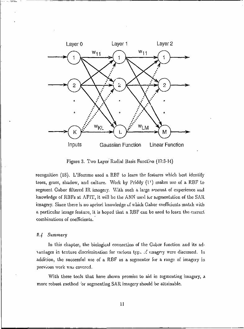
used. An example of a two-layer RBF is shown in Figure 3. The nodes of the output
layer comput a linear combination of out )uts from the hidden layer nodes. This
makes the output mapping for any single inlput pattern
Ym= i wfmyJj
1=1
and the output from the jdden layer nodes, yj is
Where: xk - k 4 component of the input pattern vector :
Wkl k 14h component of the weight vector
ok = the spreid in the k 'I direction.
The mean of the Gaussian receptive field for a RBF node is determined by its
iniput. weights. Shnce the weights Jetermine a vector in the feature space, this vector
locates the mean of the Gaussian in the feature space. The variance of the Gaussian
function controls how widely spread the function is; the larger the variance, the more
widely spread out it is the function within the feature space.
Daniel Zahirniak used RBF's to identify a radar by its transmitting charac-
teristics (17). In addition, lie also described the use o[ a RBF network for pattern
10
Layer 0 Layer 1 Layer 2
[°WKL wLM'°KL M
Inputs Gaussian Function Linear Function
Figure 3. Two Layer Radial Basis Function (17:3-14)
recognition (18). L'HiJomme used a RBF to learn the features which best identify
trees, grass, shadow, and culture. Work by Priddy (11) makes use of a RBF tosegment Gabor filtered IR imagey. With such a large amount of experience and
knowledge of RIBFs at AFIT, it will be the ANN used ur segmentation of the SARimagery. Since there is no apriori knowledge of which Gabor coefficients match with
a particular image feature, it is hoped that a R13F can be used to learn the correct
combinations of coefficients.
2.4 Summary
In this chapter, the biological connection of the Gabor function and its ad-xantages in texture discrimination for various tyl.. u'nagery were discussed. In
addition, the successful use of a RBF as a segmenter for a range of imagery in
previous work wa , covered.
With these tools that have shown )romise to aid in segmenting imagery, amore robust method -or segmenting SAR imagery should be attainable.
11
III. Methodology
This chapter will cover the methodologies used to segment the high resolution
SAR imagery. First, the preprocessing done to each SAR image will be shown.Second, will be a description of the slidin.g window and Gabor functions used. Third,
the method of computing the optimal Gabor coefficients will be explained. Fourth,
the implementation and training of a RBF to select the proper classification of the
input data will be covered. Finally, image segmentation will be discussed.
3.1 SAR Image Preprocessing
Each SAR image is composed of four frames of dimension 512 x 2048 pixels
resulting in an image size of 2048 x 2048 pixels. These frames contained low return
areas on both the left and right side of the image due to roll-off of the main beam
of the radar as can be seen in the dark areas in Figure 1. The radar was calibrated
for the center of the main beam which corresponds to the center of the image. Thus,
the center 1024 pixels from each frame were used for this research.
In an attempt to normalize the data from different missions, each reduced (512x 1024) frame was Fourier transformed via an FFT, the DC component was set to
zero, and the frame was inverse transformed.
3.2 Gabor Filter Generation
The initial set of Gabor filters used will be those based upon filters suggestedby Daugman as mentioned in Section 2.2.2. These form a complete set of Gabor
filters for a window size of 32 x 32 pixels. Using the same Equation 2, a complete set
of Gabor filters for a window size of 16 x 16 pixels w~il be generated. In the case of
a 32 pixel window size, this will result in 2.56 filters. In the other case of a 16 pixelwindow, the result will be 64 filters.
3.3 Gabor Coefficient Calculation
The Gabor coefficients for the SAR imagery will be computed by correlating a
set of complex Gabor filters with the complex SAR image. The correlation will be
performed in the space domain through the use of a sliding window. The window
12
size will be varied from a starting size of 32 x 32 pixels to a size of 16 x 16 pixels.
The window will start in the upper left-hand corner with its center placed at the
same location in the image as in the window. For example, for a window size of 32
x 32 pixels the starting location would be at pixel location (16,16) on the image.
This also corresponds to the center of the window which is at (16,16). The window
will the be moved across the image in steps of 1 the window size both horizontally
and vertically. At each location, the Cabor filter will be correlated with the image
yielding a set of correlation coefficient.
3.4 Gabor Filter Selection
Two methods will be used to find the optimal set of Cabor filters for use in
the training of the R13F. The first method suggested by Bovik (2:63) is to compute
the power spectrum of the image and select the two highest peaks and select the
Gabor filter associated with that location in the spatial frequency domain. The
second method involves histogramming of the Gabor filter coefficients. Coefficients
will be calculated for windows containing only a known region of trecs, grass, and
shadow. For cach window the three filters having the largest magnitude coefficient
will be tallied. After all the windows have been processed, the final counts will be
histogrammed. The filters having the largest number of occurrences will then be
used as the set of filters to process entire SAR images with.
3.5 RBF Training
The radial basis function to be used will be implemented using the neural
network software developed by Zahirniak (17). The software allows the user to
choose the entire architecture of the network and select from among several training
methods for establishing the network weights.
The number of cluster centers will be varied in order to find the optimal num-
ber. The limitation to this RBF is that the number of training vectors is limited to
200. This limitation is imposed by the size of the matrix inversion routine imple-
mented by Zahirniak.
All input data will be statistically normalized. This )rocedure involves calcu-
lating the mean and standard deviation for each feature of the input vector. The
data. for each feature is then normalized according to a Gaussian distribution as
follows.
13
xi .-
ari
Where: x i = the ith feature of the the jth input vector
pi = the mean of the i"h feature
oi = the standard deviation of the ijh feature.
To optimize the training of the RBF, regions of images containing only trees,
grass, shadow, or culture will be selected. The Gabor coefficients for each of these
regions will be used as training vectors. Several sets of training data will be created
and several variations of the RBF will be used. The initial variation of the R13F to
be used will be initially placing a node (Gaussian receptive field centers) at the class
average.
Once the "best" RBF has been selected, the remaining SAR imagery will be
processed through the network and the resulting outputs will be used to scgment
the images for con.parison to the hand segmented images.
3.6 Image Segmentation
Image segmentation will be accomplished by assigning a unique grayscale value
to each of the classes of data (trees, shadow, grass, and culture). Reading in the out-
put from the RBF, the image will be drawn by shading each pixel to the al)proliriate
grayscale value. A copy of the original hand segmented image will be compared to
the coml)uter generated image to find any errors )resent.
3.7 Summary
In this chapter the methodology for segmenting SAR imagery was covered.
Specifically the methods for calculating the Gabor coefficients, training and using a
RBF for segmenting, and image segmenting were discussed.
14
IV. Results
This chapter will address the SAR imagery used, the results obtained from the
two techniques used to find the optimal Gabor filtcrs, training the RBF, the RBF
segmentation of entire SAR frames, and image reconstruction.
4.1 SAR Imagery
The SAR imagery used for this research came from two different ADTS mis-
sions.
* Mission 8.5 Pass 5 Stockbridge, New York.
* Mission 98 Pass 3 Portage Lake, Maine.
Below is given a description and a log-scaled image of each frame used for this
research.
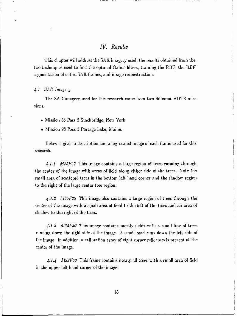
4.1.1 M85Fo27 This image contains a large region of trees running through
the center of the image with areas of field along either side of the trees. Note the
small area of scattered trees in the bottom left hand corner and the shadow region
to the right of the large center tree region.
4.1.2 AIS5Fr,28 This image also contains a large region of trees through the
center of the image with a smiall area of field to the left of the trces and an area of
shadow to the right of the trees.
4.1.3 M85F30 This image contains mostly fields with a small line of trees
running down the right side of the image. A small road runs down the left side of
the image. In addition. a calibration array of eight corner reflectors is present at the
center of the image.
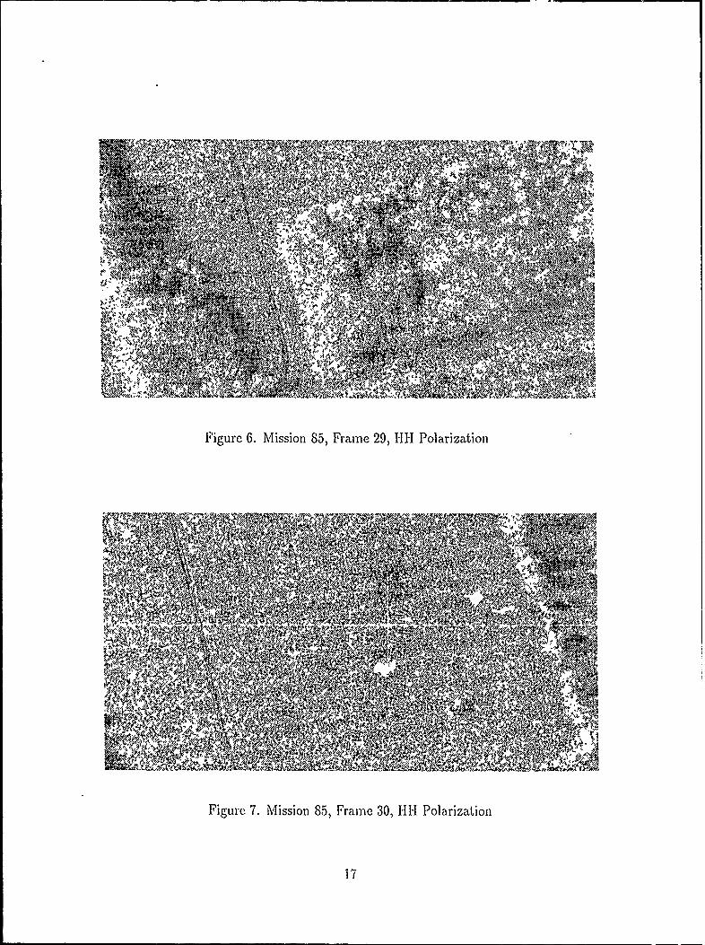
4.1.4 M98F07 This frame contains nearly all trees with a small arca of field
in the upper left hand corner of the image.
15
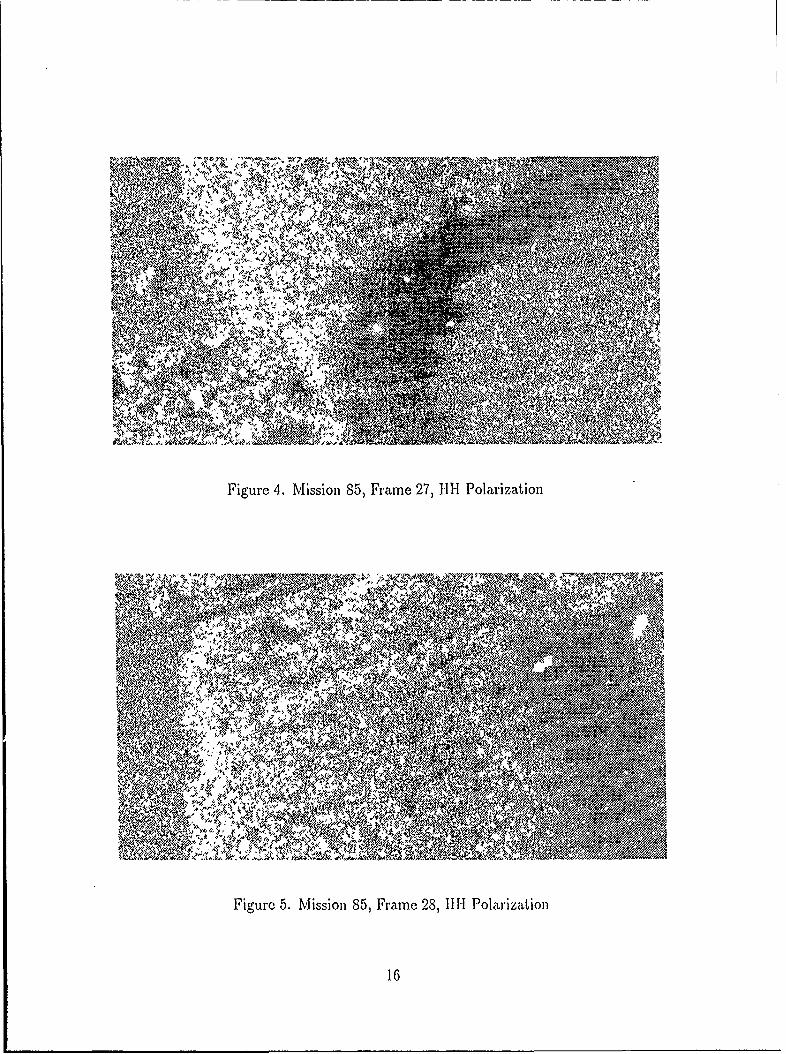
Figure 4. Mission 85, Frame 27, 111-1 Polarization
ON -,N ~
Figure 5. Mission 85, Frame 28, 111-1 Polarization
16
'41~
Figure 6. Mission 85, Frame 29, HI- Polarization
Figure 7. Mlission 85, Frame 30, 1-11! Polarization
17
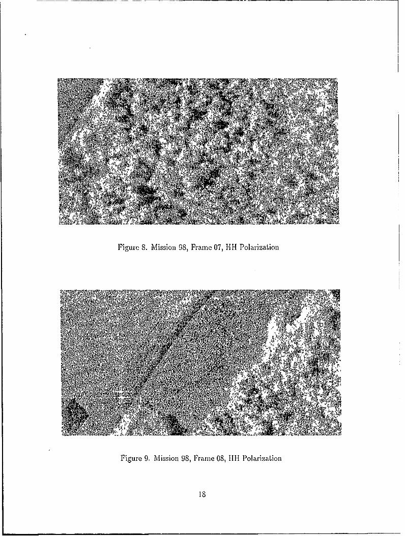
Figure 8. Mission 98, Frame 07, H11 Polarization
Figure 9. Mission 98, Framne 08, 111-1 Polarization
i8
~~& AR. AA
VS
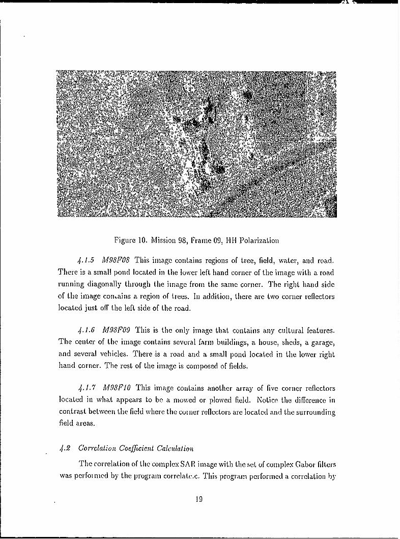
Figure 10. Mission 98, Frame 09, HH Polarization
4.1.5 M98F08 This image contains regions of tree, field, water, and road.There is a small pond located in the lower left hand corner of the image with a roadrunning diagonally through the image from the same corner. The right hand sideof the image contains a region of trees. In addition, there are two corner reflectorslocated just off the left side of the road.
4.1.6 M.98F09 This is the only image that contains any cultural features.The center of the image contains scvcral farm buildings, a house, shcds, a garage,and several vehicles. There is a road and a small pond located in the lower righthand corner. The rest of the image is composed of fields.
4.1.7 M98F10 This image contains another array of five corner reflectorslocated in what appears to be a mowed or plowed field. Notice the difference incontrast between the field where the cot ner reflectors are located and the surrounding
field areas.
4.2 Corrclation Coefficicnt Calculation
The correlation of the complex SAR image with the set of complex Gabor filters
was perfolined by the program correlatc.c. This program performed a correlation by
19
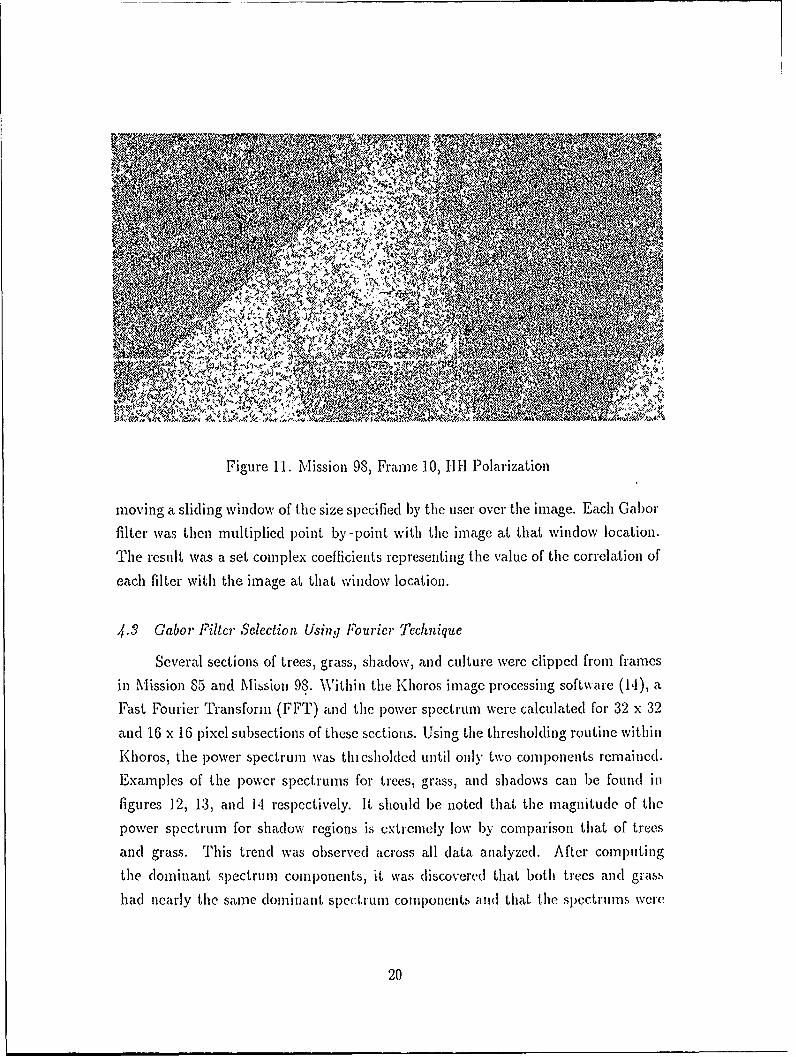
Figure 11. Mission 98, Frame 10, 111 Polaization
moving a sliding wvindow of the size specified ly the user over the image. Each Gaborfilter was then multiplied point-by-point with the image at that window location.The result was a set complex coefficients representing the value of the correlation of
each filter with the image at that v%'ndlow location.
,3 Gabor Filter Selection Using Fourier Technique
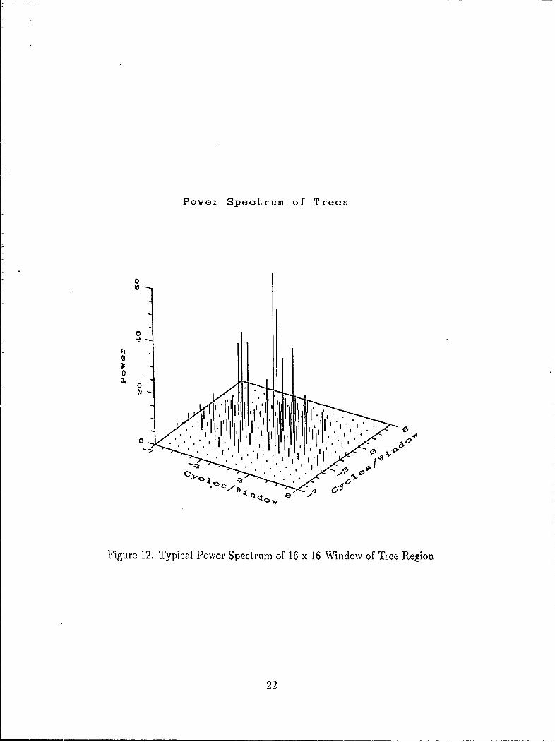
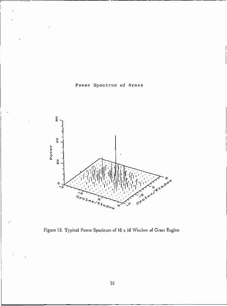
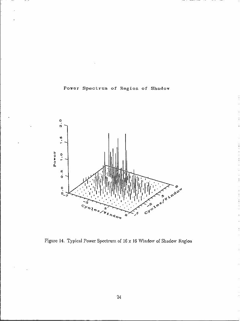
Several sections of trees, grass, shadow, and culture wvere clippIcd fromn framesin Mission 85 and Mission 98. Within the Khoros image processing software (14), aFast Fourier Transform (FFT) and the power spectrum were calculated for 32 x 32and 16 x 16 pixcl subsections of these sections. Using the thresholding routine withinKhoros, the power spectrum was thisholded until only two components remainced.Examlepis of the )owVcr spectrums for trees, grass, and shadows can be found infigures 12, 13, and 14 reslpectively. It should be noted that the iagnitude of the
power spectrum for shadow regions is extremely low by comparisonl that of treesand grass. This trend was observed across all data analyzed. After computingthe dominant spectrum components, it was discovered that both trees and grasshad nearly the same dominat Sl)CCtrumf coml)Onents aud that the spectrums were
20
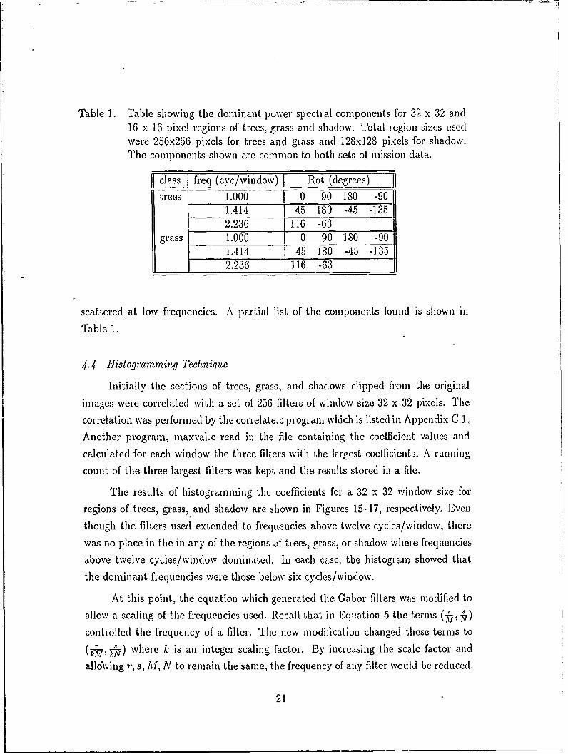
Table 1. Table showing the dominant power spectral components for 32 x 32 and16 x 16 pixel regions of trees, grass and shadow. Total region sizes usedwere 256x256 pixels for trees and grass and 128x128 pixels for shadow.The components shown are common to both sets of mission data.
class q (cyc/window) Rot (degrees) JJtrees 1.000 0 90 180 -90
1.414 45 180 -45 -1352.236 116 -63
grass 1.000 1 0 90 180 -901.414 45 180 -45 -1352.236 116 -63
scattered at low frequencies. A partial list of the components found is shown in
Table 1.
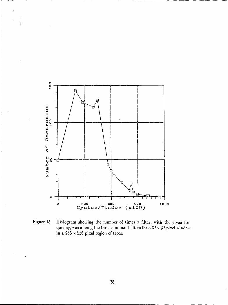
4.4 Histogramming Technique
Initially the sections of trees, grass, and shadows clipped from the originalimages were correlated with a set of 256 filters of window size 32 x 32 pixels. Thecorrelation was performed by the correlate.c program which is listed in Appendix C.1.
Another program, maxval.c read in the file containing the coefficient values and
calculated for each window the three filters with the largest coefficients. A running
count of the three largest filters was kept and the results stored in a file.
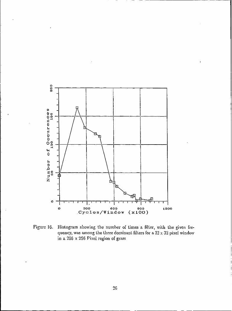
The results of histogramming the coefficients for a 32 x 32 window size for
regions of trees, grass, and shadow are shown in Figures 15-17, respectively, Even
though the filters used extended to frequencies above twelve cycles/window, there
was no place in the in any of the regions of tiees, grass, or shadow where frequencies
above twelve cycles/window dominated. In each case, the histogram showed that
the dominant frequencies were those below six cycles/window.
At this point, the equation which generated the Gabor filters was modified to
allow a scaling of the frequencies used. Recall that in Equation 5 the terms (P N)
controlled the frequency of a filter. The new modification changed these terms to(hrl',k) where k is an integer scaling factor. By increa.sing the scalc factor and
allowing r,.S, III, N to remain the same, the frequency of any filter would be reduced.
21
Power Spectrum of Trees
0
0
0
Figure 12. Typical Power Spectrum of 16 x 16 Window of Tree Region
22
Power Spectrum of Grass
0
0
0
0 0
''it* 4
. I I i
O .. ,. ° " "
Figure 13. Typical Power Spectrum of 16 x 16 Window of Grass Region
23
Power Spectrum of Region of Shadow
0
In
V0
0
00
Figure 14. Typical Power. Spectrumn of 16 x 16 Winidow of Shadow Regioni
24I
0
0tH
0z!
o Ii__ _ ' _ __ _ _ _ _
- __ ___ _ __ _ _ . .. . ._
O~u
0 T T
- I
o 300 G0t g00 1200
Cycles/findow (xlOO)
Figure 15. 1istogram showing, the number of times a filter, with the given fre-quency, was among the three dominant filters for a 32 x 32 pixel windowin a 256 x 256 pixel region of trecs.
25
0
* I.
I I0E
C)
0~
o o
0 - -0
0 300 600 000 1200*Cycles/Window (xlOO)
Figure 16. Histogram showing the number of timies a filter, with the given fre-quency, was amiong the three dominant filters for a 32 x .32 pixel windlowin a 2.56 x 256 Pixel region of grass
26
0 _ _ _ _ __ _ _ __ _ _ _
U)o
Oo
0
00 30 _00 9010
Cycles/Wfindow (xlOO)
Figure 17. Histogram Showing the number of timies a filter, with the given fre-quency, was among the three dominant filters for a 32 x 32 pixel windowin a 128 x 128 p~ixel region of shadow
27
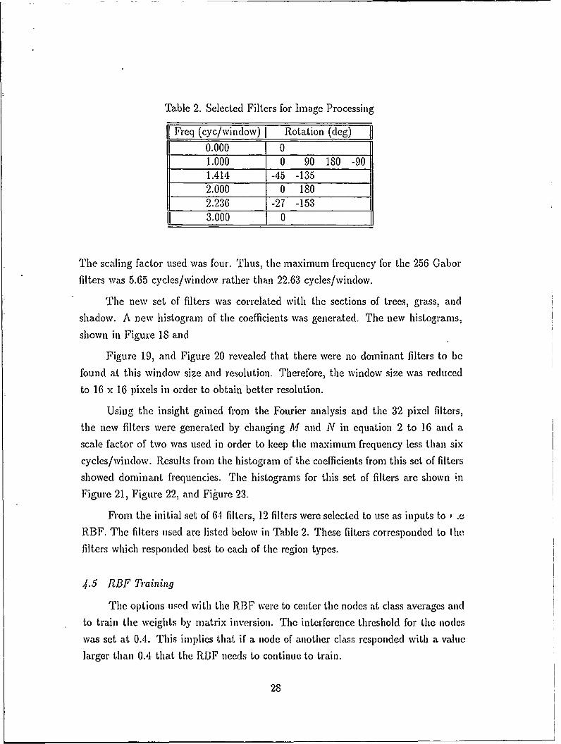
Table 2. Selected Filters for Image Processing
I[ Freq (cyc/window) Rotation (deg)0.000 01.000 0 90 180 -901.414 -45 -1352.000 0 1802.236 -27 -1533.OOO J 0
The scaling factor used was four. Thus, the maximum frequency for the 256 Gaborfilters was 5.65 cycles/window rather than 22.63 cycles/window.
The new set of filters was correlated with the sections of trees, grass, and
shadow. A new histogram of the coefficients was generated. The new histograms,
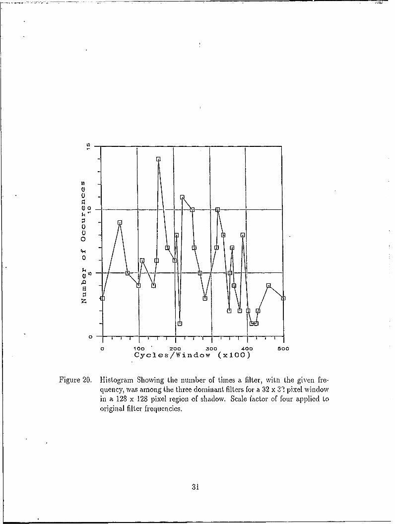
shown in Figure IS and
Figure 19, and Figure 20 revealed that there were no dominant filters to be
found at this window size and resolution. Therefore, the window size was reduced
to 16 x 16 pixels in order to obtain better resolution.
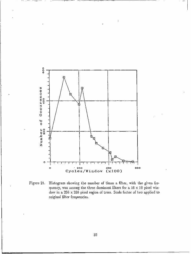
Using the insight gained from the Fourier analysis and the 32 pixel filters,
the new filters were generated by changing Al and N in equation 2 to 16 and a
scale factor of two was used in order to keep the maximum frequency less than six
cycles/window. Results from the histogram of the coefficients from this set of filters
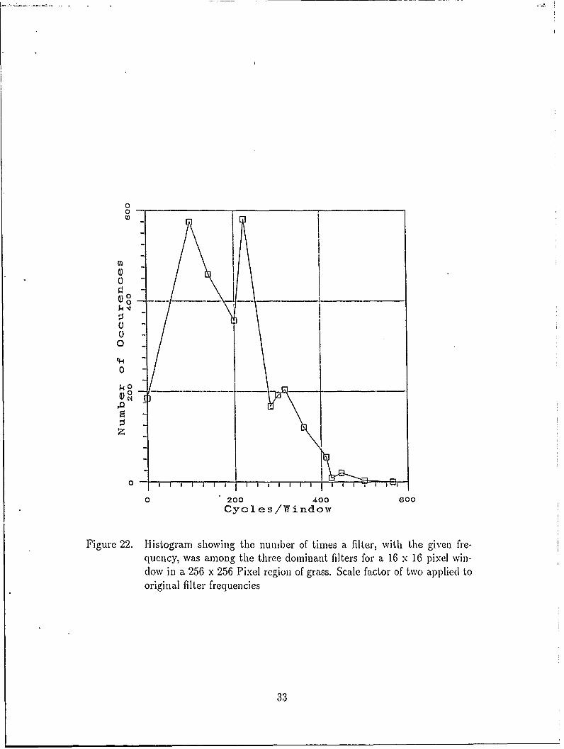
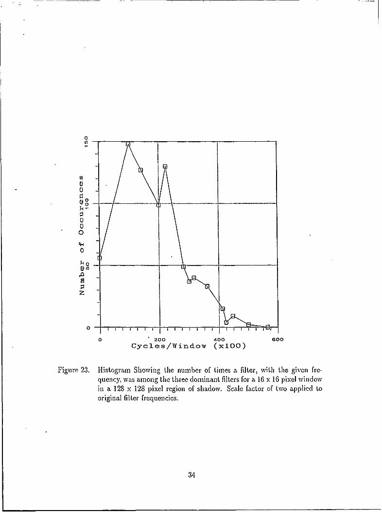
showed dominant frequencies. The histograms for this set of filters are shown in
Figure 21, Figure 22, and Figure 23.
From the initial set of 6t filters, 12 filters were selected to use as inputs to IeRBF. The filters used are listed below in Table 2. These filters corresponded to the
filters which responded best to each of the region types.
4.5 RBF Taining
The options used with the RBF were to center the nodes at class averages and
to train the weights by matrix inversion. The interference threshold for the nodes
was set at 0.4. This implies that if a node of another class responded with a value
larger than 0.4 that the RBF needs to continue to train.
28
0 0
0
0Oo-__4____
0
LI
Cycls/Widow(xlOO)
Figure 1S. H-istogrami shiowing, the number of times a filter. with the given fre.qucnicy~ was among the three dominiaut filters for a :32 x .32 pixel wini-dow iii a 2A6 x 2.56 pixel regioni of trees. Scale factor of four applied toorigial filter frequencies.
29)
0.
=: 0
00
Oo-___
0)
0 200 400 G00
Cycles/Window (xlOO)
Figure 19. H-istogramn showing the number of times a filter, with the given fre-qluency, was amiong the three doiniant filters for a 32 x 32 pixel win-dow in a 256 x 256 Pixel region of grass. Scale factor of four applied tooriginal filter frequencies
30
0
o
0
o
I I _ _ _ _
0 100 200 300 400 500Cycles/Window (xlOO)
Figure 20. Histogram Showing the number of times a filter, withi the given fre-quency, was among the three dominant filters for a 32 x 32 pixel windowin a 128 x 128 pixel region of shadow. Scale factor of four applied to
original filter frequencies.
31
00
0o0o
o
P0 -0
,0
0 200 400 600
Cycles/Window (x1OO)
Figure 21. H-istogram showig the niumber of times a filter, with the giveni fre-quency, was amonig the three dominiant filters for a 16 x 16 p~ixel wi-dow ini a 256 x 256 p~ixel region of trees. Scale factor of two applied tooriginal filter frequenicies.
32
0
0
0
0
o 200 400 600
Cycles/Window
Figure 22. H-istogramr showing the number of times a filter, with the given fre-quency, was amnong the three domninant filters for a 16 x 16 p)ixel win-dow in a 256 x 256 Pixel region of grass. Scale factor of two applied tooriginal filter frequencies
33
0
"* I
C) I0
o i_ _ _ _ _ _
o !
0
0 -
0 200 400 600
Cycles/Window (xlOO)
Figure 23. Histogram Showing the iiumber of times a filter, with the given frc-quency, was among the three dominant filters for a 16 x 16 pixel windowin a 128 x 128 pixel region of shadow. Scale factor of two applied to
original filter frequencies.
34
The RBF was trained using cross-validation technique. In other words, initially
data from Mission 85 was used as training data while Mission 98 data was used as
test data. Next, the process was reversed and Mission 98 data was used for training
and Mission 85 data was used for testing. In each case, 50 vectors for every class
of data were used for both training and testing. The training and testing vectors
were sampled from a large number of vectors available. Specifically, there werc 2018
vectors for trees and grass regions and 496 vectors for shadow regions. The program
pickval.c allowed sampling of these data files starting at any location and sampling at
any integer interval. The training and test data were statistically normalized using
the program norm.c. The normalization process was to aid the RBF in generalizing.
4.6 Training Results
The RBF was trained and tested 50 times using various combinations of train-
ing and test data. In every case, the RBF was able to achieve 97 to 100 percent
accuracy classifying the training data correctly. However, depending upon the test
data presented, the classification accuracy of the test data was as high as 93 per-
cent and as low as 65 percent. Average accuracy for test data classification was
81 percent.
Jj.7 Segmentation Results
The first test image was Mission 98, Pass 3, Frame 07 (M98P3F07) shown ill
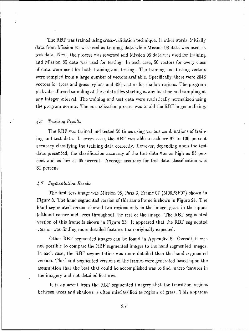
Figure 8. The hand segmented version of this same frame is shown in Figure 241. The
hand segmented version showed two regions only in the image, grass in the upper
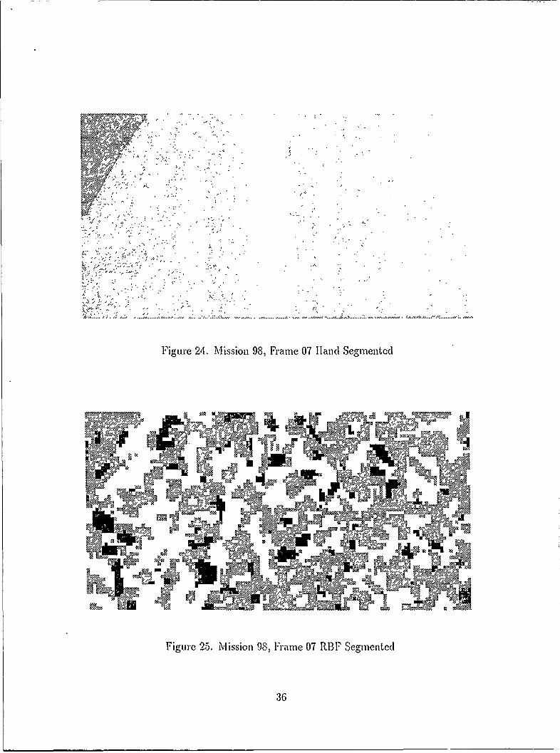
lefthand corner and trees throughout fihe rest of the image. The RBF segmented
version of this frame is shown in Figure 25. It appeared that the RBF segmented
version was finding more detailed features than originally expected.
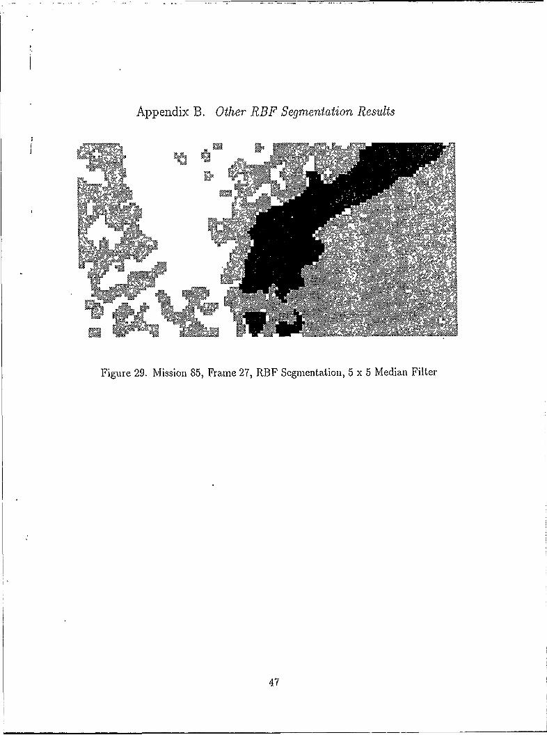
Other RBF segmented images call be found in Appendix B. Overall, it was
not possible to compare the RBF s-gmented images to the hand segmented images.
In each case, the RBF segmenation was more detailed than the hand segmented
version. The hand segmented versions of the frames were generated based upon the
assumption that the best that could be accomplished was to find macro features in
the imagery and not detailed features.
It is apparent from the RBF segmented imagery that the transition regions
between trees and shadows is often misclassified as regions of grass. This apparent
.35
I iguic 24. Mission 98, Framec 07 Hand Segmented
Figure 25. Mlission 98, Frame 07 RBF Segmiented
36
weakness could be explained by the fact that all of the filters used to process the
SAR imagery were of low fiequency. The lack of high frequency information makes
it difficult to find edges.
It appeared that the discrepancy in the accuracy of the ability of the RBF to
classify the test data correctly could be explained by the fact that the regions of
trees in the Mission 98 data contained areas of shadow. In addition, after examining
the previous work of L'Homime, it was discovered that the data from Mission 98
contained higher radar return va!ues for areas of trees and grass than did Mission
85. This could also be a source of error.
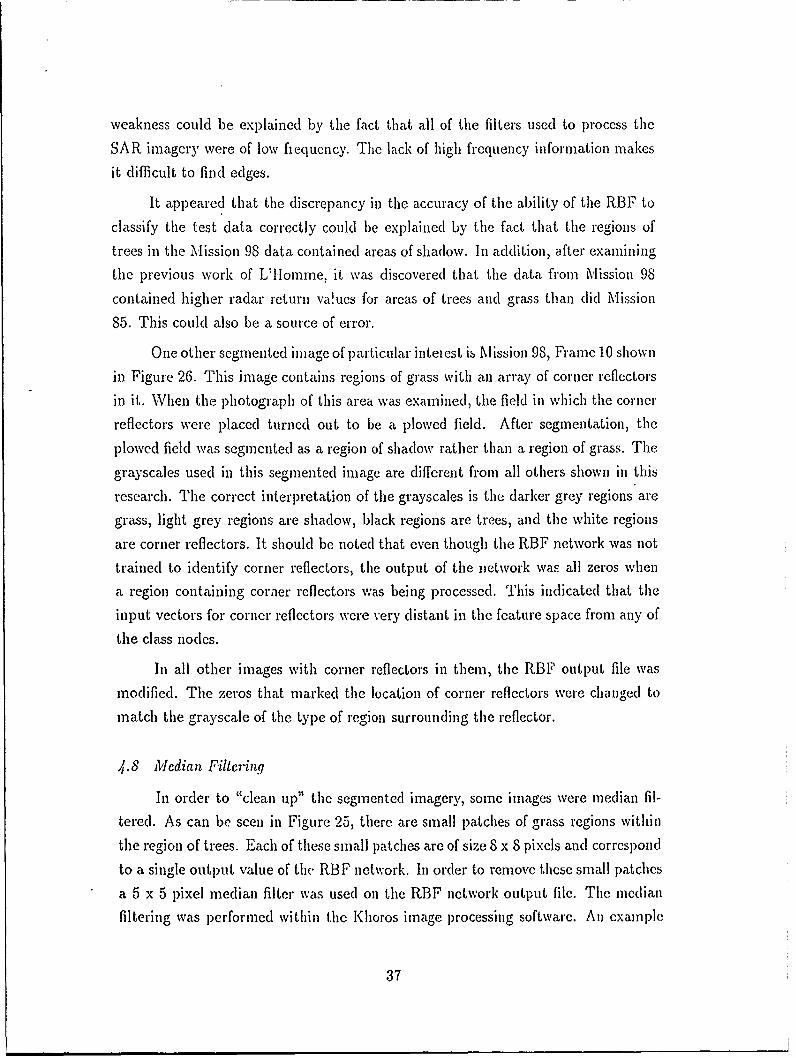
One other segmented image of particular inteiest is Mission 98, Frame 10 shown
in Figure 26. This image contains regions of grass with an. array of corner reflectors
in it. When the photograph of this area was examined, the field in which the corner
reflectors were placed turned out to be a plowed field. After segmentation, the
plowed field was segmented as a region of shadow rather than a region of grass. The
grayscales used in this segmented image are different from all others shown in this
research. The correct interpretation of the grayscales is the darker grey regions are
grass, light grey regions are shadow, black regions are trees, and the white regions
are corner reflectors. It should be noted that even though the RBF network was not
trained to identify corner reflectors, the output of the network was all zeros when
a region containing corner reflectors was being processed. This indicated that the
input vectors for corner reflectors were very distant in the feature space from any of
the class nodes.
In all other images with corner reflectors in them, the RBF output file was
modified. The zeros that marked the location of corner reflectors were changed to
match the grayscale of the type of region surrounding the reflector.
4.8 Median Filtering
In order to "clean up" the segmented imagery, some images were median fil-
tered. As can be seen in Figure 25, there are small patches of grass regions within
the region of trees. Each of these small l)atches are of size 8 x 8 pixels and correspond
to a single output value of the RBF network. In order to remove these small patches
a 5 x 5 pixel median filter was used on the RBF network output file. The median
filtering was performed within the Khoros image pmrocessing software. Ai example
37
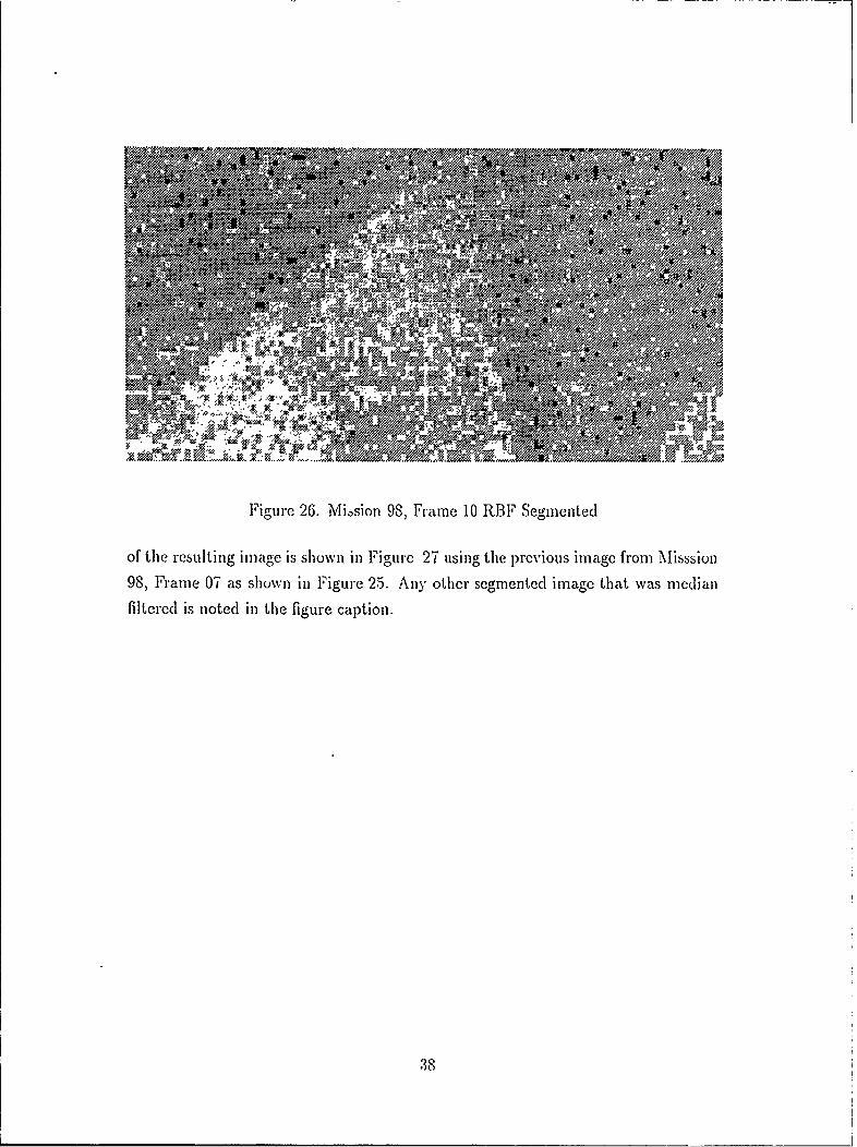
Figure 26. Miosion 98, Frame 10 RBF Segmented
of the resulting image is shown in Figure 27 using the previous image from Misssion98, Frame 07 as shown in Figure 25. Any other segmented image that was median
filtered is noted in the figure caption.
38
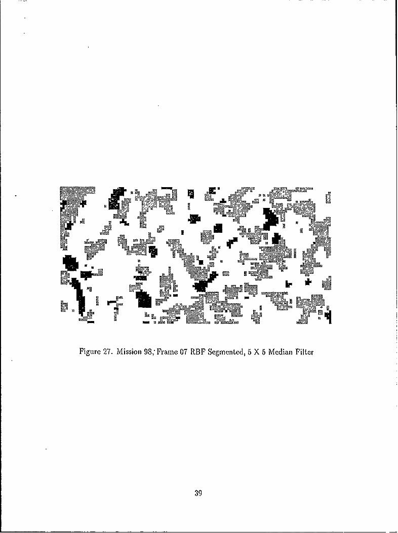
Figure 27. Mission 98," Frame 07 RBF Segmented, 5 X 5 Median Filter
39
V. Conclusions and Recommendations
5. 1 Introduction
This research investigated the use of Gabor filters to segment high resolution
SAR imagery. The aim was to find a set of Gabor filters which could be used to
locate regions of trees, grass, and shaduw using the complex representation of the
SAR image. In particular, the following questions were answered during this work.
* Can the Fourier technique suggested by Bovik help to select the correct com-
bination of filters to use for segmenting regions of trees, grass, and shadow?
* Can Histogramming techniques perform the same task?
" Can a RBF network learn the --orrect combination of filters to generalize to a
full SAR image?
The Fourier technique showed that naturally occurring regions, in these SAIR.
images, responded best to frequencies below 4 cycles per window (16 and 32 pixels).
In addition, this analysis also showed that the phase of naturally occurring regions
is widely scattered. In general, however, this technique did not work to isolate the
correct Gabor filters to use. The cases which Bovik used were images with only one
or two dominant textures in them. It appears that this technique is not useful for
cases involving regions with more than two easily seen textures in them.
Histogramining was able to isolatc a set of Gabor filters to use once the window
size was reduced to 16 pixel's. The Gabor filters isolated were all of low frequency
(less than 4 cycles per window). Essentially, this technique found the bandpasses of
frequencies that regions of trees, grass, and shadows responded to best.
The RBF network achieved testing accuracies as high as 93 percent and aver-
aged 81 percent correct. However, due to the problem of normalization, the R13F
network was not able to generalize well to entire images.
5.2 Further Rcscarch
Below are listed suggestions for further research.
410
* To allow consistent scaling across images, use another type of normalization.
One suggested method would be a local normalization within each window.
* Find another technique for selection of the Gabor filters.
* Continue to use overlapping windows of other sizes such as 8 by 8 or 4 by 4.
The overlapping windows appear to be able to find greater detail in the SAR
imagery than do independent windows.
* Continue to use the RBF network. If the normalization problem is solved, the
RBF should provide good segmentation across images.
e Try adding other polarizations to the Gabor processing as features for the 1tBF
network.
41
Appendix A. The Gabor Representation
The only difficulty in working with the Gabor functions is that while the func-tions do form a complete basis set onto which to map an image, they are not or-thogonal. This implies that when attempting to find the set of coefficients that
appropriately map the image onto the Gabor functions, the inner product terms
[g,(x, y)- g(.r, y]) between filters are non-zero. Recent literature by J)augman (3)has shown that the efficient way to find the Gabor representation of an image isthrough use of an artificial neural net (ANN). The ANN used contained three layers.The first layer was made up of a set of fixed weights assigned as the value of the
Gabor functions. The second layers contains a set of adjustable weights that are usedto multiply the output of the neurons in the first layer. The third layer is again madeup of a set of fixed weights assigned as the value of the Gabor functions. The layer ofadjustable weights, upon completion of learning, were the complex coefficients thatrepresented the projection of the image onto the Gabor functions. These coefficients
are the optimal coefficients in the sense of the minimal mean-squarced-error. A moredetailed proof of this mean- squared-error minimization is given below.
Computing of the Gabor coefficients will be accomplished by implementing theANN suggested by Daugian (3) and shown below in Figure 28.
Using the Gabor functions as the set of basis functions to represent an image
poses a difficult problem. Although the Gabor functions com)rise a complete set offunctions, that is, they can represent any function, they are not orthogonal. Thismeans that the solution for the coefficients. a,,, cannot be computed by the simpleintegration of the original image with the complex conjugate of the ith basis function
,(., y). Starting from an image I(x, y) represented as a sum of projection coefficientstimes a set of basis functions, each image pixel is computed as follows:
I(X' Y) = aiqS(x, y)
":1
a: I(X, k(X, y) dXdy - ,I(xy)(xy)(x,) d
0 j=1 j-riy)
412
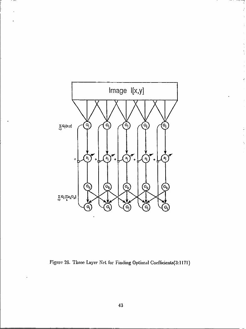
Image I[x,y]
7ZG1ifx.yI - G i G
Y-Gi [-a kGkIk
Figurc 28. Three Layer Net for Finding Optimnal Coefficienits(3:1171)
4.3
where: I(x, y) - original image
H(x, y) - reconstructed image
a,,- expansion coefficients
0,,(x, y) - basis function
Now had the original basis functions been orthogonal, all the terms in the
solution for the a, coefficient containing the form 0*(x, y)q5 (x, y) would be equal to
zero. But, because the set of Gabor functions is not orthogonal and because we only
wish to use a subset of the Gabor functions, the best that can be accomplished is
an optimal fit. The particular optimization criterion used by Daugman is that of
minimizing the squared norm of the difference voctor:
E =11 I(x,y) - H(x,y) 12
where: H(x,y) = Et, ajoi[x,y] and
Oi[x, y] are the elementary Gabor functions.
In order to minimize the norm, the partial derivative with respect to each of
the coefficients must equal zero. Substituting for I and computing the derivative
yields:
ak= -2 Z[I(x, y)o(x, y)] + 2 [E akqk(X, y)] = 0ai *, x,y k=1
The result is a set of n equations of the form:
E I(x, y)Oi(x, y) = Z[6'-.(x, y)(E akq~k(X, Y))]xy Xy k=i
Daugman points out that these equations could be solved with matrix manip-
Illation, but the number of calculations necessary would be immense. He also points
out that the error surfce *.s quadratic in each a,. Since neural nets can be used to
minimize an error functin, he proposes his net as a solution to this problem.
44
The net sets up the error surface as the squared norm of the difference betweenthe original image and the current approximation. He then uses gradient descent tofind the minimum of the error surface. Examining Figure 28, the first layer of the
net yields the product of each of the elementary Gabor functions ,[x,y] with theoriginal image (i.e. the Gabored image). The third layer of the net yields the inner
product of each elementary function with the linear combination of all the functions(i.e. the reconstruction from the Gabor coefficients). Finally, the second laycr is the
layer used to calculate the coefficients. Initially, the second layer is set equal to the
product of each Gabor function with the image. Then, by using gradient descent, thecoefficients of the second layer are adju-ted according to the following relationship:
ai = ai + Ai
Wherc: Ai = Zx,,(J, Vy[x, ]) - ZI7d(EkL1 akqAXy])
Or in other words, the difference between the product of the Gabor function withthe original image and the Gabor function with the reconstructed image. The net is
allowed to iterate until the adjustments, Aj, equal zero.
Put simply, the first layer computes the correlation of the image with the basisset. These coefficients are then used to reconstruc a new image j[a, k(X, y)]. The
third layer correlates the reconstructed inage with the basis set. The result of tile
third layer correlation is compared to the correlation from the first layer and theadjustment to the coefficients is made. When the adjustment to each coefficient,
A,, is zero, the iteration process is terminated and the coefficients are read fromthe weights of the second layer. Overall, the function of the net is to calculate the
amount of correction necessary to account for the non-zero inner products of each ofthe functions with all other functions as a result of the non-orthogonality of Gabo
functions.T ihe initial implementation of the Gabor filters was as given in Daugman. The
Gaussian envelope was supported on a 32 X 32 window with the 1/c point set at
±9 pixels and tapered to a value of 0.05 at the windows edge where the value was
truncated to zero. These 32 X 32 windows were moved across the image in steps of
one-half tile wi~low size. So for the case of a 32 X 32 window the step size was 16
pixels.
45
Implementation of the network was done, but it failed to converge as described.
Several modifications were made to the network and it still would not converge. Tle
initial test of the Lenna image resulted in the network diverging rapidly while trying
to find the optimal coefficients. Tests with other images did exactly the same thing.
It was later learned from a graduate student from University of Tennessee (13)
that he had experienced the same problem while trying to implement Daugman's
network. His fix had been to use only real images and the real (cosine) portion of
the Gabor filters. In addition, his first estimate of the a, coefficients had been the
largest pixel value in the window of interest.
46
Appendix B. Other RBF Segmentation Results
Figure 29. Mission 85, Frame 27, RBF Segmentation, 5 x 5 Median Filter
47
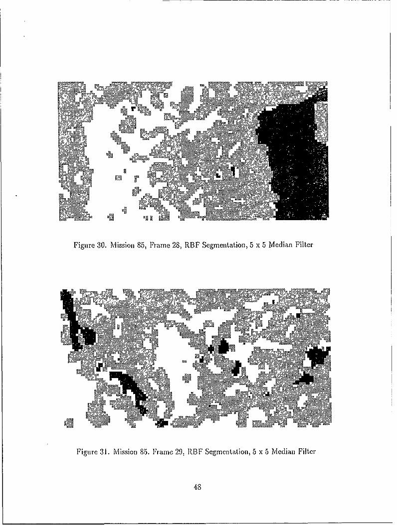
Figure 30. Mission 85, Frame 28, RBF Segmentation, 5 x 5 Median Filter
Figure 31. Mission 85. Frame 29, R13FSegmentation, 5 x 5 M'vedian Filter
48
A. 2". m~
g Mno< - 6%7 w
- MRl,
~~~Figure 33. Mission 98, Fame 08, RBF Segmentation einFle
49~
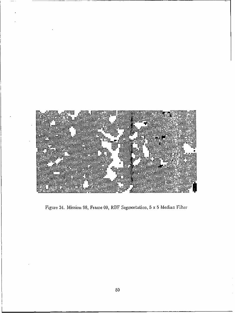
Figure 34. Mission 98, Frame 09, RBF Segmentation, 5 x 5 Median Filter
50
Appendix C. Program Listings
C. I correclate.
/* -------------------------------------------------------/* Program: correlate.c
1* Author: Michael Hazlett *1* Purpose: Correlates an image with the given set of filters. */* ------------------------------------------------------- *
#include <stdio .h>#include <math.h>
#define TRUE 1#define FALSE 0#define SQR(a) ((a)*(a))#define SQR2(a) ((double) ((a)*(a)))
void maino
float **matrixQ, *vectoro;void fourno, free.vectoro, free-matrixO%;
FILE *fp, *gp, *hp;int numdim =2, sign -'1, wsize, isize[2], sizeE2];int hwin, vwin, nwin, win;int xy, xsize, ysize, 1, xr, xi;int ireal, nfilt;mnt winr, wini, winnum, filt;int row, col;int h, i, j, k, x, y, 1M, N;char gfile[60], cfile[6O], if ile[60] , cfile2[60], stype[2];char itype[2] , dtype[2] , dname[SO) , rmode[3], yn[2] , cnaine[S];float **a!, **image, **gabor, **temp, *norms;double minval = 0.0000100;
strcpy(rmode, "r");
51
printf("\nName of image filescanf("Y/s", ifile);
printf("\nls the image Rleal or [Clomplexscanf("s", itype);
if(!(strcmp(itype, "R")) I I !(strcmp(itype, "r"))) {printf("\nAre the numbers [F]loat or [I]nteger 11)scanf("s", dtype);
}else {
printf("\nIs the file stored in [A]SCII or [I]nternal format?:t");
scanf("/s", stype);
if(!(strcmp(stype, "I")) II !(strcmp(itype, "i"))) {strcpy(rmode, "rb");
}}
printf("\nSixe of image vertically (pixels)scanf("%d", &isize[O]);
printf("\nSize of image horizontally (pixels)scanf("Xd", &isize[1]);
printf("\nWindow size of Gabor functions (pixels)scanf("/d", &wsize);
printf("\nNumber of filters : );
scanf("Y,d", &nfilt);
printf("\nDirectory where filter files atscanf(",s", dname);
printf("\nName of coefficient file to createscanf(",s", cfile);
/* ------------------------------------ ,/I* Initialize arrays and other variables *I/* /-----------------------------
M = wsize / 2;xsize = isize[l] + M+1;ysize = isize[O] + M+1;
52
hwin = isize~l] / M;vwin = isize[O] / 1M;nwin = hwin * vwin;
imaie = matrix~i, ysize, 1, 2*xsize);al = matrix~l, nfilt, 1, 2*nwin);gabor =matrix(1, wsize, 1, 2*wsize);norms = vector~i, nwin);
/* -----------------/* Open the image file */* -----------------if ((fp = fopen~ifile, "r"))=NULL)
printf("Error opening file %/s", if ile);exit(1);
/* ------------------------ *1* Read in the image file data */* ------------------------ *
/* Data stored is only real numbers *
if(!(strcmp(itype, "r"l)) 11 !(strcmp(itype, "R"))
/* Real numbers, data values are integers */
if(!(strcmp(dtype, "ill)) 11 !(strcmp(dtype, "I"))){
for(i=1; i <= ysize; i++) {for(j=1; j <= xsize; j++){
xr =2*j-l;xi =xr+1;if(i > M4/2 && i <= ysize-M/2-1 &&
j > 1M/2 && j <= xsize-M/2-1){
fscanf(fp, I/d\ntl, &ireal);image [ii Exr] = (f loat)ireal;image[i] [xi] 0.0;
else{image[i] [xr] = 0.0;image[i] [xi] = 0.0;
5.3
1* Real numbers, data values are f loat *
else{
for(i=1; i <= ysize; i++){for(ji; j <= xsize; j++){
xr = 2*j-l;
xi = xr + 1;if(i > M/2 &&i <= ysize-M/2-1 U&
j > M/2 &&j <= xsize-M/2-1) ffscanf (fp, "Y/f\n", &image [i] [xr));image[i] [xi] = 0.0;
else{image[i]I~xr] = 0.0;
image~i][xi] = 0.0;
/* Data is stored as complex pairs *
else f
1* Complex pairs are stored in ASCII format *
if(!(strcmp(stype, "A'")) 11 !(strcmp(stype, "a"))){
for(i=1; i <= ysize; i++) ffor(j=4; j <= xsize; j++){
xr = 2*j-l;xi = xr + 1;if(i > M4/2 && i <= ysize-M/2-1 &&
j > M/2 && j <= xsize-M12-1) {fscanf (fp, '7,f Y/f\n", &image [ii [xr],
&image [il [xi]);
else{image [-]I xr] = 0. 0;
541
image~i] [xi] =0.0;
1* Complex pairs are stored in INTERNAL format *
else {
temp =matrix(1, isize[O], 1, 2*isize[Il);
for(i=1; i <= isize[0]; i++) {fread(temp[i], sizeof(float), 2*isize[1], fp);
for(i=1; i <= ysize; i++){for(j=i; j <= xsize; j++){
xr =2*j-1;xi = xr + 1;if(i > M1/2 && i <= ysize-M/2-1 &&
j > 1M/2 && j <= xsize-M/2-1){k =2*(j-M/2) -1;
1 =k + 1;image [i] [xr] temp [i-M/2] Ek];image [i] [xi] temp ti-M/2] El];
else{image[illxr] 0.0;image~i] [xi] 0.0;
free..matrix(temp, 1, isize[0], 1, 2*isize[1]);
fclose(fp);
/*-----------------------*/* Zero out the coefficients */*-----------------------for(i=1; i <= nwin; i++) f
55
for(j=1; j <= nfilt; j++){al[j][2*i-1] = 0.0;al[j][2*i] = 0.0;
/* --------------------------------- */* Loop through all of the Gabor filters */*------------------------------------*for(i=1; i <= nfilt; i++){
sprintf (gf ile, "/Xs~s%03d", dnaxne, "gabor", i);
if ((gp = fopen(gfile, "r"))=NULL){printf("Error opening file %/s", gfile);exit(1);
printf Q'\nGabor filter #Yd", i);
/* -------------------- */* Read in the Gabor file */* -------------------- *
for(j=1; j <= wsize; j++){for(k=1; k <= wsize; k++){
xr =2*k-1;xi = xr + 1;fscanf(gp, "Y/f Yf\n", &gabor~j] Exr], &gabor~j] [xi]);
I
fclose(gp);
/* -------------- :---------------------------------------1* Multiply the Gabor and Image point by point for each window */* ----------------------------------------------------------
for(j=1; j <= vwin; j++) {
for(k=1; k <= hwin; k++){
win =2*((j-i)*hwin +k)1
for(y=1; y <= wsize; y++) j
row = (j-l)*(wsize/2)+y;
56
for(x1l; x <= wsize; x++){
col = (2*(k-l)*(wsize/2))+2*x-1;
ai[i] [win] += image [row] [col] * gabor[y] [2*x-1]
image [row] [col+l] * -gabor~y] [2*x];al~i] [win+1] += image[row] [col+i] * gabor~y] [2*x-1]
+ image [row] [cal] * -gabDor[y] [2*x];
/* --------------------------------------- *1* Store the original coefficients in the file. */* Store by window #* then filter 1*. Normalize */* coefficients to area under Gabor. */* --------------------------------------- *
if ((p = fopen(cfile, "Iw"))==NULL) {printf ("Error opening file Ys", cf ile);exit~l);
I
fprintf(hp, "%/d U/. 7d U/. Y7dd\n", Mfilt, wsize, hwin, vwin,isize [0] ,isize [1]);
for(j=1; j <= nfilt; j++){if (f abs ((double) a![j] [2*i -1]) <minval) al[j][2*i-1] = 0.0;if (f abs ((double) al(j] [2*i]) <minval) al[j3[2*i] = 0.0;
fpitIp % .', enij lj(*-3 lj[-i)
fprintf(hp, "\n");
fclose(hp);
printf ('\nFinished computing al coefficients\n");
.57
C.2 rebuild.c
/* -- - - - - - - - -- - - - - - - - - -- - - - - - - - -
/* Program rebuild.c *//* */
/* Author: Michael Hazlett *//* Purpose: Creates an image from a file containing *//* coefficient values *//* ----------------------------------------------------- *
#include <stdio.h>#include <math.h>
void mainO
float **matrixo;int *ivectorQ;
FILE *fp, *gp;int wsize, isize[2], xsize, ysize, win, fl, f2;int hwin, vwin, nwin, xpos, ypos;int nfilt, xstart, ystart, w, *filt, f;int i, j, k, x, y;char gfile[60], cfile[32], ifile[32], gname[50], yn[2];char dname [30];float **gabor, **image, **ai;
printf("Name of coefficient file : ');scanf("/,s", cfile);
printf("\nName of image file to create :scanf("',s", ifile);
printf("\nDirectory where Gabor files at :scanf("s", dname);
* -------------------- *1/* Open the coefficient file *//* --------------------------- *if((fp=fopen(cfile, "r") )==NULL) {
printf("\nError opening %s\n", cfile);
58
exit (1);
1* Read in reconstruction info */*-------------------------*f scanf (f P, "'/d 'Ad 7.d 7.d 7,d Y.d", &nf ilt, &wsize, &hwin, &vwin,
&isize [0], &isizel]~);
/* --------------------------------- */* Initialize arrays and other variables */* ---------------------------------nwin = hwin * vwin;ysize =isize[0]+wsize/2+1;xsize = 2*(isize[l]+wsize/2+1);
filt =ivector(l, nfilt);
image = matrix(l, ysize, 1, xsize);gabor =matrix(1, wsize, 1, 2*wsize);
ai = matrix(1, nfilt, 1, 2*nwin);
sprintf (gnane, "YsYls", dname, Ilgaborl);
/* ------------------ */* Zero the image array */* ------------------ *for(i=1; i<= ysize; i++){
for(j=1; j<=xsize; j++){image~i[j] = 0.0;
/*-------------------------------------------/* Initialize filter selection array to all filters */*-------------------------------------------*for(i=1; i<=nfilt; i++){
filt[iJ = i
/*----------------------*/* Read in the coefficients */*----------------------*for(i=!; i <= nwin; i++){
59
for(j=1; j <= nfilt; j++){f scanf (f p, 117.d Yd Y/f '/f \n", &w, &f , &ai [j] [2*i-1],
&ai [j] [2*i])Ifscanf(fp, 11\n");
fclose(fp);
printf ("\nebuild the image from selected f ilter(s)? (yin)scanf('%/s", yn) ;
if(! (strcmp(yn, "ly")) 11 ! (strcmp(yn, "Y"))){
i =1
while(f && i <= nfilt){printf("\nFilter # (0 to stop)scanf("7d", &f);filt~i] = f
/*------------------------------------*
while(filt~ij && i <= nfilt){
f = filt~i];
sprintf(gfile, "'As03d", gnanie, f);
if ((gp =fopen(gfile, "r"))==NULL)printf ("Error opening file 7s", gf ile);exit(1);
I/* -------------------- */* Read in the Gabor file */* --------------------
for(j=1; j <= wsize; j++){for(k=!; k <= wsize; k++){
fscanf(gp, "Y/f Y/f\n", &gabor[j] [2*k-1], P-gabor[j] [2*k));
60
}}
fclose(gp);
/ * -- - - - - - - - - -- - - - - -- - - -- - - - - - - - -
/* Multiply each of the coefficient by the Gabor at each *//* location and sum the result to reconstruct the image. *//* /------------------------------------------
for(j=1; j <= vwin; j++) {
for(k=1; k <= hwin; k++) {
win = 2*((j-l)*hwin + k)-1;
for(y=1; y <= wsize; y++) {
ypos = (j-l)*(wsize/2)+y;
for(x=l; x <= wsize; x++) {
xpos = (2*(k-l)*(wsize/2))+2*x-i;
image[ypos] [xpos] += ai[f] [win] * gabor[y] [2*x-i]- ai[f] [win+1] * gabor[y] [2*x];
image[ypos] [xpos+l] += ai[f] [win+1] * gabor[y] [2*x-1]+ ai[f] [win] * gabor[y] [2*x];
}}
i++;
/* *-----------------------------------/* Write the reconstructed image array to a file *//* *-----------------------------------if((fp=fopen(ifile, "w"))==NULL) {
printf("Error opening %s\n", ifile);exit(1);
Iystart = (wsize/4) + 1;
xstart = (wsize/4) + 1;for(i=ystart; i <= ystart+isize[O]-1; i++) {
61

for(j=xstart; j <= xstart+isize[l]-1; j++){fprintf(fp, 117f Y/f\n", image [i] [2*j-1] , image[i] [2*j]);
I
fclose(fp);
62
Bibliography
1. Ayer, Kevin W. Gabor Transforms for Forward Looking InfraRed Image Seg-mentation. MS thesis, AFIT/GE/ENG/89D-1, School of Engineering, Air ForceInstitute of Technology (AU), Wright-Patterson AFB OH, December 1989.
2. Bovik, Alan Conrad and others. "Multichannel Texture Analysis Using Local-ized Spatial Filters," IEEE PAMI, 12(1) (January 1990).
3. Daughman, John G. "Complete Discrete 2-D Gabor Transforms by NeuralNetworks for Image Analysis and Compression," IEEE Trans. on Acoustics,Speech, and Signal Processing, 36(7):1169-1179 (July 1988).
4. Daugmah, John G. "Uncertainty relation for resolution in space, spatial fre-quency, and orientation optimized by two-dimensional visual cortical filters,"Journal of the Optical Society of America, (7):1160-1169 (July 1985).
5. Jones, P. Judson and Larry A. Palmer. "An Evaluation of the two-dimensionalGabor filter model of simple receptive fields in cat striate cortex," Journal ofNeurophysiology, 58(6):1233-1258 (December 1987).
6. L'Homme, Albert P. Gabor Filters and Neural Networks for Segmentation ofSynthetic Aperture Radar Imagery. MS thesis, AFIT/GE/ENG/90D-31, Schoolof Engineering, Air Force Institute of Technology (AU), Wright-Patterson AFBOH, 1990.
7. Lu, Shin-yee and others. "Texture Segmentation by Clustering of Gabor FeatureVectors," International Joint Conference on Neural Networks, Seattle, 1:683-687 (July 1991).
8. Novak, L. M. and others. "Optimal Processing of Polarimetric Synthetic Aper-ture Radar Imagery," .The Lincoln Laboratory Journal, 3(2) (1990).
9. Pierce, J. R. and J. E. Carlin. "Reading Rates and the Information Rate of aHuman Channel," Bell Systems Technical Journal, 36:497-516 (March 1957).
10. Porat, Moshe and Yehoshua Y. Zcevi. "The Generalized Gabor Scheme of inageRepresentation in Biological and Machine Vision," IEEE PAMI, 10:452-468(July 1988).
11. Priddy, Kevin L., et al. "Image Segmentation, Feature Extraction, and Clas-sification Using Neural Networks." Proceedings of the Sixth Annual AerospaceApplications of Artificial Intelligence Conference. ACM Press, 1990.
63
12. Ruck, Dennis W. Characterization of Multilaycr Perccptrons and their Appli-cation to Multiscusor A7,tomatic Target Detection. PhD dissertation, School ofEngineering, Air Force Institute of Technology (AU), Wright-Pattcrson AFBOH, 1990.
13. Sarif-Saref, flamcd. Personal Correspondance. University of Tennessee,Knoxville TN, 1991.
14. The Khoros Group. Khoros Alanual Volume I User's Manual. AlbuquerqueNM: University of New Mexico, May 1991.
15. Veronin, Christopher P., et al. "An optical image segmentor using waveletfiltering techniques as the front end of a neural network classifier." Procccdings ofthe SPIE 1991 International Symposium and Exihibition on Optical Enginccringand Photonics in Aerospace Sensing. Bellingham, WA: SPIE Press, 1991.
16. Wong, Yiu-fai. "How Gaussian Radial Basis Functions Work," IJCNAN, Seattle,H:133-137 (July 1991).
17. Zahirniak, Daniel R. Characterization of Radar Signals Using Neural Networks.MS thesis, AFIT/GE/ENG/90D, School of Engineering, Air Force Institute ofTechnology (AU), Wright-Patterson AFB OH, 1990.
18. Zahirniak, Daniel R and others. "Pattern Recognition using Radial Basis Func-tion Networks." Prepared for AIAAA Conference.
64
J
1AGENCY USE Cn~~' bh o" ) 2 RE 191777MP'T S c~
4 TITI i2D 'sJRWILF S FUNOW'6 NUWMERSGabor ementation of High Resolution Synthetic Apertur
Radar Imiagery
6. AUi 4 l A. Hlazlett, Captain, USAF
7. PERFORMING ORG3;5MZATP3,1A-I $ A1:) SSk $ V-VA~ tPAZAiAir Force Institute of Technology, WPAFB Oll 45433-6583 7E-ORT N42?i
A FIT/'G E/EING/9 1 D-23
9. SONSRIN, P.0flTO~-,r AGHIC, NA%':S) ND A~p-S~t--)10. SPONSORING tAONITORING
9. SON5OiNG~N;OriTORc AGNC(AGENJCY REPOR{T NUMLSER
11. SUPPLEMEN4TARY NOTES
12a. DtSTRIBUTI -AVAIIABIUiT STAT-MVEMT 112b DISTRIBUTION CODE'~~~rv~for public release; dis tribution unlimited
13, An'TRA T n C 'r bcsbirv~cbtigate ue vf G~bvr filterb and a raital babis function (RB!') nut."rk fur btpicudtativii of high
resolutioni (I foot by I foot) s~ynthetic apcrturc radlar (SAR) imiager%. Prucc,-,iig linuokd corrulation beL%%eenthe SAR imagery and Gabor functins Tiwo iiietluds for s..lcctin the optinal Cabor filtters arc pru-eiitcd. Tbis,rescarch uscd coniplex Gabor functions. and operated on :,ingle polarizatiuli 11l1 culilpiex data. rl 0ul ilig teselectiont of the proper Gabor filters1 Lurrelationi cucflicliijt fur each illiage %%cre- calculatedl and tued a., featuresbfor the RBF network. Pruvided arc results deriiontrAting liu%% Gabovr processbing and it RBr iiact%%ork Iprovide;image segmentation.
~ ->
Gabor Fuinctions, Image Analysis, Segmentation
17 590AuT~ ~ '-, iT0 C_ r I ~~"nr iidUnclassified lindassificd I 11
GENERAL INSTRUCTIONS FOR COMPLETING SF 298
The Report Documentation Page (RDP) is used in announcing and cataloging reports. It is important-that this information be consistent with the rest of the report, nartcularly the cover and tale piagaeinstructions for filling-in eachblock of-the form follow. It is important to stay within the lines to meet
7 optial-canningrequirements.
Block 1. Lency Use Only (Leave blank) Block 12a Distribution/Availability StatementDenotes public availability or limitations. Cite any
_Block 2. Report Date. Full publication date avalabiity tote public. Enter additional-ludingay, month, and-year, if available (eg i limitations-or specal markings in all capitals (e~g.Jan 88). Must cite atleastthe-year. NOFORN, REL, ITAR).
Block 3. -tpe of Report anc Dates CoveredDState whether report-is interim, final, etc. If DOD TSee DoDDi5230.24, 'Dlstnbution
applicable, enter inclusive report dates-(e.g. 10 Documents."Jun-87 -3111un 88)_Jun-87 -U-DOE See authorities.
-Block 4. Title and-Subtitle. Az"tie istaken from- NASA- See Handbook NKB.2200.2.-the-part-ofthe report-that provides the=most NTIS Leave blank. A-meaningful-and-complete information. When-areportispreparedfinmore hanone voBume, 1 drepeat=theprimary-itle, add-volume-number, and Block 12W Distribution Codeincludesubtitle for-the spedficvolume- On Ac-lassified documentsenterthetitle classification DOD - Leave blank.in-parentheses. DOE - Enter DOE distri bution categories
from the=Standard Ditribution-forBlock$. Funding Numbers. To-include contract Unclassified-Scientific and Technicaland granfnumbers; may include program Reports.
elementnumber(s),.rojectnu-mber(s), task NASA- Leave blank.number(s)_and work unitnumber(s). Usethe - NTIS - Leave-blank.following:Iabels:
C - contract PR - Project lock 13. Abstract- include aabief (Maximum-G - Grant TA - Task 20words)4actual summaryof the most-PE - Program WU - Work Unit significant information contained-in the'report.
Element Accession No.-
Block-6. Author(s. Name(s):of persons) Block 14. SubjectTerms. Keywords-orfphrasesresponrib!e'forwritingithe report, performing ident|ng--1major subjecin-the-report.the-research, orcredited withIhe-content of the -
report. Ifeditor-or ompiler, this-shouldiollowthe-name(s). Block 15. Number ofPages. Enter the-otal
number of pages.Block7. Performinc Orqanization Name(s) and
AdrsLe). 5elf-explanator ySBlockSni& Price-Code. Enter appropriateprice
Block . Performino Organization Recort code (NTIS only).Number. E-terthe-unique alphanumeric reportnumber(s- assigedbthe° rganization Blocks 17.-I9. Securit Cassifications. Self-
promn er explanatory. Enter U.S. SecurityZlassification in
Block 9. SoonsormnoMlonito-ing Agency Namets) accordance with US. Security Reguatons (e.,and Addressesl. Self-explanatory. UNCLASSIFIED). If form contains-classified
information, stamp classification on the top andBlock 10. SponsorincOMonito,ngAenc: bott f de page.Report-Number. f knowBlack -1. Supolemenr Notes Enter Block20. Li-ntton of Ab-trac_ Thisblock must
information not includedelsewhere such as. be-completeed to assign a limita tion to thePreparedAi-in cooperationwith...; Trans. of., Tote abstract. Enter either UL (uniamted) or SAR (samepzblshed-in... Whenareportis revised, include as report) An entry n ths bock ;s necessary if
--tatemeritwhether the new report supersecies te abstract is to be iimitea it uana, toe abstractorsupplements the-older report is assumefl tobe unliiitec&
isr as to3 be& uP -mv Z-B
-f~t~um ~'r2 2
Recommended

![Homepage | Hôtel Chais Monnet Cognac · abed oeu]ere a]nôneu! Isa ua anblun '10031e,p xnêJ sal el alQd un xn9J 91 awn,s DI ovuvr KzuDtl) Q 'nad su as VS '1 .onbg!10d ooqo ep apuo](https://img.pdfslide.us/doc/110x75/5fac60823d15eb669b515cc1/homepage-htel-chais-monnet-cognac-abed-oeuere-anneu-isa-ua-anblun-10031ep.jpg)


![i, · 2005. 11. 23. · pgla adds, [gi.o)ing] in El- IrdA: (TA:) Aoln says, (TA,) accord. to Aboo-Ziyaid, it is of the hkind caled b , and coies forth in slender shoots, not haring](https://img.pdfslide.us/doc/110x75/60b07ffd1407272bc85a2519/i-2005-11-23-pgla-adds-gioing-in-el-irda-ta-aoln-says-ta-accord.jpg)
![APPLIED ECONOMETRIC IME ERIES 4TH ED …time-series.net/.../assets/docs/enders4_ppts_ch05.684730.pdfNEF = 4.2712 + 0.1691Y D - 0.0743[ALQD HH /P C] t-1 (0.0127) (0.0213) where: C NF](https://img.pdfslide.us/doc/110x75/5ed9708feb09c069957f6162/applied-econometric-ime-eries-4th-ed-time-nef-42712-01691y-d-00743alqd.jpg)
