Acceleration of Hardware Testing and Validation Algorithms using
Graphics Processing Units
Min Li
Dissertation submitted to the Faculty of the
Virginia Polytechnic Institute and State University
in partial fulfillment of the requirements for the degree of
Doctor of Philosophy
in
Computer Engineering
Michael S. Hsiao, Chair
Sandeep K. Shukla
Patrick Schaumont
Yaling Yang
Weiguo Fan
September 5, 2012
Blacksburg, Virginia
Keywords: Fault simulation, fault diagnosis, design validation, parallel algorithm,
general purpose computation on graphics processing unit (GPGPU),
c©Copyright 2012, Min Li
Acceleration of Hardware Testing and Validation Algorithms using
Graphics Processing Units
Min Li
(ABSTRACT)
With the advances of very large scale integration (VLSI) technology, the feature size has been
shrinking steadily together with the increase in the designcomplexity of logic circuits. As a result,
the efforts taken for designing, testing, and debugging digital systems have increased tremendously.
Although the electronic design automation (EDA) algorithms have been studied extensively to ac-
celerate such processes, some computational intensive applications still take long execution times.
This is especially the case for testing and validation. In order to meet the time-to-market constraints
and also to come up with a bug-free design or product, the workpresented in this dissertation stud-
ies the acceleration of EDA algorithms on Graphics Processing Units (GPUs). This dissertation
concentrates on a subset of EDA algorithms related to testing and validation. In particular, within
the area of testing, fault simulation, diagnostic simulation and reliability analysis are explored. We
also investigated the approaches to parallelize state justification on GPUs, which is one of the most
difficult problems in the validation area.
Firstly, we present an efficient parallel fault simulator, FSimGP2, which exploits the high degree
of parallelism supported by a state-of-the-art graphic processing unit (GPU) with the NVIDIA
Compute Unified Device Architecture (CUDA). A novel three-dimensional parallel fault simu-
lation technique is proposed to achieve extremely high computation efficiency on the GPU. The
experimental results demonstrate a speedup of up to 4× compared to another GPU-based fault
simulator.
Then, another GPU based simulator is used to tackle an even more computation-intensive task,
diagnostic fault simulation. The simulator is based on a two-stage framework which exploits
high computation efficiency on the GPU. We introduce a fault pair based approach to alleviate
the limited memory capacity on GPUs. Also, multi-fault-signature and dynamic load balancing
techniques are introduced for the best usage of computing resources on-board.
With continuously feature size scaling and advent of innovative nano-scale devices, the reliability
analysis of the digital systems becomes more important nowadays. However, the computational
cost to accurately analyze a large digital system is very high. We proposes an high performance
reliability analysis tool on GPUs. To achieve high memory bandwidth on GPUs, two algorithms for
simulation scheduling and memory arrangement are proposed. Experimental results demonstrate
that the parallel analysis tool is efficient, reliable and scalable.
In the area of design validation, we investigate state justification. By employing the swarm intelli-
gence and the power of parallelism on GPUs, we are able to efficiently find a trace that could help
us reach the corner cases during the validation of a digital system.
In summary, the work presented in this dissertation demonstrates that several applications in the
area of digital design testing and validation can be successfully rearchitected to achieve maximal
performance on GPUs and obtain significant speedups. The proposed algorithms based on GPU
parallelism collectively aim to contribute to improving the performance of EDA tools in Computer
aided design (CAD) community on GPUs and other many-core platforms.
This work is supported in part by NSF grants 0840936 and 1016675.
iii

To my beloved family
Parents Changlin Li and Xiuqin Tao
Wife Ting Wang
iv

AcknowledgmentsFirst and foremost I thank my advisor Dr. Michael S. Hsiao forhis inspiration and support through-
out my PhD life. I am so grateful to have opportunities discussing my research works with him and
be able to obtain remarkable guidance, high expertise in thedigital testing and verification area.
Without the help from him, this dissertation would not have been completed or written.
I would like to thank Dr. Sandeep Shukla, Dr. Patrick Schaumont, Dr. Yaling Yang and Dr. Weiguo
(Patrick) Fan to serve on my committee and spend precious time on the dissertation review and
oral presentation. I would like also to thank all the PROACITVE members, Lei Fang, Weixin Wu,
Xuexi Chen and Kelson Gent for their suggestions on my research and dissertation.
I am fortunate to befriend some excellent folks at Virginia Tech. I am especially grateful to my
roommates Shiguang Xie, Yu Zhao, Yexin Zheng, Kaigui Bian and Huijun Xiong for having fun
and being patient with me. I also thank friends Hua Lin, Hao Wu, Yi Deng, Xu Guo, Zhimin Chen,
Shucai Xiao, Guangying Wang for providing a stimulating andfun environment in my five-year
campus life. I am grateful to my friends and family who helpedme in ways one too many to list.
Last but not the least, I would like to express my deep gratitude to my family members: parents
Changlin Li and Xiuqin Tao, and my wife Ting Wang, for their love and constant support, without
which I would never make this work possible. I sincerely appreciate all the help.
Min Li
September, 2012
v
Contents
List of Figures xi
List of Tables xiii
1 Introduction 1
1.1 Problem Scope and Motivation . . . . . . . . . . . . . . . . . . . . . . .. . . . . 2
1.1.1 Digital Circuit Testing . . . . . . . . . . . . . . . . . . . . . . . . .. . . 2
1.1.2 Digital Design Validation . . . . . . . . . . . . . . . . . . . . . . .. . . . 3
1.1.3 Parallel Computing with Processing Graphics Units . .. . . . . . . . . . . 5
1.2 Contributions of the Dissertation . . . . . . . . . . . . . . . . . .. . . . . . . . . 5
1.2.1 Publications . . . . . . . . . . . . . . . . . . . . . . . . . . . . . . . . . .7
1.3 Dissertation Organization . . . . . . . . . . . . . . . . . . . . . . . .. . . . . . . 8
2 Background 11
2.1 Graphic Processing Units . . . . . . . . . . . . . . . . . . . . . . . . . .. . . . . 11
2.1.1 Hardware Architecture . . . . . . . . . . . . . . . . . . . . . . . . . .. . 13
2.1.2 Memory Hierarchy . . . . . . . . . . . . . . . . . . . . . . . . . . . . . . 13
vi
2.1.3 Programming Model . . . . . . . . . . . . . . . . . . . . . . . . . . . . . 15
2.1.4 Applications . . . . . . . . . . . . . . . . . . . . . . . . . . . . . . . . . 16
2.2 Digital Systems Testing . . . . . . . . . . . . . . . . . . . . . . . . . . .. . . . . 18
2.2.1 Single Stuck at Fault Model . . . . . . . . . . . . . . . . . . . . . . .. . 18
2.2.2 Fault Simulation . . . . . . . . . . . . . . . . . . . . . . . . . . . . . . .19
2.2.3 Reliablity Analysis . . . . . . . . . . . . . . . . . . . . . . . . . . . .. . 21
2.3 Digital Systems Validation . . . . . . . . . . . . . . . . . . . . . . . .. . . . . . 22
2.3.1 State Justification . . . . . . . . . . . . . . . . . . . . . . . . . . . . .. . 22
2.3.2 Abstraction Guided Simulation . . . . . . . . . . . . . . . . . . .. . . . 23
2.3.3 Partition Navigation Tracks . . . . . . . . . . . . . . . . . . . . .. . . . 27
3 Parallel Fault Simulator 30
3.1 Chapter Overview . . . . . . . . . . . . . . . . . . . . . . . . . . . . . . . . .. . 30
3.2 Introduction . . . . . . . . . . . . . . . . . . . . . . . . . . . . . . . . . . . .. . 31
3.3 Background . . . . . . . . . . . . . . . . . . . . . . . . . . . . . . . . . . . . . .32
3.3.1 Fault Simulation . . . . . . . . . . . . . . . . . . . . . . . . . . . . . . .32
3.3.2 Previous Work . . . . . . . . . . . . . . . . . . . . . . . . . . . . . . . . 33
3.4 FSimGP2 Architecture . . . . . . . . . . . . . . . . . . . . . . . . . . . . . . . . 35
3.4.1 Three-Dimensional Parallel Fault Simulation . . . . . .. . . . . . . . . . 35
3.4.2 Framework . . . . . . . . . . . . . . . . . . . . . . . . . . . . . . . . . . 37
3.4.3 Data Structure . . . . . . . . . . . . . . . . . . . . . . . . . . . . . . . . 40
3.4.4 Compact Fault List Generation . . . . . . . . . . . . . . . . . . . .. . . 41
vii
3.4.5 Static and Dynamic Load Balancing . . . . . . . . . . . . . . . . .. . . . 42
3.4.6 Memory Usage and Scalability . . . . . . . . . . . . . . . . . . . . .. . 43
3.5 Experimental Results . . . . . . . . . . . . . . . . . . . . . . . . . . . . .. . . . 44
3.5.1 Performance Evaluation . . . . . . . . . . . . . . . . . . . . . . . . .. . 47
3.5.2 Characteristics of FSimGP2 . . . . . . . . . . . . . . . . . . . . . . . . . 51
3.6 Chapter Summary . . . . . . . . . . . . . . . . . . . . . . . . . . . . . . . . . .56
4 Parallel Diagnostic Fault Simulator 57
4.1 Chapter Overview . . . . . . . . . . . . . . . . . . . . . . . . . . . . . . . . .. . 57
4.2 Introduction . . . . . . . . . . . . . . . . . . . . . . . . . . . . . . . . . . . .. . 58
4.3 Background . . . . . . . . . . . . . . . . . . . . . . . . . . . . . . . . . . . . . .59
4.3.1 Diagnostic Fault Simulation . . . . . . . . . . . . . . . . . . . . .. . . . 59
4.3.2 Previous Work . . . . . . . . . . . . . . . . . . . . . . . . . . . . . . . . 60
4.4 Proposed Method . . . . . . . . . . . . . . . . . . . . . . . . . . . . . . . . . .. 61
4.4.1 Framework . . . . . . . . . . . . . . . . . . . . . . . . . . . . . . . . . . 62
4.4.2 Dynamic Load Balancing . . . . . . . . . . . . . . . . . . . . . . . . . .65
4.5 Experimental Results . . . . . . . . . . . . . . . . . . . . . . . . . . . . .. . . . 66
4.5.1 Performance Evaluation . . . . . . . . . . . . . . . . . . . . . . . . .. . 68
4.5.2 Characteristics of Diagnostic Fault Simulator . . . . .. . . . . . . . . . . 69
4.6 Chapter Summary . . . . . . . . . . . . . . . . . . . . . . . . . . . . . . . . . .. 72
5 Parallel Reliablity Analysis 74
viii
5.1 Chapter Overview . . . . . . . . . . . . . . . . . . . . . . . . . . . . . . . . .. . 74
5.2 Introduction . . . . . . . . . . . . . . . . . . . . . . . . . . . . . . . . . . . .. . 75
5.3 Background . . . . . . . . . . . . . . . . . . . . . . . . . . . . . . . . . . . . . .77
5.3.1 Previous Work . . . . . . . . . . . . . . . . . . . . . . . . . . . . . . . . 77
5.4 Proposed Method . . . . . . . . . . . . . . . . . . . . . . . . . . . . . . . . . .. 79
5.4.1 Framework . . . . . . . . . . . . . . . . . . . . . . . . . . . . . . . . . . 80
5.4.2 Scheduling of Stems . . . . . . . . . . . . . . . . . . . . . . . . . . . . .83
5.4.3 Scheduling of Non-stem Gates . . . . . . . . . . . . . . . . . . . . .. . . 87
5.5 Experimental Results . . . . . . . . . . . . . . . . . . . . . . . . . . . . .. . . . 87
5.5.1 Scheduling Evaluation and Memory Performance . . . . . .. . . . . . . 89
5.5.2 Accuracy and Performance Evaluation . . . . . . . . . . . . . .. . . . . 90
5.6 Chapter Summary . . . . . . . . . . . . . . . . . . . . . . . . . . . . . . . . . .. 95
6 Parallel Design Validation with a Modified Ant Colony Optimization 97
6.1 Chapter Overview . . . . . . . . . . . . . . . . . . . . . . . . . . . . . . . . .. . 97
6.2 Introduction . . . . . . . . . . . . . . . . . . . . . . . . . . . . . . . . . . . .. . 98
6.3 Background . . . . . . . . . . . . . . . . . . . . . . . . . . . . . . . . . . . . . .99
6.3.1 Previous Work . . . . . . . . . . . . . . . . . . . . . . . . . . . . . . . . 99
6.3.2 Ant colony optimization . . . . . . . . . . . . . . . . . . . . . . . . .. . 101
6.3.3 Random Synchronization Avoidance . . . . . . . . . . . . . . . .. . . . 102
6.4 Proposed Method . . . . . . . . . . . . . . . . . . . . . . . . . . . . . . . . . .. 103
6.4.1 Modified Ant Colony Optimization . . . . . . . . . . . . . . . . . .. . . 104
ix
6.4.2 GPGPU Ants . . . . . . . . . . . . . . . . . . . . . . . . . . . . . . . . . 105
6.4.3 BMC to traverse narrow paths . . . . . . . . . . . . . . . . . . . . . .. . 106
6.5 Experimental Results . . . . . . . . . . . . . . . . . . . . . . . . . . . . .. . . . 107
6.6 Chapter Summary . . . . . . . . . . . . . . . . . . . . . . . . . . . . . . . . . .. 108
7 Conclusion 111
8 Bibliography 114
x
List of Figures
1.1 Organization of the dissertation. . . . . . . . . . . . . . . . . . .. . . . . . . . . 9
2.1 The Interface between CPU and GPU. . . . . . . . . . . . . . . . . . . .. . . . . 13
2.2 NVIDIA hardware architecture. . . . . . . . . . . . . . . . . . . . . .. . . . . . 14
2.3 NVIDIA CUDA architecture. . . . . . . . . . . . . . . . . . . . . . . . . .. . . . 15
2.4 Stuck-at Fault Model. . . . . . . . . . . . . . . . . . . . . . . . . . . . . .. . . . 19
2.5 Miter Circuit for Fault Simulation. . . . . . . . . . . . . . . . . .. . . . . . . . . 20
2.6 State transition graph . . . . . . . . . . . . . . . . . . . . . . . . . . . .. . . . . 23
2.7 Abstract model and concrete state mapping . . . . . . . . . . . .. . . . . . . . . 25
2.8 Framework of abstraction engine . . . . . . . . . . . . . . . . . . . .. . . . . . . 25
2.9 Preimages of two partition sets . . . . . . . . . . . . . . . . . . . . .. . . . . . . 26
2.10 Framework of computing preimage . . . . . . . . . . . . . . . . . . .. . . . . . . 28
3.1 Fanout region of compact fault. FR: Fanout region; TID: Thread ID. . . . . . . . . 36
3.2 Three-dimensional fault simulation architecture. . . .. . . . . . . . . . . . . . . . 37
3.3 FSimGP2 framework. . . . . . . . . . . . . . . . . . . . . . . . . . . . . . . . . . 38
xi
3.4 FSimGP2’s execution time w/ and w/o cf-parallelism. . . . . . . . . . . . . .. . . 51
3.5 FSimGP2’s execution time with different load schemes. . . . . . . . . . . .. . . . 53
3.6 FSimGP2’s execution time with different parallelism factors. . . . .. . . . . . . . 54
4.1 The framework of GDSim. . . . . . . . . . . . . . . . . . . . . . . . . . . . .. . 63
4.2 Parallel diagnostic simulation architecture. . . . . . . .. . . . . . . . . . . . . . . 65
4.3 Comparison with different vector length for b171. . . . . . . . . . . . . . . . . . . . . 70
4.4 Comparison between dynamic and static load balancing.. . . . . . . . . . . . . . . . . 70
4.5 Execution time with respect to different SIGLEN. . . . . . . . . . . . . . . . . . . . . 72
4.6 GDSim’s execution time with different parallelism factors. . . . . . . . . . . . . . . . . 73
5.1 Fanout Stems and Fanout Free Regions. . . . . . . . . . . . . . . . .. . . . . . . 79
5.2 The framework of RAG. . . . . . . . . . . . . . . . . . . . . . . . . . . . . . .. 81
5.3 RAG’s execution time with different GPU configuration. .. . . . . . . . . . . . . 88
5.4 Comparison among RAG and two observability-based analysis on benchmark b17. 93
5.5 Comparison between Monte Carlo and Observability on benchmark b09 from [24]. 94
6.1 Ant Colony Optimization Branches . . . . . . . . . . . . . . . . . . .. . . . . . . 102
6.2 Modified Ant Colony Optimization . . . . . . . . . . . . . . . . . . . .. . . . . . 104
xii
List of Tables
3.1 Comparison with 32K random patterns in [38] . . . . . . . . . . .. . . . . . . . . 46
3.2 Comparison with tools on the same platform . . . . . . . . . . . .. . . . . . . . . 50
3.3 Runtime in steps . . . . . . . . . . . . . . . . . . . . . . . . . . . . . . . . . .. 52
3.4 Memory scalability . . . . . . . . . . . . . . . . . . . . . . . . . . . . . . .. . . 56
4.1 Comparison with other tools. . . . . . . . . . . . . . . . . . . . . . . .. . . . . . 67
4.2 Number of faulty pairs with different SIGLEN. . . . . . . . . . . . . . . . . . . . 71
5.1 Circuit Characteristics. . . . . . . . . . . . . . . . . . . . . . . . . .. . . . . . . 86
5.2 Accuracy of RAG for Different Number of Samples . . . . . . . .. . . . . . . . . 89
5.3 Comparison with Other Tools. . . . . . . . . . . . . . . . . . . . . . . .. . . . . 89
5.4 Comparison With Tools on the Same Platform with Large Circuits . . . . . . . . . 92
5.5 Runtime in Steps . . . . . . . . . . . . . . . . . . . . . . . . . . . . . . . . . .. 95
6.1 Comparison with other state justification methods . . . . .. . . . . . . . . . . . . 109
xiii
Chapter 1
Introduction
According to Moore’s law [64], the feature size for manufacturing semiconductors is shrinking
while the complexity of the logic design is increasing exponentially. These advances have brought
about challenges in ensuring that the products are free of bugs and defects. Various kinds of bugs
and defects may exist in digital designs as well as fabricated chips that are hard to detect.
With larger and more complex chips, there is a tremendous need for efficient Electronic Design
Automation (EDA) tools that can scale to handle them. However, more recently, the improvement
in the performance of general-purpose single-core processors has diminished due to the fact that
improvement in operating frequencies has stalled and limited additional gains from further exploits
from instruction-level parallelism. Hence, researches are investigating multi-core platforms that
could parallelize the algorithms for Computer Aided Design(CAD).
In this dissertation, we concentrate on a specific architecture for parallelizing test and validation
algorithms. The architecture chosen is the state-of-the-art many-core system, Graphics Process-
ing Units (GPUs). We have parallelized four algorithms in the testing and validation domains,
namely logic fault simulation, diagnostic fault simulation, reliability analysis and state justifica-
tion with modified Ant Colony Optimization (ACO) on GPUs. OurGPU-based implementations
could achieve more than one magnitude speed-up against other parallel and sequential heuristics.
1
Min Li Chapter 1. Introduction 2
1.1 Problem Scope and Motivation
1.1.1 Digital Circuit Testing
Testing of a digital system is a process in which the system isexercised and its resulting response
is analyzed to ascertain whether it behaved correctly [2]. In this dissertation,testingrefers to
manufacture testingwhich is a methodology to screen and identifyphysical defectsin Integrated
Chips (ICs).
Physical defectsinclude fabrication errors, defects injected, and processvariations. The design
errors which are directly attributable to human error are not included here. The effects of the
physical defects on the operation of the system are represented as logical faults in the context of
fault model. In the past, the physical defects in integrated circuits have been studied and several
fault models are proposed including stuck-at faults, bridging faults, transition faults and path-delay
faults [18, 89, 95]. It is widely accepted in both industry and academia that test patterns generated
usingsingle stuck-at fault(SSF) model can help in detecting several arbitrary defects[95]. Thus,
the algorithms proposed in the dissertation assume single stuck-at fault model. Generally,test
patterns, which are sets of pre-designed stimuli, are applied to the primary inputs (PIs) and pseudo
primary inputs (PPIs) of the chip. Then, the corresponding responses, calledtest responsesare
observed at the primary outputs (POs) and pseudo primary outputs (PPOs). We could conclude
that the circuit-under-testing (CUT) is defective if the expected and observed output values are
different. In other words, a fault is detected when the response of the faulty-circuit differs from the
expected response of the fault-free circuit. The process tocompute the response of the CUT in the
presence of faults is calledfault simulation. It is an important procedure to evaluate the quality of
the test patterns. Also, fault simulation is an essential part in the Automatic Test Pattern Generation
(ATPG). One of the important metrics given by fault simulation is fault coverage, which evaluates
the effectiveness, or the quality, of a test. It is defined as the ratio between the number of faults
detected and the total number of modeled faults in the CUT.
If incorrect behavior is detected, the next goal of a testingexperiment is todiagnose, or locate,
Min Li Chapter 1. Introduction 3
the cause of the misbehavior.Fault diagnosis, a process of locating defects in a defective chip,
plays an important role in today’s very-large-scale integrated (VLSI) circuits. Finding the cause
of the fault could help to improve the yield of the chips. For acircuit-under-diagnosis (CUD)
in the presence of modeled faults, the process of evaluatingdiagnostic capability of the given
test patterns is called diagnostic fault simulation. In addition to measuring diagnostic capability,
diagnostic simulators can also help to accelerate automated diagnostic pattern generation (ADPG).
The diagnostic capability could be evaluated by several measures such asdiagnostic resolution
(DR), the fraction of fault pairs distinguished, anddiagnostic power (DP), the fraction of fully
distinguishable faults [17].
Besides checking and locating the defects in a chip, an accurate reliability evaluation is also an
essential part with continuous scaling of CMOS technology.Researchers believe that the probabil-
ity of error due to manufacturing defects, process variation, aging and transient faults will sharply
increase due to rapidly diminishing feature sizes and complex fabrication processes [45, 63, 100,
13, 14]. Therefore,reliability analysis, a process of evaluating the effects of errors due to both
intrinsic noise and external transients will play an important role for nano-scale circuits. However,
reliability analysis is computationally complex because of the exponential number of combinations
and correlations in possible gate failures, and their propagation and interaction at multiple primary
outputs. Hence, it is necessary to have an efficient reliability analysis tool which is accurate, robust
and scalable with design size and complexity.
1.1.2 Digital Design Validation
Design validation is the process of ensuring if a given implementation adheres to its specification.
In today’s design cycle, more than 70% of the resources need to be allocated to validation [25,
85]. However, the complexity of modern chip designs has stretched the ability of the validation
techniques and methodologies. Traditional validation techniques use simulators with random test
vectors to validate the design. However, the coverage of random generated patterns is usually very
low due to the corner cases which are hard to reach. In anotherside, mathematical models and
Min Li Chapter 1. Introduction 4
analysis are employed for formal verification. It is called ”formal” because these techniques can
guarantee that no corner cases will be missed. Usually, formal verification methods are complete
because they perform an implicit and complete search on all the possible scenarios. However,
formal verification encounters the problem ofstate explosiondue to the increasing number of state
variables. With the significantly increasing number of state variables, explicitly traversing all the
states cannot scale to current industrial size designs.
A key problem in the field is to decide whether a set of target states can be reached from a set
of initial states, and if so, to compute a trajectory to demonstrate it. We call this process asstate
justification. The complexity of current designs makes it hard to generateeffective vectors for
covering corner cases. An example corner case is a hard-to-reach state needed to detect a fault or
prove a property. Despite the advances made over the years,state justificationremains to be one
of the hardest tasks in sequential ATPG and design validation.
Deterministic approaches based on branch-and-bound search [70, 40] in sequential ATPGs work
well for small circuits, but they quickly become intractable when faced with large designs. Some
approaches from formal verification have been proposed suchas symbolic/bounded model check-
ing [16, 12]. Essentially formal methods compute the complete reachability information, usually in
a depth-first fashion, for the circuit under test. Although these aforementioned methods are capa-
ble of analyzingall hard-to-reach states in theory, they are not scalable to tackle the complexity of
state-of-the-art designs. Simulation-based techniques [16, 35], on the other hand, have advantages
in handling large design sizes and avoids backtracking whenvalidating a number of target states.
However, they cannot justify some corner cases in complex designs. While simulation-based meth-
ods have been widely used for design validation in industry due to its scalability, researchers have
been exploring semi-formal techniques which hold potential in reaching hard corner cases at an
acceptable cost for complex designs [99, 90, 68, 34, 78]. Among these, the abstraction-guided
simulation is one of the most promising techniques which first applies formal methods to abstract
the design. Abstraction, in a nutshell, removes certain portions of the design to simplify the model,
so that the cost of subsequent analysis can be reduced.
Min Li Chapter 1. Introduction 5
1.1.3 Parallel Computing with Processing Graphics Units
One of the dominant trends in microprocessor architecture in recent years has been continually
increasing chip-level parallelism. Modern platforms suchas multi-core CPUs with 2 to 4 scalar
cores, are offering significant computing power. It is indicated that the trend towards increasing
parallelism will continue on towardsmany-corechips that provide far higher degrees of paral-
lelism. One promising platform in the many-core family is the Graphic Processing units(GPUs),
which are designed to operate in a Single-Instruction-Multiple-Data (SIMD) fashion. Nowadays,
GPUs are being actively explored for general purpose computations [33, 60, 74]. The rapid in-
crease in the number and diversity of scientific communitiesexploring the computational power of
GPUs for their data intensive algorithms has arguably had a contribution in encouraging GPU man-
ufacturers to design easily programmable general purpose GPUs (GPGPUs). GPU architectures
have been continuously evolving towards higher performance, larger memory sizes, larger memory
bandwidths and relatively lower costs. Also, the EDA community is investigating the approaches
to accelerate some computationally intensive algorithms on GPUs [38, 21, 39, 20, 47, 54, 56].
1.2 Contributions of the Dissertation
The electronic design automation (EDA) fields collectivelyuse a diverse set of software algorithms
and tools, which are required to design complex next generation electronics products. The increase
in VLSI design complexity poses a challenge to the EDA community, since single-threaded per-
formance is not scaling effectively due to reasons mentioned above. Parallel hardware presents
an opportunity to tackle this dilemma, and opens up new design automation opportunities which
yield orders of magnitude faster algorithms. In this dissertation, we investigate a state-of-the-art
hardware platform, many-core architecture, especially the streaming processors such as Graphics
Processing Units are studied.
We first proposed FSimGP2, an efficient fault simulator with GPGPU. In this work, a novel notion
of compact gate fault is introduced to achieve fault-parallelism on GPUs. In other words, we could
Min Li Chapter 1. Introduction 6
simulate multiple single faults concurrently. Also, pattern and block-parallelism are also exploited
by FSimGP2. Therefore, the proposed three dimensional parallelism could take advantage of the
high computational power of GPUs. A novel memory architecture is introduced to improve the
memory bandwidth during simulation. As a result, we achieved more than one magnitude speed-
up against the state-of-the-art fault simulator on conventional processors and GPUs.
Next, we implemented a high-performance GPU based Diagnostic fault Simulator, called GDSim.
To the best of our knowledge, this work is the first that accelerates diagnostic fault simulation on a
GPU platform. We introduced a two-stage simulation framework to efficiently utilize the compu-
tation power of the GPU without exceeding its memory limitation. First, a fault simulation kernel
is launched to determine the detectability of each fault. Then the detected faults are distinguished
by the fault pair based diagnostic simulation kernel. Both kernels are parallelized on the GPU ar-
chitecture. In the simulation kernel, multi-fault-signature (MFS) is proposed to facilitate fault pair
list generation. MFSs can be obtained directly from the parallel fault simulator, FSimGP2, without
introducing any computational overhead. By clever selection of the size of the MFS, GDSim is
able to reduce the number of fault pairs by 66%. The fault pairbased diagnostic simulation kernel
exploits both fault pair- and pattern- parallelism, which allows for efficient utilization of memory
bandwidth and massive data parallelism on GPUs. Also, dynamic load balancing is introduced to
guarantee an even workload onto each processing elements.
Besides fault simulation and diagnosis, we introduced an efficient parallel tool for reliability anal-
ysis of logic circuits. It is a fault injection based parallel stochastic simulator implemented on a
state-of-the-art GPU. A two-stage simulation framework isproposed to exploit the high compu-
tation efficiency of GPUs. We could achieve high memory and instrument bandwidth with novel
algorithms for simulation scheduling and memory management. Experimental results demonstrate
the accuracy and performance of RAG. A speedup of up to 793× and 477× (with average speedup
of 353.24× and 116.04×) is achieved compared to two state-of-the-art CPU-based approaches for
reliability analysis.
In the area of design validation, we presented a novel parallel abstraction-guided state justifica-
Min Li Chapter 1. Introduction 7
tion tool using GPUs. A probabilistic state transition model based on Ant Colony Optimization
(ACO) [30, 32] is developed to help formulate the state justification problem as a searching scheme
of artificial ants. More ants allow us to explore a larger search space, while parallel simulation on
GPUs allows us to reduce execution costs. Experimental results demonstrate that our approach is
superior in reaching hard-to-reach states in sequential circuit compared to other methods.
It is noted that we applied GPU-oriented performance optimization strategies on all our works to
ensure a maximal speedup. Global memory accesses are coalesced to achieve maximum memory
bandwidth. The maximum instruction bandwidth is obtained by avoiding branch divergence. Our
tools also take advantage of the inherent bit-parallelism of logic operations on computer words.
1.2.1 Publications
The publications regarding this dissertation are listed below:
• [57] Min Li and Michael S. Hsiao, “RAG: An efficient reliability analysis of logic circuits
on graphics processing units,” in Proceedings of the IEEE Design Automation and Test in
Europe Conference, March 2012, pp. 316-319.
• [52] Min Li, Kelson Gent and Michael S. Hsiao, “Utilizing GPGPUs for design validation
with a modified ant colony optimization,” in Proceedings of the IEEE High Level Design
Validation and Test Workshop, November 2011, pp. 128-135.
• [55] Min Li, Michael S. Hsiao, “3-D parallel fault simulation with GPGPU,” in IEEE Trans-
actions on Computer-Aided Design of Integrated Circuits and Systems, vol. 30, no. 10,
October 2011, pp. 1545-1555.
• [56] Min Li, Michael S. Hsiao, “High-performance diagnostic fault simulation on GPUs,”.
in Proceedings of the IEEE European Test Symposium, May 2011, pp. 210.
• [54] Min Li, Michael S. Hsiao, “FSimGP2: an efficient fault simulator with GPGPU,” in
Proceedings of the IEEE Asian Test Symposium, December 2011, pp. 15-20.
Min Li Chapter 1. Introduction 8
• [53] Min Li, Michael S. Hsiao, “An ant colony optimization technique for abstraction-guided
state justification,” in Proceedings of the IEEE International Test Conference, November
2009, pp. 1-10.
Other research products that were indirectly related are listed below:
• Min Li, Kelson Gent, and Michael S. Hsiao, “Design validation of RTL circuits using evo-
lutionary swarm intelligence,” to appear in Proceedings ofthe IEEE International Test Con-
ference, November, 2012.
• [58] Min Li, Yexin Zheng, Michael S. Hsiao, and Chao Huang, “Reversible logic synthesis
through ant colony optimization,” in Proceedings of the IEEE Design Automation and Test
in Europe Conference, April 2010, pp. 307-310.
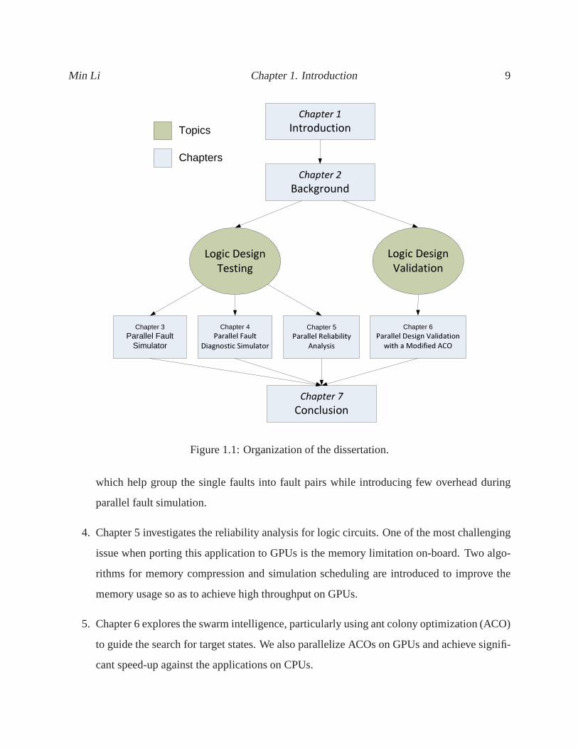
1.3 Dissertation Organization
This dissertation is organized according to the areas illustrated in Fig. 1.1.
1. Chapter 2 introduces the fundamentals of Graphic Processing Units, including its hardware
architecture, memory hierarchy, and programming environment. Meanwhile, the fault model
used in our work and basic knowledge of fault simulation is also presented.
2. Chapter 3 discusses the implementation of fault simulation on GPUs. The novel three-
dimensional parallelism on the GPUs is presented. We demonstrate the improvement achieved
by exploiting compact gate and GPU oriented optimization. In addition, a dynamic load bal-
ancing technique is introduced for further performance improvement.
3. Chapter 4 presents a two-step framework for the parallel diagnostic fault simulation on
GPUs. We demonstrate that the fault pair based fault diagnostic simulation could be effi-
ciently parallelized on GPUs. Also, we propose a novel idea of multiple fault signatures
Min Li Chapter 1. Introduction 9
Chapter 1
Introduction
Logic Design
Testing
Logic Design
Validation
Chapter 3Parallel Fault
Simulator
Chapter 4Parallel Fault
Diagnostic Simulator
Chapter 5Parallel Reliability
Analysis
Chapter 2
Background
Chapter 6Parallel Design Validation
with a Modified ACO
Chapters
Topics
Chapter 7
Conclusion
Figure 1.1: Organization of the dissertation.
which help group the single faults into fault pairs while introducing few overhead during
parallel fault simulation.
4. Chapter 5 investigates the reliability analysis for logic circuits. One of the most challenging
issue when porting this application to GPUs is the memory limitation on-board. Two algo-
rithms for memory compression and simulation scheduling are introduced to improve the
memory usage so as to achieve high throughput on GPUs.
5. Chapter 6 explores the swarm intelligence, particularlyusing ant colony optimization (ACO)
to guide the search for target states. We also parallelize ACOs on GPUs and achieve signifi-
cant speed-up against the applications on CPUs.
Min Li Chapter 1. Introduction 10
6. Chapter 7 concludes the dissertation. It summarizes the initial attempts for accelerating
applications in two major EDA areas: digital design testingand Validation using the state-
of-the-art many-core system, graphics processing units.
Chapter 2
Background
In this chapter, we present the hardware platform we used in our implementation, which is NVIDIA
GeForce 285 GTX device. The hardware architecture, memory hierarchy and programming model
will be described in order to provide the background of GPU platform. Also, the concepts related
to logic system testing and validation are introduced.
2.1 Graphic Processing Units
Back in 1999, the notion of GPU was defined and popularized by NVIDIA. The unit was designed
as a specialized chip to accelerate the building of images for display. As displays became more
complex and demanding, the GPU evolved rapidly from a single-core processor to today’s many-
core architecture which is capable of processing millions of polygons per second. This is because
most of the graphical display manipulation tasks such as transform, lighting and rendering, can be
performed independently on different regions of the display. In other words, the same instruction
can simultaneously operate on multiple independent data. Therefore, GPUs were designed as a
parallel system in a Single Instruction Multiple Data (SIMD) fashion.
Recently, GPUs have emerged as an attractive and effective platform for parallel processing, espe-
11
Min Li Chapter 2. Background 12
cially for those data-intensive applications. With enhanced programmability and higher precision
arithmetic, this has coined the term “general purpose processing using GPU (GPGPU).” [33, 60,
74, 81]. The popularity of GPGPU stems from the following.
1. Large dedicated graphics memories. Our NVIDIA GTX285 graphic card is equipped with
1 GB DDR3 dedicated graphics memory. With large size of memories, more data could be
placed on the GPUs and intuitively higher levels of parallelism could be achieved.
2. High memory bandwidth. The reason that GPU is extremely memory intensive is because
that the dedicated graphics memories guaranteed a high memory bandwidth. The intercon-
nect between the memory and the GPU processors supports veryhigh bandwidth of up to
159.0 GB/s. While the conventional CPU is only 16 GB/s, whichtranslates to around 10
times slower.
3. High Computational power. With more than 200 hundred processing units under a highly
pipelined and parallel architecture, GTX285 could achievemore than 1000 GFlops in single
precision.
4. Availability. GPUs card are available off-the-shelf devices equipped in every desktops and
even laptops. And also, it is relatively inexpensive considering its computational power.
Several years ago, the GPU was a fixed-function processor designed for a particular class of appli-
cations. Over the past few years, the GPU has evolved into a powerful programmable processor,
with application programming interface (APIs). One of the most popular one is the Compute Uni-
fied Device Architecture (CUDA) provided by NVIDIA which abstracts away the hardware details
and makes the GPUs become accessible for computation like CPUs [72]. Also, CUDA provides
developers access to the virtual instruction set the memoryin GPUs.
The interaction between the host (CPU) and the device (GPU) in the paradigm of CUDA is shown
in Figure 2.1. The right part is the device portion which consists of a many-core GPU and the
dedicated memory on-board. GPUs can directly read and writefrom its own memory. The graphics
Min Li Chapter 2. Background 13
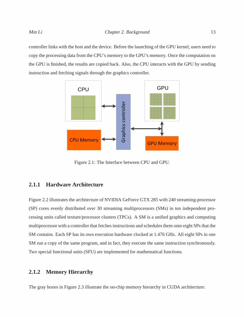
controller links with the host and the device. Before the launching of the GPU kernel, users need to
copy the processing data from the CPU’s memory to the GPU’s memory. Once the computation on
the GPU is finished, the results are copied back. Also, the CPUinteracts with the GPU by sending
instruction and fetching signals through the graphics controller.
CPU GPU
CPU MemoryGPU Memory
Gra
ph
ics
co
ntr
oll
er
Figure 2.1: The Interface between CPU and GPU.
2.1.1 Hardware Architecture
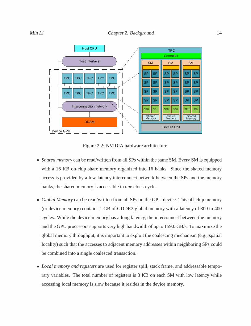
Figure 2.2 illustrates the architecture of NVIDIA GeForce GTX 285 with 240 streaming-processor
(SP) cores evenly distributed over 30 streaming multiprocessors (SMs) in ten independent pro-
cessing units called texture/processor clusters (TPCs). ASM is a unified graphics and computing
multiprocessor with a controller that fetches instructions and schedules them onto eight SPs that the
SM contains. Each SP has its own execution hardware clocked at 1.476 GHz. All eight SPs in one
SM run a copy of the same program, and in fact, they execute thesame instruction synchronously.
Two special functional units (SFU) are implemented for mathematical functions.
2.1.2 Memory Hierarchy
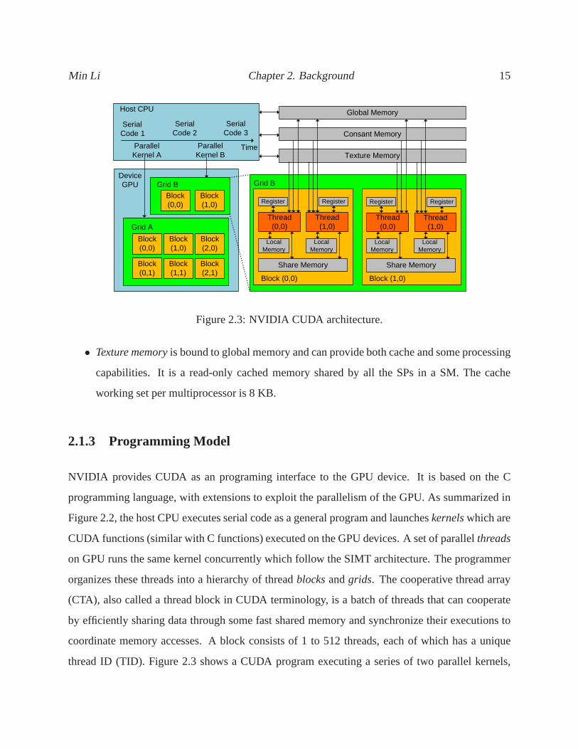
The gray boxes in Figure 2.3 illustrate the on-chip memory hierarchy in CUDA architecture:
Min Li Chapter 2. Background 14
SP SP
SP SP
SP SP
SP SP
SFU SFU
SharedMemory
Controller
SM
SP SP
SP SP
SP SP
SP SP
SFU SFU
SharedMemory
SM
Texture Unit
TPC
TPC
DRAM
Interconnection network
TPC TPC TPCTPC
Device GPU
Host Interface
Host CPU
SP SP
SP SP
SP SP
SP SP
SFU SFU
SharedMemory
SM
TPC TPC TPC TPCTPC
Figure 2.2: NVIDIA hardware architecture.
• Shared memorycan be read/written from all SPs within the same SM. Every SM is equipped
with a 16 KB on-chip share memory organized into 16 banks. Since the shared memory
access is provided by a low-latency interconnect network between the SPs and the memory
banks, the shared memory is accessible inoneclock cycle.
• Global Memorycan be read/written from all SPs on the GPU device. This off-chip memory
(or device memory) contains 1 GB of GDDR3 global memory with alatency of 300 to 400
cycles. While the device memory has a long latency, the interconnect between the memory
and the GPU processors supports very high bandwidth of up to 159.0 GB/s. To maximize the
global memory throughput, it is important to exploit the coalescing mechanism (e.g., spatial
locality) such that the accesses to adjacent memory addresses within neighboring SPs could
be combined into a single coalesced transaction.
• Local memory and registersare used for register spill, stack frame, and addressable tempo-
rary variables. The total number of registers is 8 KB on each SM with low latency while
accessing local memory is slow because it resides in the device memory.
Min Li Chapter 2. Background 15
DeviceGPU
Block(0,0)
Block(1,0)
Grid A
Grid B
Host CPU
Parallel Kernel A
Parallel Kernel B
Thread (0,0)
Block (0,0)
Block(1,0)
Block(0,0)
Thread (1,0)
Grid B
Thread (0,0)
Block (1,0)
Thread (1,0)
Register
Global Memory
Share Memory
Local Memory
Register
Consant Memory
Texture Memory
Local Memory
Share Memory
Local Memory
Local Memory
RegisterRegister
Block(2,0)
Block(0,1)
Block(1,1)
Block(2,1)
Serial Code 1
Serial Code 2
Time
Serial Code 3
Figure 2.3: NVIDIA CUDA architecture.
• Texture memoryis bound to global memory and can provide both cache and some processing
capabilities. It is a read-only cached memory shared by all the SPs in a SM. The cache
working set per multiprocessor is 8 KB.
2.1.3 Programming Model
NVIDIA provides CUDA as an programing interface to the GPU device. It is based on the C
programming language, with extensions to exploit the parallelism of the GPU. As summarized in
Figure 2.2, the host CPU executes serial code as a general program and launcheskernelswhich are
CUDA functions (similar with C functions) executed on the GPU devices. A set of parallelthreads
on GPU runs the same kernel concurrently which follow the SIMT architecture. The programmer
organizes these threads into a hierarchy of threadblocksandgrids. The cooperative thread array
(CTA), also called a thread block in CUDA terminology, is a batch of threads that can cooperate
by efficiently sharing data through some fast shared memory and synchronize their executions to
coordinate memory accesses. A block consists of 1 to 512 threads, each of which has a unique
thread ID (TID). Figure 2.3 shows a CUDA program executing a series of two parallel kernels,
Min Li Chapter 2. Background 16
KernelA and KernelB on a heterogeneous CPU-GPU system. In this figure, KernelA executes on
the GPU as a grid of 6 blocks; KernelB executes on the GPU as a grid of two blocks, with 2 threads
instantiated per block.
Relevant to the GPU hardware architecture described in Section 2.1.1, one thread block could be
allocated to exactly one SM, while one SM executes up to eightblocks concurrently, depending
on the demand for resources. When an MP is assigned to executeone or more thread blocks, the
controller splits and creates groups of parallel threads calledwarps. CUDA defines the termwarp, a
group of32 threads which are created, managed, scheduled and executedconcurrently on the same
SM. Since the threads in a warp have the same instruction execution schedule, such a processor
architecture is called single-instruction, multiple-thread (SIMT). It is noted that threads in the same
warp can follow different instruction paths which is calledbranch divergence. However, branch
divergence can drastically reduce the performance becausethe warp must serially execute each
branch path taken, thereby disabling those threads that arenot on the same path. In other words,
only the threads that follow the same execution path can be processed in parallel, while the disabled
threads must wait until all the threads converge back to the same path. Each warp will synchronize
all the threads as they converge back to the same path. Our works achieve full efficiency because
all 32 threads of a warp always agree on their execution path throughout the program.
2.1.4 Applications
Recent research shows that the GPU computing density improves faster than the CPU [75]. It
has been shown that a massive array of GPU cores could offer anorder of magnitude higher raw
computation power than the CPU.
Signal and image processing is the initial area that GPU was targeted; FFT computation and matrix
manipulation for image rendering. With the advances of GPUs, researchers also investigate the
filed of cryptography. Authors in [62] first implement an efficient Advanced Encryption Standard
(AES) algorithms using CUDA. The developed solutions run upto 20 times faster than OpenSSL
Min Li Chapter 2. Background 17
and in the same range of performance of existing hardware based implementations. Besides the
symmetric cryptography, asymmetric cryptography such as RSA and DSA crypto-systems as well
as Elliptic Curve Cryptography (ECC) are studied in [92]. Using NVIDIA 8800GTS graphics
card, they are able to compute 813 modular exponentiations per second for RSA or DSA-based
systems with 1024 bit integers. Moreover, the design for ECCover the prime field even achieves
the throughput of 1412 point multiplications per second.
Like many other software communities, the networking area also needs an overhaul of computa-
tional power so as to keep pace with the ever increasing networking complexity. It is thus appealing
to unleash the computing power of GPU for networking applications [36, 42, 9]. PacketShader,
a high-performance software router framework for general packet processing acceleration is pro-
posed in [42]. The authors implemented IPv4 and IPv6 forwarding, OpenFlow switching, and
IPsec tunneling to demonstrate the flexibility and performance advantage of PacketShader. Com-
bined with their high-performance packet I/O engine, PacketShader outperforms existing software
routers by more than a factor of four, forwarding 64B IPv4 packets at 39 Gbps on a single com-
modity PC. An immature idea of upgrading NS-2 simulator using GPGPU is proposed in [36].
Although no experimental results are given in the paper, theauthors claimed that if they can ac-
celerate the propagation model, the gained speedup could have a significant value for large scale
networks. Researches in [9] implemented a similar idea to accelerate a discrete-event parallel net-
work simulator, PRIME SSFNet using GPUs. Basically, GPUs are used to perform ray-tracing at
high speeds to facilitate propagation modeling based on geometric optics. On average, the pro-
posed system with four GPUs and a CPU achieves a throughput five times faster than a single
GPU.
Data mining algorithms are an integral part of a wide varietyof commercial applications such as
online searching, shopping and social network systems. Many of these applications analyze large
volumes of online data and are highly computation and memory-intensive. As a result, researchers
have been actively seeking new techniques and architectures to improve the query execution time.
In [37], data is streamed to and from the GPU in real time and the blending and texture mapping
functionalities of GPUs are exploited. The experimental results demonstrate a speedup of 2-5 times
Min Li Chapter 2. Background 18
over high-end CPU implementations.
The advent of GPGPU also brought new opportunities for speeding up time-consuming electronic
design automation (EDA) applications [29, 38, 39, 21, 20, 47, 67]. The authors in [38, 47] are the
pioneers who parallelized EDA algorithms on GPUs. They exploited both fault parallelism and
pattern parallelism provided by GPUs and implemented an efficient fault simulator. Also, efficient
gate level logic simulators are proposed by authors in [21, 20] where the circuits are partitioned into
independent portions and processed among blocks in parallel. Besides the gate level simulators, a
GPU based System-C simulator is introduced in [67]. The discrete-event simulation is parallelized
on the GPU by transforming the model of computation into a model of concurrent threads that
synchronize as and when necessary. The GPU-based applications for EDA community are not
restricted to simulators. Since the irregular data access patterns are determined by the very nature
of VLSI circuits, authors in [29] accelerated sparse matrixmanipulations and graph algorithms on
GPUs which have widely been used in EDA tools.
2.2 Digital Systems Testing
2.2.1 Single Stuck at Fault Model
Logical faults represent the effect of physical defects on the behavior of the modeled system.
Unless explicitly stated, most of the literature in the testing area assumes that at most one fault is
present in the system, since multiple faults are generally much easier to detect. This single-fault
assumption significantly simplifies the test generation problem. Practically, even when multiple
faults are present, the test derived under the single-faultassumption is usually applicable for the
detection of multiple faults by composing the individual tests designed for each single fault.
Some well-known fault models are the single stuck-at fault (SSF), bridging fault, and delay fault.
In this dissertation, we target the single stuck-at fault model, the simplest but most widely used
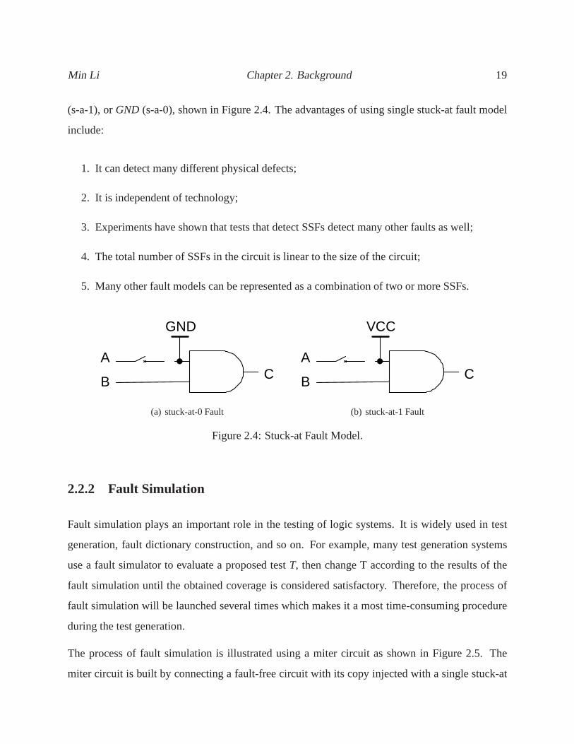
fault model. The effect of the single stuck-at fault is as if the faulty node is tied to eitherVCC
Min Li Chapter 2. Background 19
(s-a-1), orGND (s-a-0), shown in Figure 2.4. The advantages of using singlestuck-at fault model
include:
1. It can detect many different physical defects;
2. It is independent of technology;
3. Experiments have shown that tests that detect SSFs detectmany other faults as well;
4. The total number of SSFs in the circuit is linear to the sizeof the circuit;
5. Many other fault models can be represented as a combination of two or more SSFs.
A
B
GND
C
(a) stuck-at-0 Fault
A
B
VCC
C
(b) stuck-at-1 Fault
Figure 2.4: Stuck-at Fault Model.
2.2.2 Fault Simulation
Fault simulation plays an important role in the testing of logic systems. It is widely used in test
generation, fault dictionary construction, and so on. For example, many test generation systems
use a fault simulator to evaluate a proposed testT, then change T according to the results of the
fault simulation until the obtained coverage is consideredsatisfactory. Therefore, the process of
fault simulation will be launched several times which makesit a most time-consuming procedure
during the test generation.
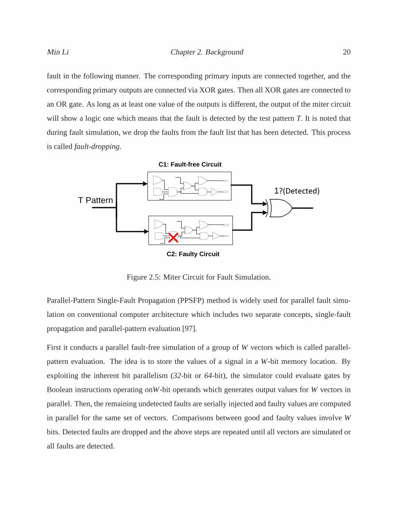
The process of fault simulation is illustrated using a mitercircuit as shown in Figure 2.5. The
miter circuit is built by connecting a fault-free circuit with its copy injected with a single stuck-at
Min Li Chapter 2. Background 20
fault in the following manner. The corresponding primary inputs are connected together, and the
corresponding primary outputs are connected via XOR gates.Then all XOR gates are connected to
an OR gate. As long as at least one value of the outputs is different, the output of the miter circuit
will show a logic one which means that the fault is detected bythe test patternT. It is noted that
during fault simulation, we drop the faults from the fault list that has been detected. This process
is calledfault-dropping.
C2: Faulty Circuit
C1: Fault-free Circuit
1?(Detected)T Pattern
Figure 2.5: Miter Circuit for Fault Simulation.
Parallel-Pattern Single-Fault Propagation (PPSFP) method is widely used for parallel fault simu-
lation on conventional computer architecture which includes two separate concepts, single-fault
propagation and parallel-pattern evaluation [97].
First it conducts a parallel fault-free simulation of a group of W vectors which is called parallel-
pattern evaluation. The idea is to store the values of a signal in a W-bit memory location. By
exploiting the inherent bit parallelism (32-bit or 64-bit), the simulator could evaluate gates by
Boolean instructions operating onW-bit operands which generates output values forW vectors in
parallel. Then, the remaining undetected faults are serially injected and faulty values are computed
in parallel for the same set of vectors. Comparisons betweengood and faulty values involveW
bits. Detected faults are dropped and the above steps are repeated until all vectors are simulated or
all faults are detected.
Min Li Chapter 2. Background 21
2.2.3 Reliablity Analysis
CMOS scaling has taken us to the nanometer-range feature sizes. In addition, non-conventional
nanotechnologies are currently being investigated as potential alternatives to CMOS. Although
nano-scale circuits offer low power consumption and high switching speed, they are expected to
have higher error rates due to the reduced margins to noise and transients at such small dimensions.
The errors that arise due to temporary deviation or malfunction of nano-devices can be character-
ized as probabilistic errors, each of which is an intrinsic property of each device. Such errors are
hard to detect by regular testing methodologies because they may occur anywhere in the circuit
and are not permanent defects. Thus, each devicei (logic gate or interconnect) will have a cer-
tain probability of errorτi ∈ [0, 0.5], which cause its output to flip symmetrically (from0 → 1
or 1 → 0). A common fault model of a circuit withn gates is defined as the failure probability
~τ = {τ1, τ2, . . . , τn}, whereτk is the failure probabilities of thekth gate. In our experiments, we
assign an universal error rate (failure probability) to allthe gates for simplicity. However, RAG is
able to consider gates with different error rates.
The reliability of logic circuits could be evaluated by several measures. Suppose we have a logic
circuit with m outputs. In [24], the probability of errors for each outputi, denoted asδi, is em-
ployed. Among them outputs, the maximum probability of error,maxmi=1(δi) is used in [86]
and authors in [22] utilized the average reliability value,summi=1(1 − δi)/m. The authors using
PTMs [49] proposedFidelity, denoted asF , which is the probability that the entire circuit is func-
tionally correct (allm outputs are fault free). They also employed the average reliability among
outputs (Ravg) which is also the metric we used in this work.
Min Li Chapter 2. Background 22
2.3 Digital Systems Validation
2.3.1 State Justification
The complexity of current designs makes it hard to generate effective vectors for covering corner
cases. An example corner case is a hard-to-reach state needed to detect a fault or prove a property.
Despite the advances made over the years, state justification remains to be one of the hardest
tasks in sequential ATPG and design validation. In this section, we presents background of status
justification.
Definition 1. For a digital circuit with m inputs andn Flip-Flops (FFs), the state space and
the primary inputs (PIs) are defined by indexed sets of Boolean variablesV = {v1, . . . , vn} and
W = {w1, . . . , wm} respectively, wherevi/wj denotes for the logic value (q∈{0, 1}) of the ith
Flip-Flop / jth PI.
Let V ′ = {v′1, . . . , v′
n} be the next state variables, then the next state function canbe expressed
asV ′ = δ(V,W ). Based on the next state function, a transition relationT (V,W, V ′) can be
constructed such thatT (V,W, V ′) = 1 iff V ′ = δ(V,W ).
For the variables in time framet, we useV t = {vt1, . . . , vtn} andW t = {wt
1, . . . , wtn}. Particu-
larly, the initial state is denoted byV 0 and target state isV f . Also, a sequence of input vectors
W i,W i+1, . . . ,W j can be represented asW i...j wheni≤j. Similarly for state variablesV .
Definition 2. For a sequential circuit, transitions among states can be illustrated by a directed
graphG(N,E), namely the State Transition Graph (STG), with the nodes setN = {V 0, V 1 . . .}
and the edge setE = {eV iV j |V i, V j∈V, ∃W s.t. V j = δ(V i,W )}.
Based on the STG, the process of state justification can be formulated as a process of searching for
a directed path from vertexV 0 to V f in G(N,E). Such a path with lengtht can be expressed as a
sequence of inputs:W 0...t which satisfies the Boolean equation:
V 0 ∧∧t−1
i=0T (V i,W i, V i+1) ∧ V f (2.1)
Min Li Chapter 2. Background 23
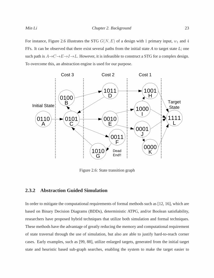
For instance, Figure 2.6 illustrates the STGG(N,E) of a design with1 primary input,w1 and4
FFs. It can be observed that there exist several paths from the initial stateA to target stateL; one
such path isA→C→E→I→L. However, it is infeasible to construct a STG for a complex design.
To overcome this, an abstraction engine is used for our purpose.
1111
0000
0001
1001
1000
001001010110
0011
1010
Cost 1Cost 2Cost 3
Dead End!!
01001011
Initial StateTarget State
A
B
C
G
D
E
F
K
J
I
H
L
Figure 2.6: State transition graph
2.3.2 Abstraction Guided Simulation
In order to mitigate the computational requirements of formal methods such as [12, 16], which are
based on Binary Decision Diagrams (BDDs), deterministic ATPG, and/or Boolean satisfiability,
researchers have proposed hybrid techniques that utilize both simulation and formal techniques.
These methods have the advantage of greatly reducing the memory and computational requirement
of state traversal through the use of simulation, but also are able to justify hard-to-reach corner
cases. Early examples, such as [99, 88], utilize enlarged targets, generated from the initial target
state and heuristic based sub-graph searches, enabling thesystem to make the target easier to
Min Li Chapter 2. Background 24
reach. However, as circuit complexity grew, these methods became computationally infeasible
due to memory explosion in finding an enlarged target, and with the explosion of subgraphs to be
checked in local model checking. To handle these limitations, researchers introduced abstraction
guided simulation, which utilizes formal techniques to create a simplified model of the behavior of
the circuit state variables [28, 78, 90].
The concept of a distance based cost function abstraction was proposed by the authors of [90]. This
cost function abstraction interacts closely with the target state allowing for customization of the
abstraction for each property to be verified. Additionally,[78] provided a method of abstraction
refinement using data-mining to aid a GA-based search engine. However, in both cases, it is still
sometimes difficult to guide the search through narrow statepaths without the use of a BMC. The
authors of [28] propose the method of buckets representing the distance of the states they contain
from the abstracted target state. In such a method, after each state has been simulated, the program
flips a fair coin to determine if it should continue simulation or backtrack to a different ring.
While such an approach avoids some local minima, some statesremain hard-to-reach. Finally, [53]
proposes the use of ACOs for solving the state justification problem utilizing an abstraction cost
function as a heuristic the ACO guides the search and limits the input space based on information
discovered during runtime.
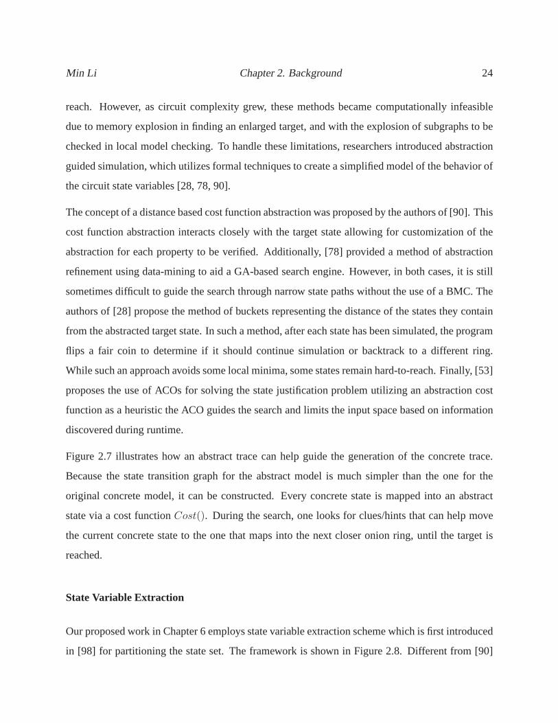
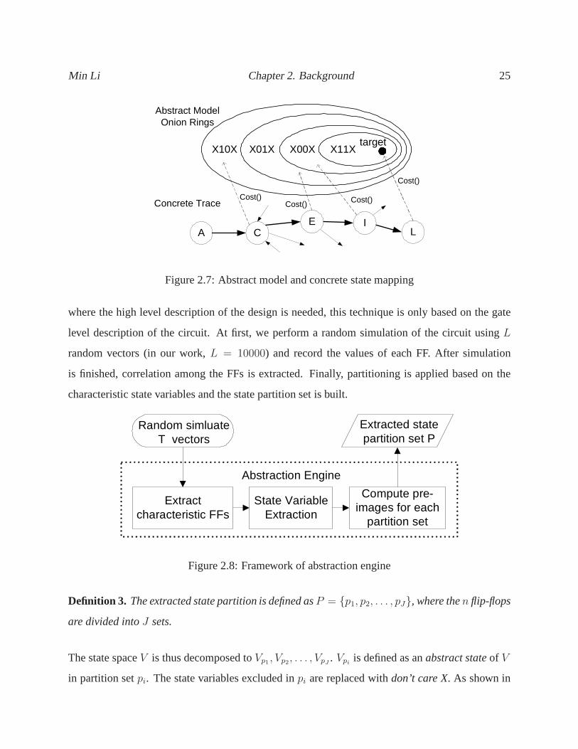
Figure 2.7 illustrates how an abstract trace can help guide the generation of the concrete trace.
Because the state transition graph for the abstract model ismuch simpler than the one for the
original concrete model, it can be constructed. Every concrete state is mapped into an abstract
state via a cost functionCost(). During the search, one looks for clues/hints that can help move
the current concrete state to the one that maps into the next closer onion ring, until the target is
reached.
State Variable Extraction
Our proposed work in Chapter 6 employs state variable extraction scheme which is first introduced
in [98] for partitioning the state set. The framework is shown in Figure 2.8. Different from [90]
Min Li Chapter 2. Background 25
X11XX00XX01XX10X
Abstract ModelOnion Rings
A
Concrete Trace
target
Cost()Cost() Cost()
Cost()
CE I
L
Figure 2.7: Abstract model and concrete state mapping
where the high level description of the design is needed, this technique is only based on the gate
level description of the circuit. At first, we perform a random simulation of the circuit usingL
random vectors (in our work,L = 10000) and record the values of each FF. After simulation
is finished, correlation among the FFs is extracted. Finally, partitioning is applied based on the
characteristic state variables and the state partition setis built.
Extract characteristic FFs
Compute pre-images for each
partition set
State Variable Extraction
Abstraction Engine
Extracted state partition set P
Random simluate T vectors
Figure 2.8: Framework of abstraction engine
Definition 3. The extracted state partition is defined asP = {p1, p2, . . . , pJ}, where then flip-flops
are divided intoJ sets.
The state spaceV is thus decomposed toVp1 , Vp2, . . . , VpJ . Vpi is defined as anabstract stateof V
in partition setpi. The state variables excluded inpi are replaced withdon’t care X. As shown in
Min Li Chapter 2. Background 26
X11XX00XX01XX10X
1XX1
0XX0
1XX0
0XX1
Preimage(FF2,FF3) Preimage(FF1,FF4)
d=1 d=1d=2d=3
1010 Concrete State
Cost(S)=max(2,1)=2
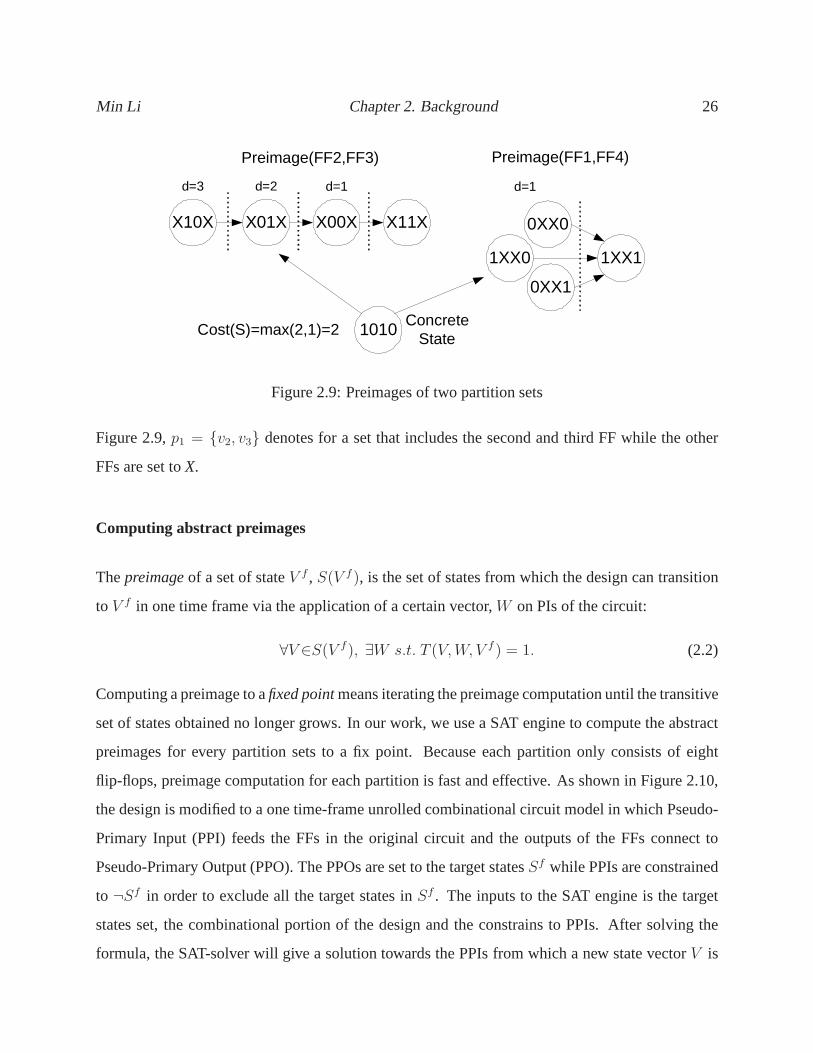
Figure 2.9: Preimages of two partition sets
Figure 2.9,p1 = {v2, v3} denotes for a set that includes the second and third FF while the other
FFs are set toX.
Computing abstract preimages
Thepreimageof a set of stateV f , S(V f ), is the set of states from which the design can transition
to V f in one time frame via the application of a certain vector,W on PIs of the circuit:
∀V ∈S(V f), ∃W s.t. T (V,W, V f ) = 1. (2.2)
Computing a preimage to afixed pointmeans iterating the preimage computation until the transitive
set of states obtained no longer grows. In our work, we use a SAT engine to compute the abstract
preimages for every partition sets to a fix point. Because each partition only consists of eight
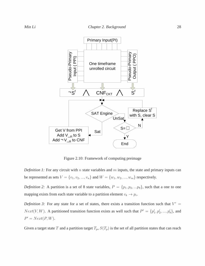
flip-flops, preimage computation for each partition is fast and effective. As shown in Figure 2.10,
the design is modified to a one time-frame unrolled combinational circuit model in which Pseudo-
Primary Input (PPI) feeds the FFs in the original circuit andthe outputs of the FFs connect to
Pseudo-Primary Output (PPO). The PPOs are set to the target statesSf while PPIs are constrained
to ¬Sf in order to exclude all the target states inSf . The inputs to the SAT engine is the target
states set, the combinational portion of the design and the constrains to PPIs. After solving the
formula, the SAT-solver will give a solution towards the PPIs from which a new state vectorV is
Min Li Chapter 2. Background 27
assigned. The new state vector is called the 1-step preimageof the states inSf . For each partition
setpj , we addV fpj
to setS as well as its complement to PPIs and run the SAT engine again.The
procedure is repeated until the instance is unsatisfiable (UNSAT) which means that all possible
1-step preimage solutions ofSf is contained inS. Then, we replaceSf with S and compute the
preimages in next time frame. The process is terminated whenS = ∅ which means that all the
abstract states are obtained for partitionpj .
The size of each partition setpi is experimentally limited to a maximum of8 variables. Thus, the
number of distinct abstract states in one group is at most256 which makes preimage computation
very lightweight. At the same time, abstract groups of8 state variables are demonstrated to be
effective for guidance according to our experimental results.
Preimages of two partition sets(FF2, FF3) and(FF1, FF4) are shown in Figure 2.9.
Definition 4. The distance of a stateV in partition setpj, d(Vpj) is defined as the number of time
frames it takes fromVpj to V fpj
.
Using Figure 2.9 again, the distance between state1010 and the target is2 for the partition set
{p2, p3} and1 for {p1, p4}. By partitioning the state space as in [98], we can find abstract groups
that are highly related to the target. Thus, more useful approximate distances can be obtained. For
example, the partition set{p2, p3} is more favorable than{p1, p4} because the abstract distance in
set{p2, p3} is more accurate when compared to the concrete model.
2.3.3 Partition Navigation Tracks
Partition Navigation Tracks (PNTs) represent the cost function used as our heuristic. A pictorial
representation is shown in Fig. 2.7. A PNT is generated for each flip-flop partition utilizing a SAT
engine. The SAT engine is fed a set of clauses defining the behavior of the circuit as well as the
values of the flip-flops of the partition in the target state. To facilitate the discussion on generating
PNTs, the following definitions are needed.
Min Li Chapter 2. Background 28
UnSat
One timeframe unrolled circuit
Primary Input(PI)
Pse
udo-
Prim
ary
Out
put (
PP
O)
Pse
udo-
Prim
ary
Inpu
t ( P
PI)
CNFCKT Sf
SAT Engine
End
Sat
Sf
Get V from PPIAdd V_pj to S
Add V_pj to CNF
Replace Sf
with S, clear S
∅
Y
NS=
¬
¬
Figure 2.10: Framework of computing preimage
Definition 1: For any circuit withn state variables andm inputs, the state and primary inputs can
be represented as setsV = {v1, v2, ..., vn} andW = {w1, w2, ..., wm} respectively.
Definition 2: A partition is a set of 8 state variables,P = {p1, p2, ...p8}, such that a one to one
mapping exists from each state variable to a partition element vk → pi.
Definition 3: For any state for a set of states, there exists a transition function such thatV ′ =
Next(V,W ). A partitioned transition function exists as well such thatP ′ = {p′1, p′
2, ..., p′
8}, and
P ′ = Next(P,W ).
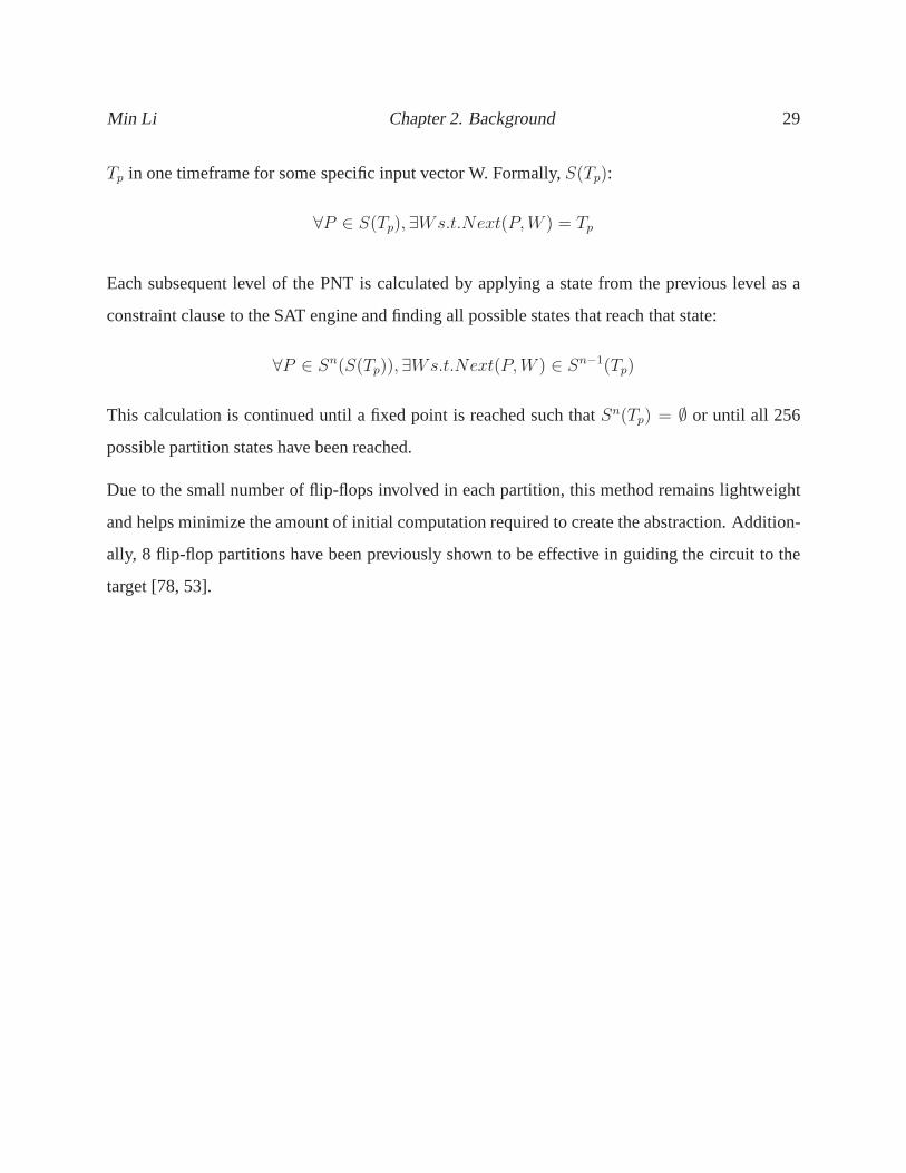
Given a target stateT and a partition targetTp, S(Tp) is the set of all partition states that can reach
Min Li Chapter 2. Background 29
Tp in one timeframe for some specific input vector W. Formally,S(Tp):
∀P ∈ S(Tp), ∃Ws.t.Next(P,W ) = Tp
Each subsequent level of the PNT is calculated by applying a state from the previous level as a
constraint clause to the SAT engine and finding all possible states that reach that state:
∀P ∈ Sn(S(Tp)), ∃Ws.t.Next(P,W ) ∈ Sn−1(Tp)
This calculation is continued until a fixed point is reached such thatSn(Tp) = ∅ or until all 256
possible partition states have been reached.
Due to the small number of flip-flops involved in each partition, this method remains lightweight
and helps minimize the amount of initial computation required to create the abstraction. Addition-
ally, 8 flip-flop partitions have been previously shown to be effective in guiding the circuit to the
target [78, 53].
Chapter 3
Parallel Fault Simulator
3.1 Chapter Overview
In this chapter, we present an efficient parallel fault simulator, FSimGP2, that exploits the high de-
gree of parallelism supported by a state-of-the-art graphic processing unit with the NVIDIA Com-
pute Unified Device Architecture. A novel three-dimensional parallel fault simulation technique is
proposed to achieve extremely high computation efficiency on the GPU. Global communication is
minimized by concentrating as much work as possible on the local device’s memory. We present
results on a GPU platform from NVIDIA (a GeForce GTX 285 graphics card) that demonstrate a
speedup of up to 63× and 4× compared to another two GPU-based fault simulators and up to95×
over a state-of-the-art algorithm on conventional processor architectures.
The rest of the chapter is organized as follows. A brief introduction is given in Section 3.2. In
Section 3.3, we review the previous work in the area of GPU-based parallel application for fault
simulation. Section 3.4 outlines a high-level process viewof the proposed view of FSimGP2. The
experimental results are reported in Section 3.5. Finally Section 3.6 concludes the chapter.
30
Min Li Chapter 3. Parallel Fault Simulator 31
3.2 Introduction
Fault Simulation, a process of simulating the response of a circuit-under-test under a set of test-
ing patterns in the presence of modeled faults, plays an important role to various applications in
very-large-scale integration circuit test including Automatic Test Pattern Generation, built-in self-
test, testability analysis, etc. In the past several decades, significant efforts have been devoted to
accelerate this process [51, 71, 87]. However, with the advances in current VLSI technology, more
devices can be placed on a single chip. As a result, there is a need for efficient fault simulators that
are able to handle large designs with extremely large test sets. In addition to test-related applica-
tions, simulation of a large number of test patterns can alsobenefit many other applications. Fast
(fault) simulators would thus offer tremendous benefit.
In order to alleviate the simulation bottleneck, researchers have proposed several parallel process-
ing approaches by exploiting the power of supercomputers, dedicated hardware accelerates and
vector machines. These techniques can be divided into threemain classes:
1. Algorithm Parallelism. Different tasks such as logic gate evaluation, scheduling and in-
put/output processing are preformed in a pipelined fashionand distributed to dedicated pro-
cessors. Thus, by functional partitioning of simulation algorithms, the communication and
synchronization between processors can be reduced [3, 66, 7, 5].
2. Model Parallelism.The gate-level netlist of the CUT is partitioned into several components.
Since each sub-circuit can be simulated independently, different elements are computed by
several processors in parallel [69, 79, 80, 93].
3. Data Parallelism. In fault simulation, either multiple patterns and/or multiple faults can
be processed independently on one of the processors [6, 10, 43, 46, 76, 77, 84]. Tech-
niques where sets of input vectors (faults) are simulated inparallel are calledfault-parallel
(pattern-parallel). Since there is no data dependence between processors, data parallelism
is particularly attractive for our implementation using Graphics Processing Units.
Min Li Chapter 3. Parallel Fault Simulator 32
In this chapter, we present a novel three-dimensional parallel fault simulator, called FSimGP2 -
Fault Simulator with GPGPU. The main motivation behind thiswork is to harness the computa-
tional power of modern day GPUs to reduce the total executiontime of fault simulation without
compromising the output fidelity. Our method exploits block-, fault- and pattern- parallelism to-
gether which is capable of efficiently utilizing memory bandwidth and massive data parallelism
on the GPU. The overhead of data communication between the host (CPU) and the device (GPU)
is minimized by utilizing as much of the individual device’smemory as possible. FSimGP2 also
takes advantage of the inherent bit-parallelism of logic operations on computer words. In addition,
a clever organization of data structures is developed to exploit the memory hierarchy character-
istic of GPUs. The technique is implemented on the NVIDIA GeForce GTX 285 with 30 cores
and 8 SIMT execution pipelines per core [59]. Our experimental results demonstrate that the pro-
posed FSimGP2 achieves more than three times speedup in comparison with recently developed
GPU-based fault simulators [47] and [38] as well as a state-of-the-art sequential fault simulation
algorithm [51] implemented on conventional processor architecture.
3.3 Background
In this section, we will present the background on parallel fault simulation and previous related
work based on the CUDA architecture.
3.3.1 Fault Simulation
A fault simulator computes an output response of a logic circuit for each given input vector under
each given fault instance. In this work, our proposed approach targets on full-scan gate-level
circuits and assumes the single stuck-at fault model. Our fault simulator is to produce the fault
simulation results for acollapsedfault list in a circuit under a large set of random vectors. In
addition,fault droppingis implemented which means that a fault is removed from the fault list as
soon as it is detected by any test pattern.
Min Li Chapter 3. Parallel Fault Simulator 33
Definition 5. Let V be the total number of test vectors for fault simulation andNf be the number
of collapsed faults. The word size,w, is defined as the number of bits in the computer word. In our
implementation,w equals32. The fault/pattern parallelism factors are defined as variablesp and
t which denote the number of faults/patterns simulated at a time.
Recall that parallelism in fault simulation is classified into fault-parallel and pattern-parallel meth-
ods. The former simulatesp faults for each vector at a time while the latter simulatest patterns
simultaneously for one target fault. Parallelism can be furthered on GPUs by extending word-level
parallelism onto multiple threads. Hence, we now simulatep×w faults ort×w patterns in parallel
by simply extending the simulation unit from one CPU word of sizew to a vector consisting of
p or t words of sizew. Such simulation techniques are referred to asextendedfault- (or pattern-)
parallel simulation.
3.3.2 Previous Work
The authors in [38] give the first attempt to implement fault simulation on GPUs. Both fault
parallelism and pattern parallelism are employed such thateach thread evaluates one gate with
different test vectors as well as different injected faultsin parallel. The gate evaluation is conducted
by a look-up-table (LUT) implemented in the texture memory to exploit the memory bandwidth
of GPUs. Although the proposed implementation could achieve 35× speedup in comparison with
a commercial sequential fault simulator, the computation capacity of the GPU has not been fully
exploited due to two major factors:
1. Transmission Overheadbetween CPUs and GPUs. Since the netlist of the circuit is not
stored on the GPU, the host is responsible for all the scheduling and loading tasks to the
device. Therefore, the performance overhead of data transmission between the host and the
device becomes a major bottleneck. In our work, we try to minimize such communication
overhead by employing a new data structure to store some of the circuit and fault information
on the GPU without causing excessive data transmission.All the simulation workloads are
Min Li Chapter 3. Parallel Fault Simulator 34
processed on the GPU while the CPU is only responsible for providing fundamental data
including circuit netlist, fault lists and collecting fault detection results from the GPU.
2. LUT implemented in the texture memory exploits the extremely large memory bandwidth of
GPUs. However, each thread could only evaluate2 gates with the LUT at a time. Our method
takes advantage of the inherentbit-parallelismof logic operations on computer words on
GPUs. Thus, a packet word of 32 bits can be simulated concurrently such that each thread
could evaluate32 gates simultaneously.
An efficient fault simulator is proposed in [47], which uses the parallel-pattern single-fault propa-
gation (PPSFP) paradigm. It achieves a considerable speedup of 16× compared to a state-of-the-
art fault simulator, FSIM [51]. While PPSFP techniques can prune unnecessary evaluations during
simulation, we believe that the overhead of event scheduling and the cost associated with condi-
tional branches within a warp on the GPU may diminish the gainby exploiting such approaches.
Moreover, in [47], the circuit topology has a strong impact on the performance because the simula-
tor running on GPU canonlyhandle the gates with two inputs. Hence, the speedup may be reduced
for circuits having gates with more than two inputs.
The authors in [20, 21] developed a GPU-accelerated logic simulators under the model-parallelism
scheme. The circuits are partitioned into several clustersand each of them is assigned to a thread
block. Such a model-parallelism algorithm is not applicable for fault simulation because in most
cases, only a small percentage of gates in a circuit are required to be simulated for a specific target
fault. Consequently, the overhead of unnecessary evaluations on unexcited gates might potentially
diminish the gain through computing events in parallel. Ourmethod keeps the fault-free values of
all the gates on the GPU’s device memory and only simulates the elements in the fanout cone of
the faulty gate.
In light of the above discussion, our proposed method introduces a novel three-dimensional parallel
fault simulation technique that avoids all those wasteful simulations and thus maximally harnesses
the GPU’s large memory bandwidth and high computational power. Our method can be applied to
any circuit irrespective of its topology. Moreover, a dynamic load balancing algorithm is proposed
Min Li Chapter 3. Parallel Fault Simulator 35
based on the atomic function provided by CUDA to distribute the workload evenly across the
thread blocks.
3.4 FSimGP2 Architecture
In this section, we first present our three-dimensional parallel fault simulation algorithm. Then
the framework of FSimGP2 is described, followed by the load balancing and memory scalability
techniques.
3.4.1 Three-Dimensional Parallel Fault Simulation
Definition 6. When injecting a faultf onto the circuit, only the gates in the fanout region (FR)
beyond the fault site toward the primary outputs need to be evaluated. We define such set of gates
as FRf and its size assf , which is the number of gates in FRf .
Definition 7. Compact faults set(CFS) is a set of faults with identical FRs. For simplicity, we call
this group of faults acompact fault, represented ascf . The total number of compact faults (cfs)
in the circuit is denoted asNcf , and the size of theith CFS isni, which is the number of collapsed
faults belonging to this CFS.
Figure 3.1 illustrates a CFS whose faulty gate (location) isg1. There are five collapsed, non-
equivalent faults (f1∼f5) included in this CFS. The position of gateg1 in the circuit is shown in
Figure 3.1. It is clear that all these five faults share the same shaded fanout free region. Thus, we
compact these five faults into a compact faultcf which acts as avirtual single faultduring fault
simulation.
In FSimGP2, for a compact faultcf , each gate in the fanout region of compact fault (FRcf ) will
be fault-simulated witht vectors, processed ont threads, wheret is the pattern-parallelism factor
defined before. In Figure 3.1, a compact faultcf is injected on gateg1 and the FRcf is illustrated as
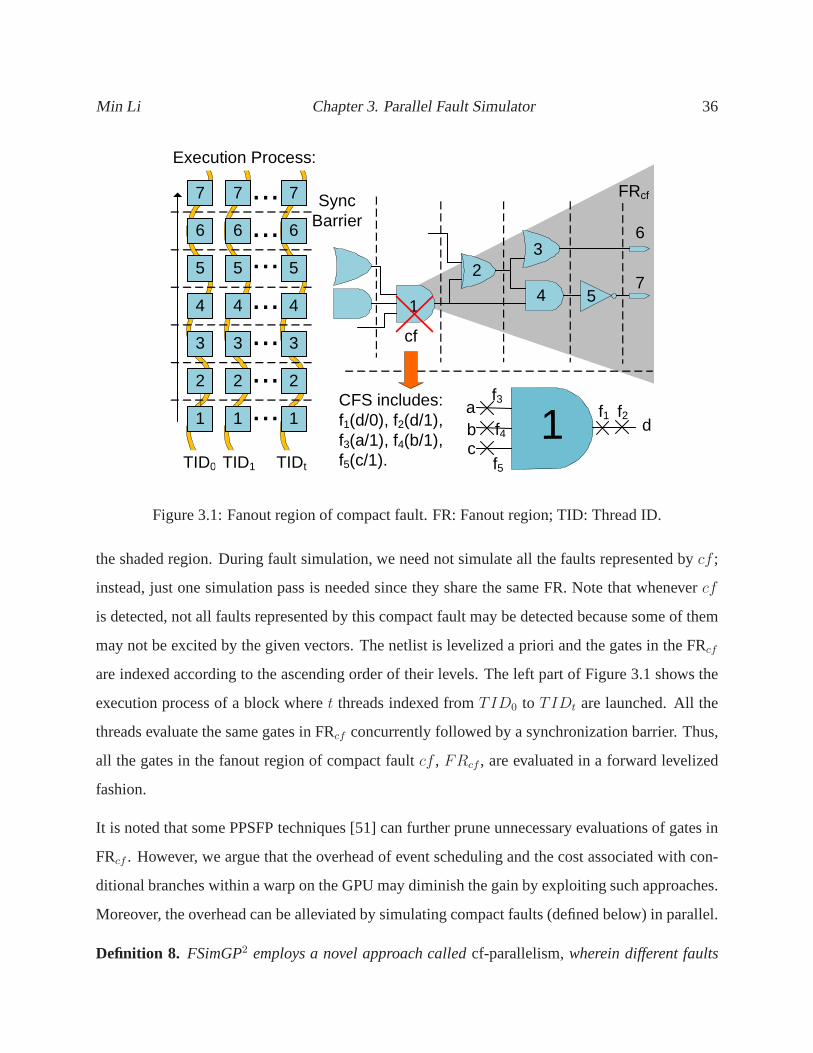
Min Li Chapter 3. Parallel Fault Simulator 36
1
23
4 5
6
7
FRcf
6
5
4
3
2
1
7
6
5
4
3
2
1
7
6
5
4
3
2
1
7
...
TID0 TID1 TIDt
Execution Process:
...
...
...
...
...
...cf
1abc
df1 f2
f3
f5
f4
CFS includes: f1(d/0), f2(d/1), f3(a/1), f4(b/1), f5(c/1).
Sync Barrier
Figure 3.1: Fanout region of compact fault. FR: Fanout region; TID: Thread ID.
the shaded region. During fault simulation, we need not simulate all the faults represented bycf ;
instead, just one simulation pass is needed since they sharethe same FR. Note that whenevercf
is detected, not all faults represented by this compact fault may be detected because some of them
may not be excited by the given vectors. The netlist is levelized a priori and the gates in the FRcf
are indexed according to the ascending order of their levels. The left part of Figure 3.1 shows the
execution process of a block wheret threads indexed fromTID0 to TIDt are launched. All the
threads evaluate the same gates in FRcf concurrently followed by a synchronization barrier. Thus,
all the gates in the fanout region of compact faultcf , FRcf , are evaluated in a forward levelized
fashion.
It is noted that some PPSFP techniques [51] can further pruneunnecessary evaluations of gates in
FRcf . However, we argue that the overhead of event scheduling andthe cost associated with con-
ditional branches within a warp on the GPU may diminish the gain by exploiting such approaches.
Moreover, the overhead can be alleviated by simulating compact faults (defined below) in parallel.
Definition 8. FSimGP2 employs a novel approach calledcf-parallelism, wherein different faults
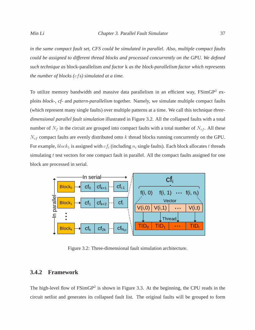
Min Li Chapter 3. Parallel Fault Simulator 37
in the same compact fault set, CFS could be simulated in parallel. Also, multiple compact faults
could be assigned to different thread blocks and processed concurrently on the GPU. We defined
such technique asblock-parallelismand factork as the block-parallelism factor which represents
the number of blocks (cfs) simulated at a time.
To utilize memory bandwidth and massive data parallelism inan efficient way, FSimGP2 ex-
ploits block-, cf- andpattern-parallelismtogether. Namely, we simulate multiple compact faults
(which represent many single faults) over multiple patterns at a time. We call this techniquethree-
dimensional parallel fault simulationillustrated in Figure 3.2. All the collapsed faults with a total
number ofNf in the circuit are grouped into compact faults with a total number ofNcf . All these
Ncf compact faults are evenly distributed ontok thread blocks running concurrently on the GPU.
For example,block1 is assigned withcfi (includingni single faults). Each block allocatest threads
simulatingt test vectors for one compact fault in parallel. All the compact faults assigned for one
block are processed in serial.
In p
aral
lel
Block0 cf0
In serial
Vector
Thread
cfk+1 cfi-1...
Block1 cf1 cfk+2 cfi...
Blockk cfk cf2k cfN...
...
cf
cfif(i, 0) f(i, 1)
V(i,0) V(i,1) V(i,t)
TID0 TID1 TIDt
... f(i, ni)
...
...
Figure 3.2: Three-dimensional fault simulation architecture.
3.4.2 Framework
The high-level flow of FSimGP2 is shown in Figure 3.3. At the beginning, the CPU reads in the
circuit netlist and generates its collapsed fault list. Theoriginal faults will be grouped to form
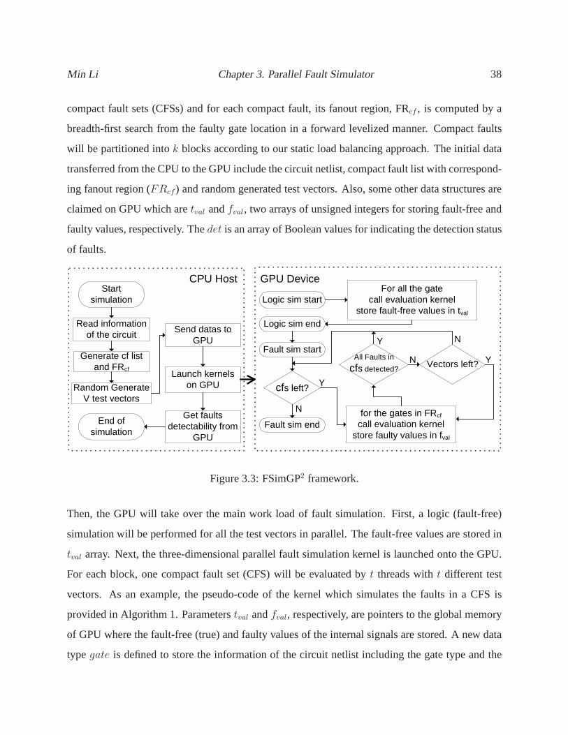
Min Li Chapter 3. Parallel Fault Simulator 38
compact fault sets (CFSs) and for each compact fault, its fanout region, FRcf , is computed by a
breadth-first search from the faulty gate location in a forward levelized manner. Compact faults
will be partitioned intok blocks according to our static load balancing approach. Theinitial data
transferred from the CPU to the GPU include the circuit netlist, compact fault list with correspond-
ing fanout region (FRcf ) and random generated test vectors. Also, some other data structures are
claimed on GPU which aretval andfval, two arrays of unsigned integers for storing fault-free and
faulty values, respectively. Thedet is an array of Boolean values for indicating the detection status
of faults.
Start simulation
End of simulation
Read information of the circuit
Generate cf list and FRcf
Launch kernels on GPU
Get faults detectability from
GPU
Send datas to GPU
for the gates in FRcf
call evaluation kernel store faulty values in fval
For all the gatecall evaluation kernel
store fault-free values in tval
cfs left?
Logic sim start
Logic sim end
Fault sim start
Fault sim end
Vectors left? Y
N
Y
NAll Faults in
cfs detected?
NY
GPU DeviceCPU Host
Random Generate V test vectors
Figure 3.3: FSimGP2 framework.
Then, the GPU will take over the main work load of fault simulation. First, a logic (fault-free)
simulation will be performed for all the test vectors in parallel. The fault-free values are stored in
tval array. Next, the three-dimensional parallel fault simulation kernel is launched onto the GPU.
For each block, one compact fault set (CFS) will be evaluatedby t threads witht different test
vectors. As an example, the pseudo-code of the kernel which simulates the faults in a CFS is
provided in Algorithm 1. Parameterstval andfval, respectively, are pointers to the global memory
of GPU where the fault-free (true) and faulty values of the internal signals are stored. A new data
typegate is defined to store the information of the circuit netlist including the gate type and the
Min Li Chapter 3. Parallel Fault Simulator 39
list of gate inputs. All the gates to be evaluated for the compact fault are stored in an array on the
GPU’s global memory pointed byfr. A gate labelflagalso stored on the global memory indicates
whether a gate is in the FRcf or not. The detection flags forall the single faults are stored in the
det array and transmitted back to the CPU after simulation. At line 1, TID is obtained from the
built-in CUDA variablethreadIdx.x. We do not inject faults on the faulty gate as traditional fault
simulation because different single faults are compacted into the same compact fault (cf ). Here,
we justcomplementthe fault-free values of the faulty gate for allt vectors and store them in thefval
array at line 2. It is noted that the value for a gatei is indexed at a location(TID+i×t) in the value
array. After each gate in the FR is evaluated (line 5), line 6 sets theflag to true indicating that the
gate is in the FR of thecf . Then, we go back to the faulty site and evaluate whether the faults are
excited (line 9). For a single faultf in the CFS that is excited(val⊕tval[tid + fr[0] × t]) and the
faulty value is propagated to one of the primary outputs in the FR(fval[tid+k×t]⊕tval[tid+k×t]),
we set its detection flag to true indicating that the faultf has been detected by the thread (line 11).
After all the threads have finished simulation, a parallel reduction kernel is launched to determine
if the fault is detected by any of thet vectors. Ifall the collapsed faults in the currentcf are
detected, the next compact fault will be processed in the block. Otherwise, anothert test vectors
will be simulated until all theV test vectors have been simulated for the currentcf . If a single fault
is not detected by any vector, we say that the fault is not detected and set its detection flag to false.
In the above discussion, we use an efficient implementation of parallel reduction [11] provided in
CUDA software development kit (SDK) [72].
As illustrated at line 5 of Algorithm 1, depending on thefr[j]’s gate type and the input list available
at gate data structure, theeval kernel will launch a separate kernel to evaluate the faulty value of
the gate. For example, the gate evaluation kernel for fault simulation of a two-input OR gate is
given as a pseudo-code shown in Algorithm 2. The index of the gate under evaluation and its
inputs is indicated by argumentsid, in0 andin1. The parameterflag that has been set at line 6 in
Algorithm 1 determines whether the values of the gate’s inputs are fault-free or faulty. Every gate
type in our library is implemented with a similar evaluationkernel. By exploiting the sync barrier
function provided in CUDA, all the32 threads in a warp are guaranteed to simulate the same gate
Min Li Chapter 3. Parallel Fault Simulator 40
Algorithm 1 cf sim kernel – simulation kernel for acfInput: uint ∗tval, uint ∗fval, bool ∗flag, bool ∗det, gate ∗fr, fault∗ cf
1: tid = threadIdx.x; { get thread index}2: fval[tid+ fr[0]×t] = ¬tval[tid + fr[0]×t];3: flag[fr[0]] = 1; { set gate label for the faulty gate}4: for all gatesj in FR except the first faulty gatedo5: eval(tval, fval, fr[j], f lag);6: flag[fr[j]] = 1; { set gate label}7: end for8: for all faultsj in cf do9: uint val = inject eval(tval, cf [j], fr[0]);
10: for all primary outputsk in fr do11: det[tid + cf [j]×t] |= (fval[tid + k×t]⊕tval[tid+ k×t]) & (val⊕tval[tid+ fr[0] × t]);12: end for13: end for
but for different vectors. Since the same kernel will be launched among the threads in a warp, no
branch divergence will occur in FSimGP2.
Algorithm 2 eval kernel – evaluation kernel of OR2 gateInput: uint ∗tval, uint ∗fval, bool ∗ flag, int id, int in0, int in1
1: tid = threadIdx.x; { get thread index}2: val in0 = tval[tid + in0 × t] & (1− flag[in0]) + fval[tid + in0 × t] & flag[in0];3: val in1 = tval[tid + in1 × t] & (1− flag[in1]) + fval[tid + in1 × t] & flag[in1];4: fval[tid+ id × t] = val in0 | val in1;
3.4.3 Data Structure
For the compact fault set, CFS, a novel data structure is employed as following:
t ypede f s t r u c t {uns igned i n t pos ;uns igned i n t f a u l t s ;
} c o m p a c t f a u l t s e t ;
The first 4 bits of unsigned integerpos are encoded as an decimal number which represents the
number of single faults contained in the set (n). The left 28 bits are the index of the faulty gate. The
Min Li Chapter 3. Parallel Fault Simulator 41
unsigned integerfaults is composed of 8 single faults. Each fault is denoted by a 4-bit encoding
where the first bit is the type of the stuck-at fault and the left three bits represent the index of
the faulty line of the gate. For example, we assume that the compact fault set (CFS) denoted in
Figure 3.1 is on a three input AND gate with an index number2588. Such compact fault set can be
represented by our structure withpos = 0xA1C5, fault = 0x75310. The number of single faults
in the CFS is5 (0xA1C5&0x0F = 5) faults on gate number2588 (0xA1C5 >> 4 = 2588). The
first faultf1, asa− 0 fault on gate line 0 is represented by a four bit set,0000. Also, faultf5 with
encoding0111 is ansa− 1 fault at line3. This data type is expandable when the number of single
faults is greater than8 or the index of the gate is exceed the28 bits encoding.
The netlist of the circuit is an sorted array of logic gates with respect to the their levels. Each
logic gate is represented by a bit stream where the first four bits are encoded as an decimal number
denoted as the gate type. Also, it can be extended if the number of gate types exceed16. The
following bits are divided intoK integers representing the indexes of its fanins.K is decided
by the maximum number of fanins of logic gates in the circuit.Therefore, our data structure is
compatible with any circuit with arbitrary type of logic gates.
3.4.4 Compact Fault List Generation
As mentioned in Section 3.4.1,cf-parallelismcould alleviated the overhead of unnecessary eval-
uations of gates in FRcf . In order to increase the cf-parallelism factor, a greedy algorithm in
Algorithm 3 is introduced to group as many as single faults into one CFS. At first, FSimGP2 sorts
the gates in an descending order with respect to the number ofuncollapsedfaults and save them
in a queue. The program adds the gate on the top of the queue to the compact fault and update the
queue to remove the faults that are equivalent to those that have been added. It stops until there are
no gates left in the gatelist.
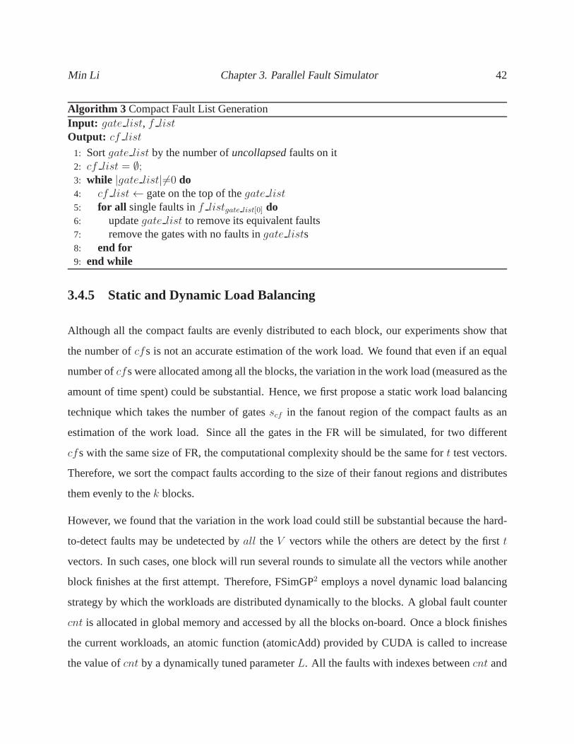
Min Li Chapter 3. Parallel Fault Simulator 42
Algorithm 3 Compact Fault List GenerationInput: gate list, f listOutput: cf list
1: Sortgate list by the number ofuncollapsedfaults on it2: cf list = ∅;3: while |gate list|6=0 do4: cf list← gate on the top of thegate list5: for all single faults inf listgate list[0] do6: updategate list to remove its equivalent faults7: remove the gates with no faults ingate lists8: end for9: end while
3.4.5 Static and Dynamic Load Balancing
Although all the compact faults are evenly distributed to each block, our experiments show that
the number ofcfs is not an accurate estimation of the work load. We found thateven if an equal
number ofcfs were allocated among all the blocks, the variation in the work load (measured as the
amount of time spent) could be substantial. Hence, we first propose a static work load balancing
technique which takes the number of gatesscf in the fanout region of the compact faults as an
estimation of the work load. Since all the gates in the FR willbe simulated, for two different
cfs with the same size of FR, the computational complexity should be the same fort test vectors.
Therefore, we sort the compact faults according to the size of their fanout regions and distributes
them evenly to thek blocks.
However, we found that the variation in the work load could still be substantial because the hard-
to-detect faults may be undetected byall theV vectors while the others are detect by the firstt
vectors. In such cases, one block will run several rounds to simulate all the vectors while another
block finishes at the first attempt. Therefore, FSimGP2 employs a novel dynamic load balancing
strategy by which the workloads are distributed dynamically to the blocks. A global fault counter
cnt is allocated in global memory and accessed by all the blocks on-board. Once a block finishes
the current workloads, an atomic function (atomicAdd) provided by CUDA is called to increase
the value ofcnt by a dynamically tuned parameterL. All the faults with indexes betweencnt and
Min Li Chapter 3. Parallel Fault Simulator 43
cnt + L will be distributed to the blocks for simulation. The operation is atomic in the sense that
it is guaranteed to be performed without interference from other blocks.
Initially, all the blocks will be assignedI compact faults to simulate. Once a block finishes the
simulation of its assigned faults, it will claim anotherL cfs and atomically addL to cnt. A
smallL may diminish the performance because the atomic writing is an expensive operation on
GPU. Also, a bigL may cause an unbalanced work loading if the assignedL FPs are all hard-to-
diagnose. Therefore, we propose a dynamic load balancing strategy where the assignment ofL is
dynamically tuned according to the number of remainingcfs to be simulated. We set a threshold
before which a largeL is selected to avoid too many expensive atomic operations, and we setL
to be1 for the cases where fewcfs remain so that any workload imbalance is minimized during
the final stages of the simulation. Our experimental resultsshow that with such a dynamic load
balancing algorithm, FSimGP2 achieves nearly 2× speed-up against the static load balancing and
4× against the case without load balancing.
3.4.6 Memory Usage and Scalability
Since optimized data access is very important to GPU performance, shared memory is used to store
thedet array which indicates the detection status of faults and thegate data which represents part
of the gates in FRcf . For each block, thedet array only holdst flag entries so that it can fully fit
into the 16 KB shared memory. Only part of thegate information is stored to prevent memory
overflow. With such a setup, the low-latency accesses to shared memory is exploited to accelerate
the frequent read/write operations on these two arrays. Allthe other data stored on the global
memory of the GPU are accessed under a fully coalesced mechanism because all the threads in
a warp always access the same relative addresses on the GPU. For example, thetval of a gate is
stored in a linear array of sizeV corresponding to the number of vectors. Thus, when32 threads
in a warp evaluate the gate,32 consecutive entries intval are coalescedly accessed.
Although our graphic card is equipped with 1 GB device memory, for extremely large circuits,
Min Li Chapter 3. Parallel Fault Simulator 44
such amount of memory may still be insufficient for FSimGP2. Experimental results show that
the storage requirements are mainly occupied by the fault-free and faulty values of internal gates
over allV test vectors whose memory consumptions are calculated by:Mem(tval) = V × G ÷
w, Mem(fval) = k × t × sfr, whereV denotes for the number of vectors,w is the word size
andG is the total number of gates,k andt are the block and pattern- parallelism factors, andsfr
represents the common fanout region size for all the compactfaults. Ideallysfr equals tomax(scf )
which is the maximum fanout region size for allcfs. It is noted thatscf represents the number of
gates in the fanout region of compact faultcf . Next, two cases of memory shortage are analyzed,
and we give a solution for each case:
1. Case 1.Mem(fval) consumes too much memory due tomax(scf ). In such case, we set a
fanout region boundS instead of usingmax(scf ) and divide the faults into two groups. The
faults in group 1 with anscf smaller thanS will be simulated by original strategy. For those
in group 2 with larger FRs, we set a lower pattern parallelismfactort2 so that one block can
simulate the targetcf with fewer threads and thus results in less memory usage. It is noted
that such a solution will not influence the performance when the number of faults in group 2
is few. Otherwise, case 2 should be taken.
2. Case 2.Mem(tval) uses up too much memory, leaving insufficient memory forMem(fval).
In this case, the set ofV vectors is divided intoP partitions, and thus the simulation is di-
vided into several passes between the host and the device. Moreover, we could also decrease
either the block- or pattern- parallelism factor (k/t) to further shrinkMem(fval). Although
the parallelism factors are reduced, our results still demonstrate a huge speedup for both
cases.
3.5 Experimental Results
We evaluated FSimGP2’s performance on a set of large ISCAS89 [15] and ITC99 [27] benchmark
designs which are available from [44]. Our fault simulationplatform consists of a workstation
Min Li Chapter 3. Parallel Fault Simulator 45
with Intel Xeon 3 GHz CPU, 2 Gb memory and one NVIDIA GeForce GTX 285 graphic card as
introduced in Section 2.1.1. We fault simulated 10 sets of 32,768 randomly generated vectors for
all circuits. Ten runs were performed to obtain an average run time because the runtime may be
slightly affected due to the different set of random patterns used in the experiments. To evaluate
the correctness of FSimGP2, the fault simulation results were verified with an open-sourced se-
quential fault simulator, FSIM [51]. The number of blocks (k) launched was set to240 with 64
threads (t) running on each block. As discussed in Section 3.5.2, theseparameters are determined
according to the characteristics of the GPU and CUDA architecture for FSimGP2 to achieve the
best performance. First, we compared the performance of FSimGP2 to those obtained in another
GPU-based fault simulator and a commercial tool from [38]. Next, we compared FSimGP2 to a
recently proposed GPU-based simulator [47], a sequential event-based PPSFP algorithm imple-
mented in [51] and a sequential (non-parallel) version of FSimGP2 to determine the speedup of
FSimGP2. As noted from [47], the FSIM implemented in [51] achieves better performance com-
pared to the simulators in [38].
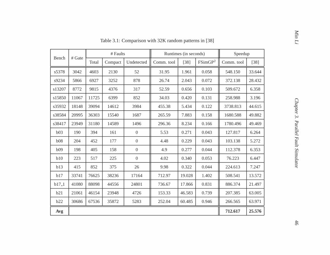
Min
LiC
hapter3.
ParallelF
aultSim
ulator4
6
Table 3.1: Comparison with 32K random patterns in [38]
Bench # Gate# Faults Runtimes (in seconds) Speedup
Total Compact Undetected Comm. tool [38] FSimGP2 Comm. tool [38]
s5378 3042 4603 2130 52 31.95 1.961 0.058 548.150 33.644
s9234 5866 6927 3252 878 26.74 2.043 0.072 372.138 28.432
s13207 8772 9815 4376 317 52.59 0.656 0.103 509.672 6.358
s15850 11067 11725 6399 852 34.03 0.420 0.131 258.988 3.196
s35932 18148 39094 14612 3984 455.38 5.434 0.122 3738.813 44.615
s38584 20995 36303 15540 1687 265.59 7.883 0.158 1680.588 49.882
s38417 23949 31180 14589 1496 296.36 8.234 0.166 1780.496 49.469
b03 190 394 161 0 5.53 0.271 0.043 127.817 6.264
b08 204 452 177 0 4.48 0.229 0.043 103.138 5.272
b09 198 405 158 0 4.9 0.277 0.044 112.378 6.353
b10 223 517 225 0 4.02 0.340 0.053 76.223 6.447
b13 415 852 375 26 9.98 0.322 0.044 224.613 7.247
b17 33741 76625 38236 17164 712.97 19.028 1.402 508.541 13.572
b17 1 41080 88098 44556 24801 736.67 17.866 0.831 886.374 21.497
b21 21061 46154 23948 4726 153.33 46.583 0.739 207.385 63.005
b22 30686 67536 35872 5283 252.04 60.485 0.946 266.565 63.971
Avg 712.617 25.576
Min Li Chapter 3. Parallel Fault Simulator 47
3.5.1 Performance Evaluation
Table 3.1 compared FSimGP2 with a commercial tool reported from [38] and a GPU-based fault
simulator also from [38]. Column 1 lists the name of the benchmark. Benchmarks with∗ are
those with scalability applied (eg., partitioning the testset). The number of gates (NG) and the
number of collapsed faults (Nf ) are listed in columns 2 and 3, respectively. Column 4 lists the
number of compact faults (Ncf ) that groups the gates sharing the same fanout region. We find
thatNcf is approximately equal to half ofNf . Thus the estimated cf-parallelism factor is around
2 which means that the cf-parallelism technique alone couldmake FSimGP2 approximately two
times faster. This estimation of speedup from cf-parallelism is demonstrated in Section 3.5.2.
Column 5 gives the number of undetected faults after applying 32K random vectors. It is noted
that some of those faults may not be undetectable, just that they were not detected by any of the
vectors in the test set. Columns 6 and 7 list the execution time reported in [38]. The former one is a
commercial state-of-the-art fault simulation tool running on a 1.5 GHz UltraSPARC-IV+ processor
with 1.6 GB of RAM while the latter tool is implemented on NVIDIA GeForce GTX 8800 which
has 128 processing cores clocked at 1350 MHz. The on-chip memory contains 768 MB global
memory with 86.4 GB/s bandwidth. We note that our experimental platform is slightly more
advanced than the one used in [38]. The time obtained from FSimGP2 is listed under column 8
which includes all the GPU computation time, the communication overhead between the host and
the device and the GPU data initialization run on the CPU. Thespeedups obtained by FSimGP2
against the sequential commercial tool and GPU-based faultsimulator are listed under columns 9
and 10, respectively. For example, consider circuit s38584, which has more than 20K gates and
36K collapsed faults. With cf-parallelism, these faults are grouped into only 16K compact faults.
1687 of the original collapsed faults were not detected by the 32K vectors. The commercial fault
simulation tool reported from [38] took 265.59 seconds, while the the GPU-based tool proposed
in [38] took 7.883 seconds. Next, our FSimGP2 took only 0.158 seconds. This is 1680× speedup
over the commercial tool and 49× speedup over the GPU-based fault simulator in [38].
An average speed-up of 25.57× is achieved compared to the GPU-based tool [38]. If we consider
Min Li Chapter 3. Parallel Fault Simulator 48
the difference brought about by the new NVIDIA platform, we can conservatively estimate that at
least a 10× speed-up is still achieved. It is noted that the benchmarks used in [38] were optimized
before-hand while our circuits are obtained directly from the benchmark website without any mod-
ifications. Therefore, we believe that the lowest speedup reported for benchmark s15850 is due to
the different netlists used. For example, the s15850 circuit used in [38] had only984 gates while
ours has11067 gates.
To further examine the speedup of FSimGP2, we implemented a sequential version of FSimGP2
called FSimGP2seq. In addition, we compared the results with another non-parallel simulator,
FSIM [51] and a state-of-the-art GPU based simulator proposed in [47]. The results are reported
in Table 3.2. The first five columns are the same as in Table 3.1.Next, the execution time and the
speedup of FSimGP2 over FSimGP2seq are reported in columns 6 and 10, respectively. Likewise,
the results for FSIM [51] and [47] are given in columns 7-8 and11-12. Both sequential tools are
executed on the same workstation which is also used by FSimGP2. It is noted that the results from
[47] are also based on the same platform as ours. We cannot compare all the result against with
[47] because some industrial benchmarks in [47] are not openly available. Using the circuit b171
as an example, [47] took 3.89 seconds to complete while FSimGP2seq and FSIM [51] took 539.018
and 79.283 seconds, respectively. Our FSimGP2 took 0.831 seconds. This is about 4× speedup
over [47] and 95×, 648× speedup over the sequential version of FSimGP2 and FSIM, respectively.
Note that FSIM was able to complete the simulation in a much shorter time than the commercial
tool reported in Table 3.1. Such a difference could be due to the platform difference between them.
For circuit s13207, FSimGP2 has the smallest speedup against the other tools. This is because
the percentage of undetected faults (317 out of 9815) is so low that the number of computations
needed for fault simulation is reduced greatly. In other words, most faults in s13207 were easy to
be detected. This could also explain the highest speedup gained for circuit b171 since there are
more than 25% undetected faults and thus the simulation requires more computational efforts.
In Table 3.3, the break up of runtime for various steps duringsimulation is reported in seconds.
The total runtime is listed in column 2 (Total). The cost of GPU data initialization process is
Min Li Chapter 3. Parallel Fault Simulator 49
listed in column 3 (Init.). Since most of the time taken in this process is to allocate memory space
on the GPU, the runtime is similar among the benchmarks. The simulation kernel to compute
the fault-free value is listed in column 3 (Sim.). Column 4 (Fsim.) denotes the runtime for fault
simulation kernel which takes most of the runtime for some large benchmarks. The transmission
overhead between the CPU and the GPU is presented in column 5 (Tran.). As illustrated in 3.4.2,
the communication costs only includes the circuit data and test vectors sent from CPU and the
faults detection results from GPU. Therefore, the overheadis relatively small comparing with the
total runtime. It is noted that the total runtime might be larger than the sum of the four steps’
runtime due to the overhead of timing function in use.
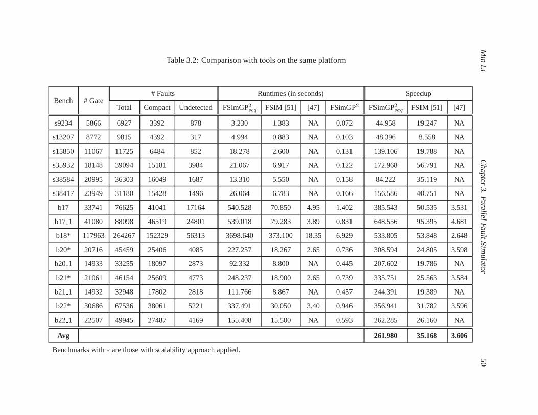
Min
LiC
hapter3.
ParallelF
aultSim
ulator5
0Table 3.2: Comparison with tools on the same platform
Bench # Gate# Faults Runtimes (in seconds) Speedup
Total Compact Undetected FSimGP2seq FSIM [51] [47] FSimGP2 FSimGP2seq FSIM [51] [47]
s9234 5866 6927 3392 878 3.230 1.383 NA 0.072 44.958 19.247 NA
s13207 8772 9815 4392 317 4.994 0.883 NA 0.103 48.396 8.558 NA
s15850 11067 11725 6484 852 18.278 2.600 NA 0.131 139.106 19.788 NA
s35932 18148 39094 15181 3984 21.067 6.917 NA 0.122 172.968 56.791 NA
s38584 20995 36303 16049 1687 13.310 5.550 NA 0.158 84.222 35.119 NA
s38417 23949 31180 15428 1496 26.064 6.783 NA 0.166 156.586 40.751 NA
b17 33741 76625 41041 17164 540.528 70.850 4.95 1.402 385.543 50.535 3.531
b17 1 41080 88098 46519 24801 539.018 79.283 3.89 0.831 648.556 95.395 4.681
b18* 117963 264267 152329 56313 3698.640 373.100 18.35 6.929 533.805 53.848 2.648
b20* 20716 45459 25406 4085 227.257 18.267 2.65 0.736 308.594 24.805 3.598
b20 1 14933 33255 18097 2873 92.332 8.800 NA 0.445 207.602 19.786 NA
b21* 21061 46154 25609 4773 248.237 18.900 2.65 0.739 335.751 25.563 3.584
b21 1 14932 32948 17802 2818 111.766 8.867 NA 0.457 244.391 19.389 NA
b22* 30686 67536 38061 5221 337.491 30.050 3.40 0.946 356.941 31.782 3.596
b22 1 22507 49945 27487 4169 155.408 15.500 NA 0.593 262.285 26.160 NA
Avg 261.980 35.168 3.606
Benchmarks with∗ are those with scalability approach applied.
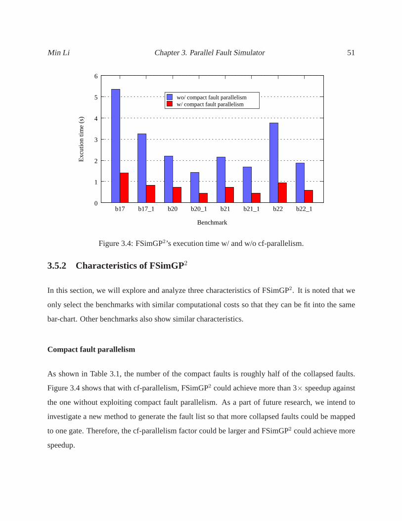
Min Li Chapter 3. Parallel Fault Simulator 51
0
1
2
3
4
5
6
b17 b17_1 b20 b20_1 b21 b21_1 b22 b22_1
Exc
utio
n tim
e (s
)
Benchmark
wo/ compact fault parallelismw/ compact fault parallelism
Figure 3.4: FSimGP2’s execution time w/ and w/o cf-parallelism.
3.5.2 Characteristics of FSimGP2
In this section, we will explore and analyze three characteristics of FSimGP2. It is noted that we
only select the benchmarks with similar computational costs so that they can be fit into the same
bar-chart. Other benchmarks also show similar characteristics.
Compact fault parallelism
As shown in Table 3.1, the number of the compact faults is roughly half of the collapsed faults.
Figure 3.4 shows that with cf-parallelism, FSimGP2 could achieve more than 3× speedup against
the one without exploiting compact fault parallelism. As a part of future research, we intend to
investigate a new method to generate the fault list so that more collapsed faults could be mapped
to one gate. Therefore, the cf-parallelism factor could be larger and FSimGP2 could achieve more
speedup.
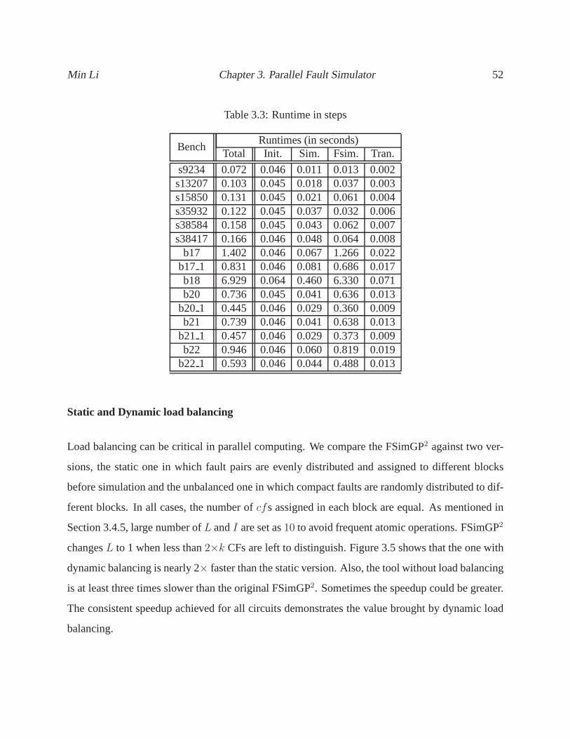
Min Li Chapter 3. Parallel Fault Simulator 52
Table 3.3: Runtime in steps
BenchRuntimes (in seconds)
Total Init. Sim. Fsim. Tran.
s9234 0.072 0.046 0.011 0.013 0.002s13207 0.103 0.045 0.018 0.037 0.003s15850 0.131 0.045 0.021 0.061 0.004s35932 0.122 0.045 0.037 0.032 0.006s38584 0.158 0.045 0.043 0.062 0.007s38417 0.166 0.046 0.048 0.064 0.008
b17 1.402 0.046 0.067 1.266 0.022b17 1 0.831 0.046 0.081 0.686 0.017b18 6.929 0.064 0.460 6.330 0.071b20 0.736 0.045 0.041 0.636 0.013
b20 1 0.445 0.046 0.029 0.360 0.009b21 0.739 0.046 0.041 0.638 0.013
b21 1 0.457 0.046 0.029 0.373 0.009b22 0.946 0.046 0.060 0.819 0.019
b22 1 0.593 0.046 0.044 0.488 0.013
Static and Dynamic load balancing
Load balancing can be critical in parallel computing. We compare the FSimGP2 against two ver-
sions, the static one in which fault pairs are evenly distributed and assigned to different blocks
before simulation and the unbalanced one in which compact faults are randomly distributed to dif-
ferent blocks. In all cases, the number ofcfs assigned in each block are equal. As mentioned in
Section 3.4.5, large number ofL andI are set as10 to avoid frequent atomic operations. FSimGP2
changesL to 1 when less than2×k CFs are left to distinguish. Figure 3.5 shows that the one with
dynamic balancing is nearly 2× faster than the static version. Also, the tool without load balancing
is at least three times slower than the original FSimGP2. Sometimes the speedup could be greater.
The consistent speedup achieved for all circuits demonstrates the value brought by dynamic load
balancing.
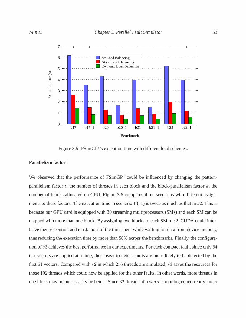
Min Li Chapter 3. Parallel Fault Simulator 53
0
1
2
3
4
5
6
7
b17 b17_1 b20 b20_1 b21 b21_1 b22 b22_1
Exc
utio
n tim
e (s
)
Benchmark
w/ Load BalancingStatic Load BalancingDynamic Load Balancing
Figure 3.5: FSimGP2’s execution time with different load schemes.
Parallelism factor
We observed that the performance of FSimGP2 could be influenced by changing the pattern-
parallelism factort, the number of threads in each block and the block-parallelism factork, the
number of blocks allocated on GPU. Figure 3.6 compares threescenarios with different assign-
ments to these factors. The execution time in scenario 1 (s1) is twice as much as that ins2. This is
because our GPU card is equipped with 30 streaming multiprocessors (SMs) and each SM can be
mapped with more than one block. By assigning two blocks to each SM ins2, CUDA could inter-
leave their execution and mask most of the time spent while waiting for data from device memory,
thus reducing the execution time by more than 50% across the benchmarks. Finally, the configura-
tion of s3 achieves the best performance in our experiments. For each compact fault, since only64
test vectors are applied at a time, those easy-to-detect faults are more likely to be detected by the
first 64 vectors. Compared withs2 in which 256 threads are simulated,s3 saves the resources for
those192 threads which could now be applied for the other faults. In other words, more threads in
one block may not necessarily be better. Since32 threads of awarp is running concurrently under
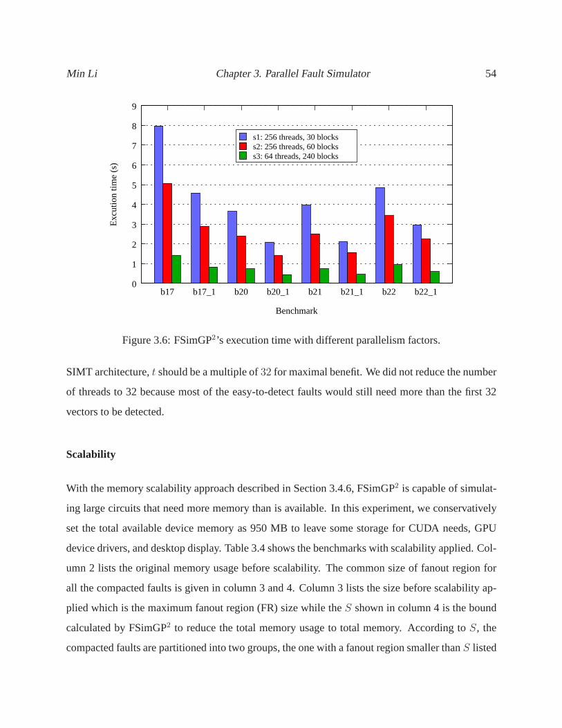
Min Li Chapter 3. Parallel Fault Simulator 54
0
1
2
3
4
5
6
7
8
9
b17 b17_1 b20 b20_1 b21 b21_1 b22 b22_1
Exc
utio
n tim
e (s
)
Benchmark
s1: 256 threads, 30 blockss2: 256 threads, 60 blockss3: 64 threads, 240 blocks
Figure 3.6: FSimGP2’s execution time with different parallelism factors.
SIMT architecture,t should be a multiple of32 for maximal benefit. We did not reduce the number
of threads to 32 because most of the easy-to-detect faults would still need more than the first 32
vectors to be detected.
Scalability
With the memory scalability approach described in Section 3.4.6, FSimGP2 is capable of simulat-
ing large circuits that need more memory than is available. In this experiment, we conservatively
set the total available device memory as 950 MB to leave some storage for CUDA needs, GPU
device drivers, and desktop display. Table 3.4 shows the benchmarks with scalability applied. Col-
umn 2 lists the original memory usage before scalability. The common size of fanout region for
all the compacted faults is given in column 3 and 4. Column 3 lists the size before scalability ap-
plied which is the maximum fanout region (FR) size while theS shown in column 4 is the bound
calculated by FSimGP2 to reduce the total memory usage to total memory. According to S, the
compacted faults are partitioned into two groups, the one with a fanout region smaller thanS listed
Min Li Chapter 3. Parallel Fault Simulator 55
in column 5, and the one with biggerscf listed in column 6.
As an example, the memory usage of benchmark b22 before scaling is 1.38 GB which exceeds
950 MB. After we set the fanout region boundS to be 11841 instead of the originalmax(scf ) of
18936, the total memory consumption reduced to 949 MB which can fit into total memory. Also,
only 48 compacted faults have a large fanout region and need to be simulated by fewer threads
(t2 = 32) concurrently. Another benchmark b18 falls into case 2 as discussed in Section 3.4.6
with an original memory usage of 1.9 GB. We partitioned the input vectors into two (P = 2) parts,
reduced the cf-parallelism factork to 120 (originalk is 240) and set the FR boundS to be 12180
(max(scf ) is 17033). Consequently, the total memory usage is reduced to 949 MB.
We note that that the performance should be affected by the scalability approach. However, in both
two cases, FSimGP2 achieves 31.782× and 53.848× speedup over FSIM [1]. We investigated the
impact of scalability approach case by case. In case 1, although the pattern parallelism factort is
reduced from64 to 32, the performance was not affected much as long as all the threads within
one warp ran together. Moreover, the number of faults with a large size of fanout region,scf is
limited. For example, only 48 compacted faults in benchmarkb 22 need to be simulated with a
smallt instead of the original 35872 faults.
Case 2 introduces the communication overhead between the host and the device among several
passes of simulation. However, our experimental results show that for benchmark b18, the over-
head between the simulation of two partitioned inputs is only 0.01154 seconds which is relatively
small compared with the simulation process. Table 3.3 showsthat for all circuits, the total trans-
mission cost is small.
We estimated that the1 GB device memory is insufficient to store large size of fanout region
(scf ) with more than one million gates. The reason is that the circuit netlist, true and faulty logic
values have to be stored on-board to achieve high bandwidth throughput. However, it is noted that
with the recently announced Tesla GPU server s2070 [73] housing up to 24 GB GDDR5 device
memory, we can simulate even larger benchmark before we needto apply the scalability methods.
Moreover, as a future work, the simulation based on stem region in [47] may help to further reduce
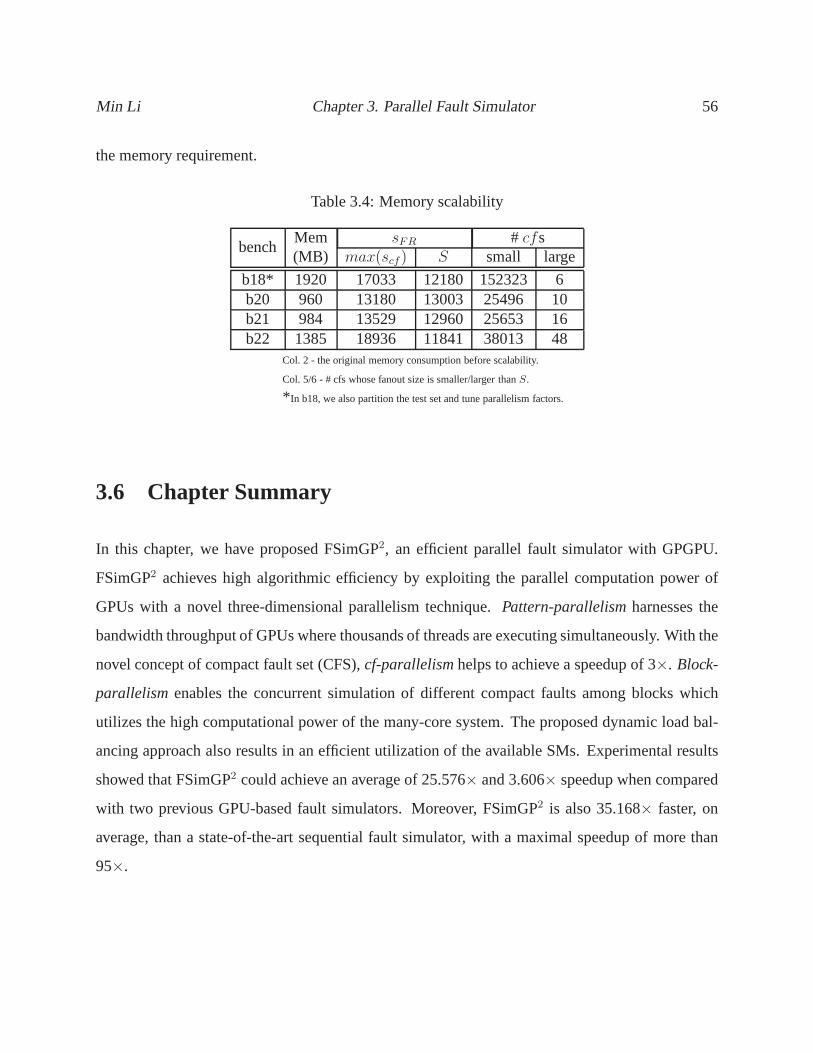
Min Li Chapter 3. Parallel Fault Simulator 56
the memory requirement.
Table 3.4: Memory scalability
benchMem sFR # cfs(MB) max(scf) S small large
b18* 1920 17033 12180 152323 6b20 960 13180 13003 25496 10b21 984 13529 12960 25653 16b22 1385 18936 11841 38013 48
Col. 2 - the original memory consumption before scalability.
Col. 5/6 - # cfs whose fanout size is smaller/larger thanS.
* In b18, we also partition the test set and tune parallelism factors.
3.6 Chapter Summary
In this chapter, we have proposed FSimGP2, an efficient parallel fault simulator with GPGPU.
FSimGP2 achieves high algorithmic efficiency by exploiting the parallel computation power of
GPUs with a novel three-dimensional parallelism technique. Pattern-parallelismharnesses the
bandwidth throughput of GPUs where thousands of threads areexecuting simultaneously. With the
novel concept of compact fault set (CFS),cf-parallelismhelps to achieve a speedup of 3×. Block-
parallelismenables the concurrent simulation of different compact faults among blocks which
utilizes the high computational power of the many-core system. The proposed dynamic load bal-
ancing approach also results in an efficient utilization of the available SMs. Experimental results
showed that FSimGP2 could achieve an average of 25.576× and 3.606× speedup when compared
with two previous GPU-based fault simulators. Moreover, FSimGP2 is also 35.168× faster, on
average, than a state-of-the-art sequential fault simulator, with a maximal speedup of more than
95×.
Chapter 4
Parallel Diagnostic Fault Simulator
4.1 Chapter Overview
In this chapter, we present an efficient diagnostic fault simulator based on a state-of-the-art graphic
processing unit. Diagnostic fault simulation plays an important role to identify and locate the
causes of circuit failures. However, today’s complex VLSI circuits pose ever higher computational
demand for such simulators. Our GPU based diagnostic fault simulator (GDSim) is based on a
novel two-stage simulation framework which exploits high computation efficiency on the GPU.
The fault pair based simulation is proposed to overcome the limited capacity of GPU memory
as well as achieve a substantial fine-grained parallelism. Multi-fault-signature and dynamic load
balancing techniques are introduced for the best usage of computing resources on-board. Experi-
mental results demonstrate a speedup of up to 121× (with average speedup of 38.43×) compared
to a state-of-the-art CPU-based diagnostic fault simulator.
The rest of the chapter is organized as follows. A brief introduction is given in Section 4.2. In
Section 4.3, we review the previous work related with diagnostic fault simulation. Section 4.4
outlines a high-level process view of the proposed method, with a detail description of some critical
approaches. The experimental results are reported in Section 4.5. Finally Section 4.6 concludes
57
Min Li Chapter 4. Parallel Diagnostic Fault Simulator 58
the chapter.
4.2 Introduction
Fault diagnosis, a process of locating defects in a defective chip, plays an important role in today’s
very-large-scale integrated (VLSI) circuits. The manufacturing defects are becoming more subtle
due to rapidly diminishing feature sizes and complex fabrication processes. To improve yield,
such defects could be identified and located using fault diagnosis followed by rectification with
visual inspection or electron-beam probing. For a circuit-under-diagnosis (CUD) in the presence
of modeled faults, the process of evaluating diagnostic capability of the givenN test patterns
is called diagnostic fault simulation. In addition to measuring diagnostic capability, diagnostic
simulators can also help to accelerate automated diagnostic pattern generation (ADPG).
In the past, significant efforts have been devoted to accelerate this process [19, 23, 82]. While fault
simulation could already be expensive on industry-sized circuits, diagnostic fault simulation can
often cost one to two orders of magnitude higher. Furthermore, the computational requirements
increase significantly with the increasing size of the circuit (hence increasing number of fault
pairs). Therefore, there is a need for efficient diagnostic fault simulators that are able to handle
large designs with extremely large test sets.
In this chapter, we present a fine-grained GPU-based diagnostic fault simulator (GDSim). The
main motivation is to harness the computational power of GPUs to reduce the total execution time
without compromising the output fidelity. Experimental results show that GDSim achieves one
to two orders of magnitude speedup in comparison with a state-of-the-art CPU-based diagnostic
fault simulator and a sequential version of the GPU-based implementation. We summarize our
contributions as follows.
• To the best of our knowledge, this work is the first that accelerates diagnostic fault simulation
on a GPU platform.
Min Li Chapter 4. Parallel Diagnostic Fault Simulator 59
• We introduce a two-stage simulation framework to efficiently utilize the computation power
of the GPU without exceeding its memory limitation. First, afault simulation kernel (ksim)
is launched to determine the detectability of each fault. Then the detected faults are dis-
tinguished by the fault pair based diagnostic simulation kernel (kdiag). Both kernels are
parallelized on the GPU architecture.
• In theksim kernel,multi-fault-signature(MFS) is proposed to facilitate fault pair list gen-
eration. MFSs can be obtained directly from the parallel fault simulation without intro-
ducing any computational overhead on GPUs. By clever selection of the size of the MFS
(SIG LEN), GDSim is able to reduce the number of fault pairs by 66%.
• The fault pair based diagnostic simulation kernel,kdist, exploits both fault pair- and pattern-
parallelism, which allows for efficient utilization of memory bandwidth and massive data
parallelism on GPUs.
• In kdist, dynamic load balancing is introduced to guarantee an even workload onto each
processing elements.
• We applied GPU-oriented performance optimization strategies on GDSim to ensure a max-
imal speedup. Global memory accesses are coalesced to achieve maximum memory band-
width. The maximum instruction bandwidth is obtained by avoiding branch divergence.
GDSim also takes advantage of the inherent bit-parallelismof logic operations on computer
words.
4.3 Background
4.3.1 Diagnostic Fault Simulation
A diagnostic fault simulator computes the diagnostic capability of the given test vectors. Our pro-
posed approach targets on full-scan gate-level circuits and assumes the single stuck-at fault model.
Min Li Chapter 4. Parallel Diagnostic Fault Simulator 60
Given a large set of random vectors, our GDSim is to obtain andrecord all the indistinguishable
fault pairs from a collapsed fault list.
The diagnostic capability could be evaluated by several measures such asdiagnostic resolution
(DR), the fraction of fault pairs distinguished [17], anddiagnostic power (DP), the fraction of
fully distinguishable faults [17]. Here, two faultsf andg in a combinational circuit are said to be
distinguishableif, for at least one input vector, the responses of corresponding circuits are different
on at least one primary output (PO). To provide a more accurate diagnostic information, the authors
in [50] have proposed a third measure,Equivalence Class (EC)which identifies sets of equivalent
faults under given test patterns for a circuit. Sinceall the indistinguishable fault pairs are recorded
by our GPU-based simulator, EC could be computed in linear time. Also, the measures, DP and
DR, can be computed from the sizes of indistinguishable classes in EC. Therefore, GDSim is
capable of providing all the above diagnostic measures.
4.3.2 Previous Work
In [19], an algorithm called “multiway list splitting” for computing EC (of stuck-at faults) is pre-
sented. Initially the EC is a class including all the faults.For each test vector, all the faults are
simulated and their corresponding outputs are recorded. Hence, the faults with the same output
vectors are grouped into the same set which divides the original EC into several smaller subsets.
The EC is obtained when all the vectors have been simulated. The authors in [23] proposed a
distributed approach to get the indistinguishable fault list (IFL) that stores the faults which are
indistinguishable from each fault. All the machines run a similar fault simulator to maintain the
IFL. Although significant speedups are achieved for both methods mentioned above, they are not
applicable to the CUDA architecture due to the expensive global synchronization between blocks
as well as the infeasible operations of dynamic list. Finally, since thousands of test vectors are sim-
ulated concurrently on GPUs, the storage of the corresponding output vectors for a large number of
faults within the same set will cause memory explosion on theGPU. To overcome this, our GDSim
targets at fault pairs where each thread block simulates andcomparesonly two faults concurrently.
Min Li Chapter 4. Parallel Diagnostic Fault Simulator 61
The fault pairs are generated based on indistinguishable fault sets obtained from the initial parallel
fault simulation on the GPU (ksim). Such a strategy takes advantage of the GPU’s large memory
bandwidth and high computational power while avoids the memory limitation on-board.
A fault table generation on GPUs is proposed in [39] which maybe used for fault diagnosis.
The fault simulation algorithm based on the parallel-pattern single-fault propagation (PPSFP) is
mapped to the CUDA architecture. Although the fault table could be used to differentiate faults,
it is unnecessary to simulateall the test vectors because the complete fault table is an overkill to
evaluate diagnostic measures such as EC. Moreover, only those vectors that detect the faults are
recorded in [39]. Such information without the exact corresponding output vectors is insufficient
to fully distinguish two faults.
4.4 Proposed Method
In this section, we first present some definitions, followed by the two-stage framework of the
proposed diagnostic fault simulator and the dynamic load balancing technique.
Definition 9. The gate on which a set of faults are located is defined asfaulty gate(FG). For the
group of faults on the same gate, only the gates in the fanout region (FR) beyond FG need to be
evaluated during fault simulation. The set of gates in the fanout region is termed as FRFG.
Definition 10. The fault signature(FSIG) for a faultf is defined as a pair fsigf (v,p), where the
faults are excited by the vth vector and its faulty value is propagated to the pth PO of the circuit.
Since the faulty value may be propagated to several POs of thecircuit and detected by multiple
vectors, we define amultiple-fault-signatureset for a faultf as MFSf (k) which records thefirst k
FSIGs. The FSIGs detected by the same vector but at differentPOs are sorted byp, the indices of
POs.
Definition 11. Two faultsf1 andf2 with the same size of MFS: MFSf1(k), MFSf2(k), are distin-
guished if at least one of the corresponding FSIGs differ.
Min Li Chapter 4. Parallel Diagnostic Fault Simulator 62
Assume that theith FSIG, fsigf1(v1,p1) and fsigf2(v2,p2), differ while the firsti − 1 components
of the MFSs are the same. Case 1,v1 6=v2. Without loss of generality, assumingv1 < v2, we know
thatf1 is detected by vectorv1 while f2 is not. Thus the fault pair could be distinguished byv1.
Case 2,v1 = v2, p1 6=p2. Assumep1 < p2 without loss of generality. Because all the firsti − 1
FSIGs are the same for both faults and they are sorted with respect to the PO indices,f2 cannot be
detected at POp1 by vectorv1. Hence, these two faults are distinguishable byv1 at POp1.
4.4.1 Framework
The high-level flow of GDSim is shown in Figure 4.1. At the beginning, the CPU reads in the
circuit netlist and generates its collapsed fault list. Thelist of faults will be grouped with respect to
their locations. For the faults on the same gate, its fanout region (FRFG) is processed by a breadth-
first search from the faulty gate location in a forward levelized manner. Then, the test vectors and
all the fundamental data, including circuit netlist, fault list with correspondingFRFG, and input
vectors, will be transferred to the GPU. A GPU-based fault simulatorksim is launched as Kernel 1
on the GPU. It is an extended version of the simulator implemented from [54] with MFSs recorded
which will be used to sort the fault list by Kernel 2. The sorted fault list will be transferred back
to the host and the CPU will generate the list of fault pairs for further analysis. After the GPU
receives the fault pairs to be simulated, the third kernelkdiag is launched. We run the given test
vectors on each fault pair until the two faults are distinguished. If no pattern is able to distinguish
a fault pair, it is also recorded. Finally, the information of the complete list of indistinguishable
fault pairs can be used to obtain diagnostic measures such asEC and/or provide a set potential fault
locations.
Faulty Gate based Parallel Fault Simulation (ksim)
For a faulty gatefg, each gate in FRfg will be fault-simulated witht vectors, processed ont threads
in one block. To inject the fault, we justcomplementthe fault-free value of the faulty gate for all
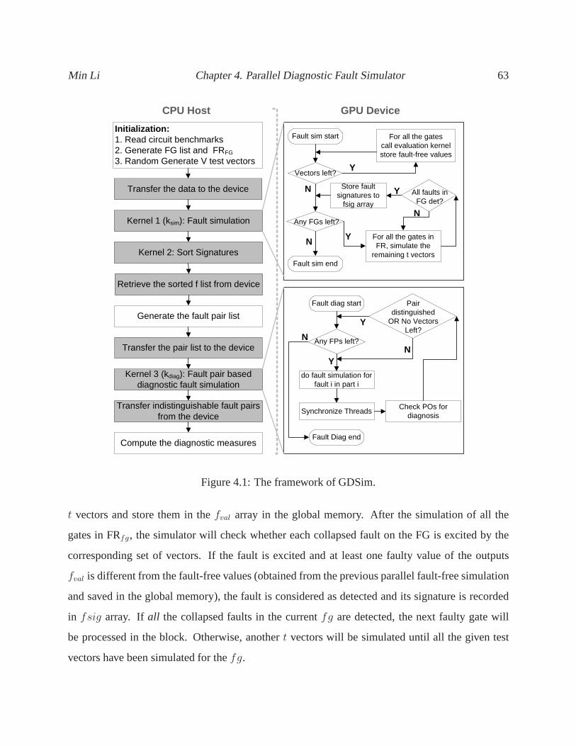
Min Li Chapter 4. Parallel Diagnostic Fault Simulator 63
CPU Host
Initialization:1. Read circuit benchmarks2. Generate FG list and FRFG
3. Random Generate V test vectors
Transfer the data to the device
Kernel 1 (ksim): Fault simulation
Retrieve the sorted f list from device
Generate the fault pair list
Transfer the pair list to the device
Kernel 3 (kdiag): Fault pair based diagnostic fault simulation
Vectors left?
For all the gatescall evaluation kernelstore fault-free values
Fault sim start
For all the gates in FR, simulate the
remaining t vectors
Store fault signatures to
fsig array
Fault sim end
Fault diag start
Any FPs left?
Fault Diag end
do fault simulation for fault i in part i
Check POs for diagnosis
GPU Device
Synchronize ThreadsTransfer indistinguishable fault pairs
from the device
Compute the diagnostic measures
Pair distinguished
OR No Vectors Left?
N Y
Y
N
Y
NN
Y
Kernel 2: Sort Signatures
Any FGs left?
Y
N All faults in FG det?
Figure 4.1: The framework of GDSim.
t vectors and store them in thefval array in the global memory. After the simulation of all the
gates in FRfg, the simulator will check whether each collapsed fault on the FG is excited by the
corresponding set of vectors. If the fault is excited and at least one faulty value of the outputs
fval is different from the fault-free values (obtained from the previous parallel fault-free simulation
and saved in the global memory), the fault is considered as detected and its signature is recorded
in fsig array. If all the collapsed faults in the currentfg are detected, the next faulty gate will
be processed in the block. Otherwise, anothert vectors will be simulated until all the given test
vectors have been simulated for thefg.
Min Li Chapter 4. Parallel Diagnostic Fault Simulator 64
Given the above discussion, our approach simulates a set of faults on the same FG undert vectors
concurrently. The simulator records detection information as the multi-fault signatures. We set
an upper bound of the MFS size as SIGLEN so that the signatures of faultfi includes at most
SIG LEN FSIGs. Such MFS mechanisms will not cause any overhead inour implementation
because we are simulating only for the faults yet to be detected infg. However, it is not the case
in single fault based simulation because more simulations have to be performed to get multiple
signatures for a single fault.
After simulating all the FGs, the simulator will call Kernel2 which is a parallel radix sort program
provided in CUDA software development kit (SDK) [72] to sortthe fault list.
Fault pair based Parallel Diagnostic Fault Simulation (kdiag)
To utilize memory bandwidth and massive data parallelism inan efficient way, our diagnostic fault
simulator exploits bothfault pair- andpattern-parallelism. Namely, we simulate multiple fault
pairs over multiple test patterns at a time. As illustrated in Figure 4.2, theNfp fault pairs (FPs) are
distributed ontok thread blocks running concurrently on the GPU. Each block allocatest threads
simulatingt/2 test vectors for one fault pair in parallel:t/2 threads process faultf1 and the other
t/2 threads process the other faultf2 of the pair. For example,block1 in the figure is assigned with
fpi, which includes two single faults,f1 andf2. The first half of the threads deal withf1 while
f2 is simulated by the rest of the threads. Since32 threads within a warp are running together, the
branch divergence is prevented as long ast/2 is a multiple of32. All the fault pairsdynamically
assigned for one block are processed sequentially.
As we mentioned before, the fault set based simulation in [19] is not applicable here because of the
memory limitation on GPUs. Since a certain fault set may contain more than one hundred faults
and we are simulating thousands of vectors concurrently on the GPU, the storage of all those faulty
signatures on GPUs for comparison can become very large. However, by distinguishing fault pairs
separately, the storage of signatures is no longer needed, and we only need to compute the faulty
value of POs fromfval array. Also, our experiments show that the number of fault pairs to be
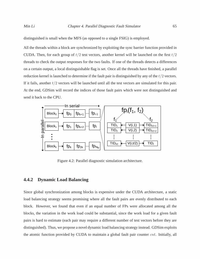
Min Li Chapter 4. Parallel Diagnostic Fault Simulator 65
distinguished is small when the MFS (as opposed to a single FSIG) is employed.
All the threads within a block are synchronized by exploiting the sync barrier function provided in
CUDA. Then, for each group oft/2 test vectors, another kernel will be launched on the firstt/2
threads to check the output responses for the two faults. If one of the threads detects a differences
on a certain output, a local distinguishable flag is set. Onceall the threads have finished, a parallel
reduction kernel is launched to determine if the fault pair is distinguished by any of thet/2 vectors.
If it fails, anothert/2 vectors will be launched until all the test vectors are simulated for this pair.
At the end, GDSim will record the indices of those fault pairswhich were not distinguished and
send it back to the CPU.
In p
aral
lel
Block0 fp0
In serial
fpk+1 fpi-1...
Block1 fp1 fpk+2 fpi...
Blockk fpk fp2k fpN...
...
fp
fpi(f1, f2)f1
...
f2
V(i,t/2)
V(i,1)
V(i,2)
TIDt/2+1
TIDt/2+2
TIDt
TID1
TID2
TIDt/2
... ...
Figure 4.2: Parallel diagnostic simulation architecture.
4.4.2 Dynamic Load Balancing
Since global synchronization among blocks is expensive under the CUDA architecture, a static
load balancing strategy seems promising where all the faultpairs are evenly distributed to each
block. However, we found that even if an equal number of FPs were allocated among all the
blocks, the variation in the work load could be substantial,since the work load for a given fault
pairs is hard to estimate (each pair may require a different number of test vectors before they are
distinguished). Thus, we propose a novel dynamic load balancing strategy instead. GDSim exploits
the atomic function provided by CUDA to maintain a global fault pair countercnt. Initially, all
Min Li Chapter 4. Parallel Diagnostic Fault Simulator 66
the blocks are assignedI fault pairs to distinguish. Once a block finishes the simulation of its
assigned FPs, it will claim anotherL FPs and atomically addL to cnt. A smallL may diminish
the performance because the atomic writing is an expensive operation on GPU. Also, a bigL may
cause an unbalanced work loading if the assignedL FPs are all hard-to-diagnose. Therefore, we
propose a dynamic load balancing strategy whereL is dynamically tuned according to the number
of remaining fps to be simulated. We initially set a largeLb to avoid too many expensive atomic
operations, and later reduceL to 1 for when few FPs remain so that any workload imbalance is
minimized during the final stages of the simulation.
4.5 Experimental Results
We evaluated our diagnostic fault simulator’s performanceon a set of large ISCAS89 [15] and
ITC99 [27] benchmarks. The experimental platform consistsof a workstation with Intel Xeon
3 GHz CPU, 2 GB memory and one NVidia GeForce GTX 285 graphic card as introduced in
Section 2.1.1. We randomly generated 10 sets of 32,768 test vectors and applied them to all
the circuits for diagnostic fault simulation. Ten runs wereperformed to obtain an average run
time. To evaluate the correctness of our simulator, the results were verified with an efficient CPU-
based diagnostic fault simulator [19]. The number of blocks(k) launched was set to120 with 128
threads (t) running on each block. As discussed in Section 4.5.2, theseparameters are determined
according to the characteristics of the GPU and CUDA architecture for GDSim to achieve the best
performance.
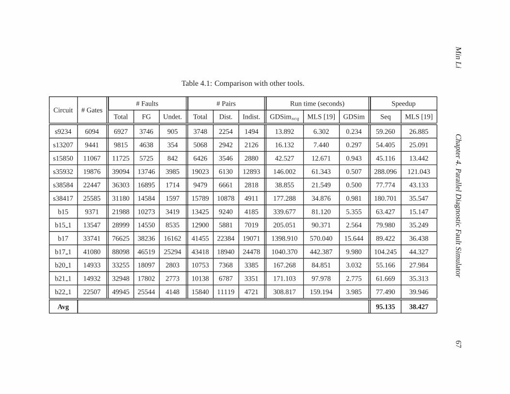
Min
LiC
hapter4.
ParallelD
iagnosticF
aultSim
ulator6
7
Table 4.1: Comparison with other tools.
Circuit # Gates# Faults # Pairs Run time (seconds) Speedup
Total FG Undet. Total Dist. Indist. GDSimseq MLS [19] GDSim Seq MLS [19]
s9234 6094 6927 3746 905 3748 2254 1494 13.892 6.302 0.234 59.260 26.885
s13207 9441 9815 4638 354 5068 2942 2126 16.132 7.440 0.297 54.405 25.091
s15850 11067 11725 5725 842 6426 3546 2880 42.527 12.671 0.943 45.116 13.442
s35932 19876 39094 13746 3985 19023 6130 12893 146.002 61.343 0.507 288.096 121.043
s38584 22447 36303 16895 1714 9479 6661 2818 38.855 21.549 0.500 77.774 43.133
s38417 25585 31180 14584 1597 15789 10878 4911 177.288 34.876 0.981 180.701 35.547
b15 9371 21988 10273 3419 13425 9240 4185 339.677 81.120 5.355 63.427 15.147
b15 1 13547 28999 14550 8535 12900 5881 7019 205.051 90.371 2.564 79.980 35.249
b17 33741 76625 38236 16162 41455 22384 19071 1398.910 570.040 15.644 89.422 36.438
b17 1 41080 88098 46519 25294 43418 18940 24478 1040.370 442.387 9.980 104.245 44.327
b20 1 14933 33255 18097 2803 10753 7368 3385 167.268 84.851 3.032 55.166 27.984
b21 1 14932 32948 17802 2773 10138 6787 3351 171.103 97.978 2.775 61.669 35.313
b22 1 22507 49945 25544 4148 15840 11119 4721 308.817 159.194 3.985 77.490 39.946
Avg 95.135 38.427
Min Li Chapter 4. Parallel Diagnostic Fault Simulator 68
4.5.1 Performance Evaluation
Table 4.1 compares our GPU-based diagnostic fault simulator (GDSim) with its own sequen-
tial (non-parallel) version (GDSimseq) and a ”multi-way list splitting” (MLS) algorithm proposed
from [19]. Both of these two methods are implemented and tested on the same platform as GDSim.
In Table 4.1, Column 1 lists the benchmarks. The number of gates and the number of collapsed
faults are listed in columns 2 and 3, respectively. Column 4 lists the number of faulty gates (NFG);
recall that each FG denotes a group of faults on the same gate.Columns 5 and 6 give the number
of undetected faults and the number of fault pairs, respectively. These fault pairs will be sent to
GPU for further pair-based diagnostic fault simulation. Itis noted that the pairs consisting of two
undetected faults are not included because all those are already identified as indistinguishable by
the test set. The size of MFS (SIGLEN) is limited to 3 in our experiment. SIGLEN are ex-
perimentally determined and will be discussed in Section 4.5.2. After pair-based simulation, the
number of obtained distinguishable (indistinguishable) pairs by the total 32K testing vectors are
presented in Column 7 (8). Columns 9 and 10 list the executiontime in seconds for GDSimseq and
MLS [19], respectively. The time obtained from our parallelsimulator GDSim is listed under col-
umn 11 which includes the GPU computation time, the communication overhead between the host
and the device and the pre-processing tasks run on the CPU. The speedups obtained by GDSim
against these two tools are listed under columns 12 to 13.
Consider circuit s35932, which has more than 20K gates and 39K collapsed faults. With multi-
signatures fault simulation, only19023 fault pairs need to be simulated, among which6130 pairs
were distinguished and12893 pairs indistinguishable by the 32K random vectors. GDSimseq took
146 seconds to complete, while MLS proposed in [19] took61 seconds on the CPU of the setup.
Our GDSim on GPU took only0.51 seconds. This is288×, 121× speedup over these tools,
respectively.
We note that GDSim has the smallest speedup for s15850. This is because of the low percentage of
indistinguishable faults pairs (2880 out of 6426). Therefore, the number of computations needed
for sequential diagnosis simulation is reduced greatly. Inother words, the distinguishability of
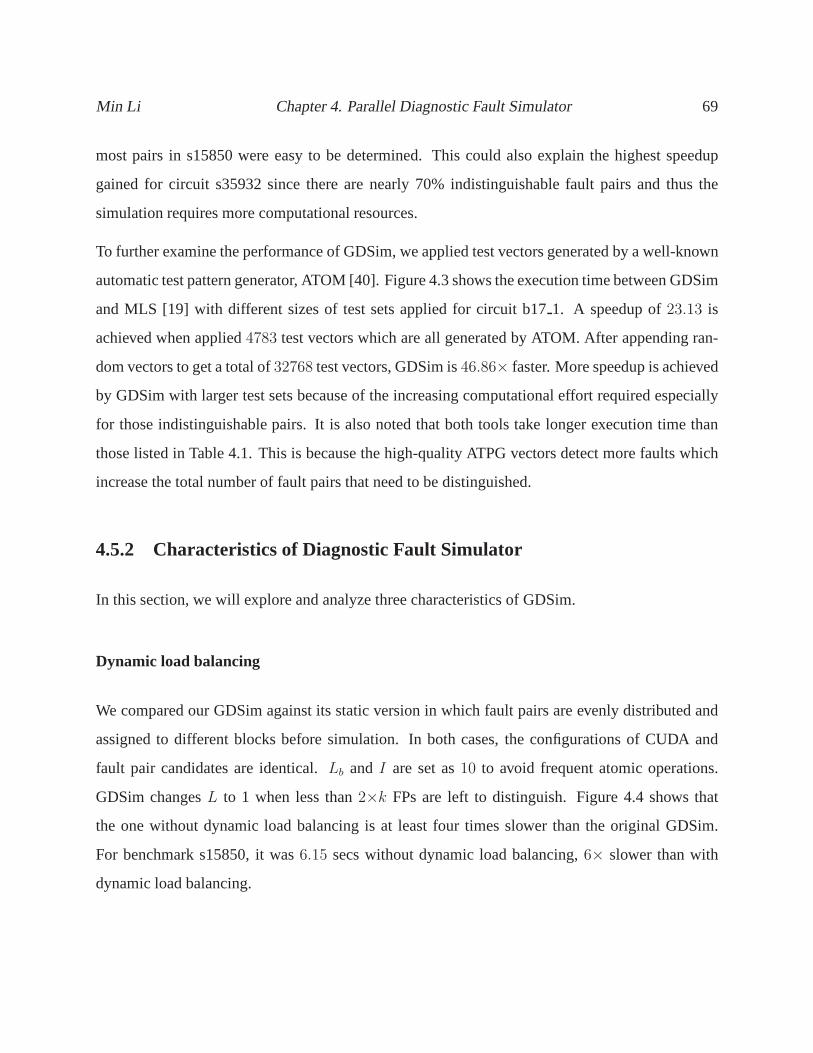
Min Li Chapter 4. Parallel Diagnostic Fault Simulator 69
most pairs in s15850 were easy to be determined. This could also explain the highest speedup
gained for circuit s35932 since there are nearly 70% indistinguishable fault pairs and thus the
simulation requires more computational resources.
To further examine the performance of GDSim, we applied testvectors generated by a well-known
automatic test pattern generator, ATOM [40]. Figure 4.3 shows the execution time between GDSim
and MLS [19] with different sizes of test sets applied for circuit b171. A speedup of23.13 is
achieved when applied4783 test vectors which are all generated by ATOM. After appending ran-
dom vectors to get a total of32768 test vectors, GDSim is46.86× faster. More speedup is achieved
by GDSim with larger test sets because of the increasing computational effort required especially
for those indistinguishable pairs. It is also noted that both tools take longer execution time than
those listed in Table 4.1. This is because the high-quality ATPG vectors detect more faults which
increase the total number of fault pairs that need to be distinguished.
4.5.2 Characteristics of Diagnostic Fault Simulator
In this section, we will explore and analyze three characteristics of GDSim.
Dynamic load balancing
We compared our GDSim against its static version in which fault pairs are evenly distributed and
assigned to different blocks before simulation. In both cases, the configurations of CUDA and
fault pair candidates are identical.Lb and I are set as10 to avoid frequent atomic operations.
GDSim changesL to 1 when less than2×k FPs are left to distinguish. Figure 4.4 shows that
the one without dynamic load balancing is at least four timesslower than the original GDSim.
For benchmark s15850, it was6.15 secs without dynamic load balancing,6× slower than with
dynamic load balancing.
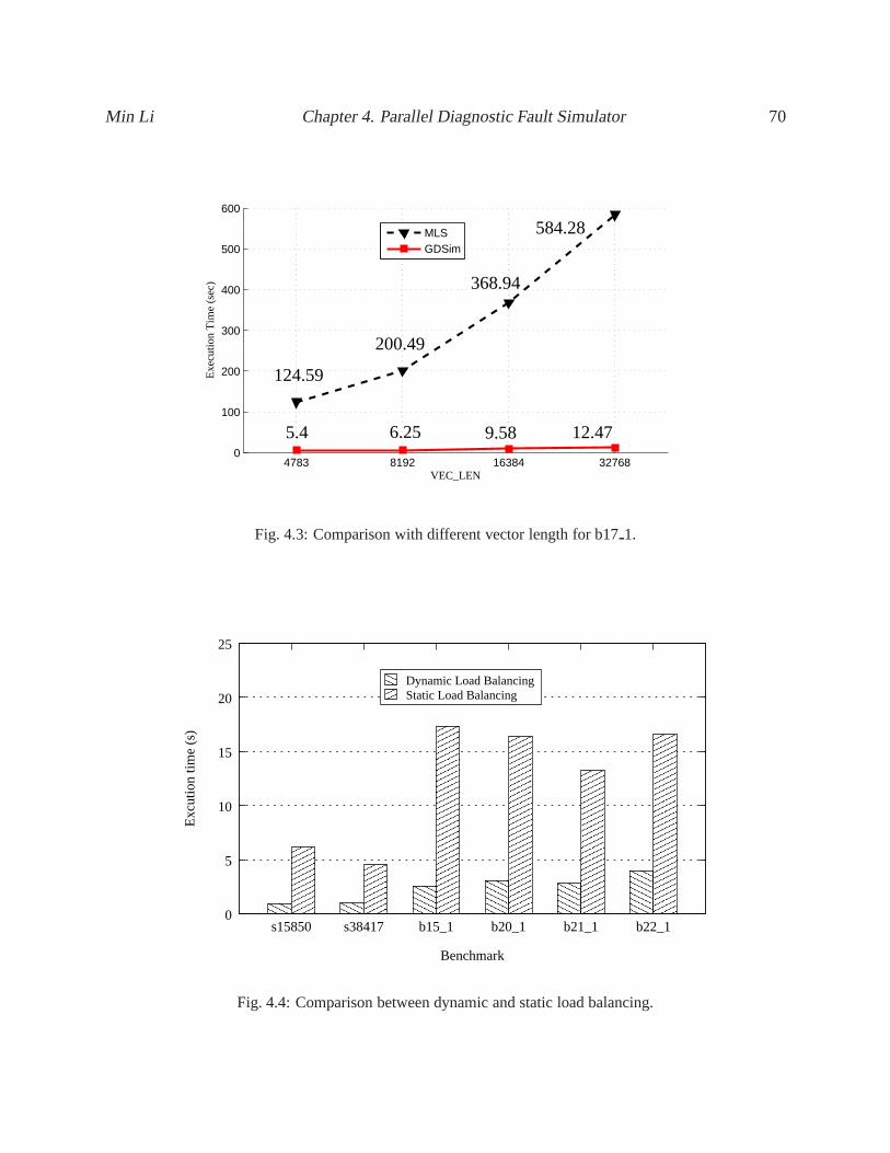
Min Li Chapter 4. Parallel Diagnostic Fault Simulator 70
4783 8192 16384 327680
100
200
300
400
500
600
VEC_LEN
Exe
cutio
n T
ime
(sec
)
MLSGDSim
5.4 6.25 9.58
200.49
368.94
12.47
584.28
124.59
Fig. 4.3: Comparison with different vector length for b171.
������������
��������
���������
���������
��������
��������
������������
������������
����������
����������
���������������������
���������������������
������������������
������������������
������������������������������������������������������
������������������������������������������������������
����������������������������������
����������������������������������
������������������������������������������
������������������������������������������
������������������������������������
������������������������������������
��������
����
0
5
10
15
20
25
s15850 s38417 b15_1 b20_1 b21_1 b22_1
Exc
utio
n tim
e (s
)
Benchmark
Dynamic Load BalancingStatic Load Balancing
Fig. 4.4: Comparison between dynamic and static load balancing.
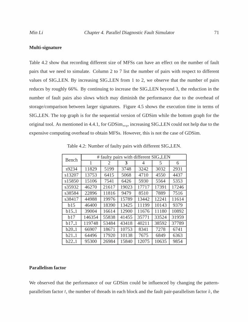
Min Li Chapter 4. Parallel Diagnostic Fault Simulator 71
Multi-signature
Table 4.2 show that recording different size of MFSs can havean effect on the number of fault
pairs that we need to simulate. Column 2 to 7 list the number ofpairs with respect to different
values of SIGLEN. By increasing SIGLEN from 1 to 2, we observe that the number of pairs
reduces by roughly 66%. By continuing to increase the SIGLEN beyond 3, the reduction in the
number of fault pairs also slows which may diminish the performance due to the overhead of
storage/comparison between larger signatures. Figure 4.5shows the execution time in terms of
SIG LEN. The top graph is for the sequential version of GDSim while the bottom graph for the
original tool. As mentioned in 4.4.1, for GDSimseq, increasing SIGLEN could not help due to the
expensive computing overhead to obtain MFSs. However, thisis not the case of GDSim.
Table 4.2: Number of faulty pairs with different SIGLEN.
Bench# faulty pairs with different SIGLEN
1 2 3 4 5 6s9234 11829 5199 3748 3242 3032 2931s13207 13753 6415 5068 4710 4550 4437s15850 15106 7541 6426 5930 5564 5353s35932 46270 21617 19023 17717 17391 17246s38584 22896 11816 9479 8510 7889 7516s38417 44988 19976 15789 13442 12241 11614
b15 46400 18390 13425 11199 10143 9379b15 1 39004 16614 12900 11676 11180 10892b17 146354 55838 41455 35771 33524 31959
b17 1 119748 53484 43418 40211 38592 37789b20 1 66907 18671 10753 8341 7278 6741b21 1 64496 17920 10138 7675 6849 6363b22 1 95300 26984 15840 12075 10635 9854
Parallelism factor
We observed that the performance of our GDSim could be influenced by changing the pattern-
parallelism factort, the number of threads in each block and the fault pair-parallelism factork, the
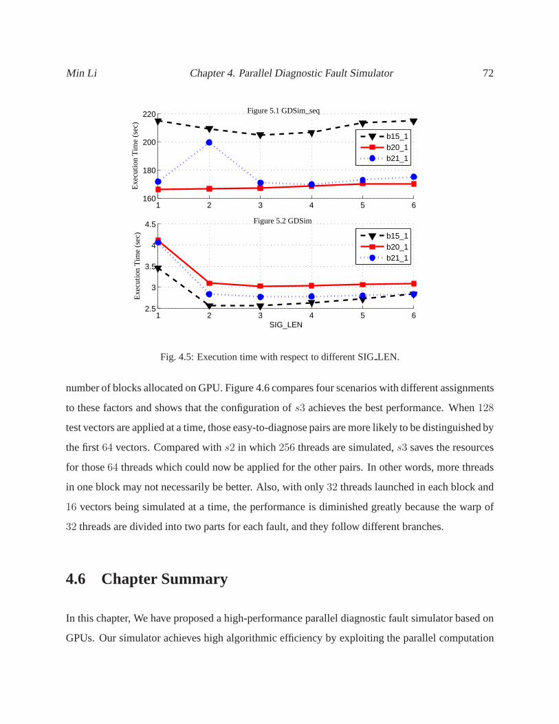
Min Li Chapter 4. Parallel Diagnostic Fault Simulator 72
1 2 3 4 5 6160
180
200
220
Exe
cutio
n T
ime
(sec
)
Figure 5.1 GDSim_seq
b15_1b20_1b21_1
1 2 3 4 5 62.5
3
3.5
4
4.5 Figure 5.2 GDSim
Exe
cutio
n T
ime
(sec
)
SIG_LEN
b15_1b20_1b21_1
Fig. 4.5: Execution time with respect to different SIGLEN.
number of blocks allocated on GPU. Figure 4.6 compares four scenarios with different assignments
to these factors and shows that the configuration ofs3 achieves the best performance. When128
test vectors are applied at a time, those easy-to-diagnose pairs are more likely to be distinguished by
the first64 vectors. Compared withs2 in which 256 threads are simulated,s3 saves the resources
for those64 threads which could now be applied for the other pairs. In other words, more threads
in one block may not necessarily be better. Also, with only32 threads launched in each block and
16 vectors being simulated at a time, the performance is diminished greatly because the warp of
32 threads are divided into two parts for each fault, and they follow different branches.
4.6 Chapter Summary
In this chapter, We have proposed a high-performance parallel diagnostic fault simulator based on
GPUs. Our simulator achieves high algorithmic efficiency byexploiting the parallel computation
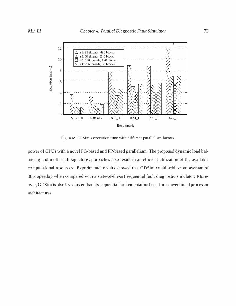
Min Li Chapter 4. Parallel Diagnostic Fault Simulator 73
�������
�������
��������
��������
����������������
����������������
����������������������������������
����������������������������������
����������������������������������
����������������������������������
�����������������������
�����������������������
���
���
����������
����������
������������������
������������������
�����������
�����������
�����������
�����������
��������������������������
��������������������������
����
����
���
���
��������������
��������������
���������
���������
����������������
����������������
������������������������
������������������������
������
������
������
������
����������
����������
������
������
�������
�������
��������
��������
��������
����
����
��������
0
2
4
6
8
10
12
S15,850 S38,417 b15_1 b20_1 b21_1 b22_1
Exc
utio
n tim
e (s
)
Benchmark
s1: 32 threads, 480 blockss2: 64 threads, 240 blockss3: 128 threads, 120 blockss4: 256 threads, 60 blocks
Fig. 4.6: GDSim’s execution time with different parallelism factors.
power of GPUs with a novel FG-based and FP-based parallelism. The proposed dynamic load bal-
ancing and multi-fault-signature approaches also result in an efficient utilization of the available
computational resources. Experimental results showed that GDSim could achieve an average of
38× speedup when compared with a state-of-the-art sequential fault diagnostic simulator. More-
over, GDSim is also 95× faster than its sequential implementation based on conventional processor
architectures.
Chapter 5
Parallel Reliablity Analysis
5.1 Chapter Overview
In this chapter, we present a parallel reliability analysistool of logic circuits on GPUs. In nano-
scale technologies, the reliability of logic circuits is emerging as an important concern due to
the reduced margins to both intrinsic and extrinsic noise. The computational complexity of reli-
ability analysis increases exponentially with the size of acircuit, making the previous analytical
approaches intractable for large circuits. RAG, an efficient parallel Reliability Analysis tool based
is a fault injection based parallel stochastic simulator implemented on a state-of-the-art GPU. A
two-stage simulation framework is proposed to exploit the high computation efficiency of GPUs.
RAG also achieves high memory and instruction bandwidth by optimizing the parallel execution on
GPUs. With a novel memory management, RAG could accurately analyze the reliability of large
circuits without sacrificing computational occupancy on GPUs. Experimental results demonstrate
the accuracy and performance of RAG. A speedup of up to 793× and 477× (with average speedup
of 353.24× and 116.04×) is achieved compared to two state-of-the-art CPU-based approaches for
reliability analysis.
The remainder of this chapter is organized as follows. A brief introduction is given in Section 5.2.
74
Min Li Chapter 5. Parallel Reliablity Analysis 75
Section 5.3 presents a background in reliability analysis including metrics and related works. Sec-
tion 5.4 outlines a high-level process view of the proposed method, with a detail description of
some critical approaches. The experimental results are reported in Section 5.5. Finally Section 5.6
summarizes the chapter.
5.2 Introduction
Reliability analysis, a process of evaluating the effects of errors due to both intrinsic noise and
external transients at individual transistors, gates, or logic blocks on the outputs of the logic circuit,
will play an important role for both today’s and tomorrow’s nano-scale circuits. The probability
of error due to manufacturing defects, process variation, aging and transient faults is believed
to sharply increase due to rapidly diminishing feature sizes and complex fabrication processes
[45, 63, 100, 13, 14]. Moreover, the non-deterministic characteristics of novel devices such as
carbon nanotubes, silicon nanowires and molecular electronics make the circuit more vulnerable
to these effects. This necessitates an efficient reliability analysis tool which is accurate, robust and
scalable with design size and complexity.
Due to the exponential number of input combinations and the difficulty to model gate failures,
the reliability analysis of logic circuits is computationally complex. Exact analysis methods, using
probabilistic transfer matrices (PTMs) [48, 49] and probabilistic decision diagrams (PDDs) [1], can
provide accurate reliability evaluation. Several analysis heuristics, on the other hand, have been
proposed to generate a highly accurate reliability estimation, such as probabilistic gate models
(PGMs) [24, 94, 41], Bayesian networks [86] and Markov random fields [8]. However, they all
suffer from the problem of exponential complexity and are therefore practically infeasible for even
mid-size circuits (with more than ten thousand gates). A simulation scheme based on stochastic
computational models (SCMs) is proposed in [22]. Although the approach advances in the linear
computational complexity and high accuracy, it requires significant runtimes for large benchmark
circuits to get an accurate estimation.
Min Li Chapter 5. Parallel Reliablity Analysis 76
In this chapter, we present RAG, an efficient Reliability Analysis tool on GPUs. RAG is a fault-
injection based parallel stochastic simulator for logic circuits. The main motivation is to harness
the computational power of GPUs to obtain a highly accurate reliability evaluation of logic circuits
within short runtimes. Experimental results show that RAG achieves one to two orders of magni-
tude speedup in comparison with the CPU-based analysis tools. We summarize our contributions
as follows.
• To the best of our knowledge, this is the first work that accelerates the reliability analysis of
logic circuits on a GPU platform.
• We introduce a two-stage hierarchical simulation framework to efficiently utilize the com-
putation power of the GPU without exceeding its memory limitation. All the fanout stems
in the circuit will be scheduled and processed in order. Within the fanout free region (FFR)
of each stem, all the logic gates are also arranged and simulated in sequence. Highly paral-
lel execution is achieved by launching thousands of active threads which evaluate the same
logic gate but with different vectors.
• We formulated the device memory assignment for fanout stemsas a scheduling problem and
propose a greedy heuristic to reduce the memory requirementfor GPU based simulation.
Therefore, more threads could be launched on the GPU to achieve full occupancy. Also, the
overhead of data communication between the host (CPU) and the device (GPU) is minimized
by re-using the individual device’s memory.
• RAG maximizes the memory bandwidth by using the low-latencyshared memory for storing
the values of gates within the FFR of each stem. A post-order tree traversal algorithm is
employed to tackle the problem of limited share memory resources.
• A novel data structure for storing circuit netlist is developed to exploit the memory hierarchy
of GPUs.
• We applied GPU-oriented performance optimization strategies to ensure a maximal speedup.
Global memory accesses are coalesced to achieve optimal memory bandwidth. A high in-
Min Li Chapter 5. Parallel Reliablity Analysis 77
struction bandwidth is obtained by avoiding branch divergence. RAG also takes advantage
of the inherent bit-parallelism of logic operations on computer words. The execution con-
figuration of each kernel launch is determined for efficiently mapping the algorithm on the
GPU.
5.3 Background
Based on fault injection and stochastic simulations illustrated in 2.2.3, RAG is capable of provid-
ing all the above metrics fromN random simulated samples. Suppose, a number ofN random
generated vectors are simulated and the fault free and faulty logic values for them outputs are
recorded asOi(j) andOei (j), respectively, wherei is the index of the outputs andj is the index
of the vectors. Since a single sample is simulated by one random input vector, this work use the
termssampleandvectorinterchangeably.
Then, the probability of error for each outputi, can be calculated as:
δi =ǫiN
=
∑N
j=1Oi(j)⊕Oei (j)
N, (5.1)
whereǫi is the number of faulty samples on outputi.
Similarly, the average reliability among all outputs (Ravg) is represent as:
Ravg =
∑m
i=1 (1− δi)
m. (5.2)
5.3.1 Previous Work
The authors in [48] employ probability transfer matrices (PTMs) to capture non-deterministic be-
havior in logic circuits. Since the occurrence probabilityof everyinput-output vector pair for each
level in the circuit has to be recorded, PTMs are not applicable for large benchmarks due to the
massive matrix storage and manipulation overhead. Although PTMs are extended to a reliability
Min Li Chapter 5. Parallel Reliablity Analysis 78
estimation using input vector sampling in [49], our resultsshow that RAG is more efficient and
can handle even bigger circuits with the same accuracy.
Three more scalable algorithms are proposed in [24] for reliability analysis, but for large circuits,
accuracy is achieved by constraining on error conditions which is the number of simultaneous
gate failures in the circuits (e.g., maximum-k gate failure can co-occur at any given time). In
the experiment results, the largest simultaneous gate failures is set to3. Also, to get an accurate
estimation of reliability, high correlation coefficients in signal probability computation have to be
used to handle the reconvergent fan-out. However, the algorithms do not scale well for mid-size
benchmarks.
In [22], a traditional approach to reliability analysis is proposed that employs fault injection and
simulation in a Monte Carlo framework. Although the algorithm is scalable,only 1000 samples
are simulated with a relatively high execution overhead. Our experimental results show that a large
sample size is required for logic circuits to obtain an accurate reliability analysis. The simulation
overhead is caused by adding exclusive-or gates for every logic device which makes the circuits
size two-times larger. Also, the random bit sequence generation during Monte Carlo simulation
requires a significant amount of runtime.
In RAG, we parallelized the Monte Carlo based simulation andimplemented it on GPUs. No
exclusive-or gates are needed to add into the circuits. A two-stage hierarchical simulation frame-
work is proposed to efficiently utilize the computation power of GPUs. Memory usage is optimized
to achieve full computational occupancy and high memory bandwidth on GPUs. Also, the process
of random number generation (RNG) is parallelized to minimize the overhead. By simulating mil-
lions of samples on thousands of threads running simultaneously on the GPU, RAG could achieve
a high accuracy of reliability evaluation for industry sizebenchmarks within a short runtime.
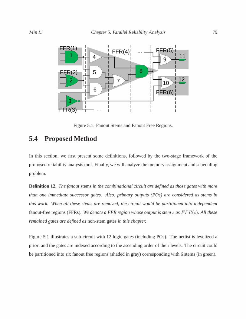
Min Li Chapter 5. Parallel Reliablity Analysis 79
1
2
5
6
7
9 11
12
FFR(1)
FFR(2)
FFR(4)
8
FFR(3)
10
...
...
3
4
FFR(6)
FFR(5)
Figure 5.1: Fanout Stems and Fanout Free Regions.
5.4 Proposed Method
In this section, we first present some definitions, followed by the two-stage framework of the
proposed reliability analysis tool. Finally, we will analyze the memory assignment and scheduling
problem.
Definition 12. The fanoutstemsin the combinational circuit are defined as those gates with more
than one immediate successor gates. Also, primary outputs (POs) are considered as stems in
this work. When all these stems are removed, the circuit would be partitioned into independent
fanout-free regions (FFRs). We denote a FFR region whose output is stems asFFR(s). All these
remained gates are defined asnon-stem gatesin this chapter.
Figure 5.1 illustrates a sub-circuit with 12 logic gates (including POs). The netlist is levelized a
priori and the gates are indexed according to the ascending order of their levels. The circuit could
be partitioned into six fanout free regions (shaded in gray)corresponding with 6 stems (in green).
Min Li Chapter 5. Parallel Reliablity Analysis 80
5.4.1 Framework
The high-level flow of RAG is shown in Figure 5.2, where the white boxes denote the CPU work-
load, and the shaded boxes are the GPU workload. At the beginning, the CPU reads in the circuit
netlist and generates the list of stems with the corresponding fanout free regions. A post-order tree
traversal algorithm is employed to the arrange the simulation sequence of gates (non-stem gates)
within each of the FFRs. Because we only need to store the stems’ values, the memory for the
FFRs can be shared, thus saving much space. After that, we formulate another scheduling for the
simulation of stem as an optimization problem whose objective is to minimize the memory storage
of logic values needed. In other words, we need not allocate memory to store the values for all
stems. Rather, storage of a stem’s value can be reused whenever all its successors (child stems)
have been evaluated. A greedy approach is employed in this scheduling algorithm to help RAG
further reduce the memory usage so as to achieve a high bandwidth and full occupancy during sim-
ulation. Then, the scheduled circuit netlist represented as a bit stream is transferred to the GPU. A
GPU-based stochastic simulatorksim is launched as Kernel 1 on the GPU. Thousands of threads
could be launched with each simulating a totalp random vectors. To avoid branch divergence,
each thread within the same warp evaluates the same logic gate simultaneously but with different
vectors. At the end of simulating each vector, the number of errors arrived at each output will
be recorded in vector~ǫ on global memory. Since each thread maintains its own error vectors, a
parallel reduction kernelkred is launched to compute the total number of errors for each outputs
and transfer the summed up~ǫ back to the CPU. The parallel reduction kernel is a modified version
of the one provided in CUDA software development kit (SDK) [72]. Finally, RAG will compute
the average error probability for each output,δ and theRavg to give a comprehensive reliability
analysis of the logic circuits.
Circuit Netlist with a bit stream
The netlist of the circuit is an array of logic gates. Their sequences are decided according to a
two-stage pre-processed scheduling. The stems are sorted according to a greedy algorithm and the
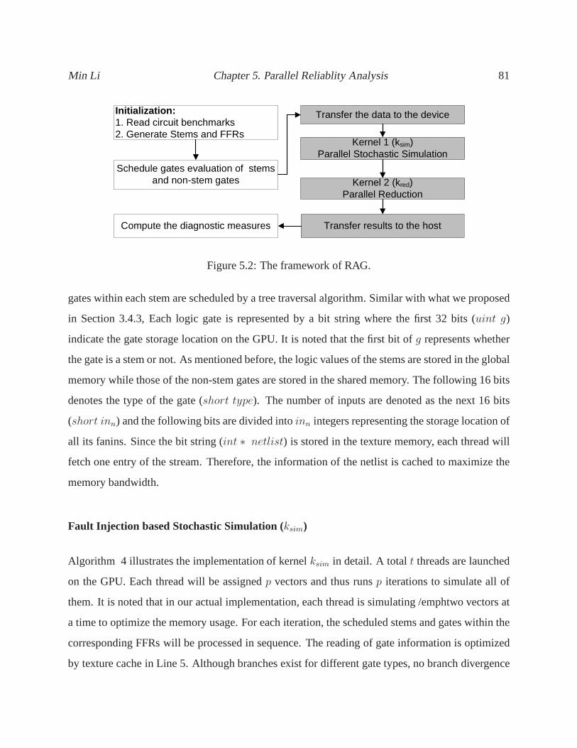
Min Li Chapter 5. Parallel Reliablity Analysis 81
Initialization:1. Read circuit benchmarks2. Generate Stems and FFRs
Transfer the data to the device
Kernel 1 (ksim)Parallel Stochastic Simulation
Transfer results to the hostCompute the diagnostic measures
Schedule gates evaluation of stems and non-stem gates Kernel 2 (kred)
Parallel Reduction
Figure 5.2: The framework of RAG.
gates within each stem are scheduled by a tree traversal algorithm. Similar with what we proposed
in Section 3.4.3, Each logic gate is represented by a bit string where the first 32 bits (uint g)
indicate the gate storage location on the GPU. It is noted that the first bit ofg represents whether
the gate is a stem or not. As mentioned before, the logic values of the stems are stored in the global
memory while those of the non-stem gates are stored in the shared memory. The following 16 bits
denotes the type of the gate (short type). The number of inputs are denoted as the next 16 bits
(short inn) and the following bits are divided intoinn integers representing the storage location of
all its fanins. Since the bit string (int ∗ netlist) is stored in the texture memory, each thread will
fetch one entry of the stream. Therefore, the information ofthe netlist is cached to maximize the
memory bandwidth.
Fault Injection based Stochastic Simulation (ksim)
Algorithm 4 illustrates the implementation of kernelksim in detail. A totalt threads are launched
on the GPU. Each thread will be assignedp vectors and thus runsp iterations to simulate all of
them. It is noted that in our actual implementation, each thread is simulating /emphtwo vectors at
a time to optimize the memory usage. For each iteration, the scheduled stems and gates within the
corresponding FFRs will be processed in sequence. The reading of gate information is optimized
by texture cache in Line 5. Although branches exist for different gate types, no branch divergence
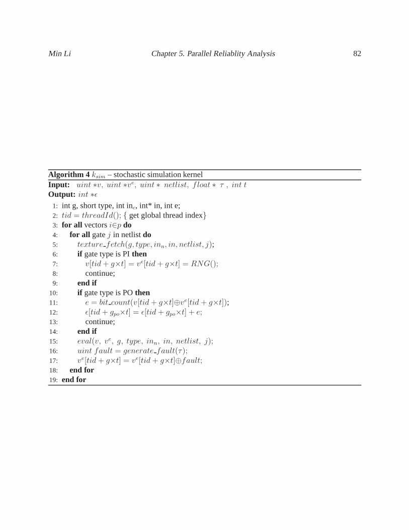
Min Li Chapter 5. Parallel Reliablity Analysis 82
Algorithm 4 ksim – stochastic simulation kernelInput: uint ∗v, uint ∗ve, uint ∗ netlist, f loat ∗ τ , int tOutput: int ∗ǫ
1: int g, short type, int inc, int* in, int e;2: tid = threadId(); { get global thread index}3: for all vectorsi∈p do4: for all gatej in netlistdo5: texture fetch(g, type, inn, in, netlist, j);6: if gate type is PIthen7: v[tid+ g×t] = ve[tid + g×t] = RNG();8: continue;9: end if
10: if gate type is POthen11: e = bit count(v[tid+ g×t]⊕ve[tid + g×t]);12: ǫ[tid + gpo×t] = ǫ[tid + gpo×t] + e;13: continue;14: end if15: eval(v, ve, g, type, inn, in, netlist, j);16: uint fault = generate fault(τ);17: ve[tid + g×t] = ve[tid + g×t]⊕fault;18: end for19: end for
Min Li Chapter 5. Parallel Reliablity Analysis 83
is introduced because all the threads within one warp are simulating the same gate simultaneously.
Therefore, it is guaranteed that all the threads within the same warp will be running on the same
branches but simulating different vectors. In line 15, we call the functioneval to evaluate both the
faulty and fault-free model of the circuit and recorded the value at locationg in vectors~v and ~ve,
respectively. In Line 16, the faults are generated by the a parallel random number generator (the
same used in Line 7) according to the error rate vector (~τ ). The implemented GPU based RNG is
similar with the one proposed in [96]. Faults are injected inLine 17 by flipping the logic values.
Since32 vectors are simulated on every thread concurrently, errorson each output are counted in
Line 11 and added to the vector~ǫ in Line 12. At the end of simulation of each vector, the number
of errors on each output will be recorded in vector~ǫ on the global memory.
Memory Requirement versus Performance
A typical requirement for good performance on CUDA is that the application should use a large
number of threads. Also, the accuracy of the reliability analysis by stochastic simulation depends
on a large number of samples. By simulating millions of samples with thousands threads running
concurrently, RAG could achieve a high performance and accuracy. However, the number of
threads that could be allocated on GPUs are limited by not only the intrinsic constraints of the
CUDA architecture, but also the total memory limitation (Mt). According to our experiments, the
storage for logic values,~v and ~ve dominates the memory usage. If the total number of threads
launched on GPUs ist, the memory requirement would beMv = V×4×t (each threads simulate 2
vectors at a time), whereV is the size of the space to store~v and~ve. Therefore, in order to achieve
high performance and accuracy with the limited memory, we propose a method to reduceV .
5.4.2 Scheduling of Stems
Definition 13. For a circuit with n stems, represented as~s = {s1, s2, . . . , sn}, we define their
corresponding simulation slots as~a = {a1, a2, . . . , an}, and their storage location on~v and ~ve as
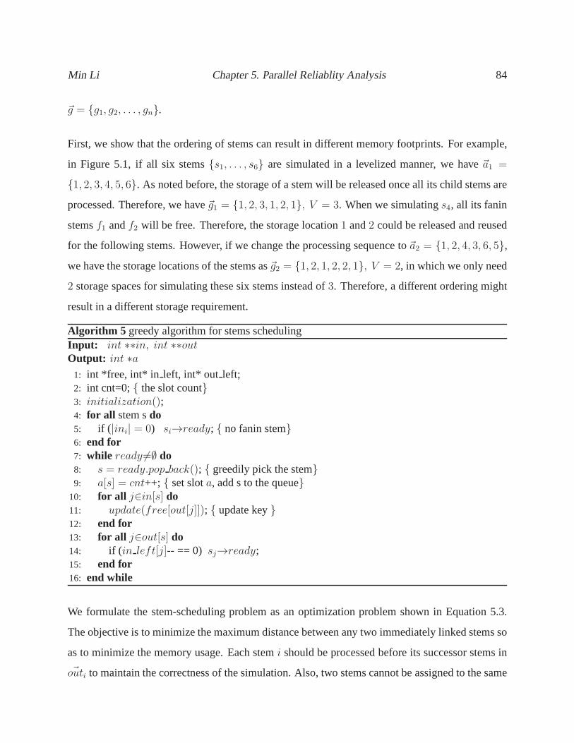
Min Li Chapter 5. Parallel Reliablity Analysis 84
~g = {g1, g2, . . . , gn}.
First, we show that the ordering of stems can result in different memory footprints. For example,
in Figure 5.1, if all six stems{s1, . . . , s6} are simulated in a levelized manner, we have~a1 =
{1, 2, 3, 4, 5, 6}. As noted before, the storage of a stem will be released once all its child stems are
processed. Therefore, we have~g1 = {1, 2, 3, 1, 2, 1}, V = 3. When we simulatings4, all its fanin
stemsf1 andf2 will be free. Therefore, the storage location1 and2 could be released and reused
for the following stems. However, if we change the processing sequence to~a2 = {1, 2, 4, 3, 6, 5},
we have the storage locations of the stems as~g2 = {1, 2, 1, 2, 2, 1}, V = 2, in which we only need
2 storage spaces for simulating these six stems instead of3. Therefore, a different ordering might
result in a different storage requirement.
Algorithm 5 greedy algorithm for stems schedulingInput: int ∗∗in, int ∗∗outOutput: int ∗a
1: int *free, int* in left, int* out left;2: int cnt=0;{ the slot count}3: initialization();4: for all stem sdo5: if ( |ini| = 0) si→ready; { no fanin stem}6: end for7: while ready 6=∅ do8: s = ready.pop back(); { greedily pick the stem}9: a[s] = cnt++; { set slota, add s to the queue}
10: for all j∈in[s] do11: update(free[out[j]]); { update key}12: end for13: for all j∈out[s] do14: if ( in left[j]-- == 0) sj→ready;15: end for16: end while
We formulate the stem-scheduling problem as an optimization problem shown in Equation 5.3.
The objective is to minimize the maximum distance between any two immediately linked stems so
as to minimize the memory usage. Each stemi should be processed before its successor stems in
~outi to maintain the correctness of the simulation. Also, two stems cannot be assigned to the same
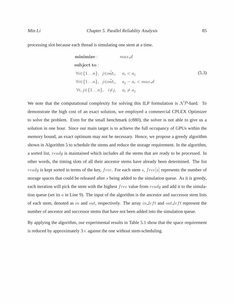
Min Li Chapter 5. Parallel Reliablity Analysis 85
processing slot because each thread is simulating one stem at a time.
minimize : max d
subject to :
∀i∈{1. . .n}, j∈ ~outi, ai < aj
∀i∈{1. . .n}, j∈ ~outi, aj − ai < max d
∀i, j∈{1. . .n}, i6=j, ai 6= aj
(5.3)
We note that the computational complexity for solving this ILP formulation isNP-hard. To
demonstrate the high cost of an exact solution, we employed acommercial CPLEX Optimizer
to solve the problem. Even for the small benchmark (c880), the solver is not able to give us a
solution in one hour. Since our main target is to achieve the full occupancy of GPUs within the
memory bound, an exact optimum may not be necessary. Hence, we propose a greedy algorithm
shown in Algorithm 5 to schedule the stems and reduce the storage requirement. In the algorithm,
a sorted list,ready is maintained which includes all the stems that are ready to be processed. In
other words, the timing slots of all their ancestor stems have already been determined. The list
ready is kept sorted in terms of the key,free. For each stems, free[s] represents the number of
storage spaces that could be released afters being added to the simulation queue. As it is greedy,
each iteration will pick the stem with the highestfree value fromready and add it to the simula-
tion queue (set itsa in Line 9). The input of the algorithm is the ancestor and successor stem lists
of each stem, denoted asin andout, respectively. The arrayin left andout left represent the
number of ancestor and successor stems that have not been added into the simulation queue.
By applying the algorithm, our experimental results in Table 5.1 show that the space requirement
is reduced by approximately 3× against the one without stem-scheduling.
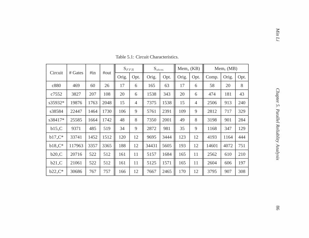
Min
LiC
hapter5.
ParallelR
eliablityA
nalysis8
6
Table 5.1: Circuit Characteristics.
Circuit # Gates #in #outSFFR Sstem Mems (KB) Memt (MB)
Orig. Opt. Orig. Opt. Orig. Opt. Comp. Orig. Opt.
c880 469 60 26 17 6 165 63 17 6 58 20 8
c7552 3827 207 108 20 6 1538 343 20 6 474 181 43
s35932* 19876 1763 2048 15 4 7375 1538 15 4 2506 913 240
s38584 22447 1464 1730 106 9 5761 2391 109 9 2812 717 329
s38417* 25585 1664 1742 48 8 7350 2001 49 8 3198 901 284
b15 C 9371 485 519 34 9 2872 981 35 9 1168 347 129
b17 C* 33741 1452 1512 120 12 9695 3444 123 12 4193 1164 444
b18 C* 117963 3357 3365 188 12 34431 5605 193 12 14601 4072 751
b20 C 20716 522 512 161 11 5157 1684 165 11 2562 610 210
b21 C 21061 522 512 161 11 5125 1571 165 11 2604 606 197
b22 C* 30686 767 757 166 12 7667 2465 170 12 3795 907 308
Min Li Chapter 5. Parallel Reliablity Analysis 87
5.4.3 Scheduling of Non-stem Gates
As suggested in 2.1, read/write on the shared memory has the advantage of low latency compared
with global memory. Therefore, storing the logic value of non-stem gates in the shared memory
would help reduce the read/write overhead. Since the gates in each FFR are simulated indepen-
dently, shared memory can be re-used for each FFR which makesit ideal for storing the values
of these gates. However, because only 16 KB share memory is available on each SM, we need to
reduce the maximum memory usage among the FFRs.
We also take FFR(4) in Figure 5.1 as an example with the same notation used in Section 5.4.2.
The original order~a1 = {4, 5, 6, 7, 8} results in the assignment,~g1 = {1, 2, 3, 2, 1}, V = 3.
However, if the gates are simulated by another order~a2 = {5, 6, 7, 4, 8}, the storage would be
~g2 = {1, 2, 1, 2, 1}, V = 2, which is one space less than the original one. Therefore, for each stem
s, we employ an approach based on the post-order tree traverseto determine the gate simulation
order within the FFR. Effectively, we consider the gates in FFR(s) as a tree. At the pre-processing
stage, for each node, its child nodes are sorted in terms of their number of child nodes. The node
with more child nodes are preferable to be simulated earlierso that more memory spaces could
be free. After that, another post-order tree traverse is processed to determine the gate simulation
order. By applying the algorithm, our experimental resultsshows that the space requirement for
simulating the FFRs can be reduced by more than 10× against the one without scheduling. More
importantly, the reduced memory requirement allows the storage of non-stem gates to fit into the
16KB shared memory without going through the global memory when simulating the gates in each
FFR.
5.5 Experimental Results
We evaluated RAG’s performance on a set of large ISCAS89 [15]and ITC99 [27] benchmark
circuits which are available from [44]. Our fault simulation platform consists of a workstation with
Intel Quad-core i7 3.33 GHz CPU, 2 GB memory and one NVIDIA GeForce GTX 285 graphics
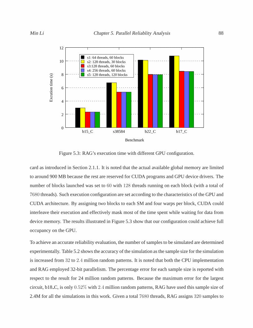
Min Li Chapter 5. Parallel Reliablity Analysis 88
0
2
4
6
8
10
12
b15_C s38584 b22_C b17_C
Exc
utio
n tim
e (s
)
Benchmark
s1: 64 threads, 60 blockss2: 128 threads, 30 blockss3:128 threads, 60 blockss4: 256 threads, 60 blockss5: 128 threads, 120 blocks
Figure 5.3: RAG’s execution time with different GPU configuration.
card as introduced in Section 2.1.1. It is noted that the actual available global memory are limited
to around 900 MB because the rest are reserved for CUDA programs and GPU device drivers. The
number of blocks launched was set to60 with 128 threads running on each block (with a total of
7680 threads). Such execution configuration are set according tothe characteristics of the GPU and
CUDA architecture. By assigning two blocks to each SM and four warps per block, CUDA could
interleave their execution and effectively mask most of thetime spent while waiting for data from
device memory. The results illustrated in Figure 5.3 show that our configuration could achieve full
occupancy on the GPU.
To achieve an accurate reliability evaluation, the number of samples to be simulated are determined
experimentally. Table 5.2 shows the accuracy of the simulation as the sample size for the simulation
is increased from32 to 2.4 million random patterns. It is noted that both the CPU implementation
and RAG employed 32-bit parallelism. The percentage error for each sample size is reported with
respect to the result for 24 million random patterns. Because the maximum error for the largest
circuit, b18C, is only0.52% with 2.4 million random patterns, RAG have used this sample size of
2.4M for all the simulations in this work. Given a total7680 threads, RAG assigns320 samples to
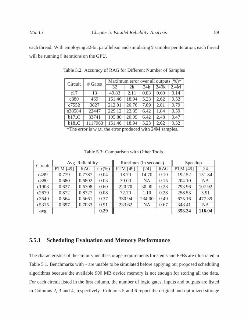
Min Li Chapter 5. Parallel Reliablity Analysis 89
each thread. With employing 32-bit parallelism and simulating2 samples per iteration, each thread
will be running5 iterations on the GPU.
Table 5.2: Accuracy of RAG for Different Number of Samples
Circuit # GatesMaximum error over all outputs (%)*
32 2k 24k 240k 2.4Mc17 13 49.83 2.11 0.83 0.69 0.14c880 469 151.46 18.94 5.23 2.62 0.52c7552 3827 212.01 20.76 7.89 2.81 0.79s38584 22447 229.12 22.35 6.42 1.84 0.59b17 C 33741 105.80 20.09 6.42 2.48 0.47b18 C 1117963 151.46 18.94 5.23 2.62 0.52*The error is w.r.t. the error produced with 24M samples.
Table 5.3: Comparison with Other Tools.
CircuitAvg. Reliability Runtimes (in seconds) Speedup
PTM [49] RAG err(%) PTM [49] [24] RAG PTM [49] [24]c499 0.779 0.7787 0.04 18.70 14.70 0.10 192.52 151.34c880 0.680 0.6802 0.03 30.00 NA 0.15 204.10 NAc1908 0.627 0.6308 0.60 220.70 30.00 0.28 793.96 107.92c2670 0.872 0.8727 0.08 72.70 1.10 0.28 258.53 3.91c3540 0.564 0.5661 0.37 330.94 234.00 0.49 675.16 477.39c5315 0.697 0.7033 0.91 233.62 NA 0.67 348.41 NAavg 0.29 353.24 116.04
5.5.1 Scheduling Evaluation and Memory Performance
The characteristics of the circuits and the storage requirements for stems and FFRs are illustrated in
Table 5.1. Benchmarks with∗ are unable to be simulated before applying our proposed scheduling
algorithms because the available 900 MB device memory is notenough for storing all the data.
For each circuit listed in the first column, the number of logic gates, inputs and outputs are listed
in Columns 2, 3 and 4, respectively. Columns 5 and 6 report theoriginal and optimized storage
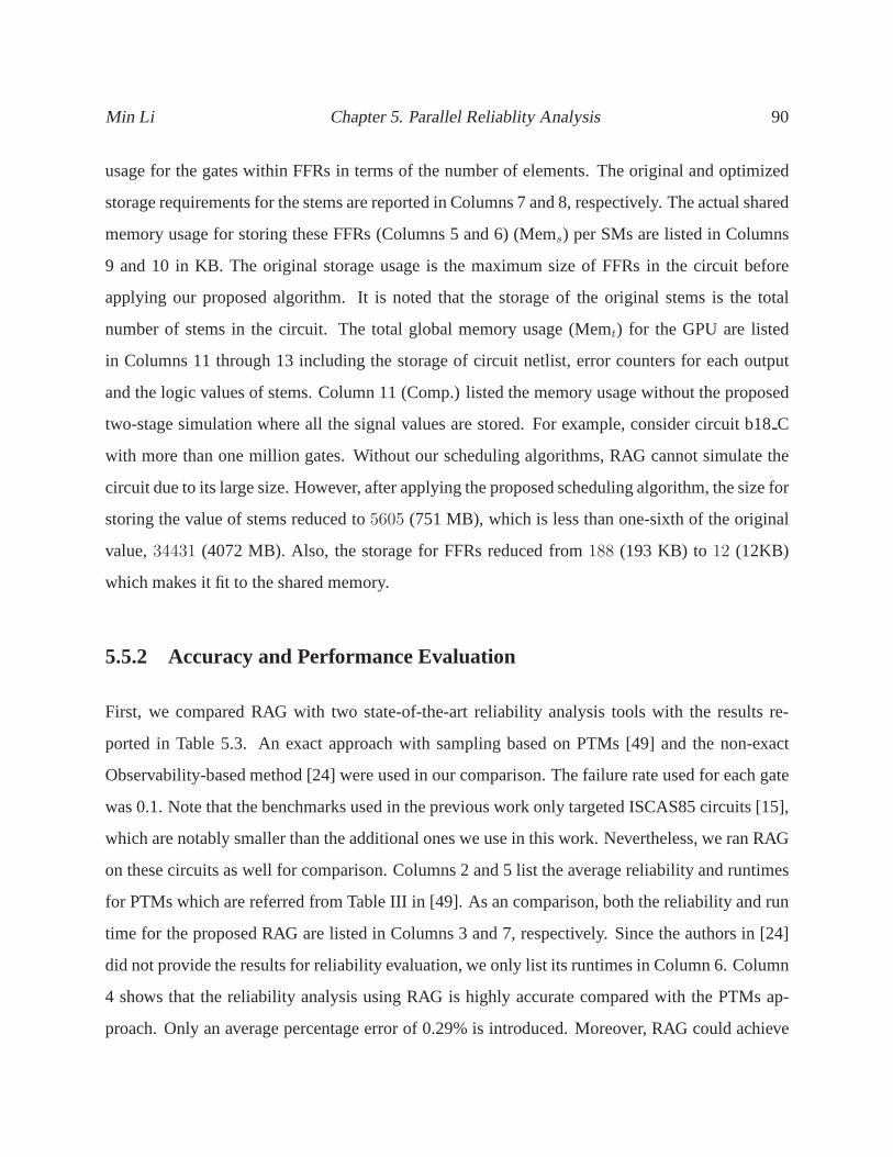
Min Li Chapter 5. Parallel Reliablity Analysis 90
usage for the gates within FFRs in terms of the number of elements. The original and optimized
storage requirements for the stems are reported in Columns 7and 8, respectively. The actual shared
memory usage for storing these FFRs (Columns 5 and 6) (Mems) per SMs are listed in Columns
9 and 10 in KB. The original storage usage is the maximum size of FFRs in the circuit before
applying our proposed algorithm. It is noted that the storage of the original stems is the total
number of stems in the circuit. The total global memory usage(Memt) for the GPU are listed
in Columns 11 through 13 including the storage of circuit netlist, error counters for each output
and the logic values of stems. Column 11 (Comp.) listed the memory usage without the proposed
two-stage simulation where all the signal values are stored. For example, consider circuit b18C
with more than one million gates. Without our scheduling algorithms, RAG cannot simulate the
circuit due to its large size. However, after applying the proposed scheduling algorithm, the size for
storing the value of stems reduced to5605 (751 MB), which is less than one-sixth of the original
value,34431 (4072 MB). Also, the storage for FFRs reduced from188 (193 KB) to 12 (12KB)
which makes it fit to the shared memory.
5.5.2 Accuracy and Performance Evaluation
First, we compared RAG with two state-of-the-art reliability analysis tools with the results re-
ported in Table 5.3. An exact approach with sampling based onPTMs [49] and the non-exact
Observability-based method [24] were used in our comparison. The failure rate used for each gate
was 0.1. Note that the benchmarks used in the previous work only targeted ISCAS85 circuits [15],
which are notably smaller than the additional ones we use in this work. Nevertheless, we ran RAG
on these circuits as well for comparison. Columns 2 and 5 listthe average reliability and runtimes
for PTMs which are referred from Table III in [49]. As an comparison, both the reliability and run
time for the proposed RAG are listed in Columns 3 and 7, respectively. Since the authors in [24]
did not provide the results for reliability evaluation, we only list its runtimes in Column 6. Column
4 shows that the reliability analysis using RAG is highly accurate compared with the PTMs ap-
proach. Only an average percentage error of 0.29% is introduced. Moreover, RAG could achieve
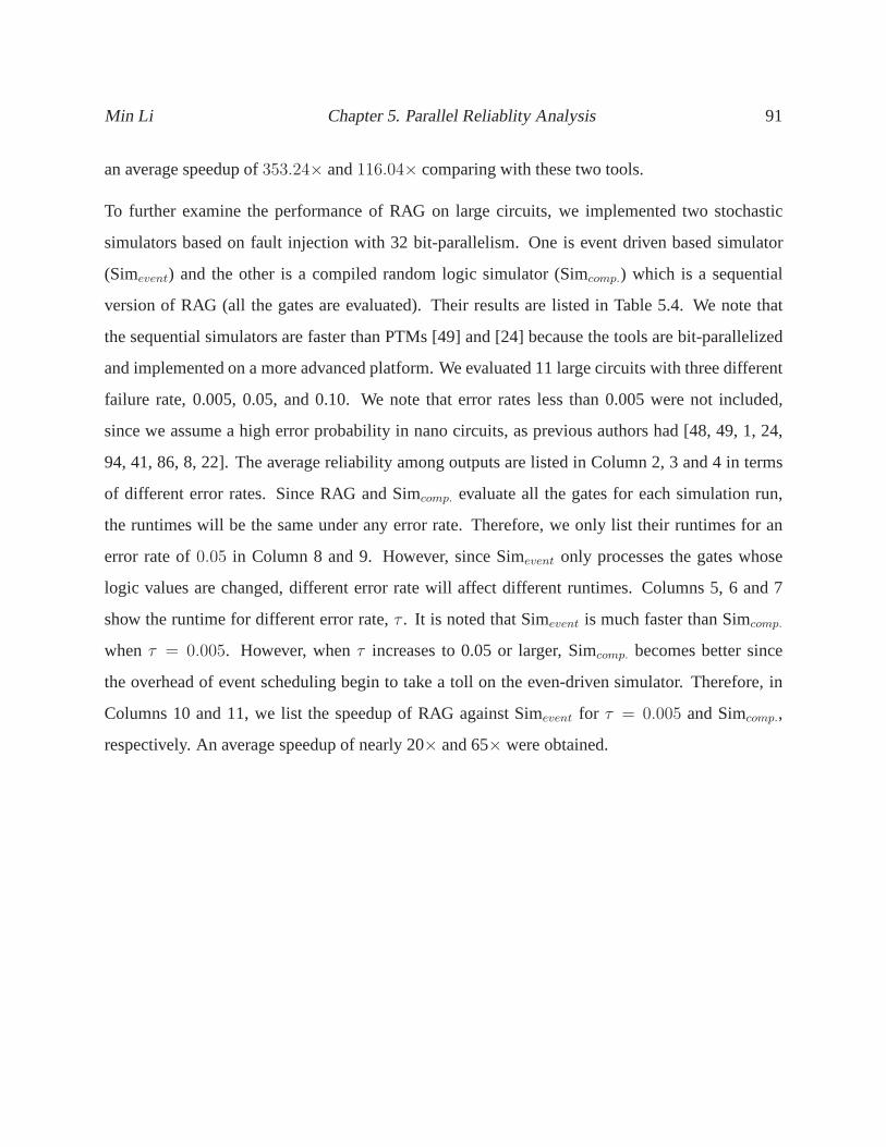
Min Li Chapter 5. Parallel Reliablity Analysis 91
an average speedup of353.24× and116.04× comparing with these two tools.
To further examine the performance of RAG on large circuits,we implemented two stochastic
simulators based on fault injection with 32 bit-parallelism. One is event driven based simulator
(Simevent) and the other is a compiled random logic simulator (Simcomp.) which is a sequential
version of RAG (all the gates are evaluated). Their results are listed in Table 5.4. We note that
the sequential simulators are faster than PTMs [49] and [24]because the tools are bit-parallelized
and implemented on a more advanced platform. We evaluated 11large circuits with three different
failure rate, 0.005, 0.05, and 0.10. We note that error ratesless than 0.005 were not included,
since we assume a high error probability in nano circuits, asprevious authors had [48, 49, 1, 24,
94, 41, 86, 8, 22]. The average reliability among outputs arelisted in Column 2, 3 and 4 in terms
of different error rates. Since RAG and Simcomp. evaluate all the gates for each simulation run,
the runtimes will be the same under any error rate. Therefore, we only list their runtimes for an
error rate of0.05 in Column 8 and 9. However, since Simevent only processes the gates whose
logic values are changed, different error rate will affect different runtimes. Columns 5, 6 and 7
show the runtime for different error rate,τ . It is noted that Simevent is much faster than Simcomp.
when τ = 0.005. However, whenτ increases to 0.05 or larger, Simcomp. becomes better since
the overhead of event scheduling begin to take a toll on the even-driven simulator. Therefore, in
Columns 10 and 11, we list the speedup of RAG against Simevent for τ = 0.005 and Simcomp.,
respectively. An average speedup of nearly 20× and 65× were obtained.
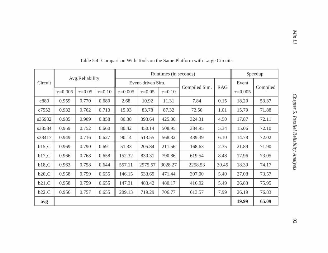
Min
LiC
hapter5.
ParallelR
eliablityA
nalysis9
2
Table 5.4: Comparison With Tools on the Same Platform with Large Circuits
CircuitAvg.Reliability
Runtimes (in seconds) Speedup
Event-driven Sim.Compiled Sim. RAG
EventCompiled
τ=0.005 τ=0.05 τ=0.10 τ=0.005 τ=0.05 τ=0.10 τ=0.005
c880 0.959 0.770 0.680 2.68 10.92 11.31 7.84 0.15 18.20 53.37
c7552 0.932 0.762 0.713 15.93 83.78 87.32 72.50 1.01 15.79 71.88
s35932 0.985 0.909 0.858 80.38 393.64 425.30 324.31 4.50 17.87 72.11
s38584 0.959 0.752 0.660 80.42 450.14 508.95 384.95 5.34 15.06 72.10
s38417 0.949 0.716 0.627 90.14 513.55 568.32 439.39 6.10 14.78 72.02
b15 C 0.969 0.790 0.691 51.33 205.84 211.56 168.63 2.35 21.89 71.90
b17 C 0.966 0.768 0.658 152.32 830.31 790.86 619.54 8.48 17.96 73.05
b18 C 0.963 0.758 0.644 557.11 2975.57 3028.27 2258.53 30.45 18.30 74.17
b20 C 0.958 0.759 0.655 146.15 533.69 471.44 397.00 5.40 27.08 73.57
b21 C 0.958 0.759 0.655 147.31 483.42 480.17 416.92 5.49 26.83 75.95
b22 C 0.956 0.757 0.655 209.13 719.29 706.77 613.57 7.99 26.19 76.83
avg 19.99 65.09
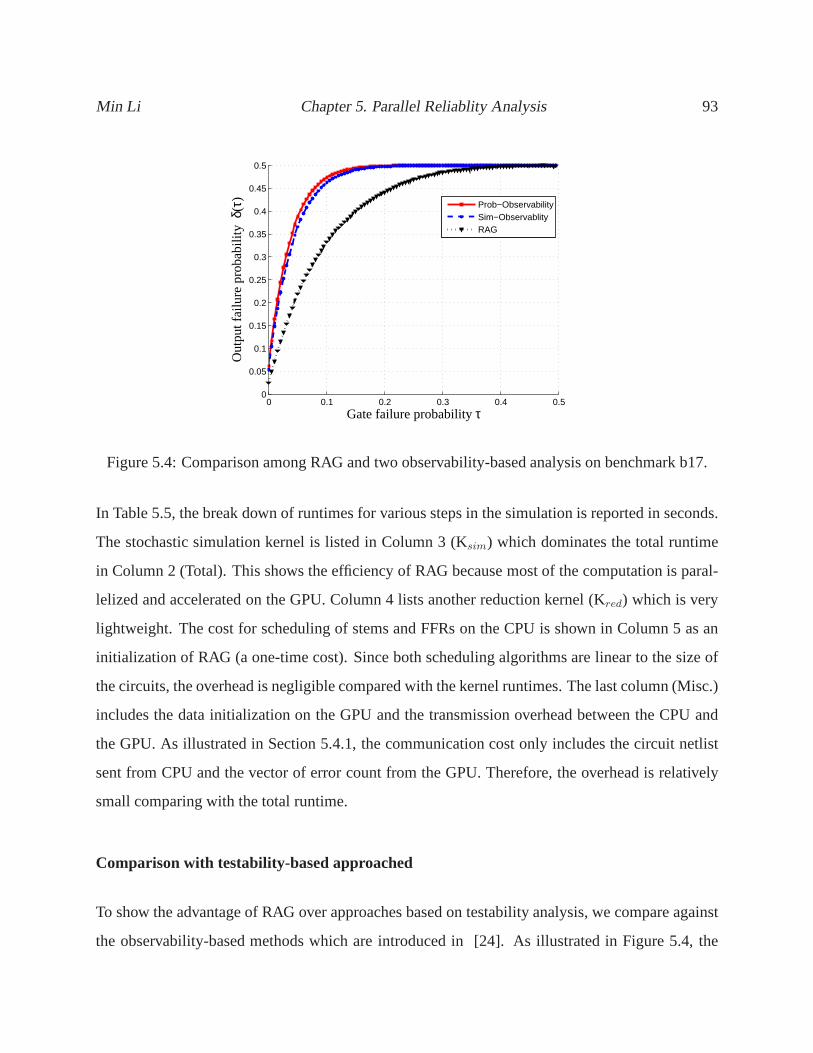
Min Li Chapter 5. Parallel Reliablity Analysis 93
0 0.1 0.2 0.3 0.4 0.50
0.05
0.1
0.15
0.2
0.25
0.3
0.35
0.4
0.45
0.5
Gate failure probability τ
Out
put f
ailu
re p
roba
bilit
y δ(τ)
Prob−ObservabilitySim−ObservablityRAG
Figure 5.4: Comparison among RAG and two observability-based analysis on benchmark b17.
In Table 5.5, the break down of runtimes for various steps in the simulation is reported in seconds.
The stochastic simulation kernel is listed in Column 3 (Ksim) which dominates the total runtime
in Column 2 (Total). This shows the efficiency of RAG because most of the computation is paral-
lelized and accelerated on the GPU. Column 4 lists another reduction kernel (Kred) which is very
lightweight. The cost for scheduling of stems and FFRs on theCPU is shown in Column 5 as an
initialization of RAG (a one-time cost). Since both scheduling algorithms are linear to the size of
the circuits, the overhead is negligible compared with the kernel runtimes. The last column (Misc.)
includes the data initialization on the GPU and the transmission overhead between the CPU and
the GPU. As illustrated in Section 5.4.1, the communicationcost only includes the circuit netlist
sent from CPU and the vector of error count from the GPU. Therefore, the overhead is relatively
small comparing with the total runtime.
Comparison with testability-based approached
To show the advantage of RAG over approaches based on testability analysis, we compare against
the observability-based methods which are introduced in [24]. As illustrated in Figure 5.4, the
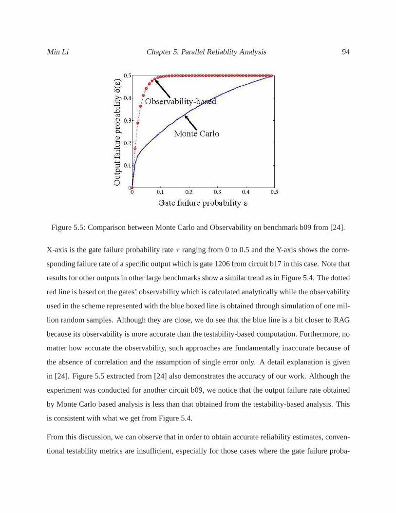
Min Li Chapter 5. Parallel Reliablity Analysis 94
Figure 5.5: Comparison between Monte Carlo and Observability on benchmark b09 from [24].
X-axis is the gate failure probability rateτ ranging from 0 to 0.5 and the Y-axis shows the corre-
sponding failure rate of a specific output which is gate 1206 from circuit b17 in this case. Note that
results for other outputs in other large benchmarks show a similar trend as in Figure 5.4. The dotted
red line is based on the gates’ observability which is calculated analytically while the observability
used in the scheme represented with the blue boxed line is obtained through simulation of one mil-
lion random samples. Although they are close, we do see that the blue line is a bit closer to RAG
because its observability is more accurate than the testability-based computation. Furthermore, no
matter how accurate the observability, such approaches arefundamentally inaccurate because of
the absence of correlation and the assumption of single error only. A detail explanation is given
in [24]. Figure 5.5 extracted from [24] also demonstrates the accuracy of our work. Although the
experiment was conducted for another circuit b09, we noticethat the output failure rate obtained
by Monte Carlo based analysis is less than that obtained fromthe testability-based analysis. This
is consistent with what we get from Figure 5.4.
From this discussion, we can observe that in order to obtain accurate reliability estimates, conven-
tional testability metrics are insufficient, especially for those cases where the gate failure proba-
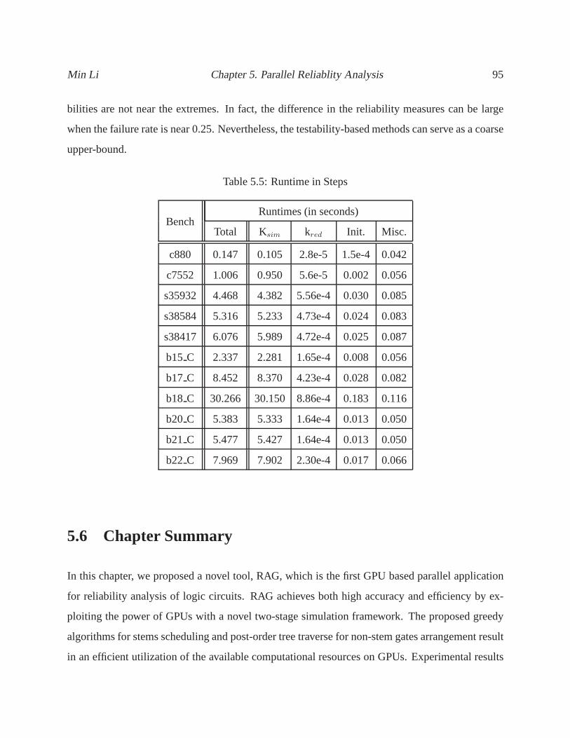
Min Li Chapter 5. Parallel Reliablity Analysis 95
bilities are not near the extremes. In fact, the difference in the reliability measures can be large
when the failure rate is near 0.25. Nevertheless, the testability-based methods can serve as a coarse
upper-bound.
Table 5.5: Runtime in Steps
BenchRuntimes (in seconds)
Total Ksim kred Init. Misc.
c880 0.147 0.105 2.8e-5 1.5e-4 0.042
c7552 1.006 0.950 5.6e-5 0.002 0.056
s35932 4.468 4.382 5.56e-4 0.030 0.085
s38584 5.316 5.233 4.73e-4 0.024 0.083
s38417 6.076 5.989 4.72e-4 0.025 0.087
b15 C 2.337 2.281 1.65e-4 0.008 0.056
b17 C 8.452 8.370 4.23e-4 0.028 0.082
b18 C 30.266 30.150 8.86e-4 0.183 0.116
b20 C 5.383 5.333 1.64e-4 0.013 0.050
b21 C 5.477 5.427 1.64e-4 0.013 0.050
b22 C 7.969 7.902 2.30e-4 0.017 0.066
5.6 Chapter Summary
In this chapter, we proposed a novel tool, RAG, which is the first GPU based parallel application
for reliability analysis of logic circuits. RAG achieves both high accuracy and efficiency by ex-
ploiting the power of GPUs with a novel two-stage simulationframework. The proposed greedy
algorithms for stems scheduling and post-order tree traverse for non-stem gates arrangement result
in an efficient utilization of the available computational resources on GPUs. Experimental results
Min Li Chapter 5. Parallel Reliablity Analysis 96
showed that RAG could achieve an average of 353× and 116× speedup against two state-of-the-art
reliability analysis tools (one is an exact approach with sampling and the other is heuristic-based)
without compromising accuracy. Moreover, for large benchmarks which are not able to be handled
efficiently by previous tools, RAG is also 20× ad 65× faster than another two stochastic simulation
based reliability analysis tools implemented on conventional processor architectures.
Chapter 6
Parallel Design Validation with a Modified
Ant Colony Optimization
6.1 Chapter Overview
In this chapter, we propose a novel parallel state justification tool, GACO, utilizing Ant Colony
Optimization (ACO) on Graphical Processing Units (GPU). With the high degree of parallelism
supported by the GPU, GACO is capable of launching a large number of artificial ants to search
for the target state. A novel parallel simulation technique, utilizing partitioned navigation tracks
as guides during the search, is proposed to achieve extremely high computation efficiency for
state justification. We present the results on a GPU platformfrom NVIDIA (a GeForce GTX 285
graphics card) that demonstrate a speedup of up to 228× compared to deterministic methods and
a speedup of up to 40× over previous state-of-the-art heuristic based serial tools.
The rest of this chapter is organized as follows. A brief introduction is given in Section 6.2.
In Section 6.3, we review the previous works in the area of state justification and introduce the
correlation based partition construction. Section 6.4 outlines a high-level process view of the
parallel logic simulator, built on the techniques utilizedin FSimGP2[54], with detail description of
97
Min Li Chapter 6. Parallel Design Validation with a Modified Ant Colony Optimization 98
the critical approaches. The experimental results are reported in Section 6.5. Finally, Section 6.6
gives the conclusion.
6.2 Introduction
State Justification is an important engine for test and verification. There may be important states
and transitions that need to be verified to ensure the correctfunctionality of the chip which neces-
sitate reaching of corner states. In addition, some design errors and bugs can only be exercised and
propagated by reaching specific states. Therefore, finding vectors that can reach these states from
known reachable states plays a critical role in design validation. Due to the exponential growth
in circuit size predicted by Moore’s Law, state justification has become increasingly difficult, as
modern circuits have hundreds of thousands to millions of flip-flops. This growth means that de-
terministically justifying the state will encounter scalability issues. For example, formal methods
such as model checking potentially requires traversing large portions of the state space to find a
solution. Dynamic, or simulation based approaches, on the other hand, can handle large circuits
but may not yield solutions for hard validation instances. Ahybrid formal and dynamic methods,
also known as semi-formal methods, offer promise. In semi-formal methods, formal techniques are
used on an abstraction of the design and simulation on the concrete design. However, simulation
is now also becoming a burden as circuits are becoming extremely large.
In order to help make design validation both efficient and scalable, we propose a semi-formal tech-
nique that utilizes Ant Colony Optimization (ACO) [31] based search on Graphic Processing Units
(GPUs). The abstraction is created by mining highly relatedstate variables from logic simulation
and partitioning them into groups. These groups are then analyzed deterministically to find their
distances from the target state. To further improve the performance and reduce simulation over-
head, graphic processing units are used to simulate the colony of artificial ants in parallel. Using
these distance metrics, we implemented a modified ant colonyoptimization algorithm on the GPUs
to guide the search towards the target state.
Min Li Chapter 6. Parallel Design Validation with a Modified Ant Colony Optimization 99
We have developed a novel ACO based State Justification Tool accelerated on GPUs, called GACO.
GACO harnesses the computational power of both swarm intelligence and modern day GPUs to
justify the state information for large circuits. Our method exploits pattern-parallelism with an ef-
ficient logic simulation tool that is capable of effectivelyutilizing memory bandwidth and massive
data parallelism on the GPU. The overhead of data communication between the host (CPU) and
the device (GPU) is minimized by utilizing as much of the individual device’s memory as possi-
ble. GACO also takes advantage of the inherent bit-parallelism of logic operations on computer
words. Additionally, due to the nature of GPUs, we are able tolaunch many more ants than previ-
ous methods and still achieve significant speedups. More ants allow us to explore a larger search
space, while parallel simulation on GPUs allows us to reduceexecution costs. The technique is
implemented on the NVIDIA GeForce GTX 285 with 30 cores and 8 SIMT execution pipelines
per core [59]. Our experimental results demonstrate that the proposed GACO can achieve between
one and two orders of magnitude speedup in comparison with the state-of-the-art sequential ACO
based state justification algorithm [53] implemented on conventional processor architecture.
6.3 Background
6.3.1 Previous Work
Formal verification provides the complete proof at the cost of both space and time in complex de-
signs. On the other hand, conventional simulation-based techniques are incapable of reaching some
hard-to-reach states. In order to mitigate the weaknesses of these two approaches, several hybrid
techniques have been proposed to combine and complement thestrengths of formal techniques and
simulation. Among these, the early pioneers in [99] proposed a direct random simulator under an
enlarged set of targets by computing preimages of the initial goal. Thus, the state is reachable if any
candidates in the enlarged set is hit. However, because of the design complexity, it is often infea-
sible to compute the complete set with the original circuit.To overcome the memory explosion for
computing the exact reachability of the target state(s), researchers proposed the abstraction-guided
Min Li Chapter 6. Parallel Design Validation with a Modified Ant Colony Optimization 100
simulation, in which formal methods are applied to an abstract model of the original circuit. An
abstract model is simply a reduced circuit model that retains a portion of the original (concrete)
circuit’s characteristics. A popular abstraction approach is to convert some flip-flops in the original
circuit to primary inputs, thereby reducing the state spaceof the abstract model. Note that by such
an abstraction, the state space results in an superset of theoriginal reachable space. That is, any
state reachable in the original design is also reachable in the abstract model, but not vice versa.
For example, suppose the original circuit has four flip-flops, and the abstract model has only the
first two of the four flip-flops. Then, among the original statespace of24 = 16 states, suppose the
state 1100 is the only unreachable state in the original concrete model, then in the abstract circuit,
since the latter 2 flip-flops are now fully controllable, 1100would be considered reachable in this
abstract model. Although inaccuracies are introduced, thesimplified abstract model makes formal
analysis feasible. And the resulting abstract state transition model, including the distances among
abstract states, is used to guide the search towards a targetstate of interest [90, 68, 34, 78].
The authors in [90] proposed a high-level abstraction modelthat closely interacts with the prop-
erty to be verified. The reachability of the target property is computed on this abstract circuit,
and the distance information is used to guide a simulator towards the target in a greedy manner.
However, due to the inaccuracy of the abstract model, the search can be stuck in a local optimal
point. Although a SAT engine is employed to bridge gaps between the current and the next closest
abstract state, the cost of using such tools may become expensive. To overcome the inaccuracy
of the approximate distance metric, an abstraction refinement strategy was introduce in [68]. Dur-
ing the process of state justification, some of the abstracted state variables are refined (restored
back) to the abstract circuit to make the abstract model moreclosely resemble the concrete circuit.
One drawback of this approach is that the cost of formal analysis increases exponentially for each
refinement of the circuit. Similar with the previous works, aBMC is applied in [78] to guide
the search process through narrow paths towards the target states for corner cases. Although the
authors employed a GA-based search engine, it is still hard to get out of the local optimal space
without using a BMC. Thus, such a method takes more time to reach the target states. Different
from the techniques that resort to full formal techniques asa back-up tactic to resolve the local
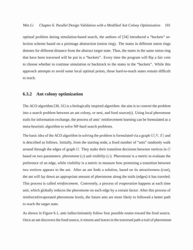
Min Li Chapter 6. Parallel Design Validation with a Modified Ant Colony Optimization 101
optimal problem during simulation-based search, the authors of [34] introduced a “buckets” se-
lection scheme based on a preimage abstraction (onion ring). The states in different onion rings
denotes for different distance from the abstract target state. Thus, the states in the same onion ring
that have been traversed will be put in a “buckets”. Every time the program will flip a fair coin
to choose whether to continue simulation or backtrack to thestates in the “buckets”. While this
approach attempts to avoid some local optimal points, thosehard-to-reach states remain difficult
to reach.
6.3.2 Ant colony optimization
The ACO algorithm [30, 31] is a biologically inspired algorithm: the aim is to convert the problem
into a search problem between an ant colony, or nest, and foodsource(s). Using local pheromone
trails for information exchange, the process of ants’ reinforcement learning can be formulated as a
meta-heuristic algorithm to solve NP-hard search problems.
The basic idea of the ACO algorithm in solving the problem is formulated via a graphG(N,E) and
is described as follows. Initially, from the starting node,a fixed number of “ants” randomly walk
around through the edges of graphG. They make their transition decisions between vertices inG
based on two parameters:pheromone(φ) andvisibility (ψ). Pheromone is a metric to evaluate the
preference of an edge, while visibility is a metric to measure how promising a transition between
two vertices appears to the ant. After an ant finds a solution,based on its attractiveness (cost),
the ant will lay down an appropriate amount of pheromone along the trails (edges) it has traveled.
This process is calledreinforcement. Conversely, a process ofevaporationhappens at each time
unit, which globally reduces the pheromone on each edge by a certain factor. After this process of
reinforced/evaporated pheromone levels, the future ants are more likely to followed a better path
to reach the target state.
As shown in Figure 6.1, ants indiscriminately follow four possible routes toward the food source.
Once an ant discovers the food source, it returns and leaves in the traversed path a trail of pheromone
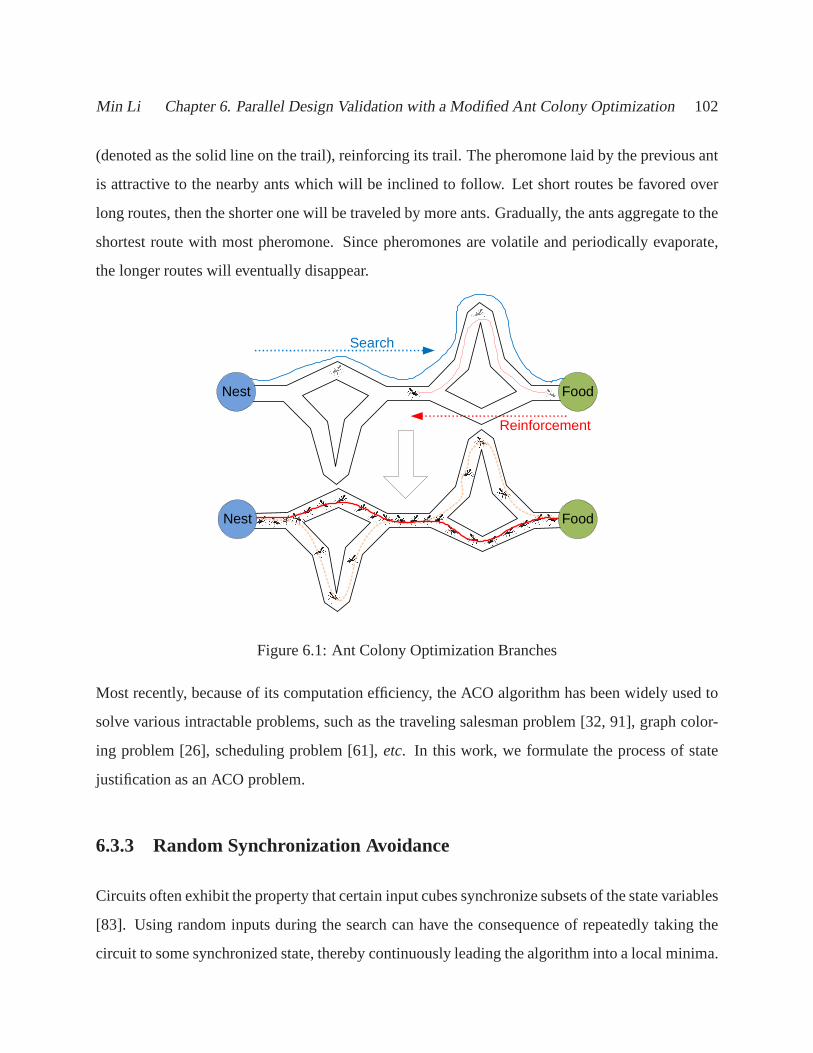
Min Li Chapter 6. Parallel Design Validation with a Modified Ant Colony Optimization 102
(denoted as the solid line on the trail), reinforcing its trail. The pheromone laid by the previous ant
is attractive to the nearby ants which will be inclined to follow. Let short routes be favored over
long routes, then the shorter one will be traveled by more ants. Gradually, the ants aggregate to the
shortest route with most pheromone. Since pheromones are volatile and periodically evaporate,
the longer routes will eventually disappear.
Search
Reinforcement
Nest Food
Nest Food
Figure 6.1: Ant Colony Optimization Branches
Most recently, because of its computation efficiency, the ACO algorithm has been widely used to
solve various intractable problems, such as the traveling salesman problem [32, 91], graph color-
ing problem [26], scheduling problem [61],etc. In this work, we formulate the process of state
justification as an ACO problem.
6.3.3 Random Synchronization Avoidance
Circuits often exhibit the property that certain input cubes synchronize subsets of the state variables
[83]. Using random inputs during the search can have the consequence of repeatedly taking the
circuit to some synchronized state, thereby continuously leading the algorithm into a local minima.
Min Li Chapter 6. Parallel Design Validation with a Modified Ant Colony Optimization 103
In order to avoid the effects of random synchronization, we have implemented an input biasing
scheme to avoid certain input cubes that potentially synchronize the state space. To check this we
simulate each primary input,wk, such thatnv is the number of flip flops initialized by assigning
a valuev to wk and simulating with otherwise unconstrained remaining input and state variables.
For each inputwk we get two values, namelyn0 andn1. Additionally, a scaling factorC is applied
to control how quickly we bias against the value. The bias against high values ofn is characterized
by the function:
P0(k) = 0.5× 0.5n0−n1
#FFs×C
P1(k) = 1.0− P0(k)
This provides a method under which the probability of a giveninput value on a PI decays based on
the difference in the number of state variables set by the given value and its complement. For use
in our experiments, we use a scaling factor ofC = 0.05 to generate bias. For example, if a PIwj
sets two FFs to 0 and one to 1, thenP0(j) = 0.5× 0.51
#FFs/20 . If the number of FFs is large,P0(j)
would be close to 0.5. On the other hand, suppose there existsa PIwk that can reset all FFs. Then,
P0(k) = 0.5× 0.520 = 0.521, a very small value.
6.4 Proposed Method
The high level flow of our algorithm is as follows: Initially,10,000 random vectors are simulated
for the construction of the partition navigation tracks. Then, random synchronization avoidance
is calculated, whose result is used to set the input bias of the GPU random input generator. Next,
the search for a vector sequence that can bring the circuit from the initial state to the target state
begins and the details will be discussed in Sections 6.4.1 and 6.4.2. If GACO finds the target state,
the Algorithm is terminated; otherwise, if GACO fails to findthe target state, the BMC described
in Section 6.4.3, is run to try to bridge the final steps to the target.
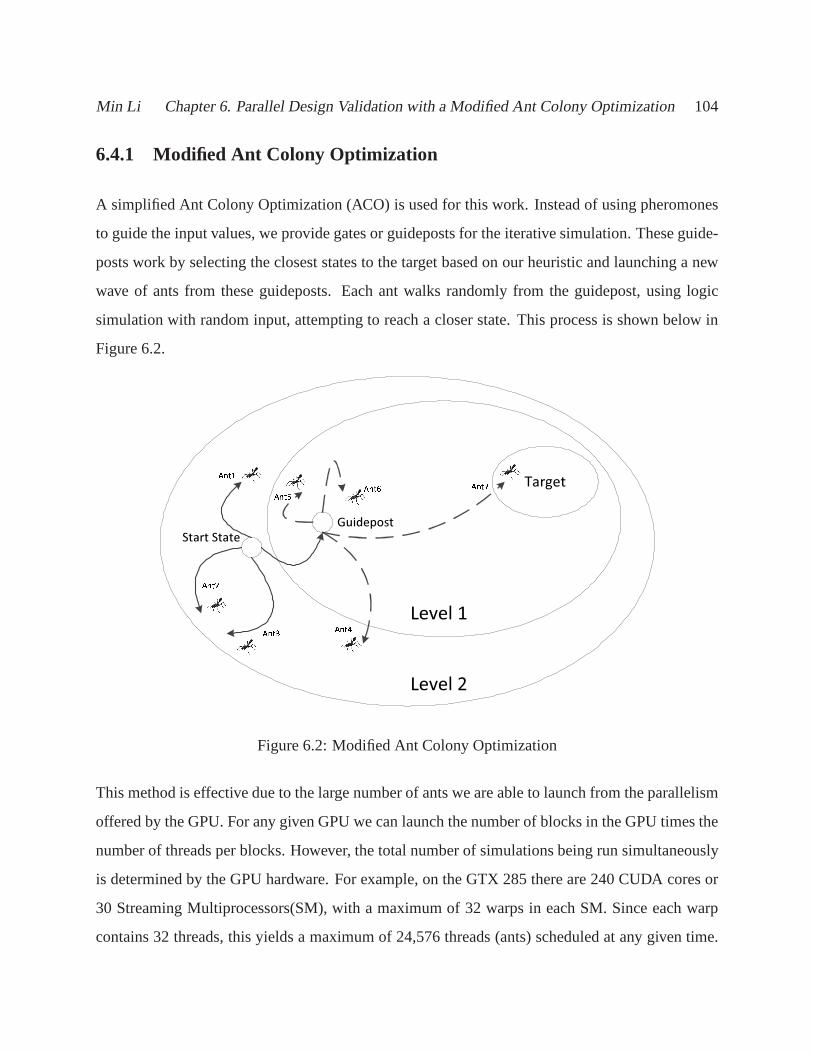
Min Li Chapter 6. Parallel Design Validation with a Modified Ant Colony Optimization 104
6.4.1 Modified Ant Colony Optimization
A simplified Ant Colony Optimization (ACO) is used for this work. Instead of using pheromones
to guide the input values, we provide gates or guideposts forthe iterative simulation. These guide-
posts work by selecting the closest states to the target based on our heuristic and launching a new
wave of ants from these guideposts. Each ant walks randomly from the guidepost, using logic
simulation with random input, attempting to reach a closer state. This process is shown below in
Figure 6.2.
Start StateStart StateGuidepostGuidepost
���������������� �������� ��������
�������� �������� ������Level 1Level 1
Level 2Level 2
TargetTarget
Figure 6.2: Modified Ant Colony Optimization
This method is effective due to the large number of ants we areable to launch from the parallelism
offered by the GPU. For any given GPU we can launch the number of blocks in the GPU times the
number of threads per blocks. However, the total number of simulations being run simultaneously
is determined by the GPU hardware. For example, on the GTX 285there are 240 CUDA cores or
30 Streaming Multiprocessors(SM), with a maximum of 32 warps in each SM. Since each warp
contains 32 threads, this yields a maximum of 24,576 threads(ants) scheduled at any given time.
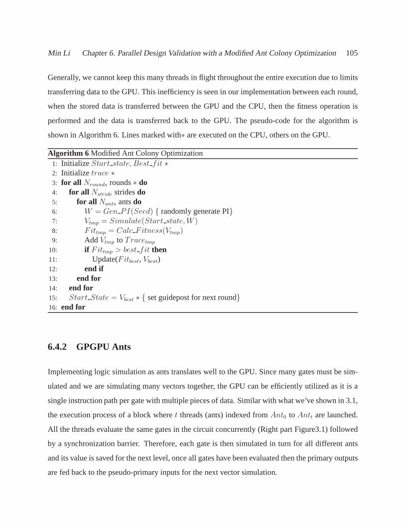
Min Li Chapter 6. Parallel Design Validation with a Modified Ant Colony Optimization 105
Generally, we cannot keep this many threads in flight throughout the entire execution due to limits
transferring data to the GPU. This inefficiency is seen in ourimplementation between each round,
when the stored data is transferred between the GPU and the CPU, then the fitness operation is
performed and the data is transferred back to the GPU. The pseudo-code for the algorithm is
shown in Algorithm 6. Lines marked with∗ are executed on the CPU, others on the GPU.
Algorithm 6 Modified Ant Colony Optimization1: Initialize Start state, Best fit ∗2: Initialize trace ∗3: for all Nrounds rounds∗ do4: for all Nstride stridesdo5: for all Nants antsdo6: W = Gen PI(Seed) { randomly generate PI}7: Vtmp = Simulate(Start state,W )8: Fittmp = Calc F itness(Vtmp)9: Add Vtmp to Tracetmp
10: if Fittmp > best fit then11: Update(Fitbest, Vbest)12: end if13: end for14: end for15: Start State = Vbest ∗ { set guidepost for next round}16: end for
6.4.2 GPGPU Ants
Implementing logic simulation as ants translates well to the GPU. Since many gates must be sim-
ulated and we are simulating many vectors together, the GPU can be efficiently utilized as it is a
single instruction path per gate with multiple pieces of data. Similar with what we’ve shown in 3.1,
the execution process of a block wheret threads (ants) indexed fromAnt0 to Antt are launched.
All the threads evaluate the same gates in the circuit concurrently (Right part Figure3.1) followed
by a synchronization barrier. Therefore, each gate is then simulated in turn for all different ants
and its value is saved for the next level, once all gates have been evaluated then the primary outputs
are fed back to the pseudo-primary inputs for the next vectorsimulation.
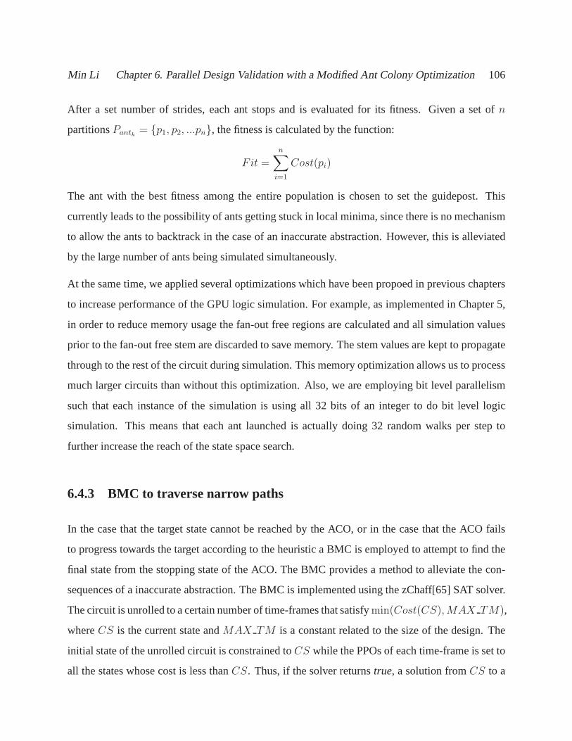
Min Li Chapter 6. Parallel Design Validation with a Modified Ant Colony Optimization 106
After a set number of strides, each ant stops and is evaluatedfor its fitness. Given a set ofn
partitionsPantk = {p1, p2, ...pn}, the fitness is calculated by the function:
Fit =
n∑
i=1
Cost(pi)
The ant with the best fitness among the entire population is chosen to set the guidepost. This
currently leads to the possibility of ants getting stuck in local minima, since there is no mechanism
to allow the ants to backtrack in the case of an inaccurate abstraction. However, this is alleviated
by the large number of ants being simulated simultaneously.
At the same time, we applied several optimizations which have been propoed in previous chapters
to increase performance of the GPU logic simulation. For example, as implemented in Chapter 5,
in order to reduce memory usage the fan-out free regions are calculated and all simulation values
prior to the fan-out free stem are discarded to save memory. The stem values are kept to propagate
through to the rest of the circuit during simulation. This memory optimization allows us to process
much larger circuits than without this optimization. Also,we are employing bit level parallelism
such that each instance of the simulation is using all 32 bitsof an integer to do bit level logic
simulation. This means that each ant launched is actually doing 32 random walks per step to
further increase the reach of the state space search.
6.4.3 BMC to traverse narrow paths
In the case that the target state cannot be reached by the ACO,or in the case that the ACO fails
to progress towards the target according to the heuristic a BMC is employed to attempt to find the
final state from the stopping state of the ACO. The BMC provides a method to alleviate the con-
sequences of a inaccurate abstraction. The BMC is implemented using the zChaff[65] SAT solver.
The circuit is unrolled to a certain number of time-frames that satisfymin(Cost(CS),MAX TM),
whereCS is the current state andMAX TM is a constant related to the size of the design. The
initial state of the unrolled circuit is constrained toCS while the PPOs of each time-frame is set to
all the states whose cost is less thanCS. Thus, if the solver returnstrue, a solution fromCS to a
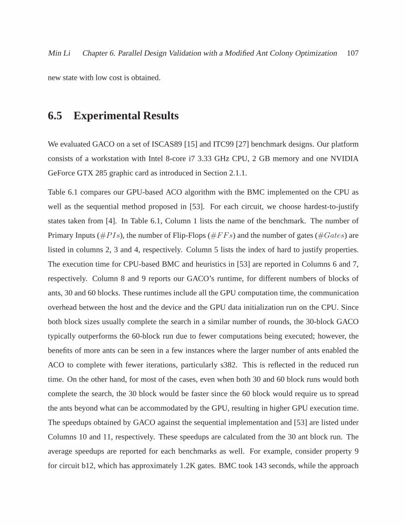
Min Li Chapter 6. Parallel Design Validation with a Modified Ant Colony Optimization 107
new state with low cost is obtained.
6.5 Experimental Results
We evaluated GACO on a set of ISCAS89 [15] and ITC99 [27] benchmark designs. Our platform
consists of a workstation with Intel 8-core i7 3.33 GHz CPU, 2GB memory and one NVIDIA
GeForce GTX 285 graphic card as introduced in Section 2.1.1.
Table 6.1 compares our GPU-based ACO algorithm with the BMC implemented on the CPU as
well as the sequential method proposed in [53]. For each circuit, we choose hardest-to-justify
states taken from [4]. In Table 6.1, Column 1 lists the name ofthe benchmark. The number of
Primary Inputs (#PIs), the number of Flip-Flops (#FFs) and the number of gates (#Gates) are
listed in columns 2, 3 and 4, respectively. Column 5 lists theindex of hard to justify properties.
The execution time for CPU-based BMC and heuristics in [53] are reported in Columns 6 and 7,
respectively. Column 8 and 9 reports our GACO’s runtime, fordifferent numbers of blocks of
ants, 30 and 60 blocks. These runtimes include all the GPU computation time, the communication
overhead between the host and the device and the GPU data initialization run on the CPU. Since
both block sizes usually complete the search in a similar number of rounds, the 30-block GACO
typically outperforms the 60-block run due to fewer computations being executed; however, the
benefits of more ants can be seen in a few instances where the larger number of ants enabled the
ACO to complete with fewer iterations, particularly s382. This is reflected in the reduced run
time. On the other hand, for most of the cases, even when both 30 and 60 block runs would both
complete the search, the 30 block would be faster since the 60block would require us to spread
the ants beyond what can be accommodated by the GPU, resulting in higher GPU execution time.
The speedups obtained by GACO against the sequential implementation and [53] are listed under
Columns 10 and 11, respectively. These speedups are calculated from the 30 ant block run. The
average speedups are reported for each benchmarks as well. For example, consider property 9
for circuit b12, which has approximately 1.2K gates. BMC took 143 seconds, while the approach
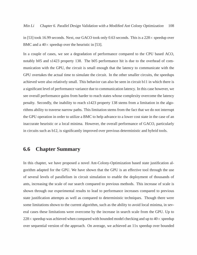
Min Li Chapter 6. Parallel Design Validation with a Modified Ant Colony Optimization 108
in [53] took 16.99 seconds. Next, our GACO took only 0.63 seconds. This is a 228× speedup over
BMC and a 40× speedup over the heuristic in [53].
In a couple of cases, we see a degradation of performance compared to the CPU based ACO,
notably b05 and s1423 property 138. The b05 performance hit is due to the overhead of com-
munication with the GPU, the circuit is small enough that thelatency to communicate with the
GPU overtakes the actual time to simulate the circuit. In theother smaller circuits, the speedups
achieved were also relatively small. This behavior can alsobe seen in circuit b11 in which there is
a significant level of performance variance due to communication latency. In this case however, we
see overall performance gains from harder to reach states whose complexity overcome the latency
penalty. Secondly, the inability to reach s1423 property 138 stems from a limitation in the algo-
rithms ability to traverse narrow paths. This limitation stems from the fact that we do not interrupt
the GPU operation in order to utilize a BMC to help advance to alower cost state in the case of an
inaccurate heuristic or a local minima. However, the overall performance of GACO, particularly
in circuits such as b12, is significantly improved over previous deterministic and hybrid tools.
6.6 Chapter Summary
In this chapter, we have proposed a novel Ant-Colony-Optimization based state justification al-
gorithm adapted for the GPU. We have shown that the GPU is an effective tool through the use
of several levels of parallelism in circuit simulation to enable the deployment of thousands of
ants, increasing the scale of our search compared to previous methods. This increase of scale is
shown through our experimental results to lead to performance increases compared to previous
state justification attempts as well as compared to deterministic techniques. Though there were
some limitations shown to the current algorithm, such as theability to avoid local minima, in sev-
eral cases these limitations were overcome by the increase in search scale from the GPU. Up to
228× speedup was achieved when compared with bounded model checking and up to 40× speedup
over sequential version of the approach. On average, we achieved an 11x speedup over bounded
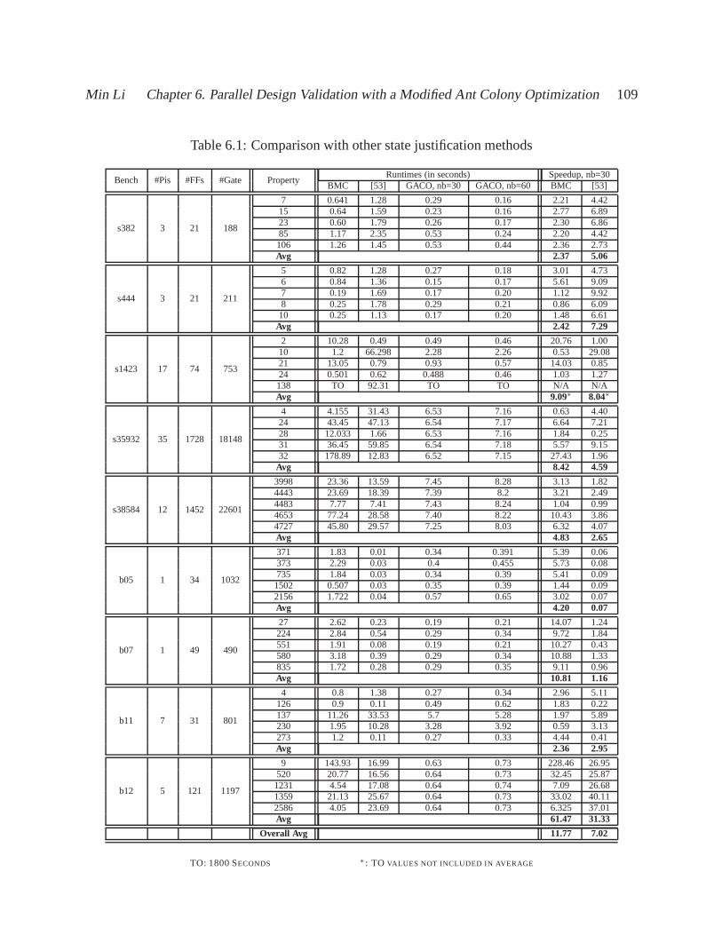
Min Li Chapter 6. Parallel Design Validation with a Modified Ant Colony Optimization 109
Table 6.1: Comparison with other state justification methods
Bench #Pis #FFs #Gate PropertyRuntimes (in seconds) Speedup, nb=30
BMC [53] GACO, nb=30 GACO, nb=60 BMC [53]
s382 3 21 188
7 0.641 1.28 0.29 0.16 2.21 4.4215 0.64 1.59 0.23 0.16 2.77 6.8923 0.60 1.79 0.26 0.17 2.30 6.8685 1.17 2.35 0.53 0.24 2.20 4.42106 1.26 1.45 0.53 0.44 2.36 2.73Avg 2.37 5.06
s444 3 21 211
5 0.82 1.28 0.27 0.18 3.01 4.736 0.84 1.36 0.15 0.17 5.61 9.097 0.19 1.69 0.17 0.20 1.12 9.928 0.25 1.78 0.29 0.21 0.86 6.0910 0.25 1.13 0.17 0.20 1.48 6.61
Avg 2.42 7.29
s1423 17 74 753
2 10.28 0.49 0.49 0.46 20.76 1.0010 1.2 66.298 2.28 2.26 0.53 29.0821 13.05 0.79 0.93 0.57 14.03 0.8524 0.501 0.62 0.488 0.46 1.03 1.27138 TO 92.31 TO TO N/A N/AAvg 9.09∗ 8.04∗
s35932 35 1728 18148
4 4.155 31.43 6.53 7.16 0.63 4.4024 43.45 47.13 6.54 7.17 6.64 7.2128 12.033 1.66 6.53 7.16 1.84 0.2531 36.45 59.85 6.54 7.18 5.57 9.1532 178.89 12.83 6.52 7.15 27.43 1.96
Avg 8.42 4.59
s38584 12 1452 22601
3998 23.36 13.59 7.45 8.28 3.13 1.824443 23.69 18.39 7.39 8.2 3.21 2.494483 7.77 7.41 7.43 8.24 1.04 0.994653 77.24 28.58 7.40 8.22 10.43 3.864727 45.80 29.57 7.25 8.03 6.32 4.07Avg 4.83 2.65
b05 1 34 1032
371 1.83 0.01 0.34 0.391 5.39 0.06373 2.29 0.03 0.4 0.455 5.73 0.08735 1.84 0.03 0.34 0.39 5.41 0.091502 0.507 0.03 0.35 0.39 1.44 0.092156 1.722 0.04 0.57 0.65 3.02 0.07Avg 4.20 0.07
b07 1 49 490
27 2.62 0.23 0.19 0.21 14.07 1.24224 2.84 0.54 0.29 0.34 9.72 1.84551 1.91 0.08 0.19 0.21 10.27 0.43580 3.18 0.39 0.29 0.34 10.88 1.33835 1.72 0.28 0.29 0.35 9.11 0.96Avg 10.81 1.16
b11 7 31 801
4 0.8 1.38 0.27 0.34 2.96 5.11126 0.9 0.11 0.49 0.62 1.83 0.22137 11.26 33.53 5.7 5.28 1.97 5.89230 1.95 10.28 3.28 3.92 0.59 3.13273 1.2 0.11 0.27 0.33 4.44 0.41Avg 2.36 2.95
b12 5 121 1197
9 143.93 16.99 0.63 0.73 228.46 26.95520 20.77 16.56 0.64 0.73 32.45 25.871231 4.54 17.08 0.64 0.74 7.09 26.681359 21.13 25.67 0.64 0.73 33.02 40.112586 4.05 23.69 0.64 0.73 6.325 37.01Avg 61.47 31.33
Overall Avg 11.77 7.02
TO: 1800 SECONDS ∗ : TO VALUES NOT INCLUDED IN AVERAGE

Min Li Chapter 6. Parallel Design Validation with a Modified Ant Colony Optimization 110
model checking and a 7x speedup compared to the sequential approach.
Chapter 7
Conclusion
In this dissertation, we addressed several GPU based applications within two topics: digital sys-
tems testing and validation. For testing area, we proposed efficient logic fault simulation, fault-
diagnostic simulation and reliability analysis on GPUs. Totackle state justification which is one of
the most difficult design validation problems, we introduced a parallel abstraction-guided search
scheme using ant colony optimization. All the proposed GPU-based applications aim at accelerat-
ing the EDA tools and hence improving the design flow of digital systems.
In Chapter 3, we presented an efficient parallel fault simulator with GPGPU, called FSimGP2. We
proposed a three dimensional parallelism, namelyPattern-parallelism, cf-parallelismandBlock-
parallelismto achieve a high algorithmic efficiency on GPUs. A large number of gate evaluations
can be performed in parallel by employing the large number ofthreads on a GPU. Fault injection is
preformed in a novel compact-fault style which helps to achieve a speedup of 3×. The CUDA run-
ning hierarchy is also exploited as block-parallelism which utilizes the high computational power
of the many-core system. Experimental results showed that FSimGP2 could achieve an average
of 25.576× and 3.606× speedup when compared with two previous GPU-based fault simulators.
Moreover, FSimGP2 is also 35.168× faster, on average, than a state-of-the-art sequential fault
simulator, with a maximal speedup of more than 95×.
111
Min Li Chapter 7. Conclusion 112
We proposed a high-performance parallel fault diagnostic simulator in chapter 4. A novel idea of
multi-fault-signature (MFS) is designed for parallelism on GPUs where a number of fault signa-
tures are recorded during parallel fault simulation without introducing much overhead. Fault-pair
based diagnostic simulation is also parallelized on GPU. The proposed dynamic load balancing
approach results in an efficient utilization of the available computational resources. Experimen-
tal results showed that GDSim could achieve an average of 38× speedup when compared with a
state-of-the-art sequential fault diagnostic simulator.Moreover, GDSim is also 95× faster than its
sequential implementation based on conventional processor architectures.
In Chapter 5, we implemented RAG, which is the first GPU-basedreliability analysis tool for logic
circuits. The initial barrier to achieve high degree of parallelism is that some large benchmarks
cannot be fitted into the global memory of GPUs because all thefault-free and faulty logic values
are necessary to store on-board. Novel algorithms including stems scheduling and post-order tree
traversal for non-stem gates arrangement are proposed which allow for an efficient utilization of
the available computational resources on the GPU. Experimental results showed that RAG could
achieve an average of 353× and 116× speedup against two state-of-the-art reliability analysis
tools.
In the area of design validation, our ACO-based approach formulates state justification as a path
search problem, where artificial ants, starting from their nest (the initial state), attempt to find the
paths to food (the target state). We exploited the swarm intelligence to efficiently guide the search
which takes advantage of the collective behavior from a colony of ants and can effectively avoid
some critical local optimal points during the search. Furthermore, the simulation-based nature
of the approach avoids memory explosion often faced by formal techniques. Also, we used our
existed GPU framework to achieve several levels of parallelism in circuit simulation and is enable
the deployment of thousands of ants, increasing the scale ofour search compared to previous
methods.
In sum, we chose several applications for which there is a strong motivation to accelerate, since
they are extensively used in the VLSI design flow. We implemented varied degrees of inherent
Min Li Chapter 7. Conclusion 113
parallelism in them and achieved more than one magnitude speed-up against other tools on the
conventional CPU architectures and the GPU systems as well.We believe that the approaches and
ideas we proposed for acceleration on GPUs could also be applied to other applications in not only
EDA area but also other fields.
Chapter 8
Bibliography
[1] A. Abdollahi. Probabilistic decision diagrams for exact probabilistic analysis. InProc. Int.
Conf. Computer-Aided Design, pages 266–272, 2007.
[2] M. Abramovici, M. Breuer, A. Friedman, I. of Electrical,and E. Engineers.Digital systems
testing and testable design. IEEE press New York, 1990.
[3] M. Abramovici, Y. H. Levendel, and P. R. Menon. A logic simulation machine. InProc.
Int. Symp. Computer Architecture, pages 148–157, 1982.
[4] State justification benchmarks.http://filebox.vt.edu/users/minli/Web/
state_just.html.
[5] P. Agrawal, W. J. Dally, and W. C. F.et al. MARS: A multiprocessor-based programmable
accelerator.IEEE Des. Test Comput., pages 28–36, 1987.
[6] M. B. Amin and B. Vinnakota. Data parallel fault simulation. InProc. Int. Conf. Computer
Design, pages 610–615, 1995.
[7] M. B. Amin and B. Vinnakota. Workload distribution in fault simulation. J. Electronic
Testing: Theory and Applicat., 10(3):277–282, 1997.
114
Min Li Bibliography 115
[8] R. I. Bahar, J. Mundy, and J. Chen. A probabilistic-baseddesign methodology for nanoscale
computation. InProc. Int. Conf. Computer-Aided Design, 2003.
[9] S. Bai and D. Nicol. Gpu coprocessing for wireless network simulation. Technical report,
Technical Report, University of Illinois at Urbana-Champaign, 2008.
[10] D. K. Beece, G. Deiberg, G. Papp, and F. Villante. The IBMengineering verification engine.
In Proc. Design Automation Conf., pages 218–224, 1988.
[11] G. E. Blelloch. Vector models for data-parallel computing. MIT Press, Cambridge, MA,
USA, 1990.
[12] V. Boppana, S. Rajan, K. Takayama, and M. Fujita. Model checking based on sequential
ATPG. InProc. Int. Conf. Computer-Aided Verification, pages 418–430, 1999.
[13] G. Bourianoff. The future of nanocomputing.Computer, pages 44–53, 2003.
[14] M. A. Breuer, S. K. Gupta, and T. Mak. Defect and error tolerance in the presence of massive
numbers of defects.IEEE Des. Test Comput., 21(3):216–227, 2004.
[15] F. Brglez, D. Bryan, and K. Kozminski. Combinational profiles of sequential benchmark
circuits. InProc. Int. Symp. Circuits & Systems, pages 1929–1934, 1989.
[16] J. Burch, E. Clarke, K. McMillan, D. Dill, and L. Hwang. Symbolic model checking:1020
states and beyond. InLogic in Computer Science, 1990. LICS ’90, Proceedings., Fifth
Annual IEEE Symposium, pages 428–439, jun 1990.
[17] P. Camurati, D. Medina, P. Prinetto, and M. R. Sonza. A diagnostic test pattern generation
algorithm. InProc. Int. Test Conf., pages 52–58, 1990.
[18] G. R. Case. Analysis of actual fault mechanisms in cmos logic gates. InProceedings of the
13th Design Automation Conference, DAC ’76, pages 265–270, New York, NY, USA, 1976.
ACM.
Min Li Bibliography 116
[19] S. Chakravarty, Y. Gong, and S. Venkataraman. Diagnostic simulation of stuck-at faults in
combinational circuits.J. Electronic Testing: Theory and Applicat., 8(1):87–97, 1996.
[20] D. Chatterjee, A. DeOrio, and V. Bertacco. Event-driven gate-level simulation with gp-gpus.
In Proc. Design Automation Conf., pages 557–562, 2009.
[21] D. Chatterjee, A. DeOrio, and V. Bertacco. GCS: High-performance gate-level simulation
with gpgpus. InProc. Design Automation & Test Europe Conf., pages 1332–1337, 2009.
[22] H. Chen and J. Han. Stochastic computational models foraccurate reliability evaluation of
logic circuits. InProc. Great Lake Symp. VLSI, pages 61–66, 2010.
[23] S. C. Chen and J. M. Jou. Diagnostic fault simulation forsynchronous sequential circuits.
IEEE Trans. Comput.-Aided Des. Integr. Circuits Syst., 16(3):299–308, 1997.
[24] M. R. Choudhury and K. Mohanram. Reliability analysis of logic circuits. IEEE Trans.
Comput.-Aided Des. Integr. Circuits Syst., 28(3):392–405, 2009.
[25] E. Clarke, O. Grumberg, and D. Peled. Model checking, 2000.
[26] D. Costa and A. Hertz. Ants can colour graphs.J. Operational Research Society, 48(3):295–
305, 1997.
[27] S. Davidson. ITC99 benchmark circuits - preliminary results. InProc. Int. Symp. Circuits
& Systems, page 1125, 1999.
[28] F. De Paula and A. Hu. An effective guidance strategy forabstraction-guided simulation. In
Proc. Design Automation Conf., pages 63–68, june 2007.
[29] Y. Deng, B. Wang, and S. Mu. Taming irregular eda applications on gpus. InProc. Design
Automation Conf., pages 539–546, Nov. 2009.
[30] M. Dorigo. Optimization, learning and natural algorithms. PhD thesis, Politecnico di
Milano, 1995.
Min Li Bibliography 117
[31] M. Dorigo, M. Birattari, and T. Stutzle. Ant colony optimization artificial ants as a compu-
tational intelligence technique.IEEE Computer Intelligence Magazine, 1(4):28–39, 2006.
[32] M. Dorigo, V. Maniezzo, and A. Colorni. Ant system: Optimization by a colony of cooper-
ating agents.IEEE Tran. Systems, Man, and Cybernetics, 26(1):29–41, Feb 1996.
[33] Z. Fan, F. Qiu, A. Kaufman, and S. Yoakum-Stover. Gpu cluster for high performance
computing. InProceedings of the 2004 ACM/IEEE conference on Supercomputing, SC ’04,
pages 47–, Washington, DC, USA, 2004. IEEE Computer Society.
[34] G. D. P. Flavio and A. J. Hu. An effective guidance strategy for abstraction-guided simula-
tion. In Proc. Design Automation Conf., pages 63–68, 2007.
[35] M. K. Ganai, A. Aziz, and A. Kuehlmann. Enhancing simulation with BDDs and ATPG. In
Proc. Design Automation Conf., pages 385–390, 1999.
[36] T. Godjoska, S. Filiposka, and D. Trajanov. Parallel execution of the ns-2 sequential sim-
ulator on a gpu. In18th Telecommunications forum TELFOR 2010, pages 159–162, Nov.
2010.
[37] N. K. Govindaraju, N. Raghuvanshi, and D. Manocha. Fastand approximate stream mining
of quantiles and frequencies using graphics processors. InProceedings of the 2005 ACM
SIGMOD international conference on Management of data, SIGMOD ’05, pages 611–622,
New York, NY, USA, 2005.
[38] K. Gulati and S. Khatri. Towards acceleration of fault simulation using graphics processing
units. InProc. Design Automation Conf., pages 822–827, 2008.
[39] K. Gulati and S. P. Khatri. Fault Table Computation on GPUs. J. Electronic Testing: Theory
and Applicat., 26(2):195–209, 2010.
[40] I. Hamzaoglu and J. H. Patel. New techniques for deterministic test pattern generation. In
J. Electronic Testing: Theory and Applicat., pages 446–452, 1999.
Min Li Bibliography 118
[41] J. Han, E. Taylor, J. Gao, and J. Fortes. Faults, Error Bounds and Reliability of Nanoelec-
tronic Circuits. InProc. Int. Conf. Appl.-Specific Sys., Arch. and Proc., pages 247–253,
2005.
[42] S. Han, K. Jang, K. Park, and S. Moon. Packetshader: a gpu-accelerated software router.
SIGCOMM Comput. Commun. Rev., 41:195–206, Aug. 2010.
[43] N. Ishiura, M. Ito, and S. Yajima. Dynamic two-dimensional parallel simulation technique
for high-speed fault simulation on a vector processor.IEEE Trans. Comput.-Aided Des.
Integr. Circuits Syst., 9(8):868–875, aug 1990.
[44] IWLS 2005 benchmarks. http://www.iwls.org/iwls2005/benchmarks.
html.
[45] R. W. Keyes. Fundamental limits of silicon technology.Proceedings of the IEEE,
89(3):227–239, 2001.
[46] Y. Kitamura. Exact critical path tracing fault simulation on massively parallel processor
AAP2. In Proc. Int. Conf. Computer-Aided Design, pages 474–477, 1989.
[47] M. A. Kochte, M. Schaal, H. J. Wunderlich, and C. G. Zoellin. Efficient fault simulation on
many-core processors. InProc. Design Automation Conf., pages 380–385, 2010.
[48] S. Krishnaswamy, G. Viamontes, I. Markov, and J. Hayes.Accurate reliability evaluation
and enhancement via probabilistic transfer matrices. InProc. Design Automation & Test
Europe Conf., pages 282–287, 2005.
[49] S. Krishnaswamy, G. F. Viamontes, I. L. Markov, and J. P.Hayes. Probabilistic transfer
matrices in symbolic reliability analysis of logic circuits. ACM Trans. Design Automation
Electronic Systems, 13(1):1–35, 2008.
[50] K. Kubiak, S. Parkes, W. K. Fuchs, and R. Saleh. Exact evaluation of diagnostic test reso-
lution. In Proc. Design Automation Conf., pages 347–352, 1992.
Min Li Bibliography 119
[51] K. Lee and D. Ha. An efficient, forward fault simulation algorithm based on the parallel
pattern single fault propagation. InProc. Int. Test Conf., pages 946–955, 1991.
[52] M. Li, K. Gent, and M. S. Hsiao. Utilizing gpgpus for design validation with a modified ant
colony optimization. InProceedings of the High-Level Design Validation and Test Work-
shop, pages 128–135. IEEE Computer Society, 2011.
[53] M. Li and M. S. Hsiao. An ant colony optimization technique for abstraction-guided state
justification. InProc. Int. Test Conf., pages 1–10, 2009.
[54] M. Li and M. S. Hsiao. FsimGP2: An efficient fault simulator with GPGPU. InProc. Asian
Test Symp., pages 15–20, 2010.
[55] M. Li and M. S. Hsiao. 3-d parallel fault simulation withgpgpu.IEEE Trans. Comput.-Aided
Des. Integr. Circuits Syst., 30(10):1545–1555, Oct. 2011.
[56] M. Li and M. S. Hsiao. High-performance diagnostic fault simulation on gpus. InProc.
European Test Symp., page 210, May 2011.
[57] M. Li and M. S. Hsiao. RAG: an efficient reliability analysis of logic circuits on graphics
processing units. InProc. Design Automation & Test Europe Conf., pages 316–319, 2012.
[58] M. Li, Y. Zheng, M. S. Hsiao, and C. Huang. Reversible logic synthesis through ant colony
optimization. InProc. Design Automation & Test Europe Conf., pages 307–310, 2010.
[59] E. Lindholm, J. Nickolls, and J. M. S. Oberman. NVIDIA Tesla: A unified graphics and
computing architecture.IEEE Micro, 28(2):39–55, 2008.
[60] D. Luebke, M. Harris, J. Kruger, T. Purcell, N. Govindaraju, I. Buck, C. Woolley, and
A. Lefohn. Gpgpu: general purpose computation on graphics hardware. InACM SIG-
GRAPH 2004 Course Notes, SIGGRAPH ’04, New York, NY, USA, 2004. ACM.
[61] S. Luo, C. Wang, and J. Wang. Ant colony optimization forresource-constrained project
scheduling with generalized precedence relations. InIEEE Proc. Tools with Artificial Intel-
ligence, pages 284–289, Nov. 2003.
Min Li Bibliography 120
[62] S. Manavski. Cuda compatible gpu as an efficient hardware accelerator for aes cryptography.
In IEEE International Conference on Signal Processing and Communications, pages 65–68,
Nov. 2007.
[63] J. D. Meindl, Q. Chen, and J. A. Davis. Limits on silicon nanoelectronics for terascale
integration.Science, 293(5537):2044, 2001.
[64] G. Moore. Cramming more components onto integrated circuits. Proceedings of the IEEE,
86(1):82–85, 1998.
[65] M. Moskewicz, C. Madigan, Y. Zhao, L. Zhang, and S. Malik. Chaff: engineering an
efficient sat solver. InProc. Design Automation Conf., pages 530–535, 2001.
[66] R. B. Mueller-Thuns, D. G. Saab, and R. F. D. J. A. Abraham. VLSI logic and fault sim-
ulation on general-purpose parallel computers.IEEE Trans. Comput.-Aided Des. Integr.
Circuits Syst., 12(3):446–460, 1993.
[67] M. Nanjundappa, H. Patel, B. Jose, and S. Shukla. Scgpsim: A fast systemc simulator on
gpus. InProc. Asia South Pacific Design Automation Conf., pages 149–154, Jan. 2010.
[68] K. Nanshi and F. Somenzi. Guiding simulation with increasingly refined abstract traces. In
Proc. Design Automation Conf., pages 737–742, 2006.
[69] V. Narayanan and V. Pitchumani. Fault simulation on massively parallel SIMD machines al-
gorithms, implementations and results.J. Electronic Testing: Theory and Applicat., 3(1):79–
92, 1992.
[70] T. Niermann and J. H. Patel. HITEC: a test generation package for sequential circuits. In
Proc. Design Automation & Test Europe Conf., pages 214–218, 1991.
[71] T. M. Niermann, W. T. Cheng, and J. H. Patel. PROOFS: A fast, memory-efficient sequential
circuit fault simulator.IEEE Trans. Comput.-Aided Des. Integr. Circuits Syst., 11(2):198–
207, 1992.
Min Li Bibliography 121
[72] NVIDIA CUDA homepage. http://www.nvidia.com/object/cuda_home.
html.
[73] NVIDIA Tesla Data Center Solutions. http://www.nvidia.com/object/
preconfigured-clusters.html.
[74] J. Owens, M. Houston, D. Luebke, S. Green, J. Stone, and J. Phillips. Gpu computing.
Proceedings of the IEEE, 96(5):879–899, May 2008.
[75] J. Owens, D. Luebke, N. Govindaraju, M. Harris, J. Kruger, A. Lefohn, and T. Purcell. A
survey of general-purpose computation on graphics hardware. Computer graphics forum,
26(1):80–113, 2007.
[76] F. Ozguner, C. Aykanat, and O. Khalid. Logic fault simulation on a vector hypercube multi-
processor. InProc. Conf. Hypercube Concurrent Computer and Applications, pages 1108–
1116, 1988.
[77] F. Ozguner and R. Daoud. Vectorized fault simulation onthe Cray X-MP supercomputer.
In Proc. Int. Conf. Computer-Aided Design, pages 198–201, 1988.
[78] A. Parikh, W. Wu, and M. Hsiao. Mining-guided state justification with partitioned nav-
igation tracks. InTest Conference, 2007. ITC 2007. IEEE International, pages 1–10, oct.
2007.
[79] S. Parkes, P. Banerjee, and J. Patel. A parallel algorithm for fault simulation based on
PROOFS. InProc. Int. Conf. Computer Design, pages 616–621, 1995.
[80] S. Patil and P. Banerjee. Performance trade-offs in a parallel test generation/fault simulation
environment. IEEE Trans. Comput.-Aided Des. Integr. Circuits Syst., 10(12):1542–1558,
1991.
[81] M. Pharr and R. Fernando.GPU Gems 2: Programming Techniques for High-performance
Graphics and General-Purpose Computation. Addison-Wesley Professional, 2005.
Min Li Bibliography 122
[82] I. Pomeranz. On pass/fail dictionaries for scan circuits. In Proc. Asian Test Symp., pages
51–56, 2001.
[83] I. Pomeranz and S. Reddy. Primary input vectors to avoidin random test sequences for
synchronous sequential circuits.Proc. Int. Conf. Computer-Aided Design, 27(1):193–197,
Jan. 2008.
[84] R. Raghavan, J. P. Hayes, and W. R. Martin. Logic simulation on vector processors. InProc.
Int. Conf. Computer-Aided Design, pages 268–271, 1988.
[85] P. Rashinkar, P. Paterson, and L. Singh.System-on-a-chip verification: methodology and
techniques. Springer Netherlands, 2000.
[86] T. Rejimon and S. Bhanja. Scalable probabilistic computing models using Bayesian net-
works. InProc. Int. Symp. Circuits & Systems, pages 712–715, 2005.
[87] E. M. Rudnick, T. M. Niermann, and J. H. Patel. Methods for reducing events in sequential
circuit fault simulation. InProc. Int. Conf. Computer-Aided Design, pages 546–549, 1991.
[88] A. Santone. Heuristic search + local model checking in selective mu-calculus.Software
Engineering, IEEE Transactions on, 29(6):510–523, June 2003.
[89] J. Shen, W. Maly, and F. Ferguson. Inductive fault analysis of mos integrated circuits.
Design Test of Computers, IEEE, 2(6):13–26, Dec. 1985.
[90] S. Shyam and V. Bertacco. Distance-guided hybrid verification with GUIDO. InProc.
Design Automation Conf., volume 1, pages 1–6, march 2006.
[91] T. Stutzle and H. Hoos. Max-min ant system and local search for the traveling salesman
problem. InIEEE Int. Conf. Evolutionary Computation, pages 309–314, Apr 1997.
[92] R. Szerwinski and T. Gneysu. Exploiting the power of gpus for asymmetric cryptography. In
Cryptographic Hardware and Embedded Systems CHES 2008, volume 5154, pages 79–99.
Springer Berlin / Heidelberg, 2008.
Min Li Bibliography 123
[93] S. Tai and D. Bhattacharya. Pipelined fault simulationon parallel machines using the circuit
flow graph. InProc. Int. Conf. Computer Design, pages 564–567, 1993.
[94] E. Taylor, J. Han, and J. Fortes. Towards accurate and efficient reliability modeling of
nanoelectronic circuits. InProc. IEEE Conf. Nanotechnology, volume 1, pages 395–398,
2006.
[95] C. Timoc, M. Buehler, T. Griswold, C. Pina, F. Stott, andL. Hess. Logical models of
physical failures. InProc. Int. Test Conf., pages 546–553. IEEE Computer Society, 1983.
[96] J. A. Van Meel, A. Arnold, and D. Frenkel. Harvesting graphics power for MD simulations.
Molecular Simulation, 34(3):259–266, 2008.
[97] J. Waicukauski and E. Lindbloom. Failure diagnosis of structured vlsi. IEEE Design and
Test of Computers, pages 49–60, 1989.
[98] Q. W. Wu and M. S. Hsiao. State variable extraction to reduce problem complexity for atpg
and design validation. InProc. Int. Test Conf., pages 820–899, 2004.
[99] C. Yang and D. Dill. Validation with guided search of thestate space. InProc. Design
Automation Conf., pages 599–604, June 1998.
[100] V. V. Zhirnov, R. K. Cavin III, J. A. Hutchby, and G. I. Bourianoff. Limits to binary logic
switch scaling-a gedanken model.Proceedings of the IEEE, 91(11):1934–1939, 2003.
Recommended