DEPARTMENT OF ENERGY TECHNOLOGY
CONDUCTED BY GROUP WPS4 - 1050
SPRING SEMESTER 2011
ACCELERATED LIFE TESTING AND LIFE
PREDICTION OF LITHIUION BATTERIES
CONNECTED TO WIND TURBINE
STUDENT REPORT
DEPARTMENT OF ENERGY TECHNOLOGY
CONDUCTED BY GROUP 1050
SPRING SEMESTER 2011
CELERATED LIFE TESTING AND LIFETIME
PREDICTION OF LITHIUM ION BATTERIES
CONNECTED TO WIND
TUDENT REPORT


3
Title: Accelerated life testing and life-time prediction of Lithium Ion
batteries connected to Wind Turbine
Semester: 10th
Semester theme: Master Thesis
Project period: 7th February – 31st May 2011
ECTS: 30
Supervisors: Remus Teodorescu
Maciej Swierczynski
Project group: WPS4 - 1050
_____________________________________
Daniel Díaz González
_____________________________________
Robert Diosi
Copies: 3
Pages, total: 99
Appendices: 3
Supplements: CD
By signing this document, each member of the group confirms that all
participated in the project work and thereby that all members are collectively liable
for the content of the report
SYNOPSIS:
The future plans regarding the increase of the
share of wind power in the Electrical Grid point out towards
major challenges that this wind power integration implies:
the need to transform the current wind parks into reliable
power generation units, capable of providing the base load,
covered by conventional generation units, at the moment.
The major obstacle in the way of a high scale wind
integration into the Grid is represented by the unpredictable
behavior of the wind.
A solution to diminish the wind power units
dependability upon the wind unpredictability can be
represented by Battery Energy Storage Systems (BES). One of
the most important requirements for a fruitful BES
integration into Wind Power Systems is a correct estimation
of their lifetime.
The present work is focused on the lifetime
estimation of Lithium Iron Phosphate cells, by applying two
accelerating factors: high temperatures and high current
rates. The laboratory work was performed by applying to the
testing setup a state of charge (SOC) input signal
corresponding to the simulation of the Forecast
Improvement Service in Simulink. The input SOC contained
data corresponding to 1 entire year of simulations. Two
groups of LiFePO4 were tested at 50 and 40 °C, respectively
and at an applied current rate corresponding to 2 C. The
experimentally acquired data was used in order to obtain the
parameters of the equivalent battery model, whose
parameters were modified in order to account for ageing
processes as well in the simulation, which finally provided
the lifetime of a certain BES size, operating under a user-
defined temperature.

4

5
PREFACE
The present Master Thesis is conducted at the Department of Energy Technology,
Aalborg University. The work and associated documentation have been carried out by group
WPS4-1050, during the period 7th of February-31th of May 2011. The theme of the thesis with
the title “Accelerated Life Testing and Lifetime Estimation of Lithium Ion Batteries Connected
to Wind Turbine” has been chosen from the Vestas Catalogue.
Reading Instructions
The project is documented in a main report and appendices. The main report can be
read as a self-contained work, while the appendices contain details about additional data. In
this project, the chapters are consecutively numbered, whereas the appendices are labelled
with letters.
The figures, equations and tables are numbered in succession within the chapters. For
example, Fig. 1.1 is the first figure in chapter 1.
The references are written with the “IEEE – Reference Order” method. More detailed
information about the sources is given at the end of the main report in the section of
references.
All the simulations have been implemented in the Matlab/Simulink and LabView
softwares. The laboratory work has been carried out in the Fuell Cell laboratory in
Pontoppidanstrade 107, Aalborg University.
A CD-ROM containing the main report and appendices is attached to the project.
Acknowledgements The authors are grateful to their supervisors: Prof. Remus Teodorescu and especially to
PhD. Student Maciej Swieczynski, for their suggestions and support during the development of
the present work. The patience, technical support and extremely valuable suggestions offered
by Maciej over the entire project duration, have lead to a successful fulfilment of the thesis.
The authors gratefully appreciate all the guidance and professional support
offered by Søren Juhl Andreasen and Daniel Stroe during the project period.
Furthermore, the help of Jan Christiansen, Walter Neumayr and Mads Lund is
greatly appreciated, being one of the causes of the successful fulfilment of the present work.
Special thanks are given to all the staff of the Department of Energy
Technology and to the Vestas Wind Systems A/S Company, for making this Master Thesis
completion possible.
6
TABLE OF CONTENTS
1 Introduction ............................................................................................................... 9
1.1 The Need for Renewable Energy ....................................................................... 9
1.2 Challenges of Wind Power Integration into the Grid ...................................... 11
1.3 Energy Storage as a Solution ........................................................................... 11
1.4 Project Scope ................................................................................................... 12
1.4.1 Problem Statement .................................................................................... 12
1.4.2 Methodology .............................................................................................. 12
1.4.3 Project Limitations ..................................................................................... 13
2 Lithium Ion Battery Characterization ...................................................................... 15
2.1 Lithium Battery Properties .............................................................................. 15
2.2 Lithium Battery Technologies .......................................................................... 16
2.3 Lithium Ion Battery Ageing Mechanisms ........................................................ 19
2.3.1 Ageing during cycling ................................................................................. 19
2.3.2 Ageing on storage (rest) ............................................................................. 21
2.4 Justification of the chosen battery technology................................................ 24
3 Battery Lifetime Modelling ...................................................................................... 27
3.1 Battery lifetime models ................................................................................... 27
3.2 Description of the Simulink Model .................................................................. 32
3.3 Battery Energy System Lifetime Estimation .................................................... 33
3.4 Equivalent Model a Li-Ion BES ......................................................................... 35
3.5 Ageing Model and lifetime prediction of a Li Ion BES ..................................... 37
4 Lithium Iron Phosphate Cell Characterisation ......................................................... 40
4.1 Test object specifications ................................................................................ 40
4.1.1 Description of the used programme........................................................... 43
4.2 Testing current profile generation ................................................................... 44
4.2.1 Study cases ................................................................................................. 46
4.3 The Testing Procedure ..................................................................................... 55
4.4 Electrochemical Impedance Spectroscopy ...................................................... 56
4.4.1 General description of the Electrochemical Impedance Spectroscopy
process 57
4.4.2 Impedance Spectroscopy Measurement Procedure ................................... 58
4.4.3 Impedance Curve Fitting Procedure ........................................................... 60
5 Simulations and Results ........................................................................................... 67

7
5.1 Experimental Results ....................................................................................... 67
5.2 Acquired Battery Model Parameters ............................................................... 69
5.3 BES Lifetime Estimation in case of Forecast Improvement Service ................. 77
5.3.1 Evaluation Methodology ............................................................................ 77
5.3.2 Lifetime and Electrical Parameter Evaluation ............................................ 78
6 Conclusions .............................................................................................................. 85
6.1 Future Work ..................................................................................................... 86

8
LIST OF ABBREVIATIONS
ASI Area-specific Impedance
BES Battery Energy Storage
CCF Capacity Correction Factor
CNLS Complex Nonlinear Least Squares
CVOM Constant Voltage Operation Mode
DUT Device Under Test
ESS Energy Storage Systems
NLS Nonlinear Least Squares
RES Renewable Energy Sources
SEI Solid Electrolyte Interface
SOC State of Charge
SR Success Ratio
TSO Transmission System Operators
WP Wind Power
WPP Wind Power Plant
WPS Wind Power Systems

9
1 Introduction
The chapter begins with a description of the renewable energy sources worldwide,
continued by the challenges that an increased wind power share in the Electrical Grid poses,
and the solution represented by the Energy Storage System. The scope, methodology and
limitations of the project are also defined as well during the present chapter.
1.1 The Need for Renewable Energy
The permanent decrease of the conventional energy sources and the economical,
ecological and social problems associated with them in the past decades has made clear the
idea that viable energy sources need to be employed. The CO2 emissions of the fossil fuel-
based energy technology have a major impact on the climate changes, which lead to a
continuous worsening of the living conditions for the ecosystems and for the human society
itself, on the long run. Another major drawback of fossil fuel energy technologies is
represented by their depletion. This contributes to a permanent increase in the price of energy
which gained in significance in the past years, as a consequence of their shortage. All these
reasons have taken to an increased interest in using renewable energy sources (RES), such as
wind, solar, hydro energy [1]. A representation of the final energy consumption worldwide in
2008 is represented in Fig. 1.1[2].
Fig. 1.1. Renewable Energy Share of Global Final Consumption
An alternative to the CO2 emitting energy technologies is the nuclear energy, widely
used in some countries, such as France. The major drawback of this energy technology is
represented by the high environmental risks that it involves, emphasized in the catastrophic
effects of the nuclear accidents from Chernobyl, Three Mile Island and the recent nuclear
event at the Fukushima nuclear power plant [3]. Besides, a possible liberation of residual
radioactive waste could be a major risk factor to the surrounding environment. These are
some of the reasons why many countries, such as Denmark, preferred to adopt an energy
policy based on RES.
The hydro energy is seen as a clean and inexhaustible source of energy, capable of
delivering amounts of energy at competitive prices, but the flaw of this technology is the need
of a specific geological topology, unavailable in countries such as Denmark. The usage of solar
energy devices has known a boost in the last period, but its relatively high price compared to
10
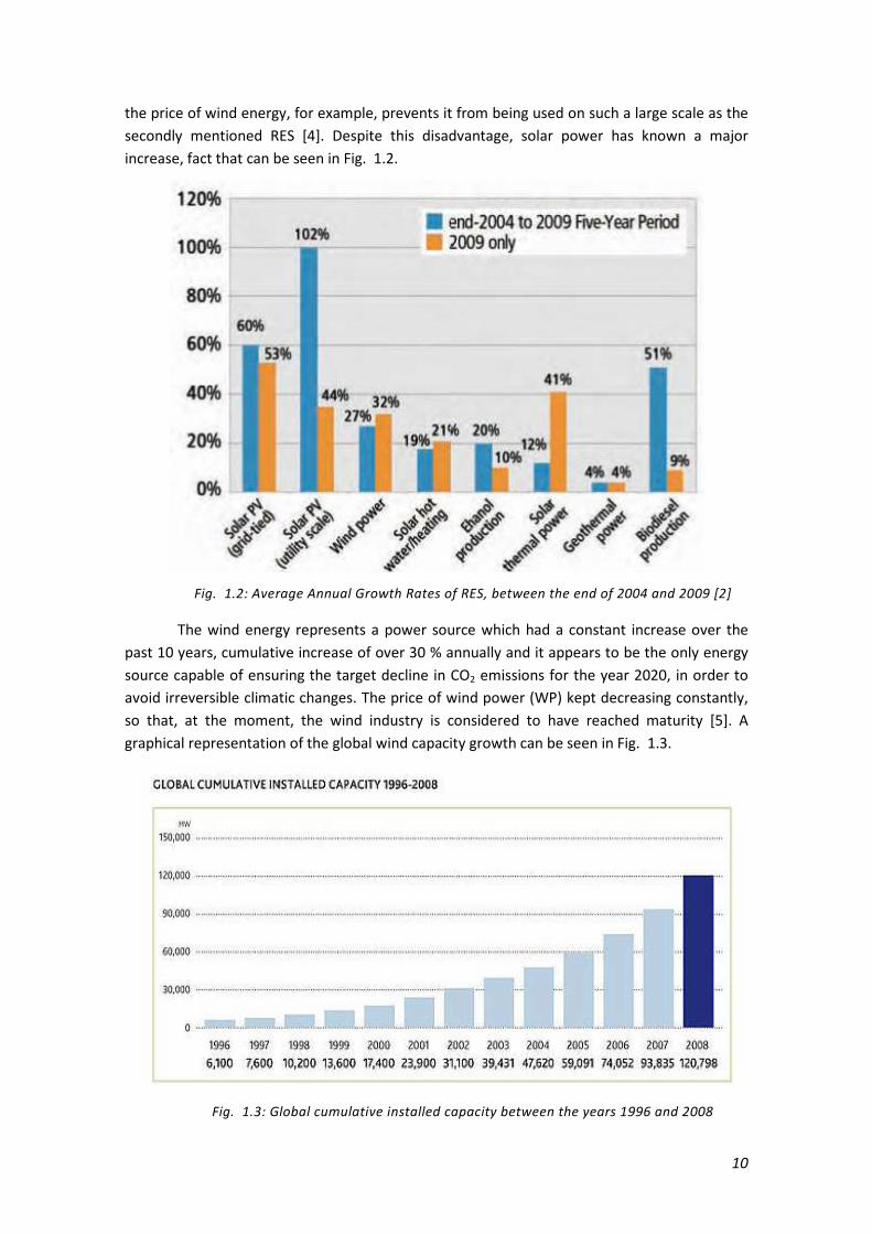
the price of wind energy, for example, prevents it from being used on such a large scale as the
secondly mentioned RES [4]. Despite this disadvantage, solar power has known a major
increase, fact that can be seen in Fig. 1.2.
Fig. 1.2: Average Annual Growth Rates of RES, between the end of 2004 and 2009 [2]
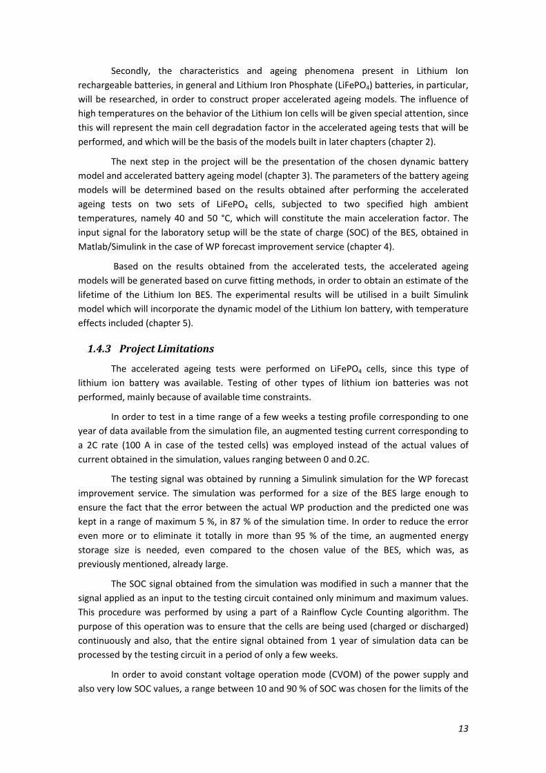
The wind energy represents a power source which had a constant increase over the
past 10 years, cumulative increase of over 30 % annually and it appears to be the only energy
source capable of ensuring the target decline in CO2 emissions for the year 2020, in order to
avoid irreversible climatic changes. The price of wind power (WP) kept decreasing constantly,
so that, at the moment, the wind industry is considered to have reached maturity [5]. A
graphical representation of the global wind capacity growth can be seen in Fig. 1.3.
Fig. 1.3: Global cumulative installed capacity between the years 1996 and 2008

11
1.2 Challenges of Wind Power Integration into the Grid
The wind is an inexhaustible energy source, available in many regions on the Globe.
This source of energy has known a major increase in popularity in the last 15 years, as a
consequence of the need for alternative nonpolluting solutions to the fossil-fuel energy
sources. The WP can be harnessed in a smaller or larger extent, by employing one single wind
turbine (WT), of various sizes, up to large wind farms, which consist of a various number of
WTs. The price of WP installations is acceptable and their environmental impact is reduced,
compared to other energy sources, such as nuclear or hydro power plants.
The major weakness of this type of energy is represented by the variability of the wind.
The WP production is strictly related to the availability of the wind, fact that makes this source
of energy much less reliable than conventional power, where the production can easily be
adjusted in every moment. Even when the wind is available, short time scale regulation is
required in case of single WT, in order to keep their power output in the desired limits. This
type of regulation is performed through pitch and yaw control. In case of large wind parks, it is
considered that wind variations below 1 minute have an insignificant effect on the farm’s
behavior, since the wind cannot affect the entire wind park instantaneously.
Long time scale WP variations caused by wild or long period wind variations cannot be
controlled through the methods applied for single WTs. This fact turns wind parks into
unreliable power generation units and other alternatives need to be provided in order to
transform them into wind power plants (WPP), capable of providing a constant power to the
consuming units, in the same manner as conventional power plants do [6].
The power output of WP units needs to be integrated into the Grid, operated by the
Transmission System Operator (TSO). The Grid functions according to a clear set of regulations
stipulated in the Grid codes, specific to each country. All the generating units involved, need to
comply with these rules. It is the reason why huge variations in the generated power, as in the
case of WP, are unacceptable, and measures have to be taken in order to avoid these
situations, else they can be the cause of severe unbalances in the Grid. As the share of WP
increases, this type of power needs to be able to cover the base load, which means to be able
to provide stable power at any point. This leads to the need of transforming the currently
employed wind farms into WPPs, with high control capabilities [7].
A stringent requirement of WP units is to be capable of delivering some services, such
as Forecast Power Improvement or Power Gradient Reduction. In the case of the firstly
mentioned service, the WP unit owners participate in the energy market where they bid with
36 hours in advance on the quantity of WP that they will be able to deliver, by keeping the
error between the bided power and the actually produced one in the allowed limits. In order
to accomplish these requirements, the power output of the WPPs must be controlled in a very
precise manner [6].
1.3 Energy Storage as a Solution
Solutions to the aforementioned issues regarding integration of WP into the Grid need
to be provided. As mentioned previously, individual control of WTs cannot be effective in case

12
of large wind parks. In order to obtain a stable power output of large WP units, Energy Storage
Systems (ESS) seem to be a viable solution. There is a multitude of available storage
technologies, suitable for various applications. In case of WP applications, where larger
quantities of power need to be stored, ESS such as pumped hydro-electric storage,
compressed air energy storage or different rechargeable battery types can be used to alleviate
the problems related to WP production. The first two technologies need specific terrain
topologies in order to be implemented, unavailable in countries which have a flat terrain, such
as Denmark. Out of the different rechargeable battery technologies, Lithium Ion battery can be
a feasible energy storage solution, due to the proper characteristics of this type of battery. The
Battery Energy Storage (BES) system can be charged whenever the WP production exceeds the
predicted power and discharged in case of underproduction, in case of the WP forecast
improvement, for example [8][9].
Probably one of the most relevant examples of BES implementation for WT
applications is represented by the 36-MW BES, built near Kermit, Texas, by Duke Energy
together with the company Xtreme Power. This storage system will serve the 153-MW Notrees
Windpower Project. The role of the BES will be to store energy whenever there is an accident
of wind and to release the stored energy whenever needed by the Grid. The total costs for the
implementation of this BES project were around 44 million $ [10].
1.4 Project Scope
1.4.1 Problem Statement
The lifetime of a BES system plays a key role the reliability of such a system integrated
into a wind power generation unit, since a good lifetime can make such a BES economically
feasible for integration into WPS. In order to assess the lifetime of the BES System in a correct
manner, research has to be carried out. It is of a capital importance to determine correctly the
influence of a service provided by a WPS on the lifetime of the ESS. Since the necessary time to
perform the tests to evaluate the lifetime of the BES is unavailable, the current project will be
focused on determining the degradation and lifetime of such a system, by using accelerated
degradation factors. The main research question that the current project will try to elucidate
can be formulated as follows:
Is it possible, and with what accuracy, to determine the degradation and lifetime of a
Lithium Ion Battery Energy Storage System under normal operation, based on accelerated
ageing models?
In order to give an appropriate answer to the research question, accelerated ageing
tests will be performed on two sets of Lithium Iron Phosphate (LiFePO4) cells, at increased
temperatures, in order to develop the accelerated ageing models that would predict the
behavior of the Li Ion BES incorporated into a WPP, under normal operating conditions.
1.4.2 Methodology
In order to develop the accelerated ageing models necessary for the BES lifetime
assessment, the project will undergo several steps. Firstly, research about the status of RES,
and about the challenges that WP brings to the Grid, will be explored (chapter 1).
13
Secondly, the characteristics and ageing phenomena present in Lithium Ion
rechargeable batteries, in general and Lithium Iron Phosphate (LiFePO4) batteries, in particular,
will be researched, in order to construct proper accelerated ageing models. The influence of
high temperatures on the behavior of the Lithium Ion cells will be given special attention, since
this will represent the main cell degradation factor in the accelerated ageing tests that will be
performed, and which will be the basis of the models built in later chapters (chapter 2).
The next step in the project will be the presentation of the chosen dynamic battery
model and accelerated battery ageing model (chapter 3). The parameters of the battery ageing
models will be determined based on the results obtained after performing the accelerated
ageing tests on two sets of LiFePO4 cells, subjected to two specified high ambient
temperatures, namely 40 and 50 °C, which will constitute the main acceleration factor. The
input signal for the laboratory setup will be the state of charge (SOC) of the BES, obtained in
Matlab/Simulink in the case of WP forecast improvement service (chapter 4).
Based on the results obtained from the accelerated tests, the accelerated ageing
models will be generated based on curve fitting methods, in order to obtain an estimate of the
lifetime of the Lithium Ion BES. The experimental results will be utilised in a built Simulink
model which will incorporate the dynamic model of the Lithium Ion battery, with temperature
effects included (chapter 5).
1.4.3 Project Limitations
The accelerated ageing tests were performed on LiFePO4 cells, since this type of
lithium ion battery was available. Testing of other types of lithium ion batteries was not
performed, mainly because of available time constraints.
In order to test in a time range of a few weeks a testing profile corresponding to one
year of data available from the simulation file, an augmented testing current corresponding to
a 2C rate (100 A in case of the tested cells) was employed instead of the actual values of
current obtained in the simulation, values ranging between 0 and 0.2C.
The testing signal was obtained by running a Simulink simulation for the WP forecast
improvement service. The simulation was performed for a size of the BES large enough to
ensure the fact that the error between the actual WP production and the predicted one was
kept in a range of maximum 5 %, in 87 % of the simulation time. In order to reduce the error
even more or to eliminate it totally in more than 95 % of the time, an augmented energy
storage size is needed, even compared to the chosen value of the BES, which was, as
previously mentioned, already large.
The SOC signal obtained from the simulation was modified in such a manner that the
signal applied as an input to the testing circuit contained only minimum and maximum values.
This procedure was performed by using a part of a Rainflow Cycle Counting algorithm. The
purpose of this operation was to ensure that the cells are being used (charged or discharged)
continuously and also, that the entire signal obtained from 1 year of simulation data can be
processed by the testing circuit in a period of only a few weeks.
In order to avoid constant voltage operation mode (CVOM) of the power supply and
also very low SOC values, a range between 10 and 90 % of SOC was chosen for the limits of the

14
input testing signal. It was decided to try to avoid as much as possible the CVOM because the
charging process is highly reduced in this region, fact that has a negative impact on the speed
of testing (number of cycles that can be tested is reduced). These testing limits were set also
because of the inaccuracies present in the components of the testing setup: power supply, DC
loads and, especially, the transducer, inaccuracies which lead to differences between the
values indicated by the software program employed and the actual values measured by a
digital oscilloscope. The errors between the two indicators lead, over time, to a translation of
the actual values of the measured indicators, which will not correspond anymore to the values
indicated by the testing program. The accumulation of the errors determined major
differences between the values indicated by the program and the actually measured values,
turning off the setup because of stopping conditions fulfillment, even though the program
showed different values. An attempt to resolve the problems caused by the inaccuracies of the
setup devices was implemented by estimating a correction coefficient for the scaling equation
of the current calculation.
Even though the minimum allowed limit for the voltage of this category of lithium ion
cells is 2 volts, in the program the minimum voltage condition to disconnect the setup was set
to 2.33 volts because of the voltage limitation of the DC loads, which need a well defined
minimum voltage in order to be able to discharge with a certain current. In case of the
employed setup, which uses two cells connected in series, a minimum voltage of 4 volts was
insufficient in order for the electronic loads to discharge the cells with a 2C rate.
The allocated time for testing at each of the two temperatures was brief, because of
the available time restrictions which impose the following limitations: the generated
accelerated ageing, based on the tests, may not have a satisfactory level of accuracy because
of the insufficient degradation of the tested cells. Besides, the small number of ageing points
measured experimentally leads to an unclear tendency of the ageing factors, making the
estimation of the curve and surface fitting equations more difficult, which at the same time,
worsens the precision of the ageing model and lifetime prediction of the BES.
The calendar life ageing effect at different temperatures could not be measured; the
capacity fade due to this effect is calculated from the manufacturer data and the impedance
increment is neglected, as no concrete data was found in the literature.
The ageing tests were performed at only two high ambient temperature levels. The
climatic chamber controls the temperature through three thermocouples located on the sides
of the inner box. Thus, the temperature control was not performed on the surface of the cells,
but in the ambient environment of the climatic chamber, as these thermocouples could not be
moved and placed to a different place.
The daily available testing time was of 6 hours and a continuous testing for the whole
year signal could not be performed. As a consequence, the climatic chamber had to be heated
up every morning with the cells inside before start of the testing procedure, which makes the
separation of cycling and calendar ageing effects more difficult to accomplish. Thus, this
separation of the ageing effects was not taken into consideration in the present work.

15
2 Lithium Ion Battery Characterization
The chapter will focus on performing a characterization of the main aspects regarding
the lithium ion battery technology, starting with the main characteristics of the more general
lithium battery category, followed by a description of the lithium battery technologies, with
emphasis on the Lithium Iron Phosphate battery properties and lithium ion battery technology
ageing phenomena. The chapter will be concluded by a short justification of the chosen battery
technology type.
2.1 Lithium Battery Properties
Lithium batteries are a category of rechargeable batteries with high energy and power
capabilities, due to the high reactivity of Lithium. These good capabilities of this type of battery
make it suitable for high power applications. The anode of lithium batteries is usually made of
Carbon, while the cathode is composed of Lithium Cobalt dioxide or a Lithium Manganese
compound. The electrolyte is represented by a lithium salt in an organic solvent.
This type of rechargeable battery presents the following advantages:
• High cell voltage compared to other rechargeable battery technologies located
around 3.6 volts, which means higher energy and power capabilities
• High energy and power densities, as mentioned before
• No memory effect, a major advantage compared to other battery technologies
• Low weight, compared to other battery types
• Lithium cell are available in very small sizes, making them suitable for low power
applications
• They are available in a wide range of capacities, varying between less than 500
mAh to more than 1000 Ah
• They have a long cycle life, ranging between 1000 and 3000 cycles
• Can be discharged at a rate of 40C or more and a fast charging is possible
• Lithium batteries have a very low self discharge rate, of about 5-10 % per month
• Very high coulombic efficiency (capacity discharged over capacity charged) of
almost 100 %
The most important shortcomings of this battery technology can be synthesized as
follows:
• Special safety precautions need to be taken in order to ensure that the operating
conditions of the lithium battery are kept in between the safety limits, because of
the high reactivity of this type of battery. These special precautions have to be
taken also in the case of shipment of this battery type

16
• Overcharging lithium batteries leads to their overheating and capacity loss, while
discharging them below the limit of 2 volts can cause them serious damage
• Their internal impedance is higher than that of equivalent NiCd batteries
• Measuring the SOC of lithium cells is more complex than in the case of other
rechargeable battery technologies, because of the flatness of discharge voltage-
SOC curve of this battery
• The price of lithium batteries is still high compared to other Lead Acid batteries in
the case of high power applications, but as their use is increasing in this type of
applications, their price is expected to decrease.
• The cost of power of lithium rechargeable batteries is estimated to be around
1600 €/kW, while the energy costs are evaluated to be around 320 €/kWh.
2.2 Lithium Battery Technologies
The Lithium batteries can be divided into several categories, which are being treated in
the following paragraphs:
Lithium Ion batteries have the major advantage, compared to the more general
lithium battery category, that the problem regarding the high reactivity of lithium has been
eliminated. The anode of Lithium Ion battery is composed of Lithium dissolved as ions, while
the cathode can be one of the following oxides: Lithium Cobalt Oxide (LiCoO2), Lithium
Manganese Oxide (LiMn2O4) and Lithium Nickel Oxide (LiNiO2). The electrolyte is formed of
Lithium salt.
In case of this battery technology, the Lithium metal has to be eliminated during all the
periods of charging or discharging of the cells. The Lithium ions are in the positive electrode
when the cell is discharged and in the positive electrode when the cell is charged and they are
moving from one electrode to the other through the electrolyte. The voltage of the cell is given
by the difference in the in energy between the Li+ ions that are present in the crystalline
structure of the two electrodes. Because of the high flexibility in the construction of lithium ion
cells and their chemistry, the electrodes can be built with very high surface areas, enabling
them for high power applications. Lithium-ion cells have no memory effect, long cycle life and
good discharging capabilities [11][12].
Lithium polymer batteries have as major difference compared to other types of
batteries, the fact that they utilise a different type of electrolyte, namely a dry polymer
electrolyte which does not conduct electricity, but allows exchange of ions. One of the
advantages of this type of batteries is the lack of heavy protective cases, needed in the case of
other types of cell, cases unnecessary in case the electrolyte in not liquid. This property makes
lithium polymer cells less sensitive to overcharge or damage. They are also called Solid State
cells. Solid electrolyte cells have a long life but a low discharge rate. They have a low
conductivity, because of the high internal resistance, which is their main flaw. The conductivity
of the cell can be increased by heating the cell to 60 °C, but this makes it unsuitable for high
power applications.

17
Some of the advantages of Lithium-ion polymer batteries are very low profile, flexible
form factor, lightweight and improved safety. The drawbacks of Li-ion polymer batteries are
mainly the next ones: lower energy density and decreased cycle life compared to Li-ion
batteries, high manufacturing costs, no standard sizes and a higher cost/kWh than for Li-ion
cells.
Lithium Cobalt is a mature battery technology, characterized by a long cycle life and
high energy densities. The polymer electrolyte makes this type of cell safer than the other
technology types that employ fluid electrolytes where electrolyte leakages are possible, in case
of mistreatment. The cell nominal voltage is of 3.7 volts and this type of battery is being
produced by a wide range of manufacturers. One of the main drawbacks of LiCoO2 batteries is
the relatively low discharge current, translated into charge and discharge rates limited to 1C.
Another major weakness of this battery type is the increase in internal resistance that occurs
with ageing and cycling [11][12].
Lithium Manganese (LiMn2O4) batteries: Lithium Manganese oxide cells have a higher
nominal voltage than Lithium Cobalt cells, voltage rated at 3.8 to 4 volts, but their energy
density is 20 % less. The Manganese oxide forms a three dimensional spinel that improves the
ion flow between the electrodes, resulting in lower internal resistance than for LiCoO2
batteries and in an incremented loading capacity. A low internal resistance means higher
charge and discharge currents. LiMn2O4 batteries bring improvements to the Lithium Ion
batteries, such as lower costs and higher temperature capabilities. This technology is more
stable than LiCoO2 batteries, which makes it a safer technology. The major drawback of
LiMn2O4 batteries is represented by their low capacity compared to Cobalt based batteries,
which is with about 50 % less [11][12].
Lithium Nickel (LiNiO2) batteries: these cells are able to provide up to 30 % bigger
energy density compared to Cobalt based Lithium cells. The voltage of the cell is of 3.6 volts
and this type of cell has the highest exothermic reaction, which could produce cooling
problems in high power applications. Therefore, this battery technology is not being employed
in too many applications [12].
Lithium Nickel Cobalt Manganese (Li(NiCoMn)O2 (NCM)) batteries: the cathode of this
type of batteries is formed of cobalt, nickel and manganese. These form a multi-metal oxide in
the crystal structure to which lithium is added. The cell maximum voltage of this battery
technology is of 4.1 volts. If the NCM cell would be charged to 4.2 volts, which is the charging
voltage of Cobalt and Manganese based cells, the cycle life of the cell would be reduced from
the usual value of 800 cycles to about 300 cycles [11][12].
Lithium Titanate (LiTiO3) batteries: Lithium Titanate is a modified Li Ion battery that
uses lithium titanate nanocrystals on the surface of the anode, instead of carbon. The main
advantages of this battery technology compared to the other battery systems are the
following:
• A higher temperature range, which can vary from -40 °C to 55 °C and can go up to
65 °C
• An increase in the power level, that can be up to three times bigger than in
conventional batteries

18
• A longer cycle life, than can exceed 12 000 cycles
• Faster charge/discharge rates (10 minutes) than in the case of other batteries
• Higher tolerance to operational abuses
The main drawback of this technology is represented by the lower cell voltage, which
leads to lower power and energy densities [13] [14].
Lithium Iron Phosphate (LiFePO4) Batteries: Lithium iron phosphate represents a
viable option for the cathode material for the Lithium Ion batteries because of its low cost,
environmental friendliness, long cycle and calendar lives (chemical stability) and good capacity
(170 mAh/g). LiFePO4 batteries are incombustible in case of misuse during charging or
discharging, they are more stable during overcharge or short circuit conditions and they can
withstand high temperatures without decomposing. By doping the cell with transition metals
the nature of the active materials can be changed, leading to reduced internal impedance. The
operating performance of the cell can be improved by changing the identity of the transition
metal. This way, the voltage and the specific capacity of the active materials can be brought to
the desired level [12].
The charging voltage of this type of cell should not exceed the value of 3.6 volts and
the minimum discharge voltage should not go lower than 2 volts, in order to maintain a good
life time for the cell.
The main characteristics of LiFePO4 batteries are presented in the following:
• Nominal operating voltage of 3.3 V
• No memory effect
• Energy efficiency of 95 %
• Charge time less than 2 hours
• Self discharge of 8 % per month [15]
• Specific energy of 150 Wh/kg
• Energy density of 400 Wh/l [16]
The main advantages of this type of Lithium battery are synthesized in the following:
• Safe technology, which means that in case of overcharge it will not explode or
catch fire
• It has a constant discharge voltage on a big portion of a discharging cycle, which
implies the use of maximum power until nearly full discharge
• It has a 2000 cycles life, compared to 300 for lead acid batteries
• This type of battery has a high discharge rate capability: 35C continuously
• It can be left for longer periods of time partially discharged, without causing
permanent degradation, unlike lead acid batteries
• Small self discharge rate, compared to lead acid batteries
19
• Can be used safely in ambient temperature up to 60 °C, without significant
degradation in performance
• Does not contain any toxic metals, such as lead, cadmium nor corrosive acids or
alkaline, fact that makes LiFeO4 the most environmentally friendly battery
technology
• These cells are solid, which makes them less vulnerable to failures over time
caused by vibrations
• It has the highest power density of all the commercially available lithium batteries
The main drawbacks of this material are its low electronic conductivity and the small
Li-ion diffusivity, which limit its application [17] [18] [11][19].
2.3 Lithium Ion Battery Ageing Mechanisms
The ageing of a battery represents the modification of its properties as a consequence
of time and use. The main properties are the available energy and power of the cell and
properties related to the cell integrity, such as leakage, cell dimensions. The energy loss is
mainly the result of the reactions between the active materials in the cell, which means a
reduction of the cell capacity, and from an increase of the internal impedance of the cell,
which results in a lowered available cell voltage. The power fade of the cell is directly related
to the increase in the internal impedance of the cell.
The ageing mechanisms can be divided into two categories: ageing because of cell
cycling (charging/discharging of the cell) and ageing on storage (when the cell is on rest). The
cycling has a negative impact on the reversibility of the materials, while the interactions
between the electrode materials and electrolyte are mainly responsible for ageing on storage
and are strongly influenced by time and temperature. The ageing on storage is an effect of the
side reactions that occur between the active materials of the Lithium Ion cell, while the cycling
adds other effects, such as volume variations or concentration gradients. Although the two
ageing mechanisms are considered to act independently on the cell and their effects are being
added, there are also many interactions between them, interactions that contribute to an
accelerated degradation of the cell’s properties [20].
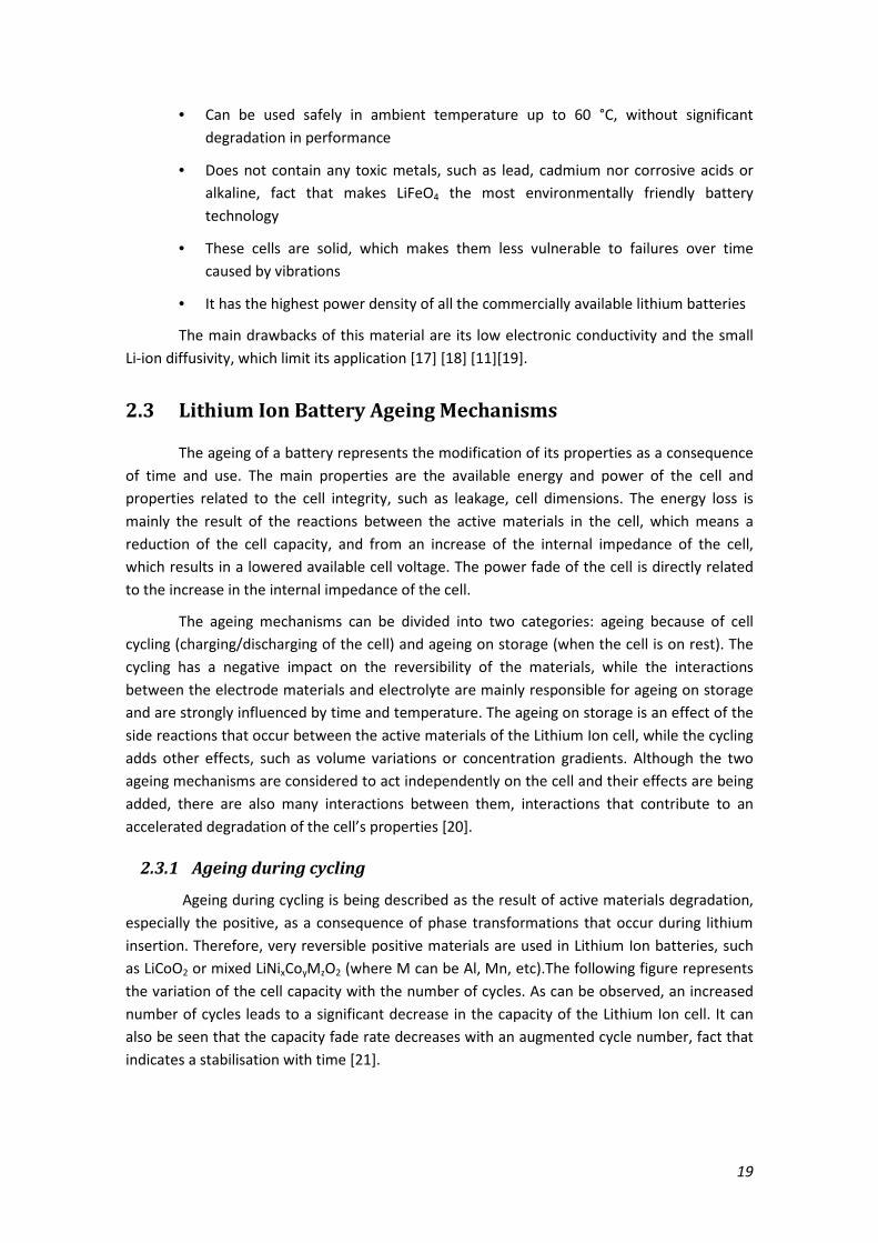
2.3.1 Ageing during cycling
Ageing during cycling is being described as the result of active materials degradation,
especially the positive, as a consequence of phase transformations that occur during lithium
insertion. Therefore, very reversible positive materials are used in Lithium Ion batteries, such
as LiCoO2 or mixed LiNixCoyMzO2 (where M can be Al, Mn, etc).The following figure represents
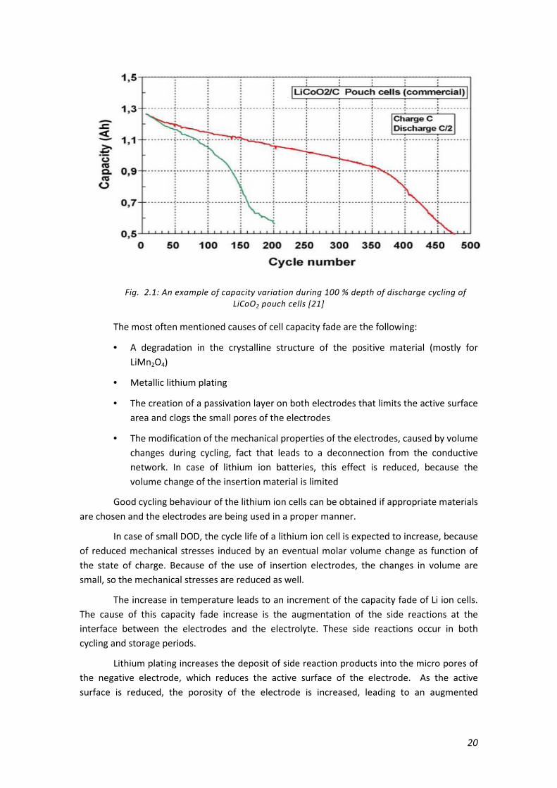
the variation of the cell capacity with the number of cycles. As can be observed, an increased
number of cycles leads to a significant decrease in the capacity of the Lithium Ion cell. It can
also be seen that the capacity fade rate decreases with an augmented cycle number, fact that
indicates a stabilisation with time [21].
20
Fig. 2.1: An example of capacity variation during 100 % depth of discharge cycling of LiCoO2 pouch cells [21]
The most often mentioned causes of cell capacity fade are the following:
• A degradation in the crystalline structure of the positive material (mostly for
LiMn2O4)
• Metallic lithium plating
• The creation of a passivation layer on both electrodes that limits the active surface
area and clogs the small pores of the electrodes
• The modification of the mechanical properties of the electrodes, caused by volume
changes during cycling, fact that leads to a deconnection from the conductive
network. In case of lithium ion batteries, this effect is reduced, because the
volume change of the insertion material is limited
Good cycling behaviour of the lithium ion cells can be obtained if appropriate materials
are chosen and the electrodes are being used in a proper manner.
In case of small DOD, the cycle life of a lithium ion cell is expected to increase, because
of reduced mechanical stresses induced by an eventual molar volume change as function of
the state of charge. Because of the use of insertion electrodes, the changes in volume are
small, so the mechanical stresses are reduced as well.
The increase in temperature leads to an increment of the capacity fade of Li ion cells.
The cause of this capacity fade increase is the augmentation of the side reactions at the
interface between the electrodes and the electrolyte. These side reactions occur in both
cycling and storage periods.
Lithium plating increases the deposit of side reaction products into the micro pores of
the negative electrode, which reduces the active surface of the electrode. As the active
surface is reduced, the porosity of the electrode is increased, leading to an augmented
21
capacity fade on cycling. A temperature decrease is accelerating the fade rate, since the limit
at which lithium plating occurs is diminished.
In case a change in the volume of the carbon based material occurs during cycling,
there will be a degradation of the Solid Electrolyte Interface (SEI), followed by a restoration of
this layer. This phenomenon takes place at the cost of lithium consumption and results in a
severe capacity fade of the lithium ion cell.
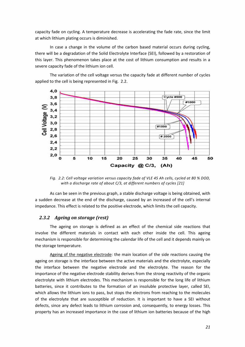
The variation of the cell voltage versus the capacity fade at different number of cycles
applied to the cell is being represented in Fig. 2.2.
Fig. 2.2: Cell voltage variation versus capacity fade of VLE 45 Ah cells, cycled at 80 % DOD, with a discharge rate of about C/3, at different numbers of cycles [21]
As can be seen in the previous graph, a stable discharge voltage is being obtained, with
a sudden decrease at the end of the discharge, caused by an increased of the cell’s internal
impedance. This effect is related to the positive electrode, which limits the cell capacity.
2.3.2 Ageing on storage (rest)
The ageing on storage is defined as an effect of the chemical side reactions that
involve the different materials in contact with each other inside the cell. This ageing
mechanism is responsible for determining the calendar life of the cell and it depends mainly on
the storage temperature.
Ageing of the negative electrode: the main location of the side reactions causing the
ageing on storage is the interface between the active materials and the electrolyte, especially
the interface between the negative electrode and the electrolyte. The reason for the
importance of the negative electrode stability derives from the strong reactivity of the organic
electrolyte with lithium electrodes. This mechanism is responsible for the long life of lithium
batteries, since it contributes to the formation of an insoluble protective layer, called SEI,
which allows the lithium ions to pass, but stops the electrons from reaching to the molecules
of the electrolyte that are susceptible of reduction. It is important to have a SEI without
defects, since any defect leads to lithium corrosion and, consequently, to energy losses. This
property has an increased importance in the case of lithium ion batteries because of the high
22
surface area of the negative electrode, and it can be a source of ageing. On the other hand, in
case the SEI is too thick, it can take to an increase in the internal impedance of the lithium ion
cell, which means augmented capacity and power fades. This is why only a few organic
materials are appropriate to be used as solvents for the electrolyte [21][20] [22].
The SEI is also formed at the carbon surface and the lithium lost in this case is of at
least 10 % of the inserted capacity, because of the higher surface area. However, because of
the fact that the SEI is formed only once, at the first charge and remains stable during cycling,
the stability of lithium ion batteries is ensured. This stability is also given by the fact that there
is only a very small molar volume change of the carbon material during charging and
discharging.
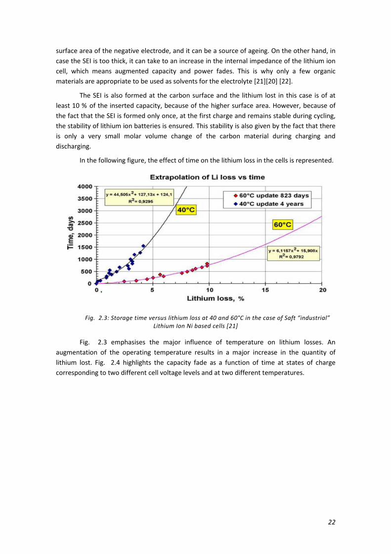
In the following figure, the effect of time on the lithium loss in the cells is represented.
Fig. 2.3: Storage time versus lithium loss at 40 and 60°C in the case of Saft “industrial” Lithium Ion Ni based cells [21]
Fig. 2.3 emphasises the major influence of temperature on lithium losses. An
augmentation of the operating temperature results in a major increase in the quantity of
lithium lost. Fig. 2.4 highlights the capacity fade as a function of time at states of charge
corresponding to two different cell voltage levels and at two different temperatures.

23
Fig. 2.4: Capacity versus time for Li ion Ni based cells, at 3.8 and 3.9 volts voltage level, at 40 and 60°C [21]
From the above figure, it can be concluded that the temperature is one of the major
factors that lead to an increase of the capacity fade. It can also be seen that as long as the
temperature is not extremely high, the voltage (and also the SOC) does not have a major
influence on the capacity variation of the lithium ion cell, since the electrode reactivity, which
is related to the electrode voltage, has only a reduced dependence upon the state of charge of
the negative electrode. The same conclusions can be drawn in the case of internal resistance
increase with time in Fig. 2.5, where rest and float voltages were applied to two sets of cells.
As in the case of the capacity, the impedance variation reduces with time, stabilizing,
eventually, around a steady-state value.
Fig. 2.5: Example of internal resistance variation during storage at 30 °C, for several float
or rest voltages [21]
24
In case of high temperatures and high SOCs, a significant influence of the cell voltage
on the capacity fade and internal impedance increase can be observed because of the positive
electrode.
Ageing of the positive electrode: as temperature increases, the oxidation of the
positive electrode against the electrolyte starts to be the major ageing event. Since this
oxidation phenomenon is directly influenced by the interface voltage, it depends on the SOC of
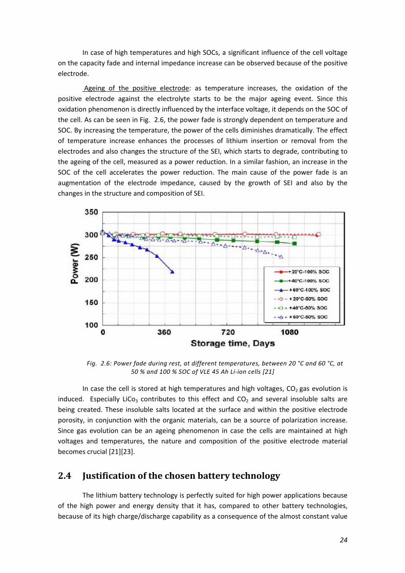
the cell. As can be seen in Fig. 2.6, the power fade is strongly dependent on temperature and
SOC. By increasing the temperature, the power of the cells diminishes dramatically. The effect
of temperature increase enhances the processes of lithium insertion or removal from the
electrodes and also changes the structure of the SEI, which starts to degrade, contributing to
the ageing of the cell, measured as a power reduction. In a similar fashion, an increase in the
SOC of the cell accelerates the power reduction. The main cause of the power fade is an
augmentation of the electrode impedance, caused by the growth of SEI and also by the
changes in the structure and composition of SEI.
Fig. 2.6: Power fade during rest, at different temperatures, between 20 °C and 60 °C, at 50 % and 100 % SOC of VLE 45 Ah Li-ion cells [21]
In case the cell is stored at high temperatures and high voltages, CO2 gas evolution is
induced. Especially LiCo3 contributes to this effect and CO2 and several insoluble salts are
being created. These insoluble salts located at the surface and within the positive electrode
porosity, in conjunction with the organic materials, can be a source of polarization increase.
Since gas evolution can be an ageing phenomenon in case the cells are maintained at high
voltages and temperatures, the nature and composition of the positive electrode material
becomes crucial [21][23].
2.4 Justification of the chosen battery technology
The lithium battery technology is perfectly suited for high power applications because
of the high power and energy density that it has, compared to other battery technologies,
because of its high charge/discharge capability as a consequence of the almost constant value

25
of the voltage on a major part of its voltage characteristic, meaning a constant, close to
maximum, power delivery on the area. Also, the required size for this technology is much
lower than for other battery types with the same electrical capabilities. The major flaw of this
battery technology consists in the high reactivity of lithium, which implies a careful handling of
this type of battery.
The disadvantage of the lithium battery technology can be successfully countered by
the LiFePO4 battery, which is characterised by good thermal and chemical stability, meaning
increased safety, making them appropriate for high power applications, such as Battery Energy
Storage Systems. The increase in safety is related to the utilisation of transition metals in the
cathode. Some of the main strengths of this type of battery are its high power density, big
cycle life and no memory effect [18][11].

26

27
3 Battery Lifetime Modelling
The present chapter will delve into the modelling of batteries, putting the accent on
modelling of the degradation processes present in the batteries. Firstly, some relevant battery
models will undergo a brief description, followed by a description of the simulation file utilised,
and a depiction of the employed battery equivalent model, with emphasis on the degradation
parameters, will conclude the chapter.
3.1 Battery lifetime models
A correct assessment of the lifetime of batteries is becoming vital, as their use in
various applications is facing a continuous augmentation. The economic implications of a
correct battery lifetime estimation can be major, leading to an improved quality of the services
in which this type of storage elements are involved, for reasonable prices.
Three main aspects are considered regarding battery modelling. The first category of
battery models, named performance or charge models, focuses on modelling the state of
charge of the battery.
The second type of model, the voltage model, is centred around the modelling the
battery voltage, which means a more in depth emphasis on the battery losses. The third type
of model, the lifetime model, assesses the influence of a certain model scheme on the battery
lifetime.
These three categories of battery models can be independent or they can be
integrated into a more complex battery model, in an attempt to represent all the aspects
regarding battery behaviour. The advantage of complex models resides in their ability to model
the degradation in the battery performance as the battery is operated.
The lifetime models can be classified into two categories:
• Post-processing models
• Performance degradation models
The Post-Processing models do not contain information about the battery
performance degradation processes and are utilised to analyse measurement data from real
systems.
The main methods used for calculating the lifetime degradation of the batteries are
the Ah-throughput counting method and the Cycle counting method.
The Ah throughput counting method consists of simply counting the charge that flows
through the battery in a certain amount of time. The basic procedure takes into consideration
only the charge through the battery, but weighting factors can be taken into account, factors
dependent on the value of the charge or discharge current through the battery and on the SOC
of the system. The end of life criterion is based on datasheet values for the Ah throughput,
provided by the battery manufacturer.

28
The Cycle counting method is insisting, mainly, on two aspects of the battery: the
current and state of charge of the battery. In this method the major factor acting on the
lifetime degradation of the battery is considered to be given by the depth of discharge of the
battery cycles. Some weighting factors can be included in this method which can take into
account the SOC at which the cycles occur. The end of lifetime condition is represented by the
equivalent number of cycles for a certain depth of discharge guaranteed by the manufacturer.
The Performance degradation models are a combination of a performance model and
a lifetime model, and they involve an online calculation and update of the degradation of the
battery parameters.
In real life batteries, the end of life is defined as the loss in their ability to provide the
nominal capacity and nominal power, losses known as capacity and power fade, respectively.
The end of life criterion in case of the battery capacity is generally considered to be 80 % of the
nominal capacity. This type of modelling considers all the aforementioned models, meaning
that the variations in the battery voltage, battery capacity and impedance are calculated
permanently during battery degradation process [24].
There are two main methods employed in order to evaluate the battery performance:
the first method uses an equivalent circuit model, while the second method tries to model the
changes in the physical characteristics of the battery components (electrodes, electrolyte)
during the battery ageing process.
In the first method utilised, the values of the voltage of the equivalent circuit and
battery capacity are updated permanently during the operation of the battery. The second
method which employs the physical properties model puts emphasis on the changes occurring
in the structure of the electrodes leading to modified diffusion processes electrolyte and,
eventually, changes in the battery voltage and capacity.
The first type of circuit model requires data that can be provided by the manufacturer,
while the physical properties model involves access to details regarding the manufacturing
process of the cell, details that are, generally, not available.
The next section is dedicated to a brief description of some representative battery
models present in the literature. The models will try to point out the theoretical aspects
discussed in the last section. They were employed in case of a lead-acid battery.
Ah Throughput Models
The assumption in this type of model is that the amount of energy that can go through
a battery before it requires replacement is fixed and independent of depth of discharge of the
cycles or other parameters. The energy throughput is calculated based on the depth of
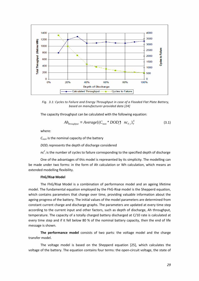
discharge versus number of cycles to failure graph, provided by the manufacturer (Fig. 3.1).
This calculation is based on the assumption that for most of the batteries, by multiplying the
number of cycles to end of life corresponding to a specified DOD by the energy processed
during that cycle.
29
Fig. 3.1: Cycles to Failure and Energy Throughput in case of a Flooded Flat Plate Battery, based on manufacturer-provided data [24]
The capacity throughput can be calculated with the following equation:
,( ) Xthroughput nom i F i YAh Average C DOD nc= ∗ ∗ (3.1)
where:
Cnom is the nominal capacity of the battery
DODi represents the depth of discharge considered
ncFi is the number of cycles to failure corresponding to the specified depth of discharge
One of the advantages of this model is represented by its simplicity. The modelling can
be made under two forms: in the form of Ah calculation or Wh calculation, which means an
extended modelling flexibility.
FhG/Risø Model
The FhG/Risø Model is a combination of performance model and an ageing lifetime
model. The fundamental equation employed by the FhG-Risø model is the Shepperd equation,
which contains parameters that change over time, providing valuable information about the
ageing progress of the battery. The initial values of the model parameters are determined from
constant current charge and discharge graphs. The parameters are updated at every time step
according to the current input and other factors, such as depth of discharge, Ah throughput,
temperature. The capacity of a totally charged battery discharged at C/10 rate is calculated at
every time step and if it fell below 80 % of the nominal battery capacity, then the end of life
message is shown.
The performance model consists of two parts: the voltage model and the charge
transfer model.
The voltage model is based on the Shepperd equation [25], which calculates the
voltage of the battery. The equation contains four terms: the open-circuit voltage, the state of

30
charge of the battery, the ohmic losses in the battery by using the internal resistance and the
charge factor over voltage, which has a major effect when the battery is nearly charged or
discharged.
The charge transfer model is utilized in order to compute the SOC of the battery. The
SOC is obtained by integrating the current over time, but some of the charge is lost due to
gassing processes, meaning that not all the charge is contained in the chemical processes
occurring inside the battery. The gassing phenomenon is dependent on the battery voltage.
The higher the value of the voltage, the more gassing occurs, leading to a decrement of the
current flowing through then battery.
The ageing model contains the equations corresponding to two ageing mechanisms:
corrosion and active material degradation.
The corrosion process is considered as the oxidation of the Pb contained in the positive
electrode into PbO and PbO2. The oxidation causes a lower conductivity and lower density of
the oxidized material. The lower conductivity means an increase of the resistive losses and the
density modification leads to mechanical stresses in the plate grid, implying, eventually, a loss
of contact between the active material and the grid.
The active material degradation is a consequence of the reordering of the structure of
the active material, as a consequence of battery cycling. With each new applied cycle, the
active material becomes more crystalline, meaning a reduction of the electrode pores through
which the electrolyte flows and also the surface area available for ion transport. So,
degradation means both a loss in the efficiency of the active material and a loss of the material
itself, phenomena which lead to a capacity fade of the battery [24].
The UMass Model (Kinetic Battery Model)
The UMass Model incorporates all the three battery models: a voltage model, a
capacity model and a lifetime model. The model uses parameters based on data of the physical
processes of the battery, data that was determined experimentally. The capacity model was
built based on the assumption of a first order chemical rate process. The voltage model is a
mix of an adaptation of the Battery Energy Storage Test model and capacity estimates
obtained from the capacity part of the model. The lifetime model was initially based on the
number of cycles until the end of life of the battery, as a function of the depth of discharge.
This initial condition was modified in order to be able to predict the battery lifetime in case of
random cycles, by employing a rainflow cycle counting algorithm.
The voltage and capacity parts of the model are based on fact that the battery is
considered as being a current source in series with an internal resistance, R0. The voltage of
the current source is E and the voltage at the battery terminals is V. This representation can be
visualized in Fig. 3.2.

31
Fig. 3.2: Battery Model Equivalent Circuit [24]
Model for the Battery Lifetime Verification
This model is intended for lifetime estimation and validation of lithium ion batteries,
mainly employed in automotive applications. In order to fulfil this purpose a series of stress
factors are applied to a life test matrix consisting of several lithium ion batteries. The applied
stress factors are: temperature, state of charge, rate of discharge energy throughput, and
discharge and regenerative pulse power levels.
The design of the life test matrix is made based on well defined experiment principles.
The testing procedure starts with the selection of an initial matrix of stress conditions.
An acceleration factor is estimated for each test condition. The total number of cells
employed for testing plays a fundamental role in the planning. The life test experiment
includes a core matrix and a supplemental matrix. In the core matrix, a certain number of cells
are tested in on rest under different stressing factors, in order to establish their calendar life,
and the same number of cells is tested by cycling them in order to determine their cycle life.
The supplemental life test matrix includes cell operation under special conditions, such as cold
cranking or operation of the cells at low temperatures, in order to observe the effects of these
conditions on the lifetime of the cells.
During testing, the indicator of the cell performance is the area-specific impedance
(ASI) of the cell, whose increase is the main responsible factor for the power fade mechanism.
The increase of the ASI is strongly depending on the calendar life and cycle life acceleration
factors, who are, themselves, dependent on temperature.
In case of the core life test matrix, the expected lives on test are obtained by dividing
the calendar life by the acceleration factors. The calendar life is dependent on the power fade
and rate of change of ASI. The parameters β0, β1 and ASI0 which form the model are dependent
on the variation of ASI, power fade, while the parameter ASI0 is considered to be the ASI of the
cells at their beginning of life. Subsequently, the ASI at a specified moment in time is calculated
with these three parameters. From these parameters the expected accelerated factor and
excepted life on test is calculated for each cell of the core matrix.
The next step is the determination of the estimated lives on test, since there can be
significant variation from the expected values of the parameters, variations caused by cell-to-
cell differences and by ASI measurement errors. These parameter variations can lead to
considerable differences between the expected lives of test and the estimated ones from the
32
measurements. The estimated parameters ^ ^
0 1,β β and ^
0ASI are calculated and, subsequently,
the estimated life on test ^
TestL is obtained from them.
The standard deviation of the life on test for each testing condition is dependent on
the number of cells tested at that specified condition. The standard deviations of the lives on
test are employed together with the acceleration factor corresponding to the test conditions in
order to obtain the standard deviation of the estimated calendar life [26].
3.2 Description of the Simulink Model
During the first chapter the necessity for incorporating ESS into various WP generating
units was motivated. It was proved that a future increase of the WP share in the Electrical Grid
could be the source of major problems for the Grid, because of the wild fluctuations and
unpredictable behaviour of the wind. The ESS can be a viable solution for mitigating these
problems and, on the other hand, for turning Wind Farms into generating units capable of
covering a required percentage of the base load in the Grid.
In order to assess the impact of a BES System on the capabilities of a WP based
generation unit of providing a certain service, a Simulink model will be constructed.
The Forecast Improvement Service was chosen to be the service under which the
interaction between the WP unit and the BES will be studied and the improvements that the
incorporation of the BES into the WPP will bring, from the power flow point of view.
The Simulink model will contain as input data a wind power data, corresponding to,
either, a single 2-MW WT, or to a wind park containing 50 WTs, with the nominal power of 2
MW for each turbine. The second input into the simulation file is represented by a WP forecast
data obtained from the WP data undergoing an error addition or subtraction, depending on
whether there is an overestimation or underestimation of the forecasted power. The error is
added or subtracted from the mean value of the WP, mean taken on a short period of time (15
minutes). This error contains two components: the systematic error which increases over the
time, but after each 36 hours period is reverted to zero, since a new WP forecast is made every
36 hours. There are several WP forecast prediction methods, but a complex statistical method
was implemented for the present forecast generation, a forecast method in which the
systematic error at the end of the 36 hours of prediction does not exceed the value of 10 % of
the nominal power of the WP generating unit. The other component of the forecast error is
corresponds to the random error, which accounts for around 5 % of the nominal power of the
WPS [27][28].
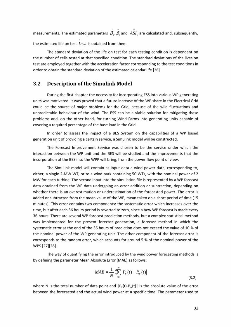
The way of quantifying the error introduced by the wind power forecasting methods is
by defining the parameter Mean Absolute Error (MAE) as follows:
1
1( ) ( )
N
F Wt
MAE P t P tN =
= ⋅ −∑ (3.2)
where N is the total number of data point and |PF(t)-Pw(t)| is the absolute value of the error
between the forecasted and the actual wind power at a specific time. The parameter used to

33
estimate the precision of a forecast prediction method is the Normalised Mean Absolute Error
(NMAE), defined as the value of the MAE divided by the nominal power of the WPS. It can be
concluded that both types of error are dependent on the size of the studied WPS [29][28].
The WP and forecast signal are the inputs of the “Forecast Improvement” service block
in the model, service that fulfils the gradient condition stipulated in the German Grid codes,
gradient condition which allows a maximum variation of the wind power of 10 % per minute of
the nominal power of the considered wind power system’s nominal power.
The BES has to be able to produce an improvement of the wind power input such that
the NMAE between output power of the WPS with the BES system included and the forecasted
WP would be reduced to at least 5 % in 95 % of the considered time.
The simulation file contains an initialisation block in which some of the input
parameters of the simulation are set. The parameters introduced in this block are the
maximum allowed gradient variation per minute, the nominal power of the studied WPS, the
size of the BES, given as fraction of the nominal power of the WPS in the case of the storage
power, PS, and as number of hours in which the BES is able to provide this storage power, in
the case of the storage energy, Es. The last parameter defined in this initialisation block is the
temperature at which the system will operate. The outputs of this block are number of cell
that will form the BES, influenced mainly, by the storage power, Ps and the maximum allowed
current that will act on the BES during the charging/discharging process.
In the “Forecast Improvement” block the Mission profile signal is generated, which is,
basically, the difference between the forecast power data and the WP data inputs, and
represents the power that the BES should be able to provide ideally.
The obtained Mission Profile power signal is the input of the next block in the
simulation, the “Battery Energy System” block, block composed of two subsystems: the
“Converter” and the “Battery Model” subsystems, respectively. The input of the “Converter”
block is the Mission Profile power. In case the Mission Profile exceeds the 5 percent set limit of
the nominal power of the WPS, the difference between the Mission Profile and this allowed
fraction of the nominal power is divided by the BES’s voltage and the BES is charged or
discharged with the current corresponding to this division. So, basically, the BES is charged or
discharged only with the power quantities corresponding to an error larger than 5 % between
the forecast and actual wind powers. The obtained current from the Mission Profile is utilised
as an input to the “Battery Model” subsystem, in which the BES voltage is obtained, as a
product of the individual cell’s voltage, multiplied by the number of cells composing the BES.
The voltage of the cell is the sum of the open circuit voltage of the cell and the voltage given
by the equivalent impedance model of the cell multiplied by the input current. Both the open
circuit voltage and parameters of the cell equivalent impedance model are depending on the
SOC and set temperature.
The SOC of the battery system is obtained during every iteration in the simulation by
integration of the charging/discharging current and it will be used to determine the lifetime of
the BES.
3.3 Battery Energy System Lifetime Estimation

34
One of the most important aspects regarding integration of Battery Energy Storage
Systems into Wind Power Systems is a proper assessment of their lifetime under certain
operating conditions: the service that they have to provide together with the WPS, which
dictates how much stress is applied to the BES. In the present project the methodology
employed for BES lifetime determination for the Forecast Improvement service has as
departing point the SOC of the battery system, which suffers several transformations by
employing the Rainflow Cycle Counting method, which calculates the number of equivalent
cycles and their depth of discharge.
The Rainflow Cycle counting process undergoes the following steps: Signal
Preparation, First Round of Cycle Extraction, Residual Duplication and Second Round of Cycle
Extraction.
The input to the Rainflow Cycle Counting method is the SOC signal obtained from the
simulation, as previously mentioned. In order to perform the cycle extraction, the algorithm
requires as input a file consisting of only minima and maxima. It is not the case for the SOC
input signal, which is likely to contain areas where the value of the SOC is constant. In order to
convert the input signal into the desired form the Signal Preparation step is utilised, after
which the input signal will contain only extremes. This first step in the Rainflow counting
process is named Signal Preparation. Now the input signal is ready to undergo the next stage in
the algorithm, called the First Round of Cycle Extraction. The process can begin at any point in
the obtained input signal. Four consecutive points are chosen and the absolute values of the
difference between each two consecutive points are compared. In case the absolute value of
the difference between the two intermediate points is smaller or equal than the absolute
values of the other two differences considered, then a cycle having the DOD of the absolute
value of the difference between the two intermediate points is extracted and put into an array
and the intermediate points are discarded. This process is continued until no more cycles can
be extracted from the signal. The remaining signal is named Residual and it can still contain
cycles that were not extracted. The next step is to append the residual to itself and to perform
a second round of cycle extraction. One way of verifying that the Rainflow Cycle Counting
algorithm was applied correctly to the input signal is by obtaining the same residual as after
the first round of cycle extraction [30].
The next step in battery lifetime estimation process consists of using the array
containing the extracted cycles and their DOD’s together with some weighting factors in order
to calculate the equivalent number of cycles with a depth of discharge of 100 %. The weighting
factors are obtained from a manufacturer provided graph, which contains the lifetime of a BYD
LIFePO4 cell, given as number of cycles until end of life in function of an increasing SOC,
ranging from 0 to 100 percent. The number of equivalent 100 percent cycles is employed in
order to determine the lifetime of the BES, under the conditions given in the “Initialisation”
block.
The next section is dedicated to an in depth description of the constructed cell model.
First, the theoretical cell model that is employed and the cell voltage equation components will
undergo a description, followed by the Simulink cell model description, including the modelling
of the ageing effects on the cell.
35
3.4 Equivalent Model a Li-Ion BES
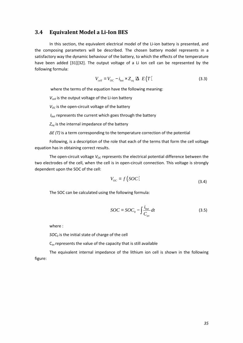
In this section, the equivalent electrical model of the Li-ion battery is presented, and
the composing parameters will be described. The chosen battery model represents in a
satisfactory way the dynamic behaviour of the battery, to which the effects of the temperature
have been added [31][32]. The output voltage of a Li Ion cell can be represented by the
following formula:
( )cell OC bat eqV V i Z E T= − × + ∆
(3.3)
where the terms of the equation have the following meaning:
Vcell is the output voltage of the Li-ion battery
VOC is the open-circuit voltage of the battery
Ibat represents the current which goes through the battery
Zeq is the internal impedance of the battery
ΔE (T) is a term corresponding to the temperature correction of the potential
Following, is a description of the role that each of the terms that form the cell voltage
equation has in obtaining correct results.
The open-circuit voltage VOC represents the electrical potential difference between the
two electrodes of the cell, when the cell is in open-circuit connection. This voltage is strongly
dependent upon the SOC of the cell:
( )OCV f SOC= (3.4)
The SOC can be calculated using the following formula:
0bat
av
iSOC SOC dt
C= − ∫
(3.5)
where :
SOC0 is the initial state of charge of the cell
Cav represents the value of the capacity that is still available
The equivalent internal impedance of the lithium ion cell is shown in the following
figure:
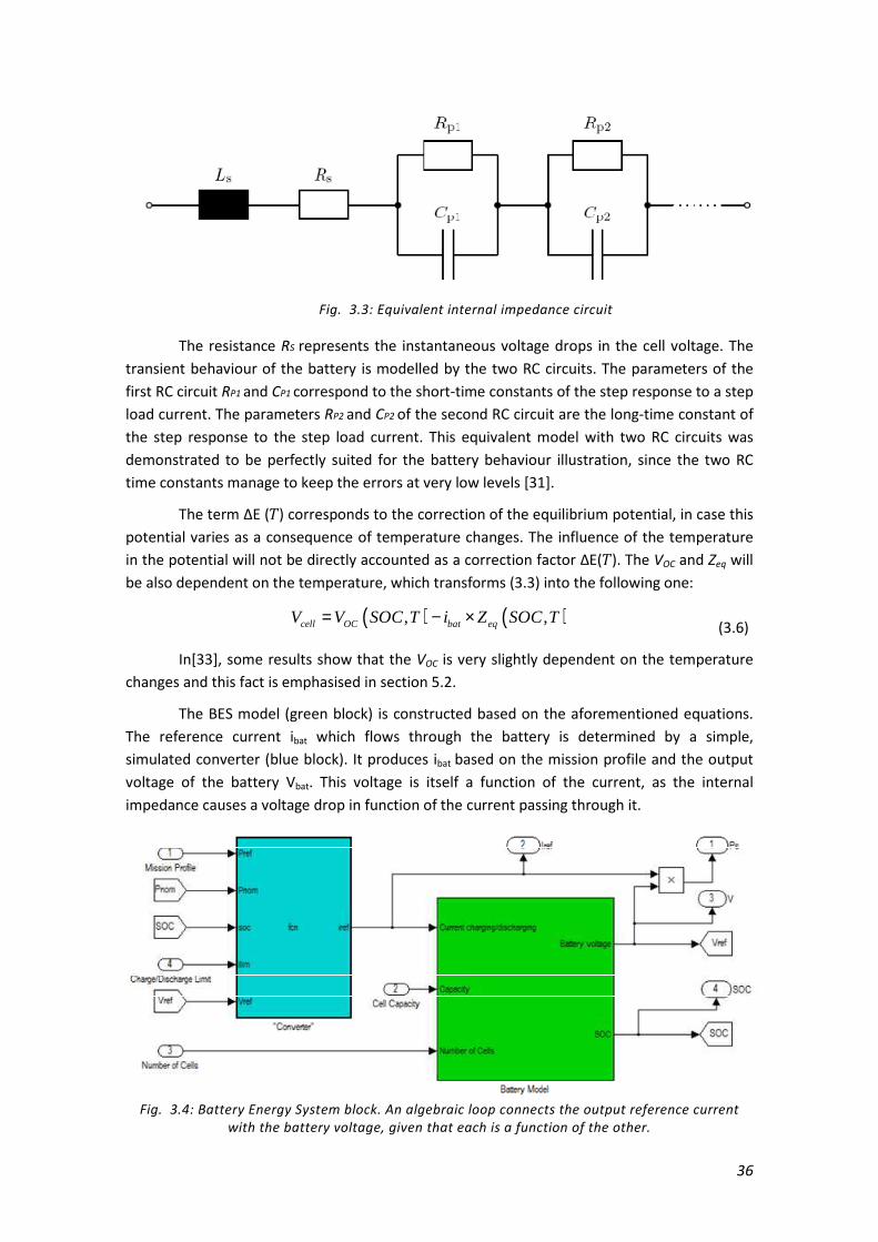
36
Fig. 3.3: Equivalent internal impedance circuit
The resistance RS represents the instantaneous voltage drops in the cell voltage. The
transient behaviour of the battery is modelled by the two RC circuits. The parameters of the
first RC circuit RP1 and CP1 correspond to the short-time constants of the step response to a step
load current. The parameters RP2 and CP2 of the second RC circuit are the long-time constant of
the step response to the step load current. This equivalent model with two RC circuits was
demonstrated to be perfectly suited for the battery behaviour illustration, since the two RC
time constants manage to keep the errors at very low levels [31].
The term ΔE () corresponds to the correction of the equilibrium potential, in case this
potential varies as a consequence of temperature changes. The influence of the temperature
in the potential will not be directly accounted as a correction factor ΔE(). The VOC and Zeq will
be also dependent on the temperature, which transforms (3.3) into the following one:
( ) ( ), ,cell OC bat eqV V SOC T i Z SOC T= − × (3.6)
In[33], some results show that the VOC is very slightly dependent on the temperature
changes and this fact is emphasised in section 5.2.
The BES model (green block) is constructed based on the aforementioned equations.
The reference current ibat which flows through the battery is determined by a simple,
simulated converter (blue block). It produces ibat based on the mission profile and the output
voltage of the battery Vbat. This voltage is itself a function of the current, as the internal
impedance causes a voltage drop in function of the current passing through it.
Fig. 3.4: Battery Energy System block. An algebraic loop connects the output reference current with the battery voltage, given that each is a function of the other.
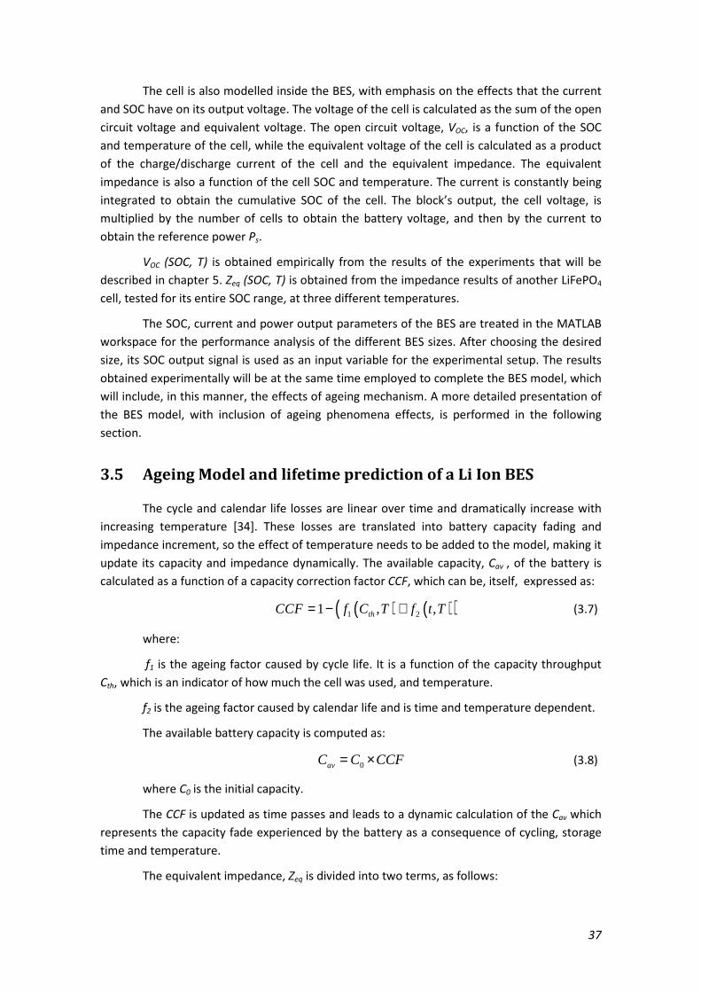
37
The cell is also modelled inside the BES, with emphasis on the effects that the current
and SOC have on its output voltage. The voltage of the cell is calculated as the sum of the open
circuit voltage and equivalent voltage. The open circuit voltage, VOC, is a function of the SOC
and temperature of the cell, while the equivalent voltage of the cell is calculated as a product
of the charge/discharge current of the cell and the equivalent impedance. The equivalent
impedance is also a function of the cell SOC and temperature. The current is constantly being
integrated to obtain the cumulative SOC of the cell. The block’s output, the cell voltage, is
multiplied by the number of cells to obtain the battery voltage, and then by the current to
obtain the reference power Ps.
VOC (SOC, T) is obtained empirically from the results of the experiments that will be
described in chapter 5. Zeq (SOC, T) is obtained from the impedance results of another LiFePO4
cell, tested for its entire SOC range, at three different temperatures.
The SOC, current and power output parameters of the BES are treated in the MATLAB
workspace for the performance analysis of the different BES sizes. After choosing the desired
size, its SOC output signal is used as an input variable for the experimental setup. The results
obtained experimentally will be at the same time employed to complete the BES model, which
will include, in this manner, the effects of ageing mechanism. A more detailed presentation of
the BES model, with inclusion of ageing phenomena effects, is performed in the following
section.
3.5 Ageing Model and lifetime prediction of a Li Ion BES
The cycle and calendar life losses are linear over time and dramatically increase with
increasing temperature [34]. These losses are translated into battery capacity fading and
impedance increment, so the effect of temperature needs to be added to the model, making it
update its capacity and impedance dynamically. The available capacity, Cav , of the battery is
calculated as a function of a capacity correction factor CCF, which can be, itself, expressed as:
( ) ( )( )1 21 , ,thCCF f C T f t T= − +
(3.7)
where:
f1 is the ageing factor caused by cycle life. It is a function of the capacity throughput
Cth, which is an indicator of how much the cell was used, and temperature.
f2 is the ageing factor caused by calendar life and is time and temperature dependent.
The available battery capacity is computed as:
0avC C CCF= ×
(3.8)
where C0 is the initial capacity.
The CCF is updated as time passes and leads to a dynamic calculation of the Cav which
represents the capacity fade experienced by the battery as a consequence of cycling, storage
time and temperature.
The equivalent impedance, Zeq is divided into two terms, as follows:
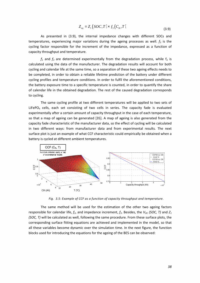
38
( ) ( )1 3, ,eq thZ Z SOC T f C T= × (3.9)
As presented in (3.9), the internal impedance changes with different SOCs and
temperatures, experiencing major variations during the ageing processes as well. f3 is the
cycling factor responsible for the increment of the impedance, expressed as a function of
capacity throughput and temperature.
f1 and f3 are determined experimentally from the degradation process, while f2 is
calculated using the data of the manufacturer. The degradation results will account for both
cycling and calendar life at the same time, so a separation of these two ageing effects needs to
be completed, in order to obtain a reliable lifetime prediction of the battery under different
cycling profiles and temperature conditions. In order to fulfil the aforementioned conditions,
the battery exposure time to a specific temperature is counted, in order to quantify the share
of calendar life in the obtained degradation. The rest of the caused degradation corresponds
to cycling.
The same cycling profile at two different temperatures will be applied to two sets of
LiFePO4 cells, each set consisting of two cells in series. The capacity fade is evaluated
experimentally after a certain amount of capacity throughput in the case of each temperature,
so that a map of ageing can be generated [35]. A map of ageing is also generated from the
capacity fade characteristic of the manufacturer data, so the effect of cycling will be calculated
in two different ways: from manufacturer data and from experimental results. The next
surface plot is just an example of what CCF characteristic could empirically be obtained when a
battery is cycled at different ambient temperatures.
0
2
46
8x 10
4
1020
3040
50
0.6
0.8
1
T (ºC)Cth (Ah)
CC
F
0 1 2 3 4 5x 10
4
0.75
0.8
0.85
0.9
0.95
1
Capacity throughput (Ah)
CC
F
CCF40 vs. Cth fit 40 ºCCCF50 vs. Cth fit 50 ºC
Fig. 3.5: Example of CCF as a function of capacity throughput and temperature.
The same method will be used for the estimation of the other two ageing factors
responsible for calendar life, f2, and impedance increment, f3. Besides, the VOC (SOC, T) and Z1
(SOC, T) will be calculated as well, following the same procedure. From these surface plots, the
corresponding surface fitting equations are achieved and implemented in the model, so that
all these variables become dynamic over the simulation time. In the next figure, the function
blocks used for introducing the equations for the ageing of the BES can be observed:

39
Fig. 3.6: Ageing block of the BES.
As the simulation time passes, the capacity throughput adds up and the ageing cycling
factor f1 experiences a continuous increase. f2 also increases over the time and these two
factors are added in order to obtain the total degradation suffered by the battery. When the
total degradation reaches the level of 20%, which corresponds to the battery end of life, the
simulation time is measured and this will be the indicator of the lifetime of the BES.
The input data available for forecast improvement service simulation corresponds to
one year. The BES may not reach its end of life by this time, so the next years will be
considered to have the same characteristics as the one available, meaning the same capacity
throughput. Taking into account this assumption, the same current profile as in the first year
is applied again several times until the total degradation factor reaches 20%. For this purpose,
an additional and simple lifetime prediction model was implemented, shown in the figure of
appendix C.
The simulation period plays a key role in performing a reliable lifetime prediction of
the BES. For instance, only 43601 points (minutes), corresponding to a single month signal, are
simulated. In case the forecast prediction during this month is much more precise than usual,
the BES would be used less, suffering of a reduced ageing, so the Cth would lower accordingly,
meaning that the calculated lifetime is larger than the real one. In order to avoid these
inconclusive lifetime predictions, a large simulation period is recommended, going up to the
whole year signal available.

40
4 Lithium Iron Phosphate Cell Characterisation
Chapter 4 is dedicated to a detailed description of the laboratory work performed, and
it has as departure point the laboratory setup depiction, followed by a detailed description of
the steps utilised in order to obtain the SOC input signal to the setup, continued with a
description of the testing procedure used. The last part of the chapter contains relevant data
about the Impedance Spectroscopy measurement procedure utilised in order to acquire the
parameters of the battery equivalent model.
4.1 Test object specifications
The tested system was two cells in series which come from a BYD LiFePO4 battery. The
main characteristics of each FV50 LiFePO4 cell are the following:
Basic Characteristics
Nominal Voltage: 3.20 V
Nominal capacity: 50 Ah
Charge Voltage: 3.6±0.49 V
Maximum Charging Current (25 °C):
10 A (Standard)
100 A (Maximum continuous charge)
Discharging cut-off Voltage: 2.00 V
Maximum Discharging Current (25 °C):
10 A (Standard)
500 A (Maximum continuous discharge)
Mechanical Characteristics
Thickness: 28.5 mm
Width: 100.5 mm
Height: 376 mm
Weight: 1900 g
Operating Conditions
Relative Humidity: 5% ÷ 95%
Charge Temperature: 0 ÷ 55 °C
Discharge Temperature: - 25 °C ÷ 55 °C
Storage Temperature: -10 ÷ + 45 °
The tested system is composed of 2 individual cells in series, which are assumed to be
identical. It, therefore, has twice the voltage of one individual cell, but it shares the same
conditions for current and operating points. Measuring a battery’s capacity in ampere hours is
especially practical, since the value holds with changes in voltage. This means that both the 2-
cell module and an individual cell have 50 Ah, only that these 50 Ah translate into around 320
Wh for the whole 2-cell module, and 160 Wh for an individual cell, as their respective voltages
are different.
Laboratory measurements were performed using the following setup:
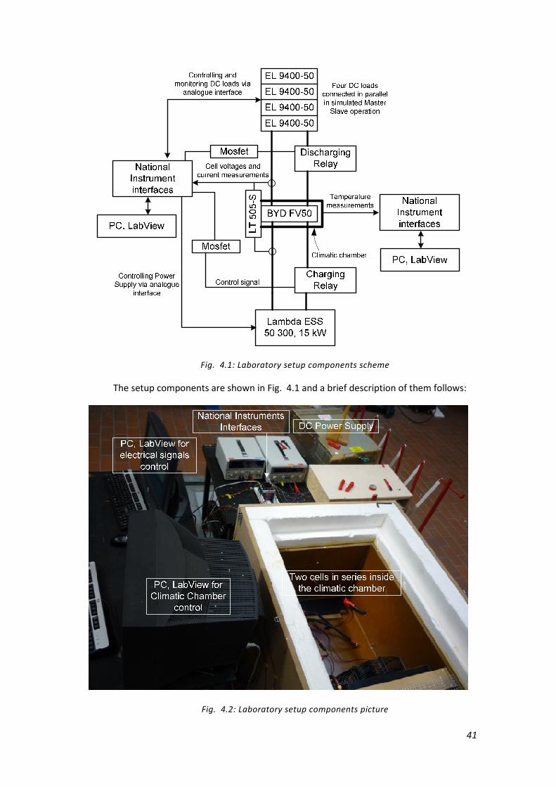
41
Fig. 4.1: Laboratory setup components scheme
The setup components are shown in Fig. 4.1 and a brief description of them follows:
Fig. 4.2: Laboratory setup components picture

42
Lambda ESS 50 V 300A is a DC Power Supply controlled by the analogue interface from
the National Instruments (NI) CompactDAQ chassis. The analogue interface does not allow for
simultaneous control and monitoring of the Power Supply. In order to obtain a correct
charging characteristic, at a precise moment there has to be a switching from the constant
current to the CVOM. In remote control, through the analogue interface, this switching is
performed as follows:
The operating mode of the power supply is determined by the relation between the
control settings and the load resistance. The automatic switching between the modes depends
upon: The load, RL, connected to the terminals of the Power Supply
The front panel voltage control setting, Vset
The front panel current control setting, Iset
The Power Supply does not have an option to calculate the delivered capacity to the
battery. The calculation of the delivered capacity is implemented in LabView.
EL9400-50 2400W electronic DC load: The setup contains four DC loads, connected in
parallel. These DC loads cannot work in real Master Slave operation sharing all the parameters
(voltage, current, power, resistance). Simulated Master Slave operation with current sharing is
employed. The CompactDAQ chassis delivers the current reference through the analogue
interface. The calculation of the capacity delivered from the battery is also performed using
the LabView software [36].
NI (National Instruments) Interfaces: The CompactDAQ chassis was employed in order
to control the setup components and to monitor the parameters of the battery. It was
equipped with two NI 9263 modules for signal generation and one NI 9229 module for
measurement acquisition [36].
Two signals from 0 to 5 V are generated for the Power Supply, which set the charging
current and the voltage at its terminals. One signal from 0 to 10 V goes to the DC Loads to set
the discharging current. Two relays are used for the protection of the battery and to avoid
simultaneous charging and discharging. Because of the insufficient current capability of the
module NI 9263 to close the relays, a Mosfet is used as an actuator. So other two signals of 10
V are generated for supplying the Mosfets between gate and source, so that they can close the
circuit to then close the corresponding charging or discharging relay. These relays are fed by 12
V at their terminals.
Three signals are acquired by the NI 9229 module which are the voltage of each of the
two cells and the voltage drop at the measuring resistance of the transducer, which is used to
calculate the current [36].
Another CompactDAQ chassis was used for the control of the climatic chamber
temperature.
A Current transducer LT 505-S with a conversion ratio 1:5000 is used for the
measurement of the current. The measuring resistance has a value of 50 Ω and a tolerance of
0.01%, so it can be supposed that it is not introducing errors in the measurement of the
current. The calculation of this current is done using the following scaling equation:

43
( / ) 5000MI V R a= × + (4.1)
where I is the charging or discharging current, RM is the measuring resistance, V is the
voltage drop at the RM and a is an independent coefficient which is added to compensate for
the error caused by the inaccuracies of the DC Power Supply and DC Loads. This coefficient is
calculated according to the measurements given by the high accuracy oscilloscope, Yokogawa
Digital Oscilloscope DL9040.
A climatic chamber with temperature control was used for the placement of the cells.
It is a box which has two wooden layers with polystyrene inside for a better thermal isolation.
Three holes were made in the chamber in order to introduce the current and voltage
measurement cables and the thermocouples into it. The two cells were placed on two pieces
of wood, so that one thermocouple could be placed on the bottom of each cell. Thus, these
thermocouples were positioned in such a manner that the air flow around them is reduced.
Other three thermocouples were located at three different heights and sides of the chamber.
They were used for the calculation of the ambient temperature of the chamber, as an average
of the three of them, and as an input for the temperature control programme made in
LabView.
As can be seen in Fig. 4.3, an initial test was done in order to see how much time the
chamber needed to heat up from 20 to 40 °C. The time needed to reach a value close to 40 °C
was 25 minutes and after 35 minutes, the temperature stabilised around 40 °C.
Fig. 4.3: Temperature variation when heating the climatic chamber from 20 to 40 °C
4.1.1 Description of the used programme
The software used for the acquisition of the parameter measurements and the control
signal generation is LabView. A programme created in this software was used for monitoring
the measurements of the voltage of each cell and the charging/discharging current. The
sampling time used was 0.5 s, because a large number of cycles in the input profile had a quite
short duration, so a better precision of the DOD of each of them could be achieved.
These measurements are also suitable for the protection of the cells. If the voltage of
one of the two cells is lower than 2 V, which is the minimum corresponding to the fully
discharged state, or higher than 3.587 V, which is the maximum corresponding to the fully
0000 500500500500 1000100010001000 1500150015001500 200020002000200020202020
25252525
30303030
35353535
40404040
45454545
Time (s)
T (
ºC)
1400140014001400 1600160016001600 1800180018001800 2000200020002000 2200220022002200 2400240024002400
39.439.439.439.4
39.639.639.639.6
39.839.839.839.8
40404040
40.240.240.240.2

44
charged state, the programme gives a signal for the opening (meaning setup disconnection) of
both relays. The other condition that could be set in the programme for circuit disconnection
was for the charging current to reach to a value lower than 2 A, which means that the cells are
totally charged. This last kind of protection was not implemented, because of the possible
difference in the voltage of each cell, which can lead to the overcharging of one of them. When
charging, the charging relay is closed and the discharging relay opened. When discharging, the
opposite happens. A screenshot of the Graphical User Interface can be seen in the next figure.
Fig. 4.4: Screenshot of the Graphical User Interface and Block Diagramme of LabView programme
The programme calculates the capacity of the cells (Ah) by integration of the
charging/discharging current over time. In case of discharge, it was considered that the current
takes negative values, so the delivered capacity is also negative. The SOC, which is expressed in
percentages, is calculated as the acquired capacity of the battery over its total capacity.
Another programme, contained in another PC, was used for acquiring the
measurements of the ambient temperature and of the temperature on the surface of each
cell. The sampling time for this programme was set to 1 second.
4.2 Testing current profile generation
In this section, the results of the simulation for different sizes of storage are analysed,
in order to select a current profile which will be used as input for the cell experiments. The
simulation performs an improvement of the wind power forecast prediction, as well as a
gradient reduction, taking into account the current demands for wind power integration,
stipulated in the German Grid codes, which is a maximum allowed variation of 10% of the
nominal power per minute. The gradient reduction is very permissive and, in comparison with
the forecast improvement, it is not so demanding for the BES, meaning that the stress levels
on the BES are quite small.
The next graph emphasizes the Average Normalised Mean Absolute Error reduction for
half an hour and one hour of duration and different storage power, where 1 p.u. corresponds
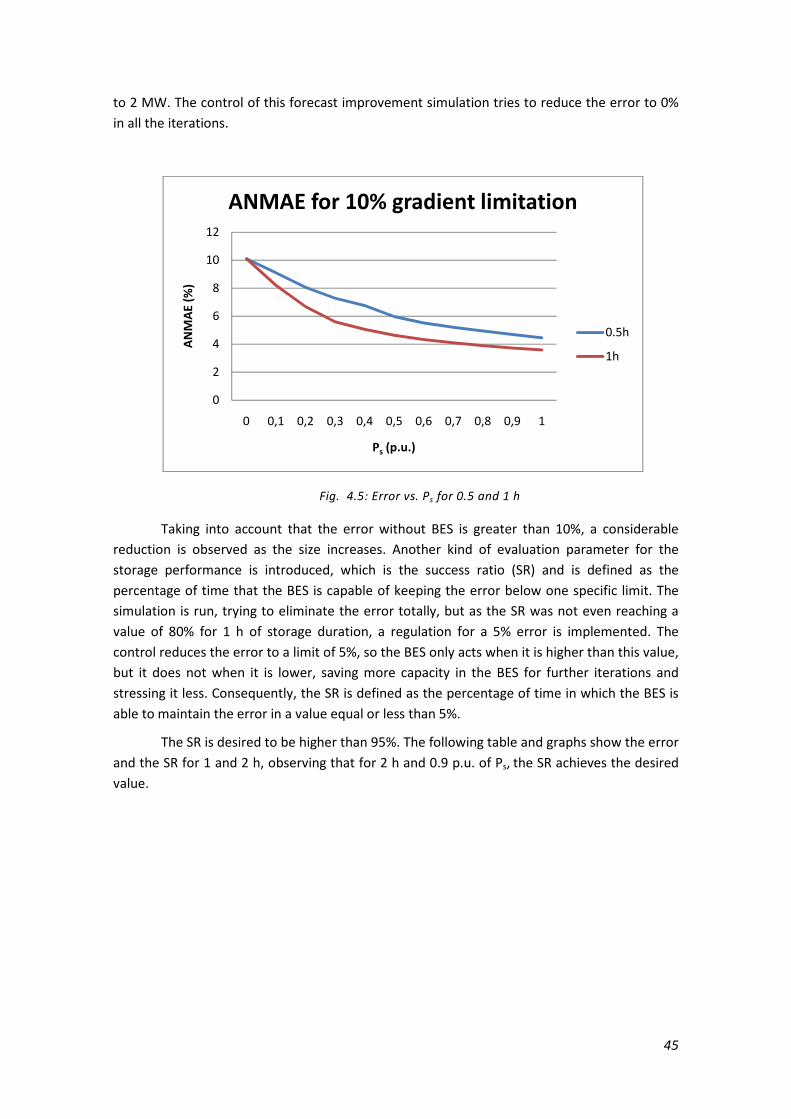
45
to 2 MW. The control of this forecast improvement simulation tries to reduce the error to 0%
in all the iterations.
Fig. 4.5: Error vs. Ps for 0.5 and 1 h
Taking into account that the error without BES is greater than 10%, a considerable
reduction is observed as the size increases. Another kind of evaluation parameter for the
storage performance is introduced, which is the success ratio (SR) and is defined as the
percentage of time that the BES is capable of keeping the error below one specific limit. The
simulation is run, trying to eliminate the error totally, but as the SR was not even reaching a
value of 80% for 1 h of storage duration, a regulation for a 5% error is implemented. The
control reduces the error to a limit of 5%, so the BES only acts when it is higher than this value,
but it does not when it is lower, saving more capacity in the BES for further iterations and
stressing it less. Consequently, the SR is defined as the percentage of time in which the BES is
able to maintain the error in a value equal or less than 5%.
The SR is desired to be higher than 95%. The following table and graphs show the error
and the SR for 1 and 2 h, observing that for 2 h and 0.9 p.u. of Ps, the SR achieves the desired
value.
0
2
4
6
8
10
12
0 0,1 0,2 0,3 0,4 0,5 0,6 0,7 0,8 0,9 1
AN
MA
E (
%)
Ps (p.u.)
ANMAE for 10% gradient limitation
0.5h
1h
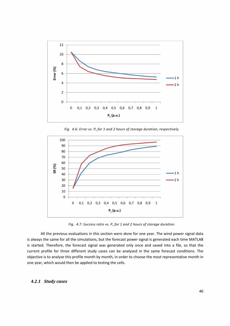
46
Fig. 4.6: Error vs. Ps for 1 and 2 hours of storage duration, respectively.
Fig. 4.7: Success ratio vs. Ps for 1 and 2 hours of storage duration.
All the previous evaluations in this section were done for one year. The wind power signal data
is always the same for all the simulations, but the forecast power signal is generated each time MATLAB
is started. Therefore, the forecast signal was generated only once and saved into a file, so that the
current profile for three different study cases can be analysed in the same forecast conditions. The
objective is to analyse this profile month by month, in order to choose the most representative month in
one year, which would then be applied to testing the cells.
4.2.1 Study cases
0
2
4
6
8
10
12
0 0,1 0,2 0,3 0,4 0,5 0,6 0,7 0,8 0,9 1
Err
or
(%)
Ps (p.u.)
1 h
2 h
0
10
20
30
40
50
60
70
80
90
100
0 0,1 0,2 0,3 0,4 0,5 0,6 0,7 0,8 0,9 1
SR
(%
)
Ps (p.u.)
1 h
2 h

47
The simulation is analysed for three different BES sizes, evaluating its behaviour for each of the
twelve months of a year and also the complete year, emphasized in the last part of the graph. The first
size chosen is 1 p.u. and 2 hours, as in this case the average value of the SR is situated above 85 %
meaning that in 85 % of the time in 1 year the error between the wind power forecast and the actual
wind power production was below 5 %. This value of the success ratio was considered as being good
enough for evaluation of the Forecast Improvement service. The power of the BES considered in the first
study case is decremented by a factor of 5 and the energy of the BES increased by the same factor in
order to maintain the same overall power flow possibilities of the BES, giving rise to the second battery
storage size of 0.2 p.u. in the case of Ps and 10 hours of Ps available in case of Es. This new BES gives also
the possibility to visualise possible differences in the current rates. A third size, represented in the graph
in green, fulfils the condition of having a SR higher than 90% for each single month, and for the whole
year.
The error, success ratio, rest time and 100% DOD equivalent number of cycles for the three
different BES sizes are presented in the next figures.
Fig. 4.8: Error analysis for the three study cases
3
3,5
4
4,5
5
5,5
Error (%)
1 p.u. - 2 h
0.2 p.u. - 10 h
0.95 p.u. - 6 h
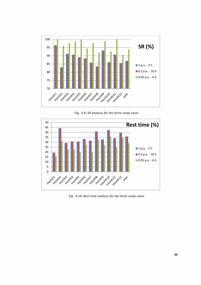
48
Fig. 4.9: SR analysis for the three study cases
Fig. 4.10: Rest time analysis for the three study cases
70
75
80
85
90
95
100
SR (%)
1 p.u. - 2 h
0.2 p.u. - 10 h
0.95 p.u. - 6 h
0
5
10
15
20
25
30
35
40
45
50Rest time (%)
1 p.u. - 2 h
0.2 p.u. - 10 h
0.95 p.u. - 6 h
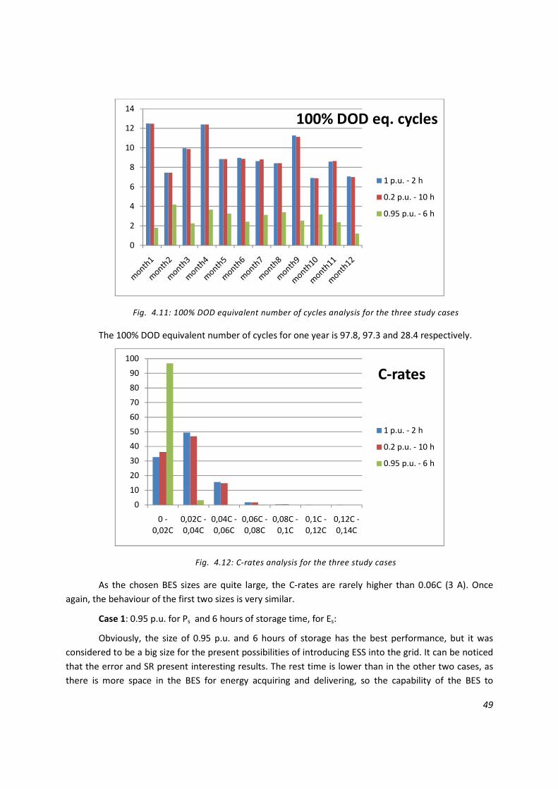
49
Fig. 4.11: 100% DOD equivalent number of cycles analysis for the three study cases
The 100% DOD equivalent number of cycles for one year is 97.8, 97.3 and 28.4 respectively.
Fig. 4.12: C-rates analysis for the three study cases
As the chosen BES sizes are quite large, the C-rates are rarely higher than 0.06C (3 A). Once
again, the behaviour of the first two sizes is very similar.
Case 1: 0.95 p.u. for Ps and 6 hours of storage time, for Es:
Obviously, the size of 0.95 p.u. and 6 hours of storage has the best performance, but it was
considered to be a big size for the present possibilities of introducing ESS into the grid. It can be noticed
that the error and SR present interesting results. The rest time is lower than in the other two cases, as
there is more space in the BES for energy acquiring and delivering, so the capability of the BES to
0
2
4
6
8
10
12
14
100% DOD eq. cycles
1 p.u. - 2 h
0.2 p.u. - 10 h
0.95 p.u. - 6 h
0
10
20
30
40
50
60
70
80
90
100
0 -
0,02C
0,02C -
0,04C
0,04C -
0,06C
0,06C -
0,08C
0,08C -
0,1C
0,1C -
0,12C
0,12C -
0,14C
C-rates
1 p.u. - 2 h
0.2 p.u. - 10 h
0.95 p.u. - 6 h

50
maintain the error below the limit of 5% is higher. The BES acts more time (higher cycling time), trying to
eliminate the differences between the actual wind power generation and the previously predicted one.
Due to this fact, it could be assumed that the BES suffers of more degradation for this big size, but as can
be seen in Fig. 4.11, the number of 100% DOD equivalent cycles is greatly diminished compared to the
other two, relatively, small storages. Besides, the C-rates are lower for this BES size.
Case 2: 0.2 p.u. for Ps and 10 hours of storage time, in the case of Es:
This storage size is able to store the same amount of energy as the one of 1 p.u. and 2 hours of
storage. That is why all the results are very similar to it. However, it was desired to analyse it in order to
check if t differences in the C-rates, compared to the first study case, are noticeable. They are also very
similar, so the current profile was not acquired from this study case.
Case 3: 1 p.u. for Ps and 2 hours of storage time:
In Fig. 4.9 can be seen that this size is the one which achieves an acceptable value of the SR,
compared to its size. This is the main reason why it is chosen to generate the current profile which will
be used for the experiment, although the success ratio is lower than 90% for the entire year, because
the input forecast signal seems to be overestimated. A proof is the fact that even for a BES as big as 1.5
p.u. for the storage power and an energy storage of 8 hours of maximum storage power, the target of
95 % for the SR cannot be achieved.
The current profile coming from the simulation for 1 p.u. and 2 hours of storage is shown in the
next figure and it is subject to a detailed analysis, performed in Table 4.1. The zero current points, where
the BES is in resting mode, are removed from the signal in order to speed up the testing process.
Fig. 4.13: Current profile
The first two columns point out how many cycles are present in intervals of 5% DOD. The
average DOD of all these cycles is calculated for each interval. As the C-rates are very low, it was decided
to speed up the testing procedure by increasing the C-rate to 2C (100 A), so the influence of the
magnitude of these currents in the degradation process is neglected. The actual test time represents
how much time is needed to charge/discharge the total number of cycles of their respective average
0000 0.50.50.50.5 1111 1.51.51.51.5 2222 2.52.52.52.5 3333 3.53.53.53.5 4444 4.54.54.54.5 5555
x 10x 10x 10x 105555
-10-10-10-10
-8-8-8-8
-6-6-6-6
-4-4-4-4
-2-2-2-2
0000
2222
4444
6666
8888
10101010
Number of points
Cur
rent
(A
)
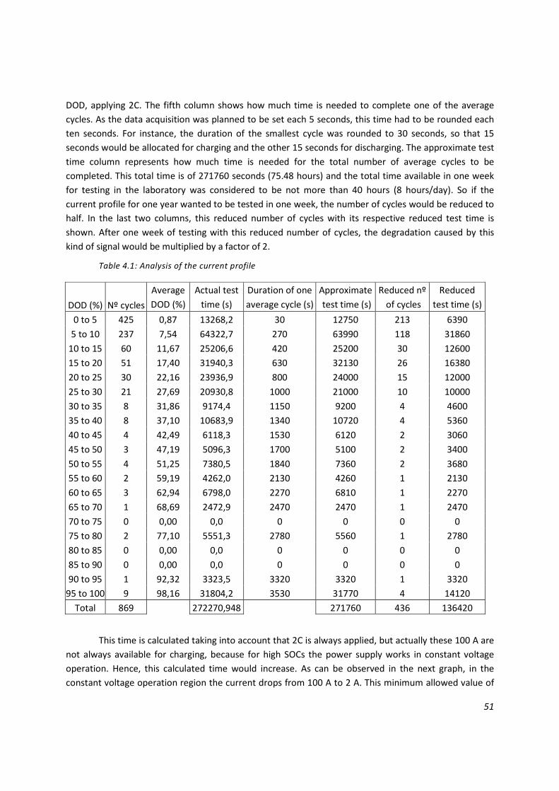
51
DOD, applying 2C. The fifth column shows how much time is needed to complete one of the average
cycles. As the data acquisition was planned to be set each 5 seconds, this time had to be rounded each
ten seconds. For instance, the duration of the smallest cycle was rounded to 30 seconds, so that 15
seconds would be allocated for charging and the other 15 seconds for discharging. The approximate test
time column represents how much time is needed for the total number of average cycles to be
completed. This total time is of 271760 seconds (75.48 hours) and the total time available in one week
for testing in the laboratory was considered to be not more than 40 hours (8 hours/day). So if the
current profile for one year wanted to be tested in one week, the number of cycles would be reduced to
half. In the last two columns, this reduced number of cycles with its respective reduced test time is
shown. After one week of testing with this reduced number of cycles, the degradation caused by this
kind of signal would be multiplied by a factor of 2.
Table 4.1: Analysis of the current profile
Average Actual test Duration of one Approximate Reduced nº Reduced
DOD (%) Nº cycles DOD (%) time (s) average cycle (s) test time (s) of cycles test time (s)
0 to 5 425 0,87 13268,2 30 12750 213 6390
5 to 10 237 7,54 64322,7 270 63990 118 31860
10 to 15 60 11,67 25206,6 420 25200 30 12600
15 to 20 51 17,40 31940,3 630 32130 26 16380
20 to 25 30 22,16 23936,9 800 24000 15 12000
25 to 30 21 27,69 20930,8 1000 21000 10 10000
30 to 35 8 31,86 9174,4 1150 9200 4 4600
35 to 40 8 37,10 10683,9 1340 10720 4 5360
40 to 45 4 42,49 6118,3 1530 6120 2 3060
45 to 50 3 47,19 5096,3 1700 5100 2 3400
50 to 55 4 51,25 7380,5 1840 7360 2 3680
55 to 60 2 59,19 4262,0 2130 4260 1 2130
60 to 65 3 62,94 6798,0 2270 6810 1 2270
65 to 70 1 68,69 2472,9 2470 2470 1 2470
70 to 75 0 0,00 0,0 0 0 0 0
75 to 80 2 77,10 5551,3 2780 5560 1 2780
80 to 85 0 0,00 0,0 0 0 0 0
85 to 90 0 0,00 0,0 0 0 0 0
90 to 95 1 92,32 3323,5 3320 3320 1 3320
95 to 100 9 98,16 31804,2 3530 31770 4 14120
Total 869
272270,948
271760 436 136420
This time is calculated taking into account that 2C is always applied, but actually these 100 A are
not always available for charging, because for high SOCs the power supply works in constant voltage
operation. Hence, this calculated time would increase. As can be observed in the next graph, in the
constant voltage operation region the current drops from 100 A to 2 A. This minimum allowed value of

52
current indicates that the cell is totally charged, so the protections of the setup must act in order to
avoid overcharging of the cell.
Fig. 4.14: Constant voltage operation analysis
When the constant voltage operation starts, the voltage at the terminals of the cell is 3.464 V.
Taking into account that the voltage set at the terminals of the power supply is 3.6 V, the voltage drop
on the current cables is 0.136 V. Their resistance can be calculated as this voltage drop over the current,
which is 50 A. Therefore, the resistance of the cables is approximately 2.72 mΩ. When the cells are new,
the constant voltage operation starts at high SOC, but as they are facing degradation, their charging
voltage characteristic rises up, thus this operation starts at earlier SOC.
Another issue comes up after all this testing procedure calculation which is the sequence of the
cycles applied. The negligence of this sequence would cause a different degradation in the BES, so a
different way of testing turns out to be of a higher interest. The SOC signal, obtained after applying the
Rainflow cycle counting method to the SOC of the simulation, is thought to be a more precise testing
profile for the experiment. The next figure presents the SOC profile used for the battery ageing tests. As
in the current profile, the stationary points are also removed from the signal in such a manner that the
testing profile contains no consecutive points with the same SOC.
0 500 1000 1500 2000 2500 3000
2.8
3
3.2
3.4
3.6
Time (s)
Vol
tage
(V
)
0 500 1000 1500 2000 2500 30000
20
40
60
Cur
rent
(A
)

53
Fig. 4.15: SOC testing profile.
The limits of 10% and 90% for the SOC profile are set due to mainly three reasons:
Weekly degradation:
The capacity tests and impedance measurements for each cell are carried out periodically, so
the capacity decreases along the week while the SOC in the testing program is calculated having the
capacity measurement available at the beginning of the week. For instance, if the cell capacity
decreased 4% during the testing week, it would mean that the testing limits for the SOC should be set to
2% and 98%. Ignoring these limits, the setup would be unexpectedly stopped when desiring to reach low
or high SOCs. After each new capacity test, the SOC calculation is based on this new value.
DC loads limitation:
The DC loads are able to discharge at 100 A when the voltage at the terminals of the two cells is
higher than 4.66 V, so the minimum voltage set for each cell is 2.33 V. From this value to the minimum
of 2 V, which means the cells are totally discharged, around 0.4 Ah of capacity is not used, so almost 1%
more must be added to these limits. Another possible solution would be to decrease the discharging
current, but that means to increase the testing time, which is not desirable.
Scaling inaccuracy:
The accuracy of the measurement of the current has been proved to be a major issue. The
scaling equation for its calculation has to be different in case of charging or discharging, as different
devices with different precisions are used. A high accuracy oscilloscope, Yokogawa Digital Oscilloscope
DL9040, was used for the estimation of the independent coefficient, which was added to the scaling
equation, although some error is introduced. This error, which is cumulating over time, drives to a
disconnection of the setup.
For instance, if a good measurement of the discharging current is achieved, but more charging
current is measured by the LabView program than it actually flows in the circuit, the consequence can
be seen in the following figure.
0000 200200200200 400400400400 600600600600 800800800800 1000100010001000 1200120012001200 1400140014001400 16001600160016000000
10101010
20202020
30303030
40404040
50505050
60606060
70707070
80808080
90909090
100100100100
Number of points
SO
C (
%)
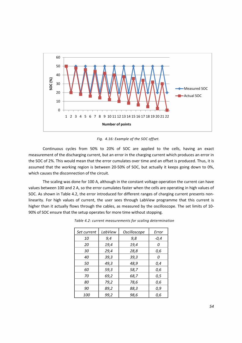
54
Fig. 4.16: Example of the SOC offset.
Continuous cycles from 50% to 20% of SOC are applied to the cells, having an exact
measurement of the discharging current, but an error in the charging current which produces an error in
the SOC of 2%. This would mean that the error cumulates over time and an offset is produced. Thus, it is
assumed that the working region is between 20-50% of SOC, but actually it keeps going down to 0%,
which causes the disconnection of the circuit.
The scaling was done for 100 A, although in the constant voltage operation the current can have
values between 100 and 2 A, so the error cumulates faster when the cells are operating in high values of
SOC. As shown in Table 4.2, the error introduced for different ranges of charging current presents non-
linearity. For high values of current, the user sees through LabView programme that this current is
higher than it actually flows through the cables, as measured by the oscilloscope. The set limits of 10-
90% of SOC ensure that the setup operates for more time without stopping.
Table 4.2: current measurements for scaling determination
Set current LabView Oscilloscope Error
10 9,4 9,8 -0,4
20 19,4 19,4 0
30 29,4 28,8 0,6
40 39,3 39,3 0
50 49,3 48,9 0,4
60 59,3 58,7 0,6
70 69,2 68,7 0,5
80 79,2 78,6 0,6
90 89,2 88,3 0,9
100 99,2 98,6 0,6
0
10
20
30
40
50
60
1 2 3 4 5 6 7 8 9 10 11 12 13 14 15 16 17 18 19 20 21 22
SO
C (
%)
Number of points
Measured SOC
Actual SOC

55
Delay in data acquisition
As the SOC profile has many small DOD cycles, the data acquisition was taken each 0.5 s, so that
these cycles could be accomplished. After observing that the setup suffered many disconnections in
short periods of testing, it was cleared that the scaling inaccuracy was not the main reason of it.
LabView programme was not calculating the exact capacity that was delivered or acquired by the cells.
Apparently, the data acquisition had a delay of 0.125 s, transforming the data acquisition time into 0.625
s, instead of the chosen 0.5 s. Thus, LabView was giving a capacity calculated in intervals of time of 0.5 s,
when the actual interval was larger. That means less capacity was seeing by the user (in blue) and
therefore, bigger cycles (in red) were applied to the cells. The actual capacity was calculated using Excel.
Fig. 4.17: Capacity measurement verification
In the above figure, the consequence of the delay in the data acquisition can be observed. This
measurement error does not cause a displacement of the operating region, as in the case of the scaling
inaccuracy issue, but bigger cycles than desired were applied to the cells. After a big cycle, the error
cumulated over the time causing the tripping of the protection relays. Although zero capacity was
supposed to be in the cells, 0.8 Ah were still remaining. Around 0.4 Ah is due to the disconnection of the
cells at 2.33 V (DC loads limitation) and the other 0.4 Ah is due to the scaling error, which was caused
after 3 hours of testing.
4.3 The Testing Procedure
As mentioned in a previous section, instead of directly applying the actual values of the currents
obtained for the implemented study case (1 p.u. for Ps and 2 hours of Ps, in case of Es), the applied
testing current was of 100 A, both for charging and discharging, current corresponding to a 2C rate in
case of the studied battery. This augmented was one of the accelerated factors applied in the testing
process. The other accelerating factor was the ambient temperature of the climatic chamber, which was
set to two different high values during the testing process. The main reason for employing the
0 1000 2000 3000 4000 5000 6000 7000 8000 9000 100000
5
10
15
20
25
30
35
40
45
Time (s)
C (
Ah)
LabViewExcel

56
accelerated ageing testing approach was the limited time interval available for completion of the
present study. Normal testing conditions, as the ones obtained from the simulation file would require
the same testing time availability as the one set in the simulation (1 year), time that, as mentioned, was
unavailable. By applying the increased C-rate, the time required to test the input SOC signal
corresponding to an entire year of simulation is reduced was reduced to less than 10 days of testing. The
augmented testing temperatures were employed in order to obtain an increased degradation of the
cells, besides the degradation caused by the high testing C-rate.
The first half of the testing time was dedicated to test a group of two LiFePO4 cells placed in
series under the 2C current rate and the chamber ambient temperature of 50 °C, while the second part
of the testing process was performed with another group of two cells of the same type, at the chamber
ambient temperature of 40 °C.
The applied testing procedure, for both testing temperatures, consisted of the following steps:
• The chamber was heated up to the testing temperature
• The temperature was left to stabilise for a couple of minutes around the testing value
• The setup was started and the cells were charged and discharged to the SOC values
corresponding to the input signal obtained from the simulation file, with a constant current of
100 A
• At the end of each testing day the chamber was opened in order for the cells to reach to the
ambient temperature by the beginning of the next testing day.
These four steps were repeated every testing day. Periodically, two types of tests were
performed in order to assess the cell degradation. The first test performed is the capacity test, which
evaluates the degradation measured as a reduction in the cell capacity during the testing period. The
second type of test used to evaluate the ageing of the cells is the impedance test which evaluates the
increase in cell impedance, responsible for the power fade mechanism. After performing these two
types of cell performance evaluation, the testing was continued. The input SOC signal corresponding to
one year of simulation contains 1743 points, while the testing was continued until approximately 1950
points were tested for each considered temperature, meaning more than one year of simulation in eacjh
case.
4.4 Electrochemical Impedance Spectroscopy
As mentioned in a previous paragraph, in order to properly characterize the behaviour of
rechargeable batteries, an equivalent battery model needs to be constructed. This equivalent
impedance circuit is composed of electrical elements, each of them representing one of the physical
phenomena which are occurring during the functioning of the battery. The determination of the values
of the electrical parameters is vital for the assessment of the battery characteristics and for a proper
understanding of the battery operation.
57
The procedure employed for acquiring the parameters (resistances, capacitances)
consists of performing an impedance sweep on a large frequency range, starting with high frequencies,
ranging around the order of kilohertz or tens of kilohertz and going until values of milihertz. This
procedure is named Electrochemical Impedance Spectroscopy and is being performed for several states
of charge at three different temperatures (25, 35 and 45 °C).Based on the obtained impedance spectra,
the values of the parameters of the studied battery are acquired by applying a Complex Nonlinear Least
Square (CNLS) fitting to each impedance curve. Then, by means of another fitting, the equations
representing each parameter of the equivalent battery model as a function of SOC and temperature are
being attained.
4.4.1 General description of the Electrochemical Impedance Spectroscopy process
Impedance Spectroscopy is a measurement procedure utilized in the determination of the
transfer function of a system in the frequency domain. In case of an electrical system, the transfer
function is the impedance, Z(ω), which relates the input parameter, I(ω) to the output of the system,
U(ω).
As previously mentioned, one of the main conveniences that this procedure brings is the
possibility to provide, in the case of electrochemical systems, the values of the lumped parameters that
form the equivalent impedance model of the system. Each of these parameters has a correspondence in
the physical processes occurring inside the battery during its use.
The procedure consists of applying a sinusoidal current or voltage to the system on a large
frequency range, in order to acquire a continuous spectrum, and measuring the amplitude and phase
shift of the output signal. One of the main problems related to the electrochemical systems is
represented by their nonlinearity. This means that there is no clear relationship between the charge or
discharge current and their voltage output. Another problem arising from their operation is related to
their asymmetry, which means different values of voltage during charge and discharge for the same
value of the applied current. These reasons call for a new parameter, named small-signal resistance,
defined as the slope of the voltage-current characteristic.
( )dU
R R IdI
= = (4.2)
In case of nonlinear the value of this resistance differs of the large signal resistance, RLS.
In order to perform the impedance spectroscopy measurement linearity is required, since the
Fourier transform employed in the measurement process is only applicable to linear systems. Another
stringent demand of the measuring procedure is the application of a sufficiently small excitation signal
as input to the system, resulting in a high precision of the small signal impedance.
One of the main disturbing factors present in the measurement is the harmonics of the
measured frequency, which cause a pronounced altering of the measured signal. Noise is another cause
of distortion of the output signal of the device under test. One effective way of mitigating the negative
impact of the harmonics on the obtained output is the performing of a Discrete Fourier Transform, by
extracting them from the signal [37].

58
4.4.2 Impedance Spectroscopy Measurement Procedure
The impedance spectroscopy measurements were performed with the TrueData-EIS, a high
current impedance meter, operational with a maximum DC current of 1000 A. This measurement device
is intended for measurements of fuel cells and batteries. Its mode of operation is the galvanostatic
mode, meaning applying a sinusoidal current to the device under test (DUT) and acquiring the voltage
response from it. By carrying out a precise control of the values of the input current, the output value of
DUT’s voltage can be taken to desired values.
The frequency range which defines the TrueData-EIS meter operation is between 100 kHz and
200 µHz. The impedance meter contains 36 channels, giving the possibility of performing measurements
of several devices in the same time [38].
The impedance spectroscopy measurement procedure comprises two steps. The first one refers
to bringing the DUT to a quasi stationary condition of the operating point. This means bringing the
battery to the desired temperature level, which will be kept constant during the entire period of the
measurement, and setting the state of charge of the system to a constant value. After completion of
these two operations, the DUT is left to settle for a certain period of time, in order for it to achieve a
dynamic equilibrium state, necessary for a constant operating point. Keeping the operating point
constant implies applying a sufficiently small excitation current on the battery. Still, by performing this
operation, the SOC of the battery can be kept at a constant SOC for a limited period of time, time which
defines the lower frequency limit of the measurement.
The second part of the impedance spectroscopy procedure is represented by the measurement
itself, which is performed by the spectrometer starting with the highest frequency and decreasing the
frequency logarithmically to the lowest value. The number of frequency steps can be specified by the
user, but generally eight to ten frequencies are taken on each decade. The obtained voltage output is
converted by means of a Fourier transform, and the real and imaginary parts of the impedance at
fundamental frequency are used, together with the input current, to determine the value of the
impedance.
As mentioned in a previous paragraph, the harmonics and noise present in measurement can
have a major influence on its precision. Besides the use of a Discrete Fourier Transform in order to
minimize the negative impact of harmonics, a proper connection of the DUT can accentuate the
mitigation of these negative factors. The connection leads are a source of magnetic loops, especially at
higher frequencies. The main element susceptible of introducing errors in the impedance measurement
is represented by the sense cable between the battery and measuring device. The reasons for this
harmful impact on the measurement can be synthesized as follows:
• Occurrence of coupling effects at high frequencies and low impedances between the load
cable and the sense cable
• The sense cable behaves similarly to an antenna which suffers of electromagnetic
interferences
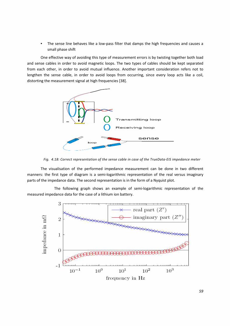
59
• The sense line behaves like a low-pass filter that damps the high frequencies and causes a
small phase shift
One effective way of avoiding this type of measurement errors is by twisting together both load
and sense cables in order to avoid magnetic loops. The two types of cables should be kept separated
from each other, in order to avoid mutual influence. Another important consideration refers not to
lengthen the sense cable, in order to avoid loops from occurring, since every loop acts like a coil,
distorting the measurement signal at high frequencies [38].
Fig. 4.18: Correct representation of the sense cable in case of the TrueData-EIS impedance meter
The visualisation of the performed impedance measurement can be done in two different
manners: the first type of diagram is a semi-logarithmic representation of the real versus imaginary
parts of the impedance data. The second representation is in the form of a Nyquist plot.
The following graph shows an example of semi-logarithmic representation of the
measured impedance data for the case of a lithium ion battery.
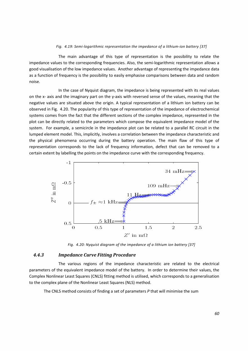
60
Fig. 4.19: Semi-logarithmic representation the impedance of a lithium-ion battery [37]
The main advantage of this type of representation is the possibility to relate the
impedance values to the corresponding frequencies. Also, the semi-logarithmic representation allows a
good visualisation of the low impedance values. Another advantage of representing the impedance data
as a function of frequency is the possibility to easily emphasise comparisons between data and random
noise.
In the case of Nyquist diagram, the impedance is being represented with its real values
on the x- axis and the imaginary part on the y-axis with reversed sense of the values, meaning that the
negative values are situated above the origin. A typical representation of a lithium ion battery can be
observed in Fig. 4.20. The popularity of this type of representation of the impedance of electrochemical
systems comes from the fact that the different sections of the complex impedance, represented in the
plot can be directly related to the parameters which compose the equivalent impedance model of the
system. For example, a semicircle in the impedance plot can be related to a parallel RC circuit in the
lumped element model. This, implicitly, involves a correlation between the impedance characteristic and
the physical phenomena occurring during the battery operation. The main flaw of this type of
representation corresponds to the lack of frequency information, defect that can be removed to a
certain extent by labelling the points on the impedance curve with the corresponding frequency.
Fig. 4.20: Nyquist diagram of the impedance of a lithium ion battery [37]
4.4.3 Impedance Curve Fitting Procedure
The various regions of the impedance characteristic are related to the electrical
parameters of the equivalent impedance model of the battery. In order to determine their values, the
Complex Nonlinear Least Squares (CNLS) fitting method is utilised, which corresponds to a generalisation
to the complex plane of the Nonlinear Least Squares (NLS) method.
The CNLS method consists of finding a set of parameters P that will minimise the sum

61
2
1
( ) ( )M
j j jj
S P Y YC Pω=
= − ∑ (4.3)
where:
M represents the total number of data points
ωj is the weight corresponding to the jth data point
Yj is the jth data point value that has to be fitted
CYj is the jth value of the fitting function, obtained with the parameters P
The fitting of complex data is done by using an array that has twice the number of data points,
in which the first point is the real value of the first data point, while the M+1th point of the array contains
the imaginary value of the first data point. In case of nonlinear systems the fitting process involves
iterations.
The weighting factor ωj is obtained from the relation:
( )1
j RW jω =
(4.4)
The programme LEVM, utilised in the present project in order to perform the CNLS
fitting, contains a variety of ways to calculate RW(j) [39].
The first step used by the LEVM fitting programme is the data initialisation. The
Impedance data points obtained after performing the impedance spectroscopy measurement have to be
organised in three columns in a file which represents the bottom part of the input file used by the
programme to determine the parameters of the fitting function. The first column contains the values of
the frequency, the second column comprises the real values of the impedance at the considered data
points, while the third column, the imaginary part of the impedance.
The LEVM programme incorporates a number of 13 complex fitting circuit models,
ranked from A to R, each of them containing a different topology of electrical elements: resistances,
capacitances, inductances, series and parallel RC circuits and, also, several elements labelled with the
generic name of distributed elements, DE. Some particular types of DE, frequently utilised in curve
fitting of electrochemical systems are the Constant Phase Element (CPE), the ZARC-Cole(ZC) Element and
the Generalized Finite Warburg Impedance.
The Constant Phase Element is a simple distributed element which gives an impedance
with a constant phase angle in the complex plane. This element is incorporated into a topology
comprising a series RC circuit in parallel with the CPE inside the programme, as can be seen in Fig. 4.21.
In case the value of the exponent PHI is set to 1, the CPE has the meaning of a capacitance in the circuit.
The user has the possibility to choose two circuit topologies: the first one incorporating only the CPE,
with the values of the series RC elements set to zero (which means that is not taken into account in the
circuit), and the second topology, the resistance in parallel with the CPE only with the capacitance set to
zero. In this last case the CPE acts like a capacitance.
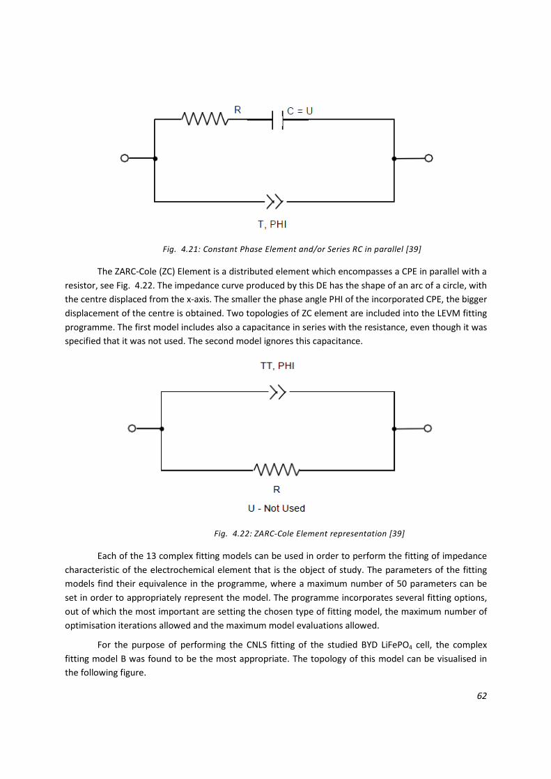
62
Fig. 4.21: Constant Phase Element and/or Series RC in parallel [39]
The ZARC-Cole (ZC) Element is a distributed element which encompasses a CPE in parallel with a
resistor, see Fig. 4.22. The impedance curve produced by this DE has the shape of an arc of a circle, with
the centre displaced from the x-axis. The smaller the phase angle PHI of the incorporated CPE, the bigger
displacement of the centre is obtained. Two topologies of ZC element are included into the LEVM fitting
programme. The first model includes also a capacitance in series with the resistance, even though it was
specified that it was not used. The second model ignores this capacitance.
Fig. 4.22: ZARC-Cole Element representation [39]
Each of the 13 complex fitting models can be used in order to perform the fitting of impedance
characteristic of the electrochemical element that is the object of study. The parameters of the fitting
models find their equivalence in the programme, where a maximum number of 50 parameters can be
set in order to appropriately represent the model. The programme incorporates several fitting options,
out of which the most important are setting the chosen type of fitting model, the maximum number of
optimisation iterations allowed and the maximum model evaluations allowed.
For the purpose of performing the CNLS fitting of the studied BYD LiFePO4 cell, the complex
fitting model B was found to be the most appropriate. The topology of this model can be visualised in
the following figure.
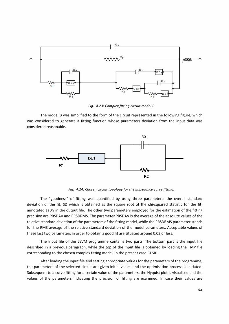
63
Fig. 4.23: Complex fitting circuit model B
The model B was simplified to the form of the circuit represented in the following figure, which
was considered to generate a fitting function whose parameters deviation from the input data was
considered reasonable.
Fig. 4.24: Chosen circuit topology for the impedance curve fitting.
The “goodness” of fitting was quantified by using three parameters: the overall standard
deviation of the fit, SD which is obtained as the square root of the chi-squared statistic for the fit,
annotated as XS in the output file. The other two parameters employed for the estimation of the fitting
precision are PRSDAV and PRSDRMS. The parameter PRSDAV is the average of the absolute values of the
relative standard deviation of the parameters of the fitting model, while the PRSDRMS parameter stands
for the RMS average of the relative standard deviation of the model parameters. Acceptable values of
these last two parameters in order to obtain a good fit are situated around 0.03 or less.
The input file of the LEVM programme contains two parts. The bottom part is the input file
described in a previous paragraph, while the top of the input file is obtained by loading the TMP file
corresponding to the chosen complex fitting model, in the present case BTMP.
After loading the input file and setting appropriate values for the parameters of the programme,
the parameters of the selected circuit are given initial values and the optimisation process is initiated.
Subsequent to a curve fitting for a certain value of the parameters, the Nyquist plot is visualised and the
values of the parameters indicating the precision of fitting are examined. In case their values are

64
considered acceptable, the fitting process is abandoned. In case their values are unsatisfactory, the
fitting process is continued by changing one or more parameters of the fitting model. At every point in
the fitting process at least one of the parameters has to be kept free, otherwise the fitting process
cannot be carried out [39].
The following figure emphasises the original impedance curve (in red) obtained from the
impedance spectroscopy measurement performed with the TrueEIS-Data impedance meter and the
corresponding fitting curve (in blue) obtained by performing the CNLS fitting with the LEVM programme
for the BYD tested cell 1. The circuit used for fitting the impedance of this cell is the one shown in Fig.
4.24. The values of the circuit parameters which yield this fitting curve are the following:
R1= 0.591 mΩ
R2=0.115 mΩ
C2=53.04 µF
RDE1=0.1 mΩ
TDE1= 5.301266 mF
PHIDE1=0.525
NDE1=3
The value of the parameter NDE1 of the distributed element DE1 is an indicator of the type of
distributed element chosen in order to implement the curve fitting. This option is available in case of
each distributed element present in the chosen complex fitting model. The chosen option number 3 for
NDE1 is means that the distributed element DE1 represents the second topology of CPE, described
previously, in which the CPE is in parallel with a resistance.
The parameters indicating the “goodness” of fitting have the following values:
Sigma Squared Estimate, XS=0.05145
Sigmaf Estimate, SD=0.2268
PDRSAV=0.025627
PDRSRMS=0.02567
Judging by the values obtained for these last four parameters, one could get to the conclusions
that the precision of the performed fitting in case of cell 1 is satisfactory.
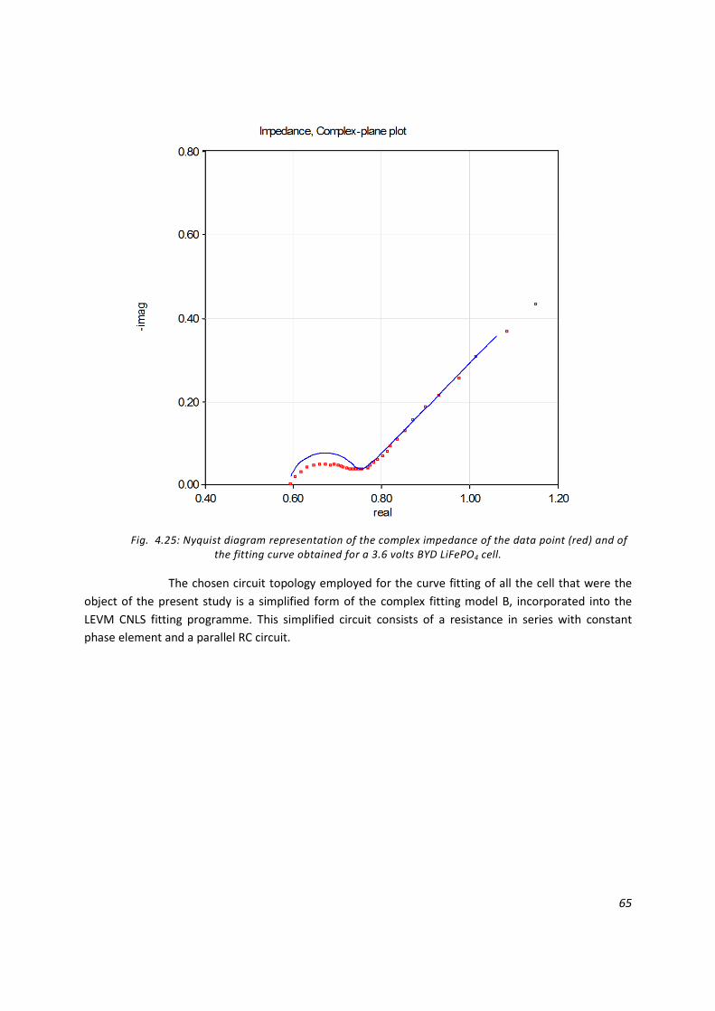
65
Fig. 4.25: Nyquist diagram representation of the complex impedance of the data point (red) and of the fitting curve obtained for a 3.6 volts BYD LiFePO4 cell.
The chosen circuit topology employed for the curve fitting of all the cell that were the
object of the present study is a simplified form of the complex fitting model B, incorporated into the
LEVM CNLS fitting programme. This simplified circuit consists of a resistance in series with constant
phase element and a parallel RC circuit.

66
67
5 Simulations and Results
The emphasis in the previous chapters of the present study was on describing the conditions
under which the testing process was performed and on building a lithium ion battery model which would
incorporate the ageing phenomena that the tested cells were facing during the testing period. The
present chapter will be oriented towards presenting the acquired experimental results and performing
the lifetime analysis of different Battery Energy Storage Systems under various stress conditions. The
basis for calculating the parameters quantifying the performance degradation of the BES are
represented by the values obtained experimentally by execution of the laboratory tests.
The first section of the chapter will be dedicated to highlighting the experimental data obtained,
followed by a description of the parameters used in developing the battery model. The last part of the
chapter will try to emphasize the effect of the ageing factors on different BES topologies, by evaluating
the values obtained for the ageing factors in each study case and determining the lifetime of the
evaluated BES topology.
5.1 Experimental Results
The experimental part of the project was divided into two periods of time: the first period was
allocated for testing a group of two LiFePO4 cells, placed in series inside the climatic chamber, at the
chamber ambient temperature of 50 °C. The second part of the laboratory tests was dedicated to testing
other two LiFePO4 cells, at the chamber ambient temperature of 40 °C. The control system of the
climatic chamber limits the temperature variations inside the chamber around the value set by the user
for the ambient chamber temperature, such that major variations of the surface temperature of the
cells compared to the ambient temperature were not observed. The temperature on the surface of the
cells was kept in a range of ±4 or maximum 5 °C around the chamber ambient temperature, larger
variations being noticed only after large periods of testing or after the cells have faced a pronounced
degradation of their performance.
The variations in the temperatures of the first two cells, cells annotated as cell 1 and cell 2 and
tested at the chamber ambient temperature of 50 °C, are emphasised in figure 5.1. The graph
represents the temperature behaviour of the two cells over a period of time consisting of several days of
testing. It is easy to notice that the cell temperature fluctuations compared to the temperature of the
chamber are smaller during the first testing days. The temperature variations will increase as the cells
will be subjected to an augmented degradation, as an effect of the application of stress factors over a
long period of time. The differences between the surface temperatures of the two cells will increase as
well, as a consequence of the different effects that the degrading factors have on the cells. These
differences in the cell surface temperatures are mainly given by their construction, making one of them,
considered the weak link, more vulnerable to degradation. The steep decrements in the cell
temperature correspond to the starting point of a new testing day.
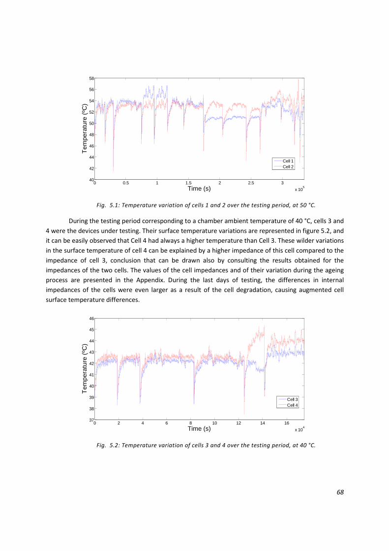
68
Fig. 5.1: Temperature variation of cells 1 and 2 over the testing period, at 50 °C.
During the testing period corresponding to a chamber ambient temperature of 40 °C, cells 3 and
4 were the devices under testing. Their surface temperature variations are represented in figure 5.2, and
it can be easily observed that Cell 4 had always a higher temperature than Cell 3. These wilder variations
in the surface temperature of cell 4 can be explained by a higher impedance of this cell compared to the
impedance of cell 3, conclusion that can be drawn also by consulting the results obtained for the
impedances of the two cells. The values of the cell impedances and of their variation during the ageing
process are presented in the Appendix. During the last days of testing, the differences in internal
impedances of the cells were even larger as a result of the cell degradation, causing augmented cell
surface temperature differences.
Fig. 5.2: Temperature variation of cells 3 and 4 over the testing period, at 40 °C.
0 0.5 1 1.5 2 2.5 3
x 105
40
42
44
46
48
50
52
54
56
58
Time (s)
Tem
pera
ture
(ºC
)
Cell 1Cell 2
0 2 4 6 8 10 12 14 16
x 104
37
38
39
40
41
42
43
44
45
46
Time (s)
Tem
pera
ture
(ºC
)
Cell 3Cell 4
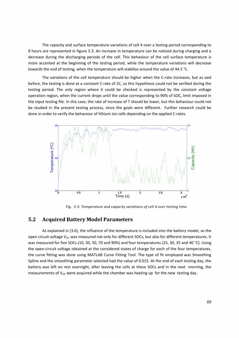
69
The capacity and surface temperature variations of cell 4 over a testing period corresponding to
8 hours are represented in figure 5.3. An increase in temperature can be noticed during charging and a
decrease during the discharging periods of the cell. This behaviour of the cell surface temperature is
more accented at the beginning of the testing period, while the temperature variations will decrease
towards the end of testing, when the temperature will stabilise around the value of 44.5 °C.
The variations of the cell temperature should be higher when the C-rate increases, but as said
before, the testing is done at a constant C-rate of 2C, so this hypothesis could not be verified during the
testing period. The only region where it could be checked is represented by the constant voltage
operation region, when the current drops until the value corresponding to 90% of SOC, limit imposed in
the input testing file. In this case, the rate of increase of T should be lower, but this behaviour could not
be studied in the present testing process, since the goals were different. Further research could be
done in order to verify the behaviour of lithium ion cells depending on the applied C-rates.
Fig. 5.3: Temperature and capacity variations of cell 4 over testing time.
5.2 Acquired Battery Model Parameters
As explained in (3.6), the influence of the temperature is included into the battery model, so the
open circuit voltage VOC was measured not only for different SOCs, but also for different temperatures. It
was measured for five SOCs (10, 30, 50, 70 and 90%) and four temperatures (25, 30, 35 and 40 °C). Using
the open-circuit voltage obtained at the considered states of charge for each of the four temperatures,
the curve fitting was done using MATLAB Curve Fitting Tool. The type of fit employed was Smoothing
Spline and the smoothing parameter selected had the value of 0.015. At the end of each testing day, the
battery was left on rest overnight, after leaving the cells at these SOCs and in the next morning, the
measurements of VOC were acquired while the chamber was heating up for the new testing day.
0 0.5 1 1.5 2 2.5 3
x 104
35
40
45
Time (s)
Tem
pera
ture
(ºC
)
0 0.5 1 1.5 2 2.5 3
x 104
0
20
40
Cap
acity
(A
h)

70
Fig. 5.4: Cell open-circuit voltage as a function of SOC, for different temperatures.
In the figure above, it can be seen that the temperature influence on the values of the open-
circuit voltage are insignificant [33]. A maximum variation of 4 mV can be observed at low SOCs,
difference between 25 to 40 °C. Therefore, it was decided not to include in the model the effect of
temperature on the VOC and some other already available data, represented in the next figure, was
utilised. The VOC data was acquired at room temperature (around 20 °C) for 11 different values of SOC.
Fig. 5.5: Open-circuit voltage as a function of SOC, at 20 °C.
The parameters of the internal impedance, which are presented in table A.1 of appendix A, were
also measured for different SOCs and temperature. Two types of battery model topologies were
simulated, one of them containing only resistances and the other topology including both resistances
and capacitances, but no difference in the voltage characteristic could be observed, so first battery
model type was chosen as model used in the simulation file. In Fig. 5.6, the total resistance of the
battery model is plotted as a function of SOC. It has a flat characteristic, meaning that it has similar
10 20 30 40 50 60 70 80 90
3.18
3.2
3.22
3.24
3.26
3.28
3.3
3.32
3.34
SOC (%)
Ope
n C
ircui
t Vol
tage
(V
)
Voc vs. SOC at 25 ºC 25 ºC fittingVoc vs. SOC at 30 ºC 30 ºC fittingVoc vs. SOC at 35 ºC 35 ºC fittingVoc vs. SOC at 40 ºC 40 ºC fitting
0 10 20 30 40 50 60 70 80 90 1002.4
2.5
2.6
2.7
2.8
2.9
3
3.1
3.2
3.3
SOC (%)
Ope
n C
ircui
t Vol
tage
(V
)
Voc vs. SOC at TambVoc fitting

71
values for different SOCs. The temperature has a major influence on the values of the battery resistance,
fact emphasised by the graph.
Fig. 5.6: Internal resistance of the cell in function of SOC for different temperatures.
As a consequence, only the temperature effect on the resistance was taken into account in the
determination of this battery parameter. The flat shape of the resistance and its variation in function of
temperature can be seen in [40].
Fig. 5.7: Internal resistance as a function of temperature.
The ageing of the cells caused by calendar life was not measured experimentally, but some data
was obtained from the manufacturer. For 20 °C, the degradation in one year of storage is 5% and for the
second and consecutive years is considered to be 3%. Having these calendar life ageing references, one
can already conclude that the maximum lifetime of this kind of batteries at 20 °C is 6 years. An
extrapolation for 30, 40 and 50 °C was done using Arrhenius Law, which says that the stress factors
increase by a factor of 2 for each increment of 10 °C. The curve fitting obtained for calendar life for the
10 20 30 40 50 60 70 80 90
0.75
0.8
0.85
0.9
0.95
SOC (%)
Res
ista
nce
(mO
hms)
R vs. SOC at 25 ºC 25 ºC fittingR vs. SOC at 35 ºC 35 ºC fittingR vs. SOC at 45 ºC 45 ºC fitting
25 30 35 40 45
0.76
0.78
0.8
0.82
0.84
0.86
0.88
0.9
0.92
0.94
0.96
Temperature (ºC)
Res
ista
nce
(mO
hms)
R vs. TR (T) fitting

72
four temperatures previously mentioned, is presented below. The increase in capacity fade with
temperature is obvious.
Fig. 5.8: Capacity fade at different temperatures, caused by calendar life ageing.
Additionally, a surface fitting equation representing the capacity fade as a function of time and
temperature was obtained, such that the increased degradation caused by calendar life to the BES as
time passes by, could be quantified. The surface plot is given in Fig. 5.9.
Fig. 5.9: Surface plot representing the capacity fade as a function of time and temperature, degradation caused by calendar life.
One of the main outcomes of the testing process performed in the present study is represented
by the capacity fade caused by the cycles applied to the cells tested under the two different climatic
chamber temperature. The cycling factor was already defined in chapter 3 as f1 and is being added to
the calendar life ageing factor f2 in order to determine the total capacity fade of the cells in a certain
period of time. In order to be able to determine a proper relation describing the capacity fade caused by
0 10 20 30 40 50 60 700
0.1
0.2
0.3
0.4
0.5
0.6
0.7
0.8
0.9
1
Time (months)
Rem
aini
ng c
apac
ity (
p.u.
)
C vs. t at 20 ºC 20 ºC fittingC vs. t at 30 ºC 30 ºC fittingC vs. t at 40 ºC 40 ºC fittingC vs. t at 50 ºC 50 ºC fitting
2025
3035
4045
50
0 10 20 30 40 50 60 70
0
0.2
0.4
0.6
0.8
1
Temperature (ºC)Time (months)
Cap
acity
(p.u
.)

73
the cycling process, three capacity tests were performed in the case of each temperature. The
degradation levels obtained after performing the last capacity measurements in each temperature case
were of 0.6 % degradation for the cells tested at 40 °C and more than 3 % for the cells tested at 50 °C.
These values would correspond to approximately 1 year and one month of applied testing signal. From
these degradation results the capacity fades corresponding to other temperatures, such as 30 or 20 °C,
can be deduced by employing Arrhenius law. The degradation obtained experimentally is shown in the
next figure with each correspondent fitting. As the figure emphasises, temperature has a major
influence in the augmentation of the capacity fade process during cycling.
Fig. 5.10: Cell capacity variation as a function of capacity throughput for different temperatures, in
case of ageing produced by cycling.
The tridimensional graph, representing the capacity fade (given in the per unit system) as a
function of capacity throughput and temperature, is presented below, where a sudden drop in capacity
can be observed between 40 °C and 50 °C. In order to be able to have several fitting options, not only
linear variation of the capacity fade as a function of capacity throughput, at least three values
representing the capacity fade at moments corresponding to different capacity throughputs needed to
be acquired. As a conclusion, the more capacity tests are performed, the better the representation of
the capacity fade process becomes. The execution of numerous capacity tests comes at the cost of the
testing time needed between two consecutive capacity tests in order to notice differences in the cell
capacity, time which summed up leads to a lengthy total testing period, unavailable in some cases.
0 1000 2000 3000 4000 5000 6000 70000.965
0.97
0.975
0.98
0.985
0.99
0.995
1
Capacity Throughput (Ah)
Rem
aini
ng C
apac
ity (
p.u.
)
C vs. Cth at 40 ºC 40 ºC fitting (experimental)C vs. Cth at 50ºC 50 ºC fitting (experimental)C vs. Cth at 30 ºC 30 ºC fitting (Arrhenius)C vs. Cth at 20 ºC 20 ºC fitting (Arrhenius)
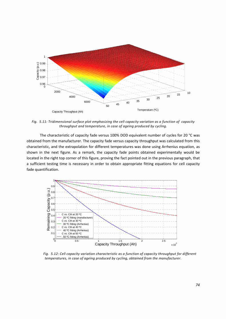
74
Fig. 5.11: Tridimensional surface plot emphasizing the cell capacity variation as a function of capacity throughput and temperature, in case of ageing produced by cycling.
The characteristic of capacity fade versus 100% DOD equivalent number of cycles for 20 °C was
obtained from the manufacturer. The capacity fade versus capacity throughput was calculated from this
characteristic, and the extrapolation for different temperatures was done using Arrhenius equation, as
shown in the next figure. As a remark, the capacity fade points obtained experimentally would be
located in the right top corner of this figure, proving the fact pointed out in the previous paragraph, that
a sufficient testing time is necessary in order to obtain appropriate fitting equations for cell capacity
fade quantification.
Fig. 5.12: Cell capacity variation characteristic as a function of capacity throughput for different temperatures, in case of ageing produced by cycling, obtained from the manufacturer.
1015
2025
303540
4550
0
2000
4000
6000
0.96
0.97
0.98
0.99
1
Temperature (ºC)Capacity Throughput (Ah)
Cap
acity
(p.
u.)
0 0.5 1 1.5 2 2.5
x 105
0
0.1
0.2
0.3
0.4
0.5
0.6
0.7
0.8
0.9
1
Capacity Throughput (Ah)
Rem
aini
ng C
apac
ity (
p.u.
)
C vs. Cth at 20 ºC 20 ºC fitting (manufacturer)C vs. Cth at 30 ºC 30 ºC fitting (Arrhenius)C vs. Cth at 40 ºC 40 ºC fitting (Arrhenius)C vs. Cth at 50 ºC 50 ºC fitting (Arrhenius)
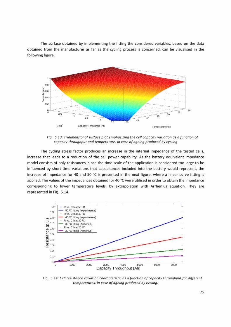
75
The surface obtained by implementing the fitting the considered variables, based on the data
obtained from the manufacturer as far as the cycling process is concerned, can be visualised in the
following figure.
Fig. 5.13: Tridimensional surface plot emphasizing the cell capacity variation as a function of capacity throughput and temperature, in case of ageing produced by cycling
The cycling stress factor produces an increase in the internal impedance of the tested cells,
increase that leads to a reduction of the cell power capability. As the battery equivalent impedance
model consists of only resistances, since the time scale of the application is considered too large to be
influenced by short time variations that capacitances included into the battery would represent, the
increase of impedance for 40 and 50 °C is presented in the next figure, where a linear curve fitting is
applied. The values of the impedances obtained for 40 °C were utilised in order to obtain the impedance
corresponding to lower temperature levels, by extrapolation with Arrhenius equation. They are
represented in Fig. 5.14.
Fig. 5.14: Cell resistance variation characteristic as a function of capacity throughput for different temperatures, in case of ageing produced by cycling.
2025
3035
4045
50
00.5
11.5
22.5
x 105
0
0.2
0.4
0.6
0.8
1
Temperature (ºC)Capacity Throughput (Ah)
Cap
acity
(p.
u.)
0 1000 2000 3000 4000 5000 6000 70001
1.1
1.2
1.3
1.4
1.5
1.6
1.7
1.8
1.9
2
Capacity Throughput (Ah)
Res
ista
nce
(p.u
.)
R vs. Cth at 50 ºC 50 ºC fitting (experimental)R vs. Cth at 40 ºC 40 ºC fitting (experimental)R vs. Cth at 30 ºC 30 ºC fitting (Arrhenius)R vs. Cth at 20 ºC 20 ºC fitting (Arrhenius)
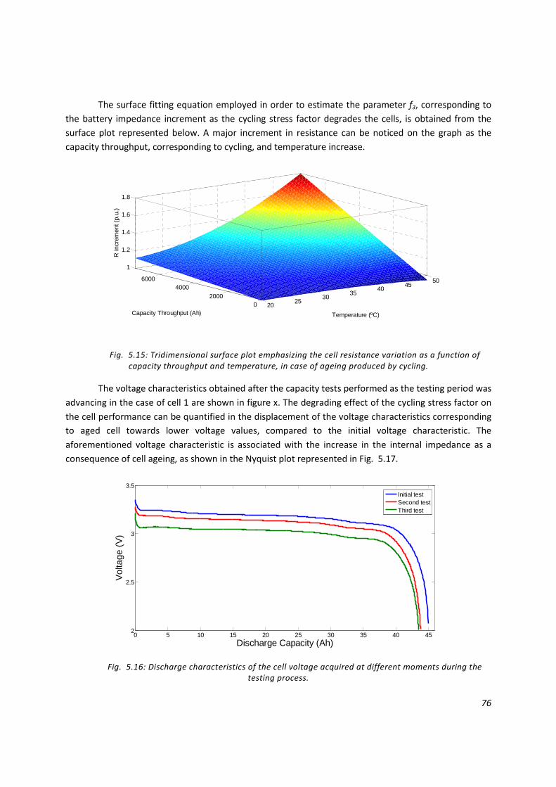
76
The surface fitting equation employed in order to estimate the parameter f3, corresponding to
the battery impedance increment as the cycling stress factor degrades the cells, is obtained from the
surface plot represented below. A major increment in resistance can be noticed on the graph as the
capacity throughput, corresponding to cycling, and temperature increase.
Fig. 5.15: Tridimensional surface plot emphasizing the cell resistance variation as a function of capacity throughput and temperature, in case of ageing produced by cycling.
The voltage characteristics obtained after the capacity tests performed as the testing period was
advancing in the case of cell 1 are shown in figure x. The degrading effect of the cycling stress factor on
the cell performance can be quantified in the displacement of the voltage characteristics corresponding
to aged cell towards lower voltage values, compared to the initial voltage characteristic. The
aforementioned voltage characteristic is associated with the increase in the internal impedance as a
consequence of cell ageing, as shown in the Nyquist plot represented in Fig. 5.17.
Fig. 5.16: Discharge characteristics of the cell voltage acquired at different moments during the testing process.
2025
3035
4045
50
02000
40006000
1
1.2
1.4
1.6
1.8
Temperature (ºC)Capacity Throughput (Ah)
R in
crem
ent (
p.u.
)
0 5 10 15 20 25 30 35 40 452
2.5
3
3.5
Discharge Capacity (Ah)
Vol
tage
(V
)
Initial testSecond testThird test
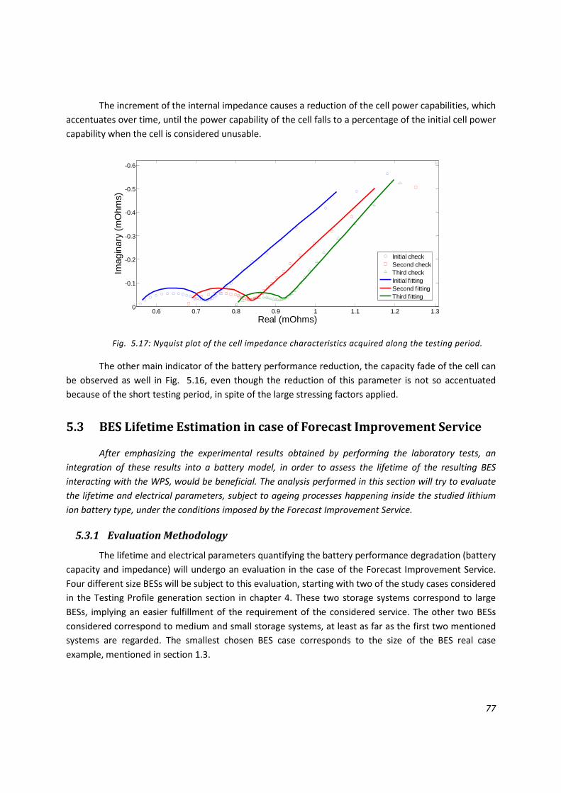
77
The increment of the internal impedance causes a reduction of the cell power capabilities, which
accentuates over time, until the power capability of the cell falls to a percentage of the initial cell power
capability when the cell is considered unusable.
Fig. 5.17: Nyquist plot of the cell impedance characteristics acquired along the testing period.
The other main indicator of the battery performance reduction, the capacity fade of the cell can
be observed as well in Fig. 5.16, even though the reduction of this parameter is not so accentuated
because of the short testing period, in spite of the large stressing factors applied.
5.3 BES Lifetime Estimation in case of Forecast Improvement Service
After emphasizing the experimental results obtained by performing the laboratory tests, an
integration of these results into a battery model, in order to assess the lifetime of the resulting BES
interacting with the WPS, would be beneficial. The analysis performed in this section will try to evaluate
the lifetime and electrical parameters, subject to ageing processes happening inside the studied lithium
ion battery type, under the conditions imposed by the Forecast Improvement Service.
5.3.1 Evaluation Methodology
The lifetime and electrical parameters quantifying the battery performance degradation (battery
capacity and impedance) will undergo an evaluation in the case of the Forecast Improvement Service.
Four different size BESs will be subject to this evaluation, starting with two of the study cases considered
in the Testing Profile generation section in chapter 4. These two storage systems correspond to large
BESs, implying an easier fulfillment of the requirement of the considered service. The other two BESs
considered correspond to medium and small storage systems, at least as far as the first two mentioned
systems are regarded. The smallest chosen BES case corresponds to the size of the BES real case
example, mentioned in section 1.3.
0.6 0.7 0.8 0.9 1 1.1 1.2 1.3
-0.6
-0.5
-0.4
-0.3
-0.2
-0.1
0
Real (mOhms)
Imag
inar
y (m
Ohm
s)
Initial checkSecond checkThird checkInitial fittingSecond fittingThird fitting
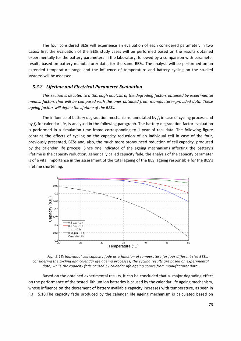
78
The four considered BESs will experience an evaluation of each considered parameter, in two
cases: first the evaluation of the BESs study cases will be performed based on the results obtained
experimentally for the battery parameters in the laboratory, followed by a comparison with parameter
results based on battery manufacturer data, for the same BESs. The analysis will be performed on an
extended temperature range and the influence of temperature and battery cycling on the studied
systems will be assessed.
5.3.2 Lifetime and Electrical Parameter Evaluation
This section is devoted to a thorough analysis of the degrading factors obtained by experimental
means, factors that will be compared with the ones obtained from manufacturer-provided data. These
ageing factors will define the lifetime of the BESs.
The influence of battery degradation mechanisms, annotated by f1 in case of cycling process and
by f2 for calendar life, is analysed in the following paragraph. The battery degradation factor evaluation
is performed in a simulation time frame corresponding to 1 year of real data. The following figure
contains the effects of cycling on the capacity reduction of an individual cell in case of the four,
previously presented, BESs and, also, the much more pronounced reduction of cell capacity, produced
by the calendar life process. Since one indicator of the ageing mechanisms affecting the battery’s
lifetime is the capacity reduction, generically called capacity fade, the analysis of the capacity parameter
is of a vital importance in the assessment of the total ageing of the BES, ageing responsible for the BES’s
lifetime shortening.
Fig. 5.18: Individual cell capacity fade as a function of temperature for four different size BESs, considering the cycling and calendar life ageing processes; the cycling results are based on experimental
data, while the capacity fade caused by calendar life ageing comes from manufacturer data.
Based on the obtained experimental results, it can be concluded that a major degrading effect
on the performance of the tested lithium ion batteries is caused by the calendar life ageing mechanism,
whose influence on the decrement of battery available capacity increases with temperature, as seen in
Fig. 5.18.The capacity fade produced by the calendar life ageing mechanism is calculated based on
20 25 30 35 40 45 500.6
0.65
0.7
0.75
0.8
0.85
0.9
0.95
1
Temperature (ºC)
Cap
acity
(p.
u.)
0.2 p.u. - 1 h0.5 p.u. - 1 h1 p.u. - 2 h0.95 p.u. - 6 hCalendar Life
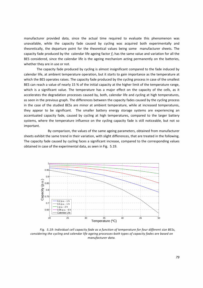
79
manufacturer provided data, since the actual time required to evaluate this phenomenon was
unavailable, while the capacity fade caused by cycling was acquired both experimentally and
theoretically, the departure point for the theoretical values being some manufacturer sheets. The
capacity fade produced by the calendar life ageing factor f2 has the same value and variation for all the
BES considered, since the calendar life is the ageing mechanism acting permanently on the batteries,
whether they are in use or not.
The capacity fade produced by cycling is almost insignificant compared to the fade induced by
calendar life, at ambient temperature operation, but it starts to gain importance as the temperature at
which the BES operates raises. The capacity fade produced by the cycling process in case of the smallest
BES can reach a value of nearly 15 % of the initial capacity at the higher limit of the temperature range,
which is a significant value. The temperature has a major effect on the capacity of the cells, as it
accelerates the degradation processes caused by, both, calendar life and cycling at high temperatures,
as seen in the previous graph. The differences between the capacity fades caused by the cycling process
in the case of the studied BESs are minor at ambient temperature, while at increased temperatures,
they appear to be significant. The smaller battery energy storage systems are experiencing an
accentuated capacity fade, caused by cycling at high temperatures, compared to the larger battery
systems, where the temperature influence on the cycling capacity fade is still noticeable, but not so
important.
By comparison, the values of the same ageing parameters, obtained from manufacturer
sheets exhibit the same trend in their variation, with slight differences, that are treated in the following.
The capacity fade caused by cycling faces a significant increase, compared to the corresponding values
obtained in case of the experimental data, as seen in Fig. 5.19.
Fig. 5.19: Individual cell capacity fade as a function of temperature for four different size BESs, considering the cycling and calendar life ageing processes-both types of capacity fades are based on
manufacturer data.
20 25 30 35 40 45 50
0.65
0.7
0.75
0.8
0.85
0.9
0.95
1
Temperature (ºC)
Cap
acity
(p.
u.)
0.2 p.u. - 1 h0.5 p.u. - 1 h1 p.u. - 2 h0.95 p.u. - 6 hCalendar Life

80
Even at the lower temperature limit, the values of the capacity fade are slightly augmented,
compared to the previous case, while, at the high temperature limit, they reach values at which some of
the studied BESs sizes, are considered to have reached their end of life. The differences between the
represented BESs are more accented as well, compared to the experimental values, emphasizing a much
higher degradation caused by cycling at high temperatures. It can be observed that the capacity fade
caused by cycling at high temperatures of small size BES is significantly larger than in the case of a large
BES, cycled at the same temperature. This difference in the capacity fades of the two storage systems is
greatly influenced by temperature increase.
The second type of fade present in rechargeable batteries, the power fade mechanism, is
determined by an increase in the internal impedance of the battery. The same ageing mechanisms
(cycling and calendar life) are responsible for the increase of battery impedance, another macroscopic
effect of ageing from an electrical point of view, besides the reduction in the capacity of the cells. In the
present study, the equivalent impedance model of the battery takes into consideration only resistances,
meaning a reduction of the battery impedance to resistances. Their variation is represented in Fig. 5.20,
as a function of temperature, for the considered BES study cases. The graphs represented in the figure
are based on the parameter values obtained by curve fitting of the impedance results measured
experimentally with the TrueEIS-Data impedance meter, fitting described in detail in section 4.4.
Fig. 5.20: Individual Lithium Iron Phosphate cell internal impedance variation with temperature, in case of four different BES sizes, based on experimentally obtained results.
The resistance variations, represented by the factor f3, were obtained from the acquired
experimental data. A temperature increase appears to produce a major augmentation of their values.
The increase in resistance is much larger for smaller storage systems, as can be seen in the above figure.
The differences between different size BESs are more pronounced at high temperatures.
The resistance results, plotted in figure 5.23, were calculated in a different manner, based on
the behavior of the battery model, caused by the reduced capacity throughput obtained from
manufacturer data, in comparison with the experimentally acquired capacity throughput. The difference
between the experimental and theoretical (based on manufacturer data) capacity throughputs resides in
20 25 30 35 40 45 501
1.5
2
2.5
3
3.5
4
4.5
5
Temperature (ºC)
Res
ista
nce
(p.u
.)
0.2 p.u. - 1 h0.5 p.u. - 1 h1 p.u. - 2 h0.95 p.u. - 6 h

81
the differences between the capacity fades of the experimental and manufacturer based data,
differences noticeable in figures 5.20 and 5.21, for each considered BES. The higher capacity fade
obtained based on manufacturer data implies less battery capacity available for use compared to the
experimental one, which means less capacity throughput than in the case of the experimental case.
As an additional remark, the errors between the forecast power and power output of the wind
power generating unit with BES included, based on manufacturer data and on experimental data,
respectively, were calculated. As the obtained capacity fade based on manufacturer data was higher,
the corresponding error was higher as well, while the obtained value for the SR was lower, meaning a
worsening of the performance of the BES with increased battery ageing.
Since no manufacturer data, representing the impedance variation over time, was available, the
equation used to obtain the resistance variation as a function of temperature in figure 5.20 was
employed in figure 5.21, as well. The difference between the capacity throughput obtained
experimentally and the one based on manufacturer sheets is the cause of the differences between the
resistances in figures 5.22 and 5.23.
Fig. 5.21: Individual Lithium Iron Phosphate cell internal impedance variation with temperature, in case of four different BES sizes, based on manufacturer-provided data.
By taking a closer look to the Fig. 5.22 emphasising the lifetime estimates of the four, different
sized BESs for a relevant temperature range from these systems operation point of view, one can easily
observe the trends regarding lifetime variation as the operating temperature of the BES is augmented.
The behaviour of all studied systems from their lifetime point of view follows the same trend.
The temperature increase has accentuated negative effects on the BES lifetime, causing a major
depletion of their estimated lifetimes.
20 25 30 35 40 45 501
1.5
2
2.5
3
3.5
4
4.5
5
Temperature (ºC)
Res
ista
nce
(p.u
.)
0.2 p.u. - 1 h0.5 p.u. - 1 h1 p.u. - 2 h0.95 p.u. - 6 h

82
Fig. 5.22: Lifetime variation as a function of temperature, for different BES, based on experimental data.
The lifetime differences between different size BES are prominent at temperatures considered
to correspond to normal operation and they tend to even off as the operation reaches temperatures
approaching the upper limit. The differences in the lifetime of the represented BES are mainly given by
the different stress levels that the cycling ageing factor exerts on them. The degradation caused by the
cycling process is more accentuated in case of smaller BES, causing a faster depletion of their
performances. The accelerated degradation suffered by these systems leads, eventually, to their faster
wear out, involving a severe reduction of their lifetime. On the other hand, in case of larger BESs, the
degrading effect of the cycling factor is diminished, mainly because of the higher charging and
discharging capabilities of the systems, which involves smaller variations in their SOCs and, accordingly,
smaller applied cycles. As known, the DOD of the applied cycles has a major influence on the lifetime of
battery systems, “deeper” cycles causing a much higher degradation than small cycles. As a
consequence, the lifetime estimates of large BESs are much larger than the lifetimes of smaller size BESs
at ambient temperature operation conditions.
As the operation temperature of the BES increases, it starts to play a more important role in the
lifetime determination of these systems, while the influence of the cycling factor on the BES lifetime is
greatly diminished. Towards the higher temperature limit, the lifetime estimates of the considered BESs
appear to be fairly homogeneous, which leads to the inference that the influence of the temperature is
predominant in the battery ageing processes at these high temperature operation limits, while the
influence of cycling is nearly nonexistent, as can be seen in the previous figure. Consequently, the
lifetime of the BESs operating at high temperatures is determined by the temperature, while the cycling
effects are minor.
The lifetime estimation results, obtained based on manufacturer data, point out the same
tendencies in the variation of the durability of the treated storage system cases, as the results acquired
from the experimental tests. The differences between the lifetimes of the four BESs are more
pronounced over the entire considered temperature range, compared to the results obtained by
20 25 30 35 40 45 500
10
20
30
40
50
60
70
Temperature (ºC)
Life
time
(mon
ths)
0.2 p.u. - 1 h0.5 p.u. - 1 h1 p.u. - 2 h0.95 p.u. - 6h
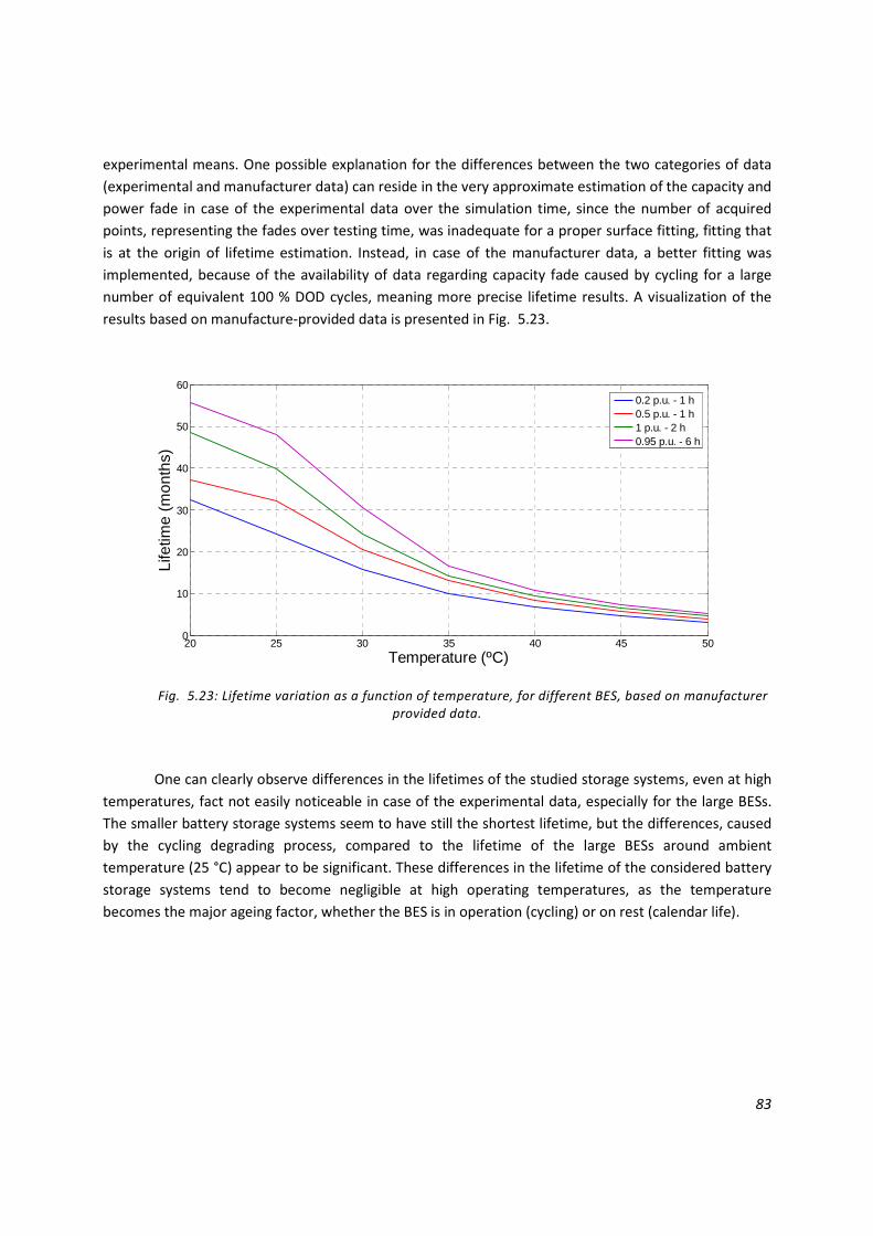
83
experimental means. One possible explanation for the differences between the two categories of data
(experimental and manufacturer data) can reside in the very approximate estimation of the capacity and
power fade in case of the experimental data over the simulation time, since the number of acquired
points, representing the fades over testing time, was inadequate for a proper surface fitting, fitting that
is at the origin of lifetime estimation. Instead, in case of the manufacturer data, a better fitting was
implemented, because of the availability of data regarding capacity fade caused by cycling for a large
number of equivalent 100 % DOD cycles, meaning more precise lifetime results. A visualization of the
results based on manufacture-provided data is presented in Fig. 5.23.
Fig. 5.23: Lifetime variation as a function of temperature, for different BES, based on manufacturer provided data.
One can clearly observe differences in the lifetimes of the studied storage systems, even at high
temperatures, fact not easily noticeable in case of the experimental data, especially for the large BESs.
The smaller battery storage systems seem to have still the shortest lifetime, but the differences, caused
by the cycling degrading process, compared to the lifetime of the large BESs around ambient
temperature (25 °C) appear to be significant. These differences in the lifetime of the considered battery
storage systems tend to become negligible at high operating temperatures, as the temperature
becomes the major ageing factor, whether the BES is in operation (cycling) or on rest (calendar life).
20 25 30 35 40 45 500
10
20
30
40
50
60
Temperature (ºC)
Life
time
(mon
ths)
0.2 p.u. - 1 h0.5 p.u. - 1 h1 p.u. - 2 h0.95 p.u. - 6 h

84
85
6 Conclusions
A future increase of wind power in the Electrical Grid points out towards the need to transform
the wind farms into reliable Wind Power Plants, capable of providing the base load covered by
conventional generation units at the moment. A major challenge regarding the augmentation of wind
power share in the Grid is represented by the unpredictability and large variations of the wind, effects
which can be mitigated to a high extent by employing ESS. Particularly, BESs present themselves as a
viable technology, capable of providing the services required by the TSO and, also, services that can
involve Energy Arbitrage, such as the Forecast Improvement Service.
The lithium ion BES technology can represent a viable solution for high power applications in
general and wind power applications, in particular, due to the good properties it has. Some of the most
important properties that recommend lithium ion batteries for high power applications are represented
by the high power and energy densities of this type of rechargeable batteries. Probably the largest
challenge as far as BES technologies in general, and LiFePO4 BES in particular are concerned, is related
to a correct estimation of their lifetime under various operating conditions (temperatures, number of
applied cycles, C-rates).These operating conditions have a major influence on their ageing processes, a
combined action of these factors making the estimation of their lifetime more difficult to achieve. A
good knowledge of ageing phenomena and of the electrical parameter variation, parameters
responsible for the quantification of battery ageing, becomes vital for a correct assessment of BES
lifetime under various operating conditions.
Setting proper conditions for the lifetime estimation of BES is a fundamental requirement for a
successful fulfillment of this goal. For a fair interpretation of the obtained experimental results, and in
order to perform an extrapolation of these results, so that the lifetime of the BES could be obtained in
an extended time period, a simulation battery model is required. The value of a developed model
resides also in the possibility to determine the lifetimes of different BESs, operating under various stress
conditions. This battery model is required to include the battery degradation processes, causing a
reduction of the battery performance in time.
In order to obtain reliable experimental results, the testing conditions and procedure have to be
clear, otherwise wrongful conditions can lead to an erroneous estimation of the electrical parameters
responsible with cell ageing leading, eventually, to misleading lifetime estimates.
The experimental results obtained in the laboratory constituted the departure point for the BES
lifetime analysis and estimation in case of four different sizes of BESs. The result interpretations point
towards a worsening of the ageing measuring parameters by applying the stress factors over long time
periods. The cycling stressing factor plays the main role around ambient temperature values, and it
affects to a much larger extent smaller size BESs, as a result of the larger cycles they have to face as a
consequence of their reduced electrical parameters (storage power and energy). The influence of cycling
on large BESs is considerably reduced compared to small BES, so their ageing is drastically diminished,
fact that points towards a much higher lifetime of these storage systems. As the operation temperature
increases, the lifetime of the BESs is severely diminished, reaching to very low values at the high limit of

86
the temperature range, compared to the values obtained at ambient temperature. On the other hand,
the lifetime estimates obtained at high temperatures are extremely homogeneous, independent of the
BES size, fact that leads to the conclusion of a decrement to a large extent of the cycling influence on the
ageing of the BES at high temperatures and massive increase of the role of temperature on the
degradation of the battery performance. This can explain the homogenization of the estimated lifetime
of small and large BES around very similar values, since the cycling stress factor is the main cause of the
lifetime estimate differences between different size BESs, around ambient temperature operation.
In order to produce a proper improvement of the wind power forecast, a huge BES
would be needed. The investments related to setting up such a large storage system might turn out to
be exaggerated. But as electrical vehicle applications start to gain in popularity, the prospects of
obtaining such an immense BES are closer to being implemented. The electrical vehicles can become a
reliable source of power, capable of fulfilling Electrical Grid services.
6.1 Future Work
During the progress of the project, it was found that several things were disregarded, while the
implementation of others was not possible, or it was outside the goals of the performed work.
One first improvement of the present work refers to the possibility to perform the ageing tests
on the cells without interruptions, in order to cause a more accentuated ageing of the cells.
Another condition in order to obtain more reliable experimental results would be represented
by testing performed on a larger range of temperatures and on a longer period of time, so that the need
to extrapolate the results by employing the Arrhenius equation would be avoided.
Implementation of calendar life ageing can be extremely beneficial, in order to obtain the
capacity fade and impedance increase of the studied types of cells, subject to calendar life ageing. By
implementing this requirement, a radical improvement of the lifetime estimation of different BESs can
be attained, by obtaining more precise parameters describing the battery model and the
transformations it undergoes along the ageing process.
By performing ageing tests at different C-rates, at the considered temperatures, the influence of
the current rates on the battery performance could be assessed and included into the battery model.
Some additional details are presented in the appendix B, so that future testing experiments
could be improved.
87
REFERENCES
1]
Pachauri, R.K., and Reisinger. (accessed 2011, April) “Climate Change 2007: Synthesis
Report: Contribution of Working Groups I, II and III to the Fourth Assessment Report of the
Intergovernmental Panel on Climate Change”. [Online].
http://www.ipcc.ch/publications_and_data/publications_ipcc_fourth_assessment_report_synthesis
_report.htm
2]
REN21, "Renewables 2010: Global Status Report," Paris, July 2010.
3]
B. Brook. (accessed 2011, April) Fukushima Nuclear Accident – a simple and accurate
explanation. [Online]. http://bravenewclimate.com/2011/03/13/fukushima-simple-explanation/
4]
(accessed 2011, April) Solar Energy Pros and Cons: Advantages and Disadvantages of Solar
Power. [Online]. http://www.solarpowerathome.com/solar-energy-pros-and-cons.html
5]
[Online]. http://www.gwec.net/index.php?id=13&L=0
6]
EWEA. (accessed 2011, April) Large scale integration of wind energy in the European Power
Supply, December 2005. [Online].
http://www.windenergie.de/fileadmin/dokumente/EWEA_Grid_report_europe.pdf
7]
C. N. Rasmussen, Improving wind power quality with energy storage.: Proceedings of the
IEEE-PES/IAS Conference on Sustainable alternative energy, 2009.
8]
B. Yang et al., On the Use of Energy Storage Technologies for Regulation Services in Electric
Power Systems with Significant Penetration of Wind Energy.: IEEE Transactions, 2008.
9]
D. Connolly, An investigation into the energy storage technologies available, for the
integration of alternative generation techniques.: University of Limerick, 2007.
10]
http://www.grist.org/wind-power/2011-04-15-no-trees-big-battery-texas-to-install-worlds-
largest-wind.
11]
(accessed April 2011) The high-power lithium-ion. [Online].
http://batteryuniversity.com/learn/article/the_high_power_lithium_ion
12]
(accessed April 2011) Rechargeable Lithium Batteries. [Online].
http://www.mpoweruk.com/lithiumS.htm

88
13]
Jim McDowall, UNDERSTANDING LITHIUM-ION TECHNOLOGY.: Saft America Inc.
14]
Altairnano Company. (accessed April 2011) Altairnano Corporate Brochure. [Online].
http://b2icontent.irpass.cc/546%2F93807.pdf?AWSAccessKeyId=1Y51NDPSZK99KT3F8VG2
15]
A. Chih-Chiang Hua and B. Zong-Wei Syue, Charge and Discharge Characteristics of Lead-
Acid Battery and LiFePO4 Battery.: The 2010 International Power Electronics Conference.
16]
Edward James William II et al., A Comparative Study of Lithium Poly-Carbon Monoflouride
(Li/CFx) and Lithium Iron Phosphate (LiFeP04) Battery Chemistries for State of Charge Indicator
Design.: IEEE International Symposium on Industrial Electronics, 2009.
17]
Hai-Ming Xie, Rong-Shun Wang, Jie-Rong Ying, Ling-Yun Zhang, and Abraham F. Jalbout,
Optimized LiFePO4–Polyacene Cathode Material for Lithium-Ion Batteries.: WILEY-VCH Verlag
GmbH & Co. KGaA, Weinheim, 2006.
18]
T. Župa and O. Líška, Charging module for newest types of rechargeable batteries LiFePO4.:
8th IEEE International Symposium on Applied Machine Intelligence and Informatics, 2010.
19]
L. Gangtie et al., An investigation of the electrochemical performance of polyaniline coated
LiFePO4 materials, Wiley InterScience, Ed.: Polymers for Advanced Technologies, vol.20, pag. 576-
580, 2009.
20]
Michel Broussely, Aging Mechanisms and Calendar-Life Predictions in Lithium-Ion Batteries.:
Advances in Lithium-Ion Batteries.
21]
M. Broussely et al., Main aging mechanisms in Li ion batteries.: Journal of Power Sources 146
(2005) 90–96.
22]
Ira Blooma et al., Effect of cathode composition on capacity fade, impedance rise and
power fade in high-power, lithium-ion cells.: Journal of Power Sources 124 (2003) 538–550.
23]
J. Vetter et al., Ageing mechanisms in lithium-ion batteries.: Journal of Power Sources 147
(2005) 269–281.
24]
H. Bindner et al., Lifetime Modelling of Lead Acid Batteries, 8755034411th ed. Denmark:
Risø National Laboratory, Roskilde, 2005.
25]
Richard L. Hartmann II, AN AGING MODEL FOR LITHIUM-ION CELLS.: The Graduate Faculty
of The University of Akron, 2008.
H. Haskins et al., Battery Technology Life Verification Test Manual. Idaho Falls: Advanced

89
26] Technology Program for lithium-Ion Batteries, Idaho National Laboratory, 2005.
27]
G. Giebel, The State-of-the-Art in Short-Term Prediction of Wind Power.: Project ANEMOS,
2003.
28]
H. Madsen, A Protocol for Standardizing the Performance Evaluation Of Short-Term Wind
Power Prediction Models.: Project ANEMOS, 2004.
29]
G. Giebel, Forecast error of aggregated wind power.: Project ANEMOS, 2007.
30]
C. Amzallag, J.P. Gerey, J.L. Robert, and J. Bahuaudl, Standardization of the rainflow
counting method for fatigue analysis.: Butterworth-Heinemann Ltd, 1994.
31]
O. Erdinc, B. Vural, and M. Uzunoglu, A dynamic lithium-ion battery model considering the
effects of temperature and capacity fading.: International Conference on Clean Electrical Power,
2009.
32]
M. Chen and G. A. Rincon-Mora, Accurate Electrical Battery Model Capable of Predicting
Runtime and I-V Performance.: IEEE Transactions on Energy Conversion, Vol. 21, No. 2, June 2006.
33]
Valerie H. Johnson, Ahmad A. Pesaran, and Thomas Sack, Temperature-Dependent Battery
Models for High-Power Lithium-Ion Batteries.: 17th Electric Vehicle Symposium.
34]
P. Ramadass, Bala Haran, Ralph White, and Branko N. Popov, Mathematical modeling of the
capacity fade of Li-ion cells.: Journal of Power Sources 123 (2003) 230–240.
35]
Nick Picciano, Battery Aging and Characterization of Nickel Metal Hydride and Lead Acid
Batteries.: The Ohio State University, 2007.
36]
M. Swierczynski, Lab hardware description.
37]
O.S. Bohlen, Impedance Based Battery Monitoring.: doctorDissertation as presented to The
Institute for Power Electronics and Electrical Drives, Aachen University, 2008.
38]
FuelCon Company, TrueData-EIS – Impedance spectrum analyzer for fuell cell research and
diagnostics.: Operation manual, Version BZH005_01_33, 06/2008.
39]
J. R. Macdonald, CNLS (Complex Nonlinear Least Squares Fitting) Immittance, Inversion and
Simulation Fitting Programs for WINDOWS and MS-DOS:LEVM/LEVMW Manual.: Version8.10, 2010.
Wang Jiayuan, Sun Zechang, and Wei Xuezhe, Performance and Characteristic Research in

90
40] LiFePO4 Battery for Electric Vehicle Applications.: 978-1-4244-2601-0/09/$25.00 ©2009 IEEE.
41]
R. L. Hartmann II, AN AGING MODEL FOR LITHIUM-ION CELLS.: Akron University, 2008.

91
APPENDIX
A. Impedance parameters
The impedance parameters were measured for different SOC and temperatures. Rs and R2 were
the two parameters taken into account for the BES model. The influence of the capacitances C2 and CD1
turned out not to have any influence on the behavior of the battery model included into the Simulink
model because of the large time scale used (1 minute), so they were not included in the battery model.
The resistance of the constant phase element, RDE1 turned out to be able to take values in a large range
(of the 10 3 order) without causing any change in the CNLS fitting process, probably because of the way
the LEVM performs the fitting, requiring always a parameter that has to be free to vary, in order for the
fitting process to complete. Because of the large variations of RDE1, without any effect on the fitting
precision, it was decided that the values obtained for it were not conclusive, so it was as well neglected
in the equivalent battery model. The values obtained for the parameters are shown in the following
table.
Table A.1: Impedance parameters in function of SOC and temperature
25 °C
SOC Rs R2 C2 RDE1 CDE1
10% 0,775 0,19 0,0298 2 38,581
20% 0,776 0,197 0,0318 2 56,397
30% 0,776 0,185 0,0328 3 52,726
40% 0,779 0,17 0,0328 3 57,679
50% 0,78 0,167 0,0338 4 52,134
60% 0,781 0,17 0,0348 4 51,627
70% 0,782 0,1673 0,0348 5 44,001
80% 0,78 0,1683 0,03498 5 33,589
90% 0,779 0,1646 0,03518 6 36,544
35 °C
SOC Rs R2 C2 RDE1 CDE1
10% 0,771 0,049 0,1393 2 47,799
20% 0,766 0,0496 0,1703 3 75,917
30% 0,766 0,0456 0,1803 4 81,422
40% 0,763 0,0475 0,2403 4,5 71,66
50% 0,765 0,0443 0,2903 4,7 71,521
60% 0,765 0,0432 0,2738 4,9 57,923
70% 0,765 0,041 0,2738 5,07 56,087
80% 0,764 0,038 0,2838 5,3 63,83
90% 0,766 0,038 0,2938 5,34 71,34
45 °C
SOC Rs R2 C2 RDE1 CDE1
10% 0,712 0,0528 0,0178 0,0033 2,63

92
20% 0,75 0,00828 0,43 0,013 5,128
30% 0,75 0,00678 0,45 0,013 5,714
40% 0,75 0,00618 0,45 0,013 6,05
50% 0,747 0,0026 0,45 0,01 5,385
60% 0,747 0,0025 0,49 0,01 5,524
70% 0,746 0,00245 0,59 0,01 5,914
80% 0,7455 0,00295 0,6 0,01 7,172
90% 0,7455 0,003 0,61 0,01 7,711
Ageing parameters
During the testing process, several capacity and impedance tests were performed, in order to
assess the level of degradation caused to the cells at the two different applied temperatures. The
capacity fade and the impedance increment measurements which were used for the ageing model are
the ones highlighted in grey in Table A.2. Apparently, some mistakes were committed in some of the
tests, so one of them had to be discarded for 50 °C. It is not the case for 40 °C, where only three tests
were done, so none of them could be discarded, thus, some arrangements were needed in order to then
have logical results.
Table A.2: Capacity and impedance parameter measurements for ageing estimation
Temperature Cell nº Measurement Cell Capacity Rs R2 C2 RDE1 CDE1
50 °C
Cell 1
Initial 45,01 0,590 0,145 0,053 0,100 6,235
Second 43,78 1,490 0,115 0,061 1,850 56,215
Third 43,80 1,930 0,123 0,061 1,930 43,613
Fourth 43,54 - - - - -
Cell 2
Initial 45,17 0,650 0,215 0,030 0,900 21,923
Second 43,61 3,210 0,118 0,045 1,890 63,291
Third 43,46 0,870 0,098 0,051 4,890 110,732
Fourth 42,44 1,335 0,149 0,090 5,890 71,420
40 °C
Cell 3
Initial 43,70 0,440 0,120 0,042 2,000 69,031
Second 43,52 0,595 0,140 0,047 2,100 56,474
Third 43,77 0,596 0,129 0,057 2,100 142,330
Cell 4
First 43,86 0,560 0,152 0,030 2,000 57,929
Second 44,75 0,680 0,151 0,036 2,000 53,202
Third 43,58 0,802 0,109 0,188 2,000 44,497
The ageing factors used in the model, which are shown in Table A.3, were calculated from the
parameters presented above. The total testing time for 50 °C was 92.6 hours, while for 40 °C was 75.5
hours. This difference in testing time is not only caused by the larger capacity throughput applied in the
case of 50 °C, but also because of the problem of the delay in the acquisition data that was not taken
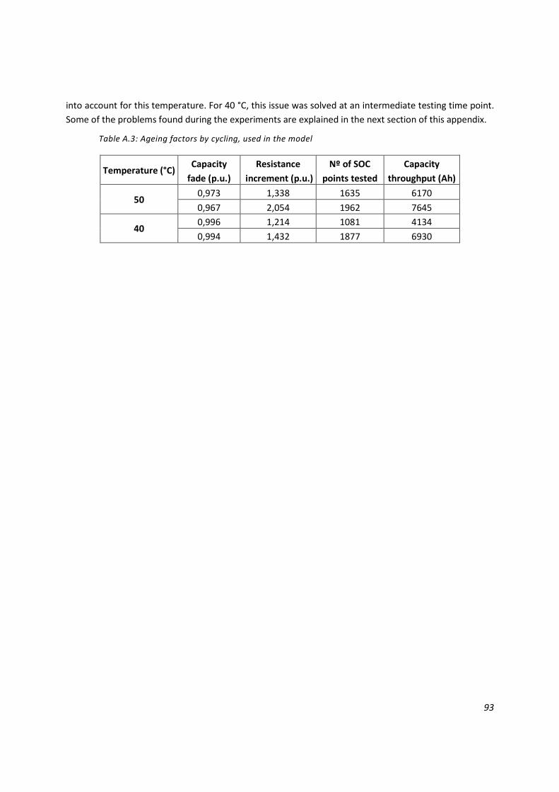
93
into account for this temperature. For 40 °C, this issue was solved at an intermediate testing time point.
Some of the problems found during the experiments are explained in the next section of this appendix.
Table A.3: Ageing factors by cycling, used in the model
Temperature (°C) Capacity Resistance Nº of SOC Capacity
fade (p.u.) increment (p.u.) points tested throughput (Ah)
50 0,973 1,338 1635 6170
0,967 2,054 1962 7645
40 0,996 1,214 1081 4134
0,994 1,432 1877 6930

94
B. Improvements for future experiments
In this section, a list of observations and problems, which were found during the experiments,
are stated, so that they can be considered for further work:
• Taking into account the delay in the data acquisition, which is explained in section 4.2, so
that the capacity acquired or delivered over time is properly calculated and as a
consequence, also the SOC. This problem was the main cause of the setup disconnections,
although at the beginning, the scaling issue was thought to be the main responsible factor
• Ensuring the fact that capacity tests are done always in the same conditions. For instance,
the cells must be discharged from/to the same level of voltage and the C-rate and the cell
temperature must be always the same, 1C and 25 °C respectively.
• Using the best quality transducer possible, so that accurate measurements of capacity are
achieved and less risk of setup disconnections is run, being able to test continuously for
large periods of time.
• Testing a minimum of 3 cells in series. This would make possible avoiding the DC Loads
limitation explained in section 4.2, meaning a discharge of the cells to their minimum
voltage level of 2 V. Besides, the constant voltage operation would start in a higher SOC.
Avoiding this operation could be very important if the effect of different C-rates in the
ageing is desired to be accounted, as well as for keeping the speed of the degradation
process.
• Shortening of the current cables as much as possible, so the constant voltage operation
would start later.
• Ensuring the fact that all the cables and plates are tightly connected to the terminals of the
cells. This experienced problem is explained after this list of improvements.
• Avoiding the use of the PC which is in charge of controlling the climatic chamber
temperature. Otherwise, its control is lost and the temperature rises indefinitely. Even not
doing that, its control is lost anyway, so further research must be done in order to find out
the cause of this loss of temperature control.
• A protection circuit (i.e. voltage comparator) could be implemented in order to prevent the
cells from discharging through the power supply, so that the safety of the setup would not
only rely on the LabView software.
After completion of the first simulation year, meaning reaching to the end of the SOC input file,
the setup experienced several disconnections during one testing day. The reason could be a decrease in
the cell capacity for increased temperatures, as specified in the manufacturer datasheet. In order to
verify this assumption, a capacity test at 50 °C and 1C was performed for both Cell 1 and Cell 2, so that,
apart from checking the reason of the disconnections, the capacity in function of temperature could be
introduced into the model. It was done after the third capacity test, when the value of the capacity has
dropped below 44 Ah. As can be seen in the next figure, the capacity obtained was of almost 44 Ah, so
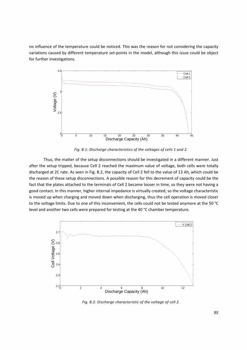
95
no influence of the temperature could be noticed. This was the reason for not considering the capacity
variations caused by different temperature set-points in the model, although this issue could be object
for further investigations.
Fig. B.1: Discharge characteristics of the voltages of cells 1 and 2.
Thus, the matter of the setup disconnections should be investigated in a different manner. Just
after the setup tripped, because Cell 2 reached the maximum value of voltage, both cells were totally
discharged at 2C rate. As seen in Fig. B.2, the capacity of Cell 2 fell to the value of 13 Ah, which could be
the reason of these setup disconnections. A possible reason for this decrement of capacity could be the
fact that the plates attached to the terminals of Cell 2 became looser in time, so they were not having a
good contact. In this manner, higher internal impedance is virtually created, so the voltage characteristic
is moved up when charging and moved down when discharging, thus the cell operation is moved closer
to the voltage limits. Due to one of this inconvenient, the cells could not be tested anymore at the 50 °C
level and another two cells were prepared for testing at the 40 °C chamber temperature.
Fig. B.2: Discharge characteristic of the voltage of cell 2.
0 5 10 15 20 25 30 35 40 452
2.5
3
3.5
Discharge Capacity (Ah)
Vol
tage
(V
)
Cell 1Cell 2
0 2 4 6 8 10 122.2
2.3
2.4
2.5
2.6
2.7
Discharge Capacity (Ah)
Cel
l Vol
tage
(V
)
V Cell 2
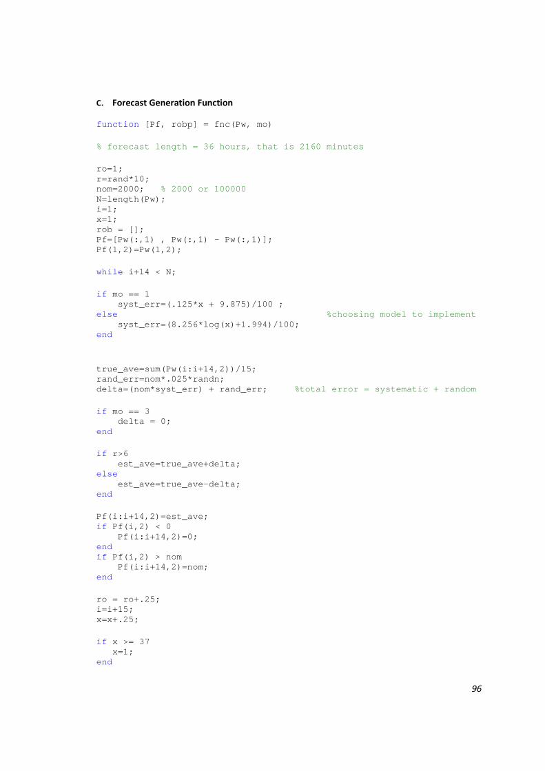
96
C. Forecast Generation Function
function [Pf, robp] = fnc(Pw, mo) % forecast length = 36 hours, that is 2160 minutes ro=1; r=rand*10; nom=2000; % 2000 or 100000 N=length(Pw); i=1; x=1; rob = []; Pf=[Pw(:,1) , Pw(:,1) - Pw(:,1)]; Pf(1,2)=Pw(1,2); while i+14 < N; if mo == 1 syst_err=(.125*x + 9.875)/100 ; else %choosing model to implement syst_err=(8.256*log(x)+1.994)/100; end true_ave=sum(Pw(i:i+14,2))/15; rand_err=nom*.025*randn; delta=(nom*syst_err) + rand_err; %total error = systematic + random if mo == 3 delta = 0; end if r>6 est_ave=true_ave+delta; else est_ave=true_ave-delta; end Pf(i:i+14,2)=est_ave; if Pf(i,2) < 0 Pf(i:i+14,2)=0; end if Pf(i,2) > nom Pf(i:i+14,2)=nom; end ro = ro+.25; i=i+15; x=x+.25; if x >= 37 x=1; end
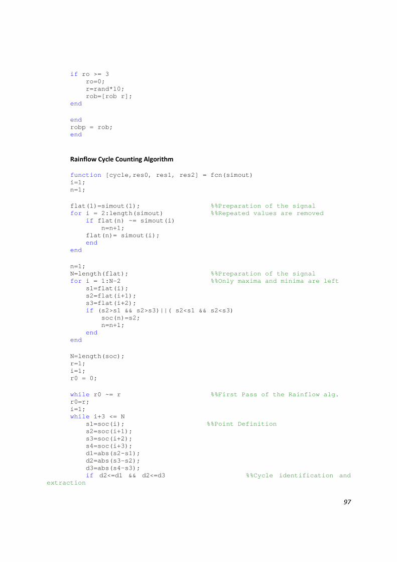
97
if ro >= 3 ro=0; r=rand*10; rob=[rob r]; end end robp = rob; end
Rainflow Cycle Counting Algorithm
function [cycle,res0, res1, res2] = fcn(simout) i=1; n=1; flat(1)=simout(1); %%Preparation of the signal for i = 2:length(simout) %%Repeated values are removed if flat(n) ~= simout(i) n=n+1; flat(n)= simout(i); end end n=1; N=length(flat); %%Preparation of the signal for i = 1:N-2 %%Only maxima and minima are left s1=flat(i); s2=flat(i+1); s3=flat(i+2); if (s2>s1 && s2>s3)||( s2<s1 && s2<s3) soc(n)=s2; n=n+1; end end N=length(soc); r=1; i=1; r0 = 0; while r0 ~= r %%First Pass of the Rainflow alg. r0=r; i=1; while i+3 <= N s1=soc(i); %%Point Definition s2=soc(i+1); s3=soc(i+2); s4=soc(i+3); d1=abs(s2-s1); d2=abs(s3-s2); d3=abs(s4-s3); if d2<=d1 && d2<=d3 %%Cycle identification and
extraction

98
cycle(r)=d2; soc(i+1)=[]; soc(i+1)=[]; N=length(soc); r=r+1; else i=i+1; end end end N = length(soc); %%Appending residue to itself a = soc(N) - soc(N-1) ; b = soc(2) - soc(1); res1=soc; if a > 0 && b < 0 %%checking for correct connection of
residue rol=1; if soc(N) > soc(1) soc(1)= []; else soc(N)= []; end end if a > 0 && b > 0 rol=2; if soc(N) < soc(1) soc(N) = []; soc(1) = []; end end if a < 0 && b < 0 rol=3; if soc(1) < soc(N) soc(N) = []; soc(1) = []; end end if a < 0 && b > 0 rol=4; if soc(N) > soc(1) soc(N) = []; else soc(1) = []; end end res0 = soc; soc = [soc soc]; N=length(soc);
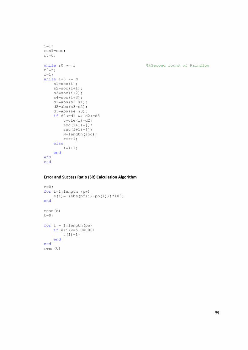
99
i=1; res1=soc; r0=0; while r0 ~= r %%Second round of Rainflow r0=r; i=1; while i+3 <= N s1=soc(i); s2=soc(i+1); s3=soc(i+2); s4=soc(i+3); d1=abs(s2-s1); d2=abs(s3-s2); d3=abs(s4-s3); if d2<=d1 && d2<=d3 cycle(r)=d2; soc(i+1)=[]; soc(i+1)=[]; N=length(soc); r=r+1; else i=i+1; end end end
Error and Success Ratio (SR) Calculation Algorithm
e=0; for i=1:length (pw) e(i)= (abs(pf(i)-po(i)))*100; end mean(e) t=0; for i = 1:length(pw) if e(i)<=5.000001 t(i)=1; end end mean(t)

100
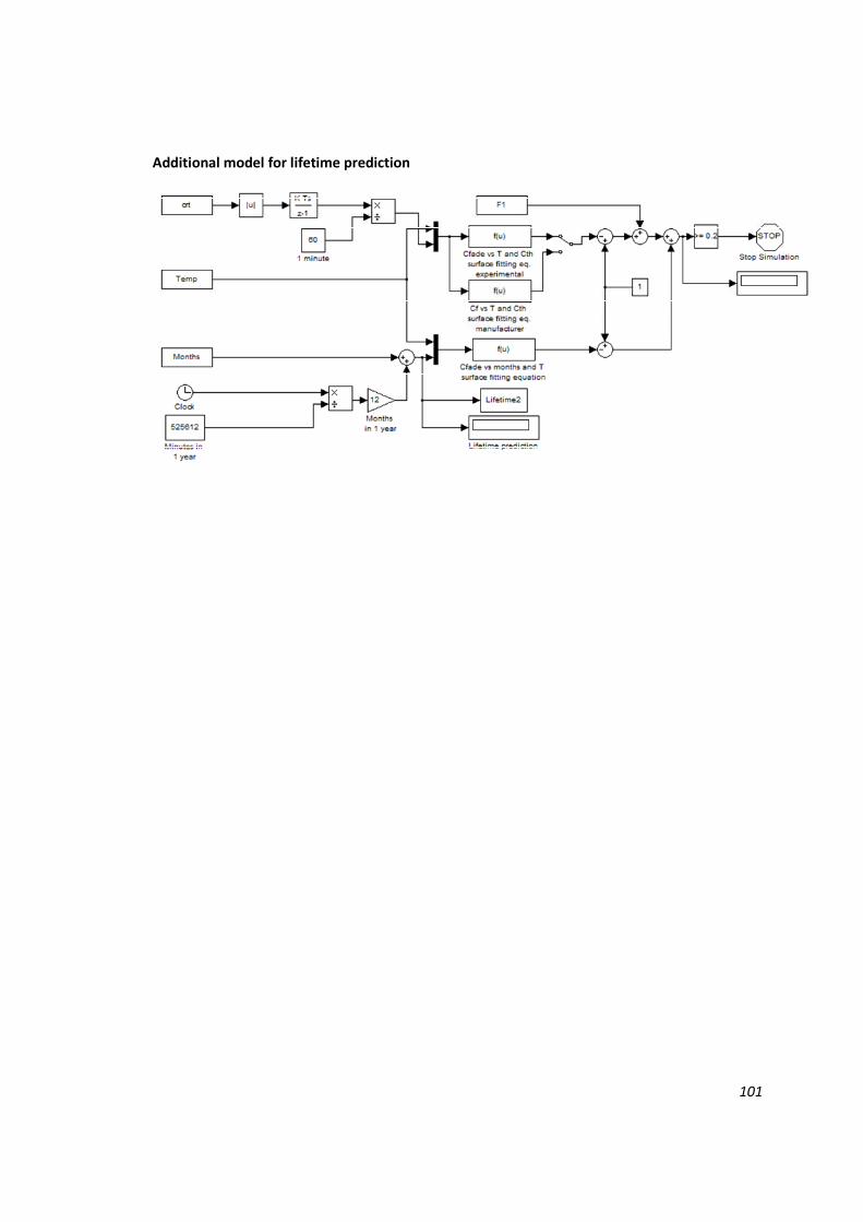
101
Additional model for lifetime prediction
Recommended