ABSTRACT
Title of dissertation: OPTIMIZATION AND EVALUATIONOF SERVICE SPEED AND RELIABILITYIN MODERN CACHING APPLICATIONS
Omri Bahat, Doctor of Philosophy, 2006
Dissertation directed by: Professor Armand M. MakowskiDepartment of Electrical and Computer Engineeringand the Institute for Systems Research
The performance of caching systems in general, and Internet caches in particular,
is evaluated by means of the user-perceived service speed, reliability of downloaded
content, and system scalability. In this dissertation, we focus on optimizing the speed
of service, as well as on evaluating the reliability and quality of data sent to users.
In order to optimize the service speed, we seek optimal replacement policies in
the first part of the dissertation, as it is well known that download delays are a direct
product of document availability at the cache; in demand-driven caches, the cache
content is completely determined by the cache replacement policy. In the literature,
many ad-hoc policies that utilize document sizes, retrieval latency, probability of
references, and temporal locality of requests, have been proposed. However, the
problem of finding optimal policies under these factors has not been pursued in any

systematic manner. Here, we take a step in that direction: Still under the Independent
Reference Model, we show that a simple Markov stationary policy minimizes the
long-run average metric induced by non-uniform documents under optional cache
replacement. We then use this result to propose a framework for operating caches
under multiple performance metrics, by solving a constrained caching problem with
a single constraint.
The second part of the dissertation is devoted to studying data reliability and
cache consistency issues: A cache object is termed consistent if it is identical to
the master document at the origin server, at the time it is served to users. Cached
objects become stale after the master is modified, and stale copies remain served to
users until the cache is refreshed, subject to network transmit delays. However, the
performance of Internet consistency algorithms is evaluated through the cache hit
rate and network traffic load that do not inform on data staleness. To remedy this,
we formalize a framework and the novel hit* rate measure, which captures consistent
downloads from the cache. To demonstrate this new methodology, we calculate the
hit and hit* rates produced by two TTL algorithms, under zero and non-zero delays,
and evaluate the hit and hit* rates in applications.

OPTIMIZATION AND EVALUATIONOF SERVICE SPEED AND RELIABILITYIN MODERN CACHING APPLICATIONS
by
Omri Bahat
Dissertation submitted to the Faculty of the Graduate School of theUniversity of Maryland, College Park in partial fulfillment
of the requirements for the degree ofDoctor of Philosophy
2006
Advisory Committee:
Professor Armand M. Makowski, ChairProfessor John S. BarasProfessor Richard J. LaProfessor Bruce JacobProfessor Eric V. Slud

c�
Copyright by
Omri Bahat
2006

DEDICATION
To Orit
ii

Contents
1 Introduction 1
1.1 Web caching . . . . . . . . . . . . . . . . . . . . . . . . . . . . . . 1
1.2 Quality of service (QoS) . . . . . . . . . . . . . . . . . . . . . . . 2
1.3 Speed of service . . . . . . . . . . . . . . . . . . . . . . . . . . . . 3
1.4 Reliability and quality of data . . . . . . . . . . . . . . . . . . . . . 4
I Finding Optimal Replacement Policies to Improve the Speed of Service 7
2 Cache Replacement Policies 9
2.1 Conventional replacement algorithms . . . . . . . . . . . . . . . . 9
2.2 Conventional versus Web caching . . . . . . . . . . . . . . . . . . 10
2.3 Replacement policies on the Web . . . . . . . . . . . . . . . . . . . 11
2.4 Finding good replacement policies . . . . . . . . . . . . . . . . . . 13
3 The Cache Model 15
3.1 The system model . . . . . . . . . . . . . . . . . . . . . . . . . . . 15
3.1.1 User requests . . . . . . . . . . . . . . . . . . . . . . . . . 15
3.1.2 The reference model . . . . . . . . . . . . . . . . . . . . . 16
3.1.3 Dynamics of the cache content . . . . . . . . . . . . . . . . 17
iii

3.2 Cache states and replacement policies . . . . . . . . . . . . . . . . 19
3.3 The probability measure . . . . . . . . . . . . . . . . . . . . . . . 21
3.4 Optimal replacement policies . . . . . . . . . . . . . . . . . . . . . 22
3.5 The cost functionals . . . . . . . . . . . . . . . . . . . . . . . . . . 24
4 A Class of Optimal Replacement Policies 27
4.1 The Dynamic Program . . . . . . . . . . . . . . . . . . . . . . . . 27
4.2 The optimal policy ���� . . . . . . . . . . . . . . . . . . . . . . . . 29
4.3 The optimal cost . . . . . . . . . . . . . . . . . . . . . . . . . . . 30
4.4 Implementing ���� . . . . . . . . . . . . . . . . . . . . . . . . . . . 33
4.5 The non-optimality of � � . . . . . . . . . . . . . . . . . . . . . . . 35
4.6 The impact of using � � instead of ���� . . . . . . . . . . . . . . . . 36
4.7 On the optimal policy with Markov requests . . . . . . . . . . . . . 39
5 Optimal Caching Under a Constraint 41
5.1 Problem formulation . . . . . . . . . . . . . . . . . . . . . . . . . 41
5.2 A Lagrangian approach . . . . . . . . . . . . . . . . . . . . . . . . 43
5.3 On the way to finding the optimal policy . . . . . . . . . . . . . . . 44
5.4 The constrained optimal replacement policy . . . . . . . . . . . . . 49
II Modeling and Measuring Internet Cache Consistency and Quality of
Data 55
6 Internet Cache Consistency 57
6.1 The cache consistency problem . . . . . . . . . . . . . . . . . . . . 57
6.2 Consistency algorithms on the Web . . . . . . . . . . . . . . . . . . 58
6.2.1 TTL algorithms . . . . . . . . . . . . . . . . . . . . . . . . 59
iv

6.2.2 Client polling . . . . . . . . . . . . . . . . . . . . . . . . . 60
6.2.3 Server invalidation . . . . . . . . . . . . . . . . . . . . . . 61
6.3 Weak vs. strong consistency models . . . . . . . . . . . . . . . . . 61
6.4 Quantifying cache consistency and QoD . . . . . . . . . . . . . . . 63
7 A Framework for Measuring Cache Consistency 65
7.1 The system model . . . . . . . . . . . . . . . . . . . . . . . . . . . 65
7.1.1 Modeling requests . . . . . . . . . . . . . . . . . . . . . . 66
7.1.2 Modeling document updates . . . . . . . . . . . . . . . . . 67
7.2 Basic assumptions . . . . . . . . . . . . . . . . . . . . . . . . . . . 67
7.3 Hit rates and QoD . . . . . . . . . . . . . . . . . . . . . . . . . . . 68
7.4 Requests and updates in applications . . . . . . . . . . . . . . . . . 69
7.5 Bounds on the renewal function . . . . . . . . . . . . . . . . . . . 70
7.5.1 Distribution-free bounds . . . . . . . . . . . . . . . . . . . 70
7.5.2 NBUE and NWUE distributions . . . . . . . . . . . . . . . 71
7.5.3 Distribution-specific bounds . . . . . . . . . . . . . . . . . 73
7.6 Poisson, Weibull, and Pareto requests . . . . . . . . . . . . . . . . 74
8 The Fixed TTL Algorithm 77
8.1 Operational rules of the fixed TTL . . . . . . . . . . . . . . . . . . 77
8.2 Zero delays . . . . . . . . . . . . . . . . . . . . . . . . . . . . . . 78
8.3 Non-zero delays . . . . . . . . . . . . . . . . . . . . . . . . . . . . 80
8.4 Properties of the hit and hit* rates . . . . . . . . . . . . . . . . . . 82
8.5 Evaluating the hit and hit* rates . . . . . . . . . . . . . . . . . . . 87
8.5.1 Exponential inter-request times . . . . . . . . . . . . . . . 87
8.5.2 Distribution-free results . . . . . . . . . . . . . . . . . . . 87
v

8.5.3 NBUE and NWUE Requests . . . . . . . . . . . . . . . . . 89
9 The Perfect TTL Algorithm 93
9.1 Rules of engagement . . . . . . . . . . . . . . . . . . . . . . . . . 94
9.2 Quality of data under the perfect TTL . . . . . . . . . . . . . . . . 95
9.3 Zero delays . . . . . . . . . . . . . . . . . . . . . . . . . . . . . . 96
9.4 Non-zero delays . . . . . . . . . . . . . . . . . . . . . . . . . . . . 98
9.5 Bounds and properties . . . . . . . . . . . . . . . . . . . . . . . . 101
9.6 Evaluation of the hit and hit* rates . . . . . . . . . . . . . . . . . . 103
9.6.1 Poisson requests . . . . . . . . . . . . . . . . . . . . . . . 103
9.6.2 Distribution-free results . . . . . . . . . . . . . . . . . . . 104
9.6.3 NBUE and NWUE Requests . . . . . . . . . . . . . . . . . 105
III Proofs 109
A A Proof of Theorem 4.1 111
B Proofs of Propositions 8.3 and 8.4 117
B.1 A proof of Proposition 8.3 . . . . . . . . . . . . . . . . . . . . . . 117
B.2 A proof of Proposition 8.4 . . . . . . . . . . . . . . . . . . . . . . 119
C A Proof of Proposition 9.2 123
Bibliography 129
vi

List of Figures
5.1 An illustration of the intervals ��� , ���������� � � ���� , with ����� , and
the resulting optimal average cost ����������� . . . . . . . . . . . . . . 47
8.1 A time line diagram of requests, updates, and the freshness tracking
processes for the fixed TTL with ����� . . . . . . . . . . . . . . . . 81
8.2 Hit and hit* rates for Poisson requests and fixed inter-updates �! "� . (a) Hit* rate, #$�� ; (b) Hit* rate, #$�%� '& ; (c) Hit rate, #$�� ;(d) Hit rate, #(�)� '& . . . . . . . . . . . . . . . . . . . . . . . . . . 88
8.3 Upper bound, lower bound, and simulated hit* rate with fixed inter-
updates �" *�� and #(�)� '& : (a) Weibull inter-request times, �+�,� ,- ��� � ; (b) Pareto inter-request times, �+��/.�� , - �)0� 1 . . . . . . 91
9.1 Time line diagram of requests, updates, and the tracking process of
the perfect TTL algorithm for ���2� . . . . . . . . . . . . . . . . . 99
9.2 The hit and hit* rate of the perfect TTL with Poisson requests and
fixed inter-updates � �3 , for several values of � . . . . . . . . . . 104
9.3 Upper bound, lower bound, and hit rate simulation results under fixed
inter-update times �4 = 1: (a) Weibull inter-request times, �5�6� '0 ,- ��� � ; (b) Pareto inter-request times, �+��/.�� , - �)0� 1 . . . . . . 106
vii

Chapter 1
Introduction
1.1 Web caching
The use of caches to increase performance in distributed information systems dates
to the earliest days of the computer industry. Caches were first introduced in virtual
shared memories to lessen the disparity in performance between ever-faster central
processing units and relatively slower main memories, e.g., see [70] and references
therein for a detailed historical overview.
With time, principles and guidelines utilized in the design of early caches were
extended to accomodate the operational requirements of modern data storage and
content distribution systems, e.g., distributed file sharing systems [14, 58], databases
[26, 30], and the World Wide Web [11, 17, 76]. Common to these systems is the host-
ing of data on potentially large number of servers in an ubiquitous manner, so that
each data item is accessible by the users at all times. However, in spite of these simi-
larities, the nomenclature used to characterize rules of engagement and various cache
design challenges is unique to each system; the work presented in this dissertation is
1

therefore focused on the World Wide Web.
On the Internet, proxy caches contain replicas of “popular” documents and are
strategically placed between servers and users for the purpose of reducing network
traffic, server load, and user-perceived retrieval latency. To date, Web caching is
the most productive approach to handling the ever-increasing number of Web users
and volume of server objects, while maintaining good service speed, scalability, and
reliability of data, which are demanded by Internet users and server administrators.
1.2 Quality of service (QoS)
The performance of Web caching systems is typically evaluated from two different
viewpoints: System and network operators responsible for guaranteeing the uptime
of Web servers and network communication links, are primarily concerned with load
and scalability issues. Consequently, metrics such as traffic volume and number of
accesses to the server are often used to measure the cache performance. On the other
hand, these operational aspects are of little importance to the users.
From a user perspective, key to the effetiveness of Web caches is the ability to
serve requests with recent (i.e., fresh) documents in a timely manner, as we con-
sider the possibility that the content of Web pages might change over time. These
two factors, namely speed of service and quality of data1 (QoD), significantly affect
the user-experience, and therefore have a profound bearing on the quality of service
(QoS) of the cache.
1We assimilate object freshness with the quality and reliability of data.
2

1.3 Speed of service
A user request for a Web document is first presented at the cache. If the cache con-
tains a copy of the requested item (i.e., cache-hit), then a copy is sent to the user by
the cache without contacting the server. When the requested object is not found in
the cache (i.e., cache-miss), the request is forwarded to the server, which then trans-
mits the document back to the cache, and from there to the user. Caches that follow
these operational rules are termed demand-driven caches, in contrast to prefetching
caches, whereby download requests are proactively submitted to the server by the
cache [75, 76].
Each time a cacheable document is received by the cache, a decision must be
made to either store or discard the new download. If cache-placement is determined,
the cache then invokes a replacement policy that identifies the set of documents (if
any) to be evicted from the cache, in order to make room for the retrieved object. The
(re)placement policy therefore provides the sole means of shaping the content of the
cache, which is central to ensuring good service speed. This was previously reported
in [2, 17, 36, 65, 66] and is now explained below.
In demand-driven caches, service speed (equivalently, download delay) is primar-
ily affected by the location of the cache in the network [46, 49], the cache storage
capacity, and the bandwidth between the users and the cache and between the server
and the cache. However, under fixed network infrastructure and storage space, the
speed of service is a direct product of document availability at the cache, as well as of
indexing and allocation algorithms that impact the cache processing delays [19, 78].
Thus, key to improving the service speed is the implementation of replacement algo-
rithms that can yield low download latencies. Motivated by this fact, we set our focus
3
in Part I of this dissertation on finding efficient (provably optimal) cache replacement
policies under the assumptions that user requests are independent and identically dis-
tributed (i.i.d.), and that document retrieval costs (e.g., delays) are not uniform.
1.4 Reliability and quality of data
As in most content distribution systems, pages on the Web evolve over time to re-
flect the latest services, features, and data available at the server (e.g., pages on news
portals and commercial Web sites). One key problem that arises in the context of
updatable documents is the staleness of objects stored at the cache: Once the master
document at the origin server is altered, the previously cached version of the docu-
ment becomes obsolete, and remains so until the changes are propagated to the cache.
User requests that arrive to the cache before it is informed of the master update are
served with stale copies, in the process degrading the quality of the downloaded data.
In order to remedy this state of affairs, consistency algorithms are implemented
either at the cache or at the server for the sole purpose of increasing the likelihood
that documents served to users by the cache are identical to those offered at the server.
Consistency protocols exchange control messages between the server and the cache,
and compare each copy with its corresponding master; cached objects are marked as
invalid in the event of a mismatch.
Through the invalidation of stale copies, consistency algorithms allow the cache
to achieve higher quality of data and improve the reliability of content sent to users:
If a cached copy is valid, each request presented at the cache incurs a cache-hit and
receives the stored replica. Otherwise, requests are forwarded to the server to retrieve
the latest document version, and the new document is loaded into the cache.
4

Concerns regarding the download of stale (i.e., inconsistent) Web objects were
outlined in numerous studies, e.g., see [18, 31, 34, 40, 67, 73] and references therein.
However, the performance of Internet consistency algorithms is typically evaluated
through the corresponding cache hit rate and network traffic load; we refer the reader
to [18, 21, 22, 23, 24, 31, 42, 54, 79] for a sample literature. These metrics do not
inform on the service of stale data and are therefore inadequate for evaluating the
cache consistency performance under a given protocol, as previously concluded in
[42].
To date, neither an analytical framework nor a suitable metric are available to
model the service of stale Web documents to users. These issues are addressed in
Part II of the dissertation, where we propose a framework and measures for evaluating
cache consistency. In this analytical model, document requests and master updates
are modeled by mutually independent point processes on � ������ . The novel hit* rate
then counts the number of consistent (i.e., fresh) downloads out of all user requests,
and can be used to quantitavely capture the QoD.
5

6

Part I
Finding Optimal Replacement
Policies to Improve the Speed of
Service
7

Chapter 2
Cache Replacement Policies
2.1 Conventional replacement algorithms
A review of the literature quickly reveals that a large number of methods for file
caching and virtual memory replacement have been developed [2, 20]. Unfortu-
nately, they do not transfer well to Web caching. In the context of these conventional
caching techniques, the underlying working assumption is the so-called Independent
Reference Model (IRM), whereby document requests are assumed to form an i.i.d.
sequence. It has been known for some time [2, 20] that under the IRM the miss rate
(respectively, the hit rate) is minimized (respectively, maximized) by the policy � �
according to which a document is evicted from the cache if it has the smallest prob-
ability of occurence (respectively, is the least popular) among the documents in the
cache.
In practice, the probability of document request is not available and thus needs
to be estimated on-line as requests are coming in. This naturally gives rise to the
Least-Frequently-Used (LFU) policy, which calculates the access frequency based on
9
trace measurements of user requests, and dictates the eviction of the least frequently
referenced item. The focus on miss and hit rates as performance criteria reflects the
fact that historically, pages in memory systems were of equal size, and transfer times
of pages from the primary storage to the cache were nearly constant over time and
independent of the document transferred.
Interestingly enough, even in this restricted context, the popularity information as
derived from the relative access frequencies of objects requested through the cache,
is seldom maintained and is rarely used directly in the design of cache replacement
policies. This is so because of the difficulty to capture this information in an on-
line fashion in contrast to other attributes of the request stream, said attributes being
thought indicative of the future popularity of the object. Typical examples include
temporal locality via the recency of access and object size, which lead very naturally
to the Least-Recently-Used (LRU) and Largest-File-First (LFF) replacement policies,
respectively.
2.2 Conventional versus Web caching
At this point it is worth stressing the three primary differences between Web caching
and conventional caching:
1. Web objects or documents are of variable size whereas conventional caching
handles fixed-size documents or pages. Neither the policy � � nor the LRU pol-
icy (nor many other policies proposed in the literature on conventional caching)
account for the variable size of documents;
2. The miss penalty or retrieval cost of missed documents from the server to the
10

proxy can vary significantly over time and per document. In fact, the cost value
may not be known in advance and must sometimes be estimated on-line before
a decision is taken. For instance, the download time of a Web page depends on
the size of the document to be retrieved, on the available bandwidth from the
server to the cache, and on the route used. These factors may vary over time
due to changing network conditions (e.g., link failure or network overload);
3. Access streams seen by the proxy cache are the union of Web access streams
from tens to thousands of users, instead of coming from a few programmed
sources as is the case in virtual memory paging, so the IRM is not likely to
provide a good fit to Web traces. In fact, Web traffic patterns were found to
exhibit temporal locality (i.e., temporal correlations) in that recently accessed
objects are more likely to be accessed in the near future [74]. To complicate
matters, the popularity of Web objects was found to be highly variable (i.e.,
bursty) over short time scales but much smoother over long time scales [3, 29,
36].
These differences, namely variable size, variable cost and the more complex
statistics of request patterns, preclude an easy transfer of caching techniques devel-
oped earlier for computer memory systems.
2.3 Replacement policies on the Web
A large number of studies have focused on the design of efficient replacement poli-
cies; see [36, 37, 38, 39] and references therein for a sample literature. Proposed
policies typically exploit either access recency (e.g., the LRU policy) or access fre-
11

quency (e.g., the LFU policy) or a combination thereof (e.g., the hybrid LRFU pol-
icy). The numerous policies which have been proposed are often ad-hoc attempts to
take advantage of the statistical information contained in the stream of requests, and
to address the factors above. Their performance is typically evaluated via trace-driven
simulations, and compared to that of other well-established policies.
As should be clear from the discussion above, the classical set-up used in [2, 20]
is too restrictive to capture the salient features present in Web caching: The IRM
captures document popularity (i.e., long-term frequencies of requested objects), yet
fails to capture temporal locality (i.e., correlations among document requests). It
also does not account for documents with variable sizes. Moreover, this literature
implicitly assumes that document replacement is mandatory upon a cache-miss, i.e.,
a requested document not found in cache must be put in the cache.
With these difficulties in mind it seems natural to seek provably optimal caching
policies under the following conditions: (i) The documents have non-uniform costs
(as we assimilate cost to size and variable retrieval latency), (ii) There exist corre-
lations in the request streams, and (iii) Document placement and replacement are
optional upon a cache-miss.
In this dissertation we take an initial step in the directions (i) and (iii): While still
retaining the IRM, we consider the problem of finding an optimal replacement policy
with non-uniform costs under the option that a requested document not in cache is not
necessarily put in cache after being retrieved from the server. Interestingly enough,
this simple change in operational constraints allows us to determine completely the
structure of the optimal replacement policy for the minimum average cost criterion
(over both finite and infinite horizons).
12

2.4 Finding good replacement policies
One approach for designing good replacement policies is to couch the problem as
one of sequential decision making in the presence of uncertainty. The analysis that
produced the policy � � mentioned earlier (and its optimality under the IRM) is one
based on Dynamic Programming as developed in the framework of Markov Decision
Processes (MDPs) [32, 68]. Here, we modify the MDP framework used in [2, 6, 20]
in order to incorporate the possibility of optional eviction.
The system model is presented first in Chapter 3, where we assume [Section 3.1]
that a total of � documents are available over all servers, and that at any given time
the cache can hold upto � documents, with ����� . Under this model, we proceed
to identify the space of allowable system states and the corresponding action space
[Section 3.2], and define the probability measure associated with the MDP [Section
3.3].
A generic cost function ����� � �2� denotes the penalty incurred by the system upon
a miss request for document � ��� � ��� � � ��� . With this one-step cost penalty, we
introduce the finite and infinite horizon cost functionals [Section 3.4], and show that
these costs can be specialized to express commonly used cache performance metrics,
such as the hit rate, byte hit rate, and average download latency.
In order to improve the speed of service (as well as other performance measures
mentioned above), in Chapter 4 we seek an optimal replacement policy that mini-
mizes the expected average cost over the entire horizon. To find it, we make use of
standard ideas from the theory of MDPs, and formulate the Dynamic Program that
corresponds to the problem at hand. Indeed, we propose the (simple) Markov station-
ary policy ���� , and show that this policy is optimal under both the finite and inifinite
13

horizon cost criteria.
The main contribution of the first part of the dissertation is presented in Chapter
5: As in most complex engineering systems, multiple performance metrics need to
be considered when operating caches, sometimes leading to conflicting objectives.
For instance, managing the cache to achieve as small a miss rate as possible does
not necessarily ensure that the average latency of retrieved documents is as small
as could be, since the latter performance metric depends on the size of retrieved
documents while the former does not. In order to capture this multi-criterion aspect
we introduce constraints, and formulate the problem of finding a replacement policy
that minimizes an average cost under a single constraint in terms of another long-run
average metric. Utilizing a methodology developed in the context of MDPs with a
constraint [13], we obtain the structure of the constrained optimal replacement policy
by randomizing two simple policies of the type � �� .
14

Chapter 3
The Cache Model
3.1 The system model
A user request is first presented at the cache. If the cache contains a copy of the
requested document (i.e., a cache-hit), then it is sent to the user by the cache. Oth-
erwise, the request is forwarded to the server, which in turn sends the document to
the cache, and from there to the user. Given our primary focus on designing efficient
replacement policies employed by individual caches, collaboration between differ-
ent caches is ruled out, and the discussion is therefore restricted to a single cache in
isolation.
3.1.1 User requests
A total of � distinct cacheable objects are available over all servers, labeled � ���� � � �� , and let � ��� ��� � � ���� denote the universe of all system documents. For
each � � ������ � � �� the � -valued rv ��� represents the � � request presented at the
cache. The stream of successive requests arriving at the cache is then captured by the
15

sequence of rvs ����� ��� � � �,������ � � � .The popularity of requests in the sequence � � � � � �������� � � � is defined as the
pmf ��� ��� � /� �� � � ���� � � � � , where for each � � ��� � � �� , we denote by � ��� � the
long-term probability that document � is referenced, namely
� ��� � ��������� #��(
���� ��� � � � ������� ��� 1� (3.1)
whenever the limit exists. This limit indeed exists for all cases considered in our
analysis, as outlined below. Under the additional (and natural) restriction
� ��� � ���� � ����� � � �� � (3.2)
every document is referenced infinitely often. A pmf � on � ��� � � ����� which satisfies
(3.2) is said to be an admissible pmf.
3.1.2 The reference model
The statistics of user requests � ��� � � � ������ � � � is expressed through the refer-
ence model associated with the sequence � . One model that is commonly used in
the design and evaluation of replacement policies is the IRM under which the rvs
� � � � � �)������ � � � are i.i.d rvs distributed according to some pmf � on � . Under the
IRM, the pmf (3.1) clearly exists by the Strong Law of Large Numbers, and coincides
with the given pmf � .
The main disadvantage of the IRM lies in its inability to capture the temporal
correlations observed in practical Web request streams [15, 36, 38, 39, 51]. In spite
of this fact, most of the analysis presented in this work is carried out under the IRM
assumption, since its simplicity permits the finding of efficient (provably optimal)
16

eviction policies1, e.g., see the analysis of the optimal policy � � by Denning and
Aho [2].
A second reference model often encountered in caching applications is the Markov
Reference Model (MRM) according to which requests are modeled by a stationary
and ergodic Markov chain [6, 41]. Under the MRM, correlations are tracked through
the single-step transition probabilities
������� ��� � � ��� � �� � � ��� � � � ���"�3��� � � ��� � � �,������ � � (3.3)
and the initial pmf � �%��� � /� �� � � ���� � � � � is the unique pmf which satisfies
� ��� � ���� ��� � ����
����� � � ����� � � �� (3.4)
The transition probabilities (3.3) are determined by the request stream � through
����� ��������� � ��� � � � � ��� ��� � � � ��� ��
��� � � � � � ��� � � ��� � ���4����� � � �� (3.5)
Once available, the stationary pmf � can then be obtained as the unique solution to the
linear system (3.4). The MRM specializes to the IRM whenever����� � � ��� � � � ��� �
��� � � �� .
Additional request models can be developed by specializing the transition proba-
bilities of the MRM, one such model being the Partial Markov Model (PMM). Details
concerning the PMM can be found in [6, 74] (and references therein).
3.1.3 Dynamics of the cache content
Throughout, let � � denote the set of documents stored at the cache, just before the
request � � is presented. The set � � is a subset of � , and we assume that the cache
1Additional reference models and the impact of temporal correlations on the performance of prac-
tical caching algorithms can be found in the dissertation by Vanichpun [74].
17

can contain at most � objects with � ��� .
The content of the cache evolves after the request � � is handled according to the
following operational rules: If � � contains fewer than � objects (i.e., the cache is not
full) and a copy of ��� is not available in the cache, then � � is sent from the server and
is placed in the cache. On the other hand, when the cache is full and � � is retrieved
from the server, then the cache must decide whether � � should be placed in the cache,
and if so, which single document � � to purge from the cache in order to make room
for the new document. In all other cases, i.e., when � � is already contained in � � , the
set of documents in the cache remains unchanged in response to the user request. To
summarize, we have
� ��� ��� � � � � � � ��� � � ������� ������ � if � �� � �� � � � � if � ��� � � � � � ���� � � � ����� � if � ��� � � � � � �� �
� (3.6)
where � � denotes the cardinality of the set � � , and � � � � ����� � is a subset of �obtained from � � by adding ��� and removing � � , in that order. Caches that operate
under such rules are often referred to as demand-driven caches.
The eviction action � � at time � � ������ � � is dictated by a cache replacement
policy. Mandatory eviction policies require that � � be placed in the cache upon every
cache-miss, so that � � in (3.6) is a single document contained in � � . Alternatively,
optional eviction policies permit � � to be either an object in � � or the request ��� .When � � is selected to be the new download � � , then � � is not placed in the cache,
and no document is evicted.
Under the operational assumptions (3.6) and the admissibility condition (3.2), the
cache becomes full once � distinct documents have been referenced, and remains
so from that time onward. As we have in mind to develop good eviction policies, and
18

since no objects are evicted until the cache fills up, there is no loss of generality in
assuming that the cache is initially full, as we do from now on. In other words, we
assume � � �� � for all � �,������ � � , in which case (3.6) simplifies to
� ��� ���� �� � � if � � � � �� � � � ��� � � if � � � � � (3.7)
3.2 Cache states and replacement policies
We define the variable� � as the state of the cache at time � �,������ � � . The evolution
of the cache is tracked by the collection � � � � � � ������ � � � and is affected by the
stream of incoming requests � , and by the policy � that produces the eviction actions
� � � � � �)������ � � � .For a number of reasons that will be discussed shortly, we find it useful to select
� � as the pair� � � � � � � � � � for all �"� ������ � � : The set of cached documents � �
can be easily recovered from the state variable� � , and the next cache state
� ���is fully determined by
� � once � � and � ��� are provided, under the transition rule
(3.7). Furthermore, the eviction decision � � adopted by the replacement policy �
in response to ��� is entirely based on the observed system history up to time � . To
formalize this, let ��� �������� � � ����� denote the action space, so that � � is in � for
all � �������� � � . We denote by ��� the set of all possible collections of documents
stored at the cache, i.e., all subsets of � ��� � � ����� with size � . The cache state space�
is defined as� ����� � , so that
� � is in�
for all � �)������ � � .The eviction decision � � taken by the policy � at time � �3������ � � �� is described
19

by the mapping
� � � � � � � � � � � � (3.8)
with the convention that � � � � whenever ��� is in � � . When � � is not in � � , then
� � � � � � � � when optional replacement policies are considered, and � � � � � un-
der mandatory eviction. In either case, the collection � � � � � �,������ � � � defines the
replacement policy � .
We shall find it useful to consider randomized replacement policies which are
now defined: A randomized replacement policy � is a collection � � � � � �%������ � � �of mappings
� � � � � � � � � � � � ��� � (3.9)
such that for all � �)������ � � , we have�� � �� � � � � ��� � �� � � � � ��� ����� ��� � � � ����� � �� (3.10)
with
� � � � � ��� � �� � � � � ��� � ��� ��� ��� � ����� � ���� ��� � � � �� � � (3.11)
and
� � � � � ��� � �� � � �� � ��� ����� ��� ��� � ����� � �,�� � � � � � ��� � � ��� � � (3.12)
for all � �������� � � ��� . The class of all (possibly randomized) replacement policies
is denoted by .
If a non-randomized policy � has the property
� � ��� � � � � � � � � � � �)������ � � (3.13)
20

then we say that � is a Markov policy. If in addition � � does not depend on � for all
� �6������ � � , then the policy is called a Markov stationary policy. Similar definitions
can be given for randomized Markov stationary policies [32].
3.3 The probability measure
In demand-driven caching, the replacement policy is the single means by which engi-
neers can shape the content of the cache. Efficient policies are those that manipulate
the stored content to minimize a cost associated with the operation of the system
(over the long run). Throughout the remainder of this chapter, we discuss several
costs that are widely used in practical caching systems (e.g., the hit rate, byte hit
rate, and others). Before defining them, we must first define the probability measure
associated with a replacement policy � .
For each policy � in , we define the probability measure ��� on the product
space � � �������� � � ������� (equipped with its natural Borel � -field) through the
following requirements: For a randomized policy � , we have
��� � � � � � � � ��� � �� � � � � ��� ����� ��� � � � � � ��� � � � � ��� � �� � � �� � ��� ����� ��� ��� � ����� �for each ���$������ � � and all � �$������ � � ��� . If � is a non-randomized policy, then
this last requirement takes the form
��� � � � � � � � ��� � �� � � � � ��� ����� ��� � � � � � � ��� � � � � � � ��� � �� � � � � ��� � ��� ��� ��� � � � � In either case, for every state � � ����� in
�, it is also required that
��� � � ��� � � � � ��� ��� � � ��� � �� � � �� � ��� ����� ��� ��� � � ��� � ���� � � ��� ��� � � �� � � � � � � ��� � � ��� � � � � ��� � ���� � � ��� ��� � � �� � � � � � � � � � � � � � � � ��� � � � � � (3.14)
21

Throughout, we denote by�� the expectation operator associated with the probabil-
ity measure � � .
3.4 Optimal replacement policies
A one-step generic cost function � � � ��� � � ���� ��� represents the penalty in-
curred by the system in the event that the requested document is not found in the
cache. This cost � can be specialized to reflect various costs proposed in the litera-
ture [4, 18, 36, 37, 71], as later illustrated through some examples.
Fix #5�5������ � � . For a given initial system state � � ����� , the total expected cost
over the horizon � �� #�� under the policy � in is given by
��� � � � # �/� � ����� � � ��
� ���� � � � � ��� � � � ��� � � � � � � � � � � � ���! (3.15)
With any initial state pmf � � �%��� � � � ����� � � � ������� � � where � � � � ����� � � � � � �%� � ����� � ,the cumulative expected cost over the horizon � �� #�� becomes
����� � � # � � � � �'��� � � � # � � � � � � ���� �� ���� � � � � ��������� � � � # �/� � ����� � (3.16)
upon averaging over all possible starting positions according to � � .Of primary interest is the expected average cost (over the infinite horizon) under
the policy � defined by
����� � � � � ������� ������ #��( ����� � � # � (3.17)
� ������� ������ #��(
��
� ���� � � � � ��� � � � ��� � � ���!
The problem we wish to address can now be formulated as one of finding a cache
replacement policy � � in that satisfies
����� � � � �6��� � � � � � � (3.18)
22

Any policy for which this condition holds is referred to as an optimal policy under the
expected average cost criterion. It is well known [32, 68] that under finite state and
action spaces (as is the case in the problem at hand), there exists a Markov station-
ary policy that satisfies (3.18). In order to find one such optimal Markov stationary
policy, we follow the procedure below.
First, we find it useful to extend the notion of optimality to the finite horizon.
More specifically, for each # � ������ � � , the collection � � � � � � ������ � � �� # � de-
fines a replacement policy that dictates the eviction actions � � (previously defined in
Section 3.2) at time �!� ������ � � �� # . The class of all such replacement policies is
denoted by . A policy � � in is said to be an optimal replacement policy over
the horizon � �� #�� if
����� � � � # � �6����� � � # � � � � (3.19)
Since the state and action spaces under our system model are finite, the Markov chain
�� � � � � � � � � � ������ � � � has a single communicating class under the measure (3.16).
It is therefore well known that for every #,�,������ � � there exists a Markov policy � �
that satisfies (3.19), independently of the initial state pmf � � on�
[32] [page 128].
In view of these facts, we focus our attention on finding a Markov policy � � in
for which
��� � � � � # �/� � ����� � �6����� � � # �/� � ����� � � � � (3.20)
for every initial state � � ����� in�
. If such a Markov policy is obtained for a given
value of # , then the policy � � also minimizes the cost function (3.16). In addition, if
the policy � � is a Markov stationary policy and does not depend on # , then we can
construct an optimal replacement policy that minimizes the expected average cost
(3.17). This procedure is carried out in the next chapter.
23

3.5 The cost functionals
A number of situations can be handled by adequately specializing the cost-per-step c:
If ����� � �3�� � ����� � � �� , then ��� � � � # � and ����� � � are the expected number of cache
misses over the horizon � �� #�� and the average miss rate under policy � , respectively.
Explicitly, the miss rate is given by the expression
�%� � � � ������� ����� #��(
��
� ���� � � � � ��� � � � �! (3.21)
On the other hand, if � is taken to be the byte size � ��� � � � � ��� � � �� , then the
byte hit rate under policy � can be defined by
��� � � � � ������� �������
� � ��� � � � � �� � � � � � � � ���
� � ��� � � � � � � � (3.22)
where the liminf operation reflects the fact that this performance metric is maximized.
To make use of earlier notation, first note that��
� � ��� � � � � � � does not depend on
the policy � . Furthermore, under the IRM, it holds that
������� # �(
� � ���� � � � � � � � � �������
#��(��� ��� � ����
���� � � � � � ��� �
���� ��� � ���� � ���� � (3.23)
in which case we get
��� � � � � � ������� ����� ��
� � ��� � � � � � � � � � � � � � � ��
� � ��� � � � � � � (3.24)
� � ����� � �� �� ��� � ���� � ���� �
and maximizing the byte hit rate is equivalent to minimizing the average cost associ-
ated with � .
24

Another performance metric of great interest is the user-perceived download la-
tency. The delay experienced in the service of a single data item consists of the
propagation delay from the cache to the user, and of the server-cache transmission
time, in the event of a cache-miss. Assuming that the bandwidth� � between the
cache and the user is fixed, and that� � � is the available (fixed) bandwidth on the
server-cache communication link, the average download latency can be written as2
� � � � � ������� ����� #��(
��
� ���� ��� � � � � �� � � � � � � � � � � � � � � �� � ��� �
� � � ��� ��� � ���� � ���� �
��� � � �� � � (3.25)
Thus, the average document retrieval latency is minimized by minimizing the cost
��� � � � .Additional costs of the form � ��� � � can be obtained for specific applications, by
an appropriate selection of the cost function � . One such example can be found in
wireless and mobile ad hoc networks (MANETs), where the reduction of energy
consumed by the various wireless nodes is of supreme importance [59, 61]. This
goal can be achieved by associating with � the energy expended in the retrieval of
documents.
2The uplink delay is assumed negligible as it entails the transmit delay of very short control mes-
sages.
25

26

Chapter 4
A Class of Optimal Replacement
Policies
4.1 The Dynamic Program
In this chapter, we introduce and execute the technical procedure that yields the opti-
mal Markov stationary replacement policy, under the assumption that cache eviction
is not mandatory. Throughout the discussion below, we assume that user requests are
i.i.d (hence modeled according to the IRM). To aid our analysis, let � denote any
� ��� � � ����� -valued rv distributed according to the stationary pmf � of the IRM, so
that the probability of reference in (3.14) becomes
� � � ��� ��� � � �� � � �� � � � ��� � �)��� � ��� � ��� � �*�3��� � � ��� (4.1)
For each # � ������ � � and any given initial system state� � � � � ����� in
�,
let � � � ����� denote the value function that captures the optimal cost over the finite
27

horizon � �� #�� , namely
� � � ����� � ������ ����� ��� � � � # �/� � ����� � (4.2)
The value function satisfies the Dynamic Programming Equation (DPE): For each
#(�)������ � � it holds
� �� � � ����� � � � � � � � � ��� ��� � ����� �� � � � � � � � � � � � �*� � � (4.3)
� � � � � � � � � � � � ����� � �with
� � � � ����� � � � � � � � ��� ���for every state � � ����� in
�.
Under finite state and action spaces, as is the case here, it is well known [68] that
there exists a Markov policy � � in that minimizes1 ����� � � # �/� � ����� � . Consequently,
the Markov policy � � also minimizes the finite horizon cost function � ��� � � # � . The
policy � � can now be obtained by invoking the Principle of Optimality [68]: In order
to minimize � ��� � � # � , the optimal actions to be taken at time � �6������ � � � # in each
state � � ����� in�
are given by
� �� ��# �/� � ����� � � ���� �� ����� ���
�� � � � � � � � � � � � � � �*� � if � � �� if � � � � (4.4)
with a lexicographic tie-breaker for sake of concreteness. In this last equation, the
possibility of non-eviction is reflected in the choice � � � (obviously in � � � ). A
complete characterization of � �� ��# � � � � �������� � � ����� is provided in the following
section.
1This fact permits us to replace inf with min in the definition of the value function (4.2) (and thus
in equation (4.3) as well), since the minimum cost is attained by the Markov policy � .
28

4.2 The optimal policy����
We are now ready to state the main result of this chapter, namely the optimality of
� �� .
Theorem 4.1 Fix # � ������ � � . When cache eviction is optional and requests are
modeled by the IRM, we have the identification
� �� ��# �/� � ����� � ��� �� � � ����� � � �)������ � � �� #�� (4.5)
for any state � � ����� in�
whenever � is not in � , with
� �� � � ����� � � ����� ��� �� � ��� ��� � ����� � � (4.6)
A proof of Theorem 4.1 is given in Appendix A. Note that � �� ��# �/� � ����� � does not
depend on � or on the horizon # , therefore the policy � �*�5� � �� � � �� �� � � � � �� � in minimizes the cost (3.16) for all #5�������� � � , and any initial pmf � � on
�. Thus,
the collection of actions � � �� � � �� � � � '� defines the non-randomized Markov stationary
policy ���� in , which is optimal under the expected average cost criterion (3.18).
Upon each cache miss, the policy � �� prescribes
��� ����� � ����� �� ��� � ����� ��� � � ���� ������ � � ������ ����� � ������� � � ��� � � � � � � (4.7)
again with a lexicographic tie-breaker.
Different optimal policies can be derived from � �� by specializing the cost � per
document. For example, consider the policy � � � obtained for ����� � ���� � ����� � � �� ,
29

which dictates
��� ����� � ����� �� ��� � ����� ��� � � ���� � � ������ ����� � ������� � � ��� � � � � � (4.8)
The policy � � � minimizes the miss rate incurred by the caching system.
Similarly, the byte hit rate and service speed are maximized by associating the
cost � with the byte size function � . The resulting policy � �� prescribes
��� ����� � ����� �� ��� � ����� ��� � � ���� � ���� � � ������ ����� � ������� � � ��� � � � � � � (4.9)
and we refer to it as the policy � �� .
4.3 The optimal cost
In order to calculate the long-run average cost incurred by the use of the policy � �� ,
we first define the permutation � � of � ��� � � ����� , which orders the values � ��� � ����� � � � ���� � � �� , in decreasing order, namely
� � � ��� /� � ��� � ��� /� ��� � � � ��� 0�� � ��� � � � 0�� ��� � � �� � � � ��� � � � ��� � ��� � � � � (4.10)
again with a lexicographic tie-breaker. The key observation here is that since � ��� � ��� � � ��� � � ��� , then every document is eventually referenced and therefore the
long-term usage of the policy ���� results in � fixed documents in the cache, namely
the documents � ��� /� �� � � � � ��� �6� . Formally, if we denote by
� � � � � � ��� /� �� � � �� � ��� �6� � (4.11)
30

the steady state content of the cache under the cost � , then
����� �� ������ � � ����� ��� � � � � ��� �� �� � �3��� � � �� ��� � � � �(��� � � ���
(4.12)
This fact allows us to calculate the long-term average cost (3.17) incurred by � �� , as
reported in the following lemma.
Lemma 4.1 The long-term average cost incurred by the operation of the optimal
policy ���� is expressed by
����� � �� � � �������� � ��� � ����� � �
��� � � �� � �
� ����� � � ��� � ����� � � � (4.13)
provided user requests are modeled by the IRM with pmf � .
Proof. The proof is immediate and utilizes the fact that under the condition � ��� � ��� � �5��� � � ��� , there exists a finite time index, say � � , for which � � � � � � . Since����� � ��� � � � ����� � � � , it is plain that
������� #��(
��� � ����� � � � � � � � � � ��� � � � �,� (4.14)
Under � �� we have � � � � � � � � � for all ��� � � , so that
������� #��(
���� � � � � � ��� � � � ��� � � � � �������
#��(���� � � � � � � � � � � ��� � � �
� � � � � � � � � � ��� �*� � � ��� 1� (4.15)
by the Strong Law of Large Numbers, and the rvs � and � � are independent. The
claim (4.13) follows from (4.14), (4.15), and the Bounded Convergence Theorem.
31

The miss rate (3.21) obtained by the policy � � � at (4.8) can now be calculated with
the help of Lemma 4.1: When ����� ��� �� � � ��� � � �� , the permutation � � at (4.10)
orders the set of available documents according to their popularity. In other words,
� ����� � � � ����� � � ��� , is identified with the � � most popular document. The optimal
resulting cost is given by (4.13) as
�%� � � � � ���
� � � �� � �� � ��� � � �3 � � � � � � � ��� /� �� � � �� � ��� �6� � ��
The optimal byte hit rate and the maximum average service speed can both be
calculated in a similar manner. If � is associated with the byte size function � , then
� � ��� � � � /� �� � � � � � � �6� � �where � � is any permutation ensuring the ordering
� � � � � /� � � � � � � /� ��� � � � � � � � � � � � � � � � � � � � (4.16)
The byte hit rate (3.24) incurred by the long-term usage of � �� at (4.9) is given by
��� � � �� � � ���
� � � �� � �� � ��� � � � � � � ��� � �
� �� ��� � ���� � ���� �
��� ��� � �
� � ��� � � � � � � ��� � �� �� ��� � ���� � ���� �
and the optimal average service speed (3.25) can be expressed as
� � � �� � �
��� ��� � ���� � ����� � �
��� � � �� � �
� � ��� � � � � � � ��� � �� � � (4.17)
32

4.4 Implementing� ��
In practice, the popularity vector � �+��� � /� �� � � ��� � � � � is not available and needs to
be estimated on-line from incoming requests. By invoking the Certainty Equivalence
Principle, the probabilities � ��� � ��� � ��� � � �� , can be estimated by measuring the
request frequency up to the � � request, �!���� 0��� � � , through
���� ��� � � �
� � ����� ��� � � � � ��� � � �3��� � � ��� � (4.18)
and the policy � �� is implemented by enforcing the rule
��� ����� � ����� �� ��� � ����� ��� � �� ���� ������ � � ������ ����� � ������� � � ��� � � � � � (4.19)
Surveys of replacement policies [9, 65] reveal that numerous eviction algorithms
of the form (4.19) have already been developed, and were proved to be efficient
in practical systems. The well established Greedy-Dual* (GD*) used by the Squid
cache [25], the Popularity Aware Greedy-Dual-Size (GDSP) suggested by Jin and
Bestavros [36, 37], Cao and Irani’s Greedy-Dual-Size (GDS) [18], and the Least Fre-
quently Used - Document Aging (or LFU-AD in short) proposed in [4], are examples
of such algorithms.2 Since the GDSP and LFU-AD can be derived from the GD* by
specializing its associated parameters, the GD* is now described in detail.
Let ����� � � ��� � � ����� � � denote an arbitrary cost used by the GD* policy.
Under optional eviction, when a request � � presented at time � � ������ � � incurs a
cache miss, the GD* policy prescribes
��� ����� � ����� �2Additional algorithms can be found in the work by Starobinski [71].
33

� ��� � ����� ������
��� �� ���� ����� ����� ���� ���� � � � � � � � �where
�is the contribution of the temporal locality of reference and �5� � is a
weight factor that modulates the contribution of the probability of reference, docu-
ment size and its retrieval cost, to the eviction decision. Under the IRM we can take��)� , in which case the GD* policy reduces to
��� ����� � ����� �� ��� � ����� ����� �� ���� ����� ����� ����
� � � � ��� � � � This simplified policy obviously follows (4.19), with cost function � given by
����� � � ������ �
� ��� � � � ����� � � �� (4.20)
Here, the size function � is in the denominator, in contrast to the cost used by the
policy � �� , to ensure that large documents do not remain in the cache, and thus make
room for more (smaller) data items.
In addition to the estimation of the pmf � , it is sometimes required to estimate
the cost values ����� � � � � ��� � � ��� , e.g., in the case of document latency where the
document size might be fully known in advance, but the available bandwidth to the
server needs to be measured on-line at request time. If�� � ��� � � � �3��� � � �� � denote
estimates of the document costs at the time instance of the � � request, then the policy
���� is implemented through the eviction law
��� ����� � ����� �� � � � ����� ���*� ��������� �� � ���� � � ������ ��� � � ������� � � ��� � � � � �
34

4.5 The non-optimality of��
Some caching systems require that a document must be removed from the cache upon
each instance of a cache miss. At this time, the structure of the optimal replacement
policy for such applications is not known under an arbitrary retrieval cost � . A natural
question is whether the policy � � given by
��� ����� � ����� �� � � � ����� ��� � � ���� ������ � � ������ ����� � ����� � (4.21)
is optimal, and if it is not optimal, then what is the penalty incurred by the use of the
policy � � instead of the optimal policy ���� .
To answer these queries, let ������� denote the class of all (possibly randomized)
replacement policies in that enforce mandatory eviction. Clearly, the set of policies
������� being a subset of , it is plain that
������ ��� ��� � � � � �����
� ������� � ����� � � (4.22)
However, under the mandatory eviction restriction, it is still possible that the optimal
replacement policy coincides with the policy � � .
In view of the structure of the policy � � [2], which is optimal in the uniform cost
case under mandatory eviction, it is very tempting to conclude that � � is optimal on
the set ������� . Unfortunately, � � is not optimal in general, as can be shown through
simple examples: Take � � � , � �50 , a stationary pmf �(� � � ��� � ��� ������� ��� � ,and the associated costs � � � 0��� &���/� . By running the Dynamic Program over a
long period of time, we find that the optimal action under the average cost criterion
is obtained by removing � ��� � � from the cache, when a miss occurs. This action
disproves the optimality of � � , which would dictate the eviction of � ��� 0�� .
35

4.6 The impact of using�� instead of
� ��
The main disadvantage of the policy � �� lies in the fact that once the documents in
the set � � ��� /� �� � � � � � � �6� � have been requested, they are never removed from the
cache. In order to increase the content dynamics at the cache, it is preferable that
� � be employed, in which case the � � objects � � ��� /� �� � � �� � ��� � � /� � are never
evicted, and the � � cached document (for sufficiently large value of � ) is always the
object referenced by the last request that prompted a cache miss.
In order to understand the tradeoffs associated with the selection of � � over ���� ,
we calculate the difference between their resulting average costs. To do so, we must
first obtain the average cost incurred by the use of the policy � � .
Theorem 4.2 Under the IRM with pmf p, the long-term average cost associated with
the policy � � induced by � via (4.21) is given by
����� � � � �� � � � �� � � � � � � ��� � ����� � �
� � � � � � � � � � � � � ��� � ����� �� � � � � � � � � � � � ��� �under the convention (4.10).
Proof. The proof follows the steps presented in the proof of Lemma 4.1. Under the
condition � ��� � �$�� ��� ��� � � ��� , there exists a finite (random) time index � � such
that the documents in the set3�� � � � � ��� /� �� � � �� � ��� � �6/� � are contained in � � � ,
and (4.14) also holds under � � . We can therefore write the average cost under � � as
������� #��(
���� � � � � � � � � � � � ��� ��� � � � � � � ��� �*�� � � � � � � ��� �*� ��� ��� 1� (4.23)
3We use the notation����� to denote the set of ��� documents that are never evicted once requested
under �� , to distinguish it from the set���� in (4.11), which contains � documents.
36

where � denotes the rv of cache documents after time � � (i.e., in steady state), imme-
diately before document � is requested, and the rvs S and R are independent. First,
it is plain that � � ��� �*� � �� � � � �� � � � � � � ��� � ����� � (4.24)
Next, to calculate� � � � � � � � ��� �*� � , note that� �� � � � � � �
�� � �� � ��� �*� � �
� ����� � ���� ������ � (4.25)
and � �� � � � � � �
�� � �� � ��� �*�
� � ���� � � � � � � � � �� � ��� � � �
� � ���� � � � � � � � � �� � � � � � �� � ��� � � �
� � ���� � � � � � � � � �� � � � � � �� � � � � � �� � ��� � � �
� � �
� ���� �
� ���� ��� � � � � � � � �� � � � � � �� � � � �3��� � � �� � ��� � ��� �
��� ������ � � ���� ��������
�� � �
� ����� � ���� ��� �� ����� � �������
�( � � ��� � ������ � � ���� ������� � ������ � ���� (4.26)
Inserting the results (4.24), (4.25) and (4.26) into (4.23), we obtain the desired aver-
age cost.
Corollary 4.1 The penalty incurred by the use of the non-optimal policy � � instead
37

of the optimal policy � �� is captured by the difference
����� � � �� ����� � �� � � � � � ��� �6� � ��� � � � �6� � � � � � � � � � � � � � � � ��� � ����� �� � � � � � � � � � � � ��� � (4.27)
�� � � � � � � � � � � � ��� � ��� � � ��� �6� � ��� � ��� �6� � � � ��� � ����� � �� � � � � � � � � � � � ��� �
The cost difference (4.27) depends on the stationary pmf � , and on the retrieval
costs ������ ���,� ��� � � ��� . Given this fact, another question that is imperative for
understanding the tradeoffs of using � � instead of ���� is whether there exist a pmf �and document costs under which the penalty (4.27) is minimized.
Theorem 4.3 For any given cost function � � � ��� � � ����� � � , there exists a pmf
p for which the cost difference (4.27) is zero, in which case the policy � � is optimal
amongst all replacement policies in .
Proof. Let � � denote a permutation of ��� /� �� � � ���� � � , which sorts the document
costs in descending order, i.e., ��� � ��� /� � � ��� � ��� 0�� � � � � � ��� � ��� � � � . Pick the
probabilities � � � ��� /� � �� � � ���� � � ��� � ��/� � , so that
� � � ��� /� � � � � � ��� 0�� � � � � � � � � ��� � ��/� � � � � � ��� �6� � �under the restriction
� � � ��� /� � �( � � � � � � ��� � ��/� � �6� One selection that meets these requirements is � � � ������ � � �
� � � � ��� � � � � �6 .The cost difference ��� '0���� will be zero if we select
� � � ������ � � � � � ��� �6� � ��� �6������� � �"� � �(��� � � �� (4.28)
38

provided there exists � � � ��� �6� � in � ���/� which satisfies (4.28) under the constraint
��� ��� � �
� ������ � � � � ��� ��� � �
� ������ � � � � � ��� �6� � � � ��� � � ��
��� � ��� �6� ���� � ������ � %��� (4.29)
By rewriting (4.29) we get
� � � ��� �6� � � � � � � �� ��� � � � ������ � � � �� � � �� � � � � � � � � � � � � �
a quantity which is clearly in � ���/� . It is also simple to verify that
� � � ��� /� � ��� � � � /� ��� � � � ��� 0�� � ��� � ��� 0�� ��� � � �� � � � ��� � � � ��� � � � � � � � (4.30)
and the permutation � � therefore follows the convention (4.10). Since the calculated
pmf p, the cost function � � � ��� � � ����� � � , and the permutation � � meet the
conditions of Lemma 4.1 and Theorem 4.2, we can utilize Corollary 4.1 to conclude
that the cost difference (4.27) is indeed zero, which completes the proof.
4.7 On the optimal policy with Markov requests
We conclude this chapter with a brief discussion regarding optimal replacement poli-
cies under the Markov Reference Model. Several studies have focused on identifying
properties of replacement policies when requests are modeled according to a station-
ary and ergodic Markov chain: Karlin et al. [41] showed that in the case of mandatory
eviction and uniform costs (i.e., ����� � �+�� � �+��� � � ��� ), if � � � �, , then there
exists an optimal replacement policy under which � � documents are never evicted
from the cache once they have been requested. Moreover, results reported in [41] in-
dicate that paging algorithms developed earlier under the IRM, such as the Random
39

Replacement (RR) and the Least Frequently Used (LFU) policies, do no perform well
under the MRM. Instead, the heuristic Commute algorithm was proposed, and was
proved to be efficient by deriving an upper bound on the resulting miss rate.4
To date, the structure of the optimal replacement policy under the MRM is not
yet known (to the best of the author’s knowledge), even in the simplified context
of uniform costs, for either mandatory or optional eviction. Markov requests are
expressed in our system model through
� � � ��� � � � � �� � � � � � � � � � � ��� � � � � ��� � �)������ � � (4.31)
in (3.14) where � � is distributed according to the unique pmf � that satisfies (3.4).
Optimal replacement policies can therefore be found once the costs ����� � � � ����� � � �� �and the transition probabilities
� ��� � � ���"�3��� � � ��� � are available, by solving the Dy-
namic Program presented earlier in Section 4.1 (with all the appropriate modfications
to account for the MRM).
4Additional observations regarding eviction policies under the MRM can be found in [6, 43].
40

Chapter 5
Optimal Caching Under a Constraint
5.1 Problem formulation
One possible approach to capture the multi-criteria aspect of running caching sys-
tems is to introduce constraints. Here, we revisit the caching problem with optional
eviction and when user requests are modeled by the IRM, under a single constraint.
Formulation of the caching problem with a constraint requires two cost functions,
say �/�� � � ��� � � ����� � � As before, ��� ��� � and � � � � represent different costs of
retrieving the requested document � � if not in the cache � � at time � . For instance,
we could take ����� � � and ��� �4� � ��� � to reflect interest in the miss rate and the
document retrieval latency, respectively.
The problem of interest can now be formulated as follows: Given some - �$� ,we say that the policy � � satisfies the constraint at level - if
� ��� � � � - (5.1)
Let � � - � denote the class of all cache replacement policies in that satisfy the
constraint (5.1). The problem is to find a cache replacement policy � � in � � - �
41

such that
��� � � � � �6����� � � � � � � � - � (5.2)
Any such policy � � is referred to as a constrained optimal policy (at level - ). With
the choice ����� � �% and ��� � � � ��� � this formulation would focus on minimizing the
miss rate with a bound on average latency of document retrieval.
One natural approach to solving this problem is to consider the corresponding
Lagrangian functional defined by
�
� ��� � � ����� � � � � � � ��� � � � � � � � ��� (5.3)
The basic idea is then to find for each� �,� , a cache replacement policy � ��� � � in
such that�
� ��� � � � � � � ��
� ��� � � � � � (5.4)
Now, if for some� � �(� , the policy � ��� � ��� happens to saturate the constraint at level
- , i.e., � ��� � ��� � ��� � � - , then the policy � ��� � ��� belongs to � � - � and its optimality
implies�
� � � � � � � � � � � ��
� � � � � � � � � (5.5)
In particular, for any policy � in � � - � , this last inequality readily leads to
��� � � � � � � � � �6����� � � � � � � � - � � (5.6)
and the policy � � � � � � solves the constrained optimization problem.
The only glitch in this approach resides in the use of the limsup operation in the
definition (3.17), so that�
� ��� � � is not necessarily the long-run average cost under
the policy � for some appropriate one-step cost. Thus, finding the optimal cache
replacement policy � ��� � � specified by (5.5) cannot be achieved in a straightforward
manner.
42

5.2 A Lagrangian approach
Following the treatment in [13], we now introduce an alternate Lagrangian formu-
lation which circumvents this technical difficulty and allows us to carry out the
program outlined above: For each� � � we define the one-step cost function
� � � � ��� � � ���� � � by
� ����� � � ����� � � � ��� � � � �3��� � � ��� (5.7)
and consider the corresponding long-run average functional (3.17), i.e., for any policy
� in we set
� ��� � � � ������� � � � � ������� ������ #��(
��
� ���� � � � � � � � � � � �� � � ��� (5.8)
With these definitions we get
����� � � � ��
� ��� � � � � � (5.9)
by standard properties of the limsup, with equality
������� � � ��
� ��� � � (5.10)
whenever � is a Markov stationary policy.
For each� �)� , the (unconstrained) caching problem associated with the cost
� �coincides with the system model described in Chapter 3, under which both the state
and action spaces are finite. Thus, there exists a non-randomized stationary Markov
policy, denoted ��� , which is optimal [32], i.e.,
� ��������� �6� ��� � � � � � � (5.11)
and earlier remarks yield
�
� ��������� ��
� ��� � � � � � (5.12)
43

In other words, the stationary Markov policy � � also minimizes the Lagrangian func-
tional (5.3), and the relation
� ��������� � ������ ��� � ��� � � � �����
� ��� �
� ��� � � (5.13)
holds. Consequently, as argued in Section 5.1, if for some� � �(� , the policy ��� � satu-
rates the constraint at level - , then the policy � � � solves the constrained optimization
problem.
The difficulty is that a priori we may have ����������� � - for all� �(� . However, the
arguments given above still show that the search for the constrained optimal policy
can be recast as the problem of finding � �(� and a (possibly randomized) stationary
Markov policy � � such that
� ����� � � � - (5.14)
and
������ � � � ���� � � � � � (5.15)
5.3 On the way to finding the optimal policy
The appropriate multiplier � and the policy � � appearing in (5.14) and (5.15) will be
identified in the next section. To help us in this process we need some technical facts
and notation which we now develop.
Theorem 5.1 The optimal cost function� � ����������� is a non-decreasing concave
function which is piecewise linear on � .
Some observations are in order before giving a proof of Theorem 5.1: Fix� �)� . In
view of Theorem 4.1 we can select � � as the policy ���� induced by� � , i.e., for each
44
� �,������ � � , the policy ��� prescribes
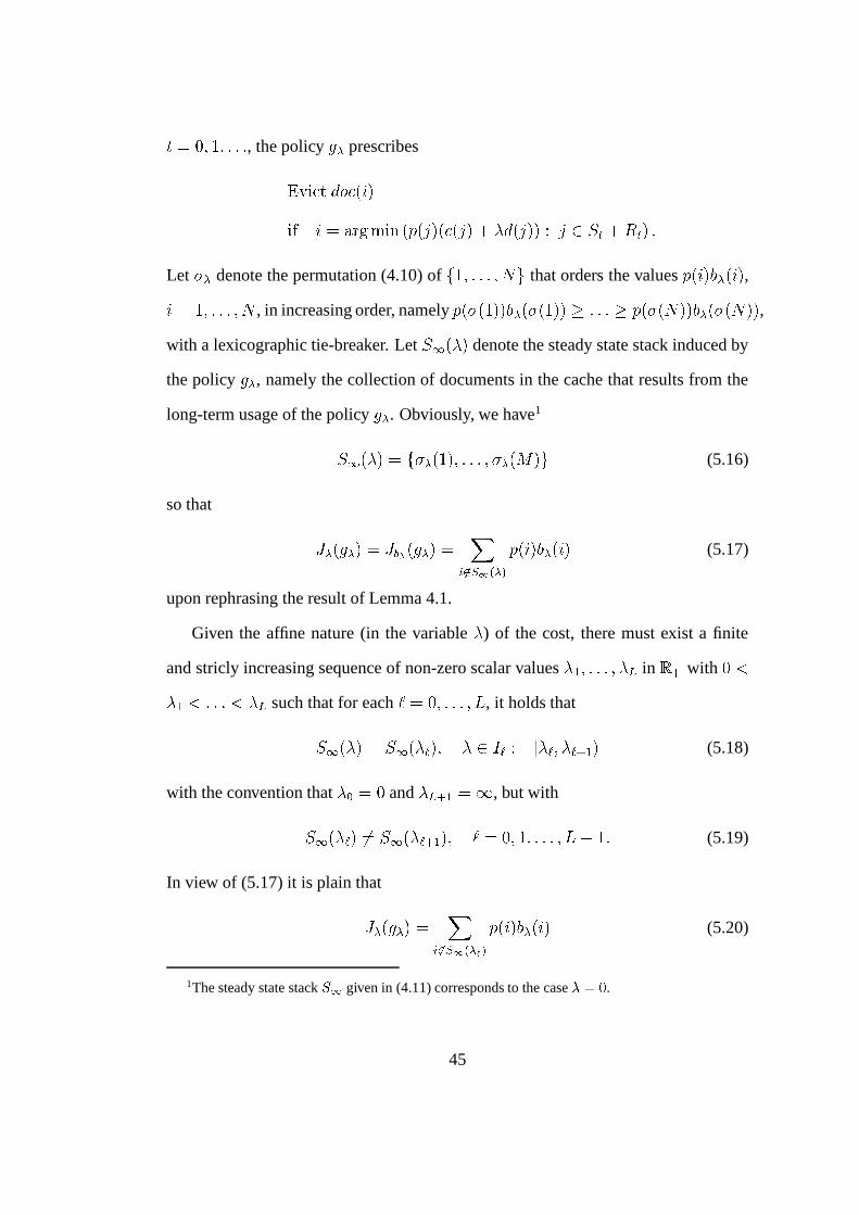
��� ����� � ����� �� ��� � ����� ���*��� ���� � ������ � � ���� � � � � � � � � � �
Let � � denote the permutation (4.10) of � ��� � � ����� that orders the values � ��� � � ���� � ,� �3��� � � ��� , in increasing order, namely � � � � /� � � ��� � � /� ��� � � �� � � � � � � � � �� � � � � � ,with a lexicographic tie-breaker. Let � � � � denote the steady state stack induced by
the policy ��� , namely the collection of documents in the cache that results from the
long-term usage of the policy ��� . Obviously, we have1
� � � � � � � ��� /� �� � � � � ��� �6� � (5.16)
so that
� ��������� � ����� ������� ��
����� � � � ��� � � ���� � (5.17)
upon rephrasing the result of Lemma 4.1.
Given the affine nature (in the variable�
) of the cost, there must exist a finite
and stricly increasing sequence of non-zero scalar values� ���� � � �� ���
in � with � �� ���6 � � � ���
such that for each� �)��� � � ���� , it holds that
� � � � � � � ��� � � � � � � � � � ��� � ��� �� � (5.18)
with the convention that� � �)� and
��� �� � � , but with
� � ��� � � � � ��� �� � � � �)������ � � ���� ��� (5.19)
In view of (5.17) it is plain that
� ��������� ��
����� � ��� � ��� � � ���� � (5.20)
1The steady state stack� � given in (4.11) corresponds to the case ��� .
45

whenever�
belongs to the interval � � for some� � ������ � � ���� . These facts are
described through an example in Figure 5.1, in which � � � , � � 0 , the cost
vectors are � � � �� 0���� � and � � ���� '&���� '0�&�� , and the reference pmf is given by
� �$� /.����/.����/.�� � .
Proof of Theorem 5.1. For each policy � in , the quantities � ��� � � and � ��� � � are
non-negative as the one-step cost function � and are non-negative. Thus, the map-
ping� � �
� ��� � � (5.3) is non-decreasing and affine, and we conclude from (5.13) that
the mapping� � � ��������� is indeed non-decreasing and concave. Its piecewise-linear
character is a straightforward consequence of (5.20).
In order to proceed we make the following simplifying assumption:
Assumption (A) If for some� � � it holds that � ��� � � ���� �"� � ���� � ����� for some
distinct � ��� � ��� � � ��� , then there does not exist any � � � ��� with � � ��� � � ��such that � ��� � � ���� � � � ���� � ����� ��� � � � � ��� � � .This assumption can be removed at the cost of a more delicate analysis without af-
fecting the essence of the optimality result to be derived shortly.
For each� � ������ � � ���� , the relative position of the quantities � ��� � � ����� � � � �
��� � � �� , remains unchanged as�
sweeps through the interval � ��� � ��� �� � . Under
assumption (A), when going through� � � � �� , a single reversal occurs in the relative
position with
� � ��� � � � � ��� � /� �� � � � � ��� � � ��/� � � ��� � �6� � (5.21)
and
� � ��� �� � � � � ��� � /� �� � � � � ��� � � ��/� � � ��� � � �(/� � (5.22)
46

Figure 5.1: An illustration of the intervals ��� , ���������� � � ���� , with ����� , and the
resulting optimal average cost � ���������
47

By continuity we must have
� � � ����� �6� � � ��� � � � � ����� �6� � ��� � � ��� � � �(/� � � ��� � � � � ��� � � �(/� � (5.23)
Theorem 5.2 Under the foregoing assumptions, the mapping� � � ��������� is a non-
increasing piecewise constant function on � .
Proof. The analog of (5.20) holds in the form
� ��������� ��
����� � ��� � ��� � ��� � (5.24)
whenever�
belongs to � � for some� �)��� � � ���� . Hence, the mapping
� � � ��������� is
piecewise constant.
Now pick� �)������ � � ���� � and consider
�and � in the open intervals � � � � ��� �� �
and � ��� �� � ��� � � , respectively. The desired monotonicity will be established if we can
show that � ������� �� � ��������� �,� . First, from (5.24), note that
� ����������2� ��������� ��
� �� � � � ��� � ��� � � �� �� � � � ��� � ��� � (5.25)
� � � � ��� �6� � � � �� �6� � � � � � ��� � �(/� � � � ��� � �(/� �given the steady state stacks (5.21) and (5.22), as we recall that � � � �4� � � ��� �and � ��� � � � � ��� �� � .
Next, pick ���2� such that� ��� and � ��� are still in the open intervals � � � � ��� �� �
and � ��� �� � ��� � � , respectively. By (5.20) we get � � � ����� � � � � � and
� ��� ������� �� � �������� ��
����� � ��� � ��� � � ��� ��� �� ������ � � � ��� � � ���� �
��
����� � � � ��� � � ������� � � ������ � � � ��� � � ���� �
� ��
����� � � � ��� � ��� � (5.26)
48

Similarly,
� � ������� � ��2� � ������� � ��
����� � � � ��� � ��� � (5.27)
By Theorem 5.1, the mapping� � ����������� is concave , hence
� � ������� � ��2� � ����� � �6� ����������� � � � ��������� Making use of (5.26) and (5.27) in the last inequality, we readily conclude that
�� �� � � � ��� � ��� � � �
� �� � � � ��� � ��� � (5.28)
But � � � � � ��� ��� � and � ��� � � ��� ��� �� � , whence (5.28) is equivalent to
� � � ����� �6� � � � ����� �6� � � � � � ����� � �(/� � � � ��� � � �(/� � (5.29)
The desired conclusion ��������� �� � ��������� �(� is now immediate from (5.25).
5.4 The constrained optimal replacement policy
We are now ready to discuss the form of the optimal replacement policy for the con-
strained caching problem. Throughout we assume Assumption (A) to hold. Several
cases need to be considered:
Case 1 - The unconstrained optimal replacement policy � � satisfies the constraint,
i.e., � ����� � � � - , in which case � � is simply the optimal replacement policy � �� for
the unconstrained caching problem, associated with the generic cost � . This case is
trivial and requires no proof since by Theorem 4.1 the average cost is minimized and
the constraint satisfied.
49

Case 2 - The unconstrained optimal replacement policy does not satisfy the con-
straint, i.e., ������� � � � - , but there exists� �6� such that ����������� � - . Two subcases
of interest emerge in this context and are presented in Theorems 5.3 and 5.4 below.
Case 2a - The situation when the policy � � above saturates the constraint at level
- was covered earlier in the discussion; its proof is therefore omitted.
Theorem 5.3 If there exists� �3� such that � ��������� � - , then the policy ��� can be
taken as the optimal replacement policy � � for the constrained caching problem (and
the constraint is saturated).
Case 2b - The case of greatest interest arises when the conditions of Theorem
5.3 are not met, i.e., ������� � �4� - , � ������� � � - for all � �5� but there exists� �+�
such that � ��������� � - . In that case, by the monotonicity result of Theorem 5.2, the
quantity
�� � ����� � � �,� � � ��������� � - � (5.30)
is a well defined scalar in � ������ . In fact, we have the identification
� � � ��� � � (5.31)
for some� �,������ � � ���� �2 , and it holds that
� ��������� � � ��� - �)� ��������� � (5.32)
For each � in the interval � ��� � , define the Markov stationary policy���
obtained
by randomizing the policy ����� and ����� � � with bias � . Thus, the randomized policy���
prescribes
��� ����� � ����� �
� ��� �
��� �� ����� ����� � ���� � �������� � � � � ��� � � � w.p. ������ ����� � ���� � ��� � � ����
� � � � � � � ��� w.p. � � (5.33)
50

Theorem 5.4 The optimal cache replacement policy � � for the constrained caching
problem is any randomized policy���
of the form (5.33) with � determined through
the saturation equation
� ��� � � � � - (5.34)
Proof. For the most part we follow the arguments of [13]: Let� �$������ � � ���� �,
be the integer appearing in the identification (5.31). Pick�
and � in the open interval
� ��� � ��� �� � and � ��� �� � ��� � � , respectively, in which case
��� ������� and ��� �(����� � � (5.35)
with
� ������� � � - �)� ��������� (5.36)
Thus, as in the proof of Theorem 4.4 in [13], let�
and � go to��� �� monotonically
under their respective constraints. The resulting limiting policies � and � (in the
notation of [13]) are simply given here by � �(� ��� � � and � ������� with 2
���� � � � � ��� ������� � � � ������������ � (5.37)
for every � in the interval � ��� � , and the optimality
��� � � � � �6���� � � � � � (5.38)
follows. Moreover, the mapping � � � ��� � � � being continuous [52], with ����� � � � � � � �� ��������� � � � and � ��� � � � � ��� � � ��������� � , there exists at least one value � in � ���/� such that
2See details in the proof of Theorem 4.4 in [13].
51

(5.34) holds. The proof of optimality is now complete in view of comments made in
Section 5.3.
It is possible to give a somewhat explicit expression for � ��� � � � for � in � ��� � .
Lemma 5.1 Let � � denote the set of documents that are never removed from the
cache once requested, namely
� � � � � � ��� � � � � ��� �� � � � � ��� � /� �� � � � � ��� � � ��/� � (5.39)
The average cost ����� � � � can then be expressed as
� ��� � � � � � � � �*� � � ������� # �(
����� � ���� � � � � �� � � � � � � ��� (5.40)
with
������� #��(
����� � ���� � � � � � � � � � � � � � �
��� �� � � ��� � ��� � � � ��� � � � � ����� �6� � � � ����� �6� �� � � � ��� � � � � � ��� � � �(/� � � � ��� � � �(/� � � (5.41)
where � ��� � represents the asymptotic fraction of time that the cache contains the
document � ����� �6� , and is given by
� ��� � � � � � � � ����� �6� �� � � � � ��� � �6� � �)� � � ��� � � � ��� � � �(/� � (5.42)
Proof. Under the policy� �
and i.i.d requests, if the document � ��� � �6� is in the cache,
it can only be removed from the cache when � ����� � �%/� is requested. The time
52

until the eviction of � ����� �6� is therefore a Geometric rv (of type II) with parameter
� � � � � � � � ����� ���)/� � . Similarly, if � ����� ���)/� is in the cache, the time until its
removal is a Geometric rv with parameter � � � � � ��� � �6� � . The fraction of time that
� ����� �6� is in the cache, is then simply
� ��� � ��� � � � � � � �� �� � ��� � �� � � � � � � �� �� � ��� � � �� � � � � � � �� � �
� � � � � � ��� � �6� �� � � � � ����� �6� � �)� � � ��� � � � ����� � �(/� � �
and (5.41) follows.
Case 3 - Finally, assume that ����������� � - for all� � � . This situation is of
limited interest as we now argue: Fix� �(� . For each policy � in , we can use the
optimality of ��� to write
- � � � � ����������� ��� ��������� � � � � ����� � � ��� ��� � � (5.43)
Thus, letting�
go to infinity, we conclude that
- �6� ��� � � � � � (5.44)
The constrained caching problem has no feasible solution unless there exists a policy
that saturates the constraint. Typically the inequality above will be strict.
53

54

Part II
Modeling and Measuring Internet
Cache Consistency and Quality of
Data
55


Chapter 6
Internet Cache Consistency
6.1 The cache consistency problem
The discussion in Part I of the dissertation implicitly assumes that server documents
are never modified. In other words, the content of documents at the server remains
fixed over time. This operational assumption does not hold in practical Web caching
systems.
A cached object is termed consistent if it is identical to the master document, at
the time it is served to the user from the cache. The consistency model in use reflects
the degree to which cached replicas are kept consistent. In order to increase document
consistency, Web servers and Internet caches employ consistency algorithms that
invalidate cached copies upon freshness expiration. Each user request that finds an
invalid copy is forwarded to the server, which sends a fresh object back to the user,
and the stale cached replica is replaced with the latest version.
In reality, Web pages are updated at rates that are determined by the application
of the hosting server, the services offered in each document, as well as the rollout
57

schedule for the production server. Consistency assurance becomes more challenging
when server documents are updated rapidly (e.g., weather updates, sports scores,
news portals), since frequent server-cache communications are required to properly
track the freshness at the cache. Furthermore, since all communications between the
server and the cache are subject to constraints imposed by the network infrastructure,
consistency is impeded by the network transmit delays. This fact is noticeable in
wireless applications, mobile devices, and satellite systems, where the non-negligible
communication latency can significantly impact the QoD [72].
6.2 Consistency algorithms on the Web
Consistency issues have been extensively studied in distributed shared memories
[47], hierarchical virtual memories [63], network and file sharing systems [48], and
distributed databases [30]. In spite of this fact, analytical models and consistency
metrics developed for those earlier systems cannot be applied toward the performance
evaluation of Web consistency algorithms in a straightforward manner; operational
rules pertaining to those systems do not coincide with those used on the Web.1
On the Internet, algorithms fall in one of three categories, namely Time-To-Live
(TTL), client polling, and server invalidation. Operational principals characterizing
algorithms in each category are now described below.
1Additional details regarding individual system characteristics and (dis)similarities to Internet
caches can be found in [18, 35, 42] and their references.
58

6.2.1 TTL algorithms
When TTL algorithms are employed, each document accepted by the cache is equipped
with a Time-To-Live (TTL) parameter, which is either provided by the server or de-
termined at the cache. Once a document is placed in the cache, it is considered valid
until the time specified by the Time-To-Live elapses. A user request that finds a valid
cached copy incurs a cache-hit and is served directly by the cache. On the other hand,
requests presented after the Time-To-Live has expired, are cache-miss requests that
are forwarded to the server, which in turn sends a fresh copy to the cache, and from
there to the user.
TTL algorithms are widely implemented in general Internet applications, e.g.,
DNS, FTP, and HTTP caches [21, 40, 55, 56]. This fact is a direct consequence of
their simplicity, sufficiently good performance, the flexibility to assign a TTL value
to a single cached data item, and the ease of deployment in hierarchical caching sys-
tems [34]. In the literature, several TTL protocols are available, with each algorithm
utilizing a distinct Time-To-Live calculation technique. Commonly encountered al-
gorithms include the fixed TTL whereby the Time-To-Live is always set to a constant
# [21, 22, 23, 24, 34, 40], the LM-Factor used in Squid caches that calculates the
Time-To-Live based on the last master modification time [18, 77], and the non-causal
perfect TTL (also referred to as the optimal TTL algorithm or precise-expiration pro-
tocol) according to which the Time-To-Live expires at the exact moment of next
master update [44, 54, 79].
59

6.2.2 Client polling
A client polling consistency algorithm is invoked according to a schedule that is
dictated by the cache. Each time it runs, the algorithm connects to the server and
initiates an If-Modified-Since request, accompanied by the identifiers (i.e., validators
[28]) of one or more cached items. Commonly used validators include the Last-
Modified-Timestamp, document version, header, and the entity-tag (ETag). If the
server finds that the value of the validators match those of the master (i.e., the cached
copy is up to date), it sends a 304 Not-Modified reply to the cache, and the cache
continues to serve the valid copy in response to user requests; otherwise the server
returns a 200 OK message together with the latest master version, and the stale cached
copy is replaced with the new download.
Practical implementations of client polling protocols include the if-modified-since
algorithm (also known as the polling-every-time protocol) under which every request
that arrives to the cache prompts an If-Modified-Since message to the server, the
periodic-polling method that connects to the server every�
time units [57], and the
piggyback-cache-validation whereby freshness control messages are embedded in
other (i.e., non-consistency related) transmissions to the server.
In spite of their simplicity, polling algorithms are not favored in general Internet
applications. The if-modified-since algorithm clearly results in good QoD, but can
significantly increase the server and network loads, and user-service latency [79].
Other client polling protocols that are less resource intensive than the if-modified-
since algorithm typically result in poor cache consistency.
60

6.2.3 Server invalidation
Server invalidation algorithms are invoked by the server upon each update to the
master (or shortly thereafter). Once launched, the algorithm connects to one or more
caches that contain a copy of the modified document, and informs each cache of the
changes. Some algorithms perform this notification by sending a new master copy
to the cache. Other algorithms only invalidate the stored copies, and the first request
that arrives after the invalidation is a cache-miss that is forwarded to the server.
Invalidation protocols are implemented in many commercial Web caches, and are
particularly popular in servers that contain dynamically generated Web pages. Com-
mon protocols include the replication algorithm that forwards the master changes to
all caches immediately after the update [79], the invalidation-report used in wire-
less and mobile applications to inform end-user caches of content updates [80], as
well as the piggyback-server-invalidation under which the invalidation messages are
encapsulated in non-consistency related communications with the cache [45].
The main advantage of invalidation algorithms lies in the high degree of cache
consistency attained by most protocols in this category. However, other (e.g., TTL)
consistency solutions are preferred in general, since a server that employs an invali-
dation algorithm must maintain a list of all system caches.
6.3 Weak vs. strong consistency models
In order to capture the freshness of a cached item with respect to the master, we find
it useful to introduce the following freshness classification: A server-fresh document
is defined as the latest serviceable document at the server, whereas a cache-fresh doc-
ument is defined as a valid cached copy, or equivalently, as one thought to be server-
61

fresh by the cache. We define a cache-fresh* document as one that is both cache-fresh
and server-fresh, and a document that is not cache-fresh* is termed cache-stale*.
The schedule of the consistency algorithm and the non-zero server-cache trans-
mit delay � make it possible for a cached item to be considered valid by the cache
despite the availability of a later (i.e., fresher) version at the server. Such occurrences
would result in the undesirable download of cache-stale* (thus inconsistent) docu-
ments from the cache. Following Cao and Liu [18], strong consistency algorithms
are characterized by users being served strictly server-fresh documents under zero
delays and processing times. A consistency algorithm that is not strong is termed
weak, in which case there is a possibility that users download inconsistent copies
(i.e., ones that are cache-fresh yet not server-fresh), even under zero delays.
In general, causal TTL and most client polling algorithms are weakly consistent,
whereas the if-modified-since, the perfect TTL, and most server invalidation proto-
cols are strongly consistent. To appreciate this fact, consider the fixed TTL and the
if-modified-since algorithms, when all delays are zero:
� With the fixed TTL algorithm, each document placed in the cache remains valid
for # time units, and all requests presented until the TTL expiration are served di-
rectly from the cache. If the master is updated prior to the expiration, then all requests
that arrive after the update yet before the TTL has expired are served with a cache-
stale* copy. The fixed TTL is therefore a weak consistency protocol.
� The if-modified-since algorithm sends a conditional GET directive to the server
in response to every user request that arrives to the cache. If the server finds that
the cached item is fresh, a 304 Not-Modified message is returned to the cache; oth-
erwise the server forwards the latest master version and the new object is loaded
into the cache. Either way, once the server-cache communications complete, the re-
62
quested document is sent to the user from the cache. If � ��� (i.e., instantaneous
transmissions) then users are always served with server-fresh copies, hence the if-
modified-since is a strong consistency protocol.
6.4 Quantifying cache consistency and QoD
For a given consistency algorithm, we define a cache-hit* as a cache-hit that results
in a server-fresh download from the cache to the user. The complementary situation
of a cache-stale* download is termed a cache-miss*. Each cache-hit* is therefore
a cache-hit, but the reverse clearly does not hold. The hit rate and the hit* rate are
then the long-run average download rates of cache-fresh and cache-fresh* documents
from the cache, respectively. Since each cache-hit* is necessarily a cache-hit, the
hit* rate can never exceed the hit rate, and equality is achieved for strong consistency
algorithms if �+�,� .The hit* rate is most useful for measuring the fraction of fresh downloads when
the cache utilizes weak protocols, for then the likelihood that users retrieve stale ob-
jects is potentially large: Consider the fixed TTL algorithm when # is very large,
and server documents are updated frequently. A large value for # guarantees a high
hit rate and lowered bandwidth utilization [34, 40], but results in poor quality of data
(QoD), even when the communication latency is negligible (e.g., broadband connec-
tivity). Measuring consistency is also important for strong consistency mechanisms
deployed in a hierarchy of caches, or when the delay is large (e.g., satellite and wire-
less networks [67, 80]), as previously concluded in [73].
In order to evaluate the consistency performance under a given protocol, we for-
mulate a framework that allows consistency issues to be investigated in a quantitative
63

manner. This framework is presented in Chapter 7, where the focus is on a single
server-cache pair and a single data object, as we attempt to isolate relevant issues.
User requests and master updates are modeled by mutually independent point pro-
cesses. Then, the hit and hit* rates of any given consistency algorithm can in prin-
ciple be evaluated, and various design parameters could be tuned on the basis of the
resulting performance.
In Chapters 8 and 9, we apply the modeling framework to the analysis of the
fixed and perfect TTL algorithms, respectively. Hit rate and hit* rate results are
obtained for each protocol under any value of the download delay � ��� . Closed
form expressions for the calculated rates are available in some special cases when
the requests are generated according to a Poisson process. Computable bounds are
derived for each algorithm when the request process is a renewal process, and are
tightened when the inter-request time distribution belongs to certain subclasses of
distributions (e.g., IFR, DFR, NBUE and NWUE). On the basis of these results,
we can now explore the degradation of the hit and hit* rates as a function of the
communication delay � , and of additional algorithm-specific parameters.
To conclude, we note that the proposed modeling framework can also be used
to investigate consistency issues in polling and invalidation algorithms, as well as
techniques employed by other distributed systems (e.g., virtual shared memories and
file sharing systems [1, 35, 63]).
64

Chapter 7
A Framework for Measuring Cache
Consistency
7.1 The system model
The system is made up of a site called the origin where the current authoritative
version of the data is maintained, and of requestors. Each requestor is identified
with a cache that is used either by users or by client-caches. Thus, the origin and
requestors are synonymous with server and caches, respectively.
Caches are assumed to be of infinite size, reflecting the fact that storage is ample.
The need to specify a replacement policy is moot, and only the operational rules of
the consistency algorithms matter. In particular, once a document has been placed in
the cache, a copy is always available at the requesting cache, although said copy may
be either fresh or stale at any given time.
Under these circumstances, there is no loss of generality in abstracting a caching
system into a single cache-server pair, and in considering a single cacheable data
65

item, say�
, in isolation, as we do from here on.
7.1.1 Modeling requests
User requests for the document�
arrive according to a point process ��# �� ��� ������� � � � with the understanding that the � � request occurs at time # �� . Thus, # �� �# �� �� for each � �������� � � with # �� �5� . Let � � � �� ��� �������� � � � denote the se-
quence of inter-request times with ��� ��"��# �� �� � # �� for each ��� ������ � � . The
point process ��# �� ��� � ������ � � � is assumed to be simple in that � � �� �$� a.s. for
� �,������ � � � so multiple requests cannot occur simultaneously.
As customary, the counting process � � � � � � � � � � associated with the point
process ��# �� ��� �,������ � � � is given by
� � � � � ����� ��� �)������ � � � # �� � � � � ���(� (7.1)
so that � � � � counts the number of requests in the interval � �� � � . The corresponding
residual lifetime process � ����� � � � ���,� � is defined by
����� � � �(#�� � � �� � � � ���(�
If # �� � � �(# �� �� for some � �3������ � � , then � � � � �� and ����� � � � # �� �� � � , i.e.,
����� � � represents the amount of time that will elapse until the occurrence of the next
request after time � .We assume at minimum that the point process ��# �� �� �%������ � � � admits a rate
in the sense that there exists a finite constant� � �2� given by the limit
� � � ����� �� � � � �� � ���
We refer to� � as the request rate.
66

7.1.2 Modeling document updates
The document�
changes over time, and is updated according to the second point
process ��#� � � � � ������ � � � where #� � is the epoch at which the � � update takes
place. We denote by � � � ���� � � ������ � � � the sequence of inter-update times with
� � �� � # � �� �(# � for each � � ������ � � . Here as well, # � � # � �� for each
� �%������ � � with #� � �$� . The point process ��# � � � �$������ � � � is assumed to be
simple so that multiple updates are ruled out.
In analogy with (C.8), the counting process � �4� � � � � ��� � associated with the
point process ��# � � � �,������ � � � is given by
�4� � � � ����� � � �)������ � � � # � � � � � ���,�
with �4� � � counting the number of updates in the interval � �� � � . The corresponding
residual lifetime process � � ��� � � � ���,� � is defined by
� ��� � � �(# � � � �� � � � ���(�
so that � ��� � � represents the amount of time that will elapse until the next update after
� .As before, we assume that the process ��# � � � �,������ � � � admits a rate, referred
to as the update rate, in the sense that there exists a finite constant�
� �2� given by
�� � ����� ��
�4� � �� � ���
7.2 Basic assumptions
Throughout, the point processes ��# �� ���5� ������ � � � and ��# � � � � ������ � � � are
assumed to be mutually independent. This reflects the lack of correlation between
user behavior and the evolution of data content.
67

For reasons of brevity and mathematical simplicity, these point processes are as-
sumed to be renewal processes. For the requests, this means that the inter-request
times � � � �� � � �)������ � � � form a sequence of i.i.d. rvs distributed according to the
common cdf� � . Let � denote any rv distributed according to
� � . Similarly, when
the update process is a renewal process, the inter-update times � � � ���� � �)������ � � �form a sequence of i.i.d. rvs distributed according to the cdf
�� . We denote by �
any rv distributed according to�
� . The cdfs� � and
�� are assumed to have finite
mean � � � � � and � � � � � , in which case it is well known [69] that� � � � � � � � � �
and�
� � � � � � � � � .Let � � � denote the fixed download delay of
�over the network, i.e., if a
document is sent from the server at time � , it is received by the cache at time � � � , at
which point it is ready for access by the users. In the other direction, communication
from the cache to the server is deemed instantaneous as it entails the transmission of
very short control messages.
7.3 Hit rates and QoD
With a given consistency algorithm, we can associate the two performance measures
mentioned earlier, namely the hit and hit* rates. These metrics reflect the quality (or
freshness) of�
from two different viewpoints, namely cache freshness and server
freshness, and capture the fraction of hit and hit* occurrences out of all user requests,
respectively.
In order to count the number of cache-hit instances under the network delay � ,
an � -valued validator process ����� � � � � � � � � is introduced to track the cache
freshness of the cached copy of�
; a hit occurs at request time # �� if and only if
68

� � ��# �� � � ��� . The hit rate is then simply defined by
� � �!� � ����� �� �
��� ��� � � � ����#
�� � � ��� � (7.2)
Similarly, in order to identify cache-hit* requests, the server freshness of the
cached version of�
is monitored through another � -valued process ��� � � � � � � � �� � , so that a hit* occurs at request time # �� if and only if � � � ��#
�� � ���,� , and the hit*
rate is defined as
� � � �!� � ����� �� �
��� ��� � � � � � ��#
�� � � ��� �� (7.3)
The limits in both (7.2) and (7.3) are taken in the a.s. sense and are assumed
to exist with� � �!� and
� ��� �!� constants. This will be the case for all algorithms
considered in this work. In that case, the a.s. limit
����� �� � �
� ��� � � � �
� ��#�� � � ��� �� �
� ��� � � � ����# �� � � ��� � � � ��� �!�� � �!� (7.4)
also exists as a constant. This ratio represents the fraction of server-fresh hits out of
all hits, and therefore measures the QoD produced by a given algorithm.
7.4 Requests and updates in applications
The experimental validation of the proposed model has already been carried out in
numerous studies for the case of � �$� (e.g., see [10, 27, 60, 62, 67, 79] and refer-
ences therein). In these studies, request epochs and update timestamps are extracted
from log files of popular caches in order to calculate the total number of hit* occur-
rences among all user requests.
The selection of the distributions� � and
�� that best models arrivals and updates
is specific to each Internet application. Inter-request times in HTTP and FTP caches
69

follow the Weibull and Pareto heavy tailed distributions, as reported in [27, 62] and
emphasized by Bestavros et al. in [10]. Locality of reference, whereby recently
accessed documents are likely to be shortly requested again, can be (partially) ex-
pressed through an appropriate selection of� � [29, 64]. Web pages that contain
stocks and weather information on the Yahoo portal are updated periodically every
few seconds [67]; logs collected from news servers [60] and Harvest caches [18]
suggest a bimodal inter-update time distribution.
As we shall later observe, the expressions for the hit and hit* rates for the consis-
tency algorithms analyzed in the next chapters depend crucially on the (non-delayed)
renewal function � � � � � � � � � � � �5� . It is therefore rather difficult (if at all pos-
sible) to calculate these rates for general applications owing to the simple fact that� � � � � � � is not known in closed form except in some special cases (e.g., when �is lattice or uniformly distributed, or for a class of matrix-exponential distributions
[5]). In order to circumvent this difficulty and apply the obtained results in general
applications, we derive distribution-free bounds on the calculated rates with the help
of well known bounds on the renewal function. Bounds on the hit and hit* rates are
then tightened when� � belongs to several subclasses of distributions of interest, as
well as for specific inter-request time distributions.
7.5 Bounds on the renewal function
7.5.1 Distribution-free bounds
Bounds are available for the renewal function associated with any distribution� � .
First, recall that the forward recurrence time rv � � associated with the rv � is dis-
70

tributed according to
� � ��� � � � � � �� �� � � �3� � � � � ���(� (7.5)
Lorden [50] has shown the upper bound� � � � � � � � � � � � � ����� � ��� �2�� ���(� (7.6)
while Marshall [53] proved the lower bound� � � � � � � � � � �� � � ��� � � � � � � ����� ���(� (7.7)
We refer to these results as distribution-free bounds as they only depend on the first
and second moments of the distribution� � . These bounds may not be useful when
� ��� � � � � or � � ��� � � � are large for then there is a risk that the upper bound (7.6) is
too loose, or the lower bound (7.7) close to zero for � � � � � � (hence useless).1
To avoid the technical challenges associated with the distribution-free bounds
(7.6) and (7.7), we now seek alternative bounds that do not suffer from the dis-
advantages mentioned above. We achieve this goal by focusing the discussion on
subclasses of distributions of interest (i.e., ones that are commonly used in network
traffic modeling), for which tighter bounds are known to exist.
7.5.2 NBUE and NWUE distributions
A distribution� � defined on � ������ is said to be Increasing Failure Rate, denoted
IFR, if the mapping
� � � � �3� � � � �� � �3� � � � ���(� (7.8)
1 ������ � ����� always since this is equivalent to ������������� . Similarly, ��� �! #"%$'&(" � � $ is a
simple consequence of (7.5).
71

is non-increasing in � for each � � � . Conversely, if the mapping (7.8) is non-
decreasing then� � is termed Decreasing Failure Rate, or DFR in short.2
If a distribution� � on � ������ satisfies the condition
� � ��� � � � � � � ��� � � � ���(��
then� � belongs to the class of New Better Than Used in Expectation (NBUE) dis-
tributions, and the associated renewal function is bounded from above by� � � � � � � � � � � � ���(� (7.9)
On the other hand, when
� � ��� � � � � � � ��� � � � ���(��
then we say that� � is New Worse Than Used in Expectation (NWUE). In this case,
the corresponding renewal function is bounded from below by� � � � � � � � � � � � ���(� (7.10)
It is well known [12] that if� � is IFR (equivalently, DFR), then it is also NBUE
(equivalently, NWUE).
To summarize, if� � is either IFR or NBUE, then the following bounds on the
renewal function are readily available from (7.7) and (7.9), namely
� � �� � � ��� � � � � � � � � � � � � � � � � ���(� (7.11)
In a similar manner, the combination of (7.6) and (7.10) for� � NWUE yields
� � � � � � � � � � � � � � � � � ����� � � � ���� ���(� (7.12)
2Much of this material can be found in the monograph by Barlow and Proschan [12].
72

Finally, if� � is DFR, then a tighter upper bound than the one specified in (7.6)
is reported by Brown [16]. Combining the upper bound by Brown with the lower
bound (7.10) gives
� � � � � � � � � � � � � � � �� ��� � � � �0 �2�� ���,� (7.13)
7.5.3 Distribution-specific bounds
Linear bounds on the renewal function are presented by Marshall [53]. These bounds
are specific for each given distribution and can be used to further improve the bounds
on the renewal function listed thus far.
For a given distribution� � on � ������ , define
� � � ������ ��� � � � � � � � � � ��� � � � � � � � � � � � � (7.14)
and
�
� ������ ��� � � � � � � � � � ��� � � � � � � � � � � � � (7.15)
where �)� � � �,� � � � � � � � �6 � . Then, the renewal function associated with the
distribution� � is bounded from above by� � � � � � � � � � � � �
� (7.16)
and from below by � � � � � � � � � � � � � �(7.17)
for all values of ���,� .Previous comments regarding NBUE and NWUE distributions allow the linear
bounds (7.16) and (7.17) to be sharpened: Whenever� � is NBUE we have
� � � � � � � � � � � � � � � � �
� ���(�� (7.18)
73

and whenever� � is NWUE we conclude
� � � � � � � � � � � � � � � � � � � ���(� (7.19)
7.6 Poisson, Weibull, and Pareto requests
The Poisson, Weibull, and Pareto distributions are often used to model time gaps in
network packet arrivals, as well as inter-request times experienced by Web caching
systems. Consequently, special attention is given to evaluating the hit and hit* rates
under these inter-request time distributions, for each of the algorithms examined in
the following chapters.
Poisson requests. Poisson requests correspond to the generic inter-request time rv
� being exponentially distributed, say with rate� � , i.e.,
� � � � � � ��� ����� � � ���(�
In this case, the renewal function is available in closed form [69] with� � � � � � � � � � � � ���(�
This fact permits the derivation of closed form expressions for the hit and hit* rates,
provided that the inter-update time distribution�
� is also at hand.
Of even greater interest are the Weibull and Pareto distributions, which were
proved more suitable (than the exponential distribution) in representing inter-arrival
times of user requests at the cache [27, 39, 62].
Weibull requests. The Weibull distribution is characterized by
� � � � � � ��� � � � � �� � ���,�� - � � �2��74
with the two first moments given by� � � � � � � � - � � �(/�
and ��� � � � � � � � 0- �(/�
where� � � � is the Gamma function defined through
� � � � �� � � ��� � � � � � � �2�
The residual lifetime rv ��� associated with the Weibull rv � has the distribution
� � ��� � � � �� �
- � � � � - �/� � � ��� � � ���(�
with � � � ����� denoting the lower incomplete Gamma function given by
� � � ����� �� �� � ��� � � � � � � ���� � �(�
It is well known [12] that the Weilbull distribution is DFR for - � . Thus, the
DFR bounds in (7.13) can now be used to obtain bounds on the renewal function
associated with the Weibull inter-request time distribution, in the process yielding
� � � � � � � � � � � � � � � �� ��
0 � � � � � 0- ��2�� ���,�
On the other hand, when - � the Weibull distribution is IFR [12], and the appro-
priate IFR bounds (7.11) provide us with
� � � � � �
- � � � � - �/� � � ��� � � � � � � � � � � � � � � ���(�
Here, the Marshall bounds (7.16) and (7.17) are omitted by the simple fact that�
�� for - �) and
� � � � whenever - �6 , so the resulting bounds are less effective
than those listed above.
75

Pareto requests. Similar arguments apply to the Pareto inter-request time distribu-
tion defined by
� � � � � �� � � �� � � � � � ���(�� - � � �2�
This distribution is DFR, and we restrict the discussion to - �30 , in which case the
first two moments � � � � � �- �2 (7.20)
and ��� � ��� � 0 � �� - � 0�� � - ��/�
are finite. In this case, the distribution of the residual lifetime rv � � is given by
� � ��� � � � �3 � � �� � � � �
� �� ���(�
It is a simple matter to check that the DFR bounds in (7.13) yield
� � � � � � � � � � � � � � � - � 0 � ���,� (7.21)
In addition, since�
�3 in the Marshall bound (7.18), alternative bounds are readily
available in the form
� � � � � � � � � � � � � � �(�� ���(� (7.22)
Upon making use of these results, we conclude that
� � � � � � � � � � � � � � �� ��� � - � 0 �� � � ���,�
for all values of - ��0 .
76

Chapter 8
The Fixed TTL Algorithm
8.1 Operational rules of the fixed TTL
With the nomenclature introduced in Chapter 7, the fixed TTL algorithm can be de-
scribed as follows: Whenever the server receives a request for�
, say at time # �� for
some � �3������ � � , it returns the current version together with the TTL field #%�6� .The first miss request for
�arrives to the cache at # �� ��� , and the cache makes the
returned version available at # �� �2� . Any subsequent request for�
at the cache in
the time interval ��# �� �,� � # �� �)� ��# � is served directly from the cache without
contacting the server.
If a request at time # �� for some � � �� 0��� � � is the first one presented after the
TTL has expired, then it is forwarded to the server, in which case requests arriving
during the interval ��# �� � � � # �� � � � # � are all hits. The discussion is carried out
under the assumption that the requests presented in ��# �� � # �� �(�!� for � �������� � � ,are sent to the server as well. However, the copies of
�received in response to these
requests are neither placed nor do they reset the TTL, as assumed in [18] for the
77

empirical evaluation of various TTL algorithms.1
8.2 Zero delays
In this section we drop � from earlier notation as it is now set to zero. Cache fresh-
ness of the object�
is completely described by the validator process ��� � � � � � �� � , which continuously tracks the TTL value at the cache. The process has right-
continuous sample paths with left limits, and is defined by
� � � � �%� � ��#�� ��(� � � # �� � � � #
�� � ��� # �� ��
for each � �)������ � � , with the update rule
� ��#�� � �
��� �� # if � ��# �� � � �,�� ��# �� � � if � ��# �� � � �2� (8.1)
Operational assumptions made earlier lead to the initial condition � � � � � � � so
that � � � � � # by (8.1). The timer will have expired at time � � � if and only
if � � � � � � � . Thus, the � � request at time # �� produces a hit if � ��# �� � � � � ;otherwise it will be a miss. The hit rate2 � ��# � for the fixed TTL is now as defined in
(7.2). Its evaluation has been carried out already by Jung et al. [40].
Proposition 8.1 If the point process ��# �� �� � � �,������ � � � is a renewal process, then
it holds that � ��# � � � � � ��# � � � � � � � ��# � � �
1We restrict the analysis to the case � ��� , as customary on the Web.
2The notation � ����� is used here to reflect the dependency of the hit rate on the fixed TTL param-
eter � .
78
Note that� � � ��# � � ��� � � � ��# � � for all # ��� as soon as
� � admits a density, a
common occurrence in applications. Proposition 8.1 being a special case of Proposi-
tion 8.3 with �+�)� , its proof is therefore omitted.
As we now turn to the hit* rate, we note that even in the absence of transmission
delays between the server and the cache, there is a possibility that a request incurs
a hit for a stale copy. The consistency of the cached object with that offered by the
server is captured by the process ��� � � � � � � � � � which tracks the time until the
expiration of the cache-fresh* copy. This process has right-continuous sample paths
with left limits, and is defined by
� � � � � �$� � � ��#�� ��(� � � # �� � � � #
�� � ��� # �� ��
for each � �)������ � � , with the update rule
� � ��#�� � �
��� �� ��� � � ��# �� � ��� ����# �� � � if � � ��# �� � � �,�� � ��# �� � � if � � ��# �� � � �2�
The initial condition is taken to be � � � � � � �6� so that � � � � � � ��� ��#���� ��� � � � . The
hit* rate� ����# � is given by (7.3) with ��� � � � � � ���(� � as defined above.
Proposition 8.2 Under the assumptions of Proposition 8.1, it holds that
� � ��# � � � � � � ��� ��#���� � � � � � � � � � ��# � � � (8.2)
provided the point process ��# � �� � � �)������ � � � is also a renewal process.
Proposition 8.2 follows from the analogous result for the general case � �$� given
in Proposition 8.4.
In this last expression the stationary forward recurrence time � � is taken to be
independent of the counting process � � � � � � ���(� � ; its distribution is given by
� � � � � � � � ��
� �� � � ��� ��� � � ���,� (8.3)
79

An alternative expression for� � ��# � follows by specializing (8.8) with � �+� , and
is given by
� � ��# � � � ��# ��� � � � � #�� � ��
� �
� � � ��� � � � � � � � ��# � � � � � � �3� � � �
� � ��# �� ��
� �
� � � ��# � � � � � � � ��� � �� � � ��# � � � �( � � �3� � � � (8.4)
8.3 Non-zero delays
In the presence of a network delay � � � , cache freshness is monitored through
the validator process ����� � � � � � ��� � , which continuously tracks the TTL value at
the cache (see Figure 8.1). This process has right-continuous sample paths with left
limits, and is defined as follows: First, define the � -valued rvs � � ��� � �������� � � �recursively by
� � �� � ����� � � � � � � # ���� � � � # �2# �� � (8.5)
for each � � ������ � � with � � � � . The rv � � identifies the � � request forwarded
to the server that resets the TTL value to # , as we recall that requests made in the
interval ��# ���� � # ���� � �!� are forwarded as well, but do not affect the TTL at the cache
in that interval. For each � �)������ � � we can then write
� � � � � ��� � � ��# ���� � �!� �(� � �(��# ���� � �!� ��� on the interval � # ���� �(� � # ���� � � ���!� , with the update rule ��� ��# ���� �(�!� �$# . We
initially take � ��� � � �)� for � � � ��� , and the hit rate� ��#����!� can be written as in
(7.2) with ��� � � � � � ���(� � .
80

Server updates
L (t)
L *(t) h - hit m - miss h* - hit* m* - miss*
t
m m m m m h,m* h,m*h,m*h,h* h,h*
Cache requests
T
T
Figure 8.1: A time line diagram of requests, updates, and the freshness tracking
processes for the fixed TTL with ���2� .
Proposition 8.3 If the point process ��# �� �� � � �,������ � � � is a renewal process, then
we have
� ��#����!� � � � � � ��# � �!� � � � � � � � � �!� � � � � � � ��#�� �!� � � � (8.6)
for each � �,� .
As expected, this result specializes for �+�,� to the one stated in Proposition 8.1
and in [40]. A proof of Proposition 8.3 is available in Appendix B.
Next, the evaluation of the hit* rate is made possible through the server-freshness
tracking process ��� � � � � � � � � � � at the cache. This process has right-continuous
sample paths with left limits, and is defined as follows: For each � �)������ � � we set
� � � � � � �$� � � � ��#�� � �!� �(� � �(��# �� � �!� � �
whenever # �� � � � ��� # �� �� � � with the update
� � � ��#�� � �!� �
��� �� ��� � � � ��# �� � �!� �/� � ����# �� � � �!� � � � � � � � ��# �� � �!� � � �)�� � � � ��#
�� � �!� � � � � � � � � ��# �� � �!� � � ���
81

The initial conditions are taken to be � �
� � � � �6�� � � � �(� , as illustrated in Figure
8.1. The hit* rate� ����#����!� is given by (7.3), this time with ��� �
� � � � � � � � � , and is
evaluated in the following proposition.
Proposition 8.4 Under the assumptions of Proposition 8.2, we have
� � ��#����!� � � � � � ��� � � � #���� � � � � � � � � � � ��� � � ��� � � � � � � � � � ��#�� �!� � � � (8.7)
for each � �(� .
As before, � � is taken to be independent of the counting process � � � � � � � � � � ,which allows us to rewrite the hit* rate as
� � ��#����!� (8.8)
� � ��#����!��� � � � � #�� � � � ��
� ��
� � � ��� � � � � � � � �!� � � � � � � ��#�� �!� � � � � � ��� � � �
� � ��#����!��� � � � ��� � � ��
� ��
� � � � ��# � �!� � � � � � � � ��� � � � � � � � ��#�� �!� � � � � � ��� ��� �
The result (8.7) reduces to Proposition 8.2 for the case of �5� � . A proof of Propo-
sition 8.4, as well as the derivation of the alternative expression (8.8), are provided
in Appendix B.
8.4 Properties of the hit and hit* rates
Relationships between the derived rates are readily obtained from (8.8) for any value
of � �,� , under the assumptions of Proposition 8.2. The ratio (7.4) that captures the
fraction of non-stale hits satisfies the bounds
� � � � � #�� � � �� � ��#����!�� ��#����!� � � � � � �2� � � (8.9)
82

which clearly show the interplay between network delays and update statistics.
The ability of the fixed TTL to ensure consistency is degraded as the delay in-
creases, as is the case for most algorithms in practice. Better performance can be
achieved by lowering the value of # , yet it is possible that frequent updates prevent
users from ever being served with server-fresh data.3 Furthermore, if documents are
rarely updated, i.e.,�
��� � , then (8.9) implies� � ��#����!� � � ��#����!� as would be
expected.
Key to understanding the performance of practical Web caches under the fixed
TTL algorithm are the effects of # and � on the hit and hit* rates. To do so, we now
focus on monotonicity properties and on the asymptotics of the calculated rates as a
function of these system parameters.
Lemma 8.1 For any inter-request time distribution and fixed delay � ��� , the hit
rate produced by the fixed TTL is a non-decreasing function of # .
The proof of Lemma 8.1 is immediate and is therefore omitted.
Lemma 8.2 Assume that� � � � � and
� � � � � are finite. Then, for each � � � , we
have the asymptotics
������� � ��#����!� �3but
������� � � ��#����!� �)�
3e.g., when the master is updated every � time units in which case ��� � �� �!& � .
83

Proof. Starting with the hit rate, we note by the Basic Renewal Theorem [69] that
����� �� � � � � � � �� � � � (8.10)
and the desired conclusion follows since
������� � � � � ��# � �!� � � � � � � � � �!� �
#�� � � #�� � � � � � � ��# � �!� � � � ���
For the hit* rate, applying the distribution-free bounds (7.6) and (7.7) we get the
inequality � � � ��� � � � � � � � �!� � � � � � ��#�� �!� ��� �
� � � � � ��� � � � �
� � ��#�� �!� � � � � �
which leads to the result
������� � � ��#����!�� ������� � � ��#����!��� � � � � #�� � � � �
�
� ��
� � � ��� � � � � � � � �!� � � � � � � ��#�� �!� � � � � � ��� ��� � �
� ������� �
�
� � ��#�� �!�� ��
� � � � � � ����� � � � � � � ��� � � �
� ������� �
�� � � � � � � � � �
�� � � � �
� � ��#�� �!�� �
This last inequality is a consequence of the assumption� � � � � � � and
� � � � � � � ;
a common occurrence in applications.
Although very tempting, it is erroneous to conclude that either one of the hit or
hit* rates are monotone in � for any given inter-request time distribution� � . This
monotonicity property can be deduced in some special cases (e.g., Poisson requests),
and sufficient conditions for it are provided in the following lemma.
84

Lemma 8.3 Given the TTL parameter # , the hit rate incurred by the fixed TTL is
non-increasing in � on � �� #�� if the inter-request time distribution� � satisfies the
condition� � � � � � � � � � � � � � � � � � ��#�� � � �� � ��#�� � � � � � � �,� ����� � �2#� (8.11)
On the other hand, if� � and the inter-update time distribution
�� satisfy the more
relaxed condition
� � � � ��� � � � � � � � � � �� � � � � � ��� (8.12)
� � � � � � #�� � � � � � � � ��# � � � �� � ��#�� � � � ��� � � �(� ����� � �2#��then the hit* rate is non-increasing in � on � �� #�� .
Proof. The lemma only considers the delay � in the interval � �� #�� , to comply with
the ongoing assumption # �6� that was used throughout the analysis of the hit and
hit* rates.
Observe that if � � �3� � , then� � � ��# � � � � ��� � � � ��#�� � � � � , and the suffi-
cient condition (8.11) immediately ensures� ��#���� � � � � ��#���� � ���(� . To derive the
condition on the hit* rate, we refer to the expression for� ����#����!� in (8.7) and define
� ��#����!� � � � � � ��� ��#�� � ��� � � � � � � � � � � ��� � � ��� � � � �� The desired monotonicity
� ����#���� � � � � ����#���� � � � � is satisfied if� ��#���� � ���
� ��#���� � � ��� for # ��� � �5� � ��� . A closer examination of this requirement
yields
� ��#���� � �� � ��#���� � �
85
� � � � � � ��� � � �(� � ��� � � � � �� � � � � � � �� � � � � � � � � � �2#�� � � ��� � � � � �� � � � � � � �� � � � � #�� � � � � � �2#�� � � ��� � � � � �� � � � � � � � ��#�� � � �� � � � � � � �� � � � � #�� � � � � � ��� � � � � �� � � � � � � � ��#�� � � �� � ��# � � � � � �
� � � � � � � � � � ��� � � � � �� � � � � � � �� � � � � #�� � ����� � ��� � ��#�� � � �� � ��#�� � � � � �
� �
Under the assumption that � � is independent of the inter-request time rv � , this last
inequality is equivalent to the monotonicity condition (8.12).
It is now left to explore the asymptotic behavior of the hit and hit* rates as �becomes very large. Before doing so, it is important to point out that the sufficient
conditions listed in Lemma 8.3 are clearly satisfied when the inter-request time is
exponentially distributed (i.e., Poisson requests).
Lemma 8.4 For each #6��� we have the asymptotics
����� ��
� � ��#�� � ���!� � ��
and
����� ��
� ��#�� � ���!� � 0
The proof of Lemma 8.4 follows similar arguments as those used in the proof of
Lemma 8.2, and is therefore omitted.
86

8.5 Evaluating the hit and hit* rates
8.5.1 Exponential inter-request times
An important special case arises when requests occur according to a Poisson process,
in which case quite explicit expressions are available, namely
����� � � ��#����!� � � � #� � ��# � �!� �(
and
� ���� � � ��#����!� � � �� � ��#�� �!� �( � � � ���*� � � #���� � �� ��� � � ��� � � ��
While a simple closed form expression is available for the hit rate, the hit* rate can be
evaluated in principle once the distribution�
� is specified. For instance, consider the
case when updates occur periodically every � time units. It is plain that� � ��#����!� �
� whenever �4 �6� (as would be expected). However if � �)� , as we recall that
� � is uniformly distributed on the interval � ���� � , simple calculations show that
� ���� � � ��#����!� �� �
0�� � � � ��#�� �!� �(/��� � � �!� � � � � � � � � # � � ���
This expression allows for a comparison between the hit and hit* rates incurred by
the fixed TTL for the practical systems examined in [67], as illustrated in Figure 8.2
for several values of # and � .
8.5.2 Distribution-free results
Bounds presented in Section 7.5.1 for the renewal function associated with any distri-
bution� � can now be used to get rough estimates of the hit rate under the fixed TTL.
87

1
0.9
0.8
0.7
0.6
0.5
0.4
0.3
0.2
0.1
00 5 10 15 20 25 30
R
= 0.5
= 0
= 0.2
= 0.1
1
0.9
0.8
0.7
0.6
0.5
0.4
0.3
0.2
0.1
00 5 10 15 20 25 30
R
H*(T, )
= 0.5
= 0
= 0.2
= 0.1
1
0.9
0.8
0.7
0.6
0.5
0.4
0.3
0.2
0.1
00 5 10 15 20 25 30
R
H*(T, )
= 0.5
= 0
= 0.2
= 0.1
1
0.9
0.8
0.7
0.6
0.5
0.4
0.3
0.2
0.1
00 5 10 15 20 25 30
R
= 0.5
= 0
= 0.2
= 0.1
(a)
(b) (d)
(c)
H(T, )
H(T, )
Figure 8.2: Hit and hit* rates for Poisson requests and fixed inter-updates �! � .(a) Hit* rate, #,�� ; (b) Hit* rate, #,�,� '& ; (c) Hit rate, #(�3 ; (d) Hit rate, #(�,� '& .
88
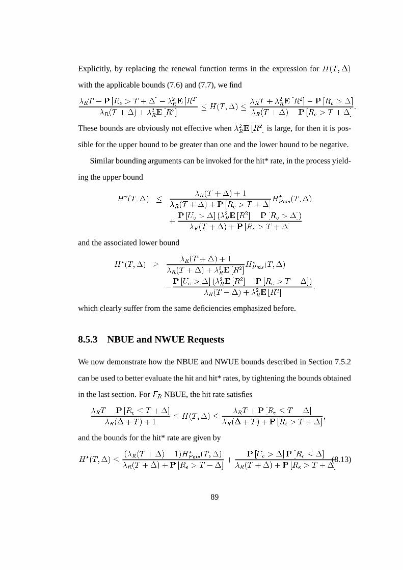
Explicitly, by replacing the renewal function terms in the expression for� ��#����!�
with the applicable bounds (7.6) and (7.7), we find� � # � � � ��� � #�� � � � � �
�� � � � �
� � ��#�� �!� � � ��� � � � � � � ��#����!� � � � #�� � �
�� � � � � � � � ��� �2� �
� � ��#�� �!� � � � ��� � #�� � � These bounds are obviously not effective when
� ��� � � � � is large, for then it is pos-
sible for the upper bound to be greater than one and the lower bound to be negative.
Similar bounding arguments can be invoked for the hit* rate, in the process yield-
ing the upper bound
� � ��#����!� �� � ��#�� �!� �(
� � ��#�� �!� � � � ��� � #�� � �� ���� � � ��#����!�
� � � � � ��� ��� � ��� � � � � � � � ��� �2� ���
� � ��#�� �!� � � � ��� � #�� � �and the associated lower bound
� � ��#����!� �� � ��#�� �!� �(
� � ��#�� �!� � � ��� � � � �
� ���� � � ��#����!�� � � � � �2� � � � �
�� � � � � � � � ��� � #�� � ���
� � ��# � �!� � � ��� � � � � �
which clearly suffer from the same deficiencies emphasized before.
8.5.3 NBUE and NWUE Requests
We now demonstrate how the NBUE and NWUE bounds described in Section 7.5.2
can be used to better evaluate the hit and hit* rates, by tightening the bounds obtained
in the last section. For� � NBUE, the hit rate satisfies
� � # � � � ��� ��# � � �� � � � � # � �( � � ��#����!� � � � #�� � � ��� �2#�� � �
� � � � � # � � � � � � � #�� � � �and the bounds for the hit* rate are given by
� � ��#����!� � � � � ��# � �!� �(/� � ���� � � ��#����!�� � ��#�� �!� � � � ��� � #�� � � �
� � � � �2� � � � ��� �,� �� � ��#�� �!� � � � ��� � #�� � �(8.13)
89

and
� � ��#����!��� � ���� � � ��#����!�� � � � � �2� � � � ��� �2#�� � �� � ��#�� �!� �( (8.14)
Similarly, with� � NWUE we have
� � # � � ��� � � � � �(
� � � � � # � � � ��� � � � � �
� ��#����!� � � � # � � ��� � � � � ��
� � � � � # � �( �
together with
� � ��#����!� � � ���� � � ��#����!� � � � � � ��� ��� � ��� � � � � ��/�
� � ��# � �!� �(and
� � ��#����!��� � � � ��#�� �!� �(/� � ���� � � ��#����!�� � ��#�� �!� � � �
�� � � � � � � � � � ��� ��� � �
�� � � � � ��/�
� � ��#�� �!� � � ��� � � � �
Although good bounds are already established for NBUE (and thus IFR) distri-
butions, the NWUE bounds are still not satisfactory, for the same reasons outlined
earlier. To further tune these bounds, we make use of Marshall’s linear bounds,
namely (7.16) and (7.17), in the expressions for the hit rate, and obtain� � # �(� � � � � �
� � � ��# � �!� � �
� � ��#����!� � � � #��)� � � � � �
� � � ��#�� �!� � � ��
Applying the linear bounds on the hit* rate yields
� � ��#����!��� � ���� � � ��#����!� � � � ��#�� �!� � � � ��#�� �!� � � ��� � � � � �2� � � � � � � �
� � � ��#�� �!� � � � (8.15)
and
� � ��#����!� � � ���� � � ��#����!� � � � ��#�� �!� � � � ��# � �!� � �
� � � � � ��� ��� � � � � � � � � ��# � �!� � �
(8.16)
The refined bounds are therefore achieved as we recall that� � � � (equivalently,
�
�)� ) whenever� � is NWUE (equivalently, NBUE), respectively.4
4See (7.18) and (7.19), as well as previously made comments in Section 7.5.3.
90
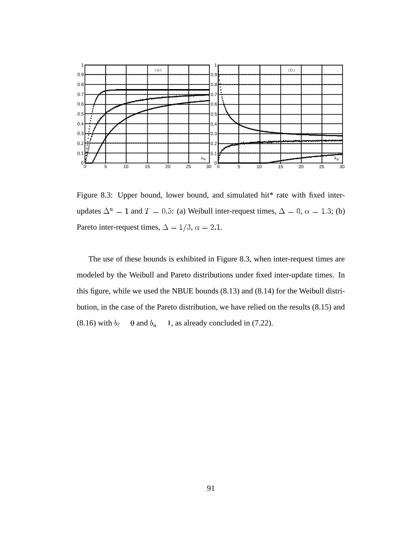
1
0.9
0.8
0.7
0.6
0.5
0.4
0.3
0.2
0.1
00 5 10 15 20 25 30
R
(a)1
0.9
0.8
0.7
0.6
0.5
0.4
0.3
0.2
0.1
00 5 10 15 20 25 30
R
(b)
Figure 8.3: Upper bound, lower bound, and simulated hit* rate with fixed inter-
updates �" !�5 and #3�%� '& : (a) Weibull inter-request times, � �$� , - �5� � ; (b)
Pareto inter-request times, �+�3/.�� , - �60� 1 .
The use of these bounds is exhibited in Figure 8.3, when inter-request times are
modeled by the Weibull and Pareto distributions under fixed inter-update times. In
this figure, while we used the NBUE bounds (8.13) and (8.14) for the Weibull distri-
bution, in the case of the Pareto distribution, we have relied on the results (8.15) and
(8.16) with� � �,� and
�
�� , as already concluded in (7.22).
91

92
Chapter 9
The Perfect TTL Algorithm
The perfect TTL is a non-causal consistency algorithm where the server knows at
any given time when the current version of�
will be updated. Each time the server
receives a request for�
, say at time � , it returns the current version together with the
residual lifetime value � ��� � � as its TTL. The downloaded document is placed in the
cache at time � � � , and is considered cache-fresh until � � � ��� � � .In general, Web servers are not capable of predicting the next master modification
time, therefore the implementation of the perfect TTL is not feasible in many caching
systems in practice. In spite of this fact, the perfect TTL algorithm can be easily
deployed in applications where the rollout schedule for the Web server is known in
advance, a common practice in commercial servers with frequently updated pages
[67].
The analysis of the perfect TTL is not only important for evaluating the consis-
tency performance that can be attained by the systems described in [67], but it also
contributes to understanding the limitations of other consistency protocols: Since the
93

perfect TTL is the single strong consistency algorithm in the class of TTL protocols,1
we expect this algorithm to produce the highest hit* rate among all TTL algorithms.
9.1 Rules of engagement
When � �+� , a document downloaded from the server in response to a cache-miss
at time # �� for some ��� ������ � � is instantenously placed in the cache, and the
server-fresh object is sent to the user. All requests that arrive during the time interval
��# �� � # �� � � ����# �� � � incur a hit and are served by the cache with a server-fresh doc-
ument. Consequently, each hit request produces a hit*, hence the perfect TTL is a
strong consistency algorithm. In addition, since the server-freshness of�
expires at
the precise moment of TTL expiration at time # �� � � ����# �� � , the server-freshness and
cache-freshness tracking processes are identical for all � � � , and the hit and hit*
rates are equal when � is indeed zero.
Now pick an arbitrary � �(� . The first miss request for�
arrives to the cache at
# �� �)� , the cache places the returned version at # �� � � , and forwards the downloaded
item to the user. If the master is updated prior to placement, i.e., � ����# �� � �3� , then
the cache immediately marks�
as invalid. On the other hand, if � ����# �� � � � , then
any subsequent request for�
at the cache in the time interval ��# �� � � � # �� � � ����# �� � �is served directly by the cache with a server-fresh copy.
As before, if a request at time # �� for some � �$�� 0��� � � is the first one presented
after the TTL has expired, then it is forwarded to the server. Requests presented
1See additional arguments below.
94

during the time interval ��# �� � # �� � �!� that find an invalid cached copy are forwarded
to the server as well. If a document returned from the server finds a zero TTL value
at the cache, then the TTL counter is reinitialized upon the placement of the newly
retrieved document.2
9.2 Quality of data under the perfect TTL
For the consistency algorithms considered in this dissertation, the cache-freshness
and server-freshness tracking processes, ��� � � � � � � � � � and ��� � � � � � � � � � � , re-
spectively, are related through � ��� � � � � � � � � � , for all � � � and � � � . These
two processes are obviously not equal in general, as previously demonstrated in the
analysis of the fixed TTL [8].
We have already established that if �5�6� , then under the perfect TTL the cache
and server freshness tracking processes coincide. This fact remains true even when
� is non-zero, as later explained in the hit* rate analysis in Section 9.4. The perfect
TTL is therefore a special case where � � � � � � � � � � � � for all � � � and � � � ,whence the hit and hit* rates are always equal. As a result, the QoD given by the
ratio (7.4) achieves its maximal value of one.
In spite of maximizing the QoD measure, it is erroneous to conclude that the
perfect TTL achieves a higher hit* rate than all other (including non-TTL) cache
2These operational constraints coincide with the rules of the fixed TTL algorithm discussed in
Section 8.1, where requests arriving after a cache miss at time ���� in the interval �������� ���� � � � for
� � � ���� , are also forwarded to the server. However, under the assumption � � � for the fixed
TTL, miss requests presented in this time interval never find a zero TTL upon their return to the cache,
hence do not affect the TTL of the cached copy.
95

consistency protocols: Consider the replication server-invalidation algorithm. Under
this algorithm, the server publishes master changes to the cache upon each update. As
a consequence, documents stored at the cache are always cache-fresh, therefore user
requests are always served by the cache. When �%�)� , master changes are replicated
to the cache instantenously, and every request is served with a cache-fresh* docu-
ment. In other words, when ���3� , the hit and hit* rates attained by the replication
algorithm are both equal to one, whereas under the perfect TTL the hit* rate (9.3) is
clearly less than one.
9.3 Zero delays
In the notation of the modeling framework, let ��� � � � � � � � � denote the cache
(and server) freshness tracking process of�
at the cache.3 This process has right-
continuous sample paths with left limits, and is defined by
� � � � �%� � ��#�� ��(� � � # �� � � � #
�� � ��� # �� ��
for each � �)������ � � , with the update rule
� ��#�� � �
������ ������ ����# �� � if � ��# �� � � �)�� ��# �� � � if � ��# �� � � ��� . (9.1)
The initial value of the process is taken to be � � � � � �)� so that � � � � � � ��� � � � � �by (9.1). The TTL expires at time � �)� if and only if � � � � ����� , and therefore the
�� request at time # �� produces both a hit and hit* if and only if � ��# �� � � �2� .
3Since ������� $ � � $ � �� ����� � � $ � � $�� �� for � � from previous arguments, we only refer
to the process ������� $ � � $ � �� throughout this chapter. Furthermore, in this section � � and is
omitted from the notation.
96

The tracking process ��� � � � � � � � � is related to the residual lifetime process
� � ��� � � � � � � � , but is not identical to it. To appreciate this fact, introduce the
sequence ��� � � � �)������ � � � of � -valued rvs through
� � � ����� ��� �)������ � � � # � �2#�� � (9.2)
As the rv � � identifies the first request made after the � � update, � � ������ � � ,the rv # ���� represents the first request epoch after that update taking place at # � . It
is easy to check that the two processes coincide everywhere except in each interval
� #� � � # ���� � where the tracking process vanishes. In particular, � ��# ���� � � � � and
the request occuring at time # ���� incurs a miss. However, all the requests made in
the interval ��# ���� � # ���� � � ����# ���� � � result in a hit. This fact allows for an equivalent
definition for the TTL tracking process, namely
� � � � � � � ��# ���� ��(� � � # ���� � � whenever # ���� � ��� # ���� �� for each � �,������ � � , with the update rule
� ��#���� � � � ����# ���� �
We use the initial condition � � � � � �)� so that � ��# �� � � �,� � � � � � � .The corresponding hit rate
�(and thus the hit* rate
� � as well) is defined at (7.2)
with ��� � � � � ���(� � .
Proposition 9.1 If the point processes ��# �� � � �������� � � � and ��# � � � �������� � � �are renewal processes, the common value of the hit and hit* rates is given by
� � � � �� � � � ��� ������ � � � � � � (9.3)
97

The proof of this proposition is omitted as it is available by assigning � � � in
Proposition 9.2.
In the expression (9.3) the stationary forward recurrence time � � is taken to be
independent of the counting process � �4� � � � � �+� � , and its distribution is given by
(7.5). An alternative expression for�
can therefore be written as
� � � � �� � ��
� � � � �3��� � � � �3��� � �� (9.4)
and is a direct consequence of (9.6) with �+�,� .
9.4 Non-zero delays
A request presented at time # ���� finds an invalid cached document and incurs a miss.
The downloaded copy is placed in the cache at # ���� �!� and expires at # ���� � � ����# ���� � ,possibly prior to placement. All requests that arrive in the interval ��# ���� � # ���� �(�!�also find an expired cached copy and are forwarded to the server as well, to increase
the consistency of�
at the cache: If # ���� � #� � �� � # ���� � � for some � �)������ � � ��then the document placed at time # ���� ��� is immediately stale, and requests made
during � #� � �� � # ���� � �!� retrieve the latest version of�
and replace the stale replica.
These dynamics are illustrated in Figure 9.1.
Under these rules of engagement, the validator tracking process ��� � � � � � � � � �can be defined as
� � � � � �$� � ����#�� � �!� �(� � �(��# �� � �!� � �
98

Server updates
h - hit & hit* m - miss
tCache requests
Ue(t)
L(t),L*(t)
hhhm m m mm
Figure 9.1: Time line diagram of requests, updates, and the tracking process of the
perfect TTL algorithm for ����� .
whenever # �� � � � ��� # �� �� � � , and adopts the update rule
� � ��#�� � �!� �
������ ������ � ����# �� �� �!� if � � � ��# �� � �!� � � �)�� ��� ��# �� � �!� � � if � � � ��# �� � �!� � � ���
This tracking process can again be related to the residual lifetime process � � ��� � � � ���� � as follows: If # ���� �3� � #� � �� (equivalently, � ����# ���� � � � � � ) for some
� � ������ � � , then the two processes coincide on each interval # ���� ��� � � �# � �� , whereas ����� � � � � in each interval � # � � # ���� ���!� . In all other cases where
# ���� �,� � #� � �� , the tracking process is zero in the interval � # � � #� � �� � . In other
words, the two processes coincide wherever the tracking process is non-zero. These
observations lead to the alternative definition of the tracking process given by
� � � � � �%� � � ��#���� � �!� �(� � �(��# ���� � �!� � �
99

on each time interval # ���� � � � ��� # �� � � � � � �� �)������ � � , updated by the rule
� � ��#���� � �!� �%� � ����# ���� �� �!� �
with the initial value ��� � � � � � at � �,� . Moreover, by the fact that ��� � � � � � ��� � �on the set � ���(� � � ��� � � ��� � it is plain that each hit request incurs a hit*, whence
the processes ����� � � � � � � � � and ��� � � � � � � � � � � coincide, as in the case of zero
delays.
The hit rate� � �!� is given in (7.2) with the tracking process ��� � � � � � ���(� � , and
an expression for it is available in the following proposition.
Proposition 9.2 With the assumptions of Proposition 9.1, the common value of the
hit and hit* rates is given by
� � �!� � � � � �!� � � � � � � ��� � ��� � � ��� � � �� � � � � ��� (9.5)
� � � � � � ��� � ��� ��� � � � � �� � � � � ���
� � � ��� � � � � � � � � � � � �!� ���� � � � � � �
As expected, when � �6� this result specializes to the one stated in Proposition 9.1.
A proof of Proposition 9.2 is available in Appendix C.
Here again, the rv ��� in (9.5) is taken to be independent of the counting process
� �4� � � � ���(� � . This fact allows us to rewrite the hit rate as
� � �!� � � ��
� �
� � � � � � � � � � ��� � ��� ��� � � ��� � � �� � � ��� � (9.6)
�6� � � � � � �!� ����� ��
� � � � ��� ��� � � � � �3� � � �/�
which reduces to (9.4) for ����� . A proof of the alternative expression (9.6) is also
provided in Appendix C.
100
9.5 Bounds and properties
Bounds on the hit rate produced by the perfect TTL can be derived from the expres-
sion (9.5), for any inter-request time and inter-update time distributions. Explicitly,
under the renewal assumption on the point process of requests, we have4� � � � � � ��� � � � � � � � �� � � � � � � � � � � � ��� � � � � � � � � � �!� � �
� � � � � ��� � (9.7)
and we obtain the lower bound
� � �!��� � � � � � � �!� �� � � � � ��� (9.8)
An upper bound can be developed by removing the negative term in the left hand side
of the expression (9.7) for the hit rate. This yields
� � �!� � � � � ��� � � � � � � � � � � � �!� ���� � � � � ��� � (9.9)
and equality is achieved whenever �+�)� .The single parameter that affects the consistency performance of the perfect TTL
is the download delay � . Under the operational rules of this algorithm, we (in-
tuitively) anticipate that increased communication delays would degrade the cache
consistency outcome. This is indeed the case, as concluded in the following proposi-
tion.
Proposition 9.3 The hit rate produced by the perfect TTL algorithm is a non-increasing
function of � , with ����� ��
� � �!� �,� .
Proof. Take � � �+� � �%� . From the expression (9.6) for the hit rate, it is simple
4A proof for (9.7) is provided in Appendix C.
101
matter to check that
�
�� � � � � �� � � � � � �
�� �
� ���
� �� � � � � ���/� � ��� � ��� � ��� � � � � ��� �
� � � � � � � � � � ���� �
� � � � � �� � ��� � � � ��� � � �� � � ��� �
��� � � � � � � � � � � � � � � � � ���� � � � ��� ��� � � � � � �3� � � �/
The desired result� � � � � � � � � � ���(� follows by replacing
� � � ���/� � with� � � � � � � �
(clearly not greater than� � � ���/� � for � in the interval � � ����� � � ), cancelling the first
two terms in this last expression, and recalling that� � � � � � � � � � � � � � � � � �(� .
The asymptotic behavior of� � �!� can be derived from (9.6) as well: First, the
hit rate can be rewritten as
� � �!� � � ��
� �
� �
� � � � � � � � � � ��� � ��� ��� � ��� � ��� � � ��� �
�6� � � � � � �!� ����� ��
� � � � ��� ��� � � � � �3� � � �/
Letting � go to infinity, we find
����� ��
��
� �
� �
� � � � � � � � � � ��� � ��� ��� � ��� � ���� � � ��� � � ��
� � � � � � ��� � �3�
This result is a simple consequence of the Renewal Equation [69] according to which
� � � � � � �� � �
� � � � �� ��� � � � ��� � ��� � ���(�
Then, by applying the Basic Renewal Theorem (8.10) and recalling ���� �� � � � �3� � � �)�
(implied by the integrability of�
� ), we have
����� �� � �
� � � � �!� ����� ��
� � � � ��� ��� � � � � �3� � � �
102

� ����� ��
� � ��
� � � � � ��� ��� � � � � �3� � � �
� ����� ��
� � ��
� � � � � ���2� � � � ��� � � �
� ��
which completes the proof of the proposition.
9.6 Evaluation of the hit and hit* rates
9.6.1 Poisson requests
When inter-request times are exponentially distributed with rate� � , the hit rate of
the perfect TTL can be written as
����� � ��� �!� � ��� �� � � �!� � � � �� �
��� ����� � � � � � � �
��
� ������ � � � � � � �!� � � � (9.10)
with mapping� ��� � � � � given by
� ��� � ��� �,� ��� �� � �� �(�
This mapping is monotone increasing, thereby confirming the validity of Proposition
9.3 for the special case of Poisson requests.
A closed form expression for the hit rate can be found in some scenarios. For
instance, under periodic updates where�
is altered every �! time units, we find that
����� � ��� �!� �)�� � �(� �
103

1
0.9
0.8
0.7
0.6
0.5
0.4
0.3
0.2
0.1
00 5 10 15 20 25 30
R
= 0.5
= 0
= 0.2
= 1/3
= 0.1
Figure 9.2: The hit and hit* rate of the perfect TTL with Poisson requests and fixed
inter-updates �4 *�3 , for several values of � .
while with �" "��� the expression (9.10) becomes
����� � ��� �!� � �" � �� � � � � � ��� �����
� ��� � � � This hit rate is presented in Figure 9.2 for several values of the delay � , where we
can now visualize the degradation of the hit rate as � increases.
9.6.2 Distribution-free results
The bounds presented in (9.8) and (9.9) are not very useful in general applications, as
the value of the renewal function� � � � � � � may not be known in closed form for every
���(� . To circumvent this difficulty, additional bounds can be derived by utilizing the
bounds on the renewal function discussed in Chapter 7.
A new upper bound can be developed by replacing the term� � � � �!� � in the upper
104
bound expression (9.9) with the lower bound (7.7), so that
� � �!� � � ��
� � � � ��� � � � ����� � � � � � � ��� ��� ��� (9.11)
In this last term we have taken� � � � � � � � � � � � � �
� , by virtue of the fact that the rv
� is independent of the stationary point process of user requests.
A lower bound on the hit rate can be derived in a similar manner, by assigning
(7.6) in the lower bound (9.8). This action results in a smaller lower bound than the
one reported in (9.8), which is given by the expression
� � �!��� � ��
� � �� � � � � �
���� � � � � (9.12)
The new lower bound is inefficient when� ��� � � � � is large, and therefore better
bounds are still required.
To conclude this section, note that additional bounds can be obtained by using the
Marshall bounds. Replacing the term� � � � �!� � with the corresponding lower bound
(7.17) in the upper bound expression (9.9) yields
� � �!� �� � ��
� � � � ��� � � � ����� � � � � � � � � (9.13)
Similar calculations provide us with the lower bound
� � �!��� � ��
� � � � � � � � �
� � (9.14)
with� �
and�
given in (7.14) and (7.15), respectively.
9.6.3 NBUE and NWUE Requests
The hit rate under the perfect TTL algorithm can be better estimated by tightening
the bounds listed thus far. This goal is achieved in this section when the distribution� � is either NBUE or NWUE.
105

1
0.9
0.8
0.7
0.6
0.5
0.4
0.3
0.2
0.1
00 5 10 15 20 25 30
R
1
0.9
0.8
0.7
0.6
0.5
0.4
0.3
0.2
0.1
00 5 10 15 20 25 30
R
(a) (b)
Figure 9.3: Upper bound, lower bound, and hit rate simulation results under fixed
inter-update times �4 = 1: (a) Weibull inter-request times, � � � '0 , - � � � ; (b)
Pareto inter-request times, �+�3/.�� , - �60� 1 .
If the inter-request time distribution is NBUE, the previous lower bounds can be
revisited to write
� � �!��� � ��
� � � � � � �!�
as we recall that�
� � in (9.14) for all NBUE distributions. Combining this last
inequality with (9.11) we find that the distance between the upper and lower bounds
for NBUE inter-request time distributions is given by
��
� � ��� �� � �!� � � ��� � ������� � � � ��� � � � � � � � ��� �(� � � �
so that the hit rate can already be well-estimated when � is small and� � �*� �
� , as
is the case in most Web applications.
Similarly, if� � is NWUE, then the bound
� � �!� � � ��
� � � � ��� � � � ����� � � � �!� (9.15)
106

follows from (9.13), since now� � � � . Here, the lower bound (9.12) that suffers
from the disadvantages mentioned earlier remains the best lower bound for general
NWUE distributions. However, once the distribution� � is given, improved bounds
can still be derived. For example, when� � is the Pareto distribution, then
�
� ,and the lower bound (9.14) is given by
� � �!���� � ��
� � � 0�� � � �!�
These bounds, together with the NBUE bounds, are illustrated in Figure 9.3 for the
Pareto and Weibull inter-request time distributions, respectively.
107

108

Part III
Proofs
109


Appendix A
A Proof of Theorem 4.1
Theorem 4.1 is a direct consequence of the following fact:
Proposition A.1 For each #(�)������ � � �� it holds that
����� ��� � � � � � � ��� � � � � � � � � � �*� � � (A.1)
� ����� ��� � � � � � � � � ��� � ����� � �for any � � ����� in
�with � not in � .
Equality (A.1) is understood to mean that� � � � � � � � � � � � � � � ��� �� � � � � � � � � � � � � � � � (A.2)
holds with � given by
� � ����� ��� ��� � � � � � � ���� ������ � (A.3)
The proof proceeds by induction on #,�,������ � � .The basic step - Fix � � ����� in
�and note that
� � � � ����� � � � � � � � ��� ��� (A.4)
111

Thus, for � in � � � distinct from � (also in � � � by virtue of its definition (A.3)),
we have � � � � � � � � � � � � � � �� � � � � � � � � � � � � � ��� � � � �� � � � � � � � � � � � ��� � � � � � � � � � � � �� � ��� � � � �
with a similar expression for� � � � � � � � � � � � � � � . Hence,� � � � � � � � � � � � � � � � � � � � � � � � � � � � � � �
� � ��� � ����� ��� � � � � ��� � � (A.5)
and (A.1) does hold for #,�,� .The induction step - Assume (A.1) to hold for some #(�6������ � � . Fix � � ����� in
�with � not in � . We need to show that for � in � � � , we have� � � � � � � � � � � � �� � � � � � � � � � � � � �(� (A.6)
with � given by (A.3).
Fix � in � � � and note that � � �
is distributed like � �
and is independent of it, by
the IRM. Using the DPE (4.3) we can write� � � �� � � � � � � � � � � �� � � � � � � � � � � � � � � � � � � � � � � � � � �� � � � � � � � � � � � � � ��� � � � � (A.7)
� � �� � � � � � � � � � � ���
� �� � � ��� � � � � � � � � � � � � � � � � � � � � ���* Note that
� � � � � � � � � � � � � � � � � � � � � � � � � �
112

� � � � � � � � � �,��� � � � � � � � � � � � � � � � � � � �� � � � � � � � � � � � � � � � � � � � (A.8)
with � defined by (A.3), and that� � � � � � � � � � � � � ��� � � � �� � � � � � � � � � � � ��� � � � � � � ��� � ����� � (A.9)
Finally, � �� � � � � � � � � � � ���
� �� � � ��� � � � � � � � � � � � � � � � � � � � � ���� � �
� � � � � � � � � ��� � �� � � ��� � � � � � � � � � � � � � � � � � � � � ���
� � ��� � ��� � �� � � � � � � � � � � � � � � � � �� (A.10)
Reporting (A.8), (A.9) and (A.10) into (A.7), we conclude that� � � �� � � � � � � � � � � ���� � � � � � � � �,��� � � � � � � � � � � � � � � � � � � �� � � � � � � � � � � � ��� � � � �� � ��� � ����� � � � ��� � ���
� �� � � � � � � � � � � � � � � � � �� � � � � � � � � � � � � � � � � � � � (A.11)
� � �� � � � � � � � � ���
� �� � � ��� � � � � � � � � � � � � � � � � � � � � ���* We can now write the corresponding expression (A.11) with � replaced by � , and
the difference in (A.6) takes the form� � � �� � � � � � � � � � �� � �� � � � � � � � � � � ���� ��� � ����� � � � � � � ��� � �
��� � � � � � � � �(��� � � � �/� � � � ��� � � � � � � � � � � � ��� (A.12)
113

with
� � � � � � � � � � � � � � � � � � � � � � � � � � � � � � � � � � �� � � � ���
� �� � � � � � � � � � � � � � � � � � � � � � � � � � � � � � � � � �� � � � � � � � � � � � � � � � � � � � ���
� � �� � � � � � � � � � � � � � � � � � (A.13)
and
��� � � �� � � � � � � � � ���
� �� � � ��� � � � � � � � � � � � � � � � � � � � � � �� � �
� � � � � � � � � ���� � �� � � � ��� � � � � � � � � � � � � � � � � � � � � � �
Observe that � ��� � ����� � � � � � � ��� � ���(� by the definition of � and that the condition
� ���,� , being equivalent to (A.1), holds true under the induction hypothesis. Again,
by invoking the hypothesis we have that
��� � �� � � � � � � � � � � � � � � � � � � � � � � � � � � � � � � � � �
and therefore concludes � � �,� . Similarly, for � � we get� � � � � � � � � � � � � � � � ��� � �� � � � � � � � � � � � � � � � � �
� � � � � � � � � � � � � � � � � � � � � � � � � � � � � � � � �)� � �which is non-negative as argued earlier in the context of � � .
Consequently, it is already the case that� � � �� � � � � � � � � � �� � �� � � � � � � � � � � � �,� (A.14)
directly from the induction hypothesis, and (A.3)-(A.6) will hold if we can show that
��� �,� . Inspection of � � reveals that � � �,� provided
��� � �� � � ��� � � � � � � � � � � � � � � � � � � � � �� ���
� � �� � � � ��� � � � � � � � � � � � � � � � � � � � � � �(� (A.15)
114

whenever � �
is not in � � � .To establish (A.15) we find it useful to order the set of documents � ��� � � � � �
according to their expected cost: For � and � in � ��� � � � � � we write � � � (re-
spectively, � � � ) if � ��� � ����� � ��� � � � ��� � � (respectively, � � � � ��� � ��� � ��� � ����� � ), with
equality � � � if � ��� � ����� � ��� � � � ��� � � . With this terminology we can now interpret �
as the smallest element in ��� � according to this order. Two cases emerge, depending
on whether � � � �
or � �
� � :
Case 1 - Assume that � �
� � with � �
not in � � � . Then, consider
��� � �� � � ��� � � � � � � � � � � � � � � � � � � � � � (A.16)
and note that � �
is not in � � � � � and that � �
is the smallest element in � � � � � �
(thus in � � � � � � which contains it). By the induction hypothesis applied in the
state � � � � � � � � � � , the minimization (A.16) is achieved by the selection � � ��� �
,
so that
��� � �� � � ��� � � � � � � � � � � � � � � � � � � � � � � � � � � � � � � � � � � � � ��
The same argument shows that
���� � �� � � � ��� � � � � � � � � � � � � � � � � � � � � � � � � � � � � � � � � � � � � �
by applying the hypothesis on the state � � � � � � � � � � . Combining these facts, we
get
��� � �� � � ��� � � � � � � � � � � � � � � � � � � � � �� ���
� � �� � � � ��� � � � � � � � � � � � � � � � � � � � � �� � � � � � � � � � � � � � � � � � � � � � � � � � � � � � � � (A.17)
115

and (A.15) follows by invoking the induction hypothesis once more, this time in state
� � ����� .Case 2 - Assume � � � �
with � �
not in � � � . Then, going back to the expression
(A.16), by virtue of the induction hypothesis applied to the state � � � � � � � � � � , we
find that
��� � �� � � ��� � � � � � � � � � � � � � � � � � � � � �
� � � � � � � � � � � � � � � � � � � � �
and (A.15) now follows by invoking the induction hypothesis once more, this time
in state � � � � � � � � � � , as we note that any element � � in � ��� with � ��� � is
necessarily in � � � � � , hence in � � � � � � � �
. This completes the proof of
Theorem 4.1.
116

Appendix B
Proofs of Propositions 8.3 and 8.4
In the next sections B.1 and B.2, we make use of the � -valued rvs � � ��� �!�)������ � � �defined recursively through (8.5). Note that � ��# ���� �*� � � for all � �������� � � , and
that under the renewal assumptions on the request process, the rvs � � ��# �� � � � � �� ��# �� � � � � � ������ � � � are i.i.d., each distributed according to � ��# �� � � . Therefore,
by the Strong Law of Large Numbers we find
����� �� � �� � ����� ��
�
� � ��� � �
�� ��#
�� � � � �� � ��#
�� � ��� ��� � ��# �� � �
� � ��� (B.1)
By the very definition of # �� � , we have that��� � ��# �� � �� �� � � � � � ��#�� �!� � � ��� (B.2)
as explained through arguments below.
B.1 A proof of Proposition 8.3
Since the rvs � � ��� �!�)������ � � � monotonically exhaust � a.s., it is plain that
� ��#����!� � ����� �� � �
����� ��� � � � � ��#
�� � � ��� � � ���
117

In order to make use of this fact, fix � � ������ � � and consider the dynamics of the
freshness tracking process on the interval ��# ���� � # ���� � � � : With # ���� � � ��# ���� � � , we
have � � � � � � �%� since � � ��# ���� � �%� . The validator process is reinitialized at time
# ���� � � to the value ������# ���� � �!� �,# , returning to zero with the expiration of the
TTL at time # ���� � � � # , i.e., � � � ��# ���� � � � # � � � �)� .Thus, the requests made at the cache in the interval ��# ���� � # ���� � � � incur misses,
while those occurring in ��# ���� � � � # ���� � � � # � are necessarily hits. Also, there is
exactly one request made in the interval � # ���� � � � #�� # ���� � � � , and it is necessarily a
miss. In summary, we see that there are exactly � � � ��# ���� � �!� � � ��# ���� � � misses
in the interval ��# ���� � # ���� � � � . Therefore, for each �!���� 0��� � � , we get
����� ��� � � � � ��#
�� � � �,� ��� � � ��
� � ��
� ������� � � � � �� � ����#
�� � � �,� �
�� � ��� � � � � � � ��# �� � � �!�� � ��# �� � � � � (B.3)
Again, under the renewal assumption on the request process, the rvs � � ��# �� � � �!���� ��# �� � � � � � ������ � � � are i.i.d. rvs, each distributed according to � � �!� , and the
Strong Law of Large Numbers now gives
����� �� �
� � ��� � � � � ��#
���� � �!�� � ��# ���� ��� � � � � � �!� � � ��� (B.4)
Since
� � ��#����!� � ����� �� � �
����� ��� � � � � ��#
�� � � �,� ��� ��� 1�
it is plain from (B.3) and (B.4) that
� � ��#����!� � � � � � � �!� � � � � � � ��# � �!� � � �
118

by the usual arguments, as we recall (B.1) with (B.2). The desired expression (8.6)
is finally obtained.
B.2 A proof of Proposition 8.4
The arguments are similar to those given in the proof of Proposition 8.3. We begin
by noting that
� � ��#����!� � ����� �� � �
����� ��� � � � �
� ��#�� � � �2� ��� ��� (B.5)
In order to use (B.5), fix � �)������ � � and consider the cache-fresh* tracking process
on the interval ��# ���� � # ���� � � � : A download is requested at time # ���� , resulting in a cache
placement at time # ���� � � . If no update occurs before this cache placement, then the
validation process is reinitialized at time # ���� � � to the value ��� ��#���� ����# ���� � � �!� ,and returns to zero with the expiration of this TTL. In other words, � �
� � ��#���� � � �
��� ��#���� ����# ���� � �,�!� � � �!� � . On the other hand, if an update occurs before the
placement, i.e., � ����# ���� � �(� ,1 then � �
� � � � �)� on the entire interval ��# ���� � � � # ���� � � � .As already discussed in the proof of Proposition 8.3, the hits on the interval
��# ���� � # ���� � � � can occur only in the subinterval ��# ���� � � � # ���� � � � # � . If � ����# ���� � �(� ,
none of these requests can be hits*. However, if � � � ����# ���� � , then all the requests
made in the interval ��# ���� � � � # ���� � ��� � � � #���� ����# ���� � � � are hits*, while none of
those made in the interval � # ���� � ��� � � � #���� ����# ���� � � � # ���� � � � #�� are as they are
all hit but miss* requests. Summarizing, we conclude that the number� �
� of hits* in
1Only applies when � � .
119

the interval ��# ���� � # ���� � � � is given by the difference
� �
� � � � ��#���� �� ��� � � � #���� ����# ���� � � � � � � � ��# ���� �� ��� � � ��� ����# ���� � � �
Consequently, for each �!�,������ � � , we can write����� ��� � � � �
� ��#�� � � ��� � � � � ��
� � ��
� � ����� � � � � �� � �
� ��#�� � � ��� � � � � ��
� � �� �� (B.6)
Under the renewal assumptions on the independent processes ��# �� � � �)������ � � � and
��#� � � � �)������ � � � , we can easily verify the following: First, we have the equalities
����� �� �
� � ��� � � � � � ��#
�� � �� ��� � � � #���� ����# �� � � � � � �� � ��# �� � ���
� � � � � ��� � � � #���� � � � � � � ��� 1�and
����� �� �
� � ��� � � � � ��#
�� � �� ��� � � ��� ����# �� � � � �� � ��# �� � � � � � � � � ��� � � ��� � � � � � ���
In both cases the rv � � is taken to be independent of the counting process � � � � � � ���� � . Combining, we get
����� �� �
� � ��� � �
� �� � � � � � ��� � � � #���� � � � � � � � � � � ��� � � ��� � � � � � ��� (B.7)
To conclude, we report (B.6) and (B.7) into (B.5), and this yields
� � ��#����!� � � � � � ��� � � � #���� � � � � � � � � � � ��� � � ��� � � � � � � � � � ��#�� �!� � � �
as we recall (B.1) with (B.2).
In order to derive the alternative expression (8.8) we expand the expression (8.7),
and by taking the rv � � to be independent of the point process of requests we get
� � ��#����!� � � � � ���2#�� � � � � � ��# � �!� � � � � � � �2� � � � � � �!� �� � � ��#�� �!� � �(�
� � � � � ��� � ��# � � � � � � ��� �� � � ��#�� �!� � �(
120

Then, simple manipulations of this last term lead to� � � � � � � � �2#�� � � � � � � � � � ��
� �� �
� � � ��� � � � � �3� � � �
and the desired result (8.8) follows from the fact that
� � � ����# � � � � � � ��#�� �!� � � � � � � �2� � � � � � �!� �� � � ��#�� �!� � �(� � � � � � #�� � � � ��#����!�� � � � � � � �2#�� � � � � � � �!� �� � � ��#�� �!� � �(� � � � � ��� � � ��#����!�� � � � � � � �2#�� � � � � � ��#�� �!� �� � � ��# � �!� � �( �
as we recall that � � is distributed according to (8.3).
121

122

Appendix C
A Proof of Proposition 9.2
Throughout this proof we shall make use of the � -valued rvs ��� � � � � ������ � � �defined recursively through (9.2). In addition, we find it useful to introduce the se-
quence of � -valued rvs � � ��� �!�)������ � � � defined through
� � � ����� � � �)������ � � � # � �2#�� � � � (C.1)
so that # � � identifies the most recent document update time taking place prior to
the request at time # �� � . With (C.1), the requests and updates processes are related
through
#�� � ��# � � � ������# � � � � (C.2)
or alternatively via
# � � �� ��# � � � � � � �� �(# �� � � � ����# �� � � � (C.3)
for each �!�)������ � � .Since the rvs ��� � � � �)������ � � � monotonically exhaust � a.s., it is plain that
� � �!� �� ������� ��
� �
����� ��� � � � � ��#
�� � � �,� � � ��� (C.4)
123

In order to make use of (C.4), fix � � ������ � � and consider the dynamics of the
freshness tracking process on the interval � # ���� � # �� � � � � : If # ���� �6� � # �� � � � , the
miss requests in this interval1 are those that arrive to the cache during � # ���� � # ���� �� ����# ���� � � , as we recall that the request at time # �� � � � is the first one presented after
the update at time # ���� � � ����# ���� ���3#� � � �� . In fact, there are exactly � � ��# ���� �� ����# ���� � � � � ��# ���� � such requests. On the other hand, when # ���� � � �2# �� � � � , miss
requests are those presented in the time interval � # ���� � # ���� � �!� , and there are exactly
� � ��# ���� � �!� � � ��# ���� � such requests. To summarize, denote by � � the number
of miss occurrences on each interval � # ���� � # �� � � � � , therefore
� � � � � ��# ���� �� ��� � � ��� ����# ���� � � �� � ��# ���� � Combining all facts and observations, we get that for each � �6������ � � , it holds
that����� ��� � � � � ��#
�� � � �,� � �
� � ��� � �
�� ������� � � � � �
� � ����#�� � � �)� � �
� � ��� � � �
�
Now, the processes ��# �� ���2�������� � � � and ��#� � � � �������� � � � are assumed mu-
tually independent renewal processes, and by the Strong Law of Large Numbers we
can write
����� ��
�
� � ��� � � �
� �3 � ��� � � ��� � � ��� ����# �� � � � � � � ��� (C.5)
By the fact that the processes � � � ����� � � � � � � � � � � and � � � � � � � � � � � are
stochastically equivalent, an alternative expression for (C.5) is given by2
����� ��
�
� � ��� � � �
� � ��� � � ������# � � � �� ��� � � ��� ����# �� � � � � � � ���
1This only applies when � � .2Here, we make use of the fact that ������ � , which follows directly from the modeling framework;
see Section 7.1.1 and Section 7.1.2 for details.
124

Applying the relationships (C.2) and (C.3) in this last result we conclude that
� � � �� � ������# � � � � � ����# �� � � � � �)������ � � ��
and the result (C.5) can again be rewritten to yield
����� ��
�
� � ��� � � �
� � � � � � ��� � ������# � � � � � ��� � � � � ���
Next, it is simple to check that� � � � ��� � ������# � � � � � ��� � � �� ���
�� � � ������# � � � � � � � � � � �
� � ��� � � ������# � � � � � � � � ������# � � � � �!� � (C.6)
By the fact that
� � ������# � � � � �!� �3 � �� � � �
� ��� � � � � �(� � �3 � � � �!�
we get that the rvs � � ������#� � � ��� �!� and �� � � ������#� � � � � � � are independent. This
holds true since ������#� � � � depends on the rv � � , which under the renewal assumption
on the process of requests is independent of the rvs � ��� � ��0������ � � . Then, (C.6)
becomes ��� � � ��� � ������# � � � � � ��� � � �� ���
�� � � ������# � � � � � � � � � � �
� � � � � ������# � � � � � � � � � � � � �!� ��� � (C.7)
and we replace ������#� � � � with ��� as we recall that the two rvs are identically dis-
tributed.
125

To complete the proof, it is left to calculate ���� � �� ���� . In order to do so, we
must first define the delayed renewal process associated with the requests: Consider
the point process ��# ��� ����� ������ � � � with the understanding that the � � request
occurs at time # ��� , and # ��� � #� � � � � . Thus, # ��� ��# ��� �� for each �6� ������ � � .Let �
�� � ������2�������� � � � denote the sequence of inter-request times with
�� � �� �
# ��� �� � # ��� for each �2�5����� 0��� � � . This point process is assumed to be a renewal
process, and it is related to the point process of requests defined in Section 7.1.1 as
follows: ��� � �� ��� �3�� 0��� � � � form a sequence of i.i.d rvs, each distributed according
to the common cdf� � ; the rv
�� ��� ������#� � � is distributed according to the cdf
� ��� ,
and�� � � �� � ������ �3�� 0��� � � are mutually independent rvs.
The counting process ��� � � � � � ��� � associated with the point process ��# ��� ��� �
������ � � � is given by
��!� � � � ����� ��� �)������ � � � # ��� � � � � ���(� (C.8)
so that�� � � � counts the number of requests in the interval � �� � � . Here, ��# ��� ���+�
������ � � � is a delayed renewal process, therefore there exists a rate� � that satisfies
� � � ����� �� �� � � �� � ���
In this case, the Renewal Function is known in closed form [69], and is given by� � �� � � � � � � � � ���(� (C.9)
To finalize the proof, we have
����� �� � �
�� ����
� �� �
� � ��� � � � � ��#
� �� � � � � ��# � ���� ����
� �� �
� � ��� � � � � � ��#
� � � � �� � � �� � ��# � � �
126

� � � �� � � � � � ���
� � � � � � ��� � ��� � � � � � �
� � ��� (C.10)
By substituting (C.7) into (C.5), and applying the results (C.5) and (C.10) in the hit
rate definition (C.4), we obtain the desired result (9.5).
We conclude this appendix with the derivation of the alternate expression (9.6)
and the inequality (9.7). First, observe that � � � � can be expressed as
� � � � � � � ����� � � ����� � �� � � �
������ � � �
��� � � � � � � �
Under the enforced assumptions on the point processes of user requests and document
updates (see Section 7.1.1 and Section 7.1.2, respectively), we have the identification
#� � � �,� . We can therefore write the first term in (C.7) as� � � � � � ����� � � � � � � � � � ��� � � � � � ��� � ����� � � ��� ���� � � �
� � � �� ��� � � � � � � � ����� � � ��� � � �
and under the renewal assumption on the request process this expression becomes� � � � � � ����� � � � � � � � � � �� � �
� �
� � � � � � � � � � ��� � ��� ����� � �3� � � �� � � ��� �
By applying similar arguments on the second term in (C.7), we find that
� � � � ����� � � � � ��� � �� �
� � � � �� � � �3� � � ���
� � �� �
� � � � �3� ��� � � � � �3� � � � �
� � �� � � � �3� ��� � � � � �3� � � �/�
127

and the expression (9.6) for the hit rate follows by reporting the last two results into
(9.5), and replacing the denominator with (C.10).
It is now left to prove the upper bound (9.7). Since the counting process � � � � � � ���� � is non-decreasing in � , we have that� � � � � � ����� � � � � � � � � � � � � � � � � � ����� � � � � � � � ����� � � � �!� � Under the renewal assumption on the point process of requests, the rv � � � ��� � ��� �!�and the rv � � � �!� are identically distributed. Using the fact that the rv � � � ��� � � � �!�is independent of ����� � � (shown earlier in this appendix), we get� � � � � � ����� � � � � � � � � � � � � � � � ����� � � � � � � �' � � � �!� � �
which leads directly to (9.7).
128
Bibliography
[1] S. V. Adve, Designing Memory Consistency Models For Shared-Memory Mul-
tiprocessors, Ph.D. Thesis, Department of Computer Sciences, University of
Wisconsin-Madison, Madison (WI), 1993.
[2] A. Aho, P. Denning and D. Ullman, “Principles of optimal page peplacement,”
Journal of the ACM, Vol.18, no. 1, January 1971.
[3] V. Almeida, A. Bestavros, M. Crovella and A. Oliveira, “Characterizing refer-
ence locality in the WWW,” In Proceedings of the 4th International Conference
on Parallel and Distributed Information Systems (PDIS), pp. 92-107, 1996.
[4] M. Arlitt, L. Cherkasova, J. Dilley, R. Friedrich and T. Jin, “Evaluating content
management techniques for Web proxy caches,” In ACM Performance Evalua-
tion Review, Vol. 27, no. 4, pp. 3–11, March 2000.
[5] S. Asmussen and M. Bladt, “Renewal theory and queueing algorithms for
matrix-exponential distributions,” in: Matrix-Analytic Methods in Stochastic
Models, S. R. Chakravarthy and A. A. Alfa, Eds., Marcel Dekker, New-York
(NY), 1996.
129

[6] O. I. Aven, E. G. Coffman and Y. A. Kogan, Stochastic Analysis of Computer
Storage, D. Reidel Publishing Company, Dordrecht (Holland), 1987.
[7] O. Bahat and A. M. Makowski, “Optimal replacement policies for non-uniform
cache objects with optional eviction,” In Proceedings of INFOCOM 2003, San
Franscisco (CA), April 2003.
[8] O. Bahat and A. M. Makowski, “Measuring consistency in TTL-based caches,”
In Proceedings of Performance 2005, Juan-les-Pins (France), October 2005.
[9] A. Balamash and M. Krunz, “An overview of Web caching replacement al-
gorithms,” In the IEEE Communications Surveys and Tutorials, Vol. 6, no. 2,
2004.
[10] P. Barford, A. Bestavros, A. Bradley, and M. Crovella, “Changes in Web client
access patterns: Characteristics and caching implications,” World Wide Web,
Vol. 2., no. 1-2, pp. 15 - 28, 1999.
[11] G. Barish and K. Obraczka, “World Wide Web caching: Trends and tech-
niques,” IEEE Communications Magazine, Vol. 38, no. 5, pp. 178-185, 2000.
[12] R. E. Barlow and F. Proschan, Statistical Theory of Reliability and Life Testing.
Holt, Rinehart and Winston, New York, 1975.
[13] F. Beutler and K. Ross, “Optimal policies for controlled markov chains with a
constraint,” Journal of Mathematical Analysis and Applications, Vol. 112, pp.
236-252, 1985.
[14] M. A. Blaze, Caching in large-scale distributed file systems, Ph.D. Thesis,
Princeton University, January 1993.
130
[15] L. Breslau, P. Cao, L. Fan, G. Phillips, and S. Shenker, “Web caching and Zipf-
like distributions: Evidence and implications,” In Proceedings of IEEE INFO-
COM 1999, New York (NY), March 1999.
[16] M. Brown, “Bounds, inequalities, and monotonicity properties for some spe-
cialized renewal processes,” in Ann. Prob. 8, pg. 227-240, 1980.
[17] P. Cao and S. Irani, “Cost-aware WWW proxy caching algorithms,” In Proceed-
ings of the 1997 USENIX Symposium on Internet Technology and Systems, pp.
193-206, Dec 1997.
[18] P. Cao and C. Liu, “Maintaining strong cache consistency in the World-Wide
Web,” IEEE Transactions on Computers (COMP-47), pp. 445–457, 1998.
[19] I. Cidon, S. Kutten, and R. Soffer, “Optimal allocation of electronic content,”
in Proceedings of IEEE INFOCOM 2001, Anchorage (AL), April 2001.
[20] E. Coffman and P. Denning, Operating Systems Theory, Prentice-Hall, NJ,
1973.
[21] E. Cohen and H. Kaplan, “Aging through cascaded caches: Performance issues
in the distribution of web content,” in Proceedings of SIGCOMM 2001 (Com-
puter Communication Review) Vol. 31, no. 4, pp. 41-54, October 2001.
[22] E. Cohen and H. Kaplan, “Refreshment policies for web content caches,” In
Proceedings of INFOCOM 2001, Anchorage (AL), April 2001.
[23] E. Cohen and H. Kaplan, “The age penalty and its effect of cache performance,”
In Proceedings of the 3rd USENIX Symposium on Internet Technologies and
Systems (USITS), 2001.
131

[24] E. Cohen, E. Halperin and H. Kaplan, “Performance aspects of distributed
caches using TTL-based consistency,” In Proceedings of the 28th International
Colloquium on Automata, Languages and Programming (ICALP’01), London
(England), 2001.
[25] J. Dilley, M. Arlitt and S. Perret, “Enhancement and validation of Squid’s cache
replacement policy,” HP Labs Technical Report HPL-1999-69.
[26] K. Elhardt and R. Bayer, “A database cache for high performance and fast restart
in database systems,” ACM Transactions on Database Systems, Vol. 9, pp. 503-
525, December 1984.
[27] A. Feldman, “Characteristics of TCP connections arrivals,” Technical Report,
AT&T Labs-Research, Florham Park (NJ), 1998.
[28] R. Fielding, J. Gettys, J. Mogul, H. Frystyk, L. Masinter, P. Leach and T.
Berners-Lee, RFC 2616: Hypertext Transfer Protocol – HTTP/1.1, The Internet
Society, June 1999.
[29] R. Fonseca, V. Almeida, M. Crovella and B. Abrahao, “On the intrinsic locality
properties of Web reference streams*,” In Proceedings of INFOCOM 2003, San
Franscisco (CA), April 2003.
[30] M. J. Franklin, M. J. Carey, and M. Livny, “Transactional client-server cache
consistency: Alternatives and performance,” in ACM Transactions on Database
Systems, Vol. 22, no. 3, pp. 315-363, September 1997.
132

[31] J. Gwertzman and M. Seltzer, “World-Wide Web cache consistency,” in Pro-
ceedings of the 1996 USENIX Technical Conference, San Diego (CA), January
1996.
[32] D. Heyman and M. Sobel, Stochastic Models in Operations Research, Volume
II: Stochastic Optimization, McGraw-Hill, New York (NY), 1984.
[33] S. Hosseini-Khayat, “On optimal replacement of nonuniform cache objects,” In
IEEE Transactions on Computers, Vol. 49, no. 8, August 2000.
[34] Y. Hou, J. Pan, B. Li, X. Tang, and S. Panwar, “Modeling and analysis of an
expiration-based hierarchical caching system,” in Proceedings of GLOBECOM
2002, November 2002.
[35] K. Gharachorloo, D. Lenoski, J. Laudon, and P. Gibbons, A. Gupta and J.
Hennessy, “Memory consistency and event ordering in scalable shared-memory
multiprocessors,” in Proceedings of the 17th Annual International Symposium
on Computer Architecture, pp. 15-26, May 1990.
[36] S. Jin and A. Bestavros, “GreedyDual* Web caching algorithm: Exploiting the
two sources of temporal locality in Web request streams,” In Proceedings of
the 5th International Web Caching and Content Delivery Workshop, Lisbon
(Portugal), May 2000.
[37] S. Jin and A. Bestavros, “Popularity-aware GreedyDual-Size Web proxy
caching algorithms,” In Proceedings of ICDCS’2000: The IEEE International
Conference on Distributed Computing Systems, Taiwan, May 2000.
133

[38] S. Jin and A. Bestavros, “Sources and characteristics of Web temporal locality,”
In Proceedings of MASCOTS’2000: The IEEE/ACM International Symposium
on Modeling, Analysis and Simulation of Computer and Telecommunication
Systems, San Fransisco, CA, August 2000.
[39] S. Jin and A. Bestavros, “Temporal locality in Web request streams: Sources,
characteristics, and caching implications,” In Proceedings of the ACM Interna-
tional Conference on Measurement and Modeling of Computer Systems (SIG-
METRICS’2000), Santa Clara, CA, June 2000.
[40] J. Jung, A.W. Berger, and H. Balakrishnan, “Modeling TTL-based internet
caches,” in Proceedings of INFOCOM 2003, San Francisco (CA), March 2003.
[41] A. Karlin, S. Phillips and P. Raghavan, “Markov paging,” In Proceedings of
the 33rd IEEE Symposium on Foundations of Computer Science, pp. 208–217,
October 1992.
[42] J. Kawash, “Consistency models for internet caching,” in Proceedings of the
Winter International Symposium on Information and Communication Technol-
ogy, January 2004.
[43] Y. A. Kogan, “Analytic investigation of replacement algorithms for Markov and
Semi-Markov program behavior models,” In Automation and Remote Control,
Vol. 38, no. 2, pp. 109-111, 1977.
[44] B. Krishnamurthy and C. E. Wills, “Study of piggyback cache validation for
proxy caches in the World Wide Web,” in Proceedings of USENIX Symposium
on Internet Technologies and Systems, Monterey (CA), December 1997.
134

[45] B. Krishnamurthy and C. E. Wills, “Piggyback server invalidation for proxy
cache coherency,” in Proceedings of the 7th WWW Conference, Brisbane (Aus-
tralia), April 1998.
[46] P. Krishnan, D. Raz and Y. Shavitt, “The cache location problem,” IEEE/ ACM
Transactions on Networking, Vol. 8, no. 5, pp. 568-582, October 2000.
[47] L. Lamport, “How to make a multiprocessor computer that correctly executes
multiprocess programs,” in IEEE Transactions on Computers, Vol. C-28, no. 9,
September 1979.
[48] J. Lan, X. Liu, P. Shenoy, and K. Ramamritham, “Consistency maintenance in
peer-to-peer file sharing networks,” in Proceedings of the 3rd IEEE Workshop
on Internet Applications (WIAPP’03), San Jose (CA), pp. 76–85, June 2003.
[49] B. Li, M. J. Golin, G. F. Italiano, and X. Deng, “On the optimal placement of
Web proxies in the Internet,” In Proceedings of IEEE INFOCOM 1999, New
York (NY), March 1999.
[50] G. Lorden, “On excess over the boundary,” Annals of Mathematical Statistics
Vol. 41, pp. 521–527, 1970.
[51] A. Mahanti, D. Eager and C. Williamson, “Temporal locality and its impact on
Web proxy cache performance,” In Performance Evaluation, Vol. 42, no. 2-3,
October 2000.
[52] D.-J. Ma, A.M. Makowski and A. Shwartz, “Stochastic approximations for
finite–state Markov chains,” Stochastic Processes and Their Applications, vol.
35, pp. 27-45, 1990.
135
[53] K.T. Marshall, “Linear bounds on the renewal function,” SIAM Journal on Ap-
plied Mathematics Vol. 24, pp. 245–250, 1973.
[54] M. Mikhailov and C. E. Wills, “Evaluating a New Approach to Strong Web
Cache Consistency with Snapshots of Collected Content,” in Proceedings of the
12th International Conference on World Wide Web, Budapest, Hungary, 2003.
[55] P. V. Mockapetris, RFC 1034: Domain Names - Concepts and Facilities,
USC/Information Sciences Institute, November, 1987.
[56] P. V. Mockapetris, RFC 1035: Domain Names - Implementation and Specifica-
tion, USC/Information Sciences Institute, November, 1987.
[57] B. Nam and K. Koh, “Periodic polling for Web cache consistency,” In Pro-
ceedings of the Internation Conference on the World Wide Web (WebNet 99),
Honolulu (HI), pp. 800 - 804, October 1999.
[58] M. N. Nelson, B. B. Welch, and J. K. Ousterhout, “Caching in the Sprite net-
work file system,” ACM Transactions on Computer Systems, Vol. 6, no. 1, pp.
134-154, February 1988.
[59] P. Nuggehalli, V. Srinivasan and C. F. Chiasserini, “Energy-efficient caching
strategies in ad hoc wireless networks,” In the Proceedings of the 4th ACM
International Symposium on Mobile Ad Hoc Networking and Computing, An-
napolis (MD), 2003.
[60] V. N. Padmanabhan and L. Qiu, “The content and access dynamics of a busy
Web site: Findings and implications,” in Proceedings of the ACM SIGCOMM
136

2000 Conference on Applications, Technologies, Architectures, and Protocols
for Computer Communication, Stockholm (Sweden), August 2000.
[61] A. E. Papathanasio and M. L. Scott, “Energy efficient prefetching and
caching,” In Proceedings of the 2004 USENIX Annual Technical Conference
(USENIX’04), Boston (MA), 2004.
[62] V. Paxson and S. Floyd, “Wide area traffic: The failure of Poisson modeling,”
IEEE/ACM Transactions on Networking, Vol. TON-3, pp. 226–244, 1995.
[63] K. Peterson and K. Li, “An evaluation of multiprocessor cache coherence based
on virtual memory support,” in Proceedings of the 8th International Parallel
Processing Symposium (IPPS’94), pp. 158–164, 1994.
[64] V. Phalke and B. Gopinath, “An inter-reference gap model for temporal locality
in program behavior,” In Proceedings of the 1995 ACM SIGMETRICS Joint
International Conference on Measurement and Modeling of Computer Systems,
pp. 291 - 300, Canada 1995.
[65] S. Potlibnig and L. Boszormenyi, “A survey of Web cache replacement strate-
gies,” In ACM Computing Surveys (CSUR), Vol. 35, no. 4, pp. 374-398, De-
cember 2003.
[66] K. Psounis, A. Zhu, B. Prabhakar and R. Motwani, “Modeling correlations
in Web traces and implications for designing replacement policies,” Computer
Networks, Vol. 45, no. 4, pp. 379-398, July 2004.
[67] J. Rajendiran, J. Patwardhan, V. Abhijit, R. Lakhotia, and A. Vadhat, “Ex-
ploring the benefits of a continuous consistency model for wireless Web por-
137

tals,” in Proceedings of the Second IEEE Workshop on Internet Applications
(WIAPP2001), San Jose (CA), July 2001.
[68] S.M. Ross, Introduction to stochastic dynamic programming, Academic Press,
New York (NY), 1984.
[69] S. Ross, Stochastic Processes, Second Edition, Wiley, 1996.
[70] A. J. Smith, “Cache memories,” ACM Computing Surveys, Vol. 14, no. 3, pp.
470-530, September 1982.
[71] D. Starobinski and D. Tse, “Probabilistic methods for Web caching,” Perfor-
mance Evaluation, Vol. 46, no. 2-3, pp. 125-137, 2001.
[72] K. L. Tan, J. Cai and B. C. Ooi, “An evaluation of cache invalidation strategies
in wireless environments,” In IEEE Transactions on Parallel and Distributed
Systems (PDIS), Vol. 12, no. 8, pp. 789 - 807, August 2001.
[73] F. J. Torres-Rojas, M. Ahamad, and M. Raynal, “Timed consistency for shared
distributed objects,” in Proceedings of the ACM Symposium on Principles of
Distributed Computing (PODC’99), Atlanta (GA), 1999.
[74] S. Vanichpun, Comparing Strength of Locality of Reference: Popularity, Tem-
poral Correlations, and Some Folk Theorems for the miss Miss Rates and Out-
puts of Caches, Ph.D. Thesis, Department of Electrical and Computer Engi-
neering, University of Maryland, College Park, January 2005.
[75] A. Venkataramani, P. Yalagandula, R. Kokku, S. Sharif, and M. Dahlin, ”Poten-
tial costs and benefits of long-term prefetching for content-distribution,” Else-
vier Computer Communications, Vol. 25, no. 4, pp. 367-375, March 2002.
138

[76] J. Wang, “A survey of Web caching schemes for the Internet,” ACM Computing
Communication Review, Vol. 29, no. 5, 1999.
[77] D. Wessels, “Squid Internet object cache,” available at
http://squid.nlanr.net/Squid/, August 1998.
[78] K. L. Yeung, and H. T. Wong, “Caching policy design and cache allocation
in active reliable multicast,” Computer Networks, Vol. 43, no. 2, pp. 177-193,
2003.
[79] J. Yin, L. Alvisi, M. Dahlin, and A. Iyengar, “Engineering Web cache consis-
tency,” ACM Transactions on Internet Technology, Vol. 2, pp. 224–259, 2002.
[80] L. Yin, G. Cao, and Y. Cai, “A generalized target driven cache replacement pol-
icy for mobile environments*,” in Proceedings of the 2003 International Sym-
posium on Applications and the Internet (SAINT-2003), Orlando (FL), January
2003.
[81] N.E. Young, “On-line caching as cache size varies,” In Proceedings of Sympo-
sium on Discrete Algorithms, January 1991.
139
Recommended