A Brief Introduction intoQuantum Gravity and Quantum Cosmology
Claus Kiefer
Institut fur Theoretische PhysikUniversitat zu Koln
Contents
Why quantum gravity?
Steps towards quantum gravity
Covariant quantum gravity
Canonical quantum gravity
String theory
Black holes
Quantum Cosmology
Why quantum gravity?
! Unification of all interactions! Singularity theorems
! Black holes! ‘Big Bang’
! Problem of time! Absence of viable alternatives
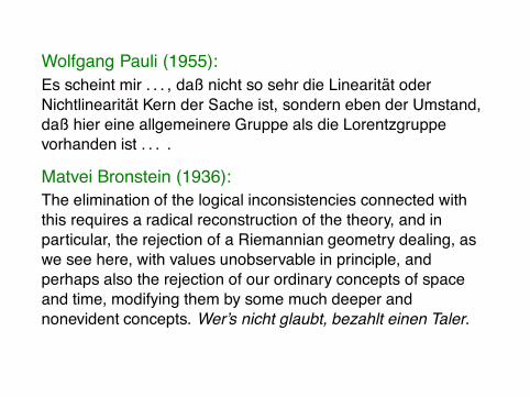
Wolfgang Pauli (1955):Es scheint mir . . . , daß nicht so sehr die Linearitat oderNichtlinearitat Kern der Sache ist, sondern eben der Umstand,daß hier eine allgemeinere Gruppe als die Lorentzgruppevorhanden ist . . . .
Matvei Bronstein (1936):The elimination of the logical inconsistencies connected withthis requires a radical reconstruction of the theory, and inparticular, the rejection of a Riemannian geometry dealing, aswe see here, with values unobservable in principle, andperhaps also the rejection of our ordinary concepts of spaceand time, modifying them by some much deeper andnonevident concepts. Wer’s nicht glaubt, bezahlt einen Taler.
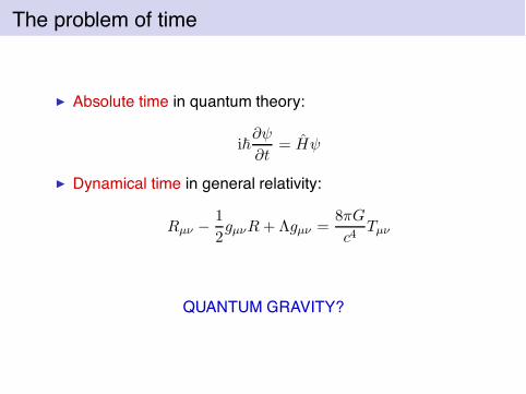
The problem of time
! Absolute time in quantum theory:
i!!"
!t= H"
! Dynamical time in general relativity:
Rµ! !1
2gµ!R + !gµ! =
8#G
c4Tµ!
QUANTUM GRAVITY?
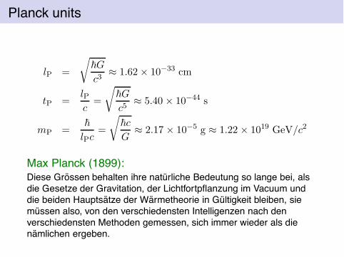
Planck units
lP =
!
!G
c3" 1.62 # 10!33 cm
tP =lPc
=
!
!G
c5" 5.40 # 10!44 s
mP =!
lPc=
!
!c
G" 2.17 # 10!5 g " 1.22 # 1019 GeV/c2
Max Planck (1899):Diese Grossen behalten ihre naturliche Bedeutung so lange bei, alsdie Gesetze der Gravitation, der Lichtfortpflanzung im Vacuum unddie beiden Hauptsatze der Warmetheorie in Gultigkeit bleiben, siemussen also, von den verschiedensten Intelligenzen nach denverschiedensten Methoden gemessen, sich immer wieder als dienamlichen ergeben.
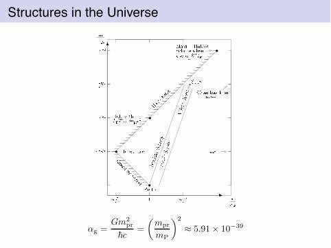
Structures in the Universe
$g =Gm2
pr
!c=
"mpr
mP
#2
" 5.91 # 10!39
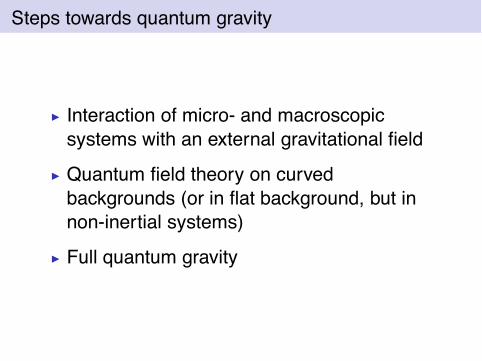
Steps towards quantum gravity
! Interaction of micro- and macroscopicsystems with an external gravitational field
! Quantum field theory on curvedbackgrounds (or in flat background, but innon-inertial systems)
! Full quantum gravity
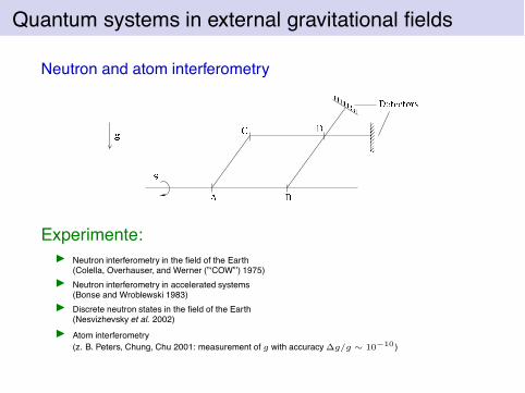
Quantum systems in external gravitational fields
Neutron and atom interferometry
Experimente:! Neutron interferometry in the field of the Earth
(Colella, Overhauser, and Werner (”‘COW”’) 1975)! Neutron interferometry in accelerated systems
(Bonse and Wroblewski 1983)! Discrete neutron states in the field of the Earth
(Nesvizhevsky et al. 2002)! Atom interferometry
(z. B. Peters, Chung, Chu 2001: measurement of g with accuracy !g/g ! 10!10 )
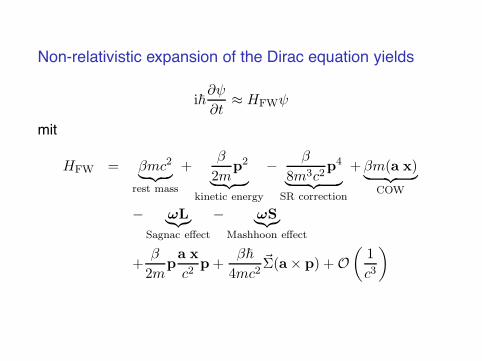
Non-relativistic expansion of the Dirac equation yields
i!!"
!t" HFW"
mit
HFW = %mc2
$ %& '
rest mass
+%
2mp2
$ %& '
kinetic energy
!%
8m3c2p4
$ %& '
SR correction
+%m(a x)$ %& '
COW
! !L$%&'
Sagnac e!ect
! !S$%&'
Mashhoon e!ect
+%
2mpa x
c2p +
%!
4mc2&"(a # p) + O
"1
c3
#
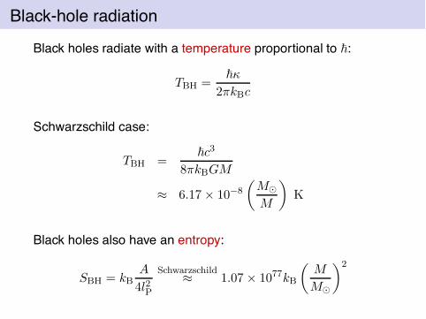
Black-hole radiation
Black holes radiate with a temperature proportional to !:
TBH =!'
2#kBc
Schwarzschild case:
TBH =!c3
8#kBGM
" 6.17 # 10!8
"M"
M
#
K
Black holes also have an entropy:
SBH = kBA
4l2P
Schwarzschild" 1.07 # 1077kB
"M
M"
#2
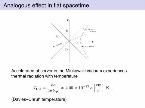
Analogous effect in flat spacetime
IV
III
II Beschl.-Horizont
I X
T
= constant = constantτ ρ
Accelerated observer in the Minkowski vacuum experiencesthermal radiation with temperature
TDU =!a
2#kBc" 4.05 # 10!23 a
(cm
s2
)
K .
(Davies–Unruh temperature)
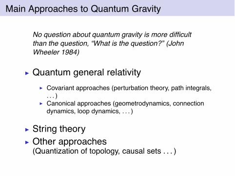
Main Approaches to Quantum Gravity
No question about quantum gravity is more difficultthan the question, “What is the question?” (JohnWheeler 1984)
! Quantum general relativity! Covariant approaches (perturbation theory, path integrals,
. . . )! Canonical approaches (geometrodynamics, connection
dynamics, loop dynamics, . . . )
! String theory! Other approaches
(Quantization of topology, causal sets . . . )
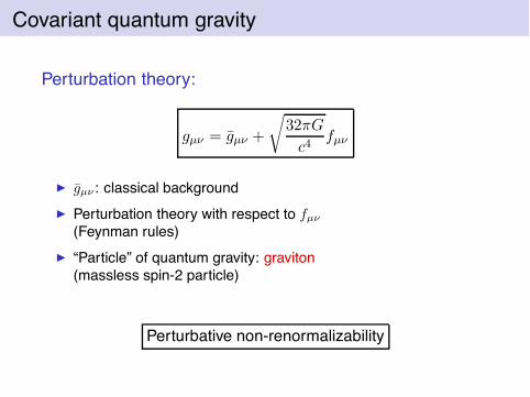
Covariant quantum gravity
Perturbation theory:
gµ! = gµ! +
!
32#G
c4fµ!
! gµ! : classical background! Perturbation theory with respect to fµ!
(Feynman rules)! “Particle” of quantum gravity: graviton
(massless spin-2 particle)
Perturbative non-renormalizability
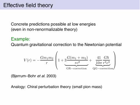
Effective field theory
Concrete predictions possible at low energies(even in non-renormalizable theory)
Example:Quantum gravitational correction to the Newtonian potential
V (r) = !Gm1m2
r
*
++,
1 + 3G(m1 + m2)
rc2$ %& '
GR!correction
+41
10#
G!
r2c3$ %& '
QG!correction
-
.
./
(Bjerrum–Bohr et al. 2003)
Analogy: Chiral perturbation theory (small pion mass)
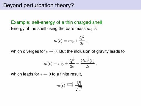
Beyond perturbation theory?
Example: self-energy of a thin charged shellEnergy of the shell using the bare mass m0 is
m(() = m0 +Q2
2(,
which diverges for ( $ 0. But the inclusion of gravity leads to
m(() = m0 +Q2
2(!
Gm2(()
2(,
which leads for ( $ 0 to a finite result,
m(()"#0!$
|Q|%G
.
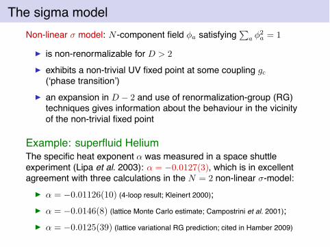
The sigma modelNon-linear ) model: N -component field *a satisfying
0
a *2a = 1
! is non-renormalizable for D > 2
! exhibits a non-trivial UV fixed point at some coupling gc
(‘phase transition’)! an expansion in D ! 2 and use of renormalization-group (RG)
techniques gives information about the behaviour in the vicinityof the non-trivial fixed point
Example: superfluid HeliumThe specific heat exponent $ was measured in a space shuttleexperiment (Lipa et al. 2003): $ = !0.0127(3), which is in excellentagreement with three calculations in the N = 2 non-linear )-model:
! $ = !0.01126(10) (4-loop result; Kleinert 2000);! $ = !0.0146(8) (lattice Monte Carlo estimate; Campostrini et al. 2001);! $ = !0.0125(39) (lattice variational RG prediction; cited in Hamber 2009)
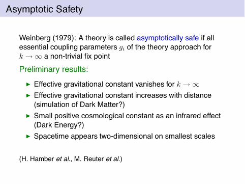
Asymptotic Safety
Weinberg (1979): A theory is called asymptotically safe if allessential coupling parameters gi of the theory approach fork $ & a non-trivial fix point
Preliminary results:! Effective gravitational constant vanishes for k $ &! Effective gravitational constant increases with distance
(simulation of Dark Matter?)! Small positive cosmological constant as an infrared effect
(Dark Energy?)! Spacetime appears two-dimensional on smallest scales
(H. Hamber et al., M. Reuter et al.)
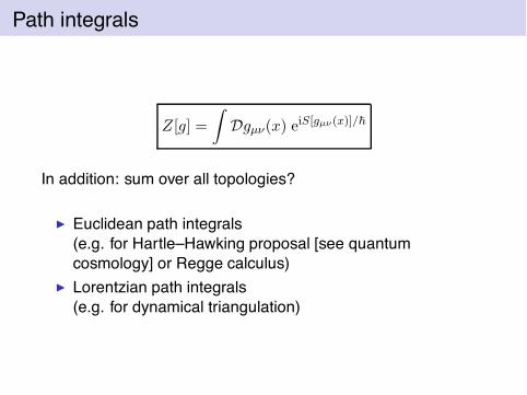
Path integrals
Z[g] =
1
Dgµ!(x) eiS[gµ!(x)]/!
In addition: sum over all topologies?
! Euclidean path integrals(e.g. for Hartle–Hawking proposal [see quantumcosmology] or Regge calculus)
! Lorentzian path integrals(e.g. for dynamical triangulation)
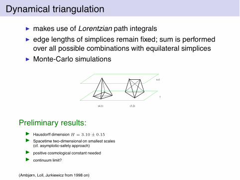
Dynamical triangulation
! makes use of Lorentzian path integrals! edge lengths of simplices remain fixed; sum is performed
over all possible combinations with equilateral simplices! Monte-Carlo simulations
t
t+1
(4,1) (3,2)
Preliminary results:! Hausdorff dimension H = 3.10 ± 0.15
! Spacetime two-dimensional on smallest scales(cf. asymptotic-safety approach)
! positive cosmological constant needed! continuum limit?
(Ambjørn, Loll, Jurkiewicz from 1998 on)
A brief history of early covariant quantum gravity
! L. Rosenfeld, Uber die Gravitationswirkungen des Lichtes,Annalen der Physik (1930)
! M. P. Bronstein, Quantentheorie schwacher Gravitationsfelder,Physikalische Zeitschrift der Sowjetunion (1936)
! S. Gupta, Quantization of Einstein’s Gravitational Field: LinearApproximation, Proceedings of the Royal Society (1952)
! C. Misner, Feynman quantization of general relativity, Reviews ofModern Physics (1957)
! R. P. Feynman, Quantum theory of gravitation, Acta PhysicaPolonica (1963)
! B. S. DeWitt, Quantum theory of gravity II, III, Physical Review(1967)
Canonical quantum gravity
Central equations are constraints:
H# = 0
Different canonical approaches! Geometrodynamics –
metric and extrinsic curvature! Connection dynamics –
connection (Aia) and coloured electric field (Ea
i )! Loop dynamics –
flux of Eai and holonomy
Erwin Schrodinger 1926:We know today, in fact, that our classical mechanics fails forvery small dimensions of the path and for very great curvatures.Perhaps this failure is in strict analogy with the failure ofgeometrical optics . . . that becomes evident as soon as theobstacles or apertures are no longer great compared with thereal, finite, wavelength. . . . Then it becomes a question ofsearching for an undulatory mechanics, and the most obviousway is by an elaboration of the Hamiltonian analogy on the linesof undulatory optics.1
1wir wissen doch heute, daß unsere klassische Mechanik bei sehr kleinenBahndimensionen und sehr starken Bahnkrummungen versagt. Vielleicht istdieses Versagen eine volle Analogie zum Versagen der geometrischen Optik. . . , das bekanntlich eintritt, sobald die ‘Hindernisse’ oder ‘Offnungen’ nichtmehr groß sind gegen die wirkliche, endliche Wellenlange. . . . Dann gilt es,eine ‘undulatorische Mechanik’ zu suchen – und der nachstliegende Wegdazu ist wohl die wellentheoretische Ausgestaltung des HamiltonschenBildes.
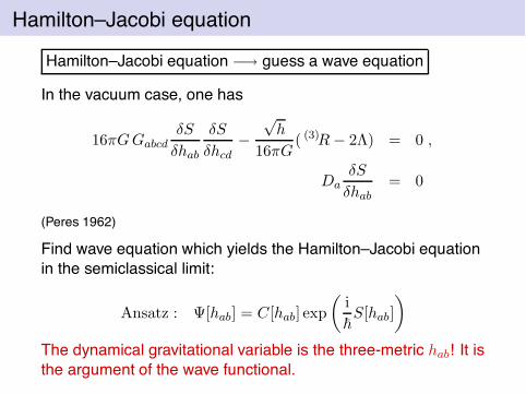
Hamilton–Jacobi equation
Hamilton–Jacobi equation !$ guess a wave equation
In the vacuum case, one has
16#GGabcd+S
+hab
+S
+hcd!
%h
16#G( (3)R ! 2!) = 0 ,
Da+S
+hab= 0
(Peres 1962)
Find wave equation which yields the Hamilton–Jacobi equationin the semiclassical limit:
Ansatz : #[hab] = C[hab] exp
"i
!S[hab]
#
The dynamical gravitational variable is the three-metric hab! It isthe argument of the wave functional.
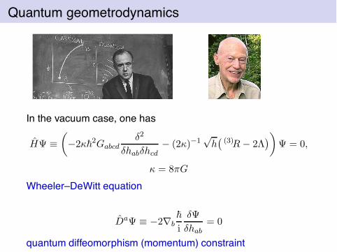
Quantum geometrodynamics
In the vacuum case, one has
H# '"
!2'!2Gabcd
+2
+hab+hcd! (2')!1
%h2
(3)R ! 2!3#
# = 0,
' = 8#G
Wheeler–DeWitt equation
Da# ' !2(b!
i
+#
+hab= 0
quantum diffeomorphism (momentum) constraint
Problem of time
! no external time present; spacetime has disappeared!! local intrinsic time can be defined through local
hyperbolic structure of Wheeler–DeWitt equation(‘wave equation’)
! related problem: Hilbert-space problem –which inner product, if any, to choose between wavefunctionals?
! Schrodinger inner product?! Klein–Gordon inner product?
! Problem of observables
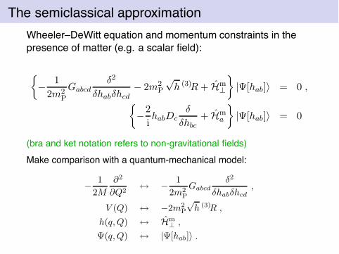
The semiclassical approximationWheeler–DeWitt equation and momentum constraints in thepresence of matter (e.g. a scalar field):
4
!1
2m2P
Gabcd+2
+hab+hcd! 2m2
P
%h (3)R + Hm
$
5
|#[hab]) = 0 ,
4
!2
ihabDc
+
+hbc+ Hm
a
5
|#[hab]) = 0
(bra and ket notation refers to non-gravitational fields)Make comparison with a quantum-mechanical model:
!1
2M
!2
!Q2* !
1
2m2P
Gabcd+2
+hab+hcd,
V (Q) * !2m2P
%h (3)R ,
h(q, Q) * Hm" ,
#(q, Q) * |#[hab]) .
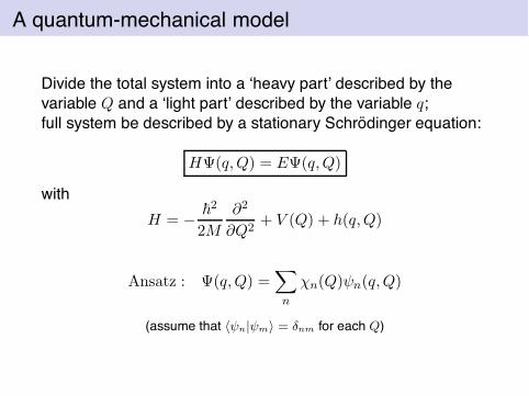
A quantum-mechanical model
Divide the total system into a ‘heavy part’ described by thevariable Q and a ‘light part’ described by the variable q;full system be described by a stationary Schrodinger equation:
H#(q,Q) = E#(q,Q)
withH = !
!2
2M
!2
!Q2+ V (Q) + h(q,Q)
Ansatz : #(q,Q) =6
n
,n(Q)"n(q,Q)
(assume that !!n|!m" = "nm for each Q)
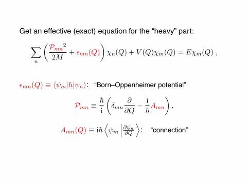
Get an effective (exact) equation for the “heavy” part:
6
n
"Pmn
2
2M+ (mn(Q)
#
,n(Q) + V (Q),m(Q) = E,m(Q) ,
(mn(Q) ' +"m|h|"n): “Born–Oppenheimer potential”
Pmn '!
i
"
+mn!
!Q!
i
!Amn
#
,
Amn(Q) ' i!7
"m
888#$n#Q
9
: “connection”
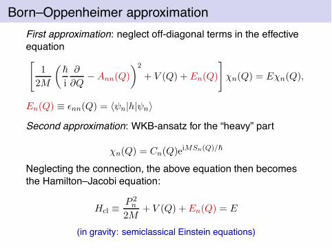
Born–Oppenheimer approximationFirst approximation: neglect off-diagonal terms in the effectiveequation:
1
2M
"!
i
!
!Q! Ann(Q)
#2
+ V (Q) + En(Q)
;
,n(Q) = E,n(Q),
En(Q) ' (nn(Q) = +"n|h|"n)
Second approximation: WKB-ansatz for the “heavy” part
,n(Q) = Cn(Q)eiMSn(Q)/!
Neglecting the connection, the above equation then becomesthe Hamilton–Jacobi equation:
Hcl 'P 2
n
2M+ V (Q) + En(Q) = E
(in gravity: semiclassical Einstein equations)
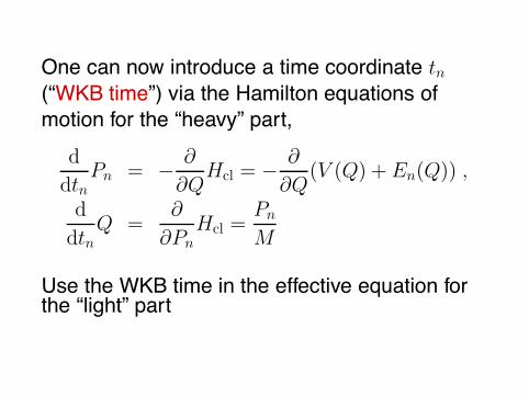
One can now introduce a time coordinate tn(“WKB time”) via the Hamilton equations ofmotion for the “heavy” part,
d
dtnPn = !
!
!QHcl = !
!
!Q(V (Q) + En(Q)) ,
d
dtnQ =
!
!PnHcl =
Pn
M
Use the WKB time in the effective equation forthe “light” part
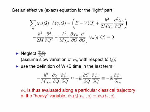
Get an effective (exact) equation for the “light” part:
6
n
,n(Q)
<
h(q,Q) !"
E ! V (Q) +!2
2M,n
!2,n
!Q2
#
!!2
2M
!2
!Q2!
!2
M,n
!,n
!Q
!
!Q
=
"n(q,Q) = 0
! Neglect #2%n
#Q2
(assume slow variation of "n with respect to Q);! use the definition of WKB time in the last term:
!!2
M,n
!,n
!Q
!"n
!Q" !i!
!Sn
!Q
!"n
!Q' !i!
!"n
!tn
"n is thus evaluated along a particular classical trajectoryof the “heavy” variable, "n(Q(tn), q) ' "n(tn, q).
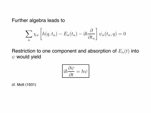
Further algebra leads to6
n
"n
<
h(q, tn) ! En(tn) ! i!!
!tn
=
#n(tn, q) = 0
Restriction to one component and absorption of En(t) into# would yield
i!!#
!t= h#
cf. Mott (1931)
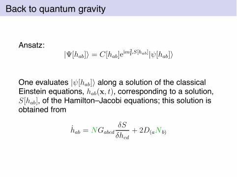
Back to quantum gravity
Ansatz:|![hab]) = C[hab]e
im2P
S[hab]|#[hab])
One evaluates |#[hab]) along a solution of the classicalEinstein equations, hab(x, t), corresponding to a solution,S[hab], of the Hamilton–Jacobi equations; this solution isobtained from
hab = NGabcd$S
$hcd+ 2D(aN b)
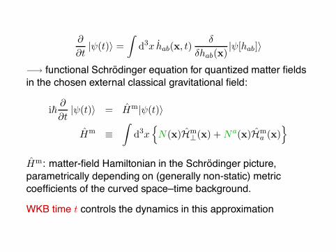
!
!t|"(t)) =
1
d3x hab(x, t)+
+hab(x)|"[hab])
!$ functional Schrodinger equation for quantized matter fieldsin the chosen external classical gravitational field:
i!!
!t|"(t)) = Hm|"(t))
Hm '1
d3x>
N(x)Hm$(x) + Na(x)Hm
a (x)?
Hm: matter-field Hamiltonian in the Schrodinger picture,parametrically depending on (generally non-static) metriccoefficients of the curved space–time background.
WKB time t controls the dynamics in this approximation
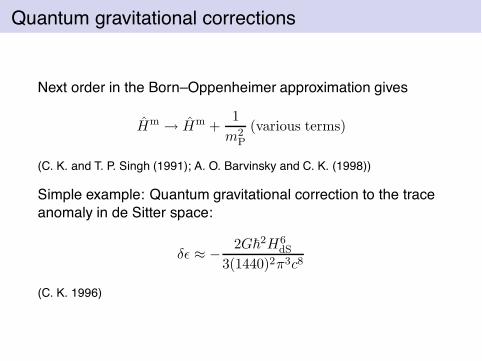
Quantum gravitational corrections
Next order in the Born–Oppenheimer approximation gives
Hm $ Hm +1
m2P
(various terms)
(C. K. and T. P. Singh (1991); A. O. Barvinsky and C. K. (1998))
Simple example: Quantum gravitational correction to the traceanomaly in de Sitter space:
+( " !2G!2H6
dS
3(1440)2#3c8
(C. K. 1996)
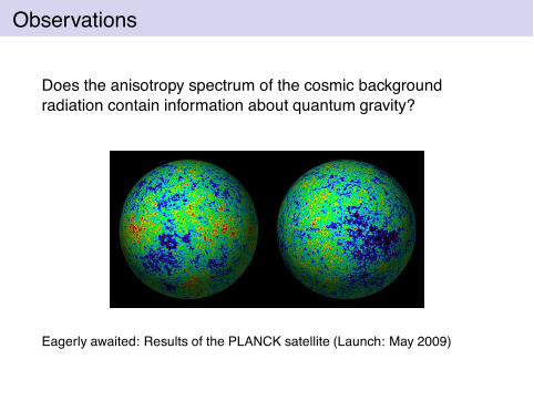
Observations
Does the anisotropy spectrum of the cosmic backgroundradiation contain information about quantum gravity?
Eagerly awaited: Results of the PLANCK satellite (Launch: May 2009)
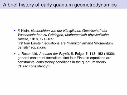
A brief history of early quantum geometrodynamics
! F. Klein, Nachrichten von der Koniglichen Gesellschaft derWissenschaften zu Gottingen, Mathematisch-physikalischeKlasse, 1918, 171–189:first four Einstein equations are “Hamiltonian”and “momentumdensity” equations
! L. Rosenfeld, Annalen der Physik, 5. Folge, 5, 113–152 (1930):general constraint formalism; first four Einstein equations areconstraints; consistency conditions in the quantum theory(“Dirac consistency”)
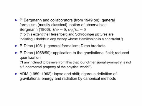
! P. Bergmann and collaborators (from 1949 on): generalformalism (mostly classical); notion of observablesBergmann (1966): H" = 0, !"/!t = 0(“To this extent the Heisenberg and Schrodinger pictures areindistinguishable in any theory whose Hamiltonian is a constraint.”)
! P. Dirac (1951): general formalism; Dirac brackets! P. Dirac (1958/59): application to the gravitational field; reduced
quantization(“I am inclined to believe from this that four-dimensional symmetry is nota fundamental property of the physical world.”)
! ADM (1959–1962): lapse and shift; rigorous definition ofgravitational energy and radiation by canonical methods
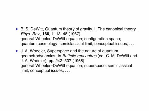
! B. S. DeWitt, Quantum theory of gravity. I. The canonical theory.Phys. Rev., 160, 1113–48 (1967):general Wheeler–DeWitt equation; configuration space;quantum cosmology; semiclassical limit; conceptual issues, . . .
! J. A. Wheeler, Superspace and the nature of quantumgeometrodynamics. In Battelle rencontres (ed. C. M. DeWitt andJ. A. Wheeler), pp. 242–307 (1968):general Wheeler–DeWitt equation; superspace; semiclassicallimit; conceptual issues; . . .
Path Integral satisfies Constraints
! Quantum mechanics: path integral satisfiesSchrodinger equation
! Quantum gravity: path integral satisfiesWheeler–DeWitt equation anddiffeomorphism constraints
A. O. Barvinsky (1998): direct check in the one-loopapproximation that the quantum-gravitational path integralsatisfies the constraints!$ connection between covariant and canonical approachapplication in quantum cosmology: no-boundary condition
Ashtekar’s new variables
! new momentum variable: densitized version of triad,Ea
i (x) :=@
h(x)eai (x) ;
! new configuration variable: ‘connection’ ,GAi
a(x) := $ia(x) + %Ki
a(x)
{Aia(x), Eb
j (y)} = 8#%+ij+
ba+(x, y)
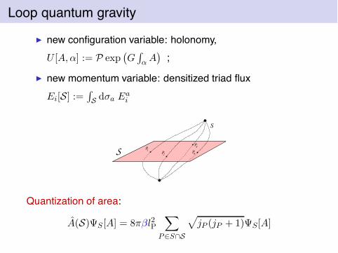
Loop quantum gravity
! new configuration variable: holonomy,U [A,$] := P exp
2
GA
& A3
;
! new momentum variable: densitized triad fluxEi[S] :=
A
Sd)a Ea
i
S
S
P1P2
P34P
Quantization of area:
A(S)#S [A] = 8#%l2P6
P%S&S
@
jP (jP + 1)#S[A]
String theory
Important properties:
! Inclusion of gravity unavoidable! Gauge invariance, supersymmetry, higher dimensions! Unification of all interactions! Perturbation theory probably finite at all orders, but sum
diverges! Only three fundamental constants: !, c, ls! Branes as central objects! Dualities connect different string theories
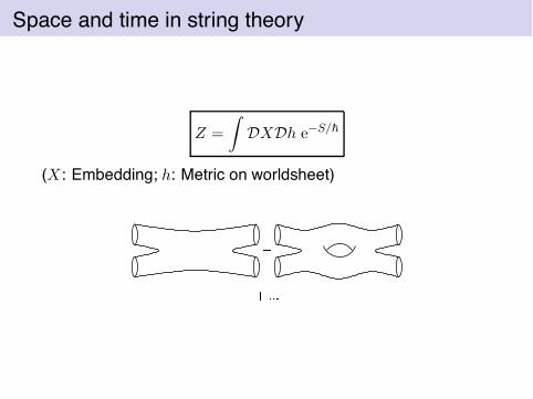
Space and time in string theory
Z =
1
DXDh e!S/!
(X: Embedding; h: Metric on worldsheet)
Absence of quantum anomalies !$
! Background fields obey Einstein equations up to O(l2s );can be derived from an effective action
! Constraint on the number of spacetime dimensions:10 resp. 11
Generalized uncertainty relation:
%x ,!
%p+
l2s!%p
Problems
! Too many “string vacua” (problem of landscape)! No background independence?! Standard model of particle physics?! What is the role of the 11th dimension? What is
M-theory?! Experiments?
Black holes
Microscopic explanation of entropy?
SBH = kBA
4l2P
! Loop quantum gravity: microscopic degrees of freedomare the spin networks; SBH only follows for a specificchoice of %: % = 0.237532 . . .
! String theory: microscopic degrees of freedom are the“D-branes”; SBH only follows for special (extremal ornear-extremal) black holes
! Quantum geometrodynamics: e.g. S - A in the LTB model
Problem of information loss! Final phase of evaporation?! Fate of information is a consequence of the fundamental
theory (unitary or non-unitary)! Problem does not arise in the semiclassical approximation
(thermal character of Hawking radiation follows fromdecoherence)
! Empirical problems:! Are there primordial black holes?! Can black holes be generated in accelerators?
Primordial black holes
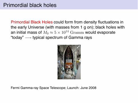
Primordial Black Holes could form from density fluctuations inthe early Universe (with masses from 1 g on); black holes withan initial mass of M0 " 5 # 1014 Gramm would evaporate“today” !$ typical spectrum of Gamma rays
Fermi Gamma-ray Space Telescope; Launch: June 2008
Generation of mini black holes at the LHC?
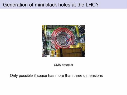
CMS detector
Only possible if space has more than three dimensions
My own research on quantum black holes
! Primordial black holes from density fluctuations ininflationary models
! Quasi-normal modes and the Hawking temperature! Decoherence of quantum black holes and its relevance for
the problem of information loss! Hawking temperature from solutions to the
Wheeler–DeWitt equation (for the LTB model) as well asquantum gravitational corrections
! Area law for the entropy from solutions to theWheeler–DeWitt equation (for the 2+1-dimensional LTBmodel)
! Origin of corrections to the area law! Model for black-hole evaporation
Why Quantum Cosmology?
Gell-Mann and Hartle 1990:Quantum mechanics is best and most fundamentallyunderstood in the framework of quantum cosmology.
! Quantum theory is universally valid:Application to the Universe as a whole as the only closedquantum system in the strict sense
! Need quantum theory of gravity, since gravity dominateson large scales
Quantization of a Friedmann Universe
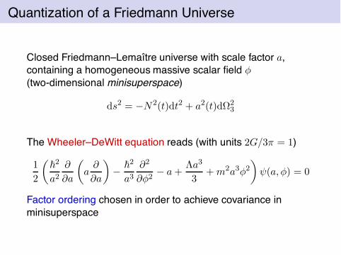
Closed Friedmann–Lemaıtre universe with scale factor a,containing a homogeneous massive scalar field *(two-dimensional minisuperspace)
ds2 = !N2(t)dt2 + a2(t)d&23
The Wheeler–DeWitt equation reads (with units 2G/3# = 1)
1
2
"!2
a2
!
!a
"
a!
!a
#
!!2
a3
!2
!*2! a +
!a3
3+ m2a3*2
#
"(a,*) = 0
Factor ordering chosen in order to achieve covariance inminisuperspace
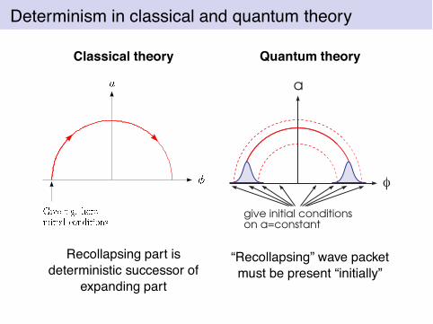
Determinism in classical and quantum theory
Classical theory
Recollapsing part isdeterministic successor of
expanding part
Quantum theory
φ
a
give initial conditions on a=constant
“Recollapsing” wave packetmust be present “initially”
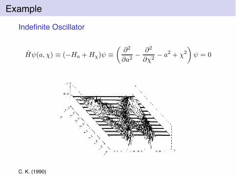
Example
Indefinite Oscillator
H"(a,,) ' (!Ha + H%)" '"
!2
!a2!
!2
!,2! a2 + ,2
#
" = 0
C. K. (1990)
Validity of Semiclassical Approximation?
Closed universe: ‘Final condition’ #a$&!$ 0
.
wave packets in general disperse
.
WKB approximation not always validSolution: Decoherence (see below)
Introduction of inhomogeneities
Describe small inhomogeneities by multipoles {xn} around theminisuperspace variables (e.g. a and *)
B
H0 +6
n
Hn(a,*, xn)
C
#($,*, {xn}) = 0
(Halliwell and Hawking 1985)
If "0 is of WKB form, "0 " C exp(iS0/!) (with a slowly varyingprefactor C), one will get with # = "o
D
n "n,
i!!"n
!t" Hn"n
with!
!t' (S0 ·(
t: ‘WKB time’ – controls the dynamics in this approximation
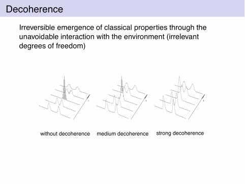
Decoherence
Irreversible emergence of classical properties through theunavoidable interaction with the environment (irrelevantdegrees of freedom)
without decoherence
t
(a)
medium decoherence
t
(b)
strong decoherence
t
(c)
Decoherence in quantum cosmology
Quantum gravity / superposition of different metricsDecoherence?
! ‘System’: Global degrees of freedom (radius of Universe,inflaton field, . . . )
! ‘Environment’: Density fluctuations, gravitational waves,other fields
(Zeh 1986, C.K. 1987)
Example: Scale factor a of de Sitter space (a - eHIt) (‘system’)is decohered by gravitons (‘environment’) according to
-0(a, a') $ -0(a, a') exp2
!CH3I a(a ! a')2
3
, C > 0
The Universe assumes classical properties at the ‘beginning’ ofthe inflationary phase(Barvinsky, Kamenshchik, C.K. 1999)

Time from Symmetry Breaking
Analogy from molecular physics: emergence of chirality
1
23
41
2 3
4V(z)
|1>
|2>
dynamical origin: decoherence due to scattering with light or airmolecules
quantum cosmology: decoherence between exp(iS0/!)- andexp(!iS0/!)-part of wave function through interaction withmultipolesone example for decoherence factor:exp
“
#"mH2
0a3
128!
”
$ exp`
#1043´
(C. K. 1992)
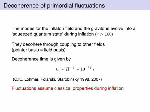
Decoherence of primordial fluctuations
The modes for the inflaton field and the gravitons evolve into a‘squeezed quantum state’ during inflation (r > 100)
They decohere through coupling to other fields(pointer basis = field basis)
Decoherence time is given by
td 0 H!1I 0 10!34 s
(C.K., Lohmar, Polarski, Starobinsky 1998, 2007)
Fluctuations assume classical properties during inflation
Interpretation of quantum cosmology
Both quantum general relativity and string theory preserve thelinear structure for the quantum states=/ strict validity of the superposition principleonly interpretation so far: Everett interpretation(with decoherence as an essential part)
B. S. DeWitt 1967:Everett’s view of the world is a very natural one to adopt in thequantum theory of gravity, where one is accustomed to speakwithout embarassment of the ‘wave function of the universe.’ Itis possible that Everett’s view is not only natural but essential.
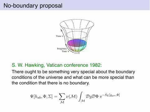
No-boundary proposal
t
Time
Time
τ = 0τ
Imaginary
S. W. Hawking, Vatican conference 1982:There ought to be something very special about the boundaryconditions of the universe and what can be more special thanthe condition that there is no boundary.
#[hab,',"] =6
M
.(M)
1
M
DgD' e!SE[gµ! ,"]
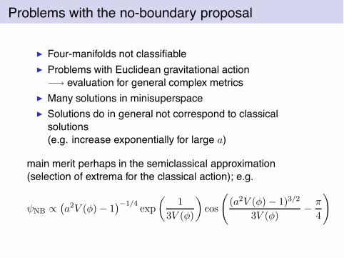
Problems with the no-boundary proposal
! Four-manifolds not classifiable! Problems with Euclidean gravitational action
!$ evaluation for general complex metrics! Many solutions in minisuperspace! Solutions do in general not correspond to classical
solutions(e.g. increase exponentially for large a)
main merit perhaps in the semiclassical approximation(selection of extrema for the classical action); e.g.
"NB -2
a2V (*) ! 13!1/4
exp
"1
3V (*)
#
cos
B
(a2V (*) ! 1)3/2
3V (*)!
#
4
C
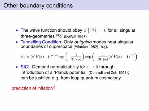
Other boundary conditions
! The wave function should obey #E(3)G
F
= 0 for all singularthree-geometries (3)G (DeWitt 1967)
! Tunnelling Condition: Only outgoing modes near singularboundaries of superspace (Vilenkin 1982); e.g.
!T % (a2V (#)#1)"1/4 exp
„
#1
3V (#)
«
exp
„
#i
3V (#)(a2V (#) # 1)3/2
«
! SIC!: Demand normalizability for a $ 0 throughintroduction of a ‘Planck potential’ (Conradi and Zeh 1991);can be justified e.g. from loop quantum cosmology
prediction of inflation?
Criteria for quantum avoidance of singularities
No general agreement!
Sufficient criteria in quantum geometrodynamics:! Vanishing of the wave function at the point of the classical
singularity (dating back to DeWitt 1967)! Spreading of wave packets when approaching the region
of the classical singularity
concerning the second criterium:only in the semiclassical regime (narrow wave packets followingthe classical trajectories) do we have an approximate notion ofgeodesics !$ only in this regime can we apply the classicalsingularity theorems
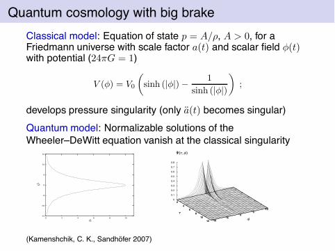
Quantum cosmology with big brakeClassical model: Equation of state p = A/-, A > 0, for aFriedmann universe with scale factor a(t) and scalar field *(t)with potential (24#G = 1)
V (*) = V0
"
sinh (|*|) !1
sinh (|*|)
#
;
develops pressure singularity (only a(t) becomes singular)Quantum model: Normalizable solutions of theWheeler–DeWitt equation vanish at the classical singularity
-15
-10
-5
0
5
10
15
0 2 4 6 8 10a
!
2 4
6 8
10 12 -10
-5 0
5 10
0
0.1
0.2
0.3
0.4
0.5
0.6
0.7
0.8
2 4
6 8
10 12 -10
-5 0
5 10
//
**
!(/,*)!(/,*)
(Kamenshchik, C. K., Sandhofer 2007)
Supersymmetric quantum cosmological billiards
D = 11 supergravity: near spacelike singularitycosmological billiard description based on theKac–Moody group E10 !$ discussion ofWheeler–DeWitt equation
! ! $ 0 near the singularity! ! is generically complex and oscillating
(Kleinschmidt, Koehn, Nicolai 2009)
Quantum phantom cosmology
Classical model: Friedmann universe with scale factor a(t)containing a scalar field with negative kinetic term (‘phantom’)!$ develops a big-rip singularity(- and p diverge as a goes to infinity at a finite time)Quantum model: Wave-packet solutions of the Wheeler–DeWittequation disperse in the region of the classical big-ripsingularity!$ time and the classical evolution come to an end;only a stationary quantum state is leftExhibition of quantum effects at large scales!
(Dabrowski, C. K., Sandhofer 2006)
Loop Quantum Cosmology
! Difference equation instead of Wheeler–DeWitt equation;the latter emerges as an effective description away fromthe Planck scale
! Singularity avoidance (from difference equation or fromeffective Friedmann equation via a bounce)
! Prediction of inflation (?)! Observable effect in the CMB spectrum (?)! but: not yet derived from full loop quantum gravity
(cf. M. Bojowald, C.K., P. Vargas Moniz, arXiv:1005.2471v1 [gr-qc])
Effective equations in loop quantum cosmologyEffective Hamiltonian constraint reads
He! = !3
8#G%2
sin2(0p)
02a3 + Hm ,
where 0 = 2(%
3#%)1/2lP
This leads to a modified Hubble rate:
H2 =8#G
3-
"
1 !-
-c
#
,
where -c = 3/(8#G%202) " 0.41-P
!$ bounces which may prevent singularities(P. Singh, arXiv:0901.2750: “All strong singularities are generically resolvedin loop quantum cosmology.”)
Corresponds to the second of the criteria above (breakdown ofsemiclassical approximation near the classical singularity)
How special is the Universe
Penrose (1981):Entropy of the observed part of the Universe is maximal if all itsmass is in one black hole; the probability for our Universe wouldthen be (updated version from C.K. arXiv:0910.5836)
expG
SkB
H
expG
Smax
kB
H 0exp
2
3.1 # 101043
exp (1.8 # 10121)" exp
2
!1.8 # 101213
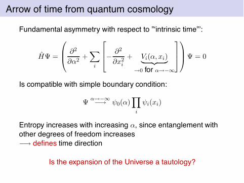
Arrow of time from quantum cosmology
Fundamental asymmetry with respect to ”‘intrinsic time”’:
H# =
*
+,
!2
!$2+6
i
I
JK!
!2
!x2i
+ Vi($, xi)$ %& '
#0 for &#!(
L
MN
-
./# = 0
Is compatible with simple boundary condition:
#&#!(!$ "0($)
O
i
"i(xi)
Entropy increases with increasing $, since entanglement withother degrees of freedom increases!$ defines time direction
Is the expansion of the Universe a tautology?
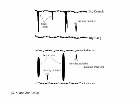
Big Bang
Big Crunch
blackholes
Hawking radiation
black holes
Radius zero
Radius zero
Hawking radiation
Hawking radiationmaximal extension
(C. K. and Zeh 1995)
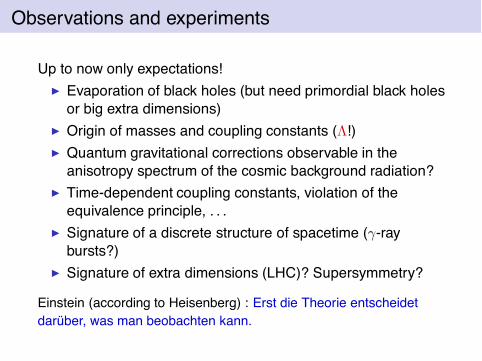
Observations and experiments
Up to now only expectations!! Evaporation of black holes (but need primordial black holes
or big extra dimensions)! Origin of masses and coupling constants (!!)! Quantum gravitational corrections observable in the
anisotropy spectrum of the cosmic background radiation?! Time-dependent coupling constants, violation of the
equivalence principle, . . .! Signature of a discrete structure of spacetime (1-ray
bursts?)! Signature of extra dimensions (LHC)? Supersymmetry?
Einstein (according to Heisenberg) : Erst die Theorie entscheidetdaruber, was man beobachten kann.
More details inC. K., Quantum Gravity, second edition(Oxford 2007).
Recommended