About this presentation
Target audience: Prepared for Dr. Mitsuru Saito’s BYU graduate level class. Feb. 2003.
Please contact Mike Brown at 801-363-4250 or [email protected] if you have comments or questions.
Thanks for your interest in this subject.

WFRC – MAG Travel Demand Model, Version 2.10
Mike Brown,
Muhammad Farhan
Wasatch Front Regional Council
(This isn’t related, I just like it!)
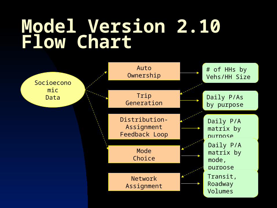
Model Version 2.10 Flow Chart
TripGeneration
Distribution-AssignmentFeedback Loop
ModeChoice
NetworkAssignment
AutoOwnership
# of HHs by Vehs/HH Size
Daily P/As by purpose
Daily P/A matrix by purpose
Daily P/A matrix by mode, purpose
SocioeconomicData
Transit, Roadway Volumes
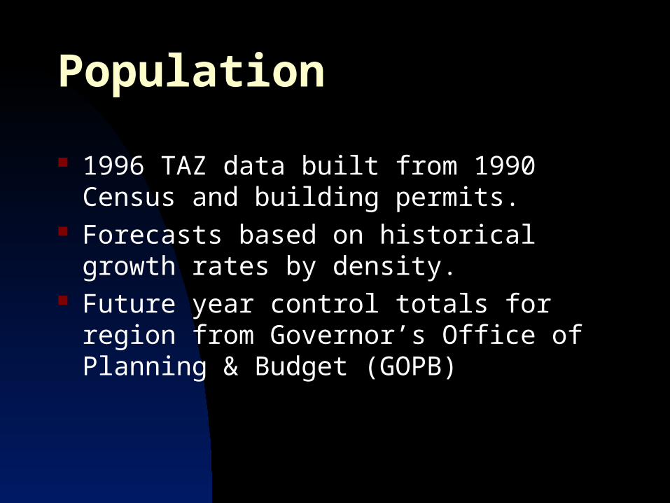
Population
1996 TAZ data built from 1990 Census and building permits.
Forecasts based on historical growth rates by density.
Future year control totals for region from Governor’s Office of Planning & Budget (GOPB)
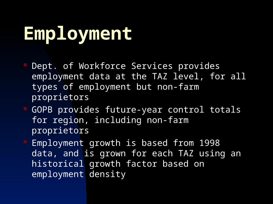
Employment
Dept. of Workforce Services provides employment data at the TAZ level, for all types of employment but non-farm proprietors
GOPB provides future-year control totals for region, including non-farm proprietors
Employment growth is based from 1998 data, and is grown for each TAZ using an historical growth factor based on employment density
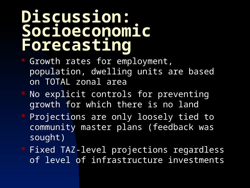
Discussion: Socioeconomic Forecasting Growth rates for employment, population,
dwelling units are based on TOTAL zonal area
No explicit controls for preventing growth for which there is no land
Projections are only loosely tied to community master plans (feedback was sought)
Fixed TAZ-level projections regardless of level of infrastructure investments
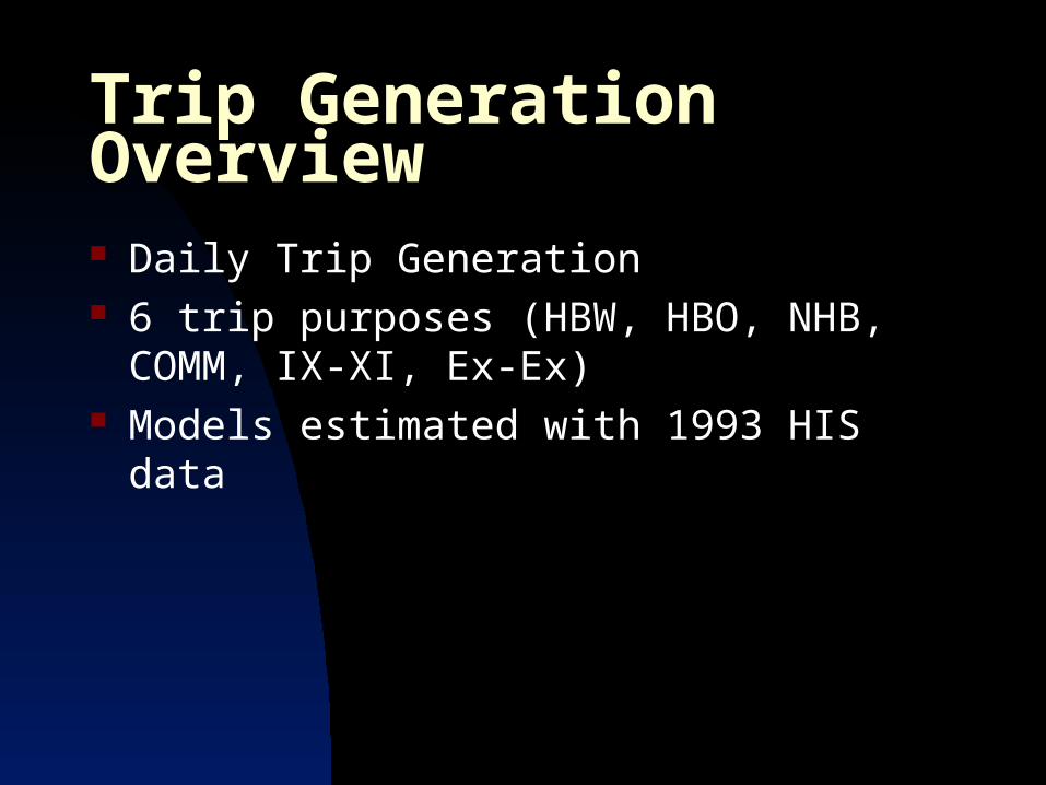
Trip Generation Overview
Daily Trip Generation 6 trip purposes (HBW, HBO, NHB, COMM,
IX-XI, Ex-Ex) Models estimated with 1993 HIS data
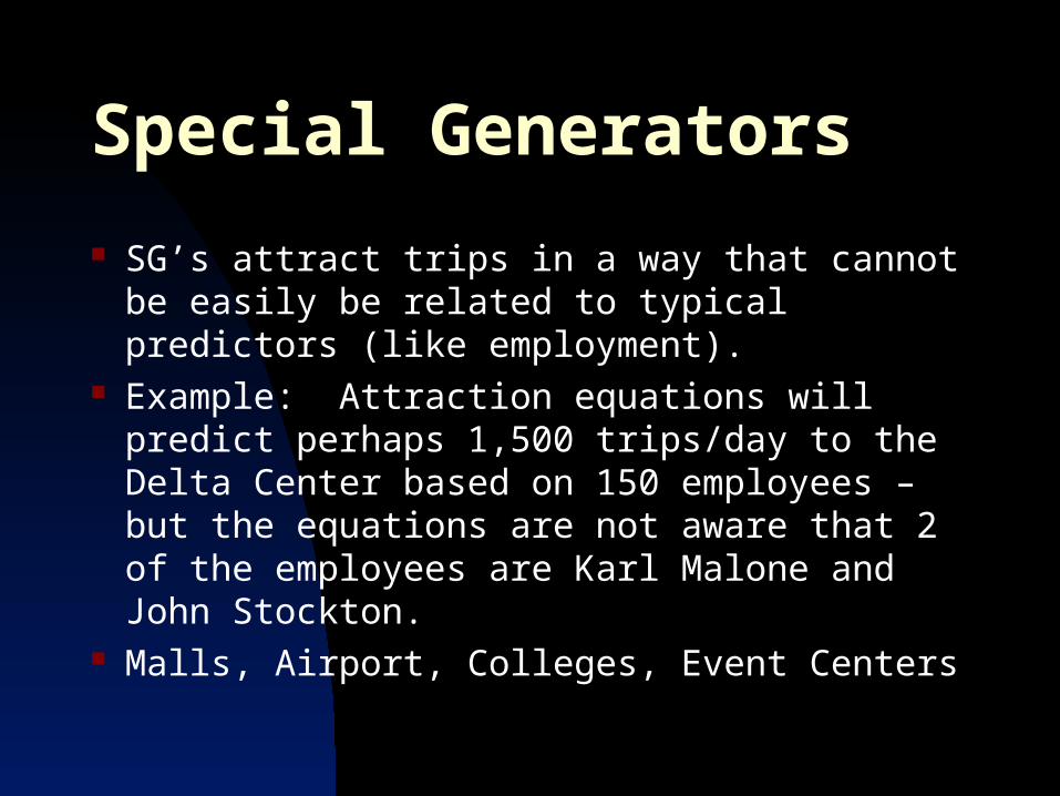
Special Generators
SG’s attract trips in a way that cannot be easily be related to typical predictors (like employment).
Example: Attraction equations will predict perhaps 1,500 trips/day to the Delta Center based on 150 employees – but the equations are not aware that 2 of the employees are Karl Malone and John Stockton.
Malls, Airport, Colleges, Event Centers
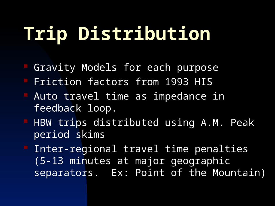
Trip Distribution
Gravity Models for each purpose Friction factors from 1993 HIS Auto travel time as impedance in feedback loop. HBW trips distributed using A.M. Peak period skims Inter-regional travel time penalties (5-13 minutes at
major geographic separators. Ex: Point of the Mountain)
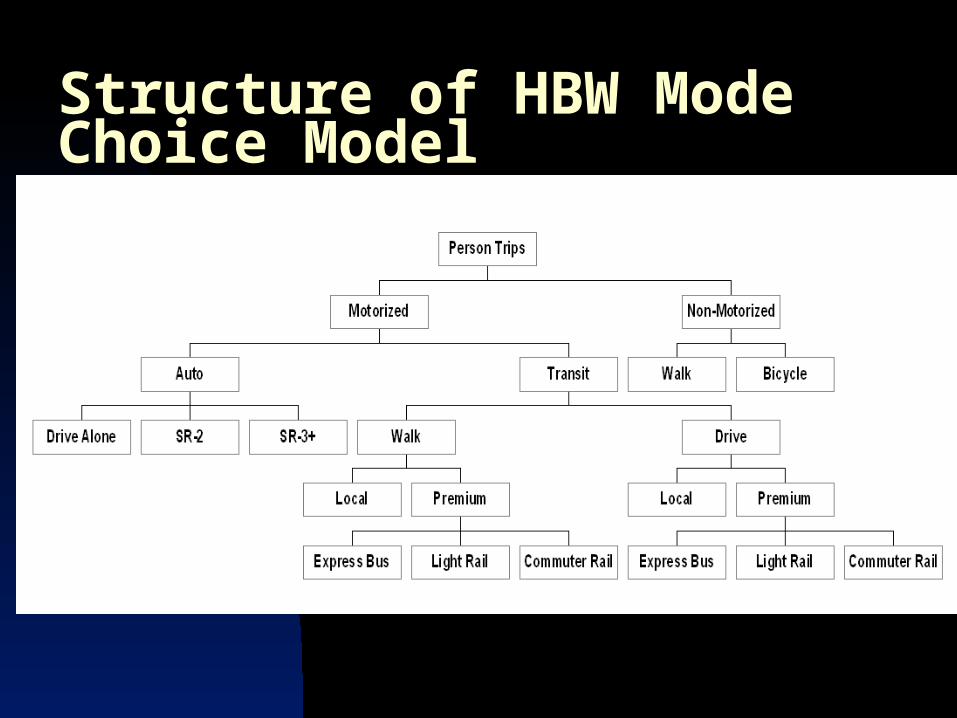
Structure of HBW Mode Choice Model

VMT Comparison (1996)
2003 estimate: 41,000,000 VMT/day; 5,900 lane miles 2030 estimate: 71,000,000 VMT/day; 7,500 lane miles
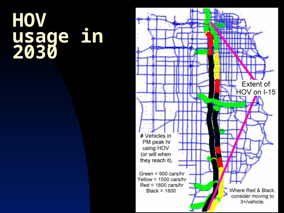
HOV usage in 2030
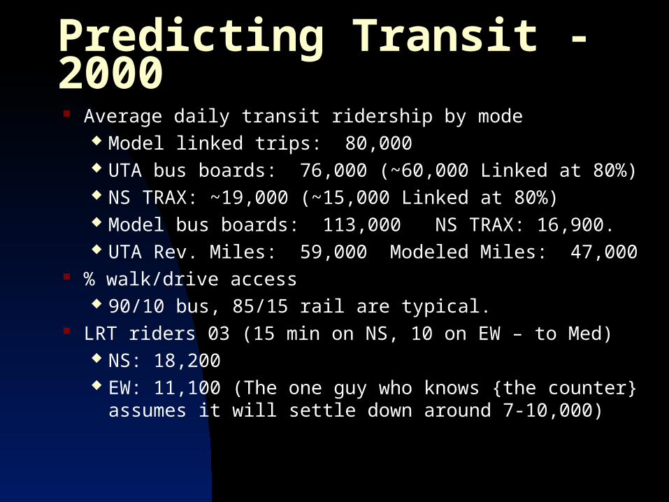
Predicting Transit - 2000 Average daily transit ridership by mode
Model linked trips: 80,000 UTA bus boards: 76,000 (~60,000 Linked at 80%) NS TRAX: ~19,000 (~15,000 Linked at 80%) Model bus boards: 113,000 NS TRAX: 16,900. UTA Rev. Miles: 59,000 Modeled Miles: 47,000
% walk/drive access 90/10 bus, 85/15 rail are typical.
LRT riders 03 (15 min on NS, 10 on EW – to Med) NS: 18,200 EW: 11,100 (The one guy who knows {the counter}
assumes it will settle down around 7-10,000)
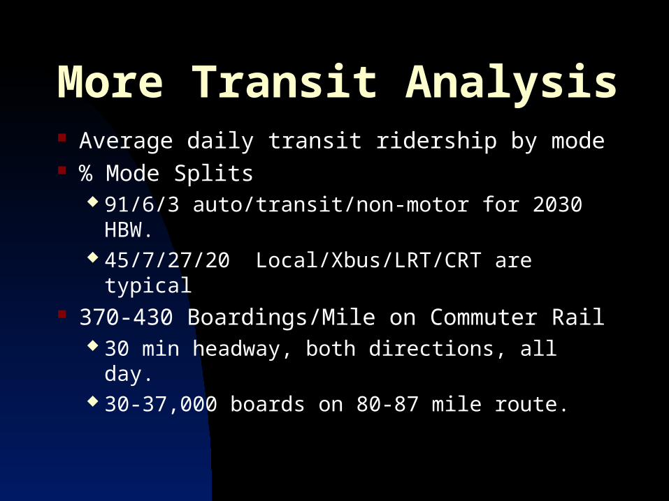
More Transit Analysis Average daily transit ridership by mode % Mode Splits
91/6/3 auto/transit/non-motor for 2030 HBW. 45/7/27/20 Local/Xbus/LRT/CRT are typical
370-430 Boardings/Mile on Commuter Rail 30 min headway, both directions, all day. 30-37,000 boards on 80-87 mile route.

What you should know about models Uses are varied and valuable
Air quality conformity determinations. “Purpose & Need” foundation for EIS work. FTA new starts applications. Long range facility and right-of-way needs.
Historically reliable for major highway predictions. So far, so good on transit.
Traditionally underappreciated for the role they play in defensible processes and decision making
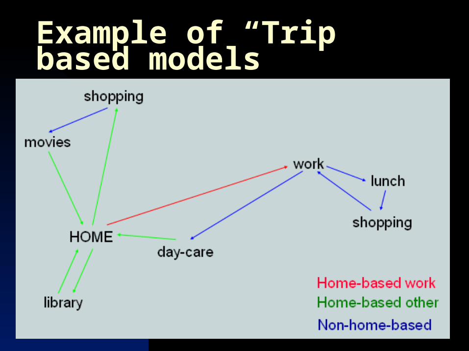
Example of “Trip” based models
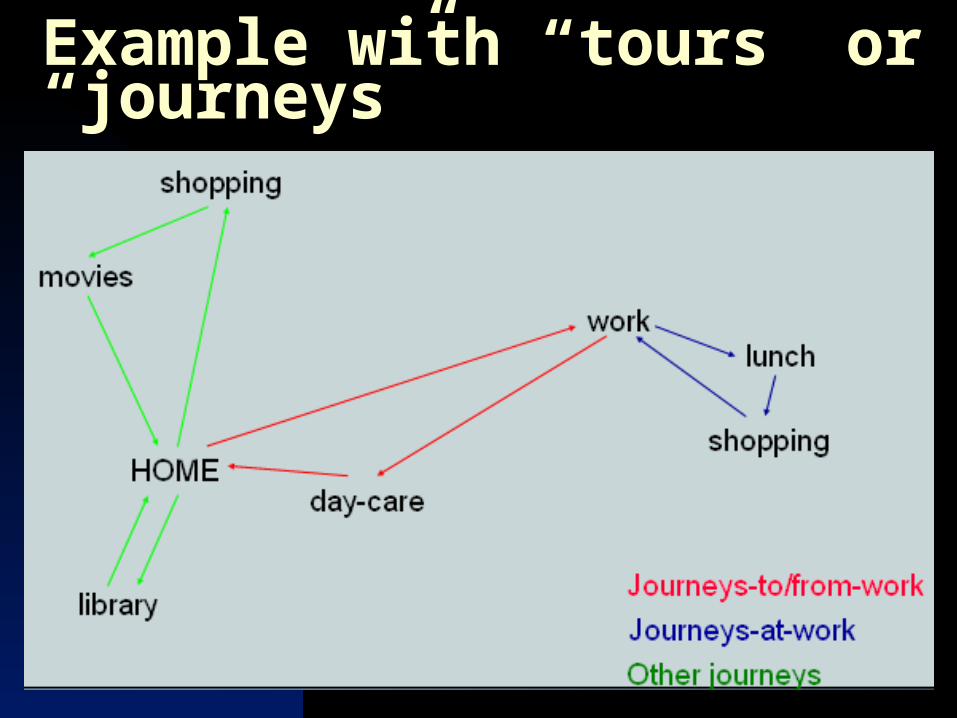
Example with “tours” or “journeys”
Why not do tour based modeling? Still an emerging method that is being
implemented only in San Francisco, Houston, and a few other major cities.
Requires a unique approach to “home interview surveys” – a $500k+ endeavor!
Requires complete rewrite of model with few salvageable elements from previous model – also a $500k+ endeavor!
Recommended