Ab initio nonadiabatic molecular dynamicsTDDFT for ultrafast electronic dynamics
Ivano Tavernelli and Basile Curchod
LCBC EPFL, Lausanne
TDDFT SCHOOLBENASQUE 2014
Ab initio nonadiabatic molecular dynamics
Outline
1 Ab initio molecular dynamicsWhy Quantum Dynamics?
2 Mixed quantum-classical dynamicsEhrenfest dynamicsAdiabatic Born-Oppenheimer dynamicsNonadiabatic Bohmian dynamicsTrajectory Surface Hopping
3 TDDFT-based trajectory surface hoppingNonadiabatic couplings in TDDFT
4 TDDFT-TSH: ApplicationsPhotodissociation of OxiraneOxirane - Crossing between S1 and S0
5 TSH with external time-dependent fields
Ab initio nonadiabatic molecular dynamics
Outline
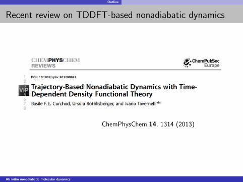
Recent review on TDDFT-based nonadiabatic dynamics
ChemPhysChem,14, 1314 (2013)
Ab initio nonadiabatic molecular dynamics
Ab initio molecular dynamics
1 Ab initio molecular dynamicsWhy Quantum Dynamics?
2 Mixed quantum-classical dynamicsEhrenfest dynamicsAdiabatic Born-Oppenheimer dynamicsNonadiabatic Bohmian dynamicsTrajectory Surface Hopping
3 TDDFT-based trajectory surface hoppingNonadiabatic couplings in TDDFT
4 TDDFT-TSH: ApplicationsPhotodissociation of OxiraneOxirane - Crossing between S1 and S0
5 TSH with external time-dependent fields
Ab initio nonadiabatic molecular dynamics

Ab initio molecular dynamics
Reminder from last lecture: potential energy surfaces
We have electronic structure methods for electronic ground and excited states...Now, we need to propagate the nuclei...
Ab initio nonadiabatic molecular dynamics

Ab initio molecular dynamics
Reminder from last lecture: potential energy surfaces
We have electronic structure methods for electronic ground and excited states...Now, we need to propagate the nuclei...
Ab initio nonadiabatic molecular dynamics
Ab initio molecular dynamics Why Quantum Dynamics?
Why Quantum dynamics?E
nerg
y
Ene
rgy
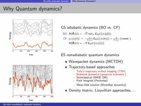
GS adiabatic dynamics (BO vs. CP)
BO MI RI (t) = −∇minρ EKS (φi [ρ])
CP µi |φi (t)〉 = − δδ〈φi |
EKS (φi (r)) + δδ〈φi |
constr.MI RI (t) = −∇EKS (φi (t))
ES nonadiabatic quantum dynamics
Wavepacket dynamics (MCTDH)
Trajectory-based approaches- Tully’s trajectory surface hopping (TSH)- Bohmian dynamics (quantum hydrodyn.)- Semiclassical (WKB, DR)- Path integrals (Pechukas)
- Mean-field solution (Ehrenfest dynamics)
Density matrix, Liouvillian approaches, ...
Ab initio nonadiabatic molecular dynamics
Ab initio molecular dynamics Why Quantum Dynamics?
Why Quantum dynamics?E
nerg
y
Ene
rgy
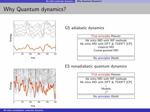
GS adiabatic dynamics
First principles Heaven
Ab initio MD with WF methodsAb initio MD with DFT & TDDFT [CP]
classical MDCoarse-grained MD
...
No principles World
ES nonadiabatic quantum dynamics
First principles Heaven
Ab initio MD with WF methodsAb initio MD with DFT & TDDFT [CP]
↓Models↓?
No principles World
Ab initio nonadiabatic molecular dynamics
Ab initio molecular dynamics Why Quantum Dynamics?
Why Quantum dynamics?E
nerg
y
Ene
rgy
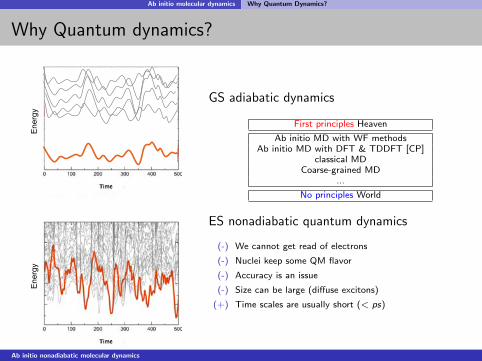
GS adiabatic dynamics
First principles Heaven
Ab initio MD with WF methodsAb initio MD with DFT & TDDFT [CP]
classical MDCoarse-grained MD
...
No principles World
ES nonadiabatic quantum dynamics
(-) We cannot get read of electrons
(-) Nuclei keep some QM flavor
(-) Accuracy is an issue
(-) Size can be large (diffuse excitons)
(+) Time scales are usually short (< ps)
Ab initio nonadiabatic molecular dynamics
Ab initio molecular dynamics Why Quantum Dynamics?
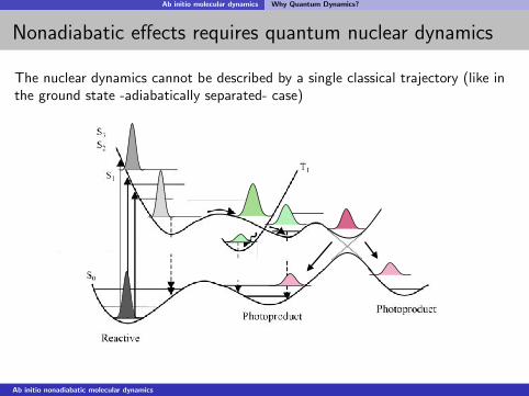
Nonadiabatic effects requires quantum nuclear dynamics
The nuclear dynamics cannot be described by a single classical trajectory (like inthe ground state -adiabatically separated- case)
Ab initio nonadiabatic molecular dynamics
Ab initio molecular dynamics Why Quantum Dynamics?
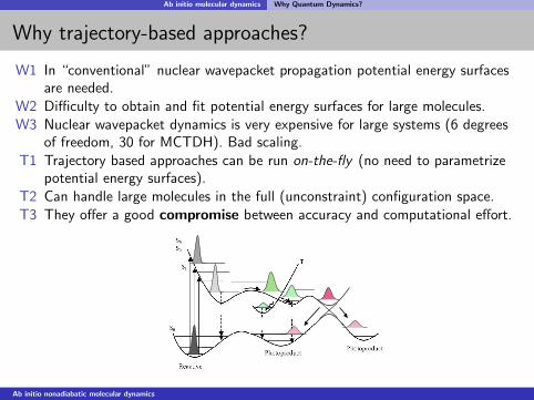
Why trajectory-based approaches?
W1 In “conventional” nuclear wavepacket propagation potential energy surfacesare needed.
W2 Difficulty to obtain and fit potential energy surfaces for large molecules.W3 Nuclear wavepacket dynamics is very expensive for large systems (6 degrees
of freedom, 30 for MCTDH). Bad scaling.T1 Trajectory based approaches can be run on-the-fly (no need to parametrize
potential energy surfaces).T2 Can handle large molecules in the full (unconstraint) configuration space.T3 They offer a good compromise between accuracy and computational effort.
Ab initio nonadiabatic molecular dynamics
Mixed quantum-classical dynamics
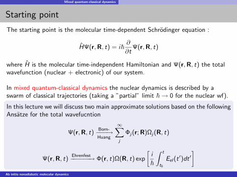
Starting point
The starting point is the molecular time-dependent Schrodinger equation :
HΨ(r,R, t) = i~∂
∂tΨ(r,R, t)
where H is the molecular time-independent Hamiltonian and Ψ(r,R, t) the totalwavefunction (nuclear + electronic) of our system.
In mixed quantum-classical dynamics the nuclear dynamics is described by aswarm of classical trajectories (taking a ”partial” limit ~→ 0 for the nuclear wf).
In this lecture we will discuss two main approximate solutions based on the followingAnsatze for the total wavefucntion
Ψ(r,R, t)Born-−−−→Huang
∞∑j
Φj(r; R)Ωj(R, t)
Ψ(r,R, t)Ehrenfest−−−−−−→ Φ(r, t)Ω(R, t) exp
[i
~
∫ t
t0
Eel(t ′)dt ′]
Ab initio nonadiabatic molecular dynamics
Mixed quantum-classical dynamics
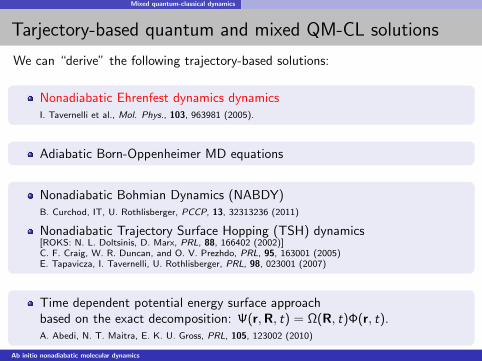
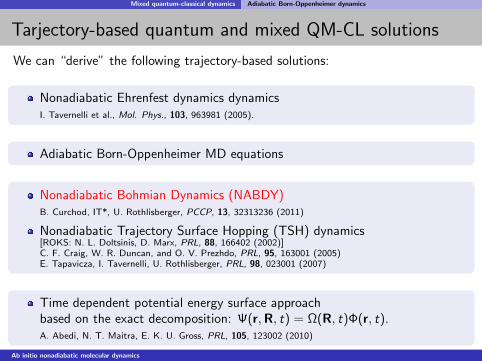
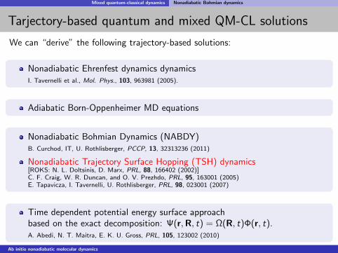
Tarjectory-based quantum and mixed QM-CL solutions
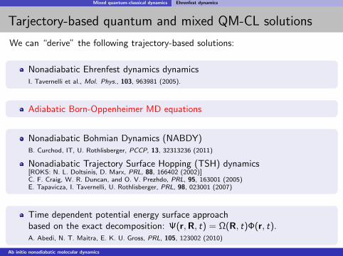
We can “derive” the following trajectory-based solutions:
Nonadiabatic Ehrenfest dynamics dynamicsI. Tavernelli et al., Mol. Phys., 103, 963981 (2005).
Adiabatic Born-Oppenheimer MD equations
Nonadiabatic Bohmian Dynamics (NABDY)B. Curchod, IT, U. Rothlisberger, PCCP, 13, 32313236 (2011)
Nonadiabatic Trajectory Surface Hopping (TSH) dynamics[ROKS: N. L. Doltsinis, D. Marx, PRL, 88, 166402 (2002)]C. F. Craig, W. R. Duncan, and O. V. Prezhdo, PRL, 95, 163001 (2005)E. Tapavicza, I. Tavernelli, U. Rothlisberger, PRL, 98, 023001 (2007)
Time dependent potential energy surface approachbased on the exact decomposition: Ψ(r,R, t) = Ω(R, t)Φ(r, t).A. Abedi, N. T. Maitra, E. K. U. Gross, PRL, 105, 123002 (2010)
Ab initio nonadiabatic molecular dynamics
Mixed quantum-classical dynamics Ehrenfest dynamics
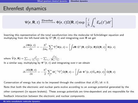
Ehrenfest dynamics
Ψ(r,R, t)Ehrenfest−−−−−−→ Φ(r, t)Ω(R, t) exp
[i
~
∫ t
t0
Eel(t ′)dt ′]
Inserting this representation of the total wavefunction into the molecular td Schrodinger equation andmultiplying from the left-hand side by Ω∗(R, t) and integrating over R we get
i~∂Φ(r, t)
∂t= −
~2
2me
Xi
∇2i Φ(r, t) +
»ZdR Ω∗(R, t)V (r,R)Ω(R, t)
–Φ(r, t)
where V (r,R) =P
i<je2
|ri−rj |−Pγ,i
e2Zγ|Rγ−ri |
.
In a similar way, multiplying by Φ∗(r, t) and integrating over r we obtain
i~∂Ω(R, t)
∂t= −
~2
2
Xγ
M−1γ ∇
2γΩ(R, t) +
»Zdr Φ∗(r, t)Hel Φ(r, t)
–Ω(R, t)
Conservation of energy has also to be imposed through the condition that d〈H〉/dt ≡ 0.
Note that both the electronic and nuclear parts evolve according to an average potential generated by the
other component (in square brakets). These average potentials are time-dependent and are responsible for the
feedback interaction between the electronic and nuclear components.
Ab initio nonadiabatic molecular dynamics
Mixed quantum-classical dynamics Ehrenfest dynamics
Ehrenfest dynamics - the nuclear equation
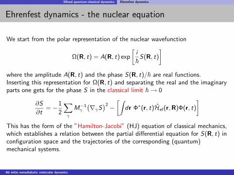
We start from the polar representation of the nuclear wavefunction
Ω(R, t) = A(R, t) exp
[i
~S(R, t)
]where the amplitude A(R, t) and the phase S(R, t)/~ are real functions.Inserting this representation for Ω(R, t) and separating the real and the imaginaryparts one gets for the phase S in the classical limit ~→ 0
∂S
∂t= −1
2
∑γ
M−1γ
(∇γS
)2 −[∫
dr Φ∗(r, t)Hel(r,R)Φ(r, t)
]This has the form of the ”Hamilton-Jacobi” (HJ) equation of classical mechanics,which establishes a relation between the partial differential equation for S(R, t) inconfiguration space and the trajectories of the corresponding (quantum)mechanical systems.
Ab initio nonadiabatic molecular dynamics
Mixed quantum-classical dynamics Ehrenfest dynamics
Ehrenfest dynamics - the nuclear equation
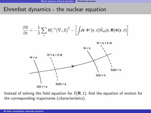
∂S
∂t= −1
2
∑γ
M−1γ
(∇γS
)2 −[∫
dr Φ∗(r, t)Hel(r,R)Φ(r, t)
]
Instead of solving the field equation for S(R, t), find the equation of motion forthe corresponding trajectories (characteristics).
Ab initio nonadiabatic molecular dynamics
Mixed quantum-classical dynamics Ehrenfest dynamics
Ehrenfest dynamics - the nuclear equation
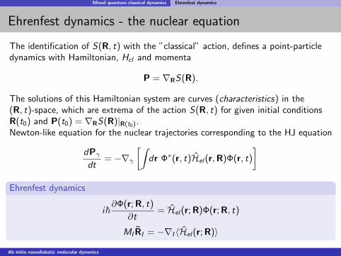
The identification of S(R, t) with the ”classical” action, defines a point-particledynamics with Hamiltonian, Hcl and momenta
P = ∇RS(R).
The solutions of this Hamiltonian system are curves (characteristics) in the(R, t)-space, which are extrema of the action S(R, t) for given initial conditionsR(t0) and P(t0) = ∇RS(R)|R(t0).Newton-like equation for the nuclear trajectories corresponding to the HJ equation
dPγdt
= −∇γ[∫
dr Φ∗(r, t)Hel(r,R)Φ(r, t)
]Ehrenfest dynamics
i~∂Φ(r; R, t)
∂t= Hel(r; R)Φ(r; R, t)
MI RI = −∇I 〈Hel(r; R)〉
Ab initio nonadiabatic molecular dynamics
Mixed quantum-classical dynamics Ehrenfest dynamics
Ehrenfest dynamics - the nuclear equation
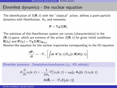
The identification of S(R, t) with the ”classical” action, defines a point-particledynamics with Hamiltonian, Hcl and momenta
P = ∇RS(R).
The solutions of this Hamiltonian system are curves (characteristics) in the(R, t)-space, which are extrema of the action S(R, t) for given initial conditionsR(t0) and P(t0) = ∇RS(R)|R(t0).Newton-like equation for the nuclear trajectories corresponding to the HJ equation
dPγdt
= −∇γ[∫
dr Φ∗(r, t)Hel(r,R)Φ(r, t)
]Ehrenfest dynamics - Densityfunctionalization (φk : KS orbitals)
i~∂
∂tφk(r, t) = − 1
2me∇2
rφk(r, t) + veff[ρ,Φ0](r, t)φk(r, t)
MI RI = −∇I E [ρ(r, t)]
Ab initio nonadiabatic molecular dynamics
Mixed quantum-classical dynamics Ehrenfest dynamics
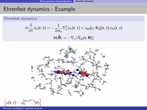
Ehrenfest dynamics - Example
Ehrenfest dynamics
i~∂
∂tφk(r, t) = − 1
2me∇2
rφk(r, t) + veff[ρ,Φ0](r, t)φk(r, t)
MI RI = −∇I 〈Hel(r; R)〉
[ρ(r, t)− ρ(no C4+)
0 (r)]
Ab initio nonadiabatic molecular dynamics
Mixed quantum-classical dynamics Ehrenfest dynamics
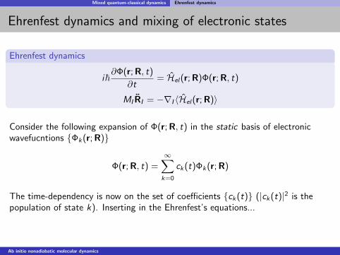
Ehrenfest dynamics and mixing of electronic states
Ehrenfest dynamics
i~∂Φ(r; R, t)
∂t= Hel(r; R)Φ(r; R, t)
MI RI = −∇I 〈Hel(r; R)〉
Consider the following expansion of Φ(r; R, t) in the static basis of electronicwavefucntions Φk(r; R)
Φ(r; R, t) =∞∑
k=0
ck(t)Φk(r; R)
The time-dependency is now on the set of coefficients ck(t) (|ck(t)|2 is thepopulation of state k). Inserting in the Ehrenfest’s equations...
Ab initio nonadiabatic molecular dynamics
Mixed quantum-classical dynamics Ehrenfest dynamics
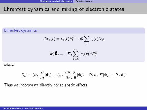
Ehrenfest dynamics and mixing of electronic states
Ehrenfest dynamics
i~ck(t) = ck(t)E elk − i~
∑j
cj(t)Dkj
MI RI = −∇I
∞∑k=0
|ck(t)|2E elk
where
Dkj = 〈Φk |∂
∂t|Φj〉 = 〈Φk |
∂R
∂t
∂
∂R|Φj〉 = R〈Φk |∇|Φj〉 = R · dkj
Thus we incorporate directly nonadiabatic effects.
Ab initio nonadiabatic molecular dynamics
Mixed quantum-classical dynamics Ehrenfest dynamics
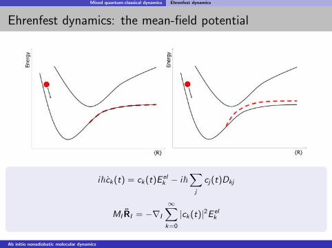
Ehrenfest dynamics: the mean-field potential
i~ck(t) = ck(t)E elk − i~
∑j
cj(t)Dkj
MI RI = −∇I
∞∑k=0
|ck(t)|2E elk
Ab initio nonadiabatic molecular dynamics
Mixed quantum-classical dynamics Ehrenfest dynamics
Tarjectory-based quantum and mixed QM-CL solutions
We can “derive” the following trajectory-based solutions:
Nonadiabatic Ehrenfest dynamics dynamicsI. Tavernelli et al., Mol. Phys., 103, 963981 (2005).
Adiabatic Born-Oppenheimer MD equations
Nonadiabatic Bohmian Dynamics (NABDY)B. Curchod, IT, U. Rothlisberger, PCCP, 13, 32313236 (2011)
Nonadiabatic Trajectory Surface Hopping (TSH) dynamics[ROKS: N. L. Doltsinis, D. Marx, PRL, 88, 166402 (2002)]C. F. Craig, W. R. Duncan, and O. V. Prezhdo, PRL, 95, 163001 (2005)E. Tapavicza, I. Tavernelli, U. Rothlisberger, PRL, 98, 023001 (2007)
Time dependent potential energy surface approachbased on the exact decomposition: Ψ(r,R, t) = Ω(R, t)Φ(r, t).A. Abedi, N. T. Maitra, E. K. U. Gross, PRL, 105, 123002 (2010)
Ab initio nonadiabatic molecular dynamics
Mixed quantum-classical dynamics Adiabatic Born-Oppenheimer dynamics
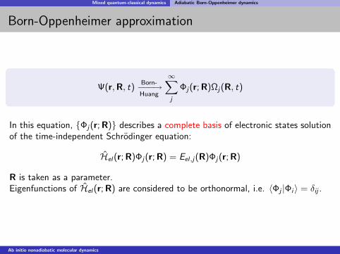
Born-Oppenheimer approximation
Ψ(r,R, t)Born-−−−→Huang
∞∑j
Φj(r; R)Ωj(R, t)
In this equation, Φj(r; R) describes a complete basis of electronic states solutionof the time-independent Schrodinger equation:
Hel(r; R)Φj(r; R) = Eel,j(R)Φj(r; R)
R is taken as a parameter.Eigenfunctions of Hel(r; R) are considered to be orthonormal, i.e. 〈Φj |Φi 〉 = δij .
Ab initio nonadiabatic molecular dynamics
Mixed quantum-classical dynamics Adiabatic Born-Oppenheimer dynamics
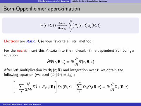
Born-Oppenheimer approximation
Ψ(r,R, t)Born-−−−→Huang
∞∑j
Φj(r; R)Ωj(R, t)
Electrons are static. Use your favorite el. str. method.
For the nuclei, insert this Ansatz into the molecular time-dependent Schrodingerequation
HΨ(r,R, t) = i~∂
∂tΨ(r,R, t)
After left multiplication by Φ∗k(r; R) and integration over r, we obtain thefollowing equation (we used 〈Φj |Φi 〉 = δij) :[
−∑
I
~2
2MI∇2
I + Eel,k(R)
]Ωk(R, t) +
∞∑j
DkjΩj(R, t) = i~∂
∂tΩk(R, t)
Ab initio nonadiabatic molecular dynamics
Mixed quantum-classical dynamics Adiabatic Born-Oppenheimer dynamics
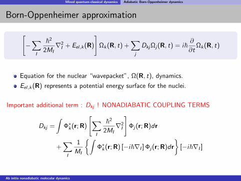
Born-Oppenheimer approximation
[−∑
I
~2
2MI∇2
I + Eel,k(R)
]Ωk(R, t) +
∑j
DkjΩj(R, t) = i~∂
∂tΩk(R, t)
Equation for the nuclear “wavepacket”, Ω(R, t), dynamics.
Eel,k(R) represents a potential energy surface for the nuclei.
Important additional term : Dkj ! NONADIABATIC COUPLING TERMS
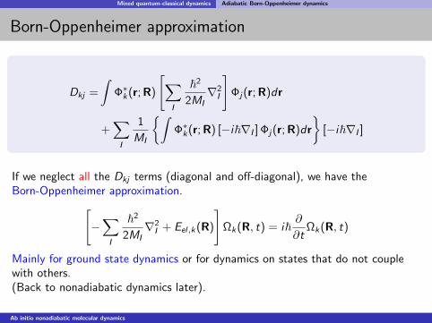
Dkj =
∫Φ∗k(r; R)
[∑I
~2
2MI∇2
I
]Φj(r; R)dr
+∑
I
1
MI
∫Φ∗k(r; R) [−i~∇I ] Φj(r; R)dr
[−i~∇I ]
Ab initio nonadiabatic molecular dynamics
Mixed quantum-classical dynamics Adiabatic Born-Oppenheimer dynamics
Born-Oppenheimer approximation
Dkj =
∫Φ∗k(r; R)
[∑I
~2
2MI∇2
I
]Φj(r; R)dr
+∑
I
1
MI
∫Φ∗k(r; R) [−i~∇I ] Φj(r; R)dr
[−i~∇I ]
If we neglect all the Dkj terms (diagonal and off-diagonal), we have theBorn-Oppenheimer approximation.[
−∑
I
~2
2MI∇2
I + Eel,k(R)
]Ωk(R, t) = i~
∂
∂tΩk(R, t)
Mainly for ground state dynamics or for dynamics on states that do not couplewith others.(Back to nonadiabatic dynamics later).
Ab initio nonadiabatic molecular dynamics
Mixed quantum-classical dynamics Adiabatic Born-Oppenheimer dynamics
Born-Oppenheimer approximation: the nuclear trajectories
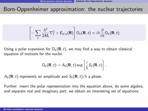
[−∑
I
~2
2MI∇2
I + Eel,k(R)
]Ωk(R, t) = i~
∂
∂tΩk(R, t)
Using a polar expansion for Ωk(R, t), we may find a way to obtain classicalequation of motions for the nuclei.
Ωk(R, t) = Ak(R, t) exp
[i
~Sk(R, t)
].
Ak(R, t) represents an amplitude and Sk(R, t)/~ a phase.
Further: insert the polar representation into the equation above, do some algebra,and separate real and imaginary part, we obtain an interesting set of equations:
Ab initio nonadiabatic molecular dynamics
Mixed quantum-classical dynamics Adiabatic Born-Oppenheimer dynamics
Born-Oppenheimer approximation: the nuclear trajectories
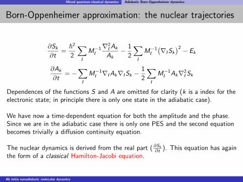
∂Sk
∂t=
~2
2
∑I
M−1I
∇2I Ak
Ak− 1
2
∑I
M−1I
(∇I Sk
)2 − Ek
∂Ak
∂t= −
∑I
M−1I ∇I Ak∇I Sk −
1
2
∑I
M−1I Ak∇2
I Sk
Dependences of the functions S and A are omitted for clarity (k is a index for theelectronic state; in principle there is only one state in the adiabatic case).
We have now a time-dependent equation for both the amplitude and the phase.Since we are in the adiabatic case there is only one PES and the second equationbecomes trivially a diffusion continuity equation.
The nuclear dynamics is derived from the real part (∂Sk
∂t ). This equation has againthe form of a classical Hamilton-Jacobi equation.
Ab initio nonadiabatic molecular dynamics
Mixed quantum-classical dynamics Adiabatic Born-Oppenheimer dynamics
Born-Oppenheimer approximation: the nuclear trajectories
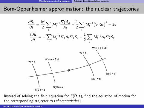
∂Sk
∂t=
~2
2
∑I
M−1I
∇2I Ak
Ak− 1
2
∑I
M−1I
(∇I Sk
)2 − Ek
∂Ak
∂t= −
∑I
M−1I ∇I Ak∇I Sk −
1
2
∑I
M−1I Ak∇2
I Sk
Instead of solving the field equation for S(R, t), find the equation of motion forthe corresponding trajectories (characteristics).
Ab initio nonadiabatic molecular dynamics
Mixed quantum-classical dynamics Adiabatic Born-Oppenheimer dynamics
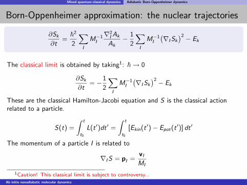
Born-Oppenheimer approximation: the nuclear trajectories
∂Sk
∂t=
~2
2
∑I
M−1I
∇2I Ak
Ak− 1
2
∑I
M−1I
(∇I Sk
)2 − Ek
The classical limit is obtained by taking1: ~→ 0
∂Sk
∂t= −1
2
∑I
M−1I
(∇I Sk
)2 − Ek
These are the classical Hamilton-Jacobi equation and S is the classical actionrelated to a particle.
S(t) =
∫ t
t0
L(t ′)dt ′ =
∫ t
t0
[Ekin(t ′)− Epot(t ′)] dt ′
The momentum of a particle I is related to
∇I S = pI =vI
MI
1Caution! This classical limit is subject to controversy...Ab initio nonadiabatic molecular dynamics
Mixed quantum-classical dynamics Adiabatic Born-Oppenheimer dynamics
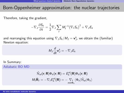
Born-Oppenheimer approximation: the nuclear trajectories
Therefore, taking the gradient,
−∇J∂Sk
∂t=
1
2∇J
∑I
M−1I
(∇I Sk
)2+∇JEk
and rearranging this equation using ∇JSk/MJ = vkJ , we obtain the (familiar)
Newton equation:
MJd
dtvk
J = −∇JEk
In Summary:
Adiabatic BO MD
Hel(r; R)Φk(r; R) = E elk (R)Φk(r; R)
MI RI = −∇I Eelk (R) = − ∇I
minΦk
〈Φk |Hel |Φk〉
Ab initio nonadiabatic molecular dynamics
Mixed quantum-classical dynamics Adiabatic Born-Oppenheimer dynamics
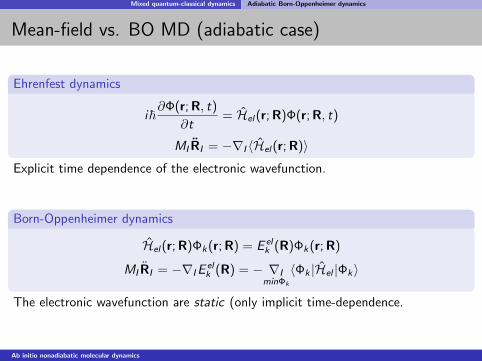
Mean-field vs. BO MD (adiabatic case)
Ehrenfest dynamics
i~∂Φ(r; R, t)
∂t= Hel(r; R)Φ(r; R, t)
MI RI = −∇I 〈Hel(r; R)〉Explicit time dependence of the electronic wavefunction.
Born-Oppenheimer dynamics
Hel(r; R)Φk(r; R) = E elk (R)Φk(r; R)
MI RI = −∇I Eelk (R) = − ∇I
minΦk
〈Φk |Hel |Φk〉
The electronic wavefunction are static (only implicit time-dependence.
Ab initio nonadiabatic molecular dynamics
Mixed quantum-classical dynamics Adiabatic Born-Oppenheimer dynamics
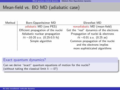
Mean-field vs. BO MD (adiabatic case)
Method Born-Oppenheimer MD Ehrenfest MD
adiabatic MD (one PES) nonadiabatic MD (mean-field)Efficient propagation of the nuclei Get the “real” dynamics of the electrons
Adiabatic nuclear propagation Propagation of nuclei & electronsδt ∼10-20 a.u. (0.25-0.5 fs) δt ∼0.01 a.u. (0.25 as)
Simple algorithm Common propagation of the nucleiand the electrons implies
more sophisticated algorithms
Exact quantum dynamics?Can we derive “exact” quantum equations of motion for the nuclei?(without taking the classical limit ~→ 0?)
Ab initio nonadiabatic molecular dynamics
Mixed quantum-classical dynamics Adiabatic Born-Oppenheimer dynamics
Tarjectory-based quantum and mixed QM-CL solutions
We can “derive” the following trajectory-based solutions:
Nonadiabatic Ehrenfest dynamics dynamicsI. Tavernelli et al., Mol. Phys., 103, 963981 (2005).
Adiabatic Born-Oppenheimer MD equations
Nonadiabatic Bohmian Dynamics (NABDY)B. Curchod, IT*, U. Rothlisberger, PCCP, 13, 32313236 (2011)
Nonadiabatic Trajectory Surface Hopping (TSH) dynamics[ROKS: N. L. Doltsinis, D. Marx, PRL, 88, 166402 (2002)]C. F. Craig, W. R. Duncan, and O. V. Prezhdo, PRL, 95, 163001 (2005)E. Tapavicza, I. Tavernelli, U. Rothlisberger, PRL, 98, 023001 (2007)
Time dependent potential energy surface approachbased on the exact decomposition: Ψ(r,R, t) = Ω(R, t)Φ(r, t).A. Abedi, N. T. Maitra, E. K. U. Gross, PRL, 105, 123002 (2010)
Ab initio nonadiabatic molecular dynamics
Mixed quantum-classical dynamics Adiabatic Born-Oppenheimer dynamics
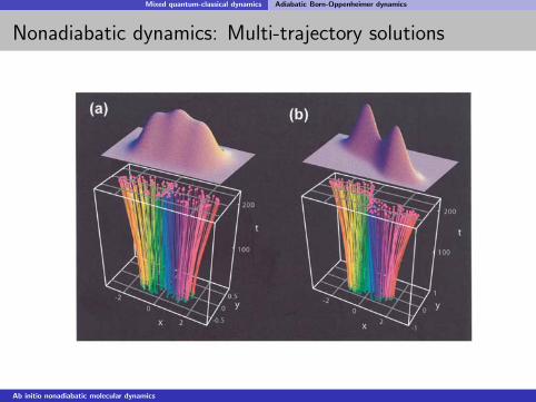
Nonadiabatic dynamics: Multi-trajectory solutions
Ab initio nonadiabatic molecular dynamics
Mixed quantum-classical dynamics Nonadiabatic Bohmian dynamics
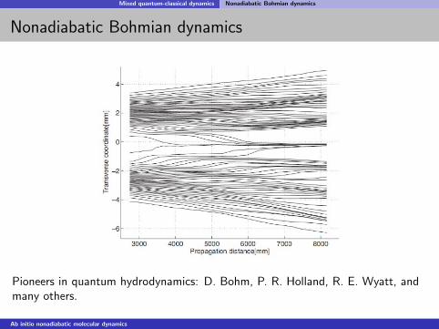
Nonadiabatic Bohmian dynamics
Pioneers in quantum hydrodynamics: D. Bohm, P. R. Holland, R. E. Wyatt, andmany others.
Ab initio nonadiabatic molecular dynamics
Mixed quantum-classical dynamics Nonadiabatic Bohmian dynamics
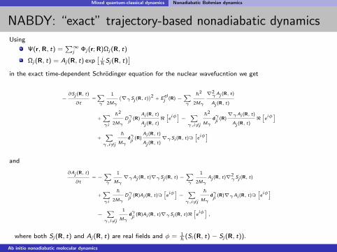
NABDY: “exact” trajectory-based nonadiabatic dynamicsUsing
Ψ(r,R, t) =P∞
j Φj (r; R)Ωj (R, t)
Ωj (R, t) = Aj (R, t) expˆ
i~ Sj (R, t)
˜in the exact time-dependent Schrodinger equation for the nuclear wavefucntion we get
−∂Sj (R, t)
∂t=Xγ
1
2Mγ
`∇γSj (R, t)
´2 + Eelj (R) −
Xγ
~2
2Mγ
∇2γAj (R, t)
Aj (R, t)
+Xγi
~2
2MγDγji
(R)Ai (R, t)
Aj (R, t)<heiφ
i−
Xγ,i 6=j
~2
Mγdγji
(R)∇γAi (R, t)
Aj (R, t)<heiφ
i
+Xγ,i 6=j
~
Mγdγji
(R)Ai (R, t)
Aj (R, t)∇γSi (R, t)=
heiφ
i
and
∂Aj (R, t)
∂t= −
Xγ
1
Mγ∇γAj (R, t)∇γSj (R, t) −
Xγ
1
2MγAj (R, t)∇2
γSj (R, t)
+Xγi
~
2MγDγji
(R)Ai (R, t)=heiφ
i−
Xγ,i 6=j
~
Mγdγji
(R)∇γAi (R, t)=heiφ
i
−Xγ,i 6=j
1
Mγdγji
(R)Ai (R, t)∇γSi (R, t)<heiφ
i,
where both Sj (R, t) and Aj (R, t) are real fields and φ = 1~ (Si (R, t)− Sj (R, t)).
Ab initio nonadiabatic molecular dynamics
Mixed quantum-classical dynamics Nonadiabatic Bohmian dynamics
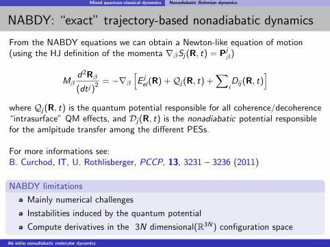
NABDY: “exact” trajectory-based nonadiabatic dynamics
From the NABDY equations we can obtain a Newton-like equation of motion(using the HJ definition of the momenta ∇βSj(R, t) = Pj
β)
Mβd2Rβ
(dt j)2 = −∇β
[E j
el(R) +Qj(R, t) +∑
iDij(R, t)
]where Qj(R, t) is the quantum potential responsible for all coherence/decoherence“intrasurface” QM effects, and Dj(R, t) is the nonadiabatic potential responsiblefor the amlpitude transfer among the different PESs.
For more informations see:B. Curchod, IT, U. Rothlisberger, PCCP, 13, 3231 – 3236 (2011)
NABDY limitations
Mainly numerical challenges
Instabilities induced by the quantum potential
Compute derivatives in the 3N dimensional(R3N) configuration space
Ab initio nonadiabatic molecular dynamics
Mixed quantum-classical dynamics Nonadiabatic Bohmian dynamics
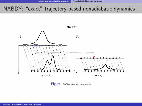
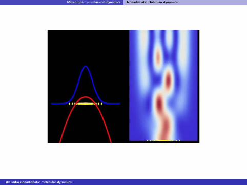
NABDY: “exact” trajectory-based nonadiabatic dynamics
Figure: NABDY: sketch of the dynamics
Ab initio nonadiabatic molecular dynamics
Mixed quantum-classical dynamics Nonadiabatic Bohmian dynamics
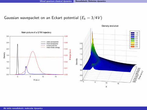
Gaussian wavepacket on an Eckart potential (Ek = 3/4V )
Ab initio nonadiabatic molecular dynamics
Mixed quantum-classical dynamics Nonadiabatic Bohmian dynamics
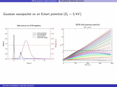
Gaussian wavepacket on an Eckart potential (Ek = 3/4V )
Ab initio nonadiabatic molecular dynamics
Mixed quantum-classical dynamics Nonadiabatic Bohmian dynamics
Ab initio nonadiabatic molecular dynamics
Mixed quantum-classical dynamics Nonadiabatic Bohmian dynamics
Tarjectory-based quantum and mixed QM-CL solutions
We can “derive” the following trajectory-based solutions:
Nonadiabatic Ehrenfest dynamics dynamicsI. Tavernelli et al., Mol. Phys., 103, 963981 (2005).
Adiabatic Born-Oppenheimer MD equations
Nonadiabatic Bohmian Dynamics (NABDY)B. Curchod, IT, U. Rothlisberger, PCCP, 13, 32313236 (2011)
Nonadiabatic Trajectory Surface Hopping (TSH) dynamics[ROKS: N. L. Doltsinis, D. Marx, PRL, 88, 166402 (2002)]C. F. Craig, W. R. Duncan, and O. V. Prezhdo, PRL, 95, 163001 (2005)E. Tapavicza, I. Tavernelli, U. Rothlisberger, PRL, 98, 023001 (2007)
Time dependent potential energy surface approachbased on the exact decomposition: Ψ(r,R, t) = Ω(R, t)Φ(r, t).A. Abedi, N. T. Maitra, E. K. U. Gross, PRL, 105, 123002 (2010)
Ab initio nonadiabatic molecular dynamics

Mixed quantum-classical dynamics Trajectory Surface Hopping
Applications in Photochemistry and Photophysics
Trajectory-based solutions of the “exact” nonadiabatic equations are stillimpractical.
Approximate solutions are available. Among the most popular is
Trajectory Surface Hopping (TSH)
Ab initio nonadiabatic molecular dynamics
Mixed quantum-classical dynamics Trajectory Surface Hopping
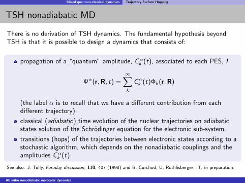
TSH nonadiabatic MD
There is no derivation of TSH dynamics. The fundamental hypothesis beyondTSH is that it is possible to design a dynamics that consists of:
propagation of a “quantum” amplitude, Cαk (t), associated to each PES, I
Ψα(r,R, t) =∞∑k
Cαk (t)Φk(r; R)
(the label α is to recall that we have a different contribution from eachdifferent trajectory).
classical (adiabatic) time evolution of the nuclear trajectories on adiabaticstates solution of the Schrodinger equation for the electronic sub-system.
transitions (hops) of the trajectories between electronic states according to astochastic algorithm, which depends on the nonadiabatic couplings and theamplitudes Cα
k (t).
See also: J. Tully, Faraday discussion, 110, 407 (1998) and B. Curchod, U. Rothlisberger, IT, in preparation.
Ab initio nonadiabatic molecular dynamics
Mixed quantum-classical dynamics Trajectory Surface Hopping
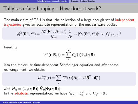
Tully’s surface hopping - How does it work?
The main claim of TSH is that, the collection of a large enough set of independenttrajectories gives an accurate representation of the nuclear wave packet
ρCLk (Rα, tα) =
Nαk (Rα, dV , tα)
Ntot
1
dV∼ |Ωk(Rα, tα)|2 ∼ |Cα
k,Rα,tα |2
Inserting
Ψα(r,R, t) =∞∑k
Cαk (t)Φk(r; R)
into the molecular time-dependent Schrodinger equation and after somerearrangement, we obtain:
i~Cαk (t) =
∑j
Cαj (t)(Hkj − i~R
α · dαkj)
with Hkj = 〈Φk(r; R)〉|Hel |Φj(r; R)〉.In the adiabatic representation, we have Hkk = E el
k and Hkj = 0 .
Ab initio nonadiabatic molecular dynamics
Mixed quantum-classical dynamics Trajectory Surface Hopping
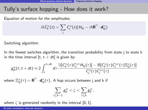
Tully’s surface hopping - How does it work?
Equation of motion for the amplitudes:
i~Cαk (t) =
∑j
Cαj (t)(Hkj − i~R
α · dαkj)
Switching algorithm:
In the fewest switches algorithm, the transition probability from state j to state kin the time interval [t, t + dt] is given by:
gαjk (t, t + dt) ≈ 2
∫ t+dt
t
dτ=[Cα
k (τ)Cα∗j Hkj(τ)]−<[Cα
k (τ)Cα∗j (τ)Ξαkj(τ)]
Cαj (τ)Cα∗
j (τ)
where Ξαkj(τ) = Rα · dαkj(τ). A hop occurs between j and k if∑
l≤k−1
gαjl < ζ <∑l≤k
gαjl ,
where ζ is generated randomly in the interval [0, 1].Ab initio nonadiabatic molecular dynamics

Mixed quantum-classical dynamics Trajectory Surface Hopping
Tully’s surface hopping - Summary
Tully’s surface hopping
i~Cαk (t) =
∑j
Cαj (t)(Hkj − i~R
α · dαkj)
MI RI = −∇I Eelk (R)∑
l≤k−1
gαjl < ζ <∑l≤k
gαjl ,
Some warnings:
1 Evolution of classical trajectories (no QM effects – such as tunneling – arepossible).
2 Rescaling of the nuclei velocities after a surface hop (to ensure energyconservation) is still a matter of debate.
3 Depending on the system studied, many trajectories could be needed toobtain a complete statistical description of the non-radiative channels.
For more details (and warnings) about Tully’s surface hopping, see G. Granucci and M. Persico,
J Chem Phys 126, 134114 (2007).
Ab initio nonadiabatic molecular dynamics
Mixed quantum-classical dynamics Trajectory Surface Hopping
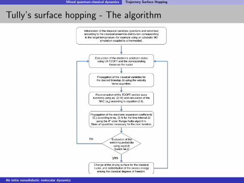
Tully’s surface hopping - The algorithm
Ab initio nonadiabatic molecular dynamics
Mixed quantum-classical dynamics Trajectory Surface Hopping
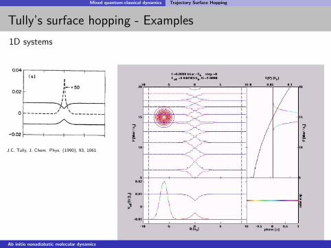
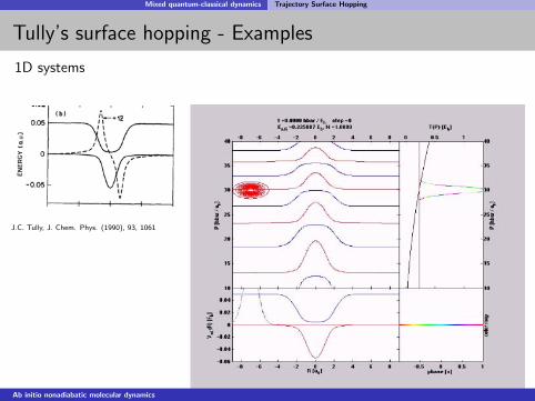
Tully’s surface hopping - Examples
1D systems
J.C. Tully, J. Chem. Phys. (1990), 93, 1061
Very good agreement with exact nuclear wavepacket propagation.
Ab initio nonadiabatic molecular dynamics
Mixed quantum-classical dynamics Trajectory Surface Hopping
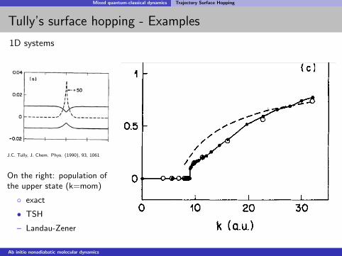
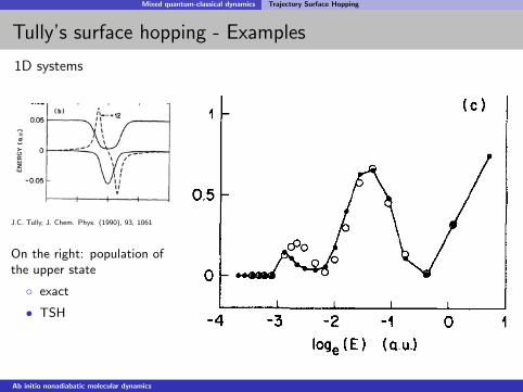
Tully’s surface hopping - Examples
1D systems
J.C. Tully, J. Chem. Phys. (1990), 93, 1061
On the right: population ofthe upper state (k=mom)
exact
• TSH
– Landau-Zener
Very good agreement with exact nuclear wavepacket propagation.
Ab initio nonadiabatic molecular dynamics
Mixed quantum-classical dynamics Trajectory Surface Hopping
Tully’s surface hopping - Examples
1D systems
J.C. Tully, J. Chem. Phys. (1990), 93, 1061
Very good agreement with exact nuclear wavepacket propagation.
Ab initio nonadiabatic molecular dynamics
Mixed quantum-classical dynamics Trajectory Surface Hopping
Tully’s surface hopping - Examples
1D systems
J.C. Tully, J. Chem. Phys. (1990), 93, 1061
On the right: population ofthe upper state
exact
• TSH
Very good agreement with exact nuclear wavepacket propagation.
Ab initio nonadiabatic molecular dynamics
Mixed quantum-classical dynamics Trajectory Surface Hopping
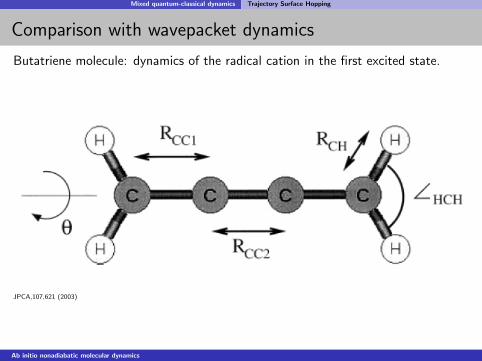
Comparison with wavepacket dynamics
Butatriene molecule: dynamics of the radical cation in the first excited state.
JPCA,107,621 (2003)
Ab initio nonadiabatic molecular dynamics
Mixed quantum-classical dynamics Trajectory Surface Hopping
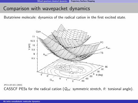
Comparison with wavepacket dynamics
Butatriene molecule: dynamics of the radical cation in the first excited state.
JPCA,107,621 (2003)
CASSCF PESs for the radical cation (Q14: symmetric stretch, θ: torsional angle).
Ab initio nonadiabatic molecular dynamics
Mixed quantum-classical dynamics Trajectory Surface Hopping
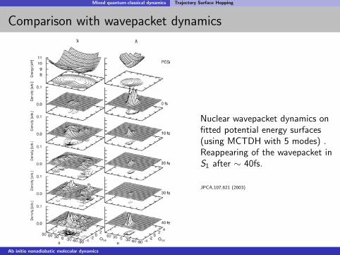
Comparison with wavepacket dynamics
Nuclear wavepacket dynamics onfitted potential energy surfaces(using MCTDH with 5 modes) .Reappearing of the wavepacket inS1 after ∼ 40fs.
JPCA,107,621 (2003)
Ab initio nonadiabatic molecular dynamics
Mixed quantum-classical dynamics Trajectory Surface Hopping
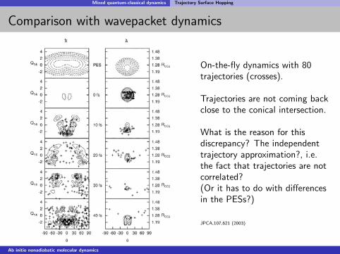
Comparison with wavepacket dynamics
On-the-fly dynamics with 80trajectories (crosses).
Trajectories are not coming backclose to the conical intersection.
What is the reason for thisdiscrepancy? The independenttrajectory approximation?, i.e.the fact that trajectories are notcorrelated?(Or it has to do with differencesin the PESs?)
JPCA,107,621 (2003)
Ab initio nonadiabatic molecular dynamics
Mixed quantum-classical dynamics Trajectory Surface Hopping
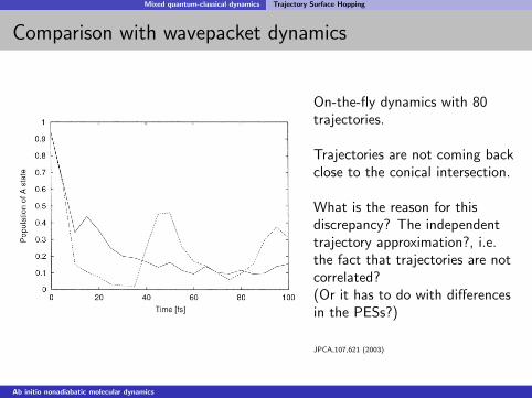
Comparison with wavepacket dynamics
On-the-fly dynamics with 80trajectories.
Trajectories are not coming backclose to the conical intersection.
What is the reason for thisdiscrepancy? The independenttrajectory approximation?, i.e.the fact that trajectories are notcorrelated?(Or it has to do with differencesin the PESs?)
JPCA,107,621 (2003)
Ab initio nonadiabatic molecular dynamics
TDDFT-based trajectory surface hopping
1 Ab initio molecular dynamicsWhy Quantum Dynamics?
2 Mixed quantum-classical dynamicsEhrenfest dynamicsAdiabatic Born-Oppenheimer dynamicsNonadiabatic Bohmian dynamicsTrajectory Surface Hopping
3 TDDFT-based trajectory surface hoppingNonadiabatic couplings in TDDFT
4 TDDFT-TSH: ApplicationsPhotodissociation of OxiraneOxirane - Crossing between S1 and S0
5 TSH with external time-dependent fields
Ab initio nonadiabatic molecular dynamics
TDDFT-based trajectory surface hopping
Tully’s surface hopping - On-the-fly dynamics
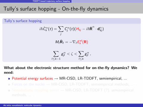
Tully’s surface hopping
i~Cαk (t) =
∑j
Cαj (t)(Hkj − i~R
α · dαkj)
MI RI = −∇I Eelk (R)
∑l≤k−1
gαjl < ζ <∑l≤k
gαjl ,
What about the electronic structure method for on-the-fly dynamics? Weneed:
Potential energy surfaces → MR-CISD, LR-TDDFT, semiempirical, ...
Forces on the nuclei → MR-CISD, LR-TDDFT, semiempirical methods, ... .
Nonadiabatic coupling terms → MR-CISD, LR-TDDFT (?), semiempiricalmethods, ... .
Ab initio nonadiabatic molecular dynamics
TDDFT-based trajectory surface hopping
Tully’s surface hopping - On-the-fly dynamics
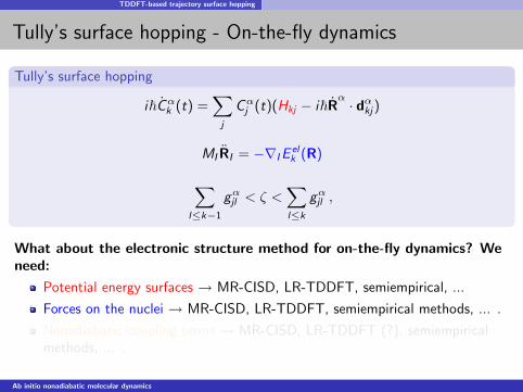
Tully’s surface hopping
i~Cαk (t) =
∑j
Cαj (t)(Hkj − i~R
α · dαkj)
MI RI = −∇I Eelk (R)
∑l≤k−1
gαjl < ζ <∑l≤k
gαjl ,
What about the electronic structure method for on-the-fly dynamics? Weneed:
Potential energy surfaces → MR-CISD, LR-TDDFT, semiempirical, ...
Forces on the nuclei → MR-CISD, LR-TDDFT, semiempirical methods, ... .
Nonadiabatic coupling terms → MR-CISD, LR-TDDFT (?), semiempiricalmethods, ... .
Ab initio nonadiabatic molecular dynamics
TDDFT-based trajectory surface hopping
Tully’s surface hopping - On-the-fly dynamics
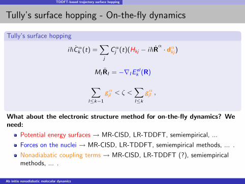
Tully’s surface hopping
i~Cαk (t) =
∑j
Cαj (t)(Hkj − i~R
α · dαkj)
MI RI = −∇I Eelk (R)
∑l≤k−1
gαjl < ζ <∑l≤k
gαjl ,
What about the electronic structure method for on-the-fly dynamics? Weneed:
Potential energy surfaces → MR-CISD, LR-TDDFT, semiempirical, ...
Forces on the nuclei → MR-CISD, LR-TDDFT, semiempirical methods, ... .
Nonadiabatic coupling terms → MR-CISD, LR-TDDFT (?), semiempiricalmethods, ... .
Ab initio nonadiabatic molecular dynamics
TDDFT-based trajectory surface hopping Nonadiabatic couplings in TDDFT
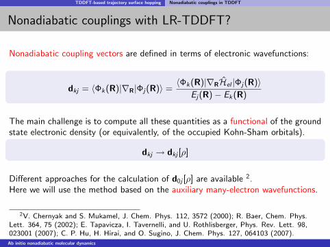
Nonadiabatic couplings with LR-TDDFT?
Nonadiabatic coupling vectors are defined in terms of electronic wavefunctions:
dkj = 〈Φk(R)|∇R|Φj(R)〉 =〈Φk(R)|∇RHel |Φj(R)〉
Ej(R)− Ek(R)
The main challenge is to compute all these quantities as a functional of the groundstate electronic density (or equivalently, of the occupied Kohn-Sham orbitals).
dkj → dkj [ρ]
Different approaches for the calculation of d0j [ρ] are available 2.Here we will use the method based on the auxiliary many-electron wavefunctions.
2V. Chernyak and S. Mukamel, J. Chem. Phys. 112, 3572 (2000); R. Baer, Chem. Phys.Lett. 364, 75 (2002); E. Tapavicza, I. Tavernelli, and U. Rothlisberger, Phys. Rev. Lett. 98,023001 (2007); C. P. Hu, H. Hirai, and O. Sugino, J. Chem. Phys. 127, 064103 (2007).
Ab initio nonadiabatic molecular dynamics
TDDFT-based trajectory surface hopping Nonadiabatic couplings in TDDFT
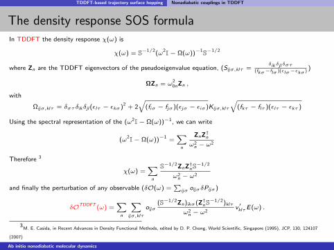
The density response SOS formulaIn TDDFT the density response χ(ω) is
χ(ω) = S−1/2(ω2I− Ω(ω))−1S−1/2
where Zn are the TDDFT eigenvectors of the pseudoeigenvalue equation, (Sijσ,klτ =δikδjlδστ
(fkσ−flσ )(εlσ−εkσ ) )
ΩZn = ω20nZn ,
with
Ωijσ,klτ = δστδikδjl (εlτ − εkσ)2 + 2q
(fiσ − fjσ)(εjσ − εiσ)Kijσ,klτ
q(fkτ − flτ )(εlτ − εkτ )
Using the spectral representation of the (ω2I− Ω(ω))−1, we can write
(ω2I− Ω(ω))−1 =X
n
ZnZ†nω2
n − ω2
Therefore 3
χ(ω) =X
n
S−1/2ZnZ†n S−1/2
ω2n − ω2
and finally the perturbation of any observable (δO(ω) =P
ijσ oijσδPijσ)
δOTDDFT (ω) =X
n
Xijσ,klτ
oijσ(S−1/2Zn)ikσ(Z†n S−1/2)klτ
ω2n − ω2
v ′klτE(ω) .
3M. E. Casida, in Recent Advances in Density Functional Methods, edited by D. P. Chong, World Scientific, Singapore (1995), JCP, 130, 124107
(2007)
Ab initio nonadiabatic molecular dynamics
TDDFT-based trajectory surface hopping Nonadiabatic couplings in TDDFT
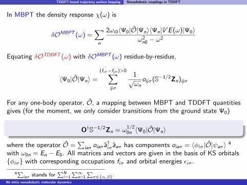
In MBPT the density response χ(ω) is
δOMBPT (ω) =∑
n
2ωi0〈Ψ0|O|Ψn〉〈Ψn|v ′E (ω)|Ψ0〉ω2
n0 − ω2
Equating δOTDDFT (ω) with δOMBPT (ω) residue-by-residue,
〈Ψ0|O|Ψn〉 =
(fiσ−fjσ)>0∑ijσ
1√ωn
oijσ(S−1/2Zn)ijσ
For any one-body operator, O, a mapping between MBPT and TDDFT quantitiesgives (for the moment, we only consider transitions from the ground state Ψ0)
O†S−1/2Zn = ω1/20n 〈Ψ0|O|Ψn〉
where the operator O =∑
iaσ oiaσ a†iσ aaσ has components oiaσ = 〈φiσ|O|ψaσ〉 4
with ω0n = En − E0. All matrices and vectors are given in the basis of KS orbitalsφiσ with corresponding occupations fiσ and orbital energies εiσ.
4P
iaσ stands forPN
i=1
P∞a=1
Pσ∈α,β.
Ab initio nonadiabatic molecular dynamics
TDDFT-based trajectory surface hopping Nonadiabatic couplings in TDDFT
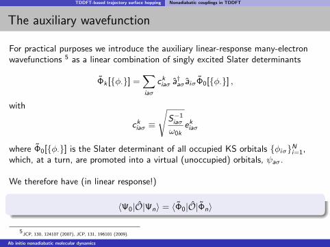
The auxiliary wavefunction
For practical purposes we introduce the auxiliary linear-response many-electronwavefunctions 5 as a linear combination of singly excited Slater determinants
Φk [φ·] =∑iaσ
ckiaσ a†aσ aiσΦ0[φ·] ,
with
ckiaσ ≡
√S−1
iaσ
ω0kekiaσ
where Φ0[φ·] is the Slater determinant of all occupied KS orbitals φiσNi=1,which, at a turn, are promoted into a virtual (unoccupied) orbitals, ψaσ.
We therefore have (in linear response!)
〈Ψ0|O|Ψn〉 = 〈Φ0|O|Φn〉
5JCP, 130, 124107 (2007), JCP, 131, 196101 (2009).
Ab initio nonadiabatic molecular dynamics
TDDFT-based trajectory surface hopping Nonadiabatic couplings in TDDFT
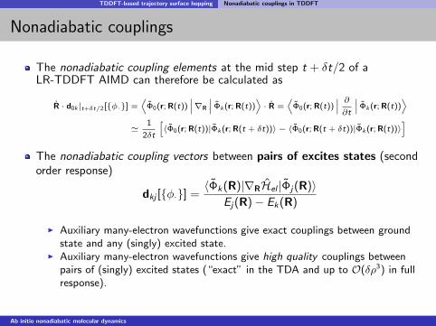
Nonadiabatic couplings
The nonadiabatic coupling elements at the mid step t + δt/2 of aLR-TDDFT AIMD can therefore be calculated as
R · d0k |t+δt/2[φ·] =D
Φ0(r; R(t))˛∇R
˛Φk (r; R(t))
E· R =
DΦ0(r; R(t))
˛ ∂∂t
˛Φk (r; R(t))
E'
1
2δt
h〈Φ0(r; R(t))|Φk (r; R(t + δt))〉 − 〈Φ0(r; R(t + δt))|Φk (r; R(t))〉
iThe nonadiabatic coupling vectors between pairs of excites states (secondorder response)
dkj [φ·] =〈Φk(R)|∇RHel |Φj(R)〉
Ej(R)− Ek(R)
I Auxiliary many-electron wavefunctions give exact couplings between groundstate and any (singly) excited state.
I Auxiliary many-electron wavefunctions give high quality couplings betweenpairs of (singly) excited states (“exact” in the TDA and up to O(δρ3) in fullresponse).
Ab initio nonadiabatic molecular dynamics
TDDFT-based trajectory surface hopping Nonadiabatic couplings in TDDFT
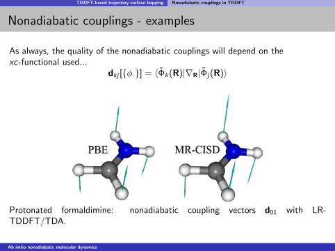
Nonadiabatic couplings - examples
As always, the quality of the nonadiabatic couplings will depend on thexc-functional used...
dkj [φ·] = 〈Φk(R)|∇R|Φj(R)〉
Protonated formaldimine: nonadiabatic coupling vectors d01 with LR-TDDFT/TDA.
Ab initio nonadiabatic molecular dynamics
TDDFT-based trajectory surface hopping Nonadiabatic couplings in TDDFT
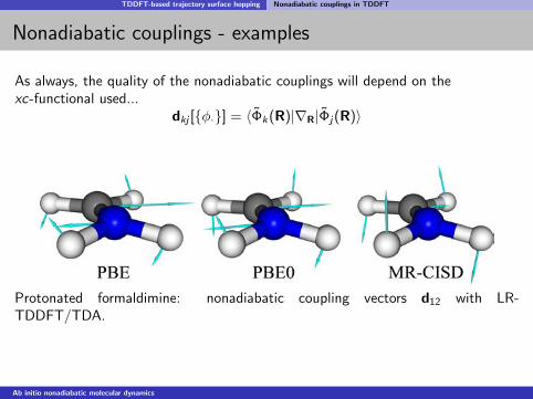
Nonadiabatic couplings - examples
As always, the quality of the nonadiabatic couplings will depend on thexc-functional used...
dkj [φ·] = 〈Φk(R)|∇R|Φj(R)〉
Protonated formaldimine: nonadiabatic coupling vectors d12 with LR-TDDFT/TDA.
Ab initio nonadiabatic molecular dynamics
TDDFT-TSH: Applications
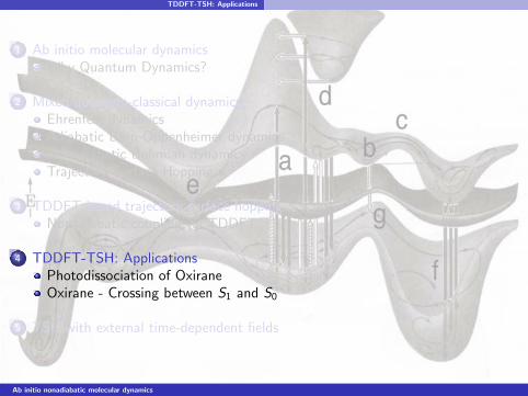
1 Ab initio molecular dynamicsWhy Quantum Dynamics?
2 Mixed quantum-classical dynamicsEhrenfest dynamicsAdiabatic Born-Oppenheimer dynamicsNonadiabatic Bohmian dynamicsTrajectory Surface Hopping
3 TDDFT-based trajectory surface hoppingNonadiabatic couplings in TDDFT
4 TDDFT-TSH: ApplicationsPhotodissociation of OxiraneOxirane - Crossing between S1 and S0
5 TSH with external time-dependent fields
Ab initio nonadiabatic molecular dynamics
TDDFT-TSH: Applications
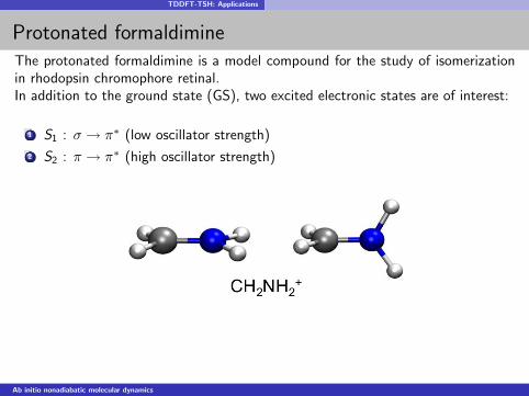
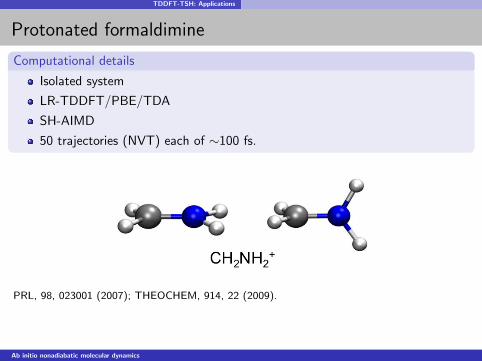
Protonated formaldimineThe protonated formaldimine is a model compound for the study of isomerizationin rhodopsin chromophore retinal.In addition to the ground state (GS), two excited electronic states are of interest:
1 S1 : σ → π∗ (low oscillator strength)
2 S2 : π → π∗ (high oscillator strength)
Ab initio nonadiabatic molecular dynamics
TDDFT-TSH: Applications
Protonated formaldimine
Computational details
Isolated system
LR-TDDFT/PBE/TDA
SH-AIMD
50 trajectories (NVT) each of ∼100 fs.
PRL, 98, 023001 (2007); THEOCHEM, 914, 22 (2009).
Ab initio nonadiabatic molecular dynamics
TDDFT-TSH: Applications
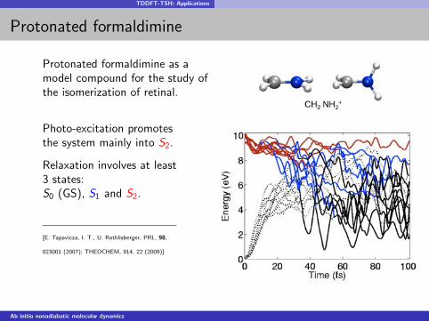
Protonated formaldimine
Protonated formaldimine as amodel compound for the study ofthe isomerization of retinal.
Photo-excitation promotesthe system mainly into S2.
Relaxation involves at least3 states:S0 (GS), S1 and S2.
[E. Tapavicza, I. T., U. Rothlisberger, PRL, 98,
023001 (2007); THEOCHEM, 914, 22 (2009)]
Ab initio nonadiabatic molecular dynamics
TDDFT-TSH: Applications
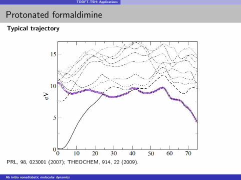
Protonated formaldimine
Typical trajectory
PRL, 98, 023001 (2007); THEOCHEM, 914, 22 (2009).
Ab initio nonadiabatic molecular dynamics
TDDFT-TSH: Applications
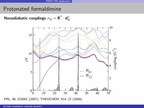
Protonated formaldimine
Nonadiabatic couplings σkj = Rα · dαkj
PRL, 98, 023001 (2007); THEOCHEM, 914, 22 (2009).
Ab initio nonadiabatic molecular dynamics
TDDFT-TSH: Applications
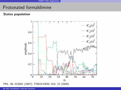
Protonated formaldimine
States population
PRL, 98, 023001 (2007); THEOCHEM, 914, 22 (2009).
Ab initio nonadiabatic molecular dynamics
TDDFT-TSH: Applications
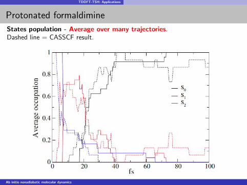
Protonated formaldimine
States population - Average over many trajectories.Dashed line = CASSCF result.
Ab initio nonadiabatic molecular dynamics
TDDFT-TSH: Applications
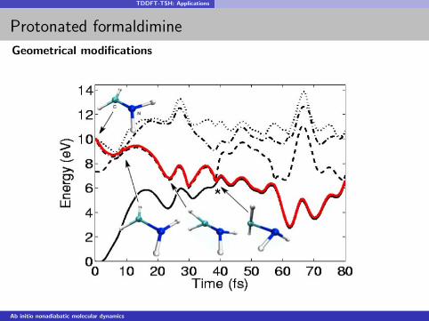
Protonated formaldimine
Geometrical modifications
Ab initio nonadiabatic molecular dynamics
TDDFT-TSH: Applications
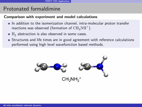
Protonated formaldimine
Comparison with experiment and model calculations
In addition to the isomerization channel, intra-molecular proton transferreactions was observed (formation of CH3NH+).
H2 abstraction is also observed in some cases.
Structures and life times are in good agreement with reference calculationsperformed using high level wavefunction based methods.
Ab initio nonadiabatic molecular dynamics
TDDFT-TSH: Applications Oxirane - Crossing between S1 and S0
Oxirane
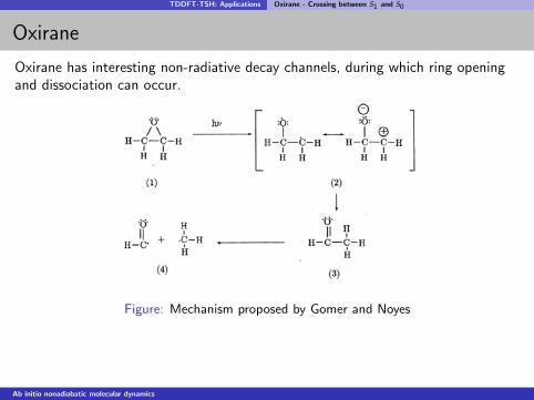
Oxirane has interesting non-radiative decay channels, during which ring openingand dissociation can occur.
Figure: Mechanism proposed by Gomer and Noyes
Ab initio nonadiabatic molecular dynamics
TDDFT-TSH: Applications Oxirane - Crossing between S1 and S0
Oxirane
Oxirane has interesting non-radiative decay channels, during which ring openingand dissociation can occur.Computational details
Isolated system
LR-TDDFT/PBE/TDA
SH-AIMD
30 trajectories (NVT) each of ∼100 fs.
JCP, 129, 124108 (2009).
Ab initio nonadiabatic molecular dynamics
TDDFT-TSH: Applications Oxirane - Crossing between S1 and S0
Oxirane
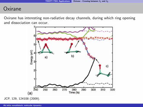
Oxirane has interesting non-radiative decay channels, during which ring openingand dissociation can occur.
JCP, 129, 124108 (2009).
Ab initio nonadiabatic molecular dynamics
TDDFT-TSH: Applications Oxirane - Crossing between S1 and S0
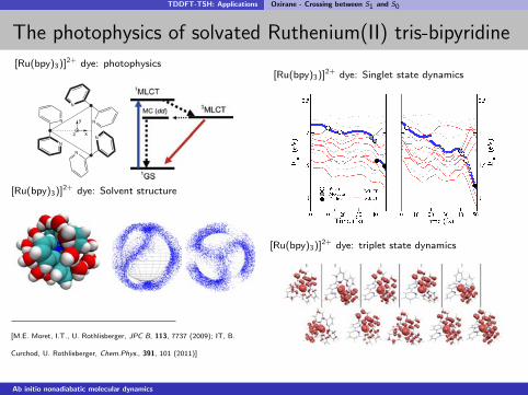
The photophysics of solvated Ruthenium(II) tris-bipyridine
[Ru(bpy)3)]2+ dye: photophysics
N
N
N
N
N
N
x
y
z
[Ru(bpy)3)]2+ dye: Solvent structure
[M.E. Moret, I.T., U. Rothlisberger, JPC B, 113, 7737 (2009); IT, B.
Curchod, U. Rothlisberger, Chem.Phys., 391, 101 (2011)]
[Ru(bpy)3)]2+ dye: Singlet state dynamics
[Ru(bpy)3)]2+ dye: triplet state dynamics
Ab initio nonadiabatic molecular dynamics
TSH with external time-dependent fields
1 Ab initio molecular dynamicsWhy Quantum Dynamics?
2 Mixed quantum-classical dynamicsEhrenfest dynamicsAdiabatic Born-Oppenheimer dynamicsNonadiabatic Bohmian dynamicsTrajectory Surface Hopping
3 TDDFT-based trajectory surface hoppingNonadiabatic couplings in TDDFT
4 TDDFT-TSH: ApplicationsPhotodissociation of OxiraneOxirane - Crossing between S1 and S0
5 TSH with external time-dependent fields
Ab initio nonadiabatic molecular dynamics
TSH with external time-dependent fields
TSH with external time-dependent fields
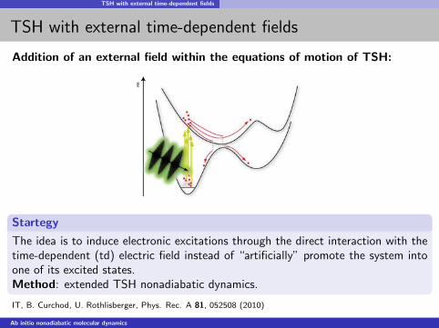
Addition of an external field within the equations of motion of TSH:
Startegy
The idea is to induce electronic excitations through the direct interaction with thetime-dependent (td) electric field instead of “artificially” promote the system intoone of its excited states.Method: extended TSH nonadiabatic dynamics.
IT, B. Curchod, U. Rothlisberger, Phys. Rec. A 81, 052508 (2010)
Ab initio nonadiabatic molecular dynamics
TSH with external time-dependent fields
TSH with external time-dependent fields
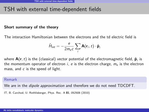
Short summary of the theory
The interaction Hamiltonian between the electrons and the td electric field is
Hint = − e
2mec
∑i
A(ri , t) · pi
where A(r, t) is the (classical) vector potential of the electromagnetic field, pi isthe momentum operator of electron i , e is the electron charge, me is the electronmass, and c is the speed of light.
Remark
We are in the dipole approximation and therefore we do not need TDCDFT.
IT, B. Curchod, U. Rothlisberger, Phys. Rec. A 81, 052508 (2010)
Ab initio nonadiabatic molecular dynamics
TSH with external time-dependent fields
External field within TSH
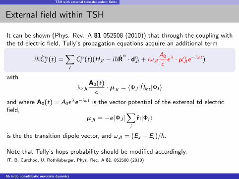
It can be shown (Phys. Rev. A 81 052508 (2010)) that through the coupling withthe td electric field, Tully’s propagation equations acquire an additional term
i~CαJ (t) =
∑I
CαI (t)(HJI − i~R
α · dαJI + iωJIA0
cελ · µαJI e−iωt)
with
iωJIA0(t)
c· µJI = 〈ΦJ |Hint |ΦI 〉
and where A0(t) = A0ελe−iωt is the vector potential of the external td electric
field,µJI = −e〈ΦJ |
∑i
ri |ΦI 〉
is the the transition dipole vector, and ωJI = (EJ − EI )/~.
Note that Tully’s hops probability should be modified accordingly.IT, B. Curchod, U. Rothlisberger, Phys. Rec. A 81, 052508 (2010)
Ab initio nonadiabatic molecular dynamics
TSH with external time-dependent fields
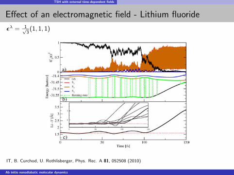
Effect of an electromagnetic field - Lithium fluoride
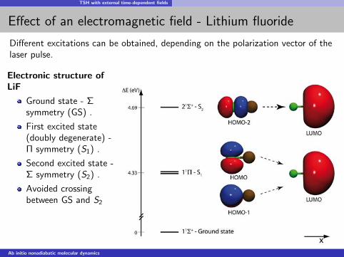
Different excitations can be obtained, depending on the polarization vector of thelaser pulse.
Electronic structure ofLiF
Ground state - Σsymmetry (GS) .
First excited state(doubly degenerate) -Π symmetry (S1) .
Second excited state -Σ symmetry (S2) .
Avoided crossingbetween GS and S2
Ab initio nonadiabatic molecular dynamics
TSH with external time-dependent fields
Effect of an electromagnetic field - Lithium fluoride
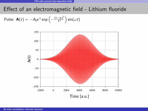
Pulse: A(t) = −A0ελ exp
(− (t−t0)2
T 2
)sin(ωt)
Ab initio nonadiabatic molecular dynamics
TSH with external time-dependent fields
Effect of an electromagnetic field - Lithium fluoride
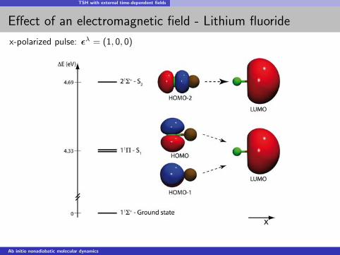
x-polarized pulse: ελ = (1, 0, 0)
Ab initio nonadiabatic molecular dynamics
TSH with external time-dependent fields
Effect of an electromagnetic field - Lithium fluoride
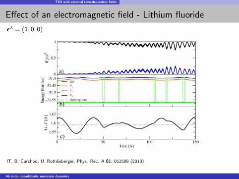
ελ = (1, 0, 0)
IT, B. Curchod, U. Rothlisberger, Phys. Rec. A 81, 052508 (2010)
Ab initio nonadiabatic molecular dynamics
TSH with external time-dependent fields
Effect of an electromagnetic field - Lithium fluoride
ελ = 1√3
(1, 1, 1)
IT, B. Curchod, U. Rothlisberger, Phys. Rec. A 81, 052508 (2010)
Ab initio nonadiabatic molecular dynamics
Recommended