't -fZ'
Vk - t) A .
** s- A' 4 ~ o A y r 'I,
I "'~~~ j4oI O
AA .3 *0 ~V AA
.... . .
7~ 7

DISCLAIMER NOTICE
THIS DOCUMENT IS BEST QUALITYPRACTICABLE. THE COPY FURNISHEDTO DTIC CONTAINED A SIGNIFICANTNUMBER OF PAGES WHICH DO NOT
..REPRODUCE LEGIBLY.
SIMPLIFIED FORN!S 01"PRELIMINARY TRAJECTORY (,At.(.: LA! ION
FOR GUN-V.'\I'NCHED . iI I ES
b
G.V, PARKN.,OIN
SRI-R-19
AUGUST 1967
SPACE RESEARCH INSTIfUTEOF McGILL UNIVERSITY892 Sherbrooke SL. W.Montreal 2, Quebec
Canada
d ?~(-
TABLE OF CONTENTS
lPa ge
1.0 INTRODUCTION I
2.0 FUNPAMENTAL ASSUMPTIONS .3
2.1 Basic Equation of Motion along Trajectory 3
.2 Acrodynamic Drag cf Gun-Launched Systems 5
2.3 The Model Atmosphere 10
3.0 GLIDE TRAJECTORIES 14
3.1 Evaluation of Drag Integral 14
3.2 Zero-Drag Glide Trajectories 17
3.3 Approximations for Glide Trajectories with Drag 18
3.4 Calculation Procedure for Constant-g Glide Trajectories 21
3.5 Discussion 28
4.0 ROCKET POWERED TRAJECTORIES 31
4.1 Evaluation of Elevation Angle 31
4.2 Evaluation of Drag Integral 3S
4.3 Determination of Velocity and Trajectory Parameters 40
4.4 Discussion 44
5.0 HIGH ALTHIUDE AND ORBITAL TRAJECTORIES
5.1 Effect of Earth Rotation 5
5.2 Fundamental Equations and Solutions 47
REFERENCES

- iii-I
Page
Appendix A: Traiectory Equations for Zero Drag, Zero Thrust A-1
Constant g
Appendiv B: Caiculations for Martlet 2A Shots B-1
Appenoix C: Calculations for Projectile Trajectory C-i
Appendix P: TraiecLory Equations for Vehicle under Rocket D-I
Thrust, with Zero Drag, Constant g
Appendix E: MarLlet 4 Trajectory Calculations E-1
r
t
EI

- iv-
LIST OF FIGURES
Page
I. Vehicle Trajectory Parameters 4
2. Analytical Approximation to Drag Coefficient 8
3. Atmospheric Pressure vs Altitude 13
4. Atmospheric Sound Speed vs Altitude 13
5. Total Drag Decrement Integral 16
6. Basis of Horizontal Range Increment Approximation 20
7. Universal Zero-Drag Constant-g Trajectory 22
8, Martlet 2A Shot IOWA Trajectory 24
9. Velocity vs Altitudf for Mattlet 2A Shot 25
10. Altitude vs Elapsed Time for Martler 2A Shot 26
11. Martlet 2A Trajectories 27
12. Trajectory Comparisons for Projectile 29
13. Sin 0 vs Ck forAT = 0.25 34n n
14. Altitude-Mass Relation for Zero-Drag, Constant-Thrust Motor 37
[5. -) vs h for Cape Kennedy Standard Atmosphere 39a
16. Vehicle Velocity Diagram 48
17. Trajectory Variables 19
18. Spherical Geometr for Range 53
LIST OF TABLES
1. Drag Decrement Integrals Al and I 15
2. Martlet 4 Trajectory Calculations for HARP Case 3046 43

V
NOMENCLATURE
m vehicle mass, slugs
2g acceleration of gravity, ft/sec
h vehicle vertical altitude, ft
X vehicle horizontal range, ft
0 vehicle trajectory elevation angle from horizontal
t time, secs
V vehicle velocity, relative to earth, fps
V. rocket motor exhaust velocity, fpsJ
b dm rocket motor burning rate, slugs/secdt
D = CD . A aerodynamic drag on vehicle, lbs
dmF -V d- rocket motor thrust on vehicle, lbs
j dt
A vehicle cross-section reference area, sq ft
CD drag coefficient
q P 2 dynamic pressure, psf2
ratio of atmospheric specific heats at constantpressure and constant volt:me
V= vehicle Mach number
a
p L RT atmospheric pressure, psf
a atmospheric sound speed, fps
T atmospheric temperature, RankineR atmospheric gas constant, ft2 /sec 2 oRankine
atmospheric density, slugs/ft3
~VdNR Vd vehicle Reynolds number
d ve' icle base diameter, ft
2Y atmospheric kinematic viscosity, ft /sec
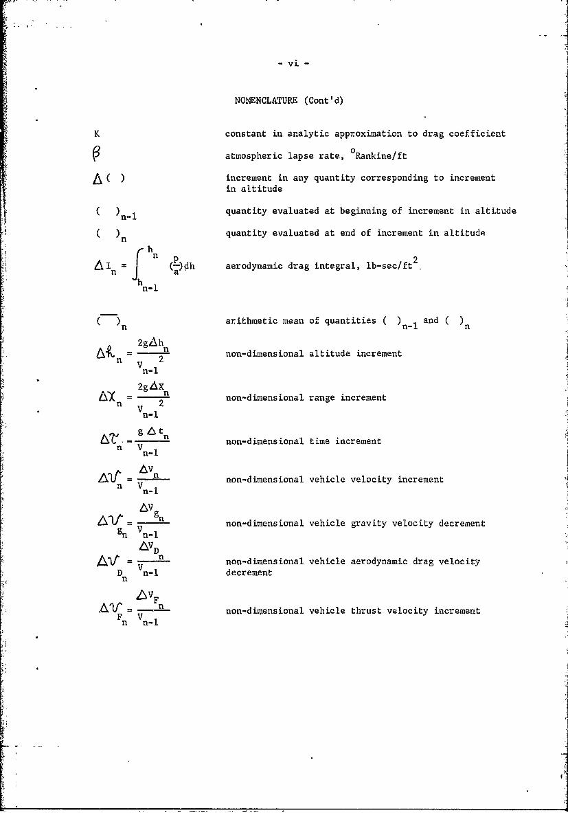
- vi -
NOMIENCLATURE (Cont' d)
K constant in analytic approximation to drag coefficient
0v atmospheric lapse rate, Rankine/ft
( increment in any quantity corresponding to incrementin altitude
( )n-1 quantity evaluated at beginning of increment in altitude
( )n quantity evaluated at end of increment in altitude
hnI
A~ =(P)dh aerodynamic drag integral, ib-sec/ft2
( )n arithmetic mean of quantities n-i and n
2gihn V non-dimensional altitude increment
Sn- 1
2gAXn g2 non-dimensional range increment
Vn. I
g t.= n non-dimensional time incrementn V n. 1
n= non-dimensional vehicle velocity incrementn-i
g n non-dimensional vehicle gravity velocity decrement
g Vn~gn Vn-I
AVD
V n non-dimensional vehicle aerodynamic drag velocityD n- decrementn
vF
AV = n non-dimensional vehicle thrust velocity incrementFn Vn. 1
n n-
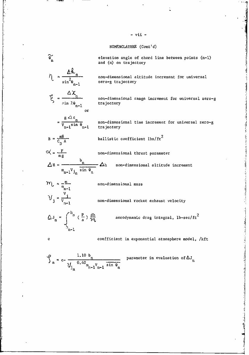
-vii-
NOMENCLATURE (Cont:d)
[ n elevation angle of chord line between points (n-i)and (n) on trajectory
n
2 non-dimensional altitude increment for universalsin 9 n-1 zero-g trajectory
= n non-dimensional range increment for universal zero-g
-in 29n trajectoryn-Ior
g 4\ tn
V sin 9 non-dimensional time increment for universal zero-gn-Is n-1 trajectory
B = mg ballistic coefficient ibs/ft 2
D A
= F non-dimensional thrust parametermg
bA H n h non-dimensional altitude increment
m Vn sin nn-I n n
Y = mnon-dimensional massn- IV.
j Vn. non-dimensional rocket exhaust velocity
f hn P d
AJ = (f - dh aerodynamic drag integral, lb-sec/ft2
n a ,,I
n-I
c coefficient in exponential atmosphere model, /kft
1.10 bi. 0 m n parameter in evaluation of 6J
n _ 0.40 sin
nn mn-1in-l n
i
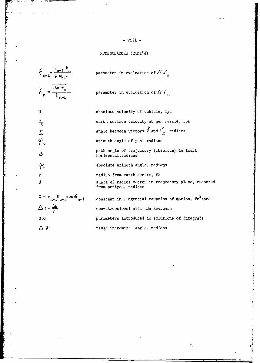
F - viii-
NOMENCLATURE (Cont' d)
V nIb
n- l g n parameter in evaluation of LV
&n = sin n parameter in evaluation of L/n
U absolute velocity of vehicle, fps
UE earth surface velocity at gun muzzle, fps
angle between vectors V and bE, radians
Kv azimuth angle of gun, radians
path angle of trajectory (absolute) to local.& horizontal,radians
absolute azimuth angle, radians
r radius from earth centre, ft
0 angle of radius vector in trajectory plane, measuredfrom perigee, radians
n-i n-iC n-1 constant in . ngential equation of motion, ft 2/sec
LL --- non-dimensional altitude increase
S,Q parameters introduced in solutions of integrals
0 0' range increment angle, radians
1.0 INTRODUCTION
The precise calculation of the motion of a gun.-launcha. vehicle
through and out cf the atmosphere depends on a large number of parameters.
These include the environmental parameters of atmospheric properties and
gravity, which vary with altitude, and effects of the earth's rotation,
which depend also on the launch direction. Then there are the -vehicle
parameters of mass, external size and shape, raotion of control surfaces,
specific impulse, mass ratio, and ignition and burning time of any rocket
motors, and auxiliary or directional thrust systems. Finally there are
the gun launch parameters of initial velocity and direction.
Inclusion of the accurate variation of these pareters alro g the
trajectory leads to equations of motion which cannot be solved exactly,
Consequently, various numerical couputer programs have been devised, and
these satisfactorily determine trajectories for given vwlues of the para-
meters. In general they also can rapidly display the resul:s of arbitrary
variation of the parameters, so that optimum t ajectories among those
calculated can be selected.
This approach to trajectory calculation. while probablv essential
for accurate final calculations for a particular vehicle rrissior, suffers
from two serious defe.ts when applied to preliminary trajector, calculations,
in which possible missions for existing or proposed 7ehicles are !-ing con-
sidered. First, a computer may not ' e a! readily available as tbe require-
ments for a set of rapid preliminary calculations would indizate. Second,
and more serious, as in all numerical programs the output of numbers has to
be interpreted and analysed for trends ivt the light of the parameter input.
There are no analytical forms linking input and output, from which trends
could be discerned and predictions made, and as a result it is difficult
to reach clearcut decisions about new vehicle missions.
It would therefore be useful if simplified forms of the governing
equations could be developed which would retain the essential features of
the exact equations and produce vehicle trajectories and other performance
characteristics accurate to within 5 or even 10 percent, while providing
straightfcrward analytical or graphical links between the various parameters
and the resulting performance. That is the main purpose of the present
report. An additional purpose is to provide, for reference, derivations
of some of the important equations governing the motion of gun-launched
vehicles.
-3-
2.0 FUNDAMENTAL ASSUMFTIONS
It will be assumed that the vehicles considered are aerodynamically
symmetric wi.th respect to their trajectory at all times, so that they
experi(-nce no lift, merely drag, in their motion through the atmosphere.
Any rocket thrust will be assumed to be constant in magnitude, and directed
back aloag the trajectory, so that the vehicles are turned only by gravity.
During motion of the vehicle either through the atmosphere or under the
action of rocket thrust, or both, it will be assumed that the gravitational
force is constant in magnitude and direction. The above assumptions will
be accurate to within 3 percent for almost all cases.
2.1 BASIC EQUATION OF MOTION ALONG TRAJECTORY
In the light of the above assumptions, Figure I serves to define
the equation of vehicle motion alonS its trajectory. Newton's Second Law
of Motion requires 'Resultant External Force along Trajectory = Time Rate
of Change of System Momentum along Trajectory'. The external forces are
the tangential component of gravitational force mg sin 9 and the aerodynamic
drag D. The rocket motor thrust F is an internal force accouted for by
the system momentum change. Consider the vehicle at time t when its mass
is m and its velocity V. After an infinitesimal time increment At the
rocket exhaust of constant velocity V has expelled mass - Am (the minus
sign preserves the algebraic sign convention) and the velocity of the
vehicle has increased to V + AV. Thus Newton's Second Law becomes:
SM
Figure 1 Vehicle Trajectory Parameters
-7-
-- 5 "
-D- g i(mi m+ M) (V + 6V) A~M(V V1f Vt-d
dV d imdj dt
or F -D -mg s in 9 m dtV (2.1)
dm
dh-=V=snV9 2.2
ddt
r~ ish h
m m
nn
h - - s n s in dh2gn -I j m J mVsnIdh-g
h n(2.3)
or~Vn 'rJF V D -64
n n gn
In Eq. (2.3), the integrals for the velocity decrements from aerodynamic drag
and gravity cannot be evaluated by quadratures without the introducticn of
further assumptions. The integral for &V D is considered first.n
2.2 AERODYNAMIC DRAG OF GUN-LAUNCHED SYSTEMS
Aerodynamic drag is conventionally expressed in terms of a drag
coefficient CD through the defining equation
D = CD q A (2.4)
where A = reference area = projected frontal area of body for a rocket or
S6
gun-launched vehicle,
q = dynamic pressure.
In high speed aerodynamics the drag is caused by both the compres-
sibility and friction of the air, and therefore the drag coefficient depends
upon both Mach number M and Reynolds number NR,
CD = CD (M, NR) (2.5)
where M= = Vehicle Mach numbera
NR= V d = Vehicle Reynolds number
a = local atmospheric speed of sound
d = vehicle base diameter
= local atmospheric kinematic viscosity.
It is convenient to express the dynamic pressure in terms of Mach number,
q =.2M2 (2.6)2
where ' = ratio of atmospheric specific heats at constant pressure at d
constant volume
= 1.40, assumed constant
p - local atmospheric pressure.
The dependence of C on M and N is complex, even for simple vehicleD R
shapes, and it has been common to make approximations in perfoimance analysis.
In the present analysis, the nature of gun-launching permits a very simple
and useful approximation to be made. All gun-launched vehicles have initial
:1-j

-7-
Mach numbers greater than 3, and even without rocket boost, vehicle Mach
numbers will rarely fall much below 3 during motion through atmosphere
dense enough to produce significant drag. Therefore it is not necessary
to consider the drag variation of the vehicles in subsonic and transonic
flight (as is required for conventional rocket-launched systems). Only
the drag variation in supersonic and hypersonic motion need be considered
and this is much simpler.
Over the range of velocities through the atmosphere experienced
by a vehicle on a typical gun-launched mission, the variation of CD with
N will be quite small, and it is assumed henceforth thatR
0D = CD (M) (2.7)
only for a particular vehicle. This variation can be approximated quite
accurately in the supersonic and hypersonic range by the relation
C K (2.8)D M
where K is a constant chosen to provide the best fit of Eq. (2.8) to the
available data for the vehicle over the Mach number range of interest. In
Figure 2 such a fit is shown for the Martlet 2A glide vehicle, the data
being obtained from Reference I. In the figure the maximum deviation of
the approximate from the actual curve is 7.7 percent, and since it is clear
that positive and negative deviations will tend to cancel in the drag
integral of Eq. (2.3), and that in any case the actual values of CD may not
be accurately known at the time of the preliminary calculations for which
t'is analysis is intended, the approximation of CD by Eq. (2.8) is seen to
be satisfactory,

$ -8-
'. I,: OZ0
o
61
o Ii
4
lie
MAW_,_-II
fi
-9-
Therefore, Eq. (2.4) becomes
D - KYA p M (2.9)2
and the drag integral can be written
AV IK KA dh (fhn0Dn h sin (
n-1.
In the integrand in Eq. (2.10), (p/a) is a property of the local atmosphere,
and is a function of h only for a given model of the atmosphere. As the
vehicle climbs through the atmosphere after gun launch, sin 0 is a slowly
decreasing function of h which of course is unknown until the trajectory
is determined. However, the initial value is known, and because of the slow
decrease with increasing h, a sufficiently accurate average value sin G6
can be determined fr.om the equivalent zero-drag trajectory between the same
altitude limits. The drag integral can then be written
= KYA , dh2 sin 9 n J )(.1hn
For vehicles without rocket motors, or for glide sections of any
gun-launched vehicle trajectory, m is constant and Eq. (2.11) can be evalu-
ated directly. During motion through the atmosphere under rocket thrust,
m decreases at a constant time rate, and again the equivalent zero-drag
trajectory can be used to approximate m as an integrable function of h
between the same altitude limits.
The significant observation to be made from Eq. (2.11) is that,
I
-10-
within the accuracy of Eq. (2.8), the decrement in velocity experienced by a
supersonic or hypersonic gun-launcheG vehicle due to atmospheric drag is not
increased by increasing the launch velocity of tht vehicle, as one might
expect intuitively.
On the contrary, for a vehicle without rocket motor, or during a glide
section of any vehicle trajectory, the drag velocity decrement is nearly
independent of the vehicle velocity, which enters ouly through its rather
small effect on the value of sin 9n in Eq. (2.11), and here the effect of
i.ncreased launch velocity is to increase sin 9n and thus reduce the drag
decrement.
For a rocket-powered section of vehicle trajectory wit-h a motor of
given burning rate, the effect of increased launch velocity is to reduce
the decrease of vehicle mass m in passing through a given altitude increment,
and thus again reduce the drag velocity decrement.
In general, then, Eq. (2.11) shows that for any gun-launched vehicle,
the higher the launch velocity, the lower will be the resultig decrement in
velocity due to aerodynamic drag.
2.3 THE MODEL ATMOSPHERE
Before Eq. (2.11) can be integrated, the dependence of (p/a) on h for
the atmosphere under consideration must be put in suitable analytic f,:rm.
Here the model used assumes a linear variation of temperature T with altitude,
'I
<
1I
- !i -
T= Tn - (h - hnI) (2.12)
where
lapse rate = constant.
The air is assumed to obey the equation of state of a perfect gas
p = 0 RT (2.13)
where D = air density
R = specific gas constant
= 76f 2 2 oI= 1716 ft2/(sec2 . °Ra.nkine)'l
The additional relation needed is the vertical equilibritm equation for
the static atmosphere
dp_=dh " g (2.14)
If 0 and T are eliminated from Eqs, (2.12), (2.13), and (2.14) the
result is
dh R T, -@(h hnlj
ord =pgdD _ - dh
n Tri - (h hn 1 )jPn-i hn-1)
This equation is integrated directly to producE. the pressure-altitude
relation
CT, '(h~h) 6R2- Lj(2.15)Pn-1i no

- 12 -
The speed of sound in a perfect gas is given by
a = - (2.16)
and so, using Eq. (2.12),
a '- 1- - (h -Ii)(2.17)
Therefore, the required function for (p/a) is, with a little rearrangement
a Pnl )fTln1n
a 1~ T. -(h h OR1 (2.18)
For a particular atmosphere, is chcsen t fit the actual temperature
variation within given altitude limits. In this report, the reference
atmosphere is the Cape Kennedy Standard Atmosphere from Reference 2, and
a very good fit is obtained using 3 values of , as follows:
< h < 50.8 kft 3. 5 4oR/kft
oR50.8 <h /162.4 kft -2 = 1.235 /kft
162.4 <h < 270.6 kft @3= l.5740R/kft
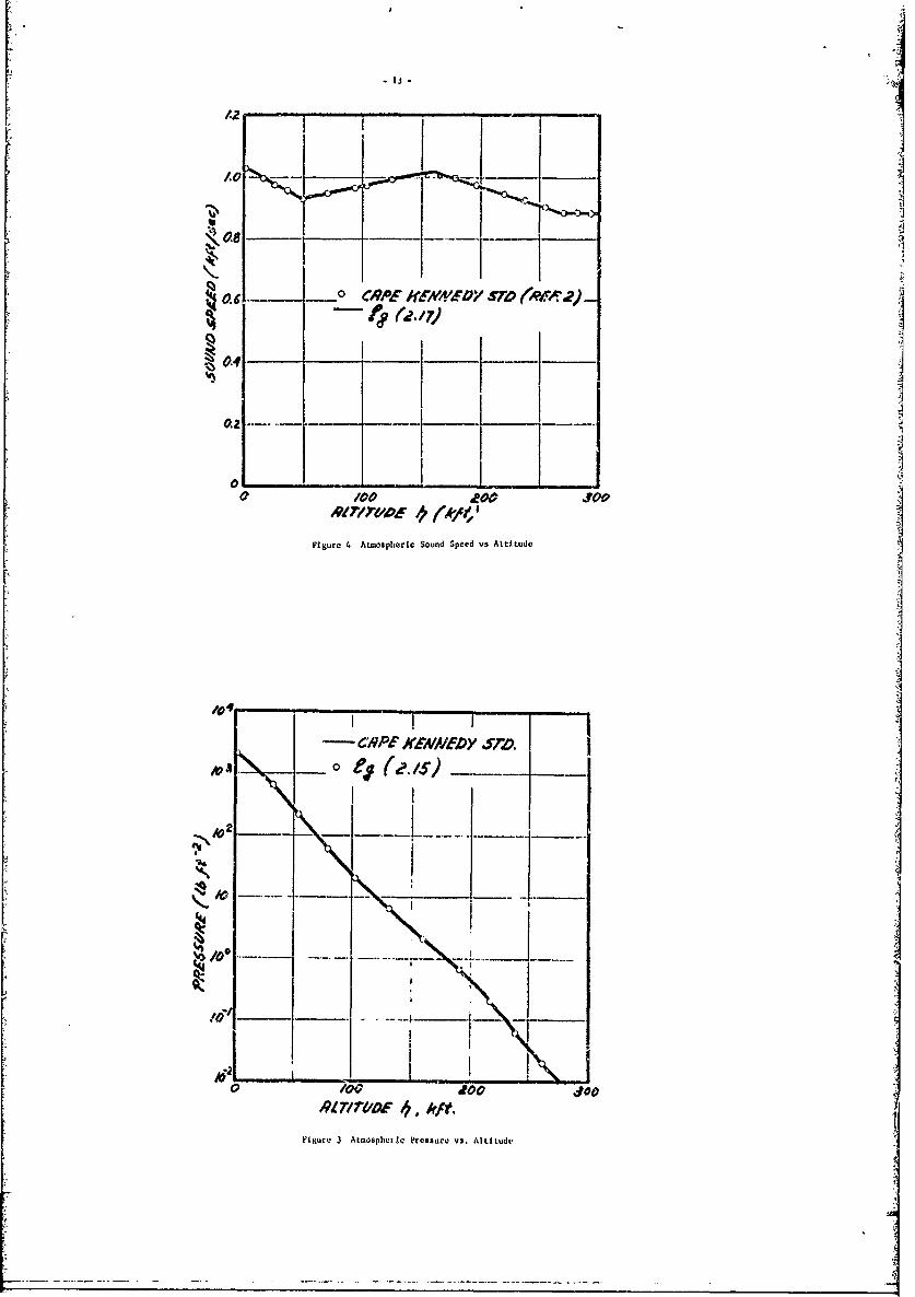
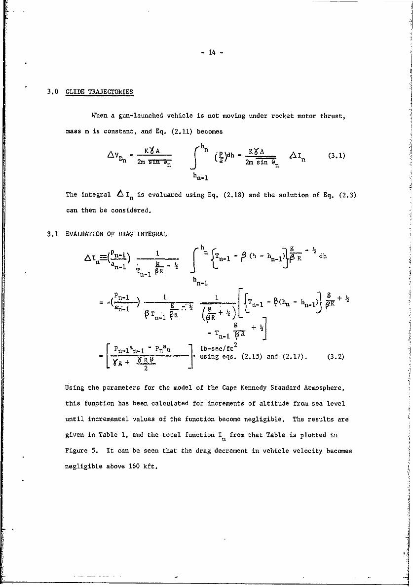
Figures 3 and 4 show the close agreement between the pressure and sound
speed from Reference 2 and the values given by Eqs. (2.15) and (2.17),
using the above values of ' . For this atmosphere, at sea level (h = 0):
Po 2125 psf, ao = 1138 fps, g = 32.15 ft/sec2
ft/sec"
1.2
-- ~ m 0v.c aQP if~y sTro (IA 2.~)0.4
0.2 ____I
0 /0 ~eo/ 3Z0
Figure 4 Armospheric Sound Speed vs Altitude
- I ' I "
,I I
oa - ; 7iZ7I.__44r/uE ,k,
Ftgue 3Atmsphe~e resure s. ~tludI
-14-
3.0 GLIDE TRAJECTOkMES
When a gun-launched vehicle is not moving under rocket motor thrust,
mass m is constant, and Eq. (2.11) becomes
AV KA rhn ( KYA AI (3.1)
AV~nnDn 2m stf 9Pd 2m sin 9n
n n~)h
hni1
The integral A In is evaluated using Eq. (2.18) and the solution of Eq. (2.3)
can then be considered.
3.1 EVALUATION OF DRAG INTEGRAL
aPn.lI I z h gRn-n
hn-I
T +
- T1 R' R
rpn'lan 'l " Pnan 1 lb-sec/ ft2
[ 'g + R_ ,using eqs. (2.15) and (2.1.7). (3.2)2
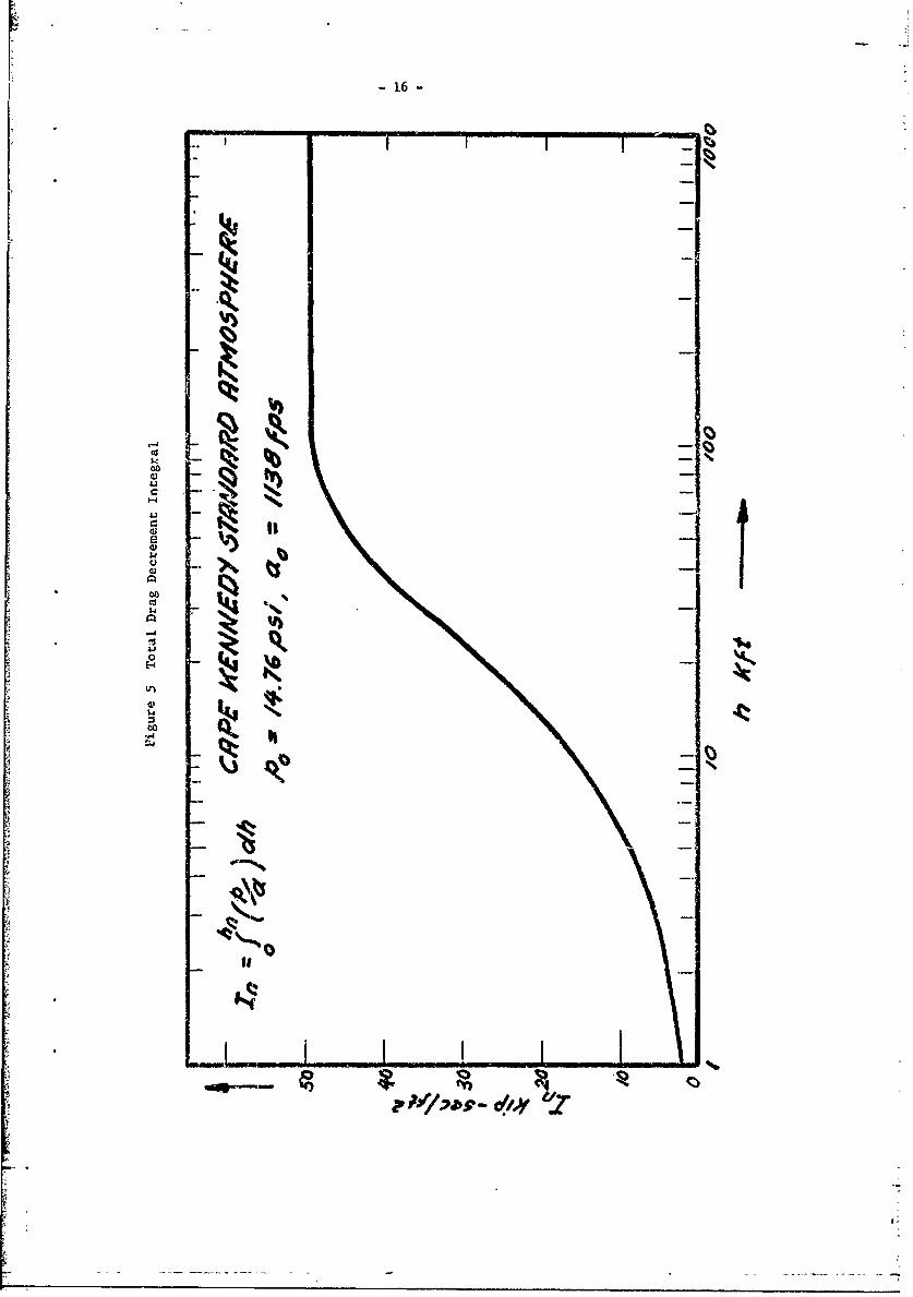
Using the parameters for the model of the Cape Kennedy Standard Atmosphere,
this function has been calculated for increments of altitude from sea level
until incremental values of the function become negligible. The results are
given in Table 1, and the total function I from that Table is plotted il' n
Figure 5. It can be seen that the drag decrement in vehicle velocity becomes
negligible above 160 kft.
L~

-15-
TABLE I
Drag Decrement Integrals ~In and I n
No. h 1 2 In No. h I V. 2 inkft lbasec/ft2 lb-sec/ft2 kft lb-sec/ft lb-sec/ft2
0 0 0 0 14 65.6 2740 47100
1 1.00 2080 2080 15 82.0 1370 48500
2 2.00 1950 4030 16 98.4 630 49100
3 3.28 1810 5840 17 114.8 288 49400
4 6.56 5420 11260 18 131.2 141 49500
5 9.84 4660 15920 19 147.6 67 49600
6 13.12 4240 20160 20 162.4 34 49700
7 16.40 3760 23920 21 180.5 22
8 19.68 3200 27120 22 196.8 11
9 26,24 5420 32540 23 213.2 6
10 32.80 4650 37190 24 229.6 3
11 39.36 3300 40490 25 246.0 1
12 45.92 2520 43010 26 262.4 1
13 50.84 1390 44400 27 270.6 0
TOTAL 49,700 lb-sec/ft2
[
-A
- 16 -
.4'
k, -
1-4
U II
Ln3
IlI,
w
o
I' $4
Q 4 ,
Ai
7'
I ~ '~4~9 -

- 17 -
3.2 ZERO-DRAG GLIDE TRAJECTORIES
The equations of motion for a vehicle moving without rocket thrust
or atmospheric drag under constant g are very simple. They are useful
in the present analysis both in providing a basis for approximating certain
functions in Eq. (2.3), and in themselves as giving sufficiently accurate
results for the upper parts of vehicle trajectories high enough to neglect
aerodynamic drag but not so high as to require the inclusion of g variations.
The first relation needed is obtained directly from the conservation
of mechanical potential and kinetic energy:
h-hVn21 - Vn2 (33)n n-l 2g
The other relations needed are obtained by manipulating the equations of
vehiclc motion in the X- and h- directions (see Figure 1), and are derived
in Appendix A:
6 tan n AX sec 2 2nl n (3.4)
n sip2 0n-l n n- n
sinsin! I, 1 - . (3.5)
orCos 9n- 1
Cos9 0 _ . (3.6)
where
= V (h n h = 2 (X X I ) (3.7)V2 n 1-_ v n nn-i
.--
18
3.3 APPROXIMATIONS FOR GLIDE TRAJECTORIES WITH DRAG
For a vehicle moving without rocket thrust, Eq. (2.3) can be
written, using Eq. (3.1):
n Dn gn
K ? A Al -g dh (3.8)2m F n V
nhn-i
If there were no aerodynamic drag, Eq. (3.3) could be used, and written
in the form showing the velocity decrement caused by gravity:
2g (hn - hl)v -Vf- V L
n n-IVn n- = n + Vn- 1
or AV - g Ah V (3.9)n " gn
Vn
where
V= (V + V) + AV (3.10)n n-l n n-I n
It is now assumed that AVgn in Eq. (3.8) can be approximated by an expres-
sion of the form of Eq. (3.9), with V the arithmetic mean of the actual
V and V:n-i n'
nv~ VD nnor, multiplying through by V and using Eq. (3.10):
2-V n + (Vn + VD) Vn + (VnlLxVD +gLh)=0.
n n) n

19
Solving for / V n, and dividing through by Vnl
v VD VDnnn ) + + n ) 2 V n
Vn-1 n In-1 n-1
or A n = - (1 + A- n) + (I - ) ._n (3.11)
n n&v &VD
where , -~~ -a (3.12)where L_ r n =V n A-l = Vn1312
n-I n n-i
Before Eq. (3.11) car be used to calculate velocity decrements along a
glide trajectory, a method of determining sin 9 in the expression forn
LV D must be given. It can be shown thatn h
1 dh
sin 9
hn-i
is a good approximation to
j n dhsin9
hn-1
where sin 9 = (sin 9n- + sin 9 n) (3.13)
and sin 9 is given by Eq. (3.5).n
For example, with sin 9nl = 0.50 and sin 9 = 0.25, the approximate formula
is only 1% higher than the exact integral.
- 20-
Therefore sin 9 as defined by Eq. (3.13) is used in Eq. (3.1).
In the calculation procedure next to be described, the fundamental inde-
pendent variable is the altitude increment A h . Calculation of then
vehicle trajectory requires corresponding values of the horizontal
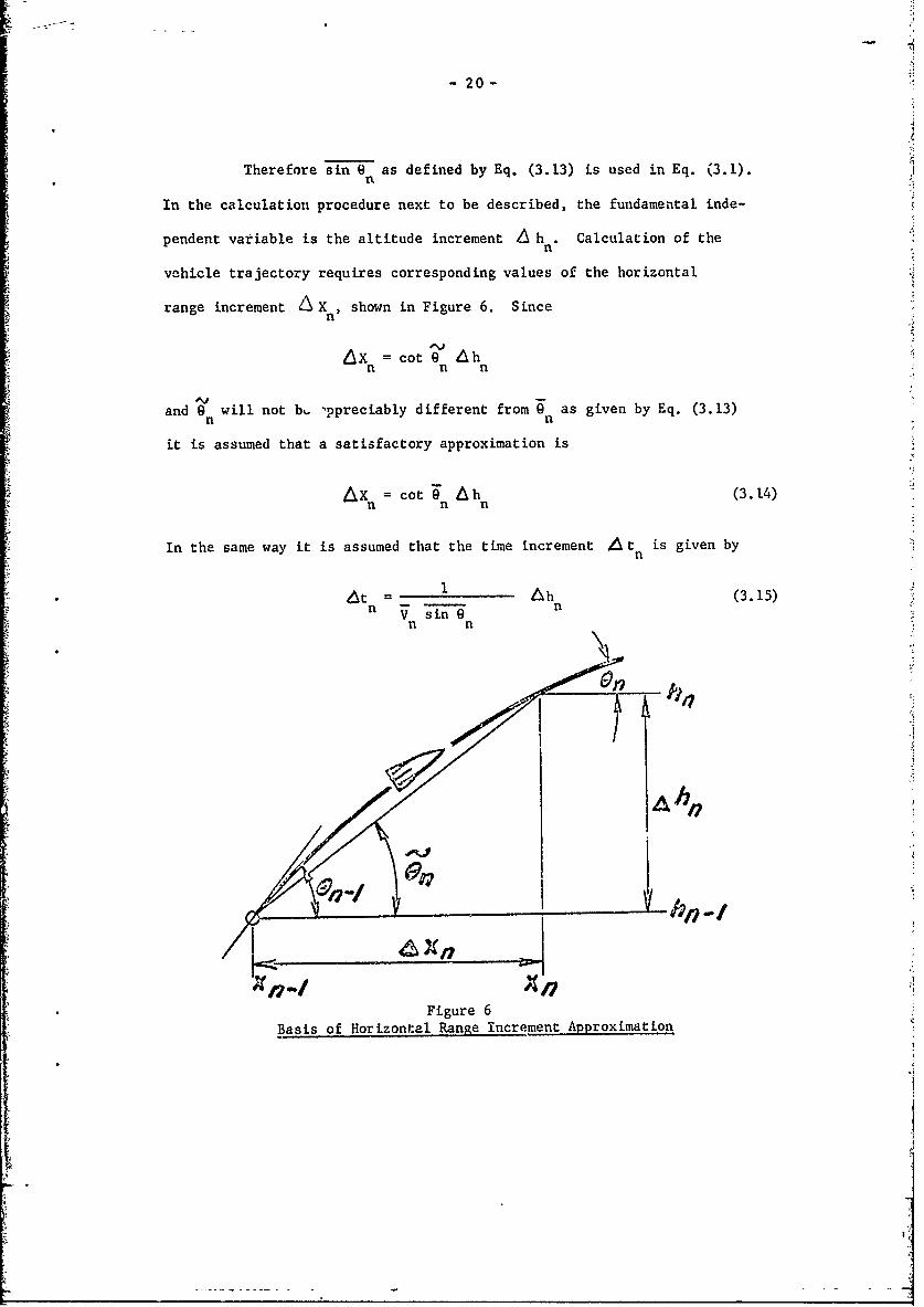
range increment A Xn, shown in Figure 6. Since
6 = cot 9 hn n n
and 9 will not b%. ppreciably different from 9 as given by Eq. (3.13)n n
it is assumed that a satisfactory approximation is
a = cot 9n hn (3.14)
In the same way it is assumed that the time increment L t is given byn
* = (3.15)n V sin 9
n n
n XI,
G7
Figure 6Basis of Horizontal Range Increment Approximation
io-
-21-
3.4 CALCULATION PROCEDURE FOR CONSTANT-g GLIDE TRAJECTORIES
For a given vehicle launched under given conditions in a given
model atmosphere, the following parameters are known:
g, m, A, K, , Vo,
K6A
The factor 2- in 6V can therefore be calculated. The drag integral I2m D n
ncan be determined for each altitude increment &h from Figure 5 or Table
n
1. The altitude to which the aerodynamic drag is significant is broken
down into a few increments, the number increasing with the accuracy desired.
Thus four increments should be sufficient for most preliminary calculations.
while one may be enough for a rough calculation.
The procedure is then to use the equations of 3.2 and 3.3 to
determine the velocity decrentent, horizontal range increment, time increment,
and final elevation angle for each altitude increment. Above the final
atmospheric altitude increment, the equations of 3.2 and Appendix A
are used to calculate the remainder of the trajectory to its apogee.
Alternatively, Eq. (3.4) for the parabolic zero-drag trajectory can be put
in the universal form:
24 (3.16)
where and are defined in Appendix A. Eq. (3.16) is plotted in
Figure 7 and all zero-drag, constant-g glide trajectories can be determined
from it.
... .... .... ... .... ...

[,22- -,
I-I
14 2
'7i
.4 ,, ,, , '1 a. i oo.(n 6 ,ai)ena
.,?. . . .8 Si.0 r
Figure 7 Universal Zero-Drag Constant-g Trajectory
'I

- 23 -
In greater detail, the procedure for the atmospheric part of the
trajectory, given hn, A hn, Vn 9n-l' is to calculate nfrom
Eq. (3.7) and use this to calculate sin 9 from Eq. (3.5) or cosn fromn n
Eq. (3.6). (The latter is more convenient for values of 9 near 90o.)n-I
This determines the new elevation angle 9 . Next sin 9 is found fromn n
Eq. (3.13), giving 9 . With Ai determined for the given A b fromn n n
Figure 5 or Table 1, #V is calculated from Eq. (3.8), and A-Lr fromD Dn nEq. (3.12). Now Aiu can be calculated from Eq. (3.11), and this gives the
n
velocity change AV from Eq. (3.12). The range increment &X is calculatedn n
from Eq. (3.14) and this gives the new X corresponding to h . The timen n
increment At is calculated from Eq. (3.15), giving the new t . The newn n
velocity Vn is given by adding AVn to V n-. The procedure is then
repeated for the next altitude increment.
Figure 8 gives the application of the procedure to the trajectory
of the Martlet 2A, IOWA shot from the Barbados 16" gun on March 'j, 1965.
Results of calculations with both four and one atmospheric altitude increments
are compared with radar-determined trajectories of the actual shot from
Reference 1, and with the standard HARP trajectory from Reference 3. Curves
are given for vehicle weights of both 170 lbs and 180 ibs, since tOe actual
vehicle weighed 170 ibs, while the HARP trajectory was calculated for 180 lbs.
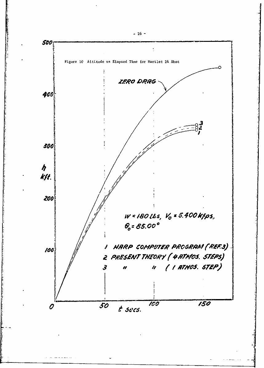
Figures 9 and 10 show the variation of vehicle velocity and elapsed time with
altitude, up to the apogee, for the 180 lb vehicle as calculated by the present
method with both four and one atmospheric steps, and by the standard HARP
computer program. Calculations for Figures 8, 9 and 10 are tabulated in
Appendix B. In Figure 11, the 180 lb trajectories a, e compared again for
greater clarity.

24-
'44
AMRf Af_
RAP rR5W7 is
-IR PR01O F8 A
'---0Pe5-l MORY f~rS7,6
/1 i4 /8 IAF Ir~ 7
0 .QOR rR0*Js9c0 W -. /0 l
0 /604lb0
Figur 8S f /70le 2ASolIWbsaetr

-25-
00
'41'
-44
414
-,4
'a0
-~26
Figure 10 Altitude vs Elapsed Time for Martlet 2A Shot
400
I3
1010
z? PA3.eSeiVT TwoA'y (##h'TA 1O fzeops)
$ '~ (/ #rev. $rep)

-27-
44E
AV- pei- z S W AWRY (4 vrTyos. SrfP5)
Figure 11 Martlet 2A Trajectories
28
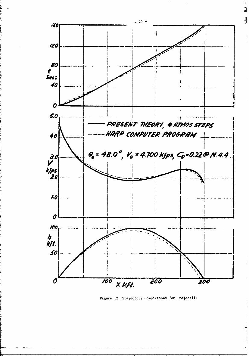
A comparison that makes greater demands on the method is shown in
Figure 12. Here a projectile is analyzed from launch to impact, with the
entire trajectory low enough that measurable aerodynamic drag is experienced
throughout. The present method with four atmospheric altitude increments
for both climb to and descent from 80,000 ft and altitudes above 80,G00 ft
assumed non-atmospheric, is compared with the standard HARP computer program,
and elapsed time, velocity, and altitude are plotted against range. Cal-
culations are given in Appendix C.
3.5 DISCUSSION
The calculation procedure is very simple and, even for a choice
of several altitude increments in the atmosphere, it can be carried out
quickly using just a slide rule or a slide rule and trigonometric tables.
Despite this simplicity, the curves of Figures 8, 9, 10, 11 and 12 show
that it produces accurate results, agreeing closely both with actual
measurements and with more exact numerical procedures.
Figure 8 shows that a four-step atmospheric calculation Dredicts
the observed trajectory of Martlet 2A IOWA very closely, with the apogee
only 1.8% higher than that observed.
Figures 9, 10 and 11 show that the four-step atmospheric cal-
culation for a 180 lb Martlet 2A gives results nearly identical with those
of the HARP computer program. Moreover, even the one-step atmospheric cal-
culation gives good accuracy in this example, the velocity values and
elapsed times lying quite close to the HARP curves, and the trajectory
having an apogee only 3.0% high.
'7
____ __ _ ____ ____ __ 29-
00-.0
AV - ----
k 5 -I _ _
x .----
Fiur 12 Taetr Coprsn fo Pojc i

-30-
Figure 12 shows that even a low-altitude prcjectile trajectory is
calculated from launch to impact with good accuracy by the method. Errors
in calculated quantities at points along the trajectory are generally less
than 5%, and in some of the more important quantities the errors are:
range (+1.9%), apogee (+4.2%), range at apogee (+1.1%), velocity at apogee
(-3.5%), time to impact (+4.1%), time to apogee (+3.3%), velocity at impact
(-9.0%). The larger error in impact velocity is caused by matching the
formula for drag coefficient, CD = K ,to the curve used in the computer
program at M = 4.4. This gives excellent agreement at the higher Mach
numbers, but produces higher drag at the lower Mach numbers preceding impact.
i1
I
i
---

- 31 -
4.0 ROCKET POWERED TRAJECTORIES
The altitude change during the burning of a rocket motor stage of
a vehicle is in general small enough to permit neglect of the change in g
during motor burning. For altitudes below about 160 kft, however, effects
of aerodynamic drag cannot be neglected, and the vehicle velocity increment
AV resulting from rocket thrust is then given by Eq. (2.3), with the dragn
velocity decrement /n VD given by Eq. (2.11) and the gravity velocityn
decrement tAV given by Eqs. (3.9) and (3.10). In this section thegn
evaluation of &V from Eq. (2.3) and the determination of other rocket-n
powered trajectory parameters are described.
4.1 EVALUATION OF ELEVATION ANGLE
Before &V D can be evaluated from Eq. (2.11), a suitablen
determination of the mean value sin 0 must be made for a rocket-poweredn
trajectory, and the dependence of mass m on altitude h during thrusting
must be expressed so that the integral can be evaluated.
As in the glide trajectories of the previous section, the deter-
mination of sin 0 is approached by neglecting the direct effect of drav-n
on elevation angle. It is shown in Appendix D that in zero-drag, 'castant-g
conditions, the differential equation governing the variatun of elevation
angle 9 with time t under the action of thrust F is
22+ (2 tan 9 -C Qsec 9)(~ 0(4)
dt
where
[ TF=fg

- 32 -
For the constant thrust rocket motors under consideration here, OC varies
with time and Eq. (4.1) is a fairly complicated nonlinear differential
equation. Two special cases of the equation can, however, be treated
easily. If O .= 0, of course, Eq. (4.1) governs zero-drag glide trajectories
and the solution of Eqs. (3.5) and (3.6) is obtained. If OC = constant, it
is shown in Appendix D that Eq. (4.1) is easily reduced to the integral form:
9n c-2 cos D
cos 0 d 9 n-l n=O -sn ) (4.2)(1 + sin 0) (1 + sin 9n l)
@n-1l
n- 1gAX
where e - nn Vn1
This is integrable by quadratures for cC = 0, 1, 2, 3, and it is readily
evaluated graphically or numerically for other values of oC . Eq. (4.2)
shows that 9 = 9 (9 OC , L~n). Now, At defined by Eq. (3.7) isn n n-I'0 n nalso given by the functional form A't = AK( l, cC , so
that 9 can be expressed n n r,-l n
n
9 9 (9 C_ 643n = n n-l ) n
Eq. (4.3) must reduce to the value given by Eqs. (3.5) or (3.6) for 0 = 0,
and must reduce to 9n = 9n-1 for C-- 00. It is therefore plausible to
try as an approximation suitable for easy calculation the analytic forms
sinG = sin 2 9 n- i " (or) Asin n n (4.4L)
nnn
,:1
4- - .-

-33-
Cos nor Cos9 n =_ _ (4.5)
<I - f (c<)AV n
where f (o) 1, f (O) =0.
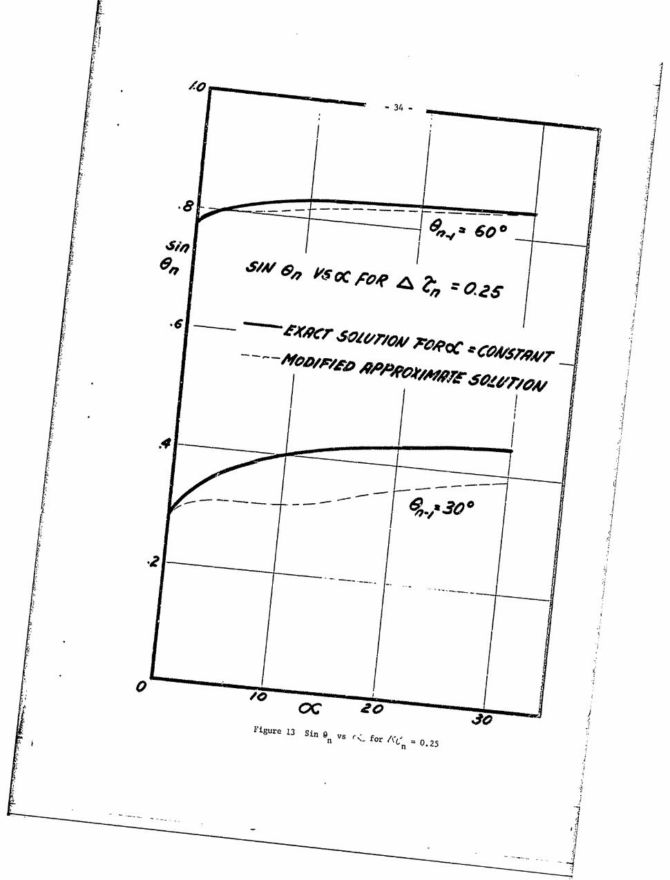
An exponential form for f(C) suggests itself, and it was determined
empirically as follows. It is shown in Appendix D that, for constant O
2~ (CC si 9+ +i 2 (Or 1) s
n (n- 4+ sin in) -dn ' +2 (2 C I) sin 0d'
0 0
(4.6)
Eqs. (4.2) and (4.6) were integrated numerically to obtain exact solutions
for constant C with which values obtained from Eq. (4.4) with different
choices of f(cC) could be compared. The final choice of f(rC) was
Se -0. 250 0.7 (4.7)
In Fig. 13 this function is compared with the exact solutions at =
.25 for en.I =300 and 600 over the relevant range of CC . f(oC) was
chosen to lie somewhat below the exact curves for two reasons. The first is
to take some account of the effeict of drag, otherwise neglected ir. this
analysis. The second is to relate to the actual constant-tbfst rcket
motors under consideracion, for which OC increases steadily fro gr.igition
burn-out. In applying the analysis to such motors, a mean value of 0C
k = " ( ( n-I + o ) (4.8)n n-
is used for simplicity, but this tends to make f(cn) too small, and Llnere-n
fore sin 9 too large. With sin 9 given by Eq. (4.4) and (&.7) .7 s ;n n
given by Eq. (3.13).
Xv,
-34 -
49- 604
At -
ri~ re 3 S~ n vs cK for A V 0. 25

- 35-
4.2 EVALUATION OF DRAG INTEGRAL
Since the drag velocity decrement is a small fraction of the
velocity achieved under rocket thrust, the mass-aitttude relation needed
t9 determine it can be based with sufficient accuracy on the equivalent
zero-drag trajectory, with sin 9 = sin 9 . Eq. (2.1) can be writtenn
dV dmm dt- b t m sin (4.9)
dn ntOn multiplication by - and integration this givesm
I _j_ dh - nm( V Vn i n g sin 9 (t t (4.10)
dtn-I i n n mn-I-
si n n-ln
n
nn
A second integration, using the motor burning relation
m =mn b n (t - ~ ) (.1
nsn 1 n-I -
gives
(V + V sin 9 V. sinn- n nh = h n . + b n( ram- m + n m lI n m n
2g sin 9
n (m(nI +Vm) (4.12)21b
n
In Eq. (4.12) it should be noted that the last term is very small in compariso
with the second term on tie right side. Thus, their ratio is
g sinl 9 n( - M) g sin 9 n(t -t n- ) 2
.= Order (10)2b n (Vn. + Vjn 2(Vn. + Vjn
using typical values for the parameters. Accoidingly, the last term can be
neglected in the expression for m for use in Eq. (2.11). The remaining ter-ms
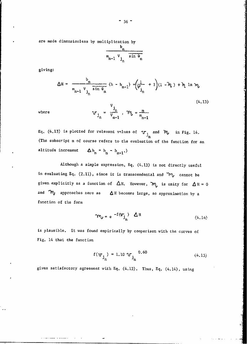
" 36"
are made dimensionless by multiplication bybn
m V. sin9n
giving:
AH = n (h 1h1 ) = - (1° +' In W
mn. V. sin 9 -
n-ln n n
(4.13)
where = , =wr in Vn-I
mn-i
Eq. (4.13) is plotted for relevant values of 'jj-n and "0 in Fig. 14.
(The subscript n of course refers to the evaluation of the function for an
altitude increment &h = h hl)
Although a simple expression, Eq. (4.13) is not directly useful
in evaluating Eq. (2.11), since it is transcendental and TM% cannot be
given explicitly as a function of &H. However, 'W6 is unity for A H 0
and lfti approaches zero as H becomes large, so approximation by a
function of the form
e e (4.14)
is plausible. It was found empirically by comparison with the curves of
Fig. 14 that the function
f(j. ) = 1.10 Vn0.60
gives satisfactory agreement with Eq. (4.13). Thus, Eq. (4.14), using

-37-
3e- i;Q(.3
4110
IIl
Figure 14 Altitude-Mass Relation for Zero-Drag, Constant-Thrust Motor
Ez- 38-
Eq. (4.15), is plotted on Fig. 14 for Ir. = 1.0 and 3.0, and the agree-3n
ment with Eq. (4.13) is seen ro be good for 7 greater than 0.3, the
relevant rAnge. Accordingly, Eq. (2.11) is put in the form
AVD (4.16)n 2m 1 sin 9 nn-l n
where h/Jn (a) :F(.17
hnh n
and "ft is given by Eq. (4.14) and (4.15).
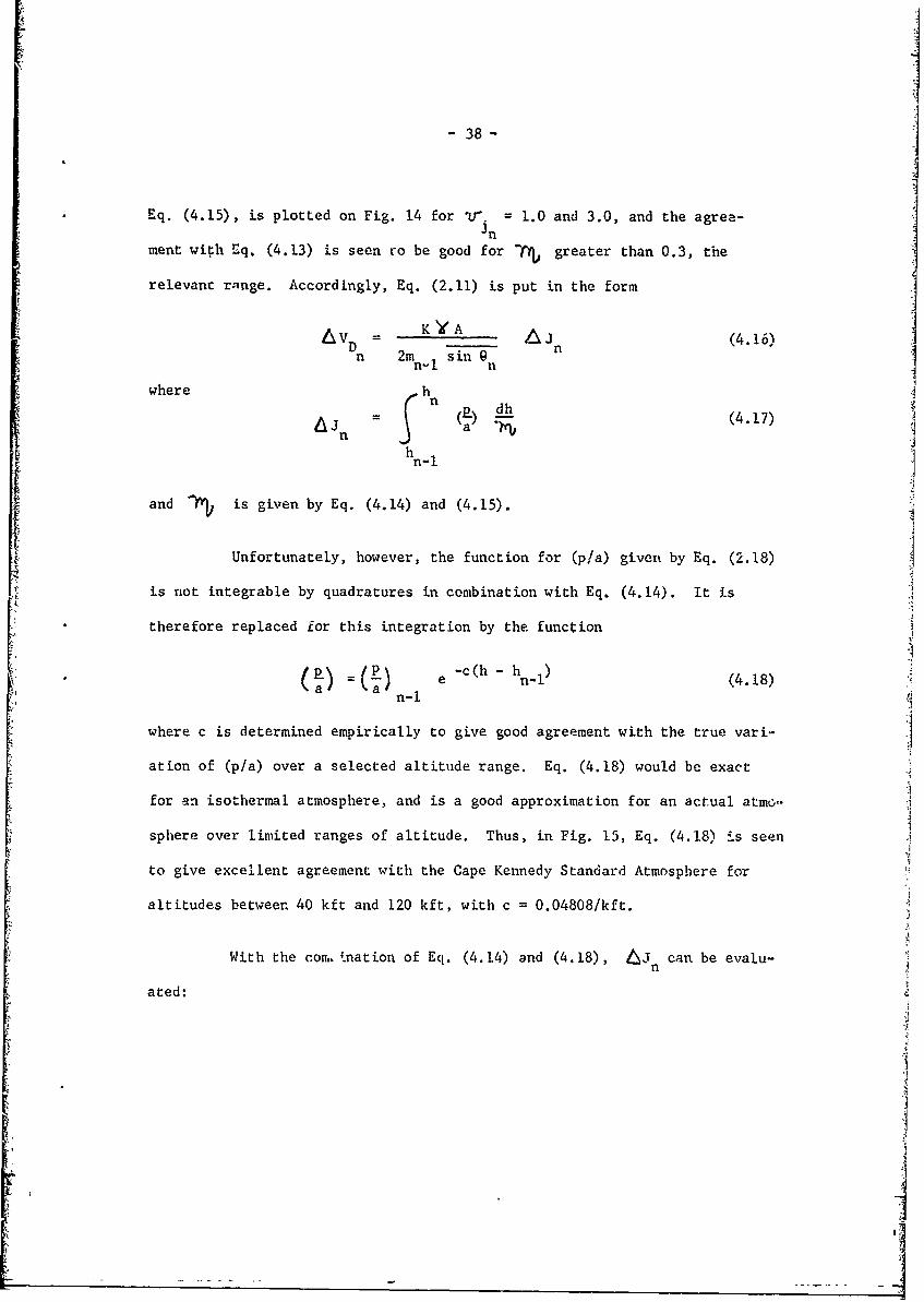
Unfortunately, however, the function for (p/a) given by Eq. (2.18)
is riot integrable by quadratures in combination with Eq. (4.14). It is
therefore replaced for this integration by the function
-c(h - h _)P- ) =--a e-h hn~l (4.18)
n-i
where c is determined empirically to give good agreement with the true vari-
ation of (p/a) over a selected altitude range. Eq. (4.18) would be exact
for an isothermal atmosphere, and is a good approximation for an actual atmo-
sphere over limited ranges of altitude. Thus, in Fig. 15, Eq. (4.18) is seen
to give excellent agreement with the Cape Kennedy Standard Atmosphere for
altitudes between 40 kft and 120 kft, with c = 0.04808/kft.
With the comn,nation of Eq. (4.14) and (4.18), 6J can be evalu-n
ated:
I
I
II

- 39 -
F ,!
(P/a)"c~
C -O.O#88O/kft.
, IiI
/Oq..
JILI
6 VV
Figure 15 (P) vs h for Cape Kennedy Standard Atmosphere
*k.t
4
- 40 -
h1. 1c + 1.10 bn (h-h
n n-1 e jrj 0.m40 hV n hnldhh n. 1 n n-I n-i nj
= a ). -
where i. 10 b n (4.20)n 0.40In mn' v n sin On
in n I n-i
4.3 DETERMINATION OF VELOCITY AND TRAJECfORY PARAMETERS
It is now possible to consider the evaluation of the net velocity
increment 6V arising from the effects of rocket motor thrust, aero-n'
dynamic drag, and gravity:
n F " 1 VD - V (2.3) ]
n n n
org h
Av= v &V v nn F D V + 6Vn n Vn-i n
using Eq. (3.9) and (3.10). This is made non-dimensional by division by
eVrn-v-I+- ~r ./k D (4.21)
n F 2 +,61TJ Dn n n
where
K '
n = l n" n - n , D = jK A (4.22)n n n 2m _I sin 9nn-i n-i n
K.
m I
igI

-41-
Solving Eq. (4.21) for Alnn
Alfn = + 12 (t 'F - D ) + + (AF n - (4.23)
n n n n
Eq. (4.23) reduces to Eq. (3.11) if ALr-F = 0 (no rocket thrust). Then
procedure for evaluating Eq. (4.23) is, however, different from the previous
one. In evaluating Eq. (3.11), Ah was selected and therefore L wasn n
given, and the time increment 1t was part of the solution. In then
present case, in which the burning of one rocket motor stage constitutes a
trajectory increment, the time increment 6t is known, as is the massn
decrement 6 mn so Lk~ must be found from the mass-altitude relation.
In Eq. (4.12) there is no need to neglect the small final term
at this stage of the calculations, since only simple algebra is involved.
Therefore, on multiplication by ,2 , Eq. (4.12) becomes:
n-l
/LA = 2-1Jn (n -(1 2 2 (4.24)
where gn- I sin 9
n V bn-l n
and H is given by Eq. (4.13) or Fig. 14. The calculation procedure cann
now be described. It is coovenient to introduce a parameter
defined by:
V bn-i n .2'
n-I g n 1
n-I

42
In terms of En-'
V. bn rV. 1 1 n-I 1 (4.26)0<= (OCn~ +oC-) = in n i +._l) n (1+ -i
n n-1 n 2g mn I m 2 +n
sin 9and nn= S'ni
A complete rocket-powered stage is calculated as one trajectory
increment. The known initial parameters are Vn-l, tnl, h n-i' E, ni Xn-1, g3
K, , A, mn_, bn, c, Vjn , (p/a)n. l t n is known, and this determines
t and A m V. and i, are calculated and 4l H is found fromn n 3n n n
Fig. 14. and R are calculated, and a trial value of sin 0Fi.1. n-I1nd n P,. sig [hi,
is estimated, based on the knowledge of sin 9 and .I Using this,
n is calculated from Eq. (4.27) and Ln from Eq. (4.24). f(Z) Iis then found from Eq. (4.7) and cos 9 is calculated from Eq. (4.5). This
determines sin 9 and leads to a new value of sin 9n. If this differsfrom the estimated value, the process is repeated from that point, using
the new value of sin 9 . Only the one iteration should ever be required.n
Next &h is calculated from &un, giving h. is ealculatednn nP
from Eq. (4.20) and used to calculate AJ from Eq. (4.19). This givesn
Si" from Eq. (4.22), and Air is then calculated, and AVtr isD Fn ndetermined from Eq. (4.23). This gives L V and V . .ange incremert *n n
AX can now be calculated from Eq. (3.1') and this gives range Xn, com-n C
pleting the stage calculation.
As an example, the method was applied to a Martlet 4, a g--
launched three-stage rocket, from launch to burn out of the se.:ond stage
(the remainder of the trajectory is high enough to require considerat iu, o..7
*1
43-
the g-variation). It was launched at 6.000 kfps at an elevation angle of
33.00. The first stage motor was ignited at 40.0 kft, and the second stage
motor immediately after burn-out of the first stage. Three alticude increments
were used in calculating the glide trajectory before ignition. In Table 2
the results of the calculations are compared with the output of the standard
HARP Computer Program for the same example obtained from Ref. 4. Vehicle
parameters and trajectory calculations, and the output of the Comz,.uter Prcgra,
are given in Appendix E.
TABLE 2
Martlet 4 Trajectory Calculations for HARP Case 1046
V X h t 9n n n n nkfps kft kft sec o
Launch 6.000 0 0 0 33.0
Stage I Ignition HARP 4.822 67.2 40.0 14.61 28.92Present 4.808 66.4 40.0 14.67 28.8Error -.29% -1.34% - +.41% -.42%
Stage 2 Ignition HARP 12.155 174.8 93.9 29.61 26.02Present 12.21 172.8 97.1 29.67 27.7Error +.45% -1.14% +3.41% +.20% +6.467,
Stage 2 Burn-out HARP 18.621 311.8 158.7 39.61 25.35Present 18.84 306.8 166.9 39.67 27.3Error +1.18% -1.67% +5.16% +.15% +7.69%
i"
-44-
4.4 DISCUSSION
Table 2 and Appendix E show that rocket-powered trajectories
through the atmosphere can be accurately and easily calculated by slide
rule by the present method. In the example the velocity and range at
burn-out of Stage 2 were given very accurately, the altitude and elevation
angle less accurately, both being too high. The time was of course given
accurately, since it was known except for the initial glide trajmctory.
The high values of h and 9n, although acceptable, lead ton n
over-estimates of apogee, or of orbital height after Stage 3 firing, and
this suggests further work in improving the method of determining sin 9,
so as to decrease its value towards the correct one while retaining a
simple dependence on the relevant parameters.
JI

- 45 -
5.0 HIGH ALTITUDE AND ORBITAL TRAJECTORIES
Rocket-powered vehicles will in general reach very high altitudes
or go into earth orbits. The upper parts of their trajectories must then
be calculated by recognizing that gravitational force is a central force
varying inversely as the square of the central distance. No aerodynamic
drag need be considered unless such problems as the gradual decay of orbits
are being studied, and any high altitude use of rocket thrust can be treated
as a constant-g problem using an appropriate value of g, because of the
short duration of the firing.
The problem then becomes that of determining zero-drag glide
trajectories under the action of an inverse-square central force. The
basic equations governing this motion are simple and lead to explicit
solutions for trajectory parameters, so there is no need to seek even
simpler approximate solutions. In this section the usual solutions are
merely derived to complete the set of trajectory equations. No examples
are worked, since the solutions are not new.
5.1 EFFECT OF EARTH ROTATION
In previous sections of the report, trajectory analysis was
given in terms of vehicle velocity V relative to earth. This was suitable
over short distances for which gravity could be considered a constant
vector. When the true central force nature of gravity is considered, theI
trajectory analysis must be based on the vehicle absolute velocity of
magnitude U, or in vector form:
E
i I~u

- 46 -
where UE is the vector velocity of the earth's surface at the gun muzzle.
Since UE and Vare in different directions, it is convenient to express
relations between components. These relations, in the context of this
report, would be applied at the point on the vehicle trajectory where the
constant-g analysis of previous sections is replaced by the analysis of
this section. The relations can be obtained from Fig. 16. First, using
the cosine law:
U2 V2 + UE2 + 2VUE cos. (5.2)
But, from the right triangles of the diagram it can be seen that
V cos 9 cos Yv = V cosX (5.3)
so that, cancelling V and substituting for cos-in Eq. (5.2):
2 2 2U = V+UE + 2VUE cos cos (5.&)
where is the azimuth angle of the gun. Eq. (5.4) gives U. Thev
absolute path angle 5 to the local horizontal is given by
U sin 6 = V sin 9 (5.5)
The absolute azimuth angle u is given by
U cos cos V Cos os v + UE (5.6)u V
'7

- 47 -
5.2 FUNDAMENTAL EQUATIONS AND SOLUTIONS
Because only the central force of gravity acts on the vehicle
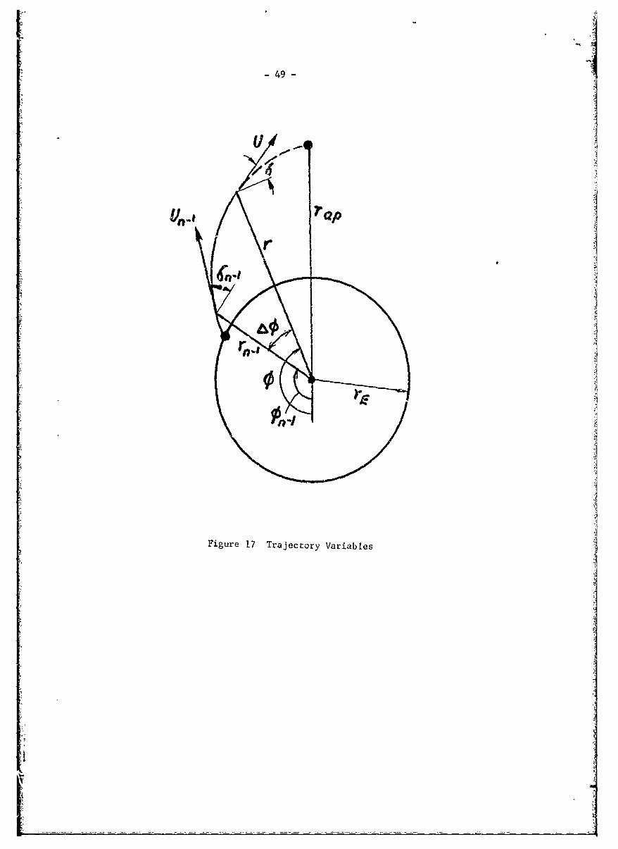
its trajectory remains in a plane passing through the earth's centre, and
Fig. 17 defines the variables of the trajectory. The equations of motion
of the vehicle for the r- and 0- directions are written, for unit mass:
r-direction d 2r dO 2 rE 2dt---e____ - r ---) E (5.7)dt 2
________io r LL-+ 2 do0 (5.8)0- ir ct ondt 2 dt dt
The second termb on the left side of the two equations are the centri-
petal and coriolis accelerations, respectively, and gE is the value of g
at the earth's surface, used in the previous sections of the report.
If Eq. (5.8) is multiplied by r, it can be written:
d (r2 dO -
d F)t
or
=2d - C, constant = rU cos 6 (5.9)rdt
where C = r Un_ cos nl (5.10)
ded- can be eliminated from Eq. (5.7) using Eq. (5.9):
d2 r C 2 rE 2
dt 2 r3 gE r
Now, dr U sin6= U . Thereforedtr
2 dU dU 23 g. r2dr rr C (
2 dt r dr 3 2 (5.12)d 2 dt r r
-48-
IZI
Figure 16 Veicle Vel6city Diagram
49
' Il
p
Figure 17 Trajectory Variables
fI
S- 50"
* • Eq. (5.12) can be integrated directly to give
2 - C2 l---7- +i " 2gE rE21 (.3
2 . U = (nl i ) 2(n- rUr rn. 1 rn. 1 5.3
?Since the altitude change of the vehicle is of primary interest, it is
convenient to introduce
AT=. __ - n (514)r
r
In terms of AhU, Eq. (5.13) appears in the form
U U 2 2gr2 U2 (2- U (5.15)r r 0n
whereU U cos60
At apogee, U - 0, so that Eq. (5.15) can be solved for p :r ap
ap g + ~tan 2 6n- (5.16)
%r )- Jr U - r
n-i 0n1 n- i
Eqs. (5.15) and (5.9) determine vehicle velocity as a function of altitude.
It is necessary to relate altitude to elapsed time. This can be done using
dr r 2 d 6hu r rnl ddt = d rdU '2 (5.17)
r n-lr (l -Ah) Ur
Eq. (5.17) canbe integrated directly, using Eq. (5.15), to give
- 51-
r Fn1 1 22- 2 - a]
n-iS a n-i (1 -, an - {rn:UO2
2 2n- 22
2S + - 2 (1 -Ah)O f-2S + -gE
gErE 2 rn U 0 n r n. I U0
+ grn-In-+-U3S 3/2 sin'l ( -(i- hI) s in"Q "
UOn-1 -e (5.18) -2
where S = E L - sec2
0n-i 0n-
r 2gErE2 2V tan2 n- + n-i n-1 - 21 (5.19)
In order to find the range of the vehicle, it is necessary to know the
change in 0. This can be found using E:q. (5.9):
d_£ d Ur Cdt dr" r=r
Therefore
dO Cdr C d u (5.20)r 2 Ur rn . iUr
Eq. (5.20) can be integrated directly using Eq. (5.15), to giveI 2 ,& h ,++ 2 , .gErE-v - 1)
40 = sin " { 2 n-i n s rin12( gr 2 -
Q
(5.21)
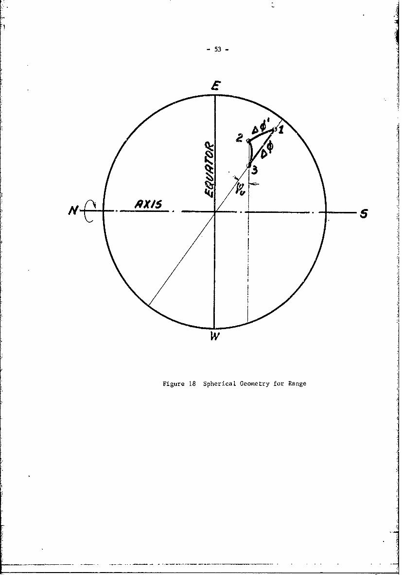
Referring to Fig. '8 the vehicle range increment AX is the great circle
distance between the point 1 intercepted at time t ac the earth's surface
by radius r and the position 2 at time t of the point 3 on the earth's
surface intercepted at time t by radius rn:
" 52 "
AX e 0 (5.22)
A 0' can be obtained by solving the spherical triangle 123. In thLs,
,A0 is known from Eq. (5.21), & is given by Eq. (5.6) and great circle
arc 23 and angle 231 can be found, since the latitude of 3 an' the small
circle (eastward) distance 32 travelled by point 3 in the time A t,
given by Eq. (5.18), are known.
*1
--
I-
-53-
Figure 18 Spherical Geometry for Range

- 54 -
REFERENCES
1. Luckert, H.J., "Report of the March 1965 Test Firing Series - ProjectHARP", SRI-HK-9, Space Research Institute of McGill University,July, 1965,
2. Daniels, G.E., Scoggins, J.R., and Smith, O.E., "Terrestrial Environ-ment (Climatic) Criteria Guidelines for Use in Space VehicleDevelopment", 1955 Revision, NASA TMX-53328, May 1, 1966.
3. "Ballistic Tables, Martlet 2 Vehicles, Vol. 1", Space ResearchInstitute of McGill University.
4. Bull, G.V., Lyster, D., and Parkinson, G.V., "Orbital and HighAltitude Probing Potential of Gun Launched Rockets",R-SRI-H-R-13, Space Research Institute of McGill University,October, 1966.
- - + . . .. .
A-I
APPENDIX A
Trajectory Equations for Zero Drag, Zero Thrust, Constant g.
Newton's 2nd Law for X-Direction (see Figure 1)
9h
d (m dx d-X 0(n -) = 0
Thee fredt dt dt2 4Therefore
dX cnstant -V cos n V cos 9 (A-i)
and AXn = Xn - Xn = Vn_ 1 cos 0n. I (t - nl) (A-2)n ni -i -i n n-in"d
Newton's 2 nd Law for h-Directiond dh) md2h
-rg = d (m = m d constantdt d d-t
There foredh = V sin - (t tn)=V sin 0 (A-3)
and6hn hn hn-I = Vn.I sin 0n-l(tn-tn-i)
- 4 (t - tnl)2 (A-4)
Introduce= 2gX 2gAhn
nn nn A5V Vn-i n-i
and substitute for (tn - tnI) from E4. (A-2) in Eq. (A-4):
n= tan An YAn - 1 sec 2 ' n -1 n (3.4)
uLu dividing Eq. (A-3) by Eq. (A-i) an expression for tan 0 is obtained:
g(t - tn- )tan G tan 9 n.I -lcsQ (A-6)

A-2
If n is set equal to and (t n - t 1 ) is elimated using Eq. (A-2)
the result can be written:
tan n = tan 9n. - 'sec 2 0n-I &n
or
2(tan en-I tan gn)4)(n (A-7)
sec2 "n-1
Again, if Eq.(3.4) is solved for Un' the result is:
2(tan 9nl -tanZ ni - c2seC2 Qn I A )
sec2 0 n-l -
On comparing Eqs. (A-7) and (A-8) it is seen that
tan Qn = tan2 )n- -sec2 Qn- A (A-9)
With a little rearrangement, using trigonometric identities, this can
be put in the form:
n - COS 0nsin n - (3.5)
or Cos 0n~Cos 0 -n-1 (3.6)
2gIf Eq.(A-4) is multiplied through by the result isVnlIsln Qn-
V n- n \= ( Vnsing, Vng t 2 (A-10)
n-ls' Vn-n-12
A-3
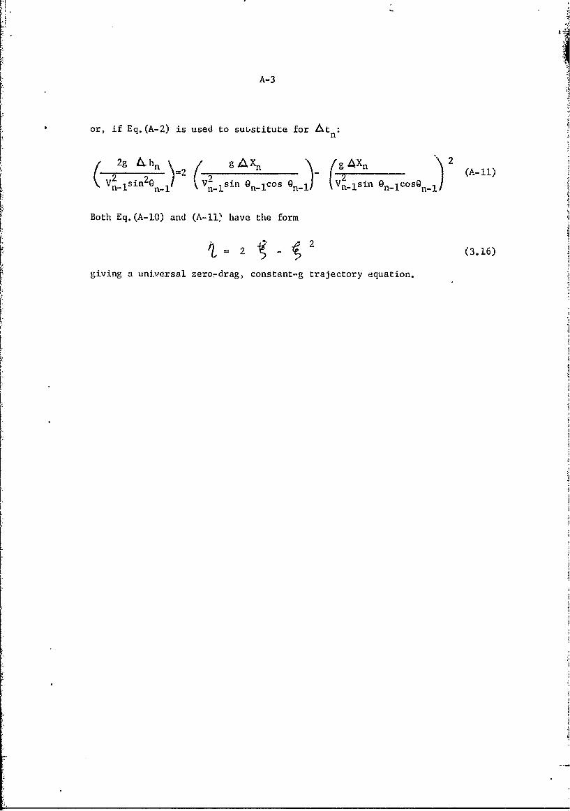
or, if Eq.(A-2) is used to suustitute for Atn
2g L. ) / gA X n \ /g Xn2- - 2 (A-11)
s i ni V s i n 0 n ~ C O s Vn ) ( V n s i n @ n l O S n ) l
Both Eq. (A-10) and (A-1Ia have the form
giving a universal zero-drag, constant-g trajectory equation.

B-1
APPENDIX B
Calculationi for Martict 2A Shots
0 tn ~CJ 1 o r-..10
0 -
-4 C
C: m -4 C'u 444
coa %* 00
44 ..4.44CCs 4 C'
r--4U. 00 0 - CI5 lO0
0 sI .~0 C td N N
5-4 o C,Sr1-1 4 is '
o4 0*0 Is .. 0 oco
s-4 9-4 Ic!r as-!F .-4 N- C4 4 a qN mcn is
LM U4 o connO
N4 .4 7-n-
01 co co It 0O
*l0 or sF4 CNsO~s00 ~ d. ClO5
50 I'-C 0450 0 C 0.4~ CO 1 , -i404 is. ro r, £l 0 COs CCJ N M04 'C .0 000- kn C
CO .d - .4
C', Js "O' 00 00 %05005 c cNl 14 NCO
Si C ~ -4 It -o 0 t
0 r co II IT 04 )0. 1 : 4t 0
o'c to IC os U s Coa l > I 4r
4 0 0i N4 >- d
4t-> COC
o 4 Lo N A0 CN CO
O4 0, C 000 '4,o .0 r.
Cd) CO '1 '2 -
CO 00. CO 0 15is Cii C1s4 . 4 0 o 0 0 . eq
44 co co 044 0 00
s 0 *l N 1.4 c
-d 4l 0 C
to. 0)c o10
44 d 4 dU 1 00
'2 '2 0 0Jd 4 .. N N 44
e- C, -4 00
d 0)dO 0 0000A
'4 1 wCOo
to 0 0
- 00 0
4C 0
0 0

B-2
C4 LA N %0
cc 0 % 0 o c41 A4J ci
0 I to I -1 c l
f:~ cc cc r, 0%X.4. 144 0 o 0 ITco
co to
44 c . 7 l cc c
0.0 ca
-4 CCI -%M
&j 'W In rI,~a 04a 4W~.C I (.4 o -%
(.4 4
N* o 0% In c cc4) cc .- C' (1 lo0a
w v% o 00 n -4
lo lo r, cc . -ol
(n (A 0 -
c: 0 0
cc r, ca -c cc on *l 04 (A T.444-i 0.4- 4j .c . . .-4 N .A .
-'i m ~ L44 .44 CIr )0 iV
N--cc "i -4 l
(n4 a. 4j a'ccc cc ccccc-VtU40 n4* l w! o~ co
0 c~ 0 - -4csn
0o I. cc NoI l0'~ ' o -40--c -o U cc'I.
U4 ITN 171z -o ~ ~ ~ o 4-' N--.'b .77 ol-a
cc v! 4
v) U oI U~ n cIC s lc)(
.- 4( 44 .00 Of _ _ _ _ _ _ c
A C I 0 c4_ ________ n
1 4 c z 4- . -) a,4 a% *l
a4 0 444 (nl aNc)L
.7n (A 1- a4 0.r-4N1-
:3 .7 1-4 cc, cccccc*~c 0(0
0 o N I&L N %D i * >
0 I 4 l .I I NcV1 D ccu.. coco Q4 U *
M-- N. a .
N Cn (1 a, a, t
U a cc cU Tooc4
04 It- -
N7 4 a 00
t" a 44 -44-40c
r41.-4 r., -W 0:
u 0 .,1
I> -1 -

B1-3
0,0
1- X~ '. Of: 4 10 ro4x -4 o 0.- f N 04% '0 0
4 ' 0 a, 41
anC C ~aj ton .0 co v 0
0a' a,
'.3 -a1
.4 .> 0. -AI T4 -C7 ~4 C% 4
.i~ ~~ ~ -a. - tC .O 0, 0
or, ct. 4t 4l In40'
Nq 4,4~1-C.
C- N. _ _ _t _ _-
I In 140 ~ ta t4
4~ 44 r<X U.4.4 .
4 n 06 .1t 449
14 44 0U r 4 N 4 A . .44N ~ .anJ 44 ?C 0. 0 .n CS
-4 .4 - 04 Ct. Ct. CO k0 V0 %
r t. H1 C64 MI* N N 444 C-b.- 0 4n0,.11 IT IT x I4 .0 .. ' CZ-4et
4 ir .4 V;C!
4o ct.0-A00'0 n cN 0o N4 0 %0e T N
a~~~~ C4.. * C.I-41.'Z'0 > II 0 a TaTC 4(In NCC 4C Ct.4 0'CJ
0 00 00 OOS a . 4. .440~~1 . C.a a. a t
44' -q - 44 OLJC4 oo_ o__ane N,- .i4 N-a (n :t '0-t c
0 ~ ~ C co4 OSOS 0c. CC t 4 . .0 .0.0.1 a 0'3S 0 00 >,C-'r"N4O t..0 t
Wa an ) aY ct. m- 0n in -A oD n ct
a4 !at 4- oat N1 U IT
44 4 .0 aA4 wl L4 ca" . 40t. 0t
O) c: %0 .0% ,-a -a 04 N0O0 140 0%m0 C 0A.0 ID ON Nl ,0 q4 % n0%D0C
. 0 0 (n Nn4r CJClC
-4 9) (n *. N 41 0 u. g N 0 3
.0 0 :0 li( - n N .-a0r,0Ian ana.- 4
0 0- an 0CC 0l Nf
34~k at.-4 44 CIO44a 40C O.O~ 0 N~. .I I ~ . .
N~ _ __h 0
44~ 0 "
n an C) o 0 0 F__ _
4C 0. 0 CO0 n 1$4 N . 44 0T co 0 ,o
0 .(.1 . 0 .- . ) 1-uC! C
12 Lncl 4 i -n 4
4 &J 1. 0 41 4
Ct. Q 0 an anCi 0 ~ J i .4 0Q
ano anA
II anU.
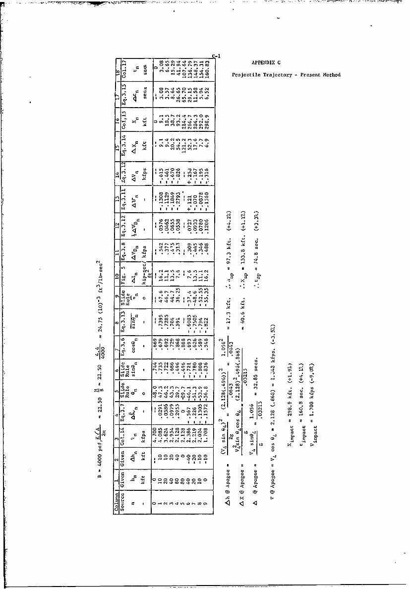
00 AC, ' 1 0 r, CAPPEN'DIX C
w -4 T1 0 cn) T nf B Projectile Trajectory -Present Methodo) , 4 4 -4 . -4
C-4,1 0n 0 In CO ITAO 114
CI 1 0 C4-
-4L , 4Tr J-t cn 9 0
IiC X '4 1 0%C% 0-T 4 C4r-f-.'3-4 C. .4 .2& NA 'n~4
-4
* 0 LA 10'
m >4 'IS '0lN, 10 m
0' <32 Il I + .8
cn 0 CJ 'T C r, 1I" C1 -4C , CSf OI
'0'J0( r'c-0
4 C 1 t00 4 (n0 C 4 a, 0 1 0-t~ 'M (n 1 4(nO0 (
Ii Ci II U00
144
V" CIS -4"' '4'
-4 M2 .2ID-1
-4I In A(
'.1 I. IT 17I n l T nIUS C4 1 1 1 1
.0 I ,0 ' C 0 It0IS0
a) 11 1 a, ID ID ON vi w 1 %0(N 0 ______ .' ' 1 0 -
0 a,( * N I
LA CJ 0 1Cs s0c.' %D 0 0 'to 10 ISUfCD 104q~u u u g' N ~ 2 0 .
I-4 -40 U -A N . .0 .- . . . . 0 O 'CI (1 C4 'A's s sb c's CI 0-n 0 0~C4 10 01 m . *)
R . NT 00* I
In A 4. C:4 c4C!I!41 : "T( 0 00 - n ,mN(0.. -4 fn '-7 00 0
0 rd -, 4 -. 7 7 .SN 11 1N n nN.- C- . N . ..4 *.%.. .. . . . . . .N 1 0. 12 C2
In InI: I
CIS~~I U4C117 N
CIS IT (000 N400 n IS 144 0. CD O. 04. OS 2
-4 Cr. . . . .~ 14
H2~~ R 1 3

- .P C'' I' 2~Cl) N
* ' N ~ tn~ 0 C U' L ' -
~~N C' "-%
I- t.-1 N
Z. CO.-'
ON IT In
L - cc'0 -? f"N CO'- 0 1- C r- Ct
Lu -
It.t N nr-i .A~ V) L ,'
LM U -N
0- 0' .
0w 0 , p- o.OO~
i -j 0i co , c N * 't -4 M~
L0- 0j rIt 1 0t -t -t .f V0..................................................................
to .0 o C
w0 WJ 0-i -1 C' 0-~-1
04 LI..J0
0J uu N 'AJ 00% C>- n -4 %n$/' l) W N 4 4)SN
ej -2 0 u~~-' -1. rt N L...- -'NaN0%
i 0000 00
zi N NN N) 1~ ^4 OF-' U-
E W >
_u 0 I' * 00 In C
D-1
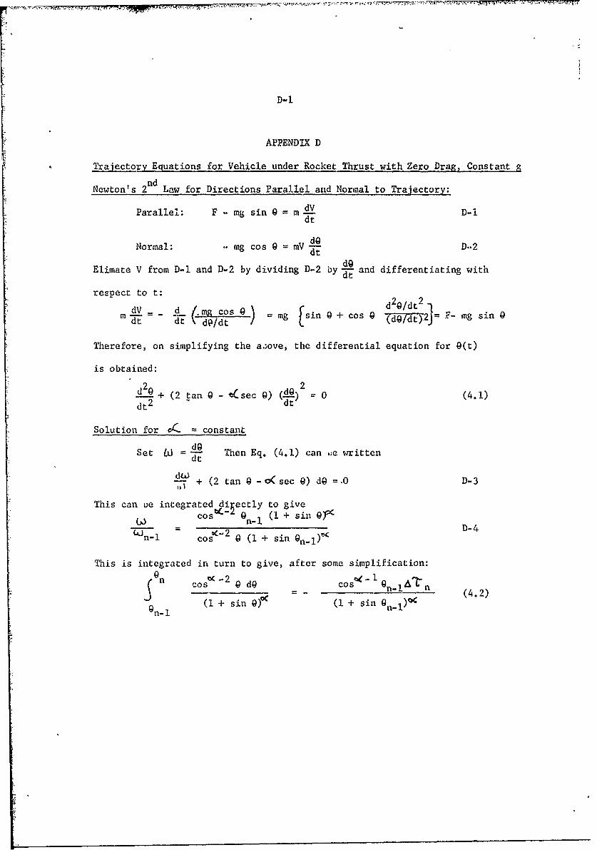
APPENDIX D
Trajectory Equations for Vehicle under Rocket Thrust with Zero Drag, Constant g2nd
Newton's 2 Law for Directions Parallel and Normal to Trajectory:
Parallel: F - mg sin 0 = m dV D-idt
Normal: .mg cos 0 =mV D.2d
Elimate V from D-1 and D-2 by dividing D-2 by d and differentiating with
respect to t:d2G/d 2
dV _ d C.mgcos mg sin 0 + cos Q (dQ/d)2J= F- mg sinOdt dt \ dP/dt 9 S1
Therefore, on simplifying the a.;ove, the differential equation for Q(t)
is obtained:
d20 + (2 tan 0 - t(sec 0) (dO) 2 0 (4.1)dt2
(4.dt
Solution for ( = constant
Set LO Then Eq. (4.1) can .e writtend
,, + (2 tan 0 -o<sec 0) dO =O D-3
This can oe integrated di ectly to givecostM 0 n-l (1 + sin D-4
n-i cos 0 (1 + sin On-l)"
This is integrated in turn to give, after some simplification:
n Cos 2 0 dO cos O n- !i ' T n (4.2)
(I + sin 0) (1 + sin On-1 ) 40n-i1
D-2
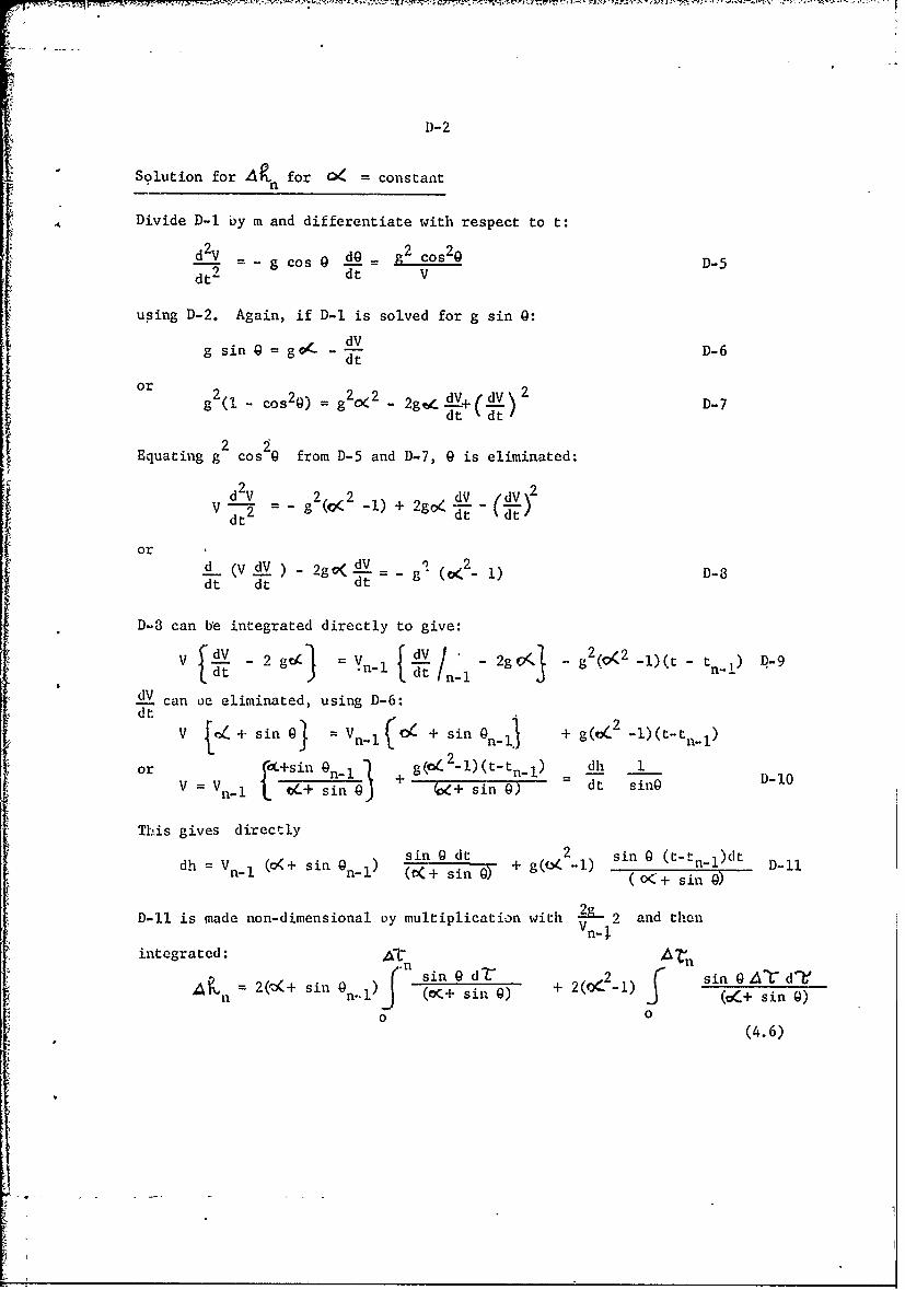
Solution for An for O = constant
Divide D-1 by m and differentiate with respect to t:
d2-g-v dg =-gcos9 __ Cos20 D-5
dt2 dt V
using D-2. Again, if D-1 is solved for g sin 0:
g sin@ = gc-- - Vdt D-6
or 2, 2@ =D2-7qg (I - cos 2 ) = g2 O 2 - 2 dV ) 2 D-7
f 2 2
Equating g cos2 0 from D-5 and D-7, 0 is eliminated:
dV 2 2 dV (dV 2
dt 2 g dt)
or
d (V dV ) - 2gv( -q = - 2 Ddt dt dt g ( -)
D-8 can be integrated directly to give:
V - 2 gg c4 n, tg/ 2g 0< 82 (0,2 -1)(t - tn D-9
dV can oe eliminated, using D-6:Vdt V sin 0 = Vn-l(C4 + sin @n-l1 + g(OC2 -l)(t-tn_l)
or G+sin 0nI g(. - tn dh 1V = V n. I ck+ sin ( 6- + sin 0) dt sinO
This gives directlysin G dt 2 sin 0(t
dh = Vn I (o<+ sin n. ) (sin 0) + g(O i n 0 tn-l)dt D-11dh = V 1 (o( s n-1) +Z sin(-1 (n-)dQDl(o<+ sin 0)
D-11 is made non-dimensional oy multiplication with 2 9 and thenVn- -
integrated: AT TZnjnsin 0 d( ) sin 0 A-d2
A = 2(o(+ sin 0n ) (or,+ s 2) f_()osi + sin 0)o 0
(4.6)

E-1
APPENDIX E HARTLET 4 TRAJECTORY CALCULATIONS
Comparison With HARP Case 1046Parts I, II, III- Constant-g Calculations from Launch to Burn-Out of Stage 2
7. Errors from HARP Case 1046Vn Xn h n t
Ignition Stage 1 -. 29 -1.34 - +.410 -.42
BurnOut Stage 1 +.45 -1.14 3.41 +.20 +6.461BurnOut Stage 2 +1.18 -1.67 +5.16 +.15 +7.69
Q) 7W
-t-
o .C
co~0 co~
.. . . . . - . .. . .i
"V.. . .n nN'
.0
0~ Cr
,- I.T
o .. . ... X
0 04 .. C'w caC' 0 .. ??. * C. N
. 0 -I4 -t , . .
00o
00 06
0. 0
; . . ... .C .. .
-rC 0. 0
C' 01d N< , -
0 0 - k"
.4 04 .4 U 00 - -
o o -C'7. .... .. C..n
.3n. C, t t~ a! C !
* .44 N N 0 - 0 N C'. N
S, U C) .0 .0
o r %0 100. i: CD. w0
,- 41N
>4 a) 'd a, 0 . 10. N v 1 . 0 * C OC)1c CO -O C! C!n - 0
O t .0 C.,
a - ° n- .0 n
U -. -. * 4 .,.2 .
0 CIO r;'4 .N N.-0 C- M 1
C; . 0
N0 X .. . .. ' C 0(
74.1 01. -M ~ '-. - ; 0 4 - -'U0
N04 *,-? IN% .0C N w
' 0I IT 7 I - C
Z5 >-~, 00(0
('7 0.0.. M "4.4 CO - 0 -, 31 c
4 C: 0.0
'T N 0 7( .3 . * . .(P 0 1 n t I ..I - 0. 0. w.
*4 0' 0 14 4r I 0004 7. - 0 -1
-4 co w V . . 10
0 4 . O M.0.40
*-44 C .?.L . C' ..
0.0 0.
In ' ;o.4;4.0 n Ia.In
0 .4 $4 7(. 0.d0 C - 1, 40 0 - : = Z0 C11 a- CIAN M 0.. 0 00
0 9: 0' U' ~'* rOq U0 0V.
31n C) I *. . .2 4
., 0 000 T' D. C aC
o 1 4 V.: Ca CS a v
CO n. V)N4 CrV U
00 .0 0 N .3O~~~ 'n3..01-

-~c' C~. I A N ~-0 0 (11
X Ao fA Al 11 *. C, 1) 1: 8
i: CO IOC 0 0 0.CI CIa
0*1 fi) to.. c 00000' 0 0
C f O N0 c "INI
In 0. ~ ' 0e M4In IN 0VA. r .j C-3 Al CAIN I~- 1: ,0'0 4 '.0
- f) P.M N N JCj(VAl Cl (cl0
-j N C'0 ,I 1 C, Ur~-'O C-) mNUS C , 0 A IN A rl * 4 0 M
CA1 M (n eq IN .A t'CO- 00
0 In .A (" q* A * * 4 A ,
- 0 1,10 OVC Il A-A -6 AML%coA 3 4 l 08 AA
tA N , IN ( N -4 -i
MA -4*,a-0000tOOO
A '.0 1C 0 C. 0, 0
N -s * OO .4 0 I'D0 00 1.% LA r C (A 0.4I P,
IN * 4 N N 1 A 4 A-1
IN a") <0 U% C-. 000 N In -14 *0 LA- M00
Nl CL.0(IOOO 0 CO 'o M~ NA. 0 0 0O.0 * C 000ON U. 10 NIA lAJ N CO 4C). .I'.'%
~0 CO I- -I IN000 4 -4J~ -tNo t-'~A
m ww 0 jI ,u0 -) .A '2 0 ) t 0 0 '.0 U
4 C.'000 N4I CA
0 - In .0>ZO. * r A. .0. . . . .11u. . A z'
0 '0 n IV-
.C-~OO0 .% .o -4~ 4'. ..C) U ~ .. 14- -I.O
>4 -. 4 (A 7* I- O I- IN C) 1.5Ij ku 1-'4 .'.11, .4 %,:4 .
-!j u. 0..A .4 -. Xi'. ...1. M.* 0 * *.)-- '*' ~~~~- n eAIN~la -00C ' ~.
Ij U 4c, O 4
A J.
UNCLASSIFIED
Sec, rity Classification
DOCUMENT CONTROL DATA - R & D(Security classilication of title, body of abstract .nd Indexing annotation must be entered when the overall report is clusailled)
I. ORIGINATING ACTIVITY (Corporate author) 12a. REPORT SECURITY CLASSIFICATION
Space Research Institute of McGill University Unclassified
Montreal, Quebec, Canada 2b. GROUP
3. REPO4 TITLE
SIMPLIFIED FORMS OF PRELIMINARY TRAJECTORY CALCULATION FQR GUN-LAUNCHED
VEHICLES
4. DESCRIPTIVE NOTES (2
ype of repoti and inclusive deice)
S. AUTHORS) (Fit.: naMe, mtddl. Initial, last name)
G.V. Parkinson
6. REPORT DATE 7a. TOTAL hO. OF PAGES 7b. NO Or REFS
August 1967 75Ba. CONTRACT OR GRANT NO. 94. ORIGINATOW'S REPORT NUMDERS)
DA 18-001-AMC-746 (X)b. PROJECT NO. SRI-R-19
RDTE IV014501B53CC. 9b. OTHER REPORT NOS) (Any alflin n m ,re Met mx be .aedad
thia report)
d.
10. DITRIIUTION STATEMENT
'hls documnnt has been approved for public re1ea,and sale. its diztribtio is unmi.tted.
11. SUPPLEMENTANY NOTES 12. SPONSORING MILITARY ACTIVITY
I J ~ lsearch & Development Center.
* IS. AUTRACT j e02- Reoutn& Qmai, Md. 210Q5,IS.,ASISTRACT
'An approximate numerical method for calculation of trajectories ofhypersonic vehicles is described, with particular reference to gun-launchedvehicles. Because of the form of the hypersonic drag coefficient, arelatively simple calculation using functicns which depend only on altitudeis possible. Reasonable accuracy can be obtained even for computations inwhich very large calculation intervals are used. The method is particularlysuitable for preliminary engineering calculations which do not justify a
detailed computer solution, and has the added advantage of giving the analyticforms linking .input and output. The technique is shown to be applicable toglide trajectories with and without drag and to rocket powered trajectories
as well.
0169PLACCO 0D FORM14711, 1 JAN $4. WHICH tol
DD o 100VSol473 ::oLUw i. ARM U a. Unclassified
Scurty Cl,-ifcation
_ F it Security Calfcto
! 14.
EROL WT HLZ W LI W
Hypersonic DragBallistic TrajectoriesGun Launched Vehicles
IRocket TrajectoriesGlide TrajectoriesOrbital CalculationNumerical Trajectory Computations
UnclassifiedSecty -Notification
Recommended