Proceedings of the International Conference on Industrial Engineering and Operations Management
Washington DC, USA, September 27-29, 2018
© IEOM Society International
A Two-layer Time Window Assignment Vehicle Routing
Problem
Mahdi Jalilvand
Department of Industrial Engineering
Shahed University
Tehran, Iran
Mahdi Bashiri
Department of Industrial Engineering
Shahed University
Tehran, Iran
Abstract
This paper presents a two-layer time window assignment vehicle routing problem (TL-TWAVRP(. It is
assumed that there is a predefined time window determined by the customers which is called exogenous
time window. Also, there are two-layer endogenous time windows inside the previous one. The outer layer
has bigger width and the difference is a violation variable. These new time windows give a flexibility to
career companies for visiting customers after the end of assigned time windows to perform services to more
customers. If the vehicle arrives at the customer in her/his inner layer assigned time window, no penalty is
paid but if vehicle violates inner layer, a penalty will be calculated in the objective function. No extra
violation is allowed from the outer layer assigned time window. This problem is modeled as a two-stage
stochastic problem. The decisions of first-stage are assigning inner and outer layers time window to each
customer. Then in the next stage, routes will be planned for each scenario. Finally, by comparing this model
with the TWAVRP, it has been shown that the proposed model has better performance to minimize total
cost with serving more customers considering their exogenous time windows.
Keywords Vehicle routing, Time window assignment, Two-layer time window, Stochastic programming.
1. Introduction
In daily goods distribution network, career companies face lots of delivery from suppliers to customers that should be
cost-effective. In the classic vehicle routing problem, the total traveling cost is minimized as an objective function.
One of the most studied subjects in this problem is the vehicle routing problem, considering customer’s time windows
which are called VRPTW. In this kind of problems, each client must be visited in a pre-specified time window. The
VRPTW is a problem with hard constraints although in some practical applications time window constraint can be
considered as a soft constraint and the violations must be calculated as a penalty in the objective function. This attitude
converts the problem to vehicle routing problem with soft time window (VRPSTW) which is studied less than
VRPTW. The VRPSTW considers time window but the difference is that each customer can be visited at any time
and vehicle must pay penalty for time window violations.
1315
Proceedings of the International Conference on Industrial Engineering and Operations Management
Washington DC, USA, September 27-29, 2018
© IEOM Society International
In real-world applications, the customer and supplier might agree on a specific time interval for delivery that can
consider as an endogenous time window. Also because of some unpredictable conditions, career companies may want
to have an extra agreement with customers to have more flexibility with paying a penalty. The amount of flexibility
may depend on company equipment like vehicles’ capacity and uncertain distribution conditions like traffic condition
and etc., so the agreement with customers is determined by a two-layer assigned time window. It should be noted that
mentioned assigned two-layer time windows should be inside of a predefined time window which is called exogenous
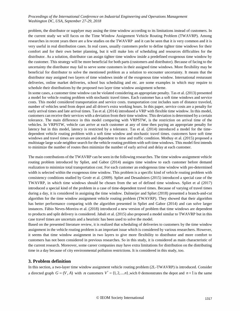
time window. As illustrated in figure 1, all of definitions can be better illustrated. In the real world, demands are
usually unknown, hence TWAVRP model is introduced for vehicle routing problem with stochastic demands.
exogenous time window
endogenous time window
outer layer
Figure 1: An illustration of two-layer time window
In this study, more flexibility is considered by assigning two-layer endogenous time windows. Suppose that a career
company assigns a time window for each customer before realization of demands and other uncertain parameters. It
means that the customer should be visited during its assigned time window while the customer has defined a specific
width for its assigned time window. In that case extra agreement with the customer including a penalty will make
distribution more efficient, so in the current study inner and outer layer endogenous time windows are assigned in a
predefined exogenous time window as the first stage decision. Then routing decisions are made based on the first stage
decision after realization of all uncertain demands. In some cases, paying endogenous violation penalty cost is more
cost-effective than adding a new vehicle to service fleet according to scanarios. In the proposed model, objective
function minimizes the sum of traveling, penalty and fixed vehicle costs. In this paper, a new model based on two
commodity flow formulation in Baldacci et al. (2004) and subtour elimination MTZ-inequalities in Miller et al. (1960)
is presented.
The sections structured as follows: in the section 2, a literature review is presented. Then the problem is defined and
mathematical formulations are presented in section 3. Numerical examples are analyzed in section 4. Finally,
conclusion and future research directions are considered in the last section.
2. Literature Review
The researches about vehicle routing problem can be categorized in four main sections: 1-Deterministic capacitated
vehicle routing problem(CVRP), 2-Stochastic vehicle routing problem (SVRP), 3-Robust vehicle routing
problem(RVRP), 4-Fuzzy vehicle routing problem. Stochastic VRP has been considered more because of its more
reality. There are some sources of uncertainty that reviewed by Oyola et al. (2017). For instance, demands, customers,
service time, travel time may be stochastic parameters. VRP mainly minimizes total traveling cost but in most of the
cases there are some constraints about the main problem such as budjet, time, distance and capacity limitations.
Another restriction according to real world situations is about the servicing time window. Based on the hardness of
time window for servicing customers the VRP can be considered as VRP with hard time windows (violation from
customers’ time window is not possible), VRP with soft time window (a penalty cost is paid based on amount of
violation), VRP with flexible time window (it is like soft time window with restrictions on the amount of violations).
In the case of vagueness on the time window, the problem will be changed to the VRP with fuzzy time windows. In
previous mentioned types of the VRP, time windows are predefined by the customers, however in a new type of
Inner layer
1316
Proceedings of the International Conference on Industrial Engineering and Operations Management
Washington DC, USA, September 27-29, 2018
© IEOM Society International
problem, the distributor or supplyer may assing the time window according to its limitations instead of customers. In
the current study we will fucos on the Time Window Assignment Vehicle Routing Problem (TWAVRP). Among
researches in recent years there are a few studies on the TWAVRP and it can be seen that it is very common and it is
very useful in real distribution cases. In real cases, usually customers prefer to define tighter time windows for their
comfort and for their own better planning, but it will make lots of scheduling and resources difficulties for the
distributor. As a solution, distributor can assign tighter time window inside a predefined exogenous time window by
the customer. This strategy will be more beneficial for both parts (customers and distributor). Because of facing to the
uncertainty the distributor may fail to serve some customers in their assigned time windows. More flexibility may be
beneficial for distributor to solve the mentioned problem as a solution to encounter uncertainty. It means that the
distributor may assigned two layers of time windows inside of the exogenous time window. International resturaunt
deliveries, online market deliveries, school bus scheduling and etc. are some examples in which may require to
schedule their distributions by the proposed two layer time window assignment scheme.
In some cases, a customer time window can be violated considering an appropriate penalty. Tas et al. (2013) presented
a model for vehicle routing problem with stochastic travel times. Each customer has a soft time windows and service
costs. This model considered transportation and service costs. transportation cost includes sum of distance traveled,
number of vehicles send from depot and all driver's extra working hours. In this paper, service costs are a penalty for
early arrival times and late arrival times. Tas et al. (2014) introdused a VRP with flexible time window. In this model,
customers can receive their services with a deviation from their time window. This deviation is determined by a certain
tolerance. The main difference in this model comparing with VRPSTW, is the restriction on arrival time of the
vehicles. In VRPSTW, vehicle can arrive at each customer at any of time then paying an appropriate penalty for
latency but in this model, latency is restricted by a tolerance. Tas et al. (2014) introduced a model for the time-
dependent vehicle routing problem with a soft time window and stochastic travel times. customers have soft time
windows and travel times are uncertain and dependent to time and traffic condition. Mothuy et al. (2015) proposed a
multistage large scale neighbor search for the vehicle routing problem with soft time windows. This model first intends
to minimize the number of routes then minimize the number of early arrival and delay at each customer.
The main contributions of the TWAVRP can be seen in the following researches. The time window assignment vehicle
routing problem introduced by Spliet, and Gabor (2014) assigns time window to each customer before demand
realization to minimize total transportation cost. For each customer an endogenous time window with pre-determined
width is selected within the exogenous time window. This problem is a specific kind of vehicle routing problem with
consistency conditions studied by Groër et al. (2009). Spliet and Desaulniers (2015) introduced a special case of the
TWAVRP, in which time windows should be chosen from the set of defined time windows. Spliet et al (2017)
introduced a special kind of the problem in a case of time-dependent travel times. Because of varying of travel times
during a day, it is considered in assigning the time window. Dalmeijer and Spliet (2018) presented a branch-and-cut
algorithm for the time window assignment vehicle routing problem (TWAVRP). They showed that their algorithm
has better performance comparing with the algorithm presented in Spliet and Gabor (2014) and can solve larger
instances. Fábio Neves-Moreira et al. (2018) introduced a new version of problem that time windows are dependent
to products and split delivery is considered. Jabali et al. (2015) also proposed a model similar to TWAVRP but in this
case travel times are uncertain and a heuristic has been used to solve the model. Based on the presented literature review, it is realized that scheduling of deliveries to customers by the time window
assignment in the vehicle routing problem is an important issue which is considered by various researchers. However,
it seems that time window assignment in two layers to give more flexibility to distributor and more comfort to
customers has not been considered in previous researches. So in this study, it is considered as main characteristic of
the current research. Moreover, some career companies may have extra limitations for distribution on the distributing
time in a day because of city environmental pollution restrictions. It is considered in this study, too.
3. Problem definition
In this section, a two-layer time window assignment vehicle routing problem (2L-TWAVRP) is introduced. Consider
a directed graph ( , )G V A= with n customers {1, 2, .... }V n = ,wich 0 demonstrates the depot and 1n + is the same
1317
Proceedings of the International Conference on Industrial Engineering and Operations Management
Washington DC, USA, September 27-29, 2018
© IEOM Society International
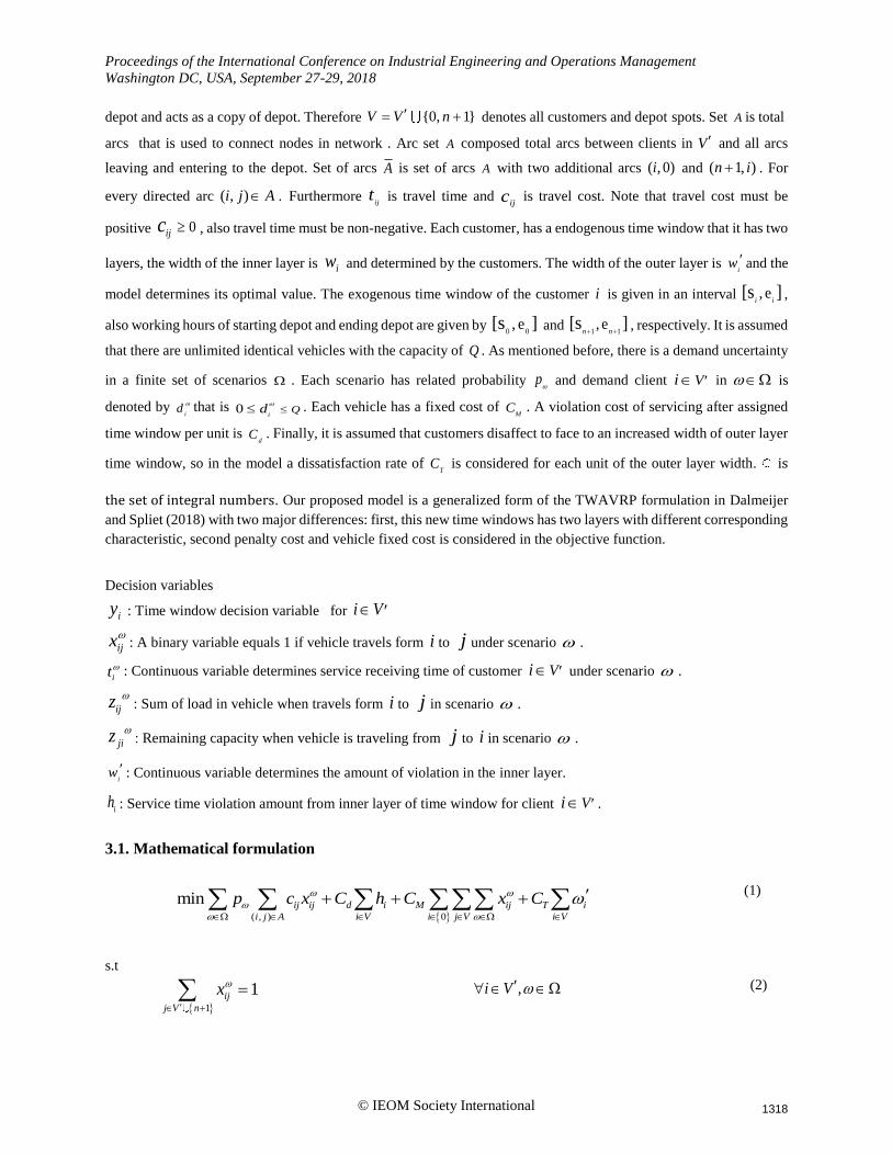
depot and acts as a copy of depot. Therefore {0, 1}V V n= + denotes all customers and depot spots. Set A is total
arcs that is used to connect nodes in network . Arc set A composed total arcs between clients in V and all arcs
leaving and entering to the depot. Set of arcs A is set of arcs A with two additional arcs ( , 0)i and ( 1, )n i+ . For
every directed arc ( , )i j A . Furthermore ij
t is travel time and ijc is travel cost. Note that travel cost must be
positive 0ijc , also travel time must be non-negative. Each customer, has a endogenous time window that it has two
layers, the width of the inner layer is iw and determined by the customers. The width of the outer layer is i
w and the
model determines its optimal value. The exogenous time window of the customer i is given in an interval , e[s ]i i
,
also working hours of starting depot and ending depot are given by 0 0, e[s ] and
1 1, e[s ]
n n+ +, respectively. It is assumed
that there are unlimited identical vehicles with the capacity of Q . As mentioned before, there is a demand uncertainty
in a finite set of scenarios . Each scenario has related probability p
and demand client Vi in is
denoted by i
d that is 0
iQd
. Each vehicle has a fixed cost of
MC . A violation cost of servicing after assigned
time window per unit is d
C . Finally, it is assumed that customers disaffect to face to an increased width of outer layer
time window, so in the model a dissatisfaction rate of T
C is considered for each unit of the outer layer width. is
the set of integral numbers. Our proposed model is a generalized form of the TWAVRP formulation in Dalmeijer
and Spliet (2018) with two major differences: first, this new time windows has two layers with different corresponding
characteristic, second penalty cost and vehicle fixed cost is considered in the objective function.
Decision variables
iy : Time window decision variable for i V
ijx: A binary variable equals 1 if vehicle travels form i to j under scenario .
it : Continuous variable determines service receiving time of customer Vi under scenario .
ijz : Sum of load in vehicle when travels form i to j in scenario .
jiz : Remaining capacity when vehicle is traveling from j to i in scenario .
iw : Continuous variable determines the amount of violation in the inner layer.
ih : Service time violation amount from inner layer of time window for client Vi .
3.1. Mathematical formulation
( , ) 0
min ij ij d i M ij T i
i j A i V i j V i V
p c x C h C x C
+ + +
(1)
s.t
1
1ij
j V n
x
+
= ,i V (2)
1318
Proceedings of the International Conference on Industrial Engineering and Operations Management
Washington DC, USA, September 27-29, 2018
© IEOM Society International
0
1ij
i V
x
= ,j V (3)
( )ij ji ij jiz z x x Q + = + ( , ) , i j,i j A (4)
( ) 2ji ij i
j V
z z d
− = ,i V (5)
0 j i
j V i V
z d
= (6)
1, 0n j j
j V j V
z x Q
+
=
(7)
0 0j j i
j V j V i V
z x Q d
= −
(8)
( )(1 )j i ij ij j i ij
t t t x s e x + + − − , ,i V j V (9)
0 0 j js t t+
,j V
(10)
, 1 1i i n nt t e
+ ++
,i V
(11)
i it y
,i V
(12)
i i i i
t y w w + +
,i V
(13)
,i i i i iy s e w w− −
i V
(14)
( )i i i ih t y w= − + ,i V
(15)
0i
h
i V
(16)
ij
x ( , ) ,i j A
(17)
1319
Proceedings of the International Conference on Industrial Engineering and Operations Management
Washington DC, USA, September 27-29, 2018
© IEOM Society International
0ij
z ( , ) ,i j A (18)
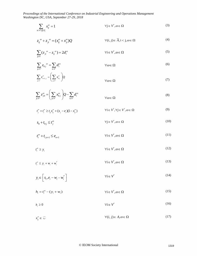
The objective function (1) minimizes the sum of fixed and variable routing and penalty costs. Penalty cost consists of
two terms including length of assigned outer layer time window and servicing time violation from the inner layer time
window. Constraints (2) and (3) ensure that each customer is visited only by one vehicle. Constraints (4) determines
used and left over capacity of a vehicle according toits capacity. Constraint (5) determines the used and left over
capacity of a vehicle according to served demand of a visited node. Constraints (6)-(8) determine the required vehicle
load and excess capacity when leaving or returning to the depot. Constraint (9) to (14) is related to both inner and
outer layers time windows for each customer. Constraint (9) is MTZ inequalities that as subtour elimination
constraints. Constraint (10) ensures that vehicle can serve a customer after leaving the depot and traveling to customer
node. Constraint (11) schedules vehicles considering the depot closing time. Constraint (12) and (13) guarantees that
each customer receive its demand after start endogenous time window and before end of it. Constraint (14) implies
that each endogenous time windows must assign within exogenous time window. Constraint (15) calculates the
amount of servicing violation from an assigned inner layer time window for each customer.Constraints (16)-(18)
define ype of variables.
4. Numerical expamples and results
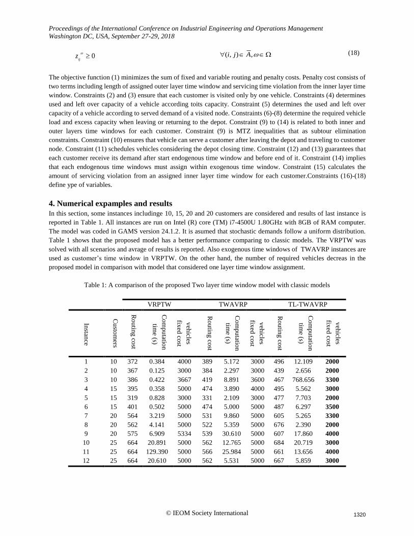
In this section, some instances includinge 10, 15, 20 and 20 customers are considered and results of last instance is
reported in Table 1. All instances are run on Intel (R) core (TM) i7-4500U 1.80GHz with 8GB of RAM computer.
The model was coded in GAMS version 24.1.2. It is asumed that stochastic demands follow a uniform distribution.
Table 1 shows that the proposed model has a better performance comparing to classic models. The VRPTW was
solved with all scenarios and avrage of results is reported. Also exogenous time windows of TWAVRP instances are
used as customer’s time window in VRPTW. On the other hand, the number of required vehicles decreas in the
proposed model in comparison with model that considered one layer time window assignment.
Table 1: A comparison of the proposed Two layer time window model with classic models
VRPTW TWAVRP TL-TWAVRP
Instan
ce
Cu
stom
ers
Ro
utin
g co
st
Co
mp
utatio
n
time (s)
veh
icles
fixed
cost
Ro
utin
g co
st
Co
mp
utatio
n
time (s)
veh
icles
fixed
cost
Ro
utin
g co
st
Co
mp
utatio
n
time (s)
veh
icles
fixed
cost
1 10 372 0.384 4000 389 5.172 3000 496 12.109 2000
2 10 367 0.125 3000 384 2.297 3000 439 2.656 2000
3 10 386 0.422 3667 419 8.891 3600 467 768.656 3300
4 15 395 0.358 5000 474 3.890 4000 495 5.562 3000
5 15 319 0.828 3000 331 2.109 3000 477 7.703 2000
6 15 401 0.502 5000 474 5.000 5000 487 6.297 3500
7 20 564 3.219 5000 531 9.860 5000 605 5.265 3300
8 20 562 4.141 5000 522 5.359 5000 676 2.390 2000
9 20 575 6.909 5334 539 30.610 5000 607 17.860 4000
10 25 664 20.891 5000 562 12.765 5000 684 20.719 3000
11 25 664 129.390 5000 566 25.984 5000 661 13.656 4000
12 25 664 20.610 5000 562 5.531 5000 667 5.859 3000
1320
Proceedings of the International Conference on Industrial Engineering and Operations Management
Washington DC, USA, September 27-29, 2018
© IEOM Society International
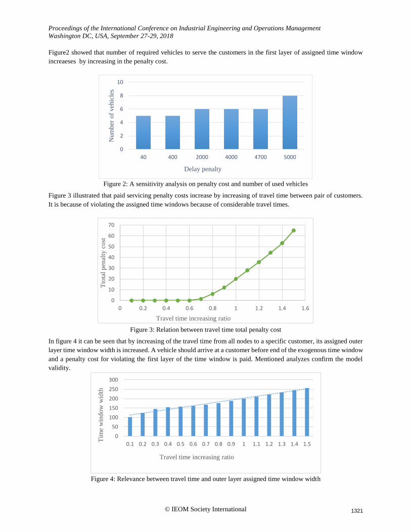
Figure2 showed that number of required vehicles to serve the customers in the first layer of assigned time window
increaeses by increasing in the penalty cost.
Figure 2: A sensitivity analysis on penalty cost and number of used vehicles
Figure 3 illustrated that paid servicing penalty costs increase by increasing of travel time between pair of customers.
It is because of violating the assigned time windows because of considerable travel times.
Figure 3: Relation between travel time total penalty cost
In figure 4 it can be seen that by increasing of the travel time from all nodes to a specific customer, its assigned outer
layer time window width is increased. A vehicle should arrive at a customer before end of the exogenous time window
and a penalty cost for violating the first layer of the time window is paid. Mentioned analyzes confirm the model
validity.
Figure 4: Relevance between travel time and outer layer assigned time window width
0
2
4
6
8
10
40 400 2000 4000 4700 5000
Num
ber
of
veh
icle
s
Delay penalty
0
10
20
30
40
50
60
70
0 0.2 0.4 0.6 0.8 1 1.2 1.4 1.6
Tto
tal
pen
alty
co
st
Travel time increasing ratio
0
50
100
150
200
250
300
0.1 0.2 0.3 0.4 0.5 0.6 0.7 0.8 0.9 1 1.1 1.2 1.3 1.4 1.5
Tim
e w
ind
ow
wid
th
Travel time increasing ratio
1321
Proceedings of the International Conference on Industrial Engineering and Operations Management
Washington DC, USA, September 27-29, 2018
© IEOM Society International
5. conclusion
In this paper, a new model of time window assignment VRP was proposed considering two-layer time window
assignment. Various sensitivity analysis confirm the proposed model validity. It was shown that more penalty cost
should be paid when we face to a problem with more travelling time. Also it was shown that widthof the outer layer
assigned time window will be increased in cases with more travel times. By the proposed model, it was concluded
that less vehicle will be needed comparing to classic models. As a future study, time window assignment may be
considered for other various types of the vehicle routing problem. Moreover, developing heuristic algorithms to solve
the largescale instances of the problem may be a s another direction for the future study.
References
Baldacci, R., Hadjiconstantinou, E. and Mingozzi, A. ‘An Exact Algorithm for the Capacitated Vehicle Routing
Problem Based on a Two-Commodity Network Flow Formulation’, Operations Research, vol. 52, no. 5, pp. 723–
738, 2004.
Dalmeijer, K. and Spliet, R. ‘A branch-and-cut algorithm for the Time Window Assignment Vehicle Routing
Problem’, Computers and Operations Research, vol 89, pp. 140-152, 2018.
Jabali, O., Leus, R., van Woensel, T., de Kok, T., ‘Self-imposed time windows in vehicle routing problems’, OR
Spectrum, vol. 37, no. 2, pp. 331–352, 2015.
Miller, C. E., Tucker, A. W. and Zemlin, R. A. ‘Integer Programming Formulation of Traveling Salesman Problems’,
Journal of the ACM, vol. 7, no. 4, pp. 326–329, 1960.
Mouthuy, S., Massen, F., Deville, Y., & Van Hentenryck, P. ‘A Multistage Very Large-Scale Neighborhood Search
for the Vehicle Routing Problem with Soft Time Windows’, Transportation Science, vol. 49, no. 2, pp. 223-238,
2015.
Neves-Moreira, F., Pereira da Silva, D., Guimarães, L., Amorim, P., & Almada-Lobo, B. ‘The time window
assignment vehicle routing problem with product dependent deliveries’, Transportation Research Part E:
Logistics and Transportation Review, vol. 116, pp. 163–183, 2018.
Oyola, J., Arntzen, H. and Woodruff, D. L. ‘The stochastic vehicle routing problem, a literature review, part I: models’,
EURO Journal on Transportation and Logistics, vol 6, no. 4, pp. 349-388, 2016.
Spliet, R., Dabia, S. and Van Woensel, T. ‘The Time Window Assignment Vehicle Routing Problem with Time-
Dependent Travel Times’, Transportation Science, no. March, pp. 1–16, 2017.
Spliet, R. and Desaulniers, G. ‘The discrete time window assignment vehicle routing problem’, European Journal of
Operational Research, vol. 244, no. 2, pp. 379–391, 2015.
Spliet, R. and Gabor, A. F. ‘The Time Window Assignment Vehicle Routing Problem’, Transportation Science, vol
49, no 4, pp. 721–731, 2014.
Taş, D., Dellaert, N., Van Woensel, T., & De Kok, T .‘Vehicle routing problem with stochastic travel times including
soft time windows and service costs’, Computers and Operations Research, vol. 40, no. 1, pp. 214–224, 2013.
Taş, D., Dellaert, N., Van Woensel, T., & De Kok, T ‘The time-dependent vehicle routing problem with soft time
windows and stochastic travel times’, Transportation Research Part C: Emerging Technologies, vol. 48, pp. 66–
83, 2014.
Taş, D., Jabali, O. and Van Woensel, T. ‘A vehicle routing problem with flexible time windows’, Computers and
Operations Research, vol. 52, no. PART A, pp. 39–54, 2014.
1322
Proceedings of the International Conference on Industrial Engineering and Operations Management
Washington DC, USA, September 27-29, 2018
© IEOM Society International
Biographies
Mahdi Jalilvand is an M.S. degree student of Industrial Engineering at Shahed University. He received his B.Sc.
degree from Bu-Ali Sina University in 2017. His research interests are facility, transportations and supply chain.
Mahdi Bashiri is a Professor of Industrial Engineering at Shahed University. He holds a B.Sc. in Industrial
Engineering from Iran University of Science and Technology, M.Sc. and Ph.D. from Tarbiat Modarres University. He
is a recipient of the 2013 young national top scientist award from the Academy of Sciences of the Islamic Republic of
Iran. He serves as the Editor-in-Chief of Journal of Quality Engineering and Production Optimization published in
Iran and the Editorial Board member of some reputable academic journals. His research interests are Facilities
Planning, Stochastic Optimization, Meta-heuristics, and Multi-response Optimization. He published about 10 books
and more than 190 papers in reputable academic journals and conferences.
1323
Recommended