A Statistical Image-Based Shape Model for Visual Hull
Reconstruction and 3D Structure Inference
by
Kristen Lorraine Grauman
Submitted to the Department of Electrical Engineering and ComputerScience
in partial fulfillment of the requirements for the degree of
Master of Science in Computer Science and Engineering
at the
MASSACHUSETTS INSTITUTE OF TECHNOLOGY
June 2003
c© Massachusetts Institute of Technology 2003. All rights reserved.
Author . . . . . . . . . . . . . . . . . . . . . . . . . . . . . . . . . . . . . . . . . . . . . . . . . . . . . . . . . . . . .Department of Electrical Engineering and Computer Science
May 9, 2003
Certified by . . . . . . . . . . . . . . . . . . . . . . . . . . . . . . . . . . . . . . . . . . . . . . . . . . . . . . . . .Trevor Darrell
Associate Professor of Electrical Engineering and Computer ScienceThesis Supervisor
Accepted by. . . . . . . . . . . . . . . . . . . . . . . . . . . . . . . . . . . . . . . . . . . . . . . . . . . . . . . . .Arthur C. Smith
Chairman, Department Committee on Graduate Students

2

A Statistical Image-Based Shape Model for Visual Hull Reconstruction
and 3D Structure Inference
by
Kristen Lorraine Grauman
Submitted to the Department of Electrical Engineering and Computer Scienceon May 9, 2003, in partial fulfillment of the
requirements for the degree ofMaster of Science in Computer Science and Engineering
Abstract
We present a statistical image-based “shape + structure” model for Bayesian visual hull re-construction and 3D structure inference. The 3D shape of a class of objects is representedby sets of contours from silhouette views simultaneously observed from multiple calibratedcameras. Bayesian reconstructions of new shapes are then estimated using a prior densityconstructed with a mixture model and probabilistic principal components analysis. Weshow how the use of a class-specific prior in a visual hull reconstruction can reduce theeffect of segmentation errors from the silhouette extraction process. The proposed methodis applied to a data set of pedestrian images, and improvements in the approximate 3Dmodels under various noise conditions are shown. We further augment the shape modelto incorporate structural features of interest; unknown structural parameters for a novel setof contours are then inferred via the Bayesian reconstruction process. Model matchingand parameter inference are done entirely in the image domain and require no explicit 3Dconstruction. Our shape model enables accurate estimation of structure despite segmen-tation errors or missing views in the input silhouettes, and works even with only a singleinput view. Using a data set of thousands of pedestrian images generated from a syntheticmodel, we can accurately infer the 3D locations of 19 joints on the body based on observedsilhouette contours from real images.
Thesis Supervisor: Trevor DarrellTitle: Associate Professor of Electrical Engineering and Computer Science
3

4

Acknowledgments
I would first like to thank my research advisor, Trevor Darrell, for the direction, enthusiasm,
and insights he shared with me throughout this work. I am also grateful for the general
support of the members in the Vision Interface Group. In particular, I would like to thank
Greg Shakhnarovich for collaborating with me on this work over the past year, and Ali
Rahimi and David Demirdjian for various helpful conversations. Thanks as well to the
anonymous CVPR reviewers for their feedback on a paper we wrote earlier dealing with
part of this research.
I appreciate the support of the Department of Energy, who has funded me with the
Computational Science Graduate Fellowship for the past two years.
I am especially grateful to Mark Stephenson for being a constant source of support, wis-
dom, and encouragement. Finally, I extend great gratitude to Karen and Robert Grauman,
my parents, whose inspiration and love have guided me always.
5

6
Contents
1 Introduction 11
1.1 Motivation . . . . . . . . . . . . . . . . . . . . . . . . . . . . . . . . . . . 11
1.1.1 Visual Hull Reconstruction . . . . . . . . . . . . . . . . . . . . . . 11
1.1.2 3D Structure Estimation . . . . . . . . . . . . . . . . . . . . . . . 12
1.2 Proposed Shape and Structure Model . . . . . . . . . . . . . . . . . . . . . 15
1.2.1 Shape Component of the Model . . . . . . . . . . . . . . . . . . . 15
1.2.2 Structure Component of the Model . . . . . . . . . . . . . . . . . . 16
1.2.3 Learning the Model . . . . . . . . . . . . . . . . . . . . . . . . . . 16
1.3 Roadmap . . . . . . . . . . . . . . . . . . . . . . . . . . . . . . . . . . . 17
2 Related Work 19
2.1 Computing a Visual Hull . . . . . . . . . . . . . . . . . . . . . . . . . . . 19
2.2 Contours and Low-Dimensional Manifolds . . . . . . . . . . . . . . . . . 20
2.3 Estimating 3D Structure . . . . . . . . . . . . . . . . . . . . . . . . . . . 21
2.3.1 Model Matching Directly from Observations . . . . . . . . . . . . 22
2.4 Contributions . . . . . . . . . . . . . . . . . . . . . . . . . . . . . . . . . 22
3 Bayesian Multi-View Shape Reconstruction 25
3.1 Multi-View Observation Manifolds . . . . . . . . . . . . . . . . . . . . . . 26
3.2 Contour-Based Shape Density Models . . . . . . . . . . . . . . . . . . . . 27
3.2.1 Prior Density Model . . . . . . . . . . . . . . . . . . . . . . . . . 27
3.2.2 Observation Likelihood Density Model . . . . . . . . . . . . . . . 28
3.3 Bayesian Reconstruction . . . . . . . . . . . . . . . . . . . . . . . . . . . 29
7

3.4 Robust Reconstruction Using Random Sample Consensus . . . . . . . . . . 30
4 Visual Hull Reconstruction from Pedestrian Images 33
4.1 Description of the Data Set . . . . . . . . . . . . . . . . . . . . . . . . . . 33
4.2 Representation . . . . . . . . . . . . . . . . . . . . . . . . . . . . . . . . 34
4.3 Expected Variation of the Data . . . . . . . . . . . . . . . . . . . . . . . . 36
4.4 Results . . . . . . . . . . . . . . . . . . . . . . . . . . . . . . . . . . . . . 37
5 Inferring 3D Structure 47
5.1 Extending the Shape Model . . . . . . . . . . . . . . . . . . . . . . . . . . 47
5.2 Advantages of the Model . . . . . . . . . . . . . . . . . . . . . . . . . . . 48
6 Inferring 3D Structure in Pedestrian Images 51
6.1 Advantages of a Synthetic Training Set . . . . . . . . . . . . . . . . . . . . 51
6.2 Description of the Training Set . . . . . . . . . . . . . . . . . . . . . . . . 52
6.3 Representation for the Extended Shape Model . . . . . . . . . . . . . . . . 53
6.4 Description of the Synthetic Test Set . . . . . . . . . . . . . . . . . . . . . 53
6.5 Results . . . . . . . . . . . . . . . . . . . . . . . . . . . . . . . . . . . . . 54
6.5.1 Error Measures . . . . . . . . . . . . . . . . . . . . . . . . . . . . 54
6.5.2 Training on One View Versus Training on Multiple Views . . . . . 55
6.5.3 Testing with Missing Views . . . . . . . . . . . . . . . . . . . . . 55
6.5.4 Testing on Real Data . . . . . . . . . . . . . . . . . . . . . . . . . 59
6.5.5 Results Summary . . . . . . . . . . . . . . . . . . . . . . . . . . . 60
7 Conclusions and Future Work 65
A Random Sample Consensus (RANSAC) for Multi-View Contour Reconstruc-
tion 67
8

List of Figures
1-1 The limitations of deterministic image-based visual hull construction. . . . 13
1-2 The 3D structure estimation problem. . . . . . . . . . . . . . . . . . . . . 14
2-1 Schematic illustration of the geometry of visual hull construction as inter-
section of visual cones. . . . . . . . . . . . . . . . . . . . . . . . . . . . . 20
3-1 Illustration of prior and observed densities. . . . . . . . . . . . . . . . . . 31
4-1 An example of visual hull reconstruction data. . . . . . . . . . . . . . . . . 34
4-2 Diagram of data flow: using the probabilistic shape model for visual hull
reconstruction. . . . . . . . . . . . . . . . . . . . . . . . . . . . . . . . . 35
4-3 Primary modes of variation for the multi-view contours. . . . . . . . . . . . 36
4-4 Comparison of segmentation error distributions for raw images and their
Bayesian reconstructions. . . . . . . . . . . . . . . . . . . . . . . . . . . . 38
4-5 Example of visual hull segmentation improvement with Bayesian recon-
struction. . . . . . . . . . . . . . . . . . . . . . . . . . . . . . . . . . . . 39
4-6 Example of visual hull segmentation improvement with Bayesian recon-
struction. . . . . . . . . . . . . . . . . . . . . . . . . . . . . . . . . . . . 40
4-7 Example of visual hull segmentation improvement with Bayesian recon-
struction. . . . . . . . . . . . . . . . . . . . . . . . . . . . . . . . . . . . 41
4-8 Example of visual hull segmentation improvement with Bayesian recon-
struction. . . . . . . . . . . . . . . . . . . . . . . . . . . . . . . . . . . . 42
4-9 Example of visual hull segmentation improvement with Bayesian recon-
struction. . . . . . . . . . . . . . . . . . . . . . . . . . . . . . . . . . . . 43
9

4-10 Example of visual hull segmentation improvement with Bayesian recon-
struction. . . . . . . . . . . . . . . . . . . . . . . . . . . . . . . . . . . . 44
4-11 Example of visual hull segmentation improvement with Bayesian recon-
struction. . . . . . . . . . . . . . . . . . . . . . . . . . . . . . . . . . . . 45
4-12 Example of visual hull segmentation improvement with Bayesian recon-
struction. . . . . . . . . . . . . . . . . . . . . . . . . . . . . . . . . . . . 46
5-1 Diagram of data flow: using the probabilistic shape model for 3D structure
inference. . . . . . . . . . . . . . . . . . . . . . . . . . . . . . . . . . . . 48
6-1 An example of synthetically generated training data. . . . . . . . . . . . . 52
6-2 Noisy synthetic test silhouettes. . . . . . . . . . . . . . . . . . . . . . . . . 54
6-3 Training on single view vs. training on multiple views. . . . . . . . . . . . 56
6-4 Inferring structure from only a single view. . . . . . . . . . . . . . . . . . 57
6-5 Inferring structure with one missing view. . . . . . . . . . . . . . . . . . . 58
6-6 Summary of missing view results. . . . . . . . . . . . . . . . . . . . . . . 59
6-7 Inferring structure on real data. . . . . . . . . . . . . . . . . . . . . . . . . 61
6-8 Inferring structure on real data with two missing views. . . . . . . . . . . . 62
6-9 Inferring structure on real data with two missing views. . . . . . . . . . . . 63
6-10 Inferring structure on real data from only a single view. . . . . . . . . . . . 64
A-1 RANSAC variant for robust reconstruction of multi-view contours. . . . . . 68
10

Chapter 1
Introduction
Implicit representations of 3D shape can be formed using models of observed contours and
feature locations in multiple views. With sufficient training data of objects of a known
class, a statistical multi-view appearance model can represent the most likely shapes in that
class. Such a model can be used to reduce noise in observed images, or to fill in missing
data. In this work we present a contour-based probabilistic shape model and use it to give
both a probabilistic version of image-based visual hull reconstruction and an image-based
method for inferring 3D structure parameters.
1.1 Motivation
1.1.1 Visual Hull Reconstruction
Reconstruction of 3D shape using the intersection of object silhouettes from multiple views
can yield a surprisingly accurate shape model, if accurate contour segmentation is available.
Algorithms for computing the visual hull of an object have been developed based on the
explicit geometric intersection of generalized cones [17]. More recently methods that per-
form resampling operations purely in the image planes have been developed [21], as well
as approaches using weakly calibrated or uncalibrated views [18, 32].
Visual hull algorithms have the advantage that they can be very fast to compute and
re-render, and they are also much less expensive in terms of storage requirements than
11

volumetric approaches such as voxel carving or coloring [16, 26, 28]. With visual hulls
view-dependent re-texturing can be used, provided there is accurate estimation of the alpha
mask for each source view [22]. When using these techniques a relatively small number of
views (4-8) is often sufficient to recover models that appear compelling and are useful for
creating real-time virtual models of objects and people in the real world, or for rendering
new images for view-independent recognition using existing view-dependent recognition
algorithms [27].
Unfortunately most algorithms for computing visual hulls are deterministic in nature,
and they do not model any uncertainty that may be present in the observed contour shape
in each view. They can also be quite sensitive to segmentation errors: since the visual hull
is defined as the 3D shape which is the intersection of the observed silhouettes, a small
segmentation error in even a single view can have a dramatic effect on the resulting 3D
model (see Figure 1-1).
Traditional visual hull algorithms (e.g., [21]) have the advantage that they are general
– they can reconstruct any 3D shape which can be projected to a set of silhouettes from
calibrated views. While this is a strength, it is also a weakness of the approach. Even though
parts of many objects cannot be accurately represented by a visual hull (e.g, concavities),
the set of objects that can be represented is very large, and often larger than the set of objects
that will be physically realizable. Structures in the world often exhibit local smoothness,
which is not accounted for in deterministic visual hull algorithms1. Additionally, many
applications may have prior knowledge about the class of objects to be reconstructed, e.g.
pedestrian images as in the gait recognition system of [27]. Existing algorithms cannot
exploit this knowledge when performing reconstruction or re-rendering.
1.1.2 3D Structure Estimation
Estimating model shape or structure parameters from one or more input views is an impor-
tant computer vision problem that has received considerable attention in recent years [11].
1In practice many implementations use preprocessing stages with morphological filters to smooth seg-mentation masks before geometric intersection, but this may not reflect the statistics of the world and couldlead to a shape bias.
12

(a) Camera input
(b) Traditional visual hull construction
(c) Proposed probabilistic visual hull construction
Figure 1-1: The limitations of deterministic image-based visual hull construction. Segmen-tation errors in the silhouettes cause dramatic effects on the approximate 3D model (b). Aprobabilistic reconstruction can reduce these adverse effects (c).
13

(a) Input
0 0.1 0.2 0.3 0.4
0
0.1
0.2
0.3
0.4
0.5
0.6
0 0.10.2
lankle
ltoe
lelbow
lknee
lwrist lt
lshoulder
rt
n
rs
thead
bhead
relbow
rankle
rwrist
rknee
rtoe
(b) Desired output
Figure 1-2: The 3D structure estimation problem: given one or more views of an object,infer the 3D locations of structural points of interest. For instance, given some number ofviews of a human body, estimate the 3D locations of specific body parts.
The idea is to estimate 3D locations or angles between parts of an articulated object using
some number of 2D images of that object. If the class of objects is people, for instance,
the goal may be to obtain estimates of the 3D locations of different body parts in order
to describe the body’s pose (see Figure 1-2). These estimates can then be passed on to a
higher-level application that performs a task such as gesture recognition, pose estimation,
gait recognition, or character creation in a virtual environment. There is a large body of
work in the computer vision and human-computer interfaces communities devoted to these
topics alone.
Although we do not consider temporal constraints in this work, many techniques for
human body tracking require the initial pose to be given for the first video frame either
through a hand initialization step or by having the subject stand in a canonical pose. Thus
another application of our method for inferring structure is to automate that initialization
process and make it more flexible.
Additionally, for any object class where it is possible to establish feature correspon-
dences between instances of the class, estimating the 3D locations of key points on the ob-
ject would allow this correspondence to be established automatically. For instance, when
matching a novel set of images to a 3D morphable model, correspondences must be estab-
lished between multiple key points on the object and the same key points on the model. A
14
means of estimating the designated locations based on the input images would allow the
model to be matched automatically.
Classic techniques for structure estimation attempt to detect and align 3D model in-
stances within the image views, but high-dimensional models or models without well-
defined features may make this type of search computationally prohibitive. It is an expen-
sive task to iteratively align a 3D model so that its 2D projections fit the observed image
features, and the difficulty of such model-based techniques is compounded if the class of
objects lacks features that are consistently identifiable in the input image views.
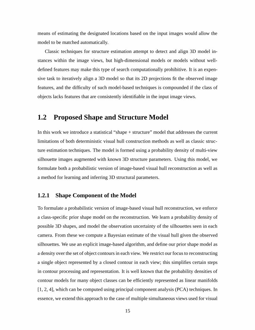
1.2 Proposed Shape and Structure Model
In this work we introduce a statistical “shape + structure” model that addresses the current
limitations of both deterministic visual hull construction methods as well as classic struc-
ture estimation techniques. The model is formed using a probability density of multi-view
silhouette images augmented with known 3D structure parameters. Using this model, we
formulate both a probabilistic version of image-based visual hull reconstruction as well as
a method for learning and inferring 3D structural parameters.
1.2.1 Shape Component of the Model
To formulate a probabilistic version of image-based visual hull reconstruction, we enforce
a class-specific prior shape model on the reconstruction. We learn a probability density of
possible 3D shapes, and model the observation uncertainty of the silhouettes seen in each
camera. From these we compute a Bayesian estimate of the visual hull given the observed
silhouettes. We use an explicit image-based algorithm, and define our prior shape model as
a density over the set of object contours in each view. We restrict our focus to reconstructing
a single object represented by a closed contour in each view; this simplifies certain steps
in contour processing and representation. It is well known that the probability densities of
contour models for many object classes can be efficiently represented as linear manifolds
[1, 2, 4], which can be computed using principal component analysis (PCA) techniques. In
essence, we extend this approach to the case of multiple simultaneous views used for visual
15

hull reconstruction.
1.2.2 Structure Component of the Model
Rather than fit explicit 3D models to input images, we perform parameter inference using
our image-based shape model, which can be matched directly to observed features. The
shape model composed of multi-view contours is extended to include the 3D locations of
key points on the object. We then estimate the missing 3D structure parameters for a novel
set of contours by matching them to the statistical model and inferring the 3D parameters
from the matched model.
Utilizing the same Bayesian framework described above, a reconstruction of an ob-
served object yields the multi-view contours and their 3D structure parameters simultane-
ously. To our knowledge, this is the first work to formulate an image-based multi-view
statistical shape model for the inference of 3D structure.
In our experiments, we demonstrate how our shape + structure model enables accurate
estimation of structure parameters despite large segmentation errors or even missing views
in the input silhouettes. Since parameter inference with our model succeeds even with
missing views, it is possible to match the model with fewer views than it has been trained
on. We also show how configurations that are typically ambiguous in single views are
handled well by our multi-view model.
1.2.3 Learning the Model
In this work we also show how the image-based model can be learned from a known 3D
shape model. Using a computer graphics model of articulated human bodies, we render
a database of views augmented with the known 3D feature locations (and optionally joint
angles, etc.) From this we learn a joint shape and structure model prior, which can be used
to find the instance of the model class that is closest to a new input image. One advantage of
a synthetic training set is that labeled real data is not required; the synthetic model includes
3D structure parameter labels for each example.
For applications where it is desirable to have reconstructed silhouettes that closely pre-
16

serve the same underlying contours and idiosyncrasies of the input data, e.g., for visual hull
reconstructions used in recognition applications, the shape model may be trained on a set
of relatively cleanly segmented examples of real data.
1.3 Roadmap
In the following chapter we review related previous work on visual hulls, probabilistic
contour models, and image-based statistical shape models that can be directly matched
to observed shape contours. In Chapter 3 we formulate the Bayesian multi-view shape
reconstruction method which underlies our model. In Chapter 4 we present results from
our experiments applying the proposed visual hull reconstruction method to a data set of
pedestrian images. Then in Chapter 5 we formulate the extended shape model which allows
the inference of 3D structure. In Chapter 6 we describe the means of learning such a model
from synthetic data, and we present results from our experiments applying the proposed
structure inference method to the data set of pedestrian images in order to locate 19 joints
of the body in 3D. Finally, we conclude in Chapter 7 and suggest several avenues for future
work.
17

18

Chapter 2
Related Work
In the this chapter we review related previous work on visual hulls, probabilistic contour
models, and image-based statistical shape models that can be directly matched to observed
shape contours.
2.1 Computing a Visual Hull
A visual hull (VH) is defined by a set of camera locations, the cameras’ internal calibration
parameters, and silhouettes from each view. Most generally, it is the maximal volume
whose projections onto multiple image planes result in the set of observed silhouettes of an
object. The VH is known to include the object, and to be included in the object’s convex
hull. In practice, the VH is usually computed with respect to a finite, often small, number
of silhouettes. (See Figure 2-1.) One efficient technique for generating the VH computes
the intersection of the viewing ray from each designated viewpoint with each pixel in that
viewpoint’s image [21]. A variant of this algorithm approximates the surface of the VH
with a polygonal mesh [20]. See [17, 20, 21] for the details of these methods.
While we restrict our attention to visual hulls from calibrated cameras, recent work has
shown that visual hulls can be computed from weakly calibrated or uncalibrated views [18,
32]. Detailed models can be constructed from visual hulls with view-dependent reflectance
or texture and accurate modeling of opacity [22].
A traditional application of visual hulls is the creation of models for populating virtual
19

Figure 2-1: Schematic illustration of the geometry of visual hull construction as intersec-tion of visual cones.
worlds, either for detailed models computed offline using many views (perhaps acquired
using a single camera and turntable), or for online acquisition of fast and approximate
models for real-time interaction. Visual hulls can also be used in recognition applications.
Recognition can be performed directly on visible 3D structures from the visual hull (espe-
cially appropriate for the case of orthogonal virtual views), or the visual hull can be used in
conjunction with traditional 2D recognition algorithms. In [27] a system was demonstrated
that rendered virtual views of a moving pedestrian for integrated face and gait recognition
using existing 2D recognition algorithms.
2.2 Contours and Low-Dimensional Manifolds
The authors of [1] developed a single-view model of pedestrian contours, and showed how a
linear subspace model formed from principal components analysis (PCA) could represent
and track a wide range of motion [2]. A model appropriate for feature point locations
20

sampled from a contour is also given in [2]. This single-view approach can be extended to
3D by considering multiple simultaneous views of features. The Active Shape Model of
[5] was successfully applied to model facial variation.
The use of linear manifolds estimated by PCA to represent an object class, and more
generally an appearance model, has been developed by several authors [4, 14, 30]. A
probabilistic interpretation of PCA-based manifolds has been introduced in [12, 31] as
well as in [23], where it was applied directly to face images. Snakes [15] and Condensation
(particle filtering) [13] have also been used to exploit prior knowledge while tracking single
contours. We rely on the mixture of probabilistic principal components analyzers (PPCA)
formulation of [29] to model the prior density as a mixture of Gaussians.
2.3 Estimating 3D Structure
There has been considerable work on the general problem of estimating structure param-
eters from images, particularly for the estimation of human body part configurations or
“pose”. See [11] for a survey.
As described in [11], approaches to pose estimation may be generally categorized into
three groups: 2D approaches that do not use explicit shape models, 2D approaches that
do use explicit shape models, and 3D approaches that use a 3D model for estimating the
positions of articulated structures. A 2D approach without an explicit shape model will
apply either a statistical model or simple heuristic to directly observable features in the
image. In contrast, a 2D explicit shape model makes use of a priori knowledge of how
the object appears in 2D and attempts to segment and label specific parts of the object in
an input image. Finally, 3D approaches attempt to fit a 3D model to some number of 2D
images, often utilizing a priori knowledge about the kinematic and shape properties of the
object class, and typically requiring a hand-initialized reference frame. In practice, a priori
kinematic and shape constraints may be difficult to describe efficiently and thoroughly, and
they require significant knowledge about the structure and movement patterns of the given
object class.
Our work on 3D structure inference falls into the first category: we infer structure (or
21

pose) using observable features in multi-view images without constructing an explicit shape
model. We do not require that any class-specific a priori kinematic or shape constraints
be explicitly specified; the only prior information utilized is learned directly from easily
extracted features in the training set images.
Note that in this work we are not considering any temporal constraints, so we are inter-
ested in the related work in pose estimation to the extent which it analyzes a single frame
at a time.
2.3.1 Model Matching Directly from Observations
We consider image-based statisical shape models that can be directly matched to observed
shape contours. Models which capture the 2D distribution of feature point locations have
been shown to be able to describe a wide range of flexible shapes, and they can be directly
matched to input images [5]. A drawback of such single-view models is that features need
to be present, i.e., not occluded, at all times. Shape models in several views can be sepa-
rately estimated to match object appearance [6]; this approach was able to learn a mapping
between the low-dimensional shape parameters in each view. Typically these shape models
require a good initialization in order for the model matching method to converge properly.
The idea of augmenting a PCA-based appearance model with structure parameters and
using projection-based reconstruction to fill in the missing values of those parameters for
new images was first proposed in [7]. A method that used a mixture of PCA approach
to learn a model of single contour shape augmented with 3D structure parameters was
presented in [25]. They were able to estimate 3D hand and arm location just from a single
silhouette. This system was also able to model contours observed in two simultaneous
views, but separate models were formed for each so no implicit model of 3D shape was
formed.
2.4 Contributions
While regularization or Bayesian maximum a posteriori (MAP) estimation of single-view
contours has received considerable attention, relatively little attention has been given to
22

multi-view data from several cameras simultaneously observing an object. With multi-view
data, a probabilistic model and MAP estimate can be computed on implicit 3D structures.
In this work we apply a PPCA-based probability model to form Bayesian estimates of
multi-view contours used for visual hull reconstruction and 3D structure inference.
The strength of our approach lies in our use of a probabilistic multi-view shape model
which restricts the object shape and its possible structural configurations to those that are
most probable given the object class and the current observation. Even when given poorly
segmented binary images of the object, the statistical model can infer more accurate sil-
houette segmentations and appropriate structure parameters. Moreover, all computation is
done within the image domain, and no model matching or search in 3D space is required.
Our model may be learned from synthetic training data when a computer graphics 3D
shape model is available. As we will discuss in Chapter 6, using a synthetic training set is a
practical way to generate a large volume of data, it guarantees precise ground truth labels,
and it eliminates some dangers of segmentation bias that real training data may possess.
The experiments we present in this work show good results on a data set of pedestrian
images. However, the shape model and reconstruction method we propose have no inherent
specification for this particular object class; the methods we present are intended for use
on any class of objects for which the global shape of different instances of the object class
is roughly similar.
23

24

Chapter 3
Bayesian Multi-View Shape
Reconstruction
In this work, we derive a multi-view contour density model for 3D visual hull reconstruc-
tion and 3D structure inference. We represent the silhouette shapes as sampled points on
closed contours, with the shape vectors for each view concatenated to form a single vector
in the input space. Our algorithm can be extended to a fixed number of distinguishable
objects by concatenating their shape vectors, and to disconnected shapes more general than
those representable by a closed contour if we adopt the level-set approach put forth in [19].
As discussed in the previous chapter, many authors have shown that a probabilistic
contour model using PCA-based density models can be useful for tracking and recognition.
An appealingly simple technique is to approximate a shape space with a linear manifold
[5]. In practice, it is often difficult to represent complex, deformable structures using a
single linear manifold.
Following [4, 29], we construct a density model using a mixture of Gaussians PPCA
model that locally models clusters of data in the input space with probabilistic linear man-
ifolds. We model the uncertainty of a novel observation and obtain a MAP estimate for the
low-dimensional coordinates of the input vector, effectively using the class-specific shape
prior to restrict the range of probable reconstructions.
In the following section we see that if the 3D object can be described by linear bases,
then an image-based visual hull representation of the approximate 3D shape of that object
25
should also lie on a linear manifold, at least for the case of affine cameras.
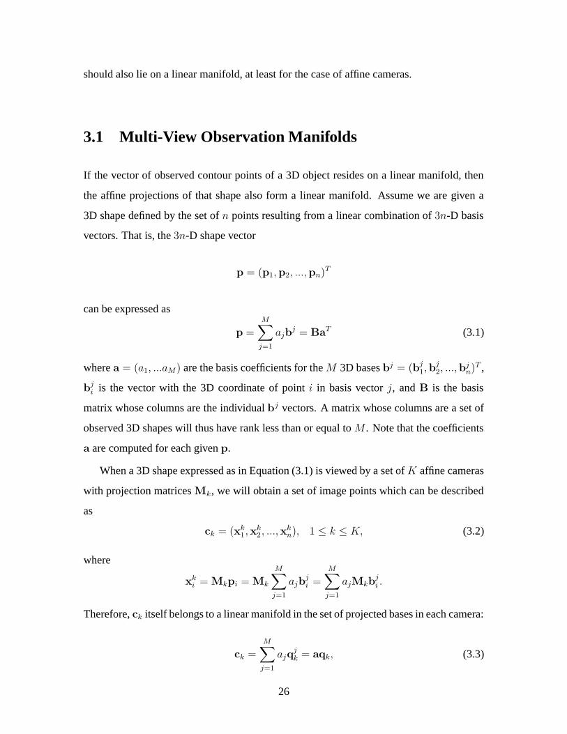
3.1 Multi-View Observation Manifolds
If the vector of observed contour points of a 3D object resides on a linear manifold, then
the affine projections of that shape also form a linear manifold. Assume we are given a
3D shape defined by the set of n points resulting from a linear combination of 3n-D basis
vectors. That is, the 3n-D shape vector
p = (p1,p2, ...,pn)T
can be expressed as
p =
M∑
j=1
ajbj = BaT (3.1)
where a = (a1, ...aM) are the basis coefficients for the M 3D bases bj = (bj1,b
j2, ...,b
jn)T ,
bji is the vector with the 3D coordinate of point i in basis vector j, and B is the basis
matrix whose columns are the individual bj vectors. A matrix whose columns are a set of
observed 3D shapes will thus have rank less than or equal to M . Note that the coefficients
a are computed for each given p.
When a 3D shape expressed as in Equation (3.1) is viewed by a set of K affine cameras
with projection matrices Mk, we will obtain a set of image points which can be described
as
ck = (xk1,x
k2, ...,x
kn), 1 ≤ k ≤ K, (3.2)
where
xki = Mkpi = Mk
M∑
j=1
ajbji =
M∑
j=1
ajMkbji .
Therefore, ck itself belongs to a linear manifold in the set of projected bases in each camera:
ck =
M∑
j=1
ajqjk = aqk, (3.3)
26

where qjk is the projected image of 3D basis bj in camera k:
qjk = (Mkb
j1,Mkb
j2, ...Mkb
jn)T .
A matrix whose columns are a set of observed 2D points will thus have rank less than
or equal to M . For the construction of Equations (3.1) - (3.3), we assume an ideal dense
sampling of points on the surface. The equations hold for the projection of all points on that
surface, as well as for any subset of the points. If some points are occluded in the imaging
process, or we only view a subset of the points (e.g., those on the occluding contour of
the object in each camera view), the resulting subset of points can still be expressed as in
Equation (3.3) with the appropriate rows deleted. The rank constraint will still hold in this
reduced matrix.
It is clear from the above discussion that if the observed points of the underlying 3D
shape lie on an M-dimensional linear manifold, then the concatenation of the observed
points in each of the K views
on = (c1, c2, ..., cK)T
can also be expressed as a linear combination of similarly concatenated projected basis
views qjk. Thus an observation matrix constructed from multiple instances of on will still
be at most rank M .
3.2 Contour-Based Shape Density Models
3.2.1 Prior Density Model
We should thus expect that when the variation in a set of 3D objects is well-approximated
by a linear manifold, their multi-view projection will also lie on a linear manifold of equal
or lower dimension. When this is the case, we can approximate the density using PPCA
with a single Gaussian. For more general object classes, object variation may only locally
lie on a linear manifold; in these cases a mixture of manifolds can be used to represent the
27

shape model [4, 29].
We construct a density model using a mixture of Gaussians PPCA model that locally
models clusters of data in the input space with probabilistic linear manifolds. An obser-
vation is the concatenated vector of sampled contour points from multiple views. Each
mixture component is a probability distribution over the observation space for the true
underlying contours in the multi-view image. Parameters for the C components are de-
termined from the set of observed data vectors on, 1 ≤ n ≤ N , using an Expectation
Maximization (EM) algorithm to maximize a single likelihood function
L =
N∑
n=1
log
C∑
i=1
πip(on|i) (3.4)
where p(o|i) is a single component of the mixture of Gaussians PPCA model, and πi is
the ith component’s mixing proportion. A separate mean vector µi, principal axes Wi,
and noise variance σi are associated with each of the C components. As this likelihood is
maximized, both the appropriate partitioning of the data and the respective principal axes
are determined. We used the Netlab [24] implementation of [29] to estimate the PPCA
mixture model.
The mixture of probabilistic linear subspaces constitutes the prior density for the ob-
ject shape. All of the images in the training set are projected into each of the subspaces
associated with the mixture components, and the resulting means µti and covariances Σt
i of
those projected coefficients are retained. The prior density is thus defined as a mixture of
Gaussians, P (P) =∑C
i=1 πiN(µti,Σ
ti).
3.2.2 Observation Likelihood Density Model
The projection y of observation on is defined as a weighted sum of the projections into
each mixture component’s subspace,
y =
C∑
i=1
p(i|on)(WiT (on − µi)), (3.5)
28

where p(i|on) is the posterior probability of component i given the observation. To account
for camera noise or jitter, we model the observation likelihood as a Gaussian distribution
on the manifold with mean µo = y and covariance Σo: P (o|P) = N(µo,Σo), where P is
the shape.
To estimate the parameter Σo from the data, we obtain manual segmentations for some
set of novel images and calculate the covariance of the differences between their projections
Ytrue into the subspaces and the projections Yobs of the contours obtained for those same
images by an automatic background subtraction algorithm,
D = Ytrue − Yobs,
Σi,jo = E[(di − E[di])(dj − E[dj ])].
(3.6)
3.3 Bayesian Reconstruction
Applying Bayes rule, we see that
P (P = y | o) ∝ P (o | P = y) P (P = y).
Thus the posterior density is the mixture of Gaussians that results from multiplying the
Gaussian likelihood and the mixture of Gaussians prior:
P (P = y | o) ∝C∑
i=1
πiN(µpi ,Σ
pi ). (3.7)
By distributing the single Gaussian across the mixture components of the prior, we see
that the components of the posterior have means and covariances
Σpi = (Σt
i−1
+ Σ−1o )−1,
µpi = Σp
i Σti−1
µti + Σp
i Σ−1o y.
(3.8)
The modes of this function are then found using a fixed-point iteration algorithm as
described in [3]. The maximum of these modes, x∗, corresponds to the MAP estimate, i.e.,
the most likely lower-dimensional coordinates in the subspace for our observation given the
29

prior1. It is backprojected into the multi-view image domain to generate the reconstructed
silhouettes S. The backprojection is a weighted sum of the MAP estimate multiplied by
the PCA bases from each mixture component of the prior:
S =
C∑
i=1
p(i|x∗)(Wi(WiTWi)
−1x∗ + µi). (3.9)
By characterizing which projections into the subspace are most likely, we restrict the
range of reconstructions to be more like that present in the training set (see Figure 3-1). Our
regularization parameter is Σo, the covariance of the density representing the observation’s
PCA coefficients. It controls the extent to which the training set’s coefficients guide our
estimate.
3.4 Robust Reconstruction Using Random Sample Con-
sensus
If a gross segmentation error causes some portion of the contour points to appear a great
distance from the true underlying contour, then the Bayesian reconstructed contour will
be heavily biased by those outlier points. Thus, to further improve the silhouette recon-
struction process, a robust contour fitting scheme may be used as a pre-processing stage
to the framework described above. We use a variant of the Random Sample Consensus
(RANSAC) algorithm in order to iteratively search for the “inlier” points from the raw in-
put contour [9]. Only these points are used to perform the Bayesian reconstruction. See
Appendix A for details on this algorithm.
1Note that for a single Gaussian PPCA model with prior N(µt,Σt), the MAP estimate is simply
x∗ =(Σ−1
t + Σ−1o
)−1 (Σ−1
t µt + Σ−1o y
).
30

training example
−5 0 5−4
−3
−2
−1
0
1
2
3
projection coefficients, 8th dim
proj
ectio
n co
effic
ient
s, 9
th d
im
test example, outlier shape
test example, outlier shape
test example, outlier shape
Figure 3-1: Illustration of prior and observed densities. Center plot shows two projectioncoefficients in the subspace for training vectors (red dots) and test vectors (green stars),all from real data. The distribution of cleanly segmented silhouettes (such as the multi-view image in top left) is representative of the prior shape density learned from the trainingset. The test points are poorly segmented silhouettes which represent novel observations.Shown in bottom left and on right are some test points lying far from the center of the priordensity. Due to large segmentation errors, they are unlikely samples according to the priorshape model. MAP estimation reconstructs such contours as shapes closer to the prior.Eighth and ninth dimensions are shown here; other dimensions are similar.
31

32

Chapter 4
Visual Hull Reconstruction from
Pedestrian Images
In this chapter we describe how our shape model is used to do probabilistic image-based
visual hull reconstruction, and we report results from our experiments with a data set of
pedestrian images.
4.1 Description of the Data Set
For the following experiments, we used an imaging model consisting of four monocular
views from cameras located at approximately the same height about 45 degrees apart. The
working space of the system is defined as the intersection of their fields of view. Im-
ages of subjects walking through the space at various directions are captured, and a simple
statistical color background model is employed to extract the silhouette foreground from
each viewpoint. The use of a basic background subtraction method results in rough seg-
mentation; body parts are frequently truncated in the silhouettes where the background is
not highly textured, or else parts are inaccurately distended due to common segmentation
problems from shadows or other effects. (See Figure 4-1 for example images from the
experimental setup.)
The goal is to improve segmentation in the multi-view frames by reconstructing prob-
lematic test silhouettes based on MAP estimates of their projections into the mixture of
33
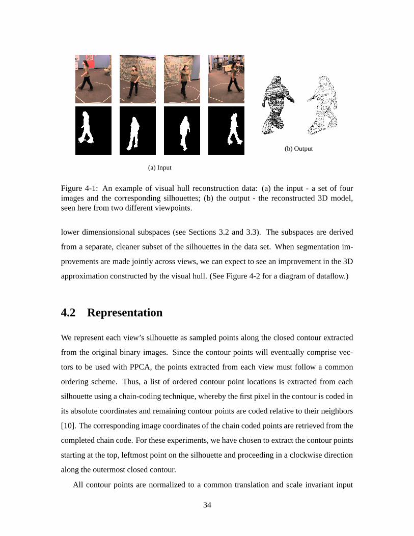
(a) Input
(b) Output
Figure 4-1: An example of visual hull reconstruction data: (a) the input - a set of fourimages and the corresponding silhouettes; (b) the output - the reconstructed 3D model,seen here from two different viewpoints.
lower dimensionsional subspaces (see Sections 3.2 and 3.3). The subspaces are derived
from a separate, cleaner subset of the silhouettes in the data set. When segmentation im-
provements are made jointly across views, we can expect to see an improvement in the 3D
approximation constructed by the visual hull. (See Figure 4-2 for a diagram of dataflow.)
4.2 Representation
We represent each view’s silhouette as sampled points along the closed contour extracted
from the original binary images. Since the contour points will eventually comprise vec-
tors to be used with PPCA, the points extracted from each view must follow a common
ordering scheme. Thus, a list of ordered contour point locations is extracted from each
silhouette using a chain-coding technique, whereby the first pixel in the contour is coded in
its absolute coordinates and remaining contour points are coded relative to their neighbors
[10]. The corresponding image coordinates of the chain coded points are retrieved from the
completed chain code. For these experiments, we have chosen to extract the contour points
starting at the top, leftmost point on the silhouette and proceeding in a clockwise direction
along the outermost closed contour.
All contour points are normalized to a common translation and scale invariant input
34
Sampled, normalizedcontour points
Silhouettes
Multi-viewtextured images
subtractionBackground
Reconstructedsilhouettes
PPCA models
Real, well-segmentedtraining images
Approximate3D model
Image-basedvisual hull
construction
Sampled, normalizedcontour points
EM
Reconstruction viaprobabilistic shape model
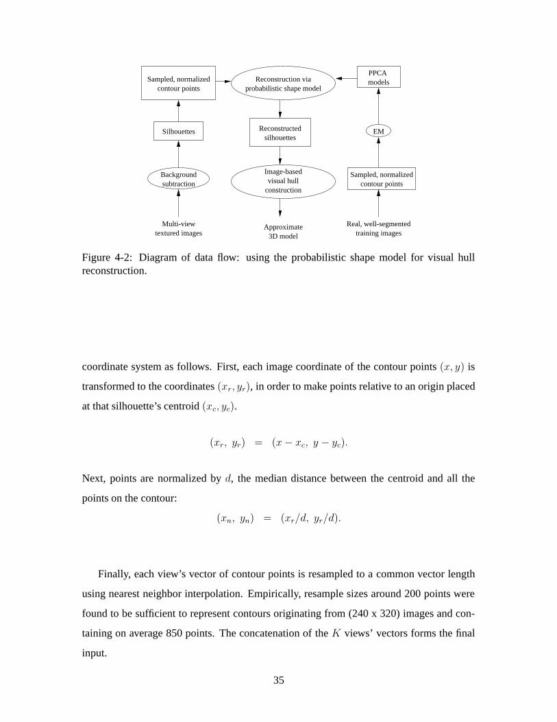
Figure 4-2: Diagram of data flow: using the probabilistic shape model for visual hullreconstruction.
coordinate system as follows. First, each image coordinate of the contour points (x, y) is
transformed to the coordinates (xr, yr), in order to make points relative to an origin placed
at that silhouette’s centroid (xc, yc).
(xr, yr) = (x − xc, y − yc).
Next, points are normalized by d, the median distance between the centroid and all the
points on the contour:
(xn, yn) = (xr/d, yr/d).
Finally, each view’s vector of contour points is resampled to a common vector length
using nearest neighbor interpolation. Empirically, resample sizes around 200 points were
found to be sufficient to represent contours originating from (240 x 320) images and con-
taining on average 850 points. The concatenation of the K views’ vectors forms the final
input.
35
−0.5 0 0.5−2
−1
0
1
−0.5 0 0.5−1
−0.5
0
0.5
1
−0.5 0 0.5−2
−1
0
1
−1 0 1−1
−0.5
0
0.5
1
−0.5 0 0.5−1
−0.5
0
0.5
1
−0.5 0 0.5−1
−0.5
0
0.5
1
−0.5 0 0.5−2
−1
0
1
−0.5 0 0.5−1
−0.5
0
0.5
1
−1 0 1−2
−1
0
1
−0.5 0 0.5−1
−0.5
0
0.5
1
−0.5 0 0.5−2
−1
0
1
−0.5 0 0.5−2
−1
0
1
(a) The first principal component
−0.5 0 0.5−1
−0.5
0
0.5
1
−0.5 0 0.5−1
−0.5
0
0.5
1
−0.5 0 0.5−2
−1
0
1
−0.5 0 0.5−1
−0.5
0
0.5
1
−0.5 0 0.5−1
−0.5
0
0.5
1
−0.5 0 0.5−1
−0.5
0
0.5
1
−0.5 0 0.5−1
−0.5
0
0.5
1
−0.5 0 0.5−1
−0.5
0
0.5
1
−0.5 0 0.5−1
−0.5
0
0.5
1
−0.5 0 0.5−2
−1
0
1
−0.5 0 0.5−2
−1
0
1
−0.5 0 0.5−2
−1
0
1
(b) The second principal component
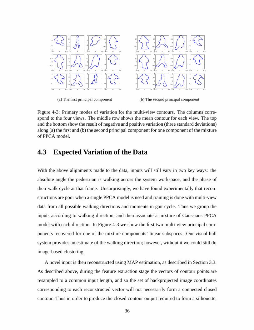
Figure 4-3: Primary modes of variation for the multi-view contours. The columns corre-spond to the four views. The middle row shows the mean contour for each view. The topand the bottom show the result of negative and positive variation (three standard deviations)along (a) the first and (b) the second principal component for one component of the mixtureof PPCA model.
4.3 Expected Variation of the Data
With the above alignments made to the data, inputs will still vary in two key ways: the
absolute angle the pedestrian is walking across the system workspace, and the phase of
their walk cycle at that frame. Unsurprisingly, we have found experimentally that recon-
structions are poor when a single PPCA model is used and training is done with multi-view
data from all possible walking directions and moments in gait cycle. Thus we group the
inputs according to walking direction, and then associate a mixture of Gaussians PPCA
model with each direction. In Figure 4-3 we show the first two multi-view principal com-
ponents recovered for one of the mixture components’ linear subspaces. Our visual hull
system provides an estimate of the walking direction; however, without it we could still do
image-based clustering.
A novel input is then reconstructed using MAP estimation, as described in Section 3.3.
As described above, during the feature extraction stage the vectors of contour points are
resampled to a common input length, and so the set of backprojected image coordinates
corresponding to each reconstructed vector will not necessarily form a connected closed
contour. Thus in order to produce the closed contour output required to form a silhouette,
36
we fit a spline to the image points corresponding to the reconstructed vector. To obtain
silhouettes from each reconstructed contour we simply perform a flood fill from the retained
centroid of the original input.
4.4 Results
According to the visual hull definition, missing pixels in a silhouette from one view are
interpreted as absolute evidence that all the 3D points on the ray corresponding to that
pixel are empty, irrespective of information in other views. Thus, segmentation errors may
have a dramatic impact on the quality of the 3D reconstruction. In order to examine how
well the reconstruction scheme we devised would handle this issue and improve 3D visual
hull approximations, we tested sets of views with segmentation errors due to erroneous
foreground/background estimates. We also synthetically imposed gross errors to test how
well our method can handle dramatic undersegmentations. Visual hulls are constructed
from the input views using the algorithm in [21].
The visual hull models resulting from the reconstructed views are qualitatively better
than those resulting from the raw silhouettes (see Figures 4-5, 4-6, 4-7, 4-8, 4-9, 4-10, 4-11,
and 4-12). Parts of the body which are missing in one input view do appear in the complete
3D approximation. Such examples illustrate the utility of modeling the uncertainty of an
observed contour.
In order to quantitatively evaluate how well our algorithm eliminates segmentation er-
rors, we obtained ground truth segmentations for a set of the multi-view pedestrian silhou-
ettes by manually segmenting the foreground body in each view. We randomly selected
32 frames (128 views) from our test set to examine in this capacity. The mean squared
error per contour point for the raw silhouettes in our ground truthed test set was found to
be approximately 40 pixels, versus 17 pixels for the reconstructed silhouettes. As shown in
the segmentation error distributions in Figure 4-4, the Bayesian reconstruction eliminates
the largest segmentation errors present in the raw images, and it greatly reduces the mean
error in most cases.
Using the RANSAC method described in Section 3.4, we reduced mean segmentation
37
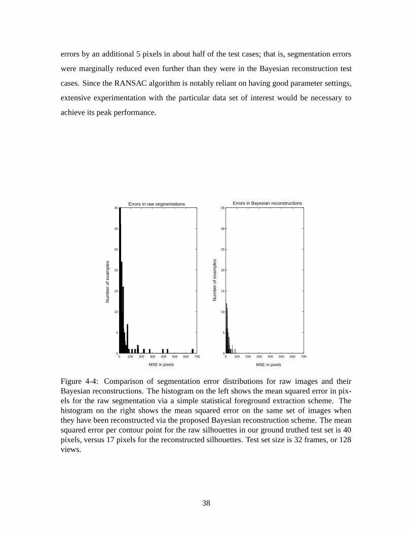
errors by an additional 5 pixels in about half of the test cases; that is, segmentation errors
were marginally reduced even further than they were in the Bayesian reconstruction test
cases. Since the RANSAC algorithm is notably reliant on having good parameter settings,
extensive experimentation with the particular data set of interest would be necessary to
achieve its peak performance.
0 100 200 300 400 500 600 7000
5
10
15
20
25
30
35Errors in raw segmentations
MSE in pixels
Num
ber
of e
xam
ples
0 100 200 300 400 500 600 7000
5
10
15
20
25
30
35Errors in Bayesian reconstructions
MSE in pixels
Num
ber
of e
xam
ples
Figure 4-4: Comparison of segmentation error distributions for raw images and theirBayesian reconstructions. The histogram on the left shows the mean squared error in pix-els for the raw segmentation via a simple statistical foreground extraction scheme. Thehistogram on the right shows the mean squared error on the same set of images whenthey have been reconstructed via the proposed Bayesian reconstruction scheme. The meansquared error per contour point for the raw silhouettes in our ground truthed test set is 40pixels, versus 17 pixels for the reconstructed silhouettes. Test set size is 32 frames, or 128views.
38

(a) Traditional construction (raw) (b) Bayesian reconstruction
Figure 4-5: An example of visual hull segmentation improvement with PPCA-basedBayesian reconstruction. The four top-left silhouettes show the multi-view input, corruptedby segmentation noise. The four silhouettes directly to their right show the correspondingBayesian reconstructions. In the gray sections below each set of silhouettes are their cor-responding visual hulls; the left VH is formed from the raw silhouettes, and the right VHis formed from the reconstructed silhouettes. Each model has been rotated in incrementsof 20 degrees so that the full 3D shape may be viewed. Finally, virtual frontal and pro-file views projected from the two VHs are shown at the bottom below their correspondingVHs. Note how undersegmentations in the raw input silhouettes cause portions of the ap-proximate 3D volume to be missing (left, gray background), whereas the reconstructedsilhouettes produce a fuller 3D volume more representative of the true object shape (right,gray background).
39

(a) Traditional construction (raw) (b) Bayesian reconstruction
Figure 4-6: An example of visual hull segmentation improvement with PPCA-basedBayesian reconstruction. See Figure 4-5 for explanation.
40
(a) Traditional construction (raw) (b) Bayesian reconstruction
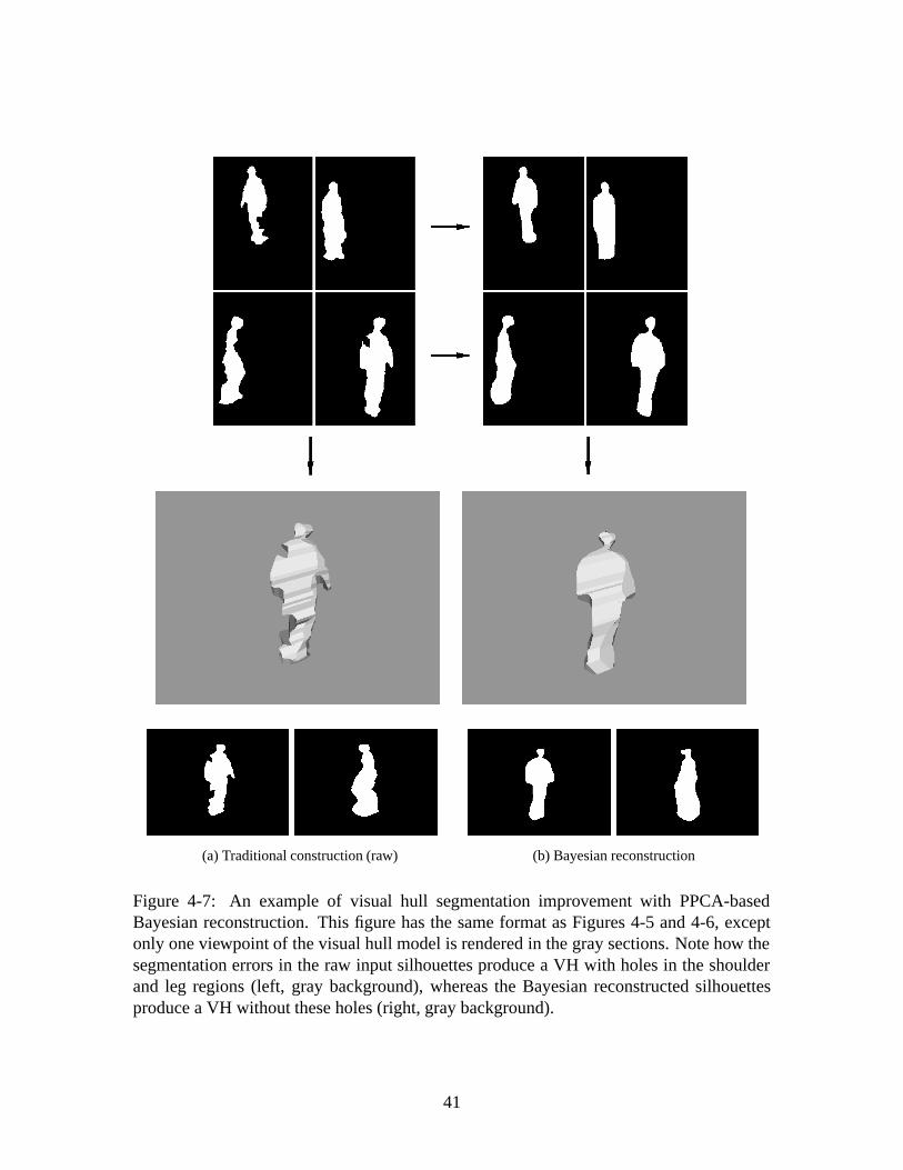
Figure 4-7: An example of visual hull segmentation improvement with PPCA-basedBayesian reconstruction. This figure has the same format as Figures 4-5 and 4-6, exceptonly one viewpoint of the visual hull model is rendered in the gray sections. Note how thesegmentation errors in the raw input silhouettes produce a VH with holes in the shoulderand leg regions (left, gray background), whereas the Bayesian reconstructed silhouettesproduce a VH without these holes (right, gray background).
41
(a) Traditional construction (raw) (b) Bayesian reconstruction
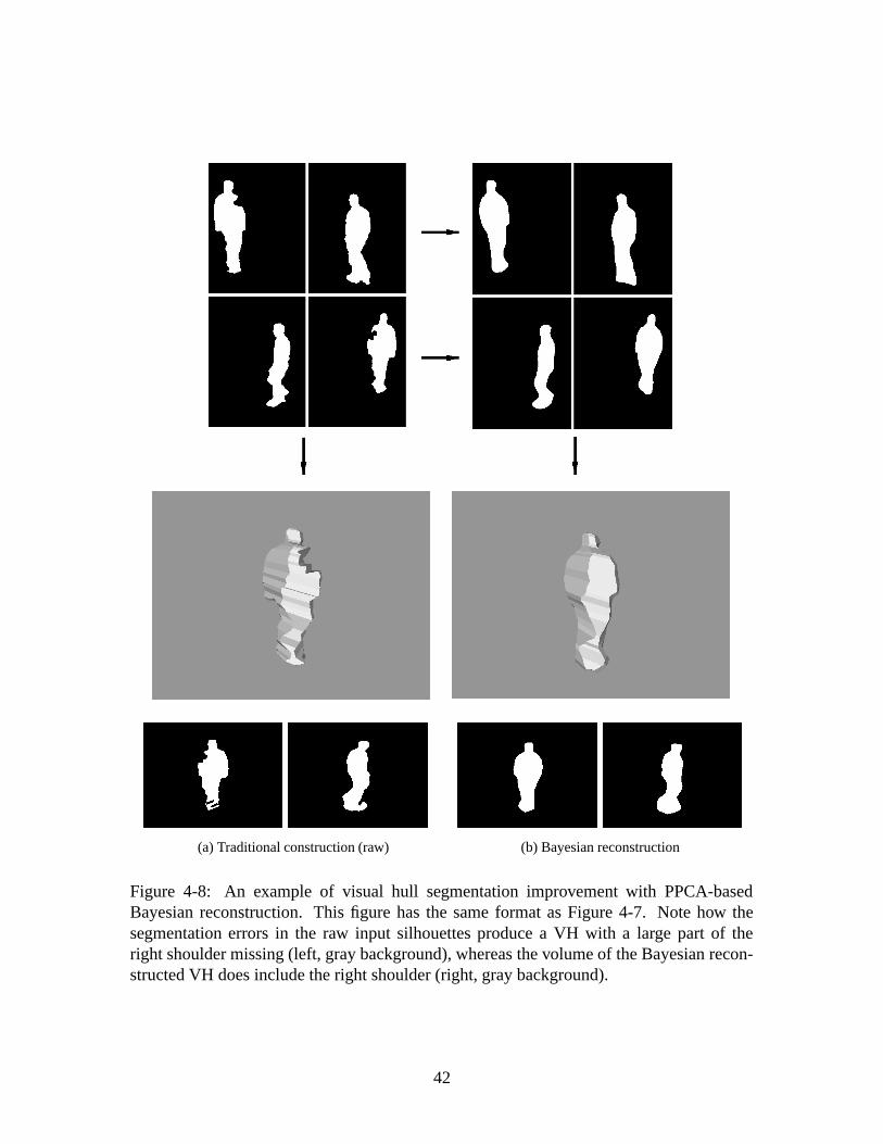
Figure 4-8: An example of visual hull segmentation improvement with PPCA-basedBayesian reconstruction. This figure has the same format as Figure 4-7. Note how thesegmentation errors in the raw input silhouettes produce a VH with a large part of theright shoulder missing (left, gray background), whereas the volume of the Bayesian recon-structed VH does include the right shoulder (right, gray background).
42

(a) Traditional construction (raw) (b) Bayesian reconstruction
Figure 4-9: An example of visual hull segmentation improvement with PPCA-basedBayesian reconstruction. This figure has the same format as the previous examples. Notehow the segmentation error in the raw input silhouettes results in a carved out portion of thechest in the VH (left, gray background); the chest is smoothly reconstructed in the Bayesianreconstructed VH (right, gray background).
43

(a) Traditional construction (raw) (b) Bayesian reconstruction
Figure 4-10: An example of visual hull segmentation improvement with PPCA-basedBayesian reconstruction. This figure has the same format as the previous examples. Notehow the segmentation error in the raw input silhouettes results in a carved out portion be-low the right shoulder and on the left leg in the VH (left, gray background); these holes arefilled in the Bayesian reconstructed VH (right, gray background).
44

(a) Traditional construction (raw) (b) Bayesian reconstruction
Figure 4-11: An example of visual hull segmentation improvement with PPCA-basedBayesian reconstruction. This figure has the same format as the previous examples. Notehow the segmentation error from the top-right raw input silhouette causes the carved outportion of the back in the raw VH (left, gray background), which is smoothly filled in forthe Bayesian reconstructed version (right, gray background). Also note how the right armis missing in the virtual frontal view produced by the raw VH (bottom, leftmost image),whereas the arm is present in the Bayesian reconstructed version (bottom, image secondfrom right).
45

(a) Traditional construction (raw) (b) Bayesian reconstruction
Figure 4-12: An example of visual hull segmentation improvement with PPCA-basedBayesian reconstruction. This figure has the same format as the previous examples. Notethe large missing portion of the torso in the 3D volume in the raw VH (left, gray back-ground), which is filled in for the Bayesian reconstructed version (right, gray background).Also note how the right shoulder is partially missing in the virtual frontal view producedby the raw VH (bottom, leftmost image), whereas the shoulder is intact in the reconstructedversion (bottom, image second from right).
46
Chapter 5
Inferring 3D Structure
In this chapter we desribe how to extend the shape model formulated in Chapter 3 to incor-
porate additional structural features.
5.1 Extending the Shape Model
The shape model can be augmented to include information about the object’s orientation
in the image, as well as the 3D locations of key points on the object. The mixture model
now represents a density over the observation space for the true underlying contours to-
gether with their associated 3D structure parameters. Novel examples are matched to the
contour-based shape model using the same multi-view reconstruction method described in
Chapter 3 in order to infer their unknown or missing parameters. (See Figure 5-1 for a
diagram of data flow.)
The shape model is trained on a set of vectors that are composed of points from multiple
contours from simultaneous views, plus a number of three-dimensional structure parame-
ters, sj = (s1j , s
2j , s
3j). The observation vector on is then defined as
on = (c1, c2, ..., cK, s1, s2, ..., sz)T (5.1)
where there are z 3D points for the structure parameters. When presented with a new multi-
view contour, we find the MAP estimate of the shape and structure parameters based on
47

Reconstructedsilhouettes
structure parameters
Reconstruction viaprobabilistic shape model
parameters3D structure
Inference of 3D
Sampled, normalizedcontour points
Silhouettes
Multi-viewtextured images
subtractionBackground
Contour pointsplus 3D structure
parameters
Synthetictraining images
PPCA models
EM
Figure 5-1: Diagram of data flow: using the probabilistic shape model for 3D structureinference.
only the observable contour data. The training set for this inference task may be comprised
of real or synthetic data.
5.2 Advantages of the Model
One strength of the proposed approach for the estimation of 3D feature locations is that
the silhouettes in the novel inputs need not be cleanly segmented. Since the contours and
unknown parameters are reconstructed concurrently, the parameters are essentially inferred
from a restricted set of feasible shape reconstructions; they need not be determined by an
explicit match to the raw observed silhouettes. Therefore, the probabilistic shape model
does not require an expensive segmentation module. A fast simple foreground extraction
scheme is sufficient.
As should be expected, our parameter inference method also benefits from the use of
multi-view imagery (as opposed to single-view). Multiple views will in many cases over-
come the ambiguities that are geometrically inherent in single-view methods.
Our model allows structure to be inferred using only directly observable features in
multi-view images; no explicit shape model is constructed. Moreover, we do not require
that any class-specific a priori kinematic or shape constraints be explicitly specified. The
48

only prior information utilized is learned directly from extracted contours, and structure
parameters may be learned from a synthetic training set, as we will describe in Section 6.2.
Model matching consists of one efficient reconstruction step. No iterative search or fitting
scheme is needed.
49

50
Chapter 6
Inferring 3D Structure in Pedestrian
Images
We have applied our method to a data set of multi-view images of people walking. The
goal is to infer the 3D positions of joints on the body given silhouette views from different
viewpoints. For a description of the imaging model used in the experiments in this chapter,
see Section 4.1.
6.1 Advantages of a Synthetic Training Set
A possible weakness of any shape model defined by examples is that the ability to accu-
rately represent the space of realizable shapes will generally depend heavily on the amount
of available training data. Moreover, we note that the training set on which the probabilistic
shape + structure model is learned must be “clean”; otherwise the model could fit the bias
of a particular segmentation algorithm. It must also be labeled with the true values for the
3D features. Collecting a large data set with these properties would be costly in resources
and effort, given the state of the art in motion capture and segmentation, and at the end the
“ground truth” could still be imprecise. We chose therefore to use realistic synthetic data
for training a multi-view pedestrian shape model. We obtained a large training set by using
POSER [8] – a commercially available animation software package – which allows us to
manipulate realistic humanoid models, position them in the simulated scene, and render
51

00.20.4
0
0.1
0.2
0.3
0.4
0.5
0.6
0 0.1 0.2
lw
le
ls
lk
lt
la
ltoe
n
th
bh
ra
rt
rtoe
rk
rs
re
rw
Figure 6-1: An example of synthetically generated training data. Textured images (top)show rendering of example human model, silhouettes and stick figure (below) show multi-view contours and structure parameters, respectively.
textured images or silhouettes from a desired point of view. Our goal is to train the model
using this synthetic data, but then use the model for reconstruction and inference tasks with
real images.
6.2 Description of the Training Set
We generated 20,000 synthetic instances of multi-view input for our system. For each
instance, a humanoid model was created with randomly adjusted anatomical shape param-
eters, and put into a walk-simulating pose, at a random phase of the walking cycle. The
orientation of the model was drawn at random as well in order to simulate different walk di-
rections of human subjects in the scene. Then for each camera in the real setup we rendered
a snapshot of the model’s silhouette from a point in the virtual scene approximately corre-
sponding to that camera. In addition to the set of silhouettes, we record the 3D locations
of 19 landmarks of the model’s skeleton, corresponding to selected anatomical joints. (See
Figure 6-1.) We used POSER’s scripting language, Python, in order to generate this large
number of examples with randomly varying parameters with minimal human interaction.
52
6.3 Representation for the Extended Shape Model
For this extended model, each silhouette is again represented as sampled points along the
closed contour of the largest connected component extracted from the original binary im-
ages. All contour points are normalized to a translation and scale invariant input coordinate
system, and each vector of normalized points is resampled to a common vector length using
nearest neighbor interpolation. The complete representation is then the vector of concate-
nated multi-view contour points plus a fixed number of 3D body part locations (see Equa-
tion (5.1)). In the input observation vector for each test example, the 3D pose parameters
are set to zero.
6.4 Description of the Synthetic Test Set
Since we do not have ground truth pose parameters for the raw test data, we have tested a
separate, large, synthetic test set with known pose parameters so that we can obtain error
measurements for a variety of experiments. In order to evaluate our system’s robustness
to mild changes in the appearance of the object, we generated test sequences in the same
manner as the synthetic training set was generated, but with different virtual characters,
i.e., different clothing, hair and body proportions. To make the synthetic test set more
representative of the real, raw silhouette data, we added noise to the contour point locations.
Noise is added uniformly in random directions, or in contiguous regions along the contour
in the direction of the 2D surface normal. Such alterations to the contours simulate the
real tendency for a simple background subtraction mechanism to produce holes or false
extensions along the true contour of the object. (See Figure 6-2.)
53

Figure 6-2: Noisy synthetic test silhouettes. Top images show clean synthetic silhouettes.Images below them show same silhouettes with noise added to image coordinates of con-tour points. Left example has uniform noise; right example has nonuniform noise in patchesnormal to contour.
6.5 Results
6.5.1 Error Measures
The pose error ef for each test frame is defined as the average distance in centimeters
between the estimated and true positions of the 19 joints,
ef =1
19
∑
i
|ei|, (6.1)
where ei is the individual error for joint i.
As described above, test silhouettes are corrupted with noise and segmentation errors
so that they may be more representative of real, imperfect data, yet still allow us to do a
large volume of experiments with ground truth. The “true” underlying contours from the
clean silhouettes (i.e., the novel silhouettes before their contour points were corrupted) are
saved for comparison with the reconstructed silhouttes. The contour error for each frame
is then the distance between the true underlying contours and their reconstructions.
54

Contour error is measured using the Chamfer distance. For all pixels with a given
feature (usually edges, contours, etc.) in the test image I, the Chamfer distance D measures
the average distance to the nearest feature in the template image T.
D(T, I) =1
N
∑
f∈T
dT (f) (6.2)
where N is the number of pixels in the template where the feature is present, and dT (f) is
the distance between feature f in T and the closest feature in I.
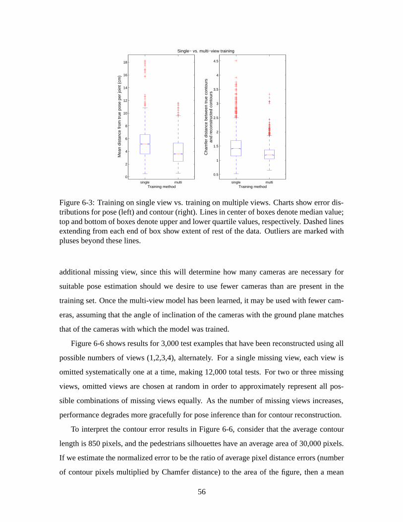
6.5.2 Training on One View Versus Training on Multiple Views
Intuitively, a multi-view framework can discern 3D poses that are inherently ambiguous in
single-view images. Our experimental results validate this assumption. We performed par-
allel tests for the same examples, in one case using our existing multi-view framework, and
in the other, using the framework outlined above, only with the model altered to be trained
and tested with single views alone. Figure 6-3 compares the overall error distributions of
the single and multi-view frameworks for a test set of 3,000 examples. Errors in both pose
and contours are measured for both types of training. Multi-view reconstructions are con-
sistently more accurate than single-view reconstructions. Training the model on multi-view
images yields on average 24% better pose inference performance and 16% better contour
reconstruction performance than training the model on single-view images.
6.5.3 Testing with Missing Views
We have also tested the performance of our multi-view method applied to body pose esti-
mation when only a subset of views is available for reconstruction. A missing view in the
shape vector is represented by zeros in the elements corresponding to that view’s resampled
contour. Just as unknown 3D locations are inferred for the test images, our method recon-
structs the missing contours by inferring the shape seen in that view based on examples
where all views are known. (See Figures 6-4, 6-5, 6-6, 6-7, 6-8, 6-9, and 6-10.)
We are interested in knowing how pose estimation performance degrades with each
55
single multi
0
2
4
6
8
10
12
14
16
18
Single− vs. multi−view training
Mea
n di
stan
ce fr
om tr
ue p
ose
per
join
t (cm
)
Training methodsingle multi
0.5
1
1.5
2
2.5
3
3.5
4
4.5
Cha
mfe
r di
stan
ce b
etw
een
true
con
tour
san
d re
cons
truc
ted
cont
ours
Training method
Figure 6-3: Training on single view vs. training on multiple views. Charts show error dis-tributions for pose (left) and contour (right). Lines in center of boxes denote median value;top and bottom of boxes denote upper and lower quartile values, respectively. Dashed linesextending from each end of box show extent of rest of the data. Outliers are marked withpluses beyond these lines.
additional missing view, since this will determine how many cameras are necessary for
suitable pose estimation should we desire to use fewer cameras than are present in the
training set. Once the multi-view model has been learned, it may be used with fewer cam-
eras, assuming that the angle of inclination of the cameras with the ground plane matches
that of the cameras with which the model was trained.
Figure 6-6 shows results for 3,000 test examples that have been reconstructed using all
possible numbers of views (1,2,3,4), alternately. For a single missing view, each view is
omitted systematically one at a time, making 12,000 total tests. For two or three missing
views, omitted views are chosen at random in order to approximately represent all pos-
sible combinations of missing views equally. As the number of missing views increases,
performance degrades more gracefully for pose inference than for contour reconstruction.
To interpret the contour error results in Figure 6-6, consider that the average contour
length is 850 pixels, and the pedestrians silhouettes have an average area of 30,000 pixels.
If we estimate the normalized error to be the ratio of average pixel distance errors (number
of contour pixels multiplied by Chamfer distance) to the area of the figure, then a mean
56

rw re
rs
rtoe
rk
ra
rt
bh th n
lt
ltoe la
lk
ls le lw
la
re
ltoe
rs
ra
rt
rk
rw
n
lt
th
rtoe
bh
le lw
ls
lk
la ltoe
lw le
ra
rt
rs
lt
ls n
re
lk
th bh
rk
rtoe
rw lw le
ls
lk
ltoe
lt
la
n bh th
rt
ra
rk
rtoe
rs
rw re
Figure 6-4: Inferring structure from only a single view. Top row shows ground truth silhou-ettes that are not in the training set. Noise is added to input contour points of second view(middle), and this single view alone is matched to the multi-view shape model in orderto infer the 3D joint locations (bottom, solid blue) and compare to ground truth (bottom,dotted red). Abbreviated body part names appear by each joint. This is an example withaverage pose error of 5 cm.
57

le
la
lw
ltoe
lk
ls
lt
ra
n bh
rt
rtoe
th
rk
rw re rs
lw
rtoe
le
ra
ls
rk
th
bh n
lt rt
rs
lk
ltoe
re
la
rw
rtoe ra
rk
lw
th
bh
le
n rs
rt
ls
lt
re
ltoe
rw
lk
la rtoe
rs
rk
re
ra
rw rt
th
bh n
lt
ltoe
lw
lk
ls
la
le
Figure 6-5: Inferring structure with one missing view. Top row shows noisy input silhou-ettes, middle row shows contour reconstructions, and bottom row shows inferred 3D jointlocations (solid blue) and ground truth pose (dotted red). This is an example with aver-age pose error of 2.5 cm per joint and an average Chamfer distance from the true cleansilhouettes of 2.3.
58

0 1 2 3
0
5
10
15
20
25
30
Pose error
Mea
n di
stan
ce fr
om tr
ue p
ose
per
join
t (cm
)
Number of missing views0 1 2 3
2
4
6
8
10
12
Contour reconstruction error
Cha
mfe
r di
stan
ce b
etw
een
true
con
tour
san
d re
cons
truc
ted
cont
ours
Number of missing views
Figure 6-6: Missing view results. Charts show distribution of errors for pose (left) andcontours (right) when model is trained on four views, but only a subset of views is availablefor reconstruction. Plotted as in Figure 6-3.
Chamfer distance of 1 represents an approximate overall error of 2.8%, distances of 4
correspond to 11%, etc. Given the large degree of segmentation errors imposed on the test
sets, these are acceptable contour errors in the reconstructions, especially since the 3D pose
estimates (our end goal in this setting) do not suffer proportionally.
6.5.4 Testing on Real Data
Finally, we evaluated our algorithm on a large data set of real images of pedestrians taken
from a database of 4,000 real multi-view frames. The real camera array is mounted on the
ceiling of an indoor lab environment. The external parameters of the virtual cameras in the
graphics software that were used for training are roughly the same as the parameters of this
real four-camera system. The data contains 27 different pedestrian subjects.
Sample results for the real test data set are shown in Figures 6-7, 6-8, 6-9, and 6-10.
The original textured images, the extracted silhouettes, and the inferred 3D pose are shown.
Without having point-wise ground truth for the 3D locations of the body parts, we can best
assess the accuracy of the inferred pose by comparing the 3D stick figures to the original
59

textured images. To aid in inspection, the 3D stick figures are rendered from manually
selected viewpoints so that they are approximately aligned with the textured images.
6.5.5 Results Summary
In summary, our experiments show how the shape + structure model we have formulated
is able to infer 3D structure by matching observed image features directly to the model.
Our tests with a large set of noisy, ground-truthed synthetic images offer evidence of the
ability of our method to infer 3D parameters from contours, even when inputs have seg-
mentation errors. In the experiments shown in Figure 6-6, structure inference for body pose
estimation is accurate within 3 cm on average. Performance is good even when there are
fewer views available than were used during training; with only one input view, pose is still
accurate within 15 cm on average, and can be as accurate as within 4 cm. Finally, we have
successfully applied our synthetically-trained model to real data and a number of different
subjects.
60

ra rtoe
rk
re
rs
rt rw
n
th
bh
lt
le
ls
lw
la
lk
ltoe ra rtoe
rk
le
lw
ls
rt lt
rs n
re
th
bh
la
lk
rw
ltoe
le
lw
ls
ra
lt
rtoe la
lk
n
th
bh
ltoe
rk
rt
rs
re
rw
ltoe
lk
la
ls
lw
le
lt
bh
th
n
rw rt
rs
re
rk
rtoe ra
rw
ltoe
re
la
rs
lk
rt
bh th
n
rk
lt
rtoe
ls
ra
le
lw
ra rtoe
rk
re
rs
rt rw
n
le
th bh
lt lw
ls
la
lk
ltoe ra
rtoe
rk
le
lw rt
ls
lt
rs n
th bh
re rw
lk
la ltoe
lw
le
ls
lt
lk
n bh th
la ra ltoe rtoe
rt
rk
rs
re rw
Figure 6-7: Inferring structure on real data. For each example, top row shows original tex-tured multi-view image, middle row shows extracted input silhouettes where the views thatare not used in reconstruction are omitted, and bottom row shows inferred joint locationswith stick figures rendered at different viewpoints. To aid in inspection, the 3D stick figuresare rendered from manually selected viewpoints that were chosen so that they are approxi-mately aligned with the textured images. In general, estimation is accurate and agrees withthe perceived body configuration. An example of an error in estimation is shown in the topleft example’s left elbow, which appears to be incorrectly estimated as bent.
61

la
le
lk
ls
lw lt
ltoe ra
n
rt
bh th
rtoe
rk
rw re rs
rtoe
lw le
ra
ls
rk
lt
lk
th bh n
rt
ltoe
rw
rs
re
la rtoe
rk
ra
rs
th bh
rt lw
n
re rw
le ls
lt
lk
ltoe la
re
rs
rw
rk rt
ltoe
rtoe ra
la
bh n th
lk
lt
ls
lw le
re
la
rs
rw
ltoe
rt
rk
ra
n
th
bh
rtoe
lt
lk
ls
le
lw
la ltoe ra
rs
rt
re le
lt
lk
lw
ls n
rk
th
bh
rw
rtoe
la
le
lw
ltoe
ls
lk
lt
ra
n bh
th
rt
rtoe
rk
rs
re
rw lw
le
ls
lk
rtoe
lt
ra ltoe
bh n
th
rk
la
rt rw
rs
re
Figure 6-8: Inferring structure on real data with two missing views. See caption of Figure 6-7 for explanation.
62
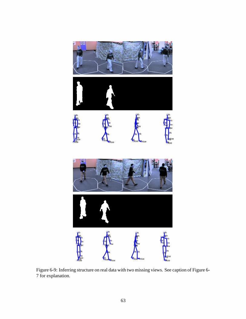
le
ls
lw
lk
lt
la ltoe
n th bh
rt
ra
rw
rk
rs re
rtoe rtoe
lw le
ra
ls
rk
lt
th bh n
lk
rt
rs
rw
ltoe
re
la rtoe ra
rk
lw
th bh
le
n
rt
ls rs
lt rw re
lk
ltoe la
re
rs
rw
rk
rtoe
rt
ra
bh
ltoe
th
n
la
lt
lk
lw
ls le
le
lw
ls
lk
la
lt
ltoe ra
n bh th
rt
rtoe
rk
rw re rs
rtoe
lw
le
ra
ls
rk
lt
th bh n
lk
rt
rs
ltoe
rw
re
la rtoe ra
rk
lw
th bh n
le
ls
rt
rs
lt re rw
lk
ltoe la
re rw
rs
rk
rtoe
rt
ltoe ra la
bh n
th
lk
lt lw
ls le
Figure 6-9: Inferring structure on real data with two missing views. See caption of Figure 6-7 for explanation.
63

lw le
ls
lk
lt
ltoe la
n bh th
rtoe ra
rt
rk
rs
re
rw
rk
lw
rs
th bh
rtoe
rt
n
ltoe
re le
lt
ls
rw
lk
ra la
rs
rk
re
rw
th
bh
rt
n
rtoe
lw
ra ltoe
lt
ls
lk
le
la
rw
re
rs
ra
rt
rk
rtoe la
n
th
bh
ltoe
lt
lk
ls
le lw
lw
rtoe
le
ls
ra
rk
lt
th
bh n
lk
rt
rs
ltoe la
re
rw
rtoe
rk
lw
rs
ra
th
bh
rt
n
re
rw
le
lt
ltoe
ls
lk
la
re
rs
rw
rk
rt
rtoe ltoe ra
bh
th
n
la
lk
lt lw
ls
le
la
rw
re
ltoe
lk
rs
lt rt
n ls bh
th
ra
le
rk
lw
rtoe
Figure 6-10: Inferring structure on real data from only a single view. See caption of Fig-ure 6-7 for explanation.
64

Chapter 7
Conclusions and Future Work
We have developed a Bayesian approach to visual hull reconstruction using an image-based
representation of 3D object shape, as well as an image-based approach to infer 3D structure
parameters. We have shown how the use of a class-specific prior in visual hull reconstruc-
tion reduces the effect of segmentation errors in the silhouette extraction process. We have
also demonstrated how the use of our shape model and Bayesian reconstruction technique
enables accurate estimation of structure parameters in spite of large segmentation errors
or even missing views in the input silhouettes. Novel examples with contour information
but unknown 3D point locations are matched to the model in order to retrieve estimates
for unknown parameters. Model matching and parameter inference are done entirely in the
image domain and require no explicit 3D construction from multiple views.
Our method was applied to a data set of pedestrian sequences, and improvements in the
approximate 3D models under various noise conditions were shown. We have also reported
pose and contour error measures on a large set of noisy synthetic images of pedestrians.
We note again that while the experiments we present in this work deal with a data set of
pedestrian images, the shape model and reconstruction method we propose have no inherent
specification for this particular object class. The methods we present are intended for use
on any class of objects for which the global shape is roughly similar across instances of the
class.
In future work we will explore non-parametric density models for inferring structure
from shape. We plan to further test our method to see if our model improves accuracy in
65

applications that use a visual hull for view synthesis in recognition tasks. We also plan to
run experiments using motion capture data so that we may compare real image test results
to ground-truth joint angles. In addition, we intend to include dynamics to strengthen our
model for the pedestrian walking sequences. We are also interested in how the body pose
estimation application may be utilized in a higher-level gesture or gait recognition system.
66

Appendix A
Random Sample Consensus (RANSAC)
for Multi-View Contour Reconstruction
We adapted the Random Sample Consensus (RANSAC) algorithm to make it suitable for
the robust reconstruction of multi-view contours. The algorithm iteratively seeks to remove
the outlier points present in the input contours. Only the “inlier” points are used to perform
the Bayesian reconstruction. The RANSAC variant we have devised is given in Figure A-1.
Random samples of contour points are drawn from each view in succession, and the points
from each view which result in the best fitting reconstruction are used in the final Bayesian
multi-view reconstruction.
67

Determine parameters:N - the smallest number of points required to compose
a contour in one view.W - the number of iterations required.T - the threshold used to identify if a point fits well.D - the number of nearby points required to assert that
model fits well.
For each of the K views:
For W iterations:
Draw a sample of N points from the raw inputcontour in the current view.
Form Bayesian multi-view reconstruction using thatsubset of points, using all contour points in theother K-1 views.
Compute distance transform for the current view.
For each point from the current view’s raw inputcontour that is not in the sampled subset:
If distance from that point to the reconstructedcontour is less than or equal to threshold T,then that point is deemed close.
end
If there are D points close to the reconstructedcontour, then there is a good fit. Reconstructthe multi-view contour replacing the current viewwith the sampled N points plus the D or moreclose points.
Calculate the fitting error for the new reconstruction,defined as the Chamfer distance between the raw inputcontour and the Bayesian reconstructed contour.
end
Save the points for the current view that had thelowest fitting error.
end
Reconstruct the multi-view contour using the inlierpoints saved from each view.
Figure A-1: RANSAC variant for robust reconstruction of multi-view contours.
68

Bibliography
[1] A. Baumberg and D. Hogg. Learning Flexible Models from Image Sequences. In
Proceedings of European Conference on Computer Vision, Stockholm, Sweden, May
1994.
[2] A. Baumberg and D. Hogg. An Adaptive Eigenshape Model. In British Machine
Vision Conference, pages 87–96, Birmingham, England, September 1995.
[3] M. Carreira-Perpinan. Mode-Finding for Mixtures of Gaussian Distributions. IEEE
Transactions on Pattern Analysis and Machine Intelligence, 22(11):1318–1323,
November 2000.
[4] T. F. Cootes and C. J. Taylor. A Mixture Model for Representing Shape Variation. In
British Machine Vision Conference, pages 110–119, Essex, England, 1997.
[5] T. F. Cootes, C. J. Taylor, D. H. Cooper, and J. Graham. Active Shape Models - Their
Training and Application. Computer Vision and Image Understanding, 61(1):38–59,
January 1995.
[6] T.F. Cootes, G.V. Wheeler, K.N. Walker, and C.J. Taylor. View-Based Active Appear-
ance Models. Image and Vision Computing, 20:657–664, 2002.
[7] M. Covell. Eigen-Points: Control-Point Location Using Principal Component Anal-
ysis. In Proceedings of the IEEE International Conference on Automatic Face and
Gesture Recognition, pages 122–127, Killington, Vermont, October 1996.
[8] Egisys Co. Curious Labs. Poser 5 : The Ultimate 3D Character Solution. 2002.
69

[9] D. A. Forsyth and J. Ponce. Computer Vision: A Modern Approach, chapter 15.5,
pages 346–348. Prentice Hill, Upper Saddle River, New Jersey, 2003.
[10] H. Freeman. On the Encoding of Arbitrary Geometric Configurations. IRE Trans.
Electron. Comput., EC-10:260–268, June 1961.
[11] D. Gavrila. The Visual Analysis of Human Movement: A Survey. Computer Vision
and Image Understanding, 73(1):82–98, 1999.
[12] J. Haslam, C. J. Taylor, and T. F. Cootes. A Probabilistic Fitness Measure for De-
formable Template Models. In British Machine Vision Conference, pages 33–42,
York, England, September 1994.
[13] M. Isard and A. Blake. Condensation – Conditional Density Propagation for Visual
Tracking. International Journal of Computer Vision, 29(1):5–28, 1998.
[14] M. Jones and T. Poggio. Multidimensional morphable models. In Proceedings of
the International Conference on Computer Vision, pages 683–688, Bombay, India,
January 1998.
[15] M. Kass, A. Witkin, and D. Terzopoulos. Snakes: Active Contour Models. Interna-
tional Journal of Computer Vision, 1(4):321–332, 1988.
[16] K. N. Kutulakos and S. M. Seitz. A Theory of Shape by Space Carving. International
Journal of Computer Vision, 38(3):199–218, 2000.
[17] A. Laurentini. The Visual Hull Concept for Silhouette-Based Image Understanding.
IEEE Transactions on Pattern Analysis and Machine Intelligence, 16(2):150–162,
February 1994.
[18] S. Lazebnik, E. Boyer, and J. Ponce. On Computing Exact Visual Hulls of Solids
Bounded by Smooth Surfaces. In Proceedings IEEE Conference on Computer Vision
and Pattern Recognition, pages 156–161, Lihue, Hawaii, December 2001.
70

[19] M. Leventon, W. E. L. G. Grimson, and O. Faugeras. Statistical Shape Influence in
Geodesic Active Contours. In Proceedings IEEE Conference on Computer Vision and
Pattern Recognition, pages 316–323, Hilton Head Island, South Carolina, June 2000.
[20] W. Matusik, C. Buehler, and L. McMillan. Polyhedral Visual Hulls for Real-Time
Rendering. In Proceedings of Eurographics Workshop on Rendering, pages 115–126,
London, England, June 2001.
[21] W. Matusik, C. Buehler, R. Raskar, S. Gortler, and L. McMillan. Image-Based Vi-
sual Hulls. In Proceedings ACM Conference on Computer Graphics and Interactive
Techniques, pages 369–374, 2000.
[22] W. Matusik, H. Pfister, A. Ngan, P. Beardsley, R. Ziegler, and L. McMillan. Image-
Based 3D Photography Using Opacity Hulls. In Proceedings ACM Conference on
Computer Graphics and Interactive Techniques, pages 427–437, New York, July
2002.
[23] B. Moghaddam. Principal Manifolds and Probabilistic Subspaces for Visual Recog-
nition. IEEE Transactions on Pattern Analysis and Machine Intelligence, 24(6):780–
788, June 2002.
[24] Netlab. http://www.ncrg.aston.ac.uk/netlab/index.html.
[25] E-J. Ong and S. Gong. The Dynamics of Linear Combinations. Image and Vision
Computing, 20(5–6):397–414, 2002.
[26] S. M. Seitz and C. R. Dyer. Photorealistic Scene Reconstruction by Voxel Coloring.
International Journal of Computer Vision, 35(2):151–173, 1999.
[27] G. Shakhnarovich, L. Lee, and T. Darrell. Integrated Face and Gait Recognition From
Multiple Views. In Proceedings IEEE Conference on Computer Vision and Pattern
Recognition, Lihue, Hawaii, December 2001.
[28] D. Snow, P. Viola, and R. Zabih. Exact Voxel Occupancy with Graph Cuts. In
Proceedings IEEE Conference on Computer Vision and Pattern Recognition, pages
345–353, Hilton Head Island, South Carolina, June 2000.
71

[29] M. Tipping and C. Bishop. Mixtures of Probabilistic Principal Component Analyzers.
Neural Computation, 11(2):443–482, 1999.
[30] M. Turk and A. Pentland. Face Recognition Using Eigenfaces. In Proceedings IEEE
Conference on Computer Vision and Pattern Recognition, pages 586–590, Maui,
Hawaii, June 1991.
[31] Y. Wang and L. H. Staib. Boundary Finding with Prior Shape and Smoothness Mod-
els. IEEE Transactions on Pattern Analysis and Machine Intelligence, 22(7):738–743,
2000.
[32] K-Y. K. Wong and R. Cipolla. Structure and Motion from Silhouettes. In Proceed-
ings of the International Conference on Computer Vision, pages 217–222, Vancouver,
Canada, July 2001.
72
Recommended