A Simple Method for Detecting Interactions between a
Treatment and a Large Number of Covariates
Lu Tian ∗
Ash A Alizadeh †
Andrew J Gentles ‡
and
Robert Tibshirani§
March 8, 2014
Abstract
We consider a setting in which we have a treatment and a potentially large number
of covariates for a set of observations, and wish to model their relationship with an
outcome of interest. We propose a simple method for modeling interactions between
the treatment and covariates. The idea is to modify the covariate in a simple way,
and then fit a standard model using the modified covariates and no main effects. We
show that coupled with an efficiency augmentation procedure, this method produces
clinically meaningful estimators in a variety of settings. It can be useful for practic-
ing personalized medicine: determining from a large set of biomarkers the subset of
∗Depts. of Health, Research & Policy, 94305, [email protected]†Dept. of Medicine, Stanford University. 94305, [email protected]‡Integrative Cancer Biology Program, Stanford University. [email protected]§Depts. of Health, Research & Policy, and Statistics, Stanford University, [email protected]
1

patients that can potentially benefit from a treatment. We apply the method to both
simulated datasets and real trial data. The modified covariates idea can be used for
other purposes, for example, large scale hypothesis testing for determining which of a
set of covariates interact with a treatment variable.
1 Introduction
To develop strategies for personalized medicine, it is important to identify the treatment and
covariate interactions in the setting of randomized clinical trials [Royston and Sauerbrei,
2008]. To confirm and quantify the treatment effect is often the primary objective of a
randomized clinical trial. Although important, the final result (positive or negative) of a
randomized trial is a conclusion with respect to the average treatment effect on the entire
study population. For example, a treatment may not be different from the placebo in the
overall study population, but it may still be better for a subset of patients. Identifying the
treatment and covariate interactions may provide valuable information for determining this
subgroup of patients.
In practice, there are two commonly used approaches to characterize the potential treat-
ment and covariate interactions. First, a panel of simple patient subgroup analyses, where
the treatment and control arms are compared in different patient subgroups defined a priori,
such as male, female, diabetic and non-diabetic patients, may be performed following the
main comparison. Such an exploratory approach is mainly focusing on simple interactions
between treatment and a dichotomized covariate. However it often suffers from false pos-
itive findings due to multiple testings and can not find complicated treatment-covariates
interaction.
In a more rigorous analytic approach, the treatment-covariates interactions can be exam-
ined in a multivariate regression analysis where the product of the binary treatment indicator
2

and a set of baseline covariates are included in the regression model. Recent breakthroughs
in biotechnology make a vast amount of data available for exploring potential interaction
effects with the treatment and assisting in the optimal treatment selection for individual
patients. However, it is very difficult to detect the interactions between treatment and high
dimensional covariates via the direct multivariate regression modeling. Appropriate vari-
able selection methods such as Lasso are needed to reduce the number of covariates having
interactions with the treatment. The presence of the main effect, which often have bigger
effect on the outcome than the treatment interactions, further compounds the difficulty in
dimension reduction since a subset of variables need to be selected for modeling the main
effect as well.
Recently, Bonetti and Gelber [2004] formalized the subpopulation treatment effect pat-
tern plot (STEPP) for characterizing interactions between the treatment and continuous
covariates. Sauerbrei et al. [2007] proposed an efficient algorithm for multivariate model-
building with flexible fractional polynomials interactions (MFPI) and compared the empirical
performance of MFPI with STEPP. Su et al. [2008] proposed the classification and regression
tree method to explore the covariates and treatment interactions in survival analysis. Tian
and Tibshirani [2010] proposed an efficient algorithm to construct an index score, the sum of
selected dichotomized covariates, to stratify the patient population according to the treat-
ment effect. In a more recent work, Zhao et al. [2012] proposed a novel approach to directly
estimate the optimal treatment selection rule via maximizing the expected clinical utility,
which is equivalent to a weighted classification problem. There are also rich Bayesian liter-
atures for flexible modeling nonlinear, nonadditive or interaction covariate effects [LeBlanc,
1995, Chipman et al., 1998, Gustafson, 2000, Chen et al., 2012]. However, most of these
existing methods except for the one proposed by Zhao et al. [2012], are not designed to deal
with high-dimensional covariates.
In this paper, we propose a simple approach to estimate the covariates and treatment
3

interactions without the need for modeling the main effects in analyzing data from a ran-
domized clinical trial. The idea is simple, and in a sense, obvious. We simply code the
treatment variable as ±1 and then include the products of this variable with each covariate
in an appropriate regression model.
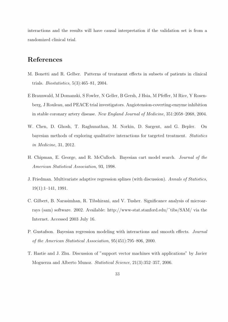
Figure 1 gives a preview of the results of our method. The data consist of baseline
covariates including various biomarker measurements and medical history for patients with
stable coronary artery disease and normal or slightly reduced left ventricular function, who
were randomized to either the angiotensin converting enzyme(ACE) inhibitor or placebo arm.
Our proposed method constructs a numerical score using baseline information on a training
set to reveal covariates-treatment interactions. The panels show the estimated survival
curves for patients in a separate validation set, overall and stratified by the score. Although
there is no significant survival difference between two arms in the overall comparison (hazard
ratio=0.95, p = 0.67), we see that patients with low scores have better survival with the
ACE inhibitor treatment than with the placebo (hazard ratio=0.74, p = 0.06). This type of
information after appropriate validation could be very useful in clinical practice.
In section 2, we describe the methods for the continuous, binary as well as survival type
of outcomes. We also establish a simple casual interpretation of the proposed method in
several cases. In section 3, the finite sample performance of the proposed method has been
investigated via extensive numerical studies. In section 4, we apply the proposed method
to two real data examples. Finally, limitation and potential extensions of the method are
discussed in section 5.
2 Method
In the following, we let T = ±1 be the binary treatment indicator and Y (1) and Y (−1) be
the potential outcome if the patient received treatment T = 1 and −1, respectively. We
4

only observe Y = Y (T ), T and Z, a q−dimensional baseline covariate vector. Here we
assume that the treatment is randomly assigned to a patient, i.e., T and Z are independent.
The observed data consist of N independent and identically distributed copies of (Y, T,Z),
{(Yi, Ti,Zi), i = 1, · · · , N}. Furthermore, we let W(·) : Rq → Rp be a p dimensional functions
of baseline covariates Z and always include an intercept. In practice, W(·) may include spline
basis functions and interactions selected by the users. We denote W(Zi) by Wi in the rest
of the paper. Here the dimension of Wi could be large relative to the sample size N. For
simplicity, we assume that Prob(T = 1) = Prob(T = −1) = 1/2.
2.1 Continuous Response Model
When Y is a continuous response, a simple multivariate linear regression model for charac-
terizing the interactions between the treatment and covariates is
Y = β′0W(Z) + γ ′0W(Z) · T/2 + ε, (1)
where ε is the mean zero random error. In this simple model, the interaction term γ ′0W(Z)·Tmodels the heterogeneous treatment effect across the population and the linear combination
of γ ′0W(Z) can be used for identifying the subgroup of patients who may or may not benefit
from the treatment. Note that since the vector W(Z) contains an intercept, the main effect
for treatment is always included in the model. Specifically, under model (1), we have
∆(z) = E(Y (1) − Y (−1)|Z = z)
= E(Y |T = 1,Z = z)− E(Y |T = −1,Z = z)
= γ ′0W(z),
5

i.e., γ ′0W(z) measures the causal treatment effect for patients with the baseline covariate Z.
With observed data, γ0 can be estimated along with β0 via the ordinary least squares (OLS)
method.
On the other hand, noting the relationship that
E(2Y T |Z = z) = ∆(z),
one may estimate γ0 by directly minimizing
N−1
N∑i=1
(2YiTi − γ ′Wi)2. (2)
We call this the modified outcome method, where 2Y T can be viewed as the modified outcome,
which has been first proposed in the Ph.D thesis of James Sinovitch, Harvard University.
Under the simple linear model (1), estimators from both methods are consistent for γ0,
and the full least squares approach in general is more efficient than the modified outcome
method. In practice, the simple multivariate linear regression model is often just a working
model approximating the complicated underlying probabilistic relationship among the treat-
ment, baseline covariates and outcome variables. It comes as a surprise that even when model
(1) is mis-specified, the multivariate linear regression and modified outcome estimators still
converge to the same deterministic limit γ∗, which is a non-random vector determined by the
joint distribution of (Y (1), Y (−1),Z). Furthermore, the score W(z)′γ∗ is a sensible estimator
for the interaction effect in the sense that it seeks the “best” function of z in a functional
space F to approximate ∆(z) by solving the optimization problem:
minf
E{∆(Z)− f(Z)}2,
subject to f ∈ F = {γ ′W(z)|γ ∈ Rp},
6

where the expectation is with respect to Z.
2.2 The Modified Covariate Method
The modified outcomes estimator defined above is useful for the Gaussian case, but does not
generalize easily to more complicated models. Hence we propose a new estimator which is
equivalent to the modified outcomes approach in the Gaussian case and extends easily to
other models. This is the main proposal of this paper.
We consider the simple working model
Y = α0 + γ ′0W(Z) · T
2+ ε, (3)
where ε is the mean zero random error. Based on model (3), we propose the modified
covariate estimator γ as the minimizer of
1
N
N∑i=1
(Yi − γ ′
Wi · Ti
2
)2
. (4)
The fact that we can directly estimate γ0 in model (3) without considering the intercept
α0 is due to the orthogonality between W(Zi) · Ti and the intercept, which again is the
consequence of the randomization. That is, we simply multiply each component of Wi by
one-half the treatment assignment indicator (= ±1) and perform a regular linear regression.
Now since
1
N
N∑i=1
{Yi − γ ′
Wi · Ti
2
}2
=1
4N
N∑i=1
{2YiTi − γ ′Wi}2,
the modified outcome and modified covariate estimates are identical and share the same
causal interpretations. Operationally, we can omit the intercept and perform a simple linear
regression with the modified covariates. In general, we proposed the following modified
7

covariate approach
1. Modify the covariate
Zi → Wi = W(Zi) → W∗i = Wi · Ti/2
2. Perform appropriate regressions
Y ∼ γ ′0W∗ (5)
based on the modified observations
(W∗i , Yi) = {(Wi · Ti)/2, Yi}, i = 1, 2, . . . N. (6)
3. γ ′W(z) can be used to stratify patients for individualized treatment selection.
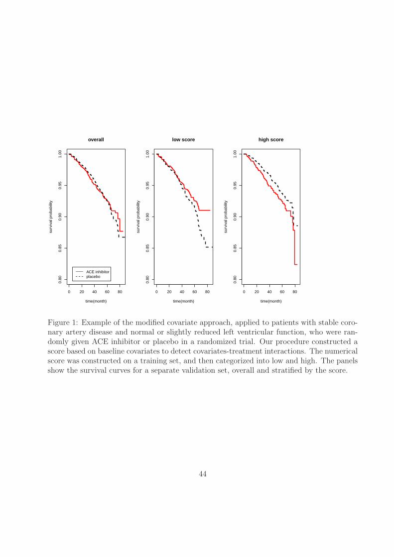
Figure 2 illustrates how the modified covariate method works for a single covariate Z
in two treatment groups. The raw data are shown on the left and the data with modified
covariate are shown on the right. The regression line computed in the right panel estimates
the treatment-covariate interaction.
The advantage of this new approach is twofold: it avoids having to directly model the
main effects and it has a causal interpretation for the resulting estimator regardless of the
adequacy of the assumed working model (3). Furthermore, unlike the modified outcome
method, it is straightforward to generalize the new approach to other types of outcome.
8

2.3 Binary Responses
When Y is a binary response, in the same spirit as the continuous outcome case, we propose
to fit a multivariate logistic regression model with modified covariates W∗ = W(Z) · T/2
generalized from (5):
Prob(Y = 1|Z, T ) =exp(γ ′0W
∗)1 + exp(γ ′0W∗)
. (7)
If model (7) is correctly specified, then
∆(z) = Prob(Y (1) = 1|Z = z)− Prob(Y (−1) = 1|Z = z)
= Prob(Y = 1|T = 1,Z = z)− Prob(Y = 1|T = −1,Z = z)
=exp{γ ′0W(z)/2} − 1
exp{γ ′0W(z)/2}+ 1,
and thus γ ′0W(z) has an appropriate causal interpretation. However, even when model (7) is
not correctly specified, we still can estimate γ0 by treating (7) as a working model. In general,
the maximum likelihood estimator (MLE) of the working model converges to a deterministic
limit γ∗ and W(z)′γ∗/2 can be viewed as the solution to the following optimization problem
maxfE{Y f(Z)T − log(1 + ef(Z)T )
}
subject to f ∈ F = {γ′W(z)/2|γ ∈ Rp},
where the expectation is with respect to (Y, T,Z). Therefore, if W(z) forms a “rich” set of ba-
sis functions, W(z)′γ∗/2 is an approximation to the minimizer of E{Y f(Z)T − log(1 + ef(Z)T )
}.
In the appendix 6.1, we show that the latter can be represented as
f ∗(z) = log
{1−∆(z)
1 + ∆(z)
}
9

under very general assumptions. Therefore,
∆(z) =exp{γ ′W(z)/2} − 1
exp{γ ′W(z)/2}+ 1
may serve as an estimate for the covariate-specific treatment effect and used to stratify the
patient population, regardless of the validity of the working model assumptions.
As described above, the MLE from the working model (7) can always be used to construct
a surrogate to the personalized treatment effect measured by the “risk difference”
∆(z) = E(Y (1) − Y (−1)|Z = z).
On the other hand, different measures for individualized treatment effects such as relative
risk may also be of interest. For example, if we consider an alternative approach for fitting
the logistic regression working model (7) by letting
γ = argminγ
N∑i=1
{(1− Yi)γ
′W∗ + Yie−γ′W∗
i
},
then γ converges to a deterministic limit γ∗ and exp{W(z)′γ∗(z)/2} can be viewed as an
approximation to
∆(z) =Prob(Y (1) = 1|Z = z)
Prob(Y (−1) = 1|Z = z),
which measures the treatment effect using “relative risk” rather than “risk difference”. This
loss function is motivated by the fact that the logistic regression model (7) can be fitted by
solving the estimating equation
N−1
N∑i=1
[W∗
i
{(1− Yi)− Yie
−γ′W∗i
}]= 0,
which is the derivative of the proposed loss function. The detailed justification is given in
10

appendix 6.1.
2.4 Survival Responses
When the outcome variable is survival time, we often do not observe the exact outcome for
every subject in a clinical study due to incomplete follow-up. In this case, we assume that
the outcome Y is a pair of random variables (X, δ) = {X ∧ C, I(X < C)}, where X is the
survival time of primary interest, C is the censoring time and δ is the censoring indicator.
Firstly, we propose to fit a Cox regression model with modified covariates
λ(t|Z, T ) = λ0(t)eγ′W∗
(8)
where λ(t|·) is the hazard function for survival time X and λ0(·) is a baseline hazard function
free of Z and T. When model (8) is correctly specified,
∆(z) =E{Λ0(X
(1))|Z = z}E{Λ0(X(−1))|Z = z}
=E{Λ0(X)|T = 1,Z = z}
E{Λ0(X)|T = −1,Z = z}= exp{−γ ′0W(z)}
and γ ′0W(z) can be used to stratify the patient population according to ∆(z), where Λ0(t) =∫ t
0λ0(u)du is a monotone increasing function (the baseline cumulative hazard function).
Under the proportional hazards assumption, the maximum partial likelihood estimator γ is
a consistent estimator for γ0 and semiparametric efficient. Moreover, even when model (8)
is mis-specified, we still can “estimate” γ0 by maximizing the partial likelihood function. In
general, the resulting estimator, γ, converges to a deterministic limit γ∗, which is the root
of a limiting score equation [Lin and Wei, 1989]. More generally, W(z)′γ∗/2 can be viewed
11

as the solution of the optimization problem
maxf
E
∫ τ
0
(f(Z)T − log[E{ef(Z)T I(X ≥ u)}]) dN(u)
subject to f ∈ F = {γ ′W(z)/2|γ ∈ Rp},
where N(t) = I(X ≤ t)δ, τ is a fixed time point such that Prob(X ≥ τ) > 0, and the expecta-
tions are with respect to (Y, T,Z). Therefore, W(z)′γ∗/2 can be viewed as an approximation
to
f ∗(z) = argmaxfE
∫ τ
0
(f(Z)T − log[E{ef(Z)T I(X ≥ u)}]) dN(u).
In appendix 6.1, we show that if the censoring time does not depend on (Z, T ), then the
minimizer f ∗ satisfies
ef∗(z)E{Λ∗(X(1))|Z = z} − e−f∗(z)E{Λ∗(X(−1))|Z = z}
=Prob(δ = 1|T = 1,Z = z)− Prob(δ = 1|T = −1,Z = z)
for a monotone increasing function Λ∗(u). Thus, when censoring rates are balanced between
the two arms, e.g., the hazard rate is low and most of the censoring is due to administrative
reasons,
f ∗(z) ≈ −1
2log
[E{Λ∗(X(1))|Z = z}E{Λ∗(X(−1))|Z = z}
]
can be used to characterize the covariate-specific treatment effect and stratify the patient
population even when the working model (8) is mis-specified.
2.5 Regularization for the High Dimensional Data
When the dimension of W∗, p, is high, we can easily apply appropriate variable selection
procedures based on the corresponding working model. For example, L1 penalized (Lasso)
12

estimators proposed by Tibshirani [1996] can be directly applied to the modified data (6).
In general, one may estimate γ by minimizing
1
N
N∑i=1
l(Yi,γ′W∗
i ) + λN‖γ‖1, (9)
where ‖γ‖1 =∑p
j=1 |γj| and
l(Yi, γ′W∗
i ) =
12(Yi − γ ′W∗
i )2 for continuous responses
−{Yiγ′W∗
i − log(1 + eγ′W∗i )} for binary responses
−[γ ′W∗
i − log{∑Nj=1 eγ′W∗
j I(Xj ≥ Xi)}]δi for survival responses
.
The resulting lasso regularized estimator may share the appealing finite sample oracle prop-
erties [Van De Geer, 2008, Zhang and Huang, 2008, Van De Geer and Buhlmann, 2009,
Negahban et al., 2012]. For example, for continuous outcomes, if we select the penalty
parameter λn = O({log(p)/N}1/2) and the covariates W(Zi)Ti/2, i = 1, · · · , N satisfy the
restricted eigenvalue condition, then
Prob
(‖γλN
− γ∗‖22 ≤ c3(#γ∗)
{log(p)
N
})≥ 1− c1e
−c2Nλ2N ,
where ‖γ‖22 =
∑pj=1 γ2
j , γλNis the corresponding lasso regularized estimator, #γ∗ is the
number of non-zero components in the vector γ∗, and ci, i = 1, 2, 3 are positive constants
depending on the joint distribution of (Y,W(Z), T ) [Negahban et al., 2012]. Therefore,
although the dimension p may be big, γ∗ can always be approximated by the lasso estimator
with an approximation error proportional to only the number of its non-zero components,
which is small if γ∗ is sparse. Following the Corollary 3 of Negahban et al. [2012], similar
results hold when γ∗ is not exactly sparse but can be approximated by a sparse vector. One
consequence is that if W(·) is adequately rich such that |γ∗W(z)− f ∗(z)| is small and γ∗ is
13

either exact or approximately sparse, then γ ′λNW(z) is a good approximation of f ∗(z) with a
high probability, where f ∗(z) is a monotone transformation of the individualized treatment
effect ∆(z). This property holds for any pair of finite N and p with a sufficiently small
ratio log(p)/N and does not depend on the correct specification of the working model. A
similar result for the expected utility in the patient population with the estimated optimal
treatment assignment rule has been established in Qian and Murphy [2011]. This result
can be extended to the binary case, with appropriate regularity condition on the covariates
W(Zi)Ti/2 to ensure that the negative log-likelihood function satisfies a form of restricted
strong convexity [Negahban et al., 2012]. For the survival case, parallel results have been
established for lasso-regularized maximum partial likelihood estimator under the assumption
that the multiplicative Cox model is correctly specified [Kong and Nan, 2012, Huang et al.,
2013]. The finite sample properties of the lasso estimator for mis-specified Cox model are
still unknown and warrants further study.
It might be reasonable to suppose that the covariates interacting with the treatment will
more likely be the ones exhibiting important main effects themselves. Therefore, one could
also apply the adaptive Lasso procedure [Zou, 2006] with feature weights wj proportional to
the reciprocal of the univariate “association strength” between the outcome Y and the jth
component of W(Z). Specifically, one may modify the penalty in (9) as
λN
p∑j=1
|γj|wj
, (10)
where wj = |θi|−1 or (|θ−1i| + |θ1i|)−1. Here θj1, θj(−1) and θj, are the estimated regression
coefficients of the jth component of W(Z) in appropriate univariate regression analysis with
observations from the group T = 1, the group T = −1, and the combined group, respectively.
Other regularization methods such as elastic net may also be used [Zou and Hastie, 2005].
Interestingly, one can treat the modified data (6) just as generic data and hence couple
14

it with other statistical learning techniques. For example, one can apply a classifier such
as prediction analysis of microarrays (PAM) to the modified data for the purpose of finding
subgroup of samples in which the treatment effect is large. We can also do large scale
hypothesis testings on the modified data to determine which gene-treatment interactions
have significant effects on the outcome.
2.6 Efficiency Augmentation
When the models (5, 7 and 8) with modified covariates are correctly specified, the MLE
estimator for γ∗ is the most efficient estimator asymptotically. However, when models are
treated as working models subject to mis-specification, a more efficient estimator can be
obtained for estimating the same γ∗. To this end, note that in general γ is defined as the
minimizer of an objective function motivated from a working model:
γ = argminγ
1
N
N∑i=1
l(Yi,γ′W∗
i ). (11)
Since for any function a(z) : Rq → Rp, E{Tia(Zi)} = 0 due to randomization, the minimizer
of the augmented objective function
1
N
N∑i=1
{l(Yi,γ′W∗
i )− Tia(Zi)′γ}
converges to the same limit as γ. Furthermore, by selecting an optimal augmentation term
a(·), the minimizer of the augmented objective function may have smaller variance than that
of the minimizer of the original objective function. In appendix 6.2, we show that
a0(z) = −1
2W(z)E(Y |Z = z) and a0(z) = −1
2W(z){E(Y |Z = z)− 0.5}
15

are optimal choices for continuous and binary responses, respectively. Therefore, we propose
the following two-step procedures for estimating γ∗ :
16

1. Estimate the optimal a0(z) :
(a) For continuous responses, fit the linear regression model E(Y |Z) = ξ′B(Z) for the
appropriate function B(Z) with OLS. Appropriate regularization will be used if
the dimension of B(Z) is high. Let
a(z) = −1
2W(z)× ξ′B(z).
(b) For binary response, fit the logistic regression model logit{Prob(Y = 1|Z)} =
ξ′B(Z) for the appropriate function B(Z) by maximizing the likelihood function.
Let
a(z) = −1
2W(z)×
{eξ′B(z)
1 + eξ′B(z)− 1
2
}.
Here B(z) = {B1(z), · · · , BS(z)} and {Bs(z) : Rq → R1, 1 ≤ s ≤ S} is a set of basis
functions selected by users for capturing the relationship between Y and Z. It may
include, for example, spline basis functions, interactions or other transformations of
the original covariates. In practice, B(z) is not necessarily but can be the same as
W(z).
2. Estimate γ∗
(a) For continuous responses, we minimize
1
N
N∑i=1
{1
2(Yi − γ ′W∗
i )2 − γ ′a(Zi)Ti
}.
(b) For binary responses, we minimize
1
N
N∑i=1
[−{Yiγ
′W∗i − log(1 + eγ′W∗
i )} − γ ′a(Zi)Ti
].
17

For survival outcome, the log-partial likelihood function is not a simple sum of i.i.d terms.
However, in appendix 6.2, we show that the optimal choice of a(z) is
a0(z) = −1
2
[1
2W(z) {G1(τ ; z) + G2(τ ; z)} −
∫ τ
0
R(u; γ∗){G1(du; z)−G2(du; z)}]
,
where G1(u; z) = E{M(u)|Z = z, T = 1}, G2(u; z) = E{M(u)|Z = z, T = −1},
M(t,W∗,γ) = N(t)−∫ t
0
I(X ≥ u)eγ′W∗dE{N(u)}
E{eγ′W∗I(X ≥ u)}
and
R(u; γ) =E{W∗eγ′W∗
I(X ≥ u)}E{eγ′W∗I(X ≥ u)} .
Unfortunately, a0(z) depends on the unknown parameter γ∗. On the other hand, for the
high-dimensional case, the interaction effect is usually small and it is not unreasonable to
assume that γ∗ ≈ 0. Furthermore, if the censoring patterns are similar in both arms, we
have G1(u, z) ≈ G2(u, z). Using these two approximations, we can simplify the optimal
augmentation term as
a0(z) = −1
4W(z) {G1(τ ; z) + G2(τ ; z)} = −1
2W(z)× E{M(τ)|Z = z)
where
M(t) = N(t)−∫ t
0
I(X ≥ u)dE{N(u)}E{I(X ≥ u)} .
Therefore, we propose to employ the following approach to implement the efficiency aug-
mentation procedure:
18

1. Calculate
Mi(τ) = Ni(τ)−∫ τ
0
I(Xi ≥ u)d{∑Nj=1 Nj(u)}
∑Nj=1 I(Xj ≥ u)
for i = 1, · · · , N and fit the linear regression model E(M(t)|Z) = ξ′B(Z) for the
appropriate function B(Z) with OLS and appropriate regularization if needed. Let
a(z) = −1
2W(z)× ξ′B(z).
2. Estimate γ∗ by minimizing
1
N
N∑i=1
(−
[γ ′W∗
i − log{N∑
j=1
eγ′W∗i I(Xj ≥ Xi)}
]∆i − γ ′a(Zi)Ti
)
with appropriate penalization if needed.
Remark 1
When the response is continuous, the efficient augmentation estimator is the minimizer
of
N∑i=1
[1
2
{Yi − 1
2γ ′W(Zi)Ti/2
}2
− γ ′a(Zi)Ti
]
=N∑
i=1
1
2
{Yi − ξ′B(Zi)− 1
2γ ′W(Zi)Ti
}2
+ constant.
This equivalence implies that this efficiency augmentation procedures is asymptotically
equivalent to that based on a simple multivariate regression with main effect ξ′B(Z) and
interaction γ ′W(Z) · T. This is not a surprise. As we pointed out in section 2.1, the choice
of the main effect in the linear regression does not affect the asymptotical consistency of
19

estimating the interactions. On the other hand, a good choice of main effect model can help
estimate the interaction, i.e., personalized treatment effect, more accurately.
Another consequence is that one may directly use the same standard algorithm to obtain
the augmented estimator when the lasso penalty is used. For binary or survival responses, the
augmented estimator under the lasso regularization can be obtained with slightly modified
algorithm designed for the lasso optimization as well. The detailed algorithm is given in
appendix 6.3.
Remarks 2
For nonlinear models such as logistic and Cox regressions, the augmentation method is
NOT equivalent to the full regression approach including both the main effect and interac-
tion terms. In those cases, different specifications of the main effects in the full regression
model result in asymptotically different estimates for the interaction terms, which, unlike
the proposed modified covariate estimators, in general can not be interpreted as surrogates
for the personalized treatment effects.
Remark 3
With binary responses, the estimating equation targeting on approximating the relative
risk is
N−1
N∑i=1
W∗i {(1− Yi)− Yie
−γ′W∗i } = 0
and the optimal augmentation term a0(z) can be approximated by
−1
2W(z)
{E(Y |Z = z)− 1
2
}
20

when γ∗ ≈ 0. The efficiency augmentation algorithm can be carried out accordingly.
Remark 4
The similar technique can also be used for improving other estimators such as that
proposed by Zhao et al. [2012], where the surrogate objective function for the weighted mis-
classification error can be written in the form of (2.6) as well. The optimal function a0(z)
needs to be derived case by case.
3 Numerical Studies
In this section, we perform extensive numerical studies to investigate the finite sample per-
formance of the proposed method in various settings: the treatment may or may not have
the marginal main effect; the personalized treatment effect may depend on complicated func-
tions of covariates such as interactions among covariates; the regression model for detecting
the interactions may or may not be correctly specified. Due to the limitation of the space,
we only present simulation results from the selected representative cases. The results for
other scenarios are similar to those presented.
3.1 Continuous Responses
For continuous responses, we generated N independent Gaussian samples from the regression
model
Y = (β0 +
p∑j=1
βjZj)2 + (γ0 +
p∑j=1
γjZj +∑
1≤i<j≤p
αijZiZj)T + σ0 · ε, (12)
21

where the covariates (Z1, · · · , Zp) follow a mean zero multivariate normal distribution with
a compound symmetric variance-covariance matrix, (1−ρ)Ip +ρ1′1, and ε ∼ N(0, 1). We let
(γ0, γ1, γ2, γ3, γ4, γ5, · · · , γp) = (0.4, 0.8,−0.8, 0.8,−0.8, 0, · · · , 0), αij = 0.8I(i = 1, j = 2),
σ0 =√
2, N = 100, and p = 50 and 1000 representing high and low dimensional cases,
respectively. The treatment T was generated as ±1 with equal probability at random. We
consider four sets of simulations:
1. β0 = (√
6)−1, βj = (2√
6)−1, j = 3, 4, · · · , 10 and ρ = 0;
2. β0 = (√
6)−1, βj = (2√
6)−1, j = 3, 4, · · · , 10 and ρ = 1/3;
3. β0 = (√
3)−1, βj = (2√
3)−1, j = 3, 4, · · · , 10 and ρ = 0;
4. β0 = (√
3)−1, βj = (2√
3)−1, j = 3, 4, · · · , 10 and ρ = 1/3.
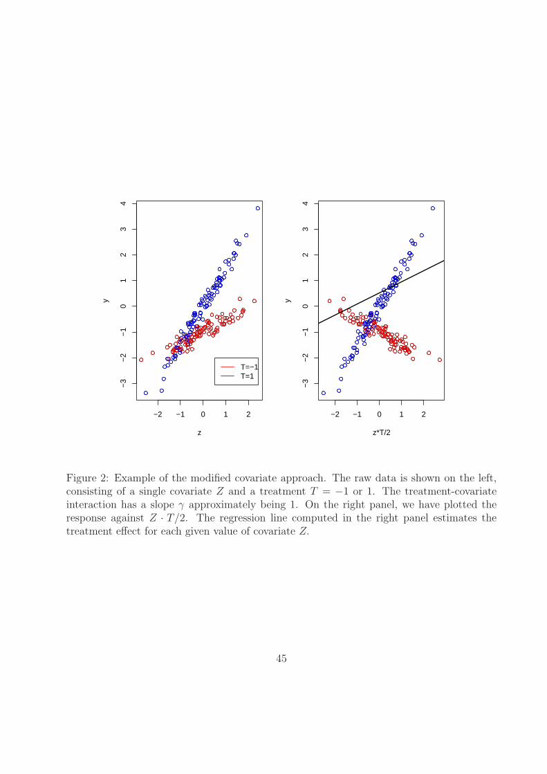
Settings 1 and 2 represented cases with relatively small main effects, where the variances in
response contributable to the main effect, interaction and random error were about 37.5%,
37.5% and 25%, respectively, when the covariates were correlated. Settings 3 and 4 repre-
sented cases with relatively big main effects, where the variances in response contributable
to the main effect, interaction and random error were about 75%, 15% and 10%, respectively,
when the covariates were correlated. For each of the simulated data set, we implemented
three methods:
• full regression: Fit a multivariate linear regression with complete main effects and
covariate/treatment interaction terms, i.e., the dimension of the covariate matrix was
2(p + 1). The Lasso was used to select the variables.
• new: Fit a multivariate linear regression with the modified covariate W∗ = (1,Z)′ ·T/2.
The dimension of the covariate matrix was p+1. Again, the Lasso was used for selecting
variables.
22

• new/augmented: The proposed method with efficiency augmentation, where E(Y |Z)
was estimated with lasso-regularized ordinary least squared method and B(z) = z.
The selection of W(z) = B(z) = z mimicked the realistic situation where the knowledge of
the true functional forms for interaction and main effects were often lacking. For all three
methods, we selected the Lasso penalty parameter via 20-fold cross-validation. To evaluate
the performance of the resulting score measuring the individualized treatment effect, we
estimated the Spearman’s rank correlation coefficient between the estimated score and the
“true” treatment effect
∆(Z) = E(Y (1) − Y (−1)|Z) = 1.6× (0.5 + Z1 − Z2 + Z3 − Z4 + Z1Z2)
in an independently generated set with a sample size of 10000. Based on 500 sets of sim-
ulations, we plotted the boxplots of the rank correlation coefficients between the estimated
scores γ ′Z and ∆(Z) under simulation settings (1), (2), (3) and (4) in the top left, top
right, bottom left and bottom right panels of Figure 3, respectively. For the first three set-
tings, the performance of the proposed method was better than that of the full regression
approach. The superiority of the new method was fairly obvious especially when p = 1000.
For example, in the setting 3, where all the covariates were independent and the main ef-
fect was relatively big, the median correlation coefficients were 0.14, 0.51 and 0.51 for the
full regression, new and new/augmented methods, respectively. In the setting 4, the most
challenging setting to estimate the individualized treatment effect, the median correlation
coefficients were zero for all the methods. On the other hand, the proportions of obtaining
a positive correlation coefficient are 41%, 48% and 46% for the full regression, new and
new/augmented methods, respectively, while the corresponding proportions of obtaining a
negative correlation coefficient, which corresponded to a false detection, were 34%, 20% and
17%, respectively. Therefore, the proposed method with and without augmentation was still
23

superior to the conventional counterpart. Furthermore, the new method was also superior
in terms of selecting the right covariates interacting with the treatment. For example, in
the setting 3 with p = 1000, while the proposed method (with or without augmentation)
on average selected 8 covariates with 2 true positives, i.e. covariates from Zi, 1 ≤ i ≤ 4,
the full regression method only selected 5 covariates with one true positive. If p reduced
to 50, then on average, the proposed method (with or without augmentation) selected 9.5
covariates with 4 true positives and the full regression method selected 11.5 covariates with
3 true positive.
3.2 Binary Responses
For binary responses, we used the same simulation design as that for the continuous response.
Specifically, we generated N independent binary samples from the regression model
Y = I
((β0 +
p∑j=1
βjZj)2 + (γ0 +
p∑j=1
γjZj +∑
1≤i<j≤p
αijZiZj)T + σ0 · ε ≥ 0
), (13)
where all the model parameters were the same as those in the case of continuous responses.
Noting that the logistic regression model was mis-specified under the chosen simulation
design. We also considered the same four settings with different combinations of βj and ρ.
For each of the simulated data set, we implemented three methods:
1. full regression: Fit a lasso regularized multivariate logistic regression with complete
main effects and covariate/treatment interaction terms.
2. new: Fit a lasso regularized multivariate logistic regression (without intercept) with
the modified covariate W∗ = (1,Z)′ · T/2.
3. new/augmented: The proposed method with efficiency augmentation, where E(Y |Z)
was estimated with Lasso-penalized logistic regression.
24

To evaluate the performance of the resulting score measuring the individualized treatment
effect, we estimated the Spearman’s rank correlation coefficient between the estimated score
and the “true” treatment effect
∆(Z) = E(Y (1) − Y (−1)|Z)
Although the scores measuring the interaction from the first and second/third methods were
different even when the sample size goes to infinity, the rank correlation coefficients put them
on the same footing in comparing performances.
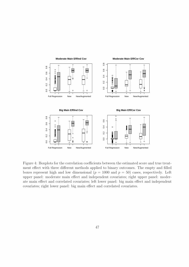
In the top left, top right, bottom left and bottom right panels of Figure 4, we plotted the
boxplots of the correlation coefficients between the estimated scores γ ′Z and ∆(Z) under
simulation settings (1), (2), (3) and (4), respectively. The patterns were similar to that for
the continuous response. The “new/augmented method” performed the best or close to the
best in all four settings. For example, in the setting 3, the median correlation coefficients were
0.02, 0.15 and 0.17 for the full regression, new and new/augmented methods, respectively,
when p = 1000. In addition, while the proposed methods on average selected 15 covariates
with 2 true positives, the full regression method only selected 2 covariates with 0.3 true
positive in the same setting.
3.3 Survival Responses
For survival responses, we used the same simulation design as that for the continuous and
binary responses. Specifically, we generated N independent survival time from the regression
model
X = exp
{(β0 +
p∑j=1
βjZj)2 + (γ0 +
p∑j=1
γjZj +∑
1≤i<j≤p
αijZiZj)T + σ0 · ε}
, (14)
25

where all the model parameters were the same as in the previous subsections. The censoring
time was generated from the uniform distribution U(0, ξ0), where ξ0 was selected to induce
a censoring rate of 25%. For each simulated data set, we implemented the following three
methods:
1. full regression: Fit a lasso regularized multivariate Cox regression with full main effect
and covariate/treatment interaction terms, i.e., the dimension of the covariate matrix
was 2p + 1.
2. new: Fit a lasso regularized multivariate Cox regression with modified covariates.
3. new/augmented: The proposed method with efficiency augmentation. To model the
E{M(τ)|Z}, we used linear regression with the lasso regularization method.
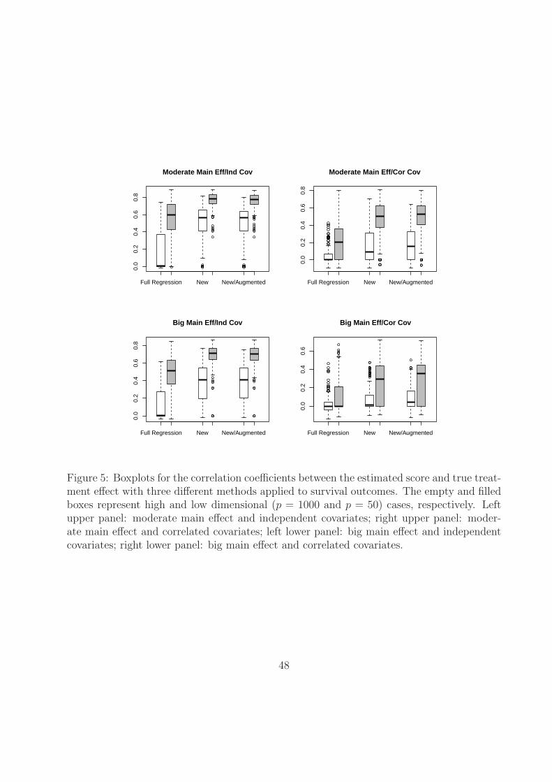
To evaluate the performance of the resulting score measuring the individualized treatment
effect, we estimated the Spearman’s rank correlation coefficient between the estimated score
and the “true” treatment effect based on survival probability at t0 = 20
∆(Z) = Prob(X(1) ≥ t0|Z)− Prob(X(−1) ≥ t0|Z)
In the top left, top right, bottom left and bottom right panels of Figure 5, we plotted the
boxplots of the correlation coefficients between the estimated scores γ ′Z and ∆(Z) under
simulation settings, (1), (2), (3) and (4), respectively. The patterns were similar to those
for the continuous and binary responses and confirmed our findings that the “efficiency-
augmented method” performed the best among the three methods. For example, when
p = 1000, the median correlation coefficients were 0.00, 0.41 and 0.41 in the setting 3 for
the full regression, new and new/augmented methods, respectively. In addition, on average
the proposed method selected 11 covariates with 2.2 true positives and the full regression
method only selected 2 covariates with 0.5 true positive in the same setting.
26
4 Examples
In this section, we applied the proposed method to analyze two real data examples. In the
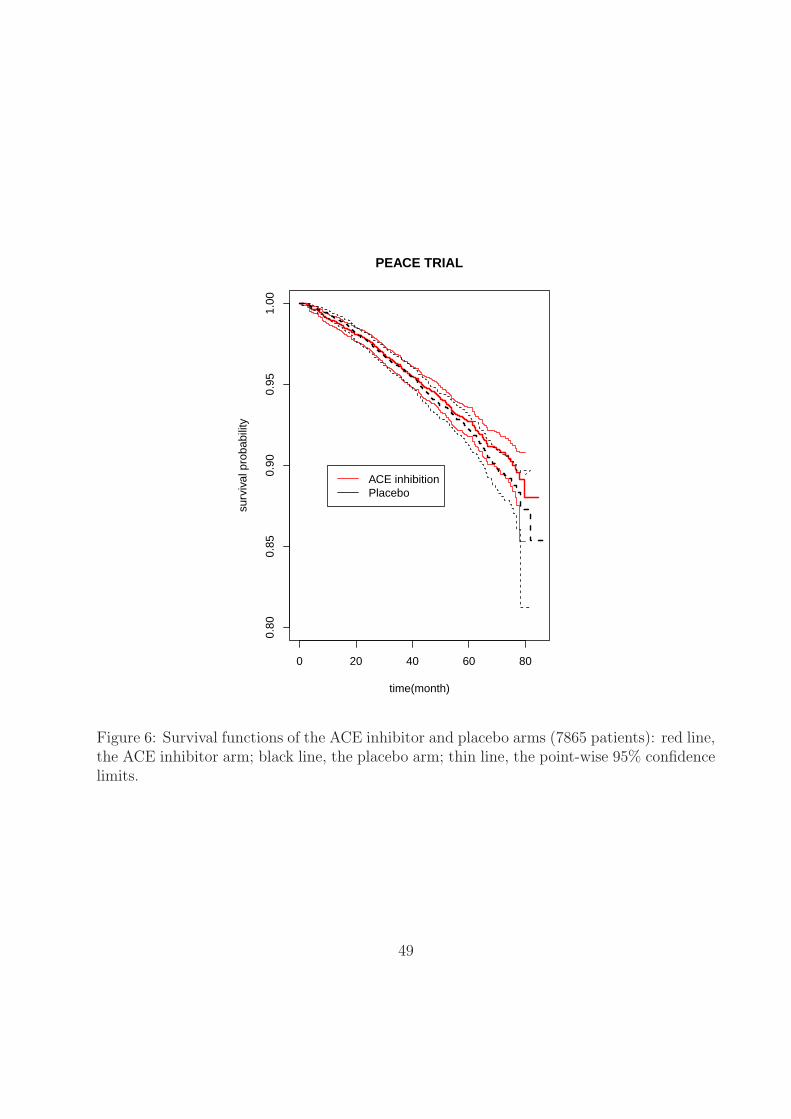
first example, we considered a recent clinical trial “Preventive of Events with Angiotensin
Converting Enzyme Inhibition” (PEACE) to study if the ACE inhibitors are effective for
lowering cardiovascular risk for patients with stable coronary artery disease and normal
or slightly reduced left ventricular function [Braunwald et al., 2004]. In this study, 8290
patients were randomly assigned to treatment and control arms with 633 deaths occurred by
the end of the study. The estimated hazard ratio is 0.95 with an insignificant p-value of 0.13.
However, in a secondary analysis, Solomon et al. [2006] reported that ACE inhibitors might
significantly reduce the mortality for patients whose kidney function was abnormal at the
baseline. Although this result needs to be interpreted cautiously, it suggests the possibility
of existence of a subgroup of patients who may benefit from the treatment. For this example,
we considered the survival time as the primary endpoint and the objective was to use seven
baseline covariates: age, gender, left ventricular ejection fraction (LVEF), renal function
measured by EGFR, hypertension, diabetic status and history of myocardial infarction to
build a scoring system capturing the individualized treatment effect. Those covariates were
selected for their known association with the cardiovascular risk. The continuous covariates,
age, LVEF and EGFR are log-transformed. In addition to the seven covariates, we also
included all the two-way interactions among them in the model. In summary, Z was a 7
dimensional vector and W(Z) was a 7 + 7 × 6/2 = 28 dimensional vector. We included all
patients with complete information on these seven covariates. The final data set consisted
of 3947 patients in the treatment arm and 3918 patients in the placebo arm. The outcome
of interest was the survival time and there were 292 and 315 deaths in the treatment and
placebo arms, respectively. The estimated survival curves by arms were plotted in figure
6. The goal of the analysis was to construct a score using baseline covariates to identify
27

subgroups of patients who may or may not be benefited from the ACE inhibition treatment.
To this end, we selected the first 2000 patients in the treatment arm and placebo arm to
form the training set and reserved the rest 3865 patients as an independent validation set.
In selecting the training and validation sets, we used the original order of the observations
in the data set without additional sorting to ensure the objectivity.
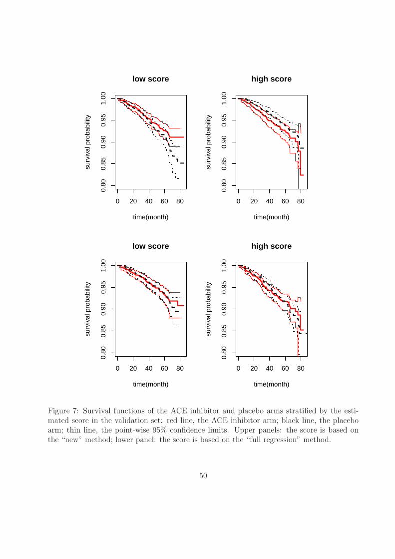
First we maximized the partial likelihood function with modified covariates to construct
a score aiming for capturing the individualized treatment effect. The resulting score was a
linear combination of selected covariates and their two-way interactions. Here, a low score
favored ACE inhibition treatment. We then applied the score to classify the patients in the
validation set into the high and low score groups depending on whether the patient’s score
was greater than the median level. In the high score group, the survival time in the ACE
inhibition arm was slightly shorter than that in the placebo arm with an estimated hazard
ratio of 1.27 for ACE inhibitor versus placebo (p = 0.163). In the low score group, the survival
time in the ACE inhibition arm was longer than that in the placebo arm with an estimated
hazard ratio of 0.74 (p = 0.061). The estimated survival functions of both treatment arms
were plotted in the upper panels of Figure 7. The interaction between the constructed score
and treatment was statistically significant in the multivariate Cox regression based on the
validation set (p = 0.022).
Furthermore, we implemented the efficiency augmentation method and obtained a new
score. Again, we classified the patients in the validation set into the high and low score
groups based on the constructed gene score. The results were very similar and the interaction
between the constructed score and treatment was also statistically significant (p = 0.025).
For comparison purposes, we also fitted a multivariate Cox regression model with treat-
ment, W(Z), and their interactions as the covariates. In this model, we had 57 different
covariates. The resulting score failed to stratify the population according to the treatment
effect in the validation set. The results were shown in the lower panel of Figure 7. The
28

interaction between the constructed score and treatment was not statistically significant
(p = 0.980).
To further objectively examine the performance of the proposal in this data set, we
randomly split the data into a training set of 2000 patients and a validation set of 5865
patients. We then estimated the score measuring individualized treatment effect in the
training set with the modified covariates and full regression approaches. The lasso method
coupled with BIC criterion was used in the full regression approach due to the large number
of covariates relative to the number of deaths in the training set. Patients in the validation
set were then stratified into the high and low score groups. We calculated the hazard
ratios of the ACE inhibition arm versus the placebo arm in high and low score groups,
respectively. In Figure 8, we plotted the boxplots of the hazard ratios in the high and low
risk groups of the validation set based on 500 random splits. The results indicated that the
proposed method tended to perform better than the commonly used full regression method
in separating patients according to the treatment effect measured by the hazard ratio, which
was consistent with our previous findings from the simulation studies. Furthermore, the
empirical probability of obtaining an interaction significant at the one-sided 0.05 level in the
validation set was 27.0% for the new method and 13.6% for the full regression method. This
observation supported that our previous significant findings for the detected interaction was
likely not due to the random chance.
It has been known that the breast cancer can be classified into different subtypes us-
ing gene expression profile and the effective treatment may be different for different sub-
types of the disease [Loi et al., 2007]. In the second example, we applied the proposed
method to study the potential interactions between gene expression levels and Tamoxifen
treatment in breast cancer patients. The data set consisted of 414 patients in the co-
hort GSE6532 collected by Loi et al. [2007] for the purpose of characterizing ER-positive
subtypes with gene expression profiles. The data set can be downloaded from the web-
29

site www.ncbi.nlm.nih.gov/geo/query/acc.cgi?acc=GSE6532. Excluding patients with in-
complete information, there were 268 and 125 patients receiving Tamoxifen and alternative
treatments, respectively. In addition to the routine demographic information, we had 44, 928
gene expression measurements for each of the 393 patients. The outcome of the primary in-
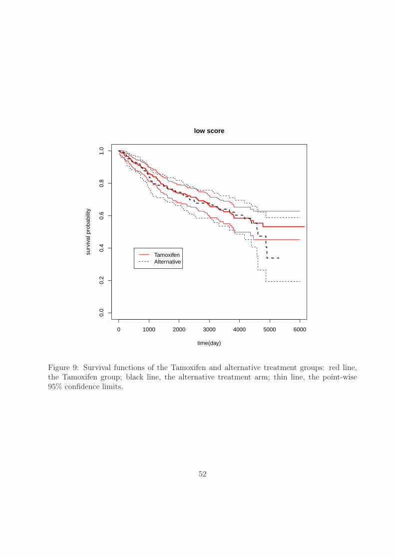
terest here was the distant metastasis free survival (MFS) time, which could be right censored
due to incomplete follow-up. The MFS times were not statistically different between the two
groups with a two-sided p value of 0.59 (Figure 9). The goal of the analysis was to construct
a gene score using gene expression levels to identify a subgroup of patients who may benefit
from the Tamoxifen treatment. We selected the first 90 patients from each group to form
the training set and reserved the rest 213 patients as the independent validation set.
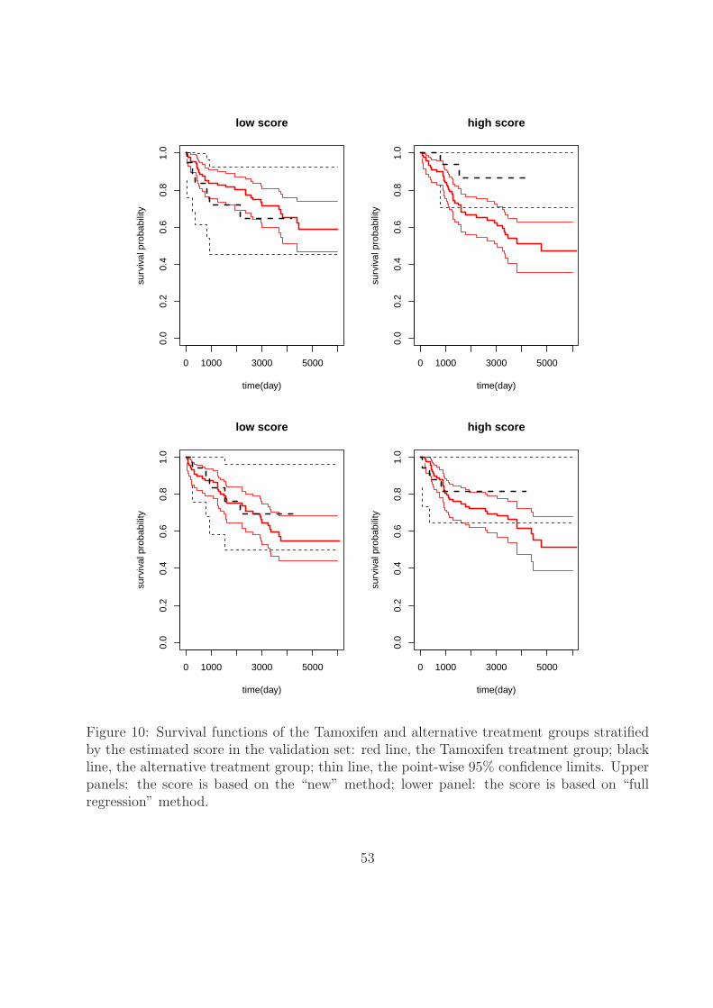
We identified 5,000 genes with the highest empirical variances and then constructed a
gene score by fitting the Lasso penalized Cox regression model with modified covariates
in the training set. The Lasso penalty parameter was selected via cross-validation. The
resulting gene score was a linear combination of expression levels of seven genes. We applied
the gene score to classify the patients in the validation set into the high and low score
groups according to the median. In the high score group, the MFS time in the Tamoxifen
group was shorter than that in the alternative group with an estimated hazard ratio of 3.52
(p = 0.064). In the low score group, the MFS time in the Tamoxifen group was longer than
that in the alternative group with an estimated hazard ratio of 0.694 (p = 0.421). The
estimated survival curves for both groups were plotted in the upper panels of Figure 10.
The interaction between constructed score and treatment was statistically significant in the
validation set (p = 0.004).
We implemented the efficiency augmentation method to obtain a new gene score, which
was based on the expression level of eight genes. Again, we classified the patients in the
validation set into the high and low score groups using the constructed score. The results
were very similar to that from the gene score constructed without augmentation.
30

When we fitted a multivariate Cox regression model with treatment, the gene expression
levels, and all treatment-gene interactions as the covariates, only one gene interacting with
the treatment was selected by lasso. However, the interaction could not be reproduced in
the validation set (lower panel of Figure 10). Furthermore, the computational speed was
substantially slower due to the high-dimensional covariates matrix in this case.
The second example was chosen for demonstrating the potential use of the proposed
method in the high-dimensional setting. An important limitation of this example is that the
treatment was not randomly assigned to patients as in a standard randomized clinical trial
and the gene expression levels were measured at the study baseline, which may be different
from treatment initiation time. Therefore, the results need to be interpreted with caution
and further verification based on data from a randomized clinical trial is desired.
5 Discussion
In this paper, we have proposed a simple method to explore the potential interactions between
treatment and a set of high dimensional covariates. The general idea is to use W(Z) · T/2
as new covariates in a regression model to predict the outcome. This provides a conve-
nient approach for constructing a proper objective function whose optimizer can be used
to estimate the individualized treatment effect as a function of given covariates. Once the
objective function is constructed, one may employ one’s favorite algorithms such as lasso
and boosting to optimize the empirical version of the objective function and the resulting
estimator can be used to stratify the patient population according to the treatment benefit.
Therefore, the proposed method can be used in a much broader way than those already
described in the paper. For example, after creating the modified covariates W(Z) ·T/2, data
mining techniques such as nearest shrunken centroid classification, PAM and support vector
machines can also be used to link the new covariates with the outcomes [Friedman, 1991,
31

Tibshirani et al., 2003, Hastie and Zhu, 2006]. Most dimension reduction methods in the
literature can be readily adapted to handle the potentially high dimensional covariates. For
univariate analysis, we also may perform large scale hypothesis testing on the modified data,
to identify a list of covariates having interaction with the treatment; one could for example
directly use the Significance Analysis of Microarrays (SAM) method [Gilbert et al., 2002] for
this purpose. Extensions in these directions are promising and warrant further research.
As a limitation, the proposed method is primarily designed for analyzing data from ran-
domized clinical trials. When applied to an observational study, where the covariates and
treatment assignment are correlated, the constructed score may lose its causal interpretation.
On the other hand, if a reasonable propensity score model is available, then we can still im-
plement the modified covariate approach on matched or reweighted data so that the resulted
score may retain the appropriate causal interpretations [Rosenbaum and Rubin, 1983].
Lastly, we want to emphasize that although the proposed method aims to estimate the
individualized treatment effect with casual interpretation, the method is not immune to
the common problems encountered in high dimensional data analysis such as multiple test-
ing, false discovery, over-fitting et al., as the numerical studies demonstrated. To reinforce
this point, we have repeated the simulation studies in Section 3 after removing the co-
variate/treatment interaction in generating the observed data and have found that there
is non-negligible probability of false discoveries albeit the employment of cross-validation.
In a typical example, where the covariates are independent and p = 50, the probabilities of
detecting a non-existent interactions are as high as 52%, 44% and 40% for the full regression,
new and new/augmented methods, respectively. Therefore the proposed method is just an
exploratory tool and it is crucial to withhold an independent validation set, which can be
used to verify the detected interaction. In the validation set, one may make valid statis-
tical inference on various parameters of interest. For example, one may estimate and test
the treatment effect in subgroup of patients selected from the detected covaraite/treatment
32
interactions and the results will have causal interpretation if the validation set is from a
randomized clinical trial.
References
M. Bonetti and R. Gelber. Patterns of treatment effects in subsets of patients in clinical
trials. Biostatistics, 5(3):465–81, 2004.
E Braunwald, M Domanski, S Fowler, N Geller, B Gersh, J Hsia, M Pfeffer, M Rice, Y Rosen-
berg, J Rouleau, and PEACE trial investigators. Angiotension-coverting-enzyme inhibition
in stable coronary artery disease. New England Journal of Medicine, 351:2058–2068, 2004.
W. Chen, D. Ghosh, T. Raghunathan, M. Norkin, D. Sargent, and G. Bepler. On
bayesian methods of exploring qualitative interactions for targeted treatment. Statistics
in Medicine, 31, 2012.
H. Chipman, E. George, and R. McCulloch. Bayesian cart model search. Journal of the
American Statistical Association, 93, 1998.
J. Friedman. Multivariate adaptive regression splines (with discussion). Annals of Statistics,
19(1):1–141, 1991.
C. Gilbert, B. Narasimhan, R. Tibshirani, and V. Tusher. Significance analysis of microar-
rays (sam) software. 2002. Available: http://www-stat.stanford.edu/˜tibs/SAM/ via the
Internet. Accessed 2003 July 16.
P. Gustafson. Bayesian regression modeling with interactions and smooth effects. Journal
of the American Statistical Association, 95(451):795–806, 2000.
T. Hastie and J. Zhu. Discussion of ”support vector machines with applications” by Javier
Moguerza and Alberto Munoz. Statistical Science, 21(3):352–357, 2006.
33

J Huang, T Sun, Z Ying, and C Zhang. Oracle inequalities for the lasso in the cox model.
Annals of Statistics, 41:1055–1692, 2013.
S Kong and B Nan. Non-asymptotic oracle inequalities for the high-dimensional cox regres-
sion via lasso. Tech Report, page 1204.1992, 2012.
M. LeBlanc. An adaptive expansion method for regression. Statistical Sinica, 5, 1995.
D. Lin and LJ. Wei. Robust inference for the cox proportional hazards model. Journal of
the American Statistical Association, 84(107):1074–1078, 1989.
S. Loi, B. Haibe-kains, C. Desmedt, and et al. Definition of clinically distinct molecular
subtypes in estrogen rceptor-positive breast carcinomas through genomic grade. Journal
of Clinical Oncology, 25(10):1239–1246, 2007.
S. Negahban, P. Ravikumar, M. Wainwright, and B. Yu. A unified framework for high
dimensional analysis of m-estimators with decomposable regularizers. Statistical Science,
27:1214/12–STS400, 2012.
M Qian and S Murphy. Performance guarantees for individualized treatment rules. Annals
of Statistics, 39:1180–1210, 2011.
P. Rosenbaum and D. Rubin. The central role of the propensity score in observational studies
for causal effects. Biometrika, 70:41–55, 1983.
P. Royston and W. Sauerbrei. Interactions between treatment and continuous covariates: A
step toward individualizing therapy. Journal of Clinical Oncology, 26(9):1397–99, 2008.
W. Sauerbrei, P. Royston, and K. Zapien. Detecting an interaction between treatment and
a continuous covariate: A comparison of two approaches. Computational Statistics and
Data Analysis, 51(8):4054–63, 2007.
34

S Solomon, M Rice, K Jablonski, J Jose, M Domanski, M Sabatine, B Gersh, J Rouleau,
M Pfeffer, E Braunwald, and (PEACE) Investigators. Renal function and effectiveness of
angiotensin-converting enzyme inhibitor therapy in patients with chronic stable coronary
disease in the prevention of events with ace inhibition (peace) trial. Circulation, 114:26–31,
2006.
X. Su, T. Zhou, X. Yan, F. Fan, and S. Yang. Interaction trees with censored survival data.
The International Journal of Biostatistics, 4(1):Article 2, 2008.
L. Tian and R. Tibshirani. Adaptive index models for marker-based risk stratification.
Biostatistics, page 10.1093/biostatistics/kxq047, 2010.
R. Tibshirani. Regression shrinkage and selection via the lasso. Journal of the Royal Statis-
tical Society, Series B, 58:267–288, 1996.
R. Tibshirani, T. Hastie, B. Narasimhan, and C. Gilbert. Prediction analysis for microarrays
(pam) software. 2003. /home/tibs/publichtml/PAM .
S. Van De Geer. High-dimensional gneralized linear models and lasso. Annals of Statistics,
36:614–645, 2008.
S. Van De Geer and P Buhlmann. On the conditions used to prove oracle results for lasso.
Electronic Journal of Statistics, 3:1360–1392, 2009.
C. Zhang and J Huang. The sparsity and bias of the lasso selection in high-dimensional
linear regression. Annals of Statistics, 36:1567–1594, 2008.
Y. Zhao, D. Zeng, A. Rush, and M. Kosorok. Estimating individualized treatement rules
using outcome weighted learning. Journal of the American Statistical Association, 107
(499):1106–1118, 2012.
35

H. Zou. The adaptive lasso and its oracle properties. Journal of the American Statistical
Association, 101:1418–1429, 2006.
H. Zou and T. Hastie. Regularization and variable selection via elastic net. Journal of Royal
Statistical Socienty. B, 67:301–320, 2005.
6 Appendix
6.1 Justification of the Objective Function Based on the Working
Model
Under the linear working model for continuous responses, we have
E{l(Y, f(Z)T )|Z, T = 1} =1
2
[E{(Y (1))2|Z} − 2m1(Z)f(Z) + f(Z)2
]
and
E{l(Y, f(Z)T )|Z, T = −1} =1
2
[E{(Y (−1))2|Z}+ 2m−1(Z)f(Z) + f(Z)2
],
where mt(z) = E(Y (t)|Z = z) for t = 1 and -1. Therefore
L(f) =E{l(Y, f(Z)T )}
=EZ
[1
2EY {l(Y, f(Z)T )|Z, T = 1}+
1
2EY {l(Y, f(Z)T )|Z, T = −1}
]
=EZ
([1
2{m1(Z)−m−1(Z)} − f(Z)
]2)
+ constant.
The minimizer of this objective function is
f ∗(z) =1
2{m1(z)−m−1(z)} =
1
2∆(z)
36

for all z ∈ Support of Z.
Under the logistic working model for binary responses, we have
E{l(Y, f(Z)T )|Z, T = 1} = m1(Z)f(Z)− log(1 + ef(Z)),
and
E{l(Y, f(Z)T )|Z, T = −1} = −m−1(Z)f(Z)− log(1 + e−f(Z)).
Thus
L(f) =E{l(Y, f(Z)T )}
=EZ
[1
2EY {l(Y, f(Z)T )|Z, T = 1}+
1
2EY {l(Y, f(Z)T )|Z, T = −1}
]
=1
2EZ
[∆(Z)f(Z)− log(1 + ef(Z))− log(1 + e−f(Z))
].
Therefore
∂L(f)
∂f=
1
2EZ
[∆(Z)− 1− ef(Z)
1 + ef(Z)
],
which implies that the minimizer of L(f) is
f ∗(z) = log1−∆(z)
1 + ∆(z)
for all z ∈ Support of Z or equivalently
∆(z) =1− ef∗(z)
1 + ef∗(z).
37

Alternatively, under the logistic working model with binary responses, we may focus on
the objective function
l(Y, f(Z)T ) = (1− Y )f(Z)T + Y e−f(Z)T .
Therefore
E{l(Y, f(Z)T )|Z, T = 1} = {1−m1(Z)}f(Z) + m1(Z)e−f(Z),
and
E{l(Y, f(Z)T )|Z, T = −1} = −{1−m−1(Z)}f(Z) + m−1(Z)ef(Z).
Thus
L(f) =E{l(Y, f(Z)T )}
=EZ
[1
2EY {l(Y, f(Z)T )|Z, T = 1}+
1
2EY {l(Y, f(Z)T )|Z, T = −1}
]
=EZ
[1
2{m−1(Z)−m1(Z)}f(Z) +
1
2m1(Z)e−f(Z) + m−1(Z)ef(Z)
].
Therefore
∂L(f)
∂f=
1
2EZ
[{m−1(Z)−m1(Z)} −m1(Z)e−f(Z) + m−1(Z)ef(Z)]
which implies that the minimizer of L(f) is
f ∗(z) = logm1(z)
m−1(z)
for all z ∈ Support of Z.
38

Under the Cox working model for survival outcomes, we have
EY {l(Y, f(Z)T )|Z, T} =EY
(∫ τ
0
[Tf(Z)− log{E(eTf(Z)I(X ≥ u))}] dN(u)|Z, T
)
=
∫ τ
0
[Tf(Z)− log{E(eTf(Z)I(X ≥ u))}] E {I(X ≥ u)|Z, T}λT (u;Z)du
where λt(u;Z) is the hazard function for X(t) given Z for t = 1/− 1. Since
L(f) = EZ
[1
2EY {l(Y, f(Z)T )|Z, T = 1}+
1
2EY {l(Y, f(Z)T )|Z, T = −1}
],
∂L(f)
∂f=
1
2E
∫ τ
0
{I(X(1) ≥ u)λ1(u;Z)− I(X(−1) ≥ u)λ−1(u;Z)
− ef(Z)I(X(1) ≥ u)λ(u; f) + e−f(Z)I(X(−1) ≥ u)λ(u; f)
}du,
where X(j) = X(j) ∧C(j), C(j) is the censoring time if the patient is assigned to the group j,
λ(t; f) =E[I(X ≥ t){λT (t;Z)}]
E{eTf(Z)I(X ≥ t)} .
Setting the derivative at zero, the minimizer f ∗(z) satisfies
ef∗(z)E{Λ∗(X(1))|Z = z} − e−f∗(z)E{Λ∗(X(−1))|Z = z}
=Prob(δ = 1|T = 1,Z = z)− Prob(δ = 1|T = −1,Z = z)
for all z ∈ Support of Z, where Λ∗(t) =∫∞
0
∫ t
0λ(u∧ c; f ∗)fC(c)dudc is an increasing function
of t. Here, we assume that the censoring time and (Z, T ) are independent and fC(·) is the
density function of the censoring time. This assumption is reasonable when the censoring is
due to administrative reasons. Furthermore, when censoring rates in two arms are close to
39

each other for all given z, i.e., Prob(δ = 1|T = 1,Z = z) ≈ Prob(δ = 1|T = −1,Z = z),
f ∗(z) ≈ −1
2log
[E{Λ∗(X(1))|Z = z}E{Λ∗(X(−1))|Z = z}
].
6.2 Justification of the Optimal a0(z) in the Efficiency Augmenta-
tion
Let S(y,w∗,γ) be the derivative of the objective function l(y, γ ′w∗) with respect to γ. γ is
the root of an estimating equation
Q(γ) = N−1
N∑i=1
S(Yi,W∗i ,γ) = 0.
Similarly, the augmented estimator γa can be viewed as the root of the estimating equation
Qa(γ) = N−1
N∑i=1
{S(Yi,W∗i ,γ)− Ti · a(Zi)} = 0.
Since E{Ti · a(Zi)} = 0 due to randomization, the solution of the augmented estimating
equation always converges to γ∗ in probability. It is straightforward to show that
γ − γ∗ = N−1A−10
N∑i=1
S(Yi,W∗i ,γ
∗) + oP (N−1)
and
γa − γ∗ = N−1A−10
N∑i=1
{S(Yi,W∗i , γ
∗)− Tia(Zi)}+ oP (N−1),
where A0 is the derivative of E{S(Yi,W∗i ,γ)} with respect to γ at γ = γ∗. Selecting the
optimal a(z) is equivalent to minimizing the variance of {S(Yi,W∗i ,γ
∗) − Tia(Zi)}. Noting
40

that
E[{S(Yi,W
∗i , γ
∗)− Tia(Zi)}⊗2]
= E[{S(Yi,W
∗i , γ
∗)− Tia0(Zi)}⊗2]+E[{a(Zi)−a0(Zi)}⊗2],
where a0(z) satisfies the equation
E [{S(Y,W∗,γ∗)− Ta0(Z)}Tη(Z)] = 0
for any function η(·), a0(·) is the optimal augmentation term minimizing the variance of γa.
Since a0(·) is the root of the equation
E
[{S(Y,W∗,γ∗)− Ta0(Z)}′T
∣∣∣∣ Z = z
]= 0,
a0(z) =1
2[E{S(Y,W(z)/2, γ∗)|Z = z, T = 1} − E{S(Y,−W(z)/2,γ∗)|Z = z, T = −1}] .
For continuous responses,
S(Y,W∗, γ) = −1
2TW(Z)
{Y − 1
2TW(Z)′γ
}
and
a0(z) =12
(E[−W(z){Y −W(z)′γ∗/2}/2|T = 1,Z = z]− E[W(z){Y + W(z)′γ∗/2}/2|T = −1,Z = z]
)
=−W(z){
14E(Y |T = 1,Z = z) +
14E(Y |T = −1,Z = z)
}
=− 12W(z)E(Y |Z = z).
41

For binary responses,
S(Y,W∗,γ) = −12W(Z)T
{Y − eTW(Z)′γ/2
1 + eTW(Z)′γ/2
}
and
a0(z) =− 14W(z)
[E
{Y − eW(z)′γ∗/2
1 + eW(z)′γ∗/2
∣∣∣∣ T = 1,Z = z
}+ E
{Y − e−W(z)′γ∗/2
1 + e−W(z)′γ∗/2
∣∣∣∣ T = −1,Z = z
}]
=− 14W(z)
{E(Y |T = 1,Z = z) + E(Y |T = −1,Z = z)−
(eW(z)′γ∗/2
1 + eW(z)′γ∗/2+
e−W(z)′γ∗/2
1 + e−W(z)′γ∗/2
)}
=− 12W(z)
{E(Y |Z = z)− 1
2
}.
For survival responses, the estimating equation based on the partial likelihood function is
asymptotically equivalent to the estimating equation N−1∑N
i=1 S(Yi,W∗i ,γ) = 0, where
S(Y,W∗,γ) = −∫ τ
0
[W∗ −R(u; γ)] M(du,W∗,γ).
Thus
a0(z) = −1
2
[1
2W(z) {G1(τ ; z) + G2(τ ; z)} −
∫ τ
0
R(u){G1(du; z)−G2(du; z)}]
.
42

6.3 The Lasso Algorithm in the Efficiency Augmentation
In general, the augmentation term is in the form of a0(Zi) = W(Zi)′r(Zi), where r(Zi) is a
simple scalar. The lasso regularized objective function can be written as
1
N
N∑i=1
{l(Yi,γ′W∗
i )− γ ′W∗i r(Zi)}+ λ|γ|.
In general, this lasso problem can be solved iteratively. For example, when l(·) is the log-
likelihood function of the logistic regression model, we may update γ iteratively by solving
the standard OLS-lasso problem
1
N
N∑i=1
wi(zi − γ ′W∗i )
2 + λ‖γ‖1,
where
zi = γ ′W∗i + w−1
i {Yi − pi − r(Zi)}, wi = pi(1− pi),
γ is the current estimator for γ and
pi =exp{γ ′W∗
i }1 + exp{γ ′W∗
i }.
43
0 20 40 60 80
0.80
0.85
0.90
0.95
1.00
overall
time(month)
surv
ival
pro
babi
lity
ACE inhibitorplacebo
0 20 40 60 80
0.80
0.85
0.90
0.95
1.00
low score
time(month)
surv
ival
pro
babi
lity
0 20 40 60 80
0.80
0.85
0.90
0.95
1.00
high score
time(month)
surv
ival
pro
babi
lity
Figure 1: Example of the modified covariate approach, applied to patients with stable coro-nary artery disease and normal or slightly reduced left ventricular function, who were ran-domly given ACE inhibitor or placebo in a randomized trial. Our procedure constructed ascore based on baseline covariates to detect covariates-treatment interactions. The numericalscore was constructed on a training set, and then categorized into low and high. The panelsshow the survival curves for a separate validation set, overall and stratified by the score.
44
−2 −1 0 1 2
−3
−2
−1
01
23
4
z
y
T=−1T=1
−2 −1 0 1 2
−3
−2
−1
01
23
4
z*T/2
y
Figure 2: Example of the modified covariate approach. The raw data is shown on the left,consisting of a single covariate Z and a treatment T = −1 or 1. The treatment-covariateinteraction has a slope γ approximately being 1. On the right panel, we have plotted theresponse against Z · T/2. The regression line computed in the right panel estimates thetreatment effect for each given value of covariate Z.
45
Full Regression New New/Augmented
0.0
0.2
0.4
0.6
0.8
Moderate Main Eff/Ind Cov
Full Regression New New/Augmented
0.0
0.2
0.4
0.6
0.8
Moderate Main Eff/Cor Cov
Full Regression New New/Augmented
0.0
0.2
0.4
0.6
0.8
Big Main Eff/Ind Cov
Full Regression New New/Augmented
0.0
0.2
0.4
0.6
Big Main Eff/Cor Cov
Figure 3: Boxplots for the correlation coefficients between the estimated score and true treat-ment effect with three different methods applied to continuous outcomes. The empty andfilled boxes represent high and low dimensional (p = 1000 and p = 50) cases, respectively.Left upper panel: moderate main effect and independent covariates; right upper panel: mod-erate main effect and correlated covariates; left lower panel: big main effect and independentcovariates; right lower panel: big main effect and correlated covariates.
46
Full Regression New New/Augmented
0.0
0.2
0.4
0.6
0.8
Moderate Main Eff/Ind Cov
Full Regression New New/Augmented
0.0
0.2
0.4
0.6
0.8
Moderate Main Eff/Cor Cov
Full Regression New New/Augmented
0.0
0.2
0.4
0.6
0.8
Big Main Eff/Ind Cov
Full Regression New New/Augmented
0.0
0.2
0.4
0.6
Big Main Eff/Cor Cov
Figure 4: Boxplots for the correlation coefficients between the estimated score and true treat-ment effect with three different methods applied to binary outcomes. The empty and filledboxes represent high and low dimensional (p = 1000 and p = 50) cases, respectively. Leftupper panel: moderate main effect and independent covariates; right upper panel: moder-ate main effect and correlated covariates; left lower panel: big main effect and independentcovariates; right lower panel: big main effect and correlated covariates.
47
Full Regression New New/Augmented
0.0
0.2
0.4
0.6
0.8
Moderate Main Eff/Ind Cov
Full Regression New New/Augmented
0.0
0.2
0.4
0.6
0.8
Moderate Main Eff/Cor Cov
Full Regression New New/Augmented
0.0
0.2
0.4
0.6
0.8
Big Main Eff/Ind Cov
Full Regression New New/Augmented
0.0
0.2
0.4
0.6
Big Main Eff/Cor Cov
Figure 5: Boxplots for the correlation coefficients between the estimated score and true treat-ment effect with three different methods applied to survival outcomes. The empty and filledboxes represent high and low dimensional (p = 1000 and p = 50) cases, respectively. Leftupper panel: moderate main effect and independent covariates; right upper panel: moder-ate main effect and correlated covariates; left lower panel: big main effect and independentcovariates; right lower panel: big main effect and correlated covariates.
48
0 20 40 60 80
0.80
0.85
0.90
0.95
1.00
PEACE TRIAL
time(month)
surv
ival
pro
babi
lity
ACE inhibitionPlacebo
Figure 6: Survival functions of the ACE inhibitor and placebo arms (7865 patients): red line,the ACE inhibitor arm; black line, the placebo arm; thin line, the point-wise 95% confidencelimits.
49
0 20 40 60 80
0.80
0.85
0.90
0.95
1.00
low score
time(month)
surv
ival
pro
babi
lity
0 20 40 60 80
0.80
0.85
0.90
0.95
1.00
high score
time(month)su
rviv
al p
roba
bilit
y
0 20 40 60 80
0.80
0.85
0.90
0.95
1.00
low score
time(month)
surv
ival
pro
babi
lity
0 20 40 60 80
0.80
0.85
0.90
0.95
1.00
high score
time(month)
surv
ival
pro
babi
lity
Figure 7: Survival functions of the ACE inhibitor and placebo arms stratified by the esti-mated score in the validation set: red line, the ACE inhibitor arm; black line, the placeboarm; thin line, the point-wise 95% confidence limits. Upper panels: the score is based onthe “new” method; lower panel: the score is based on the “full regression” method.
50
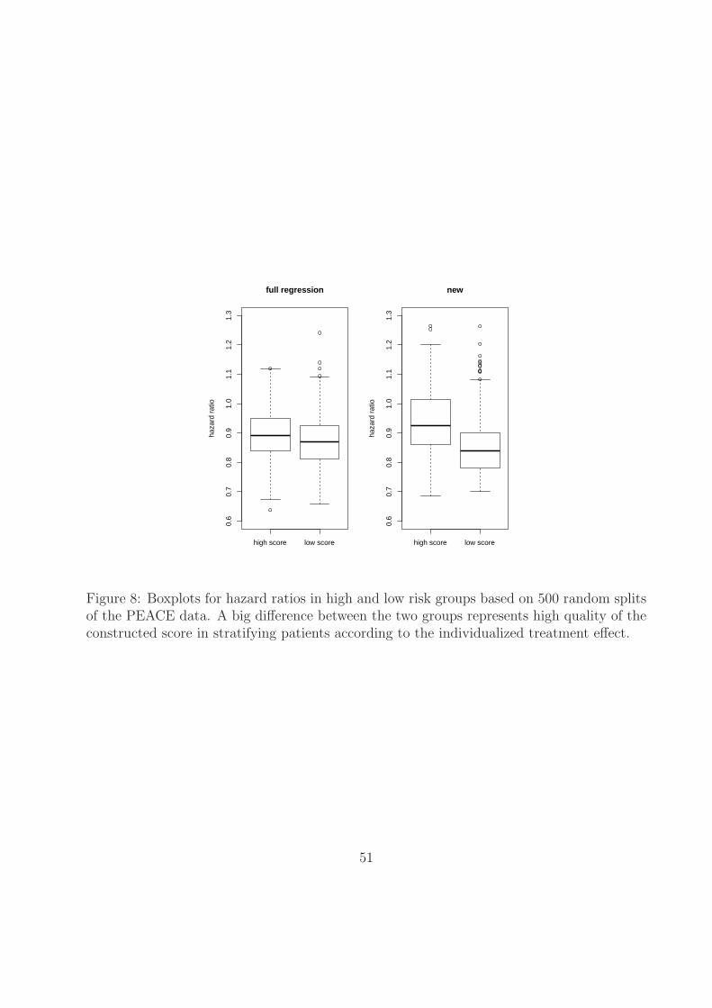
high score low score
0.6
0.7
0.8
0.9
1.0
1.1
1.2
1.3
full regression
haza
rd r
atio
high score low score
0.6
0.7
0.8
0.9
1.0
1.1
1.2
1.3
new
haza
rd r
atio
Figure 8: Boxplots for hazard ratios in high and low risk groups based on 500 random splitsof the PEACE data. A big difference between the two groups represents high quality of theconstructed score in stratifying patients according to the individualized treatment effect.
51
0 1000 2000 3000 4000 5000 6000
0.0
0.2
0.4
0.6
0.8
1.0
low score
time(day)
surv
ival
pro
babi
lity
TamoxifenAlternative
Figure 9: Survival functions of the Tamoxifen and alternative treatment groups: red line,the Tamoxifen group; black line, the alternative treatment arm; thin line, the point-wise95% confidence limits.
52
0 1000 3000 5000
0.0
0.2
0.4
0.6
0.8
1.0
low score
time(day)
surv
ival
pro
babi
lity
0 1000 3000 5000
0.0
0.2
0.4
0.6
0.8
1.0
high score
time(day)su
rviv
al p
roba
bilit
y
0 1000 3000 5000
0.0
0.2
0.4
0.6
0.8
1.0
low score
time(day)
surv
ival
pro
babi
lity
0 1000 3000 5000
0.0
0.2
0.4
0.6
0.8
1.0
high score
time(day)
surv
ival
pro
babi
lity
Figure 10: Survival functions of the Tamoxifen and alternative treatment groups stratifiedby the estimated score in the validation set: red line, the Tamoxifen treatment group; blackline, the alternative treatment group; thin line, the point-wise 95% confidence limits. Upperpanels: the score is based on the “new” method; lower panel: the score is based on “fullregression” method.
53
Recommended