Western University Western University
Scholarship@Western Scholarship@Western
Electronic Thesis and Dissertation Repository
4-19-2013 12:00 AM
A New Diagnostic Test for Regression A New Diagnostic Test for Regression
Yun Shi The University of Western Ontario
Supervisor
Dr. Ian McLeod
The University of Western Ontario
Graduate Program in Statistics and Actuarial Sciences
A thesis submitted in partial fulfillment of the requirements for the degree in Master of Science
© Yun Shi 2013
Follow this and additional works at: https://ir.lib.uwo.ca/etd
Part of the Applied Statistics Commons, Biostatistics Commons, Statistical Methodology Commons,
Statistical Models Commons, and the Statistical Theory Commons
Recommended Citation Recommended Citation Shi, Yun, "A New Diagnostic Test for Regression" (2013). Electronic Thesis and Dissertation Repository. 1238. https://ir.lib.uwo.ca/etd/1238
This Dissertation/Thesis is brought to you for free and open access by Scholarship@Western. It has been accepted for inclusion in Electronic Thesis and Dissertation Repository by an authorized administrator of Scholarship@Western. For more information, please contact [email protected].

A New Diagnostic Test for Regression
(Thesis format: Monograph)
by
Yun Shi
Graduate Program
in
Statistics and Actuarial Science
A thesis submitted in partial fulfillment
of the requirements for the degree of
Master of Science
The School of Graduate and Postdoctoral Studies
The University of Western Ontario
London, Ontario, Canada
© Yun Shi 2013

ABSTRACT
A new diagnostic test for regression and generalized linear models is discussed. The
test is based on testing if the residuals are close together in the linear space of one
of the covariates are correlated. This is a generalization of the famous problem of
spurious correlation in time series regression. A full model building approach for the
case of regression was developed in Mahdi (2011, Ph.D. Thesis, Western University,
”Diagnostic Checking, Time Series and Regression”) using an iterative generalized
least squares algorithm. Simulation experiments were reported that demonstrate the
validity and utility of this approach but no actual applications were developed. In this
thesis, the application of this hidden correlation paradigm is further developed as a
diagnostic check for both regression and more generally for generalized linear models.
The utility of the new diagnostic check is demonstrated in actual applications. Some
simulation experiments illustrating the performance of the diagnostic check are also
presented. It is shown that in some cases, existing well-known diagnostic checks can
not easily reveal serious model inadequacy that is detected using the new approach.
KEY WORDS: diagnostic test, regression, hidden correlation, generalized linear
models
ii

ACKNOWLEDGEMENTS
I would like to express my deep appreciation for my supervisor, Dr. A. Ian McLeod,
who made my Masters degree possible. Because of his endless support, clear guidance
and encouragement, I was able to finish this thesis. Without his help, I would not
have been able to get to where I am now. I would also like to thank my thesis
examiners, Dr. David Bellhouse, Dr. Duncan Murdoch and Dr. John Koval for
carefully reading my thesis and helpful comments. I am also grateful to all faculty,
staff and fellow students at the Department of Statistical and Actuarial Sciences for
their encouragement. Finally, I would like to thank my family for their patience and
love that helped me to get this point.
iii

Contents
ABSTRACT ii
ACKNOWLEDGEMENTS iii
LIST OF TABLES vi
LIST OF FIGURES viii
1 Introduction 11.1 Regression Analysis . . . . . . . . . . . . . . . . . . . . . . . . . . . . 31.2 Linear Regression Model . . . . . . . . . . . . . . . . . . . . . . . . . 3
1.2.1 Important Assumptions . . . . . . . . . . . . . . . . . . . . . 41.2.2 Parameter Estimation . . . . . . . . . . . . . . . . . . . . . . 51.2.3 Regression Diagnostics . . . . . . . . . . . . . . . . . . . . . . 7
2 Test for Hidden Correlation 132.1 Introduction . . . . . . . . . . . . . . . . . . . . . . . . . . . . . . . . 132.2 Kendall Rank Test Method . . . . . . . . . . . . . . . . . . . . . . . 132.3 Pearson Correlation Test Method . . . . . . . . . . . . . . . . . . . . 162.4 Poincare Plot . . . . . . . . . . . . . . . . . . . . . . . . . . . . . . . 172.5 R Package hcc . . . . . . . . . . . . . . . . . . . . . . . . . . . . . . . 18
3 Empirical Error Rates and Power 193.1 Introduction . . . . . . . . . . . . . . . . . . . . . . . . . . . . . . . . 193.2 Parametric Model for Illustrating Hidden Correlation Regression . . . 20
3.2.1 Numerical Example . . . . . . . . . . . . . . . . . . . . . . . . 213.2.2 Maximum Likelihood Estimation . . . . . . . . . . . . . . . . 233.2.3 Generalized Least Squares . . . . . . . . . . . . . . . . . . . . 25
3.3 Empirical Power . . . . . . . . . . . . . . . . . . . . . . . . . . . . . . 28
iv

4 Applications 304.1 Introduction . . . . . . . . . . . . . . . . . . . . . . . . . . . . . . . . 304.2 Estimating Tree Volume . . . . . . . . . . . . . . . . . . . . . . . . . 324.3 Model for Air Quality . . . . . . . . . . . . . . . . . . . . . . . . . . 354.4 Variables Associated with Low Birth Weight . . . . . . . . . . . . . . 424.5 Effect of Gamma Radiation on Chromosomal Abnormalities . . . . . 464.6 Dependence of U.S. City Temperatures on Longitude and Latitude . . 494.7 Species Abundance in the Galapagos Islands . . . . . . . . . . . . . . 534.8 Strength of Wood Beams . . . . . . . . . . . . . . . . . . . . . . . . . 624.9 Rubber Abrasion Loss . . . . . . . . . . . . . . . . . . . . . . . . . . 664.10 Windmill Electrical Output and Wind Speed . . . . . . . . . . . . . . 734.11 Tensile Strength of Paper . . . . . . . . . . . . . . . . . . . . . . . . 764.12 Fisher’s Cat Weight/Heart Data Revisited . . . . . . . . . . . . . . . 804.13 Ozone Pollution in Los Angeles . . . . . . . . . . . . . . . . . . . . . 84
5 Conclusion 875.1 Conclusion . . . . . . . . . . . . . . . . . . . . . . . . . . . . . . . . . 87
Curriculum Vitae 93
v

List of Tables
2.1 Functions in the hcc package . . . . . . . . . . . . . . . . . . . . . . 18
3.1 Ordinary least square model for the simulated data before finding op-timum correlation parameter . . . . . . . . . . . . . . . . . . . . . . . 21
3.2 Generalized least square model for the simulated data . . . . . . . . . 263.3 Hidden correlation test P-value for the generalized least square fit . . 263.4 Comparing the Kendall and LR (likelihood-ratio) tests for different
sample sizes n and correlation parameter r. The percentage of rejectsin 1000 simulations is shown. The maximum standard deviation ofthese percentages is about 1.6. . . . . . . . . . . . . . . . . . . . . . . 29
4.1 Hidden correlation test P-value of the fitted OLS model before logtransformation for the trees data . . . . . . . . . . . . . . . . . . . . 34
4.2 Hidden correlation test P-value for the fitted regression model after logtransformation for the trees data . . . . . . . . . . . . . . . . . . . . 35
4.3 Linear regression model coefficient for airquality . . . . . . . . . . . 354.4 Linear regression model coefficient for the airquality data . . . . . 374.5 Hidden correlation test P-values of the fitted regression model after log
transformation of the response for airquality . . . . . . . . . . . . . 384.6 Hidden correlation test P-value of the final fitted polynomial regression
model for the airquality data . . . . . . . . . . . . . . . . . . . . . 404.7 Rate model for the dicentric data . . . . . . . . . . . . . . . . . . . 474.8 Hidden correlation test P-value of the rate Poisson regression model
for the dicentric data . . . . . . . . . . . . . . . . . . . . . . . . . . 484.9 Hidden correlation test P-value of the fitted multiple regression model
for the ustemp data . . . . . . . . . . . . . . . . . . . . . . . . . . . . 514.10 Hidden correlation test P-value of the fitted multiple regression model
after removing the outlier observation for the ustemp data . . . . . . 514.11 Hidden correlation test P-value of the fitted polynomial regression
model for the ustemp data . . . . . . . . . . . . . . . . . . . . . . . . 524.12 Linear regression model for the gala data after square-root transfor-
mation . . . . . . . . . . . . . . . . . . . . . . . . . . . . . . . . . . . 554.13 Hidden correlation test P-value of the multiple regression model for the
gala data with respect to Elevation . . . . . . . . . . . . . . . . . . 554.14 Hidden correlation test P-value of the multiple regression model after
removing the influential observation for the gala data . . . . . . . . 564.15 Poisson model for gala data . . . . . . . . . . . . . . . . . . . . . . . 58
vi
4.16 Hidden correlation test P-value of the Poisson regression model for thegala data . . . . . . . . . . . . . . . . . . . . . . . . . . . . . . . . . 59
4.17 Hidden correlation tests P-values of the Poisson regression model afterremoving non significant predictors for the gala data . . . . . . . . . 59
4.18 Poisson model after log transformation and variable selection for thegala . . . . . . . . . . . . . . . . . . . . . . . . . . . . . . . . . . . . 59
4.19 Hidden correlation test P-value of the fitted Poisson model after logtransformation and variable selection for gala . . . . . . . . . . . . . 60
4.20 Least squares model for the beams data . . . . . . . . . . . . . . . . . 624.21 Hidden correlation test P-value of the multiple regression model for the
beams data . . . . . . . . . . . . . . . . . . . . . . . . . . . . . . . . 624.22 Least squares model adding a square term for the beams data . . . . 634.23 Hidden correlation test P-value of the multiple regression model after
adding a square term for the beams data . . . . . . . . . . . . . . . . 644.24 Hidden correlation test P-value of the least square fitted model for the
rubber data . . . . . . . . . . . . . . . . . . . . . . . . . . . . . . . . 664.25 Hidden correlation test P-value for least square fitted model after re-
moving unusual observations for the rubber data . . . . . . . . . . . 714.26 Hidden correlation test P-value of bisquare fitted model for the rubber
data . . . . . . . . . . . . . . . . . . . . . . . . . . . . . . . . . . . . 714.27 Least square model for the windmill data . . . . . . . . . . . . . . . 734.28 Hidden correlation test P-value of least square fit for the windmill data 734.29 Hidden correlation test P-value of loess fit for the windmill data . . 744.30 Polynomial regression model for the tensile data . . . . . . . . . . . 764.31 Hidden correlation test P-value of the polynomial regression model for
the tensile data . . . . . . . . . . . . . . . . . . . . . . . . . . . . 764.32 Hidden correlation test P-value of the loess model for the tensile data 784.33 Regression model for the cats data . . . . . . . . . . . . . . . . . . . 804.34 Hidden correlation test P-value of least square fit for the cats data . 804.35 Hidden correlation test P-value for least square fit after removing the
outlier for the cats data . . . . . . . . . . . . . . . . . . . . . . . . . 814.36 Hidden correlation test P-value of the bisquare fit for the cats data . 834.37 Regression model for the ozone data . . . . . . . . . . . . . . . . . . 844.38 Hidden correlation test P-value of the least square fit for ozone data . 85
vii

List of Figures
1.1 Regression model usual diagnostic plots . . . . . . . . . . . . . . . . . 91.2 Usual diagnostic plots for a regression with hidden correlation . . . . 111.3 Poincare plot detects hidden correlation . . . . . . . . . . . . . . . . 12
3.1 Residual dependency plot of e vs. x in the simple regression . . . . . 223.2 Poincare plot diagnostic for correlation among the residuals of the least
square fit before finding optimum correlation parameter . . . . . . . . 233.3 Plot of finding the optimum correlation parameter, r . . . . . . . . . 243.4 Poincare plot using residuals e∗ . . . . . . . . . . . . . . . . . . . . . 26
4.1 Variables relation plot for the trees data . . . . . . . . . . . . . . . . 334.2 Model diagnostic plot for the trees data . . . . . . . . . . . . . . . . 344.3 Explore the relationship between response and each predictor for the
airquality dataset . . . . . . . . . . . . . . . . . . . . . . . . . . . 364.4 Untransformed response on the left; log response on the right . . . . . 374.5 Model diagnostic check before log transformation for the airquality
data . . . . . . . . . . . . . . . . . . . . . . . . . . . . . . . . . . . . 394.6 Model diagnostic check after log transformation for the airquality data 404.7 Chromosomal abnormalities rate response for dicentric . . . . . . . 474.8 Poincare diagnostic plot for correlation among the residuals of the fitted
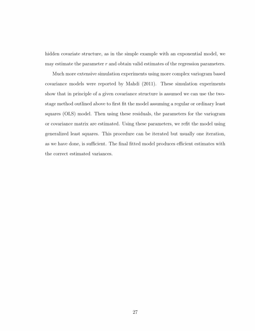
rate Poisson regression model for the dicentric data . . . . . . . . . 484.9 Residuals dependency plot for the dicentric data of the fitted rate
Poisson regression model . . . . . . . . . . . . . . . . . . . . . . . . . 494.10 Model diagnostic plot of the fitted multiple regression model for the
ustemp data . . . . . . . . . . . . . . . . . . . . . . . . . . . . . . . . 504.11 Poincare diagnostic plot for correlation among the residuals of the fitted
multiple regression model for the ustemp data . . . . . . . . . . . . . 514.12 Poincare diagnostic plot for correlation among the residuals of the fitted
polynomial regression model for the ustemp data . . . . . . . . . . . 534.13 Untransformed response on the left and square root transformed re-
sponse on the right . . . . . . . . . . . . . . . . . . . . . . . . . . . . 544.14 Poincare diagnostic plot with respect to Elevation for correlation
among the residuals of the fitted multiple regression model for thegala data . . . . . . . . . . . . . . . . . . . . . . . . . . . . . . . . . 56
4.15 Poincare diagnostic plot with respect to Elevation for correlationamong the residuals of the fitted multiple regression model after re-moving the influential observation for the gala data . . . . . . . . . . 57
viii
4.16 Half-normal plot of the residuals of the Poisson model is shown on theleft ; The relationship between mean and variance is shown on the right 58
4.17 Poincare diagnostic plot for correlation among the residuals of the fittedPoisson regression model after removing non significant predictors forthe gala data . . . . . . . . . . . . . . . . . . . . . . . . . . . . . . . 60
4.18 Poincare diagnostic plot for correlation among the residuals of the fittedpoisson model after log transformation and variable selection for thegala data . . . . . . . . . . . . . . . . . . . . . . . . . . . . . . . . . 61
4.19 Poincare diagnostic plot with respect to x1, gravity, for correlationamong the residuals of the fitted multiple regression model for thebeams data . . . . . . . . . . . . . . . . . . . . . . . . . . . . . . . . 63
4.20 Residuals dependency plot, residuals vs. gravity, for the beams dataof the fitted multiple regression model . . . . . . . . . . . . . . . . . 64
4.21 Poincare diagnostic plot for correlation among the residuals of the fittedmultiple regression model after adding a square term for the beams data 65
4.22 Scatterplot matrix for the rubber data with loess smoother with span =0.7 . . . . . . . . . . . . . . . . . . . . . . . . . . . . . . . . . . . . . 67
4.23 Least square model diagnostic check for the rubber data . . . . . . . 684.24 Poincare diagnostic plot for correlation among residuals of least square
fitted model for the rubber data . . . . . . . . . . . . . . . . . . . . . 684.25 Coplot graphs abrasion loss against tensile strength given hard-
ness for the rubber data . . . . . . . . . . . . . . . . . . . . . . . . . 694.26 Coplot graphs abrasion loss against hardness given tensile strength
for the rubber data . . . . . . . . . . . . . . . . . . . . . . . . . . . . 704.27 Poincare diagnostic plot for correlation among the residuals of bisquare
fitted model for the rubber data . . . . . . . . . . . . . . . . . . . . 724.28 Poincare diagnostic plot for correlation among residuals of least square
fit for the windmill data . . . . . . . . . . . . . . . . . . . . . . . . . 744.29 Poincare diagnostic plot for correlation among residuals of loess fit for
the windmill data . . . . . . . . . . . . . . . . . . . . . . . . . . . . 754.30 Compare the ordinary least square fitted model vs. loess fitted model
for windmill data . . . . . . . . . . . . . . . . . . . . . . . . . . . . . 754.31 Poincare diagnostic plot for correlation among the residuals of the fitted
polynomial regression model for the tensile data . . . . . . . . . . . 774.32 Residual dependency plot of Residuals vs. hardwood . . . . . . . . . 774.33 Poincare diagnostic plot for correlation among the residuals of the loess
fitted model for the tensile data . . . . . . . . . . . . . . . . . . . . 784.34 Compare the ordinary least square fit model vs. loess fit model . . . . 794.35 Poincare diagnostic plot for correlation among the residuals of regres-
sion for the cats data . . . . . . . . . . . . . . . . . . . . . . . . . . 814.36 Residuals dependency plot of Residuals vs. Bwt . . . . . . . . . . . . 824.37 Normal QQ plot on the left, Cooks’s distance plot on the right . . . . 82
ix

4.38 Poincare diagnostic plot with respect to doy for correlation amongresiduals of least square fit for Ozone data . . . . . . . . . . . . . . . 85
x

Introduction
Chapter 1
Introduction
In the construction of statistical models, model validity is critically important to
ensure unbiased and valid statistical inferences. Therefore many model diagnostic
tests have been created for checking and detecting model misspecification. These
tests are extensively discussed in many textbooks on regression such as Atkinson
(1985); Abraham and Ledolter (2006); Cleveland (1993); Faraway (2005, 2006); Sen
and Srivastava (1990); Sheather (2009); Venables and Ripley (2002); Weisberg (1985)
A survey paper of lack-of-fit tests for regression is given by Neill and Johnson (1984).
For example, it sometimes happens that clinical trials yield promising results, but
due to invalid statistical assumptions these promising results prove to be spurious. In
the past, one source of this statistical error in the assumptions was due to the removal
from the study of patients for whom the new test regime did not have positive outcome
(Weir and Murray, 2011) and for this reason medical researchers are required to make
their data available to independent data auditors (Buyse et al., 1999). Interestingly, a
controversy still exists today on whether or not Mendel inadvertently also committed
such an error in his famous genetic experiments with pea plants (Franklin, 2008).
The type of model misspecification discussed in this thesis can also potentially occur
in clinical trials or randomized experiments and result in incorrect inferences. We
should add that we believe this is only a theoretical possibility and does not occur in
practice.
In the absence of statistical independence among observations, the validity of
usual regression models will be threatened. If the assumptions about independence
1

of residuals are violated, the validity of hypothesis testing may not hold. For exam-
ple, ordinary least squares regression assumes errors are independent and normally
distributed with mean of zero and constant variance. If the independence assump-
tions are violated due to undetected correlation among the values of variable, then
unreliable and inefficient estimates of the regression parameters would be obtained.
Furthermore, the statistical tests of these parameters would also be misleading since
ei are correlated so the standard error of the regression coefficients are smaller than
what they should be (Mahdi, 2011, §3.1, 3.4) Consequently, the results will overstate
the precision of the estimates of the parameters.
In this thesis, methods for detecting hidden correlation in regression and, more
generally, in generalized linear models are developed. In the subsequent sections of
this chapter we will discuss and review linear regression analysis, important assump-
tions, and parameter estimation along with regression diagnostics. In Chapter 2,
we will discuss the hidden correlation significance test and a related diagnostic plot
that we call the Poincare plot, named after Henri Poincare. In Chapter 3, we con-
duct a simulation of a simple linear regression model with hidden correlation and we
demonstrate that the least squares estimation method leads to incorrect inferences.
In Chapter 4, we provid a detailed analysis of regression model examples from various
published studies which were examined under the new diagnostic check.
The results in this thesis were obtained using R (R Development Core Team,
2013). Software for the hidden correlation diagnostics as well as the datasets dis-
cussed in this thesis are available in our R package hcc1 (Shi and McLeod, 2013) An
interactive dynamic presentation of the concept of hidden correlation is provided in
our Mathematica demonstration that may be run in a web browser (McLeod and Shi,
1. In this thesis, variable, function and package names in R are indicated by Courierfont, as in hcc.
2

2013).
1.1 Regression Analysis
Regression analysis is used to explain and estimate the relationship among variables.
It can assist in the understanding of how the value of a dependent variable changes
when any one of the independent variable is changed, while other are fixed (Weisberg,
1985). Generally regression analysis is used for making statistical inference and pre-
dicting future observations (Faraway, 2005). Specifically, regression analysis can be
separated into two components: parametric regression and non-parametric regression.
1.2 Linear Regression Model
Linear regression is parametric regression because the regression function is defined
in terms of a finite number of unknown parameters that are estimated from the data.
It was the first type of regression analysis to be studied.
Linear regression attempts to model the relationship between the dependent vari-
able Y and one or more independent or explanatory variables, x1...xp, by fitting a
linear equation to observed data. When p = 1 is called the simple regression and
when p > 1 is called multiple regression. The linear regression model is given as:
y = Xβ + ε (1.1)
where y = (y1, ...yn)′, ε = (ε1, ...εn)
′, β = (β1, ...βp)
′and
X =
1 x1,1 x1,2 · · · x1,p
1 x2,1 x2,2 · · · x2,p...
......
......
1 xn,1 xn,2 · · · xn,p
(1.2)
3

1.2.1 Important Assumptions
Standard linear regression models with standard estimation techniques make a num-
ber of assumptions about the predictor variables, the response variables and their
relationship. When these assumptions are not met the results may not be trustwor-
thy and hypothesis tests based on this model may result in excess Type I or Type
II error rates, or over or under estimation of statistical significance (Abraham and
Ledolter, 2006).
In linear regression model the standard analysis is based on the following assump-
tions about the regressor variable X and the random errors εi, i = 1, . . . , n.
• Absence of Measurement Error: In designed experiments, the predictor
variable is under the experimenters’ control, who can set the value x1, . . . , xn.
xi, i = 1, 2, . . . , n, can be taken as constants, they are fixed values rather than
random variables. So they are assumed not to be contaminated with measure-
ment error. With observational data the predictor variables may or may not
be random but it is assumed that the error in predictor variables is negligible
and there is no correlation between the predictor variable and the random error
term in the model.
• Linearity: The mean of the response variable is a linear combination of the
parameters and the predictor variables. If the relationship between the response
variable and the predictor variables is not linear, the results of the regression
analysis will not be the true relationship.
• Normality: The random errors should follow a normal distribution with mean
0 and variance σ2.
4

• Constant variance: Different response variable have the same variance in
their errors, regardless of the values of the predictor variables. V (εi) = σ2 is
constant for and ui = E(yi) = β0 + β1xi, for all i = 1, 2, . . . , n.
• Independence: This assumes that the errors of the response variable are un-
correlated with each other, which means different errors εi and εj , and hence
different response yi and yj are independent. Cov(εi, εj) = 0 for i 6= j. Viola-
tion of this assumption indicates that the model has specification error and this
misspecification may result in incorrect statistical inference. Lack of indepen-
dence in time series regression may result in spurious regression (Granger and
Newbold, 2001) as in the famous example of the linear regression for predicting
the U.K. stock market index based on car production six months earlier (Box
and Newbold, 1971).
• Multicollinearity: multicollinearity refers to a situation in which two or more
explanatory variables in a multiple regression model are highly linearly related,
which means there have correlated predictor variables in the regression model.
It can also happen if the number of parameters to be estimated more than the
actual data used.
1.2.2 Parameter Estimation
Maximum likelihood estimation is a common method of estimating the parameters
in regression and generalized linear models. In the standard case, it requires inde-
pendent and identically distributed observations. So in linear regression if the errors
are independent and identically normally distributed, then we can use the maximum
likelihood estimation. However, in least square estimation we do not need to refer to
a normal distribution and the Gauss-Markov theorem states that in a linear regres-
5

sion model in which the errors have mean zero and are uncorrelated and have equal
variance, the best linear unbiased estimator of the coefficients is given by the ordinary
least square estimator (Faraway, 2005).
1.2.2.1 Maximum Likelihood Estimation
Maximum likelihood estimation selects the estimates of the parameters to maximize
the likelihood function. We start from simple linear regression; the likelihood function
of the parameters β0, β1, σ2 is the joint probability density function of y1,y2,. . . ,yn,
viewed as a function of the parameters. One looks for values of the parameters that
give us the greatest probability of observing the data (Abraham and Ledolter, 2006).
A probability distribution for y must be specified, we assume that εi has a normal
distribution with mean zero and variance σ2. So we get yi has a normal distribution
with mean u = β0 + β1xi and variance σ2. The probability density function for the
ith response yi is
p(yi|β0, β1, σ2) =
1√2πσ
exp[− 1
2σ2(yi − β0 − β1xi)
2] (1.3)
And the joint probability density function of y1,y2,. . . ,yn is:
p(y1, y2, ..., yn|β0, β1, σ2) = (
1√2π
)σ−2n exp[− 1
2σ2
n∑i=1
(yi − β0 − β1xi)2] (1.4)
Treating this as a function of the parameters leads us to the likelihood function and
its logarithm:
l(β0, β1, σ2) = −n
2log(2π)− n log σ2 − 1
2σ2
n∑i=1
(yi − β0 − β1xi)2 (1.5)
Maximizing the log-likelihood l(β0, β1, σ2) with respect to β0 and β1 is equivalent to
6

minimizing∑ni=1 (yi − β0 − β1xi)
2. The method of estimating β0 and β1 by minimiz-
ing S(β0, β1) =∑ni=1 (yi − β0 − β1xi)
2 is referred to as the method of least squares.
1.2.2.2 Least Squares Estimation
The least squares estimate β of β is chosen to minimize the residual sum of squares.
In general case the least squares estimate of β, called β minimizes:
∑εi
2 = ε′ε = (y −Xβ)
′(y −Xβ) (1.6)
Differentiating with respect to β and setting to zero, we find that β satisfies:
X′Xβ = X
′y (1.7)
Then we get:
β = (X′X)−1X
′y (1.8)
Xβ = X(X′X)−1X
′y (1.9)
y = Hy (1.10)
Where H = X(X′X)−1X
′is called the hat-matrix and is the orthogonal projection
of y onto the space spanned by X. It is an n×n matrix which could be uncomfortably
large for some datasets (Faraway, 2005) and so the fitted values are usually computed
using eqn. (1.9).
1.2.3 Regression Diagnostics
Once we construct a regression model, we may need to confirm that the model fits
the data well. So it may be important to confirm the goodness of fit of the model
and the statistical significance of the estimated parameters.
7

The R-squared statistic provides a useful measure of how well the regression ex-
plains the data and an index of its performance in prediction assuming that statis-
tically all the assumptions discussed earlier are correct (Faraway, 2005). Statistical
significance can be checked by an F-test of the overall fit, followed by t-tests of indi-
vidual parameters. Again these tests rely on our assumptions being valid.
The usually approach to checking our assumptions involves diagnostic checks
(Sheather, 2009) including informal plots such as the normal probability plot to
detect outliers and residual dependency plot to detect model misspecification and
non-constant variance, Cook distances for detecting influential points that result in
misleading conclusions.
In R the plot command produces the model diagnostic plot for us to check the
model adequacy. It is virtually impossible to verify that a given model is exactly
correct but as George Box said “all models are wrong, but some are useful” (Box and
Draper, 1987). The purpose of the diagnostics is more to check whether the model is
not grossly wrong (Faraway, 2006).
1.2.3.1 Dataset trees
We use trees datasets which is a R built-in dataset to illustrate some of the model
diagnostic checks. In Figure 1.1 both left top and bottom plots provide diagnostic
information about whether the variance of the error term appears to be constant.
The only difference between the two plots is whether the residuals are standardized
or not. When points of high leverage exist, instead of looking at residual plots, it is
generally more informative to look at plots of standardized residuals since plots of
the residuals will have nonconstant variance even if the errors have constant variance
(Sheather, 2009). From the residual plot we see that the constant variance assumption
is broken since the residuals getting lager for the trees datasets. The top right plot
8

is the normal QQ plot, the resulting plot produces points close to the straight line
so we may consider the assumption of normality for residuals is satisfied. However,
the normality of the errors assumption is needed in small samples for the validity of
t-distribution based hypothesis test. Witha relatively large sample the central limit
theorem can be invoked such that hypothesis testing may proceed using asymptotic
approximations. The bottom right plot of the standardized residuals against leverage
enables us to readily identify a high leverage point which is also an outlier. From the
plot we may consider the observation 31 is an outlier in the trees data.
10 20 30 40 50 60 70
−5
05
10
Fitted values
Res
idua
ls
Residuals vs Fitted
31
18
2
−2 −1 0 1 2
−1
01
2
Theoretical Quantiles
Sta
ndar
dize
d re
sidu
als
Normal Q−Q
31
18
2
10 20 30 40 50 60 70
0.0
0.5
1.0
1.5
Fitted values
Sta
ndar
dize
d re
sidu
als
Scale−Location31
182
0.00 0.05 0.10 0.15 0.20
−2
−1
01
23
Leverage
Sta
ndar
dize
d re
sidu
als
Cook's distance0.5
0.5
Residuals vs Leverage
31
18
3
Figure 1.1: Regression model usual diagnostic plots
9

1.2.3.2 Simulated hidden correlation dataset
We use our R package hcc to simulate a regression with hidden correlation in a simple
linear regression model, yi = β0 + β1xi + ei, where β0 = β1 = 0, i = 1, . . . , 50, xi
are independent uniform random variables on the interval (0, 50) and ei are normally
distributed with mean zero, variance one and a covariance matrix, Ω = (ω(h(i, j))),
where h(i, j) = |xi − xj |, ω(h) = e−h/r, and r = 5. The following script generates
such a dataset. The regression is highly significant since the p-values correponding
to the prameters are extremely small but this significance is wrong due to the hidden
correlation.
> require("hcc")
> set.seed(313477)
> data <- simer(50, 5)
> ans <- lm(y~x, data=data)
> summary(ans)
Call:
lm(formula = y ~ x, data = data)
Residuals:
Min 1Q Median 3Q Max
-1.15361 -0.32833 0.04064 0.30534 1.44544
Coefficients:
Estimate Std. Error t value Pr(>|t|)
(Intercept) 1.463404 0.185381 7.894 3.18e-10 ***
x -0.035735 0.006066 -5.891 3.67e-07 ***
---
Signif. codes: 0 *** 0.001 ** 0.01 * 0.05 . 0.1 1
Residual standard error: 0.6356 on 48 degrees of freedom
Multiple R-squared: 0.4196, Adjusted R-squared: 0.4075
F-statistic: 34.71 on 1 and 48 DF, p-value: 3.673e-07
The following code fragment produces the usual regression diagnostic plots and
are shown in Figure 1.2. These plots do not strongly signal that there is serious model
10
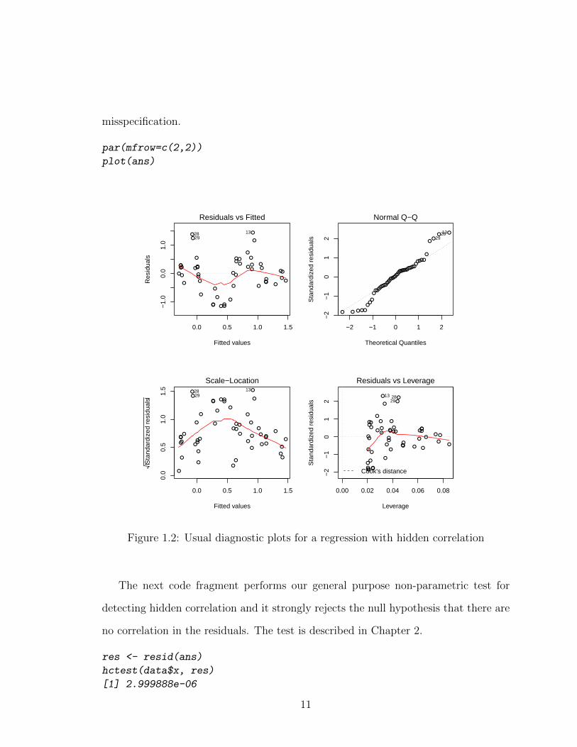
misspecification.
par(mfrow=c(2,2))
plot(ans)
0.0 0.5 1.0 1.5
−1.
00.
01.
0
Fitted values
Res
idua
ls
Residuals vs Fitted
132829
−2 −1 0 1 2−
2−
10
12
Theoretical Quantiles
Sta
ndar
dize
d re
sidu
als
Normal Q−Q
132829
0.0 0.5 1.0 1.5
0.0
0.5
1.0
1.5
Fitted values
Sta
ndar
dize
d re
sidu
als
Scale−Location1328
29
0.00 0.02 0.04 0.06 0.08
−2
−1
01
2
Leverage
Sta
ndar
dize
d re
sidu
als
Cook's distance
Residuals vs Leverage
2829
13
Figure 1.2: Usual diagnostic plots for a regression with hidden correlation
The next code fragment performs our general purpose non-parametric test for
detecting hidden correlation and it strongly rejects the null hypothesis that there are
no correlation in the residuals. The test is described in Chapter 2.
res <- resid(ans)
hctest(data$x, res)
[1] 2.999888e-06
11

The Poincare plot, in Figure 1.3 is a lagged plot of the re-ordered residuals where
the re-ordered residuals have been sorted in ascending order according to the values
of the input x. If the model is adequate, the robust loess line should be approximately
horizontal but instead for the example we see a clear indication of positive dependence
in the residuals indicating severe model inadequacy.
PoincarePlot(data$x, res)
−1.0 −0.5 0.0 0.5 1.0 1.5
−1.
0−
0.5
0.0
0.5
1.0
1.5
e[t]
e[t+
1]
Figure 1.3: Poincare plot detects hidden correlation
12

Test for Hidden Correlation
Chapter 2
Test for Hidden Correlation
2.1 Introduction
In this chapter we will introduce the hidden correlation test method that utilizes the
Kendall rank test and Pearson correlation test. Both tests can be used to detect
hidden correlations in a fitted model. Lastly we will discuss the Poincare plot that
provides a visual diagnostic plot to detect hidden correlation in regression residuals.
These tests and the Poincare plot both use the re-ordered residuals, e(x)j , j =
1, . . . , n, where n is the number of observations. The ordering of these residuals
depends on an input or predictor variable xj , j = 1, . . . , n. Let ej , j = 1, . . . , n
denote the ordinary regression residuals and let πx(j), j = 1, . . . , n be a permutation
of 1, 2, . . . , n that puts x in ascending order. Thus xπx(j) ≥ xπx(j−1), j = 2, . . . , n.
Hence the re-ordered residuals are defined by, e(x)j = eπx(j).
The above procedures are also useful in detecting model inadequacy in general-
ized linear models. In this case, the deviance residuals that is measure of deviance
contributed from each observation are used. Illustrative examples of these diagnostic
checks are provided.
2.2 Kendall Rank Test Method
The Kendall rank (1995) correlation coefficient τ is a rank correlation coefficient that
measures the strength of dependency between two variables and does not require a
linear relationship between those variables. In other words, it is a non-parametric
indication of the degree of monotonic association (Abdi, 2007).
13

Let (x1, y1), (x2, y2), ..., (xn, yn) be a set of observations from the random variable
X and Y . The total number of pairings combinations is n(n−1)/2, Consider ordering
the pairs by x values and then by y values. If any pairs of observations (xi, yj) and
(xj , yj) satisfied that xi > xj and yi > yj or xi < xj and yi < yj then these pairs
are said to be concordant. If xi > xj and yi < yj or xi < xj and yi > yj these pairs
are discordant. If xi = xj and yi = yj the pairs is neither concordant nor discordant.
The Kendall τ coefficient is defined as
τ =nc − nd
n(n− 1)/2(2.1)
where nc is the number of concordant pairs and nd is the number of discordant pairs.
Since the coefficient must be in the range −1 ≤ τ ≤ 1, if τ = 1 then it means the
agreement between the two rankings is perfect. On the other hand, if τ = −1 then
the disagreement between the two rankings is perfect. If X and Y are independent
then we would expect the coefficient to be approximately zero.
If there are identical observations with the same values (tied) then τ is used:
τ =nc − nd√
[n(n− 1)/2−∑ti=1 ti(ti − 1)/2][n(n− 1)/2−
∑ui=1 ui(ui − 1)/2]
(2.2)
where ti is the number of observation tied at a particular rank of x and ui is the
number tied at a rank of y.
The Kendall correlation coefficient is generally used as a test statistic for a hy-
pothesis that determines whether two variables are statistically independent or more
precisely are not associated. It is a non-parametric test since the underlying distribu-
tion for X and Y is not assumed (Siegel, 1957). The test depends only on the order
of the pairs and it can always be computed assuming that one of the rank orders
serves as a reference (Abdi, 2007). The null hypothesis of independence of X and
14

Y states that the sampling distribution of τ converges towards a normal distribution
with mean zero and variance σ2τ when the sample size n is larger than 10. Specifically,
σ2τ can be defined as:
σ2τ =
2(2n+ 5)
9n(n− 1)(2.3)
Transforming τ into a Z score for the null hypothesis test of no tied values we obtain:
Zτ =τ
στ=
τ√2(2n+5)9n(n−1)
(2.4)
This Z value is approximately normally distributed with a mean of 0 and a standard
deviation of 1.
Another type of nonparametric correlation is defined by the Spearman’s ρ (Siegel,
1957) but Kendall’s τ is preferred since convergence to the normal distribution is
much faster. Both R and Mathematica have built-in functions for testing for lack of
association using Kendall’s τ . This test is used in our R package (Shi and McLeod,
2013) as well as our Mathematica demonstration (McLeod and Shi, 2013).
The following code snippet shows how this test is implemented in our R package
hcc Shi and McLeod (2013).
> hctest
function (x, res)
n <- length(x)
stopifnot(n == length(res) && n > 2)
indjx <- order(x)
resx <- res[indjx]
cor.test(resx[-1], resx[-n], method = "kendall")$p.value
15

2.3 Pearson Correlation Test Method
The Pearson product-moment correlation coefficient measures the strength of a linear
association between two variables (Rodgers and Nicewander, 1988). As with Kendall’s
τ , it reflects the direction and strength of the relation between two variables. The
correlation coefficient ranges from -1 to +1. A value of 0 indicates that there is
no association between the two variables. Coefficient values greater than 0 indicate
there is a positive association and values less than 0 indicates a negative association.
The strength of the association of the two variables is reflected by the magnitude
of the coefficient. For example, a coefficient closer to 1 or -1 reflects a stronger
linear association of the two variables. If the two variables are independent, then
the coefficient is 0. However the converse is not true since the correlation coefficient
can only detect linear relationships. While Kendall’s tau is more robust and a more
general test for association, it also can fail to detect lack of independence. For example
both tests fail to detect a V or U shaped dependence in a scatterplot (Franklin, 2008).
The population Pearson correlation coefficient can be expressed as the following:
ρX ,Y =cov(X, Y )
σXσY=E[(X − uX)(Y − uY )]
σXσY(2.5)
When it is applied to a sample, it is represented by r and the formula for the sample
correlation coefficient can be expressed as:
r =
∑ni=1(xi − x)(yi − y)√∑n
i=1(xi − x)2√∑n
i=1(yi − y)2(2.6)
The sampling distribution of Pearson r is approximately normally distributed if the
true correlation between variables X and Y within the general population correlation
equals zero. The sampling distribution of Pearsons correlation coefficient follows a
student t-distribution with a degree of freedom of n − 2. This assumption hold for
16

the null case (zero correlation) even approximately hold if the observed values are
non-normal with not very small sample size.
t = r
√n− 2
1− r2(2.7)
The transformation of the above test equation can then be used to determine the
critical values for r:
r =t√
n− 2 + t2(2.8)
In our R package hcc (Shi and McLeod (2013)) we employ the Kendall rank test
method. Based on a detailed analysis of linear regression examples in Chapter 4, we
prefer to use Kendall rank test method since it is more robust and both methods gave
about the same result.
2.4 Poincare Plot
In linear time series analysis for observed series zt, t = 1, . . . , n, zt may be plotted
against zt−k for t = 2, . . . , n and some fixed k, often k = 1 is of special interest. Such
plot is often used for examining autocorrelation at lag k and it is implemented in base
R in the function lag.plot().
More generally such a plot is known as the Poincare plot and is often used in
nonlinear time series analysis (Tong, 1990). It is a useful graphical tool for detecting
non-linear forms of independence and is widely used in applications (Brennan et al.,
2001).
The Poincare diagnostic plot for checking for hidden correlation is as the scatter-
plot of exj+1 vs. exj . A loess smooth is drawn on the plot to help judge the slope.
Under the assumption of no hidden correlation the plot slope of this line should be
17

approximately zero. Figure 1.3 shows an example when strong hidden correlation is
present. Further examples of this plot are discussed with actual data in Chapter 4.
The code snippet below shows the implementation of this plot in our package hcc
(Shi and McLeod, 2013).
> PoincarePlot
function (x, res)
ind <- order(x)
e <- res[ind]
et <- e[-length(e)]
etp1 <- e[-1]
plot(et, etp1, xlab = "e[t]", ylab = "e[t+1]")
lines(lowess(et, etp1, f = 1), lwd = 2)
invisible()
2.5 R Package hcc
The following functions are available in our package.
Function name Descriptionhctest significance test for hidden correlationPoincarePlot diagnostic plot for hidden correlationrdplot residual dependency plotsimer simulate simple hidden correlation regression
Table 2.1: Functions in the hcc package
18
Empirical Error Rates and Power
Chapter 3
Empirical Error Rates and Power
3.1 Introduction
In this chapter we will show using simulation that in simple linear regression when the
error terms exhibit hidden positive correlation according to the ascending order of one
of the covariates X, then the statistical inferences on the parameter estimates may be
seriously incorrect. It is further shown that our hidden correlation test can detect this
model misspecification or lack of fit. A Mathematica Demonstration (McLeod and Shi,
2013) has also been provided that implements the parametric hidden correlation model
discussed in §3.2. This Demonstration illustrates how spurious statistical inferences
may arise in simple linear regression and that model misspecification due to hidden
correlation may be detected by the Kendall rank test.
In addition to this, we verify the Type I error rate of our test and we investigate
and compare the power of our non-parametric test using the Kendall rank correlation
to a maximum likelihood ratio test when the true model has a specified correlation
structure. Our simulation uses 1000 replications for each test method, sample size,
nominal significant level and correlation parameter. We demonstrate that the sta-
tistical power increases as the sample size increases, as might be expected and also
that the parametric likelihood-ratio test has greater power than the non-parametric
Kendall rank correlation test or the Pearson correlation test.
19

3.2 Parametric Model for Illustrating Hidden CorrelationRegression
A simple example of hidden correlation that may be hard to detect using currently
available regression diagnostics is given the simple exponential correlation model.
This model generalizes the discrete-time first order autoregression, zt = φzt−1 + at,
where at ∼ NID(0, σ2a) to the case of hidden correlation in regression. In this chapter
we will simulate a simple linear regression model with hidden correlation.
Let the response variable be denoted by Y which is a n× 1 vector, where yi can
be modeled as a linear combination of a covariates variable X.
yi = β0 + β1xi + ei, (3.1)
Initially we consider an independent variable, xj , j = 1, . . . , n, that is assumed
to be independent and uniformly distributed on the interval (0, n). Let hj1,j2 =
|xj1−xj2| and define the correlation function ρ(h) = exp−h/r, where h corresponds
to distance and r > 0 is the correlation parameter. It shows that if we take xj , j =
1, . . . , n, then ρ(h) = φh where φ = exp−1/r. This is a special case of the AR(1) in
which the correlation is always positive. More generally, when r = 0, ρ(h) = 0, h > 0
and ρ(0) = 1.
Assume that the errors, e1, . . . , en are multivariate normal with mean vector 0
and covariance matrix Ω. We can define the covariance matrix as
Ω =
σ2Λr r > 0
σ2In r = 0,(3.2)
where Λr = exp−H/r, hj1,j2 = |xj1 − xj2|, and H = (hj1,j2)n×n. When r = 0 the
error variance is equal to σ2In which means there are no hidden correlations among
the residuals.
20

In our simulation, we consider a simple process, we call this the pure hidden
correlation process, where we take β0 = β1 = 0, so we get ei = yi. More generally we
may consider a multiple linear regression in which one of the variables corresponds to
xj and the others are functionally independent of xj .
3.2.1 Numerical Example
In this example, we simulate data with a sample of size n=100, the covariate variable
X is from a uniform distribution. The error terms ei exhibit hidden positive correla-
tions according to the ordered value of the variable X. Initially we set r = 5, σ2 = 1.
First we fit the classical ordinary least square model and we find the parameters are
highly statistical significant as showing in Table 3.1.
Estimate Std. Error t value Pr(>|t|)(Intercept) 0.7557 0.1478 5.1146 0.0000
x -0.0108 0.0025 -4.2687 0.0000
Table 3.1: Ordinary least square model for the simulated data before finding optimumcorrelation parameter
Cleveland (1979) introduced the residual dependency plot by plotting the residuals
versus a covariate variable along with a loess smooth to help visualize whether there
is a relationship. From our simulation the residual dependency plot of Figure 3.1
does not clearly indicate lack-of-fit in that the loess smoother follows a horizontal line
approximately. Looking carefully at Figure 3.1, we do see a nonrandom partern in
the residuals but this could be easy to miss if the correlation parameter r is smaller.
Next we use the hidden correlation test package to conduct a hidden correlation
test by using Kendall rank test method and Pearson correlation test method and
we find the P-value is less than 10−8 for both the Kendall and Pearson tests. The
Poincare plot in Figure 3.2 of the ordered residuals according to the ascending order
21

x
e
−2
−1
0
1
2
0 20 40 60 80 100
Figure 3.1: Residual dependency plot of e vs. x in the simple regression
of the variable x shows very clearly the strong dependence in the residual and is better
at detecting lack-of-fit than the residual dependency plot Figure 3.1.
22

−2 −1 0 1 2
−2
−1
01
2
e[t]
e[t+
1]
Figure 3.2: Poincare plot diagnostic for correlation among the residuals of the leastsquare fit before finding optimum correlation parameter
3.2.2 Maximum Likelihood Estimation
We want to find out the optimum correlation parameter r for the simple exponential
correlation model. In our simulation the exponential correlation model is used to
create the hidden correlation in the error terms of the regression model. The variable
Y is multivariate normal distribution with mean Xβ and covariance matrix Ω. The
probability density function for y is
f(yi) =1
2πn/2|Ω|1/2exp[−1
2(y −Xβ)TΩ−1(y −Xβ)], (3.3)
where r 6= 0, Ω = σ2Λr.
We use the maximum likelihood estimation to get the optimum parameter r for
the covariance matrix. The exact log-likelihood function for r after dropping the
constant terms can be written,
23

L(r, σ2|y) = −n2
log(σ2)− 1
2log det(Λr)−
y′Λr−1y
2σ2. (3.4)
Setting ∂L∂σ2
= 0 and solving, we obtain for the MLE,
σ2 = S/n, (3.5)
where S = y′Λ−1r y, So the exact maximized log-likelihood function for r is given by:
L(r|y) = −n2
log(S/n)− 1
2log det(Λr) (3.6)
Using the data simulated in §3.2.1 we numerically maximized the likelihood to
obtain r = 4.298. The log-likelihood function is shown in Figure 3.3.
0 2 4 6 8 10
88.0
88.5
89.0
89.5
90.0
r
Loglikelihood
Figure 3.3: Plot of finding the optimum correlation parameter, r
We can also conduct a likelihood ratio test. We assume that under the null
hypothesis, there is no hidden correlation then the change in -2(log likelihood) between
the independent error model and the model with hidden correlation should follow a
chi-square distribution with 1 degree of freedom. This test also reports a very small
24

P-value of less than 10−10.
3.2.3 Generalized Least Squares
Next we try to fit the generalized least square model to our simulated data using the
estimated covariance matrix with r = 4.298. We now derive the generalized least
squares estimates from first principles.
Given y = Xβ + e, where we assume y and e are vectors of length n, X is the
n× p design matrix, and β is the p vector of parameters.
This is the general case but we only need to consider the simple regression case.
We assume that the covariance matrix of e is given by Cov (e) = Ω. Let Ω = LL′,
where L is the lower triangular Cholesky decomposition and L′
is its transpose. So
Ω−1 = (L′)−1L−1. Multiplying the model equation we obtain the generalized least
square model:
y∗ = X∗β + e∗ (3.7)
where y∗ = L−1y, X∗ = L−1X, e∗ = L−1e. Hence,
Cov (e∗) = E(e∗(e∗)′) = E(L−1ee
′(L
′)−1) = L−1Ω(L
′)−1 = L−1LL
′(L
′)−1 = In
(3.8)
So eqn. 3.7 can be solved to obtain the least squares estimate for β. This is the
same as the generalized least squares estimate for β in our model eqn. (3.1) assuming
that the parameter r = 4.298 is known in eqn. (3.2). The resulting parameter
estimates and their standard errors are shown in Table 3.2. As expected the estimated
parameters are not significantly different from zero.
We find the P-value corresponding to the parameters are large enough to show
that the covariate variable X is not statistically significant to the fitted GLS model as
25

Estimate Std. Error t value Pr(>|t|)X.s1 -0.1844 0.4763 -0.39 0.6994X.s2 0.0021 0.0082 0.25 0.8029
Table 3.2: Generalized least square model for the simulated data
showing in Table 3.2. The hidden correlation test in Table 3.3 applied to the residuals
e∗ does not indicate model misspecification.
Kendall PearsonX.s1 0.4161 0.4102X.s2 0.8918 0.9050
Table 3.3: Hidden correlation test P-value for the generalized least square fit
The Poincare plot for e∗, Figure 3.4, confirms that there is no misspecification.
−2 −1 0 1 2
−2
−1
01
2
e[t]
e[t+
1]
Figure 3.4: Poincare plot using residuals e∗
This example suggests that a simple linear regression model with hidden corre-
lation can be detected using our hcc package. Moreover, if we assume a parametric
26
hidden covariate structure, as in the simple example with an exponential model, we
may estimate the parameter r and obtain valid estimates of the regression parameters.
Much more extensive simulation experiments using more complex variogram based
covariance models were reported by Mahdi (2011). These simulation experiments
show that in principle of a given covariance structure is assumed we can use the two-
stage method outlined above to first fit the model assuming a regular or ordinary least
squares (OLS) model. Then using these residuals, the parameters for the variogram
or covariance matrix are estimated. Using these parameters, we refit the model using
generalized least squares. This procedure can be iterated but usually one iteration,
as we have done, is sufficient. The final fitted model produces efficient estimates with
the correct estimated variances.
27

3.3 Empirical Power
We compare the Kendall rank test and likelihood ratio test for hidden correlation.
First we simulated the data with hidden correlation and then input to the hcc package
specifying the Kendall rank test method. Also we took the simulated data to the
likelihood ratio test function. In both tests the null hypothesis is that there is no
hidden correlation among the residuals.
We did 1000 simulation replications to find the number of times the null hypothesis
was rejected at the 5% and 1% significant levels. Then we computed the proportion of
rejects of the null hypothesis in both tests as the correlation parameter r is increased
from 0 to 3. The maximum standard deviation for the percentage shown in Table 3.4
is 100×√
0.25/1000.= 1.6
When r = 0, the empirical Type I error rate is estimated. From Table 3.4 we
see that this is not significantly different from the indicated nominal rates of 5% and
1%. For a fixed level and sample size, as r increases the power increases as expected.
Naturally the power is larger for a 5 % test than a 1% test. Also as expected as the
sample size n increases the power increases. Finally, According to Table 3.4 we find
that the likelihood-ratio test outperforms the Kendall rank test.
If indeed it was reasonable to assume that the hidden correlation was generated
by some parametric model such as in eqns. 3.1 and 3.2, then the likelihood-ratio
test would be used. But the major discovery made in this thesis is that the hidden
correlation arising in practice is often due to lack-of-fit and an adequate model may
often be found using a polynomial or regression splines or more generally using a
suitable nonlinear family of models such as generalized additive models, loess or multi-
adaptive regression splines (MARS).
28

r0 0.2 0.5 1 2 3
n = 25nominal 5% test
Kendall 5.3 5.7 14.5 35.3 65.5 75.5LR 3.7 45.2 82.7 96.3 99.6 100
nominal 1% testKendall 0.9 0.9 4.6 15.1 40.2 52.1
LR 1 24.7 62.2 86 98.2 99.5n = 30
nominal 5% testKendall 5.5 6.9 21.3 47.8 78.5 87.5
likelihood-ratio 3.8 55.9 88.4 98.3 99.8 100nominal 1% test
Kendall 0.8 2.1 6.9 26 60.1 72.7LR 0.4 31 71.7 93.9 99.4 99.9
n = 35nominal 5% test
Kendall 4.5 7.8 28.8 61.8 87.7 94likelihood-ratio 3.6 63.3 92.8 99.3 100 100
nominal 1% testKendall 1.1 1.5 11.8 36.9 70.4 83.9
LR 0.6 39.2 79.9 96.7 100 100
Table 3.4: Comparing the Kendall and LR (likelihood-ratio) tests for different samplesizes n and correlation parameter r. The percentage of rejects in 1000 simulations isshown. The maximum standard deviation of these percentages is about 1.6.
29

Applications
Chapter 4
Applications
4.1 Introduction
Detailed analyses of linear regression examples taken from various published sources
are examined with the new diagnostic check. Each section title uses the name of the
dataset that is available in our R package hcc (Shi and McLeod, 2013).
In time series, tests based on the square of the residuals may be used to detect
non-linearity (McLeod and Li, 1983) and such a test is frequently used to test for the
presence of volatility in financial time series (Tsay, 2010, §3.3.1). So we experimented
also with a test based on the square of the residuals but concluded it was not very
helpful since it did not outperform the test using the regular residual.
We also experimented by using the Pearson test as well as the Kendall test. Gen-
erally both tests gave about the same result. We favor using the Kendall test because
it is more robust and more conservative than the Pearson test. Of course if we are
confident that the normality assumption holds, the Pearson test is more appropriate
and has greater statistical power.
In most cases the multiple linear regression model may be written,
yi,j = β0 + β1xi,1 + . . .+ βpxi,p + ei, (4.1)
where i = 1, . . . , n and ei is the error term that is assumed to be normally distributed
with mean zero and constant variance σ2e . Special important cases of this model
include polynomial, and harmonic regression.
30

An extension to logistic regression is discussed in the example in §4.4. Extensions
to many other non-linear models including generalized linear and additive models,
loess models, multi-adaptive regression splines (MARS), and other models discussed
in the celebrated textbook on statistical models in data mining by Hastie et al. (2009).
31

4.2 Estimating Tree Volume
This dataset trees is included in the built-in datasets in R. The data concern the
girth (inches), height, (feet), and volume (cubic feet), of timber in 31 felled black
cherry trees. The corresponding variables are Girth, Height, and Volume respectively.
Girth, is the tree diameter measured at 4ft 6 in above the ground. The objective is
the prediction of Volume from Girth and Height for future trees of the same species.
This dataset was introduced in the book by Ryan et al. (1976) and it was suggested
that a data transformation was needed.
In Figure 4.1 shows the Volume and its logarithm plotted against the other vari-
able. The upper panels indicate a close linear relationship between Volume and Girth
but a less strong linear relationship between Volume and Height. The lower panels
indicate log transformation seems to have stabilized the variance as well as linearized
the relationship.
The standard regression model is shown in the code fragment below along with
the diagnostic plot.
data(trees)
ans<-lm(Volume~Girth+Height, data=trees)
summary(ans)
plot(ans, which=1)
Call:
lm(formula = Volume ~ Girth + Height, data = trees)
Residuals:
Min 1Q Median 3Q Max
-6.4065 -2.6493 -0.2876 2.2003 8.4847
Coefficients:
Estimate Std. Error t value Pr(>|t|)
(Intercept) -57.9877 8.6382 -6.713 2.75e-07 ***
Girth 4.7082 0.2643 17.816 < 2e-16 ***
Height 0.3393 0.1302 2.607 0.0145 *
32

8 10 12 14 16 18 20
1030
5070
Girth
Vol
ume
65 70 75 80 85
1030
5070
Height
Vol
ume
8 10 12 14 16 18 20
2.5
3.0
3.5
4.0
Girth
log(
Vol
ume)
65 70 75 80 85
2.5
3.0
3.5
4.0
Height
log(
Vol
ume)
Figure 4.1: Variables relation plot for the trees data
---
Signif. codes: 0 *** 0.001 **0.01 *0.05 . 0.1 1
Residual standard error: 3.882 on 28 degrees of freedom
Multiple R-squared: 0.948, Adjusted R-squared: 0.9442
F-statistic: 255 on 2 and 28 DF, p-value: < 2.2e-16
Atkinson (1985, Ch. 5) analysis indicates suggests this model is not adequate and
this is verified in the diagnostic plot shown in Figure 4.2.
Our hidden correlation test in both Kendall rank test method and Pearson cor-
relation test method confirm that a usual linear model is not adequate as shown in
Table 4.1. The test result of the ordered successive residuals according to the ascend-
ing order of the variable Height is statistically significant at less than 5 % level in
both Kendall rank test and Pearson correlation test.
33

10 20 30 40 50 60 70
−5
05
10
Fitted values
Res
idua
ls
lm(Volume ~ Girth + Height)
Residuals vs Fitted
31
18
2
Figure 4.2: Model diagnostic plot for the trees data
Kendall PearsonGirth 0.2712 0.1377
Height 0.0236 0.0289
Table 4.1: Hidden correlation test P-value of the fitted OLS model before log trans-formation for the trees data
We take log in both side to get a multiplicative form of the regression model (Sen
and Srivastava, 1990, p.182-183),
log(vi) = β0 + β1 log(h) + β2 log(g) + ei, (4.2)
The transformation worked since our hidden correlation test does not reject model
adequacy as shown in Table 4.2.
34

Kendall PearsonGirth 1.0000 0.8419
Height 0.2413 0.1935
Table 4.2: Hidden correlation test P-value for the fitted regression model after logtransformation for the trees data
4.3 Model for Air Quality
This dataset airquality is also a built-in dataset in R. It was originally assembled in
part by the New York State Department of Conservation and the National Weather
Service. The ozone part was from the New York State Department of Conservation
while the meteorological data was from the National Weather Service. The air quality
data describe the daily air quality measurement in New York by daily readings of the
following air quality values from May 1, 1973 to September 30, 1973. We have n = 154
observations on 6 numerical variables briefly described in Table 4.3.
Ozone Mean Ozone in parts per billion from 1300 to 1500 hours at Roosevelt IslaSolar.R Solar radiationWind Average wind speed in miles per hour at LaGuardia AirportTemp Maximum daily temperature in degrees Fahrenheit at La Guardia AirportMonth Month (1-12)Day Day of month (1-31)
Table 4.3: Linear regression model coefficient for airquality
35

Initially we explore the relationship taking Ozone as the output variable and So-
lar.R, Wind, and Temp as the inputs. These exploratory scatterplots are shown in
Figure 4.3.
0 50 100 200 300
050
100
150
ozone vs rad
rad
ozone
60 70 80 90
050
100
150
ozone vs temp
temp
ozone
5 10 15 20
050
100
150
ozone vs wind
wind
ozone
Figure 4.3: Explore the relationship between response and each predictor for theairquality dataset
From Figure 4.3 we could see some curvature between Ozone and Wind as well as
between Ozone and Temp. According to the book (Faraway, 2005, p.61-63) a standard
linear regression model was fitted to the dataset excluding missing values. Since the
residual diagnostics show some non-constant variance and non-linearity, a logarithmic
transformation of the response variable Ozone is made.
36

The residual vs. fitted value plot comparing the original response and the loga-
rithmic transformed response can be seen in Figure 4.4. The right plot is better than
the left plot for fixing the non constant variable problem.
−20 0 20 40 60 80 100
−50
050
100
Fitted values
Res
idua
ls
Residuals vs Fitted
117
6230
1.5 2.0 2.5 3.0 3.5 4.0 4.5
−2
−1
01
Fitted values
Res
idua
ls
Residuals vs Fitted
21
24117
Figure 4.4: Untransformed response on the left; log response on the right
All parameters are highly statistically significant in the log transformed linear
regression model as showing in Table 4.4 and the residual plot after log transformation
does not indicate any violation of the usual assumptions of the linear regression model.
Estimate Std. Error t value Pr(>|t|)(Intercept) -0.262 0.554 -0.474 0.637Solar.R 0.003 0.001 4.518 0.000
Wind -0.062 0.016 -3.918 0.000Temp 0.049 0.006 8.077 0.000
Table 4.4: Linear regression model coefficient for the airquality data
37

Since this regression is a time series regression it is appropriate to test for the
presence of autocorrelation in the residuals. We use the Durbin-Watson test to check
the assumption of uncorrelated errors. The Durbin-Watson test use the statistic,
d =
∑ni=2(εi − εi−1)2∑n
i=1 ε2i
(4.3)
The test is implemented in the lmtest package.
Durbin-Watson test
data: sqrt(Ozone) ~ Solar.R + Wind + Temp
DW = 1.8726, p-value = 0.2234
alternative hypothesis: true autocorrelation is greater than 0
The Durbin-Watson test result indicates no evidence of correlation among the
residuals
Next a hidden correlation test is conducted as followed in Table 4.5. The Kendall
rank test does not show any problem among the residuals. But the Pearson correla-
tion test failed at 5% significant level when we order the residuals according to the
ascending order of the variable Wind. So we may suspect the errors are correlated.
Kendall PearsonSolar.R 0.2504 0.5634
Wind 0.1087 0.0277Temp 0.2084 0.8611
Table 4.5: Hidden correlation test P-values of the fitted regression model after logtransformation of the response for airquality
38

Next we start with a model having quadratic terms for all three factors including all
of the three 2-way interactions and the one 3-way interaction. Then we use backward
elimination to remove the least significant terms at 5 % significance level. When all
remaining terms contribute significantly to the model we proceed with some model
diagnostics.
0 40 80 120
−50
050
Fitted values
Res
idua
ls
Residuals vs Fitted
117
3086
−2 0 1 2
−2
02
4
Theoretical Quantiles
Sta
ndar
dize
d re
sidu
als
Normal Q−Q
117
30
126
Figure 4.5: Model diagnostic check before log transformation for the airquality data
The diagnostic plots looks like that the variance is not constant and increases with
the mean and the errors are not normalized distributed as show in Figure 4.5. So we
may still need a log transform to the response.
39

After the log transform for Ozone the quadratic term for Temp is no longer sta-
tistically significant so we remove it and fit the model again. This time both usual
model diagnostic test pass as provided in Figure 4.6 and our hidden correlation test
pass as shown in Table 4.6.
2.0 3.0 4.0 5.0
−2
−1
01
Fitted values
Res
idua
ls
Residuals vs Fitted
21
24
143
−2 0 1 2
−4
−2
02
Theoretical Quantiles
Sta
ndar
dize
d re
sidu
als
Normal Q−Q
21
2415
Figure 4.6: Model diagnostic check after log transformation for the airquality data
Kendall PearsonSolar.R 0.4369 0.7191
Wind 0.3619 0.0917Temp 0.0831 0.6165
Table 4.6: Hidden correlation test P-value of the final fitted polynomial regressionmodel for the airquality data
40

The final fitted prediction is,
log(Ozone) = 0.723 + 0.046Temp− 0.22wind + 0.004Solar.R + 0.007Wind2 (4.4)
All coefficients are significant at 5%.
Therefore we may conclude after adding a quadratic term to the variable Wind that
the multiple regression model fit better than before since we remove the correlation
among the ordered residuals accoding to the ascending order of the variable Wind.
41

4.4 Variables Associated with Low Birth Weight
Hosmer and Lemeshow (1989) give a dataset on 189 births at a US hospital, with
the main interest being in low birth weight. This dataset is included in the MASS
package and (Venables and Ripley, 2002, p.194-198) fit the birthwt dataset to show
the relationship between low birth weight baby and mother’s health status.
In the model a response variable, low birth weight, is fitted to 8 explanatory
variables and use a logistic regression (low birth weight (0/1)) response. After fitting
a full logistic regression, Venables and Ripley (2002) use the AIC criterion to get the
final fitted model. We verified their computations in the R code fragment below.
> data(birthwt)
> attach(birthwt)
> race <- factor(race, labels=c("white","black","other"))
> ptd <- factor(ptl >0)
> ftv <- factor(ftv)
> levels(ftv)[-(1:2)] <- "2+"
> bwt <- data.frame(low=factor(low), age, lwt, race, smoke=(smoke>0), ptd,
ht=(ht>0), ui=(ui>0), ftv)
> birthwt.glm <- glm(low ~ ., family=binomial, data=bwt )
> birthwt.step <- step(birthwt.glm, ~ .^2 + I(scale(age)^2)
+ I(scale(lwt)^2),trace=F)
> summary(birthwt.step)
Call:
glm(formula = low ~ age + lwt + smoke + ptd + ht + ui + ftv +
age:ftv + smoke:ui, family = binomial, data = bwt)
Deviance Residuals:
Min 1Q Median 3Q Max
-1.8945 -0.7128 -0.4817 0.7841 2.3418
Coefficients:
Estimate Std. Error z value Pr(>|z|)
(Intercept) -0.582374 1.421613 -0.410 0.682057
age 0.075539 0.053967 1.400 0.161599
lwt -0.020373 0.007497 -2.717 0.006580 **
42

smokeTRUE 0.780044 0.420385 1.856 0.063518 .
ptdTRUE 1.560317 0.497001 3.139 0.001693 **
htTRUE 2.065696 0.748743 2.759 0.005800 **
uiTRUE 1.818530 0.667555 2.724 0.006446 **
ftv1 2.921088 2.285774 1.278 0.201270
ftv2+ 9.244907 2.661497 3.474 0.000514 ***
age:ftv1 -0.161824 0.096819 -1.671 0.094642 .
age:ftv2+ -0.411033 0.119144 -3.450 0.000561 ***
smokeTRUE:uiTRUE -1.916675 0.973097 -1.970 0.048877 *
---
Signif. codes: 0 *** 0.001** 0.01 * 0.05 . 0.1 1
(Dispersion parameter for binomial family taken to be 1)
Null deviance: 234.67 on 188 degrees of freedom
Residual deviance: 183.07 on 177 degrees of freedom
AIC: 207.07
Number of Fisher Scoring iterations: 5
We can see that not all of the predictors are statistically significant at the 5%
significance level. The residual deviance approximates the degrees of freedom, so
there is no overdispersion. Next we check for hidden correlation and we find that
there is hidden correlation present with both age and lwt.
> require("hcc")
> reslm <- resid(birthwt.step)
> hctest(age, reslm)
[1] 1.668773e-08
> hctest(lwt, reslm)
[1] 0.001061381
Venables and Ripley (2002, p.194-198) do not provide any residual diagnostic tests
that indicate lack of fit in their original model but they do examine possible lack of
fit by fitting a GAM (generalized additive model) to this data. Although Venables
and Ripley (2002, p.194-198) used S-PLUS, we were able to reproduce their results
using the package gam (Hastie, 2013) in R. The R code and result are given below.
43

#test for hidden correlation
> require("gam")
> age1 <- age*(ftv=="1"); age2 <- age*(ftv=="2+")
> birthwt.gam <- gam(low ~ s(age) + s(lwt) + smoke + ptd + ht
+ ui + ftv + s(age1)+s(age2)+smoke:ui, binomial, bwt, maxit=25)
> summary(birthwt.gam)
Call: gam(formula = low ~ s(age) + s(lwt) + smoke + ptd + ht + ui +
ftv + s(age1) + s(age2) + smoke:ui, family = binomial, data = bwt,
maxit = 25)
Deviance Residuals:
Min 1Q Median 3Q Max
-2.0265 -0.7177 -0.4521 0.7623 2.2081
(Dispersion Parameter for binomial family taken to be 1)
Null Deviance: 234.672 on 188 degrees of freedom
Residual Deviance: 170.0319 on 164.9998 degrees of freedom
AIC: 218.0322
Number of Local Scoring Iterations: 14
DF for Terms and Chi-squares for Nonparametric Effects
Df Npar Df Npar Chisq P(Chi)
(Intercept) 1
s(age) 1 3 3.1154 0.3742
s(lwt) 1 3 2.5100 0.4735
smoke 1
ptd 1
ht 1
ui 1
ftv 2
s(age1) 1 3 3.3766 0.3371
s(age2) 1 3 3.1522 0.3688
smoke:ui 1
Venables and Ripley (2002, Figure 7.2) reproduce the standard residual diagnostic
test that are available in R via the function plot.gam and they conclude: “Both the
summary and the plots show no evidence of non-linearity”. However our hidden-
correlation tests tell another story.
44

> resgam <- resid(birthwt.gam)
> hctest(age, resgam)
[1] 3.885305e-09
> hctest(lwt, resgam)
[1] 0.0006595008
Further work is needed to develop an adequate model for this data. It is hoped
to include this in a forthcoming paper.
45

4.5 Effect of Gamma Radiation on ChromosomalAbnormalities
In Purott and Reeder (1976), some data are presented from an experiment conducted
to determine the effect of gamma radiation on the number of chromosomal abnormal-
ities observed. This data is available in our package (Shi and McLeod, 2013) in the
dataframe dicentric. The variables included are:
ca: number of chromosomal abnormalities
cell: the number cells, in hundreds of cells, exposed in each run
dose: dose amount
doserate: rate at which dose is applied
Initially we can format the data to take a look:
> (round(xtabs(ca/cells ~ doseamt+doserate, dicentric),2))
doserate
doseamt 0.1 0.25 0.5 1 1.5 2 2.5 3 4
1 0.05 0.05 0.07 0.07 0.06 0.07 0.07 0.07 0.07
2.5 0.16 0.28 0.29 0.32 0.38 0.41 0.41 0.37 0.44
5 0.48 0.82 0.90 0.88 1.23 1.32 1.34 1.24 1.43
Since there is a multiplicative effect of the dose rate as Figure 4.7 shows.
A rate model is fitted to the dataset by modelling the rate of chromosomal abnor-
malities while maintaining the count response and fix the coefficient log cells and log
the variable doserate. As can be seen from the model summary from Table 4.7 all of
the predictors are statistically significant and the residual deviance is 21.75 which is
close to its 21 degree of freedom. (Faraway, 2006, p.61-63) claims the model fits well.
Next we conduct a hidden correlation test by ordering the non-factor variable
doserate to get the ordered deviance residuals. As can be seen from the Table 4.8
46

0.0
0.4
0.8
1.2
doseamt
mea
n of
ca/
cells
1 2.5 5
doserate
42.5231.50.510.250.1
Figure 4.7: Chromosomal abnormalities rate response for dicentric
Estimate Std. Error z value Pr(>|z|)(Intercept) -2.7467 0.0343 -80.16 0.0000
log(doserate) 0.0718 0.0352 2.04 0.0413dosef2.5 1.6254 0.0495 32.86 0.0000
dosef5 2.7611 0.0435 63.49 0.0000log(doserate):dosef2.5 0.1612 0.0483 3.34 0.0008
log(doserate):dosef5 0.1935 0.0424 4.56 0.0000
Table 4.7: Rate model for the dicentric data
the test results for both Kendall rank test and Pearson correlation test of the ordered
deviance residuals are statistically significant at 1% level. We conclude that there is
significant correlation among the deviance residuals.
Also the Poincare plot of Figure 4.8 shows the positive correlation among the
ordered deviance residuals with respect to doserate.
However, the residual dependency plot for residuals vs. doserate Figure 4.9 does
not strongly suggest a dependency problem.
47

kendall pearsondoserate 0.0162 0.0098
Table 4.8: Hidden correlation test P-value of the rate Poisson regression model forthe dicentric data
−1.5 −1.0 −0.5 0.0 0.5 1.0 1.5
−1.
5−
0.5
0.5
1.5
e[t]
e[t+
1]
Figure 4.8: Poincare diagnostic plot for correlation among the residuals of the fittedrate Poisson regression model for the dicentric data
Our hidden correlation test result clearly reveals that there is significant positive
dependence in the residuals and so statistical inferences from the fitted model may
not be correct. Therefore we may consider the fitted rate model is not good enough
for the dicentric data.
In a forthcoming article, we investigate if the model can be improved used regres-
sion splines (Hastie et al., 2009) or possibly using the extended family of generalized
additive models discussed in the books Hastie and Tibshirani (1990); Wood (2006)
and implemented in the R packages Hastie (2013); Wood (2012).
48
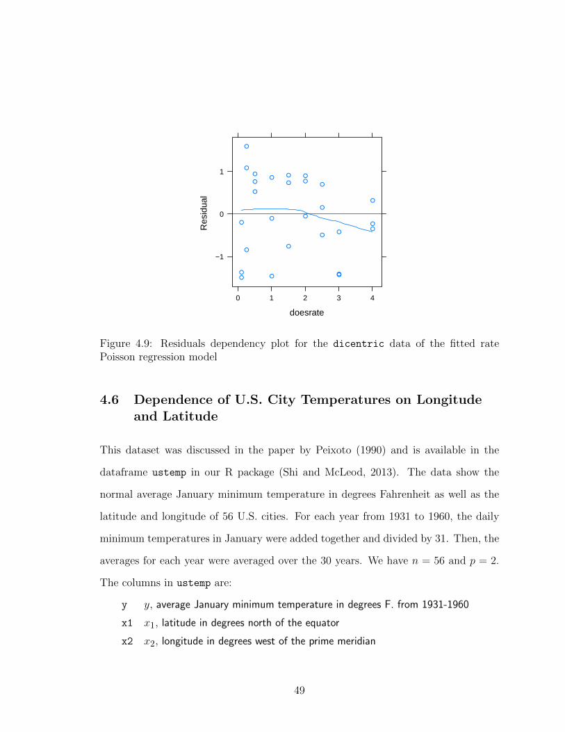
doesrate
Res
idua
l
−1
0
1
0 1 2 3 4
Figure 4.9: Residuals dependency plot for the dicentric data of the fitted ratePoisson regression model
4.6 Dependence of U.S. City Temperatures on Longitudeand Latitude
This dataset was discussed in the paper by Peixoto (1990) and is available in the
dataframe ustemp in our R package (Shi and McLeod, 2013). The data show the
normal average January minimum temperature in degrees Fahrenheit as well as the
latitude and longitude of 56 U.S. cities. For each year from 1931 to 1960, the daily
minimum temperatures in January were added together and divided by 31. Then, the
averages for each year were averaged over the 30 years. We have n = 56 and p = 2.
The columns in ustemp are:
y y, average January minimum temperature in degrees F. from 1931-1960
x1 x1, latitude in degrees north of the equator
x2 x2, longitude in degrees west of the prime meridian
49

A linear regression model using latitude and longitude was fit,
y = 98.645− 2.164x1 + 0.134x2. (4.5)
All the predictors are statistically significant in the fitted regression model and
the model explains well with R2 = 73%. The usual model diagnostic checks, shown
in Figure 4.10, do not provide any strong indication of lack-of-fit.
10 20 30 40 50
0.0
0.5
1.0
1.5
Fitted values
Sta
ndar
dize
d re
sidu
als
Scale−Location52
41
32
−2 −1 0 1 2
−2
−1
01
23
4
Theoretical Quantiles
Sta
ndar
dize
d re
sidu
als
Normal Q−Q
52
41
32
Figure 4.10: Model diagnostic plot of the fitted multiple regression model for theustemp data
But when the residuals are ordered according to the ascending order of the vari-
able longitude both Kendall rank test and Pearson correlation test are statistically
significant at the 5 % level, even the squared Kendall and Pearson tests are also sta-
tistically significant at 1% and 5 % level respectively as can be seen in Table 4.9.
From the hidden correlation test we may suspect the residuals are not independent
in the least square fitted model.
The Poincare plot of Figure 4.11 also verifies the positive correlation in the ordered
50
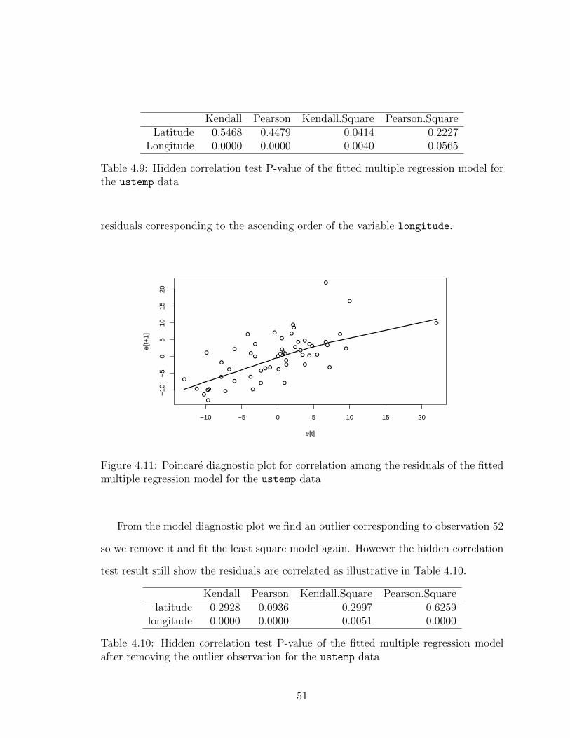
Kendall Pearson Kendall.Square Pearson.SquareLatitude 0.5468 0.4479 0.0414 0.2227
Longitude 0.0000 0.0000 0.0040 0.0565
Table 4.9: Hidden correlation test P-value of the fitted multiple regression model forthe ustemp data
residuals corresponding to the ascending order of the variable longitude.
−10 −5 0 5 10 15 20
−10
−5
05
1015
20
e[t]
e[t+
1]
Figure 4.11: Poincare diagnostic plot for correlation among the residuals of the fittedmultiple regression model for the ustemp data
From the model diagnostic plot we find an outlier corresponding to observation 52
so we remove it and fit the least square model again. However the hidden correlation
test result still show the residuals are correlated as illustrative in Table 4.10.
Kendall Pearson Kendall.Square Pearson.Squarelatitude 0.2928 0.0936 0.2997 0.6259
longitude 0.0000 0.0000 0.0051 0.0000
Table 4.10: Hidden correlation test P-value of the fitted multiple regression modelafter removing the outlier observation for the ustemp data
51

A polynomial regression model was suggested by Peixoto (1990). The author
suggest a model in which a linear relationship is assumed between temperature and
latitude; then, after adjusting for latitude, a cubic polynomial in longitude accurately
predicts the temperature.
y = 262.6−23.85x1−4.286x2+0.73x1x2+0.048x22−0.008x1x
22−0.0002x3
2+0.00003x1x32,
(4.6)
This model passes the hidden correlation test as showing in Table 4.11.
Kendall Pearson Kendall.Square Pearson.SquareLatitude 0.6790 0.8397 0.4723 0.1173
Longitude 0.8219 0.9517 0.3957 0.7470
Table 4.11: Hidden correlation test P-value of the fitted polynomial regression modelfor the ustemp data
The Poincare plot of Figure 4.12 also confirms that there does not have correlation
left among the residuals.
From our hidden correlation test result we may consider the polynomial regression
model is a better fit for the ustemp dataset.
52

−4 −2 0 2 4 6
−4
−2
02
46
e[t]
e[t+
1]
Figure 4.12: Poincare diagnostic plot for correlation among the residuals of the fittedpolynomial regression model for the ustemp data
4.7 Species Abundance in the Galapagos Islands
This dataset, gala (Shi and McLeod, 2013), was presented by Johnson and Raven
(1973) and is discussed in the book (Faraway, 2005, p. 18–20). There are 30 Galapagos
islands and 7 variables in the dataset. The relationship between the number of plant
species and several geographic variables is of interest. The original dataset contained
several missing values which have been filled for convenience in the book Faraway
(2005, p.18-20). We have n = 30 and p = 6 and the following variables:
53

Species number of plant species found on the island
Endemics number of endemic species
Area area of the island, km2
Elevation highest elevation of the island, m
Nearest distance from the nearest island, km
Scruz distance from Santa Cruz island, km
Adjacent area of the adjacent island, km2
We model the number of species using normal linear regression and we see clear
evidence of nonconstant variance shown in the left panel of Figure 4.13. A Box-Cox
analysis (Box and Cox, 1964) reveals that a square root transformation is the best.
This is verified in the right panel of Figure 4.13.
0 100 200 300 400
−10
00
5010
015
020
0
Fitted values
Res
idua
ls
Residuals vs Fitted
SantaCruz
Pinta
SantaMaria
5 10 15 20
−4
−2
02
46
Fitted values
Res
idua
ls
Residuals vs Fitted
SantaCruzGardner1
Pinta
Figure 4.13: Untransformed response on the left and square root transformed responseon the right
In the square transformed model not all of the predictors are statistically signifi-
cant as showing in Table 4.12. But a fairly good fit with R2 = 0.78 is obtained.
We conduct the hidden correlation test in the new fitted model after using square-
54

Estimate Std. Error t value Pr(>|t|)(Intercept) 3.3919 0.8713 3.89 0.0007
Area -0.0020 0.0010 -1.93 0.0651Elevation 0.0165 0.0024 6.75 0.0000
Nearest 0.0249 0.0479 0.52 0.6078Scruz -0.0135 0.0098 -1.38 0.1815
Adjacent -0.0034 0.0008 -4.18 0.0003
Table 4.12: Linear regression model for the gala data after square-root transformation
root transformation. The test shown Table 4.13 reveals that the residuals are corre-
lated with both the Kendall and Pearson tests at 5% significance level when ordering
the residuals according to the ascending order of the variable Elevation.
Kendall PearsonArea 0.2397 0.0955
Elevation 0.0201 0.0375Nearest 0.6156 0.3298
Scruz 0.6156 0.6870Adjacent 0.6420 0.9009
Table 4.13: Hidden correlation test P-value of the multiple regression model for thegala data with respect to Elevation
55

The Poincare plot of Figure 4.14 also confirms the correlation among the ordered
residuals corresponding to the ascending order of the variable Elevation.
−4 −2 0 2 4
−4
−2
02
4
e[t]
e[t+
1]
Figure 4.14: Poincare diagnostic plot with respect to Elevation for correlation amongthe residuals of the fitted multiple regression model for the gala data
An examination of the Cook distances for the least squares fit shows the island
of Isabela to be very influential and we exclude this island from the least squares
fit (Faraway, 2005, p.104). This time our hidden correlation test passes as shown in
Table 4.14.
Kendall PearsonArea 0.8602 0.4340
Elevation 0.3991 0.3993Nearest 0.2980 0.7218
Scruz 0.9532 0.7809Adjacent 0.9221 0.8602
Table 4.14: Hidden correlation test P-value of the multiple regression model afterremoving the influential observation for the gala data
56

The Poincare plot, Figure 4.15, confirms lack of correlation among the residuals
with respect to Elevation.
−4 −2 0 2 4
−4
−2
02
4
e[t]
e[t+
1]
Figure 4.15: Poincare diagnostic plot with respect to Elevation for correlation amongthe residuals of the fitted multiple regression model after removing the influentialobservation for the gala data
Following (Faraway, 2006, p. 57-60), we examine the Poisson regression model for
the Galapagos data. We find all the predictors are highly statistically significant as
showing in Table 4.15. But the residual deviance is 717 on 24 degree of freedoms,
which indicates an ill fitting model. We checked the residuals to see if the large
deviance can be explained and also checked the mean and variance assumption for
the Poisson model.
The half-normal plot of Figure shows no outliers, but the variance assumption of
Poisson regression model is broken since the variance is proportional to but larger
than the mean. In that case overdispersion would occur.
The overdispersion can arise from the violation of independent or identical as-
57

Estimate Std. Error z value Pr(>|z|)(Intercept) 3.1548 0.0517 60.96 0.0000
Area -0.0006 0.0000 -22.07 0.0000Elevation 0.0035 0.0001 40.51 0.0000Nearest 0.0088 0.0018 4.85 0.0000Scruz -0.0057 0.0006 -9.13 0.0000
Adjacent -0.0007 0.0000 -22.61 0.0000
Table 4.15: Poisson model for gala data
0.0 0.5 1.0 1.5 2.0
02
46
810
Half−normal quantiles
Sor
ted
Dat
a
27
11
2.5 3.5 4.5 5.5
02
46
810
µ
(y−
µ)2
Figure 4.16: Half-normal plot of the residuals of the Poisson model is shown on theleft ; The relationship between mean and variance is shown on the right
sumption or dependency between trails (Faraway, 2006). Next we conduct our hid-
den correlation test to see if the residuals are correlated. Our hidden correlation test
shows that the ordered successive residuals are correlated in both Kendall and Pear-
son tests at the 5% significance level according to the order of the variable Elevation
as shown in Table 4.16.
Adjusting the standard errors by the dispersion parameter and using the F-test we
see both the predictors Nearest and Scruz relative to the full model are not statisti-
58

Kendall PearsonArea 0.6156 0.4288
Elevation 0.0301 0.0286Nearest 0.1974 0.2938
Scruz 0.8965 0.8305Adjacent 0.8380 0.6889
Table 4.16: Hidden correlation test P-value of the Poisson regression model for thegala data
cally significant. So we use backward elimination to remove the most non-significant
predictors. Finally we fit the Poisson model with three predictors Area, Elevation
and Adjacent. However, overdispersion still exists and the hidden correlation test in
Table 4.17 still indicates the dependency among the residuals
Kendall PearsonArea 0.6156 0.4870
Elevation 0.0879 0.0330Adjacent 0.5392 0.6095
Table 4.17: Hidden correlation tests P-values of the Poisson regression model afterremoving non significant predictors for the gala data
The Poincare plot of Figure 4.17 also shows the residuals dependency.
The author finds a log transformation of all the predictors is helpful because the
result is a substantial reduction in the deviance from previous 716.85 to 359.54. The
final model, Table 4.18, uses the log transformation and backwards variable selection
by the AIC criteria.
Estimate Std. Error z value Pr(>|z|)(Intercept) 3.2767 0.0441 74.25 0.0000
log(Area) 0.3750 0.0080 46.74 0.0000log(Adjacent) -0.0957 0.0061 -15.65 0.0000
Table 4.18: Poisson model after log transformation and variable selection for the gala
59

−10 −5 0 5 10
−10
−5
05
10
e[t]
e[t+
1]
Figure 4.17: Poincare diagnostic plot for correlation among the residuals of the fittedPoisson regression model after removing non significant predictors for the gala data
Our hidden correlation test result, Table 4.19, shows the P-value for the ordered
residuals according to the ascending order of the variable Area is just less than 0.05,
which indicates there may still remaining slight correlation among the residuals.
Kendall PearsonArea 0.0685 0.0494
Adjacent 0.5896 0.5849
Table 4.19: Hidden correlation test P-value of the fitted Poisson model after logtransformation and variable selection for gala
The Poincare plot, Figure 4.18, confirms that a small degree of correlation still
remains.
From our hidden correlation test we may consider that the least squares fitted
model after removing the influential observation is better than the Poisson regression
model for the gala data. The hidden correlation test is useful in detecting overdis-
60
−5 0 5
−5
05
e[t]
e[t+
1]
Figure 4.18: Poincare diagnostic plot for correlation among the residuals of the fittedpoisson model after log transformation and variable selection for the gala data
persion in Poisson regression models.
61
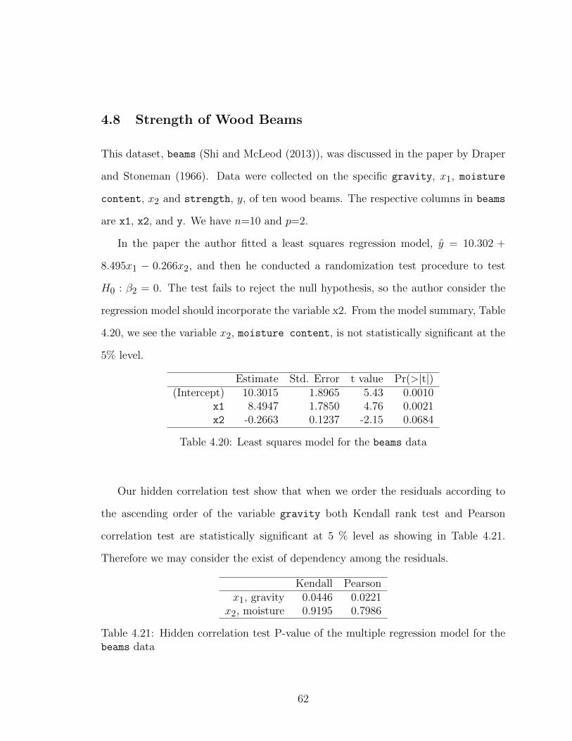
4.8 Strength of Wood Beams
This dataset, beams (Shi and McLeod (2013)), was discussed in the paper by Draper
and Stoneman (1966). Data were collected on the specific gravity, x1, moisture
content, x2 and strength, y, of ten wood beams. The respective columns in beams
are x1, x2, and y. We have n=10 and p=2.
In the paper the author fitted a least squares regression model, y = 10.302 +
8.495x1 − 0.266x2, and then he conducted a randomization test procedure to test
H0 : β2 = 0. The test fails to reject the null hypothesis, so the author consider the
regression model should incorporate the variable x2. From the model summary, Table
4.20, we see the variable x2, moisture content, is not statistically significant at the
5% level.
Estimate Std. Error t value Pr(>|t|)(Intercept) 10.3015 1.8965 5.43 0.0010
x1 8.4947 1.7850 4.76 0.0021x2 -0.2663 0.1237 -2.15 0.0684
Table 4.20: Least squares model for the beams data
Our hidden correlation test show that when we order the residuals according to
the ascending order of the variable gravity both Kendall rank test and Pearson
correlation test are statistically significant at 5 % level as showing in Table 4.21.
Therefore we may consider the exist of dependency among the residuals.
Kendall Pearsonx1, gravity 0.0446 0.0221
x2, moisture 0.9195 0.7986
Table 4.21: Hidden correlation test P-value of the multiple regression model for thebeams data
62

The resulting Poincare plot of Figure 4.19 also indicates the dependency among
the ordered residuals according to the ascending order of the variable gravity.
−0.4 −0.2 0.0 0.2 0.4
−0.
40.
00.
20.
4
e[t]
e[t+
1]
Figure 4.19: Poincare diagnostic plot with respect to x1, gravity, for correlation amongthe residuals of the fitted multiple regression model for the beams data
However, the residuals dependence plot of Figure 4.20 does not show any correla-
tion among the residuals.
Next we try to fit a quadratic model by adding a square term to the variable x2,
moisture content, and we see all the predictors are highly statistical significant and
the R2 = 98% also confirms the model fitted well as shown in Table 4.22.
Estimate Std. Error t value Pr(>|t|)(Intercept) -42.5951 8.4936 -5.01 0.0024
x1 9.6817 0.7285 13.29 0.0000x2 10.4282 1.7112 6.09 0.0009
I(x2^2) -0.5422 0.0867 -6.25 0.0008
Table 4.22: Least squares model adding a square term for the beams data
63

gravity
Res
idua
l for
str
engt
h of
bea
m
−0.4
−0.2
0.0
0.2
0.4
0.40 0.45 0.50 0.55 0.60
Figure 4.20: Residuals dependency plot, residuals vs. gravity, for the beams data ofthe fitted multiple regression model
Our hidden correlation test using both Kendall rank test and Pearson correlation
test does not detect any problem among the residuals as shown in Table 4.23.
Kendall Pearsongravity 0.4767 0.8484
moisture 0.1802 0.2422
Table 4.23: Hidden correlation test P-value of the multiple regression model afteradding a square term for the beams data
The Poincare plot of Figure 4.21 also confirms that there is no correlation among
the residuals.
From our hidden correlation test, we may consider the least squares fitted model
after adding a square term to the variable x2, moisture content, is better than
before adding a square term to the variable x2 for the beams data.
64
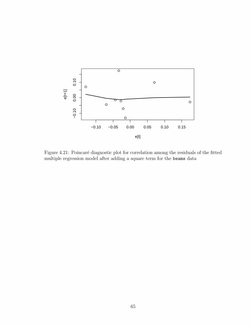
−0.10 −0.05 0.00 0.05 0.10 0.15
−0.
100.
000.
10
e[t]
e[t+
1]
Figure 4.21: Poincare diagnostic plot for correlation among the residuals of the fittedmultiple regression model after adding a square term for the beams data
65

4.9 Rubber Abrasion Loss
This is a famous dataset and was discussed in the book by Cleveland (1993, p.180-187)
and references therein and available as rubber (Shi and McLeod, 2013). The data
come from an experiment to investigate how the resistance of rubber to abrasion is
affected by the hardness of the rubber and its tensile strength. Each of 30 samples of
rubber was tested for hardness and for tensile strength, and then subjected to steady
abrasion for a fixed time. We have n=30 and p=2.
First a scatterplot matrix in Figure 4.22 displays the trivariate data: measure-
ment of abrasion loss, hardness, and tensile strength for 30 rubber specimens that
correspond to the variables abrasion.loss, hardness, and tensile.strength in
the dataframe rubber.
When we fit a linear regression model with the two explanatory variables hard-
ness and tensile strength we find that both predictors are highly statistically
significant. The adjusted R2 = 0.82 suggests the model explains the data quite well.
Considering the usual model diagnostic test as provided in Figure 4.23 we do not
see any obvious violation to the usual model assumptions such as lack of constant
error variance or non-normality. But we notice from the normal QQ plot, right panel
Figure 4.23, that there may be unusual observations.
Our hidden correlation test does not pass at the 5% significant level, as shown in
Table 4.24, since with the Kendall rank test the P-value is 4.8% for tensile.strength
and 6.6% for the Pearson correlation test.
Kendall Pearsonhardness 0.2878 0.2355
tensile.strength 0.0482 0.0666
Table 4.24: Hidden correlation test P-value of the least square fitted model for therubber data
66
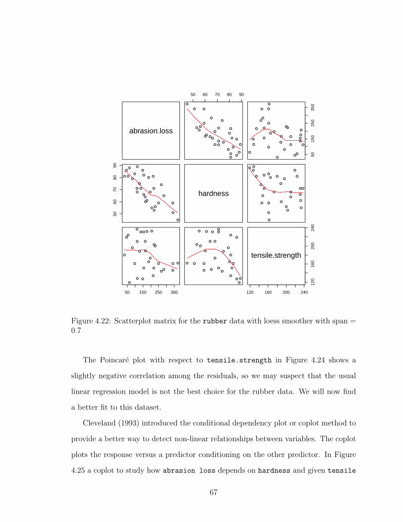
abrasion.loss
50 60 70 80 90
5015
025
035
0
5060
7080
90
hardness
50 150 250 350
120 160 200 240
120
160
200
240
tensile.strength
Figure 4.22: Scatterplot matrix for the rubber data with loess smoother with span =0.7
The Poincare plot with respect to tensile.strength in Figure 4.24 shows a
slightly negative correlation among the residuals, so we may suspect that the usual
linear regression model is not the best choice for the rubber data. We will now find
a better fit to this dataset.
Cleveland (1993) introduced the conditional dependency plot or coplot method to
provide a better way to detect non-linear relationships between variables. The coplot
plots the response versus a predictor conditioning on the other predictor. In Figure
4.25 a coplot to study how abrasion loss depends on hardness and given tensile
67

50 150 250 350
−50
050
Fitted values
Res
idua
ls
Residuals vs Fitted
1914
28
−2 −1 0 1 2
−2
−1
01
2
Theoretical QuantilesS
tand
ardi
zed
resi
dual
s
Normal Q−Q
19
14
28
Figure 4.23: Least square model diagnostic check for the rubber data
−50 0 50
−50
050
e[t]
e[t+
1]
Figure 4.24: Poincare diagnostic plot for correlation among residuals of least squarefitted model for the rubber data
strength is shown. Abrasion loss is graphed against tensile strength for those
observations whose values of hardness lie in a given interval that is determined by
68

equal-count algorithm (Cleveland, 1993, p.134). We use the R lattice package. This
package contains numerous functions that allow for the creation of various conditional
plots beyond just simple scatterplots.
Tensile Strength (kg/square cm)
Abr
asio
n Lo
ss (
g/hp
−ho
ur)
100
200
300
120 140 160 180 200 220 240
Hardness
Hardness
120 140 160 180 200 220 240
Hardness
Hardness
120 140 160 180 200 220 240
Hardness
100
200
300
Hardness
Hardness (degrees Shore)
Pan
el
1
2
3
4
5
6
50 60 70 80 90
Figure 4.25: Coplot graphs abrasion loss against tensile strength given hard-
ness for the rubber data
In the coplot in Figure 4.25, except for the upper right panel, the dependence
of abrasion loss on tensile strength given hardness indicates a linear pattern
below and above 180 kg/cm2 and the pattern shifts up and down but does not change
the overall trend. However, the upper right panel shows a departure from the pattern
since the lowest three values of tensile strength pull down the line.
69
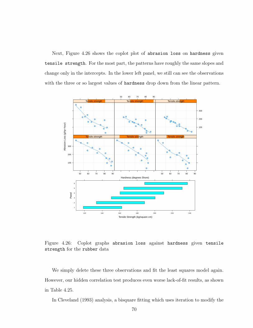
Next, Figure 4.26 shows the coplot plot of abrasion loss on hardness given
tensile strength. For the most part, the patterns have roughly the same slopes and
change only in the intercepts. In the lower left panel, we still can see the observations
with the three or so largest values of hardness drop down from the linear pattern.
Hardness (degrees Shore)
Abr
asio
n Lo
ss (
g/hp
−ho
ur)
100
200
300
50 60 70 80 90
Tensile.strength
Tensile.strength
50 60 70 80 90
Tensile.strength
Tensile.strength
50 60 70 80 90
Tensile.strength
100
200
300
Tensile.strength
Tensile Strength (kg/square cm)
Pan
el
1
2
3
4
5
6
120 140 160 180 200 220 240
Figure 4.26: Coplot graphs abrasion loss against hardness given tensile
strength for the rubber data
We simply delete these three observations and fit the least squares model again.
However, our hidden correlation test produces even worse lack-of-fit results, as shown
in Table 4.25.
In Cleveland (1993) analysis, a bisquare fitting which uses iteration to modify the
70
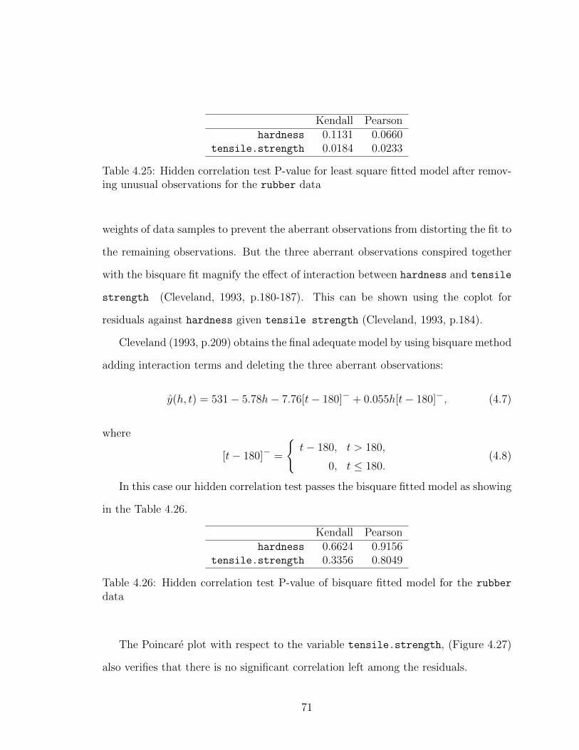
Kendall Pearsonhardness 0.1131 0.0660
tensile.strength 0.0184 0.0233
Table 4.25: Hidden correlation test P-value for least square fitted model after remov-ing unusual observations for the rubber data
weights of data samples to prevent the aberrant observations from distorting the fit to
the remaining observations. But the three aberrant observations conspired together
with the bisquare fit magnify the effect of interaction between hardness and tensile
strength (Cleveland, 1993, p.180-187). This can be shown using the coplot for
residuals against hardness given tensile strength (Cleveland, 1993, p.184).
Cleveland (1993, p.209) obtains the final adequate model by using bisquare method
adding interaction terms and deleting the three aberrant observations:
y(h, t) = 531− 5.78h− 7.76[t− 180]− + 0.055h[t− 180]−, (4.7)
where
[t− 180]− =
t− 180, t > 180,
0, t ≤ 180.(4.8)
In this case our hidden correlation test passes the bisquare fitted model as showing
in the Table 4.26.
Kendall Pearsonhardness 0.6624 0.9156
tensile.strength 0.3356 0.8049
Table 4.26: Hidden correlation test P-value of bisquare fitted model for the rubber
data
The Poincare plot with respect to the variable tensile.strength, (Figure 4.27)
also verifies that there is no significant correlation left among the residuals.
71

−20 0 20 40 60
−20
020
4060
e[t]
e[t+
1]
Figure 4.27: Poincare diagnostic plot for correlation among the residuals of bisquarefitted model for the rubber data
According to our hidden correlation test result the bisquare fitted model is bet-
ter than the usual linear regression model for the rubber dataset since the hidden
correlation test pass. Our diagnostic test also verifies that simply delete the unusual
observations cannot improve the overall fit of the linear regression model.
72

4.10 Windmill Electrical Output and Wind Speed
This dataset was discussed in the paper by Joglekar et al. (1989) and is available in
the dataframe windmill with variables Y and x (Shi and McLeod, 2013). For the
windmill data direct current output, Y , was measured against wind velocity in miles
per hour, x. There were 25 observations recorded. The linear regression model is
highly statistically significant, see Table 4.27, and the adjusted R2 = 89% indicates
the model explains much of the variation.
Estimate Std. Error t value Pr(>|t|)(Intercept) 0.2950 0.4961 0.59 0.5579
x 3.6264 0.2865 12.66 0.0000
Table 4.27: Least square model for the windmill data
Joglekar et al. (1989) considered this dataset for testing nearest-neighbor lack-
of-fit regression diagnostic tests. There were two tests. The first test was based
on the Robillard awarding winning Ph.D. thesis of Richard Shillington. This test
was published in the Canadian Journal of Statistics (Shillington, 1979). The second
was an improved version of the test suggested in the paper (Joglekar et al., 1989).
It was found that these tests both rejected model adequacy at the 1% level. Our
hidden correlation test, Table 4.28, using both Kendall rank test method and Pearson
correlation test method also indicate an inadequate model because the tests results
are statistically significant at 1% level when ordering the residuals according to the
ascending order of the variable x.
Kendall PearsonWind 0.0030 0.0035
Table 4.28: Hidden correlation test P-value of least square fit for the windmill data
73

The Poincare plot of Figure 4.28 also shows a positive correlation in the error
terms.
−1.0 −0.5 0.0 0.5 1.0 1.5
−1.
00.
01.
0
e[t]
e[t+
1]
Figure 4.28: Poincare diagnostic plot for correlation among residuals of least squarefit for the windmill data
Next, a loess model is fitted to the dataset. The hidden correlation test, Table
4.29, does not indicate any correlation among the residuals.
Kendall Pearsonwind 0.5392 0.1676
Table 4.29: Hidden correlation test P-value of loess fit for the windmill data
The Poincare plot of Figure 4.29 also does not show any correlation left in the
residuals for the windmill data.
Our hidden correlation test shows the loess fit is better than the ordinary least
squares fit for the windmill dataset because we removed the correlation among the
residuals. Figure 4.30 comparing the fits also confirms the better fit of the loess
model.
74
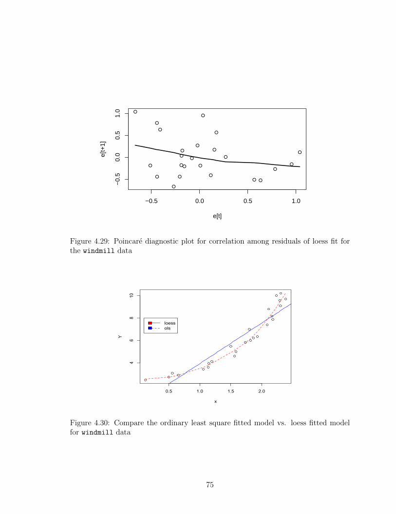
−0.5 0.0 0.5 1.0
−0.
50.
00.
51.
0
e[t]
e[t+
1]
Figure 4.29: Poincare diagnostic plot for correlation among residuals of loess fit forthe windmill data
0.5 1.0 1.5 2.0
46
810
x
Y
loessols
Figure 4.30: Compare the ordinary least square fitted model vs. loess fitted modelfor windmill data
75

4.11 Tensile Strength of Paper
The other dataset in Joglekar et al.’s paper (Joglekar et al., 1989) is the tensile
dataset available in the dataframe tensile (Shi and McLeod, 2013). The tensile
strength of Kraft paper (Y , psi) was measured against the percentage of hardwood in
the batch of pulp from which the paper was produced. There are only 19 observations.
In this case, a quadratic in x is a possible appropriate model (Joglekar et al., 1989).
From the model summary in Table 4.30, excepting the intercept, both predictors are
highly statistically significant and the adjusted R2 = 0.9 also suggests a good model.
Estimate Std. Error t value Pr(>|t|)(Intercept) -6.6742 3.3997 -1.96 0.0673
x 11.7640 1.0028 11.73 0.0000
x2 -0.6345 0.0618 -10.27 0.0000
Table 4.30: Polynomial regression model for the tensile data
However, our hidden correlation test, Table 4.31, in both Kendall rank test method
and Pearson correlation test method suggest an inadequate model since the test results
for the ordered residuals according to the ascending order of the variable hardwood
are statistically significant at 1 % level.
Kendall Pearsonhardwood 0.0264 0.0044
Table 4.31: Hidden correlation test P-value of the polynomial regression model forthe tensile data
The Poincare plot of Figure 4.31 shows the residuals are positive correlated.
The residual dependency plot of Figure 4.32 does not provide such a clear indica-
tion of lack-of-fit.
76

−6 −4 −2 0 2 4 6
−6
−2
02
46
e[t]
e[t+
1]
Figure 4.31: Poincare diagnostic plot for correlation among the residuals of the fittedpolynomial regression model for the tensile data
percentage of hardwood
Res
idua
l for
the
tens
ile s
tren
gth
−5
0
5
5 10 15
Figure 4.32: Residual dependency plot of Residuals vs. hardwood
77

Next a loess model is fitted to the dataset. The hidden correlation test in Table
4.32 does not show any correlation left among the residuals.
Kendall Pearsonhardwood 0.2935 0.3109
Table 4.32: Hidden correlation test P-value of the loess model for the tensile data
The Poincare plot of Figure 4.33 also does not indicate correlation among the
residuals.
−4 −2 0 2 4
−4
−2
02
4
e[t]
e[t+
1]
Figure 4.33: Poincare diagnostic plot for correlation among the residuals of the loessfitted model for the tensile data
Our hidden correlation test indicates the loess fit is better than the ordinary
least squares fit for the tensile dataset since we remove the correlation among the
residuals. Figure 4.34 also indicates the loess fitted model is better than the least
squares fitted model.
78

2 4 6 8 10 12 14
1020
3040
50
x
Y
loesspolynomial
Figure 4.34: Compare the ordinary least square fit model vs. loess fit model
79

4.12 Fisher’s Cat Weight/Heart Data Revisited
The cats dataset was discussed in the paper by Fisher (1947) and is available in the
dataframe cats (Shi and McLeod, 2013). The variables in cats are Sex, Bwt, and
Hwt. The data consist of the body weights in kilograms, Bwt and the heat weights in
grams, Hwt of 144 cats used in a group of digitalis experiment. There were 47 females
and 97 males. In Fisher’s paper he showed the estimated variance of heart weight for
given body weight in males is considerably greater than the value for females. The
greater residuals variance for males possibly was related to their larger size.
Initially, we fit the linear regression model with both predictors, Sex and Bwt
and their interaction term. The model coefficients as provided in Table 4.33 are
statistically significant at 5% level and the usual model diagnostic test does not show
any problem for the fitted least square model.
Estimate Std. Error t value Pr(>|t|)(Intercept) 2.9813 1.8428 1.62 0.1080
SexM -4.1654 2.0618 -2.02 0.0453Bwt 2.6364 0.7759 3.40 0.0009
SexM:Bwt 1.6763 0.8373 2.00 0.0472
Table 4.33: Regression model for the cats data
But our hidden correlation test cannot pass since the test result for the ordered
residuals according to the ascending order of the variable Bwt is highly statistically
significant in both Kendall and Pearson tests as showing in Table 4.34 . So we may
suspect whether the errors are independent among each others.
Kendall Pearson Square.Kendall Square.PearsonBwt 0.0000 0.0142 0.0000 0.0345
Table 4.34: Hidden correlation test P-value of least square fit for the cats data
80

The Poincare plot of Figure 4.35 also indicates a very strong positive dependency
among the ordered residuals.
−4 −3 −2 −1 0 1 2 3
−4
−2
02
4
e[t]
e[t+
1]
Figure 4.35: Poincare diagnostic plot for correlation among the residuals of regressionfor the cats data
The residuals vs predictor, Bwt plot of Figure 4.36 does not provide a clear indi-
cation of lack-of-fit.
From the normal QQ plot and Cook’s distance plot of Figure the case 144 seems
unreasonable so we remove the observation 144 and fit the least squares model again.
However our hidden correlation test result of Table 4.35 still indicates the corre-
lation among the ordered residuals corresponding to the variable Bwt.
Kendall Pearson Square.Kendall Square.PearsonBwt 0.000 0.004 0.000 0.003
Table 4.35: Hidden correlation test P-value for least square fit after removing theoutlier for the cats data
Next we try to use the bisquare robust fitting method.
81

body weight in kg
Res
idua
l Hea
rt W
eigh
t in
g
−4
−2
0
2
4
2.0 2.5 3.0 3.5
Figure 4.36: Residuals dependency plot of Residuals vs. Bwt
−2 0 1 2
−2
01
23
4
Theoretical Quantiles
Sta
ndar
dize
d re
sidu
als
Normal Q−Q
144
140
135
0 40 80 120
0.00
0.05
0.10
0.15
Index
cook
s.di
stan
ce(m
od)
Figure 4.37: Normal QQ plot on the left, Cooks’s distance plot on the right
> rmod<-rlm(Hwt~Sex+Bwt+Sex:Bwt,data=cats,psi=psi.bisquare)
> summary(rmod)
82

Call: rlm(formula = Hwt ~ Sex + Bwt + Sex:Bwt, data = cats, psi = psi.bisquare)
Residuals:
Min 1Q Median 3Q Max
-3.60735 -0.92986 -0.07196 1.04163 5.05132
Coefficients:
Value Std. Error t value
(Intercept) 3.0157 1.8885 1.5968
\textttSexM -3.9729 2.1129 -1.8803
\textttBwt 2.6207 0.7951 3.2959
\textttSexM:Bwt 1.5859 0.8581 1.8482
Residual standard error: 1.417 on 140 degrees of freedom
But our hidden correlation test still can detect the correlation among the residuals
corresponding to the same variable Bwt as illustrative in Table 4.36.
Kendall Pearson Square.Kendall Square.PearsonBwt 0.0000 0.0136 0.0000 0.0323
Table 4.36: Hidden correlation test P-value of the bisquare fit for the cats data
In later research, we plan to investigate using regression splines as a simple method
to overcome the lack-of-fit. Regression splines provides a more flexible and better
approach than polynomial regression Hastie et al. (2009).
83

4.13 Ozone Pollution in Los Angeles
The ozone dataset comes from a study of the relationship between atmospheric ozone
concentration, O3 and other meteorological variables in the Log Angeles Basin in
1976 with n = 330 and p = 9. The data is available in the dataframe ozone (Shi and
McLeod, 2013). The variables in this dataframe are O3, vh, wind, humidity, temp,
ibh, dpg, ibt, vis, and doy. These variables are described in more detail in the the
documentation for ozone (Shi and McLeod, 2013).
The data was first presented by Breiman and Friedman (1985). Initially a lin-
ear regression model is fitted to this dataset with all insignificant terms removed as
showing in Table 4.37.
Estimate Std. Error t value Pr(>|t|)(Intercept) -10.0179 1.6531 -6.06 0.0000
vis -0.0082 0.0037 -2.22 0.0270doy -0.0102 0.0024 -4.17 0.0000ibt 0.0349 0.0067 5.21 0.0000
humidity 0.0851 0.0143 5.93 0.0000temp 0.2328 0.0361 6.45 0.0000
Table 4.37: Regression model for the ozone data
Our hidden correlation test in both Kendall rank test method and Pearson corre-
lation test method confirm that a usual linear model is not adequate. Because when
we order the residuals according to the ascending order of the variable doy or ibt, the
P-values of both test statistics are extremely small, which suggest a strong correlation
among the residuals as can be seen in Table 4.38.
The resulting Poincare plot of Figure 4.38 also confirms the correlation among
residuals corresponding to the ordered doy variable. But the usual residual depen-
dence plots does not clearly indicate lack-of-fit.
84

Kendall Pearsonhumidity 0.4591 0.8654
temp 0.2876 0.1867ibt 0.0005 0.0015vis 0.0967 0.5705doy 0.0000 0.0000
Table 4.38: Hidden correlation test P-value of the least square fit for ozone data
−10 −5 0 5 10
−10
−5
05
10
e[t]
e[t+
1]
Figure 4.38: Poincare diagnostic plot with respect to doy for correlation among resid-uals of least square fit for Ozone data
We use an additive model with the R core package Hastie (2013) to fit a model
to the inputs used in Table 4.37. After several iterations, experimenting with the
smoothing, a model is found that works.
> require("hcc")
> require("gam")
> data(ozone)
> ans <- gam(O3 ~ humidity+temp+vis+
+ lo(ibt,degree=2, span=0.5) + lo(doy, span=0.25, degree=2),
+ data=ozone)
> ans
85

Call:
gam(formula = O3 ~ humidity + temp + vis + lo(ibt, degree = 2,
span = 0.5) + lo(doy, span = 0.25, degree = 2), data = ozone)
Degrees of Freedom: 329 total; 307.4586 Residual
Residual Deviance: 5037.608
> res<-resid(ans)
> hctest(ozone$ibt, res)
[1] 0.07780387
> hctest(ozone$doy, res)
[1] 0.05199917
This model works since the hidden correlation test results are statistically signifi-
cant at 5 % level.
86

Conclusion
Chapter 5
Conclusion
5.1 Conclusion
We investigated the test for hidden correlation on many datasets that have been
previously investigated by others. In some cases such as with the datasets trees in
§4.2, ustemp in §4.6, gala in §4.7, and rubber in §4.9 our test performed as well as
other methods in choosing the model.
In other cases, we found flaws in the existing models that seem to have been
previously undetected as with birthwt data in §4.4 and dicentric data in §4.5.
Work is currently underway to develop improved models.
Using the new test we suggested an improved model for the beam dataset in §4.8,
using regression by adding a square term to one of the covariates. Similarly we found
that a loess fit is better than the usual least square fit for the tensile dataset in
§4.11, a generalized additive model provides a better alternative to regression for the
Los Angeles ozone data, ozone in §4.13.
We investigated many other datasets as well but have only reported on some
representative interesting ones due to space limitations.
Methods that have been found helpful in dealing with lack-of-fit detecting by our
hidden correlation test include splines, local polynomials, multi-adaptive regression
splines or MARS, and generalized additive models.
The hidden correlation problem was motivated by generalizing the concept of
spurious regression that is caused by correlation of observations close together in time
series regression to non-time series regression problems. We now understand that the
87

resulting test is related to nearest-neighbor lack-of-fit tests discussed by Shillington
(1979); Joglekar et al. (1989).
88

Bibliography
H. Abdi. Kendall rank correlation. Encyclopedia of Measurement and Statistics, pages
508–510, 2007.
B. Abraham and J. Ledolter. Introduction to Regression Modeling. Brooks/Cole,
2006.
AC. Atkinson. Plots, Transformations and Regression. Oxford, 1985.
G. E. P. Box and D. R. Cox. An analysis of transformations. Journal of the Royal
Statistical Society B, 26:211–252, 1964.
G. E. P. Box and N. R. Draper. Empirical Model-Building and Response Surfaces.
Wiley, 1987.
G. E. P. Box and P. Newbold. Some comments on a paper of coen, gomme and
kendall. Journal of the Royal Statistical Society, A 134:229–240, 1971.
Michael Brennan, Marimuththu Palaniswami, and Peter W. Kamen. Do existing mea-
sures of poincare plot geometry reflect nonlinear features of heart rate variability?
IEEE Transactions on Biomedical Engineering, 48:1342–1347, 2001.
M Buyse, S L George, S Evans, N L Geller, J Ranstam, B Scherrer, E Lesaffre,
G Murray, L Edler, J Hutton, and et al. The role of biostatistics in the prevention,
detection and treatment of fraud in clinical trials. Statistics in Medicine, 18(24):
3435–51, 1999. URL http://www.ncbi.nlm.nih.gov/pubmed/10611617.
89

W. S Cleveland. Robust locally weighted regression and smoothing scatter plots.
Journal of the American Statistical Association, 74:829–836, 1979.
W. S. Cleveland. Visualizing Data. Hobart Press, 1993.
N. R. Draper and D. M. Stoneman. Testing for the inclusion of variables in linear
regression by a randomisation technique. American Statistical Association, 8:695–
699, 1966.
J. Faraway. Linear Models with R. Chapman & Hall/CRC, 2005.
J. Faraway. Extending the linear model with R. Chapman & Hall/CRC, 2006.
R. A. Fisher. The analysis of covariance methods for the relation between a part and
the whole. American Statistical Association the Biometrics Section, 3:65–68, 1947.
A. Franklin. Ending the Mendel-Fisher Controversy. University of Pittsburgh Press,
2008.
C. W. J. Granger and P. Newbold. Essays in econometrics. chap-
ter Spurious regressions in econometrics, pages 109–118. Harvard Univer-
sity Press, Cambridge, MA, USA, 2001. ISBN 0-521-79697-0. URL
http://dl.acm.org/citation.cfm?id=781840.781846.
T. Hastie, R. Tibshirani, and J. H. Friedman. The Elements of Statistical Learning:
Data Mining, Inference and Prediction. Springer-Verlag, New York, 2nd edition,
2009.
T. J. Hastie and R. J. Tibshirani. Generalized Aditive Models. Chapman & Hall,
1990.
90

Trevor Hastie. gam: Generalized Additive Models, 2013. URL http://CRAN.R-
project.org/package=gam. R package version 1.06.2. Access date: 2013-03-26.
G. Joglekar, J. H. Schuenemeyer, and V. LaRiccia. Lack of fit testing when replicates
are not available. The American Statistician, 43:135–143, 1989.
M. P. Johnson and P. H. Raven. Species number and endemism: The galapagos
archipelago revisited. Science, 179:893–895, 1973.
Esam Mahdi. Diagnostic Checking, Time Series and Regression. PhD thesis, Univer-
sity of Western Ontario, 2011. URL http://ir.lib.uwo.ca/etd/244.
A. I. McLeod and W. K. Li. Diagnostic checking ARMA time series models using
squared-residual autocorrelations. Journal of Time Series Analysis, 4:269–273,
1983.
A. I. McLeod and Yun Shi. Hidden Correlation in Regression, 2013. URL
http://demonstrations.wolfram.com/HiddenCorrelationInRegression/.
Wolfram Demonstrations Project.
J. W. Neill and D. E. Johnson. Testing for lack of fit in regression - a review. Com-
munications in Statistics A: Theory and Methods, 13:485–511, 1984.
J. L. Peixoto. A property of well-formulated polynomial regression models. The
American Statistician, 44:26–30, 1990.
R Development Core Team. R: A Language and Environment for Statistical Com-
puting. R Foundation for Statistical Computing, Vienna, Austria, 2013. URL
http://www.R-project.org. ISBN 3-900051-07-0.
J. L. Rodgers and W. A. Nicewander. Thirteen ways to look at the correlation
coefficient. American Statistical Association, 42:59–66, 1988.
91

T. A. Ryan, B. L. Joiner, and B. F. Ryan. The Minitab Student Handbook. Duxbury
Press, 1976.
A. Sen and M. Srivastava. Regression Analysis: Theory, Methods, and Applications.
Springer, 1990.
S. J. Sheather. A Modern Approach to Regression with R. Springer, 2009.
Yun Shi and A. I. McLeod. hcc: Hidden correlation check, 2013. URL
http://CRAN.R-project.org/package=hcc. R package version 0.6. Access date:
2013-03-26.
E. Richard Shillington. Testing lack of fit in regression without replica-
tion. The Canadian Journal of Statistics, 7(2):pp. 137–146, 1979. URL
http://www.jstor.org/stable/3315113.
S. Siegel. Nonparametric statistics. The American Association, 11:13–19, 1957.
Howell Tong. Non-linear Time Series: A Dynamical System Approach. Oxford, 1990.
R. S. Tsay. Analysis of Financial Time Series. Wiley, New York, 3rd edition, 2010.
2nd edition, 2005.
W. N. Venables and B. Ripley. Modern applied Statistics with S. Springer, 2002.
C. Weir and G. Murray. Fraud in clinical trials. Significance, 2011. doi:
10.1111/j.1740-9713.2011.00521.x.
S. Weisberg. Applied Linear Regression. Wiley, 1985.
S. N. Wood. Generalized Additive Models: An Introduction with R. Chapman &
Hall/CRC, 2006.
92

Simon Wood. mgcv: Mixed GAM Computation Vehicle with GCV/AIC/REML
smoothness estimation, 2012. URL http://CRAN.R-project.org/package=hcc.
R package version 1.7-22. Access date: 2013-03-26.
93

Curriculum Vitae
Name: Yun Shi
Post-Secondary Beijing Business and Technology University
Education and Beijing, China
Degrees: 2007-2011 Bachelor of Arts
Western University
London, Ontario
2011 - 2013 Master of Science
Honours and National University Student Scholarship in China
Awards: 2009-2010
Related Work Teaching Assistant
Experience: Western University
2011- 2013
94
Recommended