LUND UNIVERSITY
PO Box 117221 00 Lund+46 46-222 00 00
A Least-Squares Fitting Technique for Spectral Analysis of Direct and Frequency-Modulation Lineshapes.
Avetisov, Slava
Published: 1995-01-01
Link to publication
Citation for published version (APA):Avetisov, S. (1995). A Least-Squares Fitting Technique for Spectral Analysis of Direct and Frequency-Modulation Lineshapes. (Lund Reports in Atomic Physics; Vol. LRAP-186). Atomic Physics, Department ofPhysics, Lund University.
General rightsCopyright and moral rights for the publications made accessible in the public portal are retained by the authorsand/or other copyright owners and it is a condition of accessing publications that users recognise and abide by thelegal requirements associated with these rights.
• Users may download and print one copy of any publication from the public portal for the purpose of privatestudy or research. • You may not further distribute the material or use it for any profit-making activity or commercial gain • You may freely distribute the URL identifying the publication in the public portal

Take down policyIf you believe that this document breaches copyright please contact us providing details, and we will removeaccess to the work immediately and investigate your claim.
Download date: 14. Jun. 2018

A Least-Squares Fitting Technique
for Spectral Analysis of
Direct and Frequency-Modulation Lineshapes
Viacheslav G. Avetisov
LRAP-186
Lund Reports on Atomic Physics
1995

A Least-Squares Fitting Technique for Spectral Analysis of Direct and Frequency-Modulation Lineshapes
Viacheslav G. Avetisov
Division of Atomic Physics, Lund Institute of Technology
P.O. Box 118, S-221 00 Lund, Sweden
Abstract
A nonlinear least-squares fitting procedure has been developed to model direct absorption
and two-tone frequency-modulation lineshapes using the Voigt, Galatry and Rautian
Sobelman profiles. Details for the lineshape calculations are presented and the iterative
least-squares fitting procedure based on the Levenberg-Marquardt method is described.
1. Introduction
A nonlinear least-squares fitting technique is generally employed to determine
spectroscopic parameters from high-resolution spectra. The basic approach in all cases is
usually the same: a model function with a particular choice of parameters is chosen that is
supposed to give the best agreement with data. These parameters are then adjusted using
an iterative procedure to minimise the sum of the squares of the differences between
observed spectrum and calculated spectrum. This yields the best-fit parameters. For a
given experimental spectrum the procedure fits positions, intensities, widths and and/or
other parameters of the spectral lines.
In a variety of spectroscopic applications there is a need for quantitative
measurements of gas parameters such as concentration, temperature, total pressure, and
mixing ratios of molecular and atomic species. In this case, the least-squares fitting
technique assumes knowledge of the spectral line parameters, such as line strengths and
pressure broadening coefficients to derive the gas parameters.
Two-tone frequency modulation spectroscopy (TTFMS) is a promising technique
for gas analysis in industrial and environmental applications. The ability to extract spectral
information from TTFMS lineshapes in combination with high sensitivity of the technique
2
is especially important in the case of measurements in a highly varying environment (e.g.
combustion), where variations of the linewidth are significant
Analytical expressions required for calculations of the spectral profiles and their
derivatives are given in Section 2. The analysis is based on the literature and is applicable
for both absorption and emission lineshapes. In Section 3 spectral calculations of TTFMS
lineshapes are described. Section 4 provides a survey of the very powerful Levenberg
Marquardt method, which today is often used in nonlinear least-squares fitting routines.
Section 5 describes the program for spectral calculations and modelling of lineshapes
recorded using direct detection and TTFMS.
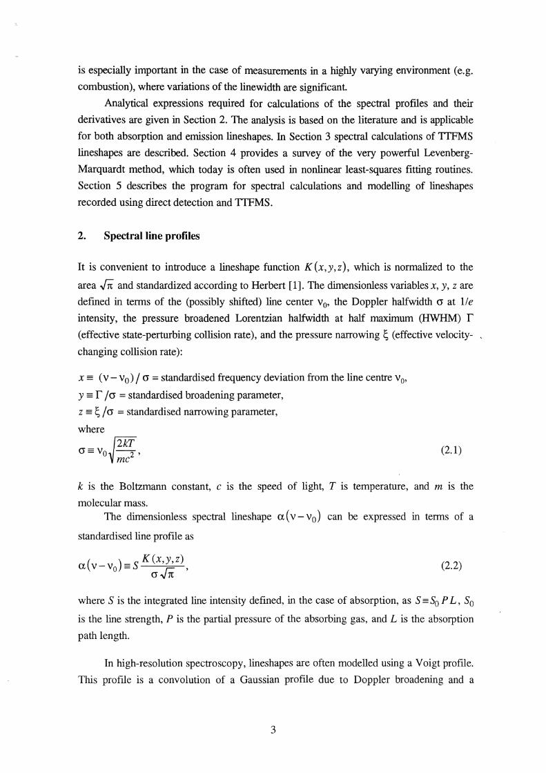
2. Spectral line profiles
It is convenient to introduce a lineshape function K(x,y,z), which is normalized to the
area ..fit and standardized according to Herbert [1]. The dimensionless variables x, y, z are
defmed in terms of the (possibly shifted) line center v0, the Doppler halfwidth a at 11 e
intensity, the pressure broadened Lorentzian halfwidth at half maximum (HWHM) r (effective state-perturbing collision rate), and the pressure narrowing~ (effective velocity- ,
changing collision rate):
x = (v- v0 ) J a= standardised frequency deviation from the line centre v0,
y = r ja =standardised broadening parameter,
z =~fa =standardised narrowing parameter,
where
a=vo~2k;' me
(2.1)
k is the Boltzmann constant, c is the speed of light, T is temperature, and m is the
molecular mass. The dimensionless spectral lineshape a ( v - v0) can be expressed in terms of a
standardised line profile as
( ) _SK(x,y,z) a v-v0 = c ,
a'\11t (2.2)
where S is the integrated line intensity defined, in the case of absorption, as S = S0 P L, S0
is the line strength, P is the partial pressure of the absorbing gas, and L is the absorption
path length.
In high-resolution spectroscopy, lineshapes are often modelled using a Voigt profile.
This profile is a convolution of a Gaussian profile due to Doppler broadening and a
3
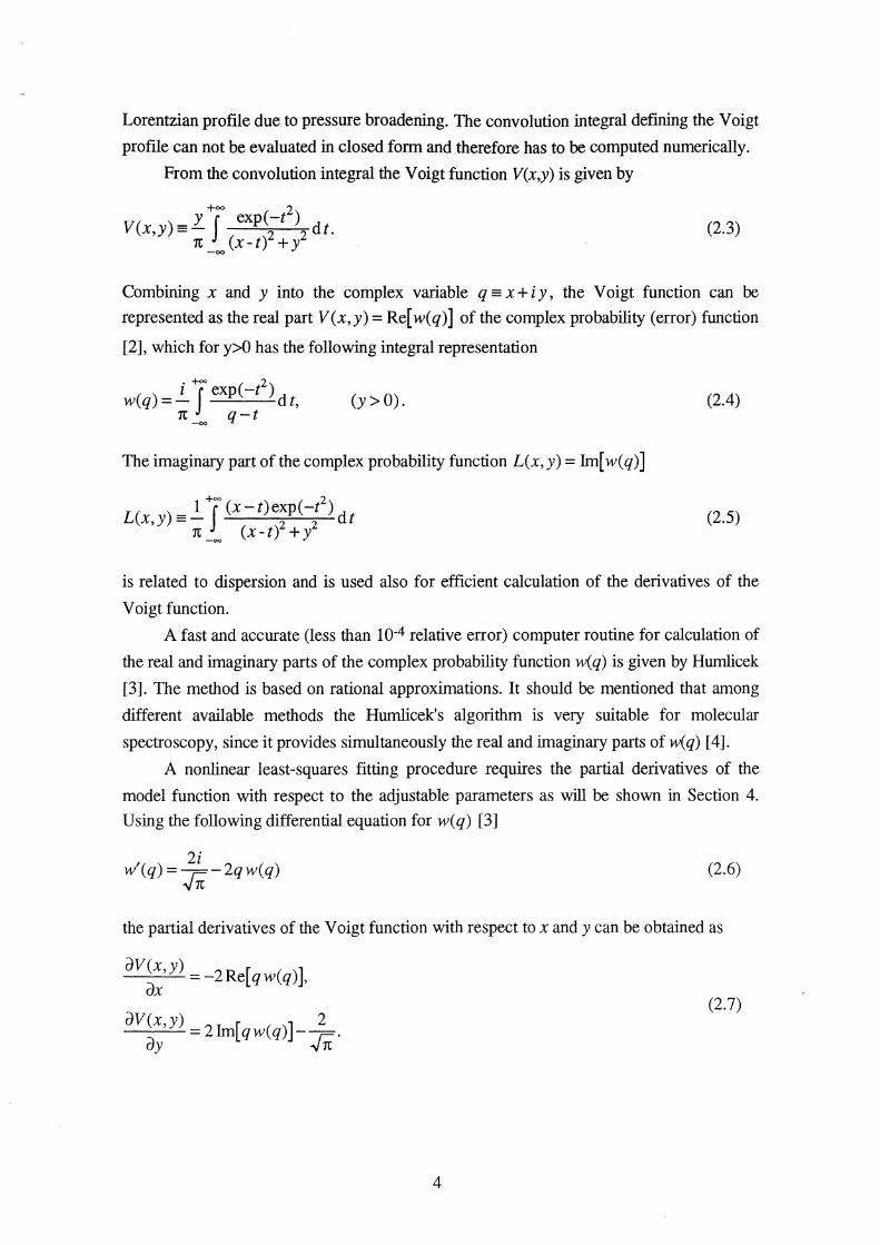
Lorentzian profile due to pressure broadening. The convolution integral defining the Voigt
profile can not be evaluated in closed form and therefore has to be computed numerically.
From the convolution integral the Voigt function V(x,y) is given by
+oo 2 V(x,y)=ZJ exp(-t) dt.
1t (x-t)2+i -oo
(2.3)
Combining x and y into the complex variable q = x + i y , the Voigt function can be
represented as the real part V(x,y) = Re[ w(q)] of the complex probability (error) function
[2], which for y>O has the following integral representation
w(q) = j_ +Joo exp( -!2) d t, 1t -oo q- (
(y > 0).
The imaginary part of the complex probability function L(x,y) = Im[w(q)]
+oo 2 L(x,y) =_!_ J (x-t)exp(-t ) dt
1t_00 (x-t)2 +/
(2.4)
(2.5)
is related to dispersion and is used also for efficient calculation of the derivatives of the
Voigt function.
A fast and accurate (less than I0-4 relative error) computer routine for calculation of
the real and imaginary parts of the complex probability function w(q) is given by Humlicek
[3]. The method is based on rational approximations. It should be mentioned that among
different available methods the Humlicek's algorithm is very suitable for molecular
spectroscopy, since it provides simultaneously the real and imaginary parts of w(q) [ 4].
A nonlinear least-squares fitting procedure requires the partial derivatives of the
model function with respect to the adjustable parameters as will be shown in Section 4.
Using the following differential equation for w(q) [3]
2i w'(q)= Jn-2qw(q) (2.6)
the partial derivatives of the Voigt function with respect to x and y can be obtained as
oV(x,y) 2R [ ( )] ax =- e qw q '
oV(x,y) = 2Im[qw(q)]-~. ay Jn
(2.7)
4
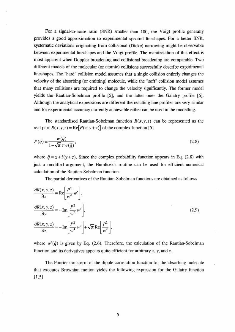
For a signal-to-noise ratio (SNR) smaller than 100, the Voigt profile generally
provides a good approximation to experimental spectrallineshapes. For a better SNR,
systematic deviations originating from collisional (Dicke) narrowing might be observable
between experimentallineshapes and the Voigt profile. The manifestation of this effect is
most apparent when Doppler broadening and collisional broadening are comparable. Two
different models of the molecular (or atomic) collisions successfully describe experimental
lineshapes. The "hard" collision model assumes that a single collision entirely changes the
velocity of the absorbing (or emitting) molecule, while the "soft" collision model assumes
that many collisions are required to change the velocity significantly. The former model
yields the Rautian-Sobelman profile [5], and the latter one- the Galatry profile [6].
Although the analytical expressions are different the resulting line profiles are very similar
and for experimental accuracy currently achievable either can be used in the modelling.
The standardised Rautian-Sobelman function R(x,y,z) can be represented as the
real part R(x,y,z) = Re[P(x,y+ z)] of the complex function [5]
P(-) = w(q) q -1 c (-)' -'\11t zw q
(2.8)
where q=x+i(y+z). Since the complex probability function appears in Eq. (2.8) with
just a modified argument, the Humlicek's routine can be used for efficient numerical
calculation of the Rautian-Sobelman function.
The partial derivatives of the Rautian-Sobelman functions are obtained as follows
CJR(x,y,z) = R [P2 '] a e 2 w ,
X W
CJR(x,y,z) =-Im[p2 w'] CJy w2 '
(2.9)
CJR(x,y,z) =-Im[p2 w']+..fitRe[p2], az w4 w2
where w'(q) is given by Eq. (2.6). Therefore, the calculation of the Rautian-Sobelman
function and its derivatives appears quite efficient for arbitrary x, y, and z.
The Fourier transform of the dipole correlation function for the absorbing molecule
that executes Brownian motion yields the following expression for the Galatry function
[1,5]
5

(2.10)
Using the relation of the Galatry function to the incomplete gamma function,
Herbert [1] presented several approximate expressions that, depending on the values of y
and z, can be implemented to calculate the Galatry function. For each expression the
region of x, y, and z values as well as the number of terms required for 10-4 relative error
were determined by Varghese and Hanson [7].
The first expression is an asymptotic expansion around the Voigt function, and it can
be used for small x, y, and z,
G(x,y,z) = Re w(q)+ L ~~ -n w(q) , [ nr dn ]
n=3 l dq
(2.11)
where
; ~ 2 c7 =--+c3 ·c4 c8 =---+c3 ·c5 +Yzc4 •
2·7! ' 2·8!
(2.12)
The derivatives of w(q) may be obtained by the following recursion relation for n ~ 2
dn [ dn-1 dn-2 l -n w(q) = -2 q-n::rw(q) + (n -1)-----rz=2w(q) , dq dq dq
(2.13)
and by Eq. (2.6) for n=1.
The second expression is based on a series expansion of the incomplete gamma
function, which can be used for relatively large values of z,
G(x,y,z) = 2~ Re{~ 1 ] ]}' -v rr n=0 [1 + 2z(y- ix)][1 + 2z(y- ix + z) · · ·[1 + 2z(y- ix + nz)
n2 = 4+z-1.05 [1+3exp(-1.1y)], (2.14)
( < 4 0.87 > 0 1) y_ z , z_ ..
6

The third expression is based on an approximation of the incomplete ganuna
function by using a continued fraction, and it can be used for relatively large values of y.
G(x,y,z)= JnRefy-it+ 1 ~-~ z-~ 1·
z+y-zx+ 2 2z+y-ix+···
n3 =2+37exp(-0.6y), (2.15)
(y > 1, 0.4 < z < 0.1) and (y > 4z0·87 , z > 0.1).
The partial derivatives of the Galatry function can be obtained numerically by calculating
divided differences.
In modelling spectrallineshapes the following parameters are adjustable: v0, S, y,
and z. It is important to provide the fitting procedure with good initial values of these
parameters. The Doppler halfwidth is calculated from the temperature and absolute
wavelength of the transition. The initial value of the line center v0 can be easily obtained
from the position of the lineshape maximum. The parameter z is generally not very
decisive in forming the lineshape and can be set to zero. To provide the initial value of the
broadening parameter y the lineshape is assumed to be the Voigt. Various empirical
expressions exist for the width of the Voigt profile [8]. A very simple and accurate
approximation (better than 0.01 relative error over the whole range of y) was given by
Whiting [9]:
xv2 = y /2 + ~ y 2/ 4 + ln 2 , (2.16)
where xl/2 is the standardised Voigt (HWHM). Using this expression the initial value of
the broadening parameter can be estimated from the measured HWHM as
(2.17)
In order to determine the initial value of the integrated line intensity S, a Voigt lineshape
can be fitted to the experimentallineshape by using the obtained initial values of v0 andy,
which are fixed. In the subsequent nonlinear least-squares fitting any of the profiles can be
used. It might be useful to perform the first iteration with a Voigt profile, which provides
good starting values for the next iteration with a collisionally narrowed profile.
7
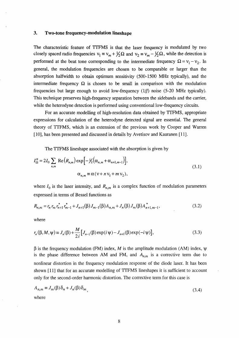
3. Two-tone frequency-modulation lineshape
The characteristic feature of TTFMS is that the laser frequency is modulated by two
closely spaced radio frequencies v1 = v m + X Q and v2 = v m - X Q, while the detection is
performed at the beat tone corresponding to the intermediate frequency Q = v1 -v2 . In
general, the modulation frequencies are chosen to be comparable or larger than the
absorption halfwidth to obtain optimum sensitivity (500-1500 MHz typically), and the
intermediate frequency Q is chosen to be small in comparison with the modulation
frequencies but large enough to avoid low-frequency (1/J) noise (5-20 MHz typically).
This technique preserves high-frequency separation between the sidebands and the carrier,
while the heterodyne detection is performed using conventional low-frequency circuits.
For an accurate modelling of high-resolution data obtained by TTFMS, appropriate
expressions for calculation of the heterodyne detected signal are essential. The general
theory of TTFMS, which is an extension of the previous work by Cooper and Warren
[ 10], has been presented and discussed in details by A vetisov and Kauranen [ 11].
The TTFMS lineshape associated with the absorption is given by
I~= 2/o L Re(Rn,m) exp[-Yz(an,m +an+l,m-1)]. n,m (3.1)
where / 0 is the laser intensity, and Rn,m is a complex function of modulation parameters
expressed in terms of Bessel functions as
(3.2)
where
(3.3)
~ is the frequency modulation (FM) index, M is the amplitude modulation (AM) index, \jf is the phase difference between AM and FM, and An,m is a corrective term due to
nonlinear distortion in the frequency modulation response of the diode laser. It has been
shown [11] that for an accurate modelling of TTFMS lineshapes it is sufficient to account
only for the second-order harmonic distortion. The corrective term for this case is
(3.4)
where
8

(3.5)
~ and t} are the second-harmonic amplitude and phase shift, respectively.
For the expression (3.1) to be accurate with I0-3 relative error the following
requirements were obtained
Q 3 Q a(v0)-<4x10-, -<0.2,
~ ~ (3.6)
which are generally fulfilled in practice.
The expressions presented above can be simplified by applying the approximation v 1
-;::;;y2-;::;;vm. The TTFMS lineshape is then represented as
Ig = 2/o L Re(Rn,m) exp{ -a[v+ (n+m) vm] }, (3.7) n,m
where
(3.8)
The expression (3. 7) is accurate with I0-3 relative error if
(3.9)
The maximum values of n and m required for the calculation of the lineshape by Eq s.
(3.1) and (3.7) with a I0-3 relative error can be determined for moderate FM indices(~
<1.5) using the following empirical relations:
lnl~4, lml~4, lnl+lml~2+2.3~. (3.10)
For simplicity, the de offset c£0 E(f M 2 due to the AM is eliminated in the
calculated lineshapes by subtraction. The absorption of a sideband at frequency v c + n v1 + m v2 is computed according to
(3.11)
where v1 =vi jcr and v2 = v2 jcr. When using Eq. (3.7) one approximates
n v1 + m\!2 ::: (n+ m)vw where vm = vm jcr. Thus, five modulation parameters ~, M, 'Jf,
\\ and v2 and five spectroscopic parameters S, y, z, v0 and cr determine a TTFMS
lineshape. Normally, the values of cr, vi, and v2 (or vm) are well known, and it was
9

shown [ 11] that setting 'lf=1t/2 is generally a good approximation. The phase shift of the
harmonic distortion is generally '(}=n in diode lasers [12] and can be fixed, while the
amplitude s might be either set manually or adjusted in the final iteration (typically s =0.01-0.03). Thus, the principal parameters to be adjusted areS, y, z, Y0, ~'and M.
The partial derivatives with respect to S, y, z, v0 are easily obtained by multiplying
each term in Eq. (3.1) or (3.7) to the corresponding derivative ofthe lineshape function
dK(x+n\11 +mv2,y,z)
dai
where ai is either the S, y, z, and Yo parameters. The Bessel functions are computed using
the recurrence formula
(3.12)
and the derivatives of the Bessel functions required in the least-squares fitting procedure
for adjusting the FM index ~ are calculated as
(3.13)
The partial derivative of Rn m with respect to ~ and M are computed according to ,
(3.14)
where aj is either~ or M.
The initial value for the FM index can be estimated experimentally e.g. from the
relative ratio of the sidebands and the carrier component obtained from a spectrum of
direct transmission of a high-finesse Fabry-Perot etalon. The amplitude of the k-ht.
sideband component (k=O for the carrier component) is given by
(3.15) n
Table 1 lists the peak amplitude ratio of four successive sidebands to the carrier
component as a function of the FM index ~' which might be of help when estimating ~.
10

Table 1. The sideband-to-carrier ratio in the Fabry-Perot transmission spectrum as a
function of the FM index~ calculated using Eq. (3.15) with M=O and ~=0.
~ 1tf1o 1zJlo 13/10 14/1o
0.1 0.005 0 0 0
0.2 0.020 0.0002 0 0
0.3 0.046 0.0008 0 0
0.4 0.083 0.0026 0 0
0.5 0.132 0.0065 0.0002 0
0.6 0.194 0.014 0.0005 0
0.7 0.270 0.027 0.0013 0
0.8 0.357 0.049 0.003 0.0001
0.9 0.454 0.081 0.007 0.0003
1.0 0.555 0.127 0.013 0.0008
1.1 0.648 0.187 0.024 0.002
1.2 0.722 0.260 0.042 0.004
1.3 0.763 0.338 0.066 0.007
1.4 0.767 0.413 0.096 0.012
1.5 0.735 0.475 0.133 0.020
1.6 0.679 0.519 0.172 0.030
1.7 0.613 0.543 0.213 0.043
1.8 0.552 0.549 0.254 0.060
1.9 0.503 0.543 0.295 0.080
2.0 0.471 0.527 0.334 0.105
The initial value of the AM index can be set to zero [ 11]. An estimation of the
broadening parameter is not so straightforward. If the FM index is estimated, an arbitrary
guess of y can be used in the first iteration with the Voigt profile. More accurately, the
Voigt HWHM can be estimated from a TTFMS lineshape using the empirical expression
(3.16)
where ~x is the standardised distance between the two minima of the TTFMS lineshape.
The expression provides a better than 10% estimate of the HWHM for v m :::; 2 and
~ :::; 1. 2. Then the broadening parameter can be calculated by Eq. (2.17). The initial value
of the line center v0 is provided by the position of the lineshape maximum, and the
parameter z can be initially set to zero.
11
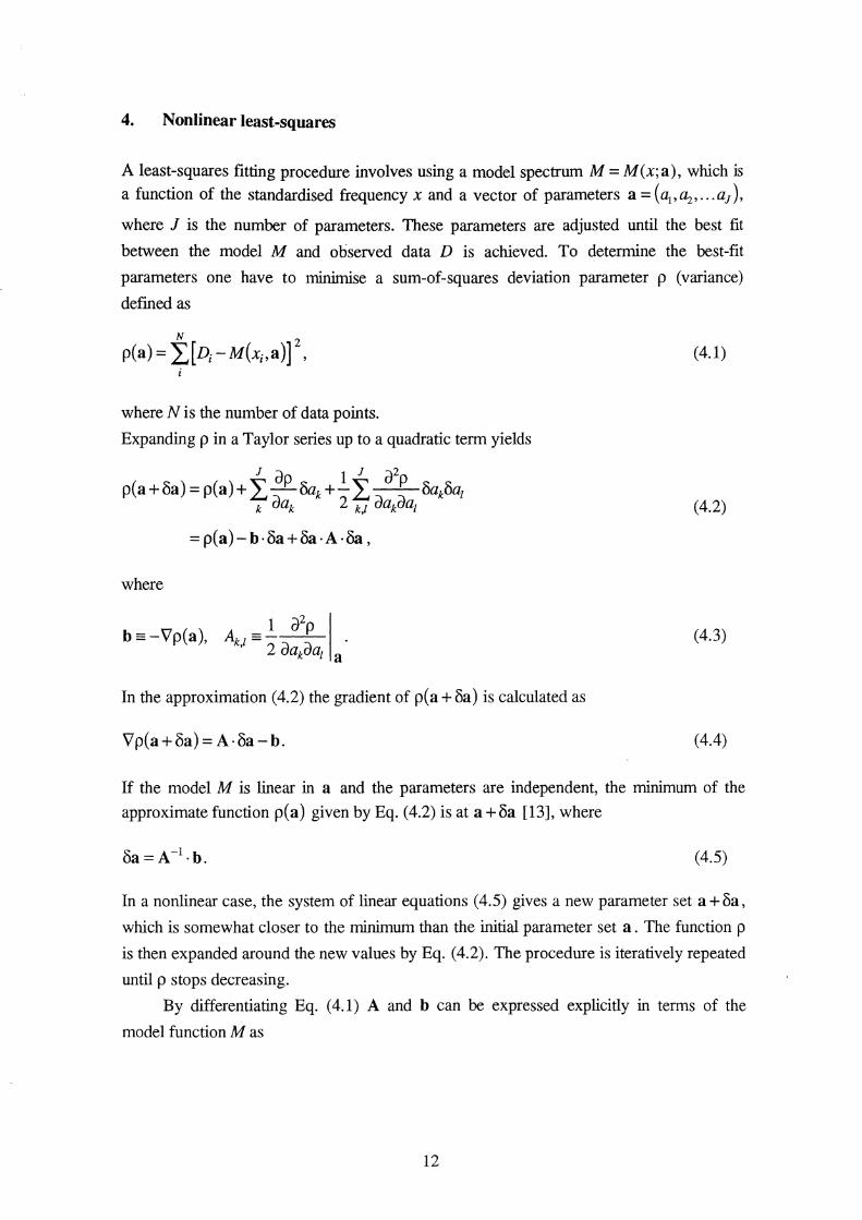
4. Nonlinear least-squares
A least-squares fitting procedure involves using a model spectrum M = M(x;a), which is a function of the standardised frequency x and a vector of parameters a = ( llt, ~, ... a 1 ),
where J is the number of parameters. These parameters are adjusted until the best fit
between the model M and observed data D is achieved. To determine the best-fit
parameters one have to minimise a sum-of-squares deviation parameter p (variance)
defmed as
N 2 p(a) = L,[ni- M(xi,a)] , (4.1)
I
where N is the number of data points.
Expanding p in a Taylor series up to a quadratic term yields
1 o 1 1 o2 p(a+8a)=p(a)+ L, _e_8ak+-L, p 8ak8a1
k aak 2 k,l aakaal (4.2)
= p(a)- b·8a+8a·A·8a,
where
b=-Vp(a), (4.3)
In the approximation (4.2) the gradient of p(a + 8a) is calculated as
Vp(a+8a) = A·8a-b. (4.4)
If the model M is linear in a and the parameters are independent, the minimum of the
approximate function p(a) given by Eq. (4.2) is at a+ 8a [13], where
(4.5)
In a nonlinear case, the system of linear equations ( 4.5) gives a new parameter set a+ 8a,
which is somewhat closer to the minimum than the initial parameter set a . The function p
is then expanded around the new values by Eq. (4.2). The procedure is iteratively repeated
until p stops decreasing.
By differentiating Eq. (4.1) A and b can be expressed explicitly in terms of the
model function M as
12
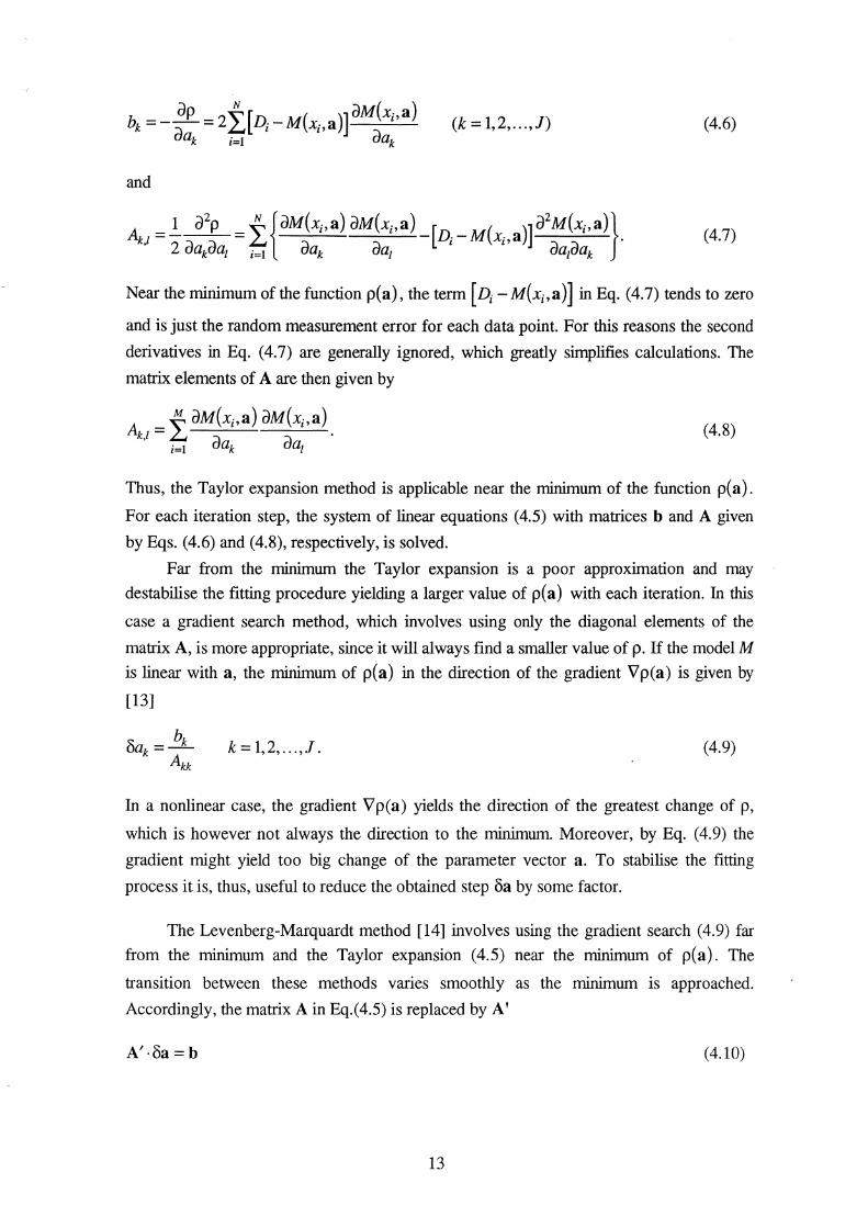
(k = 1,2, ... ,J) (4.6)
and
(4.7)
Near the minimum of the function p{a), the term [ Di- M(x;,a)] in Eq. (4.7) tends to zero
and is just the random measurement error for each data point. For this reasons the second
derivatives in Eq. ( 4. 7) are generally ignored, which greatly simplifies calculations. The
matrix elements of A are then given by
A _ ~ dM(xi,a) aM(xi,a) kl- L.. .
' i=I dak daz (4.8)
Thus, the Taylor expansion method is applicable near the minimum of the function p{a).
For each iteration step, the system of linear equations ( 4.5) with matrices b and A given
by Eqs. (4.6) and (4.8), respectively, is solved.
Far from the minimum the Taylor expansion is a poor approximation and may
destabilise the fitting procedure yielding a larger value of p{ a) with each iteration. In this
case a gradient search method, which involves using only the diagonal elements of the
matrix A, is more appropriate, since it will always find a smaller value of p. If the model M
is linear with a, the minimum of p{a) in the direction of the gradient Vp(a) is given by
[13]
k = 1,2, ... ,J. (4.9)
In a nonlinear case, the gradient Vp(a) yields the direction of the greatest change of p,
which is however not always the direction to the minimum. Moreover, by Eq. (4.9) the
gradient might yield too big change of the parameter vector a. To stabilise the fitting
process it is, thus, useful to reduce the obtained step oa by some factor.
The Levenberg-Marquardt method [14] involves using the gradient search (4.9) far
from the minimum and the Taylor expansion (4.5) near the minimum of p{a). The
transition between these methods varies smoothly as the minimum is approached.
Accordingly, the matrix A in Eq.(4.5) is replaced by A'
A'·Ba =b (4.10)
13

which is given by
(4.11)
For large values of 'A, the matrix A' is constrained to be diagonal, which means that the
method is identical to the gradient search [Eq.(4.9)] except the step size is reduced by the
factor 1/(1 +'A). For 'A<<l, A'=A and the method is identical to the Taylor expansion.
The fitting process can be started using e.g. 'A=O.Ol. When the set of linear equations
( 4.10) is solved and p( a+ oa) is evaluated, 'A is either multiplied or divided by a factor
(e.g. 10) depending on whether p(a + oa) appears to be larger or smaller than p(a).
The method has proven itself as very flexible, fast and reliable, and has become
commonly used in nonlinear least-squares procedures.
5. The program structure
The program for spectral analysis is written using Turbo-Pascal for the MS-DOS
operating system as a sequence of small, relatively independent modules, which makes it
easy to test and modify for solving different tasks. The program can be used for least
squares fitting and simulation of direct detected and TTFMS spectra. Any structural
performance of the program, e.g., simulation and modelling of spectra, calculations of
calibration curves, data input and output, etc., can be easily accomplished by changing the
body of the main program. Since least-squares fitting of high-resolution spectra is a matter
of "art" which requires skills, this approach seems to be more flexible than trying to design
an executable version of the program with an extended interface that fulfils all
requirements. The modular structure of the program makes it possible for the user to build
up his own routines for solving a particular task. Therefore, the program is directed to
those who has some experience in high-resolution spectroscopy and programming,
however, only elementary knowledge of the Pascal language is required for simple
implementations.
The general structure of the program is shown in Fig. 1. The program contains four
units, and each unit contains procedures for different purposes. All procedures that are
required for handling of the program are located in the Main program. Unitl performs one
iteration of the Levenberg-Marquardt method. Unit2 contains the procedures for the
calculation of lineshapes and their derivatives with respect to adjustable parameters. Unit3
utilises arithmetic of a complex variable, which is not inherently presented in Pascal. This
makes the calculation of lineshapes more simple and fast. Below we will specify the
purpose of different parts and procedures in more details.
14

The important global variables that are used by different parts of the program are
D[l..ndata] -array of data to be fitted,
x[l..ndata]- array of standardised frequency,
a[l..na,l..nl] - naxnl array of parameters, where na is the total number of
parameters for a lineshape and nl is the number of spectral lines included in the
model,
l[l..na,l..nl] - naxnl array of Boolean variables showing the parameters to be
adjusted,
bs[ -m .. m] - array of Bessel functions of up to m-th order,
Mi- model function calculated at the i-th point,
()Mi I 'da[l..na,l..nl]- array of derivatives of the model function at the i-th point.
p - variance.
The Main program contains the following procedures:
READDATA- reads specified binary data file (2 byte integer) into the array D
[l..ndata];
READINIT- reads a previously stored text file that contains the initial values of the
parameters and supplementary information, which includes:
list of parameters l[l..na,l..nl] to be adjusted;
spectrum type (Direct, TTFMSl, or TTFMS2),
line profile to be used (Voigt, Rautian-Sobelman, or Galatry),
frequency increment of data points,
transition frequency and sample temperature (for the calculation of the
theoretical Doppler width),
modulation frequencies v1 and v2, AM-FM phase difference 'Jf, harmonic
distortion amplitude ~ and phase shift 1} (for TTFMS only);
WRITEINIT- stores initial values of the parameters and the supplementary information
into the text file;
FINDMINMAX- searches for minima and maxima of a data array and least-squares fits
parabolas to the data in the regions around the determined positions; determines the
width of a direct absorption lineshape, the distance between the two minima and the
peak-to-peak value of a TTFMS lineshape;
CALCINIT- calculates initial parameters by expressions (2.17) and (3.16);
CALCSPEC- calculates a spectrum for a current set of parameters;
FITSPEC- a driver for Unitl; performs a least-squares fitting to data with given initial
parameters and returns a set of the best-fit parameters;
15

VIEWSPEC- wiews the observed and calculated spectra and the residual between
them;
WRITEOUT- writes the calculated spectrum into a binary (or text) file, and the best fit
parameters and additional information into a text file.
The body of the Main program specifies the required implementation. For example, the
text written in the BODY -box in Fig. 1 is a simplified form of the implementation for fitting
several spectra consecutively using the same initial parameters for each spectrum. The
result of each fit is is stored.
Unit1 performs one iteration of the least-squares fit. It contains several procedures [14]
for solving linear equations ( 4.10) and calculating p. Upon each call to the unit the best-fit
parameters, the corresponding p, and the suggested value of 'A for the next iteration are
returned.
Unit2 contains a set of procedures that are used to calculate the model at a given point xi :
BESSEL- calculates Bessel functions for a given argument (only for 1TFMS);
CPF- calculates the real and imaginary parts of the complex probability function
w(xi,y) by the Humlichek's algorithm;
VOIGT- calculates the Voigt function and its derivatives;
RAUT_SOBEL- calculates the Rautian-Sobelman function and its derivatives;
GALA1RY- calculates the Galatry function and its derivatives;
TTFMSl- calculates the 1TFMS lineshape by Eq. (3.1) and its derivatives using either
of the line profiles;
TTFMS2- calculates the 1TFMS lineshape by Eq. (3. 7) and its derivatives using either
of the line profiles;
FUNCTION- a driver for the calculation of the model; selects the procedures and
builds up the total value of the model function by adding the contribution from
different spectral lines.
The modular structure of the program allows new procedures to be added to the
Main program for handling purposes. Other line profiles, e.g. generilised Galatry and
Rautian-Sobelman profiles, and lineshapes, e.g. WMS FMS lineshapes, can also be
implemented by adding the corresponding procedures to Unit2. For example, a procedure
for calculating WMS lineshapes (2/ detection) is under development and will soon be
available.
16

MAIN PROGRAM UNIT1 UNIT2
One iteration User defined of Marquardt's Lineshapes and
least-squares their derivatives method
I I PROCEDURES PROCEDURES
UNIT3
H READDATA Complex arithmetic
BESSEL ~
H READINIT CPF ~ H WRITEINIT VOIGT ~ H FINDMINMAX RAUT_SOBEL~
H CALCINIT GALA TRY ~ BODY
H CALCSPEC BEGIN TTFMS 1 ~ READINIT; FOR K:-1 TO Nfiles DO
H BEGIN
~ FITSPEC READDATA(filename(K)); TTFMS 2 FINDMINMAX; CALCINIT;
H VIEWSPEC FITSPEC;
~ WRITEOUT(filename(K)); FUNCTION END;
END.
H WRITEOUT
Fig.l Block scheme of the least-squares fitting program.
17

References
1. F. Herbert, "Spectrum line profiles: a generalized Voigt function including
collisional narrowing," J. Quant Spectrosc. Radiat Transfer 14, 943-951 (1974).
2. M. Abramowitz and I. A. Stegun, Handbook of Mathematical Functions, Dover,
New York (1972).
3. J. Humlicek, "Optimized computation of the Voigt and complex probability
functions," J. Quant. Spectrosc. Radiat. Transfer 27, 437-444 (1982).
4. F. Schreier, "The Voigt and complex error function: a comparison of computational
methods," J. Quant. Spectrosc. Radiat. Transfer 48, 743-762 (1992).
5. S. G. Rautian and I. I. Sobelman, "Effect of collisions on the Doppler broadening of
spectral lines," Sov. Phys. Usp. 9, 701-716 (1967).
6. L. Galatry, "Simultaneous effect of Doppler and foreign gas broadening on spectral
shapes," Phys. Rev. 122, 1218-1223 (1961).
7. P. V. Varghese and R. K. Hanson, "Collisional narrowing effects on spectral line
shapes measured at high resolution," Appl. Opt. 23, 2376-2385 (1984).
8. J. J. Olivero and R. L. Longbothum, "Empirical fits to the Voigt line width: a brief
review," J. Quant. Spectrosc. Radiat. Transfer 17, 233-236 (1977).
9. E. E. Whiting, "An empirical approximation to the Voigt profile," J. Quant.
Spectrosc. Radiat. Transfer 8, 1379-1384 (1968).
10. D. E. Cooper and R. E. Warren, "Two-tone optical heterodyne spectroscopy with
diode lasers: theory of line shapes and experimental results," J.Opt.Soc.Am. B4,
470-480 (1987).
11. V. G. Avetisov and P. Kauranen, "Two-tone frequency modulation spectroscopy
for quantitative measurements of gaseous species: theoretical, numerical and
experimental investigation oflineshapes," submitted to Appl. Opt. (1995).
12. G. Morthier, F. Libbrecht, K. David, P. Vankwikelberge, and R. G. Baets,
"Theoretical investigation of the second-order harmonic distortion in the AM
response of 1.55 ~m F-P and DFB lasers," IEEE J. Quant. Electron. 27, 1990-2002
(1991).
13. P. R. Bevington, Data Reduction and Error Analysis for the Physical Sciences,
McGraw-Hill, New York (1969).
14. W. H. Press, B. P. Flannery, S. A. Teukolsky, and W. T. Vetterling, Numerical
Recipes, Cambridge University Press, Cambridge (1989).
18
Recommended