University of Central Florida University of Central Florida
STARS STARS
Electronic Theses and Dissertations, 2004-2019
2008
A Hybrid System Dynamics-discrete Event Simulationapproach To A Hybrid System Dynamics-discrete Event Simulationapproach To
Simulating The Manufacturing Enterprise Simulating The Manufacturing Enterprise
Magdy Helal University of Central Florida
Part of the Industrial Engineering Commons
Find similar works at: https://stars.library.ucf.edu/etd
University of Central Florida Libraries http://library.ucf.edu
This Doctoral Dissertation (Open Access) is brought to you for free and open access by STARS. It has been accepted
for inclusion in Electronic Theses and Dissertations, 2004-2019 by an authorized administrator of STARS. For more
information, please contact [email protected].
STARS Citation STARS Citation Helal, Magdy, "A Hybrid System Dynamics-discrete Event Simulationapproach To Simulating The Manufacturing Enterprise" (2008). Electronic Theses and Dissertations, 2004-2019. 3646. https://stars.library.ucf.edu/etd/3646

A HYBRID SYSTEM DYNAMICS-DISCRETE EVENT SIMULATION APPROACH TO SIMULATING THE MANUFACTURING ENTERPRISE
by
MAGDY HELAL M.Sc. Benha Higher Institute of Technology, 1999 B.Sc. Benha Higher Institute of Technology, 1993
A dissertation submitted in partial fulfillment of the requirements for the degree of the Doctor of Philosophy
in the Department of Industrial Engineering and Management Systems in the College of Engineering and Computer Science
at the University of Central Florida Orlando, Florida
Summer Term 2008
Major Professor: Luis Rabelo

ii
© 2008 Magdy Helal

iii
ABSTRACT
With the advances in the information and computing technologies, the ways the
manufacturing enterprise systems are being managed are changing. More integration and
adoption of the system perspective push further towards a more flattened enterprise. This, in
addition to the varying levels of aggregation and details and the presence of the continuous and
discrete types of behavior, created serious challenges for the use of the existing simulation tools
for simulating the modern manufacturing enterprise system. The commonly used discrete event
simulation (DES) techniques face difficulties in modeling such integrated systems due to
increased model complexity, the lack of data at the aggregate management levels, and the
unsuitability of DES to model the financial sectors of the enterprise. System dynamics (SD) has
been effective in providing the needs of top management levels but unsuccessful in offering the
needed granularity at the detailed operational levels of the manufacturing system. On the other
hand the existing hybrid continuous-discrete tools are based on certain assumptions that do not
fit the requirements of the common decision making situations in the business systems.
This research has identified a need for new simulation modeling approaches that responds
to the changing business environments towards more integration and flattened enterprise
systems. These tools should be able to develop comprehensive models that are inexpensive,
scalable, and able to accommodate the continuous and discrete modes of behavior, the stochastic

iv
and deterministic natures of the various business units, and the detail complexity and dynamic
complexity perspectives in decision making.
The research proposes and develops a framework to combine and synchronize the SD and
DES simulation paradigms to simulate the manufacturing enterprise system. The new approach
can respond to the identified requirements in simulating the modern manufacturing enterprise
systems. It is directed toward building comprehensive simulation models that can accommodate
all management levels while explicitly recognizing the differences between them in terms of
scope and frequency of decision making as well as the levels of details preferred and used at
each level. This SDDES framework maintains the integrity of the two simulation paradigms and
can use existing/legacy simulation models without requiring learning new simulation or
computer programming skills.
The new framework uses a modular structure by which the SD and DES models are
treated as members of a comprehensive simulation. A new synchronization mechanism that that
maintains the integrity of the two simulation paradigms and is not event-driven is utilized to
coordinate the interactions between the simulation modules. It avoids having one simulation
paradigm dominating the other. For communication and model management purposes the
SDDES formalism provides a generic format to describe, specify, and document the simulation
modules and the information sharing processes. The SDDES controller which is the
communication manager, implements the synchronization mechanism and manages the
simulation run ensuring correct exchange of data in terms of timeliness and format, between the
modules. It also offers the user interface through which users interact with the simulation
modules.

v
In loving memory of my Mother

vi
ACKNOWLEDGMENTS
I would like express my appreciation to my advisor Dr. Luis Rabelo who with his advice
and continuing support made this research possible. I’m thankful and grateful to all of my
committee members for their support and for taking part in the committee. I’m especially
thankful to Dr. Albert Jones of NIST for his valuable insights and feedback. And I’m grateful to
Dr. Robert Armacost for his support and advise in the time when I needed them the most.
I appreciate all encouragement and help from all faculty and staff of the Industrial
Engineering and Management Systems Department at the University of Central Florida. And my
sincere thanks and gratitude to Sandra Archer, Director of the Office of University Analysis and
Planning Support for her understanding, support, and help and to the good friend Mohammad
Fayez, Ph.D. for his encouragement.

vii
TABLE OF CONTENTS
LIST OF FIGURES ..................................................................................................................... xiii
LIST OF TABLES .........................................................................................................................xx
CHAPTER 1: INTRODUCTION ...............................................................................................1
1.1 The Purpose of This Research ...............................................................................................6
1.2 Research Premises and Directions ........................................................................................6
1.3 Contributions .........................................................................................................................7
1.4 Chapter Outline .....................................................................................................................8
CHAPTER 2: LITERATURE REVIEW ....................................................................................9
2.1 The Manufacturing Enterprise System ..................................................................................9
2.2 The Enterprise Resource Planning System .........................................................................14
2.3 Enterprise Modeling and Integration ...................................................................................16
2.4 Simulation Modeling ...........................................................................................................17
2.4.1 Discrete event simulation .............................................................................................20
2.4.1.1 Output analysis in DES ..................................................................................... 22
2.4.2 Continuous simulation .................................................................................................26
2.4.2.1 System Dynamics simulation ............................................................................ 27
2.4.2.2 Generic mathematical formulas for the stocks and flows ................................. 33
2.4.2.3 The stock management model .......................................................................... 39

viii
2.5 Hybrid Simulation ...............................................................................................................42
2.5.1 The dynamics of hybrid systems ..................................................................................45
2.5.2 The hybrid state transition machine .............................................................................46
2.5.2.1 The AnyLogic software package ...................................................................... 50
2.5.2.2 Commentary on using the state chart and AnyLogic ........................................ 56
2.5.3 The DEVS-based hybrid simulation ............................................................................57
2.5.3.1 The DEVS formalism ....................................................................................... 58
2.5.3.2 The DESS formalism ........................................................................................ 60
2.5.3.3 The DEV&DESS formalism ............................................................................. 61
2.5.3.4 Commentary on the DEV&DESS formalism ................................................... 64
2.5.3.5 Using the DEV&DESS formalism ................................................................... 68
2.5.4 On the current hybrid simulation approaches ..............................................................69
2.6 Distributed Simulation ........................................................................................................71
2.6.1 Distributed simulation in industry ...............................................................................73
2.7 Simulating the Manufacturing Enterprise ...........................................................................75
2.7.1 Contrasting DES and SD .............................................................................................92
2.7.2 Attempts for more comprehensiveness ......................................................................103
2.8 The Gap in Simulating the Manufacturing Enterprise ......................................................107
CHAPTER 3: SYNCHRONIZATION IN DISTRIBUTED SIMULATION .........................110
3.1 Conservative Time Management .......................................................................................115
3.2 Optimistic Time Management ...........................................................................................116
3.3 The Time Bucket Approaches to Time Management .......................................................118

ix
3.4 The Breathing Time Bucket ..............................................................................................126
3.5 On Current Synchronization Approaches ..........................................................................132
CHAPTER 4: RESEARCH METHODOLOGY .....................................................................134
4.1 SDDES and Its Modular Structure ....................................................................................141
4.2 Formalism for the SDDES Modules .................................................................................142
4.3 Developing SDDES Synchronization Mechanism ............................................................143
4.4 The Functional Design of the SDDES Controller .............................................................145
4.5 An SDDES Prototype and Case Example .........................................................................149
CHAPTER 5: THE SDDES SIMULATION FRAMEWORK ...............................................150
5.1 Scope of the Manufacturing Enterprise System ................................................................151
5.2 Outline of the SDDES Enterprise Simulation Model ........................................................154
5.3 The Modular Structure of The SDDES Model ..................................................................155
5.3.1 The SD modules .........................................................................................................156
5.3.2 The DES modules ......................................................................................................159
5.3.3 Which simulation paradigm should be used to which business unit .........................161
5.4 The SDDES Formalism .....................................................................................................164
5.5 The SDDES Synchronization Mechanism ........................................................................170
5.5.1 Characteristics of the SDDES synchronization .........................................................173
5.5.2 The SDDES time bucket size .....................................................................................173
5.6 The DES Run Segment Resumption .................................................................................177
5.7 Data Exchanged Between SD and DES ............................................................................183
5.7.1 Using SD stocks data in DES.....................................................................................184

x
5.7.2 Using SD flow rate data in DES ................................................................................186
5.7.3 Using DES observational data in SD .........................................................................187
5.7.4 Using DES time-persistent data into SD ....................................................................189
5.8 The SDDES Controller ......................................................................................................191
5.8.1 Functional model of the SDDES controller ...............................................................193
5.9 SDDES Test Bed ...............................................................................................................200
5.10 Chapter Summary ............................................................................................................202
CHAPTER 6: EXPERIMENTAL ANALYSIS ......................................................................203
6.1 Using SDDES to Model The Manufacturing System .......................................................203
6.1.1 PMOC Inc.’s lenses manufacturing system ...............................................................204
6.1.2 Building the SDDES hybrid simulation model ..........................................................206
6.1.3 Building the SD modules ...........................................................................................213
6.1.4 Building the DES modules.........................................................................................227
6.1.5 Defining the SDDES modules ...................................................................................230
6.1.5.1 The MIO module............................................................................................. 233
6.1.5.2 The PWS module ............................................................................................ 236
6.1.5.3 The LAB Module ............................................................................................ 240
6.1.5.4 The PREF module ........................................................................................... 242
6.1.5.5 The PRES module ........................................................................................... 245
6.1.6 DES modules run segmentation and resumption .......................................................247
6.1.7 SDDES model validation ...........................................................................................248
6.1.8 Synchronizing the SD and DES .................................................................................254

xi
6.1.9 Results and Discussion ..............................................................................................259
6.1.10 Reviewing the SDDES model results with PMOC ..................................................267
6.2 Modeling the Manufacturing Value Chain ........................................................................270
6.2.1 The SD and DES value chain system simulations .....................................................276
6.2.2 Running the SD DES model ......................................................................................287
6.2.3 Simulation results and analysis ..................................................................................289
6.3 Comparing SDDES and AnyLogic ...................................................................................293
6.3.1 The AnyLogic model .................................................................................................296
6.3.2 Replicated DES object in the AnyLogic model .........................................................300
6.3.3 The hybrid SDDES model .........................................................................................302
6.3.4 Comparing SDDES to AnyLogic ...............................................................................309
6.3.5 Results and discussion ...............................................................................................311
6.4 The Control Function of SDDES ......................................................................................318
6.4.1 Decoupling the SD and DES modules .......................................................................319
6.4.2 Results and implications ............................................................................................321
CHAPTER 7: CONCLUSIONS AND directions for FUTURE research ...............................327
7.1 Conclusions .......................................................................................................................327
7.2 Research Contributions .....................................................................................................331
7.3 Directions For Future Research .........................................................................................336
Appendix A: PMOC Inc.’ SD Model Mathematical Formulation ...............................................340
Appendix B: 2-sample t-test results for the difference between means for the resumption
algorism........................................................................................................................................353

xii
List of REFERENCES .................................................................................................................358

xiii
LIST OF FIGURES
Figure 2.1: Functional structure levels in the manufacturing enterprise ...................................... 12
Figure 2.2: Interactions among the three management levels ....................................................... 13
Figure 2.3 Horizontal and vertical directions of integration ......................................................... 14
Figure 2.5: Updating state over simulated time in continuous and discrete simulation ............... 19
Figure 2.6: Discrete vs. continuous state estimates ...................................................................... 20
Figure 2.7: Negative and positive causal relationships and feedback loop in SD ........................ 29
Figure 2.8: Levels and rates symbols as used in SD models ........................................................ 30
Figure 2.9: Generic structure of the SD model (Forrester, 1965) ................................................. 30
Figure 2.10: Computing sequence of SD ...................................................................................... 33
Figure 2.11: Stock and flow represented in SD models ................................................................ 34
Figure 2.12: Third order delay structure in SD ............................................................................. 36
Figure 2.13: Behaviors of SD stocks due to various delays (Sterman, 2000) .............................. 37
Figure 2.14: The stock management model structure ................................................................... 41
Figure 2.15: Types of interactions between continuous and discrete components ....................... 43
Figure 2.16: State diagram with three states ................................................................................. 47
Figure 2.17: Advancing time or updating state in hybrid systems ............................................... 48
Figure 2.18: Continuous and discrete alternating steps in hybrid simulation ............................... 49
Figure 2.19: State and time alternations in hybrid systems .......................................................... 49

xiv
Figure 2.20: Intermittent continuous behavior in control-based hybrid simulation ..................... 50
Figure 2.21: State chart in an AnyLogic object ............................................................................ 51
Figure 2.22: AnyLogic's hybrid simulation engine architecture ................................................... 53
Figure 2.23: Continuous and discrete steps in AnyLogic ............................................................. 55
Figure 2.24: DEV&DESS combined model (Zeigler et al., 2000) ............................................... 62
Figure 2.25: State event generated at crossing a threshold by continuous variable ..................... 65
Figure 2.26: DEV&DESS hybrid simulation model of a barrel filling process ........................... 66
Figure 2.27: Oscillating continuous behavior not detected by threshold technique ..................... 67
Figure 2.28: Structure of HLA implementation ............................................................................ 72
Figure 2.29: Aggregate manufacturing system representation ..................................................... 91
Figure 3.1: Phased time bucket mechanism ................................................................................ 121
Figure 3.2: Synchronizing PLC and continuous processes ......................................................... 124
Figure 3.3: Defining bucket size by the event horizon ............................................................... 127
Figure 3.4: Time advance by alternating between discrete and continuous ............................... 131
Figure 4.1: Generic view of the research process ....................................................................... 135
Figure 4.2: Research methodology ............................................................................................. 136
Figure 4.3: Road map to the development of the SDDES simulation methodology .................. 141
Figure 4.4: Run length structure for the SDDES model modules ............................................... 145
Figure 4.5: Generic representation of a function in IDEF0 models ............................................ 147
Figure 4.6: Hierarchical structure of IDEF0 models .................................................................. 148
Figure 5.1: The SDDES framework for simulating the manufacturing system .......................... 150
Figure 5.2: Core functions of internal supply chain of the manufacturing enterprise ................ 152

xv
Figure 5.3: Abstract structure of a manufacturing enterprise ..................................................... 154
Figure 5.4: Outline of the hybrid SDDES enterprise simulation model ..................................... 155
Figure 5.5: Defining SD modules for SDDES ............................................................................ 158
Figure 5.6: Symbolic representation of an SD module ............................................................... 159
Figure 5.7: Defining DES modules for SDDES ......................................................................... 160
Figure 5.8: Symbolic representation of a DES module .............................................................. 161
Figure 5.9: Which simulation paradigm to use to model manufacturing system units ............... 163
Figure 5.10: Layout of the SDDES system in modular form ..................................................... 169
Figure 5.11: SDDES controller’ synchronization action sequence ............................................ 172
Figure 5.12: Computational sequence in SD models .................................................................. 174
Figure 5.13: A DES module integrated into an SD model ......................................................... 175
Figure 5.14: Resuming processing between two consecutive DES segments ............................ 180
Figure 5.15: Resuming the unavailable state of a resource unit between two consecutive DES
segments .............................................................................................................................. 181
Figure 5.16: Correspondence between SD and DES data in SDDES ......................................... 184
Figure 5.17: Exporting SD stock contents to DES ..................................................................... 185
Figure 5.18: Importing SD stock contents from DES ................................................................. 186
Figure 5.19: Mapping observational data from DES (top) to equivalent rate variables in SD
(bottom)............................................................................................................................... 189
Figure 5.20: Mapping DES time-persistent data to SD stock levels........................................... 191
Figure 5.21: The SDDES controller directions of exchanging data ........................................... 192
Figure 5.22: A-0 IDEF0 functional model of the SDDES controller ......................................... 194

xvi
Figure 5.23 : The A0 IDEF0 model of the SDDES controller .................................................... 197
Figure 5.24: IDEF0 model of the SDDES controller function of managing the simulation run 200
Figure 5.25: Schematic diagram of the SDDES controller test bed implementation ................. 201
Figure 6.1: PMOC high level organizational structure ............................................................... 205
Figure 6.2: Defining an SDDES module of an SD or DES model ............................................. 207
Figure 6.3: Business units included in the SDDES simulation model of PMOC ....................... 208
Figure 6.4: Daily raw preforms output from the PreForms department (actual data provided by
PMOC) ................................................................................................................................ 210
Figure 6.5: Decreasing trend in PMOC market share price - described by PMOC managers and
as shown on www.yahoo.com ............................................................................................ 215
Figure 6.6: increasing trend in scrap rate – described by PMOC managers ............................... 215
Figure 6.7: Deliver delay expected to increase as well as production expenses – described by
PMOC managers ................................................................................................................. 216
Figure 6.8: Increase in delivery delay contributes to decreasing customer orders – described by
PMOC managers ................................................................................................................. 217
Figure 6.9: SD model of the internal supply chain of PMOC Inc. ............................................. 220
Figure 6.10: SD model of the labor management function of PMOC ........................................ 222
Figure 6.11: Assets SD module for PMOC ................................................................................ 224
Figure 6.12: Liabilities SD module for PMOC ........................................................................... 225
Figure 6.13: Equity SD module of PMOC ................................................................................. 226
Figure 6.14: PreForms department process flow ........................................................................ 229
Figure 6.15: Presses department process flow ............................................................................ 230

xvii
Figure 6.16: Simplified view of the SD MIO module ................................................................ 234
Figure 6.17: Simplified version of the SD PWS module ............................................................ 237
Figure 6.18: Simplified version of the SD LAB module ............................................................ 241
Figure 6.19: Overlap between SD and DES in the internal supply chain functions ................... 254
Figure 6.20: The exchanged variables between the SD and DES in the current experiment ..... 255
Figure 6.21: Synchronization sequence in executing PMOC's SDDES model .......................... 258
Figure 6.22: PreForms production rate by SDDES .................................................................... 260
Figure 6.23: Presses production rate by SDDES ........................................................................ 260
Figure 6.24: PreForms scrap rate by SDDES ............................................................................. 262
Figure 6.25: PreForms work in process level by SDDES ........................................................... 262
Figure 6.26: Presses scrap rate by SDDES ................................................................................. 263
Figure 6.27: Presses work in process level by SDDES .............................................................. 263
Figure 6.28: Finished goods inventory level and shipping performance by SDDES ................. 265
Figure 6.29: Delivery delay performance by SDDES ................................................................ 265
Figure 6.30: Scheduled production rate and raw materials inventory behaviors by SDDES ..... 267
Figure 6.31: The value chain system .......................................................................................... 271
Figure 6.32: Data exchanged between SD and DES in the value chain model .......................... 274
Figure 6.33: SD core model of the value chain system .............................................................. 277
Figure 6.34: Generic work flow in the manufacturing and service DES models ....................... 278
Figure 6.35: SD-embedded SBU1 DES model and inputs and outputs ...................................... 279
Figure 6.36: SD-embedded SBU2 DES model and inputs and outputs ...................................... 279
Figure 6.37: SCOR representation of alternative A (no outsourcing) ........................................ 285

xviii
Figure 6.38: SCOR representation of alternative B .................................................................... 286
Figure 6.39: SCOR representation of alternative C .................................................................... 287
Figure 6.40: sequence of synchronizing the SD and DES modules ........................................... 289
Figure 6.41: Comparing outsourcing alternatives with respect to profits ................................... 290
Figure 6.42: Comparing outsourcing alternatives with respect to customer satisfaction rate .... 290
Figure 6.43: Comparing alternative with respect to manufacturing lead time ........................... 291
Figure 6.44: Global weights of the outsourcing alternative based on the stochastic AHP analysis
............................................................................................................................................. 293
Figure 6.45: The AnyLogic model: SD variables (lower part) and DES objects (upper part) ... 297
Figure 6.46: Overlapping causal loops in the AnyLogic model. The shaded box; Product Units
indicate the DES section of the model ................................................................................ 300
Figure 6.47: The SD module of the SDDES model .................................................................... 303
Figure 6.48: The DES module of the SDDES model ................................................................. 304
Figure 6.49: Equivalent demand level and behavior from SDDES and AnyLogic .................... 311
Figure 6.50: Equivalent clients level and behavior from SDDES and AnyLogic ...................... 312
Figure 6.51: Equivalent potential adopters level and behavior from SDDES, AL_1, and AL_2313
Figure 6.52: Data exchanged between the SD and DES modules – open feedback loop
communications .................................................................................................................. 321
Figure 6.53: Final product inventory level and shipping performance – Decoupled SDDES .... 322
Figure 6.54: Production rates from PREF and PRES - Decoupled SDDES ............................... 323
Figure 6.55: Delivery delay performance - Decoupled SDDES ................................................. 324

xix
Figure 6.56: Raw materials inventory level and scheduled production rate - Decoupled SDDES
............................................................................................................................................. 325
Figure 7.1: Layout of the hybrid SDDES simulation ................................................................. 329
Figure 7.2: The SDDES framework processes for integrating SD and DES simulations into
unified SDDES model......................................................................................................... 330
Figure 7.3: Abstract representation of the manufacturing enterprise system ............................. 335

xx
LIST OF TABLES
Table 2.1 Example of contents of activities at the management levels ........................................ 10
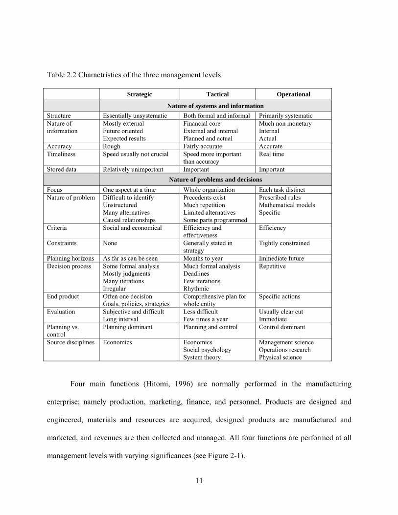
Table 2.2 Charactristics of the three management levels ............................................................. 11
Table 2.3 Simulations of manufacturing systems ........................................................................ 76
Table 2.4 Conceptual differences between DES and SD ............................................................. 92
Table 3.1 Synchronization approaches in distributed simulation .............................................. 112
Table 5.1 Different cases of processing resumption between consecutive DES run segments . 182
Table 5.2 ICOMs for the A-0 IDEF0 model of the SDDES controller ..................................... 195
Table 6.1 Classifying PMOC’s business units in the SDDES model as SD or DES models .... 211
Table 6.2 Abbreviations of module titles and variables ............................................................ 231
Table 6.3 Inputs and outputs of the MIO ................................................................................... 235
Table 6.4 Inputs and outputs of the PWS .................................................................................. 238
Table 6.5 Inputs and outputs of the SD LAB module................................................................ 242
Table 6.6 Inputs and outputs for the PREF module ................................................................... 244
Table 6.7 Inputs and outputs for the PRES module ................................................................... 246
Table 6.8 Testing the difference between the preforms mean production rates – system data vs.
SDDES model data ............................................................................................................. 250
Table 6.9 Testing the difference between presses mean production rates – system data vs.
SDDES model data ............................................................................................................. 251
xxi
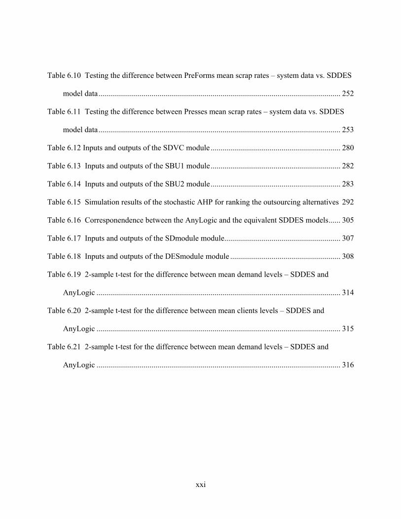
Table 6.10 Testing the difference between PreForms mean scrap rates – system data vs. SDDES
model data ........................................................................................................................... 252
Table 6.11 Testing the difference between Presses mean scrap rates – system data vs. SDDES
model data ........................................................................................................................... 253
Table 6.12 Inputs and outputs of the SDVC module .................................................................. 280
Table 6.13 Inputs and outputs of the SBU1 module .................................................................. 282
Table 6.14 Inputs and outputs of the SBU2 module .................................................................. 283
Table 6.15 Simulation results of the stochastic AHP for ranking the outsourcing alternatives 292
Table 6.16 Corresponendence between the AnyLogic and the equivalent SDDES models ...... 305
Table 6.17 Inputs and outputs of the SDmodule module........................................................... 307
Table 6.18 Inputs and outputs of the DESmodule module ........................................................ 308
Table 6.19 2-sample t-test for the difference between mean demand levels – SDDES and
AnyLogic ............................................................................................................................ 314
Table 6.20 2-sample t-test for the difference between mean clients levels – SDDES and
AnyLogic ............................................................................................................................ 315
Table 6.21 2-sample t-test for the difference between mean demand levels – SDDES and
AnyLogic ............................................................................................................................ 316

1
CHAPTER 1: INTRODUCTION
Businesses are facing unprecedented levels and types of competition at a worldwide
scale. And this environment is continuously evolving. The flat world is pushing higher the levels
of complexity in managing the already complex enterprise systems. The even-more complex
system is the manufacturing enterprise where manufacturing and non-manufacturing functions
coexist. The manufacturing enterprise system is invariably complex dynamic system and this
complexity keeps increasing with the increasing levels of integration and the adoptions of the
system perspectives and those sophisticated information technologies of today. Managers
running such integrated enterprises in such business environments need new dynamic,
comprehensive policy design and testing tools that are effectively and efficiently holistic, yet
simple, scalable, and upgradable as the enterprise evolves.
Dynamism is critical in effectively managing complex systems. Still, managers fail to
account for control actions which have been initiated by them or by others and not yet have their
effects observable because of the misperception of feedback information and time delays
involved in causing the dynamic behaviors of the systems (Lertpatarapong, 2002; Sterman, 2000;
1989). The success of an organization can only be achieved with managing manufacturing and
other functions in a logical association with one another. Policies of empowering and enabling
individuals often prove to be counterproductive unless managers account for the interconnections
and long term impacts of their local decisions (Wu, 2002, Senge and Sterman, 1994).

2
A comprehensive simulation tool that captures the dynamics of the enterprise system and
recognizes the role of feedback information in particular, and in the same time is scalable and
can keep being simple as the enterprise evolves should be of a significant value. In the context of
the manufacturing enterprise, it has moved from being an economy of scale to an economy of
scope and is becoming a global economy of mass customization (Vernadat, 2002). And although
there could be different ways to describe the goal of a manufacturing enterprise, the core of these
is to create money and increase the wealth of the shareholders. All activities within the enterprise
must be streamlined in that direction. Managers need to overcome the traditional organizational
barriers and run their facilities in a more flexible, integrated and dynamic manner.
But trade-offs among various business units’ objectives exist. The fact is that the
manufacturing enterprises consist of manufacturing and non-manufacturing functions. For
instance, the contradictory relationship and the, seemingly, conflict of interests between
accountants and manufacturing analysts have been indicated (Viswanadham, 2000; Reid &
Koljonen, 1999; Sterman et al., 1997; Wu, 1992; Baudin, 1990). Accountants want to limit
spending while manufacturing analysts want more to spend. Many published reports have clearly
indicated the need to combine the aggregate and operational levels of management in simulating
the system. Reported cases showed that using the most advanced equipment and producing the
same product quality as competitors do not offer a competitive advantage (Wu, 1992) unless
marketing, customer relations, financial aspects and other professional supporting functions are
coordinated. Implementing a total quality management (TQM) program can dramatically
improve the operational level performance but could lead to a significant decline in financial

3
performance (Sterman et al., 1997) unless coordination with an overall simulation model of the
organization is achieved.
It becomes impractical to achieve the organization goals unless processes and activities
within the organization are synchronized, coordinated, and integrated. The evolution of the
information systems from materials requirements planning (MRP) via manufacturing resource
planning (MRP II) through computer-integrated manufacturing (CIM) and enterprise resource
planning (ERP) systems reflects this fact.
With the adoption of integration and system approaches in managing the manufacturing
system and the pressure imposed by the increased competition and rapidly changing business
environment, the need has arisen for new simulation modeling tools.
Simulation modeling has been successful and effective in simulating the manufacturing
system. It is traditionally carried out using discrete event simulation (DES). But DES has limited
the scope of simulation to detailed analysis techniques and at the operational levels (Huang et al.,
2003; Smith, 2003; Lee et al., 2002a; Baines and Harrison, 1999). As systems get bigger and
more integrated, DES faces serious challenges. In the one hand the detailed approach of DES is
not appropriate for the strategic aggregate levels of decision making. Besides, the data needed for
such data-driven simulation approach is not normally available at these levels. On the other hand
the complexity of the DES simulation model increases exponentially with the size of system
being modeled. When the focus is the entire manufacturing enterprise system, developing DES
models can be impractical.
The stability of the enterprise system implies the robustness of the system to sources of
variations (equipment failure, performance variation, product changes, sales variations,
4
competitors’ actions, market changes, etc.). Detailed approaches like DES at the operational
levels do not address the problem of stability as well (Rabelo et al., 2005). The complex,
nonlinear cause-and-effect relationships with the impact of the feedback loops and time delays
cause the system to respond to variations in input data with a tendency to amplify them and with
fluctuations. Such fluctuations must be recognized and dealt with through the underlying causes,
not the apparent consequences. The interest in the study of the stability of the system has started
with the application of the control theory concepts to industrial systems by Forrester in the mid
1950s (Edghill and Towill, 1989). The study of stability and reactions to exogenous inputs must
be done before any detailed analyses, and should be done over a long range. Meanwhile, the
assumptions of statistical distributions in the DES cannot be considered fixed over long periods
of time.
Meanwhile, simulations based on system dynamics (SD) methodology (Forrester, 1965)
have showed very good results when used for the simulation of various social and economical
systems. By definition SD is a system thinking approach that follows an integrative perspective
in modeling systems while recognizing the information feedback characteristics so as to show
how organizational structure (in policies), and time delays (in decisions and actions) interact to
influence the behavior of the system (Forrester, 1965).
SD is appropriate as a system thinking approach, for modeling large systems and the
higher levels of decision making where aggregation is preferred. An SD model is an intuitive
dynamic picture of the perceived cause-and-effect relationships among the real system
components. It focuses on system structure and the policy decisions that are embodied in the
feedback loops, not on individual localized decisions or hypothesized data. Much less data is

5
required for SD than for DES. The complexity of the model increases linearly so that complex
system can be modeled with relatively simple models.
SD offers a theory of behavior of systems and it emphasizes the understanding of how
behavior results from corporate structure and policies. It targets top management levels and is
intrinsically appropriate for the design of management policies. Some of its application areas are
corporate planning and policy design, supply chain management, public management and policy,
biological and medical modeling, energy and environment, theory development in natural and
social sciences, complex nonlinear dynamics and others.
We propose to combine the SD and DES in a hybrid discrete-continuous approach (we
will call it SDDES) to simulate the manufacturing enterprise. This simulation methodology is
expected to offer a simple, comprehensive, scalable, non-expensive dynamic policy design tool
that fits the different scopes and planning frequencies of management levels. It combines the
effectiveness of DES at the operational and detailed levels with the simplicity and overall system
thinking approach of SD at the aggregate levels of management. The SDDES enterprise
simulation model is proposed to consist of a comprehensive SD model for the enterprise system
and connected to it is a number of DES models for selected operational and tactical functions as
dictated by the analysis needs.
Because of the differences in structure, view of the world, state updating method, and
time advance mechanisms, of the SD and DES simulations, the combination of them will follow
a distributed-simulation-like arrangement that will be implemented in a modular format. There
are no special requirements that SD or DES simulations have to meet to be utilized in SDDES.
This implies the need for a methodology to synchronize these simulations. A synchronization

6
algorithm is proposed for that purpose along with the communication controller whose function
is managing the interacting simulations and implementing the synchronization algorithm.
1.1 The Purpose of This Research
This research recognizes the difficulties and challenges facing the use of DES techniques
in simulating the integrated manufacturing enterprise, and the potentials and opportunities that
SD offers as a continuous, system thinking approach to develop comprehensive simulation
models of large scale complex systems. This research also investigates the adequacy of the
existing hybrid and distributed simulation approaches in satisfying the needs of simulating the
integrated manufacturing enterprise system. The research proposes and develops a hybrid
continuous-discrete simulation methodology that combines SD and DES to simulate the
manufacturing enterprise. The new methodology is directed towards building simulation models
that are sophisticated yet simple and inexpensive and can encompass the aggregate and
operational decision making levels in the enterprise to support management in developing their
policies and testing them comprehensively.
1.2 Research Premises and Directions
This research follows and investigates the following research directions:

7
1. Managers of the integrated manufacturing systems need new simulation tools that can
accommodate the differences between management levels in a holistic, enterprise-
wide level.
2. Simulation models of modern manufacturing systems should incorporate in the same
simulation, the operational and the aggregate management levels in a dynamic
feedback-based structure
3. Current discrete and continuous simulation approaches fall short in meeting the
challenges created by integration in manufacturing enterprises
4. The simulation of the integrated manufacturing enterprise should be approached using
new hybrid continuous-discrete methodologies
5. The existing frameworks to implement hybrid simulation are inadequate for meeting
the needs of managing an integrated manufacturing enterprise
6. SD and DES can complement each other for simulating the large, dynamic, integrated
manufacturing enterprise system
1.3 Contributions
The contributions of this research include the following:
1. A new hybrid system dynamics-discrete event simulation approach that has the potential
to overcome the difficulties facing existing simulation techniques for the simulation of
the manufacturing enterprise system. The new approach allows using existing/legacy
simulation models and does not require learning new simulation skills.

8
2. A new synchronization mechanism to coordinate the interactions between the continuous
system dynamic models and the discrete event simulation models.
3. A functional design of the SDDES controller that is the core of the SDDES simulation
approach. It implements the synchronization mechanism and manages the interactions
between the SD and DES models.
4. An approach to extend the applicability of SD to the manufacturing applications and
overcome its limitations in modeling detailed situation.
5. An approach to enhance the usability of DES in modeling large complex systems and
overcoming the challenges it is currently facing
1.4 Chapter Outline
The remaining of this dissertation is organized as follows. Chapter 2 presents a review of
the literature related to the research objectives. And as the proposed SDDES uses a distributed
simulation-like structure, Chapter 3 studies the existing synchronization methodologies for the
distributed simulation arrangements. Chapter 4 describes the research methodology. Chapter 5
describes the design of the SDDES simulation framework: the modular structure, the SDDES
module formalism, the synchronization mechanism, and the communication controller. Chapter 6
presents the results of the experimental analysis of the proposed methodology. Chapter 7
summarizes the conclusions of the work and suggest directions for further research.
9
CHAPTER 2: LITERATURE REVIEW
This chapter reviews and discusses the concepts related to this research, starting with an
introduction to the manufacturing enterprise as viewed in this work. A brief review of the
enterprise resource planning systems as they are often used to refer to the enterprise system itself
will be made. Then a review of the enterprise modeling and simulation approaches will be
presented with more details about the discrete and continuous simulation. The application of the
different paradigms of simulation to the manufacturing system domain will then be discussed
leading to defining the perceived gap in simulating the modern manufacturing system with the
existing simulation modeling techniques.
2.1 The Manufacturing Enterprise System
The decision making processes in business systems are classified into strategic, tactical,
and operational levels. Examples of activities performed and decisions made at each
management level are shown in Table 2-1. The strategic level activities include establishing the
philosophy and goals of the enterprise, formulating the management policies, allocating
resources, and determining new products and investments. The tactical level activities are based
on the strategic decisions and include establishing the functional control objectives, planning and
selecting courses of action, acquiring and allocating resources to divisions and departments,

10
preparing detailed work programs, and determining improvement plans. The operational level
activities are the execution of the tactical decisions. They include measuring performance and
preparing performance reports, in particular, about the exceptional or unusual performances. A
comparison with respect to the nature of systems and information and types of problems and
decisions is presented in Table 2-2 (Anthony and Jovindarajan, 1998; Hitomi, 1996).
Table 2.1 Example of contents of activities at the management levels
Strategic Level Tactical Level Operational Level Choosing company objectives Formulating budgets Planning the organization Planning staff level Controlling hiring Setting personnel policies Formulating personnel practices Implementing policies Setting financial policies Working capital planning Controlling credit extensions Setting marketing policies Formulating advertising programs Placement of advertising Setting research policies Controlling research organization Choosing new product lines Choosing product improvements Acquiring a new division Deciding on plant rearrangements Scheduling production Deciding on non routine capital expenditures
Deciding on routine capital expenditures
Acquiring unrelated business New product or product brand line Order entry Adding product line Expanding a plant Production scheduling Adding direct-mail selling Advertising budget Booking TV commercials Changing debt/equity ratio Issuing new dept Cash management Inventory speculation policy Deciding inventory levels Reordering an item Formulating decision rules for
operational control Controlling inventory
Measuring, appraising, and improving management performance
Measuring, appraising, and improving workers’ efficiency
The classification of an activity or a decision as strategic, tactical, or operational should
not ignore the overlaps between the strategic and tactical and between the tactical and
operational. Such overlaps should occur in coordinated integrative way. Dealing with a function
as strategic, tactical or operational should be based on the scope of the impact of the decisions
made in that function.
11
Table 2.2 Charactristics of the three management levels
Strategic Tactical Operational
Nature of systems and information Structure Essentially unsystematic Both formal and informal Primarily systematic Nature of information
Mostly external Future oriented Expected results
Financial core External and internal Planned and actual
Much non monetary Internal Actual
Accuracy Rough Fairly accurate Accurate Timeliness Speed usually not crucial Speed more important
than accuracy Real time
Stored data Relatively unimportant Important Important Nature of problems and decisions Focus One aspect at a time Whole organization Each task distinct Nature of problem Difficult to identify
Unstructured Many alternatives Causal relationships
Precedents exist Much repetition Limited alternatives Some parts programmed
Prescribed rules Mathematical models Specific
Criteria Social and economical Efficiency and effectiveness
Efficiency
Constraints None Generally stated in strategy
Tightly constrained
Planning horizons As far as can be seen Months to year Immediate future Decision process Some formal analysis
Mostly judgments Many iterations Irregular
Much formal analysis Deadlines Few iterations Rhythmic
Repetitive
End product Often one decision Goals, policies, strategies
Comprehensive plan for whole entity
Specific actions
Evaluation Subjective and difficult Long interval
Less difficult Few times a year
Usually clear cut Immediate
Planning vs. control
Planning dominant Planning and control Control dominant
Source disciplines Economics Economics Social psychology System theory
Management science Operations research Physical science
Four main functions (Hitomi, 1996) are normally performed in the manufacturing
enterprise; namely production, marketing, finance, and personnel. Products are designed and
engineered, materials and resources are acquired, designed products are manufactured and
marketed, and revenues are then collected and managed. All four functions are performed at all
management levels with varying significances (see Figure 2-1).

12
Figure 2.1 Functional structure levels in the manufacturing enterprise
The classification into different management levels, and the differences between
functions and tasks performed at each level imply that these differences must be considered in
analyzing the performance of the enterprise. Data in the operational control is in real time and
relates to individual events, whereas data at the aggregate management levels is either
prospective or retrospective and summarizes many separate events over relatively long intervals
of time. Operational control uses exact data whereas higher management levels can use
approximations.
It was noted (Anthony, 1998) that a system that can display to the management the
current status of every individual activity could be developed but it should not be, because
aggregate levels only need to know that the process is, or is not proceeding as planned; without
too much details. Researchers have recognized these differences in the needed levels of details in
data at the different management levels (Lee et al., 2002b; Zulch et al., 2002; Shapiro, 2001;
Baines and Harrison, 1999). This becomes more important in the large-sized, integrated
enterprise systems of today.

13
In our view, it is not only the differences in the levels of details in data that should be
recognized. The frequency of needing data, revisions, and making decisions should also be
considered. A view of the interactions between the management levels should consider an
aggregation/disaggregation (data and time wise) function as depicted by Figure 2-2, where a
triangle below line represents aggregation and a triangle above line represents disaggregation.
Figure 2.2 Interactions among the three management levels
The distinction and the need to recognize the differences between the management levels
becomes even more significant in the manufacturing enterprise due to the unique characteristic
of the manufacturing enterprise which is the presence of the manufacturing functions and
14
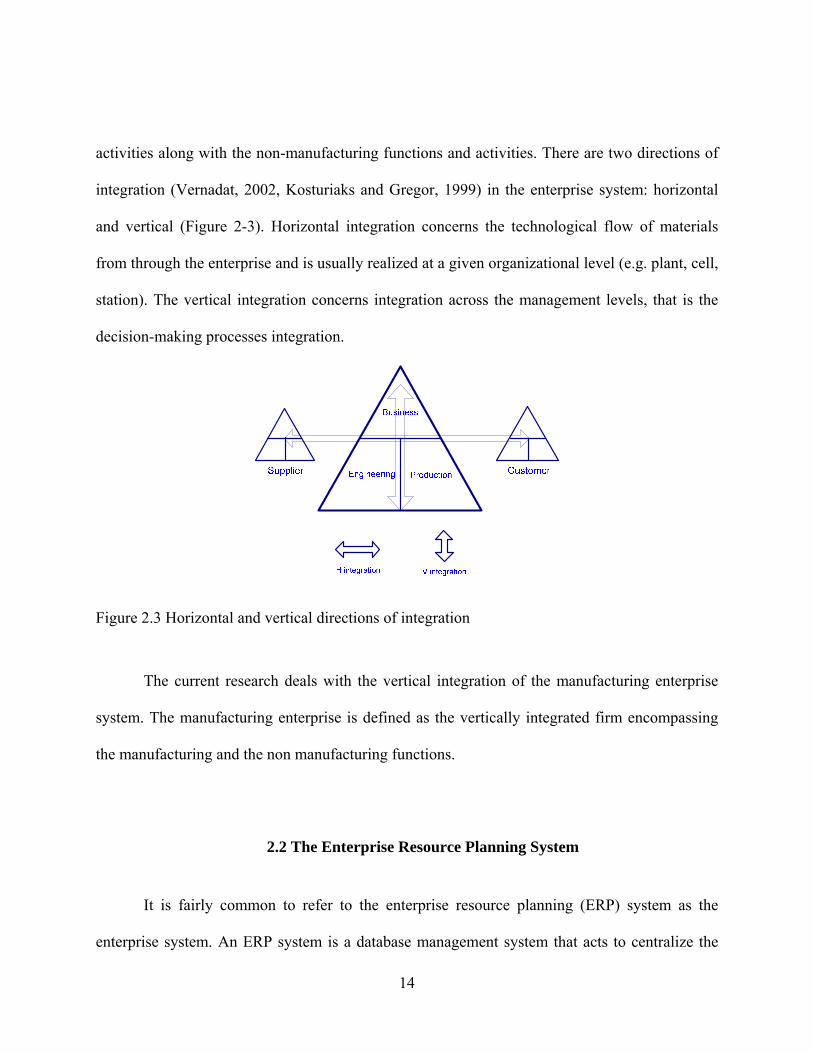
activities along with the non-manufacturing functions and activities. There are two directions of
integration (Vernadat, 2002, Kosturiaks and Gregor, 1999) in the enterprise system: horizontal
and vertical (Figure 2-3). Horizontal integration concerns the technological flow of materials
from through the enterprise and is usually realized at a given organizational level (e.g. plant, cell,
station). The vertical integration concerns integration across the management levels, that is the
decision-making processes integration.
Figure 2.3 Horizontal and vertical directions of integration
The current research deals with the vertical integration of the manufacturing enterprise
system. The manufacturing enterprise is defined as the vertically integrated firm encompassing
the manufacturing and the non manufacturing functions.
2.2 The Enterprise Resource Planning System
It is fairly common to refer to the enterprise resource planning (ERP) system as the
enterprise system. An ERP system is a database management system that acts to centralize the

15
enterprise transactional data and distribute it to users. ERP is the third generation of data
management systems. The first generation; the materials requirements planning (MRP) was
developed in the 1970s in production scheduling contexts, to optimize materials inventories. The
manufacturing resource planning system (MRP II), about a decade later extended MRP to
become more comprehensive. It is a computer-based planning and scheduling and data
management system designed for support the management's control over the manufacturing
activities (Moustakis, 2000). First ERP systems were developed in the 1990s to run MRP II in a
more integrated structure across all business units of the enterprise.
ERP is meant to ensure that every transaction in every activity within the enterprise is
recorded. The risk associated with implementing ERP is huge (Botta-Genoulaz et al., 2005,
Davenport, 2000). Implementation success rates in western companies, including big
corporations, are around 33% according to Botta-Genoulaz et al. (2005) who also stated that:
“… it is not enough to acquire the most advanced information systems to achieve better performance and integration. It is how usable these systems are … ERP systems should be extended by decision-making tools. This is one significant factor toward realizing the promise of ERP … But there are yet more serious issues”.
Among these issues, assuming a successful ERP implementation is the appropriation of
the system by its user, which is often seriously difficult (Hermosillo Worley et al., 2005). A
common side effect is the use of the electronic spreadsheets despite the presence of an active
ERP system. Further, it is necessary for implementing ERP that the enterprise conducts a
business process reengineering and remodeling for ERP to take over the enterprise data and
information. By this it imposes a hierarchy on the company that reduces the flexibility and may

16
create a rigid system, which can make future evolutions of the enterprise hard (Dillard and
Yuthas, 2006).
The development of MRP, MRP II, and ERP indicates the increasing size of the of the
enterprise system and the increasing levels of integration and needs for better management of the
system. Modeling approaches can be advantageous over such transactional data management
systems in establishing better coordination and understanding of the behavior and performance
of the enterprise. Modeling can add the ability to perform what-if analysis and capture the
inherent dynamics of the system to create future projections of behavior.
2.3 Enterprise Modeling and Integration
The current work is motivated by the integration in business systems. Enterprise
integration concepts emerged, like other paradigms, as a result of the advances in information
technologies and the changes in the business environment. Enterprise modeling (EM) is a
prerequisite for enterprise integration (EI). A model is a description of a system or a situation
that can be used to understand its behavior. EM is a representation of the structure, activities,
processes, information flows, resources, people, behavior, goals, and constraints of a business. It
can be both descriptive and definitional (Vernadat, 2002; Barton et al., 2001; Fox and Gruninger,
1998). The role of an enterprise model is to develop enterprise design, analysis, and operational
perspective. EI on the other hand implies breaking down the organizational barriers between the
system units to improve synergy so that business goals are achieved in a more productive and
efficient way.

17
The enterprise modeling and integration (EMI) techniques are particularly concerned
with the creation of models to support the design of integrated systems. The capabilities of these
are unlikely to match the requirements at the operational decision making in manufacturing
systems (Barton et al., 2001). The existing approaches for EM tend to offer fundamentally static
models while providing little support for modeling the dynamics of the systems. Further, the
enabling technologies to reuse and re-integrate EM models as the enterprise system evolves are
lacking (Chatha and Weston, 2005). Meanwhile the manufacturing systems and other business
systems, once designed and started, are inherently dynamic complex systems that evolve and
change their behaviors over time.
2.4 Simulation Modeling
Systems can be modeled by physical or logical models. Logical models are also called
mathematical models and they are either analytical or simulation models. The analytical models
are many types including linear and integer programming, network models, and other operations
research tools. The use of such models requires many assumptions and simplifications, which
cannot always be practical. Relaxing these assumptions would make models very complex and
unwieldy for analysis.
Simulation is a form of modeling that is used to dynamically analyze and evaluate the
performance of systems as it changes over time to make future inferences. Technically,
simulation is the process of designing and creating a computerized model of a real or proposed
system for the purpose of conducting numerical experiments, for better understanding of its

18
behavior for a given set of conditions. Simulation is more flexible than the mathematical
analytical models and does not generally require those assumptions made with the analytical
models. Virtually, any system can be simulated at any level of details.
Simulation models can be deterministic or stochastic. Deterministic models describe the
system’s dynamic behavior assuming no random effects and give same output for the same input.
Stochastic simulation models describe the dynamic behavior when there are random effects and
they give only estimates of the true system response since outputs are random variables
themselves. This necessitates the need for several runs of the models to estimate the system
response with the minimum variance.
Simulation models can also be discrete or continuous depending on how the variables
included in the model change over time. When the state of the system (represented by selected
variables) changes discretely at specified points in simulated time then the simulation model is
discrete and those points in time are the event times. When the change is continuous over
simulated time and is cause by the progress of time then the model is continuous (Banks et al.,
2005; Pritsker et al., 1997).
There are two ways of being discrete: the time-stepped and the event-stepped (Law and
Kelton, 2000). Time-stepped models update the system state at each preset time step. Event-
stepped (event-driven) models update the system state upon the occurrence of some events that
affects the state. Event-driven (discrete event simulation; DES) is the common discrete
simulation approach.
Figure 2-4 compares continuous and discrete system state updating. The state is updated
only at times of the occurrence of the events (the start or the end of an activity). Between events

19
the state is ignored or assumed unchanged. In continuous simulation the state variables are
defined as functions of time and they change in value because of time passing. Simulation time
in DES advances from an event time to an event time. In continuous simulation, time advances in
fixed steps. The step size is selected to achieve the desirable accuracy.
Figure 2.4 Updating state over simulated time in continuous and discrete simulation
Ignoring the system state between events in DES can lead to erroneous evaluation of the
system performance. The validity of this assumption depends on the nature of the system being
modeled and the desirable accuracy and resolution of the simulation model. For instance, assume
a machining workstation that is modeled by a DES model. If the system state is measured by the
number of parts at the workstation, then the state does not change except by the events of the
arrival and departure of the parts. If the state variable of interest is the level of completeness of
processing then it has to be observed continuously because as long as the workstation is running
values of the level of completeness is changing. Observing the machine at the events of start or
finish may not be enough to describe its behavior.

20
The point being made here is that there are parameters and situations in the same system
that are better be simulated by DES and others that better be simulated by continuous simulation.
In practice, DES is commonly used to approximate continuous parameters. If, for instance, a
continuous variable is approximated by DES, due to the way the state is updated in DES
overestimation or underestimation of the continuous parameter will be obtained. This is depicted
in Figure 2-5. Further, there may not be events to be assumed in an efficient way to reduce the
times between events in order to improve the approximation.
Sta
te
Figure 2.5 Discrete vs. continuous state estimates
2.4.1 Discrete event simulation
The entity-flow view is the common DES simulation approach. Entities flow through the
system and compete for the resources and use these resources to do activities or have activities
done onto them. If resources are busy, entities wait in queues until resources become available.
Seizing a resource, releasing it, starting or ending an activity, and entering or exiting the system,

21
etc. are all events. Events are timeless occurrences and only their occurrence can change the
system state. The terms in italics above are the core elements of the DES model.
The simulation calendar is a list of events that are scheduled to occur during the
simulation time. Upon the occurrence of an event the simulation engine schedules new events
and/or reschedule others. For example, an entity seizes a resource. The simulation engine
samples the time needed for the entity to end sizing the resource (seizure duration, e.g.
processing time) and schedules the resource-release event and adds it to the calendar at a time
equal to current time plus the resource seizure duration. Each entry in the calendar is made of the
entity identifier, activity that the entity will interact with, and the event time. There are three
ways to describe and define a DES model, as noted by Pritsker et al. (1997). These are by
describing the changes in the state at each event time, describing the activities in which the
entities engage, or describing the processes thorough which the entities flow. Consequently the
DES model can be viewed in three ways:
1. The event view in which the modeler determines the events that change the state of
the system and develops the logic of their occurrence. The model is the
implementation of that logic.
2. The activity scanning view in which the modeler determines the activities that the
entities engage and the conditions that cause the start or the end of the activities. This
implies specifying the events in an indirect way. Events start and end the activities.
Here the events are not explicitly scheduled. Instead they are linked to activities-
related conditions that when true the events are scheduled and executed. The

22
conditions are scanned during the simulation time and all included activities must be
scanned for their conditions at each time step.
3. The process interaction view which takes a relatively comprehensive approach to
define the flow of entities through the system.
2.4.1.1 Output analysis in DES
DES is driven using data that are generated using appropriate probability distributions.
Durations of activities, number of expected events, arrival rate, etc are all sampled using
probability distributions that are chosen for fitting the real data in the real system at the best
feasible level of accuracy. Consequently, model outputs are random variables and must be
interpreted using statistical techniques.
The analysis of simulation output should consider whether the system is terminating or
non-terminating. A terminating system has specific starting and ending conditions, which define
the simulation run length. Run replications are necessary. Replications are repetitions of the
model run using different sets of random numbers. This creates independent, identically
distributed samples of data that can be analyzed statistically.
Analyzing the output of a DES model is summarized herein based on Law and Kelton
(2000). Assume a terminating DES model that is run for n replications. Let X be the state
variable of interest. For replication nj ,...,2,1= , the random variable jX represents the state
variable value for the replication. Unbiased point estimators for the mean and variance of the
state variable are given by equations (1) and (2).

23
∑=
=n
i
i
nXnX
1
)( (1)
1
))(()( 1
2
2
−
−=∑=
n
nXXnS
n
ii
(2)
A )%1(100 α− confidence interval for the mean is calculated using equation (3), where
)2/(1,1 α−−nt is the α-quartile of the t-distribution with 1−n degrees of freedom.
nnStnX n
)()(2
2/1,1 α−−± (3)
The correctness of the confidence interval given by (3) depends on the assumption that
the sX j ' are normal random variables. This assumption is rarely satisfied in practice and more
stochastic investigations must be performed to assess the robustness of the confidence interval
before making inferences on the performance of the system.
A non-terminating system on the other hand has no defined end conditions. A
manufacturing system can be modeled as a non-terminating system where, although there may be
shifts and workers may arrive and leave at specified times, the system itself is running
continuously and each day is a continuation of the previous day. To analyze a non-terminating
system a very long simulation run is made of the steady state performance is analyzed. The
single long run is divided into sequences of observations that are approximately independent of
each other. The batches of observations are used as if they are replications of a terminating
system. The batch size is a function in the correlation structure of the system response. Batch
size should be at least 10 times as large as the largest lag for which the correlation between
observations remains significant. However, correlation will still be there. Observations at the end

24
of a batch are correlated to observations at the beginning of the following batch. But if the batch
length is large enough compared to the time extent of the correlation between individual
observations then the approximation is acceptable. Pegden et al. (1990) recommended between
10 and 20 batches.
The elimination of the initial bias from the output is the hardest problem in analyzing the
non-terminating simulations. Let X be the steady state random variable for a state variable in the
simulation model and n data points nXXX ,...,, 21 are collected for estimating its mean. Assume
I as the initial system state (initial condition). As ∞→n , )Pr()/Pr( xXIxXn ≤→≤ . The
steady-state mean of X is given by equation (4).
( )IXE nn|lim
∞→=μ (4)
This makes estimating the mean hard as a finite n cannot be sufficient unless I is
eliminated. A common way to do so is the graphical way of Welch (1983) which uses k
independent runs each producing n observations, then an across-runs averages are computed by
formula (5) (Alexopoulos and Kim, 2002):
njXk
Xk
iijj ,...,11
1
== ∑=
(5)
Moving averages are then plotted for a given time window w against j . If a smooth plot
results then observations up to j are truncated. If not smooth another time window is used. The
choice of the time window can be a difficult problem. In addition, the truncated observations
waste the computing resources before they are excluded.

25
DES has been an effective approach to simulate complex system and manufacturing
systems in particular (at the manufacturing functions side as shown later in this chapter). It can
describe the most complex systems, at any level of details. It allows analysts to track the status of
individual entities and resources and to estimate numerous performance measures. However, it
suffers major drawbacks. Analysts can only establish estimates of and correlations among
variables and performance measures using statistics. Understanding the differences between
correlation and causality is not always easy, especially when modeling the contemporary large
sized integrated manufacturing systems. As was briefly shown the statistical analysis of the
simulation output, being terminating or non-terminating can be a tedious task that becomes
harder as the system becomes bigger and complex. Further, at the strategic levels, these outputs
are hard to comprehend.
DES models allow analysts to evaluate the system performance for specific values of
decision variables or control policies. They do not allow for determining the stability of the
system in any region or neighborhood of those values or policies. This is critically important in
complex systems where performance may be driven by hidden causal relationships that could be
highly non-linear. In such systems, small deviations from the optimal decision point can cause
disproportionately large changes in the system performance.
In addition to that, DES is too demanding for data. The task of input data preparation can
be very difficult and tedious. Building and validating models is a very time and resources
consuming. And the complexity of the model increases exponentially as the size of the system
being modeled increases.

26
In a manufacturing enterprise, detailed data at the operational level are normally available
at detailed levels. At aggregate management levels, data is not normally available in the level of
details needed by DES (Zulch et al. 2002; Anthony and Govindarajan 1998). The qualitative and
continuous nature of aggregate management levels parameters, also, creates challenges to the use
of DES at these levels (Zulch et al. 2002; Baines and Harrison 1999). These drawbacks with
DES become more critical when attempting to simulate the integrated manufacturing system. A
review of reported cases is presented in a later section.
2.4.2 Continuous simulation
In continuous simulations the state variables change continuously over time. Such models
often require the construction of influence diagrams (cause-and-effect diagrams) that show the
relationships and interactions among the set of system variables. Associated with the influence
diagrams is a set of mathematical equations that describe the rate of change of the state variables
with respect to time. This set of equation is solved to estimate the system state. Compared to
DES this is an important advantage since DES has no standardized way for describing the
systems (Wu, 1992). Continuous simulations are generally more intuitive, simpler to build, and
they need much less data and data preparation than DES. The state of the system in continuous
models is known for any point in time not only at certain points in time.
A continuous system can be represented by the vector of its state variables; ℜ∈X
(Formula 6) where the set of n state variables; niXi ,...,2,1, = changes in values continuously
with time t :

27
[ ]TnXXX L21=X (6)
In practice, the state equation is not known. Instead the rates of change of the state
variables over time are defined (Pritsker et al., 1997). Consequently, derivatives (the rate of
change equations) are used in continuous simulation models. Only first order differential
equations are used. If higher order equations are involved, they can be converted into first order
sets. Differential equations are called ordinary if all of its derivatives relate to the same variable;
typically time in simulation applications (Wu, 1992; Pegden et al., 1990).
Conceptually, a continuous simulation model is used to find solutions to complex
differential equations using numerical techniques and given a set of initial conditions. Analytical
solutions of these differential equations are practically impossible. Randomness may or may not
be introduced but most often, continuous simulations are deterministic.
2.4.2.1 System Dynamics simulation
System dynamics (SD) (Forrester, 1965) is a well-elaborated methodology for continuous
simulation. It is useful in capturing the dynamics of complex real world systems where delays
and feedback loops are in effect. The fundamental concept is the recognition of the complex,
nonlinear feedback processes inherent in the structure of the system. Economic and industrial
activities are closed loop, information feedback systems, and models of such systems should
preserve the closed loop structure. SD is the application of feedback concepts to social systems
for analyzing and designing robust policies rather than making optimal decisions based on

28
assumed forecasts. SD is a system thinking approach that takes an integrative perspective in
modeling systems. Forester saw it as an approach to solving important problems at the top
management levels (Sterman, 2000; Lyneis, 1980; Forrester, 1975; 1965).
SD uses causal and feedback loop structure and a few diagramming tools to describe the
relationships among the factors that affect the performance of a dynamic system. The main
diagramming tools are the stocks (also called levels) that are usually used to represent the system
state variables, and the flows (also called rates) that represent the factors or the actions (the
policies of the management) that influence the stocks. Stocks are modeled mathematically as the
time integration of the sum of the flows connected to them. Flows can be modeled by any
relevant form of mathematical relationships. Computer simulation is then used to solve these
equations such that deterministic simulation experiments are conducted.
Feedback loops can be negative or positive based on the direction of influence that
parameters have on each other. A negative loop is a series of causal relationships that tend to
force behavior towards a certain goal value. A positive loop is self-reinforcing; it amplifies
disturbances in the system to create even higher variations in behavior. Figure 2-6 shows a
negative and a positive causal relationships and a positive feedback loop.

29
Figure 2.6 Negative and positive causal relationships and feedback loop in SD
The overlapping feedback loops that make up the model structure are mapped into stocks
and flow rates. Stocks are mapped into time integrations. They accumulate the results of taken
actions in the system. They create system continuity between points in time and they are changed
only by flows. The flows depend only on present values of the stocks and other constant input
values. They are mapped into simple algebraic formulas.
Stocks and flows are represented by rectangles and valves respectively. In Figure 2-7,
Inventory and Goods on Orders are two stocks. Each stock can have one or more flows flowing
into or out of it to increase or decrease its value. The arrows represent causal relationships. For
instance Order Rate is a flow that is a function in Desired Order Rate, Adjustment time, Desired
inventory level, and Inventory. Parameters other than stocks or flows are the auxiliary variables.
The formulas for flows can be long and complex. To simplify them, they are broken down into
pieces each represented by an auxiliary variable. Then the flow's formula is made up of these
variables. The negative sign beneath Goods on Order indicates a negative feedback loop that
Market Share Demand Deliveries Inventories+ -
Link polarity is positive. IfMarket share increases then
Demand increases
Link polarity is negative. IfDeliveries increase then
Inventory decrease
Market share.
Demand.Ordres filled
Production
+
+
+
+

30
starts with Order Rate, passes through Goods on Order, Arrival Rate, and Inventory, and ends at
Order Rate.
Figure 2.7 Levels and rates symbols as used in SD models
The SD model in its final form is the set of stocks that are interconnected by the set of
flow rates, in an alternating fashion, as symbolized in Figure 2-8, in which stocks are rectangles
and flows are valves. The arrows denote the relationships between them. The dashed arrows
denote sharing data.
Figure 2.8 Generic structure of the SD model (Forrester, 1965)
Desired orderrate
Goods onOrderOrder Rate
InventoryArrival Rate Usage Rate
Adjustmenttime
Desied inventorylevel
Arrival delay Demand

31
The structure of Figure 2-8 implies that the stocks are influenced only through the flows
while the flows are dependent on the stocks; that is dependent on the state of the system. For
instance, in a manufacturing system, stocks can be the levels of the accounts payable or
receivable, or the levels of inventories. The flows are the policies of managing inventory,
production rate that uses the inventory, the policy of collecting or paying the accounts. Only
through the policies the stock level can be changed. And for the management to decide the
appropriate policies it has to monitor the stocks. The presence of feedback loops can be observed
since stocks determine flows and flows influence stocks. A SD model in fact is a collection of
overlapping feedback loops the capture the mutual interactions among all system components.
Building a model starts with the identification of the related parameters to the objective of
analysis then defining the causal relationships among them in a feedback structure. The stocks
and flows are then defined out of these parameters and the model is finally mapped into the
mathematical formulation.
When mapped into mathematical formulas, this structure should be able to describe any
cause and effect relationship in the system while being mathematically simple. And as indicated
by Forrester (1965, 1975) it should handle continuous interactions such that any discontinuities
introduced by solution-time intervals (because of using numerical methods) do not affect the
results. It should however be able to generate discontinuous changes in decisions when these are
needed (which makes it the proper choice of a continuous approach for SDDES, where it
interacts with independent DES models)
Solving a SD model starts with initializing the values of the stocks; that is the initial state
of the system must be known. Given the state of the system, the management determines its

32
policy to run and influence the system evolution and performance over time. Having determined
the policy and set the system parameters by the management considering the starting system
state, the new values of the stocks (new system state) can be calculated by adding the impacts of
the policy (flow rates) on the starting state values. Flow rates (management actions) work to
increase or decrease the values of the stocks. New system state then allows the management to
review and modify, if needed, the policies undertaken. This loop continues until the end of the
planning horizon. The rule is that stocks (system state) can only be influenced through the flow
rates. This is realistic. For instance, the management cannot increase its product inventory except
by increasing the production rate.
The continuous advance of time is broken into very infinitesimal time intervals of
magnitude tΔ . Numerical techniques are used. Figure 2-9 shows the calculations sequence in SD
(Forrester, 1965). If current time is 2t then the state (stocks) should be known at 1t . The system
advances from 1t to 2t to reach system state at 2t . The state at 2t is the result of the state at 1t
plus the effect of the flow rates during tΔ from 1t to 2t . At 2t , the stocks are calculated and
using them the flow rates for tΔ from 2t to 3t are calculated. And once they are calculated then
the system state at 3t can be determined. This calculations sequence reduces the dependence of
the state on the old states. Only the state before tΔ is used.
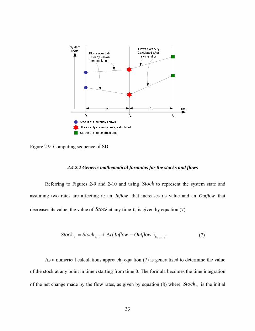
33
Figure 2.9 Computing sequence of SD
2.4.2.2 Generic mathematical formulas for the stocks and flows
Referring to Figures 2-9 and 2-10 and using Stock to represent the system state and
assuming two rates are affecting it: an Inflow that increases its value and an Outflow that
decreases its value, the value of Stock at any time it is given by equation (7):
)(1 1)(
−−− −Δ+=iiii tttt OutflowInflowtStockStock (7)
As a numerical calculations approach, equation (7) is generalized to determine the value
of the stock at any point in time tstarting from time 0. The formula becomes the time integration
of the net change made by the flow rates, as given by equation (8) where 0Stock is the initial

34
value of Stock. This is equivalent to the SD model structure shown in Figure 2-10 (without the
Delay variable or the curved arrows).
∫ −+=t
t dtOutFlowInflowStockStock0
0 )( (8)
Figure 2.10 Stock and flow represented in SD models
On the other hand flows can take many mathematical forms. Still they are functions in the
stocks. Flows are calculated for every time interval tΔ . The value of the flow rate is the slope of
the curve that represents the behavior of the stock over tΔ . Flows are functions in the values of
the stocks they are related to at the beginning of the interval. If a stock is to contain entities of
any type (units of products, people, cash, water, etc.) then flows are then measured in terms of
entities per unit time. From Figure 2-10, the Outflow is defined by equation (9). The Inflow can
be a function of other stocks in the models, not necessarily the one shown in the figure.
Delay
StockOutflow i
ii
ttt
1
1)(−
−=− (9)
The parameter Delay in equation (8) is a time period defined in the context of the system
being modeled. It is the average time needed for the entire population of Stock to flow to the
StockInflow Outflow
DelayStock0

35
next part of the system at the Outflow rate. Outflow rate is the rate at which the population of the
Stock leaves, so the rate is the size of the population divided by the time needed for the
population to leave completely.
The formulas for flows are usually broken down into smaller components should they be
complicated. In this case auxiliary variables are added to the SD model and each of them is
calculated based on management policies as functions in the system state. Then auxiliary
variables are algebraically summed to make up the definition of the flow. This maintains the fact
that flows are functions in the stocks. Using auxiliaries simplifies model development and allows
modelers to record information about detailed issues in the system structure. Consequently,
auxiliaries and flows are functions in stocks and other auxiliaries. Equation (10) is generic for
flows and for auxiliaries, where f and g are arbitrary functions.
),(),(
sAuxiliarieStocksgsAuxiliariesAuxiliarieStocksfFlows
==
(10)
Delays are critical in SD models. The presence of time delays creates the dynamics in the
system. Sterman (2000) emphasized that the inability of managers to recognize the impact of
delays in the feedback system contributes to all problems faced by them. A stock is not normally
consumed up or filled instantaneously. It takes time to build up inventory, for instance, and to
deplete it. A management policy to order raw material at a certain rate will take time before
making observable effect on the inventory level (until materials arrives from the supplier). This

36
delay between actions and their impacts is the source of dynamics in the system and must be
recognized in the model, which is the case in SD.
Equation (9) is a simple situation where it takes the time period Delay to consume the
level of Stock. This is called first order delay function and it results in a simple exponential
behavior of Stock over time. If the flow is a function in two cascaded stocks then a second order
delay is present in the system. A stock-flow structure that creates 3rd order delays can be as
shown in Figure 2-11. This is common in modeling manufacturing processes. Equation (9)
applies here such that the outflow of the first level is the inflow to the next, and so on. Degrees
higher than three can be defined similarly.
Figure 2.11 Third order delay structure in SD
The behaviors due to the 1st, 2nd, and 3rd order delays are shown in Figure 2-12 assuming
a step increase in the input to the system. According to the real behavior of the system being
modeled, the choice of the degree of delay in the definition of flows is made.
Stock 1 Stock 2 Stock 3Flow 1 to 2 Flow 2 to 3 OutflowInflow
Delay/3 Delay/3. .Delay/3

37
Figure 2.12 Behaviors of SD stocks due to various delays (Sterman, 2000)
The above description of the SD model shows a relatively simple approach that gives it
an advantage over DES in modeling larger systems. Besides the minimal needs of data makes SD
more appropriate than DES at the aggregate management levels. Further, SD by definition
targets top management levels (Forrester, 1965) offering a strategic systemic view.
Industrial and economic systems are closed-loop feedback information systems. SD
particularly recognizes the role of feedback information in creating system behavior. It offers a
quantitative approach for relating organizational structure and corporate policy to growth and
stability. Besides, such a closed-loop system exhibits behavior as a whole that is not evident
from the examination of the individual parts and components of the system (Sterman, 2000).
Major executive decisions represent a continuous process. Decisions are reached after a period of
consideration. Actions are not taken immediately after decisions. Decisions are interpreted and
smoothed and they then produce gradual changes as they overcome the resistance and inertia of
the business units in the organization.
In any industrial system, there are usually considerable levels of aggregation. For
example orders arrive as separate pieces of paper, but they are represented as a continuous order
flow. The executives’ interest, anyway, is above the level of individual transactions. A

38
continuous flow model helps to concentrate attention on the central framework of the system
structure, which is more orderly and unchanged than what would be thought. Diversion of
attention toward separate isolated events tends to obscure the central structure of the system that
we are trying to define and maintain running. A model should represent the continuously
interacting forces in the system. The frequency with which measurements on real systems may
happen to have been taken is not relevant to the frequency with which internal dynamic
performance must be calculated (Sterman, 2000; Lyneis, 1980; Forrester, 1965).
Certain modeling requirements of the manufacturing system that SD can support are
listed below:
1. A number of subsystems can be integrated to give a holistic system view. Manufacturing
systems are made up of several units for which SD can offer an umbrella for integrative
interactions.
2. It is appropriate as a system thinking approach, for modeling large scale systems and the
higher levels of decision making where aggregation is preferred.
3. It focuses on the policy decisions that are embodied in the feedback loops, not on
individual localized decisions.
4. It focuses on system structures not on hypothesized data and much less data is required
than in DES
5. Strategic issues can be analyzed over long time horizons without difficulties with the
statistical assumptions
6. Stability of the system can be analyzed for long time horizons even with minimum data.

39
7. It is easily generalized and generic concepts already exist for the different types of
systems.
8. A model is an intuitive dynamic picture of the perceived cause-and-effect relationship
among the real system components that is easy to present to top management personnel.
9. The complexity of the models increases linearly (Sterman, 2000) so that more complex
systems can be modeled with relatively simple models.
2.4.2.3 The stock management model
It was predicted by Forrester (1991) that about 20 generic SD models would be
developed to represent 90% of situations encountered by managers in enterprises. In fact, the
majority of the SD models reviewed for this research uses some of Forrester’s concepts he
included in his early models in the 1950s. Forrester built models for a simple supply chain
(Forrester, 1965; 1968) and for the whole world's economical dynamics (Forrester, 1973) using
the same few modeling tools of SD. Sterman (1989) developed the stock management model
(SMM) as a generic structure for modeling business functions. He combined Forrester’s concepts
as well as the works of Lyneis (1980) and Morecroft (1985). Sterman used SMM in building a
comprehensive organization model in Sterman et al. (1997) and in his book Business Dynamics
(Sterman, 2000). Lynies (1980) also explained a number of generic model concepts that were
closely similar to Stermn’s.
The SMM is a generic structure of the decision making problem concerned with the
regulation of a system state. Decision makers facing such a problem seek to maintain the stock
level at a particular target value. But stocks cannot be controlled directly and have to be

40
influenced through the flow rates. The decision maker adjusts these flows such that the stock is
at its desirable level. What makes the problem difficult is the presence of time delays between
the initiation of a control action and the effect of that action. Further, there are time lags between
changes occurring in a stock’s level and the perception of these changes.
SMM is divided into two sections: the stock and flow structure, which represents the
physical structure of the real system, and the decision making rules by which managers act to
maintain the physical flow in equilibrium. The basic physical flow structure is made up of two
stocks and three flows (Figure 2-13). It can represent the ordering of materials in a production
system and receiving them, the work-in-process level and the finished products level, the level of
people being hired and the level of workforce, or the accounts receivable and the money in hand
and many other cases. Order Rate is the rate of ordering materials from suppliers. Supply on
Order is the materials that have been ordered but not yet arrived. Acquisition Rate is the rate at
which the materials that have been ordered arrive. Stock is the accumulated materials that have
arrived. Loss Rate is the rate at which the materials are taken from the inventory. It has to be
dependent on the value of the Stock. Similarly the Acquisition Rate has to be dependent on the
Supply on Order level. Order Rate is a function of any meaningful parameters in the system.
The Acquisition Delay and Loss Rate both include some external parameters in their
definitions. Loss rate can be influenced by customer order rate, attrition rate of people, recovery
rate of patients, etc. Management can try to influence its value. Similarly Acquisition delay can
be influenced by the management by arrangements with suppliers or some worker agents for
example.

41
Figure 2.13 The stock management model structure
The management should set the policies to regulate the two state variables. There are
desired levels for them that are decided by the management. As a control task, management
monitors the actual levels and compares them with the desired levels to estimate the adjustments
needed to maintain the target values. An adjustment however is over a period of time, not
instantly. Some time is needed to move from the actual to the desired level. The action that the
management actually takes to accomplish the adjustment is making new orders. So the
adjustment policy will lead to estimating the Indicated Order Rate, which what the management
believes the order rate that must be in effect to accomplish the adjustments, i.e. to maintain the
system states at target values.
Supply On Order StockOrder Rate Acquisition Rate Loss Rate
Acquisition Delay+
-
++
External Factors
Internal Factors
Adjustment forStock level
Adjustment forSupply On Order
level
Desired Stock
Time toadjust Stock
Desired SupplyOn Order
Time to adjustSupply On Order
Expected Loss Rate
IndicatedOrders
Stock &Flow
Structure
DecisionMaking
Rule
.
. 0

42
The Indicated Order Rate is the outcome of the policy setting process. Yet some input
from other, mostly external parameters are needed. In the current example, it is the Loss Rate,
i.e. the customer order rate or usage rate. The management should also estimate the expected loss
rate so that its adjustment policy does not result in accumulating unnecessary stocks. This
technically closes the feedback loop in which the adjustment policy is embodied. This feedback
loop starts at the Loss Rate and ends at the Loss Rate. More examples of using the SMM are
presented in Sterman (2000).
2.5 Hybrid Simulation
The world does not usually lend itself to using one form of abstraction at a time. Most, if
not all real life systems; physical, industrial, business, social, environmental etc. are hybrid in
nature. Whenever human decisions impact the system behavior and the environment, the hybrid
systems can be better approximations (Lee et al., 2004; Lee et at., 2002b; Borshchev, et al.,
2000; Zeigler et al., 2000). Using hybrid techniques is becoming a must as has been said by some
(Levin and Liven, 2003). Modern technology applications; cars, robot, cell phones, digital
watches, medical devices microwaves, washing machines, etc. are all areas for applying hybrid
systems. By hybrid simulations we mean combined discrete-continuous simulations, which gives
modelers the ability to reach better fidelity and fit the characteristics of all sections of the system
being modeled. Approximating continuous behavior by discrete behavior cannot guarantee
accuracy. Overestimates or underestimates will likely be obtained. An experiment made by Lee

43
et al. (2002a) to compare modeling the inventory level in a supply chain system by DES and by
continuous simulation showed that the DES model overestimated the level of inventory.
The previous two sections in this chapter highlighted the inherent complexity in
developing discrete models and the simplicity in developing continuous models. The modeling
of large, complex systems can be made easier if hybrid simulation of the two approaches is used.
In addition this can accommodate all types of behavior in the system which, for being realistic,
cannot be only discrete or only continuous. Two directions of interactions (Ziegler, 2000;
Pritsker et al., 1997) can occur between discrete and continuous components in a hybrid
simulation as shown in Figure 2-14.
Figure 2.14 Types of interactions between continuous and discrete components
Hybrid simulation models combine discrete and continuous behaviors, or as expressed by
Maler et al. (1992) have non-trivial mixture of discrete and continuous components. Research
related to this field has been more popular in the area of real-time control and reactive systems.
Reactive systems are event-driven systems that are normally interacting with external and
internal stimuli. They maintain ongoing interaction with the environment rather than giving
results upon termination. These systems are generally discrete in nature but have to interact with
environments that are continuous. Definitions used by researchers have been conceptually the

44
same. Most researchers who are interested in hybrid systems came from the areas of control
systems and the theoretical computer science and they viewed the hybrid system as the system
that combines the discrete and continuous state changes; usually in distributed and embedded
control systems (Gheorghe et al., 2006; Lee et al., 2004; Lee and Hsu, 2002; Alur et al., 2000;
Chouikha, et al., 2000; Pepyne et al., 2000; Kowalewski et al., 1999; Maler et al., 1992; Harel
1987). Common examples of hybrid systems in literatures are systems such as the digital
controller of a continuous environment, air traffic management systems, guidance of
transportation systems, embedded automotive controllers, real-time communication networks,
control of process and manufacturing plants, chemical processes, robot planning, and the like.
Researchers also have used hybrid approaches for business systems, including supply
chains and some manufacturing applications. In most cases, decision making situations were
simulated using discrete simulation with few differential equations for some continuous variables
under the control of the discrete parts of the simulation model (Umeda and Zhang, 2008; Lee et
al., 2004; Gregoriades and Karakostas, 2003; GroBler et al., 2003; Levin and Levin, 2003, 2002;
Lee et al., 2002a; Zulch et al., 2002; Pepyne et al., 2000; Baines and Harrison, 1999; and others).
Hybrid systems research in the area of simulation modeling of the business, environment,
manufacturing systems started from the recognitions of the limitations of the discrete event
simulation approaches. This was particularly significant as the business, supply chains, and
manufacturing systems have become more integrated, complex, and larger in size. Still, this
review shows that even when the system control is not the focus in the simulation, hybrid
simulation are based on the discrete controller of the continuous system elements. The next

45
section describes the two main approaches to describe the dynamics of the hybrid continuous
discrete simulations.
2.5.1 The dynamics of hybrid systems
There are two main approaches to develop hybrid simulations:
1. The hybrid state transition machine (Maler et al., 1992; Harel, 1987).
2. The DEVS&DESS formalism (Ziegler et al., 2000; Ziegler, 1976)
Fundamental similarities between the two approaches can be observed:
1. Both were developed based on a control-system mentality; that is a digital (discrete)
system controlling a continuous environment.
2. Running a hybrid simulation is a process of alternating between a discrete phase and a
continuous phase. In the discrete phase the state of the system changes and time does
not advance. In the continuous phase the time advances but the system state does not
change.
3. Events drive the simulation model and only events update the system state.
4. Continuous calculations are performed in the continuous phase between the discrete
events, starting with the new state after the event occurrence.
5. The impact of the continuous calculation is communicated to the discrete components
by a discrete event, which is triggered by the continuous variable value crossing a
predefined threshold level

46
6. Both require the use of small-sized objects for which the states can be easily
enumerated as well as transitions between states.
2.5.2 The hybrid state transition machine
The state machine/diagram is one of the Unified Modeling Language (UML) tools
(Jacobson et al., 2001). Called the state chart diagram in UML, it addresses the dynamic view of
the system by showing the sequence of states that an object goes through during its lifetime in
response to events, together with its responses to those events. Most of the characteristics of the
state machine as used currently in simulation modeling were described by Harel (1987). Maler et
al. (1992) modified Harel’ state machine to incorporate the continuous behavior.
The state diagram is a directed graph in which nodes represent states and arrows (labeled
with triggering events and guarding conditions) represent transitions between states (Figure 2-
15). It works by following this rule: If event a occurs while the system is in state A and if
condition P is true at that time, then the system transfers to state C. The symbol )(Pa indicates
that the event a cannot cause the transition to be taken unless condition P is true. Condition P is
a guarding condition in the sense that it prevents the transition if it would lead to a wrong or
illogical state. For example, a machine cannot switch from idle to busy unless power is on.
Events can be associated with conditions (e.g. event a ) or be unconditioned (e.g. event x ). If
unconditioned the transition is taken once the event occurs.

47
Figure 2.15 State diagram with three states
The state diagram as described above is a discrete event driven system. Maler et al.
(1992) incorporated the continuous behavior into the discrete state diagram by using the concept
of phase transition, by which the behavior of a system is the result of alternating discrete and
continuous phases. The continuous phase takes positive time to allow changes in variables that
are modeled by differential equations. The discrete phase consists of a finite number of discrete
transitions that may cause abrupt change in the value of the variables. To incorporate the
continuous behavior into the discrete system, the state (on a state diagram) is allowed to have
differential/integral equations associated with it to describe the continuous behavior when the
system is in that state. The behaviors of the variables modeled by the differential/integral
equations (continuously behaving variables) are sensed at the state diagram transitions and based
on the values of these variables they can generate events that would lead to transitions to be
taken or at least enabled.
Because of the need to alternate between the continuous and discrete phases, a hybrid
system can either advance time (the continuous phase) or update the state (the discrete phase).
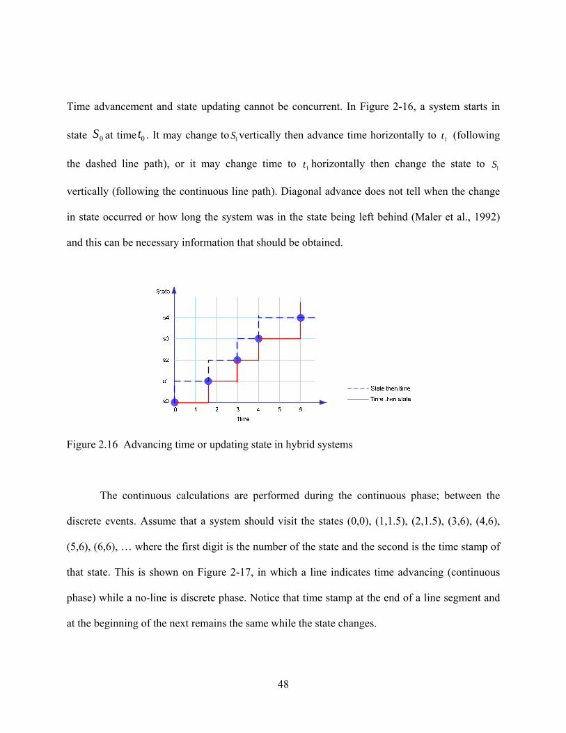
48
Time advancement and state updating cannot be concurrent. In Figure 2-16, a system starts in
state 0S at time 0t . It may change to 1S vertically then advance time horizontally to 1t (following
the dashed line path), or it may change time to 1t horizontally then change the state to 1S
vertically (following the continuous line path). Diagonal advance does not tell when the change
in state occurred or how long the system was in the state being left behind (Maler et al., 1992)
and this can be necessary information that should be obtained.
Figure 2.16 Advancing time or updating state in hybrid systems
The continuous calculations are performed during the continuous phase; between the
discrete events. Assume that a system should visit the states (0,0), (1,1.5), (2,1.5), (3,6), (4,6),
(5,6), (6,6), … where the first digit is the number of the state and the second is the time stamp of
that state. This is shown on Figure 2-17, in which a line indicates time advancing (continuous
phase) while a no-line is discrete phase. Notice that time stamp at the end of a line segment and
at the beginning of the next remains the same while the state changes.
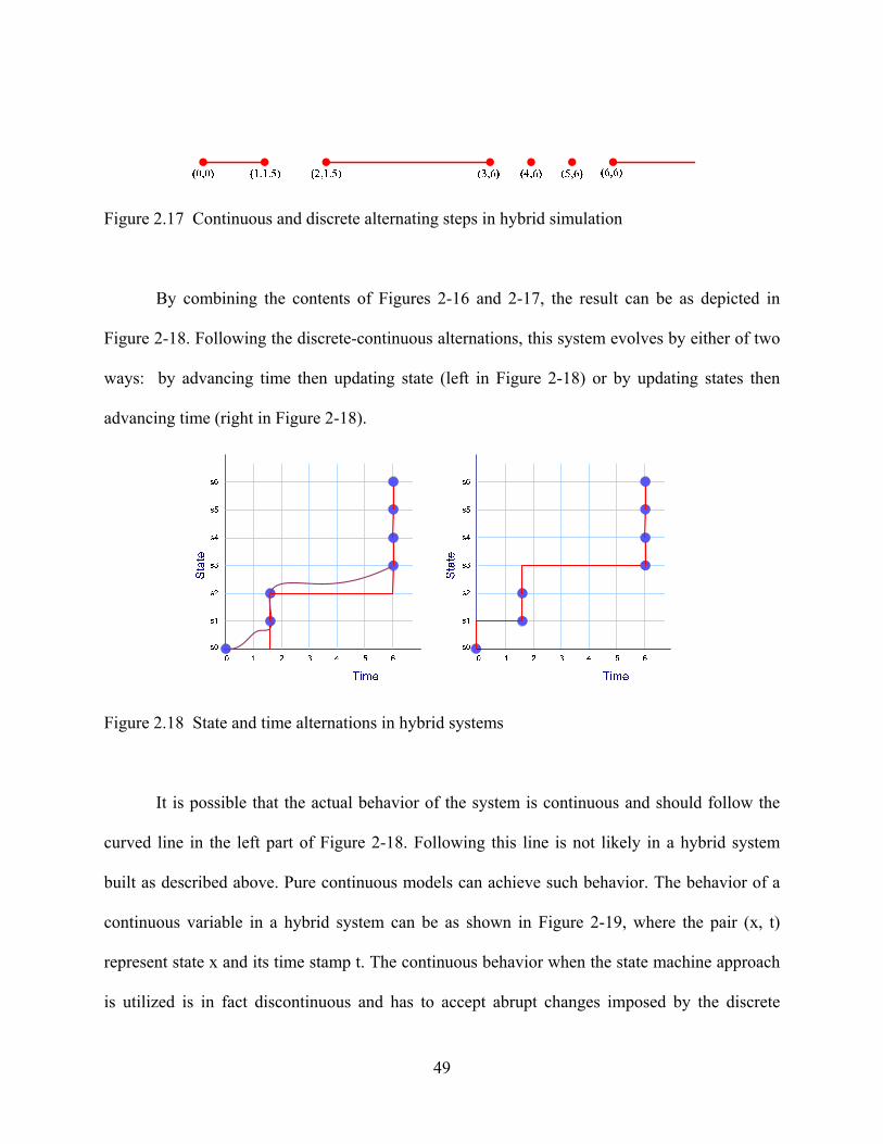
49
Figure 2.17 Continuous and discrete alternating steps in hybrid simulation
By combining the contents of Figures 2-16 and 2-17, the result can be as depicted in
Figure 2-18. Following the discrete-continuous alternations, this system evolves by either of two
ways: by advancing time then updating state (left in Figure 2-18) or by updating states then
advancing time (right in Figure 2-18).
Figure 2.18 State and time alternations in hybrid systems
It is possible that the actual behavior of the system is continuous and should follow the
curved line in the left part of Figure 2-18. Following this line is not likely in a hybrid system
built as described above. Pure continuous models can achieve such behavior. The behavior of a
continuous variable in a hybrid system can be as shown in Figure 2-19, where the pair (x, t)
represent state x and its time stamp t. The continuous behavior when the state machine approach
is utilized is in fact discontinuous and has to accept abrupt changes imposed by the discrete

50
components. Discrete always dominates the simulation in this approach. In Figure 2-19, the State
Event is a discrete event generated by the continuous variable crossing a predefined threshold
value. This event is communicated to the discrete components and is then treated as any regular
discrete event. This is how a continuous variable may attempt to change the system.
Figure 2.19 Intermittent continuous behavior in control-based hybrid simulation
2.5.2.1 The AnyLogic software package
The commercial software AnyLogic (http://www.xjtek.com/) is marketed as the only
commercial software that combines DES and SD modeling tools in the same interface. It offers
tools to build discrete simulation and system dynamics models as well as agent-based models in
an object oriented environment. AnyLogic is an implementation of the concepts proposed by
Harel (1987) and Maler et al. (1992) in the way it combines the discrete and continuous
simulation units. AnyLogic uses an object oriented approach with state charts associated with the

51
objects in the model. The state chart indicates the state space of the object and the events or
conditions that cause it to take transitions from a state to another. It can also describe actions that
result from state change. For instance, a state chart of an object from an AnyLogic model is
shown in Figure 2-20, where a system is initially using the main generator. The transition from
main generator to a standby generator (the left most arrow) is taken if a message arrives at the
object that the main generator is down. The transition from using the standby generator to B
(branch) can be timed or based on an event. If a message that the main generator has been fixed
arrives before the end of the time interval then the transition will be to using the main generator
state, otherwise the transition will be to the stop state to stop the system at the end of the time
interval.
Figure 2.20 State chart in an AnyLogic object
A message arriving to take a transition is an event. Alternatively the transition can be set
to react directly to the occurrence of events by writing a Java code that instructs the transition
how to react. Events are all discrete and timeless. Thus AnyLogic allows discrete and continuous
model objects to interact through the use of the state chart. The value of a continuous variable
can be monitored to trigger an event that is sensed at a transition as defined in the Java code in it.
Main Generator
Standby Generator
StopB

52
A special type of events (the dynamic event) is an object in AnyLogic that is used as a simple
form of the state chart and can be used in the same way to react to events or act based on
specified points in time. The dynamic event object allows the modeler to explicitly schedule a
discrete event based on a condition associated with the value of some model variable that might
be a continuous variable, or based on time. When the condition is true, the event is triggered and
the system state is updated as dictated by the action defined in the event object.
Another way to interact continuous and discrete model parts depend on the fact that the
continuous components in AnyLogic are treated as variables not objects. The DES components
are objects. Since they are variable, the stocks and flows of a SD model can be referenced in the
actions coded in the DES objects as well as in the state chart and the dynamic event code fields.
It is also possible to reference the attributes of the DES objects in the mathematical formulations
of the SD variables. For instance the size attribute of a DES queue object, which is modeling
materials buffer between two processes, can be referenced in the definition of the work-in-
process level in a SD model unit. This however can be misleading since the SD concepts do not
allow stocks to be changed except by the effect of the flow rates. The contents of a DES queue
should be added to a SD stock only through a flow rate variable. AnyLogic allows the simple
algebraic addition of the queue contents to SD stock.
The users of AnyLogic need to be Java programmers. All actions or reactions in any
object are stated as Java statements. Sophisticated object behaviors can only be defined in this
way. The AnyLogic simulation engine is discrete but uses a numerical solver to solve the set of
differential equations of the SD variables. Figure 2-21 represents the simulation engine
architecture of AnyLogic. The discrete engine generates a set of global algebraic differential
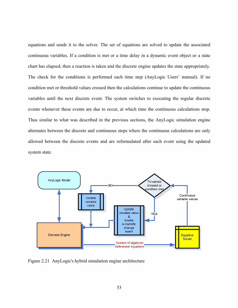
53
equations and sends it to the solver. The set of equations are solved to update the associated
continuous variables. If a condition is met or a time delay in a dynamic event object or a state
chart has elapsed, then a reaction is taken and the discrete engine updates the state appropriately.
The check for the conditions is performed each time step (AnyLogic Users’ manual). If no
condition met or threshold values crossed then the calculations continue to update the continuous
variables until the next discrete event. The system switches to executing the regular discrete
events whenever these events are due to occur, at which time the continuous calculations stop.
Thus similar to what was described in the previous sections, the AnyLogic simulation engine
alternates between the discrete and continuous steps where the continuous calculations are only
allowed between the discrete events and are reformulated after each event using the updated
system state.
Figure 2.21 AnyLogic's hybrid simulation engine architecture

54
Based on AnyLogic’s user manual, Figure 2-22 describes the alternating between the
discrete and continuous steps. In the continuous step time advances to the nearest event (or
events) in the events queue while solving the algebraic-differential equations (part (a)). At the
next event’s time the event is executed, the state of the system is updated, time does not advance,
and the events queue may be changed by deleting and/or scheduling events (part (b)). The
following continuous step (part (c)) is the same as in part (a) but an event (Q: called change
event) defined by the use of the dynamic event object or the state chart occurs unexpectedly. The
continuous event is stopped to execute Q (part (d). The following continuous step is same as that
in (a) or (c). The sequence continues in the way to the end of the simulation run.
The discrete part of AnyLogic engine does not know when a change event would occur.
It depends on the equations set being solved to read the time for that event. Once this happens,
the clock is advanced to the time reported by the continuous-time equation solver, and the event
is executed by the discrete part. Continuous behavior affects the discrete behavior in this way.
On the other hand, each time an event is executed, the system state changes and the updated state
is used in the continuous part as new initial conditions for the calculations and the simulation
engine generates a new set of equations to replace the existing set. In this way the discrete part is
impacting the continuous time behavior. This mechanism is comparable to Figures 16 through 19
in the previous sections.

55
Figure 2.22 Continuous and discrete steps in AnyLogic

56
2.5.2.2 Commentary on using the state chart and AnyLogic
AnyLogic is the implementation of the hybrid state chart technology. This technology
was originally developed for reactive and real-time control systems. Objects are preferred to use
state charts and AnyLogic uses objects. In business and social systems the use of the state chart
can be tedious as there is a need to enumerate all states that a system can be in during its life
time. The number of the states can be infinite in general business and social systems. In physical
and control system these states can be enumerated whereas in social system this task can be
impractical, unless some accuracy or oversimplifying assumptions are considered. Lee at al.
(2004) have recognized this difficulty even for the model of a digital controller of a single
printed circuit board production process. Allowing one type of behavior to control the other is
the disadvantage of the state chart. As mentioned by Frey et al. (1997) a central design issue in
developing hybrid discrete-continuous simulations is which paradigm controls the other. Yet
there is no answer to this question yet.
The continuous behavior of the hybrid state chart is discontinuous as was shown in
Figure 2-19. In social and business systems an abrupt change in the value of a continuous
variable is not realistic. The change in customer order rate, productivity, material arrival rate, the
rate of increase of a population, the level of pollution, or may be the learning curve of a certain
process are not expected to show such abrupt changes. In such situations, continuously changing
variables are not normally influenced by such timeless events. For example, if the inflation rate
in the market is crossing a threshold value, there is no way to just cut it. Government and market
actors have to change their policies to influence the inflation rate over a period of time. Also if
inventory is increasing at a certain rate, management may not empty the inventory suddenly in

57
the normal operating circumstances. It may stop production and the inventory would go down
gradually.
In addition, it is not likely that single simulation software can meet all needs of all
modelers particularly if hybrid simulation is required. In that regard, AnyLogic users need to use
Java to add needed object classes and extend existing ones. In that way, AnyLogic becomes an
interface for a programming language.
An approach that can integrate different discrete and continuous simulation software can
be advantageous as it would allow molders to keep using their expertise in the modeling
approach they prefer. It would also offer the flexibility to use the simulation software that is most
appropriate for the specific needs, then have it integrated to other software that were also chosen
for specific advantages in them. This can also allow modular, scalable models which could
simplify the modeling process. This is what this research work is proposing. One major feature
of the proposed approach, unlike AnyLogic, is the ability to utilize the existing simulations
(legacy simulations) without having to learn a new approach or resort to lengthy programming
work.
2.5.3 The DEVS-based hybrid simulation
The DEV&DESS formalism is an approach to specify and describe the dynamics of the
hybrid continuous discrete systems. It is a combination of the DEVS (Discrete Event System
Specification) and the DESS (Differential Equation System Specification) formalisms. All of
them; DEVS, DESS, and DEV&DESS are the works of Zeigler (1976) and Zeigler et al. (2000).

58
2.5.3.1 The DEVS formalism
DEVS is a general formalism for discrete event system modeling based on set theory. It
describes the different sets in a simulation model and the functions that describe the relations
between these sets. Three sets and four functions are used in the basic DEVS formalism:
1. The set of inputs
2. The set of outputs
3. The set of states
4. The internal transition function
5. The external transition function
6. The output function
7. The time advance function
Any system can have a set of states that it can be in during its lifetime. The system
receives inputs through input ports and gives outputs through output ports. The ports are the
communication channels through which the system interacts with other systems or the
environment. The DEVS representation of the system is given as in equation (10).
(10)
1. X is the set of external inputs (external input events)
2. Y is the set of outputs (output events)
),,,,,,( int taSYXDEVS ext λδδ=

59
3. S is the set of sequential states. S is defined before hand and each state Ss∈ has a
specified time point )(sta at which it expires.
4. extδ is the external state transition function. It represents the interactions between X
and Q to describe how inputs cause state transitions. It creates a state trajectory over
S . It can be defined by SXQext →×:δ where Q is defined below.
5. intδ is the internal state transition function. It describes how transitions between states
in S are taken when their times come; i.e. how to transit from s when )(sta is
reached. It can be described by SS →:intδ
6. λ is the output function. It is defined for the active state only (active state is the state
that has finite duration as opposed to passive states that has infinite time durations).
λ is executed only when the elapsed time for the system in a state equals its life time
duration. Output is generated upon internal state transitions only, just before the
transition is taken. λ creates a trajectory over Y and is given by YS →:λ
7. ta is the time advance function. For a state Ss∈ it represents the time until which the
system remains in that state if no external events occur. It creates a trajectory of states
over the positive time domain: { }∞∪ℜ→ +Sta :
Let Q be the set of total states. An element in Q is the pair of a state and the time elapsed
since the system entered that state. If the elapsed time is represented by e , then Q is defined by
Formula 11.

60
(11)
Unless an external input causes a transition from s the system would internally undergo
a transition when )(stae = . Upon the transition and reaching a new state the elapsed time
counter; e is reset to zero.
2.5.3.2 The DESS formalism
DESS is a version of the DEVS formalism, for the differential equations models
(continuous models) in DESS the state transition function of DEVS is replaced by a rate of
change function that defines the rates of change of the state variables. Numerical techniques are
used to perform the calculations at the preferred time step. Let nqqq ,...,, 21 be the state variables
and mxxx ,...,, 21 be the input variables, then a continuous model is formed by the set of first-order
differential equations of (12):
(12)
{ })(0,|),(: staeSsesQ ≤≤∈
))(),...,(),(),(),...,(),(()(....
))(),...,(),(),(),...,(),(()(
))(),...,(),(),(),...,(),(()(
21211
212121
212111
txtxtxtqtqtqfdt
tdq
txtxtxtqtqtqfdt
tdq
txtxtxtqtqtqfdt
tdq
nnn
nn
nn
=
=
=

61
The DESS formalism specifies the differential equation simulation models with three sets
and two functions (DEVS uses three sets and four functions) and can be represented by equation
(13).
(13)
• { }ℜ∈∈= cccc vInportspvpX ,||),( is the set of input ports and values.
• { }ℜ∈∈= cccc vOutPortspvpY ,|),( is the set of output ports and values.
• Qis the set of states
• QXQf →×: is the rate of change function
• λ is the output function, which can relate Q to Y or relate Q and X to Y. Thus it
has two forms: YQ →:λ and YXQ →×:λ
DESS describes a time-driven approach that cannot easily capture the feedback structure
of the continuous system. States have to be defined, which puts limits on the size of the system
that can be specified.
2.5.3.3 The DEV&DESS formalism
To develop hybrid simulation models, DEVS and DESS are combined (Figure 2-23) to
form the DEV&DESS system specification formalism.
),,,,( λfQYXDESS =

62
Figure 2.23 DEV&DESS combined model (Zeigler et al., 2000)
The DEV&DESS formalism uses five sets and six functions to specify a hybrid model. It
is represented by equation (16).
(16)
• and are sets of discrete event inputs and outputs.
• is the structured set of
continuous inputs with input variables contix . Being a continuous in nature this could
be a list of values that are changing with time. It could be a step function input to a
continuous system, a formula describing a flow rate of increase or decrease defined
over a certain period of time. The period of time may be as small as an integration
step.
),,,,,,,,,,,(& int fCSSYYXXDESSDEV contdiscext
contdisccontdisccontdiscr λλδδ=
discX discY
{ },...,|,...),( 221121contcontcontcontcontcontcont XxXxxxX ∈∈=

63
• is the structured set of continuous
value outputs with output variables . This is again a set of values over time. The
output can be the behavior of the continuous state variable over a period of time, not
just a value at a certain point in time.
• and are sets of discrete and continuous states respectively. To combine
them is the set of states as a Cartesian product of discrete and
continuous states
• is the external state transition function, where is the set
of total states; defined as
• is the internal state transition function
• is the event output function; executes only when an event
occurs.
• is the continuous output function
• is the rate of change function
• is the state event detection condition predicate
The DEV&DESS system behaves following combinations of the following three cases
over its life time, assuming an interval >< 21, tt :
{ },...,|,...),( 221121contcontcontcontcontcontcont YyYyyyY ∈∈=
contiy
discS contS
contdisc SSS ×=
SXXQ disccontext →××:δ Q
{ }+ℜ∈∈= 0,|),( eSsesQ
SXQ cont →×:intδ
disccontdisc YXQ →×:λ
contcontcont YXQ →×:λ
contcont SXSf →×:
BoolXQC cont →×:

64
1. No events during the interval: and specify the continuous behavior. There is no
state transition since there are no events. But new values for the continuous state
variables are calculated. This corresponding to the time phase in the hybrid state chart
approach.
2. A state event at time t during the time interval: A state events implies that
))(),((int txtsC cont is true. A continuous state variable has crossed a threshold value so a
new value is calculated and in addition intδ is executed to define a new state.
3. A discrete event at the external input port at time t during the interval: extδ is
executed to define a new state at t .
The semantics in part 2 above implies that the state event affects the discrete part. In part
3 the time event in the discrete part also affects the continuous part through changing the value
of f . This makes DEV&DESS another form of the same concepts of the hybrid state machine
approach.
2.5.3.4 Commentary on the DEV&DESS formalism
DEV&DESS follows the same approach used in the hybrid state diagram approach. The
DESS part (the continuous) is allowed to cause state events to occur and those events are
detected at the discrete part. This takes place in the same way it does in the hybrid state machine
approach. In the intervals between events, the DESS input, state, and output values change
continuously until a condition specified on the continuous element becomes true. Typically, the
condition is a continuous variable reaching a certain threshold or whenever two continuous
f contλ

65
variables meet (in which case, their difference crosses zero). In such situations, a state event is
generated. This is represented by Figure 2-24 by Ziegler et al. (2000).
Figure 2.24 State event generated at crossing a threshold by continuous variable
The illustrative example that Zeigler et al. (2000) used to illustrate the use of the
DEV&DESS was a barrel filling process. As depicted in Figure 2-25, the discrete input on/off
causes the external transition function to open the valve variable (assuming it was off at start up).
This event changes the rate of change function f at the continuous side, which allows the inflow
to start filling the barrel. The continuous variable Contents represents the level in the barrel. It is
also reflected by the continuous output Cout via the continuous output function. If Contents
reaches the level of 10 the condition is satisfied and a state event is triggered in the discrete side.
This causes the internal transition function to change the state of the discrete (variable Valve) to
off. Also the state event triggers the output function to indicate a barrel finished at the discrete
output barrel.

66
intδextδ discλ
f contλ
Figure 2.25 DEV&DESS hybrid simulation model of a barrel filling process
Such a situation can be modeled as a control process. Temperature in a furnace can
increase until a certain value where discrete action is taken. A robot would move until a distance
is covered then it is stopped. These are examples where the threshold approach is applicable. But
as we argued earlier, it is not realistic to expect all continuous systems to be increasing or
decreasing until crossing a threshold value. In fact the oscillating behavior (Figure 2-26) of
continuous parameters such as inventory or production rate, or capacity, is more expensive and
dangerous in a manufacturing system than a trend in any of them. A threshold cannot be used to
control such a behavior. Management would work to smooth out the oscillation and achieve
stability not to prevent a certain critical value if a critical value could be defined.

67
Figure 2.26 Oscillating continuous behavior not detected by threshold technique
DEV&DESS also requires the definition of states for the continuous components. The
use of objects where each has a specific task to perform would make that possible for only
needing a small set of states and transitions. But this is not likely to be the case for all continuous
systems.
The simulation of a continuous system involves the simultaneous solution of a set of
differential/integral equation. The simultaneous solution implies that the system would be
performing actions for all of variables at the same time. Unlike discrete simulation where events
are handled one at a time, continuous simulation acts concurrently for all elements in it. The
point here is that defining states for continuous behavior is not practical or useful. Control
situations are easy in that regard but not all continuous simulation situations are.
This becomes even more significant with SD. SD follows a system approach to recognize
the impact of the structure of the system and the set of causal relationships in it on its behavior.
Dividing a SD model in small objects and allowing them to interact indirectly would violate the
fundamentals of SD regarding capturing the feedback structure of the system.

68
This implies that in a business system modeled in SD, the definition of states to support
integration to DES models does not offer useful results. The inability to define states makes it
difficult to define a pattern for interactions between a SD model and DES model. The only way
to start defining the interactions between SD and DES is by recognizing when data is needed
from one to the other. These needs for data sharing follow the nature of system being modeled.
In DEVS and state chart approaches, the need to an interaction is signaled by an event. As there
are no events in SD models then the needs to share data should be decided logically based on the
overall function of the system being modeled.
2.5.3.5 Using the DEV&DESS formalism
Few implementations of DEV&DESS could be found in the literature survey in this
work. Ziegler at al. (2000) described a pseudo code for a DEV&DESS simulator that uses
messages between the DEVS and the DESS units to do three tasks: detection of the state events,
reporting the state events, and the execution of the state events. That is events drive the
simulation. Choi et al. (2005) and Choi et al. (2006) modeled the software development process
as a hybrid process but using the DEVS formalism, not DEV&DESS. They connected the DEVS
objects to build a feedback structure and made the simulation advance time in steps rather than
by event occurrences. Their goal was replicating an earlier SD model (Abdel-Hamid and
Madnick, 1991) of the same process. They approximated the continuous behavior by time steps
execution of a DEVS-based model. In their second paper they utilized the condition function of
DESS to detect the state event occurrences. They did not use DEV&DESS; only picked the
condition function to use with a DESS model. In our assessment, the difficulty faced them was

69
the need to define states for the continuous parameters in DEV&DESS. They kept the original
SD model’s logic, which did not allow practical definition of the states for the continuous
parameters when the approximated the process by a DEVS model.
Gheorghe et al. (2006) used the DEVS formalism (the coupled version as described by
Zeigler et al. (2000)) to describe interfacing discrete and continuous models. They approximated
the continuous model by DEVS as well. No use of DESS or DEV&DESS was mentioned. They
only classified the DEVS objects’ ports into ports to receive data from the continuous variables
and ports for receiving data from the discrete components. All units of the system were specified
in DEVS as coupled units. They however proposed a synchronization mechanism to interface
discrete and continuous components, which will be described in Chapter 4. The synchronization
mechanism could detect the discrete or the state events generated in any part of the model, which
is the core task in DEV&DESS simulator of Ziegler et al. (2000). The coupled DEVS version of
DEVS was the framework for their hybrid simulation system, not the DEV&DESS.
2.5.4 On the current hybrid simulation approaches
The discussion of the hybrid state machine and the DEV&DESS approaches to hybrid
simulation as well as the way that AnyLogic works can support the following comments:
1. Both approaches assume a discrete (digital) controller controlling a continuous
environment. The continuous calculations have to be bounded by the discrete events and
be allowed only in segments between events.

70
2. The continuous variable must accept abrupt changes in their values by the occurrence of
the discrete events. A segment of continuous calculations between two events may not be
a natural continuation of the previous segment.
3. DES dominates the hybrid system transforming it into stochastic-like system even if the
deterministic dynamics are of significance. Pepyne and Cassandras (2000) argues that
this shifts the paradigm of analyzing continuous systems from the mature differentiable
calculus to the less mature non-smooth calculus field, which is based on Lipschitz’s
continuity condition.
4. Continuous components do not change the state of the hybrid system except by signaling
the discrete part of reaching a pre-defined threshold value. Discrete events drive the
simulation and only events can update the system state.
5. Defining states for a continuous system, which is controlled by a discrete controller, is
not practical. A continuous variable in fact has an infinite number of states and
identifying them in a simulation model is not practical. Crossing a threshold value is the
only state recognized for continuous variables.
6. The SD methodology offers the ability to understand the system behavior and how it
evolves over time. In the core of the methodology is the use of averaging and smoothing
techniques to identify the trends in the behavior. Using SD in the state chart-based or the
DEVS&DESS-based hybrid systems with the averaging and smoothing will filter out the
exceptional occurrences that may not allow accurate definitions of the thresholds values
that can be used in communication with a discrete system.

71
7. In business and social systems, where continuous behavior is observable, the use of the
state chart can be tedious as there is the need to enumerate all the possible states and the
transitions between them. The same is true for the DEV&DESS formalism as all states
must be stated and transition functions have to be defined.
8. It is not likely that all continuous behavior will be either increasing or decreasing over
time until reaching a threshold value. Fluctuations and oscillatory behavior can be more
expensive and dangerous than a decreasing or an increasing level.
2.6 Distributed Simulation
Distributed simulation implies loosely coupled simulations (Fujimoto, 2000) that interact
intensively at certain points in time. Yet both; parallel and distributed are concerned with issues
introduced by distributing the execution of DES programs over multiple processors and
computing platforms. The technologies of the parallel and distributed simulation were motivated
by the needs of the military applications to integrate the geographically distributed systems
(simulations and others). By the mid 1990s the Distributed Interactive Simulation (DIS) Standard
(IEEE 1278-1995 and the Aggregate Level Simulation Protocol (ALSP) were developed and
used. Currently the High Level Architecture (HLA) has replaced DIS and ALSP as the
framework for developing distributed simulations. Still the military uses are main drivers (Bodoh
and Wieland, 2003; Borshchev et al., 2002; Fujimoto, 2001; 2000).
HLA is a standard (IEEE 1516) that describes the rules that should be followed to
accomplish the integration of disparate simulations. The individual simulations in HLA are

72
called federates while the collection of federates that are incorporated together is called
federations. The software realization of the HLA framework is called the Runtime Infrastructure
(RTI) and it implements the HLA rules and provides methods that can be called and used by
federates. Figure 2-27 is a representation of the HLA structure.
Figure 2.27 Structure of HLA implementation
HLA consists of the three components (Kuhl et al., 2000; Fujimoto, 2000):
1. The HLA rules that federates follow to comply with the HLA standard.
2. The Object Model Template (OMT) that specifies what information is communicated
between federations and how it is documented.
3. Interface specification that defines how HLA members interact with the RTI library. It
defines the RTI services and the application programming interfaces (API) to allow
different programming languages and computing platforms.

73
RTI is responsible for providing support to distributed objects’ interactions, attributes’
ownership, and other optimistic and the time management policies (Bononi et al., 2003).
Specifically, RTI is active in the following areas (Fujimoto, 2000):
1. Federation management, which includes services to create and delete federation
executions, allow federates to join or resign from federations, and pause or resume
executions.
2. Declaration management, which allows simulations to establish the intent to publish
attributes and interactions, and subscribe to be updated about attributes owned by other
simulations.
3. Ownership management, which enables the transfer of ownership of attributes during
executions.
4. Time management, which coordinates the advancement of logical time.
5. Data distribution management, which controls the distribution of state updates among
federations.
2.6.1 Distributed simulation in industry
Distributed simulation usage is very limited in industry (Boer et al., 2006a; Lendermann,
2006). A recent survey on the use of distributed simulation in industry (Boer et al., 2006a;
2006b) has given some explanation where it showed that industry practitioners depend heavily
on the “commercial-off-the-shelf” simulation packages, which offer very limited support for the
HLA standard. Vendors do not see direct benefits in offering HLA support in their packages,

74
given that HLA is still military-directed and too complex for industry applications. Unlike
military applications, industry wants fast and direct result at the lowest expenses, for which HLA
as well as the concepts of distributed simulation would add too high overhead technically and
financially. Vendors also do not see much economical benefits in collaborating with other
vendors. Yet some benefits of distributed simulation have been recognized. These included the
possibility of speeding up the model development process by modularizing models and utilizing
the synchronization techniques.
In manufacturing applications, Saad et al. (2003) suggested that using distributed
simulation for manufacturing system does not require strictly synchronization; only loose level
of synchronization is required in which a model in a distributed arrangement would pause its run
if it detects that it is ahead of other simulations. No more complicated approaches should be
needed according to them. However, this could be true for the specific case they considered
where several models (built by the same tool; Arena) communicated by sending messages using
the Microsoft Windows’ Message Queuing tools. The models represented several processing
operations that communicated with an assembly facility. In the case of simulating the enterprise
in SDDES more considerations must be taken in synchronizing SD and DES models since each
method of simulation works in a different way.
Chapter 4 will review the existing synchronization approaches used in distributed
simulation arrangements. In Chapter 5, we propose a new synchronization mechanism for the
synchronizing SD and DES.

75
2.7 Simulating the Manufacturing Enterprise
DES is the most commonly used approach in modeling the manufacturing system since
the 1960s. Usually the manufacturing activities are simulated. DES as a detailed, stochastic
approach is suitable for simulating manufacturing processes that are highly stochastic and need
to be monitored closely. SD is not widely used in manufacturing applications. But the integrated
manufacturing system is challenging DES and indicating opportunities for exploiting the
potential of SD.
Few surveys have addressed the use of simulation in manufacturing applications. Banks
et al. (2005) and Smith (2003) have surveyed and discussed the applications of DES. Another
limited survey by (Baines and Harrison, 1999) assessed the use of SD in manufacturing systems.
A recent two-part survey (Boer et al., 2006a; 2006b) assessed the use of the distributed
simulation concepts in industry in general. The findings of these surveys are discussed in the
following sections. In addition, cases of applications of simulation in the manufacturing domain
will be discussed. Table 2-3 summarizes representatives of these cases. A discussion follows
after the table.
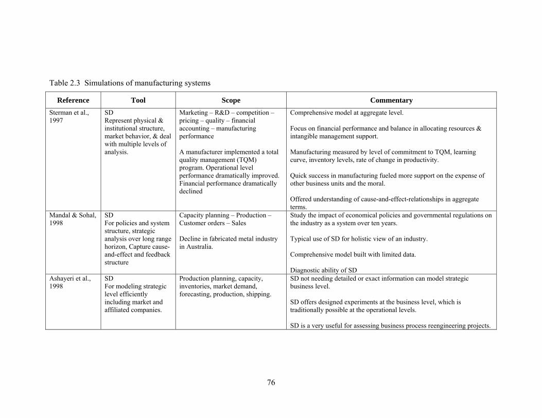
76
Table 2.3 Simulations of manufacturing systems
Reference Tool Scope Commentary Sterman et al., 1997
SD Represent physical & institutional structure, market behavior, & deal with multiple levels of analysis.
Marketing – R&D – competition – pricing – quality – financial accounting – manufacturing performance A manufacturer implemented a total quality management (TQM) program. Operational level performance dramatically improved. Financial performance dramatically declined
Comprehensive model at aggregate level. Focus on financial performance and balance in allocating resources & intangible management support. Manufacturing measured by level of commitment to TQM, learning curve, inventory levels, rate of change in productivity. Quick success in manufacturing fueled more support on the expense of other business units and the moral. Offered understanding of cause-and-effect-relationships in aggregate terms.
Mandal & Sohal, 1998
SD For policies and system structure, strategic analysis over long range horizon, Capture cause-and-effect and feedback structure
Capacity planning – Production – Customer orders – Sales Decline in fabricated metal industry in Australia.
Study the impact of economical policies and governmental regulations on the industry as a system over ten years. Typical use of SD for holistic view of an industry. Comprehensive model built with limited data. Diagnostic ability of SD
Ashayeri et al., 1998
SD For modeling strategic level efficiently including market and affiliated companies.
Production planning, capacity, inventories, market demand, forecasting, production, shipping.
SD not needing detailed or exact information can model strategic business level. SD offers designed experiments at the business level, which is traditionally possible at the operational levels. SD is a very useful for assessing business process reengineering projects.

77
Reference Tool Scope Commentary Fujii et al., 1999
DES Physical materials flow: Processes & transportation Computer Integrated Manufacturing (CIM) system
Distributed simulations arrangement Only physical materials flow in CIM controlled by MRP
Reid & Koljonen, 1999
SD Captures dynamical feedback structure
Abstract representation of lead time, inventory levels, management capacity to deal with problems, Delayed orders Analyzed the theory of constraints’ approach of ignoring financial inputs at manufacturing processes level
Too abstract and over simplified System stability cannot be maintained without continuous coordination with feedback of financial level with the operational level.
Brennan and O, 2000
DES With agents
The machine loading and scheduling in a manufacturing system. Agents represented shop floor components and communicated with Arena model that offered the simulation interface
Discrete model with some flexibility and distributed components through the use of agents. Programming is needed to develop agents and achieve communication with Arena Limited scope to shop floor scheduling
Fujii et al., 2000
DES Bill of materials – processing – storage – assembly – distribution – activity based costing (ABC) calculations Analyze ABC costing in the push and pull approaches
Distributed simulations arrangement Only physical materials flow in the system Discrete simulation consistent with ABC costing

78
Reference Tool Scope Commentary Pepyne & Cassandras, 2000
Queuing model with continuous enhancements
Processing workstation Optimize trade-off between desired quality and processing makespan.
A single workstation For optimization not the what-if type of simulation uses.
Ritchie-Dunham et al., 2000
SD Policies and resource management
Enterprise system: Customer base - , human resources, supplies inventories, financials, technologies, customer support Evaluate ERP and BSC for integration, functionality, visibility, and standardization that are difficult to quantify for lack of good data and high costs.
SD could be used even with lack of good data. No details about the structure of the system or the experiments. Service system with no production facilities. Suppliers are not included.
Barton et al., 2001
DES - EMI Extend DES model scope by EMI to communicate operational performance to finance.
DES for operations – EMI: customer orders, design, MRP, production planning and control, accounting, suppliers. Evaluate scenarios to introduce new products using DFX criteria
DES not suitable to communicate operational performance to financial level. DES use is too limited compared to EMI. Basically static. Assume existing EMI models.
Ma et al., 2001
Continuous simulation tool controlled by a programmable logic controller (PLC) in a distributed simulation arrangement
Control of a loading/unloading robot in a manufacturing process or similar control tasks in manufacturing settings
Limited to control applications. Customized PLC rules for each process. Specialized continuous simulation tools (IGRIP)

79
Reference Tool Scope Commentary Johnson & Eberlein, 2002
SD More efficient than DES/spreadsheets
Equipment capacity – failure modes – related financial measures Evaluate investment decisions in an oil and gas company
SD could replace DES (used for technical aspects) and spreadsheets (used for financial aspects) High level management friendly approach. DES could not model financial parameters efficiently. Spreadsheets were used. DES rejected by higher management for too much detail.
Lee et al., 2002a
SD - Discrete Improve discrete simulation accuracy using SD
SC partners in SD, communicating by DES SC modeling
DES only overestimated inventory levels. Abstract model; considers flow of orders in one direction and flow of info in the opposite direction Not enough details given on using DES for communications
Lertpatarapong, 2002
SD Semiconductors manufacturer. Analyze long range behavior and stability of the system.
Capacity – Inventories – Demand – Competitors - Market share Analyze oscillations in system behavior.
Aggregate representation Manufacturing is by inventories and production rates
Zulch et al., 2002
Discreet objects Separate aggregate planning from scheduling by hierarchical structure
Customer order arrival - Production planning & sequencing - Processing
Easily becomes huge and complex with possibility of thousands of object in a very simple situation Traditional DES in sub models structure
Bezemere and Akkermans, 2003
SD Semiconductors manufacturer Stability of the system
Demand, order flows, capacity, inventories, and customer services.
SD captured the feedback structure easily. Only flows of order and products studied. Studied oscillations due to delays and how to stabilize them.

80
Reference Tool Scope Commentary Gregoriades & Karakostas, 2003
SD – discrete objects Simplicity of SD and scalability of objects
The organization system. Mapping business objects to SD simulation
SD models interact only indirectly through the business objects, which would affect the integrity of the feedback loops of SD. Objects are developed and validated first, then SD models are tailored to fit. Discrete and/or static objects control SD.
Goddeng et al., 2003
DES and agents Semiconductors manufacturer
Materials flow data and decision flow and their interactions.
Failed to use SD for lack of sufficient granularity. DES difficult to model decision flows. Agents were used to communicate DES units. Java tools had to be developed to customize agents.
Keenan & Paich 2004
SD Model feedback structure of an auto manufacturer’s enterprise system Various improvement initiatives implemented successfully but combined outcomes not as expected
Enterprise system: macro-economic variables, financial ratios, market share, investment decisions, resource utilizations, market behavior, competitors, customer behavior, segments of products and factories
Macro level variables were modeled. Individual processes could not be incorporated. Detailed operations of dealerships could not be included in desirable level of details. Could not reach desirable individual household level analysis, which is an important point of analysis. Model offered senior management a holistic view across geographically distributed operations.

81
Reference Tool Scope Commentary Venkateswaran & Son, 2005
Hybrid SD and DES Investigate using HLA
An implementation of the HPP model Aggregate production planning and scheduling tasks. Production rate from SD and cycle time and feasibility from DES
Production planning function only. Integer programming makes decisions Static Simulations only test the IP optimization output. Arbitrary daily data interactions
Adamides, 2006 SD A simulator to design strategic policies in manufacturing system
SD models intangible assets whereas DES models tangible assets Strategic level modeled in SD. Resource planning and allocation decisions
Lavoie et al., 2007
DES enhanced by a set of differential equations
Optimization of production rate, work in process, and surplus rate in a highly stochastic system. Differential equations estimated demand and represented control policies by a threshold to signal the need for a control action.
Process is highly stochastic due to high equipment failure rate, which results in inability to meet planned production while increasing the inventory levels. DES was used for processes to capture the stochastic behavior and provide detailed monitoring of equipment units. DES provided input parameters to control policy modeled by a set of differential equations, based on a feedback structure allowing management to react to unexpected occurrences in a systemic manner based on a set of preset rules. DES with differential equations is faster that DES only simulation as many events are replaced by fewer binary variables in the differential equations
Rabelo et al., 2007
Hybrid DES and SD Manufacturing value chain. Investment decision, demand, customer satisfaction, staffing, profits, and other business level units in SD Manufacturing processes and product service facilities in DES
Detailed estimates of production and service costs, lead times, and productivity from DES are inputs to SD. SD estimates demand, satisfaction, investments in quality improvement for inputs to SD Profits and enterprise growth over future 5 years considering outsourcing alternatives.
Umeda & Zhang, 2008
Hybrid SD and Discrete Manufacturing supply chains, to incorporate shop floor (from discrete) data in estimating customer satisfaction and ordering (in SD)
Suggesting the integration of SD and DES (which what is studied in this dissertation) without providing any explanation of how to achieve that.

82
Table 2-3show that Des is mostly used at the operational level where the models
represent the shop floor level activities and the physical flow of the materials and products (the
manufacturing activities). When going beyond the shop floor level, usually some aggregate
production planning activates is considered and SD becomes popular. It is widely accepted
among researchers that most of the processes in manufacturing are stochastic that makes DES the
appropriate choice. The main concern as expressed by some has been the flow of materials,
inventory levels, and resource utilization rates. The manufacturing system in this context is
viewed as a collection of interconnected processes; machines or servers, reservoirs, buffers,
queues, and delays. The simulation models are defined to consist of elements to represent these
components of the manufacturing systems as analysts are concerned with determining the key
performance indicators at such detailed levels. (See also Sadr and Sorensen, 2003; Bonder and
McGinnis, 2002; Lee et al., 2002a; Wu, 2002; 1992; Law and Kelton, 2000; Kosturiak and
Gregor, 1999; Greene, 1997; De Souza et al., 1996; Pegden et al., 1990; Towill and Edghill,
1989; Carrie, 1988). The interactions with the business level/non-manufacturing functions are
not simulated by DES. DES was in fact considered not suitable for modeling financial
computation for higher management (Johnson and Eberlein, 2002; Barton et al., 2001).
Cases have shown the value of simulating the total system. In Wu (1992) DES was used
to compare a British manufacturer of mining equipment with a German manufacturer who used
the same technologies and produced same quality in their final products. Yet the German
company was noticeably ahead of the British, which was due to the ability of the Germans to
respond faster to the customers and deliver and install in about two thirds of the time that the
British needed. The manufacturing functions in the two companies did not offer them the
83
competitive advantages. It was the other supporting functions by professionals, sales, customer
relations and services. Analyzing the manufacturing lines could indicate promising performance
but for the company to comprehensively evaluate its performance, the manufacturing functions
should be put in place among the other non-manufacturing functions. In other words, an
enterprise view is needed to correctly assess and evaluate performance.
For a specific motivation, capital equipment are more expensive currently than before.
Careful consideration at the business level of investing in them as well as ensuring the economic
utilization of them at the operational level can be addressed if business and operational level
functions are integrated in the simulation model. But financial measures are not used at the
production line levels. This may be attributed to the lack of realizing the impact of the feedback
structure in business systems (Lertpatarapong, 2002; Sterman, 2000). The inability to recognize
the effect of the feedback relationships and their dynamics leads managers to create oscillations
by themselves in the system, in attempting to react to observed changes. Frequent changes in
production line performances causes lower levels managers to react. If production processes are
integrated in an overall feedback loops-based model, the managers’ reactions can be assessed
before they are in effect. There are many ways to describe the goal of the manufacturing
enterprise. Nevertheless, the core is to create money and increase the wealth of the owners. All
activities within the enterprise must be streamlined in this direction. The integration of the non-
manufacturing functions and manufacturing function in simulating and analyzing the enterprise
system is the logical framework to achieve that goal.
This is related to achieving stability in the enterprise system. Stability implies the
robustness of the system to sources of variations (equipment failure, performance variation,

84
product changes, sales variations, competitors actions, market changes, etc.). It is more important
to analyze the dynamic stability and frequency response of the system than the study of the
optimal operating conditions. Detailed approaches (e.g. DES) at the operational levels can not
address the problem of stability (Rabelo et al., 2005). DES models allow analysts to evaluate the
system performance for specific values of decision variables or control policies. The complex,
nonlinear cause-and-effect relationships with the impact of the feedback loops and time delays
cause the system to respond to variations in input data disproportionately and with tendency to
amplify them as well as with fluctuations (the bullwhip effect). Such fluctuations must be
recognized and dealt with through the underlying causes, not the apparent consequences.
The interest in the study of the stability of the system has started with the application of
the control theory concepts to industrial systems by Forrester in the mid 1950s (Edghill and
Towill, 1989). The study of stability and reactions to exogenous inputs must be done before any
detailed analyses and should be done over a long range. This gives an advantage to the
continuous simulation approaches that model aggregate levels. The assumptions of statistical
distributions in DES should not be considered fixed over long periods of time (Morecroft and
Robinson, 2007). DES also faces other challenges that continuous simulation and hybrid
approaches of discrete and continuous can handle. This is discussed in the following sections.
Manufacturing functions are normally under financial constraints and pressure, for
instance for better resources utilization and less needs for expediting. Such pressure would force
managers to increase utilization of resources by allowing more materials in order to keep them
running. This results in increased inventories in the system as well as imbalance and possibly
longer lead times. Yet, if such pressure is eliminated the system cannot maintain stability if

85
changes in demand or unexpected changes in capacity or customer requirements occur. Reid and
Koljonen (1999) have shown that the theory of constraint (TOC) thinking process’ approach of
focusing on the physical system without the “ ..cost world ..” interactions leads to chaotic system
performance. Only when the two levels are coordinated within a feedback structure is the
stability achievable.
Wu (1992) in his analysis used DES but he found that that aggregate levels are better
simulated using continuous simulation. No attempt, however, he made to use continuous
simulation, or extend the use of DES to incorporate business level functions. Instead, and
believing that the feedback structure in the manufacturing system is too complex, he suggested
following a hierarchical top-bottom approach to analyze the system. This starts with an aggregate
view of the system and based on it detailed levels should be designed for a better performance.
For that regard the EM techniques (IDEF, GRAI) were mentioned by Wu (1992) and by Barton
et al. (2001) and others. Nevertheless the analysis of the manufacturing system that Wu did was
for the production planning function and did not attempt to include any business level tasks. In
addition, DES was not linked to the IDEF model that he used.
A definition of the manufacturing system by Bauer et al. (1982) signals clearly the need
to attempt the simulation of the manufacturing system as a whole (manufacturing and non-
manufacturing). They defined it as an organization of men, machine, and procedures (this is the
manufacturing function aspect), acting under physical, legal, and economic constraints (this is
the non-manufacturing aspect). Bauer et al. attempted to simulate the micro and the macro levels
of a semiconductor company that has two plants in two cities. They attempted that by using SD.
Their focus was on the logistics of the manufacturing system and the exchange of orders and

86
order status data among the two plants. SD has failed to model the details of the processing
procedures and was abandoned in favor of DES. Their conclusion was to use detailed DES
models in a bottom-up approach to model the entire manufacturing system. This seems to be
inconsistent with the basic concepts of classifying the management levels in strategic, tactical,
and operational in which the higher levels provide the guidelines to the lower levels. Besides,
data collection and preparation for DES simulation is a tedious task. Starting at the operational
level when the system is still experiencing problems would make building DES with its huge
data requirements a difficult task. If aggregate data were to be collected, this should be easier.
And when a model of the macro level is developed, detailed versions of parts of that model can
be developed. Such detailed models should be easier to build as they are focused and within the
guidelines for the macro level model. The author sees that their comments on the difficulty of
detailed discrete simulation do not support their bottom-up recommendation. Yet, since the use
of SD did not provide the expected results, DES became the only choice and since DES is
detailed in nature they wanted to start at the micro level. The simulation project, however, was a
pilot project and was not implemented.
In another case reported in Wu (1992), a capital equipment manufacturer invested and
installed a flexible manufacturing cell (FMC) which was dedicated for the manufacture of a
critical type of valve. After a huge investment in the FMC, the result was a remarkable increase
in WIP. The explanation was that the FMC had a high productivity that was not matched by the
other departments that used that valve. The FMC however, was very specialized and not useable
for other uses. If a long-range horizon simulation model that incorporated the production process
and the finance and equipment management business functions was used in evaluating the

87
investment, the increase in inventory expenses would have been avoided. This could have been
by not taking the investment in favor of other less costly productivity methods, or by modifying
the policies to increase the internal demand. This would also have involved advertising and
marketing efforts or triggered a major capacity planning project.
Baudin (1990) was not dealing with the simulation of manufacturing system but with the
analysis of the operations of such a system. He recognized the role of integrated system
approaches in better system performance but said that the use of dollar sign as a measure
disappears as we move towards the operational levels of the manufacturing organization and he
concluded that the decisions made at this detailed lower level of management do not have direct
impact on funds flow in the organization. On the other hand he recognized the contradictory
relationship between the accountants and the manufacturing analysts in the manufacturing
organization where accountants work to limit spending while analysts want to spend. This type
of trade-off relationships obviously signal the need to include the two parties as well all others in
a feedback integrated approach if the system was to avoid the conflicts among the business units.
This is not limited to the financial and accounting aspects in relation to operational
productivity. In fact the accounting and financial metrics can represent all level performances.
Strategies such as Design-for-X, Total Quality Management (TQM) and the like, are supposed to
be evaluated at the enterprise-wide level (Barton et al., 2001) since they encompass the entire
system, by definition for some of them.
The trade-off was obvious in a leading semiconductor manufacturing company that
implement a TQM project with a dramatic level of success (Sterman et al., 1997). Yield
doubled, on-time delivery rose from 70% to 96%, cycle time fell from 15 to 8 weeks, and defect

88
rate fell by a factor of 10. However during the same period the company’s share price fell by
more than 60%, return on equity fell from 7% to 4% and the company was forced to lay off
workers for the first time ever. It is again emphasized that the productivity improvement at the
manufacturing functions and the financial results are more complex than the perception that
financial benefits would follow successful process improvement. Productivity improvement
programs are tightly coupled with the other activities within the firm, along with the customers,
competitors, and the financial market. The couplings among various system parameters at the
factory floor level were weak and the TQM teams dealt them relatively independent of each
other. On the other hand such couplings and interactions with the business levels were strong.
The rapid benefits at the manufacturing level motivated the management to increase the support
at manufacturing at the expenses of other areas such as product development, R&D, and sales
and marketing. Thus the increased production capacity could not be matched by market demand.
Personnel at areas other than manufacturing lost confidence in TQM and believed it would not
be helpful, but a threat to them. This created unbalanced system. In addition the management,
pressured by the need to boost its share price, has shifted its focus to new financial endeavors,
which stressed the system even more and intensified the imbalance and eventually distorted the
company’s cost estimating structure. The TQM program had to be stopped.
Despite the trade-offs between financial measures and the shop floor productivity
measures, it is only possible to estimate the impact on the total system of equipment loading, or a
batch size decision at a certain machine, through the use of the financial and accounting
indicators. Accounting can play the role of the system integrator (Umble and Srikanth, 1996),
which implies that only using the financial performance measures to judge the health of a

89
manufacturing enterprise can be misleading. Also, it is not unexpected that good financial
measures of performance can be the result of cost cutting programs or, as Viswanadham (2000)
indicated due to underachievement over the long-term value creation. The fact is that financial
performance measures reflect the performance of the enterprise over the past few months, let us
say, not even the current performance. A conclusion out of this is that an integration of the
operational and financial levels should help control the trade-off.
Logically, the local focus on the individual processes often leads to local improvements,
which just may cause the shift of problems from a business area to another, e.g., moving a
bottleneck from a production step to another up or down the stream. An enterprise must cope
with the increasing competitiveness and rapidly changing technologies, which necessarily
requires reducing cycle times, cutting costs, and upgrading to better technologies. But as seen
above achieving these goals can have negative consequences.
Given the large scale and complex systems of today, a simulation model would be too
complex to use, let alone to build. It is difficult and time consuming to interpret the results of a
simulation, especially a model that includes large number of stochastic elements. It has been
argued by Forrester (1965) that the cognitive limitations of human mind would prevent managers
from understating how complex dynamic systems operate. Still the need to use system views to
develop simulations of the manufacturing organization is necessary.
Attempts to develop comprehensive simulation go along with the adaptation of the
integration concepts in managing the enterprise system. A system was described in Love and
Barten (1996) and Barton et al. (2001) which was meant to model the total enterprise system for
the purpose of testing various Design For X (DFX) strategies. DES was attempted and found
90
inadequate for communicating the manufacturing indicators (utilization, throughput, etc.) to the
financial planning levels. To achieve the comprehensiveness and combine the business and
financial level with the manufacturing process level, enterprise modeling techniques were
combined with DES. The system, however, turned to be complex, and few DES modules could
be included to approximate the production facility in relation to the business objects designed by
the enterprise model. The system was modeled in object oriented approach that had within each
object a DES module that interacts with others by a driver. For instance a CAD sub system
would interact with a CAPP sub system via the two drivers of the two sub systems.
Only aggregate model could be built while the details of the processes were missing. The
enterprise model controlled the structure and limited the flexibility of using DES. The detailed
approach of DES was not appropriate with the aggregate nature of the static enterprise model.
The system, in addition, was tailored to test DFX technologies not to assess the performance of
the enterprise. As was indicated in Barton et al. (2001) the enterprise modeling techniques were
not likely to support the operational level analysis. For instance, a design change in a product
would ease a capacity problem, but no operational details about the impact of that change could
be obtained. Further, the stability of the system could not be assessed. Only estimates of specific
values were obtainable.
Another attempt to achieve comprehensiveness in simulating the manufacturing system
was described in Zulch et al. (2002) where they adopted a hierarchical structure that can be
represented as in Figure 2-28 in which orders arrive, accepted or rejected, and if accepted they
are further analyzed for the manufacturing decision. One customer order can result in many
production orders that can be different in their processing requirements.

91
Figure 2.28 Aggregate manufacturing system representation
The manufacturing object is decomposed to have the processing facilities. The details of
the manufacturing are actually modeled separately and communication is carried out by a
messaging system. An object is actually the representative of the detailed manufacturing model.
Data are collected and aggregated here for aggregate decision making. Each production order
requires a detailed manufacturing object to be created. The system creates the object to fit the
processing requirements of the order. Given that, the system easily becomes too complex since
1000 orders, for instance, would require 1000 manufacturing modules to process them. Each
module requires sending and receiving messages and data with the aggregate level. Objects offer
scalability but the potential for complexity are significant. The level of comprehensiveness, in
addition, was limited to handling orders from receiving them until shipping them; that is the
production planning and control functions at the order and material flow levels, which were
modeled as discrete objects.

92
2.7.1 Contrasting DES and SD
The core differences between DES and SD stem from the scope and nature of the
problems studied by each, being mostly stochastic, operational, and detailed with DES and
deterministic, holistic and strategic with SD. The reason for that is the different ways each
paradigm views and represents a system and the associated level of complexity involved.
Important conceptual differences between the two approaches were addressed by researchers as
summarized by Morecroft and Robinson (2007). A summary of these and other identified
differences between the two approaches are given in Table 2-4.
Table 2.4 Conceptual differences between DES and SD
DES SD Perspective Analytic emphasizing detail complexity Holistic emphasizing dynamics complexity Underlying philosophy
Vague Well-defined
Resolution Individual entities, attributes, events Homogenized entities and emergent behavior
Nature of model Stochastic Deterministic Level of model complexity
Increases exponentially Increases linearly
Data Numerical with some judgmental elements Broadly drawn Problem scope Operational Strategic Time advance Unequal time slices matching events Equal time steps State changes At discrete points in time continuously User perceptions of model
Opaque Transparent
Outputs Point estimates and detailed performance measures
Understanding of sources of structure behavior modes
DES has been successful in building simulations of manufacturing systems. Yet it is
being is faced by serious challenges in simulating integrated systems. The credibility of DES
cannot be denied. DES works effectively with problems of narrow scopes, but it is “…

93
incompatible with a global point of view” (Lin et al., 1998). A Survey (Smith, 2003) of the
applications of DES in manufacturing system simulation showed that DES has been used in the
design of the manufacturing system more than in the operation of the system. Facilities design
and layout of flexible manufacturing systems was the most common, where materials handling
systems are the core concerns. Further in the system operation, most applications (more than
90%) have been in the real-time control and scheduling. Less than 10% of the applications were
in analyzing policies. The survey showed that generic DES simulators that can cover different
systems are not satisfactory. Too much programming and customization must be preformed to
model a system.
DES has been very successful and effective as a manufacturing systems modeling tool. It
is widely considered the most appropriate for handling the stochastic dynamical nature of
manufacturing systems and sometimes the only feasible tool. In the negative side, DES relies on
statistics and only statistical inferences can be made, and it is expensive and time consuming to
develop (Lee et al., 2004; Rabelo et al., 2003, Morecroft and Robinson, 2007). And as indicated
by Sadar and Sorensen (2003) DES does not offer closed loop solutions to describing the
dynamics of the manufacturing systems.
The developers of Arena recognized two main issues facing enterprises as they try to
exploit the capabilities of simulation. The first is broadening the use of simulation effectively
throughout the enterprise in a consistent coordinated way. The second is concerned with
enhancing the value of the simulation initiatives to the enterprise by leveraging investments in
tools and methodologies (Babat and Sturrock, 2003). The implication here by the Arena maker
statement is that is that DES simulation software are faced by difficulties in modeling integrated

94
enterprises1. Another implication of this statement by the vendors of Arena is that integrated
business systems created a need for simulation approaches that are comprehensive yet cost- and
effort-effective (i.e. simple while the systems being modeled get bigger) and these are not yet
available as desirable.
Major points of criticism regarding DES are its detailed approach and the huge data
requirements that are not suitable for aggregate levels of decision making, its limitations in
modeling continuous system variables, the increasing complexity of the models for integrated
systems, and the high cost in terms of time and money for building the models.
DES can model any kind of system at any level of details. But when it comes to the
strategic issues in manufacturing systems, where details are not required or available then SD has
distinct advantages. The SD enterprise model of Sterman et al. (1997) was a comprehensive
model that captured the physical and the institutional structure of the enterprise, representing the
decision making processes at the different levels of management. It was a model of the structure
of the enterprise rather than a model of the business units in relation to the TQM project. But it
did not include the details of the implementation of the TQM at the shop floor level, where the
increase in machine and workforce productivity were realized. It did not include the parameters
of WIP or other inventory types. The company produced many different products and all had to
be summed together to allow for the model to be built and presented to top managers. SD was
used for its ability to deal with the different levels of analysis at the different levels of
management and the interactions with the market and economic environment dynamics. The
1 A major theme park in Orlando, FL approached Rockwell Software to develop a simulation of the roller coaster system and its controller system. Rockwell (vendors or Arena) rejected the job for not being consistent with Arena tools. This indicates that the support for continuous simulation in Arena is marginal.

95
outcomes of using the model were better understanding of the cause-and-effect relationships that
created the trade-off between manufacturing and accounting and allowed top managers to
identify the problems they have created.
The ability of SD to model the vertically integrated enterprise is in fact the fundamental
concept of SD as a system thinking approach that targets top management. Johnson and Eberlein
(2002) showed that SD can replace the use of DES and spreadsheets to communicate the
financial computations to the higher management levels. The outputs of the model are usable at
that management levels. It also requires little data. Mandal and Sohal (1998) modeled the
Australian fabricated-metal industry using SD even with limited data. The model was useful for
policy design and evaluation at the holistic level.
In addition to evaluating the performance at an enterprise level, it is necessary to
recognize the levels of excess stock, quality, expenses, utilization, or productivity. Such
measures of performance represent results more than they represent causes. A low level of
productivity, for instance, is a result of taken policies and system’s reactions to them. Improving
productivity starts with identifying such policies as well as the structure of the system that
allowed that (Sterman, 2000). This is fundamentally where SD acts.
SD captures the causal relationships that are not captured by other approaches that are
based on the flow diagramming approaches; DES as well as object oriented techniques (An and
Jehn, 2005). Further SD offers the ability to model qualitative and soft factors as was showed by
Sterman et al. (1997) who modeled the management’s attitude towards various departments in
the company after implementing TQM. Factors such as the level of commitment of workforce,
level of management support, and level of job security perceived by workers where modeled.

96
The use of delays and interactive feedback loops in mathematical formulations allowed modeling
such parameters in a satisfactory and relatively easy way. At the aggregate level, policy
modeling and analysis, data availability is not the constraint. Recalling that DES by nature
requires large amounts of data, it becomes apparent that SD has an important advantage over
DES.
Data related to manufacturing activities in manufacturing systems are always available
and at very detailed levels whereas data for the non manufacturing functions, usually at the
higher levels of decision making are only available as rough estimates and expert guesses (Zulch
et al., 2002; Mandal and Sohal, 1998; Anthony et al., 1989). The strategic level is the least
systematic process and because of the long time horizons only rough estimates and
approximations are feasible. Operational level decision making uses current, detailed, accurate
data. The tactical level falls in between. This obviously has to do with the expected quality of the
simulation results that can be obtained if a data demanding technique such as DES is used at the
higher levels of management. SD also facilitates conducting designed experiments at the
business level (Ashayeri et al., 1998); something that has been available at the detailed levels
using DES. DES would need good quality data to conduct such experiments if models could be
built and validated. This gives credit to using SD at the higher levels of decision making. It also
gives credit to using DES at the operational levels.
If highly specific results are expected from simulation then detailed models should be
built for the entire system, which is usually impossible or impractical. The level of details in the
model has to be decided and fixed for the entire model in advance. If varying levels of details
used in different parts of the model then inconsistent results would be obtained. A reasonable

97
approach to avoid inconsistency would be by dividing the model into separate components in a
modularized, hierarchical structure, which was suggested by Zulch et al. (2003). For example,
customer orders are handled for all departments in the production system at the same activity
network node at an aggregate level. Orders are then accepted or rejected. The resources and
processing durations for the customer orders are modeled in a detailed model that offers a
detailed version of the order handling aggregate model. Similar approach is used for each
manufacturing process in the system. This approach, in addition to only using discrete modeling,
can be inefficient to build. The real model is the detailed level. Data for the aggregate layer are
collected from the detailed layers. The aggregate layer can be considered a process flow diagram
of the production system that offers no useful quantitative results. Besides, the system creates
object to fit the processing requirements of the orders and it easily becomes too complex since
1000 orders, for instance, would require 1000 manufacturing modules to process them. Each
module would require sending and receiving message and data with the aggregate level, making
it too complex system.
The continuous variables are better modeled using continuous techniques. The inability to
reflect the continuous nature of the process or the interactions among continuous components, in
addition to the growing complexity with less accuracy is some important problems. As Lee et al.
(2002a) demonstrated DES would overestimate the behavior of continuous variables. This
research also argues that approximation of continuous variable by discrete tools can be
misleading.
On the other hand if SD has an advantage at the aggregate levels where details are not
normally needed, it has a problem at the operational detailed levels. SD could not prove effective

98
to be used for the more detailed operational level activities. In fact it was stated by Lin et al.
(1998) that “.. SD lacks a modeling platform” for applying it to manufacturing problems and that
managers found it hard to correspond the stocks and flows to manufacturing system components.
Wiendahl and Breithaupt (1998) experimented with simulating manufacturing systems using
techniques based on direct use of the automatic control theory. They concluded that such
continuous simulation approaches (of the control theory) do not lend themselves easily to model
the discrete nature of the manufacturing functions in the manufacturing enterprise. Also, the use
of continuous simulation based on the control theory is successful only at the planning level
where the microscopic behavior of the individual process disappears behind the macroscopic
view of the system. At the planning level (higher management levels) the individual event is not
of interest, but rather mean values of the performance measures are observed in aggregate terms.
SD is based on control theory concepts, which make these findings applicable to it.
With a similar attitude, the Manufacturing Systems Research Group at Cranfield
University, UK (2000) recognized that using DES limited the scope of the simulation model to a
detailed analysis technique, which is suitable for some users only and cannot be consistent with
the integrated systems approach. SD was investigated as a replacement to DES for simulating
manufacturing systems. But they found that the stocks and flows of SD are not suitable for the
manufacturing system facilities as are other representation ways in DES. This was taken as an
explanation why SD is not well-known in manufacturing applications. The Research Group
investigated customizing SD-based tools for manufacturing functions simulation. To the best of
our knowledge these efforts had not provided such SD-based tools for manufacturing systems
simulation.
99
Another attempt was reported in Lin et al. (1998) who attempted to develop SD-based
manufacturing system modules library; each element in it is a small SD model that correspond to
a component in a manufacturing system (e.g. a module for a machine, queue, etc.). This can be
criticized for:
1. Complicating SD’s intuition advantages by introducing too many mathematical-based
attributes of the elements that should be customized for the specific applications.
2. Introducing too much details not consistent with it being a system thinking approach
3. Approximating DES capabilities while DES already exists and is proven to be
effective.
For instance, a module in that library was the converting activity module. It has inputs
(materials), outputs (products) and time (labor). It is used as a process in a manufacturing line.
Inside the module a stock variable accumulates time allocated to the process while a flow
variable represents the passage of the allocated time. Further, this module is a part of a bigger
system for which a global time is observed and the passage of time is executed at different levels.
This was applied to a job shop where they tested the addition of new equipment; an application
where DES has been effectively applied for decades. The manufacturing system was not viewed
as a whole; to include the aggregate level. Thus SD did not contribute much.
Although SD was initially developed for industrial systems and the first application of it
was for a production planning and distribution system, it has found the greatest success in other
areas rather than manufacturing. Few researchers, since Forrester have used SD for
manufacturing systems applications and little has been done in this direction (Bainess and
Harrison, 1999; Mandal and Sohal, 1998). Manufacturing systems modeling was considered a

100
missed opportunity for SD modeling, especially in the higher levels of decision making. The
integration in systems and the adoption of system views support that.
Keenan and Paich (2004) used SD to model General Motors (GM) and the North
American auto industry. An enterprise model of GM was built to assist senior manager assess the
existing policies and the number of improvement initiatives that had been implemented. The
initiatives were considered successful but concerns were made that the combined impact of the
initiatives could not meet the performance objectives in terms of market share and profitability.
SD offered management the ability to capture the feedback structure of the organization and
address the leverage of the improvement initiatives. The enterprise model attempted to be as
comprehensive as possible; including the macro-economic variables, market, dealerships,
customer behavior, and the processes at the various manufacturing facilities located at
geographically distant locations. Yet SD as a methodology failed to offer desirable levels of
details. Particularly the model could not include the customers’ behavior at the household level,
which is an important aspect of the auto market given the high competition and the many brands
and models offered every year. The model also could not reach the details of the manufacturing
processes and the operations of the dealerships.
Only overall measures and indicators were collected regarding the potential policy
alternatives. The question that was raised by the senior managers was about where exactly
should they intervene and how specifically should the resources be allocated. The trends and the
macro level indicators needed to be extended to become actionable. The use of discrete agent-
based models was suggested to model those aspects that SD could not capture as desirable.

101
This has been the case with other researchers. Godding et al. (2003) found that the
modeling and numerical simulation methods that are offered by SD environments do not provide
the needed level of granularity to model the complex stochastic material flows and associated
control algorithms for a semiconductor supply network without significant extension.
Consequently they chose to use DES instead. Similar decision was made by Donizelli and
Laziolla (1996) who used discrete event simulation to model the activities in the development
process and he used continuous mathematical equations to express the resources allocation and
utilization as functions of time. Bauer et al. (1982) also found SD limiting their abilities to model
the processes at a semiconductor manufacturer.
In a different situation, Martin (2001) found that SD can model the environment of the
software development process, but for modeling the process itself DES was used. They
commented that:
“… we cannot ask a SD model questions about the size or complexity of a module of code, because code modules are modeled as individual entities … we cannot ask a DES model about the behavior of continuous variables and feedback loops”.
Baines and Harrison (1999) made a review for the uses of the SD in modeling the
resources, manufacturing, and service sectors and they found that SD is not widely used in
manufacturing applications but whenever used it is mostly in activities closer to the operational
level functions. They also found that most of SD manufacturing applications are related to the
SC model developed by Jay Forrester in the late 1950s.
Using SD for operational levels applications is unexpected because SD is supposed to be
an overall modeling approach that targets top management. But since DES is the dominant
manufacturing system simulation approach, modelers tried to use SD in the same way they used

102
DES. It is something we call the DES mentality in conducting simulation studies that make
modelers expect other simulation approaches to work in the same way DES does and it is not
giving the expected outcomes. Thais could be why SD in manufacturing applications is not
popular.
As can be implied by now, each of SD and DES should be assigned certain uses in the
manufacturing enterprise. Gregoriades and Karakostas (2003) and Chang and Makatsoris (2001)
suggested limiting the use of DES to certain problem areas, which implies that they do not
recommend using DES to develop comprehensive models or using SD for the operational levels.
Huang et al. (2003) did not believe a single DES model can be used for all of the three levels of
management. Lee et al. (2002a) recommended using analytical models for the operational level
activities, DES for the tactical level activities, while for the strategic levels they recommended
hybrid discrete/continuous simulation models. This classification was also supported by the
Manufacturing System Research Group of Cranfield University (2000) where DES is
recommended for the situations where few alternatives are considered and detailed analyses are
needed. This usually happens at the operational levels of manufacturing systems and at some
tactical level activities.
Hannet (1999) recommended continuous simulation for the higher level, aggregate
planning processes for simplicity due to the broader range of impact such planning decisions
have on the entire system. Yet when the aggregate decisions are disaggregated for
implementation at the operational levels, and as the time horizon for planning is made shorter
harder constraints and conflicts start to affect the planning process. In these circumstances
Hannet considered continuous variables and models less appropriate.
103
In similar approach, SD was used in Son et al. (2005) to model the hierarchical
production planning (HPP) process at the aggregate level while DES was used at the operational
level. The motivation to use SD and DES was accommodating the levels of details between the
planning and the scheduling levels. Plans, generated by an integer programming model at the
aggregate level, are validated in a SD model of the production system. They are then
communicated to the operational level scheduling techniques are used to breakdown the plans
into shorter range segments. DES is used to validate the expected output at the operational level.
They used HLA’s RTI protocols to synchronize the simulation models. The integer programming
optimizer at each level is invoked for a rerun when the simulation results show significant
deviations from the expected performance. Simulation models were built validate the
optimization results with the HPP framework.
The philosophy behind SD is that people can describe structure and local behavior of a
system well, but fail to predict global behavior, especially if feedback loops of different lengths
and complexity are part of the system (Jarke et al., 1997; Bradl, 2003). SD can predict global
behavior and it recognizes the feedback information as the first concern. By focusing on the
system structure SD can help reaching a common understanding of how the system works, which
is very important step toward achieving solutions for problems in more details later.
2.7.2 Attempts for more comprehensiveness
Attempts to build comprehensive simulation are many and in different directions. Some
researchers used objects to facilitate the building of component systems that involved DES and

104
SD sometimes. Others, aiming at overall view of the enterprise, have utilized the enterprise
modeling systems (GRAI, IDEF, etc) in conjunction with DES mostly. This shows first the
growing need and interest in comprehensiveness, and second, but not less important, the inability
of one tool or approach to offer all the required outcomes. Not many business and manufacturing
uses of the hybrid systems were found in the literature review.
An approach to utilize SD in a way that makes it usable for all levels was suggested by
Gregoriades and Karakostas (2003) in which they encapsulated SD models inside the business
objects. They mapped the business objects to SD models on a one-to-one basis such that each
business function is represented by an object, which is mapped to a SD model. The objects were
developed first where each includes a recorder for managing interactions with other objects, set
of business rules, methods and attributes of the object, and a SD interaction interface. Small SD
models were built and their mathematics was hid within object structure to simplify using the
models by non-mathematical managers. Objects must be developed and validated first. Then SD
models are developed for each. Although not stated explicitly in the paper, the objects were built
as discrete and/or static objects that will be controlling the use of SD. This reduces the data
preparation needs but it has the potential of undermining the feedback structure of the SD model.
It could even be more complicated to interconnect small SD models that are isolated inside
customized objects than building a single SD model for the entire system.
Attempting to address the integrated system Kosturiak and Gregor (1999) utilized DES in
a system engineering design and analysis methodology. They put simulation as needed in during
the steps of the design process of the system. But static analytical tools rather than simulation
were used for the goal setting of the design and at the strategic thinking levels. Further they had

105
to accept rough simulations at the early stages of the design processes that will be refined in later
steps. Objects were the tools they considered to implement their approach to total system
simulation. In fact they introduced their approach as a simulation of the integrated manufacturing
enterprise while it actually was an attempt to introduce many simulation models at the various
steps of the system design process life cycle. The applications for their approach were at the
production line levels.
A comprehensive supply chain simulation framework was suggested in Umeda and
Zhang (2008) using discrete and continuous simulations. DES was used for the operational
process inside the supply chain, while SD was used for the environment outside the supply chain
that included the market behavior. The objective was to extend the analysis of the supply chain
performance to include the market dynamics rather than quantified market indicator defined
statically at the discrete simulation. This argument, however, ignored the history of using SD in
modeling the supply chains for decades.
At a larger scale, Rabelo et al. (2007) used SD and DES to model the value chain of a
construction equipment manufacturer who was evaluating outsourcing alternative of the
manufacturing facilities. Optimizing the performance of the value chain (Porter, 1985) system is
achievable via cost optimization, which required high resolution modeling of the manufacturing
and service operations and their associated costs and impacts of overall system performance.
DES was used to model the manufacturing and service facilities for each outsourcing option. The
SD model was used to represent the value chain system at the strategic decision making level,
including demand forecasting, customer satisfaction, profits and investment to improve quality at
the operations level. Quality and demand are exported to the DES models to estimate the

106
productivity, lead times, and costs. These are feedback into SD to update the system
performance. All outsourcing alternatives were evaluated similarly and the decision could be
made.
In Lee et al. (2002a) a manufacturing supply chain (SC) was modeled using a hybrid
approach. The motive was the fact that manufacturing SC are neither completely discrete nor
completely continuous. The product and information flow can have continuous factors. At the
strategic management level, continuous approaches are more suitable for the lack of data, for the
qualitative considerations, and for the unsuitability of the detailed, stochastic nature of the
discrete simulation approach. In building the model a SC of a supplier, manufacturer, distributor
and retailer was modeled. Information about customer orders, decision making at each of the SC
partners as well as their inventory levels were modeled using mathematical formulation to reflect
continuous behavior. Interactions among the SC partners (exchanging the input/output data from
each other to each other) were discrete. They compared the results of the model with the results
of a purely discrete model of the same SC. The comparison showed overestimation of the
inventory levels at all SC partners by the discrete model.
A more sophisticated approach to build a hybrid simulation model of a SC was used in
GroBler et al. (2003). They built an agent-based model that consisted of a supplier and three
manufacturers. The behaviors of the manufacturers’ agents were modeled in SD to reflect the
continuous behavior or their systems. Every SD simulation step (0.125 month) the SD inside
each manufacturer’s agent generates the demand which is passed to the supplier. The response of
the supplier is used as an initial value for the next SD simulation step. To control the SD models
to run in a step by step fashion, they used the gaming capability of the Vensim SD tool. No

107
efforts were indicated to decide on the step size. Too much programming was needed to build the
agents (using Java) and communicate with the SD engine. The output was discontinuous.
2.8 The Gap in Simulating the Manufacturing Enterprise
Based on the discussion in the previous sections, the following statements can represent
the gap perceived in this dissertation in the simulation applications in the of the manufacturing
domain:
1. Managing the modern manufacturing enterprise system demands a systemic approach
and a holistic integrative view that recognizes the inherent feedback structure of the
system while accommodating the characteristics of the decision making processes at
each management level.
2. This integrated manufacturing enterprise system poses challenges to the available
simulation tools.
3. DES suffers several shortfalls in meeting the needs of simulating the such complex
integrated manufacturing enterprises due to the difficulties in offering holistic models
from the perspective of the aggregate management level for the long range planning
horizon.
4. SD assumes the aggregate level perspective in a systemic integrative approach, yet it
falls short in adequately modeling the detailed, short-term decision making levels.

108
5. Hybrid continuous-discrete simulation approaches offer the ability to accommodate
all types of behavior in the integrated system. Yet the existing approaches are based
on assumptions of control situations and tend to suppress the continuous behavior.
6. Distributed simulation approaches offer favorable features that could improve and
facilitate the building of large-scale simulation models of the integrated
manufacturing enterprises, yet are not yet exploited in such area due to technical
complexity and high overhead.
It is concluded that there is a need for a comprehensive, simple, yet scalable and effective
approach to simulate the modern integrated manufacturing enterprise system. This approach
should accommodate the differences between the operational and aggregate management levels
while bringing them together in a coordinated structure. A combination of SD and DES
simulation paradigms has the potential of satisfying the needed characteristics in the simulation
model of the manufacturing enterprise.
The integration of SD and DES as proposed in this work offers an inexpensive technique
that maintains the existing simulation expertise in simulating the manufacturing systems. Legacy
models can be utilized and no new programming skills are needed. The proposed SDDES has
the potential to maintain the integrity of the two simulation paradigms; and allow no paradigm to
dominate the other. The literature review provides the justification to stating the following as the
research directions:

109
1. Managers of the integrated manufacturing systems need new simulation tools that can
accommodate the differences between management levels in a holistic, enterprise-
wide perspective.
2. Simulation models of modern manufacturing systems should incorporate in the same
simulation arrangement, the operational and the aggregate management levels in a
dynamic feedback-based structure
3. Current discrete and continuous simulation approaches; used separately, fall short in
meeting the challenges created by integration in the manufacturing enterprises
4. The simulation of the integrated manufacturing enterprise should be approached using
new hybrid continuous-discrete methodologies
5. The existing frameworks to implement hybrid simulation are inadequate for meeting
the needs of managing an integrated manufacturing enterprise
6. SD and DES can complement each other for simulating the large scale, dynamic,
integrated manufacturing enterprise system

110
CHAPTER 3: SYNCHRONIZATION IN DISTRIBUTED SIMULATION
SD and DES advance time differently and update the system state differently. A
synchronization mechanism is needed to integrate them. This chapter reviews the
synchronization algorithms used in the distributed simulation systems. A new synchronization
mechanism for integrating SD and DES will be presented in Chapter 5.
Distributed simulations interact by exchanging messages. Messages indicate the
occurrence of events and the consequences of them as well as the timestamps associated with the
events just occurred and those that are expected. Since models could be running on different
platforms and they interact, it is expected that some causality relations might be violated.
Synchronization works to ensure no causality relations are violated. The principle of causality
requires that the time delay between an event and any reaction to it be greater than or equal to
zero (Ma et al., 2001). The distributed structure and the problem of synchronization were first
described independently by Bryant (1977) and Chandy and Misra (1978). They developed
conservative approaches to deal with it. Jefferson (1985) then investigated the concept of the
optimistic synchronization and developed the time wrap (TW) algorithm.
Synchronization deals with advancing local simulation time in each of the models in
order to ensure correct global simulation time across all of them. The conservative and optimistic
mechanisms of synchronization were developed for the discrete simulations. Synchronizing
models running on different operating platforms is a complicated problem and there is no

111
consensus so far (Fujimoto, 2001) on which of the conservative or the optimistic approach is
better. If the hybrid dimension is added an even more complicated situation arises.
Traditionally, hybrid system are dominated by the discrete components (and are mostly in
control situations) where the occurrence of events indicates the points in time when a
synchronization action could be due. In business and some other social systems where
continuous parameters are the basis for the behavior of the system, there are no special
instantaneous occurrences such as events to use. Such parameters are better modeled using
continuous simulation tools. A time advancement step has to be decided and this step must be
coordinated with the times of occurrence of the events in the discrete parts when discrete tools
are used to model the appropriate parts of the system. The concept of a time bucket has been
proposed by researchers (Stienman, 1991) as another approach in addition to the optimistic and
conservative approaches. The time bucket concept was inspired by the MRP systems that
breakdown a long range plan into smaller time buckets. Many variations and alterations of the
time bucket approach were proposed. Table 3-1 summarizes and compares the synchronization
mechanisms, where Cons. in the Type field means conservative and Opt. means optimistic
approach.

112
Table 3.1 Synchronization approaches in distributed simulation
Method Reference Type Concept Commentary
Null message / Lookahead
Chady & Misra, 1978
Cons. Original conservative mechanisms idea. Take precautions not to violate causality. Advance time only if causality not violated. Lookahead for safe time advancement. Null messages to avoid deadlock.
No causality violations. Slow simulation. Less parallelism. Designed for discrete events. Rely on application specific info
Time Wrap Jefferson, 1985
Opt. Advance local time freely. Rollback if causality violated. Anti-messages to execute rollbacks GVT for minimum timestamp for rollbacks
High calculation overhead. Possible avalanche of cascaded anti-messages leading to instability High memory needs Greater parallelism Designed for discrete events Special memory management tools
Time Bucket Stienman, 1990
Cons. Minimum time interval (TB) between events is time step to advance time. Models interact by the end of TBs only
Little computational overhead Designed for discrete events BT size is an issue Inefficient if not enough events in TB. Small TB not practical regarding MRP links Possible zero time between events
Breathing Time Wrap
Stienman, 1993
Opt. Breathing Time Bucket with Anti-messages Messages sent at the end of TBs only Less anti-messages than TW Designed for discrete events For SPEEDES environment

113
Method Reference Type Concept Commentary
Phased Time Bucket
Fujii el al., 1994; 1999
Cons. Fixed TB size in all simulations TB relates but not necessarily same of MRP Central coordination unit is one simulation Time advance by alternating between all processes simulations then the central unit Interactions at the end of TBs only
Simple Designed for CIM / materials flow Not particularly designed for discrete events No specific approach to decide on TB size Inaccuracies if events do not match with the end of time buckets
Minimum Time Step
Frey et al., 1997
Cons. / Opt.
DES controlling continuous process Events indicate synchronization points Continuous process run between events and generates state events if threshold crossed Time steps in continuous calculations as small as nanoseconds TW to synchronize discrete simulations
Control application in natural sciences Computationally expensive - Not practical for industrial application of continuous processes. Difficulty in detecting next event time for continuous process to stop or start No specific way to choose time step No guarantee of matching continuous steps with discrete event timestamps Possibly causality violations
PLC-Continuous Ma et al., 2001
Cons. PLC running several continuous processes. Fixed TB. Interactions allows during buckets but no responses until the end of TB for continuous processes, yet immediate responses possible by PLC. Time advances by alternating between all continuous processes then the PLC
Digital control of continuous process. No explanation for selecting TB size Specific for PLC testing and applications Possible inaccuracy due to delayed responses between continuous processes Actions of continuous process are time consuming (movement, processing) but actions by PLC are instantaneous (on/off)

114
Method Reference Type Concept Commentary SQL-Based Synchronization
Lee et al., 2002b
Cons. SQL coordinator sends queries to DES models about scheduled events to create a common events calendar. Event timestamps for queries sending
Designed for discrete simulations Particular for Arena Can be time consuming/inefficient Simple
Resource Reconciliation
Lee & Wysk, 2004
Cons. ERP/MRP as coordinator an adaptor Fixed TB (based on MRP TB) Models run TB after TB Each model sends a message to the adaptor at the end of each TB Models send statistics to the adaptor, which consult with ERP/MRP for corrections and new assignment
Designed for discrete events For materials processing and flow Increased parallelism Complicated for using extra local databases at the models and the adaptor Inefficient for too many interactions with ERP/MRP
D/C Co-Simulations
Bouchhimaet al., 2005 Gheorghe et al., 2006
Cons. Interactions between discrete and continuous simulations Synchronization at event times only. Continuous runs between events and generate state events if threshold crossed. Continuous must detect next discreet event timestamp Discrete must detect state events accurately Time advances from an event to the next by alternating between continuous then discrete
DES dominance Continuous is forced to behave as event-driven Control applications No specific guidelines for continuous time steps
Breathing Time Bucket
Stienman, 1991; 1992
Opt. Variable TB size Event horizon to determine TB size Local rollbacks only GVT based on event horizons
Not for small scale simulations. Less accuracy than TW but less rollbacks Inefficient if not enough events in TB Designed for discrete events For SPEEDES environment.
115
3.1 Conservative Time Management
The conservative algorithms take precautions to make sure that no events can be
scheduled with timestamps earlier than an event that has been executed. Models interact by
sending messages to each other. Each message has a non-decreasing time stamp and they are
received in the order that they were sent. Message order indicates the order of executing events.
The simulation process picks the event from among all models that have the smallest timestamp.
But if the message queue within any model is empty the process comes to a deadlock and cannot
proceed. Null messages are used to avoid deadlocks. Null messages have timestamps but they do
not create any events or lead to updating the system state. A null message of time t from a model
is a promise that it will not send any messages with timestamps smaller than t. Knowing the
status of its message queue and the state of the simulation so far, each model can determine the
lower bound on the timestamp of the next outgoing message it will send (Fujimoto, 2000).
The main feature of the conservative algorithms is the lookahead concept. If a model can
ensure that any message it will send in the future will have a timestamp not less than current time
plus L then L is considered its lookahead period which indicates a safe time interval for
advance. A disadvantage of the null message approach is the possibility of needing too many null
messages if the lookahead period is short, which will make the process inefficient (Fujimoto,
2000). Another problem is that L can equal zero in some cases and the algorithm cannot

116
proceed. The conservative methods are relatively inefficient by nature and they resist having
more parallelism in simulation running.
3.2 Optimistic Time Management
Optimistic methods are complicated compared to the conservative methods. They allow
models to advance time freely, and do not keep a global clock. This implies more parallelism and
hence faster simulation runs. It also implies more potential for violating causality relationships.
Yet, when causality relations are violated optimistic algorithms can detect the violations and
recover from them. They are less reliant on application specific information that the conservative
methods use to determine the safe events and estimate lower bounds on timestamps (Frey et al,
1997; Fujimoto, 2000). However optimistic methods require more computational overhead as the
ability to recover from violations of causality relationships depends on saving the status of the
system such that the system can be returned to any previous state when needed.
The time wrap (TW) algorithm (Jefferson, 1985) is the most well known optimistic
algorithm. It allows free time advancement and if causality relations are violated then the TW
rolls the system back in time and un-process any events that should have not been processed
before a just-arriving event that has an earlier timestamp. Rolling back is initiated at a model but
because of un-processing events at other models, it leads to a chain of rolling back actions at
different models.
117
When rolling back, all messages sent out must be unsent. The anti-message is a copy of
the message with the negative of its contents. When both messages are stored in the same queue
at a model they are annihilated. When a roll back is needed and an event should be unprocessed,
the anti-message to that message that executed the event is sent. Operations performed by users
(I/O operations) cannot be canceled by anti-messages. The system consumes huge amounts of
memory to store data on these operations. Memory is also needed to store the information that
might be used in case roll backs are performed. These problems can be improved by using the
Global Virtual Time (GVT), which is a lower bound on the timestamp on any future rollback.
Any stored data for times before GVT can be safely discarded. GVT is estimated during the run.
TW, as mentioned has the drawback of sometimes being overly optimistic (Steinman,
1993) with limited guarantees that events will be valid and too many cancellations will not have
to be made. It can become unstable due to the uncontrollable very large number of cascaded anti-
messages that could be generated. It is also not supported by the existing commercial simulation
software (Fujii et al., 1999, Le and Wysk, 2004). Frey et al. (1997) had to use a TW-based
simulator (WARPED system; developed at the University of Cincinnati) to synchronize discrete
models.
There is no consensus concerning which method is better: conservative or optimistic
(Fujimoto, 2000). Yet, the lookahead concept of the conservative approach is getting
considerable attention and much research has been devoted to improving its implementation.
HLA is driven by the desire to reuse existing simulations and this makes the optimistic
algorithms disadvantageous because they require adding mechanisms for state saving and

118
memory management to allow rollbacks (Fujimoto, 2001). With HLA dominating the area of
distributed simulation, conservative methods are getting more momentum.
3.3 The Time Bucket Approaches to Time Management
These are conservative synchronization approaches that are simple to implement. The
concept of time bucket (TB) is very simple and intuitive. MRP systems use TB. MRP is the most
commonly used planning system in manufacturing applications. MRP systems assume that time
is divided into equal-length TB (typically weeks) and the system is observed at the end of each
bucket. Orders are assigned to the time buckets. An aggregate plan, for instance, could be for the
coming three month and then it is detailed such that orders are assigned on a weekly basis to
available resources.
The choice of the time bucket in MRP is critical in production planning (Riezebos, 2004).
If the bucket length is L then the throughput time can be estimated as nL where n is the number
of time buckets the materials remain in the system. If demand in each bucket is D then the
amount of materials released is DL . The average levels of inventory and inventory holding cost
are determined to an extent by the size of the time bucket, which makes bucket length a design
parameter in MRP systems.
Steinman (1990) proposed the time bucket synchronization algorithm, which was based
on using the minimum time interval between events as the time bucket (time step) for advancing
times in distributed discrete simulation models. Models interact at the end of each TB only which

119
makes the algorithm require little computational overhead. However the bucket size must be
large enough to allow models to generate reasonable number of events such that the interactions
at the end of the TB are efficient. Still the bucket size must be small enough to maintain
simulation fidelity. From an operational point of view a small TB creates difficulties in work
load balancing. In discrete simulation events can be concurrent, that is the minimum time
between events is zero. This also would make the TB algorithm not suitable for some situations.
Yet, considering the production planning situations where MRP systems are used, the use
of the concept of TB can be useful. Since planning as well as reviews and re-planning activities
in manufacturing system take place periodically, it becomes acceptable to utilize TB in
developing a synchronization mechanism to synchronize distributed simulations of the
manufacturing system. Fujii (1994; 1999, 2000) recognized that planning is performed at an
aggregate level and then disaggregated at lower levels and for a decision to be made or revised
feedback and status information from all lower levels must be provided (which is actually the
typical approach in planning manufacturing activities). Based on that and for the development of
distributed simulation of manufacturing systems, the aggregate level model and the detailed level
models has to be synchronized and since feedback and revisions are typically done periodically
then it is acceptable to utilize the MRP’s time bucket to develop a synchronization approach.
A CIM environment was considered in Fujii (1994; 1999; 2000) in which manufacturing
cells interact through a transportation unit. The transportation unit organizes the materials flow
as well as the exchange of messages among the cells. This represented the planning activities and
the shop floor activities. Cells and the transportation unit were modeled by separate discrete

120
simulation models in a distributed simulation arrangement. The focus is on the materials among
and within the subsystems.
Time in all cells and the transportation unit is divided into time buckets. The plan is
decided at the beginning of the planning horizon and communications among the cells and the
transportation unit are performed at the end of each time bucket only. To allow better accuracy
(while considering the unexpected events at the shop floor level) the time buckets tested where in
hours. One, two, four, or eight hours time buckets were considered where a work shift was eight
hours (Fujii, 1994). When a decision is due (being aggregate or local) all cell models have to be
stopped until the collection of all data from all models is completed, decision is made, and
messages with instructions are received. Decisions are made at the edges of time buckets only.
Time buckets correspond to the time buckets in the MRP system. The shorter the time bucket the
more accurate the results but the simulation run becomes slower.
To synchronize the models three different scales of times are used in Fujii (1999). These
are the real world time (RWT), local virtual time (LVT) for each manufacturing cell and for the
transportation unit, and the global virtual time (GVT) for the entire simulation. All models run
one TB at a time. The bucket size is taken as one shift in synchronizing simulations. As indicated
the decision of the bucket size is a function in the desired level of accuracy and speed of
simulation. Yet bucket size is the same in all models. The time buckets in the simulation models
add up to make the MRP time bucket.
Allowing interactions among the models at the end of time buckets only can cause
inaccuracies when some occurrence take place before the end of a time bucket. Fujii et al. (1999)

121
rejected setting the bucket size as the minimum time between the events across all the models as
computationally inefficient. Further when all models run concurrently there is no way to avoid
inaccuracies. If the models are allowed to run in a phased approach in which they alternate then
it is possible to improve the accuracy. Since the transportation process in the Fujii’s work is
different from other models in the distributed simulation, for being a transportation and
communication hub, it was possible to make the transportation unit run after the models of the
manufacturing cells have completed a bucket. This is described as the phased time bucket
algorithm (Fujii et al., 1999) and can be represented as in Figure 3-1, where three simulations for
two manufacturing cells and the transpiration unit are used. The time bucket is not in fact divided
in two parts but the running of the models is carried out in an alternating way.
Figure 3.1 Phased time bucket mechanism
The algorithm can be described in the following steps.

122
1. Process simulators execute their simulations independently until the end of TBk and then
send messages to the transportation unit.
2. After collecting all messages and updating its event list, the transportation unit executes
its simulation until the end of TBk and then responds to each process model
appropriately.
3. Process simulators update their status and data for the end of TBk and then loop to Step 1
for the next bucket TBk+1
In setting the size of the bucket, experiments have to be made to determine the best size
with respect to accuracy and computing time. The bucket size however is fixed over the
simulation run.
The distributed model of Fujii is focused on the physical material flows and all
exchanged messages are requests for materials and confirmation of receiving or the readiness of
the requested materials. This is in fact the implementation of the MRP decisions. This makes it
easy to assume that the simulation models would run to the end of the time bucket then the
transportation process would update each. MRP assumes that there is sufficient capacity to
process all orders. Only revisions are made when expected productivity is not met or delays
occurs, which is observed at the end of the planning interval. There is no unexpected occurrences
that would require the simulation models to issue emergency messages. Only status information
and progress data as well as requests and receiving signal of materials are of concern.

123
Setting a fixed bucket size is a simple approach and is already in use in the MRP systems.
It facilitates the revision of the implementation of the MRP decisions using the simulation
models since the MRP planning horizon can be divided into the buckets of the simulation
models. In addition the simulation models in consideration are all discrete models. In summary,
the scope of the simulation model in Fujii et al. (1994, 1999, 2000) allowed using a fixed time
bucket approach and having the models run a bucket by bucket and interact only at the end of
each bucket.
Another approach to synchronize distributed simulation of manufacturing systems was a
control application that suggested the use of programmable logic controllers (PLC) to control
simulation models of manufacturing process equipment (Ma et al., 2001). A conservative
approach is used to synchronize time by allowing models to advance time in fixed TBs. Models
are only permitted to advance if no local causality constraints will be violated. PLC is emulated
using the SoftLogix control tool while the equipment are modeled using a continuous tool
(IGRIP). PLC offers digital controlling actions thus a mixed time-driven and event-driven
synchronization approach is used. The bucket size was chosen short enough for accuracy but not
too short to maintain efficiency. No specific algorithm, however, was mentioned for how to set
the bucket size.
Messages exchanging between the IGRIP tools and the PLC can occur at any time during
the TB. But as Figure 3-2 shows there are different cases:

124
1. If at any time during say TBk, IGRIP_2 sends a message to IGRIP_1, the sender can
do that then continue to the end of the TB. The receiver adds the message to its
incoming queue to process it at the end of the TB.
2. If at any time during say TBk, IGRIP_2 sends a message to PLC, the sender should
wait for a response and PLC must provide the response immediately.
Figure 3.2 Synchronizing PLC and continuous processes
PLC advances its local time for a certain TB after all IGRIP processes have done so.
Since PLC can respond immediately then no causality errors are expected, yet causality errors
can happen among the IGRIP processes as they only respond at the end of TBs. The IGRIP
actions can be time consuming (e.g. robot move, processing) while PLC actions are
instantaneous (e.g. on/off events). The unique feature of this approach is that responses to
message is possible during time buckets for some tools (PLC) as compared to other approaches
that only allow interactions at the end of buckets.

125
Yet the choice of the bucket size is not explained in either case. The two considerations
are the accuracy and efficiency of the simulation. The bucket size should achieve the balance
between the accuracy and efficiency.
To synchronize DES models built in Arena, Lee et al. (2002b) developed a coordinator
that uses SQL queries to obtain information on the next events in the Arena models and generate
a common event list. This approach is specific to Arena models and for discrete simulation only.
It uses event times to indicate when queries should be used.
Lee and Wysk (2004) proposed a conservative approach to synchronize discrete
simulations where all models execute by advancing time independently for a TB after another.
During a TB models run fast and only interact with each other at the end of it. This was meant to
increase the parallelism. The simulation models are coordinated via the ERP/MRP system where
an adaptor is used to map the simulation models to the objects of the ERP/MRP. Although
discrete simulations are used, TBs that correspond (but not necessarily equal) to the time buckets
in the ERP/MRP are used to guide the simulation time advance. At the end of each bucket:
1. Each model collects its statistics and sends a message to the adaptor
2. The adaptor (after receiving all messages from all models) check its methods for the
appropriate response to each message:
a. Check MRP/ERP and update models with corrections if any
b. Obtain and send the assignments for next bucket to the model
126
Each model has an intermediate database for communication with the adapter. The local
time in each model is reset at the beginning of each TB. Thus models only run for a number of
connected TB-length runs.
The choice of the time bucket is again controlled by the trade-off between accuracy and
efficiency. Yet in this work of Lee and Wysk, a short TB means too frequent checking with the
ERP/MRP system via the adaptor which would slow down the simulation more than what regular
messages exchange between models would.
Since the simulations interact with the ERP/MRP systems then a starting bucket size can
be suggested by the ERP/MRP then based on the system being modeled and the required
granularity in simulation, the step can be adjusted to fit all models. Experimenting and observing
the occurrence of events in the models should guide the analyst decide the bucket size.
3.4 The Breathing Time Bucket
The breathing time bucket (BTB) mechanism was proposed by Steinman (1991, 1992)
for the use in the SPEEDES environment. BTB is an optimistic approach that uses local
rollbacks instead of a centralized rollback, based on that the need for the anti-messages is
eliminated. Further, BTB does not require the minimum time interval between events as the
bucket size, as does the TB mechanism (Steinman, 1990). Instead the event horizon concept is
utilized to determine the bucket size for each time bucket.

127
The event horizon is the time stamp of the earliest new event generated by the execution
of an event in the current TB. Determining the bucket size becomes identifying the end of the
current bucket. As represented in Figure 3-3, each TB contains a number of events and each of
these events may cause the generation of other events in the future. The time of the earliest of
these generated events is taken as the start for the next TB and the end of the current bucket as
well.
Figure 3.3 Defining bucket size by the event horizon
The next TB starts with the first event that was generated by an event that has been
executed in the current bucket. This improves the efficiency of the synchronization process since
the maximum possible number of independent events is executed in each bucket. Still the
mechanism may not be efficient with small simulations. Also there is a need to save states for
possible rollbacks. A GVT is determined as the minimum among all event horizons in all

128
models. Thus some events will always be beyond the GVT. If events are far from the GVT they
tend to cause the need to rollback.
However, the number of events in a bucket can be too small and the algorithm becomes
inefficient. Further, the algorithm is designed for distributed discrete simulation and particularly
for the SPEEDES (Synchronous Parallel Environment for Emulation and Discrete Event
Simulation) environment and it utilizes the use of the communication hardware in SPEEDES
significantly. SPEEDES (http://www.speedes.com) is a simulation engine that allows modelers
to perform optimistic parallel processing on high performance computers and networks of
workstations.
A version of the BTB algorithm utilizes anti-messages of the TW algorithm. This is the
BTW; for Breathing Time Wrap algorithm (Steinman, 1993). BTW also works for discrete
simulation and its goal is improving the efficiency of the BTB and reducing the calculations
overhead and the memory needs of the TW algorithm. The sending of messages of the TW is
performed more often in the BTW; specifically at the end of each time bucket and using the
calculated GVT of the BTB approach. This reduces the possibilities of needing anti-messages
since the events closer to the GVT according the BTB are less likely to be invalid. BTW is also
meant for the SPEEDES environment (Steinman, 1993) and uses the techniques included in
SPEEDES for state saving to even reduce the memory usage normally needed by the TW
algorithm.
This review showed that discrete event simulation is usually considered in developing
synchronization mechanisms for distributed simulations. Synchronizing discrete and continuous

129
simulations is for control situations (as discussed earlier hybrid systems are usually developed
for control tasks). The few existing attempts to synchronize discrete and continuous distributed
simulations are usually approached by developing special languages and are not generic
(Gheorghe et al., 2006; Bouchhima et al., 2005). Using special language ignores the capabilities
of existing software and not encouraging for modelers.
Ma et al. (2001) have explicitly considered continuous simulation in their work as
mentioned above. This was a PLC control of a distributed structure of continuous simulation
processes. Another control situation was investigated in Frey et al. (1997) who synchronized a
continuous process with distributed DES simulations using the minimum time step protocol. The
DES part controlled the synchronization task as events were used to indicate the synchronization
points. The continuous process runs only between events. The continuous time step is chosen
small enough (could be as small as nanoseconds). This was meant to have the discrete events to
occur at the end of these time step. The continuous process can generate events upon the crossing
of threshold values. The continuous process is triggered to run upon the occurrence of an event
and it runs until the next event in the DES part of until a threshold is crossed. The TW algorithm
is used to synchronize the discrete models and identify the time of the next discrete event. The
time interval until the next event is the minimum time step of the synchronization.
This approach is computationally expensive due to the necessity to use very small
integration step in the continuous part. The authors did not suggest any directions to optimize the
time step although they indicated the need for that. In addition this does not guarantee matching
the timestamps of the discrete events with the integration steps so some causality relations may

130
be violated in the communications between the discrete and the continuous parts. The TW
algorithm cannot recover these violations of the causality relations as it only synchronizes the
discrete models. And because of using the TW (optimistic approach) it is not possible to
accurately predict the time of the next event time (as no lookahead is used). Further, the use in
the simulation was a control situation where the discrete process is dominant, and it was for
small scale applications in area of natural sciences.
In an attempt to develop a generic approach to synchronize discrete and continuous
simulations, Bouchhima et al. (2005) also studied discrete and continuous simulation that interact
in the traditional approach of detecting threshold crossing in the continuous side that generates a
state event in the discrete side. The synchronization transactions are carried out at the event
times. For that, models should detect the occurrence of events at each other.
• The continuous part must detect the next discrete event’s timestamp
• The discrete part must detect the state events generated by the threshold crossing in the
continuous part
This implies that the two types of simulation have to advance time from an event to the
next. This is how DES normally works. The continuous part is actually forced to behave as if it
was an event-driven simulator. The simulation time advances by jumping from an event to the
next and this is done by alternating between the two simulators in a conservative-like approach.
Formalism for the components of this distributed simulation approach was developed by
Gheorghe et al. (2006). They used the coupled DEVS specification (Ziegler et al., 2000) to
describe each component of the system. Although they mentioned the existence of the DESS

131
formalism for continuous simulation systems, they did use it in any part, even for the continuous
simulator. The synchronization approach can be described as in Figure 3-4 and by the following
steps:
Figure 3.4 Time advance by alternating between discrete and continuous
1. DES executes event (A) and indicates next event (B)’s timestamp
2. Control switches to Continuous (Arrow 1)
3. Continuous advances its local time toward the time of event B:
a. If no threshold crossing takes place before B then Arrow 2 is followed then
control switches to DES (Arrow 3)
b. If threshold crossing takes place before B then Continuous pauses, generates a
state event (B’) and signals it to DES, and then control switches to DES (Arrow
3’)
4. DES advances its local time:

132
a. If Arrow 3 was used in Step 3 then DES advances to B (Arrow 4) and the cycle
repeats starting from Step 1 with B replacing A and C replacing B.
b. If Arrow 3’ was followed in Step 3 then DES advances to B’ (Arrow 4’) and the
cycles repeats starting from Step 1 with B’ replacing A.
DES updates the state of the system upon the occurrence of the discrete and the state
events. It also controls the switching between the two processes. As mentioned the simulation
was developed for a control situation where an electronic engine was used to run a manipulator
arm in a CAD system. The position of the arm is sent to the discrete controller every 0.4 sec and
based on it the DES controller adjust the speed. No explanation was given for the 0.4 sec
interval, but it can be explained as being small enough to achieve satisfactory accuracy.
3.5 On Current Synchronization Approaches
Current synchronization and time management approaches were developed for discrete
simulations or based on defining a threshold to schedule special types of events, if continuous
behavior is involved. Either way the events guide the synchronization algorithm.
SDDES aims at avoiding the threshold approach where discrete components are
dominant. The business level of the enterprise system is the dominant level in reality. SD is the
appropriate approach to model that level and hence the synchronization approach that can be

133
used with SDDES should not allow DES to dominate SD. Besides, there are no recognizable
events in SD.
The TB approach seems to be appropriate for continuous/hybrid simulation. The TB
approach is:
Consistent with continuous’ time-driven approach
Not inconsistent with DES’ event-driven approach
Thence the existing synchronization algorithms as presented in this chapter are not well-
suitable for SDDES. However the TB-based methods have potentials that can be utilized with the
SDDES. In Chapter 5 we present an SDDES synchronization mechanism.

134
CHAPTER 4: RESEARCH METHODOLOGY
The literature review in the previous chapters identified the perceived gap between the
requirements of simulating the integrated manufacturing enterprise system and the offerings of
existing simulation methodologies and tools. The current research proposes integrating the SD
and DES methodologies in a hybrid approach to simulating the manufacturing enterprise and
proposes a framework for its development.
This research uses the hypothetico-deductive model of scientific research that works to
develop a theory to account for knowledge gained by the observations and experimentation,
starting by one or more hypothetical assumptions (Popper, 1959). The hypothetico-deductive
research method starts with the recognition of a phenomenon. Relevant observations are then
collected and analyzed in order to develop a statement of the research premises, directions and
assumptions that are then operationlized and tested. If hypotheses are confirmed a theory can be
developed otherwise the hypotheses are revised or the research propositions are rejected. The
hypothetico-deductive research method has been designed for social studies but it can provide
useable guidelines to conducting the current research. The author’s view of the research as a
process is depicted in Figure 4-1.

135
Figure 4.1 Generic view of the research process
The current research is an exploratory type of research. It sets the ground for further
future research and developments in relation to the proposed simulation methodology and the
simulation of the manufacturing enterprise system. The essence of the hypothetico-deductive is
utilized within our view of the research process as described by Figure 4-2.

136
Figure 4.2 Research methodology
The first five steps in the methodology have been covered in Chapters two and three. This
work started with the observations of the changes in the business environment and the impact of

137
the adoption of the new approaches and perspectives in managing the manufacturing enterprise;
in particular the increasing adoption of the system and the integrative perspectives. The literature
review explored that need and characterized it. The research premises and directions have been
stated as follows:
1. Managers of the integrated manufacturing systems need new simulation tools that can
accommodate the differences between management levels in a holistic, enterprise-wide
perspective.
2. Simulation models of modern manufacturing systems should incorporate in the same
simulation arrangement, the operational and the aggregate management levels in a
dynamic feedback-based structure
3. Current discrete and continuous simulation approaches; used separately, fall short in
meeting the challenges created by integration in the manufacturing enterprises
4. The simulation of the integrated manufacturing enterprise should be approached using
new hybrid continuous-discrete methodologies
5. The existing frameworks to implement hybrid simulation are inadequate for meeting the
needs of managing an integrated manufacturing enterprise
6. SD and DES can complement each other for simulating the large scale, dynamic,
integrated manufacturing enterprise system

138
The study of the manufacturing enterprise system focused on the characteristics of the
three management levels and how the adoption of an integrative approach impacts the way they
should be simulated. The difference between the management levels are manifested in the levels
of aggregation or details in the relevant decisions contexts, the planning horizons and scope of
decisions, the availability, and need of the data used in decision making and for simulation as
well. As the world is going flat, the enterprise system is also being flattened. The strategic level
of management has to be more involved than before in the detailed level tasks. The challenges
posed by the business environment are directed in the most part toward the strategic and
aggregate levels of management. Thus requiring higher level management to get involved in the
operational level tasks would be contradicting with its original responsibilities. And it would
create more difficulties in simulating the system due to the differences in the nature of the data
and situations each level is dealing with. Consequently, there is a need to maintain the autonomy
of the management level while having them coordinated in a holistic, synchronized manner.
The ERP systems in fact have been an attempt to achieve this level of
comprehensiveness. But having evolved from the original MRP system, ERP came to be a
database system that could not satisfy the characteristics of the higher management levels in
addition to other shortcoming: potential inflexibility, risk, lack of reliable dynamic planning
tools, and being too expensive.
Simulation with no doubt is advantageous over other analytical techniques of modeling
and analyzing systems. And it has been effectively applied in manufacturing applications for
decades. Yet the changes in the environment and perspectives created challenges to the

139
traditional simulation techniques. Each level of management is found to be more appropriate to
one paradigm of simulation than the other; considering the discrete and continuous paradigms.
The hybrid continuous-discrete approaches offered several advantages over the use of either the
continuous or the discrete separately especially as the system gets more complex and larger. The
proposed integration of the SD and DES (will be named SDDES) is both a hybrid and a
distributed approach. The distributed aspect came from combining two different paradigms of
simulation.
Published cases of simulating the manufacturing systems have been analyzed to confirm
our assumptions on the adequacy of the existing simulation methods to simulate the integrated
manufacturing enterprise. Based on that, we have identified the gap in simulating the
manufacturing enterprise as have been listed above, and justified the research premises and
anticipated contributions. The rest of the steps of our research methodology are designed to
develop a viable design for the SDDES simulation framework and build a test bed to assess its
potentials. Figure 4-3 offers details on the approach to develop the SDDES framework.
The study of the simulation methodologies and the current practices of using them in
simulating the manufacturing enterprise have led to identifying a need that can be met by
combining SD and DES. This is a hybrid simulation approach for the simulation of the complex
manufacturing enterprise system. The scale and complexity can be dealt with by following a
modular structure modeling the enterprise with the SDDES simulation model. Modules are better
for communication and model management. Yet they have to be described in a formal way to
support communicating them among modelers and to the SDDES controller. Modifying and

140
extending the SDDES model with more modules also require a formal description of them.
Modules also indicated the need for a communication/synchronization approach among them in
the model. The need for synchronization is justified since SDDES combines two different
paradigms of simulation; the continuous and the discrete, not only different simulation tools.
This added the distributed-simulation dimension to the SDDES methodology. And to implement
the synchronization mechanism and manage the simulation model and simulation run the
SDDES controller is the core unit in the SDDES methodology.

141
Figure 4.3 Road map to the development of the SDDES simulation methodology
4.1 SDDES and Its Modular Structure
Conceptually the SDDES simulation model consists of three parts:
1. An overall SD model of the enterprise system.
2. A number of DES models for selected functions in the enterprise that are decided
based on the analysis needs.
3. The communication and synchronization coordinator (the SDDES controller) that
manages the interactions between the simulation models.
142
The discrete and continuous simulation models used in SDDES will be defined as
modules. Existing (legacy) simulations can be used with SDDES. New SD simulations will
benefit from the generic constructs of SD. The stock management model (Sterman, 2000) as
described in Chapter 2 will be utilized as a building block for the SD modules of the various
enterprise functions. The DES modules will be developed according to the functions expected to
be performed by each of them. No generic structure exists for DES models. The traditional
model building processes for DES can be used. SDDES requires no special characteristics in the
DES modules. In fact, since several DES can be integrated, there is no need to build large scale,
complex DES models. A number of simpler models can be built and integrated. The scope of a
module is defined based on the function it represents and the objective of the analysis. A process
to develop SD and DES will be designed.
In the current work, modules do not correspond to objects. Instead a module is a
complete functioning simulation model; defined on a functional basis to perform a complete
function that would normally be performed by a business unit in the real system.
4.2 Formalism for the SDDES Modules
The system specification formalism offers a shorthand means of specifying a system. We
develop a formalism to describe the SDDES model and its modules. Once specified, the modules

143
can easily be modified and communicated. Managing them by the SDDES controller becomes
easier. Users only need to provide the specific information to the generic formalism terms in
order to modify an existing module or add a new one to the current SDDES model.
The SDDES formalism offers a generic description of the SDDES modules that reflects
the characteristics of the SDDES model integration of SD and DES. The SDDES model in the
SDDES formalism is made up of the set of all modules and the synchronization methodology.
For every module, its type (SD or DES) should be indicated along with the sets of inputs and
outputs the module uses and generates. Also the needed formatting of the data generated by one
module is specified. This accounts for the differences between SD and DES. Also the timing of
the data interactions should be specified such that the differences between decisions and data
generated by different levels of management can be accounted for. Similar to other existing
formalisms (DEVS, DESS, and DEV$DESS (Ziegler, 1987; 2000)) the SDDES is based on the
set theory and basic finite state automata. Yet unlike the DEVS and the DEV&DESS formalism,
there is no need to define or include the system states or the transition functions that map the
system inputs to its outputs.
4.3 Developing SDDES Synchronization Mechanism
As SDDES is made up of two simulation paradigms, synchronizing the SD and the DES
modules is critical if SDDES is to be effective and efficient. In Chapter 3, we discussed the
synchronization mechanisms commonly used in distributed simulation. It has been found that

144
events are vital in operationalizing these synchronization algorithms. It was also found that the
time bucket (TB) -based approaches offer more potentials when continuous simulation are
involved. We aim at developing a simulation approach that avoids the need to utilize
sophisticated synchronization protocols and expensive computing resources. We also aim at
avoiding having one simulation paradigm dominating the other. Thus the SDDES
synchronization algorithm will allow simulation modules to run freely while exchanging data.
The TB concept is consistent with the time advance mechanism in SD and with the event driven
approach of DES. The DES modules will be run in run segments, the length of each is a function
of the TB duration.
The DES will use replicated run for statistical validity. The SDDES synchronization
mechanism allows the SD modules to have single replication runs of the length of the SDDES
model simulation horizon. Each DES module will have its own run length. The SDDES
simulation run length will be broken down into several run segments for each DES module. This
is depicted in Figure 4-4. Each segment is a complete DES simulation run with replications. The
length of the run segment is the TB for the DES module. The DES modules will have different
TB values such that different functions can be accommodated in an efficient way.
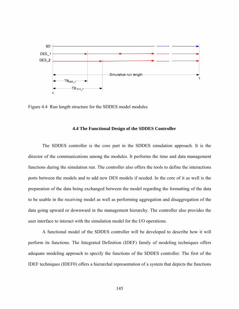
145
Figure 4.4 Run length structure for the SDDES model modules
4.4 The Functional Design of the SDDES Controller
The SDDES controller is the core part in the SDDES simulation approach. It is the
director of the communications among the modules. It performs the time and data management
functions during the simulation run. The controller also offers the tools to define the interactions
ports between the models and to add new DES models if needed. In the core of it as well is the
preparation of the data being exchanged between the model regarding the formatting of the data
to be usable in the receiving model as well as performing aggregation and disaggregation of the
data going upward or downward in the management hierarchy. The controller also provides the
user interface to interact with the simulation model for the I/O operations.
A functional model of the SDDES controller will be developed to describe how it will
perform its functions. The Integrated Definition (IDEF) family of modeling techniques offers
adequate modeling approach to specify the functions of the SDDES controller. The first of the
IDEF techniques (IDEF0) offers a hierarchal representation of a system that depicts the functions

146
done within the system along with relevant inputs needed to perform these functions, outputs
generated upon perfuming the functions, the controls that guide and constrain the functions, and
the mechanisms needed in performing them. The most mature and usable IDEF techniques are
the following: (http://www.idef.com/):
1. IDEF0 for functional modeling to represent functions, activities, or processes in the
system
2. IDEF1 for information modeling to represent the structure and semantics of the
information within the system
3. IDEF2 for dynamic modeling to represent the time varying behavioral characteristics of
the system.
The IDEF0 can be used to model any system that can be viewed as made of “things and
happenings” (Feldmann, 1998). A function is to be represented by a rectangular box that can
have arrows pointing in or out of it as in Figure 4-5. The box can be decomposed into sub
functions that are also represented similarly with the relevant arrows interconnecting the various
boxes in the hierarchical structure shown in Figure 4-6. The methodology is described in details
in the standard documents at the official site for IDEF; Knowledge Based Systems, Inc.
(http://www.idef.com/).

147
Figure 4.5 Generic representation of a function in IDEF0 models

148
Figure 4.6 Hierarchical structure of IDEF0 models

149
4.5 An SDDES Prototype and Case Example
The SDDES will be experimented with using a testbed that will be built for the
experimental part of this research. The SDDES test bed will demonstrate
1. Developing the SDDES simulation modules and model
2. Implementing the SDDES formalism
3. Implementing and evaluating the SDDES synchronization mechanism
4. The functions of the SDDES controller
5. Assessing the usefulness of SDDES

150
CHAPTER 5: THE SDDES SIMULATION FRAMEWORK
The SDDES simulation framework consists of four main processes as shown in Figure 5-
1: modularization, formalization, DES modules resumption setting, and synchronization. SD and
DES modules go through these processes to become modules in the comprehensive SDDES
model of the enterprise system. The SDDES simulation model is managed by the SDDES
controller. This chapter describes the processes and elements of the SDDES framework, but
starts with defining the scope of the manufacturing enterprise as the basis for building the
simulation model.
Figure 5.1 The SDDES framework for simulating the manufacturing system

151
5.1 Scope of the Manufacturing Enterprise System
The SDDES offers a framework for modeling the manufacturing enterprise in a holistic
system perspective (the SD contribution) while utilizing the effectiveness of the DES detailed
approach at the operational managerial level. The main purpose of the SDDES model is the
design and testing of management policies to confirm the estimated performance and expected
behavior based on a comprehensive enterprise-wide feedback. Policies and plans are usually
concerned with resource allocation and utilization decisions and actions. This involves all levels
of management. Testing of plans comprehensively is critical to ensure realizing their outcomes.
For launching a process improvement or a total quality program, enterprise-wide assessment and
involvement are important. In addition, the model can be used as a comprehensive performance
measurement system. Helal and Rabelo (2004) discussed the potential of using SDDES for
building dynamic balanced scorecards. Based on that we recognize the following as the key
components of the manufacturing enterprise model:
1. The internal supply chain of the manufacturing enterprise
2. Strategic decision related business units: resources allocation, rewarding systems,
demand, financial measures, marketing, forecasts …etc.
3. External market and economy indicators
4. Suppliers as external aggregate indicators: supplier reliability index, supplier capacity,
quality, costs, etc.
5. Customers as external aggregate indicators: demand levels, demand variation, satisfaction
level, etc.

152
The internal supply chain represents the flow of materials within the system. As shown in
Figure 5-2, it involves the activities related to the physical flow of materials and/or components
from the external sources through the system until they are converted into finished products that
are supplied to the market to satisfy customers’ needs. Supporting functions include capacity
management, marketing and sales, customer order and backlog management, forecasting, and
inventory management. Inventories are more involved in the actual execution of the production
activities than other supporting functions.
Figure 5.2 Core functions of internal supply chain of the manufacturing enterprise
Figure 5-3 shows the functional structure of the internal supply chain of the
manufacturing enterprise and includes main supporting functions. The units included in this
figure relate to the main flow networks that make up the enterprise system. The enterprise system
consists of the overlapping set of networks of materials (physical goods; raw materials, final
products, finished products, etc), orders (internal and external orders for goods, new employees,
support, etc.), personnel (people as countable individuals), capital equipment (factory space,

153
tools, production and other capital equipment), money (money in the cash sense), and the
information network that interconnects the other networks. Information flows to other networks
to impend decisions in these other networks. The rectangles in Figure 5-3 represent the materials,
order, personnel, and equipment networks of the system. The other layers above the physical
aspects include the resource allocation financial functions, which is more strategic in nature.
Other sections include new product development that includes the research and development
units. The model also should show the revenues and growth and market share related measures.
Market and market share sub model include the advertising, sales, and customer relation
management. It also acknowledges the status of the product in the market. It monitors the level
of attractiveness of the product and the change in product life cycle to estimate the demand.
When the information and money networks are added the scope of the enterprise simulation
model can be represented as in Figure 5-3.
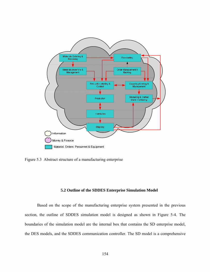
154
Figure 5.3 Abstract structure of a manufacturing enterprise
5.2 Outline of the SDDES Enterprise Simulation Model
Based on the scope of the manufacturing enterprise system presented in the previous
section, the outline of SDDES simulation model is designed as shown in Figure 5-4. The
boundaries of the simulation model are the internal box that contains the SD enterprise model,
the DES models, and the SDDES communication controller. The SD model is a comprehensive

155
model of the enterprise system. The DES models are developed for functions and parts of the
system where detailed analysis is required; mostly at the operational level. The SD and DES
models are interfaced in SDDES. They are treated as modules; each contributing to the
comprehensive model of the manufacturing enterprise system. The SDDES may be made to
interact with the enterprise’s database (e.g. ERP). The communication controller is the core
component of the SDDES approach. It coordinates, synchronizes, and controls the interactions
among the models. The functions of the SDDES controller are described later in this chapter.
Figure 5.4 Outline of the hybrid SDDES enterprise simulation model
5.3 The Modular Structure of The SDDES Model
It is desirable to work with less complex simulation models. Objectives of modeling,
however, dictate the level of details in a model. Less detailed models are easier to build and less

156
expensive. Still, more detailed and refined models are needed to capture the complex dynamics
in the real system units requiring that level of resolution for valid representation of their
functions. SDDES promotes a modular, hierarchical structure of simulation models that consists
of modules of different complexity levels, to minimize the complexity of the simulation model as
a whole and validly capture its structure and dynamics. The modular structure can simplify the
model building processes since relatively smaller modules of narrow scope need to be built.
Several such modules interfaced together result in a comprehensive model. A modular
simulation model is extensible and easy for communication and teamwork development.
The module is a simulation model of a certain system unit. It has a specific function and
thus identifiable sets of inputs and outputs. Modules of the SD and DES components of the
SDDES model are described in the next sections.
5.3.1 The SD modules
Each SD module is a unit in the comprehensive SD part of SDDES. An advantage of the
SD methodology is having generic constructs that are usable for different system and
applications. One such constructs is the SMM (Sterman, 2000) that offers a flexible template for
molding various business and non business system units. The stock management model can
guide the process of breaking down an existing model as well as the building of new SD
modules. SMM was discussed in Chapter 2.

157
The process for developing SD modules for SDDES is shown in Figure 5-5. An existing
SD model of the enterprise can be broken down into modules that have recognizable boundaries
to represent the functional units or the scopes of decision making for the various decisions
makers. Inputs and outputs of each module should be identified to assess the goodness of the
module definition. The process is iterative. Narrow scopes of the modules are preferred to
simplify model maintenance and use. Each module is to perform a certain function or to
correspond to the organizational structure of an enterprise unit.
The module inputs are variables that are not normally under the control of the process
owner of the process represented by the module. Inputs can be from any other module in the
simulation SDDES model. Outputs are offered to the other modules. Once defined, modules are
formalized according to the SDDES formalism, which is presented later in this chapter.
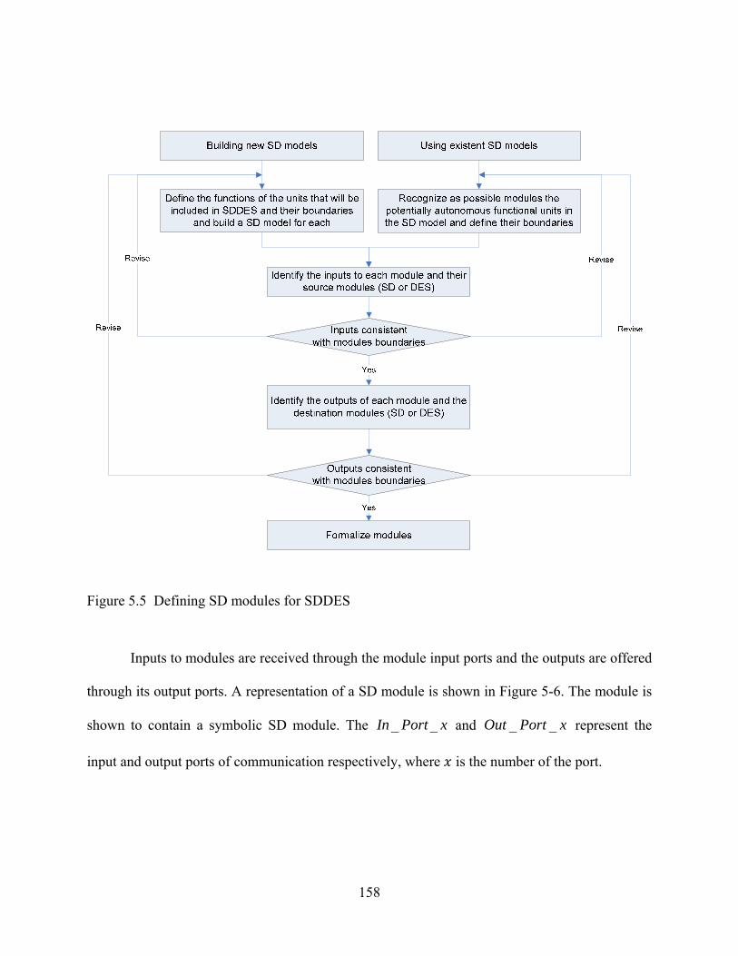
158
Figure 5.5 Defining SD modules for SDDES
Inputs to modules are received through the module input ports and the outputs are offered
through its output ports. A representation of a SD module is shown in Figure 5-6. The module is
shown to contain a symbolic SD module. The xPortIn __ and xPortOut __ represent the
input and output ports of communication respectively, where is the number of the port.

159
Figure 5.6 Symbolic representation of an SD module
5.3.2 The DES modules
Depending on the needs of the decision makers, DES modules are developed to be
interfaced with the SD modules. DES modules can interact with each other as well. The DES
modules are complete discrete simulation models that can be of narrow scopes. A process to
develop the DES modules for SDDES model is shown in Figure 5-7. Module inputs and outputs
should be identified along with the other modules it will interact with. Modules are then
formalized according to the SDDES formalism.
Supply On Order StockOrder Rate Acquisition Rate Loss Rate
Acquisition Delay+
-
++
Adjustment forStock level
Adjustment forSupply On Order
level
Desired Stock
Time toadjust Stock
Desired SupplyOn Order
Time to adjustSupply On Order
Expected Loss Rate
IndicatedOrders
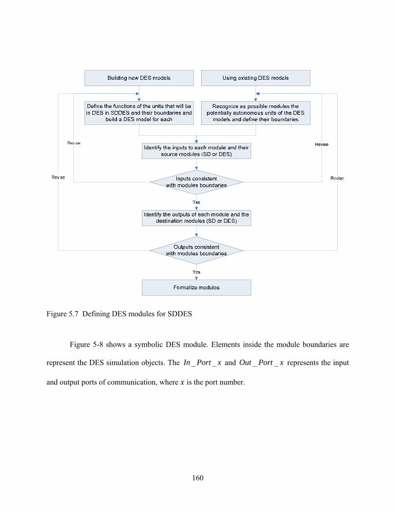
160
Figure 5.7 Defining DES modules for SDDES
Figure 5-8 shows a symbolic DES module. Elements inside the module boundaries are
represent the DES simulation objects. The xPortIn __ and xPortOut __ represents the input
and output ports of communication, where is the port number.

161
Figure 5.8 Symbolic representation of a DES module
5.3.3 Which simulation paradigm should be used to which business unit
The literature review and discussion made in Chapter 2 of SD’s and DES’ views of the
world, potential, and applications in the manufacturing domain support the following criteria to
guide the decision on which business units should be modeled by which simulation technique.
This four-aspect decision criteria (See Figure 5-9) essentially recognizes the perspective within
which the objective of simulating a system is defined and then analyzes three main system
characteristics to assess which simulation paradigm can best meet the simulation objective. The
various business units should be assessed with respect to each of the four aspects.
• Perspective: This implies the objective of simulating the business unit. An analytic
perspective with an emphasis on the detail complexity of the system is more consistent
with using DES. A holistic perspective with an emphasis on the dynamics complexity of
the system is more consistent with using SD.

162
• Resolution: This refers to the contents and structure elements of the system given the
perspective defined above. The system that promotes the individuality of its contents and
structure elements is more consistent with using DES. The system that shows emergent
behavior and emphasizes homogenizing its contents is more consistent with using SD.
• Nature: This describes the nature of the system behavior in reaction to exogenous or
indigenous influencers. The system that behaves stochastically where randomness is
emphasized is more consistent with using DES. The system that behaves
deterministically is more consistent with using SD.
• State Change: The system whose state changes discretely due to countable timeless
occurrences at specific points in time is more consistent with using DES. The system
whose state changes continually, essentially due to time progress is more consistent with
using SD.

163
Figure 5.9 Which simulation paradigm to use to model manufacturing system units
The decision to use DES or SD to model a business unit system is still subject to the
feasibility constraints in terms of the data, financial, and time resources availability. Once built
and validated, all DES and SD models can be interfaced according to the SDDES framework in
order to develop a comprehensive simulation model. Besides flexibility, SDDES can overcome
some feasibility limitations.

164
5.4 The SDDES Formalism
Formalisms are conventions of communications to provide abstraction of systems
elements. The set theory provides the basis of abstraction (Fishwick, 1995). The SDDES
formalism is a generic description of the SDDES modules. The formalism, based on set theory, is
an abstract description of the modules. It offers a format to prepare for the interactions among
modules and a language for modelers and users to interact with the SDDES model through the
SDDES controller and among themselves as well. The structure of the SDDES formalism
contains generic representation of each module type, inputs, outputs, and the formatting and
timing functions.
Three sets and two descriptive elements are needed to describe a SD or a DES module in
SDDES. A SDDES module; m, is described as in equation (17).
),,,,( TBPYXm Τ= (17)
where:
• Τ : type of the module; { }DESSD,=Τ
• X : set of module inputs. For modulem, X is defined by equation (18).
{
{ } }mmmsmss
mmssm
PUOutPortsopmMmaPviMmUopmvimX
⊂∈−∈∈∈=
,, ,,|),,,,(
(18)
where:
o m: current module

165
o vi: the input variable
o sm : the source module, from which viis obtained
o msop : the output port in sm through which vi is given
o mU describes the users of input variable vi in the m. An element in mU specifies
an input port in m, the variables in m that will use vi, timing of needing vi, and
the formatting required in vi. mU can be described as in equation (19)
( ){ }mmm PuInPortsipftuipU ∈∈= ,|,,, (19)
where:
ip : the input port in mthrough which v is obtained to be used u
u : a variable in m that needs to use v
t : timing of reading v into m to be used by u .
f : data preparation action needed for v before it is usable by u .
mInPorts : set of all input ports of m
o M : set of all modules in SDDES model.
o aP: set of all variables in M less the current module; UM
miimPaP
≠=
=,1
o mP : set of all variables in m

166
• TB : time bucket of the module. It indicates the run segment length of a DES module and
in case of a SD module it is set to CONT, for continuous, to represent the entire
planning horizon. As shown later in this chapter, DES modules are run for different run
lengths whereas SD modules are run for the entire planning horizon.
• P : set of all variables in the module.
• Y : set of module outputs; defined by equation (20) for modulem:
{ }{ }mMDPvoOutPortsopMmDvoopmY YmmmYmm −⊂∈∈∈= ,,,|),,,( (20)
where:
o op : the an output port in m
o vo : output variable given through op
o mOutPorts : set of all output ports in m
o YmD : set of destination modules receiving vo . An element in YmD consists of the
destination module identifier and the set of variables in the destination module
that will use vo , as described by equation (21).
{ }{ }mdmddmddYm PVmMmVmD ⊂−∈= ,|),( (21)
where:

167
dm : destination module receiving vo
mdV : set of variables in dm that will use vo . More than one variable in
dm module can use vo ; each may have different timing and formatting
requirements. An element in mdV consists of the variable that will use vo ,
the input port in dm that it will receive vo through, and the timing and
formatting settings, as represented by equation (22).
( ){ }mdmdmdvvmdmd InPortsipPuftuipV ∈∈= ,|,,, (22)
where:
• mdip : input port in dm through which vo in obtained
• vu : variable in dm that will use vo
• mdP : set of all variables of dm
• mdInPorts : set of all input ports of dm
• t : timing of needing vo by vu
• f : data preparation action needed for vo before it is usable by vu
The timing and formatting settings for exchanging data between modules should be
specified by the modeler for each input or output variable. Timing of data exchange is generally
based on the TB settings for the DES modules. Let the SDDES simulation run length be . The

168
SD module run is equal to in length. The DES modules on the other hand are run for segments
each of lengthTB , where TB can be different for the different DES modules. Data exchanges
between modules are carried out between segments. Exchanging data can be at the beginning or
the end of a segment. Frequency of data exchange transactions is a modeling decision based on
the nature of the system being modeled. Data transactions at simulation run startup are used to
initialize the modules. Data transactions at the end or beginning of a segment are used to
exchange input and output data according to the designed feedback relationships. Timing settings
for exchanging the variables include the following:
STARTUP Data transaction at simulation run startup STARTTB _ Data transaction at the beginning of a DES segment ENDTB _ Data transaction at the end of a DES segment
Data preparation and formatting in the SDDES formalism implies transforming the data
from DES or from SD to a format usable in the other paradigm as is explained in Section 5.6.
The whole SDDES model is described to consist of the sets of model inputs, model outputs,
modules included in the model, and the active synchronization mechanism as can be represented
by equation (23). The sets of inputs and outputs in equation (23) refer to the user inputs to the
SDDES model and the outputs the user receives from the model.
),,,( σMOISDDES = (23)
where:
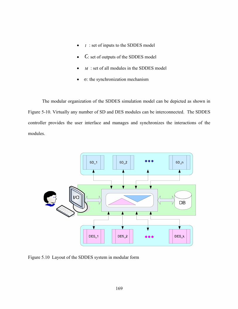
169
• I : set of inputs to the SDDES model
• O: set of outputs of the SDDES model
• M : set of all modules in the SDDES model
• σ: the synchronization mechanism
The modular organization of the SDDES simulation model can be depicted as shown in
Figure 5-10. Virtually any number of SD and DES modules can be interconnected. The SDDES
controller provides the user interface and manages and synchronizes the interactions of the
modules.
Figure 5.10 Layout of the SDDES system in modular form

170
5.5 The SDDES Synchronization Mechanism
In Chapter 3 the review of the existing synchronization mechanisms for hybrid and
distributed simulations showed that the conservative simulation approaches depend on using a
lookahead interval to determine the safe time advancement step. The optimistic approaches use
messages of the timestamps of the events to control the advancement of time and perform
rollbacks when needed. They need events to act and they assume discrete simulations being
synchronized, or a system that is dominated by discrete behavior. Continuous simulation does
not generate events and does not have states that can be defined practically. Synchronization of
the continuous simulations with each other or with discrete models can be approached using TB-
based synchronization methodologies.
In this work we use the concept of the TB in synchronizing the SDDES modules. The
TB is more relevant to running the DES modules and will be used to define the length of the run
segment for each DES module. The SDDES synchronization mechanism requires DES modules
to run not for the entire planning horizon for which the SDDES simulation will be used, but for
run segments. A run segment is a complete discrete simulation run with the needed number of
replications. At the end of the segment the DES modules export outputs to the SD and other DES
modules and receive inputs from them. The choice of the TB size is a modeling decision that is
made considering the desirable levels of accuracy and efficiency as well as the function modeled
in the particular DES module. The SDDES simulation run length L is divided into integer
number of segments for each DES module. The minimum size of TB is the SD computational

171
time step ( tΔ ). For a DES module, mthe length of its run segment is tn
LTB m Δ= , where n is a
nonnegative integer.
Figure 5-11 depicts the synchronization sequence of the SD and DES modules. It shows
the sequence of the SDDES controller actions (numbered as shown on the arrows) in advancing
each simulation module and performing the data exchange. All interactions are executed through
the SDDES controller, which collects the data from all modules and distributes them to the
requesting modules at the time data is needed after performing the needed formatting.
Figure 5-11 assumes three DES modules each with a different TB size. The base TB is
equal to the SD computational time step. The first DES module (TB1 = tΔ ) requires exchanging
data at each SD computational time step. The second DES module (TB2 = 2 tΔ ) is slower than
the first and requires exchanging data every 2 tΔ time units. The third DES module (TB2 = 5 tΔ )
is even slower and requires data exchanges every 5 tΔ time units.

172
tΔ tΔ2 tΔ3 tΔ4 tΔ5 tΔ6
Figure 5.11 SDDES controller’ synchronization action sequence

173
5.5.1 Characteristics of the SDDES synchronization
The following characterizes the SDDES synchronization mechanism:
1. SDDES is a time driven simulation where simulation time is tracked at the SD
module.
2. The SDDES simulation run length is defined at the SD module as the planning
horizon for the enterprise.
3. The SD computational time step ( tΔ ) is the time advance step of the SDDES model.
4. There are no restrictions on setting the SD time step.
5. Each DES module’s run is broken into several run segments. Each segment is a
complete discrete simulation run with sufficient number of replications. Each
segment is initialized with the status of the DES module at the end of the previous
segment in addition to any adjustment received from the other modules.
6. Different DES modules can have different run segment lengths. Run segment length
is equal to tnΔ where +∈ In
7. The shortest DES run segment lengths is tΔ
5.5.2 The SDDES time bucket size
The computational sequence in the SD methodology was described in Chapter 2 as

174
shown in Figure 5-12. All values of system variables are known at the previous time moment; 1t
and given these values the current values at the current time; 2t are calculated. The stock level at
value 2t is the present value of the stock that has resulted from the accumulated difference
between its inflows and outflows. A flow rate value is the present instantaneous value of the flow
between some stocks in the system. Thus the value of any SD variable is its present value
estimated at the current point in time. The calculations sequence reduces the dependence of the
state on the old states.
Figure 5.12 Computational sequence in SD models
Figure 5-13 shows a casual loop diagram portion of a SD model. Production Start Rate is
the rate at which raw materials are removed from parts inventory to start processing. It is also the

175
rate at which raw materials are converted into Work in Process. Work in Process Adjustment,
Finished Inventory Adjustment, and Parts Inventory Adjustment are the amounts of materials
that should be made available to maintain equilibrium. The Indicated Materials Ordering is the
estimated rate of ordering new materials to satisfy the adjustment needs and the scheduled
production rate (not shown). Three balancing feedback loops in the diagram interact to maintain
stable materials supply and production rate.
Figure 5.13 A DES module integrated into an SD model
Assume that the input links of the Work in Process and Production Rate are cut to have
these two variables receive their values from a separate DES module that models the production
processes. The two variables are still used as inputs to some other SD variables. The SD model
sends the Production Start Rate as the input to drive the DES module. At each SD computational
step, the causal loop diagram of SD reacts to the values of Work in Process and Production Rate
by an increase or decrease in Finished Goods Inventory and the appropriate inventory
ProductionStart Rate
PartsInventory
MaterialsOrdering
IndicatingMaterialsOrdering
PartsInventory
Adjustment
Work inProcess
ProductionRate
FinishedGoods
Inventory
+
-
-
+
FinishedInventory
Adjustment
DESWork inProcess
Adjustment

176
adjustments in addition to updating its Production Start Rate. The reaction is communicated to
DES by exporting the new Production Start Rate in expectation of updated Work in process and
Production Rate from DES. Unless DES is able to make these values available at the next
computational step in SD, the feedback loops will be broken and SD will not be able to adjust
itself to maintain equilibrium. Consequently its performance is not easily explained by its
structure and is likely to be erroneous and misleading.
The SDDES synchronization mechanism allows exchanging data between SD and DES at
each computational step. This, however, may be inefficient if the changes in the DES modules
are not as frequent. The choice of the DES segment length should consider the following:
1. It should maintain the integrity of the feedback loops of SD
2. It should maintain the correctness of the SD computations
3. It should capture the changes in the DES modules
Different segment sizes for the different DES modules have the potential of improving
the efficiency of the SDDES simulation model. Depending on the system being modeled,
different segment lengths can be used. For instance, in a manufacturing system early slow
production processes may be modeled by one DES module while the downstream fast assembly
processes can be modeled by a different DES module. If the state of the first (slow changing)
DES module can be considered fixed for more than one SD computational time step then this
module can have a run segment of length tnΔ where n is a non-negative integer. Meanwhile the
other DES module (rapidly changing) may use tΔ as its segment length.
177
5.6 The DES Run Segment Resumption
The SDDES synchronization sequence requires dividing each DES module run into
segments. At the end of each segment the state of part of the system modeled by the DES module
is saved. And at the start of the following segment the saved state is used to initialize the module,
thus the module resumes from where it stopped at the end of the previous segment. Resumption
is vital for the correctness of the results obtained from each DES module after its first segment.
Resumption ensures the following:
1. Each queue at the start of the segment has the same number of entities it had at the end of
the previous segment.
2. Each resource at the start of the segment is in the same state it was at the end of the
previous segment.
3. Entities seizing resource units at the end of a segment continue to seize the same resource
units at the start of following segment
4. Entities that were in processing at the end of the segment and could not finish processing
before the segment ends, continue processing at the start of following using the unused
portion of the processing time
Resumption is performed as described below, for each two consecutive DES segments; k
and 1+k .
1. During segment k :

178
a. When an entity e seizes a resource unit r to start processing, do the following:
i. Record the entity’s identification number
ii. Record the resource unit’s identification number
iii. Record processing time; pt assigned to the entity at the resource unit
iv. Record the time of the processing start event; pspt
b. Purge all recorded values in Step 1-a if entity e releases resource unit r after
processing is completed before the end of the segment
c. When the state of a resource unit r that is not seized for processing or is idle,
changes to an unavailable state, do the following:
i. Record the resource unit’s identification number
ii. Record the state of the resource
iii. Record the time interval; unt , assigned to r for that state
iv. Record the time of event of entering the state; Sunt
d. Purge all recorded values in Step 1-c if time interval unt has elapsed before the
end of the segment
2. At the end of segment k :
a. For each entity undergoing processing save all recorded values in Step 1-a
b. For each resource unit in an unavailable state save all recorded values in Step 1-c
c. For each queue that has a length greater than zero save the number of waiting
entities and their attributes

179
3. At the start of segment 1+k :
a. If saved resumption information in Step 2 are not null then do the following in the
following order:
i. Assign each in-processing entity to the appropriate resource unit using the
information saved in Step 2-a, and let the processing time equal to
)( psptLpt −− where L is the segment length
ii. Set each resource unit in an unavailable state into the same state using the
information saved in Step 2-b, and let the time interval for that state equal
to )( Sunun tLt −− where L is the segment length
iii. Insert entities into the queues they were waiting in at the end of segment
k , using the information saved in Step 2-c
b. Clear all information saved in Step 2
c. Designate the current segment as segment k and return to Step 1.
Figure 5-14 describes the recording and saving of the resumption data from segmentk ,
and use of that data in segment 1+k . This is presented for an entity that starts processing in
segment k and does not finish processing before the end of k and thus needs to continue
processing in segment 1+k .

180
Figure 5.14 Resuming processing between two consecutive DES segments
Figure 5-15 describes the resumption in segment 1+k of a resource unit state that was in
an unavailable state (a failure state) in the previous segment k .

181
Figure 5.15 Resuming the unavailable state of a resource unit between two consecutive DES segments
Processing resumption can accommodate the following cases in the DES modules:
1. A single entity undergoing processing by a single-unit resource
2. A single entity undergoing processing by one unit of a multiple-unit resource
3. A representative entity (batched entities) undergoing processing by a single-unit resource
4. A representative entity (batched entities) undergoing processing by one unit of a
multiple-unit resource
Table 5-1 summarizes these four cases regarding the information to record and save
during and at the end of each segment.

182
Table 5.1 Different cases of processing resumption between consecutive DES run segments
Case To save at end of segment k To do at start of segment k+1
Single entity on a single-unit resource
• Entity id number; e • Resource unit id number; r • Processing time; pt • Processing start time; pspt
• Assign e to r • Processing time = )( psptLpt −−
Single entity on a multiple-unit resource
• For each seized resource unit; i: • Entity id number; ie • Resource unit id number; ir • Processing time; rieipt , • Processing start time rieipspt ,,
• For each seized resource unit; i: • Assign ie to ir • Processing time =
)( ,,, rieipsriei ptLpt −−
Representative entity on a single-unit resource
• Batch id number; b • Batch size; bs • For each entity in b , indexed by i:
o Entity id number; bie • Resource unit id number; r • Processing time; pt • Processing start time; pspt
• Given bs , assign bie ebi to b • Assign b to r • Processing time = )( psptLpt −−
Representative entity on a multiple-unit resource
• For each seized resource unit; i: • Batch id number; ib • Batch size; bis • For each entity in ib , indexed
by j: o Entity id number; bije
• Resource unit id number; bir • Processing time; rbibipt , • Processing start time;
rbibipspt ,,
• For each seized resource unit; i: • Given bis , assign bije to ib
• Assign ib to bir • Processing time =
)( ,,, rbibipsrbibi ptLpt −−
Representative entities may represent entities of the same or different attributes. Batched

183
entities are separated before recording their resumption information. Attributes are recorded
along with the entities’ identification numbers as described in the recoding-saving procedure
above.
5.7 Data Exchanged Between SD and DES
DES modules generate two types of data: observational and time-persistent (Henderson
and Nelson, 2006; Pegden et al., 1992). Observational data are values of random variables that
do not have a life time (e.g. number product units leaving the system). These values are observed
at the occurrence of the relevant events then they expire as the associated entities are discarded
from the system or moved to another state. They can be counted and averaged using simple
arithmetic averaging. A time persistent value is a value of a random variable that is valid from
the event time that generated it until the next event that changes it. An example is the number of
entities waiting a queue.
SD modules are made of two types of variables: stocks and flows. Stocks are
accumulators (e.g. inventory, cash balance) and they continue to exist even when the system
brought to a frozen state. Flows are the rates of accumulating in the stocks or the rates at which
the stocks are depleted. Flows cannot exist if the system is stopped. Flows represent the activities
and policy actions while stocks represent the outcomes of these activities. In SDDES, data from
DES are used in SD and data from SD are used in DES as depicted in Figure 5-16 and explained
in the following subsections.

184
Figure 5.16 Correspondence between SD and DES data in SDDES
5.7.1 Using SD stocks data in DES
SD stocks accumulate units of products, people, orders, etc. Stocks correspond to queues,
buffers, storage areas, and where entities can be held for non-zero time intervals in DES. For
example, the work in process stock in the SD module corresponds to all unfinished product units
in the DES module that are waiting in queues or undergoing processing (delays).
Stocks are not directly measured in time units. They are measured in terms of the units of
their contents. They could have dimensional units such as units/week but this means that the
system is observed for how many units are present in it during the week (Forrester, 1965) that is,
the dimensional units do not represent the flow of the stock contents over a period of time. This
may be called the base time unit in the SD module. The dimensional units of all SD variables
should be consistent. The contents of a SD stock can be exported to queues and delay objects in
the DES modules and they are directly usable in DES.
Figure 5-17 shows a SD module with a single stock of the level of work in process (WIP)
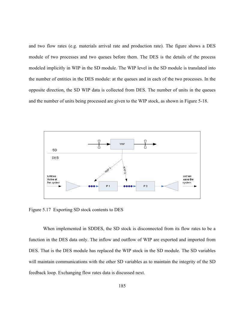
185
and two flow rates (e.g. materials arrival rate and production rate). The figure shows a DES
module of two processes and two queues before them. The DES is the details of the process
modeled implicitly in WIP in the SD module. The WIP level in the SD module is translated into
the number of entities in the DES module: at the queues and in each of the two processes. In the
opposite direction, the SD WIP data is collected from DES. The number of units in the queues
and the number of units being processed are given to the WIP stock, as shown in Figure 5-18.
Figure 5.17 Exporting SD stock contents to DES
When implemented in SDDES, the SD stock is disconnected from its flow rates to be a
function in the DES data only. The inflow and outflow of WIP are exported and imported from
DES. That is the DES module has replaced the WIP stock in the SD module. The SD variables
will maintain communications with the other SD variables as to maintain the integrity of the SD
feedback loop. Exchanging flow rates data is discussed next.
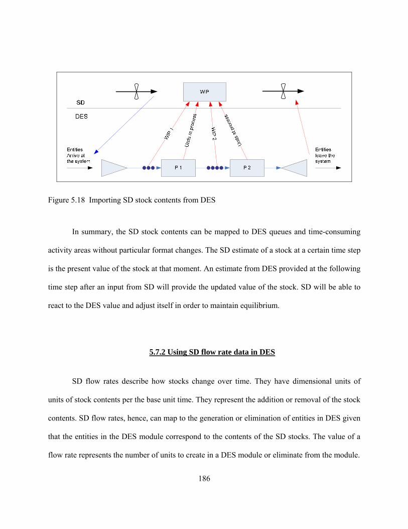
186
Figure 5.18 Importing SD stock contents from DES
In summary, the SD stock contents can be mapped to DES queues and time-consuming
activity areas without particular format changes. The SD estimate of a stock at a certain time step
is the present value of the stock at that moment. An estimate from DES provided at the following
time step after an input from SD will provide the updated value of the stock. SD will be able to
react to the DES value and adjust itself in order to maintain equilibrium.
5.7.2 Using SD flow rate data in DES
SD flow rates describe how stocks change over time. They have dimensional units of
units of stock contents per the base unit time. They represent the addition or removal of the stock
contents. SD flow rates, hence, can map to the generation or elimination of entities in DES given
that the entities in the DES module correspond to the contents of the SD stocks. The value of a
flow rate represents the number of units to create in a DES module or eliminate from the module.

187
In Figure 5-18, the inflow to the WIP stock (materials arrival rate) is directed to the DES
module. Materials created at DES based on the inflow rate will be waiting in queues, in
processing, or will leave the system when they are finished. As the entities leave the system they
are counted and their count over the segment duration will make the DES value for the SD
outflow rate. Given the base time unit of SD and the computational time step size, the value of a
flow that is to be exported to a DES module at the current point in time t should be scaled to
match the DES run segment length such that the value itself without the time dimension can be
used. If the run segment length is tnTB Δ= , then a DES equivalent of the SD flow rate variable
is calculated by equation 24 where tΔ is the SD computational time step.
⎟⎟⎠
⎞⎜⎜⎝
⎛ Δ=
UnitTimeBaseSDtn
___ valuerate flow SDrate flow SD of equivalent DES (24)
5.7.3 Using DES observational data in SD
Observational data exist in the DES modules only for the duration of the event that
created them, which is zero. Observational data can be mapped to flow rates in SD. Mapping to
stocks requires time-persistent data. For dimensional correctness in SD, observational data
should be transformed into equivalent quantities that can be measured in the same units of the
flow rates they map to. Counted over the duration of the run segment, the DES observation data
can map to an equivalent SD flow rate using equation 25.

188
⎟⎟⎠
⎞⎜⎜⎝
⎛ Δ=
UnitTimeBaseSDtn
___count DESdata counted DES of equivalent SD (25)
Let X be the random variable of the number of entities removed from a system modeled
by DES. At the event times of removing the entities X may take the values of x1, x2, x3, … etc.
at the event times t1, t2, t3, … respectively (Figure 5-19). To estimate a removal rate from DES
the number of entities over the in-between events times is divided by the time interval length.
The rate estimates are denoted by SDX in Figure 5-19. Assuming the DES model started idle and
empty at time zero, then the system needed t1 time units to deliver x1 entities. The equivalent rate
over t1, 1SDX is estimated as the ratio of x1 to t1. Rates over other periods are estimated similarly.
When exported to a SD module, the estimated equivalent value over each time interval is used
for the appropriate SD flow rate variable.

189
Figure 5.19 Mapping observational data from DES (top) to equivalent rate variables in SD (bottom)
5.7.4 Using DES time-persistent data into SD
DES time persistent data are usable in SD as they are generated in DES and they can map
to the SD stocks. Both time-persistent data and SD stock contents data represent quantities that
stay valid over nonzero time intervals. The time-persistent values are recorded at the times of the
events that affect them. More than one event can occur during the DES run segment that affect

190
the time-persistent value. The end-of-run DES value of the time-persistent variable maps to the
appropriate SD stock level at the same point in time.
It is also possible to estimate a time-weighted average of the DES time-persistent variable
over the DES run and export it to the SD. In this case the average value may not be usable for a
stock level. Such a DES value can add more information to the SD module. For instance, if the
work in process data is collected from a DES module, the level of work in process at the end of
the DES run corresponds to the relevant SD stock. Whereas a weighted average value of the
work in process over the DES run can be used to indicate the level of system crowdedness,
which can be used to estimate a labor satisfaction measure, or an indicator of the shop floor
quality of environment. Assuming a DES segment length of tΔ , Figure 5-20 illustrate these two
approaches. Some accuracy analysis will be needed since the weighted-average value will
correspond to somewhere between the begin and end of the SD computational step. The SD
theory calculates the stock level at the end of the time step, which is used in the experimental
analysis in the next chapter.
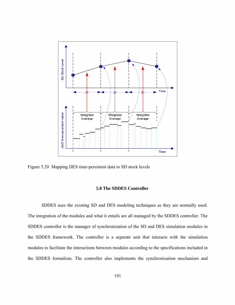
191
Figure 5.20 Mapping DES time-persistent data to SD stock levels
5.8 The SDDES Controller
SDDES uses the existing SD and DES modeling techniques as they are normally used.
The integration of the modules and what it entails are all managed by the SDDES controller. The
SDDES controller is the manager of synchronization of the SD and DES simulation modules in
the SDDES framework. The controller is a separate unit that interacts with the simulation
modules to facilitate the interactions between modules according to the specifications included in
the SDDES formalism. The controller also implements the synchronization mechanism and

192
provides the user interface to perform I/O operations and to define/modify/replace the modules
or the model or management policy settings.
Figure 5-21 represents the position of the controller between the SD and DES modules
and the flow of data from and to the modules through the aggregation/disaggregation functions
(symbolized by the up and down triangles). The SDDES controller reads data from all modules
and formats the data as described in Section 5.7, before they are sent to the requesting modules.
And it keeps track of the simulation time.
Figure 5.21 The SDDES controller directions of exchanging data
The SDDES controller acts in the following areas:
1. Data management: The controller ensures that the information indicated in the
definition of the SD and DES modules (in their formalism specifications) are executed

193
properly regarding formatting and timing. It also allows users to modify the model
settings.
2. Time management: The controller implements the synchronization mechanism and
keeps track of the simulation time. The DES modules do not run for the entire SDDES
simulation run length. The controller estimates the time for each with respect to the
overall SD modules such that a user can observe the correct simulation time.
3. Participation management: The controller offers the functionality needed to add new
modules to the SDDES model as well as to modify or replace existing modules. This is
achieved through providing and or modifying the module data according to the SDDES
formalism.
5.8.1 Functional model of the SDDES controller
To describe how the SDDES controller will perform its functions, we develop an IDEF0
model of it. The functional model describes how the controller manages the SDDES simulation
run. The IDEF0 method offers a hierarchal representation of a system that depicts the functions
done within the system along with relevant inputs needed to perform the functions, outputs
generated upon perfuming the functions, the controls that guide and constrain the functions, and
the mechanisms needed in that. The basic model as shown in Figure 5-22 is presented from the
point of view of the modeler/user of the SDDES. A single box is used to indicate the function of
the controller, namely executing the SDDES model run. The sets of inputs, controls, outputs, and

194
mechanisms (the ICOMs) used in the A-0 model are described in Table 5-2.
Figure 5.22 A-0 IDEF0 functional model of the SDDES controller

195
Table 5.2 ICOMs for the A-0 IDEF0 model of the SDDES controller
Inputs
I1 Operational settings
Characteristic information representing the current status of the system. They are elements of the management policies that will be tested and evaluated with the simulation model. The module parameters are assigned values in this action. These values are provided by the modeler or obtained from the active information system (M2).
I2 Modules settings
The inputting of the data required by the SDDES formalism. Modules can be modified, deleted from, or added to the model.
I3 Run settings Specifying the planning horizon, number of replications for the DES modules, as well as the time units and needed parameters that will be monitored. Also the outputs that are of interest are specified here
Controls
C1 SDDES formalism
This guides the addition, modification, or deletion of modules. Also specifies the data needed to set the model and the run.
C2 SDDES synchronization
This is SDDES synchronization algorithm. It guides the simulation run and the data exchange transactions.
Outputs O1 Performance indicators
This is the regular outputs of a simulation model
Mechanisms
M1 Modeler Represents the user of the simulation model in general. The modeler performs all I/O operations
M2 Info system This is the existing information system of the company (e.g. ERP or MRP). Module variables are linked to data provided by the information system. Outputs can also be added to the information system.
M3 GUI The graphical user interface is an integrated unit of the controller. It offers several user interfaces through which the modeler interacts with the controller and the model.
M4 Modules These are the module information saved in their files (e.g. the Arena and Vensim files in the current work). They are called to be used as necessary by the modeler and during the run for sure.

196
The controller executes the SDDES simulation model using these sets of inputs, controls,
outputs, and mechanisms. The modeler uses the appropriate user interface to input module data
or the simulation data. The modeler also observes the simulation outputs to assess the need to
modify the plans and policies being tested. The inputs provided by the modeler are specified by
the two controls; the formalism and the synchronization algorithm. The controller uses a
database to store the input data and the ongoing outputs during the run. To set the modules, the
controller extracts the parameters of the modules (via calling M4) such that the modeler would
assign values to them or link their values to the appropriate data in the information system.
The A-0 diagram is decomposed into more detailed definition of the controller functions.
The A0 diagram of the IDEF0 model is the first level of details of the function described in the
A-0 model. A0 for the SDDES controller models the three basic functions of the. In the IDEF0
terms these functions are the A1, A2, and A3 in Figure 5-23. Each of these functions is
decomposed further as necessary to offer a complete description of the controller role in the
SDDES model, prior to its implementation. The A0 model is describe in Figure 5-23 and
explained afterward.

197
Figure 5.23 The A0 IDEF0 model of the SDDES controller
The Interact With User function (A1) allows the user (the Modeler in the above model) to
perform I/O operations as well as defining the modules. The appropriate GUI is initiated for the
Modeler to input the necessary settings. These inputs are communicated to A2 and A3 for the
models to be defined and the run to be ready to be executed. The GUI is developed to meet all
use cases of the system and these use cases are controlled by the SDDES formalism (adding or
deleting modules), by the current contents of the saved modules (coming from A3 to modify
modules, assign input values to their variables, etc.), and by the performance indicators (coming
from A2 for the user to observe outputs and do necessary adjustments when desirable).
The Manage Model function works to accept changes in the existing modules and add
A1
Interact With User
A2
Manage Simulation Run
A3
Manage Model
I1 Operational settings
M1 Modeler
C2 SDDES synchronizationalgorithm
Simulation run info
C1 SDDES formalism
Module contents
M4 Modules
SDDES / A0 The SDDES Controller
O1 Performance indicators
O1 Performance indicators
M3 GUI
Run database
Module contents
Current simulation
time
I3 Run settings
I2 Module settings
Modules specifications
M2 Info systen

198
new ones to the SDDES model as inputted by the modeler in A1. The modules are saved in their
simulation software files and the files are called as necessary (M4). The current contents of the
modules are the outputs of A3 that are fed back to A2 so that the controller reads the TB setting
for the modules and the defined data exchange transactions that will be executed during the run
in the A2 function. The synchronization algorithm (C2) controls A2 along with the relevant
information from the formalism (C1). The current module contents from A3 are also fed back
into A1 for the Modeler to correctly assign the operational and run settings.
The output of A2 is the output of the simulation run, which is offered as the overall
output of SDDES and is fed back to A1 for the modeler to analyze the performance with the
appropriate GUI. It is noted that the A2 function is internal; no direct user interactions are
needed with it. During the run, the behavior of the system is feedback to A1 for the user to
perform any adjustment if desirable.
The output of A1 is the simulation run info representing the settings needed to start the
simulation run at A2. These ongoing outputs are saved in the run database and are as appropriate
during the run. Of particular importance, the results of the run segments of the DES modules are
saved to be used in the following segments as described by the DES resumption algorithm.
A detailed IDEF0 model of the A2 function in Figure 5-24 is given in Figure 5-25. The
core of this function is to implement the synchronization algorithm (A2-2), given that the all
modules have been formalized and that the resumption specifications have been defined for the
DES modules. This data is represented by the simulation run info input to A2-2 module in Figure
5-24. Settings (SD run settings and DES run settings) for each module are forwarded to the

199
modules. The SD module is set to reflect the management strategies and policies using the inputs
of market demand, investment and resource allocation related decision and the enterprise
financial indicators. Outputs of running the SD module (A2-1) are exported to the DES module
via the A2-2 module. They include the decisions regarding the scheduled production, and
adjustments for current capacity in addition to desirable performance levels. Upon running the
DES modules (A2-3) the outputs (Operational performance measures) are sent to the A2-2 for
formatting to be forwarded to A2-1. The overall SDDES model outputs are the system
performance measures (O1) as was described earlier in Figure 5-23.

200
Figure 5.24 IDEF0 model of the SDDES controller function of managing the simulation run
5.9 SDDES Test Bed
This SDDES test bed is an implementation of the SDDES controller and is used for the
experimental analysis and testing of the SDDES simulation framework. A Visual Basic (VB)
application was built that communicates with the Arena and Vensim software packages. Arena
was used to build DES modules for a manufacturing system as described in Chapter 6, while
Vensim was used to build the SD modules of the same system. The VB implementation of the

201
SDDES controller uses the ActiveX Data Object (ADO) technology to connect to the simulation
engine in Arena to gain access to and control the simulation modules. The functions and
messaging tools of the Vensim’s Dynamic Link Library (DLL) are utilized to communicate with
the SD modules while establishing a Dynamic Data Exchange (DDE) link to have the software
acting as a server/client application for the data exchange operations. To use it as the centralized
data repository, the controller uses the ADO of the MS Excel application object to perform the
data preparation operations and appropriately authorize the simulation engines to perform data
read/write operations. The modeler interacts with the VB application to perform the input/output
operations before and while the model run. A schematic diagram of the structure of the test bed
implementation of the SDDES controller is shown in Figure 5-25.
Figure 5.25 Schematic diagram of the SDDES controller test bed implementation
The VB code listing of the implementation of this test bed and simulation models
202
described in section 6.1 in the next Chapter are available.
5.10 Chapter Summary
This chapter presented the conceptual design of the SDDES hybrid simulation
framework. It presented the overall structure of the SDDES model and its coverage in modeling
the manufacturing enterprise system and introduced and explained the concepts and components
of the simulation framework. The concepts presented in this chapter are the following:
1. The scope of the manufacturing enterprise system
2. The modular structure of the SDDES simulation framework
3. The SDDES synchronization and controller actions sequence
4. The segmentation of the DES simulation runs
5. The DES run segment resumption algorithm
6. The SD and DES data formatting
7. The functional model of the SDDES controller
203
CHAPTER 6: EXPERIMENTAL ANALYSIS
This chapter consists of four parts. Part one demonstrates implementing the SDDES
hybrid simulation framework to build a simulation model of a local manufacturing company. It is
based on using the test bed described in Chapter 5. Part two presents a case of using an SDDES
simulation model to analyze the manufacturing value chain. Part three compares SDDES to
AnyLogic. Part four discusses the potential of using SDDES in the real time control applications
of the manufacturing system.
6.1 Using SDDES to Model The Manufacturing System
This section describes using the SDDES simulation methodology. A case in which an
SDDES hybrid simulation model is built for a real manufacturing system is used to describe the
implementation and use of the concepts and elements of the SDDES framework. The objective
of the case is to demonstrate the validity of the SDDES methodology as described in Chapter 5
and its ability to integrate the SD and DES paradigms and build usable comprehensive hybrid
simulation models of the real manufacturing systems.
The implementation of the SDDES methodology will use the test bed described in section
5.9. SD and DES modules will be built to represent the manufacturing system of a local optical
204
product manufacturer (will be referred to as PMOC Inc). The modules will be synchronized
using the SDDES controller test bed. The module definition and building, resumption setting,
and module formalizing processes will be described.
6.1.1 PMOC Inc.’s lenses manufacturing system
PMOC; a local manufacturing company, engages in the design, development,
manufacture, and distribution of optical components and assemblies. The company offers
families of precision molded glass aspheric optics – isolators, fiber optics collimators,
GRADIUM glass, and other optical materials for laser and light control products. The company
offers its products to various markets including industrial, medical, defense, test and
measurements, and communications markets. The precision molded optics (PMO) process
produces lenses for industrial laser and other optical applications and is the focus of the
simulation model. Lenses production is the oldest product line at PMOC. Figure 6-1 shows a
high level organizational structure of PMOC.

205
PMO TechnologiesPresident & CEO
Marketing VP
Operations VP
Sales VP
Finance & Admin VP
Facilities & Equipment
HR
Accounting
IsolatorsAssembly
Collimators GRADIUM Product Engineering PMO
ManufacturingOperations
support
PMO
Preforms
Figure 6.1 PMOC high level organizational structure
PMOC has a stable PMO customer base of about 1700 customers. The company has
established long term relationship with its customers by providing customized products. Systems
using PMOC’s lenses at customers’ facilities had been designed to use PMOC’s products. With
special requirements in lenses in addition to high quality level and support, customers have been
willing to pay a premium for PMOC’s product. This has helped The Company maintain a stable
market share over the past few years despite using an old manufacturing technology with limited
capacity.
Rapid technological advances and growth in the optical market (at the industrial and
consumer electronics levels) challenged PMOC’s strategy of relaying on providing customized
products to loyal customers. Customers renovating optical systems are considering switching to

206
competitors who can offer similar variety and quality at cheaper prices. Recognizing the limits of
its production capacity and technology and with the expected success and more promising
markets for other products, PMOC is planning no investments in its PMO production line and is
investigating an outsourcing decision. In this section we describe building an SDDES simulation
model of PMOC’s PMO operations that can be used to assess the system capabilities and ability
to maintain its performance.
6.1.2 Building the SDDES hybrid simulation model
The objective of the model is demonstrating the implementation of the SDDES
simulation framework and its potential for modeling the manufacturing system and explaining its
behavior and level of performance. SD and DES simulation models were built to be used as
modules in the SDDES model. The SD and DES modules were built as regular SD or DES
simulation models. We then followed the module definition processes described in Chapter 5
(See Figure 6-2 below) to develop them as modules. Defining a SDDES module is essentially
defining its sets of inputs and outputs and then formalizing it. Formalizing the module as
described in the SDDES formalism includes the definition of the resumption (for DES modules)
and synchronization (data exchange timing and formats) settings for each module.

207
Figure 6.2 Defining an SDDES module of an SD or DES model
The following steps were followed to build the SDDES model:
1. Defining the scope and contents of the model
2. Defining the boundaries of each module
3. Building the SD and DES modules
4. Validating the modules
5. Defining the inputs and outputs for each module
6. Defining the DES modules resumption settings
7. Defining the modules synchronization settings
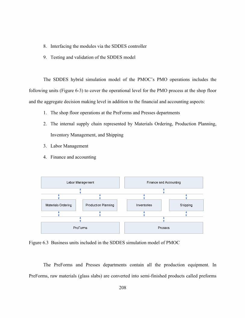
208
8. Interfacing the modules via the SDDES controller
9. Testing and validation of the SDDES model
The SDDES hybrid simulation model of the PMOC’s PMO operations includes the
following units (Figure 6-3) to cover the operational level for the PMO process at the shop floor
and the aggregate decision making level in addition to the financial and accounting aspects:
1. The shop floor operations at the PreForms and Presses departments
2. The internal supply chain represented by Materials Ordering, Production Planning,
Inventory Management, and Shipping
3. Labor Management
4. Finance and accounting
Figure 6.3 Business units included in the SDDES simulation model of PMOC
The PreForms and Presses departments contain all the production equipment. In
PreForms, raw materials (glass slabs) are converted into semi-finished products called preforms
209
(glass balls). Raw materials arrive in the form of slabs of 4 by 6 inches and 1 inch thick. Slabs
are inspected for physical defects and thermal expansion characteristics and are then sliced into
plates of different thicknesses to meet the different sizes of the various types of final product.
Plates are formed into glass balls (preforms) of different sizes. Preforms are then annealed,
ground, lapped, polished, smoked and baked, and cleaned before they are sent to the Presses
department for the finishing operations. In Presses, the preforms are pressed on two types of
presses to make usable lenses of different optical characteristics.
The PreForms department uses a relatively old technology. And because of the different
types of final product, the processing times and batch sizes at each processing step vary
significantly. There is a single annealing oven that can process a batch of 1000 to 1500 units
(depending on the size of the raw preforms) per run and it runs for average of 12 hours. There are
four grinding, five lapping, and 15 polishing machines that each can process between 100 and
350 units each run where the processing time vary from 25 minutes to more than five hours. The
smoke and back and wash operations use heat and chemicals to clean the preforms in batches of
up to 100 units and processing times are measured in minutes. There are 13 workers in addition
to the production manager in the PreForms department. Workers are grouped for the different
processing steps yet they are trained to operate all equipment.
The different lens sizes and necessarily the differences in batch sizes and processing
times with the lack of computer control make synchronization critical to ensure the availability
of materials to meet the Presses department requirements. Figure 6-4 shows the daily production
rate of the PreForms department for a six-month period. This shows all types of lenses pooled

210
together. Preforms are stocked at the department until requested by the Presses department
operators.
Figure 6.4 Daily raw preforms output from the PreForms department (actual data provided by PMOC)
The Presses department is run as a pull production system that pulls raw preforms from
PreForms according to the schedule to meet customer orders. Orders arrive in varying sizes for
the different types of lenses. Raw preforms are pressed into final usable lenses at two types of
pressing workstations: the air presses and the Nitrogen (Ni) presses. Each air press has seven
pressing heads, which can be run separately. Each Ni press has six pressing heads, which are also
independent from each other. Air or Ni refers to the technology used in the press where pressing
is carried in a vacuum or within the presence of the inert Ni gas. Each type is capable of
producing certain set of optical characteristics that overlap such that some types of lenses can be
0
500
1000
1500
2000
2500
3000
3500
4000
2/7/20
05
2/14
/200
5
2/21
/200
5
2/28
/200
5
3/7/20
05
3/14
/200
5
3/21
/200
5
3/28
/200
5
4/4/20
05
4/11
/200
5
4/18
/200
5
4/25
/200
5
5/2/20
05
5/9/20
05
5/16
/200
5
5/23
/200
5
PreForms Daily Production ‐ Feb through June 05

211
pressed on either type of press. Each press is run by a single operator. There are nine and seven
Air and Ni presses respectively. After pressing, the operator inspects the lenses before they are
forwarded to the more advanced interferometer testing station where they are accepted or
scrapped. Operators retrieve the preforms daily according to the scheduled production of the day.
Scrap rate is high at Pressing; ranging between 25% and 35% of attempted pressing operations.
Utilizing the decision criteria presented in Chapter 5, the system units indicated in Figure
6-3 were modeled by SD or DES as indicated in Table 6-1. The production processes at the
PreForms and Presses departments are in DES while the rest of the business units are in SD. This
is discussed afterward.
Table 6.1 Classifying PMOC’s business units in the SDDES model as SD or DES models
Business Units
Decision Criteria
Use SD or DES
Perspective Resolution Nature State Change
Hol
istic
Det
aile
d
Hom
ogen
ized
Indi
vidu
aliz
ed
Det
erm
inis
tic
Stoc
hast
ic
Con
tinua
lly
Dis
cret
ely
Production Planning 1 0 1 0 1 0 1 0 SD Materials Ordering 1 0 1 0 1 0 1 0 SD Inventories 1 0 1 0 1 0 1 0 SD Shipping 1 0 1 0 1 0 1 0 SD Labor Management 1 0 1 0 1 0 1 0 SD Finance & Accounting 1 0 1 0 1 0 1 0 SD PreForms 0 1 0 1 0 1 0 1 DES Presses 0 1 0 1 0 1 0 1 DES
We modeled the PreForms and Presses departments using DES to allow for monitoring

212
each individual unit of equipment and synchronizing their performance to ensure smooth flow of
materials in PreFoms and from PreForms to Presses. The high scrap rate can cause occasional
loss of materials and accurate estimates of the scrap rate are necessary. Stochastic behavior due
to varying processing times and batch sizes in addition to scrapping rate is dominant. DES
models can provide good estimates of scrap based on each piece of equipment’s performance.
DES is effective in modeling materials flow between processing steps. Tracking production,
amounts of scrap, and work in process in addition to the equipment failures and the workforce
availability and performance are essential in modeling production lines.
The aggregate production management level, represented by the other units indicated in
Figure 6-3 were modeled using SD. Materials ordering, production planning, inventories, and
shipping represent the internal supply chain of PMCO. Production at the shop floor level is
controlled through the interactions with these functional units. They are managed at the
aggregate decision making level providing planning responsibilities. Customer orders are
received and accordingly needed raw materials, materials usage, and production rates are set.
These decisions use shop floor level data for current production yield, available work in process
and current work load. Individual production equipment units are not monitored at this planning
level. Instead the overall performance of the PreForms and the Presses departments is estimated
and used in the materials ordering and inventory management and production scheduling
decisions. PMOC partners with a single supplier of raw materials that delivers materials on a
monthly basis to cover the monthly demand. Arriving raw materials shipments are always
inspected but rejections never occurred. No particular sources of stochasticity are recognizable

213
when making decisions at this level. PMOC serves a fairly stable customer base. The company’s
strategy is essentially to serve its current customer base. Part of this is due to the limited capacity
and the higher prices than competitors that do not attract new customers. It is also noted that
PMOC is directing resources to other product lines that are more promising and they maintain
PMO production at current stable level without plans for investing in it as outsourcing is being
considered.
Labor attrition is at the low rate of less than one worker per month that is compensated
for by an equivalent hiring rate with cooperation with a hiring agency that provides basic
training. Average employment length is three years. New operators are trained by their
coworkers when they join the workforce such that productivity is not negatively affected by
them. Finance and accounting units monitor performance in financial measures. These are
essentially deterministic business unit given the stable customer base, orders, and market share.
This makes these units candidates for modeling in SD models.
6.1.3 Building the SD modules
The SD modules were built using the standard SD methodology in which reference
modes of behavior and dynamic hypotheses are developed to describe the perceived historical
and projected behavior of the system and the major causal relationships that underlie these
modes. These modes and hypotheses reflect the decision makers’ mental models and perceptions
of the system. They represent the basis for building the stock and flow model, which is then

214
reviewed with them for validity.
We utilized the stock management model (Sterman, 2000) as described in Chapter 2 of
this dissertation in building the SD modules. The stock management model (SMM) provides
abstract concepts of the causal relationships in terms of the stocks and flows variables.
Participants from various departments at PMOC in relation to the PMO manufacturing were
interviewed. Company’s CEO, VP of operations, finance, marketing, and human resources, in
addition to marketing and customer service staff and production managers, were interviewed to
develop the dynamic hypotheses of the modules. Financial data, however, were obtained from
public data posted on the Internet at www.yahoo.com as the company is a public company.
The main factor that shaped the way they managed PMO was the company’s intent to
outsource the process. The company purchased the PMO about ten years earlier for market
diversity to improve their financial performance. PMOC maintained the level of performance
while planning investments in new additional markets and technologies, not including upgrading
PMO manufacturing capacities. Rapid technological advances and changes in the market had
limited PMO’s success. Long term customers continued to partner with PMOC. However,
market share and customer base could not be increased with the limited capacity and relatively
higher prices given the increasing competition and the evolutionary changes in the market. The
company decided to focus on its other markets and not to invest in PMO, which would be a large
investment for an already highly competitive market where competitors are technologically
ahead. For being in a restructure phase, PMOC is a public company that has been experiencing a
decreasing share price (Figure 6-5). This would continue unless the company reorganizes its

215
production lines and direct investments in the more promising markets.
Figure 6.5 Decreasing trend in PMOC market share price - described by PMOC managers and as shown on www.yahoo.com
The objective of the management then was to maintain PMO’s performance and
minimize operational expenses. The main concern expressed by the participants was the high
scrap rate (estimated 25% to 40%). Scrap has been observed to be slightly increasing and as
equipment get older; it was projected to be higher (Figure 6-6). Higher scrap is translated into
lower yield.
Figure 6.6 increasing trend in scrap rate – described by PMOC managers

216
Not only scrapping causes the loss of materials (semi finished preforms) but it can also
cause longer delivery delays (Figure 6-7 a), the need for emergency materials ordering at higher
expenses, and it requires repairing/replacing the metallic pressing head molds which adds to the
production expenses (Figure 6-7 b). The company traditionally offered an average of one week
delivery delay.
Figure 6.7 Deliver delay expected to increase as well as production expenses – described by PMOC managers
The many types of lenses and the varying order sizes for each type create difficulties for
synchronizing the production processes that leads to fluctuating materials and work in process
inventories (Figure 6-8 a). Improving scrap rate would require investments in new equipment to
replace the technologically old, less reliable equipment. PMOC is planning no such investments.

217
The reason behind that is the increasing competition. Competitors offer lower prices than PMOC
which do not have sufficient capacity to increase productivity in order to lower prices. Besides,
the pressing technology is more expensive than the newer ceramic-based presses that competitors
use. Customer orders are expected to decrease (Figure 6-8 b) in favor of faster delivery and
lower prices. More importantly, current customers upgrading their systems that use PMOC’s
products are shifting toward using more standardized competitors’ products at lower prices.
Some Customers have indicated that to PMOC. The company is considering more advertising
but higher precise for many types of lenses do not encourage them. PMOC’s traditionally market
share of about 3% is expected to decrease as its customers start to renovate their equipment.
Figure 6.8 Increase in delivery delay contributes to decreasing customer orders – described by PMOC managers
Each of the business units modeled in SD could be modeled using the SMM. The task of

218
the materials ordering and inventory management is regulating the inventory level by
maintaining a level of materials on order and estimating the appropriate level of adjustment if
inventory is different from its target level. The same regulation task is implemented in the
production planning and shipping unit, which also includes the work in process inventory level.
Figure 6-9 shows the materials ordering and inventory module and the production planning and
work in process module. Together they represent the physical flow of materials from the supplier
to the customer. These are two overlapping SMMs. The first is for raw materials inventory and
ordering (left part of Figure 6-9) consists of the two stocks of Parts On Order and Parts
Inventory, which are regulated by the flow rates of Parts Order Rate, Parts Arrival Rate and
Production Start Rate in addition to the auxiliary variables used to estimated the necessary
adjustments and the indicated parts order rate. The scheduled production rate from the
production planning module (right part of Figure 6-9) is the input that drives the materials
ordering section. Materials are ordered to meet the scheduled production and needed inventory
adjustment.
The Production Start Rate is the rate at which materials are taken from the raw materials
stock (Parts Inventory) to start processing (become work in process). This rate is the link to the
production planning and work in process module, which is the second SMM in Figure 6-9 (right
part). There are three rather than two stocks in this module. Two work-in-process (WIP) stocks
are used to correspond to the PreForms and Presses departments. This production planning and
WIP module regulates the WIP at the two departments to ensure smooth production rate and the
availability of the final products in the Finished Product Inventory stock for shipping.

219
As an SMM, the WIP stocks are regulated through estimating the necessary adjustments
to bring them to the equilibrium level if they are above or below that level. The Finished Goods
Inventory carries the final product prior to shipping to customers. This module is derived by the
customer order rate that is used to estimate the scheduled production rate. Scheduled production
rate is exported to the materials ordering and inventory module. The level of raw materials
inventory (Parts Inventory) is exported to the production planning and WIP module to use it to
start processing. Production start rate is a function of the level of parts inventory as well as the
available production capacity that is imported from the labor management module.

220
Figure 6.9 SD model of the internal supply chain of PMOC Inc.
This model consists of two overlapping SMM constructs. The first is materials ordering and inventory (PARTS ON ORDER and PARTS INVENTORY stocks). The second is production, work in process, and finished product inventory (PREFORMS WIP, PRESSES WIP, and FINISHED GOODS INVENTORY stocks)
PARTS ONORDER
PARTSINVENTORYParts Arrival
Rate
Desired dayssupply of PI
Initial partsinventory
Initial parts onorder
Partsinventory goal
Parts inventorycorrection
Time to correctparts inventory
Parts on ordercorrection
Parts on ordergoal
initial finishedinventory
Time to correctinventory
Finished inventorycorrection
Finishedinventory goal
Averagecustomer order
rate
Desiredproduction
rate
FINISHED GOODSINVENTORY Shipping
Rate
DeliveryDelay
<Supplierdelivery delay>
Yield
Preforms yieldPresses
yield
Indicated partsorder rate
Parts OrderRate
<Effect of suppliercapacity on parts
order rate>
<Effect of cashconstraints on parts
ordering>
<PARTSINVENTORY>
<PotentialProductionRate From
Labor>
ScheduledProduction
Rate
<MaximumCapacity>
PREFORMSWIPProduction Start
Rate
PRESSESWIPPreforms
Production RateProduction
Completion Rates
Preforms cycletime
Presses cycletime
PreformsScrap
Presses Scrap
Initial WIPPresses
Initial WIPPreforms
WIP goalPresses
WIP goalPreforms WIP correction
Presses
Time to correctWIP Presses
Time to correctWIP Preforms
WIP correctionPreforms
Desired ShippingRate
<Preforms cycletime>
<Presses cycletime>
<Supplier deliverydelay>
The COR
<Effect of deliverydelay on market share>
<Finished inventorycorrection>

221
Figure 6-10 shows the labor management module. Two stocks; Labor Being Recruited
and Labor are regulated through four flow rates. This module uses the scheduled production rate
from the production planning and WIP module to estimate the needed level of capacity including
overtime when necessary. The module indicates the need to recruit new worker if scheduled
production increase to justify that (and if financial resources support hiring). This is managed by
using the needed capacity, available, and scheduled production rate to estimate the corrections to
labor and labor being recruited stocks. This indicates the labor recruiting rate. Labor being
recruited moves to become labor (get hired) after some hiring delay, according to the labor hiring
rate. Labor then bay be fired or they leave voluntarily. The available production capacity form
the labor module (regular and overtime capacity) restricts the production start rate at the
production planning and WIP module.

222
Figure 6.10 SD model of the labor management function of PMOC
The financial units are modeled in three segments: assets, liabilities, and equity (Figures
6-11 through 6-13) for the purpose of modeling process management. Elements of the finance
and accounting model include the balance sheet, income statement, and the financial ratios.
These are the tools used to monitor the financial performance of the firm and follow the assets
and the liabilities. The assets are the accounts receivable, cash, book value of fixed assets, and
the dollar value of inventory. Liabilities are the accounts payable, short term debt, long term
debt, and equity expenses as well. The equity section includes the dividends, market share and
stock price. The financial units were built using generic concepts (Seterman, 2000, Layneis,
1980) that were modified to represent the PMOC’s practices and were accepted by PMOC’s
LABORBEING
RECRUITEDLABOR
Labor RecrutingRate
Labor Hiring Rate Labor AttritionRate
LaborFiringRate
Indicated hiringrate
Desired laborbeing recruited
Labor recruitingdelay
Average length ofemployment
Desired labor
Time to adjustlabor
Laborproductivity Indicated
overtime
Regular TimePR
Overtime
Initail labor beingrecruited
Correctionto labor
Correction to laborbeing recruited
<Effect of cashconstraints on
hiring>
PotentialProductionRate From
Labor
<ScheduledProduction
Rate>
MaximumCapacity
PressOperators

223
CFO at that level. No data was permitted by the company for building these modules. Public
reports on www.yahoo.com were visited and assumptions were made as needed. Appendix A
includes complete listing of the mathematical formulation of all the SD modules.

224
Figure 6.11 Assets SD module for PMOC
Main assets considered are the accounts receivable, cash, book value of fixed assets, and the dollar value of inventory. Cash is being regulated as the main stock of the SMM (See Appendix A)
ACCOUNTSRECEIVABLE
CASH
BOOK VALUE OFFIXED ASSETS
Dollar Value of Sales Collections
Time to collectaccounts receivable
Initial accountsreceivable
<PRICE>
Current assets
Desired cash
Total assetsInvestment Depreciation
Cost per unit of capitalequipment per week
Initial book value offixed assets
Time to depreciatefixed assets
<Dollarvalue of
inventory>
Indicated changein cash Time to adjust
cash
Desired days dollarvalue of sales as cash
<EquityIssuing>
<DIVIDENDS>
Cash InflowCash Outflow
<Interestpayments>
<Short TermBorrowing>
<Short TermPayments>
<Accounts PayablePayments>
<Capital EquipmentArrivals>
Initial cash
<Shipping Rate>
<Dollar Value ofSales>
<Long TermBorrowing>
<Long Term DebtPayments> Percent
Excess cash
Effect of cashconstraints on parts
ordering
Effect of cashconstraints on hiring
Average percentexcess cash
Time to averagepercent excess cash
Effect of cash conditionson dividends payments
Effect of cashconditions on STD
payments
Taxes
Fixed costs
Gross profits
Tax rate
Fixed costpercentageAverage dollar value
of sales
Time to average dollarvalue of sales for fixed
costs
ACCUMULATEDPROFITS
Net Profits
<Shipping Rate>
Cost of materialshipped
<Cost of unit infinished inventory>
<Dollar Value ofSales>
<Depreciation>
<Interestpayments>
<Dollar Value ofSales>
<Taxes>
Return onInvestment

225
Figure 6.12 Liabilities SD module for PMOC
Short and long term debts and accounts payable are main forms of liabilities considered in the model. No physical flow of materials and standard financial formulations have been utilized in the model (See Appendix A).
ACCOUNTSPAYABLE
SHORT TERMDEBT
Accounts PayableIncreases
Accounts PayablePayments
Short TermBorrowing
Short TermPayments
Initial accountspayable
Initial short termdebt
Currentratio initial
CurrentliabilitiesTotal
liability
Interestpayments
Current ratio
<Labor costs>
<Cost of partsarrival rate>
<Current assets>
Effect of currentratio on short term
borrowing
Indicated short termpayments
Effect of short termdebt on payments
Effect of debt equityratio on short term
borrowing
Time to payAP
<Interest rate>
LONG TERMDEBTLong Term
BorrowingLong Term
Debt Payments
Initial long termdebt
Indicated long termfinancing
Percent debtfinancing
<Investment>
Average cash flowfrom operations Time to average cash flow
from operations forborrowing
Average long termdebt maturity
<EQUITY>
Debt equity ratioinitial
<Currentliabilities>
<Effect of cashconditions on LTD
payments>
<Cash Outflow><Collections>
<Short TermPayments>
<Debt equityratio>
<Effect of cashconditions on STD
payments>
<Fixed costs>
<CASH>
<Desired cash>
Time to pay STD<Indicated change
in cash>

226
Figure 6.13 Equity SD module of PMOC
PMOC is a public company. Standard financial ratios definitions have been utilized in this model (See Appendix A).
EQUITY
Retained Earnings
Initial equity
Indicated stockprice
Time to adjuststock price
Average earningsper share per year
Price earning ratioper year
Earnings per shareper year Time to average
earnings per share
SHARES
Initial shares
EquityIssuing
Price earningratio normal
Effect of return onequity on stock price
Effect of earning growthrate on stock price
Effect of debtequity ratio on
stock price
Average return onequity per year
Return on equityper year
Time for market toaverage financial
variables
Average earningsgrowth rate per year
Earnings growthrate per year
Average debtequity ratio
DIVIDENDS
Initialdividends
Change inDividends
Indicateddividends
Time to adjustdividends
Average netprofits
DIVIDEND PAYOUTRATIOChange in
DividendPayout Ratio
Indicated dividendpayout ratio
Time to adjustdividend payout ratio
Payout ratio indicatedby return on equity
<Total assets>
Initial earningsgrowth rate
Time to averagenet profits
<Year length>
STOCK PRICEChange in Stock
Price<Indicated long term
financing>
<Percent debtfinancing>
<Debt equity ratioinitial>
<Effect of cashconditions on
dividends payments>
Debt equity ratio
<Total liability>
<Debt equityratio>
<Net Profits>
Initial stock price
<The COR>

227
6.1.4 Building the DES modules
The PreForms and Presses departments were modeled in two separate DES models. The
standard DES modeling approach (Chung, 2004; Law and Kelton, 2000) was followed:
1. Data collection and preparation
2. Model definition and assumptions
3. Model building
4. Verification and validation
Needed data for building the modules were the processing times at each machine, batch
size at the PreForms department machines, daily material usage and production and scrap rates,
the levels of work in process, workforce configuration and work schedule. At the Presses
department, presses and numerically controlled and processing times data were collected based
on computer records. Down times were, however, not explicit and were assumed included in the
processing times. At the PreForms department, processing times and batch size data were
collected by observation and based on inputs from operators and production manager. No track
records are available at PreForms. Daily production and scrapped units were based on data
recorded by the operators after the completion of each processing step. These were also used to
estimate the levels of work in processing.
Customer order rate was considered fixed at the average level of 25,000 per month. It

228
was also assumed that PreForms equipment are reliable and not subject to down time
because of failure. Any needed repairs were observed to be negligible compared to processing
times. The different types of lenses were pooled and the modules were built to produce a single
type. Data was fitted to accommodate this simplifying assumption. Transportation times through
the departments were ignored. We also assumed that all air presses are typical in terms in
processing times and reliability and the same was assumed for the Ni presses.
Theoretical distributions were fit to the data to be used in the simulations. Goodness of fit
tests were acceptable at 95% confidence level. All data and simplification assumptions were
reviewed and approved by the production manager at each department and face validity
considering the process flow implemented in the modules was achieved. Statistical model
validation is discussed later in this chapter.
Figures 6-14 and 6-15 depict the process flow at the PreForms and Presses department as
implemented in the simulation modules. Two modules were built as each department has a
production manager and its own workforce. No resources (personnel or equipment) are shared
between the two departments.
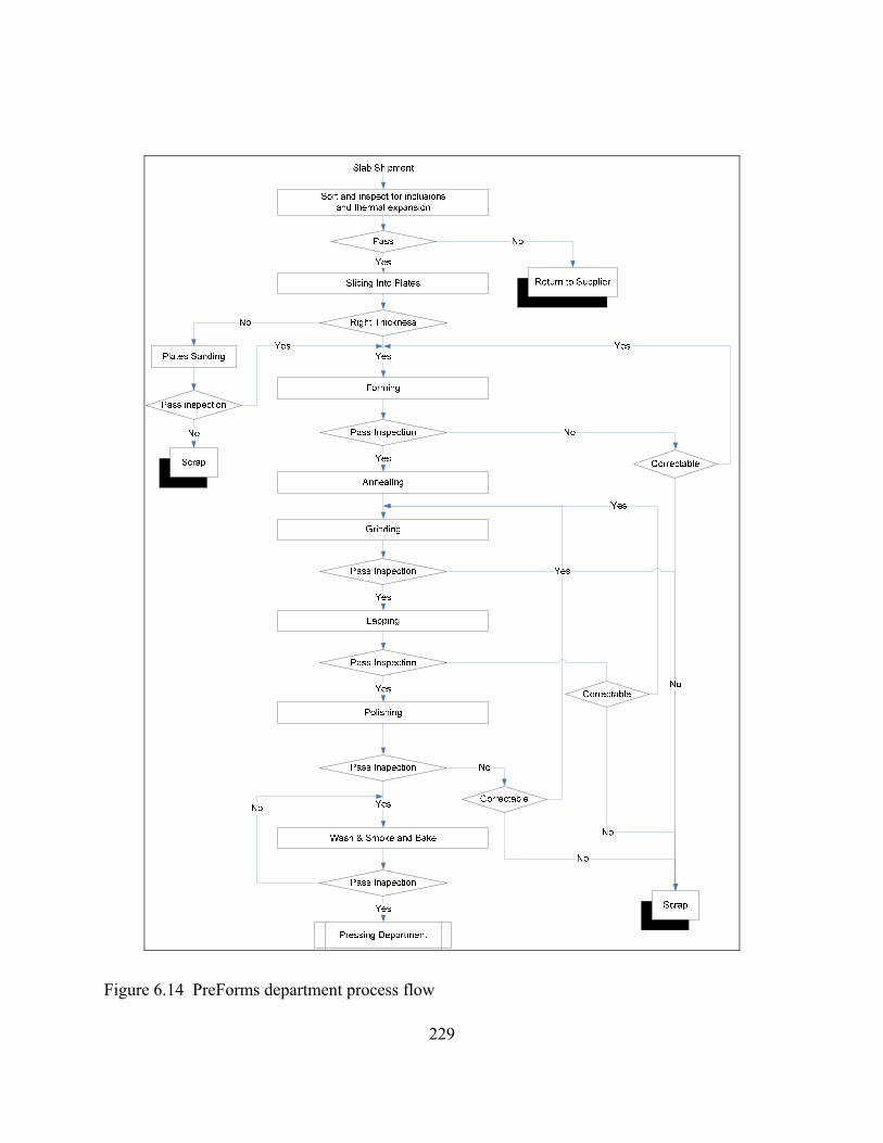
229
Figure 6.14 PreForms department process flow

230
Figure 6.15 Presses department process flow
6.1.5 Defining the SDDES modules
Modularizing starts with defining the sets of inputs and outputs of each module. The
synchronization settings are then defined and the modules are expressed in terms of the SDDES
formalism. First the SDDES modules are defined and formalized in the following sections. Table
6-2 lists the abbreviations for the variables mentioned in the modularization process in this
section. The supplier module is mentioned but not modeled.

231
Table 6.2 Abbreviations of module titles and variables
Modules:
Module Abbreviation Definition
1 Assets ASST The SD assets management module 2 Labor LAB The SD labor management module 3 Liabilities LIAB The SD liabilities management modules 4 Materials Inventory and Ordering MIO The SD raw materials management module 5 PreForms PREF The DES Preforms Department module 6 Pressses PRES The DES Presses Department module 7 Production Planning and Work in
Process PWS The SD production planning , work in process, product
inventory and shipping module 8 Supplier SUP The SD raw materials supplier module
Variables:
Variable Abbreviation Use and Location
1 Annealing Load.Queue ANLQ Annealing process queue Preforms department - PREF 2 Assemble For Slicing.Queue ASLQ Slicing process queue in Preforms department - PREF 3 Batch For Grinding.Queue BGRQ Grinding process queue Preforms department - PREF 4 Batch For Lapping.Queue BLPQ Lapping process queue in Preforms department - PREF 5 Batch For Polishing.Queue BPLQ Polishing process queue in Preforms department - PREF 6 Batch For Smoke and Bake.Queue BSBQ Smoke and bake process in Preforms department -
PREF 7 Batch For Washing.Queue BWSQ Washing process in Preforms department - PREF 8 Batch To Cool Off.Queue BCOQ Cooling off process in Preforms department - PREF 9 Cost of Labor Turnover LTO Total cost of labor turnover - LIAB 10 Cost of Parts Arrival Rate CPAR Contributes to estimating the dollar value of inventory -
ASST 11 Days Supply of Parts Inventory DSPI Available supply of materials considering scheduled
production rate - MIO 12 Desired Labor DL Needed number of workers considering labor
productivity and scheduled production - LAB 13 Dollar Value of Inventory DVI Total value of all inventories – ASST 14 Dollar Value of Sales DVS The inflow rate to the accounts receivable stock – ASST 15 Effect of Cash Constraints on
Hiring ECCH The financial limit on hiring new labor - ASST
16 Effect of Cash Constraints on Parts Ordering
ECCPO The financial limits on ordering materials - ASST
17 Effect of Supplier Capacity on Parts Ordering
ESCPO Constraint of supplier capability on ordering - MIO
18 Finished Goods Inventory FGI Level of finished product units – PWS 19 Hold For Air.Queue HAQ Air pressing section queue in Presses department -
PRES

232
Variable Abbreviation Use and Location
20 Hold For NI.Queue HNIQ Nitrogen pressing section queue in Presses department - PRES
21 Indicated Overtime IOT Estimated overtime needed considering scheduling production and current regular capacity - LAB
22 Indicated Parts Order Rate IPOR Estimated materials ordering considering inventory adjustments and scheduled production - MIO
23 Initial WIP Preforms IWIPF Starting value of the work-in-process at the Preforms processes - PWS
24 Initial WIP Presses IWIPS Starting value of the work-in-process at the Presses processes - PWS
25 Interferometer Tests 35.Queue IT35Q Interferometer testing unit queue for type 35 product in Presses - PRES
26 Interferometer Tests 37.Queue IT37Q Interferometer testing unit queue for type 37 product in Presses - PRES
27 Inspection 35.Queue 35INSQ Inspection for type 35 product queue – PRES 28 Inspection 37.Queue 37INSQ Inspection for type 37 product queue – PRES
29 Issued Preforms IPREF Output of the Preforms department in the form of semi-finished lenses - PREF
30 Labor LBR Labor stock level - LAB 31 Labor Costs LCT Total cost of current labor level - LIAB 32 Labor Firing Rate LFR Rate of firing of current workers - LAB 33 Labor Hiring Rate LHR Rate of joining the current labor - LAB 34 Labor Recruiting Rate LRR Rate of opening new labor positions – LAB 35 Maximum Capacity MXC Limit of regular plus overtime capacity - LAB 36 Molds For Oven.Queue MOQ Prefom oven process queue in Preforms department -
PREF 37 Overtime Preforms OTPF The required level of overtime at Preforms - LAB 38 Overtime Presses OTPS The required level of overtime at Presses - LAB 39 Parts Arrival Rare PAR Inflow rate of materials into materials inventory - MIO 40 Parts Inventory PI Raw materials inventory stock level – MIO 41 Parts Inventory Goal PIG Desirable level of raw materials inventory for smooth
production – MIO 42 Parts On Order POO Level of raw materials in the supply line – MIO 43 Parts On Order Goal POOG Desirable level of raw materials in the supply line
considering supply performance and usage rate – MIO 44 Parts Order Rate POR Rate of ordering raw materials from the supplier – MIO 45 Potential Production from Labor PPL Current capacity considered scheduled overtime - LAB 46 47 Preforms Overtime PFOT Scale factor to set overtime in Preforms - PREF 48 Presses Overtime PSOT Scale factor to set overtime in Presses - PREF 49 Shipment Size SHSZ Amount of materials released into Preforms – PREF 50 Preforms Production Rate PFPR Estimated production rate at the Preforms Department –
PREF

233
Variable Abbreviation Use and Location
51 Preforms Scrap Rate PFSC Estimated scrap rate at the Preforms Department - PREF
52 Preforms WIP PFWIP Estimated level of work-in-process at the Preforms Department - PREF
53 Presses Production Rate PSPR Estimated production rate at the Presses Department – PRES
54 Presses Scrap Rate PSSC Estimated scrap rate at the Presses Department – PREF 55 Presses WIP PSWIP Estimated level of work-in-process at the Presses
Department - PRES 56 Production Completion Rate PCR Rate of finalizing end product, map to Presses
Production Rate - PWS 57 Production Start Rate PSR Rate of starting processing raw materials – PWS 58 Scheduled Production Rate SPR Decided production rate considering demand and
capacity – PWS 59 Shipment Size SHSZ Amount of materials released into Preforms – PREF 60 Shipping Rate SHR Rate of shipping products to customers - PWS 61 Supplier Capacity SC Capacity of materials supplier to meet orders - SUP 62 Supplier Delivery Delay SDD Delay before ordered materials are received - SUP 63 Supplier Demand Rate SDR Customer ordering at the supplier end - SUP 64 Value Added in Process VAP Average cost share in the product unit - ASST 65 WIP Goal Preforms WPGF Estimated desired level of Preforms WIP - PWS 66 WIP Goal Presses WPGS Estimated desired level of Presses WIP - PWS 67 WIP Inventory WIP Total level of work-in-process inventory – PWS 68 Yield YLD Output production as percentage of released materials -
PWS 69 Arriving Preformes Shipment APS Arriving materials at Presses - PRES
6.1.5.1 The MIO module
The function of the MIO is managing the raw materials inventory and the materials
ordering rate. A simplified version of the module is shown in Figure 6-16. The Production Start
Rate on the figure is in fact an input from the PWS module. The rate is shown here for clarity.
The MIO consists of the Parts Inventory stock, which is the main stock to regulate and the Parts
On Order stock, which is the supply line for Parts Inventory. Materials are ordered at the Parts

234
Order Rate, arrive at the Parts Arrival Rate, and they are used at the Production Start Rate. To
maintain the required materials inventory for smooth production, the Indicated Parts Order Rate
includes the Parts Inventory and Parts On Order Corrections to keep the stock levels at the
desired values. Material ordering is planned based on the Scheduled Production Rate from the
PWS module. The Production Start Rate is an input from the PWS module and is determined by
the usage of materials in PWS in addition to the needed adjustments to the stocks in that module.
Financial constraints should also be considered in ordering materials. Besides, the supplier
performance in terms of capacity and delivery delay is necessary to estimate the materials arrival
rate and the limit on the order rate.
Figure 6.16 Simplified view of the SD MIO module
In the SDDES formalism format, the MIO module is specified as given below.
Parts On Order Parts InventoryParts Order Rate Parts Arrival Rate Production Start Rate
+
+
Parts InventoryCorrection
Parts on OrderCorrection
PartsInventory
Goal
Parts OnOrder Goal
Time to adjustParts Inventory
Indicated PartsOrder Rate

235
),,,,( CONTPYXSDMIO MIOMIOMIO=
The sets of inputs and outputs of MIO, referred to MIOX and MIOY respectively are
presented in Table 6-3. MIO interacts with SD modules only and no format or timing
requirements necessary.
Table 6.3 Inputs and outputs of the MIO
MIOX
m vi sm msop mU
ip u t f MIO SPR PWS OP_PWS_01 IP_MIO_01 DSPI CONT NONE IPOR CONT NONE PIG CONT NONE POOG CONT NONE MIO PSR PWS OP_PWS_02 IP_MIO_02 PI CONT NONE MIO SDD SUP OP_SUP_01 IP_MIO_03 PAR CONT NONE POOG CONT NONE MIO SC SUP OP_SUP_02 IP_MIO_04 ESCPO CONT NONE MIO ECCPO ASST OP_ASST_01 IP_MIO_05 IPOR CONT NONE
MIOY
m op vo
YmD
dm mdV
mdip vu t f MIO OP_MIO_01 PI PWS IP_PWS_01 PSR CONT NONE ASST IP_ASST_01 DVI CONT NONE
MIO OP_MIO_02 POR SUP IP_SUP_01 SDR CONT NONE MIO OP_MIO_03 PAR LIAB IP_LIAB_01 CPAR CONT NONE

236
6.1.5.2 The PWS module
The PWS module represents the conversion of raw materials into work-in-process (WIP),
and work-in-process into finished products. A simplified version of the module is shown in
Figure 6-17. There are two work-in-process stocks to correspond to the PreForms and Presses
departments at the shop floor level. Customer order is located in this module and is assumed
fixed; consistent with PMOC that has fairly fixed customer base and demand. Customer order
rate is 25,000 units/month, which is the average monthly demand at PMO Inc. As shown in
Figure 6-17, the Scheduled Production Rate accounts for the demand and the corrections to the
inventory stocks. Production Start Rate is determined accordingly and based on the available raw
materials inventory from MIO and on the available capacity (regular and overtime) from the
Labor module.
PWS also interacts with the PreForms and Presses. Preforms provides accurate estimates
for the Preforms Production Rate, Preforms work in process (WIP), and Preforms Scrap Rate.
Likewise, Production Completion Rate, Presses WIP, and Presses Scrap Rate can be imported
from the Presses module. The DES modules need to import the initial level of WIP from the
PWS so they start at the steady state and consistent with the SD modules configuration. Several
locations in the PreForms and Presses use the initial WIP stock levels form PWS. The DES
modules then update The WIP levels as production proceeds. Production rates and scrap rates are
also provided by the DES modules.

237
Figure 6.17 Simplified version of the SD PWS module
Based on the above description of the interactions between PWS and the other SD and
DES modules, the inputs and outputs of PWS are defined in Table 6-4 in accordance with the
SDDES formalism. The SDDES formalism representation of the PWS module is given below.
),,,,( CONTPYXSDPWS PWSPWSPWS=
PWS interacts with SD and two DES modules. Exchanging data between PWS and each
of PREF and PRES is carried out at the end of each DES segment. In Table 6-4, it is indicated
that data from or to DES and/or SD modules are imported and exported via the SDDES
controller at the end of each DES run segment. The TB_END and TB_START values for the
data exchange timing indicate that data is needed at the start or end of the run segment.
Formatting specifications for the exchanged variables in Table 6-4 are explained below:
PREFORMS WIP PRESSES WIPProduction Start
RatePREFORMS
Production Rate
Presses WIPCorrection
Preforms WIPCorrection
Presses WIPGoal
Preforms WIPGoal
Time to adjustPreforms WIP
Customer OrdrRate
ScheduledProduction Rate
Finished GoodsInventoryProduction
Completion RateShipping Rate
PreformsScrap Rate Presses
Scrap Rate
Time to AdjustPresses WIP
Finished GoodsInventory Goal
Time to AdjustFinished Goods
Inventory
Finished GoodsInfentory
Correction

238
Table 6.4 Inputs and outputs of the PWS
PWSX
m vi sm msop mU
ip u t f PWS PI MIO OP_MIO_01 IP_PWS_01 PSR CONT NONE PWS PPL LAB OP_LAB_01 IP_PWS_02 SPR CONT NONE PWS MXC LAB OP_LAB_02 IP_PWS_03 PSR CONT NONE PWS PFPR PREF OP_PREF_01 IP_PWS_04 PFPR TB_END OBSERVATIONAL_DES_TB >>
TB_BASE_TIME_RATE PWS PFSC PREF OP_PREF_02 IP_PWS_05 YLD TB_END OBSERVATIONAL_DES_TB >>
TB_BASE_TIME_RATE PWS PFWIP PREF OP_PREF_03 IP_PWS_06 WIP TB_END TIME_PERSIST_DES_TB >> TB_END_READ PWS PSPR PRES OP_PRES_01 IP_PWS_07 PCR TB_END OBSERVATIONAL_DES_TB >>
TB_BASE_TIME_RATE PWS PFSC PRES OP_PRES_02 IP_PWS_08 YLD TB_END OBSERVATIONAL_DES_TB >>
TB_BASE_TIME_RATE PWS PFWIP PRES OP_PRES_03 IP_PWS_09 WIP TB_END TIME_PERSIST_DES_TB >> TB_END_READ
PWSY
m op vo
YmD
dm mdV
mdip vu t f PWS OP_PWS_01 SPR MIO IP_MIO_01 DSPI CONT NONE IP_MIO_01 IPOR CONT NONE IP_MIO_01 PIG CONT NONE IP_MIO_01 POOG CONT NONE LAB IP_LAB_01 DL CONT NONE IP_LAB_01 IOT CONT NONE
PWS OP_PWS_02 PSR MIO IP_MIO_02 PI CONT NONE PREF IP_PREF_02 SHSZ TB_START FLOW_SD >> SCALE_TO_DES_EQUIV_RATE PWS OP_PWS_03 IWIPF PREF IP_PREF_01 ANLQ STARTUP STOCK_SD >> SCALE_TO_DES_USER IP_PREF_01 ASLQ STARTUP STOCK_SD >> SCALE_TO_DES_USER

239
PWSY
m op vo
YmD
dm mdV
mdip vu t f IP_PREF_01 BGRQ STARTUP STOCK_SD >> SCALE_TO_DES_USER IP_PREF_01 BLPQ STARTUP STOCK_SD >> SCALE_TO_DES_USER IP_PREF_01 BPLQ STARTUP STOCK_SD >> SCALE_TO_DES_USER IP_PREF_01 BSBQ STARTUP STOCK_SD >> SCALE_TO_DES_USER IP_PREF_01 BWSQ STARTUP STOCK_SD >> SCALE_TO_DES_USER IP_PREF_01 MOQ STARTUP STOCK_SD >> SCALE_TO_DES_USER IP_PREF_01 BCOQ STARTUP STOCK_SD >> SCALE_TO_DES_USER PWS OP_PWS_04 IWIPS PRES IP_PRES_01 HAQ STARTUP STOCK_SD >> SCALE_TO_DES_USER IP_PRES_01 HNIQ STARTUP STOCK_SD >> SCALE_TO_DES_USER IP_PRES_01 IT35Q STARTUP STOCK_SD >> SCALE_TO_DES_USER IP_PRES_01 IT37Q STARTUP STOCK_SD >> SCALE_TO_DES_USER IP_PRES_01 35INSQ STARTUP STOCK_SD >> SCALE_TO_DES_USER IP_PRES_01 37INSQ STARTUP STOCK_SD >> SCALE_TO_DES_USER PWS OP_PWS_05 WIP ASST IP_ASST_02 DVI CONT NONE PWS OP_PWS_06 FGI ASST IP_ASST_03 DVI CONT NONE PWS OP_PWS_07 SR ASST IP_ASST_04 DVS CONT NONE
• OBSERVATIONAL_DES_TB >> TB_BASE_TIME_RATE: Input is DES observational random variable, collected over
TB. Map to SD flow rate given TB
• TIME_PERSIST_DES_TB >> TB_END_READ: Input is DES time-persistent random variable. Use at TB end.
• FLOW_SD >> SCALE_TO_DES_EQUIV_RATE: Input is SD flow rate. Adjust to TB as entities arrival at Destination.
• STOCK_SD >> START_UP_READ: Input is SD stock level. Read at run startup.

240
6.1.5.3 The LAB Module
The LAB module represents the labor management function. As shown in Figure 6-18,
the current level of workforce (Labor stock) is the main stock being regulated. It is increased by
the Labor Hiring Rate and decreased by the firing (if used) and voluntary attrition. Management
estimates the needed correction to labor level based on the active attrition rates considering the
desired labor level, which is decided based on inputs from the production management and
financial units. Management seek to hire new labor at the labor recruiting rate. Labor in the
process of training and completing paper work are represented by the Labor being Recruited
stock. Corrections to the Labor and Labor Being Recruited provide the estimates for the
indicated hiring rate, which is also restricted by the financial constraints. At this module also and
based on the scheduled production, the level of overtime is estimated to meet the schedule.
Available capacity (regular and overtime) is the limit over the production rate at the PWS
module.
The LAB module interacts with the PWS and Liabilities modules. It uses the scheduled
production rate from PWS to estimate the needed overtime and desired labor level and sets the
limits over the feasible production rate at the PWS. Hiring and attrition are restricted by the
financial constraints. The current labor level is an input to the liabilities module to estimate the
cost of labor turn over and production expenses. Table 6-5 presents the sets of inputs and outputs
for the LAB module along with the rest of its formalism information.

241
Figure 6.18 Simplified version of the SD LAB module
The LAB model is expressed in terms of the SDDES formalism as follows.
),,,,( CONTPYXSDLAB LABLABLAB=
Labor BeingRecruited Labor
LaborRecruiting
Rate
Labor Hiring Rate Labor AttritionRate
+
+
Correction tolabor
Correction to laborbeing recruited
Desired Labor
Desired laborbeing recruited
Indicatedhiring rate
LaborFiringRate

242
Table 6.5 Inputs and outputs of the SD LAB module
MIOX
m vi sm msop mU
ip u t f LAB SPR PWS OP_PWS_01 IP_LAB_01 DL CONT NONE IOT CONT NONE
LAB ECCH ASST OP_ASST_01 IP_LAB_02 LRR CONT NONE
MIOY
m op vo
YmD
dm mdV
mdip vu t f LAB OP_LAB_01 PPL PWS IP_PWS_02 SPR CONT NONE LAB OP_LAB_02 MXC PWS IP_PWS_03 PSR CONT NONE LAB OP_LAB_03 LBR LIAB IP_LIAB_02 LCT CONT NONE VAP CONT NONE
LAB OP_LAB_04 LHR LIAB IP_LIAB_03 CLT CONT NONE LAB OP_LAB_05 LFR LIAB IP_LIAB_04 CLT CONT NONE LAB OP_LAB_06 OTPF PREF IP_PREF_03 PFOT TB_START NONE LAB OP_LAB_07 OTPS PRES IP_PRES_03 PSOT TB_START NONE
6.1.5.4 The PREF module
The PREF module interacts with the PWS module and the PRES module. PREF is
driven by the production start rate from PWS. Production start rate (is the estimated rate at which
raw materials start processing. It represents the implementation of the scheduled production.
PREF also receives the level of overtime from the Labor module, should overtime be needed.
The feedback from PREF is its production rate, its scrap rate, level of work in process, and
process cycle time. This feedback information from PREF is collected at the end of the run
segment. Updated values of production start rate and overtime are calculated by PWS based on
that. The production start rate is converted into arrival rate of materials at PREF. Overtime needs

243
no formatting. Production rate and scrap rate from PREF are observational data (number of units
that finished processing and number of units that were scrapped during the run segment) and
they are converted into equivalent rate quantities over the run segment duration and then scaled
to the SD base time unit before they can be used in PWS.
PREF module is the source of materials for PRES. Semi finished lenses (the preforms)
from PREF are the materials for PRES. Preforms, observation data in PREF, are issued daily to
PRES. No formatting is needed to use the PREF production in PRES. PREF module is expressed
as a SDDES module as follows:
),,,,( TBPYXDESPREF PREFPREFPREF=
The sets of inputs and outputs of PREF are given in Table 16-5. The TB_END and
TB_START values for the data exchange timing indicate data needed at start or end of the run
segment. Formatting specifications are explained below.
• STOCK_SD >> SCALE_TO_DES_USER: Input variable is based on an SD stock variable
and should be scaled to initialize the DES user variable.
• FLOW_SD >> SCALE_TO_DES_EQUIV_RATE: Input variable is based on an SD flow
rate variable and should be scaled to TB as DES entities creation rate.
• OBSERVATIONAL_DES_TB >> TB_BASE_TIME_RATE: Input variable is based on
observational data from DES module that was collected over the TB duration. This
data should be converted into a rate variable over TB to be usable in the SD module.
• TIME_PERSIST_DES_TB >> TB_END_READ: Input variable is based on time-persistent
data from DES module. The TB-end value is usable in the SD module.
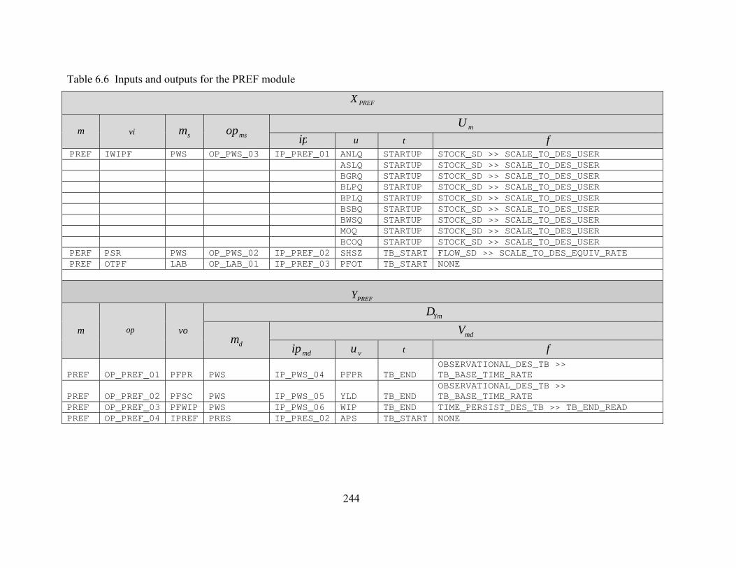
244
Table 6.6 Inputs and outputs for the PREF module
PREFX
m vi sm msop mU
ip u t f PREF IWIPF PWS OP_PWS_03 IP_PREF_01 ANLQ STARTUP STOCK_SD >> SCALE_TO_DES_USER ASLQ STARTUP STOCK_SD >> SCALE_TO_DES_USER BGRQ STARTUP STOCK_SD >> SCALE_TO_DES_USER BLPQ STARTUP STOCK_SD >> SCALE_TO_DES_USER BPLQ STARTUP STOCK_SD >> SCALE_TO_DES_USER BSBQ STARTUP STOCK_SD >> SCALE_TO_DES_USER BWSQ STARTUP STOCK_SD >> SCALE_TO_DES_USER MOQ STARTUP STOCK_SD >> SCALE_TO_DES_USER BCOQ STARTUP STOCK_SD >> SCALE_TO_DES_USER
PERF PSR PWS OP_PWS_02 IP_PREF_02 SHSZ TB_START FLOW_SD >> SCALE_TO_DES_EQUIV_RATE PREF OTPF LAB OP_LAB_01 IP_PREF_03 PFOT TB_START NONE
PREFY
m op vo
YmD
dm mdV
mdip vu t f
PREF OP_PREF_01 PFPR PWS IP_PWS_04 PFPR TB_END OBSERVATIONAL_DES_TB >> TB_BASE_TIME_RATE
PREF OP_PREF_02 PFSC PWS IP_PWS_05 YLD TB_END OBSERVATIONAL_DES_TB >> TB_BASE_TIME_RATE
PREF OP_PREF_03 PFWIP PWS IP_PWS_06 WIP TB_END TIME_PERSIST_DES_TB >> TB_END_READ PREF OP_PREF_04 IPREF PRES IP_PRES_02 APS TB_START NONE

245
6.1.5.5 The PRES module
The PREF interacts with the PREF module to get raw materials. It also needs to be
initialized at the start of the SDDES simulation run. Initialization involves initial work in process
level from the PWS module. It also uses the overtime information from the LAB module. Its
outputs are its production rate, scrap rate, level of work in process, cycle time. These outputs are
exported to the PWS module. The PRES module is described in SDDES formalism format as
given below.
),,,,( TBPYXDESPRES PRESPRESPRES=
The sets of inputs and outputs are listed in Table 6-6. The TB_END and TB_START
values for the data exchange timing indicate that data is needed at start or end of the run
segment. Formatting specifications are explained below.
• STOCK_SD >> SCALE_TO_DES_USER: Input variable is based on an SD stock variable
and should be scaled to initialize the DES user variable.
• OBSERVATIONAL_DES_TB >> TB_BASE_TIME_RATE: Input variable is based on
observational data from DES module that was collected over the TB duration. This
data should be converted into a rate variable over TB to be usable in the SD module.
• TIME_PERSIST_DES_TB >> TB_END_READ: Input variable is based on time-persistent
data from DES module. The TB-end value is usable in the SD module.
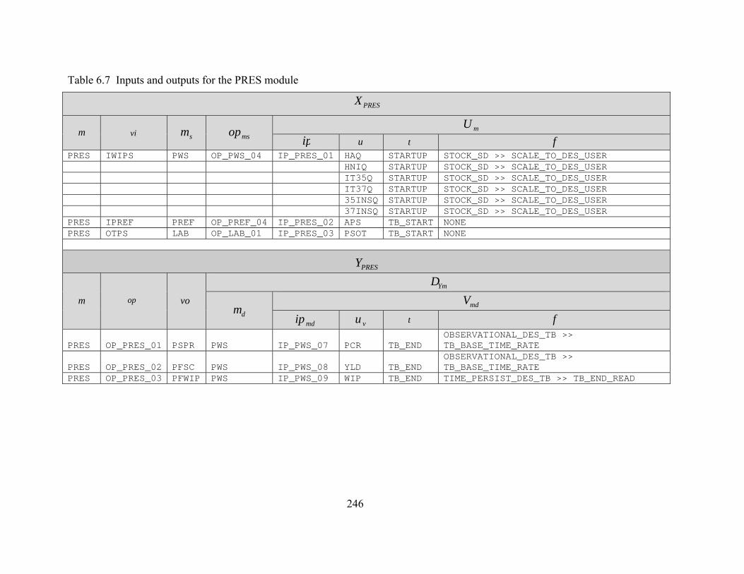
246
Table 6.7 Inputs and outputs for the PRES module
PRESX
m vi sm msop mU
ip u t f PRES IWIPS PWS OP_PWS_04 IP_PRES_01 HAQ STARTUP STOCK_SD >> SCALE_TO_DES_USER HNIQ STARTUP STOCK_SD >> SCALE_TO_DES_USER IT35Q STARTUP STOCK_SD >> SCALE_TO_DES_USER IT37Q STARTUP STOCK_SD >> SCALE_TO_DES_USER 35INSQ STARTUP STOCK_SD >> SCALE_TO_DES_USER 37INSQ STARTUP STOCK_SD >> SCALE_TO_DES_USER PRES IPREF PREF OP_PREF_04 IP_PRES_02 APS TB_START NONE PRES OTPS LAB OP_LAB_01 IP_PRES_03 PSOT TB_START NONE
PRESY
m op vo
YmD
dm mdV
mdip vu t f
PRES OP_PRES_01 PSPR PWS IP_PWS_07 PCR TB_END OBSERVATIONAL_DES_TB >> TB_BASE_TIME_RATE
PRES OP_PRES_02 PFSC PWS IP_PWS_08 YLD TB_END OBSERVATIONAL_DES_TB >> TB_BASE_TIME_RATE
PRES OP_PRES_03 PFWIP PWS IP_PWS_09 WIP TB_END TIME_PERSIST_DES_TB >> TB_END_READ

247
6.1.6 DES modules run segmentation and resumption
The implementation of the resumption algorithm provided very good approximation to
maintain the state of the DES modules between the segments. Production rate at the Presses
department at PMOC is scheduled weekly for the daily production size. Press operators retrieve
materials from the PreForms department at the beginning of each work day for the stated
production of the day. Schedule is revised based on the performance. The PREF and PRES
modules were thus configured to run for one-day segments to represent the actual work practices.
Each one-day segment is a complete DES run. The output from each PRES segment at day k is
the input to the PRES segment at day k+1.
We tested the segmented DES modules in comparison to the original non-segment
modules for both PREF and PRES. The PREF module was run for a period of two months
without segmentation and was then run after implementing the resumption algorithm and
segmenting its run into one-day segments. In both cases the module received fixed production
start rate value from PWS to create the raw materials. Daily production rate, scrap, and WIP
were observed in the two cases. The two data samples (large sample size of 50) generated by the
two module versions were tested for the difference between the means. The null hypothesis was
that the two sample means are equal. Variances were not assumed equal. The test results showed
no sufficient evidences (at 95% confidence level) to suggest that the observed measures were
different when using segmented DES module from their values when using the original non-
248
segmented DES model. Similar statistical testes were done for the PRES modules. Appendix B
presents the test results for the two modules.
6.1.7 SDDES model validation
The SDDES model was validated at the face validity and data validity levels. The SD and
DES modules were tested for face validity in a cyclic model review process with the production
managers of the PreForms and Presses departments and with the senior managers who
participated in the development of the SD modules. The DES modules were also reviewed with
the operators at the two departments as some data assumptions (processing times, batch sizes,
loading/unloading times, and rejection rates at the PreForms department in particular) were made
based on their inputs. The objective of the face validity process was to confirm that the modules
satisfactorily captured the system structure for the units they modeled and represent their actual
behaviors. Face validity establishes the starting level of confidence in the SDDES model and
points out the areas needing enhancement or corrections. Yet face validity is not sufficient to
consider the model valid. The model validity decision is made based on data validation by
comparing its output data to the actual system data using statistical techniques.
Data validation was performed at the module level and at the whole SDDES model level.
It involved statistical comparisons of the model-generated data and the system data. The primary
measures of performance were the production and scrap rates and the level of work-in-process.
Data generated by the SDDES model were used for testing. Using a large sample size (50) and

249
making no assumption about the variances of the SDDES model or system data, the two sample
t-test of the difference between means was utilized. Table 6-7 and 6-8 show the test results for
the difference between mean production rates for the PreForms and Presses departments
respectively. Table 6-9 and 6-10 show the test results for the scrap rates of the system and model
at the two departments. The test results show no sufficient evidences to suggest that the model
generated data is different from the actual system data. Based on the statistical tests, the SDDES
was considered valid. The interfaced DES and SD modules could model and reflect the actual
system behavior of PMOC as approved by the system experts and according to the statistical
tests.

250
Table 6.8 Testing the difference between the preforms mean production rates – system data vs. SDDES model data Two-sample T for System vs Model N Mean StDev SE Mean System 50 1791 201 28 Model 50 1806 301 43 Difference = mu System - mu Model Estimate for difference: -15.7 95% CI for difference: (-117.6, 86.2) T-Test of difference = 0 (vs not =): T-Value = -0.31 P-Value = 0.760 DF = 85
System Model
1000
1500
2000
2500
Boxplots of System and Model(means are indicated by solid circles)
System Model
1400
1900
2400
Dotplots of System and Model(means are indicated by lines)

251
Table 6.9 Testing the difference between presses mean production rates – system data vs. SDDES model data Two-sample T for System vs Model N Mean StDev SE Mean System 50 1251.5 61.7 8.7 Model 50 1247.9 67.4 9.5 Difference = mu System - mu Model Estimate for difference: 3.6 95% CI for difference: (-22.0, 29.3) T-Test of difference = 0 (vs not =): T-Value = 0.28 P-Value = 0.779 DF = 97
System Model
1000
1100
1200
1300
1400
Boxplots of System and Model(means are indicated by solid circles)
System Model
1000
1100
1200
1300
1400
Dotplots of System and Model(means are indicated by lines)

252
Table 6.10 Testing the difference between PreForms mean scrap rates – system data vs. SDDES model data Two-sample T for System vs Model N Mean StDev SE Mean System 51 195.7 41.8 5.9 Model 51 190.3 52.2 7.3 Difference = mu System - mu Model Estimate for difference: 5.43 95% CI for difference: (-13.17, 24.03) T-Test of difference = 0 (vs not =): T-Value = 0.58 P-Value = 0.563 DF = 95
System Model
100
200
300
400
Boxplots of System and Model(means are indicated by solid circles)
System Model
50
150
250
350
Dotplots of System and Model(means are indicated by lines)

253
Table 6.11 Testing the difference between Presses mean scrap rates – system data vs. SDDES model data -sample T for System vs Model N Mean StDev SE Mean System 51 535.1 57.7 8.1 Model 51 540.7 47.2 6.6 Difference = mu System - mu Model Estimate for difference: -5.6 95% CI for difference: (-26.3, 15.1) T-Test of difference = 0 (vs not =): T-Value = -0.53 P-Value = 0.595 DF = 96
System Model
350
450
550
650
Boxplots of System and Model(means are indicated by solid circles)
System Model
350
450
550
650
Dotplots of System and Model(means are indicated by lines)

254
6.1.8 Synchronizing the SD and DES
The SDDES controller implements the synchronization mechanism (Section 5.5) to
interface the simulation modules as specified by the formalism in Section 6.1.4. In the current
experiment the PWS, LAB, MIO, PREF, and PRES are interfaced. The interactions between the
SD and DES occur between PWS and PREF and PRES. Figure 6-19 represents the overlap
between these three modules. PREF is the left ellipse covering while PRES is the right eclipse.
The two DES modules also interact between themselves and with the LAB module for updated
capacity and overtime usage information. This overlap between these modules is the core of the
experiment conducted in this work as explained later.
Figure 6.19 Overlap between SD and DES in the internal supply chain functions
PREFORMS WIP PRESSES WIPProduction Start
RatePREFORMS
Production Rate
Presses WIPCorrection
Preforms WIPCorrection
Presses WIPGoal
Preforms WIPGoal
Time to adjustPreforms WIP
Customer OrdrRate
ScheduledProduction Rate
Finished GoodsInventoryProduction
Completion RateShipping Rate
PreformsScrap Rate Presses
Scrap Rate
Time to AdjustPresses WIP
Finished GoodsInventory Goal
Time to AdjustFinished Goods
Inventory
Finished GoodsInfentory
Correction

255
Figure 6-20 depicts the variables exchanged between the PREF, PRES modules at the
DES side and the internal supply chain SD modules, as defined by the formalized modules. The
current experiment is focused on demonstrating the interfacing of these modules. These
interactions are implemented by the controller as shown by the synchronization diagram in
Figure 6-21.
Figure 6.20 The exchanged variables between the SD and DES in the current experiment
In Figure 6-21 the SD modules are combined together as SD for clarity whereas the two
DES modules are indicated explicitly. The segment length for the DES modules is set equal to
the SD computational time step for simplicity. The sequence of interactions is executed as
follows:
1. At the simulation model start up (time 0):

256
a. The SDDES controller imports the initialization data from the SD modules
<arrow 1>. This includes the initial work in process (WIP), overtime (OT) for
PREF and PRES use, the initial production start rate (PSR) for PREF use, and
the initial PREF production rate (PR), desired shipping rate (DSR) and yield
for PRES use. The initial values are exported after satisfying any formatting
requirements to PREF and PRES <arrows 2 and 3>.
b. PREF and PRES are signaled to run the first segment <arrows 4 and 5>.
2. At the end of the first segment (time Δt):
a. The SDDES controller collects the WIP, PR and scrap level from PREF and
the WIP, production completion rate (PCR), and scrap level from PRES
<arrows 6 and 7>. These feedback data is exported to the SD modules (PWS)
after satisfying all required formatting <arrow 8>.
b. SD is signaled to advance its time to Δt and perform its first segment
calculations using the DES feedback <arrow 9>.
c. The controller imports the updated PSR, DSR, OT, yield from PWS and LAB
<arrow 10>. The updates inputs are exported to the appropriate DES module
in addition to exporting the PR from PREF to PRES as the raw materials for
the pressing operations <arrows 11 and 12>.
d. The DES modules are signaled to run the second segment to advance to time
2Δt.
3. At the end of the second segment (time 2Δt) and each segment afterward, the

257
transactions a through d in (for arrows 4 through 12) Step 2 above are repeated using
the updated data created by the modules at time nΔt, where n is the number of the
segment just completed by the DES modules.

258
tΔ tΔ2 tnΔ
Figure 6.21 Synchronization sequence in executing PMOC's SDDES model

259
6.1.9 Results and Discussion
The objective of the current experiment is demonstrating the potential of SDDES to
model the manufacturing system. The modules were synchronized as described in the previous
section to exchange the inputs and outputs specified in the SDDES formalism at the specified
format and timing. We ran the model for a period of three months without external stimulation.
The current customer order rate was kept fixed to allow observing the effect of exchanging the
data between the DES and SD modules. Starting at equilibrium at time zero, the desired
production rate of the final product; represented by the desired shipping rate is estimated at the
PWS module based on the known customer order rate. PWS also estimates the appropriate
material usage rate (production start rate) given the available raw materials inventory level and
production capacity. Desired shipping and production start rate are exported to the PRES and
PREF modules respectively. The PREF module uses the production start rate to produce raw
preforms which the PRES module uses to meet the desired shipping rate. The outputs of PREF
and PRES are exported to the PWS so it can update its estimates of the desired shipping and
usage rates.
Figure 6-22 and 6-23 show the production rates at the PREF and PRES respectively. It is
observed that the two modules perform at a horizontal trend as the customer order rate is fixed.
As can be seen the productivity at PRES follows the productivity at PREF. the output of PREF is
the input to PRES. A drop in PREF’s production before the end of week 1, at week 5, and after
week 10 causes corresponding drops in PRES’ productivity at the following work days.

260
Figure 6.22 PreForms production rate by SDDES
Figure 6.23 Presses production rate by SDDES
Preforms Production Rate20,000
15,000
10,000
5,000
00 1 2 3 4 5 6 7 8 9 10 11 12
Time (week)
Preforms Production Rate : SDDES units/week
Presses Production Rate20,000
15,000
10,000
5,000
00 1 2 3 4 5 6 7 8 9 10 11 12
Time (week)
Presses Production Rate : SDDES units/week

261
Since PRES is controlled by the desired shipping rate from PWS, its productivity tends to
show less variability compared to PREF. PRES uses the necessary amount of raw preforms from
PREF to match the desired shipping rate while PREF is managed to use all raw materials
available to it given that raw materials have been ordered to meet the customer order rate.
PREF and PRES productivity is exported to PWS along with their scrap and WIP
performances (Figure 6-24 through 6-27). When made available at PWS, the module updates its
estimates of the production start rate, desired shipping rate, and the scheduled production rate.
The SD module also updates the finished goods inventory level and ships to meet the current
customer orders. If production from PRES is below expected level, the unmet customer orders
are added to the desired shipping rate so that PRES is instructed by PWS fulfill them at the
following work days. Raw materials to meet the unmet orders are ordered based on the deviation
in the finished goods inventory level from its desired level.
It should be noted that any value generated by a module being; a DES or an SD is in fact
an SDDES-generated value. In SDDES the interfaced modules are not independent of each other.
They are all components of the same simulation model acting as parts of a set of overlapping
feedback loops. Although the PREF production rate, for instance, is generated by PREF it is
exported to PRES and PWS. New estimates from PWS are made based on it to be the inputs to
PREF. Thus the following production rate from PREF is actually a function of PREF current
configuration and the inputs obtained from PWS that are in turn functions of the PRES data and
the other SD modules as well.

262
Figure 6.24 PreForms scrap rate by SDDES
Figure 6.25 PreForms work in process level by SDDES
Preforms Scrap Rate2,500
1,875
1,250
625
00 1 2 3 4 5 6 7 8 9 10 11 12
Time (week)
Preforms Scrap Rate : SDDES units/week
PreForms Work In Process Level15,000
12,500
10,000
7,500
5,0000 1 2 3 4 5 6 7 8 9 10 11 12
Time (week)
Preforms WIP Level : SDDES units

263
Figure 6.26 Presses scrap rate by SDDES
Figure 6.27 Presses work in process level by SDDES
Presses Scrap Rate5,000
3,750
2,500
1,250
00 1 2 3 4 5 6 7 8 9 10 11 12
Time (week)
Presses Scrap Rate : SDDES units/week
Presses Work In Process Level5,000
3,750
2,500
1,250
00 1 2 3 4 5 6 7 8 9 10 11 12
Time (week)
Presses WIP Level : SDDES

264
Given the PRES production rate, PWS monitors the finished goods inventory level and
consequently the unshipped demand, which is the demand that could not be met so far due to
unexpected drops in PRES productivity. Figure 6-28 shows the finished goods inventory level at
PWS. Comparing this inventory level to PRES production rate (Figure 6-24) shows that the drop
in production at PRES at weeks 1 and 5 and after week 10 corresponds to the starting of finished
inventory level to decrease.
The drop in finished goods inventory below the current customer order rate increases the
unshipped demand as shown in Figure 6-28. PWS estimates the unshipped and updates the
desired shipping rate to account for the unshipped quantities. At equilibrium, the desired
shipping rate (Figure 6-28) should equal the customer order rate but it increases as the unshipped
increases, following the level of the finished product inventory. The updated desired shipping
rate is exported to PRES such that it pulls more raw preforms (if available) from PREF to
produce to meet both current customer order rate and the delayed demand (the unshipped).
Experiencing delayed customer order rate leads to the occasional increase in the delivery
delay. The normal delivery delay quoted by the company is one week. Delayed orders are
shipped as soon as they are available. Due to unavailable production, occasional delays of an
extra one day may occur as shown in Figure 6-28; some orders are shipped the following day
after their due dates.
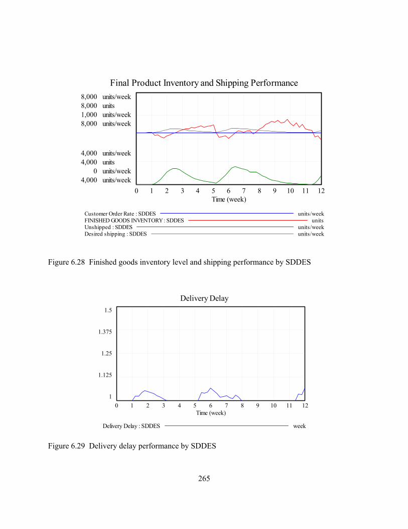
265
Figure 6.28 Finished goods inventory level and shipping performance by SDDES
Figure 6.29 Delivery delay performance by SDDES
Final Product Inventory and Shipping Performance8,000 units/week8,000 units1,000 units/week8,000 units/week
4,000 units/week4,000 units
0 units/week4,000 units/week
0 1 2 3 4 5 6 7 8 9 10 11 12Time (week)
Customer Order Rate : SDDES units/weekFINISHED GOODS INVENTORY : SDDES unitsUnshipped : SDDES units/weekDesired shipping : SDDES units/week
Delivery Delay1.5
1.375
1.25
1.125
10 1 2 3 4 5 6 7 8 9 10 11 12
Time (week)
Delivery Delay : SDDES week

266
The raw materials inventory (Parts Inventory) is estimated by the MIO module based on
the scheduled production rate from PWS that is calculated to accommodate the PREF and PRES
productivity and the shipping performance. Based on the scheduled production rate, MIO orders
the needed raw materials. The production start rate of PWS is a function in the availability of the
raw materials in the Parts Inventory stock and the available production capacity from the LAB
module. The oscillating behavior of the Parts Inventory level (Figure 6.30) is the result of the
behavior of the work-in-process in PREF (Figure 6-25), the work-in-process in PRES (Figure 6-
27), the finished goods inventory level (Figure 6.29), and the changes in the shipping rate (Figure
6-29). The combined behaviors of these variables contribute to the estimating of the scheduled
production rate (Figure 6.30) at PWS that drives the materials ordering and the parts inventory
level in MIO. The time lag between the scheduled production rate and the parts inventory level is
supplier delivery delay period.

267
Figure 6.30 Scheduled production rate and raw materials inventory behaviors by SDDES
6.1.10 Reviewing the SDDES model results with PMOC
It was shown that the SD and DES modules in the PMOC SDDES model are interacting
appropriately and the model could be used to explain the behavior of the system at the shop floor
and planning level. It is concluded that the variation in production rate, particularly at the
PreForms department and at the Presses department are the root cause of the oscillating behavior
(although around a horizontal trend) observed for some of the system variables (inventory levels)
Parts nventory Level and Scheduled Production Rate15,000 units15,000 units/week
10,500 units10,500 units/week
6,000 units6,000 units/week
0 1 2 3 4 5 6 7 8 9 10 11 12Time (week)
PARTS INVENTORY : SDDES unitsScheduled Production Rate : SDDES units/week

268
and shipping performance. Even with a stable level of demand and no special occurrences at the
shop floor, the system occasionally fell short of meeting demand and the inventory levels
oscillated.
We reviewed the model results with the PreForms department’s production manager and
with the manager of operations of the company. With the fixed customer order rate they have
recognized the behavior generated by the model as familiar adding that the variability in the
daily production is due to the large number of product types with relatively small order sizes for
each type. Their commitment to meet loyal customer orders led to the need to manage the
production line in that manner. Synchronization between PreForms and Presses was continuously
in focus but used to be tedious to achieve. The high scrap rate in the Presses would negatively
affect the scheduling and synchronization efforts. Attracting larger order sizes and minimizing
the number of variants of the product types was not an easy decision because of using pressing
technology that was not economically competitive. The metallic molds for the pressing heads at
the Presses department become defective when a pressing attempt fails. Molds would require to
be sent for machining or they would be scrapped as well. Japanese and Korean and other
competitors use ceramic-based pressing heads that had longer service lives and were cheaper. In
addition the company was committed to its long-term customer needs and its higher prices could
not attract more demand. Unwilling to invest in renovating the production facilities at PMO, the
company eventually outsourced the PMO operations in favor of directing their financial
resources to the GRADUIM alloys production and other markets.
As for using the SDDES model, it was perceived as useful tool to improve the

269
communications between the shop floor managers at the level and the operations manager (VP
level). The lack of timely communications and updated data between the operational and
aggregate levels is a real concern. The estimates of the system capacity used to differ from the
production manager and the operations manager (as expressed by the production manager). The
operations manager level uses data from the company’s central database (Spreadsheet based
application) and from other units including engineering, materials, etc. As described by the
PreForms production manager:
• More often than otherwise, the VP team over estimates the system performance; the
reason being the use of data from the centralized database as well as their most recent
knowledge of the system capabilities. The production manager would request permits
for using overtime or extra materials ordering (which are the VP decisions) to match
the expectations.
• Due to significant differences in estimating the system yield (lower yield expected by
VP than what the production manager knew about her production line capabilities !),
they launched a project to evaluate each individual equipment unit’s performance to
update the central database. Need for that was caused by changes at the shop floor
made by the production manager as she started her job that. The data available at the
VP level and in the data base was compiled under a previous production manager and
could not be updated on a timely way.
• The production manager expressed an interest in having a tool that she could
manipulate to reflect the current status (as it frequently changes) so she can be able to

270
communicate accurately to the VP and CEO and avoid the “frustration of convincing
them” of the actual situation in the meetings.
The operations VP considered SDDES valuable to experiment and evaluate the
performance of the system and the impact of the resource allocation (materials, and manpower)
decision on the shipping performance. The causal relationships captured in SDDES can save the
time analyzing and summarizing the collected data at the central database. And he suggested
including the database as an integer component of SDDES to benefit from SDDES in analyzing
the system data.
6.2 Modeling the Manufacturing Value Chain2
The value chain describes the activities performed by organizations and how they lead a
competitive advantage (Porter 1985). The value chain of the manufacturing enterprise can be
viewed as extending the scope of the production/assembly supply chain to include the marketing
and sales and service activities in addition to the supporting activities (Figure 6-31), all when
managed properly at the most cost-effective way improve the generation and sustenance of
growth and lead to a higher competitive position. The value chain partners perform and
coordinate all design, engineering, production, and information flow necessary to manufacture
2 Rabelo et al, (2007). Value chain analysis using hybrid simulation and AHP. Intl J of Production Economics, (105) 536-547

271
products and provide services that meet customers’ needs at the lowest costs. Yet the system
becomes more complex for modeling and analysis.
In the manufacturing value chain where the majority of resources and costs are allocated
to manufacturing and service operations, organizations should concentrate on these areas in order
to maximize savings and consequently the profit margin. This should be approached while
maintain a high degree of vertical integration with the system. From a modeling perspective
hybrid, comprehensive simulation models with the systemic coordinated macro and micro views
are necessary to analyze and manage such complex systems in consistence with strategic
business objectives. This is of particular importance in the global economy of today, where
companies operate across countries’ borders giving significance to the decentralized
organizational structures and the modularization of the business processes.
Figure 6.31 The value chain system
SD with its system view offers an effective framework to model the scope of the value
chain at the aggregate strategic level over long range analysis horizons. Meanwhile, DES models

272
are mainly flow models that track the flow of entities through a system making them appropriate
and effective in building detailed models of the operational level activities (See Table 2-4 in
Chapter 2 for comparing SD and DES). The SDDES hybrid simulation framework can support
the simulation modeling of the value chain of the manufacturing enterprise.
In this section, SDDES is used to build a hybrid simulation model of the value chain
system of a construction equipment manufacturer. Two strategic business units are at the focus
of the analysis: the manufacturing facility (SBU1) and the service providing facility (SBU2). The
analysis of the value chain system helps achieving a competitive advantage in two ways: by
developing a cost advantage through a better understanding of the costs associated with the
value-adding processes and working to minimize them and by differentiation where the focus is
given to enhancing current competencies and capabilities to outperform competitors. In their
effort to achieve a competitive advantage through minimizing costs while maintain quality and
high level of customer satisfaction, the construction equipment manufacturer is considering
outsourcing some, or all of the manufacturing activities. Outsourcing the value chain activities
should be considered if there are the possibilities of getting the activity performed at a lower cost
by a supplier. This also considers the opportunities for improvements in performance (e.g. lead
times, and responsiveness). However, companies should also estimate the risk associated with
outsourcing a value chain activity, which could be considered a core competency, as well as the
risk associated with keeping the activity in-house on the overall system performance. An analysis
of the outsourcing alternatives should be approached from an integrative perspective. The value
chain activities are not isolated from each other. They affect each other in terms of costs and

273
performance.
In the SDDES model of this manufacturing value chain, SD is used to model the entire
value chain system and the strategic decision making processes at the extended enterprise system
while DES is used to provide detailed models of the service and manufacturing sub-systems that
interact directly with the customers. SD provides a comprehensive view of the system allowing
decision makers to analyze the impact of the outsourcing decision on the system as a whole. And
as the main driver to consider outsourcing is cost-effectiveness, accurate estimates of costs
associated with each outsourcing alternative are necessary. In addition the estimate of the
customer satisfaction level will be made based on detailed estimates of the level of
responsiveness and lead times related to delivering products and services. These lend themselves
to the modeling in DES models of the manufacturing and service business units.
The SDDES model is used to assess an outsourcing decision based on the projected
performance over the period of five future years for each outsourcing alternative. The model
works by having SD estimate the demand for the products and the services, the quality of each,
customer reactions to quality of provided service and product, the investment decisions,
overhead costs, and the new product and service development functions. This data are exported
to the DES models of the manufacturing and service units separately to assess the performance
of the manufacturing and service facilities and provide estimates the associated costs. Costs and
number of units produced and services provided are fed back to SD to re-evaluate the overall
performance of the entire system. Figure 6-32 depicts the interactions among the SD and the
DES modules where product and service quality are functions of investments and new products

274
and service designs developed based on the SD model.
Figure 6.32 Data exchanged between SD and DES in the value chain model
The company is evaluating the following three alternatives for outsourcing the
manufacturing facilities:
A. Keep the manufacturing facility (SBU1) and the service facility (SBU2) under the
enterprise and in continental USA
B. Outsource the majority of SBU1 to South East Asia (but to keep the core
competencies of design and new product and service development in house) and keep
SBU 2 in the continental USA
C. Outsource the majority of SBU1 to East Asia (but to keep final manufacturing
performance testing in the continental USA and the core competencies of design, and
new product and service development in house) and keep SBU2 under the
organization.

275
The management wants to base the evaluation of the three alternatives on four factors (1)
profitability, (2) customer satisfaction, (3) responsiveness, and (4) political stability. Profitability
is measured as the net total profits after all costs. In a profitable year, 30% of profits are paid as
taxes, one third after taxes is paid as dividends, and the rest is reinvested to improve
performance. These with the considerations for new product and service development costs and
general administration costs are modeled in SD. The DES models estimate the manufacturing
and service delivery costs. Customer satisfaction (in SD) is measured in several dimensions
based on returns, requests for proposals, service levels, and retention of customers.
Responsiveness is measured as the total replenishment (lead) time needed to satisfy any order
placed. This factor is very important as it significantly contributes to being able to adapt to
variations in the market demand at the customers’ end.
The political stability factor was not part of the simulation models. Decision makers had
to assess it themselves. East Asia is relatively stable and strongly emerging in the international
economy, which offers a trustable business environment. Meanwhile other parts in Southeast
Asia are experiencing a few instabilities due to some military and violent actions, in addition to
relatively less stable governments. In addition, the economic crises that hit Southeast Asia during
the past decade are still in memory. The assessment of relative weight of the four factors was
made using the analytical hierarchy process (AHP) based on the inputs from the SDDES
simulation model for each model.
276
6.2.1 The SD and DES value chain system simulations
The SD model for the value chain model, shown in Figure 6-33, consists of three main
units to represent SBU 1 for the manufacturing facilities and its performance measures, the SBU
2 for the service facilities and its performance measures, the customer management sections for
the customer request for proposals, acquisition, loss, and recovery for demand and customer
retention and satisfaction. Further, the SD model includes the financial environment representing
profits estimates and the investment decisions, productivity and manpower requirements, for
each of the SBU1 and SBU 2. Having a good ratio of service staff to customer means better
customer satisfaction and increased number of customers. Investments in the service
organization imply more investments in staff development and higher service rate. It is important
to invest in service staff but it is critical to keep the balance as good service and higher
satisfaction are dependent on good products. The SD model was validated in Rabelo et al.
(2004). To capture the details of the manufacturing and service facilities, DES models were built
SBU 1 and SBU 2. Generic flow diagram of the DES models is shown in Figure 6-34. The DES
models provide accurate estimates of productivity, associated expenses, and lead times.

277
Figure 6.33 SD core model of the value chain system
SBU 1 AvailableProducts wo ServiceProduct
Development
SBU1 ConceptProposals
CustomerRequests forProposals
SatisfiedCustomers
SBU 2 Services forCurrent Products
ServiceDevelopment
% WinningConceptProposals
WinningProposals
ActualCustomers
SBU 2Successful
OrdersFulfilled %
SBU1Satisfaction
Factor
SBU2Satisfaction
Factor
Average Time toDevelop SBU1
Products
Time toDevelop SBU2
Services
SBU1 ResponseRate to Customer
Requests
AverageProductLifetime
Quality ofSBU2
ServicesQuality of
SBU1Products
RFP percustomerFactor
Time to RetireServices
Average Productper RFP
PotentialCustomers
Converting
Total PotentialMarket
PotentialCustomer
Concentration
Contacts withCustomers
SociabilityContacts of
non-customerswith customers
WOMConversions
Fruitfulness
Relative winningproposals
Effect of relativewinning proposals on
fruitfulness f
Normal fruitfulness
% of Total PotentialMarket that areInitial Customers
Initial Available Productswo Service
SBU 1 AvailableProducts w Service
ProductTransition
ProductRetirement
Services perProduct Ratio
Initial AvailableProducts w Service
SBU 2 Services forDiscontinued ProductsService
Transition
ServiceRetirement
Initial Services forDiscontinued Products
Disgruntled FormerCustomers
Customerloss
Time to LoseCustomers
Customerrecovery
Time to RecoverFormer Customers
InitialDisgruntled
FormerCustomers
Effect on Time to LoseCustomers due to SBU 2Customer Satisfaction f
Normal Timeto Lose
Customers
NormalFraction of
Customers atRisk
Effect on Fraction of Customers atRisk due to SBU 1 Customer
Satisfaction f
Effect on Time to LoseCustomers due to SBU 1Customer Satisfaction f
Effect on Fraction of Customers atRisk due to SBU 2 Customer
Satisfaction f
<SBU1 SatisfactionFactor>
<SBU2 SatisfactionFactor>
SBU 1Successful
OrdersFulfilled %
SBU 2 Services
SBU 1 Manufacturing
Customer Request for Proposals
Customer Acquisition, Loss, and Recovery

278
Figure 6.34 Generic work flow in the manufacturing and service DES models
The DES models are conceptually embedded into the SD model; to provide cost and
productivity data. The goal of the company is to minimize costs and improve responsiveness to
customer needs, which necessitates the higher resolution analysis of the manufacturing and
service capabilities particularly when considering outsourcing options. Figures 6-35 and 6-36
show the inputs (arrows to the left) from SD to the DES modules of the SBU1 and SBU2, and
the feedback from each SBU to the SD module. The DES modules for manufacturing and
services include estimating the resource usage expenses and the average lead time for providing
a service or delivering a product. Lead time as well as the level of rejection by customers is used
in the SD model to estimate customer satisfaction and eventually the demand and profits. DES
outputs-based performance of each location considering for the manufacturing facilities and its
impact of the performance of the service capabilities was used in SD to evaluate the long range
desirability of the location, estimated over a period of five future years.
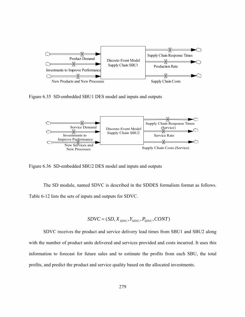
279
Figure 6.35 SD-embedded SBU1 DES model and inputs and outputs
Figure 6.36 SD-embedded SBU2 DES model and inputs and outputs
The SD module, named SDVC is described in the SDDES formalism format as follows.
Table 6-12 lists the sets of inputs and outputs for SDVC.
),,,,( CONTPYXSDSDVC SDVCSDVCSDVC=
SDVC receives the product and service delivery lead times from SBU1 and SBU2 along
with the number of product units delivered and services provided and costs incurred. It uses this
information to forecast for future sales and to estimate the profits from each SBU, the total
profits, and predict the product and service quality based on the allocated investments.
Discrete-Event ModelSupply Chain SBU1
Product Demand
Production Rate
Supply Chain Costs
Supply Chain Response Times
Investments to Improve Performance
New Products and New Processes
Discrete-Event ModelSupply Chain SBU2
Service Demand Service Rate
Supply Chain Costs (Service)
Supply Chain Response Times (Service)
Investments to Improve Performance
New Services and New Processes

280
Table 6.12 Inputs and outputs of the SDVC module
MIOX
m vi sm msop mU
ip u t f SDVC LEAD_TIME1 SBU1 OP_SBU1_01 IP_SDVC_01 PROFITS1 TB_END NONE SDVC LEAD_TIME2 SBU2 OP_SBU2_01 IP_SDVC_02 PROFITS2 TB_END NONE SDVC PRODUCTS SBU1 OP_SBU1_02 IP_SDVC_03 SALES1 TB_END NONE SDVC SERVICES SBU2 OP_SBU2_02 IP_SDVC_04 SALES2 TB_END NONE SDVC TOTAL_COST1 SBU1 OP_SBU1_03 IP_SDVC_05 PROFITS1 TB_END NONE SDVC TOTAL_COST2 SBU2 OP_SBU2_03 IP_SDVC_06 PROFITS2 TB_END NONE
MIOY
m op vo
YmD
dm mdV
mdip vu t f
SDVC OP_SDVC_01 PRODUCT_DEMAND SBU1 IP_SBU1_01 PRODUCT_AR TB_START MISC_SD >> TB_BASED_RATE
SDVC OP_SDVC_02 SERVICE_DEMAND SBU2 IP_SBU2_01 SERVICE_AR TB_START MISC_SD >> TB_BASED_RATE
SDVC OP_SDVC_03 PRODUCT_QUALITY SBU1 IP_SBU1_02 REWORK_RATE TB_START NONE SDVC OP_SDVC_04 SERVICE_QUALITY SBU2 IP_SBU2_02 REJECT_RATE TB_START NONE
PRODUCTS: Number of product units delivered SERVICES: Number of services provided PRODUCT_DEMAND: Predicted order for product SERVICE_DEMAND: Predicted demand for service PRODUCT_AR: At USB1 to denote the order arrival rate at the module based on the SDVC input SERVICE_AR: At USB2 to denote the demand for service rate at the model based on the SDVC input REWORK_RATE: At USB1 to indicate the rejection rate of the product based on the current quality level REJECT_RATE: At USB2 to indicate the rate of failure to provide the service to the desirable standard, based on the current quality level MISC_SD >> TB_BASED_RATE: the SD input variable is a simple value and should be converted into the arrival rate of entities at the DES module for the TB length

281
The inputs from the DES modules are calculated by the modules in monetary values and
they are used without formatting at the SD module. The SBU1 module is described in the
SDDES formalism format as follows. Table 6-13 lists the sets of inputs and outputs for the
module.
),,,,(1 111 TBPYXDESUSB USBUSBUSB=
The SBU2 module is described in the SDDES formalism format as follows. Table 6-14
lists the sets of inputs and outputs for the module.
),,,,(2 222 TBPYXDESUSB USBUSBUSB=

282
Table 6.13 Inputs and outputs of the SBU1 module
MIOX
m vi sm msop mU
ip u t f
SBU1 PRODUCT_DEMAND SDVC OP_SDVC_01 IP_SBU1_01 PRODUCT_AR TB_START MISC_SD >> TB_BASED_RATE
SBU1 PRODUCT_QUALITY SDVC OP_SDVC_03 IP_SBU1_02 REWORK_RATE TB_START NONE
MIOY
m op vo
YmD
dm mdV
mdip vu t f SBU1 OP_SBU1_01 LEAD_TIME1 SDVC IP_SDVC_01 PROFITS1 TB_END NONE SBU1 OP_SBU1_02 PRODUCTS SDVC IP_SDVC_03 SALES1 TB_END NONE SBU1 OP_SBU1_03 TOTAL_COST1 SDVC IP_SDVC_05 PROFITS1 TB_END NONE

283
Table 6.14 Inputs and outputs of the SBU2 module MIOX
m vi sm msop mU
ip u t f
SBU2 SERVICE_DEMAND SDVC OP_SDVC_02 IP_SBU2_01 SERVICE_AR TB_START MISC_SD >> TB_BASED_RATE
SBU2 SERVICE_QUALITY SDVC OP_SDVC_04 IP_SBU2_02 REJECT_RATE TB_START NONE
MIOY
m op vo
YmD
dm mdV
mdip vu t f SBU2 OP_SBU2_01 LEAD_TIME2 SDVC IP_SDVC_02 PROFITS2 TB_END NONE SBU2 OP_SBU2_02 PRODUCTS SDVC IP_SDVC_04 SALES2 TB_END NONE SBU2 OP_SBU2_03 TOTAL_COST2 SDVC IP_SDVC_06 PROFITS2 TB_END NONE

284
Molding the DES modules contents was guided by the supply chain operations reference
(SCOR) model (Bolstorff and Reosenbaum, 2004). SCOR describes the business activities,
operations, and tasks in all steps of satisfying supply chain’s internal and external customer
demand. The three decision alternatives are described in the wider scope Figures 6-37 through 6-
39. It is noted that in all three alternatives, service units are kept in the continental USA since
consumers are located mainly in the continental USA.
Alternative A – SBU 1 under the organization (no outsourcing): As shown in Figure 6-
37, the manufacturing facility handles the sourcing of stocked raw materials (S1) from stocked
raw material suppliers (D1) and processes the make-to-order manufacturing (M2), the deliver-to-
order finished products (D2), the sourcing of returned defective products (SR1), the sourcing of
maintenance required operations (MRO) for sold products (SR2) from all local warehouses, and
the delivery of MROs back to warehouses (DR2). Moreover, the warehouse handles the sourcing
of make-to-order products from SBU 1 (S2), the delivery of the make-to-order products to end
customers (D2), the sourcing of returned defective products (SR1), the sourcing of MROs for
sold products (SR2) from customers, and the delivery of MROs back to customers (DR2).

285
Figure 6.37 SCOR representation of alternative A (no outsourcing)
Alternative B – Outsourcing SBU1 in South East Asia: As shown in Figure 6-38 all
process categories are similar to Alternative A, except that the manufacturing facility does not
handle MROs (SR2 & DR2) and product returns (SR1), as they are all handled locally at the
warehouses and service facilities. On the other hand, delivery of make-to-order products from
SBU 1 to local warehouses (D2) consumes a relatively longer duration due to maritime transport
and customs operations in California.

286
Figure 6.38 SCOR representation of alternative B
Alternative C – Outsourcing SBU1 to East Asia: As shown in Figure 6-39, all process
categories are similar to Alternative B, except that delivery of make-to-order products from SBU
1 to local warehouses (D2) consumes the longest duration in comparison to alternatives A and B.
Moreover, the local warehouse handles an extra QC inspection for the incoming products prior to
delivering to customers (D2).
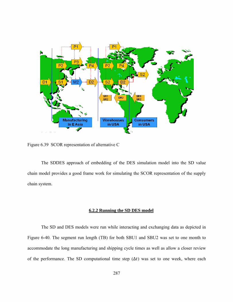
287
Figure 6.39 SCOR representation of alternative C
The SDDES approach of embedding of the DES simulation model into the SD value
chain model provides a good frame work for simulating the SCOR representation of the supply
chain system.
6.2.2 Running the SD DES model
The SD and DES models were run while interacting and exchanging data as depicted in
Figure 6-40. The segment run length (TB) for both SBU1 and SBU2 was set to one month to
accommodate the long manufacturing and shipping cycle times as well as allow a closer review
of the performance. The SD computational time step (∆ ) was set to one week, where each

288
month is four weeks long. When a DES input value is not updated yet the most recent available
value is used in the SD calculations. The SDDES controller actions sequence to synchronize the
modules is indicated by the numbers on the arrows in Figure 6-40.
At the beginning of the simulation run SD exports the estimates of product and service
demand for the coming period and the affordable quality levels to the DES modules. Upon
completing each run segment, the DES model provides estimates of the costs associated with
meeting the orders for products or services and the number of units delivered with the lead time
and rejection levels for the current quality standards. SD uses the DES inputs to updates its
estimates of the system performance, profits from each business unit and the total profits, and the
level of customer satisfaction. Based on the profits realized investments in production equipment
and service staff and capabilities are decided and the expected level of quality can be predicted.
The analysis is conducted for a five year period, for each of the outsourcing alternatives. The
overall performances from the three alternatives are compared with respect to profits realized,
responsiveness, and the customer satisfaction.

289
tΔ
Figure 6.40 sequence of synchronizing the SD and DES modules
6.2.3 Simulation results and analysis
The five-year analysis period showed that keeping both the manufacturing and service
facilities in the continental USA leads to the best level of responsiveness. However, due to high
overhead, profits are not expected before the third year and during that period the customer
satisfaction will fall significantly. Meanwhile the two outsourcing options can lead to higher
levels of profits and good stable customer satisfaction rates despite the low performance in terms
of responsiveness. Figures 6-41 through 6-43 compare the three alternatives with respect these
measures of performance.

290
Figure 6.41 Comparing outsourcing alternatives with respect to profits
Figure 6.42 Comparing outsourcing alternatives with respect to customer satisfaction rate

291
Figure 6.43 Comparing alternative with respect to manufacturing lead time
The simulation results provided insights on the expected performance of the system under
the outsourcing alternative in considerations. The results provided the decision makers with
inputs to make the decision. Yet to further support the decision makers and incorporate their
experiences of the global economy, a stochastic AHP framework (Rabelo et al., 2007; Eskandary
and Rabelo, 2006) was used. With AHP utilizing the simulation model outputs, decision makers
can build on their experiences and consider relevant tradeoffs (political, social, technical, etc) in
making the final decision. This also increases the decision makers’ confidence in the expected
outcomes.
For the value chain system, three decision makers – Chief Financial Officer, Chief
Operations Officer, and Vice-President of Sales/Marketing – engage in the strategic decision
making process by expressing their preferences. The weighted geometric mean method (Aull-

292
Hyde et al., 2006, Forman and Peniwati, 1998) is employed to estimate global weight of
participant preferences while minimizing inconsistencies. All participants are weighted equally
and the stochastic AHP approach is applied to the aggregated group estimates rather than
individual estimates. Investigating the 95% confidence intervals of the global weights gained by
the stochastic AHP methodology (Figure 6-44), it is noticed that there is considerable overlap
between alternatives A and C.
The apparent ranking of the alternatives is B, A, then C. But the overlap between A and C
indicates that they are tied and that further investigation is needed. Using the simulation of the
stochastic AHP methodology, the summary of output results of 10,000 replications is given in
Table 6-15. We can see that alternative B occupied the first place 99.99%. Alternative B does
dominate A and C. However, the summary shows that alternative A and C ranked second 77.5%
and 22.5% of the time, respectively, indicating that the null assumptions that alternative A is
probabilistically superior to alternative C is rejected.
Using the stochastic AHP analysis with the hybrid simulation outputs could confirm the
decision that outsourcing the manufacturing facility as in Alternative B in the best choice for the
current value chain system over the planning horizon.
Table 6.15 Simulation results of the stochastic AHP for ranking the outsourcing alternatives
Rank Rank
Alternative 1 2 3 1 2 3 A 1 7747 2252 ≈0.0% ≈77.5% ≈22.5%B 9999 1 0 ≈100% ≈0.0% 0.0% C 0 2253 7747 0.0% ≈22.5% ≈77.5%
Totals 10000 10000 10000 100% 100% 100%

293
Figure 6.44 Global weights of the outsourcing alternative based on the stochastic AHP analysis
6.3 Comparing SDDES and AnyLogic
This section presents the results of comparing a hybrid simulation model of SD and DES
units built using AnyLogic with the same model built using the SDDES framework. AnyLogic is
being marketed as the only commercial simulation package that combines comprehensive DES
and SD simulation building tools in the same interface with the ability to combine them. The
objective of the comparison is benchmarking SDDES with AnyLogic as well as providing
insights about how AnyLogic implements the interactions between SD and DES.
As discussed in Chapter 2, AnyLogic implemented the hybrid state machine process
(Maler et al, 1992, Harel, 1987) to provide tools to build hybrid discrete and continuous
simulations. Objects for traditional DES simulation and dynamic variables for SD modeling are
accessible from within the same user interface. Yet AnyLogic users need to be Java
programmers. Technically, AnyLogic is a Java programming interface that offers pre-designed
0.50.3 0.4
A
BC Global
weight
Alternative
0.2

294
classes of objects for simulation purposes.
In conducting this study we contacted representatives of XJ Technologies; the vendors of
AnyLogic and requested them to demonstrate interfacing SD and DES models in AnyLogic.
They recommended using the dynamic event object (See Chapter 2) and provided an AnyLogic
model that used the dynamic event to interface a SD and a DES objects. This model is based on
the classical pass diffusion model with added DES objects. Although this AnyLogic model
included a stochastic DES part, it used AnyLogic’s default simulation experiment, which allows
for a single simulation run replication only. For statistical validity we also requested them to
demonstrate replicating the DES unit. But since the default simulation experiment in AnyLogic
does not allow replication, they recommended writing Java code to replicate the stochastic DES
model part. A Java repetition construct (e.g. FOR or WHILE-DO structure) can be used to
control the simulation experiment and replicate the DES part of the hybrid SD-DES model.
Using Java required separating the SD and DES parts into separate objects.
AnyLogic does not provide any particular support to synchronizing a deterministic SD
model and a replicated stochastic DES model. But as a programming language interface and
since many objects can be included in the model, modelers can resort to their programming skills
to design any special simulation run scenarios.
The AnyLogic model was modified to use a For-loop statement for replicating the DES
object as will be described later. We then built an equivalent SDDES model and compared the
results generated by it to the results generated by the AnyLogic model.
The DES models can be built in AnyLogic using the enterprise library (a collection of

295
objects representing the common elements used in the traditional flowchart-based DES
simulation modeling). SD models can be built using the stocks and flow rate variables (called
dynamic variables). In its current version 6.0, AnyLogic allows two approaches to interface the
SD variables and the DES objects:
1. Using the statechart object: state charts are defined within an object to control its
behavior. The transition from a state to a state is a timeless discrete event that can be
triggered by changes in the state of the system (the occurrence of other events) or based
on the advance of the simulation time. To incorporate the continuous behavior, Java code
that references one or more continuous variables can be linked to a transition or a state
(See Chapter 2) to trigger an event to take the transition or update the system state based
on the values of the continuous variables.
2. Using the dynamic event object: this special type of event was added in AnyLogic 6 as a
simplified form of using the statechart. The dynamic event object can be scheduled to
occur as a reaction to a condition that has just been met, or to act at specified points in
time, in such case it is used as a timer. The action to be taken is defined in the event using
java.
Further, since the SD variables in AnyLogic are treated as variable not objects, these
variables can be directly referenced in the mathematical formulas or within the code used in any
other object in the simulation model as indicated.
AnyLogic models are run by the execution of an instance of the object class Experiment.

296
The default simulation experiment does not allow replications in the simulation run. The
parameter variation experiment can be added to the model to execute several single model runs
while varying one or more root object parameters within specified ranges, for comparative and
sensitivity analysis purposes. The optimization experiment can be used to perform performance
and design optimization analysis. Using Java, users can also define custom experiments, which is
the case in the current comparative discussion.
Thus, AnyLogic provides no support to develop hybrid SD-DES simulation as described
in the SDDES framework except by using Java. In the following subsections, we compare the
AnyLogic model to an equivalent SDDES model. The purpose of the comparison is to
demonstrate the potential of SDDES to synchronize the separate SD and DES modules and
simplify the model building process.
6.3.1 The AnyLogic model
As shown in Figure 6-45, AL represents a hypothetical supply and demand situation,
where the demand for a certain product is modeled in SD while the supply is modeled in DES;
forming a closed feedback loop. The variables in the SD section of the model are defined below:
• PotentialAdopters: the total population who under the effect of advertisement
generate demand for the product.
• Demand: the current unmet demand for the product
• AdEffectivness: the level of effectiveness of advertisement; convincing
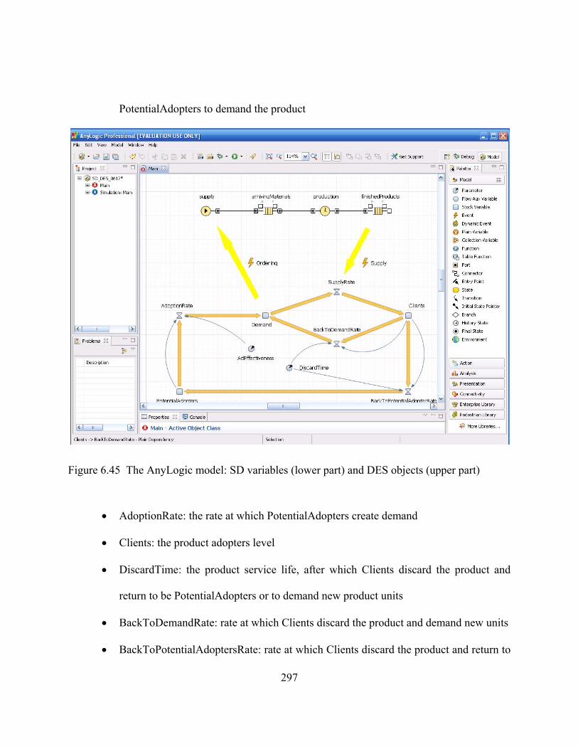
297
PotentialAdopters to demand the product
Figure 6.45 The AnyLogic model: SD variables (lower part) and DES objects (upper part)
• AdoptionRate: the rate at which PotentialAdopters create demand
• Clients: the product adopters level
• DiscardTime: the product service life, after which Clients discard the product and
return to be PotentialAdopters or to demand new product units
• BackToDemandRate: rate at which Clients discard the product and demand new units
• BackToPotentialAdoptersRate: rate at which Clients discard the product and return to

298
the general population.
• SupplyRate: rate at which adopters move from Demand to Clients.
The SupplyRate represents the rate of decrease of the Demand and the rate of increase of
the Clients. It is input from the DES section of the model which in turn receives the Demand
level as the input.
The objects in the DES section are defined below:
• supply: a source object that cause the creation of the entities (raw materials units) in
at the production line. It is driven by the Demand level provided by the SD section.
• arrivingMaterials: a queue object where new arriving materials can wait until the
availability of the production resources.
• production: a delay object to model the processing delay of the material units.
Materials are delayed for the specified processing time before they can proceed
• finishedProducts: a queue object where final product units may wait until pulled to
the SupplyRate in the SD section.
The interactions between the SD and DES are implemented using the two dynamic event
objects: Ordering and Supply shown in Figure 6-45. The ordering event communicates the
Demand level to the production facility (DES) at the beginning and middle of each workday. The
Demand level becomes the number of arriving material units at the supply object. The Sales

299
event communicates the number of final product units at the production facility to the
SupplyRate variable at the SD section. This is done at the middle and end of each workday.
Thus the model works by following the three overlapping negative causal loops shown in
Figure 6-46. This causal loop diagram also applies to the SDDES model.
1. Loop 1: Higher level of potential adopters creates a higher level of demand which
increases ordering at the production facility. Production and consequently the clients
level will increase. The increase in clients decreases the potential adopters’ level.
2. Loop 2: Higher level of demand increases ordering at the production facility to
increase production and consequently increases the clients level. The increase in
clients decreases the demand level.
3. Loop 3: the higher the demand the higher the clients level but as the clients level
increases the demand level will decrease.
Since this AnyLogic model can only run for a single replication it does not give
statistically valid results. If the model is run for a number of times using different streams of
random numbers each time, an independent set of data samples can be generated to perform
useful statistical analyses. This forces the deterministic objects in the model to be replicated as
well. More statistical analysis and programming efforts will be needed to collect the output and
perform the output analysis of the results.

300
Figure 6.46 Overlapping causal loops in the AnyLogic model. The shaded box; Product Units indicate the DES section of the model
6.3.2 Replicated DES object in the AnyLogic model
We asked the XJ Technologies representatives to demonstrate running their AnyLogic
model such that only the DES section is replicated. They used the Java for-loop programming
structure for that purpose. In order to replicate DES, it has to be isolated in a separate object in
the simulation model. The DES and SD parts in Figure 6-45 were separated in two objects. The
SD object was designated as the main root object for the simulation run experiment. While SD is
running, a dynamic event object executes the for-loop code to instantiate the DES object,
instantiate the simulation engine object, run the DES instance, and then destroy all object
PotentialAdopters
Demand
Ordering
Product Units
Clients+
+
+
+
-
-+Loop 3
Loop 2
Loop 1
301
instances in each loop. Meanwhile the object is collecting the discrete data. Each loop thus
represents a replication. The pseudo code implementing the looping structure to run the DES
object for a number of replication from within the run of the SD object is listed below. This
pseudo code uses AnyLogic’s Java methods and functions. It can be used in the action section of
a dynamic event, which should be added to the SD object. The replication counter is i while reps
is used to denote the number of replications. Engine is the AnyLogic simulation engine object
class and engine is an instance. DES is the discrete simulation object and des is an instance. The
runFast()method is a Java method applies to the Engine object and causes the DES object
instance to run in the virtual time.

302
for ( int i=0; i<reps; i++ ) { // create a new engine instance Engine engine = new Engine(); // create a new DES model instance to run DES des = new DES( engine, null, null ); // actions before running model instance
.... .... .... // start and running the DES instant engine.start( des ); engine.runFast(); // actions before end of run # i .... .... ....
// end run # i and destroy model instant engine.stop();
}
// actions for all replications (collecting model outputs) .... .... ....
6.3.3 The hybrid SDDES model
The equivalent SDDES model made use of the SDDES controller testbed described in
Chapter 5. Figures 6-47 and 6-48 show the SD and the DES modules respectively (Using Vensim
and Arena respectively). The SDDES model matches AL as described in Table 6.16

303
Figure 6.47 The SD module of the SDDES model

304
Figure 6.48 The DES module of the SDDES model

305
Table 6.16 Corresponendence between the AnyLogic and the equivalent SDDES models Model
Element AnyLogic SDDES
SD Potential Adopters
Stock variable changing by the net effect of the inflow BackToPotentialAdoptersRate and outflow AdoptionRate flow rates. Units: Person
Stock variable changing by the net effect of the inflow Back To Potential Adopters Rate and outflow Adoption Rate flow rates. Units: Person
Advertising effectiveness
Parameter AdEffectiveness = 0.01 Dimensionless
Constant Ad Effectiveness = 0.01 Dimensionless
Product adoption rate
Flow rate variable AdoptionRate = (PotentialAdopters)(AdEffectiveness) Units: Person / day
Flow rate variable Adoption Rate = (Potential Adopters)(Ad Effectiveness) Units: Person / day
Demand Stock variable changing by the net effect of inflows AdoptionRate and BackToDemandRate and outflow SupplyRate. Units: Person
Stock variable changing by the net effect of inflows Adoption Rate and Back To Demand Rate and outflow Supply Rate 1. Units: Person
Clients Stock variable changing by the net effect of the inflows SupplyRate and outflows BackToPotentialAdoptersRate and BackToDemandRate Units: Person/day
Stock variable changing by the net effect of the inflows Supply Rate and outflows Back To Potential Adopters Rate and Back To Demand Rate Units: Person/day
Product discard rate w/o demand
Flow rate variable BackToPotentialAdoptersRate; function in Clients level and DiscardTime Units: Person / day
Flow rate variable Back To Potential Adopters Rate; function in Clients level and Discard Time Units: Person / day
Product discard rate w/ demand
Flow rate variable BackToDemandRate; function in Clients level and DiscardTime. Units: Person / day
Flow rate variable BackToDemandRate; function in Clients level and DiscardTime. Units: Person / day
Product useful service life
Parameter DiscardTime = 10 Units: day
Constant Discard Time = 10 Units: day
Production supply
Flow rate variable SupplyRate that is function in input from the DES unit Units: Person/day
Flow rate variable Supply Rate that is function in input from the DES unit. Flow rate variable Supply Rate 1 is used as outflow to Demand while Supply Rate is used as inflow to Clients. The two flow rates are equal and both are based on DES input. Units: Person/day
DES Entities creation
Source object supply that creates a number of entities equal to the imported value of the Demand level
Create module Supply that creates a number of entities equal to the imported value of the Demand level
Raw materials storage
Queue object arrivingMaterials. Entities wait until production capacity units are available at the production object. Entities then proceed to use available capacity
Seize module Seize Production Resource. Entities wait at the module’s queue until resource units are available at the Production module. Entities are matched with available resource units then they proceed.

306
Model Element AnyLogic SDDES
DES Production Delay object production where entities are
delayed for the specified processing time. Processing time is assigned at the delay module
Delay module Production where entities are delayed for the specified processing time. Processing time is assigned at the Assign module Assign Time.
Final product storage
Queue object finishedProducts where product units are stored until pulled to the SD model unit
Hold module Finished Products where product units are held in its queue until released by the SDDES controller to be exported to the SD module
Let the SD module of SDDES be referred to as SDmodule and the DES module be
referred to as DESmodule. In the SDDES formalism format, SDmodule is specified as follows:
),,,,(mod modmodmod CONTPYXSDuleSD uleSDuleSDuleSD=
The sets of inputs and outputs of SDmodule are presented in Table 6-17. The DESmodule
is expressed in the SDDES formalism as given below. The sets of inputs and outputs of
DESmodule are given in Table 6-18.
),,,,(mod modmodmod TBPYXDESuleDES uleDESuleDESuleDES=

307
Table 6.17 Inputs and outputs of the SDmodule module
uleSDX mod
m vi sm msop mU
ip u t f SDmodule FINISHED
PRODUCTS DESmodule OP_DESmodule_01 IP_SDmodule_01 SUPPLY
RATE TB OBSERVATIONAL_DES_TB
>> TB_BASE_TIME_RATE
SUPPLY RATE 1 TB
OBSERVATIONAL_DES_TB >> TB_BASE_TIME_RATE
uleSDY mod
m op vo
YmD
dm mdV
mdip vu t f SDmodule OP_SDmodule_01 DEMANDi DESmodule IP_DESmodule_01 DEMAND
SIZE STARTUP NONE
SDmodule OP_SDmodule_02 DEMAND DESmodule IP_DESmodule_02 DEMAND SIZE
TB NONE
FINISHED PRODUCTS: number of finished product units as given by the Finished Products module in DESmodule SUPPLY RATE: the flow rate variable Supply Rate in the SDmodule SUPPLY RATE 1: the flow rate variable Supply Rate 1 in the SDmodule OBSERVATIONAL_DES_TB >> TB_BASE_TIME_RATE: input variable is based on observational data from DES that was collected over TB, and should be converted into a rate variable over the simulation base time unit to be usable in SD. DEMANDi: initial demand level DEMAND: the current Demand stock level DEMAND SIZE: corresponding demand level variable at DESmodule

308
Table 6.18 Inputs and outputs of the DESmodule module
uleDESX mod
m vi sm msop mU
ip u t f DESmodule DEMANDi SDmodule OP_SDmodule_01 IP_DESmodule_01 DEMAND
SIZE STARTUP NONE
DESmodule DEMAND SDmodule OP_SDmodule_02 IP_DESmodule_02 DEMAND SIZE
TB NONE
uleDESY mod
m op vo
YmD
dm mdV
mdip vu t f DESmodule OP_DESmodule_01 FINISHED
PRODUCTS SDmodule IP_SDmodule_01 SUPPLY
RATE TB OBSERVATIONAL_DES_TB
>> TB_BASE_TIME_RATE SUPPLY
RATE 1TB OBSERVATIONAL_DES_TB
>> TB_BASE_TIME_RATE

309
6.3.4 Comparing SDDES to AnyLogic
The models were set to simulate the performance of the system on a daily basis. The SD
and DES modules/objects exchange the demand and production level. The current demand and
current production are updated twice a day. For the simple AnyLogic model (Figure 6-45), the
dynamic event Ordering updates the DES model part with the current demand level every 0.5
day starting at time zero. Demand level is inserted at the source object supply as the number of
material units to be processed. The dynamic event Supply checks for the availability of the
finished product units at the finishedProducts object, and for the demand level value. It matches
demand and production and communicates the current production rate to the SD flow rate
variable: SupplyRate to update the Demand and Clients stocks.
When the looping structure is implemented, the DES is removed to a separate object. The
dynamic event Ordering (in the SD object) is scheduled to occur every 0.5 time units starting at
time zero, to perform the instantiation of the DES object and the simulation engine and to run the
discrete instance for 30 replications. The event collects the production rate data and the state of
the production line at the end of the object instance run.
Since the DES is required to provide productivity data every 0.5 time unit, the DES
instance of the object and the simulation engine instance are destroyed upon completing the 30
replications. By default the DES instance would run for the entire simulation run length. In the
current analysis, the simulation model is run for 100 days while interactions between the objects

310
are executed every 0.5 day. The DES object instance will run for 100 days in each replication
unless the object is destroyed at time 0.5. In AnyLogic the simulation run length is set for the
experiment object and it affects all objects referenced in the experiment. AnyLogic does not
allow running more than one experiment at a time.
Further, and since the dynamic events in AnyLogic are discrete, their occurrences are
timeless. Once the replications of the DES object instance are completed the simulation
experiment’s focus returns to the SD object. Although DES may contain discrete objects that
perform time-consuming tasks (e.g. processing) the focus of the simulation run returns to the SD
object at the same point in time when the event occurred. The DES object is not aware of the
simulation time. Programmed delays must be included in order to instruct the SD object not to
use the DES inputs until the correct time to use them. In the SDDES framework, synchronizing
the modules run and the use of data is controlled completely by the SDDES controller.
To compare the SDDES model and the AnyLogic model, the models were run for a
period of 100 days. The TB for the DESmodule of SDDES was set at 0.5 day and 30 replications
were performed in each segment. The dynamic events in the AnyLogic model were scheduled to
occur every 0.5 days. The Java for-loop subroutine in the AnyLogic model was set to perform 30
replications. The Demand, Clients, and Potential Adopters levels were monitored for the two
models. The initial potential adopters’ population is 1000. The initial Demand level is five. The
initial Clients level is zero. The ad effectiveness constant is 0.01 and the product useful service
time is 10 days. It is assumed that any unused final product units are discarded.

311
6.3.5 Results and discussion
Figures 6-49 through 6-51 compare the levels of Demand, Clients, and Potentials
Adopters for the AnyLogic and SDDES models. The results show similar and equivalent results
from the two simulations. The 2-sample t-test for the difference between the means shows no
evidences at 95% confidence level, to reject the null hypothesis that the results from the two
simulations are equivalent. The test results are shown in Tables 6-19 through 6-21.
Figure 6.49 Equivalent demand level and behavior from SDDES and AnyLogic
0.00
2.00
4.00
6.00
8.00
10.00
12.00
0.0
3.0
6.0
9.0
12.0
15.0
18.0
21.0
24.0
27.0
30.0
33.0
36.0
39.0
42.0
45.0
48.0
51.0
54.0
57.0
60.0
63.0
66.0
69.0
72.0
75.0
78.0
81.0
84.0
87.0
90.0
93.0
96.0
99.0
Time
Demand Level ‐ SDDES Model
0
2
4
6
8
10
12
0.0
3.0
6.0
9.0
12.0
15.0
18.0
21.0
24.0
27.0
30.0
33.0
36.0
39.0
42.0
45.0
48.0
51.0
54.0
57.0
60.0
63.0
66.0
69.0
72.0
75.0
78.0
81.0
84.0
87.0
90.0
93.0
96.0
99.0
Time
Demand Level ‐AnyLogic Model

312
Figure 6.50 Equivalent clients level and behavior from SDDES and AnyLogic
0
25
50
75
100
125
1500.0
3.0
6.0
9.0
12.0
15.0
18.0
21.0
24.0
27.0
30.0
33.0
36.0
39.0
42.0
45.0
48.0
51.0
54.0
57.0
60.0
63.0
66.0
69.0
72.0
75.0
78.0
81.0
84.0
87.0
90.0
93.0
96.0
99.0
Time
Current Clients ‐ SDDES Model
0
25
50
75
100
125
150
0.0
3.0
6.0
9.0
12.0
15.0
18.0
21.0
24.0
27.0
30.0
33.0
36.0
39.0
42.0
45.0
48.0
51.0
54.0
57.0
60.0
63.0
66.0
69.0
72.0
75.0
78.0
81.0
84.0
87.0
90.0
93.0
96.0
99.0
Time
Current Clients ‐AnyLogic Model

313
Figure 6.51 Equivalent potential adopters level and behavior from SDDES, AL_1, and AL_2
840860880900920940960980
1,0000.0
3.0
6.0
9.0
12.0
15.0
18.0
21.0
24.0
27.0
30.0
33.0
36.0
39.0
42.0
45.0
48.0
51.0
54.0
57.0
60.0
63.0
66.0
69.0
72.0
75.0
78.0
81.0
84.0
87.0
90.0
93.0
96.0
99.0
Time
Potential Adopters ‐ SDDES Model
840860880900920940960980
1,000
0.0
3.0
6.0
9.0
12.0
15.0
18.0
21.0
24.0
27.0
30.0
33.0
36.0
39.0
42.0
45.0
48.0
51.0
54.0
57.0
60.0
63.0
66.0
69.0
72.0
75.0
78.0
81.0
84.0
87.0
90.0
93.0
96.0
99.0
Time
Potential Adopters ‐AnyLogic Model

314
Table 6.19 2-sample t-test for the difference between mean demand levels – SDDES and AnyLogic Two-sample T for SDDES vs AnyLogic N Mean StDev SE Mean SDDES 201 6.213 0.939 0.066 AnyLogic 201 6.189 0.935 0.066 Difference = mu SDDES - mu AnyLogic Estimate for difference: 0.0238 95% CI for difference: (-0.1599, 0.2075) T-Test of difference = 0 (vs not =): T-Value = 0.25 P-Value = 0.799 DF = 399
SDDES AnyLogic
2
3
4
5
6
7
8
9
10
11
Boxplots of SDDES and AnyLogic(means are indicated by solid circles)
SDDES AnyLogic
2
3
4
5
6
7
8
9
10
11
Dotplots of SDDES and AnyLogic(means are indicated by lines)

315
Table 6.20 2-sample t-test for the difference between mean clients levels – SDDES and AnyLogic Two-sample T for SDDES vs AnyLogic N Mean StDev SE Mean SDDES 201 98.5 23.7 1.7 AnyLogic 201 98.5 23.7 1.7 Difference = mu SDDES - mu AnyLogic Estimate for difference: 0.02 95% CI for difference: (-4.63, 4.67) T-Test of difference = 0 (vs not =): T-Value = 0.01 P-Value = 0.994 DF = 399
SDDES AnyLogic
0
50
100
Boxplots of SDDES and AnyLogic(means are indicated by solid circles)
SDDES AnyLogic
0
50
100
Dotplots of SDDES and AnyLogic(means are indicated by lines)

316
Table 6.21 2-sample t-test for the difference between mean demand levels – SDDES and AnyLogic Two-sample T for SDDES vs AnyLogic N Mean StDev SE Mean SDDES 201 900.0 23.7 1.7 AnyLogic 201 900.2 23.8 1.7 Difference = mu SDDES - mu AnyLogic Estimate for difference: -0.13 95% CI for difference: (-4.79, 4.53) T-Test of difference = 0 (vs not =): T-Value = -0.06 P-Value = 0.956 DF = 399
SDDES AnyLogic
900
950
1000
Boxplots of SDDES and AnyLogic(means are indicated by solid circles)
SDDES AnyLogic
900
950
1000
Dotplots of SDDES and AnyLogic(means are indicated by lines)

317
It is concluded that the SDDES hybrid simulation framework can compare to AnyLogic
for integrating SD and DES simulations. SDDES could generate equivalent outputs to AnyLogic.
Further, it could integrate autonomous simulations built using different software without
necessitating additional programming efforts (as does AnyLogic) or modifications to the
simulation models
Synchronizing SD and DES model objects in AnyLogic requires advanced programming
skills (using Java) even when working inside the same environment. The use of discrete events
(the dynamic event object or the state chart triggered actions) necessitates introducing
information delays for the correct timing of using the data generated by the DES objects. Since
the dynamic events as all events, are discrete and their occurrences of events are timeless, the
instance of any DES objects running within the execution of the event cannot be aware of the
simulation time (assuming using a looping structure as in this section). All data generated by the
DES object instance will be returned to the simulation experiment (and the calling SD object) at
the same point in time when the DES object was instantiated. A forced programmatic
information delay is needed to delay using the DES data to the right point in time.
Easier synchronization would be possible if each DES and SD object could be run in a
separate AnyLogic experiment object such that the run time can be set for each separately and
data exchange transactions can be simpler. However, AnyLogic does not allow running more
than one experiment at the same time. In response to our quest to whether Java can be used to
allow parallel experiments, the head of the consulting department at XJ Technologies (an
AnyLogic modeler and Java programmer) stated that “I would not go into any parallel execution

318
for now due to its implementation is more difficult”.
It is worth noting that XJ Technologies stopped supporting HLA’s RTI for synchronizing
separate simulations in AnyLogic 6.0. Instead, Java programmers can use Java to develop and
utilize tools based on the TCP/IP protocols to synchronize such simulation objects. Stopping the
support for HLA/RTI follows a trend among simulation software vendors who do not see
demand for using HLA/RTI in the manufacturing and industrial applications (See Boer, 2006a,
and Poer, 2006b).
Thus we can conclude that SDDES can compare to AnyLogic in integrating SD and DES
models and unlike AnyLogic, modelers and users of SDDES do not need to learn new modeling
skills and they need no programming efforts to achieve the integration. Moreover, autonomous
SD and DES simulations built using different software packages can be interfaced using SDDES.
Existing/legacy simulation models can be used with SDDES without any specific modifications
to them.
6.4 The Control Function of SDDES
The stated purpose of using SDDES is the management policy design and testing. As a
simulation model, the uses of the SDDES model are not limited to policy design. The control
function is the first that should be mentioned. The common uses of simulation in the
manufacturing system control applications are focused at the operational/shop floor level and are
generally concerned the ability to monitor the system on the short term basis (commonly in
319
realtime) and the scheduling/rescheduling situations in response to uncertainties at the schedule
execution levels (Jones et al., 2001; Cowling and Johansson, 2002; Aytug et al, 2005; Son et al,
2005; Cho et al., 2006; Sinreich and Shints, 2006; Pfeiffer et al., 2008).
SDDES has been designed such that it maintains the integrity of the SD and DES
simulation methodologies. Thus, in addition to the ability of the SDDES to develop
comprehensive simulations of the manufacturing system and explain its behavior, the feedback
loops in SDDES can provide the tools to assess the ability of the system to perform self-control
and act to handle the deviations from the desired levels of behavior due to unexpected events at
the operational or at the aggregate level as well. This can indicate if the system is adequately
robust and well-structured.
In this section we discuss the control applicability of SDDES to the manufacturing
system, with a focus on the designing a self-control capability in the simulation model.
6.4.1 Decoupling the SD and DES modules
It has been shown in section 6-1 that the exchange of data between the SD and DES
modules allowed the system to react to unexpected shortages in production at the shop floor. The
weekly planned material usage and desired production rates along with the assigned capacity and
other operational settings were estimated and decided by SD and communicated through the
controller to the PREF and PRES modules. Daily feedback from PREF and PRES provided the
basis for the SD to assess the performance and update its estimates. Figure 6-29 (section 6-1)

320
showed that the finished goods inventory level could be adjusted when it was found to fall below
the desired level to support the planned shipping performance. In such situations, extra raw
materials were ordered and released at the production lines to increase productivity for the
inventory level to recover to equilibrium and maintain the desirable shipping performance.
In this section, the SD and DES modules are decoupled. The estimated customer order
rate, desired shipping and productivity performance, and the allocated resources are decided at
the beginning of the planning horizon at SD. The DES modules are run to execute the plan but
and they provide their feedback data to SD. SD is assumed to be unable to react to the deviations
in DES until the end of the planning horizons (s quarter). The performance of the system was
observed for the finished inventory and shipping performance.
Figure 6-52 describes the interactions between the SD and DES modules in the decoupled
run of SDDES. The SD modules are allowed to interact as described in section 6-1. Initial system
settings are provided by the SD modules for the PREF and PRES modules. Feedback from DES
is not reacted to by SD. Instead the planned material usage, production, and shipping rates hold
during the planning horizon. The * in variables names indicate initial values estimated at the
beginning of the planning horizon and are expected to hold valid. This creates an open feedback
loop structure between the SD and DES modules.

321
Figure 6.52 Data exchanged between the SD and DES modules – open feedback loop communications
6.4.2 Results and implications
Figure 6-53 shows the behavior of the final product inventory relative to the customer
order rate. As was the case in section 6-1, the inventory level fell short of the customer order rate
after the first week. By comparing Figure 6-53 with Figure 6-29 in section 6-1, it is observed that
the system could correct itself within one and a half week (Figure 6-29) when SD was able to
react to the deviations from the planned product and inventory level. When no control
performed, the system could recover the inventory level to the customer order rate in three work
weeks (Figure 6-53).

322
Figure 6.53 Final product inventory level and shipping performance – Decoupled SDDES
The drop in the product inventory level is caused by the sharp drop in production in the
PREF and consequently in PRES as shown by Figure 6-54. The recovery of the inventory level
to the customer order rate is driven by the fluctuating productivity on PREF. And since PRES is
run a pull system and it pulls preforms based on the current customer order then it does not
exceed the stated customer order rate and the system is never able to make up for the unshipped
products. It is assumed for the purpose of this experiment that no correction actions are by SD.
This in fact, gives more credit to SDDES as used in section 6-1 since it could easily capture the
system’s natural behavior represented by reactions of the decision makers.
Final Product Inventory and Shipping Perfomance8,000 units/week8,000 units1,000 units/week8,000 units/week
4,000 units/week4,000 units
0 units/week4,000 units/week
0 1 2 3 4 5 6 7 8 9 10 11 12Time (week)
Customer Order Rate : SDDES units/weekFINISHED GOODS INVENTORY : SDDES unitsUnshipped : SDDES units/weekDesired shipping : SDDES units/week

323
Figure 6.54 Production rates from PREF and PRES - Decoupled SDDES
As production is designed to meet the current customer order rate (raw materials from SD
are from the current customer order rate only), the unshipped products accumulate as shown in
Figure 6-53. Compared to Figure 6-29 in section 6-1, it is clear how the correction control
actions at the SD level could drive the system to handle the unshipped products. Further, without
the control effect the system is unable to respond to the customer orders on time and the delivery
delay builds up as shown in Figure 6-55. A delay of up to 20% (compared to about 5% in Figure
6-30 in section 6-1) in the quoted delivery delay is experienced and it continues to increase.
Production Rates20,000 units/week20,000 units/week
10,000 units/week10,000 units/week
0 units/week0 units/week
0 1 2 3 4 5 6 7 8 9 10 11 12Time (week)
Preforms Production Rate : SDDES units/weekPresses Production Rate : SDDES units/week

324
Figure 6.55 Delivery delay performance - Decoupled SDDES
In addition, the raw materials inventory level shows an increasing trend (Figure 6-56).
This is driven by the scheduled production rate as also shown in Figure 6-56. The scheduled
production rate in the PWS module is estimated to respond to the current customer order rate and
to any unshipped orders. As the unshipped orders accumulate the scheduled production rate
increases. Had the scheduled production been communicated to the PREF module, the system
would have corrected its product inventory level and decreased or eliminated the delayed orders.
This is compared to Figure 6-31 in section 6-1 in which the raw materials inventory follows the
actual production performance at the shop floor in a responsive manner with less excess
inventory. The fluctuations in the scheduled production rate in Figure 6-56 are due to the
Delivery Delay1.5
1.375
1.25
1.125
10 1 2 3 4 5 6 7 8 9 10 11 12
Time (week)
Delivery Delay : SDDES week

325
behavior of the work-in-process levels of PREF and PRES.
Figure 6.56 Raw materials inventory level and scheduled production rate - Decoupled SDDES
In conclusion, it was shown that the SDDES simulation model, in addition to simulating
and providing explanation for the system behavior it could also provide insights on the
robustness of the system structure and management policies in effect. The potential of using
SDDES for robustness assessment and, possibly, longer term real-time control has been
highlighted. A potential use of SDDES in relation to the real-time control application would be
accumulating knowledge and developing libraries of reference modes (by running the model for
different settings) of the system behavior for the planning horizon. The reference modes can be
Parts Inventory and Scheduled Production Rate15,000 units15,000 units/week
10,500 units10,500 units/week
6,000 units6,000 units/week
0 1 2 3 4 5 6 7 8 9 10 11 12Time (week)
PARTS INVENTORY : SDDES unitsScheduled Production Rate : SDDES units/week

326
used in conjunction with defining the threshold levels commonly used in the short term real-time
control systems to support the decision making process in reaction to the deviations from the
expected performance.
In section 6-1, it was shown that the PMO manufacturing system is designed adequately
well to correct itself whenever deviations from the planned performance occur and given that the
SDDES model captured the self-control capability of the system. However, due to the inherent
sources of fluctuations, the system undergoes periods of out-of control performance that can
persist and it cannot fully recover to equilibrium. Decoupling the SD and DES modules has
emphasized the effect of these sources of fluctuations and supported the analysis made in section
6-1.

327
CHAPTER 7: CONCLUSIONS AND DIRECTIONS FOR FUTURE RESEARCH
This research proposed a framework to integrate the SD and DES methodologies for
simulating the manufacturing enterprise system. This SDDES simulation framework can build
inexpensive, comprehensive, scalable simulations that support the management policy design
and analysis on an enterprise-wide level. This chapter summarizes the conclusions and
contributions of this research and highlights directions for future research.
7.1 Conclusions
Simulation modeling has been and will continue to be the most effective way for
analyzing the performance and designs of the manufacturing systems. But the evolution of the
manufacturing system and the continual changes in the business environment have created
serious challenges for the use of simulation in that area. This research asserts that the simulation
of modern manufacturing systems should be approached using hybrid tools that can incorporate,
in the same simulation, the operational and the aggregate management levels in a dynamic
feedback-based structure. They need to be comprehensive in scope, scalable, and able to
accommodate the continuous and discrete modes of behavior, the stochastic and deterministic

328
natures of the various business units, and the detail complexity and dynamic complexity
perspectives in the decision making processes. They also need to be practical to build and
inexpensive.
We have presented a definition of the scope of the manufacturing enterprise that consists
of five key components to cover the strategic, tactical, and operational functions and activities,
the external business environment, and the business “partners” (customers and suppliers). And it
could be justified to state that the existing simulation tools and frameworks (hybrid and
distributed simulations) fall short in meeting these characteristics of the simulation models of the
modern manufacturing enterprise system, for being based on certain assumptions that do not
make them able to accommodate all the decision making situations in the modern business
systems. We identified a gap in simulating the modern manufacturing enterprise system that is
not fulfilled by the existing simulation approaches.
This research proposed and developed a novel approach to integrate the system dynamics
(SD) and discrete event simulation (DES) paradigms in response to the indentified gap. The new
simulation framework (called the SDDES framework) utilizes SD for modeling the aggregate
management levels and DES for the detailed levels and facilitates the integration and
synchronization of them within a unified simulation arrangement (See Figure 7-1).

329
Figure 7.1 Layout of the hybrid SDDES simulation
The new framework consists of four main processes, namely the modularization,
resumption, formalization, and synchronization. By executing the four processes, separate SD
and DES simulations are interfaced and synchronized to be members of the comprehensive
SDDES simulation (See Figure 7-2). By modularization, autonomous SD and DES simulation
models are treated as modules in a more comprehensive simulation of the manufacturing
enterprise. The novel concept of resumption divides the DES run within the comprehensive
SDDES model into segments. Each segment is regular discrete simulation run with replications.
This allows the stochastic DES modules to be synchronized with the SD modules while
generating statistically valid data during the SDDES simulation run, not only at the end of the
run. Formalization uses the proposed SDDES formalism to provide a generic format for
specifying the SD and DES modules and their interactions, for the better management and easier
scalability of the simulation model. The SDDES synchronization algorithm provides the

330
mechanism for the data and information sharing between the modules.
Figure 7.2 The SDDES framework processes for integrating SD and DES simulations into unified SDDES model
The SDDES simulation framework processes are executed and managed by the SDDES
controller. The SDDES controller executes the data formatting and exchange transactions,
manages the simulation run, and provides the user/modeler interface to interact with the SDDES
model. The specific functions of the SDDES controller were described and an IDEF functional
model has been proposed.
The experimental analysis has shown that the new simulation framework has the potential
to enable modelers to develop simulation models that meet the requirements of
comprehensiveness, scalability, and the accommodation of the different modes of behavior and
needs of decision making processes at the different management levels. Two case studies of
using the proposed simulation methodology to simulate the manufacturing enterprise and the

331
manufacturing value chain have been conducted. It was concluded that the design of the SDDES
simulation framework is satisfactorily effective and efficient in modeling the manufacturing
enterprise and achieving the desirable characteristics in the simulation models.
The manufacturing system control applicability of the SDDES simulation framework has
been highlighted. SDDES was shown to be able to support the long term analysis of the
manufacturing system robustness and stability.
It was found that SD and DES when combined in a distributed-simulation-like
arrangement and synchronized in a way that maintains the integrity of each paradigm and avoids
one paradigm dominating the other, they can provide powerful tools to build the desirable
simulation models of the modern manufacturing enterprise. The SDDES simulation framework
was shown to facilitate this environment to integrate SD and DES.
Finally, the performance of the new SDDES methodology has been compared to the
available commercial hybrid simulation software and was found to generate equivalent
performance and results without requiring the modelers to learn new modeling and/or computer
programming skills as required by these software. Further, the new simulation framework can
utilizes the existing/legacy simulations without any particular modification in them.
7.2 Research Contributions
This research followed a unique approach to address a gap that has been identified in the
area of simulating the manufacturing enterprise system. Simulation modeling is known to be a

332
tedious, time consuming, and expensive process. And it is familiar that these simulations have
limited useful life spans since systems evolve, assumptions lose validity, and the objectives of
using the models could become obsolete. In addition, the desirable comprehensiveness with
respect to scope, view of the world, and accommodation of the different management levels’
perspectives and needs is hard to achieve. Dedicated simulation modeling languages have been
developed to enhance the efficiency of the simulation modeling process. Commercial software
packages have then been developed for more in that direction.
But the manufacturing system combines different types of behavior, perspectives, and
decision making situations. A single simulation tool cannot be adequate for modeling the total
system. Theorems, algorithms, and protocols to develop hybrid and distributed simulations have
been investigated and implemented to help and guide modelers in their efforts towards
comprehensiveness. Yet the outcomes have been of limited applicability in the manufacturing
applications.
This research has identified a need for new simulation modeling approaches that can
respond to the changing business environments towards more integration. These tools should be
able to develop comprehensive models that are inexpensive, scalable, and able to accommodate
the continuous and discrete modes of behavior, the stochastic and deterministic natures of the
various business units, and the detail complexity and dynamic complexity perspectives in
decision making.
In response to that gap in simulating the modern manufacturing system, the research has
proposed and developed a new simulation framework that combines the SD and DES simulation

333
paradigms. The new SDDES simulation framework is directed towards building hybrid
continuous-discrete simulation models in a distributed-simulation-like arrangement. These
models can satisfy the requirements in modeling the modern manufacturing systems. Combining
SD and DES accommodates the coexistence of the continuous and discrete behaviors and the
deterministic and stochastic natures in the system. They also accommodate the different
perspectives in decision making and views of the system being focused on the dynamic
complexity of the business unit or on the detail complexity in managing it. The comprehensive
and scalability dimensions in the simulation models of the manufacturing systems were achieved
by using a modular structure that regarded autonomous SD and DES models as modules
contributing to the same simulation. This also simplified the model building process as several
SD or DES modules can be built with well defined, relatively narrow scopes to model the
various business units and then be interfaced. The addition and deletion of the modules as the
system evolves over time is not restricted.
The research proposed and implemented a new synchronization algorithm that recognizes
and maintains the integrity of the two simulation paradigm of SD and DES. Unlike the existing
synchronization approaches the new algorithm is not driven by the occurrences of discrete
events.
This research also presented the concept of resumption to breakdown the DES simulation
run into segments, each is a complete traditional discrete simulation run with replications and
statistically valid structure and measures of performance. Resumption allows the DES modules
to offer statistically valid outputs at anytime during the simulation run; not only at the end of the

334
simulation run. This allowed stochastic, not only deterministic DES models to be interface with
SD models and exchange data and information over the planning horizons. An algorithm for
implementing the resumption of the DES models has been proposed and implemented in this
research.
Further, and for the purpose of better communications and model management, the
SDDES formalism has been introduced that provides a generic format to describe, specify, and
document the SD and DES modules. The SDDES formalism simplifies the modification of the
SDDES simulation model when needed and standardizes the interactions with the modelers/user
of the model.
The research presented and implemented the functional model of the SDDES controller
that implements the new simulation framework, manages the simulation model and simulation
run, and provides the user interface to interact with the simulation model.
It was shown that the components of the new simulation framework can be used to build
valid simulation models of the manufacturing system. A case study of a real manufacturing
system was presented. The experimental analysis also showed that the new simulation
methodology could generate equivalent results to commercial simulation software without
requiring any programming efforts or learning new simulation as required by these commercial
software packages.
This research contributed to the body of knowledge a view of the manufacturing
enterprise system that maps the various functions and decision making processes at the strategic,
tactical, and operational levels (See Figure 7-3) to SD or DES simulation modules. The modules

335
are specified by the proposed SDDES formalism that offers a generic format to characterize the
simulation models and the process they represent along with the data generated and used by each
allowing for integrating the simulation modules in a comprehensive model of the enterprise
system. Decision criteria to guide the mapping of the various business units to continuous or
discrete module are proposed.
Figure 7.3 Abstract representation of the manufacturing enterprise system
The research proposed a pioneering hybrid SD-DES simulation framework for simulating

336
the total enterprise system based on modularizing the business units as mentioned. The new
framework is comprehensive in accommodating all modes of behavior, perspectives, and scopes
in modeling and managing the manufacturing system business units. The new framework is
uniquely practical, flexible, inexpensive, and requires no new modeling or computer
programming skills. The
A new synchronization algorithm has also been contributed that is, to the best of our
knowledge, the first synchronization algorithm usable in the distributed simulation field that is
not discrete-event driven.
The research also contributed the functional model and implementation of the SDDES
controller for managing the synchronization and the simulation runs of the hybrid, distributed-
like simulations of the manufacturing enterprise system.
7.3 Directions For Future Research
We believe we have made a step forward yet we do not claim to have exhausted this
research area. Potential directions for more research to enhance and strengthen the SDDES
simulation framework’s usefulness and effectiveness can include the following:
• Enriching the SDDES synchronization mechanism by defining module interaction
control rules and criteria to improve the efficiency of the synchronization and overall
scalability of the SDDES simulation model. For applications that can involve
numerous modules behaving at varying dynamic levels better synchronization and

337
data and information sharing process can be achieved by optimizing the use of the
computing resources. This can include defining prioritization and significance
assessment criteria to guide the SDDES controller in performing its synchronization
function. Exchanging more data and information or more frequent information can be
expensive for the business and for the simulation model as well. Careful evaluation of
the benefits of sharing the information and the amount of information transfer versus
the associated cost should be made (Simchi-Levi et al, 2008). SDDES can benefit
from the Nyquist Sampling Theorem and Shannon’s information theory in
determining the appropriate level of information exchange frequency.
• Conducting more statistical analyses of the useful of the resumption process and how
it may improve the validity of the DES models as the system being modeled evolves
over time. Resumption offers an opportunity for modelers or other intelligent agents,
to modify the DES models during the simulation run in order to reflect the updated
system characteristic in the random distributions being uses in the models. This can
be done without losing the statistical validity of the data generated by the model “so
far” in the simulation run.
• Exploring the potential uses of SDDES for the long-range real time control of the
manufacturing systems at the strategic management level and the coordination with
the common short term real time control applicability of simulation at the operational
level.
• Developing dynamic balanced scorecards on top of the simulation model. Such a

338
dynamic balanced scorecard can utilize the scalability and flexibility of the SDDES
simulation to evolve over time as appropriate in addition to reflecting the dynamic
nature of the system.
• Extending the SDDES methodology to be used over a network to integrate
geographically distributed simulation.
• Extending the applicability of SDDES to other systems; most notable is the supply
chain as well as other industrial and service systems. This also can include using
SDDES as a decision support tool for developing the virtual enterprise (VE) that can
be used to evaluate the potential partners of the proposed VE at the strategic and the
operational levels.
• Investigating the potential of SDDES to enhance the capabilities of the SD
methodology to process detailed data and perform more sophisticated designed
experiments.
• Developing a SDDES ontology as step toward automating the process of modifying
the SDDES model and standardizing its applicability. This also can support
integrating SDDES to other systems such as the ERP system of the enterprise to
enhance the real time control of the system and possibly improve the flexibility of the
ERP operations.
• Exploring the potential of using the unified modeling language (UML) as a modeling
approach of the manufacturing enterprise business units that can map directly to the
continuous and discrete modules in the SDDES model in a way that make SDDES

339
useful in concurrently and/or iteratively designing the manufacturing system,
evaluating its operational effectiveness, and assessing the robustness of its structure.

340
APPENDIX A: PMOC INC.’ SD MODEL MATHEMATICAL FORMULATION

341
The SD modules were built using Vensim DSS 5.0
The Internal Supply Chain Average customer order rate= Customer Order Rate Units: units/week Customer Order Rate= (6250*Effect of delivery delay on market share)+STEP(625, 2)*0 Units: units/week Delivery Delay= Desired shipping / Shipping Rate Units: week Desired days supply of PI= 1 Units: week Desired production rate= (Average customer order rate+Finished inventory correction)/Yield+WIP correction Preforms +WIP correction Presses/Preforms Yield Rate Units: units/week Desired shipping= Unshipped+Desired Shipping Rate Units: units/week Desired Shipping Rate = A FUNCTION OF( Customer Order Rate,Preforms cycle time ,Presses cycle time) Desired Shipping Rate= DELAY FIXED(Customer Order Rate, Preforms cycle time+Presses cycle time+Supplier delivery delay , Customer Order Rate) Units: units/week DSR Plus FGI Correction= Desired Shipping Rate+IF THEN ELSE(Finished inventory correction>0, (Finished inventory goal -FINISHED GOODS INVENTORY), 0) Units: units/week FINISHED GOODS INVENTORY= INTEG ( Production Completion Rates-Shipping Rate, initial finished inventory) Units: units Finished inventory correction= (Finished inventory goal-FINISHED GOODS INVENTORY)/Time to correct inventory Units: units/week Finished inventory goal= Desired shipping Units: units Indicated parts order rate = A FUNCTION OF( Parts inventory correction,Parts on order correction ,Scheduled Production Rate) Indicated parts order rate= (Scheduled Production Rate+Parts inventory correction+Parts on order correction )*Effect of cash constraints on parts ordering Units: units/week Initial finished inventory=

342
INITIAL(Finished inventory goal) Units: units Initial parts inventory= INITIAL(Parts inventory goal) Units: units Initial parts on order= INITIAL(Parts on order goal) Units: units Initial WIP Preforms= INITIAL( WIP goal Preforms) Units: units Initial WIP Presses= INITIAL( WIP goal Presses) Units: units Parts Arrival Rate= PARTS ON ORDER/Supplier delivery delay Units: units/week PARTS INVENTORY= INTEG ( +Parts Arrival Rate-Production Start Rate, Initial parts inventory) Units: units Parts inventory correction= (Parts inventory goal-PARTS INVENTORY)/Time to correct parts inventory Units: units/week Parts inventory goal= Desired days supply of PI*Scheduled Production Rate Units: units PARTS ON ORDER= INTEG ( +Parts Order Rate-Parts Arrival Rate, Initial parts on order) Units: units Parts on order correction= (Parts on order goal-PARTS ON ORDER)/Time to correct parts inventory Units: units/week Parts on order goal= Scheduled Production Rate*Supplier delivery delay Units: units Parts Order Rate = A FUNCTION OF( Indicated parts order rate) Parts Order Rate= Indicated parts order rate*Effect of supplier capacity on parts order rate Units: units/week Preforms cycle time= 1.35 Units: week Preforms Production Rate:= GET XLS DATA( 'C:\PPR.xls', 'PREFORMS', 'A','I2') Units: units/week Preforms Scrap Rate:= GET XLS DATA( 'C:\ PSR.xls', 'PREFORMS', 'A','E2') Units: units/week Preforms WIP Level:= GET XLS DATA( 'C:\WIP.xls', 'PREFORMS', 'A','L2')

343
Units: units Preforms Yield= Preforms PR/(Preforms PR+Preforms Scrap) Units: units/week Presses cycle time= 0.2 Units: week Presses Production Rate:= GET XLS DATA( 'C:\PPRS.xls', 'PRESSES', 'A','I2') Units: units/week Presses Scrap Rate:= GET XLS DATA( 'C:\PSRS.xls', 'PRESSES', 'A','E2') Units: units/week Presses WIP Level:= GET XLS DATA( 'C:\WIPS.xls', 'PRESSES', 'A','L2') Units: units Presses Yield= Presses PR/(Presses PR+Presses Scrap) Units: units/week Production Completion Rates= Presses PR Units: units/week Production Start Rate= ACTIVE INITIAL ( MIN(PARTS INVENTORY,Potential Production Rate From Labor), Initial parts inventory) Units: units/week Scheduled Production Rate= MIN(Maximum Capacity,Desired production rate) Units: units/week Shipping Rate= MIN(FINISHED GOODS INVENTORY,Desired shipping) Units: units/week Time to correct inventory= 1 Units: week Time to correct parts inventory= 1 Units: week Time to correct WIP Preforms= Supplier delivery delay Units: week Time to correct WIP Presses= 1 Units: week WIP correction Preforms= (WIP goal Preforms-Preforms WIP Level)/Time to correct WIP Preforms Units: units/week WIP correction Presses= (WIP goal Presses-Presses WIP Level)/Time to correct WIP Presses Units: units WIP goal Preforms= Average customer order rate*Preforms cycle time/Preforms Yield Rate

344
Units: units WIP goal Presses= Customer Order Rate*Presses cycle time/Presses Yield Rate Units: units Yield= SMOOTH(Preforms Yield Rate*Presses Yield Rate, 2) Units: Dmnl
Labor Average length of employment= 144 Units: week Correction to labor= IF THEN ELSE(Overtime=0.4, (Desired labor-LABOR)/Time to adjust labor, 0) Units: Persons/week Correction to labor being recruited= (Desired labor being recruited-LABOR BEING RECRUITED)/Time to adjust labor Units: Persons/week Desired labor= MIN(44,2*Scheduled Production Rate/Labor productivity) Units: Persons Desired labor being recruited= (Labor Attrition Rate)*(Labor recruiting delay) Units: Persons Effect of debt equity ratio on capacity expansion= WITH LOOKUP ( Perceived debt equity ratio for capacity, ([(0,0)-(4,1)],(0,1),(0.25,1),(0.5,1),(0.75,1),(1,1),(1.25,0.9),(1.5,0.8) ,(1.75,0.5),(2,0.2),(2.25,0.1),(2.5,0),(2.75, 0),(3,0),(3.25,0),(3.5,0),(3.75,0),(4,0),(10,0) )) Units: Dmnl Effect of debt equity ratio on price= WITH LOOKUP ( Perceived debt equity ratio for capacity, ([(0,1)-(4,1.4)],(0,1),(0.25,1),(0.5,1),(0.75,1),(1,1),(1.25,1.02),(1.48012 ,1.03684),(1.75,1.06),(2,1.08),(2.25,1.1),( 2.5,1.125),(2.75,1.16),(3,1.2),(3.25,1.25),(3.5,1.3),(3.75,1.35),(4,1.4) )) Units: Dmnl Indicated hiring rate= Labor Attrition Rate+Correction to labor+Correction to labor being recruited Units: Persons/week Indicated overtime= MAX(0,Scheduled Production Rate/Regular Time PR) Units: Dmnl Initail labor being recruited= INITIAL(Desired labor being recruited) Units: Persons LABOR= INTEG ( +Labor Hiring Rate-Labor Attrition Rate-Labor Firing Rate,

345
32) Units: Persons Labor Attrition Rate= LABOR/Average length of employment Units: Persons/week LABOR BEING RECRUITED= INTEG ( Labor Recruting Rate-Labor Hiring Rate, Initail labor being recruited) Units: Persons Labor Firing Rate= -1*MIN(0,MAX(Indicated hiring rate,-LABOR)) Units: Persons/week Labor Hiring Rate= LABOR BEING RECRUITED/Labor recruiting delay Units: Persons/week Labor productivity= 800 Units: units/week/Persons Labor recruiting delay= 1 Units: week Labor Recruting Rate= MAX(0,Indicated hiring rate)*Effect of cash constraints on hiring Units: Persons/week Maximum Capacity= Regular Time PR*1.4 Units: units/week Overtime= WITH LOOKUP ( Indicated overtime, ([(0,0)-(6,2)],(0,0),(0.2,0),(0.4,0),(0.6,0),(1,0),(1.25,0.2),(1.4,0.3),( 1.5,0.4),(4,0.4) )) Units: Dmnl Perceived debt equity ratio for capacity= SMOOTH(Committed debt projected equity ratio, Time to perceive debt equity ratio for capacity ) Units: Dmnl Potential Production Rate From Labor= Regular Time PR*(1+Overtime) Units: units/week Press Operators= MIN(LABOR*0.5, 20) Units: Persons Regular Time PR= Press Operators*Labor productivity Units: units/week Time to adjust labor= 1 Units: week
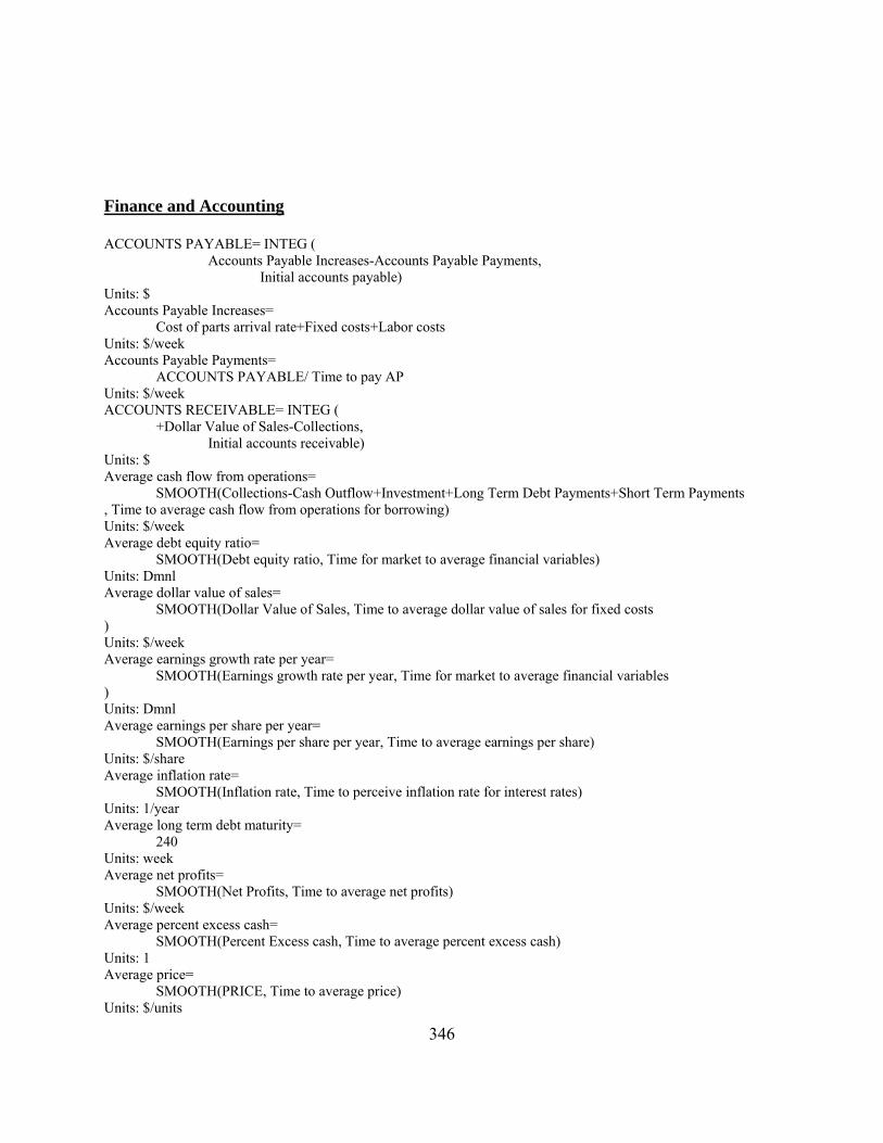
346
Finance and Accounting ACCOUNTS PAYABLE= INTEG ( Accounts Payable Increases-Accounts Payable Payments, Initial accounts payable) Units: $ Accounts Payable Increases= Cost of parts arrival rate+Fixed costs+Labor costs Units: $/week Accounts Payable Payments= ACCOUNTS PAYABLE/ Time to pay AP Units: $/week ACCOUNTS RECEIVABLE= INTEG ( +Dollar Value of Sales-Collections, Initial accounts receivable) Units: $ Average cash flow from operations= SMOOTH(Collections-Cash Outflow+Investment+Long Term Debt Payments+Short Term Payments , Time to average cash flow from operations for borrowing) Units: $/week Average debt equity ratio= SMOOTH(Debt equity ratio, Time for market to average financial variables) Units: Dmnl Average dollar value of sales= SMOOTH(Dollar Value of Sales, Time to average dollar value of sales for fixed costs ) Units: $/week Average earnings growth rate per year= SMOOTH(Earnings growth rate per year, Time for market to average financial variables ) Units: Dmnl Average earnings per share per year= SMOOTH(Earnings per share per year, Time to average earnings per share) Units: $/share Average inflation rate= SMOOTH(Inflation rate, Time to perceive inflation rate for interest rates) Units: 1/year Average long term debt maturity= 240 Units: week Average net profits= SMOOTH(Net Profits, Time to average net profits) Units: $/week Average percent excess cash= SMOOTH(Percent Excess cash, Time to average percent excess cash) Units: 1 Average price= SMOOTH(PRICE, Time to average price) Units: $/units

347
Average retained earnings= SMOOTH(Retained Earnings, Time to average retained earnings) Units: $/week Average return on equity per year= SMOOTH(Return on equity per year, Time for market to average financial variables ) Units: Dmnl Average salary per month= Average salary per month initial Units: $/Persons Base price= 35 Units: $/units CASH= INTEG ( Cash Inflow-Cash Outflow, Initial cash) Units: $ Cash Inflow= Collections+Equity Issuing+Long Term Borrowing+Short Term Borrowing Units: $/week Cash Outflow= Accounts Payable Payments+DIVIDENDS+Interest payments+Investment+Long Term Debt Payments +Short Term Payments+Taxes Units: $/week Change in Dividend Payout Ratio= (Indicated dividend payout ratio-DIVIDEND PAYOUT RATIO)/Time to adjust dividend payout ratio Units: 1/week Change in Dividends= (Indicated dividends-DIVIDENDS)/Time to adjust dividends Units: $/(Month*Month) Collections= ACCOUNTS RECEIVABLE/Time to collect accounts receivable Units: $/week Committed debt= Total liability+CAPITAL EQUIPMENT ON ORDER*Cost per unit of capital equipment per week Units: $ Committed debt adjusted for equity= MAX(0,Committed debt-Time to acquire capital equipment*Average cash flow from operations ) Units: $ Committed debt projected equity ratio= Committed debt adjusted for equity/Projected equity Units: Dmnl Cost of labor turnover= Average salary per month initial*(Labor Hiring Rate+Labor Firing Rate) Units: $/week Cost of material shipped= Cost of unit in finished inventory*Shipping Rate Units: $/week Cost of parts arrival rate= Unit cost of parts*Parts Arrival Rate

348
Units: $/week Cost of parts inventory= Unit cost of parts Units: $/units Cost of unit in finished inventory= Unit cost of parts+Value added in process Units: $/units Cost of WIP= 0.5*Cost of unit in finished inventory+0.5*Unit cost of parts Units: $/units Current assets= MAX(ACCOUNTS RECEIVABLE+CASH+Dollar value of inventory,0) Units: $ Current liabilities= ACCOUNTS PAYABLE+SHORT TERM DEBT Units: $ Current ratio= Current assets/Current liabilities Units: Dmnl Current ratio initial= 2.5 Units: Dmnl Debt equity ratio= Total liability/EQUITY Units: Dmnl Desired cash= Desired days dollar value of sales as cash*Dollar Value of Sales Units: $ DIVIDEND PAYOUT RATIO= INTEG ( Change in Dividend Payout Ratio, Indicated dividend payout ratio) Units: 1 DIVIDENDS= INTEG ( Change in Dividends, Initial dividends) Units: $/week Dollar value of inventory= (Cost of unit in finished inventory*FINISHED GOODS INVENTORY+Cost of parts inventory *PARTS INVENTORY+Cost of WIP*The WIP Inventory ) Units: $ Dollar Value of Sales= Shipping Rate*PRICE Units: $/week Earnings per share per year= Year length*Net Profits/SHARES Units: $/share Effect of cash conditions on dividends payments= WITH LOOKUP ( Average percent excess cash, ([(-1,0)-(1,2)],(-1,0),(-0.7,0.1),(-0.5,0.7),(-0.4,0.9),(-0.2,1),(0,1),(0.2 ,1),(0.4,1.1),(0.6,1.2),(1,1.3) )) Units: Dmnl

349
Effect of cash conditions on LTD payments= WITH LOOKUP ( Average percent excess cash, ([(-0.6,0)-(3,2)],(-0.5,0.7),(0,0.9),(0.5,1),(1,1.05),(1.5,1.15),(2,1.25) ,(2.5,1.35),(3,1.5) )) Units: Dmnl Effect of cash conditions on STD payments= Indicated change in cash Units: $/week Effect of cash constraints on hiring= WITH LOOKUP ( Average percent excess cash, ([(-1,0)-(0,1)],(-1,0),(-0.8,0),(-0.6,0.1),(-0.4,0.2),(-0.2,0.5),(0,1),(10 ,1) )) Units: Dmnl Effect of cash constraints on parts ordering= WITH LOOKUP ( Average percent excess cash, ([(-1,0)-(0,1)],(-1,0.9),(-0.8,0.97),(-0.6,0.98),(-0.4,0.99),(-0.2,1),(0, 1),(10,1) )) Units: Dmnl Effect of current ratio on short term borrowing= WITH LOOKUP ( Current ratio, ([(0,0)-(2,1)],(0,0),(0.5,0.4),(1,0.7),(1.5,0.9),(2,1),(2.5,1),(3,1),(5,1 ),(10,1),(20,1) )) Units: Dmnl Effect of debt equity ratio on capacity expansion= WITH LOOKUP ( Perceived debt equity ratio for capacity, ([(0,0)-(4,1)],(0,1),(0.25,1),(0.5,1),(0.75,1),(1,1),(1.25,0.9),(1.5,0.8) ,(1.75,0.5),(2,0.2),(2.25,0.1),(2.5,0),(2.75, 0),(3,0),(3.25,0),(3.5,0),(3.75,0),(4,0),(10,0) )) Units: Dmnl Effect of debt equity ratio on price= WITH LOOKUP ( Perceived debt equity ratio for capacity, ([(0,1)-(4,1.4)],(0,1),(0.25,1),(0.5,1),(0.75,1),(1,1),(1.25,1.02),(1.48012 ,1.03684),(1.75,1.06),(2,1.08),(2.25,1.1),( 2.5,1.125),(2.75,1.16),(3,1.2),(3.25,1.25),(3.5,1.3),(3.75,1.35),(4,1.4) )) Units: Dmnl Effect of debt equity ratio on short term borrowing= WITH LOOKUP ( Debt equity ratio, ([(0,0)-(4,1)],(0,1),(0.25,1),(0.5,1),(0.75,1),(1,1),(1.25,0.95),(1.5,0.9 ),(1.75,0.8),(2,0.7),(2.25,0.5),(2.5,0.3),(2.75 ,0.2),(3,0.1),(3.25,0.05),(3.5,0),(3.75,0),(4,0),(10,0) )) Units: Dmnl Effect of debt equity ratio on stock price= WITH LOOKUP ( Average debt equity ratio, ([(0,0.6)-(4,1)],(0,0.9),(0.5,0.95),(1,1),(1.5,0.95),(2,0.9),(2.5,0.85),( 3,0.8),(3.5,0.75),(4,0.7) )) Units: Dmnl Effect of delivery delay on market share= WITH LOOKUP ( Delivery delay quoted by company/Adjustment, ([(0,0)-(10,2)],(0,0),(0,0),(0,0),(0,1),(1,1),(1.5,1),(2,1),(2.5,1),(3,0.97 ),(4,0.95),(6,0.9),(8,0.75),(10,0.6),(20,0.1) )) Units: Dmnl

350
Effect of earning growth rate on stock price= WITH LOOKUP ( Average earnings growth rate per year, ([(-0.8,0)-(0.8,2)],(-0.5,0.5),(-0.4,0.6),(-0.3,0.7),(-0.2,0.8),(-0.1,0.9 ),(0,1),(0.1,1.1),(0.2,1.2),(0.3,1.25),(0.4,1.275),(0.5,1.3),(0.6,1.3),(0.7 ,1.3) )) Units: Dmnl Effect of price on market share= WITH LOOKUP ( Price acted on by customers/Competitor price, ([(0,0.8)-(6,1.2)],(0.75,1.1),(0.85,1.09),(0.9,1),(1,1),(2,1),(3,1),(4,0.99 ),(5,0.97),(6,0.9) )) Units: Dmnl Effect of return on equity on stock price= WITH LOOKUP ( Average return on equity per year, ([(0,0)-(0.6,6)],(0,0.1),(0.0495413,0.631579),(0.102752,1.13158),(0.157798 ,1.76316),(0.2,2.25),(0.255046,2.92105),(0.3,3.5),(0.35,4.25),(0.4,5),(0.45 ,6) )) Units: Dmnl EQUITY= INTEG ( Retained Earnings+Equity Issuing, Initial equity) Units: $ Equity Issuing = A FUNCTION OF( Indicated long term financing,Percent debt financing ) Equity Issuing= IF THEN ELSE(Customer Order Rate <2500, 0, Indicated long term financing* (1-Percent debt financing)) Units: $/week Gross profits= Dollar Value of Sales-Cost of material shipped-Fixed costs-Depreciation-Interest payments Units: $/week Indicated dividend payout ratio= Payout ratio indicated by return on equity*Effect of cash conditions on dividends payments Units: 1 Indicated long term financing= MAX(0,Investment+Long Term Debt Payments-Average cash flow from operations ) Units: $/week Inflation rate initial= 0 Units: 1/year Initial accounts payable= Accounts Payable Increases*Time to pay AP Units: $ Initial accounts receivable= Dollar Value of Sales*Time to collect accounts receivable Units: $ Initial cash= INITIAL(Desired cash) Units: $ Initial equity= Total assets/(1+Debt equity ratio initial) Units: $

351
Initial long term debt= (Debt equity ratio initial*EQUITY-Current liabilities) Units: $ Initial shares= 3e+006 Units: share Initial short term debt= MAX(0,(Current assets/Current ratio initial)-ACCOUNTS PAYABLE) Units: $ Interest payments= Interest rate*(LONG TERM DEBT+SHORT TERM DEBT)/48 Units: $/week Investment= Capital Equipment Arrivals*Cost per unit of capital equipment per week Units: $/week LONG TERM DEBT= INTEG ( +Long Term Borrowing-Long Term Debt Payments, 0) Units: $ Long Term Debt Payments= (LONG TERM DEBT/Average long term debt maturity)*Effect of cash conditions on LTD payments Units: $/week Net Profits= Gross profits-Taxes Units: $/week Percent debt financing= WITH LOOKUP ( Debt equity ratio, ([(0,0)-(2,1)],(0,1),(0.25,1),(0.5,0.9),(0.75,0.5),(1,0.1),(1.25,0),(1.5, 0),(1.75,0),(2,0) )) Units: 1 Percent Excess cash= IF THEN ELSE(Desired cash>0, (CASH-Desired cash)/Desired cash, 0) Units: 1 Price earning ratio per year= Price earning ratio normal*Effect of return on equity on stock price*Effect of earning growth rate on stock price *Effect of debt equity ratio on stock price Units: $/$ Profit= SMOOTH( Net Profits, 4) Units: $ Projected equity= EQUITY+Time to acquire capital equipment*Average retained earnings Units: $ Retained Earnings= MAX(0,Net Profits-DIVIDENDS) Units: $/week Return on equity per year= Year length*Net Profits/EQUITY Units: Dmnl Return on Investment= Net Profits/Investment

352
Units: Dmnl Risk free interest rate= 0.02 Units: 1/year Risk premium of debt= WITH LOOKUP ( Debt equity ratio, ([(0,0)-(4,0.08)],(0,0.015),(0.5,0.0175),(1,0.02),(1.5,0.0225),(2,0.025), (2.5,0.03),(3,0.04),(3.5,0.055),(4,0.075) )) Units: 1/year SHARES= INTEG ( (Equity Issuing/STOCK PRICE), Initial shares) Units: share Short Term Borrowing= MAX(0,Indicated change in cash)*Effect of current ratio on short term borrowing *Effect of debt equity ratio on short term borrowing Units: $/week SHORT TERM DEBT= INTEG ( +Short Term Borrowing-Short Term Payments, 1000000) Units: $ Short Term Payments= Indicated short term payments*Effect of short term debt on payments+0*SHORT TERM DEBT / (Time to pay STD) Units: $/week Taxes= IF THEN ELSE(Gross profits>0, Gross profits*Tax rate, 0) Units: $/week Total assets= BOOK VALUE OF FIXED ASSETS+Current assets Units: $ Total liability= Current liabilities+LONG TERM DEBT Units: $ Value added in process= Running costs of tools+Labor costs/Average production completions Units: $/units

353
APPENDIX B: 2-SAMPLE T-TEST RESULTS FOR THE DIFFERENCE BETWEEN MEANS FOR THE RESUMPTION ALGORISM

354
B-1: t-test results for the mean production rate - PREF module Two-sample T for Non Segmented PREF vs Segmented PREF N Mean StDev SE Mean Non Segmented 50 1796 215 31 Segmented 50 1816 242 35 Difference = mu Non Segmented PREF - mu Segmented PREF Estimate for difference: -20.4 95% CI for difference: (-113.0, 72.3) T-Test of difference = 0 (vs not =): T-Value = -0.44 P-Value = 0.663 DF = 92
SegmenteNon Segm
2400
2200
2000
1800
1600
1400
1200
1000
Boxplots of Non Segm and Segmente(means are indicated by solid circles)
Non Segm Segmente
1400
1900
2400
Dotplots of Non Segm and Segmente(means are indicated by lines)

355
B-2: t-test results for the mean production rate - PRES module Two-sample T for Non Segmented PRES vs Segmented PRES N Mean StDev SE Mean Non Segm 50 1248.9 52.8 7.5 Segmente 50 1254.1 71.6 10 Difference = mu Non Segmented PRES - mu Segmented PRES Estimate for difference: -5.2 95% CI for difference: (-30.2, 19.8) T-Test of difference = 0 (vs not =): T-Value = -0.41 P-Value = 0.679 DF = 90
Non Segm Segmente
1000
1100
1200
1300
1400
Boxplots of Non Segm and Segmente(means are indicated by solid circles)
Non Segm Segmente
1000
1100
1200
1300
1400
Dotplots of Non Segm and Segmente(means are indicated by lines)
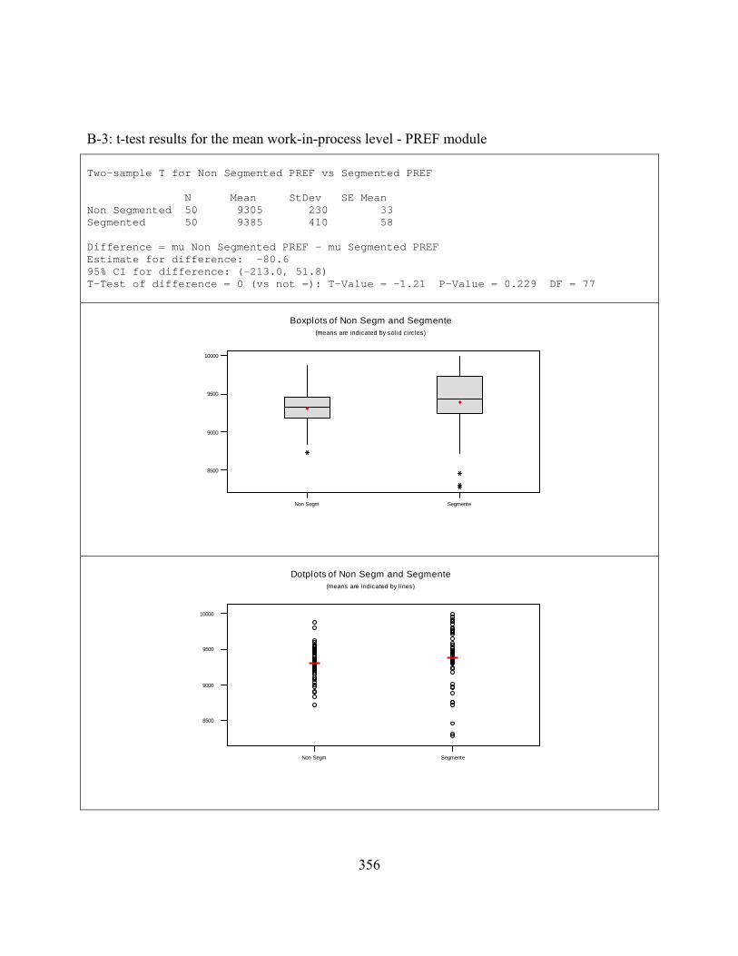
356
B-3: t-test results for the mean work-in-process level - PREF module Two-sample T for Non Segmented PREF vs Segmented PREF N Mean StDev SE Mean Non Segmented 50 9305 230 33 Segmented 50 9385 410 58 Difference = mu Non Segmented PREF - mu Segmented PREF Estimate for difference: -80.6 95% CI for difference: (-213.0, 51.8) T-Test of difference = 0 (vs not =): T-Value = -1.21 P-Value = 0.229 DF = 77
Non Segm Segmente
8500
9000
9500
10000
Boxplots of Non Segm and Segmente(means are indicated by solid circles)
Non Segm Segmente
8500
9000
9500
10000
Dotplots of Non Segm and Segmente(means are indicated by lines)
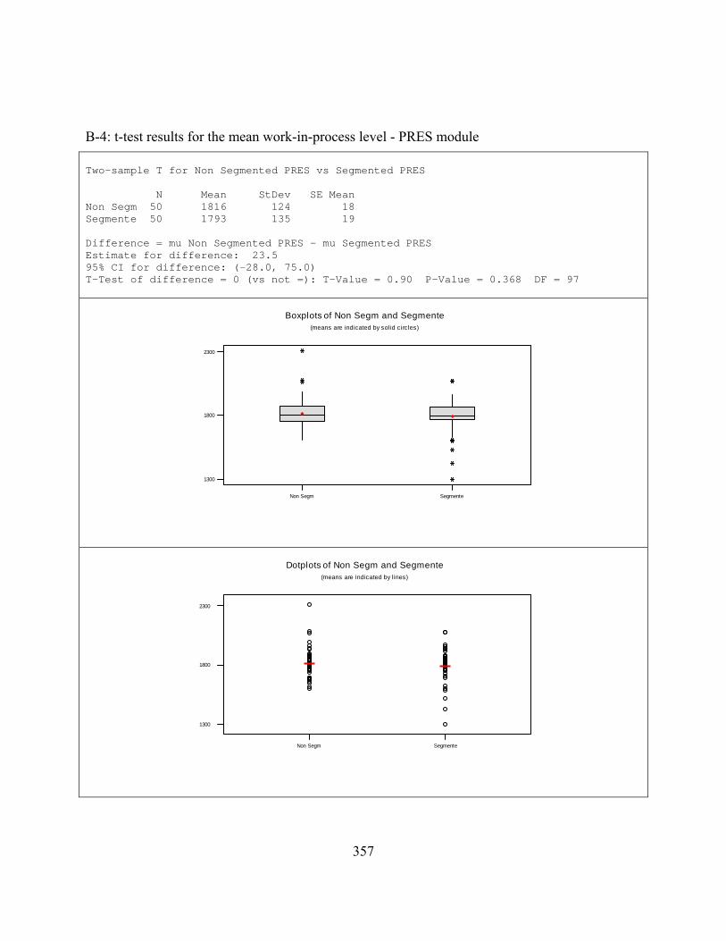
357
B-4: t-test results for the mean work-in-process level - PRES module Two-sample T for Non Segmented PRES vs Segmented PRES N Mean StDev SE Mean Non Segm 50 1816 124 18 Segmente 50 1793 135 19 Difference = mu Non Segmented PRES - mu Segmented PRES Estimate for difference: 23.5 95% CI for difference: (-28.0, 75.0) T-Test of difference = 0 (vs not =): T-Value = 0.90 P-Value = 0.368 DF = 97
SegmenteNon Segm
2300
1800
1300
Boxplots of Non Segm and Segmente(means are indicated by solid circles)
SegmenteNon Segm
2300
1800
1300
Dotplots of Non Segm and Segmente(means are indicated by lines)

358
LIST OF REFERENCES
Adamides E. (2006). A system dynamics computer-based learning environment for the formulation of manufacturing strategy. 25th International Conference of the System Dynamics Society, July 23-27, Nijmegen, The Netherlands
Aguilar-Saven, R. S. (2004). Business process modeling: Review and framework. International Journal of Production Economics, 90(2), 129-149
Alexopoulos, C. (2006). Statistical estimation in computer simulation. Chapter 8 in Henderson, S. and Nelson, B.; Eds. Handbooks in Operations Research and Management Science, Vol. 13: Simulation. North-Holland Elsevier, The Netherlands
Alur, R., Henzinger, T., Lafferriere, G., Pappas, G., (2000). Discrete abstraction of hybrid systems. IEEE, 88(7), 971-984
An, L., Jehn, J. (2005). On developing system dynamics model for business process simulation. The Winter Simulation Conference WSC’05, Dec 5-8, Orlando FL
Anthony, N. (1965). Planning and control systems: a framework for analysis. 9th printing at 1977, Division of Research at the Graduate School of Business Administration, Harvard University, Boston, MA
Anthony, R. (1988). The management control functions. Harvard Business School Press, Boston, MA
Anthony, R., Dearden, J., Bedford, N. (1989). Management Control Systems. 6th Ed., IRWIN, IL
Anthony, N., Govindarajan, G. (1998). Management control systems. 9th Ed. Irwin McGraw-Hill
Ashayeri, J., Keij R., Broker, A. (1998). Global business process re-engineering: a system dynamics-based approach. International Journal of Operations and Production Management, 18 (9/10), 817-831
Aull-Hyde, R., Erdogan, S., Duke, J. (2006). An experiment on the consistency of aggregated comparison matrices in AHP. European Journal of Operational Research, (171), 290–295
Aytug, H., Lawley, M., McKay, K., Mohan, S., Uzsoy, R. (2005). Executing production schedules in the face of uncertainty: A review and some future directions. European

359
Journal of Operational Research, (161), 86-110
Babat, V., Sturrock, D. (2003). The Arena product family: Enterprise modeling solutions. The Winter Simulation Conference WSC’03, Dec 7-10, New Orleans, USA
Baines, T., Harrison, D. (1999). An opportunity for system dynamics in manufacturing system modeling. Production Planning and Control, 10(6), 542-552
Banks, J., Carson II, J., Nelson, B., Nicol, D. (2005). Discrete event System Simulation. Perntice-Hall, NJ, USA
Barton, J., Love, D., Taylor, G. (2001). Evaluating design implementation strategies using simulation. International Journal of Production Economics, (72), 285-299
Baudin; M. (1990). Manufacturing systems analysis. YOURDON PRESS; Prentice Hall, NJ
Bauer; C., Whitehouse; G., Brooks; G. (1982). Computer simulation of production system: Phase I, Technical Report: COE No. 82-83-1, The university of Central Florida, Orlando
Bezemer, J., Akkermans, H. (2003). Not with a bang, but with a whimper: Understanding delays in semiconductor supply chain dynamics. 21st International Conference of the System Dynamics Society, July 20-24, New York, USA
Bodoh, D., Wieland, F. (2003). Performance Experiments with the high level architecture and the total airport and airspace model (TAAM). 17th Workshop on Parallel and Distributed Simulation, IEEE, San Diego, CA, June 10-13, 31-39
Boer, C., Bruin, A., Verbraeck, A. (2006a). Distributed Simulation in industry – A survey, Part 1 – the COTS vendors. The Winter Simulation Conference WSC’06, Dec 3-6, Monterey CA, 1053-1060
Boer, C., Bruin, A., Verbraeck, A. (2006b). Distributed Simulation in industry – A survey, Part 2 – Experts on distributed simulation. The Winter Simulation Conference WSC’06, Dec 3-6, Monterey CA, 1061-1068
Bonder, D., McGinnis, L. (2002). A structured approach to simulation modeling of manufacturing systems. IIE’s IERC, May 19-21, Orlando FL
Borshchev, A. (2001). AnyLogic 4.0: Simulating hybrid systems with extended UML-RT. Simulation News Europe, 31, 1-2
Borshchev, A., Filippov, A. (2004). From system dynamics and discrete event to practical agent based modeling: reasons, techniques, tools. 22nd International Conference of the System Dynamics Society, July 25 - 29, Oxford, England

360
Borshchev, A., Karpov, Y., Kharitonov, V. (2002). Distributed Simulation of Hybrid Systems with AnyLogic and HLA. Future Generation Computer Systems, 18(6)
Borshchev, A, Kolesov, Y., Senichenkov, Y. (2000). Java engine for UML based hybrid state machines. The Winter Simulation Conference WSC’00, Orlando, FL, 1888-1894
Bononi, L., D’angelo, G., Donatello, L. (2003). HLA-based adaptive distributed simulation of wireless mobile systems. 17th Workshop on Parallel and Distributed Simulation, IEEE, San Diego, CA, June 10-13, 40-49
Botta-Genoulaz, V., Millet, P., Grabort, B. (2005). A survey on the recent research literature on ERP systems. Computers in Industry, 56, 510-522.
Bradl, P. (2003). The use of SD in management: reasons and applications. 21st International Conference of the System Dynamics Society, July 20-24, New York, USA
Brennen, R. (2000). A simulation test bed to evaluate multi-agent control of manufacturing systems. The Winter Simulation Conference, WSC’00, Dec 10-13, Orlando, FL
Bryant, R. (1977). Simulation of packet communication architecture computer systems. Computer Science Laboratory, MIT, Cambridge, MA
Bouchhima, F., Nicolescu, G., Aboulhamid, E., Abid, M. (2005). Discrete-Continuous Simulation Model for Accurate Validation in Component-Based Heterogeneous SoC Design. IEEE International Workshop on Rapid System Prototyping 2005, 181-187
Carrie; A. (1988). Simulation of manufacturing systems. John Wiley & Sons, GB.
Chandy, k., Misra, J. (1978). Distributed simulation: A case study in the design and verification of distributed programs. IEEE Transactions on Software Engineering, 5(5), 440-452
Chang, Y., Makatsoris, H. (2001). Supply chain modeling using simulation. International Journal of Simulation, 2(1), 24-30
Chatha, K., Weston, R. (2005). Combined enterprise and simulation modeling in support of process engineering. International Journal of Computer integrated manufacturing. 18(8), 652-670
Cho, H., Son, T., Jones, A. (2006). Design and conceptual development of shop-floor controllers through the manipulation of process plans. International Journal of Computer Integrated Manufacturing. 19(4), 359-376
Choi K, Bae D, Kim T. (2005). DEVS-based software process simulation modeling: formally specified, modularized, and extensible SPSM. The International Workshop on Software

361
Process Modeling and Simulation (ProSim ‘05), St. Louis, MO.
Choi, K.; Bae, D., Kim, T. (2006). An approach to a hybrid software process simulation using the DEVS formalism. Software Process: Improvement and Practice, 11(4), 373-383
Chouikha, M., Decknatel, G., Darth, R., Frey, G., Muller, C., Simon, C., Thieme, J., Wolter, K. (2000). Petri net-based descriptions of discrete-continuous systems. Automatisierungstechnik, 48 (9), Oldenbourg Verlag, Germany
Cowling, P., Johansson, M. (2002). Using real time information for effective dynamic scheduling. European Journal of Operational Research, (139), 230-244
Dai, J., Zhu, F., Ma, X. (1996). Computer integrated hybrid modeling support systems for enterprise decisions making. IEEE International Conference on Systems, Management, and Cybernetics, Oct 14-17, Vol. 2, 947-952
Davenport, T. (1998). Putting the enterprise into the enterprise system. Harvard Business Review, July/Aug 1998, 121-131.
Davenport, T. (2000). Mission critical: realizing the promise of enterprise systems. Harvard Business School Press, Boston, MA.
De Souza, R., Huynh, R., Chandrashekar, M., Thevenard, D. (1996). A comparison of modeling paradigms for manufacturing line. IEEE International Conference on Systems, Management, and Cybernetics, Oct 14-17, Beijing, China, 1253-1258
Dillard, J., Yuthas, K. (2006). Enterprise resource planning systems and communicative actions. Critical Perspectives on Accounting. (17) 202-223
Donzelli, P., Iazeolla, G. (1996). Performance modeling of the software development processes. The 8th Simulation Symposium, Genova, Italy, Oct. 24-26
Ehrahardt, N., Brigham, E. (2003), Corporate finance; a focused approach. THMOSON South-Western, USA
Eskandari, H., Rabelo, L. (2006). Handling uncertainties in the analytic hierarchy process: a stochastic approach. International Journal of Information Technology and Decision Making, (5)3
Filippov, A., Borshchev, A. (2001). Modeling S-class car seat control with AnyLogic, 2001 OMER-2: Object-Oriented Modeling of Embedded Real-Time Systems, GI- Workshops, pp 46-50, Herrsching am Amersee, Germany
Forman, E., Peniwati, K. (1998). Aggregating individual judgments and priorities with the

362
analytic hierarchy process. European Journal of Operational Research, (108) 65–169
Forrester, J. (1965). Industrial Dynamics. MIT Press, 4th Ed., MA, USA
Forrester, J. (1968). Market growth as influenced by capital investment. Industrial Management Review (currently Sloan Management Review) 9(2), Winter 1968, 83-105
Forrester, J. (1973). World Dynamics. Productivity Press, USA
Forrester, J. (1975). Industrial dynamics after the first decade. Chapter 8 in “Collected papers of Jay W. Forrester”, Wright-Allen Press, Inc.
Forrester, J. (1991). System dynamics and lessons of 35 years. Sloan School of Management, Document # D-4224-4, Online at www.sysdyn.clexchange.org/sdep/papers/D-4224-4.pdf
Fishwick, P. (1995). Simulation Model Design and Execution. Prentice-Hall, USA
Fowler, J., Rose, O. (2004). Grand Challenges in Modeling and Simulation of Complex Manufacturing Systems. Simulation, 80(9) 469-476
Fox, M., Gurninger, M. (1998). Enterprise modeling. AI Magazine, 19(3), 109-121
Frey, P., Carter, H., Wilsey, P. (1997). Parallel synchronization of continuous time discrete event simulators. ICPP; the IEEE international Conference on Parallel Processing, Aug 11-15, Washington DC, pp 227-231
Fujii, S., Tsunoda, H., Ogita, A., Kidani, Y. (1994). Distributed simulation model for computer integrated manufacturing. The WSC’94, Dec 5–8, Orlando, FL, pp 946 - 953
Fujii, S., Ogita, A., Kidani, Y., Kaihara, T. (1999). Synchronization mechanisms for integration of distributed manufacturing systems. Simulation, 72(3), pp 187-197
Fujii, S., Kaihara, T., Morita, H. (2000). A distributed virtual factory in agile manufacturing environment. International Journal Production Research. 38(17), 4113-4128
Fujii, S., Morita, H., Tanaka, T. (2000). A basic study on autonomous characterization of square array machining cells for agile manufacturing”. The WSC’02, Dec, Orlando, FL, pp 1282 - 1289
Fujimoto, R. (2000). Parallel and distributed simulation systems. John Wiley & Sons Inc. USA
Fujimoto, R. (2001). Parallel and distributed simulation systems. The WSC'01. Peters, B., Smith, J., Medeiros, D., Rohrer, M. (Eds.), 147-157.
Gheorghe, L., Bouchhima, F., Nicolescu, G., Boucheneb, H. (2006). Formal definitions of

363
simulation interfaces in a continuous/discrete co-simulation. The 17th IEEE International. Workshop on Rabid System Prototyping
Giambiasi, N., Paillet, J., Chane, F. (2003). From Timed Automata to DEVS models. The WSC’03, Dec 5-7, New Orleans, LA
Godding, G., Sarjoughian, H., Kempf, K. (2003). Semiconductor supply network simulation. The WSC,03, Dec 03, New Orleans, LA
Greene, J. (1997). Production and inventory control handbook. 3rd Ed., McGraw-Hill, USA
Gregoriades, A., Karakostas, B. (2003). Unifying business objects and systems dynamics as a paradigm for developing decision support systems. Decision Support Systems (1049), pp 1-5
Größler, A., Stotz, M., Schieritz, N. (2003). A software interface between system dynamics and agent-based simulations – Linking Vensim and RePast. The 21st System Dynamics Society International Conference, July 20-24, New York, USA
Gu, Z., Shin, K. (2004). Synthesis of real time implementation from UML-RT models. 2nd RATS Workshop on model-driven embedded systems, MoDES’04, Toronto, Canada, May 25-28
Haler, D. (1987). Statecharts: A visual formalism for complex systems. Science of Computer Programming (8), 231-274
Hannet, J. (1999). From the aggregate plan to lot-sizing in multi-level production planning”, in Brandimarte, P., and Villa, A. (Eds.) Modeling Manufacturing Systems from aggregate planning to real time control. Springer-Verlag Berlin, Germany
Helal, M., Rabelo, L., (2004). An enterprise simulation approach to the development of dynamic balanced scorecards. ASEM’04; The American Society of Engineering Management Conference, Oct 20-23, Alexandria, Virginia
Hermsillo Worley, J., Chata, K., Weston, R., Aguirre, O., Garbot, B. (2005). Implementation and optimization of ERP systems: a better integration of processes, roles, knowledge and user competencies. Computers in Industry, (56), pp 620-638.
Hitomi, K. (1996). Manufacturing systems engineering. 2nd Ed., Taylor and Francis, Great Britain
Huang, G., Lau, J,. Mak, K. (2003). The impact of sharing production information on supply chain dynamics: a review of the literature. International Journal of Production Research, 41(7), 1483-1517

364
Jacobson, I., Booch, G., Rumbaugh, J. (2001). The unified software development process. Addison-wesley, USA
Jarke, M., Jeusfeld, M., Peters, P., Pohl, K. (1997). Coordinating distributed organizational knowledge. Data & Knowledge Engineering, (23), 247-268
Jefferson, D. (1985). Virtual Time. The ACM Transactions on Programming Languages and Systems. 7(3), 404-425.
Johnson, S., Eberlein, B. (2002). Alternative modeling approaches: a case study in the gas and oil industry. The 2002 System Dynamics Society International Conference, July 27-30, Palermo, Italy
Jones, A., Yih, Y., Wallace, E. (2001) Mentoring and controlling operations. Chapter 65 in The Handbook of Industrial Engineering: technology and operations management, Gavriel Salvendy (Ed.), Wiley, NY
Kaplan, R, Norton, D. (1996). The balanced scorecard: Translating strategy into action. Harvard Business School Press, Boston, MA.
Kaplan, R., Norton, D. (2001). The strategy focused organization. Harvard Business School Press, Boston, MA.
Keenan, P., Paich, M. (2004). Modeling General Motors and North American automobile market. The 22nd International Conference of the System Dynamics Society, July 25 - 29, 2004, Oxford, England
Kelton, W., Sadowski, R., and Sadowski, D. (2002). Simulation with Arena. McGrawHill, USA
Kosturiak, J., Gregor, M. (1999). Simulation in production system life cycle. Computers in Industry, (38), 159-172
Kowalewski, S., Stursberg, M., Fritz, M., Graf, M., Hoffmann, I, Preubig, J, Remelhe, P., Simon, S., Treseler, H. (1999). A case study in tool-aided analysis of discretely controlled continuous systems: The two tanks problem”, in Antsaklis, P. et al. (Eds.): Hybrid Systems V, Springer-Verlag Berlin Heidelberg, pp 163-185
Kuhl, F., Weatherly, R., Dahmann, J. (2000). Creating computer simulation systems: an introduction to the high level architecture. Prentice Hall PTR, NJ, USA
Larson, K. (1997). Essentials of Financial Accounting. Irwin McGraw-Hill, USA
Lavoie, P., Kenne, J., Gharbi, A. (2007). Production control and combined discrete continuous simulation in a failure prone transfer lines. International Journal of Production Research

365
(45) 24, 5667 - 5685
Law, A., Kelton, W. (2000). Simulation modeling and analysis. McGrawHill, USA
Lee, Y., Cho, M., Kim, S., Kim, Y. (2002a). Supply chain simulation with discrete-continuous combined modeling. Computer and Industrial Engineering, (43), 375-392
Lee, J., Hsu, P. (2002). UML-based modeling and multi-threaded simulation for hybrid systems. The 2002 IEEE Int. Conf. on Control Applications, Sept 18-20, Glasgow, Scotland
Lee, S., Ramakrishnan, S., Wysk, R. (2002b). A federation coordinator for simulation based control and analysis. The WSC’02, Orlando, FL, 1986-1994
Lee, S., Wysk, R. (2004). A resource reconciliation mechanism for a manufacturing federation coordinated using MRP/ERP system. The WSC’04, pp 30-38
Lee, J.; Zhou, M.; Hsu, P. (2004). A multi-paradigm modeling approach for hybrid dynamic systems. IEEE Intl. Symposium on Computer Aided Control System design, Taipie, Tiwan, Sept 2-4, pp 77-82
Lendermann, P. (2006). About the need for distributed simulation technology for the resolution of real-world manufacturing and logistics problems. WSC’06: Dec 3-6, Monterey CA, pp 1119-1128
Lertpattarapong, C. (2002). Applying system dynamics approach to the supply chain management problem. A Master thesis, MIT
Levin, T., Levin, I. (2002). Hybrid systems modeling in learning science and technology. Journal of Computers in Mathematics and Science Teaching. 21(4), 313-330
Levin, T., Levin, I. (2003). Integrating hybrid modeling with system dynamics. The 21st International Conference, System Dynamics Society, July 20-24, NY, USA
Lin, C., Baines, T., O’Kane, J, Link, D. (1998). A generic methodology that aids the application of system dynamics to manufacturing system modeling. International Conf. on Simulation. Sept 30 – Oct 2 (IEEE Conf Publ. No. 457)
Love, D., Barton, J. (1996). Evaluation of design decisions through CIM and simulation. Integrated manufacturing systems, 7(4), 3-11
Lyneis, J. (1980). Corporate planning and policy design: A system dynamics approach. The MIT Press, Cambridge, MA, USA
Ma, Q., Judd, R., Lipset, R. (2001). Distributed manufacturing simulation environment. The

366
Summer Computer Simulation Conf., July 15-17, Orlando, FL
Maler, O., Manna, Z., Pnueli, A. (1992). From timed to hybrid systems. In Real-Time: Theory in Practice, Eds. Bakker, J.; Huizing, C.; Roever, W.; Rozenberg, G.; Springer-Verlag, Germany
Mandal, P., Sohal, A. (1998). Modeling helps in understanding policy alternatives: A case. Journal of Management in Engineering, Jan/Feb , pp 41-48
Martin, R. (2001). A hybrid model of the software development process. PhD Thesis, Portland State University
Morecroft, J., (1985). Rationality of the analysis of behavior simulation models. Management Science, 31( 7), 900-916
Morecroft, J., Robinson, S. (2007). Explaining puzzling dynamics: comparing the use of system dynamics and discrete event simulation. The 23rd International Conference, System Dynamics Society, July 17-21, MA, USA
Moustakis, V. (2000). Material requirements planning. Report produced for the EC funded project, Last accessed on Feb 2006: http://www.adi.pt/docs/innoregio_MRP-en.pdf
Pegden, C., Shannon, R., Sadowski, R. (1990). Introduction to simulation using SIMAN”, McGraw-hill, USA
Pepyne, D., Cassandras, C. (2000). Optimal control of hybrid manufacturing systems in manufacturing”, Proceedings of the IEEE. 88 (7), 1108-1123
Pfeiffer, A., Kadar, B., Monostori, L., Karnok, D. (2008). Simulation as one of the core technologies for digital enterprises: assessment of hybrid scheduling methods. International Journal of Computer Integrated Manufacturing. 21(2), 206-214
Pritsker, A, O’Reilly, J., LaVal, D. (1997). Simulation with Visual SLAM and AweSim”, John Wiley & Sons, USA
Popper, K. (1959). The logic of scientific discovery”, Basic Books, NY
Porter, M. (1985). Competitive advantage: creating and sustaining superior performance. The FREE PRESS, NY.
Pugh III, R. (1981). Introduction to system dynamics with DYNAMO. The MIT Press, MA
Rabelo, L.; Eskandari, H.; Shaalan, T.; Helal, M.; 2007, “Value Chain Analysis Using Hybrid Simulation and AHP” International Journal of Production Economics, V 105, # 2, pp

367
536-547
Rabelo, L., Helal, M., Son, Y., Jones, A., Min, J., Deshmukh, A. (2003). A hybrid approach to manufacturing enterprise simulation”, The WSC’03, Dec 7-10, New Orleans, LA
Rabelo, L., Helal, M., Jones, A., Min, H. (2005). Enterprise simulation: A hybrid system approach. International Journal of Computer Integrated Manufacturing. 18(6), 498-508
Rabelo, L., Speller, T., Burns, C., Meade, P. (2004). Analysis of sustaining growth in a corporation. In: Y. Hosni and T. Khalil, Editors, Management of Technology, Elsevier Ltd, San Diego, CA, pp. 545–556
Research on modeling and design of manufacturing systems, Cranfield University, UK, http://www.cranfield.ac.uk/sims/mem/mdms/aitoroyarbide/researchaitoroyarbide.html, since 2000, last seen Dec 2003
Reid, R., Koljonen, E. (1999). Validating a manufacturing paradigm: A SD modeling approach. The WSC’99, pp 759-765
Riezebos, J. (2004). Time bucket length and lot-splitting approach. International Journal of Production Research, 42(12), 2325-2338
Ritchie-Dunham, J., Morrice, D., Scott, J., Anderson, E. (2000). A strategic supply chain simulation model. The WSC’00, Dec 10-13, Orlando, FL
Saad, S., Perera, T., Wickramarachchi. (2003). Simulation of distributed manufacturing enterprise: a new approach. The WSC’03, Dec 5-8, New Orleans, LA
Shapiro, J. (2001). Modeling the supply chain. Duxbury, USA
Senge; P, Sterman; J. (1994). System thinking and organizational learning: acting locally and thinking globally in the organization of the future. in Morecroft; J., Sterman; J. (Eds.) “Modeling for Learning Organizations”, Productivity Press, Portland; OR.
Sinreich, D., Shints, B. (2006). A robust FMS control architecture with an embedded adaptive scheduling mechanism. Journal of Manufacturing Systems. 25(4), 301-312
Simchi-Levi, D.; Kaminsky, P.; Simchi, E. (2008), Designing and Managing the Supply Chain: Concepts, Strategies and Case Studies. McGraw-Hill Irwin, NY
Smith, J. (2003). Survey on the use of simulation for manufacturing system design and operation. Journal of Manufacturing Systems, 22(2); 157-171
Steinman, J. (1990). Multi-Node Test Bed: A Distributed Emulation of Space Communications for the Strategic Defense System. The 21st Annual Pittsburgh Conference on Modeling

368
and Simulation. 21(3), May, pp 1111-1115.
Steinman J. (1991). SPEEDES: Synchronous parallel environment for emulation and discrete event simulation. The SCS Western Multiconference on Advances in Parallel and Distributed Simulation, 23(1), 95-103.
Steinman, J. (1992). SPEEDES: A multiple-synchronization environment for parallel discrete-event simulation. International Journal in Computer Simulation. (2), 251-286.
Steinman, J. (1993). Breathing Time Warp. The 7th workshop on parallel and distributed simulation, San Diego, CA, May 16-19, pp 109 – 118
Steinman, J., Lee, C., Wilson, F., Nicol, D. (1995). Global Virtual Time and distributed synchronization. The 9th workshop on Parallel and distributed simulation, p.139-148, June 13-16, 1995, Lake Placid, NY
Steinman, J. (1996). Discrete-event simulation and the event horizon part 2: event list management. ACM SIGSIM Simulation Digest, 26(1), 170-178
Sterman, J. (1989). Modeling managerial behavior: misperception of feedback in a dynamic decision making experiment. Management Science. 35(3), pp 321-339
Sterman, J. (2000). Business dynamics: systems thinking and modeling for a complex world. McGraw Hill, New York, USA
Sterman, J., Repenning, N., Kofman, F. (1997). Unanticipated side effects of successful quality programs: Exploring a paradox of organizational improvement. Management Science. (43), 503-521
System Dynamics Society Web site at: http://www.albany.edu/cpr/sds/
Towill, D., Edghill, J. (1989). The use of system dynamics in manufacturing systems engineering. Transactions of the Institute of Measurement and Control, (11), 208-216
Umble, M., Srikanth; M. (1996). Synchronous manufacturing. The Spectrum Publishing Company, USA
Umeda, S., Zhang, F. (2008). Hybrid modeling approach for supply chain simulation. in IFIP International Federation for Information Processing, Tomasz Koch, Ed., Boston: Springer, pp 453-460
Venkateswarana, J., Son, Y. (2005). Hybrid system dynamics discrete event simulation based architecture for hierarchical production planning. International Journal Production Research. 43(20), 4397-4429

369
Ventana Systems Inc., Vensim User’s Guide, www.vensim.com
Vernadat, F. (2002). Enterprise modeling and integration (EMI): Current status and research perspectives. Annual Reviews in Control, (26), 15-25
Viswanadham; N. (2000). Analysis of manufacturing enterprise: An approach to leveraging value delivery processes for competitive advantage. Kluwer Academic Publishers, USA
Wakeland, W., Gallaher, E., Macovesky, L, Aktipis, C. (2004). A comparison of system dynamics and agent based simulations applied to the study of the cellular receptor dynamics. The 37th Annual Hawaii Intl. Conf. on System Sciences, 4-7 Jan
Welch, P. (1983). The statistical analysis of simulation results. In S. Lavenberg (Ed,) The Computer Performance Modeling Handbook, 268–328. New York: Academic Press.
Wiendahl, H, Breithaupt, J. (1998). Automatic production control: a new approach in production planning and control based on methods of control theory. Drexl, A., Kimms, A. (Eds.) Beyond manufacturing resource planning (MRP II), Springer, Berlin, Germany, 335–356.
Wu; B. (1992). Manufacturing system design and analysis. CHAPMAN & HALL, GB
Wu; B. (2002). Handbook of manufacturing and supply system design. aylor and Francis, London.
XJ-Technologies, (2008) AnyLogic User’s manual; www.xjtek.com
XJ-Technologies, (2008) AnyLogic: Technical Overview ; www.xjtek.com
Zeigler, B. (1976). Theory of modeling and simulation. Wiley, NY
Zeigler, B., Praehofer, P., Kim, T. (2000). Theory of modeling and simulation: Integrating discrete event and continuous complex dynamic systems”; 2nd Ed., Academic Press, USA
Zulch G., Jonsson U., Fischer J. (2002). Hierarchical simulation of complex production systems by coupling of model. International Journal of Production Economics. (77), 39-51
Recommended