A Framework for Parameterizing Eddy Potential Vorticity Fluxes
DAVID P. MARSHALL AND JAMES R. MADDISON
Department of Physics, University of Oxford, Oxford, United Kingdom
PAVEL S. BERLOFF
Department of Mathematics, Imperial College of Science, Technology and Medicine, London, United Kingdom
(Manuscript received 7 March 2011, in final form 20 October 2011)
ABSTRACT
A framework for parameterizing eddy potential vorticity fluxes is developed that is consistent with con-
servation of energy and momentum while retaining the symmetries of the original eddy flux. The framework
involves rewriting the residual-mean eddy force, or equivalently the eddy potential vorticity flux, as the di-
vergence of an eddy stress tensor. A norm of this tensor is bounded by the eddy energy, allowing the com-
ponents of the stress tensor to be rewritten in terms of the eddy energy and nondimensional parameters
describing the mean shape and orientation of the eddies. If a prognostic equation is solved for the eddy
energy, the remaining unknowns are nondimensional and bounded in magnitude by unity. Moreover, these
nondimensional geometric parameters have strong connections with classical stability theory. When applied
to the Eady problem, it is shown that the new framework preserves the functional form of the Eady growth
rate for linear instability. Moreover, in the limit in which Reynolds stresses are neglected, the framework
reduces to a Gent and McWilliams type of eddy closure where the eddy diffusivity can be interpreted as the
form proposed by Visbeck et al. Simulations of three-layer wind-driven gyres are used to diagnose the eddy
shape and orientations in fully developed geostrophic turbulence. These fields are found to have large-scale
structure that appears related to the structure of the mean flow. The eddy energy sets the magnitude of the
eddy stress tensor and hence the eddy potential vorticity fluxes. Possible extensions of the framework to
ensure potential vorticity is mixed on average are discussed.
1. Introduction
The ocean is populated by an intense geostrophic
eddy field with a dominant energy-containing scale on
the order of 100 km at midlatitudes. To obtain plausible
turbulent cascades of dynamic and passive tracers, it is
necessary for models to resolve spatial scales of at least
an order of magnitude higher, with grid spacings of
10 km if not finer (Hecht and Smith 2008). Thus, ocean
climate models are unlikely routinely to resolve geo-
strophic eddies for the foreseeable future and further
development and validation of improved parameteriza-
tions remains an important task. Moreover, development
and validation of improved eddy parameterizations is
an excellent strategy for testing and further advancing
our knowledge of how geostrophic ocean eddies impact
the large-scale circulation.
A popular parameterization of geostrophic eddies
is the scheme of Gent and McWilliams (1990). This
scheme is motivated by the physical principle that eddies
flatten neutral density surfaces adiabatically and do so
via extraction of potential energy from the mean state,
modeled by the inclusion of an eddy-induced overturn-
ing circulation acting to flatten neutral surfaces (Gent
et al. 1995), equivalent to a diffusion of the height of
neutral surfaces. Despite many notable model improve-
ments offered by the Gent and McWilliams closure
(Danabasoglu et al. 1994; Gent 2011), the influence of
eddy Reynolds stresses is neglected. This results in
a number of processes being poorly modeled by the
scheme, including freely decaying turbulence and the
establishment of Fofonoff gyres (Cummins 1992; Wang
and Vallis 1994), strong recirculations around topo-
graphic features (Bretherton and Haidvogel 1976), and the
formation of jets as a result of up-gradient momentum
Corresponding author address: Dr. David P. Marshall, Depart-
ment of Physics, Clarendon Laboratory, University of Oxford,
Oxford OX1 3PU, United Kingdom.
E-mail: [email protected]
APRIL 2012 M A R S H A L L E T A L . 539
DOI: 10.1175/JPO-D-11-048.1
� 2012 American Meteorological SocietyUnauthenticated | Downloaded 03/15/22 01:44 AM UTC
fluxes (Starr 1968; McIntyre 1970) (also see Eden 2010,
for a recent attempt to parameterize up-gradient mo-
mentum fluxes).
An alternative concept to the Gent and McWilliams
closure is that geostrophic eddies mix potential vorticity
along neutral density surfaces (Green 1970; Rhines and
Young 1982b). The idea that eddies mix potential vor-
ticity in this manner arises from the result that fluid
parcels materially conserve their potential vorticity in
the absence of forcing and dissipation and therefore
might be expected to mix the potential vorticity along
neutral surfaces like a passive tracer. This has led to the
idea that the eddy flux of potential vorticity can be pa-
rameterized as being directed down the mean gradient
potential vorticity gradient,
Q9u9b
5 2k$bQb. (1)
Here, Q is the Rossby–Ertel potential vorticity (e.g.,
Pedlosky 1987; Vallis 2006), u is the horizontal velocity,
k is an eddy diffusivity (normally assumed positive defi-
nite), and $b represents the component of the gradient
operator directed along a buoyancy surface; primes and
overbars represent transient and time-mean components,
where the mean is defined through a suitable filtering
operator, here evaluated on a buoyancy surface.
However, because potential vorticity is a fundamental
dynamical tracer and because the dynamics are con-
strained by conservation principles, constraints upon k
are implicit in such a down-gradient potential vorticity
closure. Specifically, although such a down-gradient clo-
sure leads to a consistent eddy enstrophy budget, it does
not in general lead to a consistent eddy energy budget
or satisfy relevant momentum constraints. Exclusion of
these constraints can therefore result in physically in-
consistent flows. In the following, we discuss these short-
comings by considering two simple examples, in which
the eddy potential vorticity fluxes are strongly constrained
by the need to conserve energy and momentum, respec-
tively. For a more general discussion, the reader is re-
ferred to Salmon (1998, chapter 6).
a. Conservation of energy
In Adcock and Marshall (2000), an idealized flow
over topography is presented, sketched schematically in
Fig. 1. The configuration consists of an inverted reduced-
gravity model with a moving abyssal layer overlaying
a seamount. Complete homogenization of the abyssal
potential vorticity requires the layer interface between
the abyssal and upper layers to rise completely over the
seamount. Such motion is forbidden because of ener-
getic constraints: such a final state has a higher energy
than the initial state. Rather, Adcock and Marshall (2000)
conclude, based on further numerical integrations that
in this case potential vorticity is partially mixed, with the
degree of mixing constrained by the initial system en-
ergy. Similar behavior was first described in a barotropic
model by Bretherton and Haidvogel (1976).
In Eden and Greatbatch (2008), a modification to the
Gent and McWilliams closure is formulated with such
an energy constraint integrated into the formulation.
The thickness diffusivity is estimated from the eddy
energy using mixing length theory, and the eddy energy
is carried as a prognostic variable by solving a param-
eterized eddy kinetic energy budget. In Marshall and
Adcroft (2010), it is shown that an energetically con-
strained down-gradient potential vorticity closure leads
to a parameterized analog of Arnold’s first stability the-
orem (Arnold 1965).
b. Conservation of momentum
Consider the specific case of a zonal, periodic chan-
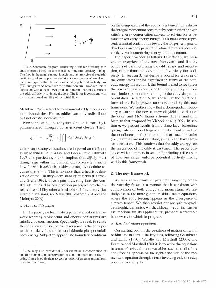
nel of uniform depth, as sketched in Fig. 2. Utilizing an
appropriate d-sheet definition of potential vorticity to
account for surface buoyancy anomalies, it can be shown
that, in a quasigeostrophic framework (Bretherton 1966),
ð ð ðq9y9
zdx dy dz 5 0. (2)
Here, q is the quasigeostrophic potential vorticity; y is
the meridional velocity component; x, y, and z are zonal,
meridional, and vertical Cartesian coordinates; and the
average is evaluated at constant z, consistent with the
quasigeostrophic approximation. This result is clear when
one considers the meridional potential vorticity flux as
the divergence of the Eliassen–Palm flux (Andrews and
FIG. 1. Schematic diagram illustrating a difficulty with eddy
closures based on unconstrained potential vorticity mixing (adap-
ted from Adcock and Marshall 2000). Flow is confined to an abyssal
layer, underlying an infinitely deep, motionless upper layer. (left)
The initial state consists of a set of geostrophically balanced eddies,
associated with a deformed layer interface (solid line), above a
seamount (solid shading). (right) If the eddies were to completely
homogenize the potential vorticity field, this would require the
layer interface to rise completely over the seamount and in turn
a large anticyclonic circulation around the seamount. However, the
energy of this hypothetical end state exceeds that in the initial state,
indicating that unconstrained potential vorticity mixing is physi-
cally impossible.
540 J O U R N A L O F P H Y S I C A L O C E A N O G R A P H Y VOLUME 42
Unauthenticated | Downloaded 03/15/22 01:44 AM UTC
McIntyre 1976), subject to zero normal eddy flux on do-
main boundaries. Hence, eddies can only redistribute
but not create momentum.1
Now suppose that the eddy flux of potential vorticity is
parameterized through a down-gradient closure. Then,
q9y9z
5 2k›qz
›y0
ð ð ðq9y9
zdx dy dz 6¼ 0,
unless very strong constraints are imposed on k (Green
1970; Marshall 1981; White and Green 1982; Killworth
1997). In particular, k . 0 implies that ›qz/›y must
change sign within the domain; or, conversely, a mean
flow for which ›qz/›y is positive or negative definite re-
quires that k 5 0. This is no more than a heuristic deri-
vation of the Charney–Stern stability criterion (Charney
and Stern 1962), once again indicating that the con-
straints imposed by conservation principles are closely
related to stability criteria in classic stability theory (for
related discussions, see Vallis 2006, chapter 6; Wood and
McIntyre 2009).
c. Aims of this paper
In this paper, we formulate a parameterization frame-
work whereby momentum and energy constraints are
satisfied by construction. Specifically, we seek to relate
the eddy stress tensor, whose divergence is the eddy po-
tential vorticity flux, to the total (kinetic plus potential)
eddy energy. Subject to appropriate boundary conditions
on the components of the eddy stress tensor, this satisfies
the integral momentum constraint by construction and can
satisfy energy conservation subject to solving for a pa-
rameterized eddy energy budget. This manuscript repre-
sents an initial contribution toward the longer-term goal of
developing an eddy parameterization that mixes potential
vorticity while conserving energy and momentum.
The paper proceeds as follows. In section 2, we pres-
ent an overview of the new framework and list the
benefits of parameterizing the eddy shape and orienta-
tion, rather than the eddy potential vorticity fluxes di-
rectly. In section 3, we derive a bound for a norm of
the eddy stress tensor expressed in terms of the total
eddy energy. In section 4, this bound is used to reexpress
the stress tensor in terms of the eddy energy and di-
mensionless parameters relating to the eddy shape and
orientation. In section 5, we show that the functional
form of the Eady growth rate is retained by this new
framework. We further show that a down-gradient buoy-
ancy closure in the new framework yields a variant of
the Gent and McWilliams scheme that is similar in
form to that proposed by Visbeck et al. (1997). In sec-
tion 6, we present results from a three-layer baroclinic
quasigeostrophic double-gyre simulation and show that
the nondimensional parameters are of tractable order
(i.e., that they are not vanishingly small) and have large-
scale structure. This confirms that the eddy energy sets
the magnitude of the eddy stress tensor. The paper con-
cludes with a summary in section 7, including a discussion
of how one might enforce potential vorticity mixing
within this framework.
2. The new framework
We seek a framework for parameterizing eddy poten-
tial vorticity fluxes in a manner that is consistent with
conservation of both energy and momentum. We ini-
tially discuss the more general residual-mean equations,
where the eddy forcing appears as the divergence of
a stress tensor. We then restrict our analysis to quasi-
geostrophic dynamics, which, although requiring further
assumptions for its applicability, provides a tractable
framework in which to progress.
a. Residual-mean equations
Our starting point is the equations of motion written in
residual-mean form. The key idea, following Greatbatch
and Lamb (1990), Wardle and Marshall (2000), and
Ferreira and Marshall (2006), is to write the equations
in terms of residual-mean variables, such that all of the
eddy forcing appears on the right-hand side of the mo-
mentum equation through a term involving only the eddy
potential vorticity flux.
FIG. 2. Schematic diagram illustrating a further difficulty with
eddy closures based on unconstrained potential vorticity mixing.
The flow in the zonal channel is such that the meridional potential
vorticity gradient is positive definite. Conservation of zonal mo-
mentum requires that the meridional eddy potential vorticity flux
q9y9z
integrates to zero over the entire domain. However, this is
consistent with a local down-gradient potential vorticity closure if
the eddy diffusivity is identically zero. The latter is consistent with
the unconditional stability of the initial flow.
1 One may also consider this constraint as a conservation of
angular momentum; conservation of zonal momentum in the ro-
tating frame is equivalent to conservation of angular momentum
in an inertial frame.
APRIL 2012 M A R S H A L L E T A L . 541
Unauthenticated | Downloaded 03/15/22 01:44 AM UTC
Recently, Young (2012) has shown that the residual-
mean formulation requires far fewer assumptions than
previously suspected (also see Andrews 1983, for the
zonally averaged case). Assuming only that the buoyancy
increases monotonically with height, Young shows that
the Boussinesq primitive equations can be rewritten in
residual-mean form,
Du
Dt1 f k 3 u 1
$p
r0
5 F 2 $3 � E, (3)
1
r0
›p
›z5 b, (4)
$ � u 1›w
›z5 0, and (5)
Db
Dt5 B. (6)
Here, u and w are the horizontal and vertical velocities,
$ is the horizontal gradient operator, $3 � is the three-
dimensional divergence operator, D/Dt 5 ›/›t 1 u � $ 1
w›/›z is the Lagrangian time derivative, f is the Coriolis
parameter, p is pressure, r0 is the reference density, F
represents explicit mechanical forces, k is the unit ver-
tical vector, b is the buoyancy, and B represents explicit
buoyancy forcing. Eddy forcing is provided by the di-
vergence of a (3 3 2) eddy stress tensor2 E consisting of
the three-dimensional Eliassen–Palm vectors in each
of its columns (see section 2c). The main virtue of this
formulation is that each of the variables in Eqs. (3)–(6)
are defined as residual-mean quantities where the eddy
forcing is confined to the right-hand side of the hori-
zontal momentum equation and nonresidual-mean vari-
ables do not appear. The details of the averaging in
(3)–(6) are complicated, and the reader should refer to
Young (2012) for full details.
For the remainder of this paper, we restrict our atten-
tion to quasigeostrophic dynamics. We make the ap-
proximation that the eddy flux of Rossby–Ertel potential
vorticity along neutral density surfaces is closely related
to the eddy flux of quasigeostrophic potential vorticity
along height surfaces (following Charney and Stern 1962;
Treguier et al. 1997), such that
$3 � E ’ k 3 q9u9z
(7)
(see appendix), where
q 5 =2c 1 by 1›
›z
f 20
N 20
›c
›z
!(8)
is the quasigeostrophic potential vorticity; c is the geo-
strophic streamfunction defined such that u 5 2›c/›y,
y 5 ›c/›x, and f 5 f0 1 by, where f0 and b are constants;
and N0
5N0(z). In (7) and all subsequent expressions,
the average is taken at constant height.
The quasigeostrophic approximation has a number of
obvious disadvantages, including the neglect of finite
variations in bottom topography, the importance of which
has been emphasized in section 1b. Nevertheless, we
hope that the relation between the eddy forcing in the
residual-mean primitive equations and in the quasigeo-
strophic equations presents a clear road map for applying
our ideas to the residual-mean primitive equations in
future manuscripts.
b. Conservation of energy
Having written the equations in residual-mean form,
it is straightforward to evaluate the conversion of en-
ergy between the mean flow and eddies. For quasigeo-
strophic dynamics, the eddy energy equation is
›E
›t1 $3 � ( . . . ) 5 u � k 3 q9u9
z2 DE(E)
5 $c � q9u9z
2 DE(E), (9)
where
E 5$c9 � $c9
z
21
f 20
2N 20
›c9
›z
� �2z
(10)
is the eddy energy and DE
is an operator represent-
ing eddy energy dissipation due to bottom drag (e.g.,
Sen et al. 2008), loss of energy to internal waves (e.g.,
Molemaker et al. 2005; Polzin 2008; Marshall and
Naveira Garabato 2008; Nikurashin and Ferrari 2010),
western boundary dissipation (e.g., Dewar and Hogg
2010; Zhai et al. 2010), and other processes. The term
in brackets on the left-hand side of (9) represents internal
energy fluxes: for example, due to westward Rossby
propagation (Chelton et al. 2007).
Crucially, the first term on the right-hand side of (9)
represents the conversion of energy from the mean flow
to the eddies; a corresponding term appears in the mean
energy equation, such that the total energy (mean plus
2 Young has pointed out that E should be defined as two sep-
arate vectors, because E does not, in general, transform as a ten-
sor (W. R. Young 2011, personal communication). However, in
the quasigeostrophic limit we consider for the remainder of this
paper, E does transform as a tensor under horizontal transforma-
tions and might therefore be termed a ‘‘quasigeostrophic tensor.’’
542 J O U R N A L O F P H Y S I C A L O C E A N O G R A P H Y VOLUME 42
Unauthenticated | Downloaded 03/15/22 01:44 AM UTC
eddy) is conserved aside from explicit energy sources
and sinks. Notwithstanding the challenges of parame-
terizing the internal eddy energy fluxes and eddy energy
dissipation, here we assume that (9) is solved for the
total (kinetic plus potential) eddy energy and we use
this to constrain the magnitude of the eddy stress ten-
sor, as defined in the following subsection. Note that
Eden and Greatbatch (2008), in contrast, solve a prog-
nostic eddy kinetic energy equation and use this to set
the value of the eddy diffusivity, but further approxi-
mations must be applied in constructing an eddy kinetic
energy budget.
c. Eddy stress tensor
Through (7), the residual-mean eddy force, or equiv-
alently the quasigeostrophic eddy potential vorticity
flux, can be expressed as the divergence of an eddy stress
tensor (Plumb 1986). The stress tensor E has columns
equal to the Eliassen–Palm flux vectors and takes the
form
E 5
2M 1 P N
N M 1 P
2S R
0@
1A, (11)
where
M 5y92 2 u92
z
2, N 5 u9y9
z, P 5
b92z
2N 20
,
R 5f0
N 20
b9u9z, and S 5
f0
N 20
b9y9z
(12)
and where f0 is the mean value of the Coriolis param-
eter and N 0 is the buoyancy frequency. Here, M and N
represent the eddy Reynolds stresses associated with
lateral momentum transfer,3 P is the eddy potential en-
ergy. Here, R and S are proportional to the components
of the eddy buoyancy flux; under the quasigeostrophic
approximation, these are in turn equal to the interfacial
eddy form stress associated with vertical momentum
transfer (Munk and Palmen 1951; Johnson and Bryden
1989; Aiki and Richards 2008). Note that P yields a purely
divergent residual-mean force, equivalent to a rotational
potential vorticity eddy flux, and hence the stress due to
P has no influence on the resulting dynamics.
The terms involving M and N, as well as the related
barotropic ‘‘E vector,’’ are discussed in Hoskins et al.
(1983). The lower row (the buoyancy fluxes) contains
exactly those terms that are parameterized in Gent and
McWilliams (1990) and Greatbatch and Lamb (1990).
The surface and bottom boundary conditions for the
eddy form stresses are, neglecting variations in bottom
topography (consistent with the quasigeostrophic ap-
proximation), R 5 S 5 0. On lateral boundaries, M 5
2K cos2f0 and N 5 K sin2f0, where f0 is the angle at
which the boundary is oriented with respect to the x axis
and K is the eddy kinetic energy,
K 5u9 � u9
z
2.
Note that, with no-slip boundaries, which are common in
ocean models, M 5 N 5 0.
Our proposal is to parameterize the four dynamically
relevant components of the eddy stress tensor, M, N, R,
and S, rather than the eddy potential vorticity flux di-
rectly. Note that, although this requires parameteriza-
tion of four eddy fluxes (M, N, R, and S), this is no more
than in the original equations of motion (two eddy Rey-
nolds stresses and two eddy buoyancy fluxes), though
two more than in the residual-mean equations (two
eddy potential vorticity fluxes).
There are number of potential advantages of this
approach:
1) It follows from (7), (11), and the boundary conditions
that appropriate momentum constraints are satisfied.
For example, in a zonal channel (2) is satisfied.
2) It is easily ensured that the parameterized eddy
potential vorticity flux preserves the ‘‘tensorial prop-
erties’’ and symmetries of the original eddy potential
vorticity flux (cf. Popovych and Bihlo 2011, manu-
script submitted to J. Math. Phys.).
3) If we neglect the Reynolds stresses, M and N, then
this formulation reduces to parameterizing the eddy
form stress, as in Gent and McWilliams (1990) and
Greatbatch and Lamb (1990). Thus, the framework is a
natural one to use for extending Gent and McWilliams
to include contributions from Reynolds stresses.
4) The two columns of the eddy stress tensor are the
Eliassen–Palm vectors, associated with the flux of
wave activity, in turn related to the propagation of
eddy energy (Eliassen and Palm 1961; Andrews and
McIntyre 1976). These may provide useful informa-
tion for parameterizing the fluxes of eddy energy.
5) The eddy energy provides a rigorous upper bound on a
norm of the eddy stress tensor (detailed in section 3).
Note that it is the total eddy energy that is bounded,
not the eddy kinetic energy used by Eden and Great-
batch (2008) for which there is no conservation law.
3 Note that the signs of the fluxes M and N are defined in-
consistently in the literature.
APRIL 2012 M A R S H A L L E T A L . 543
Unauthenticated | Downloaded 03/15/22 01:44 AM UTC
6) This upper bound allows the eddy stress tensor to be
rewritten, with no loss of generality, in terms of the
eddy energy, two eddy anisotropy parameters, and
trigonometric factors involving three eddy orienta-
tions. Assuming that the eddy energy is available from
the solution of a parameterized eddy energy equation,
all of the remaining unknowns are nondimensional
and bounded in magnitude by unity. All dimensional
freedom in the parameterization problem is therefore
encapsulated in the eddy energy (section 4).
7) The eddy orientations have a strong connection with
classical stability theory, the eddies extracting energy
from the mean flow when the eddies lean against the
mean shear, and conversely returning energy to the
mean flow when the eddies lean with the mean shear
(section 4).
8) As a result of preserving the symmetries of the
original eddy potential vorticity flux, the framework
is able to retain some results from classical stability
theory, such as the functional form of the Eady
growth rate (section 5) and, with a further constraint
to ensure potential enstrophy is dissipated, Arnold’s
first stability theorem (section 7).
9) Application to the Eady problem suggests a con-
nection between the proposed framework and the
Visbeck et al. (1997) form of the Gent and McWilliams
eddy closure, in the limit of negligible Reynolds
stresses (section 5).
As with any new approach, there are also disadvan-
tages. Here, the most significant disadvantage is the
loss of explicit potential vorticity mixing. On the other
hand, for the reasons outlined in section 1, we argue that
simple-minded down-gradient diffusive closures have
fundamental limitations that, despite four decades of
research (since Green 1970), remain far from being re-
solved, if indeed this is possible (see Ringler and Gent
2011, for a related discussion). In section 7, we propose
a resolution to this particular issue by solving a prognostic
budget for the eddy potential enstrophy, in precisely the
same manner as the eddy energy, and using this budget to
ensure that potential vorticity is mixed on average
through explicit dissipation of eddy potential enstrophy.
3. Bounded norm of the eddy stress tensor
We now proceed to bound the magnitude of the eddy
stress tensor (11) by the eddy energy. This will allow us,
in section 4, to rewrite the eddy stress tensor in terms
of the eddy energy and bounded nondimensional pa-
rameters.
First, we note that the components of the eddy stress
tensor, M and N, are bounded by
M2 1 N2 # K2, (13)
where K is the eddy kinetic energy (Hoskins et al. 1983).
To prove (13), note that the result is an equality at any
instant in time, before averaging, then apply the triangle
inequality to the integral in the averaging operator. Sec-
ond, we note that P is exactly the eddy potential energy.
Third, again through application of the triangle in-
equality, we have
N 20
2f 20
(R2 1 S2) # 2KP #E2
2. (14)
The latter inequality follows by noting P 5 E 2 K and
maximizing the resultant quadratic.
Summing each of the above results, we obtain the final
result,
1
2(2M 1 P)2
1 N2 1 N2 1 (M 1 P)21N 2
0
f 20
(R2 1 S2)
" #
5 M2 1 N2 1 P2 1N 2
0
2f 20
(R2 1 S2) # E2, (15)
where E is the total eddy energy as defined in Eq. (10).
The left-hand side of (15) represents a weighted4 Fro-
benius norm of the eddy stress tensor and bounds its
magnitude. Note that the bound is expressed in terms of
the total eddy energy and not simply the eddy kinetic
energy used to set the magnitude of the eddy diffusivity
in Eden and Greatbatch (2008). Physically, a finite eddy
buoyancy flux requires both eddy kinetic energy, for fi-
nite u9, and eddy potential energy, for finite b9.
4. Eddy flux angles and eddy anisotropies
Without any loss of generality, the bound (15) allows
us to rewrite the components of the eddy stress tensor
for an arbitrary eddy field in the form
M 5 2gmE cos2fm cos2l, N 5 gmE sin2fm cos2l,
P 5 E sin2l, R 5 gb
f0
N 0
E cosfb sin2l,
S 5 gb
f0
N 0
E sinfb sin2l. (16)
Here, we have introduced two eddy anisotropies, 0 # gm #
1 and 0 # gb # 1; two eddy flux angles, 0 # fm # p and
4 Weighting of vertical components by factors of N0/f
0occurs
frequently in quasigeostrophic theory.
544 J O U R N A L O F P H Y S I C A L O C E A N O G R A P H Y VOLUME 42
Unauthenticated | Downloaded 03/15/22 01:44 AM UTC
2p # fb # p; and an eddy energy partition angle, 0 # l
# p/2. Thus, eddy fluxes are recast in terms of six pa-
rameters, five of which are independent. Five of the pa-
rameters are dimensionless and bounded, with the only
remaining dimensional parameter being the eddy energy
E. In the limit of plane waves, it follows that gm 5 gb 5 1
and fm 5 fb 5 f9, the angle of phase propagation.
The anisotropy parameter gm measures the relative
magnitudes of the Reynolds stresses and eddy kinetic
energy,
gm 5
ffiffiffiffiffiffiffiffiffiffiffiffiffiffiffiffiffiffiffiffiM2 1 N2
pK
. (17)
Similarly, the anisotropy parameter gb measures the rel-
ative magnitude of the eddy buoyancy fluxes to the
(square root of the) kinetic and potential energies,
gb 5N 0
2f0
ffiffiffiffiffiffiffiffiffiffiffiffiffiffiffiffiffiR2 1 S2
KP
s. (18)
One can further define a ‘‘net anisotropy’’ parameter,
ge 51
E
ffiffiffiffiffiffiffiffiffiffiffiffiffiffiffiffiffiffiffiffiffiffiffiffiffiffiffiffiffiffiffiffiffiffiffiffiffiffiffiffiffiffiffiffiffiffiffiffiffiffiffiffiffiffiffiffiffiffiffiffiffiffiffiffiffiffiffiM2 1 N2 1 P2 1
N 20
2f 20
(R2 1 S2)
s, (19)
where 0 # ge # 1. This quantifies the extent to which the
bound (15) constrains the magnitude of the eddy fluxes.
It follows that ge, gm, and gb are related through
(1 2 g2e) 5 (1 2 g2
m) cos4l 11
2(1 2 g2
b) sin22l. (20)
However, ge contains no additional information to that
already contained within gm, gb, and l.
The angles fm and fb measure the dominant orien-
tation of the eddy momentum and buoyancy fluxes,
cos2fm 5 2Mffiffiffiffiffiffiffiffiffiffiffiffiffiffiffiffiffiffiffiffi
M2 1 N2p , cosfb 5
RffiffiffiffiffiffiffiffiffiffiffiffiffiffiffiffiffiR2 1 S2
p . (21)
Note that there is a p rotation symmetry in M and N
as opposed to a 2p rotation symmetry in R and S, con-
sistent with the symmetry of the original eddy fluxes.
Thus, parameterizing these angles ensures that the com-
ponents of the eddy stress tensor retain the correct rota-
tional symmetries. The angle l measures the partitioning
of eddy energy between kinetic and potential forms,
K
E5 cos2l,
P
E5 sin2l. (22)
For an elliptical horizontal eddy, shown in Fig. 3a, it
follows that fm is the angle of eddy orientation and gm
is a measure of the eddy eccentricity in the horizontal,
gm 5c2
1 2 c22
c21 1 c2
2
, (23)
where c1 and c2 are as shown in Fig. 3a. This interpre-
tation of fm and gm has previously been derived in
Hoskins et al. (1983).
The terms gb and l measure the vertical shape of
the eddies. The buoyancy fluxes can be written equiva-
lently as
R 5 gt
f0
N 0
E sin2ft cosfb, S 5 gt
f0
N 0
E sin2ft sinfb,
where gt and ft are defined such that
tan2ft 5 gb tan 2l, gt 5cos2l
cos2ft
and where it is easily shown that 0 # gb # gt # 1. Then,
for a vertically planar elliptical eddy, shown in Fig. 3b,
it follows that ft is the angle of eddy tilt in the vertical
and gt is a measure of the eccentricity,
gt 5d2
1 2 d22
d21 1 d2
2
, (24)
where d1 and d2 are as shown in Fig. 3b.
This geometric interpretation of the eddy fluxes
also provides a strong physical connection with linear
stability theory (Pedlosky 1987, chapter 7), illustrated
schematically in Fig. 4. Eddies extract energy from the
mean flow when they lean into the shear, consistent with
instability; conversely, eddies return energy to the mean
flow when they lean with the shear, consistent with sta-
bility. A related discussion of observed and modeled
eddy Reynolds stresses decelerating and accelerating
the Kuroshio is given in Waterman et al. (2011, partic-
ularly their Fig. 24); also see Greatbatch et al. (2010) for
an illustration of eddy Reynolds stresses accelerating the
separated Gulf Stream.
5. Application to the Eady model
In the next two sections, we apply the new framework
to two limiting cases: (i) baroclinic instability in a chan-
nel and (ii) fully developed turbulence in a closed, wind-
driven basin.
Following Eady (1949), we consider a uniform bar-
oclinic shear in an infinite zonal channel,
APRIL 2012 M A R S H A L L E T A L . 545
Unauthenticated | Downloaded 03/15/22 01:44 AM UTC
u 5 Lz 0 c 5 2Lyz 0 b 5 2f0Ly.
The Coriolis parameter is assumed constant (i.e., f 5 f0),
and hence the potential vorticity is uniform at each level,
Q 5 f0, except at the upper and lower boundaries, where
we interpret the buoyancy gradients as a d sheet of po-
tential vorticity anomalies following the approach of
Bretherton (1966). Eady theory predicts that the energy
of the most unstable mode on this background shear
grows at a rate,
2T 21Eady ’ 0:62
f0L
N 0
. (25)
Note that this is twice the growth rate of the eddy
streamfunction and other linear eddy quantities.
a. Eady growth rate in the new parameterizationframework
We first show that the functional form of the Eady
growth rate is automatically retained by the new param-
eterization framework. The global eddy energy budget is
›
›t
ð ð ðE dx dy dz 5 2
ð ð ðuq9y9
zdxdy dz
5
ð ð ðLS dx dy dz. (26)
The terms involving M and N integrate out through the
boundary conditions. Assuming only that S is directed
down the mean buoyancy gradient, necessary for the
eddy energy to grow, and
S 5 af0E
N 0
from (16), where a 5 gb sinfb sin2l # 1 is an un-
determined nondimensional parameter, we find
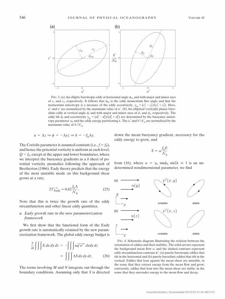
FIG. 3. (a) An elliptic barotropic eddy at horizontal angle fm and with major and minor axes
of c1 and c2, respectively. It follows that fm is the eddy momentum flux angle and that the
momentum anisotropy is a measure of the eddy eccentricity, gm 5 (c21 2 c2
2)/(c21 1 c2
2). Here,
u9 and y9 are normalized by the maximum value of u9. (b) An elliptical vertically planar baro-
clinic eddy at vertical angle ft and with major and minor axes of d1 and d2, respectively. The
eddy tilt ft and eccentricity gm 5 (d21 2 d2
2)/(d21 1 d2
2) are determined by the buoyancy anisot-
ropy parameter gb and the eddy energy partitioning l. The u9 and b9/N 0 are normalized by the
maximum value of b9/N0.
FIG. 4. Schematic diagram illustrating the relation between the
orientation of eddies and their stability. The solid arrows represent
the background mean flow u, and the dashed contours represent
eddy streamfunction contours c9: (a) purely barotropic eddies that
tilt in the horizontal and (b) purely baroclinic eddies that tilt in the
vertical. Eddies that lean against the mean shear are unstable, in
the sense that they extract energy from the mean flow and grow;
conversely, eddies that lean into the mean shear are stable, in the
sense that they surrender energy to the mean flow and decay.
546 J O U R N A L O F P H Y S I C A L O C E A N O G R A P H Y VOLUME 42
Unauthenticated | Downloaded 03/15/22 01:44 AM UTC
›
›t
ð ð ðE dx dy dz 5
ð ð ða
f0L
N 0
E dx dy dz
5 ~af0L
N 0
ð ð ðE dx dy dz, (27)
where ~a # amax # 1.
Thus, without specifying the form of the eddy closure
for the components of the stress tensor, other than that
the eddy buoyancy flux is on average down the mean
buoyancy gradient, this new approach is guaranteed to
preserve the functional form of the Eady growth rate,
with an upper bound that is within a factor of 0.62 of
the growth rate actually obtained. This is in marked
contrast to previous down-gradient eddy closures in
which arbitrary, dimensional eddy diffusivities need to be
specified.5
b. A down-gradient buoyancy closure in the newparameterization framework
As shown above, the eddy Reynolds stresses have no
integral effect on the eddy energy growth in the Eady
problem, effectively reducing to the new approach to
that employed by Gent and McWilliams (1990) and sub-
sequent extensions. We now consider a general down-
gradient buoyancy closure and infer an effective eddy
diffusivity. Writing
b9u9z
5N 2
0
f0
(R, S) 5 N 0Egb sin2l(cosfb, sinfb) (28)
and applying a down-gradient buoyancy closure,
b9u9z
5 2k$bz, (29)
it follows that
k 5 aE
ffiffiffiffiffiffiRip
f0
, (30)
where a 5 gb sin2l is a nondimensional constant, boun-
ded by unity in magnitude, and Ri 5N 20/j›u/›zj2 is the
Richardson number. This is a general form of the Gent and
McWilliams coefficient in a quasigeostrophic framework.
We can, for example, relate this form for the Gent and
McWilliams coefficient to Visbeck et al. (1997). Assum-
ing equipartition of eddy energy yields E ’ 2K ’ u2eddy,
where ueddy is an eddy velocity. Following Green (1970)
and Stone (1972), the eddy velocity can be approximated
as an eddy length scale divided by the Eady growth rate,
ueddy ’ l/T Eady, yielding the result
k ’ af0ffiffiffiffiffiffiRip l2. (31)
This is precisely the form proposed by Visbeck et al.
(1997), which drops out of the new formulation as a nat-
ural limiting case. Note, however, that because of ambi-
guity in the definition of the eddy length scale, the
coefficient a that appears here can no longer be bounded.
Of the parameters in (30), Ri depends upon the mean
flow, whereas a and E are properties of the eddies.
Hence a down-gradient buoyancy closure in this general
form requires a parameterized eddy energy budget and
a parameterization for a. Note, however, that Visbeck
et al. (1997) find in numerical experiments that the
constant a in (31) has little spatial dependence. It should
also be noted that, in stable regions of the flow, corre-
sponding to regions of high Richardson number and to
large Eady growth time scales, the coefficient prescribed
by (30) becomes the product of a small eddy energy
(as the flow is stable) but a large Eady growth time
scale. This potentially complicates the direct application
of this functional form of the Gent and McWilliams
coefficient.
6. Application to wind-driven gyres
The eddy stress tensor decomposition (11) is general,
but it is not self-evidently applicable as a framework for
eddy parameterization. In particular, should the an-
isotropy parameters be small or should any of the pa-
rameters exhibit finescale spatial structure, then the
potential vorticity fluxes would be highly sensitive to
the details of their parameterization. In such a situa-
tion, the problem of parameterizing the geometric pa-
rameters would be highly intractable and could not be
expected to capture the influence of the eddies on the
mean flow.
In this section, we investigate, in an idealized ocean-
ographic context exhibiting fully developed geostrophic
turbulence, whether the nondimensional parameters have
a magnitude of tractable order for the purposes of pa-
rameterization (i.e., that they have an order close to
unity). We further investigate whether the parameters of
the flux decomposition exhibit large-scale structure with
features relating to the mean flow structure. For these
purposes, we use a three-layer quasigeostrophic model
to simulate a baroclinic double-gyre configuration, as de-
scribed in Berloff et al. (2007).
5 Conversely, if we assume S is directed up the mean buoyancy
gradient, then the same result is obtained, except with the opposite
sign on the right-hand side of (27); this corresponds to eddy decay
(i.e., to the stable Eady mode).
APRIL 2012 M A R S H A L L E T A L . 547
Unauthenticated | Downloaded 03/15/22 01:44 AM UTC
a. Model configuration
The three-layer quasigeostrophic equations are dis-
cretized using a potential vorticity–conserving, second-
order centered finite difference formulation in space and
using the leapfrog method in time with a Robert–
Asselin filter of strength 0.1 in time. The simulations are
conducted in a square domain 2L # x # L, 2L # y # L
with a partial-slip boundary condition applied at all
lateral boundaries. The model parameters are listed in
Table 1 and correspond to a Reynolds number, defined
using the upper-ocean Sverdrup velocity scale U 5 t0/
(r1H1Lb) of Re 5 1600 and a Munk boundary layer scale
of dM 5 (n/b)1/3 5 17 km. An asymmetric wind forcing
is applied, equivalent to a prescribed Ekman upwelling
velocity in the upper layer,
wEk 5 2pt0
r0f0L
1
Asin
p(L 1 y)
L 1 Bxfor y # Bx,
1pt0
r0 f0LA sin
�p(y 2 Bx)
L 2 Bx
�for y . Bx,
where A 5 1.1 generates an asymmetric wind stress
amplitude in each gyre, B 5 0.2 creates a moderate tilt
of the zero wind stress line to the x axis, and t0 is a pre-
scribed parameter that sets the magnitude of the wind
stress.
The model is integrated using a uniform grid with 513
nodes in the meridional and zonal directions, corre-
sponding to 7.5-km resolution and with a time step size
of 1800 s. The model is integrated for 20 000 days, until
a statistical equilibrium is reached (determined using
measurements of the flow kinetic and potential energy),
and then integrated for a further 50 000 days, with the
eddy fluxes (12) computed based upon a time average
over this full 50 000-day window. These eddy fluxes are
decomposed into the eddy energy, the eddy anisotropies,
and the eddy angles following (16). Because the buoyancy
is defined at model layer interfaces and the velocity is
defined within layers, the buoyancy fluxes R and S are
computed within each layer by averaging the buoyancy
between the two adjacent interfaces. The eddy energy is
diagnosed by rewriting in the form
E 5=2c92
z
41
›
›z
f 20
4N 20
›c92z
›z
!2
q9c9z
2,
where this latter expression is naturally computed within
each layer. The eddy potential energy is diagnosed as
the residual of the eddy energy and eddy kinetic energy,
P 5 E 2 K.
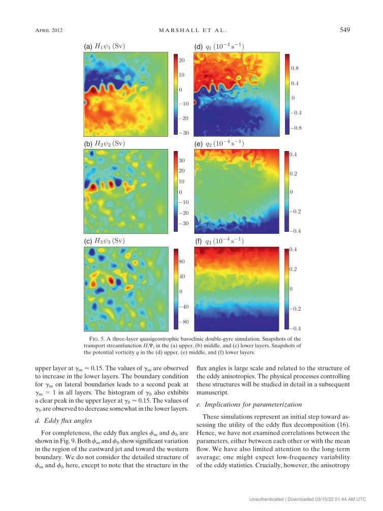
Figure 5 shows the final instantaneous transport stream-
function and potential vorticity. One sees the expected
characteristic double-gyre regime, with an intense east-
ward jet separating two gyres and with transient eddies
observed throughout the domain. Partial homogenization
of mean potential vorticity in the middle layer and in the
central part of the domain is also observed (Holland and
Rhines 1980; Rhines and Young 1982a,b).
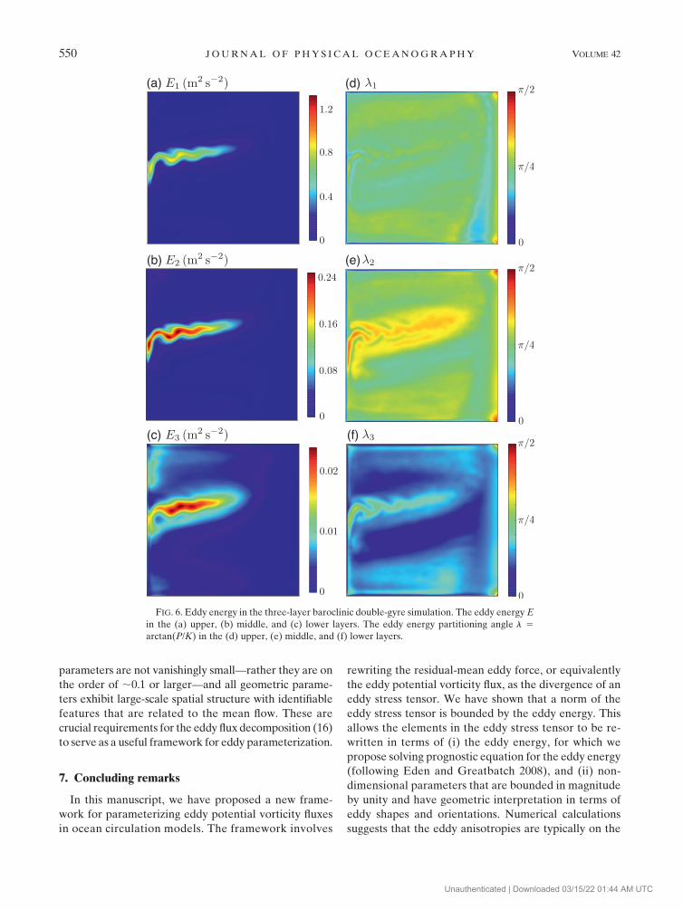
b. Eddy energy
The eddy energy and eddy energy partitioning angle l
are shown in Fig. 6. The eddy energy is primarily con-
centrated in the thin eastward jet, and it decreases in the
lower layers, as expected. The eddy energy partitioning
indicates that the energy is approximately equipartitioned
between potential and kinetic parts, with a slightly larger
potential energy part in the middle larger and kinetic part
in the lower layer. The normalized histogram of the par-
titioning angle l peaks at values of 0.25p, 0.28p, and
0.16p in the upper, middle, and lower layers, respectively.
Elevated values of l, indicating relatively increased po-
tential energy, are observed in the eastward jet and in the
western boundary region.
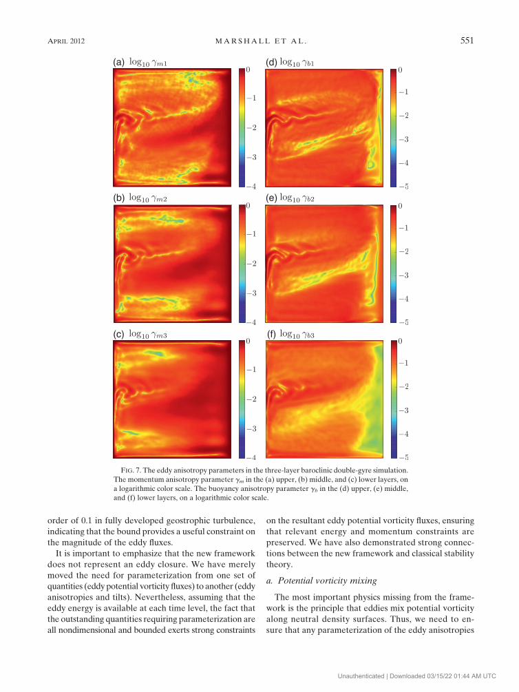
c. Eddy anisotropies
The momentum anisotropy gm and the buoyancy an-
isotropy gb are shown in Fig. 7. Significant structure is
observed in the momentum anisotropy parameter gm,
with larger values of gm observed toward the eastern
boundary. A thin zonal line of low momentum anisotropy
is observed near the northern and southern boundaries.
The buoyancy anisotropy gb also exhibits some signif-
icant structure. In particular, two clear tracks of in-
creased buoyancy anisotropy are observed on the flanks
of the eastward jet in the upper and middle layers.
Somewhat decreased values of the buoyancy anisotropy
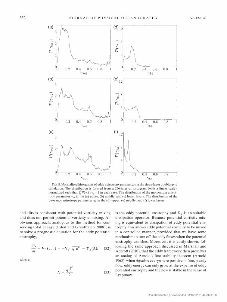
are observed in the recirculation regions. The normal-
ized histograms of gm and gb in each layer are shown in
Fig. 8. The histogram of gm exhibits a clear peak in the
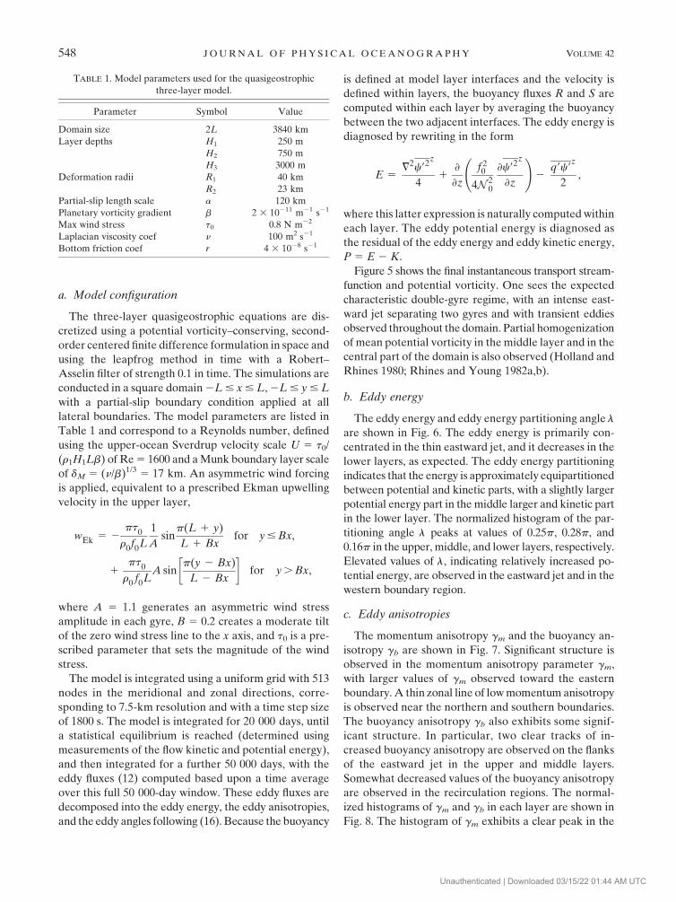
TABLE 1. Model parameters used for the quasigeostrophic
three-layer model.
Parameter Symbol Value
Domain size 2L 3840 km
Layer depths H1 250 m
H2 750 m
H3 3000 m
Deformation radii R1 40 km
R2 23 km
Partial-slip length scale a 120 km
Planetary vorticity gradient b 2 3 10211 m21 s21
Max wind stress t0 0.8 N m22
Laplacian viscosity coef n 100 m2 s21
Bottom friction coef r 4 3 1028 s21
548 J O U R N A L O F P H Y S I C A L O C E A N O G R A P H Y VOLUME 42
Unauthenticated | Downloaded 03/15/22 01:44 AM UTC
upper layer at gm ’ 0.15. The values of gm are observed
to increase in the lower layers. The boundary condition
for gm on lateral boundaries leads to a second peak at
gm 5 1 in all layers. The histogram of gb also exhibits
a clear peak in the upper layer at gb ’ 0.15. The values of
gb are observed to decrease somewhat in the lower layers.
d. Eddy flux angles
For completeness, the eddy flux angles fm and fb are
shown in Fig. 9. Both fm and fb show significant variation
in the region of the eastward jet and toward the western
boundary. We do not consider the detailed structure of
fm and fb here, except to note that the structure in the
flux angles is large scale and related to the structure of
the eddy anisotropies. The physical processes controlling
these structures will be studied in detail in a subsequent
manuscript.
e. Implications for parameterization
These simulations represent an initial step toward as-
sessing the utility of the eddy flux decomposition (16).
Hence, we have not examined correlations between the
parameters, either between each other or with the mean
flow. We have also limited attention to the long-term
average; one might expect low-frequency variability
of the eddy statistics. Crucially, however, the anisotropy
FIG. 5. A three-layer quasigeostrophic baroclinic double-gyre simulation. Snapshots of the
transport streamfunction HiCi in the (a) upper, (b) middle, and (c) lower layers. Snapshots of
the potential vorticity q in the (d) upper, (e) middle, and (f) lower layers.
APRIL 2012 M A R S H A L L E T A L . 549
Unauthenticated | Downloaded 03/15/22 01:44 AM UTC
parameters are not vanishingly small—rather they are on
the order of ;0.1 or larger—and all geometric parame-
ters exhibit large-scale spatial structure with identifiable
features that are related to the mean flow. These are
crucial requirements for the eddy flux decomposition (16)
to serve as a useful framework for eddy parameterization.
7. Concluding remarks
In this manuscript, we have proposed a new frame-
work for parameterizing eddy potential vorticity fluxes
in ocean circulation models. The framework involves
rewriting the residual-mean eddy force, or equivalently
the eddy potential vorticity flux, as the divergence of an
eddy stress tensor. We have shown that a norm of the
eddy stress tensor is bounded by the eddy energy. This
allows the elements in the eddy stress tensor to be re-
written in terms of (i) the eddy energy, for which we
propose solving prognostic equation for the eddy energy
(following Eden and Greatbatch 2008), and (ii) non-
dimensional parameters that are bounded in magnitude
by unity and have geometric interpretation in terms of
eddy shapes and orientations. Numerical calculations
suggests that the eddy anisotropies are typically on the
FIG. 6. Eddy energy in the three-layer baroclinic double-gyre simulation. The eddy energy E
in the (a) upper, (b) middle, and (c) lower layers. The eddy energy partitioning angle l 5
arctan(P/K) in the (d) upper, (e) middle, and (f) lower layers.
550 J O U R N A L O F P H Y S I C A L O C E A N O G R A P H Y VOLUME 42
Unauthenticated | Downloaded 03/15/22 01:44 AM UTC
order of 0.1 in fully developed geostrophic turbulence,
indicating that the bound provides a useful constraint on
the magnitude of the eddy fluxes.
It is important to emphasize that the new framework
does not represent an eddy closure. We have merely
moved the need for parameterization from one set of
quantities (eddy potential vorticity fluxes) to another (eddy
anisotropies and tilts). Nevertheless, assuming that the
eddy energy is available at each time level, the fact that
the outstanding quantities requiring parameterization are
all nondimensional and bounded exerts strong constraints
on the resultant eddy potential vorticity fluxes, ensuring
that relevant energy and momentum constraints are
preserved. We have also demonstrated strong connec-
tions between the new framework and classical stability
theory.
a. Potential vorticity mixing
The most important physics missing from the frame-
work is the principle that eddies mix potential vorticity
along neutral density surfaces. Thus, we need to en-
sure that any parameterization of the eddy anisotropies
FIG. 7. The eddy anisotropy parameters in the three-layer baroclinic double-gyre simulation.
The momentum anisotropy parameter gm in the (a) upper, (b) middle, and (c) lower layers, on
a logarithmic color scale. The buoyancy anisotropy parameter gb in the (d) upper, (e) middle,
and (f) lower layers, on a logarithmic color scale.
APRIL 2012 M A R S H A L L E T A L . 551
Unauthenticated | Downloaded 03/15/22 01:44 AM UTC
and tilts is consistent with potential vorticity mixing
and does not permit potential vorticity unmixing. An
obvious approach, analogous to the method for con-
serving total energy (Eden and Greatbatch 2008), is
to solve a prognostic equation for the eddy potential
enstrophy,
›L
›t1 $ � ( . . . ) 5 2$q � q9u9
z2 D
L(L), (32)
where
L 5q92
z
2(33)
is the eddy potential enstrophy and DL
is an suitable
dissipation operator. Because potential vorticity mix-
ing is equivalent to dissipation of eddy potential ens-
trophy, this allows eddy potential vorticity to be mixed
in a controlled manner, provided that we have some
mechanism to turn off the eddy fluxes when the potential
enstrophy vanishes. Moreover, it is easily shown, fol-
lowing the same approach discussed in Marshall and
Adcroft (2010), that the eddy framework then preserves
an analog of Arnold’s first stability theorem (Arnold
1965): when dq/dc is everywhere positive in free, steady
flow, eddy energy can only grow at the expense of eddy
potential enstrophy and the flow is stable in the sense of
Lyapunov.
FIG. 8. Normalized histograms of eddy anisotropy parameters in the three-layer double-gyre
simulation. The distribution is formed from a 256-interval histogram (with a linear scale),
normalized such thatÐ 1
0P(gi) dgi 5 1 in each case. The distribution of the momentum anisot-
ropy parameter gm in the (a) upper, (b) middle, and (c) lower layers. The distribution of the
buoyancy anisotropy parameter gb in the (d) upper, (e) middle, and (f) lower layers.
552 J O U R N A L O F P H Y S I C A L O C E A N O G R A P H Y VOLUME 42
Unauthenticated | Downloaded 03/15/22 01:44 AM UTC
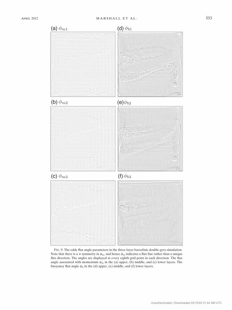
FIG. 9. The eddy flux angle parameters in the three-layer baroclinic double-gyre simulation.
Note that there is a p symmetry in fm, and hence fm indicates a flux line rather than a unique
flux direction. The angles are displayed at every eighth grid point in each direction. The flux
angle associated with momentum fm in the (a) upper, (b) middle, and (c) lower layers. The
buoyancy flux angle fb in the (d) upper, (e) middle, and (f) lower layers.
APRIL 2012 M A R S H A L L E T A L . 553
Unauthenticated | Downloaded 03/15/22 01:44 AM UTC
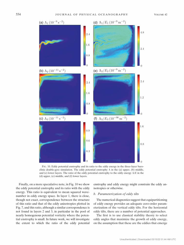
Finally, on a more speculative note, in Fig. 10 we show
the eddy potential enstrophy and its ratio with the eddy
energy. This ratio is equivalent to mean squared wave-
number in eddy energy space. In layer 1, there is close,
though not exact, correspondence between the structure
of this ratio and that of the eddy anisotropies plotted in
Fig. 7, and this ratio, although a similar correspondence is
not found in layers 2 and 3, in particular in the pool of
nearly homogenous potential vorticity where the poten-
tial enstrophy is small. In future work, we will investigate
the extent to which the ratio of the eddy potential
enstrophy and eddy energy might constrain the eddy an-
isotropies or otherwise.
b. Parameterization of eddy tilts
The numerical diagnostics suggest that equipartitioning
of eddy energy provides an adequate zero-order param-
eterization of the vertical eddy tilts. For the horizontal
eddy tilts, there are a number of potential approaches.
The first is to use classical stability theory to select
eddy angles that maximize the growth of eddy energy,
on the assumption that these are the eddies that emerge
FIG. 10. Eddy potential enstrophy and its ratio to the eddy energy in the three-layer baro-
clinic double-gyre simulation. The eddy potential enstrophy L in the (a) upper, (b) middle,
and (c) lower layers. The ratio of the eddy potential enstrophy to the eddy energy L/E in the
(d) upper, (e) middle, and (f) lower layers.
554 J O U R N A L O F P H Y S I C A L O C E A N O G R A P H Y VOLUME 42
Unauthenticated | Downloaded 03/15/22 01:44 AM UTC
at finite amplitude. The second is to select eddy angles
that maximize mixing of potential vorticity, although
preliminary results suggest that such an approach requires
calculation of high-order derivatives and is impractical.
Alternatively, to the extent that the eddies can be
modeled as linear waves, one might use ray-tracing the-
ory (e.g., Buhler 2009) to determine how the eddies are
deformed by the background shear. Intriguingly, the ray-
tracing formulation is also closely related to the propa-
gation of wave activity, in turn related to the propagation
(and growth) of eddy energy. It is therefore possible that
a ray-tracing approach could be used simultaneously to
solve for the propagation and growth of eddy energy as
well as the deformation of eddies by the mean flow.
c. Divergent eddy potential vorticity fluxes
The new framework relates the total eddy potential
vorticity flux to the divergence of the eddy stress tensor.
However, it is only the divergent component of the eddy
potential vorticity flux that influences the evolution of the
mean flow; the rotational flux results in a divergent force
on the right-hand side of the momentum Eq. (3) that
projects on the pressure gradient and has no influence on
the evolution of the flow (in the three-dimensional, non-
quasigeostrophic residual-mean equations, the divergent
and rotational fluxes must be defined through a three-
dimensional decomposition; cf. Marshall and Pillar 2011).
An important issue is therefore the extent to which
the new framework provides useful constraints on the
magnitude and structure of the divergent, rather than
full, eddy potential vorticity fluxes. Previous diagnostics
of rotational and divergent eddy potential vorticity
fluxes suggest that the latter are typically an order of
magnitude smaller (Marshall and Shutts 1981; Roberts
and Marshall 2000). The new framework includes an
explicit rotational potential vorticity flux through the
contribution of the eddy potential energy, but it is likely
that the remaining terms also project significantly onto
the rotational eddy potential vorticity flux.
d. Application to the primitive equations
Finally, although we have focused on quasigeostrophic
eddy potential vorticity fluxes in this manuscript, for
reasons of analytical tractability, the fact that eddy fluxes
of Rossby–Ertel potential vorticity appear on the right-
hand side of the residual-mean Eq. (3) provides a clear
road map for applying any parameterization developed
using the new framework directly to the primitive equa-
tions. Although this will require further assumptions, the
use of an eddy stress tensor means that it should be
straightforward to enforce any momentum constraints.
We also anticipate that the application of the new frame-
work to the primitive equations may be of value for
studying the influence of variable bottom topography
on the eddy potential vorticity fluxes and their forcing
of mean flows.
Acknowledgments. We wish to thank Geoff Vallis and
an anonymous reviewer for exceptionally constructive and
thorough reviews that led to a much improved manu-
script. We also thank Bill Young and Xiaoming Zhai for
additional insightful comments. Financial support was
provided by the UK Natural Environment Research
Council (NE/H020454/1).
APPENDIX
Quasigeostrophic Residual-Mean Equations
The time-filtered quasigeostrophic momentum and
buoyancy equations can be written as
Dgug
Dt1 byk 3 ug 1 f0k 3 uag 1 $
pag
r0
1u9 � u9
z
2
!
5 F 2 k 3 z9u9z
and (A1)
Dgb
Dt1 wN 2
0 5 B 2 $ � b9u9z, (A2)
where z is the relative vorticity and subscripts (. . .)g and
(. . .)ag indicate geostrophic and ageostrophic components.
Now, define the nondivergent eddy bolus velocity
(Gent et al. 1995),
u* 5 2›
›z
b9u9z
N 20
!, w* 5 $ � b9u9
z
N 20
!. (A3)
This allows the momentum and buoyancy equations to
be rewritten in residual-mean form,
Dgug
Dt1 byk 3 ug 1 f0k 3 (uag 1 u*)
1 $pag
r0
1 K 2 P
� �5 F 2 k 3 q9u9
zand (A4)
Dgb
Dt1 (w 1 w*)N 2
0 5 B, (A5)
where K and P are the eddy kinetic and potential
energies. Explicit eddy forcing appears only in the
momentum equation, through the eddy potential vor-
ticity flux. The ageostrophic velocity, (uag, w), is re-
placed by a residual ageostrophic velocity, (uag 1 u*, w 1
w*), and the ageostrophic pressure is replaced by
a modified pressure, pag 1 r0(K 2 P), neither of which
affects the evolution of the geostrophic flow.
APRIL 2012 M A R S H A L L E T A L . 555
Unauthenticated | Downloaded 03/15/22 01:44 AM UTC
REFERENCES
Adcock, S. T., and D. P. Marshall, 2000: Interactions between
geostrophic eddies and the mean circulation over large-scale
bottom topography. J. Phys. Oceanogr., 30, 3223–3238.
Aiki, H., and K. J. Richards, 2008: Energetics of the global ocean:
The role of layer-thickness form drag. J. Phys. Oceanogr., 38,
1845–1869.
Andrews, D. G., 1983: A finite-amplitude Eliassen-Palm theorem
in isentropic coordinates. J. Atmos. Sci., 40, 1877–1883.
——, and M. E. McIntyre, 1976: Planetary waves in a horizontal
and vertical shear: The generalized Eliassen-Palm relation and
the mean zonal acceleration. J. Atmos. Sci., 33, 2031–2048.
Arnold, V. I., 1965: Conditions for nonlinear stability of stationary
plane curvilinear flows of an ideal fluid. Dokl. Akad. Nauk
SSSR, 162, 975–978.
Berloff, P., A. M. C. Hogg, and W. Dewar, 2007: The turbulent
oscillator: A mechanism of low-frequency variability of the
wind-driven ocean gyres. J. Phys. Oceanogr., 37, 2363–2386.
Bretherton, F. P., 1966: Critical layer instability in baroclinic flows.
Quart. J. Roy. Meteor. Soc., 92, 325–334.
——, and D. B. Haidvogel, 1976: Two-dimensional turbulence
above topography. J. Fluid Mech., 78, 129–154.
Buhler, O., 2009: Waves and Mean Flows. Cambridge University
Press, 341 pp.
Charney, J. G., and M. E. Stern, 1962: On the stability of internal
baroclinic jets in a rotating atmosphere. J. Atmos. Sci., 19, 159–
172.
Chelton, D. B., M. G. Schlax, R. M. Samelson, and R. A. de Szoeke,
2007: Global observations of large oceanic eddies. Geophys.
Res. Lett., 34, L15606, doi:10.1029/2007GL030812.
Cummins, P. F., 1992: Inertial gyres in decaying and forced geo-
strophic turbulence. J. Mar. Res., 50, 545–566.
Danabasoglu, G., J. C. McWilliams, and P. R. Gent, 1994: The role
of mesoscale tracer transports in the global ocean circulation.
Science, 264, 1123–1126.
Dewar, W. K., and A. M. Hogg, 2010: Topographic inviscid dissi-
pation of balanced flow. Ocean Modell., 32, 1–13.
Eady, E. T., 1949: Long waves and cyclone waves. Tellus, 1, 33–52.
Eden, C., 2010: Parameterising meso-scale eddy momentum fluxes
based on potential vorticity mixing and a gauge term. Ocean
Modell., 32, 58–71.
——, and R. J. Greatbatch, 2008: Towards a mesoscale eddy clo-
sure. Ocean Modell., 20, 223–239.
Eliassen, A., and E. Palm, 1961: On the transfer of energy in sta-
tionary mountain waves. Geofys. Publ., 22, 1–23.
Ferreira, D., and J. Marshall, 2006: Formulation and implementation
of a ‘‘residual-mean’’ ocean circulation model. Ocean Modell.,
13, 86–107.
Gent, P. R., 2011: The Gent-McWilliams parameterization: 20/20
hindsight. Ocean Modell., 39, 2–9.
——, and J. C. McWilliams, 1990: Isopycnal mixing in ocean cir-
culation models. J. Phys. Oceanogr., 20, 150–155.
——, J. Willebrand, T. J. McDougall, and J. C. McWilliams, 1995:
Parameterizing eddy-induced tracer transports in ocean cir-
culation models. J. Phys. Oceanogr., 25, 463–474.
Greatbatch, R. J., and K. G. Lamb, 1990: On parameterizing ver-
tical mixing of momentum in non-eddy resolving ocean models.
J. Phys. Oceanogr., 20, 1634–1637.
——, X. Zhai, M. Claus, L. Czeschel, and W. Rath, 2010: Transport
driven by eddy momentum fluxes in the Gulf Stream Ex-
tension region. Geophys. Res. Lett., 37, L24401, doi:10.1029/
2010GL045473.
Green, J. S. A., 1970: Transfer properties of the large-scale eddies
and the general circulation of the atmosphere. Quart. J. Roy.
Meteor. Soc., 96, 157–185.
Hecht, M. W., and R. D. Smith, 2008: Towards a physical un-
derstanding of the North Atlantic: A review of model studies
in an eddying regime. Ocean Modeling in an Eddying Re-
gime, Geophys. Monogr., Vol. 177, Amer. Geophys. Union,
213–240.
Holland, W. R., and P. B. Rhines, 1980: An example of eddy-induced
circulation. J. Phys. Oceanogr., 10, 1010–1031.
Hoskins, B. J., I. N. James, and G. H. White, 1983: The shape,
propagation and mean-flow interaction of large-scale weather
systems. J. Atmos. Sci., 40, 1595–1612.
Johnson, G. C., and H. L. Bryden, 1989: On the size of the Antarctic
Circumpolar Current. Deep-Sea Res., 36, 39–53.
Killworth, P. D., 1997: On the parameterization of eddy transfer.
Part I. Theory. J. Mar. Res., 55, 1171–1197.
Marshall, D. P., and A. C. Naveira Garabato, 2008: A conjecture on
the role of bottom-enhanced diapycnal mixing in the param-
eterization of geostrophic eddies. J. Phys. Oceanogr., 38,
1607–1613.
——, and A. J. Adcroft, 2010: Parameterization of ocean eddies:
Potential vorticity mixing, energetics and Arnold’s first sta-
bility theorem. Ocean Modell., 32, 188–204.
——, and H. R. Pillar, 2011: Momentum balance of the wind-driven
and meridional overturning circulation. J. Phys. Oceanogr., 41,
960–978.
Marshall, J. C., 1981: On the parameterization of geostrophic
eddies in the ocean. J. Phys. Oceanogr., 11, 257–271.
——, and G. Shutts, 1981: A note on rotational and divergent eddy
fluxes. J. Phys. Oceanogr., 11, 1677–1680.
McIntyre, M. E., 1970: On the non-separable baroclinic parallel
flow instability problem. J. Fluid Mech., 40, 273–306.
Molemaker, M. J., J. C. McWilliams, and I. Yavneh, 2005: Baro-
clinic instability and loss of balance. J. Phys. Oceanogr., 35,
1505–1517.
Munk, W. H., and E. Palmen, 1951: Note on the dynamics of the
Antarctic Circumpolar Current. Tellus, 3, 53–55.
Nikurashin, M., and R. Ferrari, 2010: Radiation and dissipation of
internal waves generated by geostrophic motions impinging
on small-scale topography: Theory. J. Phys. Oceanogr., 40,
1055–1074.
Pedlosky, J., 1987: Geophysical Fluid Dynamics. 2nd ed. Springer-
Verlag, 710 pp.
Plumb, R. A., 1986: Three-dimensional propagation of tran-
sient quasi-geostrophic eddies and its relationship with the
eddy forcing of the time-mean flow. J. Atmos. Sci., 43,
1657–1678.
Polzin, K. L., 2008: Mesoscale eddy–internal wave coupling. Part I:
Symmetry, wave capture, and results from the Mid-Ocean
Dynamics Experiment. J. Phys. Oceanogr., 38, 2556–2574.
Rhines, P. B., and W. R. Young, 1982a: A theory of wind-driven
circulation. I. Mid-ocean gyres. J. Mar. Res., 40 (Suppl.),
559–596.
——, and ——, 1982b: Homogenization of potential vorticity in
planetary gyres. J. Fluid Mech., 122, 347–367.
Ringler, T., and P. Gent, 2011: An eddy closure for potential vor-
ticity. Ocean Modell., 39, 125–134.
Roberts, M. J., and D. P. Marshall, 2000: On the validity of
downgradient eddy closures in ocean models. J. Geophys. Res.,
105, 28 613–28 627.
Salmon, R., 1998: Lectures on Geophysical Fluid Dynamics. Ox-
ford University Press, 378 pp.
556 J O U R N A L O F P H Y S I C A L O C E A N O G R A P H Y VOLUME 42
Unauthenticated | Downloaded 03/15/22 01:44 AM UTC
Sen, A., R. B. Scott, and B. K. Arbic, 2008: Global energy dissipation
rate of deep-ocean low-frequency flows by quadratic bottom
boundary layer drag: Computations from current-meter data.
Geophys. Res. Lett., 35, L09606, doi:10.1029/2008GL033407.
Starr, V. P., 1968: Physics of Negative Viscosity Phenomena.
McGraw-Hill, 256 pp.
Stone, P. H., 1972: A simplified radiative-dynamical model for the stat-
ic stability of rotating atmospheres. J. Atmos. Sci., 29, 405–418.
Treguier, A. M., I. M. Held, and V. D. Larichev, 1997: Evaluating
eddy mixing coefficients from eddy resolving models: A case
study. J. Phys. Oceanogr., 27, 567–580.
Vallis, G. K., 2006: Atmospheric and Oceanic Fluid Dynamics:
Fundamentals and Large-Scale Circulation. Cambridge Uni-
versity Press, 745 pp.
Visbeck, M., J. Marshall, T. Haine, and M. Spall, 1997: Specifica-
tion of eddy transfer coefficients in coarse-resolution ocean
circulation models. J. Phys. Oceanogr., 27, 381–402.
Wang, J., and G. K. Vallis, 1994: Emergence of Fofonoff states in
inviscid and viscous ocean circulation models. J. Mar. Res., 52,83–127.
Wardle, R., and J. Marshall, 2000: Representation of eddies in
primitive equation models by a PV flux. J. Phys. Oceanogr., 30,
2481–2503.
Waterman, S., N. G. Hogg, and S. Jayne, 2011: Eddy–mean flow
interaction in the Kuroshio extension region. J. Phys. Ocean-
ogr., 41, 1182–1208.
White, A. A., and J. S. A. Green, 1982: A non-linear atmo-
spheric long wave model incorporating parametrizations of
transient baroclinic eddies. Quart. J. Roy. Meteor. Soc., 108,
55–85.
Wood, R. B., and M. E. McIntyre, 2009: A general theorem on
angular-momentum changes due to potential vorticity mixing
and on potential-energy changes due to buoyancy mixing.
J. Atmos. Sci., 67, 1261–1274.
Young, W. R., 2012: An exact thickness-weighted average for-
mulation of the Boussinesq equations. J. Phys. Oceanogr.,
in press.
Zhai, X., H. L. Johnson, and D. P. Marshall, 2010: Significant sink
of ocean-eddy energy near western boundaries. Nat. Geosci.,
3, 608–612.
APRIL 2012 M A R S H A L L E T A L . 557
Unauthenticated | Downloaded 03/15/22 01:44 AM UTC
Recommended