This article was downloaded by: [Temple University Libraries]On: 20 November 2014, At: 20:16Publisher: Taylor & FrancisInforma Ltd Registered in England and Wales Registered Number: 1072954Registered office: Mortimer House, 37-41 Mortimer Street, London W1T 3JH,UK
Analytical LettersPublication details, including instructions forauthors and subscription information:http://www.tandfonline.com/loi/lanl20
A Comparative Study ofRegression ConcerningWeighted Least SquaresMethodsCostel S[acaron]rbu aa Department of Analytical Chemistry , Babes-BolyaiUniversity , RO-3400, Cluj-Napoca, RomaniaPublished online: 16 Aug 2006.
To cite this article: Costel S[acaron]rbu (1995) A Comparative Study of RegressionConcerning Weighted Least Squares Methods, Analytical Letters, 28:11, 2077-2094,DOI: 10.1080/00032719508000026
To link to this article: http://dx.doi.org/10.1080/00032719508000026
PLEASE SCROLL DOWN FOR ARTICLE
Taylor & Francis makes every effort to ensure the accuracy of all theinformation (the “Content”) contained in the publications on our platform.However, Taylor & Francis, our agents, and our licensors make norepresentations or warranties whatsoever as to the accuracy, completeness,or suitability for any purpose of the Content. Any opinions and viewsexpressed in this publication are the opinions and views of the authors, andare not the views of or endorsed by Taylor & Francis. The accuracy of theContent should not be relied upon and should be independently verified withprimary sources of information. Taylor and Francis shall not be liable for anylosses, actions, claims, proceedings, demands, costs, expenses, damages,and other liabilities whatsoever or howsoever caused arising directly orindirectly in connection with, in relation to or arising out of the use of theContent.

This article may be used for research, teaching, and private study purposes.Any substantial or systematic reproduction, redistribution, reselling, loan,sub-licensing, systematic supply, or distribution in any form to anyone isexpressly forbidden. Terms & Conditions of access and use can be found athttp://www.tandfonline.com/page/terms-and-conditions
Dow
nloa
ded
by [
Tem
ple
Uni
vers
ity L
ibra
ries
] at
20:
16 2
0 N
ovem
ber
2014

ANALYTICAL LETTERS, 28( 1 I ) , 2077-2094 (1995)
A COMPARATIVE STUDY OF REGRESSION CONCERNING
WEIGHTED LEAST SQUARES METHODS
Key words: Calibration, robust and weighted regression
Costel Sdrbu
Department of Analytical Chemistry, Babe$-Bolyai
University, RO-3400 Cluj-Napoca, Romania
ABSTRACT
The weighted least squares method using 1/x2 as a weighting
factor is described and compared with conventional ordinary and
weighted least squares and robust regression. Applications of
these different methods to the relevant data sets demonstrates
that the performance of the procedure discussed in this paper
exceeds that of ordinary least
often exceeds, that of weighted
INTRODUCTION
The quantitative analyt
experimental data obtained with
squares method and equals, and
or robust methods.
cal chemistry is based on
accurate measurements of various
physical measuring quantities. The treatment of data is mainly
done on the basis of simple stoichiometric relations and chemical
s q u i librium constants. In instrumental methods of analysis the
quantity of the component is calculated from measurement of a
2011
Copyright 0 1995 by Marcel Drkker, Inc .
Dow
nloa
ded
by [
Tem
ple
Uni
vers
ity L
ibra
ries
] at
20:
16 2
0 N
ovem
ber
2014

measuring physical property which is related to the mass or the
concentration of the component.
Relating, correlating, or modeling a measured response based
on the concentration of the analyte is known as the field of
calibration. Calibration of the instrumental response is a
fundamental requirement for all i n s t r u m e n t a l a n a l y s i s t e c h n i q u e s .
In a statistical terms, a calibration refers to the establishment
of a predictive relation between the controlled or independent
variable (e.g. the concentration of a standard) and the
instrumental response. The common approach to this problem is to
use the unweighted linear least squares methods. The
conventional ordinary least squares analysis ( O L S ) is based on
the assumption of an independent and normal errors distribution
with uniform variance (homoscedastic) . Much more common in
practice, however, are heteroscedastic results, where the y-
direction error is concentration dependent.
In practice the actual shape of the error distribution
function and its variance are usually unknown, so we must
investigate the consequences if the conditions stated above are
not met. In general, the method of least squares does not lead
to the maximum likelihood estimate. In the spite of the fact that
least squares is not optimal, there is justification for using
it in the cases where the conditions are only approximatively
met. In particular, the Gauss-Markov theorem states that, if the
errors are random and uncorrelated, the method of least squares
gives the best linear unbiased estimate of the parameters,
meaning that of all functions for each parameter is a linear
function of the data points, lest squares is one for which the
variances of the parameters are smallest.
Dow
nloa
ded
by [
Tem
ple
Uni
vers
ity L
ibra
ries
] at
20:
16 2
0 N
ovem
ber
2014

COMPARATIVE STUDY OF REGRESSION 2079
Nevertheless, if the tails of experimental error
distribution contain a substantially larger proportion of the
total area than the tails of a Gaussian distribution, the "best
lineartt estimate may not be very good, and there will usually be
a procedure in which the parameters are non linear functions of
the data that gives lower variances for the parameters estimates
than does least squares, that is the robust and resistant method.
A procedure is said to be robust if it gives parameter
estimates with variances close to the minimum variance for a wide
range of error distribution. Least squares is very sensitive to
the effects of large residuals, so the results are distorted if
large diferences between the observed data and the model
predictions are present with frequencies substantially greater
than those in a Gaussian distribution. Least squares is therefore
not robust. A procedure is resistant if it is insensitive to the
presence or absence of any small subset of the data, in practice
it applies particularly to small number of data points that are
wildly discrepant relative to the body of the data - so called
outliers. There are several reasons why data may be discrepant,
a gross error of measurement being only the most obvious. Another
is fact that certain data points may be particularly sensitive
to some unmodeled (or unadequately modeled) parameter, or from
another point of view, particularly sensitive to some systematic
error that has not been accounted for in the experiment.'
While suitable statistical tests concerning the nature of
errors and the goodness of fit are available in the analytical
literature they are often ignored and many data sets have
appeared which violate the assumptions requested for applying the
clasical least squares method.8i9
Dow
nloa
ded
by [
Tem
ple
Uni
vers
ity L
ibra
ries
] at
20:
16 2
0 N
ovem
ber
2014
2080 sAmu
The purpose of the present study was to investigate the
performance of the weighted least squares method using 1/x2 as
a weighting factor which appears to be more efficient to overcome
the difficulties underlying above. The results were applied to
relevant calibration data discussed in analytical literature.
TEHORETICAL CONBIDERATIONB
Let us consider a set of N observations, yi, that have been
measured experimentally, each subject to some random error due
to the finite precision of the measurement process. We consider
that each observation is randomly selected from some population
that can be described by a statistical function with a mean and
variance. We may assume that the values of model parameters
obtained by chance that maximize the likelihood, will be a good
estimate of true values of these parameters if the model
corresponds to a good description of physical reality.
In explicit terms, we assume that yi = Mi(x) + ei, where
M(x) represents a model function and the ei are random errors
distributed according to some density function, fi(x). In the
case of most analytical measurement sthe value of the observation
is not influenced by other observations of the some quantity, or
of different quantities, so that the row data may be assumed to
be uncorrelated, and their joint distribution is therefore the
product of their individual marginal distributions.
The likelihood function, then is given by
N L = n fi [Yi - w, ( x ) 1
i=l
Because fi is a probability density
everywhere greater than or equal to
function, it must be
zero, and thus have a real
Dow
nloa
ded
by [
Tem
ple
Uni
vers
ity L
ibra
ries
] at
20:
16 2
0 N
ovem
ber
2014

COMPARATIVE STUDY OF REGRESSION 208 1
algorithm. The logarithm is a monotonically incresing function
of its argument, so the maximum value of L corresponds also to
the maximum values of ln(L). Therefore we have
Gauss co1 sidered the case where the error distribution is
Gaussian, that is
fi(Ri) = ( 2 n ) - ’ I 2 0i-l exp[-(l/2) (Ri/ai)2], (3)
where Ri = [yi - Mi(x)], and uiz is the variance of the ith
observation. In this case
The second and third terms
its maximum value when
are independent of x, so ln(L) have
N
(5) S = (R , /a , ) ’ i=l
is a minimum.
Therefore, if the error distributions are Gaussian, and
observations were weighted by the reciprocals of their variances,
the method of least squares gives the maximum likelihood estimate
of the parmeters. We have to observe that the weighted least
squares method (WLS) is more general than the conventional
ordinary least squares method ( O L S ) . The OLS is a particular
result in the case of homoscedasticity when ui = u .
In recent years a great deal of work has been done on
determining what properties a robust and resistant procedure
should Obviously, if the the error distribution is
Gaussian, or very close to Gaussian, the procedure should give
Dow
nloa
ded
by [
Tem
ple
Uni
vers
ity L
ibra
ries
] at
20:
16 2
0 N
ovem
ber
2014

2082 sAmu
results very close to those given by least squares. This suggests
that the procedure should be much like least squares for small
values of the residuals. Because the weakness of least squares
lies in its overemphasis of large values of the residuals, these
should be deemphasized (downweighted), or perhaps even ignored.
For intermediate values of the residuals the procedure should
connect the treatments of the small residuals and the extremely
residuals in a smooth or fuzzy fashion.
Concerning the weighted least squares method there are some
practical problems.
First, the variance in the data is not generally known and,
even when as many as five or six replicates are made, the
estimate of the variance is poor. Second, the variance, if
determined, is only known for the standards used in the
calibration; consequently, variances at intermediate values have
to be interpolated using a weighted function of the
concentration. Lastly, we have to remark that if the variance
estimate at any level of concentration is inaccurate, then
weighted least squares regression may produce regression
estimates that are more inaccurate than those produced by OLS.
Considering the pertinent observation about the pattern of
a possible variance function, that is the variance of y is
proportional to x2, some authors16-18 have addressed the question
of whether the inverse of the xi2 could not be an weighting
factor "with similar characteristics of weighting like the
inverse of the variance". Taking into account this statement we
have to replace wi with 1/xi2 in the expressions of slope (6) and
intercept ( 7 )
corresponding to the ordinary weighted least squares method:
Dow
nloa
ded
by [
Tem
ple
Uni
vers
ity L
ibra
ries
] at
20:
16 2
0 N
ovem
ber
2014
COMPARATIVE STUDY OF REGRESSION 2083
N N N N
.. _. C W i C W i xf - c c w i Xi)Z 1.1 1-1 i-1
where
N N
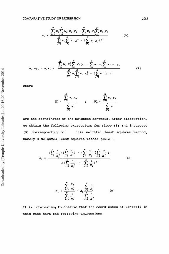
are the coordinates of the weighted centroid. After elaboration,
we obtain the following expressions for slope (8) and intercept
(9) corresponding to this weighted least squares method,
namely X weighted least squares method (XWLS).
It is interesting to observe that the coordinates of centroid in
this case have the following expressions
Dow
nloa
ded
by [
Tem
ple
Uni
vers
ity L
ibra
ries
] at
20:
16 2
0 N
ovem
ber
2014

2084
and will be much more close to the origin comparative with
ordinary least squares method. Moreover, the standard deviations
of slope and intercept calculated with equation (10) and (11)
respectively, will be also much smaller applying this more
general approach.
I Y
In the last two equations s represents the standard deviation of
residuals and it was calculated as usual using weighted
regression.
RESULTS AND DISCUSSION
Computing the relevant examples of heteroscedasticity
discussed by Garden and all9, using the inverse of variance as a
weighting factor (wi = l /s i2) (case l), and Miller and Miller’
(case 2) which used wi = si-’(Zsi-’/n) we obtained the results
presented in Table 1. The case 3 and 4 shown also in Table 1
refer to the data computing by Phillips and Eyringg to illustrate
Dow
nloa
ded
by [
Tem
ple
Uni
vers
ity L
ibra
ries
] at
20:
16 2
0 N
ovem
ber
2014

COMPARATIVE STUDY OF REGRESSION 2085
the insensitivity of the technique of iteratively reweighted
least squares (IRLS) to erroneous observations (case 3 ) and the
case 4 , respectively compare the results given by XWLS with the
results reported by Aarons” using OLS, WLS and an extended least
squares method (ELS) to study the reproducibility for ibuprofen
assay. Considering the results (see Table 1) and taking into
account the major disavantage of the WLS and ELS method, namely
difficulty of obtaining a good estimate of variance and the
computation for ELS and IRLS the XWLS method appears to be the
most suitable. The performance of XWLS exceeds that of
coventional ordinary least squares method and equals or often
exceeds that of weighted and robust regression.
To illustrate the characteristics of performance ofthe XWLS
method in the situations of small deviations from
homoscedasticity or in presence of outliers, we refer to the data
discussed by Rajk6’ concerning the determination of Mo, Cr, Co,
Pb and Ni in sub-surface and drinking water by ICP-AES (Table 2).
Considering the results obtained (Table 3 ) using eight different
calibration methods namely, ordinary least squares (LS), least
sum of absolute residuals (LSA), least maximum absolute residuals
(LMA), iteratively reweighted least squares with tuning constants
6 and 9 (IRLS6 and IRLS9), most frequent values (MFV), single
median (SM) , repeated median (RM) , least median of squares (LMS) , Rajkb concluded that the best results were given by LMS. MFV
yielded appropriate results for measurements of Mo, Cr, Pb, Co and
Ni(221.6 nm). The calibration line calculated by RM was
acceptable for Cr, Pb and Ni measured at both wavelengths, and
by IRLS6 for Mo and Co. SM was good for Pb and Ni(231.6 nm) and
LSA for only Mo. IRLS9 and LS gave nearly the same results. LMA
Dow
nloa
ded
by [
Tem
ple
Uni
vers
ity L
ibra
ries
] at
20:
16 2
0 N
ovem
ber
2014

2086 sAmu
Table 1. Comparison of conventional ordinary least squares (OLS),
weighted least squares method (WLS), iteratively reweighted least
squares (IRLS) and an extended weighted least squares (ELS) with
X weighted least squares method (XWLS) computing data sets
from2,9,19.20.
................................................................. Method Case 1 Case 2 Case 3 Case 4
OLS
WLS
IRLS
ELS
XWLS
a0 0.15 0.0091
a0 a1
a0 a1
a1 0.95 0.0738
0.19 0.92
a0 0.01 0.0090 -0.04 0.98 0.0737 1.09
0.0057 0.0199
0.0072 0.0197
0.0073 0.0196
Table 2. Calibration data measured by ICP-AES
Dow
nloa
ded
by [
Tem
ple
Uni
vers
ity L
ibra
ries
] at
20:
16 2
0 N
ovem
ber
2014

COMPARATIVE STUDY OF REGRESSION 2087
Table 3. Estimated parameters obtained by the methods mentioned
in the text for the data in Table 2
................................................................. Method Mo Cr co Pb Ni* Ni**
LS a, -3.1 -11.9 17.2 9.8 0.5 21.9 al 814.5 858.5 846.1 413.0 886.3 798.7
al 802.5 845.6 859.0 407.1 884.1 807.1 LMA a, -6.3 -12.8 21.7 8.7 -3.4 19.8
.................................................................
LSA a, 8.2 -2.4 1.3 13.5 2.7 19.0
al 802.1 864.0 862.1 412.7 889.8 797.7 IRLS6 a, 11.1 -11.7 -1.5 10.0 0.9 22.2
IRLS9 a, -1.9 -11.8 15.7 9.9 0.6 22.0 al 802.3 858.0 862.1 412.9 885.8 799.1
al 813.6 858.3 847.2 412.9 886.1 798.8 MFV a, 9.4 1.3 -2.0 10.3 6.4 22.9
al 803.9 840.8 862.1 412.1 880.4 801.3 SM a, 5.3 -9.2 0.4 9.7 5.1 26.7
al 808.4 854.6 860.2 412.9 880.0 782.7 RM a, 2.1 -1.6 2.3 10.4 6.2 28.9
al 813.5 844.5 857.7 410.8 870.9 765.2 LMS a, 12.1 2.4 -1.3 11.8 9.0 29.4
al 802.5 839.6 862.0 407.1 848.6 761.1 XWLS a, 12.1 -21.4 -2.1 9.9 6.9 29.4
al 751.7 894.8 926.6 413.9 863.6 772.7
al 836.2 852.9 857.0 412.7 872.1 799.0 WLS a, -19.6 -7.8 5.0 10.3 6.7 22.0
____________________-------------------------------------------- *measured at wavelength 221.6 nm measured at wavelength 231.6 nm * *
gave very biased parameters, in fact it was the most sensitive
to the outliers.
Comparing the results obtained by computation of the XWLS
method, presented also in Table 3, it is easy to observe that the
XWLS is more closer to the LMS. Much more in the same table were
enclosed the results obtained by ordinary weighted least squares
method (WLS) using the reciprocal of variances as weighting
factors. The variances were calculated only for two replicates
available in the data of Rajk6 and are shown in Table 4.
Concerning the WLS we remark good results for Co, Pb,
Ni(221.6mn), especially in the cases of heteroscedasticity (see
si2 in Table 4).
Dow
nloa
ded
by [
Tem
ple
Uni
vers
ity L
ibra
ries
] at
20:
16 2
0 N
ovem
ber
2014

2088 sARBu
In addition, for a more realistic comparison of the ten
methods of regression presented in Table 3 , we calculated the
estimates of sample concentration considering two values of the
signal y, 100 and 600, respectively. A careful examination of
results presented in Table 5 illustrates that the performance of
the XWLS equals that of LMS in some cases, and exceeds some of
the other methods.
A high discrepancy appears, however, for Mo and Co at 600
arbitrary units and also for Cr at 100 units. These results
confirm one more time that weighted methods provide, generally,
more accurate estimates of unknown samples at lower
concentration, and introduce the question if the LMS method is
realy the best in all these cases (see also Table 7 and 8).
As we have emphasized above the weighted centroid (%,:J is
much closer to the origin of the graph than the unweighted
centroid (x,y), and the weighting given the points nearer the origin - and particularly to the first point, which has the smallest error - ensures that the weighted regression line has an intercept very close to the first point (see Table 6).
Moreover, the weighted regression gives a smaller standard error,
which is more appropriate and allows us to detect a smaller bias
in the intercept that isreally present. These conclusions are
well illustrated in Table 6 .
Dow
nloa
ded
by [
Tem
ple
Uni
vers
ity L
ibra
ries
] at
20:
16 2
0 N
ovem
ber
2014

COMPARATIVE STUDY OF REGRESSION 2089
Table 5. The estimated concentrations corresponding to 100 and
600 signal value, respectively obtained by each method
in Table 3.
................................................................ Method Mo Cr co Pb Ni* Ni,,
100 100 100 100 100 100 ................................................................ LS 0.123 0.130 0.098 0.218 0.112 0.098 LSA 0.114 0.121 0.115 0.213 0.110 0.100 LMA 0.133 0.131 0.091 0.221 0.116 0.101 IRLS6 0.111 0.130 0.118 0.218 0.112 0.097 IRLS9 0.125 0.130 0.100 0.218 0.112 0.098 MFV 0.113 0.117 0.118 0.218 0.106 0.096 SM 0.117 0.128 0.117 0.219 0.108 0.094 RM 0.121 0.120 0.114 0.218 0.108 0.093 LMS 0.110 0.116 0.118 0.217 0.107 0.093 XWLS 0.117 0.136 0.110 0.218 0.108 0.091 WLS 0.143 0.138 0.111 0.217 0.107 0.098 ................................................................
600 600 600 600 600 600 ........................................................ LS 0.740 0.713 0.689 1.429 0.676 0.724 LSA 0.737 0.712 0.697 1.441 0.676 0.719 LMA 0.756 0.709 0.671 1.433 0.678 0.727 IRLS6 0.734 0.713 0.698 1.429 0.676 0.723 IRLS9 0.740 0.713 0.690 1.429 0.676 0.724 MFV 0.735 0.712 0.698 1.430 0.674 0.720 SM 0.736 0.713 0.697 1.430 0.676 0.733 RM 0.735 0.712 0.697 1.435 0.682 0.746 LMS 0.733 0.712 0.698 1.445 0.697 0.750 XWLS 0.782 0.700 0.690 1.436 0.687 0.739 WLS 0.741 0.724 0.694 1.429 0.680 0.723 ___-____________________________________------------------------- *measured at wavelength 221.6 nm measured at wavelength 231.6 nm * *
Table 6. Estimated standard deviations of intercept, s,,, and
slope, sal, obtained by OLS, XWLS and WLS and the
coordinates of centroid (k,Fw) in the case of XWLS.
................................................................. Method Mo Cr co Pb Ni* Ni**
OLS S,, 9.66 4.83 12.22 3.03 4.68 5.08 *sal 16.87 8.43 21.32 5.28 8.18 8.86
sal 7.20 3.60 9.10 2.26 3.49 3.78 WLS Sao 7.62 3.31 8.62 1.96 3.71 3.28
sal 22.84 9.37 22.62 5.50 29.19 8.79 1.00 1.00 1.00 1.00 1.00 1.00
-2.14 9.93 6.93 29.45 yw 12.12 -21.40
-_________-_____________________________------------------------
XWLS s,, 14.41 7.20 18.21 4.51 6.98 7.57
* x w __---___________________________________------------------------- *x 10-6
Dow
nloa
ded
by [
Tem
ple
Uni
vers
ity L
ibra
ries
] at
20:
16 2
0 N
ovem
ber
2014

2090 sARBu
Referring to the results shown in Table 6 it is interesting
to observe that the coordinates of the centroid are the
coordinates of the first point in the graph. The value 1 ~ 1 0 - ~ of
is due to the replacing of 0 with 1x10 -5 for x to working the -
program.
To evaluate the linearity of the methods studied, it is a
good opportunity to compare the different quality coefficients
(QC) used in the analytical literature to judge the goodness of
fit of a regression line. In this order we present in Table 7 the
values obtained for QC, (12), defined as’,
where yi and pi are the responses measured at each datum and
those predicted by the model in Table 3 , respectively and N is
the number of all data points, QC, used by when measured, yi,
replace estimates pi at the denominator”, and also QC, and QC,,
respectively referring to the mean signalz3 instead of the
signal itself and the mean of estimated signal 9 , respectively. The smaller the QC, the better the fit of the model.
The main conclusion drawn from the results in Table 7 by
comparing with the statements of Rajk6’ is that QC, and QC,,
respectively are most suitable to evaluate the goodness of fit
at least for the data computed in this paper. The quality
coefficient QC, and QC,, respectively appear to be a better
solution when comparing methods based on the same algorithm, i.e.
least squares. Rajk6 appreciated the QC, criterion as a pleasant
solution but he has not used it in his paper.
Taking into account the contradictory values of QC and the
diversity of the methods concerning their algorithm we have
Dow
nloa
ded
by [
Tem
ple
Uni
vers
ity L
ibra
ries
] at
20:
16 2
0 N
ovem
ber
2014

COMPARATIVE STUDY OF REGRESSION 209 1
LS LSA LMA IRLS6 IRLS9 MFV SM RM LMS XWLS LS LSA LMA IRLS6 IRLS9 MFV SM RM LMS XWLS LS LSA LMA IRLS6 IRLS9 MFW SM RM LMS XWLS LS LSA LMA IRLS6 IRLS9 MFV SM RM LMS XWLS
QCl
QC2
QC3
QC4
273.4 37.2
160.1 21.5
413.5 28.8 81.0
288.5 19.7 19.2 69.2 21.1 85.3 20.9 63.3 19.7 30.4 44.6 23.2 22.1 4.6 5.1 5.6 5.4 4 . 6 5.2 4.9 4.8 5.5 9.2 4.6 5.1 5.5 5.5 4.6 5.3 5.0 4.8 5.7 9.5
43.4 425.5 36.9 45.3 44.5
930.2 72.5 688.0 531.9
6.0 23.7 47.4 21.5 24.3 24.0 56.8 30.5 49.6 59.5 6.0 2.3 2.9 2.4 2.2 2.2 3.3 2.3 3.0 3.5 4.9 2.3 2.9 2.4 2.2 2.2 3.4 2.3 3.0 3.5 4.8
60.6 142.4 59.0 30.2 61.9 15.3
349.5 105.1 36.1 11.8
497.1 87.2
612.4 19.8
457.7 12.6 64.1
115.3 22.1 11.6 5.3 6.3 6.2 6.6 5.4 6.7 6.4 6.3 6.4
10.7 5.3 6.2 6.4 6.4 6.4 6.5 6.3 6.1 6.4
10.3
19.4 20.0 23.1 19.1 19.2 18.6 19.8 18.5
19.2 22.9 42.0 19.3 23.5 23.1 24.8 22.1 25.3 32.3 23.2 2.7 3.0 2.8 2.7 2.7 2.7 2.7 2.7 3.0 2.7 2.7 3.0 2.8 2.7 2.7 2.7 2.7 2.7 3.0 2.7
18.3
735.5 86.1
163.7 384.1 536.9
6.8 20.2 8.1
4.6 49.8 32.9 79.6 46.9 48.6 6.0
14.4 6.8
17.2 4.6 2.0 2.1 2.2 2.0 2.0 2.3 2.2 2.6 4.9 3.2 2.0 2.1 2.2 2.0 2.0 2.3 2.2 2.6 4.9 3.3
12.8
18.6 29.6 26.2 17.7 18.4 15.6 6.2 3.2
3.2 2.9
13.8 19.0 17.6 13.3 13.7 12.1 5.5 3.1 3.1 2.6 2.3 2.5 2.4 2.3 2.3 2.4 3.0 4.9 5.3 3.8 2.3 2.9 2.4 2.3 2.3 2.4 2.9 4.8 5.3 3.8 ________________________________________-------------------------
*measured at wavelength 221.6 nm measured at wavelength 231.6 nm **
Dow
nloa
ded
by [
Tem
ple
Uni
vers
ity L
ibra
ries
] at
20:
16 2
0 N
ovem
ber
2014

2092 sAmu
introduced two new quality coefficients namely QC, and QC,
respectively referring to the maximum of absolute residuals
(mad rd ) and the mean of the absolute residuals, ri,
respectively at the denominator in Equation 12. The results
obtained by computing QC, and QC,, respectively are shown in
Table 8. It is easy to observe a very good agreement of the
values in Table 8 with the Rajk6 statements especially for QC,.
Overall, it may be stated that these new quality coefficients
concerning the goodness of fit proposed in this paper confirm our
main conclusions and are in a good agreement with the statements
in the analytical literature.
We have to remark that in the case of QC, the higher the QC
values the better the fit of the model.
Moreover, the QC, criterion appears to be really a pleasant
solution because it is more sensitive and reliable and takes
values approximately within 1 and 2 (without multiplication by
100).
CONCLUSIONS
The weighted least squares method ( X W L S ) compared in this
paper uses the inverse of square of X i , namely 1 / X i 2 , as a
weighting factor in linear regression analysis. Given the present
results and many others computed by the author and unpublished,
it seems that the XWLS method is the best one for dealing
with problems of heteroscedasticity. The XWLS method produces
accurate and precise estimates of the parameters of calibration
line and is efficient over a broad range of error distributions.
The performance of XWLS has been shown to exceed that of
conventional ordinary least squares method and equals or often
exceeds that of weighted and robust regression. The method is
Dow
nloa
ded
by [
Tem
ple
Uni
vers
ity L
ibra
ries
] at
20:
16 2
0 N
ovem
ber
2014
COMPARATIVE STUDY OF REGRESSION 2093
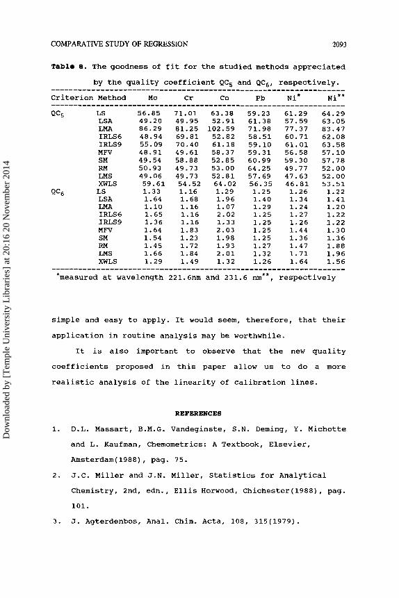
Table 8. The goodness of fit for the studied methods appreciated
by the quality coefficient QC, and QC,, respectively. ................................................................. Criterion Method Mo Cr co Pb Ni Ni** .................................................................
LS 56.85 71.01 63.38 59.23 61.29 64.29 LSA 49.20 49.95 52.91 61.38 57.59 63.05 LMA 86.29 81.25 102.59 71.98 77.37 83.47 IRLS6 48.94 69.81 52.82 58.51 60.71 62.08 IRLS9 55.09 70.40 61.18 59.10 61.01 63.58 MFV 48.91 49.61 58.37 59.31 56.58 57.10 SM 49.54 58.88 52.85 60.99 59.30 57.78 RM 50.93 49.73 53.00 64.25 49.77 52.00 LMS 49.06 49.73 52.81 57.69 47.63 52.00 XWLS 59.61 54.52 64.02 56.35 46.81 53.51 LS 1.33 1.16 1.29 1.25 1.26 1.22 LSA 1.64 1.68 1.96 1.40 1.34 1.41 LMA 1.10 1.16 1.07 1.29 1.24 1.20 IRLS6 1.65 1.16 2.02 1.25 1.27 1.22 IRLS9 1.36 1.16 1.33 1.25 1.26 1.22 MFV 1.64 1.83 2.03 1.25 1.44 1.30 SM 1.54 1.23 1.98 1.25 1.36 1.36 RM 1.45 1.72 1.93 1.27 1.47 1.88 LMS 1.66 1.84 2.01 1.32 1.71 1.96 XWLS 1.29 1.49 1.32 1.26 1.64 1.56
QC5
Qc6
................................................................. *measured at wavelength 221.6nm and 231.6 nm**, respectively
simple and easy to apply. It would seem, therefore, that their
application in routine analysis may be worthwhile.
It is also important to observe that the new quality
coefficients proposed in this paper allow us to do a more
realistic analysis of the linearity of calibration lines.
1.
2.
3 .
REFERENCES
D.L. Massart, B.M.G. Vandeginste, S.N. Deming, Y. Michotte
and L. Kaufman, Chemometrics: A Textbook, Elsevier,
Amsterdam(l988), pag. 75.
J.C. Miller and J.N. Miller, Statistics for Analytical
Chemistry, 2nd, edn., Ellis Horwood, Chichester(l988), pag.
101.
J. Agterdenbos, Anal. Chim. Acta, 108, 315(1979).
Dow
nloa
ded
by [
Tem
ple
Uni
vers
ity L
ibra
ries
] at
20:
16 2
0 N
ovem
ber
2014

2094 sAmu
4.
5.
6.
7.
8.
9.
10.
11.
12.
13.
14.
15.
16.
17.
18.
19.
20.
21.
22.
23.
J. Agterdenbos, Anal. Chim. Acta, 132, 127(1981).
J.N. Miller, Analyst, 116, 3(1991).
G. Klimov, Probability Theory and Mathematical Statistics,
Mir Publishers Moscow(1986), pag. 272.
R. Rajk6, Anal. Lett., 27, 215(1994).
M. Thompson, Analyst, 119, 127N(1994).
G.R. Phillips and E.M. Eyring, Anal. Chem., 55, 1134(1983).
L.M. Schwartz, Anal. Chem., 49, 2062(1977).
L.M. Schwartz, Anal. Chem., 51, 723(1979).
R.C. Rutan, and P.W. Carr, Anal. Chim. Acta, 215, 131(1988).
Y. Hu, J. Smeyers-Verbeke and D.L. Massart, J. Anal. At.
Spectrom., 4, 605(1989).
R. Wolters and G. Kateman, J. Chemom., 3, 329(1989).
P. Vankeerberghen, C. Vandenbosch, J. Smeyers-Verbeke and
D.L. Massart, Chemom. Intell. Lab. Syst., 12, 3(1991).
L. Galan, H.P.J. van Dalen and G.R. Kornblum, Analyst, 110,
323 (1985).
J.N. Miller, Spectroscopy Europe, 5(6), 22(1992).
P.L. Bonate, LC-GC, 10(6), 448(1991).
J.S. Garden, D . S . Mitchell and W.N. Mills, Anal. Chem., 52,
2310(1980).
L. Aarons, J. Pharm. Biomed. Anal., 2, 395(1984).
J. Knegt and G. Stork, Fresenius' 2. Anal. Chem., 270,
97 (1974) . P. KoScielniak, Anal. Chim. Acta, 278, 177(1993).
W. Xiaoning, J. Smeyers-Verbeke, D.L. Massart, Analusis, 20,
209 (1992) .
Receivec!: February I & , 1 0 0 5 Accepted : ?!arch ? P , 1'j01
Dow
nloa
ded
by [
Tem
ple
Uni
vers
ity L
ibra
ries
] at
20:
16 2
0 N
ovem
ber
2014
Recommended