A Combustion Model for

Diesel Engines

FREDRIK KÖNIGSSON

Master of Science Thesis

Stockholm, Sweden 2010

A Combustion Model for Diesel Engines

Fredrik Königsson

Master of Science Thesis MMK 2010:16 MFM133

KTH Industrial Engineering and Management

Machine Design

SE-100 44 STOCKHOLM

Examensarbete MMK 2010:16 MFM133

En Förbränningsmodell för Dieselmotorer

Fredrik Königsson

Godkänt

2010-03-31

Examinator

Hans-Erik Ångström

Handledare

Richard Backman

Uppdragsgivare

AVL SPEAB

Kontaktperson

Richard Backman

Sammanfattning En modern dieselmotor utnyttjar Common-Rail bränsleinsprutning med solenoid- eller piezoelektriskt

aktuerade spridare och multipla insprutningar per förbränning för att erhålla ett önskat utseende på

cylindertryckskurvan.

Användandet av multipla insprutningar per förbränning medför flera möjligheter. En sådan möjlighet

är begränsandet av bullernivån vilket erhålls genom tillsättandet av en liten mängd bränsle tidigt

under cykeln vilket i sin tur minskar den förblandade delen av förbränningen som äger rum då

huvuddelen av bränslet tillsätts. Denna teknik kallas för pilotinsprutning. En annan möjlighet är

införandet av en insprutning sent under cykeln, vilket höjer avgastemperaturen och kan förbättra

responsen under transienter, regenerera partikelfilter eller möjliggöra användning av SCR vid

driftsfall med naturligt låga avgastemperaturer .

De ytterligare frihetsgrader som tekniken medför gör att kalibrering av nya motorer blir en alltmer

komplex och tidskrävande process. Ökad förståelse krävs kring hur olika insprutningsmängder och

tidpunkter påverkar cylindertrycket och därigenom motorns verkningsgrad. För att underlätta och

snabba upp denna process är det önskvärt med en analytisk modell för cylindertrycket. Modellen bör

begagna sig av insprutningsmängd och -tidpunkt som indata och prediktera det resulterande

cylindertryckspåret. En sådan modell kan användas som processmodell vid simulering eller för att,

utifrån ett önskat tryckspår, föreslå mängder och tidpunkter vid kalibrering eller i

realtidsapplikationer då cylindertrycksåterkoppling används. Framtagandet av en dylik modell har

varit syftet med detta projekt.

Resultatet är en snabb modell som predikterar vissa driftsfall med god precision men som kräver

ytterligare utveckling för att till fullo fånga de komplexa fenomen som äger rum i en dieselmotor.

Master of Science Thesis MMK 2010:16 MFM133

A Combustion model for Diesel Engines

Fredrik Königsson

Approved

2010-03-31

Examiner

Hans-Erik Ångström

Supervisor

Richard Backman

Commissioner

AVL SPEAB

Contact person

Richard Backman

Abstract A modern diesel engine uses common rail fuel injection with solenoid or piezoelectric valves with

multiple injections for each combustion event to achieve the desired shape of the cylinder pressure

trace during each engine cycle.

The practice of adding the fuel in multiple injections during each combustion event has several

advantages. One is limiting engine noise by adding a small amount of fuel early during the cycle, thus

reducing the premixed part of the combustion once the bulk of the fuel is injected. This is referred to

as pilot injection. Another possibility is the addition of a late injection which raises the exhaust

temperature which can improve transient response, regenerate particle filters or make possible the

use of SCR when low exhaust temperatures would otherwise render such use impossible.

Since multiple injections provide additional degrees of freedom, which were previously unavailable,

the initial tuning of new engines becomes increasingly complex. New understanding must be

achieved as to how different amounts and timings affect the cylinder pressure trace and hence the

overall efficiency of the engine. To aid in the tuning process an analytical model for the cylinder

pressure is desired. The model would use the timings and amounts of fuel injected as its inputs and

predict the resulting cylinder pressure trace, which then could be used as a plant model for

simulations or inversely predict the amount and phase of each injection at calibration or real-time,

using pressure sensor feedback. The development of such a model has been the focus of this project.

The result is a model that, while providing satisfactory precision on some areas, requires more work

to fully capture the complex processes taking place in a firing diesel engine.

Acknowledgements The author wishes to acknowledge certain people, without the help of which this project had not

been completed.

My first thanks goes out to Richard Backman who has been supervising this project, providing

support, encouragement and giving me his opportunity in the first place.

Jonas Cornelsen has been invaluable in ordering and configuring hardware for the test bed and Per

Öberg, PhD at Linköpings university has been most helpful in answering thermodynamic queries and

providing data from CHEPP.

I also like to thank my examiner Hans Erik Ångström, at the Royal Institute of Technology.

Finally my fellow PhD students at the Internal Combustion Engines division deserve a mention for

answering countless questions, small and large and for providing a pleasant atmosphere to work in.

Any mistakes are my own.

Contents

1 Background ...................................................................................................................................... 1

1.1 The internal combustion engine ............................................................................................. 1

1.2 The Diesel Engine of today ...................................................................................................... 1

1.3 Diesel Combustion ................................................................................................................... 4

1.4 Diesel fuel ................................................................................................................................ 6

1.5 Combustion Modelling ............................................................................................................ 7

1.5.1 Single Zone ...................................................................................................................... 7

1.5.2 Multi Zone ....................................................................................................................... 8

1.5.3 Multi dimensional ............................................................................................................ 8

2 The model ........................................................................................................................................ 9

2.1 Overview .................................................................................................................................. 9

2.2 Initiation ................................................................................................................................ 10

2.3 Gas Exchange ......................................................................................................................... 11

2.4 Compression .......................................................................................................................... 12

2.5 Expansion .............................................................................................................................. 13

2.6 Specific Heat Ratio ................................................................................................................. 13

2.6.1 A constant throughout the compression and expansion stroke. ............................... 14

2.6.2 A that changes linearly as a function of mean charge temperature, . .................... 14

2.6.3 A modeled as a polynomial in , , and . ................................................................ 14

2.6.4 Assuming that the unburned mixture is frozen and that the burned mixture is at

chemical equilibrium at every instant. .......................................................................... 15

2.6.5 Chosen concept ............................................................................................................. 16

2.7 Fuel Injection ......................................................................................................................... 18

2.8 Ignition delay ......................................................................................................................... 19

2.9 Fuel Evaporation .................................................................................................................... 21

2.10 Combustion ........................................................................................................................... 22

2.11 Heat Transfer ......................................................................................................................... 24

3 Validation ...................................................................................................................................... 25

3.1 Experimental setup ............................................................................................................... 25

3.2 Measurements ...................................................................................................................... 26

3.3 Compression .......................................................................................................................... 26

3.4 Expansion .............................................................................................................................. 31

3.5 Specific heat ratio .................................................................................................................. 32

3.6 Fuel Injection ......................................................................................................................... 35

3.7 Fuel preparation and Combustion ........................................................................................ 36

3.8 Ignition delay ......................................................................................................................... 40

3.9 Heat Transfer ......................................................................................................................... 42

3.10 Closed Cycle ........................................................................................................................... 43

4 Conclusions .................................................................................................................................... 47

4.1 Future work ........................................................................................................................... 47

5 References: .................................................................................................................................... 48

6 Abbreviations ................................................................................................................................ 49

Appendix A: Constants .......................................................................................................................... 50

1

1 Background

1.1 The internal combustion engine For the past 300 years man has wrestled with the task of converting chemical energy stored in

various fuels into useful work. The first solution to this problem that saw widespread use was the

steam engine. Originally used to evacuate water from the coal mines of England, the steam engine

went on to become the power plant of choice and a driving factor during the industrial revolution.

The steam engine is an external combustion engine, where the combustion takes place outside the

cylinder or the turbine, and a different medium, in this case water vapor, is used to transfer the

work. This stands in contrast to the internal combustion engine, where the fuel-air mixture and the

residual gases are the actual working fluids that transfer the work to the piston. However, it took an

additional century and a half until engines based on this principle became a working alternative.

In 1860 the first practical internal combustion engines became available. Burning a mixture of coal-

gas and air without compression, attaining an efficiency of 5%, these early engines were

manufactured in relatively small numbers. It was not until 1876, when Nicolaus A. Otto ran his first

four-stroke engine, that the internal combustion engine got the breakthrough needed to become the

predominant power source that it is today. [1]

Recognizing that the greater the expansion of the post combustion gases, the greater the work

transferred, attempts were made to increase the expansion ratio. Continuing on the theoretical work

of Alphonse Beau de Rochas, James Atkinson constructed an engine where the expansion stroke was

longer than the compression stroke. His engine, however, was plagued by mechanical problems and

this course of action was more or less abandoned. Therefore for the next hundred year’s expansion

and compression ratios have been linked and the desire to increase the expansion ratio translates

into a need to increase the compression ratio.

The fuels available at the time did not permit compression ratios larger than 4 before the onset of

knock, and while improvements were made to carburetors and ignition systems to help address this

problem, Rudolf Diesel proposed a different approach. [1] In his patent from 1890 he outlined a new

type of combustion engine where the fuel was not added until after the compression and the

temperature of the hot compressed air was sufficient to ignite the fuel. Rudolf Diesel improved on

the concept by further increasing the compression ratio, and due to his success in patenting his

ideas, he is generally considered the inventor of the engine that bears his name. This new concept,

the diesel engine, would permit much greater expansion ratios and thus greater efficiency. Since

then, for the past hundred years, wars, economic interests and lately emissions legislation have

driven the development of the diesel engine into its current form. Advances has been made in many

fields; from the materials used, casting methods and engine geometry, to strategies for injection

timings, and the software used for engine control.

1.2 The Diesel Engine of today Today the Diesel engine is used throughout the world in various applications, from two stroke ship

engines where each pistons displacement is measured in cubic meters to lightweight high speed

engines running at 10000 RPM used in reconnaissance planes. The work presented in this thesis is

2

aimed towards automotive applications and more specifically heavy duty truck engines. These are

four stroke reciprocating engines, where the piston moves back and forth in the cylinder between

bottom dead center, BDC, and top dead center, TDC, firing once every 720 degrees. This means that

four strokes of the piston is required for each power generating stroke, and hence the name four

stroke engine.

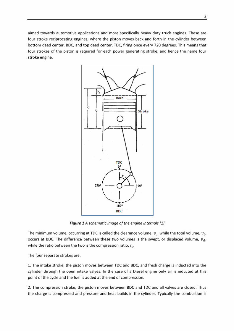
Figure 1 A schematic image of the engine internals [1]

The minimum volume, occurring at TDC is called the clearance volume, , while the total volume, ,

occurs at BDC. The difference between these two volumes is the swept, or displaced volume, ,

while the ratio between the two is the compression ratio, .

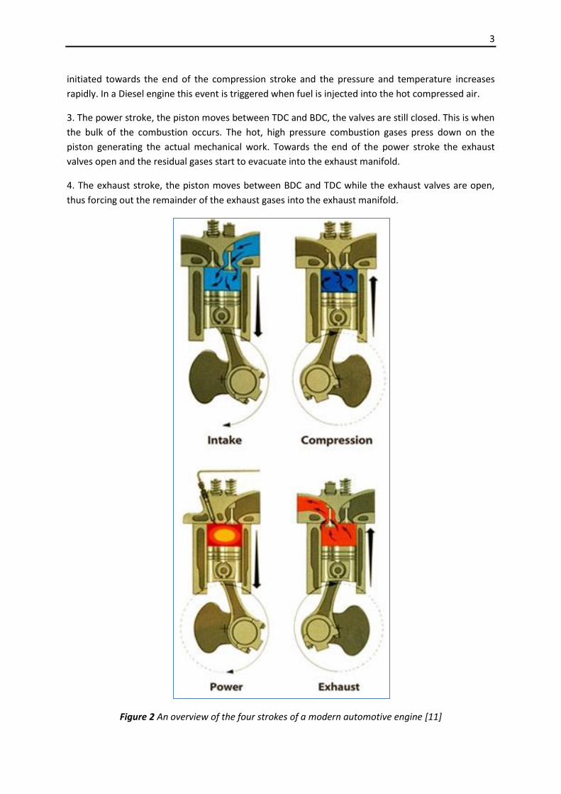
The four separate strokes are:

1. The intake stroke, the piston moves between TDC and BDC, and fresh charge is inducted into the

cylinder through the open intake valves. In the case of a Diesel engine only air is inducted at this

point of the cycle and the fuel is added at the end of compression.

2. The compression stroke, the piston moves between BDC and TDC and all valves are closed. Thus

the charge is compressed and pressure and heat builds in the cylinder. Typically the combustion is

3

initiated towards the end of the compression stroke and the pressure and temperature increases

rapidly. In a Diesel engine this event is triggered when fuel is injected into the hot compressed air.

3. The power stroke, the piston moves between TDC and BDC, the valves are still closed. This is when

the bulk of the combustion occurs. The hot, high pressure combustion gases press down on the

piston generating the actual mechanical work. Towards the end of the power stroke the exhaust

valves open and the residual gases start to evacuate into the exhaust manifold.

4. The exhaust stroke, the piston moves between BDC and TDC while the exhaust valves are open,

thus forcing out the remainder of the exhaust gases into the exhaust manifold.

Figure 2 An overview of the four strokes of a modern automotive engine [11]

4

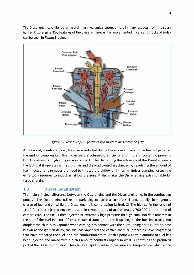
The Diesel engine, while featuring a similar mechanical setup, differs in many aspects from the spark

ignited Otto engine. Key features of the diesel engine, as it is implemented in cars and trucks of today

can be seen in Figure 3 below.

Figure 3 Overview of key features in a modern diesel engine [10]

As previously mentioned, only fresh air is inducted during the intake stroke and the fuel is injected at

the end of compression. This increases the volumetric efficiency and, more importantly, prevents

knock problems at high compression ratios. Further benefiting the efficiency of the Diesel engine is

the fact that it operates with surplus air and the load control is achieved by regulating the amount of

fuel injected, this removes the need to throttle the airflow and thus minimizes pumping losses, the

extra work required to induct air at low pressure. It also makes the Diesel engine extra suitable for

turbo charging.

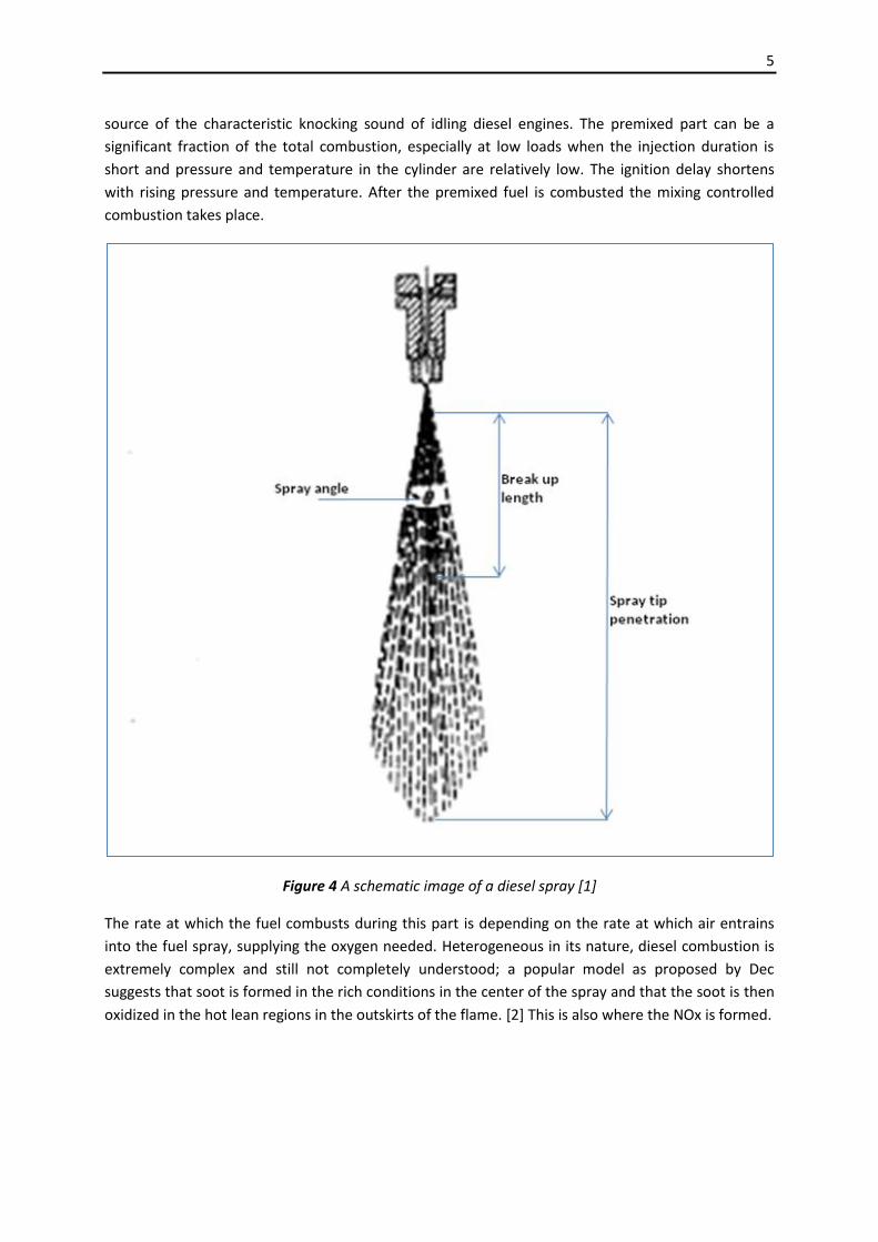
1.3 Diesel Combustion The main principal difference between the Otto engine and the Diesel engine lies in the combustion

process. The Otto engine utilizes a spark plug to ignite a compressed and, usually, homogenous

charge of fuel and air while the Diesel engine is compression ignited, CI. The high , in the range of

16-19 for direct injected engines, results in temperatures of approximately 700-900 C at the end of

compression. The fuel is then injected at extremely high pressure through small nozzle diameters in

the tip of the fuel injector. After a certain distance, the break up length, the fuel jet breaks into

droplets which in turn vaporize when coming into contact with the surrounding hot air. After a time

known as the ignition delay, the fuel has vaporized and certain chemical processes have progressed

that have prepared the fuel, and the combustion starts. At this point a certain amount of fuel has

been injected and mixed with air, this amount combusts rapidly in what is known as the premixed

part of the Diesel combustion. This causes a rapid increase in pressure and temperature, which is the

5

source of the characteristic knocking sound of idling diesel engines. The premixed part can be a

significant fraction of the total combustion, especially at low loads when the injection duration is

short and pressure and temperature in the cylinder are relatively low. The ignition delay shortens

with rising pressure and temperature. After the premixed fuel is combusted the mixing controlled

combustion takes place.

Figure 4 A schematic image of a diesel spray [1]

The rate at which the fuel combusts during this part is depending on the rate at which air entrains

into the fuel spray, supplying the oxygen needed. Heterogeneous in its nature, diesel combustion is

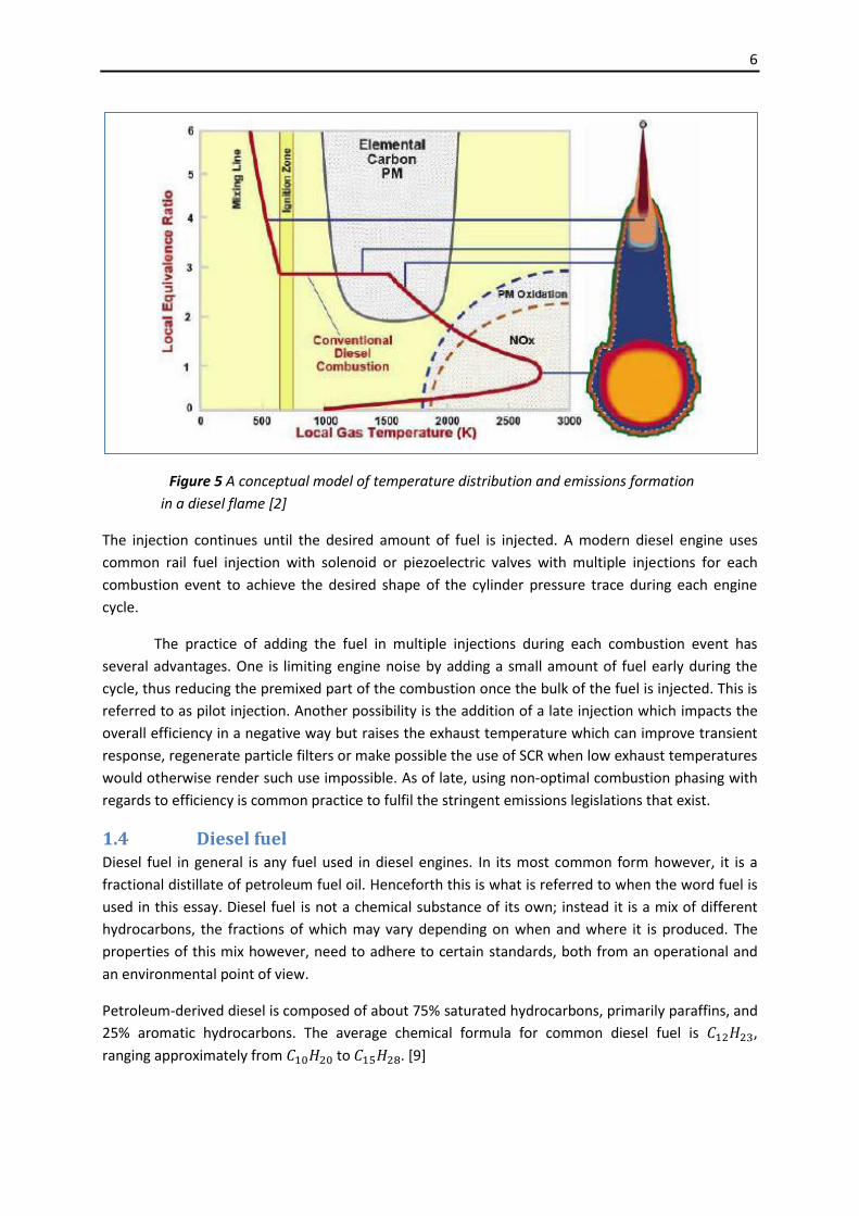
extremely complex and still not completely understood; a popular model as proposed by Dec

suggests that soot is formed in the rich conditions in the center of the spray and that the soot is then

oxidized in the hot lean regions in the outskirts of the flame. [2] This is also where the NOx is formed.

6

Figure 5 A conceptual model of temperature distribution and emissions formation

in a diesel flame [2]

The injection continues until the desired amount of fuel is injected. A modern diesel engine uses

common rail fuel injection with solenoid or piezoelectric valves with multiple injections for each

combustion event to achieve the desired shape of the cylinder pressure trace during each engine

cycle.

The practice of adding the fuel in multiple injections during each combustion event has

several advantages. One is limiting engine noise by adding a small amount of fuel early during the

cycle, thus reducing the premixed part of the combustion once the bulk of the fuel is injected. This is

referred to as pilot injection. Another possibility is the addition of a late injection which impacts the

overall efficiency in a negative way but raises the exhaust temperature which can improve transient

response, regenerate particle filters or make possible the use of SCR when low exhaust temperatures

would otherwise render such use impossible. As of late, using non-optimal combustion phasing with

regards to efficiency is common practice to fulfil the stringent emissions legislations that exist.

1.4 Diesel fuel Diesel fuel in general is any fuel used in diesel engines. In its most common form however, it is a

fractional distillate of petroleum fuel oil. Henceforth this is what is referred to when the word fuel is

used in this essay. Diesel fuel is not a chemical substance of its own; instead it is a mix of different

hydrocarbons, the fractions of which may vary depending on when and where it is produced. The

properties of this mix however, need to adhere to certain standards, both from an operational and

an environmental point of view.

Petroleum-derived diesel is composed of about 75% saturated hydrocarbons, primarily paraffins, and

25% aromatic hydrocarbons. The average chemical formula for common diesel fuel is ,

ranging approximately from to . [9]

7

Important qualities when discussing fuels from an engine point of view is ignition quality, heat of

vaporization, density, heating value, air to fuel ratio, volatility, cleanliness and corrosivity. Among

these properties the first five have been accounted for in this model, while the latter three have not.

The autoignition characteristics of the fuel are summarized into what is known as the cetane

number, CN. This number is acquired experimentally by comparing the fuel in question with a

reference fuel in a standardized engine test. A low cetane number means that the fuel does not

autoignite easily and that the ignition delay will be long and vice versa. The scale ranges from 15,

represented by heptamethylnonane (HMN, ), a hydrocarbon with very low ignition qualities,

to 100 which is represented by Cetane (n-hexadecane, ). [2] Standard diesel fuel of today for

automotive applications has a CN of . [8]

A high cetane number is usually desired since a short ignition delay results in a small premixed part of

the combustion which in turn leads to better cold start characteristics, less engine wear, less noise

and smoother engine operation. The most important properties of diesel fuel can be found in Table 1

below.

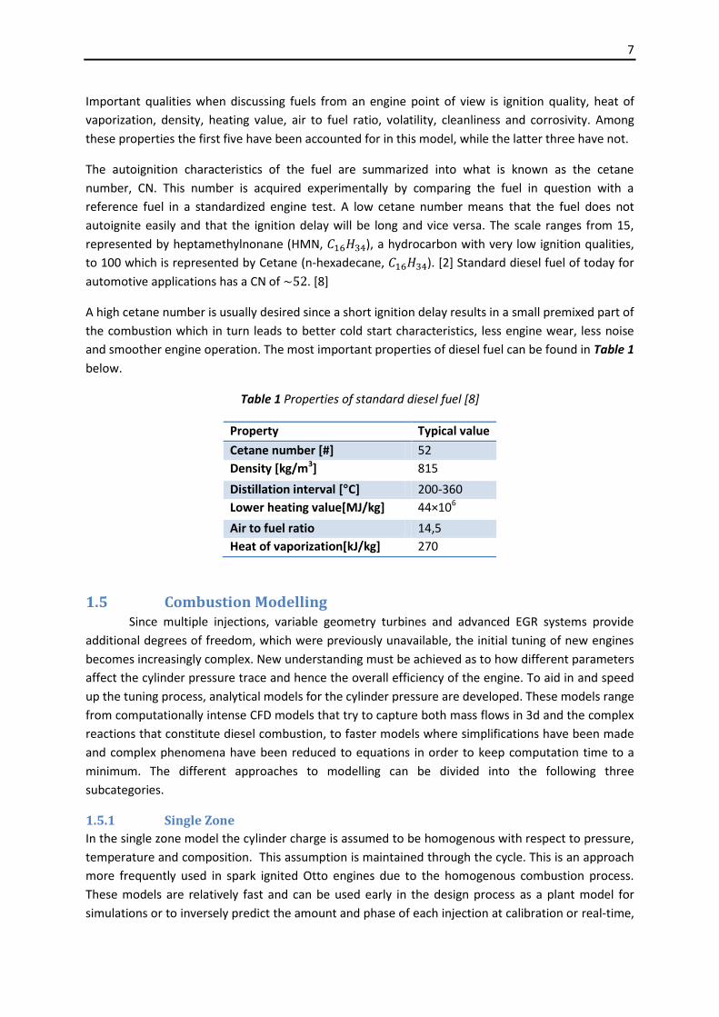
Table 1 Properties of standard diesel fuel [8]

Property Typical value

Cetane number [#] 52

Density [kg/m3] 815

Distillation interval [°C] 200-360

Lower heating value[MJ/kg] 44×106

Air to fuel ratio 14,5

Heat of vaporization[kJ/kg] 270

1.5 Combustion Modelling Since multiple injections, variable geometry turbines and advanced EGR systems provide

additional degrees of freedom, which were previously unavailable, the initial tuning of new engines

becomes increasingly complex. New understanding must be achieved as to how different parameters

affect the cylinder pressure trace and hence the overall efficiency of the engine. To aid in and speed

up the tuning process, analytical models for the cylinder pressure are developed. These models range

from computationally intense CFD models that try to capture both mass flows in 3d and the complex

reactions that constitute diesel combustion, to faster models where simplifications have been made

and complex phenomena have been reduced to equations in order to keep computation time to a

minimum. The different approaches to modelling can be divided into the following three

subcategories.

1.5.1 Single Zone

In the single zone model the cylinder charge is assumed to be homogenous with respect to pressure,

temperature and composition. This assumption is maintained through the cycle. This is an approach

more frequently used in spark ignited Otto engines due to the homogenous combustion process.

These models are relatively fast and can be used early in the design process as a plant model for

simulations or to inversely predict the amount and phase of each injection at calibration or real-time,

8

using pressure sensor feedback. A model of this type is not sufficient for predicting emissions since

local conditions in the flame need to be taken into consideration.

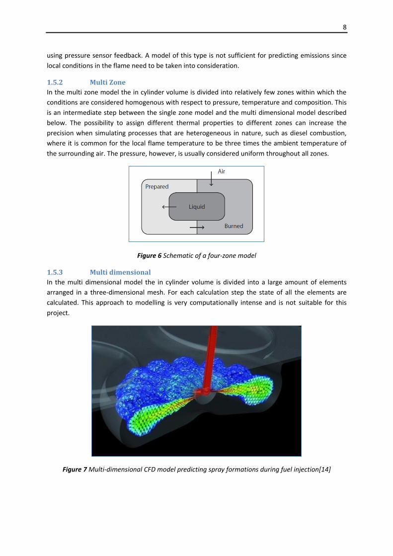
1.5.2 Multi Zone

In the multi zone model the in cylinder volume is divided into relatively few zones within which the

conditions are considered homogenous with respect to pressure, temperature and composition. This

is an intermediate step between the single zone model and the multi dimensional model described

below. The possibility to assign different thermal properties to different zones can increase the

precision when simulating processes that are heterogeneous in nature, such as diesel combustion,

where it is common for the local flame temperature to be three times the ambient temperature of

the surrounding air. The pressure, however, is usually considered uniform throughout all zones.

Figure 6 Schematic of a four-zone model

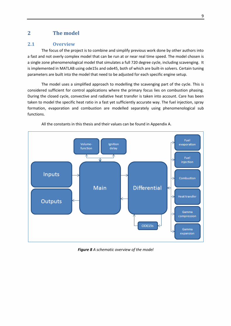
1.5.3 Multi dimensional

In the multi dimensional model the in cylinder volume is divided into a large amount of elements

arranged in a three-dimensional mesh. For each calculation step the state of all the elements are

calculated. This approach to modelling is very computationally intense and is not suitable for this

project.

Figure 7 Multi-dimensional CFD model predicting spray formations during fuel injection[14]

9

2 The model

2.1 Overview The focus of the project is to combine and simplify previous work done by other authors into

a fast and not overly complex model that can be run at or near real time speed. The model chosen is

a single zone phenomenological model that simulates a full 720 degree cycle, including scavenging. It

is implemented in MATLAB using ode15s and ode45, both of which are built-in solvers. Certain tuning

parameters are built into the model that need to be adjusted for each specific engine setup.

The model uses a simplified approach to modelling the scavenging part of the cycle. This is

considered sufficient for control applications where the primary focus lies on combustion phasing.

During the closed cycle, convective and radiative heat transfer is taken into account. Care has been

taken to model the specific heat ratio in a fast yet sufficiently accurate way. The fuel injection, spray

formation, evaporation and combustion are modelled separately using phenomenological sub

functions.

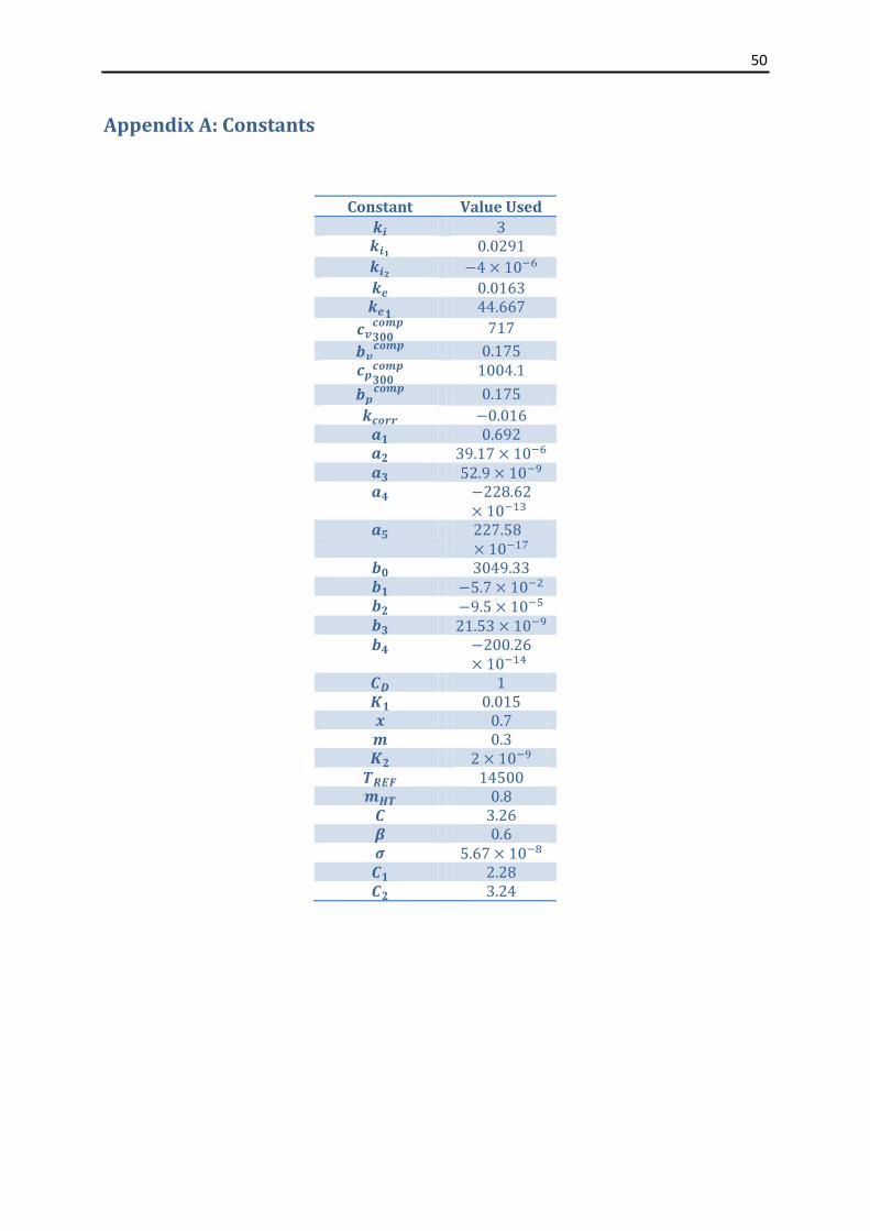
All the constants in this thesis and their values can be found in Appendix A.

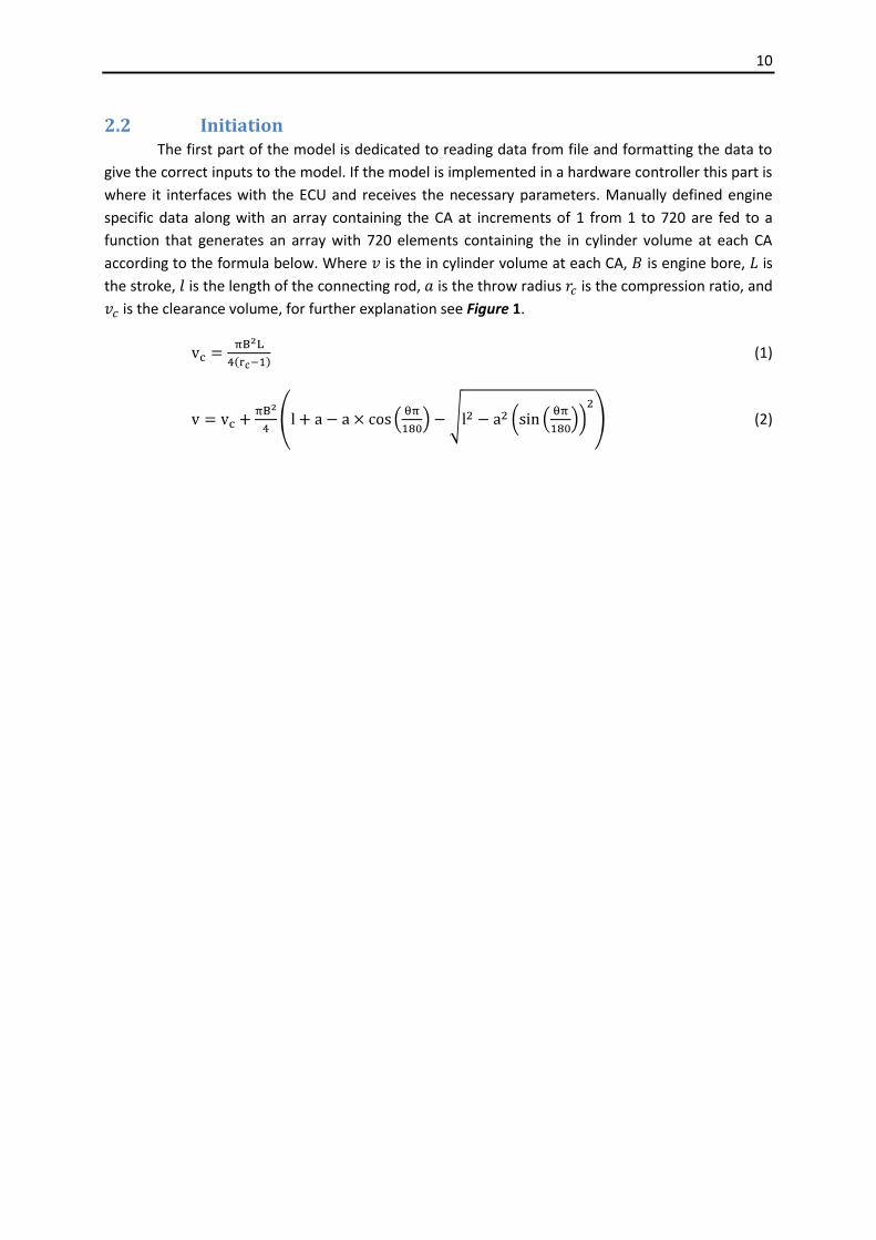
Figure 8 A schematic overview of the model

10

2.2 Initiation The first part of the model is dedicated to reading data from file and formatting the data to

give the correct inputs to the model. If the model is implemented in a hardware controller this part is

where it interfaces with the ECU and receives the necessary parameters. Manually defined engine

specific data along with an array containing the CA at increments of 1 from 1 to 720 are fed to a

function that generates an array with 720 elements containing the in cylinder volume at each CA

according to the formula below. Where is the in cylinder volume at each CA, is engine bore, is

the stroke, is the length of the connecting rod, is the throw radius is the compression ratio, and

is the clearance volume, for further explanation see Figure 1.

(1)

(2)

11

2.3 Gas Exchange The scavenging part of the cycle is modelled using the method proposed in [4], this is a simplified

approach that is sufficient for control applications. Between IVO and IVC the pressure in the cylinder

will be considered equal to the pressure in the inlet manifold, and between EVO and EVC the

pressure is considered equal to the pressure in the exhaust manifold. Predicting the exhaust

backpressure is outside the scope of this thesis, suffice to say it can be modelled or mapped in

advance. For this model, the measured pressure in the exhaust manifold will be used as an input. At

IVO and EVO there is a transition phase, during which the pressure rapidly equalizes across the

valves, this transition phase is depending on the engine speed and is approximated using the method

described below.

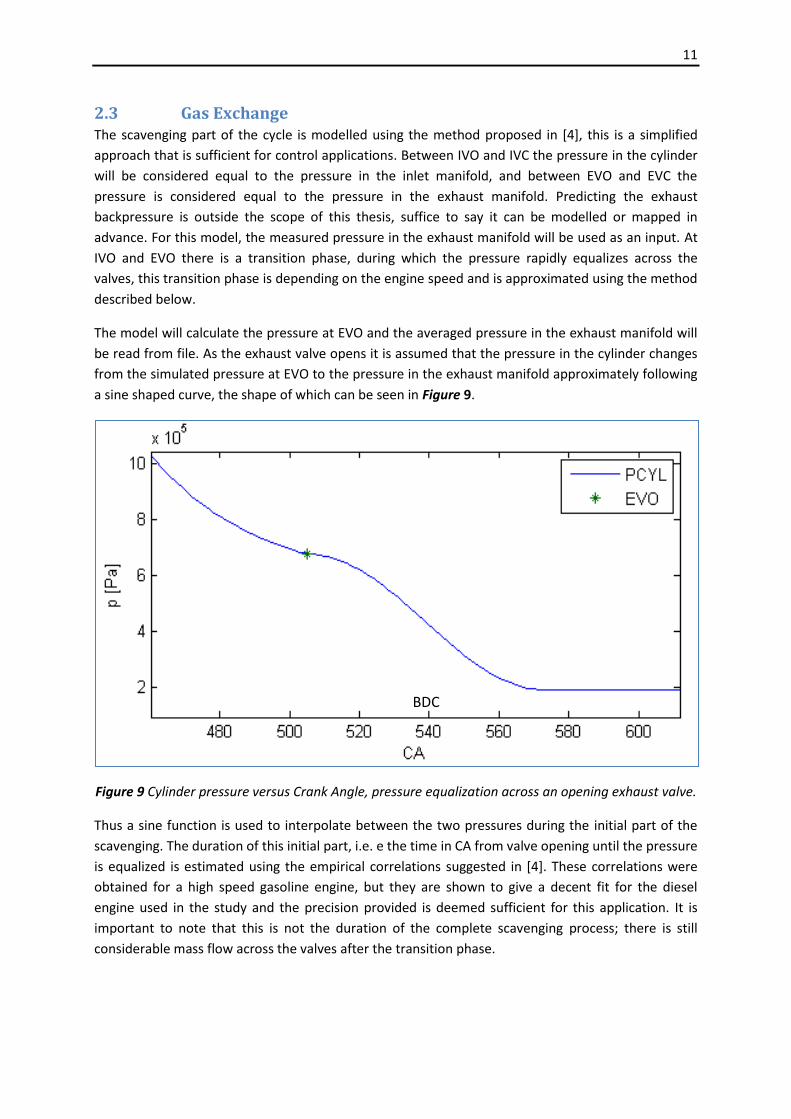
The model will calculate the pressure at EVO and the averaged pressure in the exhaust manifold will

be read from file. As the exhaust valve opens it is assumed that the pressure in the cylinder changes

from the simulated pressure at EVO to the pressure in the exhaust manifold approximately following

a sine shaped curve, the shape of which can be seen in Figure 9.

Figure 9 Cylinder pressure versus Crank Angle, pressure equalization across an opening exhaust valve.

Thus a sine function is used to interpolate between the two pressures during the initial part of the

scavenging. The duration of this initial part, i.e. e the time in CA from valve opening until the pressure

is equalized is estimated using the empirical correlations suggested in [4]. These correlations were

obtained for a high speed gasoline engine, but they are shown to give a decent fit for the diesel

engine used in the study and the precision provided is deemed sufficient for this application. It is

important to note that this is not the duration of the complete scavenging process; there is still

considerable mass flow across the valves after the transition phase.

BDC

12

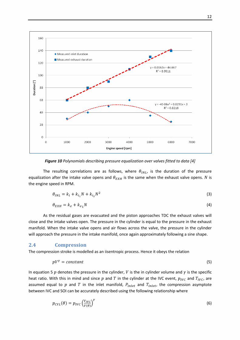
Figure 10 Polynomials describing pressure equalization over valves fitted to data [4]

The resulting correlations are as follows, where , is the duration of the pressure

equalization after the intake valve opens and is the same when the exhaust valve opens. is

the engine speed in RPM.

(3)

(4)

As the residual gases are evacuated and the piston approaches TDC the exhaust valves will

close and the intake valves open. The pressure in the cylinder is equal to the pressure in the exhaust

manifold. When the intake valve opens and air flows across the valve, the pressure in the cylinder

will approach the pressure in the intake manifold, once again approximately following a sine shape.

2.4 Compression The compression stroke is modelled as an iisentropic process. Hence it obeys the relation

(5)

In equation 5 denotes the pressure in the cylinder, is the in cylinder volume and is the specific

heat ratio. With this in mind and since and in the cylinder at the IVC event, and , are

assumed equal to and in the inlet manifold, and , the compression asymptote

between IVC and SOI can be accurately described using the following relationship where

(6)

13

The temperature in the cylinder can be approximated using equation (7).

(7)

As the pressure and temperature increases the thermochemical properties of the gas volume

trapped in the cylinder change. To correctly model the compression using the assumptions above this

problem needs to be addressed. This is done by incorporating a variable that is modeled separately

and changes as the conditions inside the cylinder change. This adds some complexity to the model

and increases calculation time. Additional information on modeling can be found in the section

about specific heat ratio. For the part of the compression stroke when the fuel injection and

combustion have been initiated the equation described in the chapter about the expansion stroke is

used.

The effect of heat transfer during the compression stroke was investigated using the correlations

described in chapter 2.11.

2.5 Expansion The expansion is also modeled in manner similar to the one described above. The specific heat ratio

is modeled using the methods described in chapter 2.6. Equation 6 is rewritten on a different form

permitting release of chemical energy , to be taken into account. This expression has seen

widespread use and the phenomena included are well known. [1] The pressure differential can be

written as

(8)

Where is the crevice volume for the specific engine setup, which is considered zero for this thesis,

hence that part of the expression is neglected.

2.6 Specific Heat Ratio The accuracy with which the compression, combustion and expansion parts of the cycle can be

modeled relies heavily on how accurately one is able to predict the specific heat ratio,

(9)

This ratio is the most influential thermodynamic property used when calculating heat release, and

reversely when modeling pressure change as a result of fuel mass burned. [3] There are several

methods used for calculating when modeling or analyzing combustion, they can all be placed into

one or more of the following subcategories.

14

2.6.1 A constant throughout the compression and expansion stroke.

This is the simplest possible approach, it has the added benefit that the array containing during

compression and expansion can be calculated in a single operation since the array is known.

Common values are during the compression stroke and for the expansion stroke.

However, this method can easily yield large errors and based on the precision of the rest of the

model may be deemed insufficient.

2.6.2 A that changes linearly as a function of mean charge temperature, .

It is assumed that is the only parameter influencing .

(10)

Where and are coefficients that need to be determined. This is a relatively simple and quite

common approach for approximating that was developed by Gatowski et al in 1984. However, the

assumption that changes linearly with is only valid within a relatively narrow temperature range.

When trying to capture large variations in temperature it is either necessary to divide the

temperature range into intervals, each with a separate set of coefficients or to choose a more

complex method. [1] Heywood and Chun propose segmentation into three different segments,

compression, combustion and expansion. Where, during compression and expansion, changes

linearly with , while during combustion a fixed value of is used. This model can be summarized in

the following way:

(11)

Where denotes mass fraction burned, a term more commonly used in association with spark

ignited engines. This model is not continuous however, something which might cause problems in

the transition between the different segments. If the temperature range is large then more segments

can be used to increase the accuracy and the calculation time. In applications where calculation

speed is of high priority or when modeling the compression part of the cycle, the linear method is

popular.

2.6.3 A modeled as a polynomial in , , and .

This is a model with higher complexity than the previous models discussed. The precision and

calculation time depend on the order of the polynomial and how accurately one has been able to

determine the coefficients. One such model was proposed by Krieger and Borman, for lean and

stoichiometric mixtures, , the internal energy of the system is given by:

(12)

is obtained by differentiating equation 12 with respect to . This equation is further described in

section 2.6.5.

15

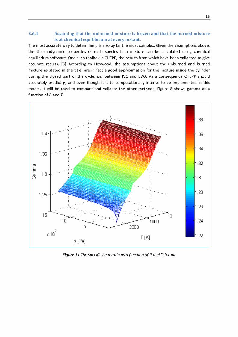
2.6.4 Assuming that the unburned mixture is frozen and that the burned mixture

is at chemical equilibrium at every instant.

The most accurate way to determine is also by far the most complex. Given the assumptions above,

the thermodynamic properties of each species in a mixture can be calculated using chemical

equilibrium software. One such toolbox is CHEPP, the results from which have been validated to give

accurate results. [5] According to Heywood, the assumptions about the unburned and burned

mixture as stated in the title, are in fact a good approximation for the mixture inside the cylinder

during the closed part of the cycle, i.e. between IVC and EVO. As a consequence CHEPP should

accurately predict , and even though it is to computationally intense to be implemented in this

model, it will be used to compare and validate the other methods. Figure 8 shows gamma as a

function of and .

Figure 11 The specific heat ratio as a function of and for air

16

2.6.5 Chosen concept

For this model the method suggested by Klein is used. [3] This approach calls for a linear model in

during the compression. Care must be taken to find the right coefficients for the temperature

interval in question, a table of for air as a function of has been used to find the coefficients. [1]

(13)

In equation (13) and denote the specific heat at constant volume and constant

pressure respectively at , and are constants. To account for EGR, an

interpolation is made between and where the latter is calculated using the

same correlations as during the exhaust stroke. A small correction term to account for internal EGR is

also added. Thus can be written as

(14)

During combustion and the subsequent expansion stroke the polynomial model by Krieger and

Borman is used. For lean and stoichiometric mixtures a single set of polynomials is used.

(15)

It is summarized by equation (14) where

(16)

and

(17)

The gas constant, , is given by:

(18)

The correction terms, and are used to account for dissociation when , while

they are zero for low and moderate temperatures. They are calculated using the formulas described

in [3]. Thus the specific heat ratio can be estimated using the above correlations.

(19)

Where , is obtained by differentiating (15) with respect to T, which results in (19).

(20)

17

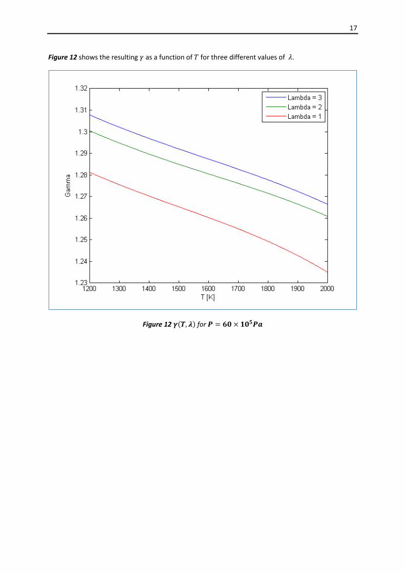
Figure 12 shows the resulting as a function of for three different values of .

Figure 12 for

18

2.7 Fuel Injection To capture all the phenomena that occur in a modern common rail injection system, extensive and

sophisticated hydraulic models are required. However, if certain assumptions are made, the injection

rate can be modeled in a relatively straight forward and simple manner that does not require a lot of

computing time. [1] The pressure upstream of the injector nozzles is assumed to be identical to the

pressure in the fuel rail; any pressure drop over the interior of the fuel injector is neglected.

Furthermore, the flow through the nozzles is assumed to adhere to the following properties:

Quasi steady

Incompressible

One dimensional

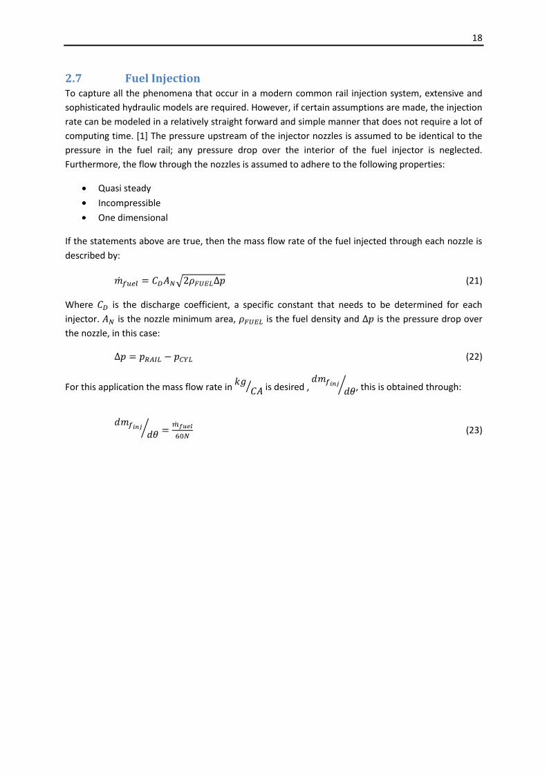
If the statements above are true, then the mass flow rate of the fuel injected through each nozzle is

described by:

(21)

Where is the discharge coefficient, a specific constant that needs to be determined for each

injector. is the nozzle minimum area, is the fuel density and is the pressure drop over

the nozzle, in this case:

(22)

For this application the mass flow rate in is desired , , this is obtained through:

(23)

19

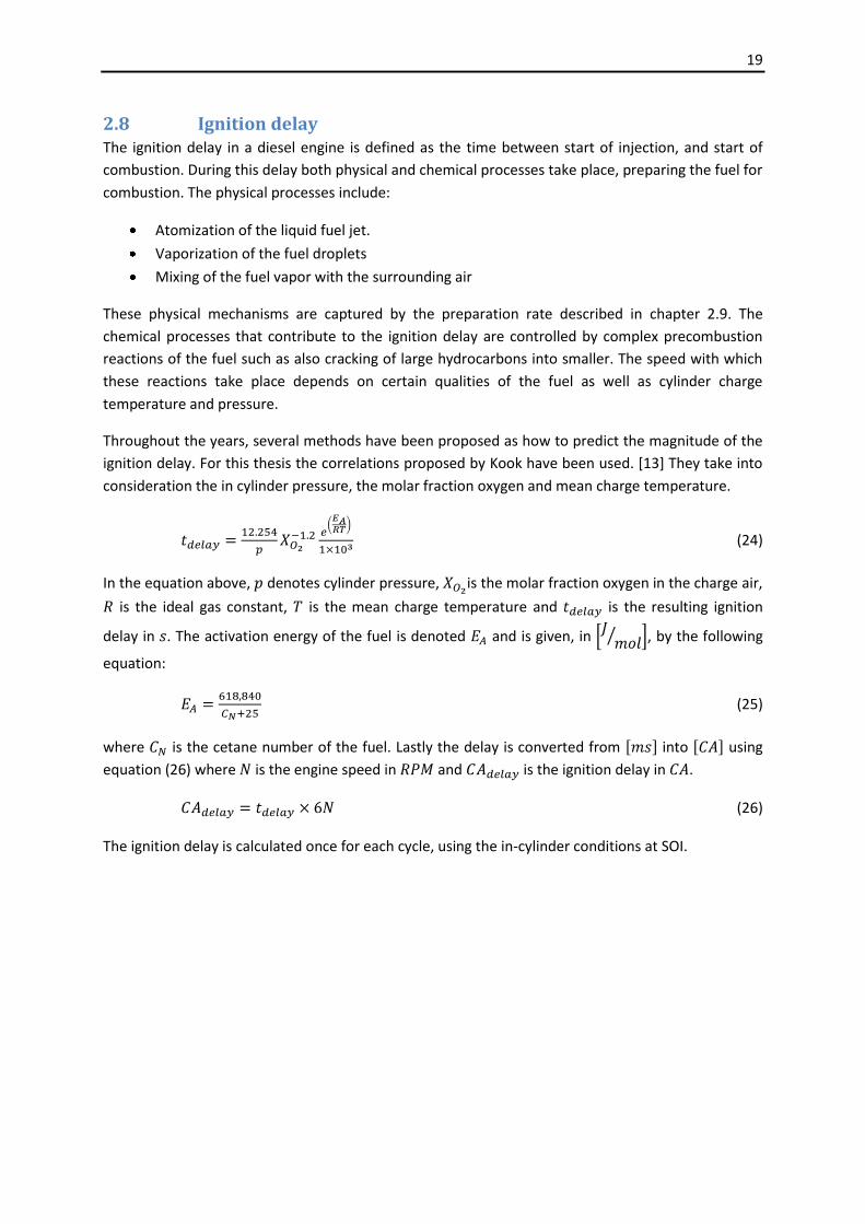
2.8 Ignition delay The ignition delay in a diesel engine is defined as the time between start of injection, and start of

combustion. During this delay both physical and chemical processes take place, preparing the fuel for

combustion. The physical processes include:

Atomization of the liquid fuel jet.

Vaporization of the fuel droplets

Mixing of the fuel vapor with the surrounding air

These physical mechanisms are captured by the preparation rate described in chapter 2.9. The

chemical processes that contribute to the ignition delay are controlled by complex precombustion

reactions of the fuel such as also cracking of large hydrocarbons into smaller. The speed with which

these reactions take place depends on certain qualities of the fuel as well as cylinder charge

temperature and pressure.

Throughout the years, several methods have been proposed as how to predict the magnitude of the

ignition delay. For this thesis the correlations proposed by Kook have been used. [13] They take into

consideration the in cylinder pressure, the molar fraction oxygen and mean charge temperature.

(24)

In the equation above, denotes cylinder pressure, is the molar fraction oxygen in the charge air,

is the ideal gas constant, is the mean charge temperature and is the resulting ignition

delay in . The activation energy of the fuel is denoted and is given, in , by the following

equation:

(25)

where is the cetane number of the fuel. Lastly the delay is converted from into using

equation (26) where is the engine speed in and is the ignition delay in .

(26)

The ignition delay is calculated once for each cycle, using the in-cylinder conditions at SOI.

20

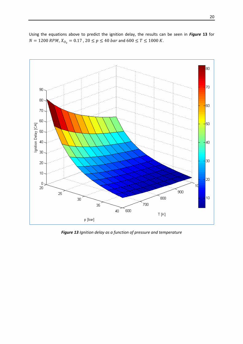
Using the equations above to predict the ignition delay, the results can be seen in Figure 13 for

, , and .

Figure 13 Ignition delay as a function of pressure and temperature

21

2.9 Fuel Evaporation Fuel evaporation and combustion are described using a semi-empirical model proposed by

Whitehouse and Way and subsequently used by other authors. In this approach the details of the

fuel evaporation, atomization and micro mixing with the entrained air are neglected and all of the

intermediate steps are summarized into what is called the preparation rate. The preparation rate in

turn depends on the total amount of injected fuel up until the present time, the partial oxygen

pressure, and the amount of fuel injected but not yet prepared. These are used to form the following

expression for the preparation rate in :

(27)

Where is the cumulative mass of the injected fuel up to the present crank angle, is the

cumulative mass of injected but not yet prepared fuel, is the partial oxygen pressure in and

and are constants. In turn, is given by:

(28)

where is the fuel mass injection rate. Furthermore, is given by:

(29)

22

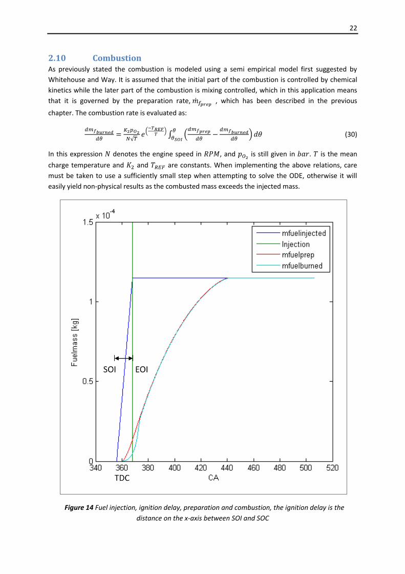
2.10 Combustion As previously stated the combustion is modeled using a semi empirical model first suggested by

Whitehouse and Way. It is assumed that the initial part of the combustion is controlled by chemical

kinetics while the later part of the combustion is mixing controlled, which in this application means

that it is governed by the preparation rate, , which has been described in the previous

chapter. The combustion rate is evaluated as:

(30)

In this expression denotes the engine speed in , and is still given in . is the mean

charge temperature and and are constants. When implementing the above relations, care

must be taken to use a sufficiently small step when attempting to solve the ODE, otherwise it will

easily yield non-physical results as the combusted mass exceeds the injected mass.

Figure 14 Fuel injection, ignition delay, preparation and combustion, the ignition delay is the

distance on the x-axis between SOI and SOC

23

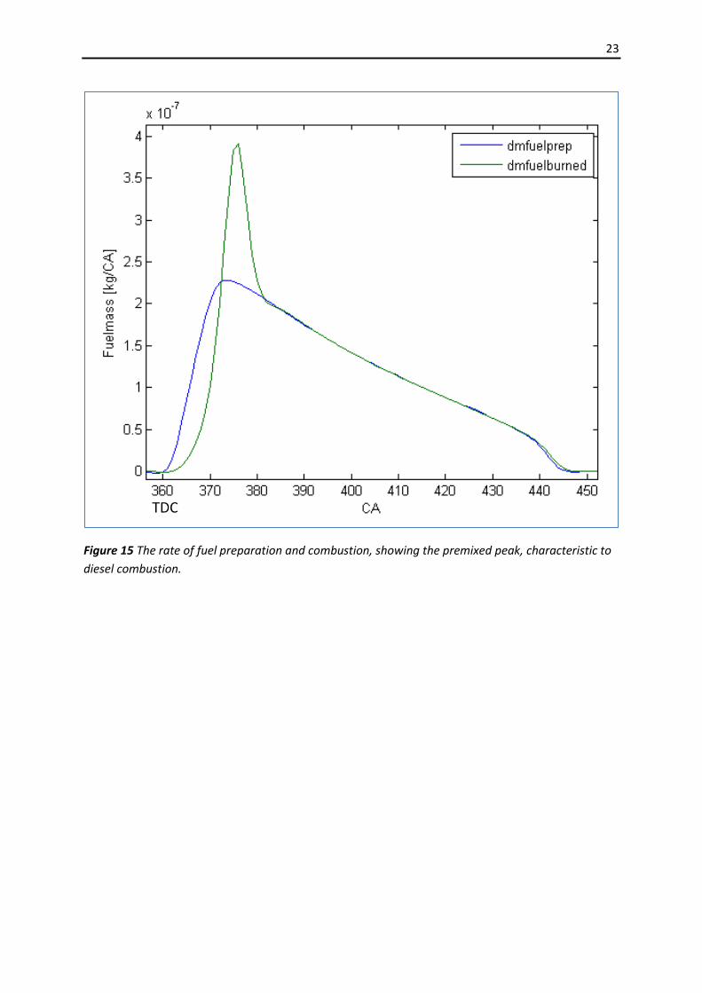
Figure 15 The rate of fuel preparation and combustion, showing the premixed peak, characteristic to

diesel combustion.

24

2.11 Heat Transfer In a combustion engine, the heat transfer from the cylinder charge to the cylinder walls can be

divided into two parts, governed by different mechanisms. There is convective heat transfer, where

heat is transferred through fluids in motion or between a fluid and a solid surface. If the fluid has

motion caused by factors other than gravity, such as the case in the cylinder of a running engine, it is

called forced convection. Along with the forced convection there is also radiative heat transfer,

where the heat transfers through emission and absorption of electromagnetic waves.

To make possible accurate cycle simulations a way of approximating the instantaneous heat flux is

necessary, for this thesis, the model proposed by Woschni is used to predict convective heat transfer,

in addition, the radiation term proposed by Annand is used. [1] Thus the correlation is written:

(31)

where , , and are constants, is the approximate wall temperature, is the Boltzmann

constant and is the average cylinder gas velocity, which in turn is given as:

(32)

and are constants, is the mean piston velocity, is the displaced volume and

describe the conditions in the cylinder at a certain known reference point, such as SOI. Woschni

assumed that the mean gas velocity in the cylinder, an important factor for convection, is

proportional to the mean piston speed. The turbulence caused by combustion, he reasoned, is

proportional to the pressure increase due to the aforementioned combustion, represented by the

term , where is the cylinder pressure and is the corresponding pressure from a

motored cycle. [1]

The mean piston velocity is:

(33)

Where is the engine speed and is the throw radius.

25

3 Validation

3.1 Experimental setup The measurements have been carried out on a single cylinder lab engine available at the Royal

Institute of Technology in Stockholm, Sweden.

Figure 16 Single cylinder lab engine used to validate the model

The engine has a displacement of 2 l and is equipped with a modern high pressure common rail

system and a Scania XPI injector. The piston and piston crown are also from Scania, Euro V standard.

The cylinder head can be replaced with a hydraulic free valve system from Lotus Engineering which

enables variable valve timing and lift, completely independent of the crank shaft.

Auxiliary systems are in place for heating or cooling of intake air, oil, fuel and water. A supercharged

SAAB engine is run in an adjacent room, providing hydraulic pressure for the brake and supplying the

EGR when desired. When evaluating the data, the stoichiometric EGR from the SAAB engine is

translated into the equivalent EGR ratio, had the EGR been generated at the current operating

conditions.

The cylinder pressure is measured using a Kistler pressure transducer mounted in the cylinder head.

The signal is amplified by a Kistler 5011 charge amplifier. A Horiba exhaust gas analyser evaluates the

emissions. The test bed is also equipped with an AVL Smoke Meter, an AVL Opacimeter and a particle

counter.

The operation of the engine, the auxiliary systems and actuators and the data acquisition systems are

controlled by a single PC software, Cell4, which is supported by several PIC-processors.

26

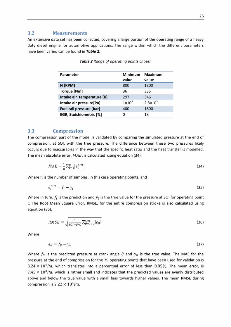
3.2 Measurements An extensive data set has been collected, covering a large portion of the operating range of a heavy

duty diesel engine for automotive applications. The range within which the different parameters

have been varied can be found in Table 2.

Table 2 Range of operating points chosen

3.3 Compression The compression part of the model is validated by comparing the simulated pressure at the end of

compression, at SOI, with the true pressure. The difference between these two pressures likely

occurs due to inaccuracies in the way that the specific heat ratio and the heat transfer is modelled.

The mean absolute error, , is calculated using equation (34).

(34)

Where is the number of samples, in this case operating points, and

(35)

Where in turn, is the prediction and is the true value for the pressure at SOI for operating point

. The Root Mean Square Error, RMSE, for the entire compression stroke is also calculated using

equation (36).

(36)

Where

(37)

Where is the predicted pressure at crank angle and is the true value. The MAE for the

pressure at the end of compression for the 79 operating points that have been used for validation is

, which translates into a percentual error of less than . The mean error, is

, which is rather small and indicates that the predicted values are evenly distributed

above and below the true value with a small bias towards higher values. The mean RMSE during

compression is .

Parameter Minimum value

Maximum value

N [RPM] 800 1800

Torque [Nm] 36 335

Intake air temperature [K] 297 346

Intake air pressure[Pa] 1×105 2.8×105

Fuel rail pressure [bar] 400 1800

EGR, Stoichiometric [%] 0 18

27

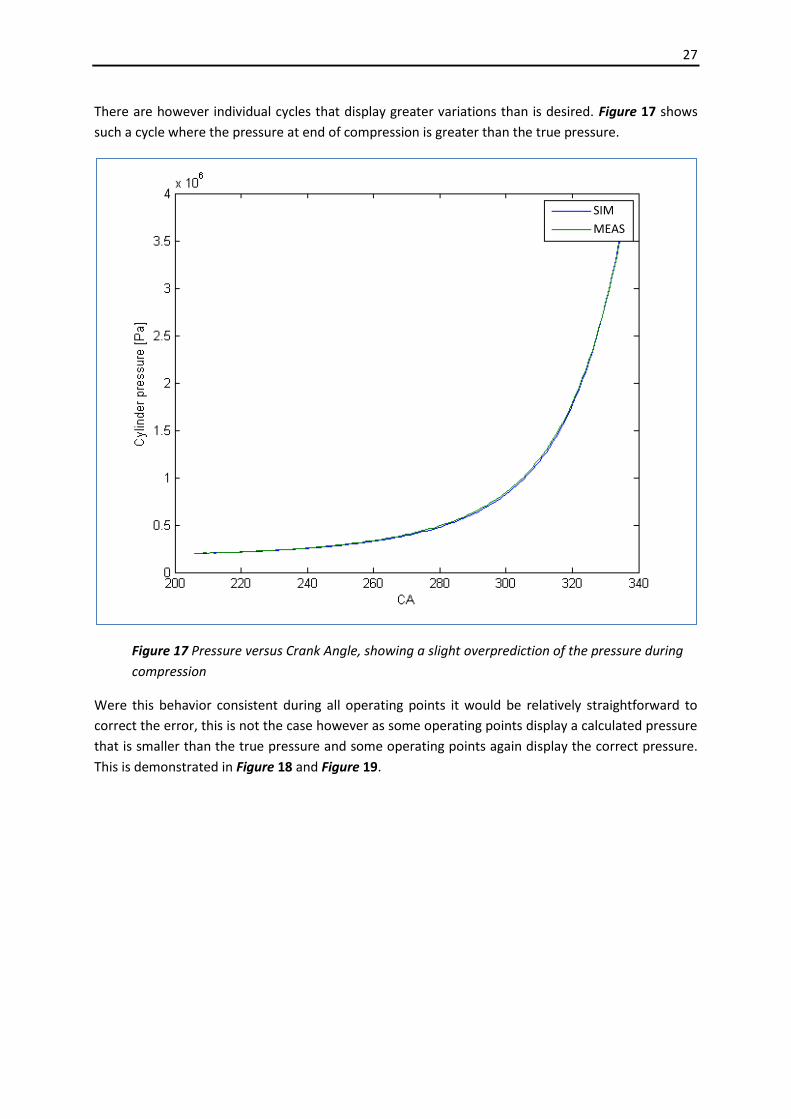
There are however individual cycles that display greater variations than is desired. Figure 17 shows

such a cycle where the pressure at end of compression is greater than the true pressure.

Figure 17 Pressure versus Crank Angle, showing a slight overprediction of the pressure during

compression

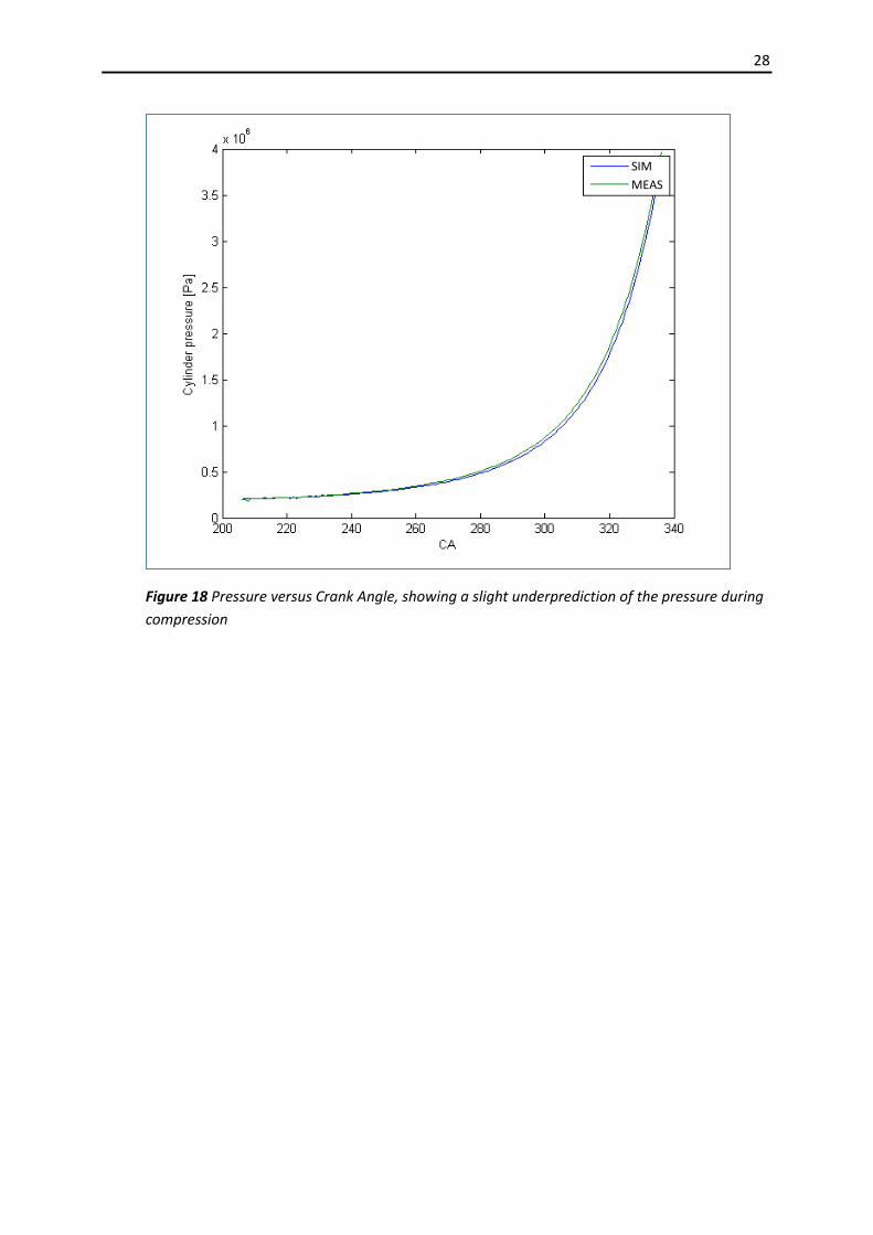
Were this behavior consistent during all operating points it would be relatively straightforward to

correct the error, this is not the case however as some operating points display a calculated pressure

that is smaller than the true pressure and some operating points again display the correct pressure.

This is demonstrated in Figure 18 and Figure 19.

SIM

MEAS

28

Figure 18 Pressure versus Crank Angle, showing a slight underprediction of the pressure during

compression

SIM

MEAS

29

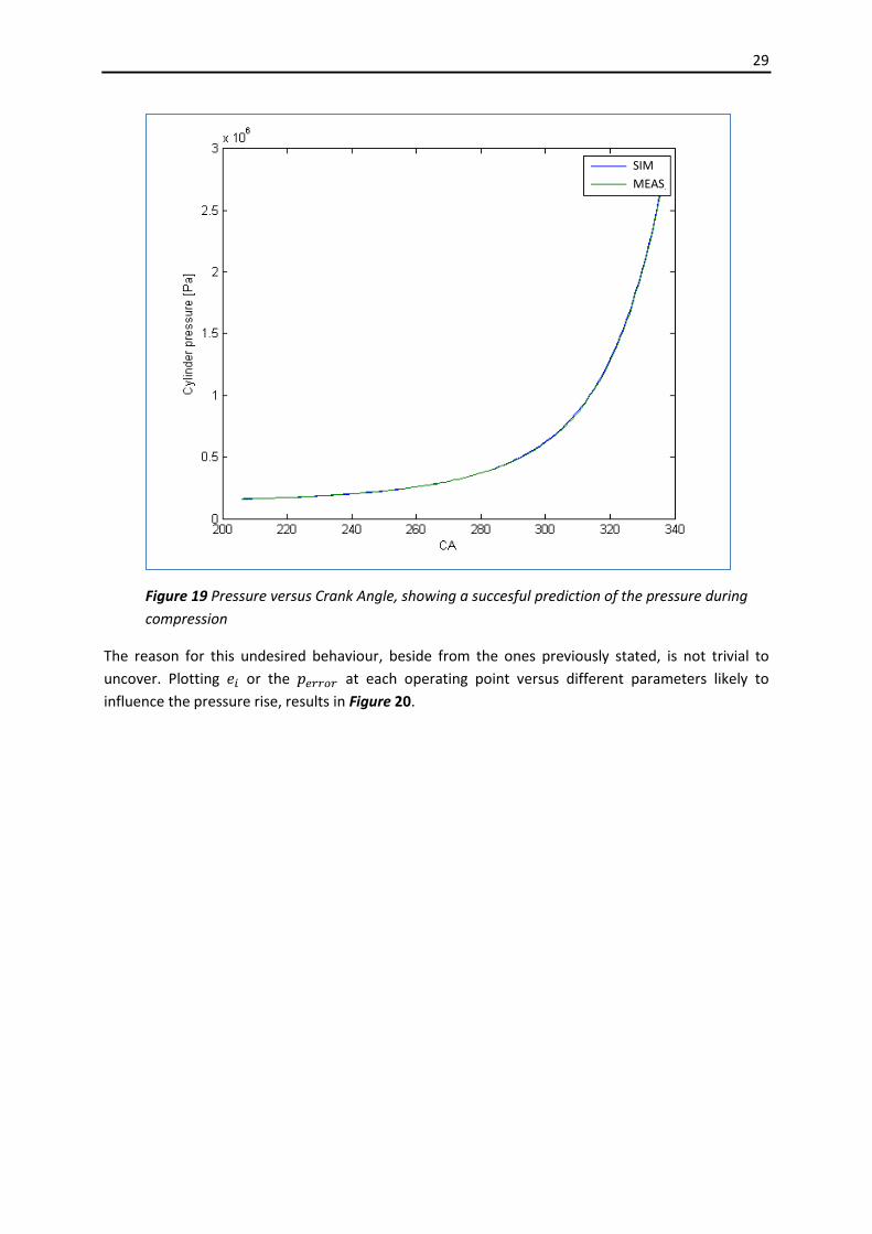
Figure 19 Pressure versus Crank Angle, showing a succesful prediction of the pressure during

compression

The reason for this undesired behaviour, beside from the ones previously stated, is not trivial to

uncover. Plotting or the at each operating point versus different parameters likely to

influence the pressure rise, results in Figure 20.

SIM

MEAS

30

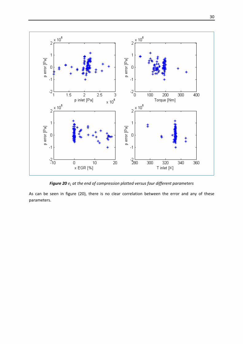
Figure 20 at the end of compression plotted versus four different parameters

As can be seen in figure (20), there is no clear correlation between the error and any of these

parameters.

31

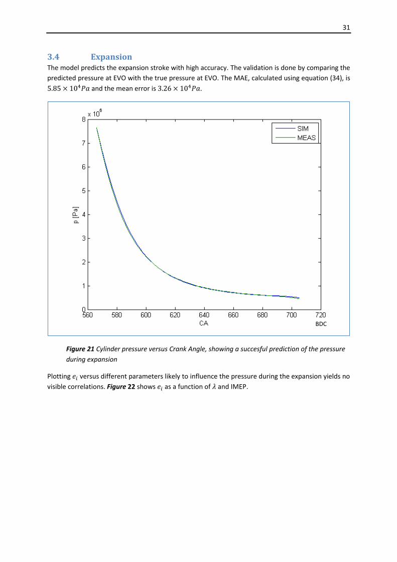
3.4 Expansion The model predicts the expansion stroke with high accuracy. The validation is done by comparing the

predicted pressure at EVO with the true pressure at EVO. The MAE, calculated using equation (34), is

and the mean error is .

Figure 21 Cylinder pressure versus Crank Angle, showing a succesful prediction of the pressure

during expansion

Plotting versus different parameters likely to influence the pressure during the expansion yields no

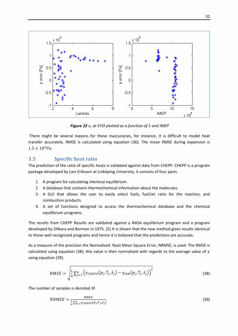
visible correlations. Figure 22 shows as a function of and IMEP.

BDC

32

Figure 22 at EVO plotted as a function of and IMEP

There might be several reasons for these inaccuracies, for instance, it is difficult to model heat

transfer accurately. RMSE is calculated using equation (36). The mean RMSE during expansion is

.

3.5 Specific heat ratio The prediction of the ratio of specific heats is validated against data from CHEPP. CHEPP is a program

package developed by Lars Eriksson at Linköping University, it consists of four parts.

1. A program for calculating chemical equilibrium.

2. A database that contains thermochemical information about the molecules.

3. A GUI that allows the user to easily select fuels, fuel/air ratio for the reaction, and

combustion products.

4. A set of functions designed to access the thermochemical database and the chemical

equilibrium programs.

The results from CHEPP Results are validated against a NASA equilibrium program and a program

developed by Olikara and Borman in 1975. [5] It is shown that the new method gives results identical

to those well recognized programs and hence it is believed that the predictions are accurate.

As a measure of the precision the Normalized Root Mean Square Error, NRMSE, is used. The RMSE is

calculated using equation (38); this value is then normalized with regards to the average value of

using equation (39).

(38)

The number of samples is denoted .

(39)

33

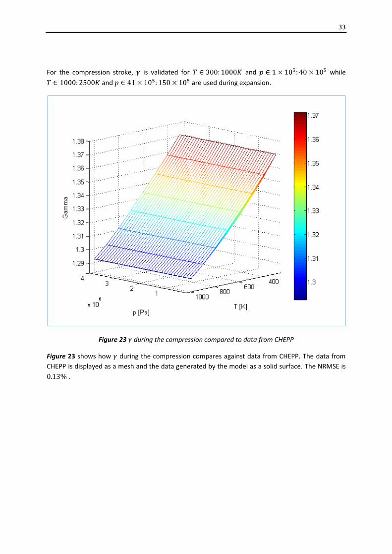
For the compression stroke, is validated for and while

and are used during expansion.

Figure 23 during the compression compared to data from CHEPP

Figure 23 shows how during the compression compares against data from CHEPP. The data from

CHEPP is displayed as a mesh and the data generated by the model as a solid surface. The NRMSE is

.

34

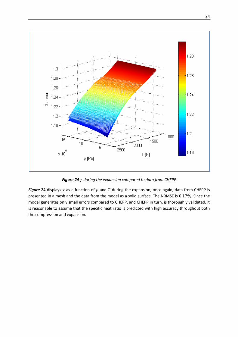
Figure 24 during the expansion compared to data from CHEPP

Figure 24 displays as a function of and during the expansion, once again, data from CHEPP is

presented in a mesh and the data from the model as a solid surface. The NRMSE is . Since the

model generates only small errors compared to CHEPP, and CHEPP in turn, is thoroughly validated, it

is reasonable to assume that the specific heat ratio is predicted with high accuracy throughout both

the compression and expansion.

35

3.6 Fuel Injection The injection of fuel is described using equations (21) to (23). The parameter , the discharge

coefficient, needs to be tuned for each specific fuel injector, it also varies with the amount of fuel

injected. This is one source of inaccuracy; however it is not the most severe. The injection delay,

, which is the time that passes between the ECU injection command and the effective

injector opening. This delay was not constant for the engine setup used, instead it varied in a way

that was not easy to predict and outside the scope of this essay. A delay of , which

corresponds to roughly 3-6 CA at 2000 RPM, affects the combustion phasing and the location and

magnitude of .

When using short injection durations, for instance when using pilot or post injections or when

running at low loads, the duration of the injection is in the same order of magnitude as .In

these cases the uncertainty in causes the predicted amount of injected fuel to deviate from

the true value by as much as a factor of two or more.

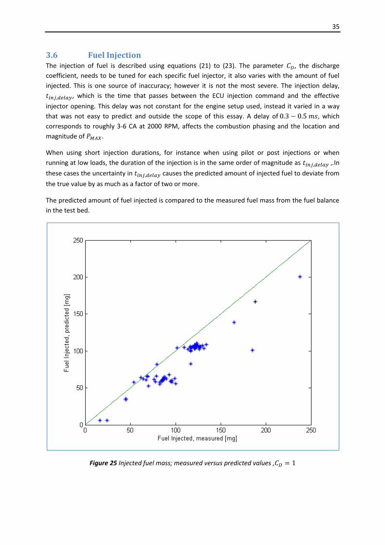
The predicted amount of fuel injected is compared to the measured fuel mass from the fuel balance

in the test bed.

Figure 25 Injected fuel mass; measured versus predicted values ,

36

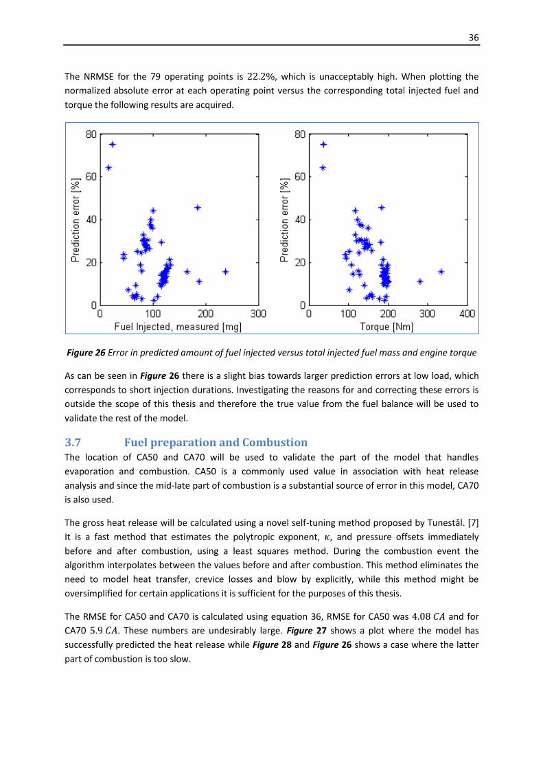
The NRMSE for the 79 operating points is , which is unacceptably high. When plotting the

normalized absolute error at each operating point versus the corresponding total injected fuel and

torque the following results are acquired.

Figure 26 Error in predicted amount of fuel injected versus total injected fuel mass and engine torque

As can be seen in Figure 26 there is a slight bias towards larger prediction errors at low load, which

corresponds to short injection durations. Investigating the reasons for and correcting these errors is

outside the scope of this thesis and therefore the true value from the fuel balance will be used to

validate the rest of the model.

3.7 Fuel preparation and Combustion The location of CA50 and CA70 will be used to validate the part of the model that handles

evaporation and combustion. CA50 is a commonly used value in association with heat release

analysis and since the mid-late part of combustion is a substantial source of error in this model, CA70

is also used.

The gross heat release will be calculated using a novel self-tuning method proposed by Tunestål. [7]

It is a fast method that estimates the polytropic exponent, , and pressure offsets immediately

before and after combustion, using a least squares method. During the combustion event the

algorithm interpolates between the values before and after combustion. This method eliminates the

need to model heat transfer, crevice losses and blow by explicitly, while this method might be

oversimplified for certain applications it is sufficient for the purposes of this thesis.

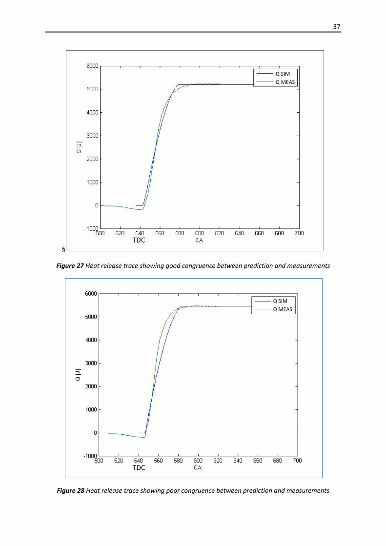
The RMSE for CA50 and CA70 is calculated using equation 36, RMSE for CA50 was and for

CA70 . These numbers are undesirably large. Figure 27 shows a plot where the model has

successfully predicted the heat release while Figure 28 and Figure 26 shows a case where the latter

part of combustion is too slow.

37

§

Figure 27 Heat release trace showing good congruence between prediction and measurements

Figure 28 Heat release trace showing poor congruence between prediction and measurements

Q SIM

Q MEAS

Q SIM

Q MEAS

38

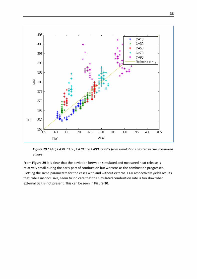
Figure 29 CA10, CA30, CA50, CA70 and CA90, results from simulations plotted versus measured

values

From Figure 29 it is clear that the deviation between simulated and measured heat release is

relatively small during the early part of combustion but worsens as the combustion progresses.

Plotting the same parameters for the cases with and without external EGR respectively yields results

that, while inconclusive, seem to indicate that the simulated combustion rate is too slow when

external EGR is not present. This can be seen in Figure 30.

MEAS

39

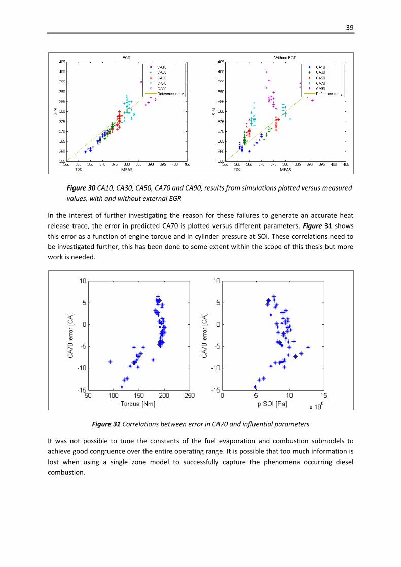
Figure 30 CA10, CA30, CA50, CA70 and CA90, results from simulations plotted versus measured

values, with and without external EGR

In the interest of further investigating the reason for these failures to generate an accurate heat

release trace, the error in predicted CA70 is plotted versus different parameters. Figure 31 shows

this error as a function of engine torque and in cylinder pressure at SOI. These correlations need to

be investigated further, this has been done to some extent within the scope of this thesis but more

work is needed.

Figure 31 Correlations between error in CA70 and influential parameters

It was not possible to tune the constants of the fuel evaporation and combustion submodels to

achieve good congruence over the entire operating range. It is possible that too much information is

lost when using a single zone model to successfully capture the phenomena occurring diesel

combustion.

MEAS MEAS TDC TDC

40

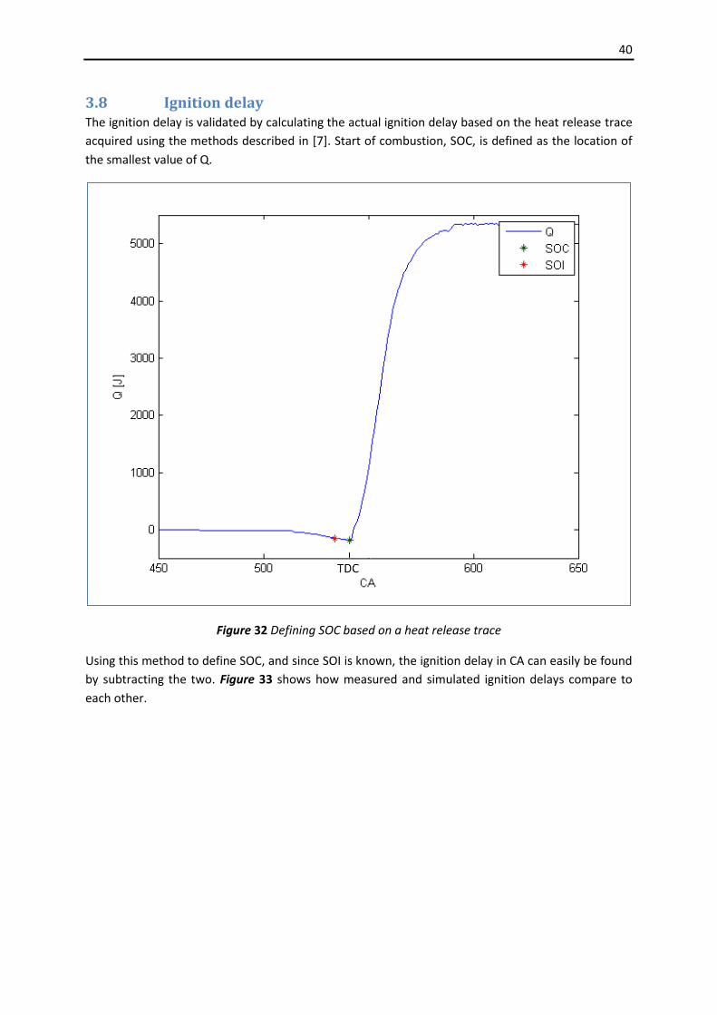
3.8 Ignition delay The ignition delay is validated by calculating the actual ignition delay based on the heat release trace

acquired using the methods described in [7]. Start of combustion, SOC, is defined as the location of

the smallest value of Q.

Figure 32 Defining SOC based on a heat release trace

Using this method to define SOC, and since SOI is known, the ignition delay in CA can easily be found

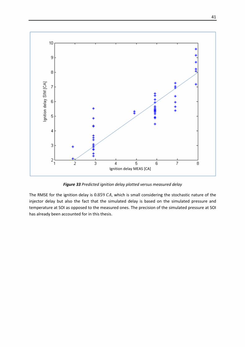
by subtracting the two. Figure 33 shows how measured and simulated ignition delays compare to

each other.

41

Figure 33 Predicted ignition delay plotted versus measured delay

The RMSE for the ignition delay is , which is small considering the stochastic nature of the

injector delay but also the fact that the simulated delay is based on the simulated pressure and

temperature at SOI as opposed to the measured ones. The precision of the simulated pressure at SOI

has already been accounted for in this thesis.

Ignition delay MEAS [CA]

42

3.9 Heat Transfer The method used to predict heat flux, as proposed by Woschni, relies in no small part on careful

tuning of different parameters corresponding to swirl number and other attributes that are both

specific to a certain engine and to a certain operating point.

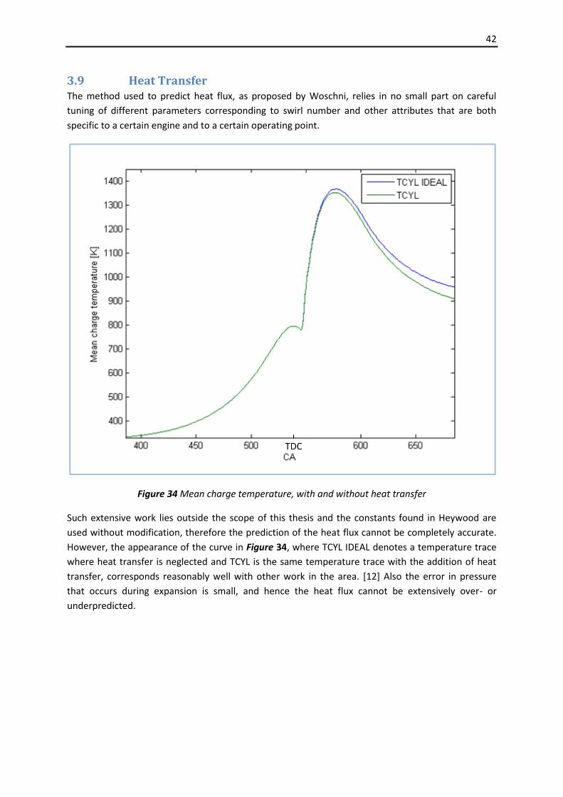
Figure 34 Mean charge temperature, with and without heat transfer

Such extensive work lies outside the scope of this thesis and the constants found in Heywood are

used without modification, therefore the prediction of the heat flux cannot be completely accurate.

However, the appearance of the curve in Figure 34, where TCYL IDEAL denotes a temperature trace

where heat transfer is neglected and TCYL is the same temperature trace with the addition of heat

transfer, corresponds reasonably well with other work in the area. [12] Also the error in pressure

that occurs during expansion is small, and hence the heat flux cannot be extensively over- or

underpredicted.

43

3.10 Closed Cycle For validation of the closed cycle, Indicated Mean Effective Pressure, IMEP, is used to compare the

simulated pressure trace with the measure one. IMEP only takes the closed part of the cycle into

consideration, and compares to Net Mean Effective Pressure, NMEP, according to equation (40)

where PMEP stands for Pumping Mean Effective Pressure.

(40)

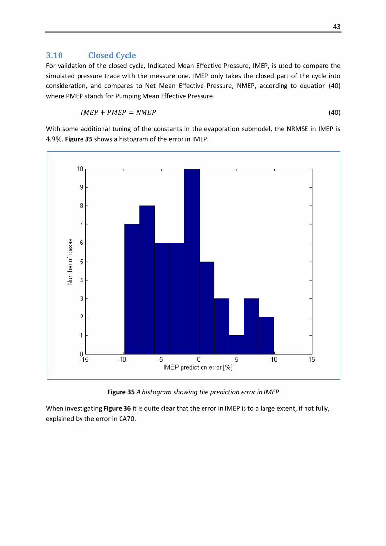
With some additional tuning of the constants in the evaporation submodel, the NRMSE in IMEP is

. Figure 35 shows a histogram of the error in IMEP.

Figure 35 A histogram showing the prediction error in IMEP

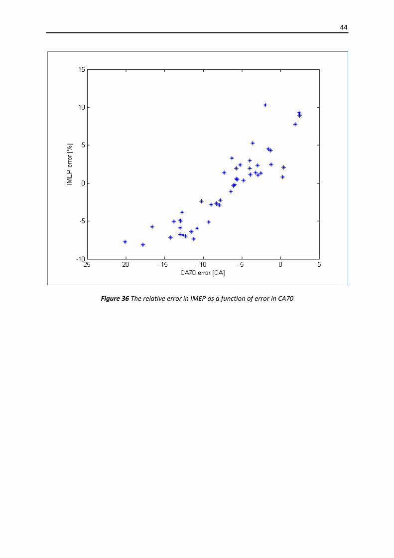
When investigating Figure 36 it is quite clear that the error in IMEP is to a large extent, if not fully,

explained by the error in CA70.

44

Figure 36 The relative error in IMEP as a function of error in CA70

45

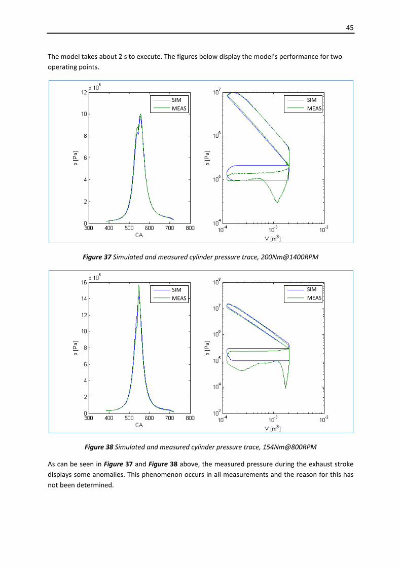
The model takes about 2 s to execute. The figures below display the model’s performance for two

operating points.

Figure 37 Simulated and measured cylinder pressure trace, 200Nm@1400RPM

Figure 38 Simulated and measured cylinder pressure trace, 154Nm@800RPM

As can be seen in Figure 37 and Figure 38 above, the measured pressure during the exhaust stroke

displays some anomalies. This phenomenon occurs in all measurements and the reason for this has

not been determined.

SIM

MEAS

SIM

MEAS

SIM

MEAS

SIM

MEAS

46

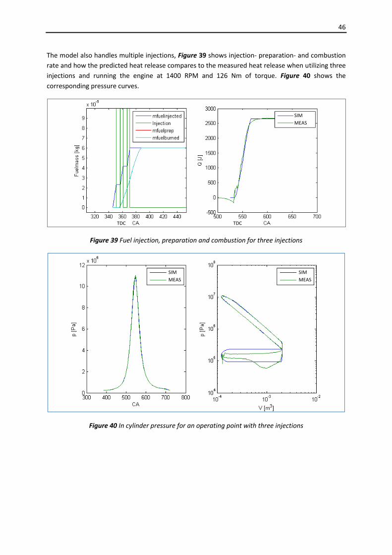
The model also handles multiple injections, Figure 39 shows injection- preparation- and combustion

rate and how the predicted heat release compares to the measured heat release when utilizing three

injections and running the engine at 1400 RPM and 126 Nm of torque. Figure 40 shows the

corresponding pressure curves.

Figure 39 Fuel injection, preparation and combustion for three injections

Figure 40 In cylinder pressure for an operating point with three injections

SIM

MEAS

SIM

MEAS

SIM

MEAS

TDC TDC

47

4 Conclusions A single zone model is developed that predicts the in cylinder pressure during a full cycle for a direct

injected diesel engine. It handles multiple injections and is intended for torque estimation when

calculation speed is of importance. The devised model captures the behavior during compression and

expansion well, the ignition delay and the thermochemical properties of the cylinder charge are also

approximated with satisfactory precision.

During fuel injection and the subsequent combustion, there are complex mechanisms that are not

fully captured by this model and hence require additional attention.

The model executes in about 2 seconds, which corresponds to ten times real time speed at 600 RPM.

It is likely that the execution time can be greatly improved by optimizing the code and removing

unnecessary entries.

The precision of the model is validated against 51 operating points with regards to IMEP, CA50 and

CA70. The RMSE is for CA50 and for CA70. NRMSE for IMEP is .

4.1 Future work When evaluating the model it is clear that certain parts need more work while others provide

satisfactory precision.

The fuel injection introduces the largest error, a prediction error of easily overshadows the

errors generated by all the other submodels and hence it was omitted from the validation. This

needs to be addressed. It is possible that some of the difficulties occur due to hydraulic phenomena

in the fuel rail such as standing waves. Since this is a highly specialized lab engine using a non

standard fuel rail there is a possibility that the injection system has certain attributes unique to this

setup. The injector delay also needs to be investigated further.

To improve the evaporation and combustion modeling, which account for most of the error in IMEP.

the introduction of additional zones in the model should be investigated. After all the conditions in

the combustion chamber of a firing diesel engine are quite heterogeneous and it is possible that the

model is oversimplified and that additional information is required to improve the precision.

48

5 References:

1. J.B.Heywood: Internal Combustion Engine Fundamentals, MCGraw-Hill, Singapore, 1988

2. Dec J. E.: A conceptual model of DI diesel combustion based on laser-sheet imaging, SAE

Technical Paper no. 970873. 1997.

3. M. Klein: A Specific Heat Ratio Model and Compression Ratio Estimation. Licentiate thesis,

Linköping University, 2004.

4. J. Karlsson F. Königsson: Analytical cylinder pressure model for rapid simulations, Technical

report, Department of Internal Combustion Engines, Royal Institute of Technology, 2009

5. L. Eriksson: CHEPP~A chemical equilibrium program package for Matlab, SAE Technical Paper

no. 2004-01-1460. 2004

6. L. Eriksson and I. Andersson: An Analytic Model for Cylinder Pressure in a Four Stroke SI

Engine. SAE Technical Paper no. 2002-01-0371, 2002

7. P. Tunestål: Self-tuning gross heat release computation for internal combustion engines,

Control Engineering Practice, 518-524, 2009

8. OKQ8 Diesel B5 – Miljöklass 1, retrieved January 31, 2010 from OK-Q8 AB, OK-Q8 website:

http://www.okq8.se/servlet/ContentViewerServlet?contentUrl=cycube://internal/document

/105353&nodeId=com.cycube.navigation.node.NodeId@100910

9. Fuel Oils: Chemical and Physical Information, retrieved January 31, 2010 from Agency for

Toxic Substances & Disease Registry, ATSDR website:

http://www.atsdr.cdc.gov/toxprofiles/tp75-c3.pdf

10. Today’s Improved Diesel Engine Technology, retrieved January 31, 2010 from Greencar.com.

Greencar.com website: http://www.greencar.com/articles/todays-improved-diesel-engine-

technology.php

11. Understanding Today’s Diesel, retrieved January 31, 2010 from Banks Power inc., Banks

Power website: http://www.bankspower.com/techarticles/show/26-Understanding-Todays-

Diesel

12. Various authors: Simulation and analysis of combustion and heat transfer in low-heat-

rejection diesel engine using two-zone combustion model and different heat transfer model,

SAE Technical Paper no. 2003-01-1067. 2003

13. S. Kook C. Bae P.C. Miles D. Choi L.M. Pickett: The Influence of Charge Dilution and Injection

Timing on Low-Temperature Diesel Combustion and Emissions, SAE Technical Paper no. 2005-

01-3837. 2005

14. 3D-CFD Simulation Hydrogen High-Pressure-Injector, retrieved February 10, 2010 from

Worldcarfans.com, Worldcarfans.comwebsite: http://www.worldcarfans.com/

109031317856/bmw-hydrogen-engine-project-improves-efficiency--on-par-with-diesel-

engines/lowphotos#4

49

6 Abbreviations

TDC Top Dead Center

BDC Bottom Dead Center

CI Compression Ignited

CN Cetane Number

NOX Nitrous Oxides

SCR Selective Catalytic Reduction

EGR Exhaust Gas Recirculation

CFD Computational Fluid Dynamics

ODE Ordinary Differential Equations

IVO Crank angle of Intake Valve Opening

IVC Crank angle of Intake Valve Closing

EVO Crank angle of Exhaust Valve Opening

EVC Crank angle of Exhaust Valve Closing

SOI Crank angle of Start Of Injection

SOC Crank angle of Start Of Combustion

ECU Engine Control Unit

CA Crank Angles

RPM Revolutions Per Minute

MAE Mean Absolute Error

RMSE Root Mean Square Error

NRMSE Normalized Root Mean Square Error

IMEP Indicated Mean Effective Pressure, high pressure cycle

PMEP Pumping Mean Effective Pressure

NMEP Net Mean Effective Pressure, indicated

CA50 Crank Angle for 50% heat release

CA70 Crank Angle for 70% heat release

50

Appendix A: Constants

Constant Value Used