
A chaotic model for the epidemic of Ebola virus disease in West Africa (2013–2016)Sylvain Mangiarotti, Marisa Peyre, and Mireille Huc Citation: Chaos 26, 113112 (2016); doi: 10.1063/1.4967730 View online: http://dx.doi.org/10.1063/1.4967730 View Table of Contents: http://scitation.aip.org/content/aip/journal/chaos/26/11?ver=pdfcov Published by the AIP Publishing Articles you may be interested in Computational model of a vector-mediated epidemic Am. J. Phys. 83, 468 (2015); 10.1119/1.4917164 Epidemic spreading in time-varying community networks Chaos 24, 023116 (2014); 10.1063/1.4876436 Evolution of N-species Kimura/voter models towards criticality, a surrogate for general models of accidentalpathogens AIP Conf. Proc. 1479, 1331 (2012); 10.1063/1.4756401 The impact of awareness on epidemic spreading in networks Chaos 22, 013101 (2012); 10.1063/1.3673573 Generalized entropies of chaotic maps and flows: A unified approach Chaos 7, 694 (1997); 10.1063/1.166267
Reuse of AIP Publishing content is subject to the terms at: https://publishing.aip.org/authors/rights-and-permissions. Downloaded to IP: 193.51.119.103 On: Thu, 08 Dec
2016 14:23:21
A chaotic model for the epidemic of Ebola virus disease in West Africa(2013–2016)
Sylvain Mangiarotti,1 Marisa Peyre,2 and Mireille Huc1
1Centre d’ �Etudes Spatiales de la Biosphere, CNRS-UPS-CNES-IRD, Observatoire Midi-Pyr�en�ees,18 Avenue �Edouard Belin, 31401 Toulouse, France2UPR AGIRs, Bureau 208, Batiment E TA C22/E, Centre de Coop�eration Internationale en RechercheAgronomique pour le D�eveloppement (CIRAD), Campus International de Baillarguet,Montpellier Cedex 5 34398, France
(Received 9 August 2016; accepted 28 October 2016; published online 16 November 2016)
An epidemic of Ebola Virus Disease (EVD) broke out in Guinea in December 2013. It was only
identified in March 2014 while it had already spread out in Liberia and Sierra Leone. The spill over
of the disease became uncontrollable and the epidemic could not be stopped before 2016. The time
evolution of this epidemic is revisited here with the global modeling technique which was designed
to obtain the deterministic models from single time series. A generalized formulation of this
technique for multivariate time series is introduced. It is applied to the epidemic of EVD in West
Africa focusing on the period between March 2014 and January 2015, that is, before any detected
signs of weakening. Data gathered by the World Health Organization, based on the official
publications of the Ministries of Health of the three main countries involved in this epidemic, are
considered in our analysis. Two observed time series are used: the daily numbers of infections and
deaths. A four-dimensional model producing a very complex dynamical behavior is obtained. The
model is tested in order to investigate its skills and drawbacks. Our global analysis clearly helps to
distinguish three main stages during the epidemic. A characterization of the obtained attractor is
also performed. In particular, the topology of the chaotic attractor is analyzed and a skeleton is
obtained for its structure. Published by AIP Publishing. [http://dx.doi.org/10.1063/1.4967730]
Mathematical models can offer useful insight to analyze
and forecast the evolution of epidemics in expansion. A
generalized version of the global modeling technique is
introduced here and applied to the epidemic of Ebola
Virus Disease (EVD) that broke out in West Africa in
December 2013. The analysis clearly permits to distin-
guish three main stages during the outbreak: (i) the ear-
lier development of the epidemic in remote regions, (ii)
the uncontrolled period of rapid propagation of the dis-
ease in urban regions, and (iii) its long slowdown until it
could end. The obtained model shows that the epidemic is
governed by a low-dimensional chaotic dynamics. The
resulting four-dimensional chaotic attractor is analyzed
in terms of the dynamical, geometrical, and structural
properties. To characterize the topology of this attractor,
a skeleton is proposed for its four-dimensional chaos.
I. INTRODUCTION
When an epidemic is in expansion, it is important to
have approaches that can be applied to scarce data sets. This
is especially true for emerging and reemerging diseases, for
which causes and transfer processes are often poorly known
and understood. It is also the case for epidemics of well
understood diseases for which dynamics may vary from one
focus to another, and more especially when the disease is
characterized by high levels of lethality. Ebola virus and
Marburg diseases are among these.
Most of the models developed to simulate infectious dis-
eases are issued from the pioneering work of Kermack and
McKendrick1 initially designed to model plague epidemics.
These models divide the population in compartments that
generally distinguish Susceptible, Infected, Recovered and
possibly also Exposed and other classes of a given popula-
tion. Compartment models can be applied to one or several
species and thus to epidemics, epizootics, and coupled epi-
demics and epizootics. Such models have proven to be useful
to better understand the epidemics, and can be used today to
model the Ebola virus epidemic.2–5 Nevertheless, modeling
epidemics in general, and Ebola epidemics in particular,
remains a quite difficult problem, in particular, because of
the large variability of dynamics that can be observed from
one outbreak to another. Such diversity appears flagrant for
Ebola virus epidemics when comparing the West Africa
Ebola outbreak of 20146 (for which total number of reported
cases and deaths are extremely high, 28 652 and 11 325,
respectively) to any of the outbreaks that occurred previously
or concurrently in central Africa7 (�425 infections and
�280 deaths, laboratory confirmed cases only).
Such monitoring is especially difficult for emerging dis-
eases for which it is sometimes required to consider simulta-
neously unprecedented humanitarian crisis together with
the fundamental and applied scientific challenges in order to
identify the various reservoirs contributing to the propaga-
tion of the disease and to understand the processes at
work, with the aim to slow down and if possible to stop the
epidemic. The large number of factors involved in a disease
1054-1500/2016/26(11)/113112/15/$30.00 Published by AIP Publishing.26, 113112-1
CHAOS 26, 113112 (2016)
Reuse of AIP Publishing content is subject to the terms at: https://publishing.aip.org/authors/rights-and-permissions. Downloaded to IP: 193.51.119.103 On: Thu, 08 Dec
2016 14:23:21
generally make the task particularly complex, since it
includes a wide diversity of intertwined problems of diag-
nostics, management, biology, ecology, society, economic,
environment, etc. Such problems are all present in an epi-
demic such as Ebola6,8 and especially difficult to take into
account in a modeling approach.
Since often facing a strong non-stationarity of the
dynamical behavior—in space and in time—it would be use-
ful to develop pragmatic approaches for such contexts.
Indeed, it is necessary to explore the alternative methods to
forecast the time evolution of the disease that, for instance,
would help for the estimation of the urgent needs in a more
pragmatic way.
This may be done by directly fitting compartment mod-
els to the data in order to adapt the models to the current con-
text. Indeed, processes modeling can be very useful to better
understand the dynamics of a disease. An ad hoc calibration
of such models may provide useful simulations but it
requires its algebraic formulation to be well adapted to the
dynamical context. Unfortunately, a proper calibration may
require a complete set of local information to parameterize
the model appropriately. In many cases, local information is
missing, and it is necessary to reuse information from other
sites of study and/or previous outbreaks, assuming stationary
conditions in space and time. Such assumption can be haz-
ardous since a information can exhibit an important variabil-
ity in space and time.9 Note that model parameters can
also depend on the aggregation scale10 and thus on the model
spatial representativity. This problem can be met when trans-
porting the model from one outbreak to another.
Moreover, the variations of the algebraic structure
required to model the epidemics can be very different, not
only from one type of disease to another, but also between
several focuses of the same disease. This hypothesis of ergo-
dicity is often very partially satisfied only, and thus hard to
justify. It is especially the case when considering emergent
diseases such as Ebola for which important factors remain
poorly known. In the case of the West Africa Ebola epi-
demic, heterogeneous behaviors could be observed both in
space and time.11 It is quite important to take this difficulty
into account when attempting to model an epidemic in
expansion, especially in a context of scarce data.
The global modeling technique may be a useful and
complementary technique to explore epidemics in such con-
ditions. This technique is based on the theory of nonlinear
dynamical systems that allows a deterministic and strongly
nonlinear point of view fully adapted to analyze the dynam-
ics presenting limited horizons of predictability.
Several models were already obtained from the environ-
mental data based on this technique.12,13 Note that a model of
difference equations could also be obtained for the whooping
cough in London for the period from 1967 to 1990.14
Recently, the approach was applied to a multivariate set of
variables to model the epidemic of plague that occurred in
Bombay at the end of the 19th century.15 In this latter work,
it was shown that it was possible to identify the couplings of
the epidemic of plague with the epizootics of the two main
species of rats.
The objective of the present work is to investigate the
capacity of the global modeling technique to model an epi-
demic of EVD based on a restrictive number of observables,
during the very strong propagation of the disease. The West
Africa epidemic (2013–2016) is considered in this study.
Although the whole period for which data are available is
considered in the analysis, the modeling part is focused on
the period between March 2014 and January 2015, that is,
before any clear breakdown of the epidemic.
Data used in the study and their epidemiological context
are presented in Section II. The global modeling technique is
introduced in Section III. To make it applicable to a couple
of observables, a generalized formulation of the approach is
introduced. Results are presented in Section IV. Discussions
and conclusions are given in Section V.
II. DATA AND CONTEXT
A. General background
EVD is due to an etiological agent of the family of
Filoviridae. It is one of the most serious viral disease cur-
rently known, for which no prophylactic or therapeutic strate-
gies were found. Five species of the Ebola virus are identified
among which Ebola-Zaire strain has the highest level of
lethality, with a rate close to 70%.9
Fruit bats are considered to be the most likely carriers
of the Ebola virus in the wild.16 Three main species of fruit
bats (Hypsignathus monstrosus, Epomops franqueti, and
Myonycteris torquata) have been identified as potential car-
riers, their geographic distribution covers a large area from
Central to West Africa.16 Interestingly, the potential spread of
the EVD had already been estimated based on the ecological
niche modeling in earlier works.17 Although outbreaks remain
quite rare, it is estimated that 22 � 106 of people live in areas
at risk,18 that makes the transmission of Ebola virus from ani-
mal to man possible. Alteration of the biosystems by land-use
change and deforestation has been intensive in this region,
where mosaics of forest and agriculture are now dominating
the countryside.19 This evolution may have increased the prob-
ability of contact between chiroptera and human.
Transfer of the Ebola virus from animals to humans and
between humans can typically occur through contact with
bodily fluids of infected animals and humans. This transfer
may occur during the butchering of bats,20 when consuming
infected bushmeat, when caring for patients21 or when pre-
paring the deceased for burial.5,21,22 The detection of the
disease is made difficult by the fact that most of the symp-
toms of the disease are not specific, and thus difficult to
distinguish from other diseases such as yellow fever and
malaria, also endemic to the region.8
B. Comparative contexts
It was established that the epidemic of EVD that has
swept West Africa from 2013 to 2016 had no link with the
previous epidemics.23 Since the strain of the virus was iden-
tified as Zaire ebolavirus (one of the strains responsible for
several of the previous outbreaks in Central Africa), a similar
behavior could have been expected. It was definitively not
113112-2 Mangiarotti, Peyre, and Huc Chaos 26, 113112 (2016)
Reuse of AIP Publishing content is subject to the terms at: https://publishing.aip.org/authors/rights-and-permissions. Downloaded to IP: 193.51.119.103 On: Thu, 08 Dec
2016 14:23:21
the case and several important elements were evoked to
explain such a strong differentiation. One important reason
may probably be that most of the previous outbreaks
occurred in remote forested areas that are places of low pop-
ulation density with slow connections by road, river, and air,
thus limiting human contacts. Another quite probable reason
may be that an important experience of EVD epidemics has
been acquired in Central Africa.23 This was clearly not the
case in West Africa where health services were found
sharply unprepared,11 due to both the devastating effect of
civil wars in Liberia and Sierra Leone and the very difficult
economic situation in the three involved countries which are
among the poorest countries in the world.24 These elements
have probably played an important role in the present con-
text, although other factors can also have contributed to this
differentiation.
C. Data source and preprocessing
One important objective of the present work is to test
the efficiency of the global modeling technique to obtain a
model based on scarce information (two observables only).
Two time series are used: the number of people infected by
the Ebola virus and the number of resulting deaths. Data are
from the World Health Organization and were downloaded
from the Centers for Disease Control and Prevention.25
These data are reported as cumulative numbers starting from
the beginning of the epidemic and have an irregular sampling
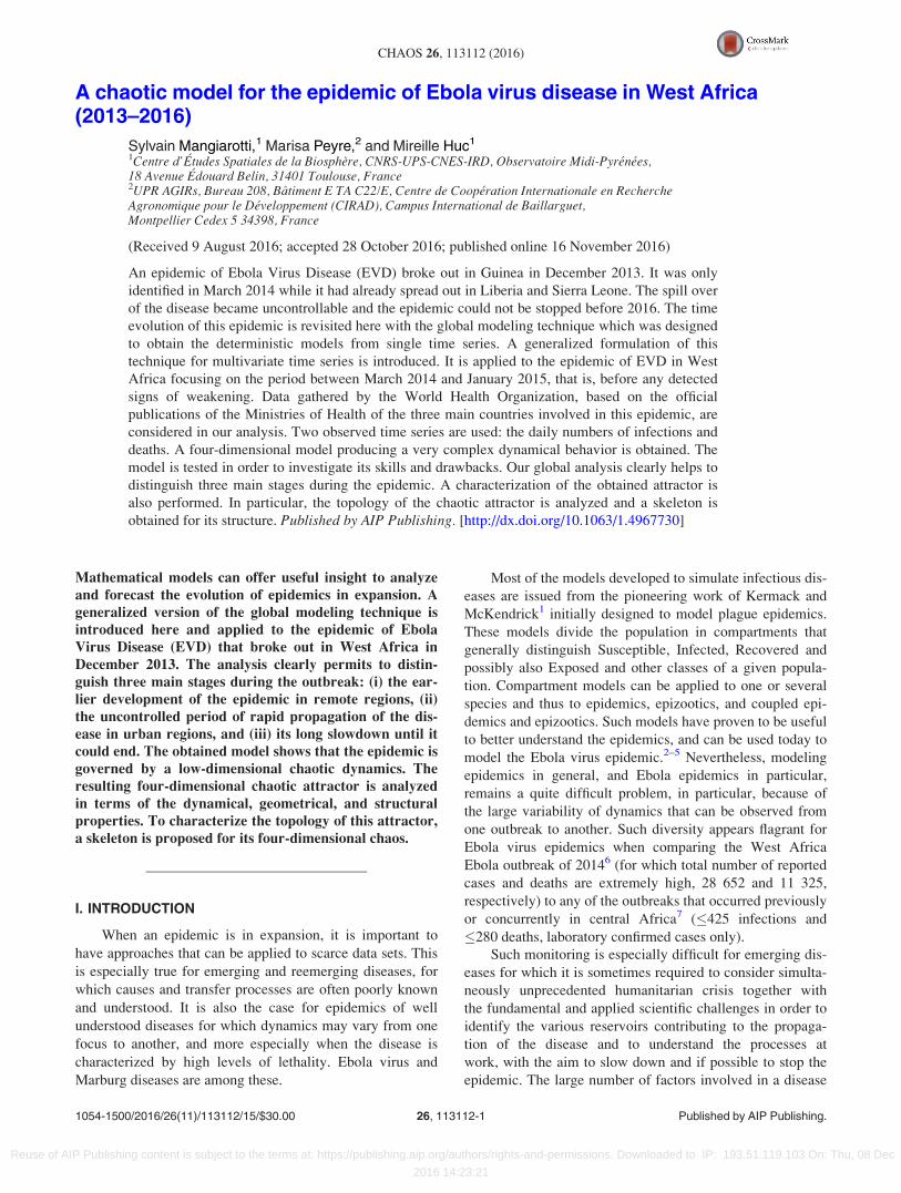
time (Fig. 1(a), dotted values). Since, almost all (>99:7 %)
Ebola cases of infections and deaths belong to the same geo-
graphical region (a large scale area including Guinea,
Liberia, and Sierra Leone), values basically resulting from
the addition of these three countries are used to perform the
analysis. The time window used for the modeling focuses on
year 2014, from the 23rd of March 2014 to the 21st of
January 2015 (from day 107 to day 411 after the index case
that was identified to take place on the 6th of December
2013;26 this date is the time reference of the epidemic used
in the manuscript).
This time window thus includes the mostly active period
of the epidemic, before any clear breakdown of the propaga-
tion could be detected. The evolution of the epidemics after
January 2015 and until January 20th 2016 (day 775) will not
be used for modeling but will be considered in the analysis
for discussion.
These data25 result from a real time data gathering pro-
cess and may thus include modifications induced by reclassi-
fications, new retrospective investigations, as well as time
delay that will depend on laboratories availability.27 For
these reasons, data may exhibit inconsistencies. In the pre-
sent case, some obvious contradictions were found quite
located in time and/or relatively moderated in magnitude.
Incoherences were fixed numerically by eliminating incon-
sistent values (corresponding to temporary decreases of
cumulative number of infections or deaths): values corre-
sponding to days 276, 320, 327, 329, 357, and 565 were thus
removed. A preprocessing was then applied as follows: the
two time series were re-sampled at a 1-day sampling using
cubic splines. A damping function was applied to bound the
negative values closer to zero. The curves obtained for X0
and Y0 are presented in Figure 1(a) (plain line).
Daily numbers of infected cases and deaths were
deduced from the previously preprocessed time series of
cumulative number by computing the derivatives. The
Savitzky-Golay filter28 was used for this purpose and deriva-
tives of higher degree, later required for applying the global
modeling technique, were computed at the meantime (Figure
1). The time series of the daily numbers Xobs1 of infections
and Yobs1 of deaths present a high level of complexity with
various time scales. The two variables Xobs1 and Yobs
1 have an
overall coherent coevolution although not always correlated.
Indeed, delayed oscillations and differentiated shapes and
amplitudes can clearly be observed along the temporal
signal. Their first and second derivatives are also reported
(Figs. 1(c) and 1(d)). Despite the inherent limits previously
evoked, the resulting time series appear coherent enough
to apply our global modeling technique introduced in
Section III.
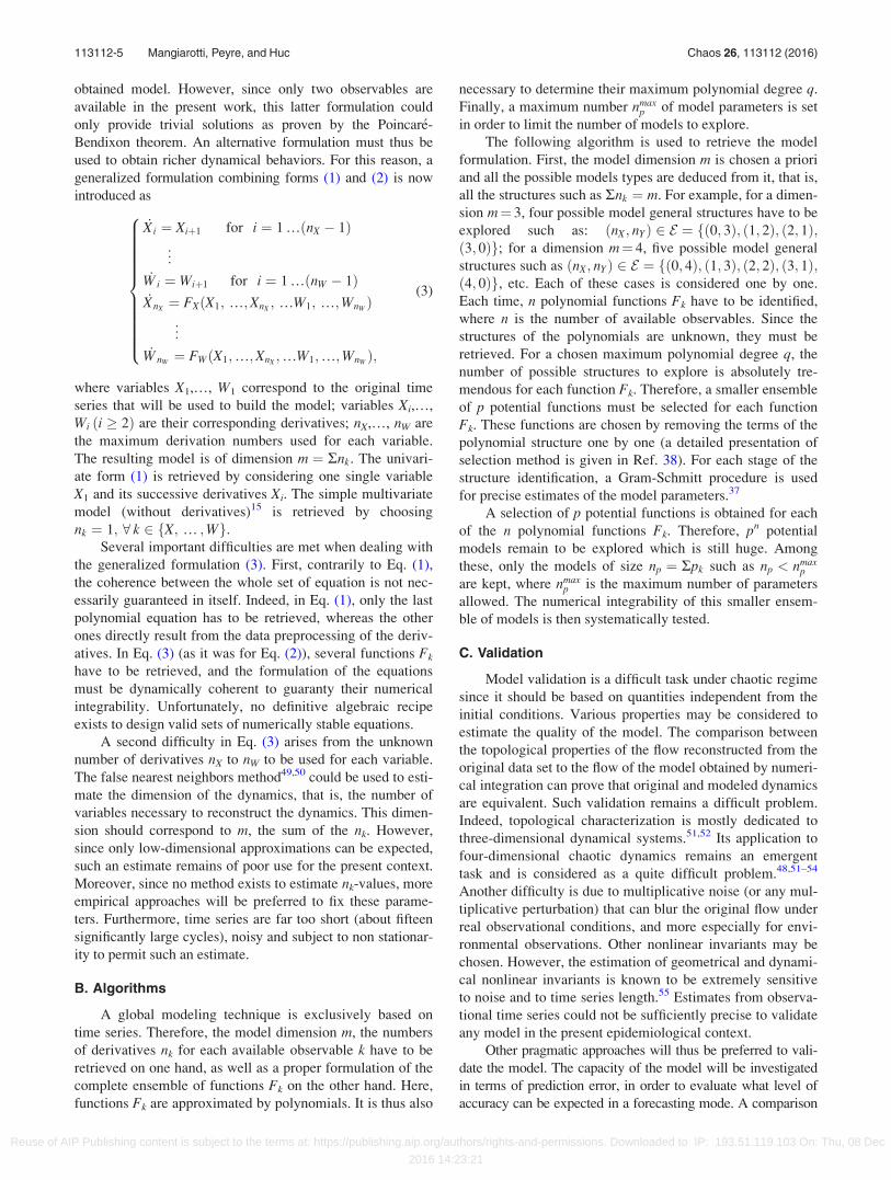
FIG. 1. Cumulative counts Xobs0 and Yobs
0 (a), daily numbers Xobs1 and Yobs
1
(b), and their first (c) and second (d) derivatives, of infections (in red) and
deaths (in black) due to EVD for the West Africa epidemic for the region
including Guinea, Liberia, and Sierra Leone. Date are given in day after the
index case corresponding to December, the 6th of 2013.26 Transitions
between the three stages are reported as vertical bands. (For more conve-
nience, note that January 1st corresponds to days 26 for 2014; 391 for 2015;
756 for 2016).
113112-3 Mangiarotti, Peyre, and Huc Chaos 26, 113112 (2016)
Reuse of AIP Publishing content is subject to the terms at: https://publishing.aip.org/authors/rights-and-permissions. Downloaded to IP: 193.51.119.103 On: Thu, 08 Dec
2016 14:23:21
D. Stages of the West Africa epidemic
Three main stages during the propagation of this disease
may be distinguished. The earlier stage (days� 0–220) corre-
sponds to a period of moderate but complex expansion of the
EVD in areas of low population density. Epidemiological
look-back investigations allowed the identification of an index
case who died on December 6th, 2013 in Meliandou, a small
village of Gu�eck�edou (Guinea).26 The retrospective analysis
revealed four linked clusters of infection and showed that the
disease may have been spread from Gu�eck�edou to Macenta
(103 km from it), Nz�er�ekor�e (237 km) and Kissidougou
(91 km) by a healthcare worker in February 2014.26 The vicin-
ity and the high porosity of the frontiers in the region, typical
of West Africa, permitted the transfer of the disease from
Guinea to Liberia and then to Sierra Leone. The hospitals and
public health services in Gu�eck�edou and Macenta (Guinea)
alerted the Ministry of Health of Guinea on March 10th, 2014
about an unidentified disease of apparent high fatality rate.
Blood samples were collected from hospitalized patients from
which Ebola virus was identified. Until July 2014, a complex
evolution of the epidemic in space and time was observed. In
particular, later starts of quicker increases of the number of
infections and deaths were noted in Liberia and Sierra
Leone.11 At this time, it seemed that the West Africa epidemic
was contained.
Several unexpected new foci were found during July
2014, the epidemic had been underestimated and had become
out of control. The second stage (days� 220–418) of the
West Africa epidemic of EVD had already started. The Ebola
Outbreak in West Africa was declared a “Public Health
Emergency of International Concern” by the Emergency
Committee in the beginning of August 2014.29 This emer-
gency was confirmed during the following weeks by an expo-
nential increase of infections and death counts at the end of
August (day� 265).30 The quick spill-over of the disease was
very likely due to a combination of problems that authorities
had to face during the spread of the disease:11 healthcare pro-
fessionals were not trained to manage suspected and con-
firmed cases; organization to trace contacts between possibly
affected individuals was not effective; resources and organiza-
tion to follow new outbreaks of infections were insufficient;
local community often exhibited a strong distrust towards
control and prevention teams, and sometimes skepticism or
even hostility, denying the access to medical teams. Since the
virus quickly spread out from one district to another, even
reaching numerous large cities including Conakry (Guinea) in
March 2014, Monrovia (Liberia) in April 2014, Freetown
(Sierra Leone) in July 2014 and others, new cases arose in
multiple locations. It became especially difficult for the
response team to follow all signaled cases and to trace them
back. After an exponential increase observed at the end of
August, the propagation speed reached the highest averaged
levels (Xobs1 > 100 infections per day) which maintained dur-
ing several months. The propagation rate appeared roughly
regular in average (considering the cumulative counts) reflect-
ing the relatively stationary conditions for the epidemiological
dynamics during this period. A slight slowdown of the epi-
demic was temporarily observed at day� 380 but this
detection remained local and uncertain at this date. Indeed,
although incidences were estimated to be stable or declining
in Liberia at the beginning of December (day 363),31 it
remained increasing in Guinea and Sierra Leone.32,33
It is only at the end of January 2015 that the focus could
be considered as shifting from “slowing the transmission to
ending the epidemic,”34 corresponding to the third stage of
the epidemic (day� 418-end). In practice, the limits between
the different stages are difficult to define precisely. A
decrease of strength was progressively observed. After day-
� 500, the number of deaths stabilized whereas the cumula-
tive number of cases continued to increase slowly. Both
variables almost completely stabilized after day� 700. The
end of the epidemic was declared on June 9th, 2016.
III. METHODOLOGY
A. The global modeling technique
The global modeling technique aims to obtain models
that can reproduce the global solutions of the dynamics,
directly from time series, that is, without any other a prioriinformation.35,36 It can be applied to retrieve the Ordinary
Differential Equations (ODE),37,38 discrete equations,39,40 or
delayed equations.36,41 In the present paper, only the contin-
uous case of ODE is considered. When a single observable is
available, the canonical form
_Xi ¼ Xiþ1 for i ¼ 1…ðn� 1Þ_Xn ¼ FðX1;X2;…;XnÞ;
((1)
can be used, where Xi represents the ði� 1Þ th derivative of
the observed variable X1 assumed to be linked to the original
variable x of the studied system such as X1 ¼ hðxÞ, with hthe measurement function assumed bijective and smooth.
Such an approach was successfully applied to numerous the-
oretical systems37,38,42 and to the experimental data as
well.38,43,44 A three-dimensional model was obtained for
lynx population in Canada.12 Two three-dimensional models
were obtained to model the cycles of cereal crops in North
Morocco.13 Interestingly, these latter models are the first
models to provide an example of weakly dissipative chaos in
nature. Indeed, all previous cases of weakly dissipative chaos
are theoretical models that had not been obtained from the
data.45–47 Other examples of weakly dissipative 3D chaos
were obtained for crops cycles in other Moroccan provin-
ces.48 These results contribute to prove that global modeling
technique can be applied to a large spectrum of dynamical
behaviors and to very different types of problems.
When several observables are available, the coupling
between the observed variables can directly be investigated.
In this case, the following form
_Xi ¼ FiðX1;X2;…;XnÞ for i ¼ 1…n; (2)
may be expected.15,48 Such formulation was shown to be a
powerful approach to identify the couplings of the epidemic
of plague in Bombay with the two epizootics of brown and
black rats15 by the end of 19th century. Surprisingly, it was
found even possible to give a full interpretation of the
113112-4 Mangiarotti, Peyre, and Huc Chaos 26, 113112 (2016)
Reuse of AIP Publishing content is subject to the terms at: https://publishing.aip.org/authors/rights-and-permissions. Downloaded to IP: 193.51.119.103 On: Thu, 08 Dec
2016 14:23:21
obtained model. However, since only two observables are
available in the present work, this latter formulation could
only provide trivial solutions as proven by the Poincar�e-
Bendixon theorem. An alternative formulation must thus be
used to obtain richer dynamical behaviors. For this reason, a
generalized formulation combining forms (1) and (2) is now
introduced as
_Xi ¼ Xiþ1 for i ¼ 1 …ðnX � 1Þ...
_Wi ¼ Wiþ1 for i ¼ 1 …ðnW � 1Þ_XnX¼ FXðX1; …;XnX
; …W1; …;WnWÞ
..
.
_WnW ¼ FWðX1;…;XnX ;…W1;…;WnW Þ;
8>>>>>>>>>>><>>>>>>>>>>>:
(3)
where variables X1,…, W1 correspond to the original time
series that will be used to build the model; variables Xi,…,
Wi ði � 2Þ are their corresponding derivatives; nX,…, nW are
the maximum derivation numbers used for each variable.
The resulting model is of dimension m ¼ Rnk. The univari-
ate form (1) is retrieved by considering one single variable
X1 and its successive derivatives Xi. The simple multivariate
model (without derivatives)15 is retrieved by choosing
nk ¼ 1; 8 k 2 fX; … ;Wg.Several important difficulties are met when dealing with
the generalized formulation (3). First, contrarily to Eq. (1),
the coherence between the whole set of equation is not nec-
essarily guaranteed in itself. Indeed, in Eq. (1), only the last
polynomial equation has to be retrieved, whereas the other
ones directly result from the data preprocessing of the deriv-
atives. In Eq. (3) (as it was for Eq. (2)), several functions Fk
have to be retrieved, and the formulation of the equations
must be dynamically coherent to guaranty their numerical
integrability. Unfortunately, no definitive algebraic recipe
exists to design valid sets of numerically stable equations.
A second difficulty in Eq. (3) arises from the unknown
number of derivatives nX to nW to be used for each variable.
The false nearest neighbors method49,50 could be used to esti-
mate the dimension of the dynamics, that is, the number of
variables necessary to reconstruct the dynamics. This dimen-
sion should correspond to m, the sum of the nk. However,
since only low-dimensional approximations can be expected,
such an estimate remains of poor use for the present context.
Moreover, since no method exists to estimate nk-values, more
empirical approaches will be preferred to fix these parame-
ters. Furthermore, time series are far too short (about fifteen
significantly large cycles), noisy and subject to non stationar-
ity to permit such an estimate.
B. Algorithms
A global modeling technique is exclusively based on
time series. Therefore, the model dimension m, the numbers
of derivatives nk for each available observable k have to be
retrieved on one hand, as well as a proper formulation of the
complete ensemble of functions Fk on the other hand. Here,
functions Fk are approximated by polynomials. It is thus also
necessary to determine their maximum polynomial degree q.
Finally, a maximum number nmaxp of model parameters is set
in order to limit the number of models to explore.
The following algorithm is used to retrieve the model
formulation. First, the model dimension m is chosen a priori
and all the possible models types are deduced from it, that is,
all the structures such as Rnk ¼ m. For example, for a dimen-
sion m¼ 3, four possible model general structures have to be
explored such as: ðnX; nYÞ 2 E ¼ fð0; 3Þ; ð1; 2Þ; ð2; 1Þ;ð3; 0Þg; for a dimension m¼ 4, five possible model general
structures such as ðnX; nYÞ 2 E ¼ fð0; 4Þ; ð1; 3Þ; ð2; 2Þ; ð3; 1Þ;ð4; 0Þg, etc. Each of these cases is considered one by one.
Each time, n polynomial functions Fk have to be identified,
where n is the number of available observables. Since the
structures of the polynomials are unknown, they must be
retrieved. For a chosen maximum polynomial degree q, the
number of possible structures to explore is absolutely tre-
mendous for each function Fk. Therefore, a smaller ensemble
of p potential functions must be selected for each function
Fk. These functions are chosen by removing the terms of the
polynomial structure one by one (a detailed presentation of
selection method is given in Ref. 38). For each stage of the
structure identification, a Gram-Schmitt procedure is used
for precise estimates of the model parameters.37
A selection of p potential functions is obtained for each
of the n polynomial functions Fk. Therefore, pn potential
models remain to be explored which is still huge. Among
these, only the models of size np ¼ Rpk such as np < nmaxp
are kept, where nmaxp is the maximum number of parameters
allowed. The numerical integrability of this smaller ensem-
ble of models is then systematically tested.
C. Validation
Model validation is a difficult task under chaotic regime
since it should be based on quantities independent from the
initial conditions. Various properties may be considered to
estimate the quality of the model. The comparison between
the topological properties of the flow reconstructed from the
original data set to the flow of the model obtained by numeri-
cal integration can prove that original and modeled dynamics
are equivalent. Such validation remains a difficult problem.
Indeed, topological characterization is mostly dedicated to
three-dimensional dynamical systems.51,52 Its application to
four-dimensional chaotic dynamics remains an emergent
task and is considered as a quite difficult problem.48,51–54
Another difficulty is due to multiplicative noise (or any mul-
tiplicative perturbation) that can blur the original flow under
real observational conditions, and more especially for envi-
ronmental observations. Other nonlinear invariants may be
chosen. However, the estimation of geometrical and dynami-
cal nonlinear invariants is known to be extremely sensitive
to noise and to time series length.55 Estimates from observa-
tional time series could not be sufficiently precise to validate
any model in the present epidemiological context.
Other pragmatic approaches will thus be preferred to vali-
date the model. The capacity of the model will be investigated
in terms of prediction error, in order to evaluate what level of
accuracy can be expected in a forecasting mode. A comparison
113112-5 Mangiarotti, Peyre, and Huc Chaos 26, 113112 (2016)
Reuse of AIP Publishing content is subject to the terms at: https://publishing.aip.org/authors/rights-and-permissions. Downloaded to IP: 193.51.119.103 On: Thu, 08 Dec
2016 14:23:21
between the variables of the original data and of the model out-
put, and their distributions, will also be performed.
It is important to point out that obtaining a global model
producing a flow more developed than the original one is com-
mon.48,56 In fact, this is one of its goal, and this is why global
modeling is well adapted for modeling chaos. It is designed—
in its principle—to retrieve the equations for the vector field.
When the equations are accurately retrieved, they are able to
produce the full set of possible solutions and not only the par-
ticular solutions from which the global model was obtained.
Nevertheless, altered behaviors may arise due to noisy
conditions36 and to data aggregation10 which may perturb
the selection of the model structure. The lack of observabil-
ity57,58 is another important source of difficulty that may
blur—or sometimes even hinder—the model identification.
Nonetheless, extreme trajectories, although never visited in
the original data sets, may be retrieved and can be signifi-
cant. Theoretically, the global modeling can thus provide
useful elements to investigate extreme events without any
strong hypotheses about the model dynamics or about the
tail of the probability function.
IV. RESULTS AND DISCUSSIONS
A. Phase portraits
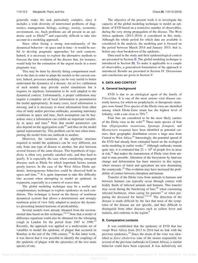
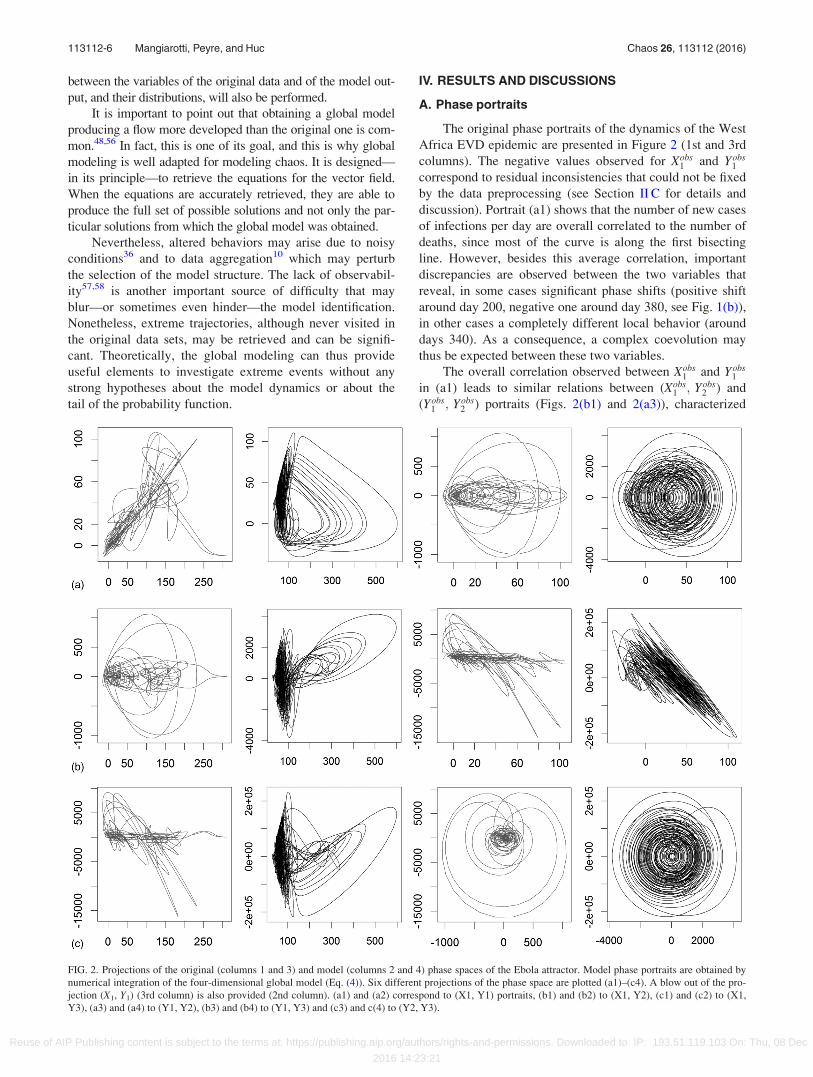
The original phase portraits of the dynamics of the West
Africa EVD epidemic are presented in Figure 2 (1st and 3rd
columns). The negative values observed for Xobs1 and Yobs
1
correspond to residual inconsistencies that could not be fixed
by the data preprocessing (see Section II C for details and
discussion). Portrait (a1) shows that the number of new cases
of infections per day are overall correlated to the number of
deaths, since most of the curve is along the first bisecting
line. However, besides this average correlation, important
discrepancies are observed between the two variables that
reveal, in some cases significant phase shifts (positive shift
around day 200, negative one around day 380, see Fig. 1(b)),
in other cases a completely different local behavior (around
days 340). As a consequence, a complex coevolution may
thus be expected between these two variables.
The overall correlation observed between Xobs1 and Yobs
1
in (a1) leads to similar relations between (Xobs1 ; Yobs
2 ) and
(Yobs1 ; Yobs
2 ) portraits (Figs. 2(b1) and 2(a3)), characterized
FIG. 2. Projections of the original (columns 1 and 3) and model (columns 2 and 4) phase spaces of the Ebola attractor. Model phase portraits are obtained by
numerical integration of the four-dimensional global model (Eq. (4)). Six different projections of the phase space are plotted (a1)–(c4). A blow out of the pro-
jection (X1, Y1) (3rd column) is also provided (2nd column). (a1) and (a2) correspond to (X1, Y1) portraits, (b1) and (b2) to (X1, Y2), (c1) and (c2) to (X1,
Y3), (a3) and (a4) to (Y1, Y2), (b3) and (b4) to (Y1, Y3) and (c3) and c(4) to (Y2, Y3).
113112-6 Mangiarotti, Peyre, and Huc Chaos 26, 113112 (2016)
Reuse of AIP Publishing content is subject to the terms at: https://publishing.aip.org/authors/rights-and-permissions. Downloaded to IP: 193.51.119.103 On: Thu, 08 Dec
2016 14:23:21
by numerous extended trajectories along the abscissa and a
few circular ones. For the same reason, similarities are
observed between (Xobs1 ; Yobs
3 ) and (Yobs1 ; Yobs
3 ) portraits
(Figs. 2(c1) and 2(b3)). For these two projections, most of
the trajectories have a long extension along the abscissa
whereas a few trajectories exhibit a curved diagonal pattern.
Finally, the last portrait (Yobs2 ; Yobs
3 ) in (c3) exhibits cardioid-
like structures of irregular amplitudes.
B. A four-dimensional model
The procedure described in Section III B was applied to
the window from day 107 to day 411, including the period of
rapid progression of the epidemic (see Section II D). Models of
dimension m¼ 3 to 5 were investigated for maximum polyno-
mial degrees q¼ 2 to 3 and for maximum size (the parameter
maximum number) nmaxp ¼ 20. The very most of the obtained
models were either numerically non integrable, either diver-
gent, or converging to a trivial solution (among these latter,
exclusively period-1 cycles were obtained for the present data-
set). It may be useful to note that, when unsuccessful, the gen-
eral formulations revealed quite different levels of inadequacy:
most of the formulations among ensembles E (see Section
III B) led to immediate and systematic model rejection (models
completely non integrable), whereas few formulations showed
to be numerically integrable for long testing periods although
finally diverging and thus leading to rejection.
Finally, a single non-trivial integrable model was
obtained. This model is a 4-dimensional model (such as
nX¼ 1 and nY¼ 3) producing an attractor of complex struc-
ture. This model reads
_X1 ¼ a1Y1Y3 þ a2Y21 � a3X1Y1
_Y1 ¼ Y2
_Y2 ¼ Y3
_Y3 ¼ b1 þ bb2Y3 þ b3Y23 � b4Y2 � b5Y2
2 þ b6Y1
�b7Y1Y3 þ b8Y1Y2 � b9Y21 � b10X1
�b11X1Y3 � b12X1Y2 þ b13X1Y1 þ b14X21;
8>>>>>>>>><>>>>>>>>>:
(4)
where parameters ai and bi are reported in Table I. The
parameter b is a tuning parameter such as b¼ 1 by default.
This 4D model provides a strong argument for determinism,
and, more precisely, for a low-dimensional determinism
overriding the dynamics of this epidemic.
The detection of such low-dimensional deterministic
model suggests that societal and environmental conditions
were quite conducive to the propagation of the epidemic:
once the epidemic had broken out, its propagation was
largely determined, and probably driven by predominant pro-
cesses, and possibly few ones.
The obtained model has four fixed points
Q1ða1; 0; 0; 0Þ; Q2ða2; 0; 0; 0Þ;Q3ða3; a03; 0; 0Þ and Q4ða4; a04; 0; 0Þ;
(5)
with a1 � 99:403; a2 � 0:325, a3 � �0:240; a03 � �0:167,
a4 � 198:194 and a04 � 137:634. Their classification can be
deduced from the eigenvalues KQiof the Jacobian matrix J
linearized at their location Qi (see supplementary material
for details).
For Q1, two sets of conjugate complex numbers are
obtained such as KQ1¼ ðc1 þ d1i; c1 � d1i; e1 þ f1i;
e1 � f1iÞ, with real components c1 < 0 and e1 > 0. This
point is thus a double-focus point, one focus being stable, the
other being unstable.
For Q2, one set of conjugate complex eigenvalues and
two real eigenvalues are obtained such as KQ2¼ ðc2 þ d2i;
c2 � d2i; e2; g2Þ, with c2 < 0; e2 > 0 and g2 < 0. This is
thus a focus-saddle point.
For Q3 and Q4, only real eigenvalues are obtained such
as KQ3¼ ðc3; d3; e3; g3Þ and KQ4
¼ ðc4; d4; e4; g4Þ. These
points are both saddle points. Only one single direction is
stable for Q3 since only c3 < 0. This point will not have a
direct signification since its location corresponds to negative
values of X1 and Y1. Two directions are stable for Q4 since
both e4 < 0 and g4 < 0.
The attractor obtained from Eq. (4) is shown in Figure 2
(columns 2 and 4) for various projections (transients were
removed). The attractor exhibits a quite complex behavior. A
region of the phase space of “triangular” shape (left of X1Y1-
plane projections, Figs. 2(a2)–2(c2)) with a high density of tra-
jectories. Oscillations in this region are relatively moderated in
amplitude (Xmax1 �140). The observational data mostly belongs
to this domain of the phase space (see Fig. 2, 1st column).
The other part of the attractor is associated with larger
oscillations of variable X1 which are quite sparse and are not
observed in the original portrait (Fig. 2, 1st column). Quite
extreme values of X1 are obtained in the simulations, up to
600 infections per day. Very punctually these can reach
values up to 1200 infections per day with longer simulations.
Contrary to this, the largest values reached by Y1 are almost
never beyond 175 deaths per day.
Some patterns can be retrieved in both observed and
modeled portraits. In (a2), the linear relation observed in
(a1) between Xobs1 and Yobs
1 in the “triangular” region is
retrieved, despite a significantly steeper slope obtained. The
rare anti-correlated trajectories observed in the original por-
trait are likely to correspond to the other type of oscillations
which do not belong to the “triangular” region. In the simula-
tions, these can have very large amplitudes along X1 axis as
observed in (a2). In (b2) and (c2), both extended and circular
trajectories observed in (b1) and (c1) are more or less
retrieved, although strongly altered in shape. In (a4) and
(b4), the extended trajectories observed in (a4) and (b3)
along Yobs1 axis are difficult to identify, especially in (b4).
Contrarily, circular trajectories in (a3), and diagonal ones in
(b3) are clearly retrieved in (a4) and (b4). Finally, a good
TABLE I. Parameter values ai and bi for the four-dimensional global model
(Eq. (4)). By default, b is equal to 1.
a1 1.0894896 10�4 b4 1921.271852 b10 17867.66051
a2 1.4135051035 b5 0.1614398401 b11 0.06616088061
a3 0.9815931187 b6 34650.56048 b12 24.91575291
b1 5791.076327 b7 0.057295177 b13 300.3855818
b2 3.744720590 b8 14.52947493 b14 179.1636118
b3 2.2511395 10�5 b9 1056.142579
113112-7 Mangiarotti, Peyre, and Huc Chaos 26, 113112 (2016)
Reuse of AIP Publishing content is subject to the terms at: https://publishing.aip.org/authors/rights-and-permissions. Downloaded to IP: 193.51.119.103 On: Thu, 08 Dec
2016 14:23:21
coherency is observed between (c3) and (c4), for which
cardioid-like patterns can be observed in both portraits.
The spectrum of Lyapunov exponents59 of the model
dynamics was estimated. Their values clearly reveal the high
sensitivity of the dynamics to initial conditions (k1 � 0):
k1 ¼ 2:6260:03; k2 ¼ 0:0260:03; k3 ¼ �1:8760:03; k4
¼ �30:260:06Þ. The two necessary conditions—determin-
ism, and high sensitivity to initial conditions—are thus
retrieved together in a synthetic formulation (Eq. (4)) and
provide a strong argument for a low-dimensional chaotic
underlying dynamics. As seen in a (X1, Y1)-portrait, close
trajectories at low values of infection (at the beginning of
new flare-up episode) tend to diverge; and tend to converge
at the end of each episode. The closeness of the trajectories at
the beginning of new flare-ups suggests that actions for slow-
ing down the propagation of the disease (by avoiding or mini-
mizing its transmission at the earliest stages of the infections)
can be of high efficacy. This observation is in full agreement
with the preventive and control measures put in place by the
health community to trace back the cases of infections and
deaths to prevent the dissemination of the disease. It also
strengthens the importance not to leave any detected case of
infection or death under careful observation and control.
The spectrum of Lyapunov exponents can also be used
to estimate the fractal dimension of the attractor.60 This
invariant was proven to be well adapted to global model-
ing.13 The Kaplan-Yorke dimension is defined as
DKY ¼ k þ
Pki¼1
ki
jkkþ1j; (6)
where k is the maximum value such asPk
i¼1 ki > 0. In the
present case we get DKY � 3:03. The Ebola attractor is thus
clearly four-dimensional but strongly dissipative since DKY
is such as d � 1 < DKY d, where d¼ 4 is the model
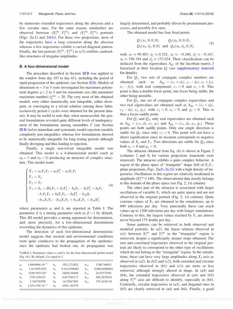
dimension. To characterize the structure of the attractor, the
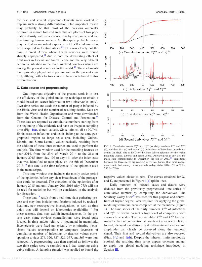
Poincar�e section
P ¼ fðX1; Y1; Y3Þ 2 A R4=Y2 ¼ 0; Y3 < 0g; (7)
was chosen, where A designates the Ebola attractor. The
resulting section is plotted in Figure 3(a). A first return map is
usually used to distinguish folding from tearing mechanisms in
chaotic attractors.52,61 To do so, the map is expected to be
surjective which is completely impossible for a three-
dimensional Poincar�e section. To analyze the first return map
of the section P plotted in Figure 3(a), an alternate approach
based on color tracer is used.48 To simplify the visualization of
the underlying structure, the diffeomorphism
~X1 ¼ X1; ~Y1 ¼ Y2; ~Y3 ¼ Y3 þ 2500 Y1; (8)
is first applied to section P (Eq. (7)), leading to section ~P. To
analyze the first return mapping of this section to itself, a
color tracer is applied at time t. Its representation ~Pt is shown
in Figure 3(c). Color tracers are then propagated backward
into ~Pt�1 (Fig. 3(b)) and forward into ~Ptþ1 and ~Ptþ2 (Figs.
3(d) and 3(e)). The existence conditions for a suspension
states that, for a section in Rm, the suspension should be in
Rm� with either m� ¼ mþ 1 or m� ¼ mþ 2.48,54 Since m and
m� are known here (m¼ 3 and m� ¼ 4), the model structure
should be represented as a branched 3D-manifold embedded
in a four-dimensional space. To distinguish it from the so
called template (a branched 2D-manifold embedded in a 3D
space), this structure will be called a “skeleton”.
The visual analysis of the transition from ~Pt�1 to ~Pt pro-
vides most of the information about the mapping.48 First, the
continuous limit between the light green (noted A1) and the
light red (noted B) in ~Pt�1 becomes discontinuous (A01 and
B0) in ~Pt: it reveals the presence of a tearing mechanism in
the attractor. The torn branch (A) becomes the two folded
branches (A01) and (A02). One goes to the upper side of the
section, the other one to its lower side. A torsion clearly
takes place between A01 and A02 as indicated by the normal
vectors to the two surfaces (~n1 and ~n2) from the initial sec-
tion, to the next return (~n01 and ~n02). Second, branch (B)
replaces branch (A). The transition from ~Pt to ~Ptþ1 mostly
shows that branch (A01) becomes (A001), whereas transition
from (B0) to (B00) just confirms the behavior revealed by (A).
The transition from ~Ptþ1 to ~Ptþ2 enables to illustrate the suc-
cessive accumulation of branches issuing from region A2 on
the top of the structure (C000, A0001, B0001, etc.).
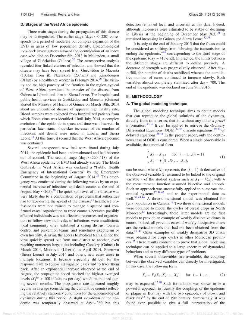
Based on these observations, a four-branch structure of
the Ebola attractor is sketched in Figure 4(a), showing the
successive transformations of the section ~P to come back to
itself in a space tangent to the attractor in the phase space.
Four branches are necessary to characterize the attractor that
FIG. 3. (a) Poincar�e section P to the Ebola attractor A (its definition is given in Eq. (7)). Colored values in (a) aim to better distinguish the 3D shape of the sec-
tion. Section ~P diffeomorphic to section P based on Eq. (8) is also presented at different times using a color tracer that is propagated from one section to the
next return: ~Pt�1 in (b), ~Pt in (c), ~Pt in (d) and ~Ptþ2 in (e). To facilitate the analysis, three main regions noted A1, A2, and B are selected in ~Pt�1. Their propaga-
tions are noted with simple and multiple primes in ~Pt and next ~Ptþ1 and ~Ptþ2. Two arrows provide the normal to regions A1 and A2 and their propagation in
their next return in order to clearly illustrate the foldings, one remaining visible, another one disappearing inside the section.
113112-8 Mangiarotti, Peyre, and Huc Chaos 26, 113112 (2016)
Reuse of AIP Publishing content is subject to the terms at: https://publishing.aip.org/authors/rights-and-permissions. Downloaded to IP: 193.51.119.103 On: Thu, 08 Dec
2016 14:23:21
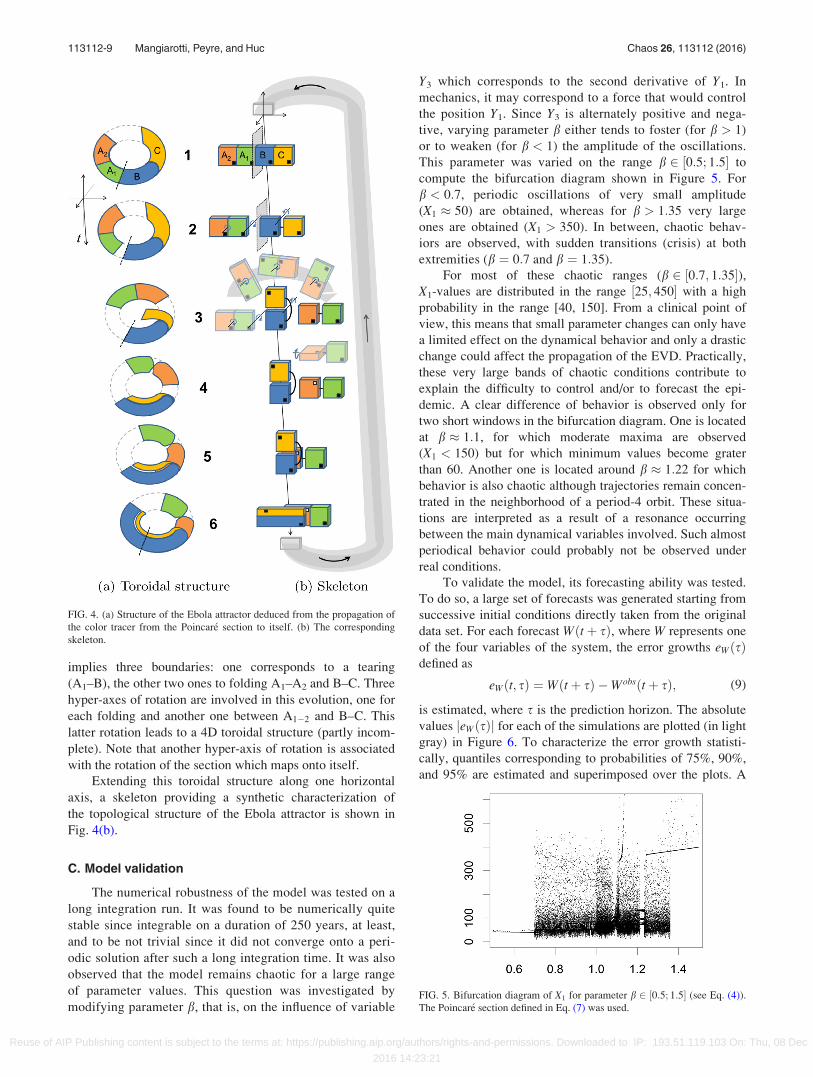
implies three boundaries: one corresponds to a tearing
(A1–B), the other two ones to folding A1–A2 and B–C. Three
hyper-axes of rotation are involved in this evolution, one for
each folding and another one between A1�2 and B–C. This
latter rotation leads to a 4D toroidal structure (partly incom-
plete). Note that another hyper-axis of rotation is associated
with the rotation of the section which maps onto itself.
Extending this toroidal structure along one horizontal
axis, a skeleton providing a synthetic characterization of
the topological structure of the Ebola attractor is shown in
Fig. 4(b).
C. Model validation
The numerical robustness of the model was tested on a
long integration run. It was found to be numerically quite
stable since integrable on a duration of 250 years, at least,
and to be not trivial since it did not converge onto a peri-
odic solution after such a long integration time. It was also
observed that the model remains chaotic for a large range
of parameter values. This question was investigated by
modifying parameter b, that is, on the influence of variable
Y3 which corresponds to the second derivative of Y1. In
mechanics, it may correspond to a force that would control
the position Y1. Since Y3 is alternately positive and nega-
tive, varying parameter b either tends to foster (for b > 1)
or to weaken (for b < 1) the amplitude of the oscillations.
This parameter was varied on the range b 2 ½0:5; 1:5� to
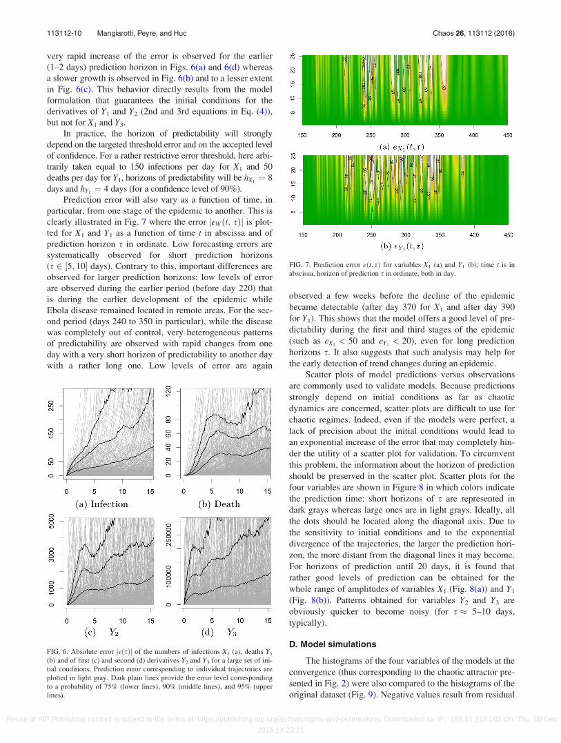
compute the bifurcation diagram shown in Figure 5. For
b < 0:7, periodic oscillations of very small amplitude
(X1 � 50) are obtained, whereas for b > 1:35 very large
ones are obtained (X1 > 350). In between, chaotic behav-
iors are observed, with sudden transitions (crisis) at both
extremities (b ¼ 0:7 and b ¼ 1:35).
For most of these chaotic ranges (b 2 ½0:7; 1:35�),X1-values are distributed in the range ½25; 450� with a high
probability in the range [40, 150]. From a clinical point of
view, this means that small parameter changes can only have
a limited effect on the dynamical behavior and only a drastic
change could affect the propagation of the EVD. Practically,
these very large bands of chaotic conditions contribute to
explain the difficulty to control and/or to forecast the epi-
demic. A clear difference of behavior is observed only for
two short windows in the bifurcation diagram. One is located
at b � 1:1, for which moderate maxima are observed
(X1 < 150) but for which minimum values become grater
than 60. Another one is located around b � 1:22 for which
behavior is also chaotic although trajectories remain concen-
trated in the neighborhood of a period-4 orbit. These situa-
tions are interpreted as a result of a resonance occurring
between the main dynamical variables involved. Such almost
periodical behavior could probably not be observed under
real conditions.
To validate the model, its forecasting ability was tested.
To do so, a large set of forecasts was generated starting from
successive initial conditions directly taken from the original
data set. For each forecast Wðtþ sÞ, where W represents one
of the four variables of the system, the error growths eWðsÞdefined as
eWðt; sÞ ¼ Wðtþ sÞ �Wobsðtþ sÞ; (9)
is estimated, where s is the prediction horizon. The absolute
values jeWðsÞj for each of the simulations are plotted (in light
gray) in Figure 6. To characterize the error growth statisti-
cally, quantiles corresponding to probabilities of 75%, 90%,
and 95% are estimated and superimposed over the plots. A
FIG. 4. (a) Structure of the Ebola attractor deduced from the propagation of
the color tracer from the Poincar�e section to itself. (b) The corresponding
skeleton.
FIG. 5. Bifurcation diagram of X1 for parameter b 2 ½0:5; 1:5� (see Eq. (4)).
The Poincar�e section defined in Eq. (7) was used.
113112-9 Mangiarotti, Peyre, and Huc Chaos 26, 113112 (2016)
Reuse of AIP Publishing content is subject to the terms at: https://publishing.aip.org/authors/rights-and-permissions. Downloaded to IP: 193.51.119.103 On: Thu, 08 Dec
2016 14:23:21
very rapid increase of the error is observed for the earlier
(1–2 days) prediction horizon in Figs. 6(a) and 6(d) whereas
a slower growth is observed in Fig. 6(b) and to a lesser extent
in Fig. 6(c). This behavior directly results from the model
formulation that guarantees the initial conditions for the
derivatives of Y1 and Y2 (2nd and 3rd equations in Eq. (4)),
but not for X1 and Y3.
In practice, the horizon of predictability will strongly
depend on the targeted threshold error and on the accepted level
of confidence. For a rather restrictive error threshold, here arbi-
trarily taken equal to 150 infections per day for X1 and 50
deaths per day for Y1, horizons of predictability will be hX1¼ 8
days and hY1¼ 4 days (for a confidence level of 90%).
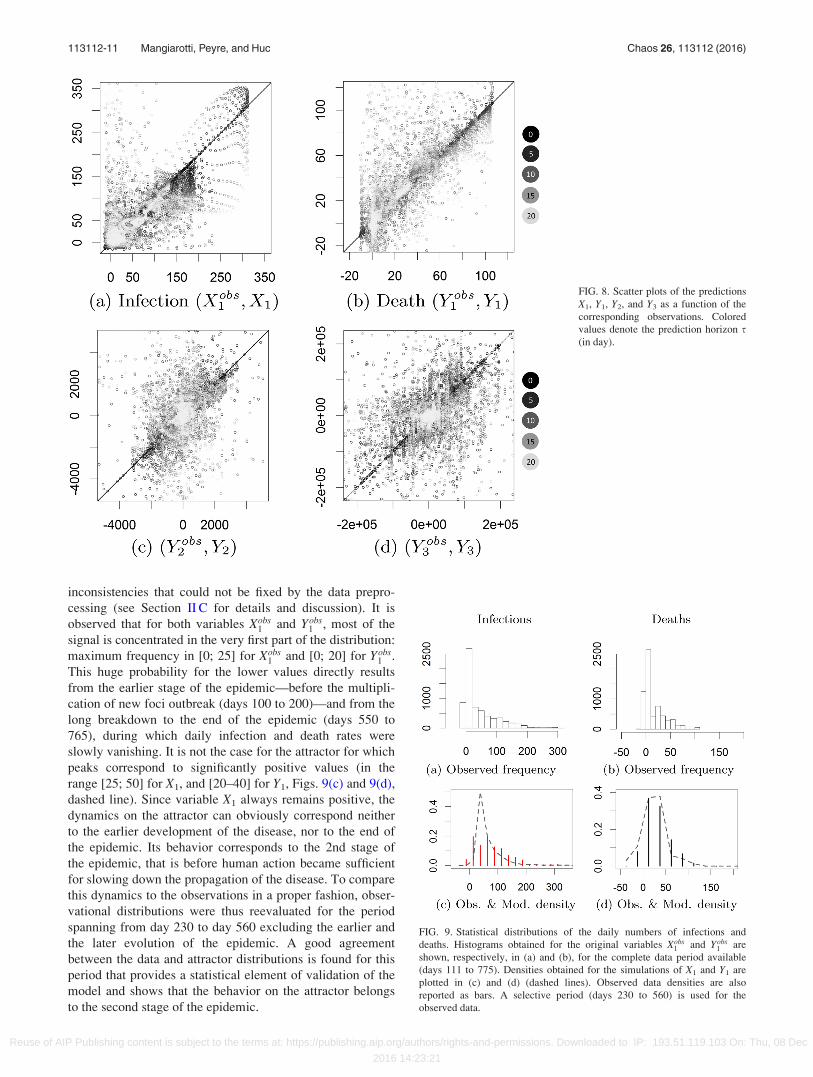
Prediction error will also vary as a function of time, in
particular, from one stage of the epidemic to another. This is
clearly illustrated in Fig. 7 where the error jeWðt; sÞj is plot-
ted for X1 and Y1 as a function of time t in abscissa and of
prediction horizon s in ordinate. Low forecasting errors are
systematically observed for short prediction horizons
(s 2 ½5; 10� days). Contrary to this, important differences are
observed for larger prediction horizons: low levels of error
are observed during the earlier period (before day 220) that
is during the earlier development of the epidemic while
Ebola disease remained located in remote areas. For the sec-
ond period (days 240 to 350 in particular), while the disease
was completely out of control, very heterogeneous patterns
of predictability are observed with rapid changes from one
day with a very short horizon of predictability to another day
with a rather long one. Low levels of error are again
observed a few weeks before the decline of the epidemic
became detectable (after day 370 for X1 and after day 390
for Y1). This shows that the model offers a good level of pre-
dictability during the first and third stages of the epidemic
(such as eX1< 50 and eY1
< 20), even for long prediction
horizons s. It also suggests that such analysis may help for
the early detection of trend changes during an epidemic.
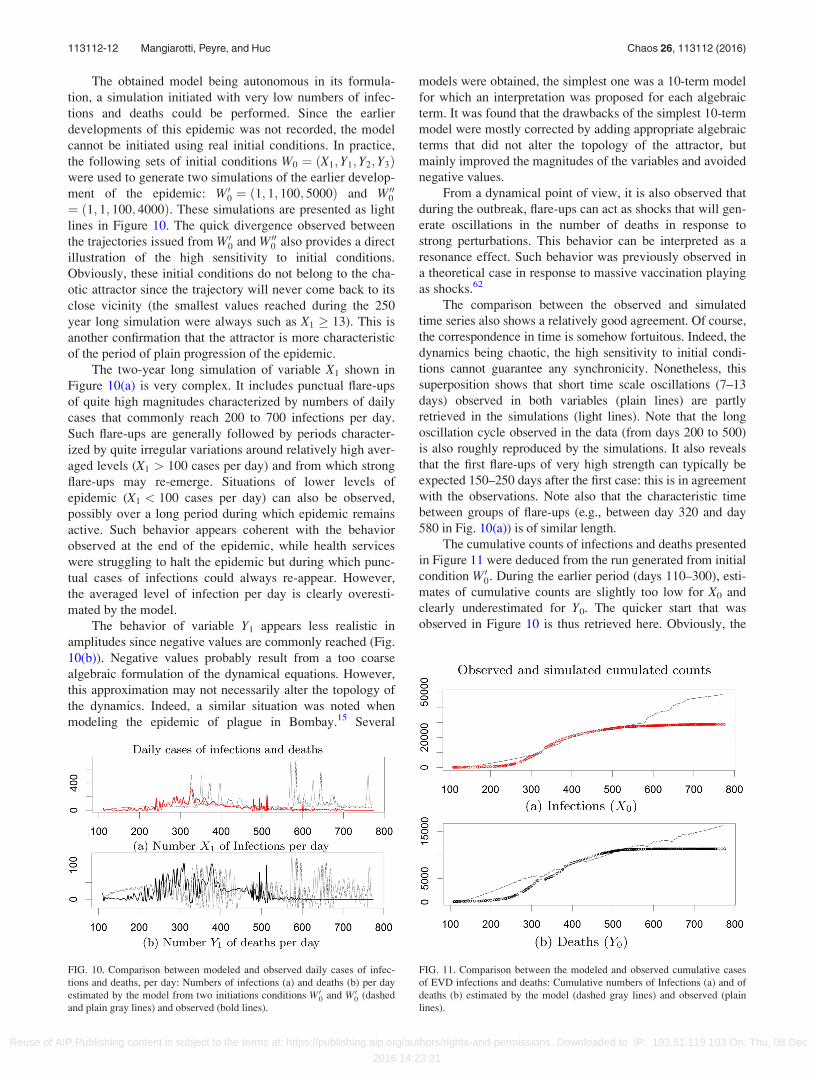
Scatter plots of model predictions versus observations
are commonly used to validate models. Because predictions
strongly depend on initial conditions as far as chaotic
dynamics are concerned, scatter plots are difficult to use for
chaotic regimes. Indeed, even if the models were perfect, a
lack of precision about the initial conditions would lead to
an exponential increase of the error that may completely hin-
der the utility of a scatter plot for validation. To circumvent
this problem, the information about the horizon of prediction
should be preserved in the scatter plot. Scatter plots for the
four variables are shown in Figure 8 in which colors indicate
the prediction time: short horizons of s are represented in
dark grays whereas large ones are in light grays. Ideally, all
the dots should be located along the diagonal axis. Due to
the sensitivity to initial conditions and to the exponential
divergence of the trajectories, the larger the prediction hori-
zon, the more distant from the diagonal lines it may become.
For horizons of prediction until 20 days, it is found that
rather good levels of prediction can be obtained for the
whole range of amplitudes of variables X1 (Fig. 8(a)) and Y1
(Fig. 8(b)). Patterns obtained for variables Y2 and Y3 are
obviously quicker to become noisy (for s � 5–10 days,
typically).
D. Model simulations
The histograms of the four variables of the models at the
convergence (thus corresponding to the chaotic attractor pre-
sented in Fig. 2) were also compared to the histograms of the
original dataset (Fig. 9). Negative values result from residual
FIG. 6. Absolute error jeðsÞj of the numbers of infections X1 (a), deaths Y1
(b) and of first (c) and second (d) derivatives Y2 and Y3 for a large set of ini-
tial conditions. Prediction error corresponding to individual trajectories are
plotted in light gray. Dark plain lines provide the error level corresponding
to a probability of 75% (lower lines), 90% (middle lines), and 95% (upper
lines).
FIG. 7. Prediction error eðt; sÞ for variables X1 (a) and Y1 (b); time t is in
abscissa, horizon of prediction s in ordinate, both in day.
113112-10 Mangiarotti, Peyre, and Huc Chaos 26, 113112 (2016)
Reuse of AIP Publishing content is subject to the terms at: https://publishing.aip.org/authors/rights-and-permissions. Downloaded to IP: 193.51.119.103 On: Thu, 08 Dec
2016 14:23:21
inconsistencies that could not be fixed by the data prepro-
cessing (see Section II C for details and discussion). It is
observed that for both variables Xobs1 and Yobs
1 , most of the
signal is concentrated in the very first part of the distribution:
maximum frequency in [0; 25] for Xobs1 and [0; 20] for Yobs
1 .
This huge probability for the lower values directly results
from the earlier stage of the epidemic—before the multipli-
cation of new foci outbreak (days 100 to 200)—and from the
long breakdown to the end of the epidemic (days 550 to
765), during which daily infection and death rates were
slowly vanishing. It is not the case for the attractor for which
peaks correspond to significantly positive values (in the
range [25; 50] for X1, and [20–40] for Y1, Figs. 9(c) and 9(d),
dashed line). Since variable X1 always remains positive, the
dynamics on the attractor can obviously correspond neither
to the earlier development of the disease, nor to the end of
the epidemic. Its behavior corresponds to the 2nd stage of
the epidemic, that is before human action became sufficient
for slowing down the propagation of the disease. To compare
this dynamics to the observations in a proper fashion, obser-
vational distributions were thus reevaluated for the period
spanning from day 230 to day 560 excluding the earlier and
the later evolution of the epidemic. A good agreement
between the data and attractor distributions is found for this
period that provides a statistical element of validation of the
model and shows that the behavior on the attractor belongs
to the second stage of the epidemic.
FIG. 8. Scatter plots of the predictions
X1, Y1, Y2, and Y3 as a function of the
corresponding observations. Colored
values denote the prediction horizon s(in day).
FIG. 9. Statistical distributions of the daily numbers of infections and
deaths. Histograms obtained for the original variables Xobs1 and Yobs
1 are
shown, respectively, in (a) and (b), for the complete data period available
(days 111 to 775). Densities obtained for the simulations of X1 and Y1 are
plotted in (c) and (d) (dashed lines). Observed data densities are also
reported as bars. A selective period (days 230 to 560) is used for the
observed data.
113112-11 Mangiarotti, Peyre, and Huc Chaos 26, 113112 (2016)
Reuse of AIP Publishing content is subject to the terms at: https://publishing.aip.org/authors/rights-and-permissions. Downloaded to IP: 193.51.119.103 On: Thu, 08 Dec
2016 14:23:21
The obtained model being autonomous in its formula-
tion, a simulation initiated with very low numbers of infec-
tions and deaths could be performed. Since the earlier
developments of this epidemic was not recorded, the model
cannot be initiated using real initial conditions. In practice,
the following sets of initial conditions W0 ¼ ðX1; Y1; Y2; Y3Þwere used to generate two simulations of the earlier develop-
ment of the epidemic: W00 ¼ ð1; 1; 100; 5000Þ and W000¼ ð1; 1; 100; 4000Þ. These simulations are presented as light
lines in Figure 10. The quick divergence observed between
the trajectories issued from W00 and W000 also provides a direct
illustration of the high sensitivity to initial conditions.
Obviously, these initial conditions do not belong to the cha-
otic attractor since the trajectory will never come back to its
close vicinity (the smallest values reached during the 250
year long simulation were always such as X1 � 13). This is
another confirmation that the attractor is more characteristic
of the period of plain progression of the epidemic.
The two-year long simulation of variable X1 shown in
Figure 10(a) is very complex. It includes punctual flare-ups
of quite high magnitudes characterized by numbers of daily
cases that commonly reach 200 to 700 infections per day.
Such flare-ups are generally followed by periods character-
ized by quite irregular variations around relatively high aver-
aged levels (X1 > 100 cases per day) and from which strong
flare-ups may re-emerge. Situations of lower levels of
epidemic (X1 < 100 cases per day) can also be observed,
possibly over a long period during which epidemic remains
active. Such behavior appears coherent with the behavior
observed at the end of the epidemic, while health services
were struggling to halt the epidemic but during which punc-
tual cases of infections could always re-appear. However,
the averaged level of infection per day is clearly overesti-
mated by the model.
The behavior of variable Y1 appears less realistic in
amplitudes since negative values are commonly reached (Fig.
10(b)). Negative values probably result from a too coarse
algebraic formulation of the dynamical equations. However,
this approximation may not necessarily alter the topology of
the dynamics. Indeed, a similar situation was noted when
modeling the epidemic of plague in Bombay.15 Several
models were obtained, the simplest one was a 10-term model
for which an interpretation was proposed for each algebraic
term. It was found that the drawbacks of the simplest 10-term
model were mostly corrected by adding appropriate algebraic
terms that did not alter the topology of the attractor, but
mainly improved the magnitudes of the variables and avoided
negative values.
From a dynamical point of view, it is also observed that
during the outbreak, flare-ups can act as shocks that will gen-
erate oscillations in the number of deaths in response to
strong perturbations. This behavior can be interpreted as a
resonance effect. Such behavior was previously observed in
a theoretical case in response to massive vaccination playing
as shocks.62
The comparison between the observed and simulated
time series also shows a relatively good agreement. Of course,
the correspondence in time is somehow fortuitous. Indeed, the
dynamics being chaotic, the high sensitivity to initial condi-
tions cannot guarantee any synchronicity. Nonetheless, this
superposition shows that short time scale oscillations (7–13
days) observed in both variables (plain lines) are partly
retrieved in the simulations (light lines). Note that the long
oscillation cycle observed in the data (from days 200 to 500)
is also roughly reproduced by the simulations. It also reveals
that the first flare-ups of very high strength can typically be
expected 150–250 days after the first case: this is in agreement
with the observations. Note also that the characteristic time
between groups of flare-ups (e.g., between day 320 and day
580 in Fig. 10(a)) is of similar length.
The cumulative counts of infections and deaths presented
in Figure 11 were deduced from the run generated from initial
condition W00. During the earlier period (days 110–300), esti-
mates of cumulative counts are slightly too low for X0 and
clearly underestimated for Y0. The quicker start that was
observed in Figure 10 is thus retrieved here. Obviously, the
FIG. 11. Comparison between the modeled and observed cumulative cases
of EVD infections and deaths: Cumulative numbers of Infections (a) and of
deaths (b) estimated by the model (dashed gray lines) and observed (plain
lines).
FIG. 10. Comparison between modeled and observed daily cases of infec-
tions and deaths, per day: Numbers of infections (a) and deaths (b) per day
estimated by the model from two initiations conditions W00 and W00 (dashed
and plain gray lines) and observed (bold lines).
113112-12 Mangiarotti, Peyre, and Huc Chaos 26, 113112 (2016)
Reuse of AIP Publishing content is subject to the terms at: https://publishing.aip.org/authors/rights-and-permissions. Downloaded to IP: 193.51.119.103 On: Thu, 08 Dec
2016 14:23:21
model appears more adapted to simulate the trend of the
propagation of the disease during the second stage of the epi-
demic (days 300 to 500), while EVD was propagating in
areas denser in population. During the last stage, the epidemic
is progressively slowed down, thanks to the response by the
health services until its end whereas the model keeps the
same trend corresponding to a stationary regime.
It is observed that, depending on the type of analysis,
the model is able to well reproduce the general trend particu-
larly during the second stage of the disease (Fig. 11). During
the third stage, the propagation returns back under control.
For this reason, events of low predictability become rarer
and the behavior easier to forecast again.
These three stages can thus be explained by a succession
of temporarily stationary stages, similar to what was
observed when modeling the dynamical behavior of plague
epidemic in Bombay.15 The model obtained here for the epi-
demic of EVD most likely corresponds to the second period,
while actions to stop the disease remained insufficient to halt
its propagation.
Being stationary in its formulation, a chaotic attractor
can bring useful information about how the propagation of
the disease would evolve without stronger human action to
stop the disease. Based on this simulation (Fig. 11), it can be
estimated that, without the measures taken to stop the epi-
demic, it could have continued its quick propagation at an
average speed of �26 800 infections per year and �9300
deaths per year. These magnitudes are in coherence with pre-
vious estimates.63,64
V. DISCUSSION AND CONCLUSION
A generalized version of the global modeling technique
was developed and applied to the epidemic of EVD that
occurred in West Africa from 2013 to 2016. Only two time
series were used in the present analysis: the counts of con-
firmed infections and deaths. The model equations were
obtained from observational time series, without any a priori
information about the equation forms and parameterization.
The ability of the model to simulate the dynamics was
evaluated by comparing the model simulations to the obser-
vations based on various representations (phase portraits,
error growth, scatter plots, statistic distributions, etc.)
providing a complete illustration of the model skills and
drawbacks.
The generalized global modeling approach permitted to
obtain a model able to produce very long simulations prov-
ing that the model is numerically robust. Obtaining a set of
equations numerically integrable for a long duration, and for
a behavior corresponding to an extremely intense stage of
the epidemic, suggests that, for the considered stage, human
action to stop the propagation of the disease remained
unadapted or, more likely, insufficient in its strength or in its
organization. This situation is the result of numerous reasons
that were already evoked: strongly predisposed context in
which Ebola virus could easily propagate, poorly known
mode of contamination, unprecedented and thus fully unpre-
pared health services and populations, etc. Such simulations
may probably be not realistic on very long time scales since,
being stationary, the present model cannot take into account
long term effects of immunization and selection that would
let evolve the behavior. The model can however provide
insights about the immediate evolution of the epidemic (at a
short time scale of 0–10 days) and about its general trend
(considering cumulative counts). It can also be used to dis-
tinguish the different stages of the epidemic.
When considering the sigmoidal shape of the cumulative
counts of infections and deaths (Fig. 1(a)), the time evolution
of the epidemic appears quite simple. On the contrary, the
chaotic model here obtained gives a strong argument for a
quite complex dynamical behavior, in particular, during the
second stage of uncontrolled behavior. The model illustrates
the possibility for such a complex dynamics to take place in
real epidemiological conditions.
To obtain a chaotic model for the EVD directly from
observational data brings a strong and direct argument for
chaos and suggests that the propagation of the disease is
firstly due to low-dimensional deterministic processes,
although stochastic-like contributions may also play a role of
second order in the propagation of the disease. Several pro-
cesses at work in the propagation of the disease were clearly
identified.65 Among these, the contact with the dead bodies
during traditional burials have been proven to have a direct
role in the propagation of EVD5,22 that can contribute to
explain such low-dimensional behavior.
For some diseases, the key actors of the epidemic can be
identified beforehand. In such cases, the development of a sur-
vey can be facilitated if the actors can accept the surveillance
system.66,67 In the case of EVD epidemics, the key actors are
numerous and very diversified,5,21,65 and thus difficult to pre-
pare beforehand. Moreover, the acceptance by the population
of clinical and epidemiological measures may be both chal-
lenging and uncertain.6,11,22 The development of an early alert
system under such conditions appears really challenging.
Obtaining a chaotic model underlines the high sensitiv-
ity to initial conditions. From a dynamical point of view, this
result is important since it proves that, without control, any
undetected case may lead to an exponential increase of
the number of infections. The development of an early alert
system should take this property into account as a problem
of first importance. In the case of a chaotic behavior, and
more especially for a lethal disease such as EVD for which
no prophylactic and therapeutic strategies are available, an
alert system based on a tracing back is very likely the only
way to stop an epidemic.
From a dynamical system point of view, obtaining four-
dimensional chaotic models directly from observational data
is rare. It should be emphasized that, to be considered as
valid, a chaotic model has to be numerically integrable for
a long time and should not converge onto a trivial solution.
To the best of our knowledge, only two cases of four-
dimensional chaotic models obtained from observed data
were reported: one for a mixing reactor where the data were
obtained from a controlled experiment in laboratory;44 and
another one for the cycles of Lynx in Canada,12 although this
latter model could unfortunately not be integrated during an
extensively long duration. In this sense, the present Ebola
113112-13 Mangiarotti, Peyre, and Huc Chaos 26, 113112 (2016)
Reuse of AIP Publishing content is subject to the terms at: https://publishing.aip.org/authors/rights-and-permissions. Downloaded to IP: 193.51.119.103 On: Thu, 08 Dec
2016 14:23:21
attractor is probably the first four-dimensional attractor
directly obtained from the real environmental world.
Topology of chaos has proven to be a powerful way to
characterize dynamical systems.51 However, the topological
analysis of four-dimensional chaos remains a quite difficult
problem today.52 A topological characterization of a four-
dimensional chaos is provided here. It is shown that the
structure of the Ebola attractor reduces to four branches
only, corresponding to specific situations during the propaga-
tion of the epidemic. Its four-dimensional structure involves
folding mechanisms that cannot take place in a three-
dimensional space (such as double rotations) and that cannot
be sketched by a traditional template.
SUPPLEMENTARY MATERIAL
See supplementary material for details concerning the
fixed points of the Ebola model (Eq. (4)).
ACKNOWLEDGMENTS
This work was supported by the French National
Programs LEFE/INSU and InPhyNiTi/CNRS. The authors
would like to thank the two anonymous reviewers for their
constructive suggestions. S. Mangiarotti wishes to thank
Christophe Letellier for stimulating discussions.
1W. O. Kermack and A. G. McKendrick, “A contribution to the mathemati-
cal theory of epidemics,” Proc. R. Soc. London A 115, 700–721 (1927).2J. Shaman, W. Yang, and S. Kandula, “Inference and forecast of the cur-
rent West African Ebola tweet outbreak in Guinea, Sierra Leone and
Liberia,” PLOS Curr. Outbreaks 6, Oct. 31 (2014).3C. M. Rivers, E. T. Lofgren, M. Marathe, S. Eubank, and B. L. Lewis,
“Modeling the impact of interventions on an Epidemic of Ebola in Sierra
Leone and Liberia,” PLOS Curr. Outbreaks 6, Nov. 6 (2014).4A. Camacho, A. J. Kucharski, S. Funk, J. Breman, P. Piot, and W. J.
Edmunds, “Potential for large outbreaks of Ebola virus disease,”
Epidemics 9, 70–78 (2014).5J. Legrand, R. F. Grais, P. Y. Boelle, A. J. Valleron, and A. Flahault,
“Understanding the dynamics of Ebola epidemics,” Epidemiol. Infect.
135(4), 610–621 (2007).6K. A. Alexander, C. E. Sanderson, M. Marathe, B. L. Lewis, C. M. Rivers
et al., “What factors might have led to the emergence of Ebola in West
Africa?,” PLoS Neglected Trop. Dis. 9(6), e0003652 (2015).7Centers for Disease Control and Prevention, see http://www.cdc.gov/vhf/
ebola/outbreaks/history/ distribution-map.html for Cases of Ebola Virus
Disease in Africa, 1976–2015 (last accessed 15 June 2016).8H. Feldmann and T. W. Geisbert, “Ebola haemorrhagic fever,” NIH-PA
377(9768), 849–862 (2011).9M. D. Van Kerkhove, A. I. Bento, H. L. Mills, N. M. Ferguson, and C. A.
Donnelly, “A review of epidemiological parameters from Ebola outbreaks
to inform early public health decision-making,” Sci. Data 2, 150019
(2015).10S. Mangiarotti, F. Le Jean, M. Huc, and C. Letellier, “Global modeling of
aggregated and associated chaotic dynamics,” Chaos, Solitons, Fractals
83, 82–96 (2016).11O. Cenciarelli, S. Pietropaoli, A. Malizia, M. Carestia, F. D’Amico, A.
Sassolini et al., “Ebola virus disease 2013–2014 outbreak in West Africa:
An analysis of the epidemic spread and response,” Int. J. Microbiol. 2015,
769121.12J. Maquet, C. Letellier, and L. A. Aguirre, “Global models from the
Canadian lynx cycles as a direct evidence for chaos in real ecosystems,”
J. Math. Biol. 55(1), 21–39 (2007).13S. Mangiarotti, L. Drapeau, and C. Letellier, “Two chaotic global models
for cereal crops cycles observed from satellite in Northern Morocco,”
Chaos 24, 023130 (2014).14G. Boudjema and B. Cazelles, “Constructing homoclinic orbits and chaotic
attractors,” Chaos, Solitons, Fractals 12, 2051–2069 (2001).
15S. Mangiarotti, “Low dimensional chaotic models for the plague epidemic
in Bombay (1896–1911),” Chaos, Solitons, Fractals 81(A), 184–196
(2015).16E. M. Leroy, B. Kumulungui, X. Pourrut, P. Rouquet, A. Hassanin, P.
Yaba et al., “Fruit batsas reservoirs of Ebola virus,” Nature 438, 575–576
(2005).17A. T. Peterson, J. T. Bauer, and J. N. Mills, “Ecologic and geographic dis-
tribution of filovirus disease,” Emerging Infect. Dis. 10(1), 40–47 (2004).18D. M. Pigott, N. Golding, A. Mylne, Z. Huang, A. J. Henry et al.,
“Mapping the zoonotic niche of Ebola virus disease in Africa,” eLife 3,
e04395 (2014).19K. Norris, A. Asase, B. Collen, J. Gockowksi, J. Mason, B. Phalan, and A.
Wadea, “Biodiversity in a forest-agriculture mosaic—The changing face
of West African rainforests,” Biol. Conserv. 143, 2341–2350 (2010).20E. M. Leroy, A. Epelboin, V. Mondonge, X. Pourrut, J.-P. Gonzalez, J.-J.
Muyembe-Tamfum, and P. Formenty, “Human Ebola outbreak resulting
from direct exposure to fruit bats in Luebo, Democratic Republic of
Congo,” Vector-Borne Zoonotic Dis. 9, 723–728 (2009).21G. Chowell and H. Nishiura, “Transmission dynamics and control of
Ebola virus disease (EVD): A review,” BMC Med. 12, 196 (2014).22Y. Guimard, M. A. Bwaka, R. Colebunders, P. Calain, M. Massamba et al.
“Organization of patient care during the Ebola hemorrhagic fever epi-
demic in Kikwit, Democratic Republic of the Congo, 1995,” J. Infect. Dis.
179, S268–S273 (1999).23G. D. Maganga, J. Kapetshi, N. Berthet, B. Kebela Ilunga et al., “Ebola
virus disease in the Democratic Republic of Congo,” N. Engl. J. Med. 371,
2083–2091 (2014).24D. G. Bausch and L. Schwarz, “Outbreak of Ebola virus disease in
Guinea: Where ecology meets economy,” PLoS Neglected Trop. Dis. 8(7),
e3056 (2014).25Centers for Disease Control and Prevention (2014), see http://www.cdc.gov/
vhf/ebola/outbreaks/2014-west-africa/previous-case-counts.html for Ebola
(Ebola Virus Disease).26S. Baize, D. Pannetier, L. Oestereich, T. Rieger, L. Koivogui et al.,
“Emergence of Zaire Ebola virus disease in Guinea—Preliminary report,”
N. Engl. J. Med. 371, 1418–1425 (2014).27World Health Organization see http://apps.who.int/iris/bitstream/10665/
131596/1/EbolaResponseRoadmap.pdf for Ebola Response Roadmap
(2014).28A. Savitzky and M. J. Golay, “Smoothing and differentiation of data by
simplified least squares procedures,” Anal. Chem. 36(8), 1627–1639
(1964).29World Health Organization (WHO), see http://www.who.int/csr/don/
20140808ebola/en/ for Global Alert and Response. Disease Outbreak
News. Ebola Virus Disease, West Africa-Update, 2014.30World Health Organization (WHO), see https://storify.com/WHO/who-
ebola-situation-report-29-august-2014 for WHO: Ebola Response
Roadmap Situation Report 1, 2014.31World Health Organization (WHO), see http://www.who.int/csr/disease/
ebola/situation-reports/archive/en/ for Ebola Situation Reports: Archive
(last accessed 3 December 2014).32World Health Organization (WHO), see http://www.who.int/csr/disease/
ebola/situation-reports/archive/en/ for Ebola Situation Reports: Archive
(last accessed 7 January 2015).33World Health Organization (WHO), see http://www.who.int/csr/disease/
ebola/situation-reports/archive/en/ for Ebola Situation Reports: Archive
(last accessed 14 January 2015).34World Health Organization (WHO), see http://www.who.int/csr/disease/
ebola/situation-reports/archive/en/ for Ebola Situation Reports: Archive
(last accessed 28 January 2015).35J. P. Crutchfield and B. S. McNamara, “Equations of motion from a data
series,” Complex Syst. 1, 417–452 (1987).36C. Letellier, L. A. Aguirre, and U. S. Freitas, “Frequently asked questions
about global modeling,” Chaos 19, 023103 (2009).37G. Gouesbet and C. Letellier, “Global vector field reconstruction by using
a multivariate polynomial L2-approximation on nets,” Phys. Rev. E 49(6),
4955–4972 (1994).38S. Mangiarotti, R. Coudret, L. Drapeau, and L. Jarlan, “Polynomial search
and global modeling: Two algorithms for modeling chaos,” Phys. Rev. E
86(4), 046205 (2012).39J. D. Farmer and J. J. Sidorowich, “Predicting chaotic time series,” Phys.
Rev. Lett. 59(8), 845–848 (1987).40M. Giona, F. Lentini, and V. Cimagalli, “Functional reconstruction and local
prediction of chaotic time series,” Phys. Rev. A 44(6), 3496–3502 (1991).
113112-14 Mangiarotti, Peyre, and Huc Chaos 26, 113112 (2016)
Reuse of AIP Publishing content is subject to the terms at: https://publishing.aip.org/authors/rights-and-permissions. Downloaded to IP: 193.51.119.103 On: Thu, 08 Dec
2016 14:23:21
41L. A. Aguirre and S. A. Billings, “Dynamical effects of overparametriza-
tion in nonlinear models,” Physica D 80, 26–40 (1995).42G. Gouesbet and J. Maquet, “Construction of phenomenological models
from numerical scalar time series,” Physica D 58, 202–215 (1992).43C. Letellier, L. Le Sceller, P. Dutertre, G. Gouesbet, Z. Fei, and J. Hudson,
“Topological characterization and global vector field reconstruction of an
experimental electrochemical system,” J. Phys. Chem. 99(18), 7016–7027
(1995).44C. Letellier, L. Le Sceller, G. Gouesbet, F. Lusseyran, A. Kemoun, and B.
Izrar, “Recovering deterministic behavior from experimental time series in
mixing reactor,” AIChE J. 43(9), 2194–2202 (1997).45E. N. Lorenz, “Irregularity: A fundamental property of the atmosphere,”
Tellus 36A, 98–110 (1984).46S. Wieczorek, B. Krauskopf, and D. Lenstra, “A unifying view of bifurca-
tions in a semiconductor laser subject to optical injection,” Opt. Commun.
172, 279–295 (1999).47K. E. Chlouverakis and J. C. Sprott, “A comparison of correlation and
Lyapunov dimensions,” Physica D 200, 156–164 (2005).48S. Mangiarotti, “Mod�elisation globale et caract�erisation topologique de
dynamiques environnementales: de l’analyse des enveloppes fluides et du
couvert de surface de la Terre �a la caract�erisation topolodynamique du
chaos,” dissertation (Habilitation to Direct Researches, Universit�e de
Toulouse, 2014).49M. B. Kennel, R. Brown, and H. D. I. Abarbanel, “Determining embed-
ding dimension for phase-space reconstruction using a geometrical con-
struction,” Phys. Rev. A 45, 3403–3411 (1992).50L. Cao, “Practical method for determining the minimum embedding
dimension of a scalar time series,” Physica D 110, 43–50 (1997).51R. Gilmore and M. Lefranc, The Topology of Chaos (Wiley, New York)
(2002).52C. Letellier and R. Gilmore, “Introduction to topological analysis,” in
Topology and Dynamics of Chaos: In Celebration of Robert Gilmore’s70th Birthday, edited by C. Letellier (World Scientific Publishing Co. Pvt.
Ltd., 2013), pp. 1–19.53M. Lefranc, “Alternative determinism principle for topological analysis of
chaos,” Phys. Rev. E 74, 035202 (2006).54S. Mangiarotti and C. Letellier, “Topological analysis for designing a sus-
pension of the H�enon map,” Phys. Lett. A 379, 3069–3074 (2015).
55M. Ding, C. Grebogi, E. Ott, T. Sauer, and J. A. Yorke, “Estimating corre-
lation dimension from a chaotic time series: When does plateau onset
occur?,” Physica D 69, 404–424 (1993).56C. Letellier, E. Ringuet, B. Maheu, J. Maquet, and G. Gouesbet, “Global
vector field reconstruction of chaotic attractors from one unstable periodic
orbit,” Entropie 202/203, 147–153 (1997).57C. Letellier, L. A. Aguirre, and J. Maquet, “Relation between observability
and differential embeddings for nonlinear dynamics,” Phys. Rev. E 71(6),
066213 (2005).58E. Bianco-Martinez, M. S. Baptista, and C. Letellier, “Symbolic computa-
tions of nonlinear observability,” Phys. Rev. E 91, 062912 (2015).59A. Wolf, J. B. Swift, H. L. Swinney, and J. A. Vastano, “Determining
Lyapunov exponents from a time series,” Physica D 16, 285–317 (1985).60J. L. Kaplan and J. A. Yorke, “Chaotic Behavior of Multidimensional
Difference Equations,” in Functional Differential Equations andApproximations of Fixed Points, Lecture Notes in Mathematics Vol. 730,
edited by H.-O. Peitgen and H.-O. Walter (Springer, Berlin, 1979).61C. Letellier, E. Roulin, and O. R€ossler, “Inequivalent topologies of chaos
in simple equations,” Chaos, Solitons, Fractals 28, 337–360 (2006).62M. Choisy, J.-F. Gu�egan, and P. Rohani, “Dynamics of infectious diseases
and pulse vaccination: Teasing apart the embedded resonances effects,”
Physica D 223(1), 26–35 (2006).63D. Fisman, E. Khoo, and A. Tuite, “Early epidemic dynamics of the West
African 2014 Ebola Outbreak: Estimates derived with a simple two-
parameter model,” PLoS Curr. Outbreaks 6, Sep. 8 (2014).64B. Ivorra, D. Ngom, and �A. M. Ramos, “Be-CoDiS: A mathematical
model to predict the risk of human diseases spread between countries.
Validation and application to the 2014 Ebola Virus Disease epidemic,”
Bull. Math. Biol. 77(9), 1668–1704 (2015).65A. Du Toit, “Ebola virus in West Africa,” Nat. Rev. Microbiol. 12(5), 312
(2014).66K. Schulz, C. Calba, M. Peyre, C. Staubach, and F. J. Conraths, “Hunters
acceptability of the surveillance system and alternative surveillance strate-
gies for classical swine fever in wild boar—A participatory approach,”
BMC Veterinary Research 12, 187 (2016).67C. Calba, F. L. Goutard, L. Hoinville, P. Hendrikx, A. Lindberg, C.
Saegerman, and M. Peyre, “Surveillance systems evaluation: A systematic
review of the existing approaches,” BMC Public Health 15, 448 (2015).
113112-15 Mangiarotti, Peyre, and Huc Chaos 26, 113112 (2016)
Reuse of AIP Publishing content is subject to the terms at: https://publishing.aip.org/authors/rights-and-permissions. Downloaded to IP: 193.51.119.103 On: Thu, 08 Dec
2016 14:23:21
Recommended