ASSIGNMENT 2 PART II:
Course : FCS0144 Fundamental in Computing
Prepared by : Dr. Ho Chuk Fong
Date Created : 21/8/2013
Due Date : 4/9/2013
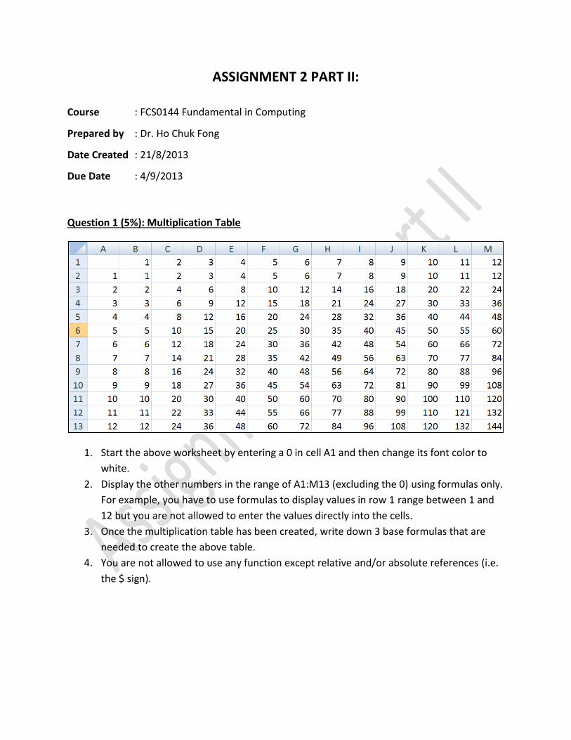
Question 1 (5%): Multiplication Table
1. Start the above worksheet by entering a 0 in cell A1 and then change its font color to
white.
2. Display the other numbers in the range of A1:M13 (excluding the 0) using formulas only.
For example, you have to use formulas to display values in row 1 range between 1 and
12 but you are not allowed to enter the values directly into the cells.
3. Once the multiplication table has been created, write down 3 base formulas that are
needed to create the above table.
4. You are not allowed to use any function except relative and/or absolute references (i.e.
the $ sign).
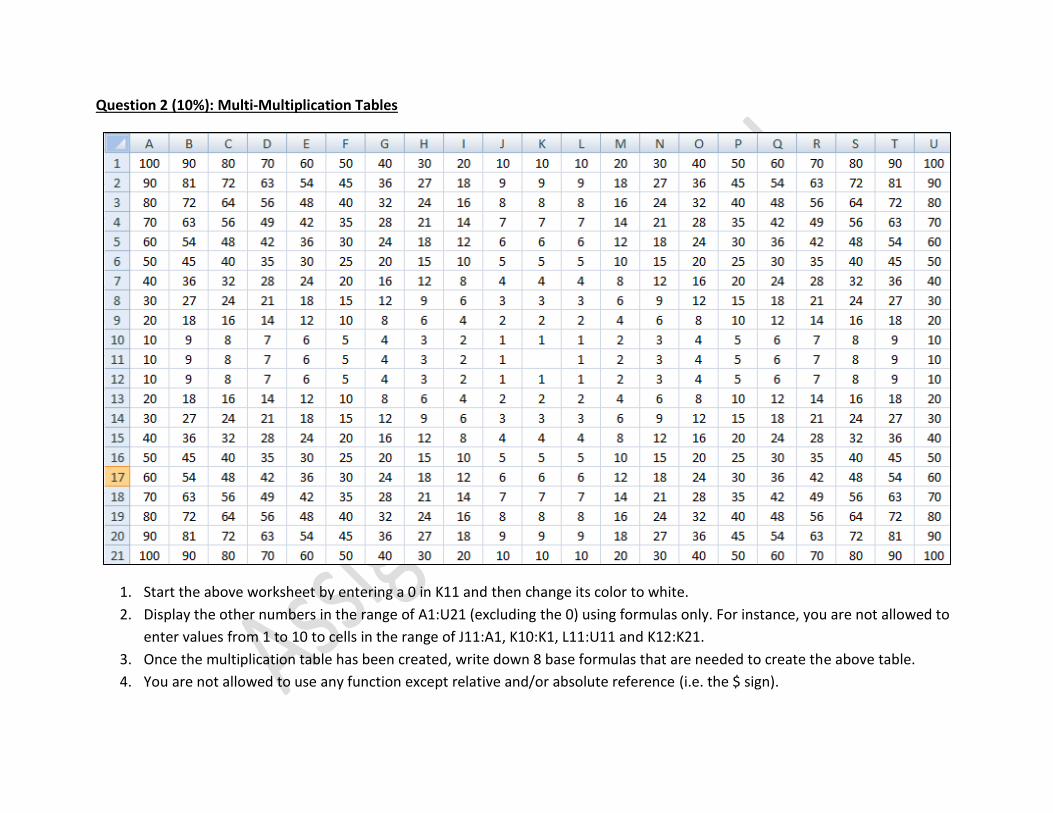
Question 2 (10%): Multi-Multiplication Tables
1. Start the above worksheet by entering a 0 in K11 and then change its color to white.
2. Display the other numbers in the range of A1:U21 (excluding the 0) using formulas only. For instance, you are not allowed to
enter values from 1 to 10 to cells in the range of J11:A1, K10:K1, L11:U11 and K12:K21.
3. Once the multiplication table has been created, write down 8 base formulas that are needed to create the above table.
4. You are not allowed to use any function except relative and/or absolute reference (i.e. the $ sign).
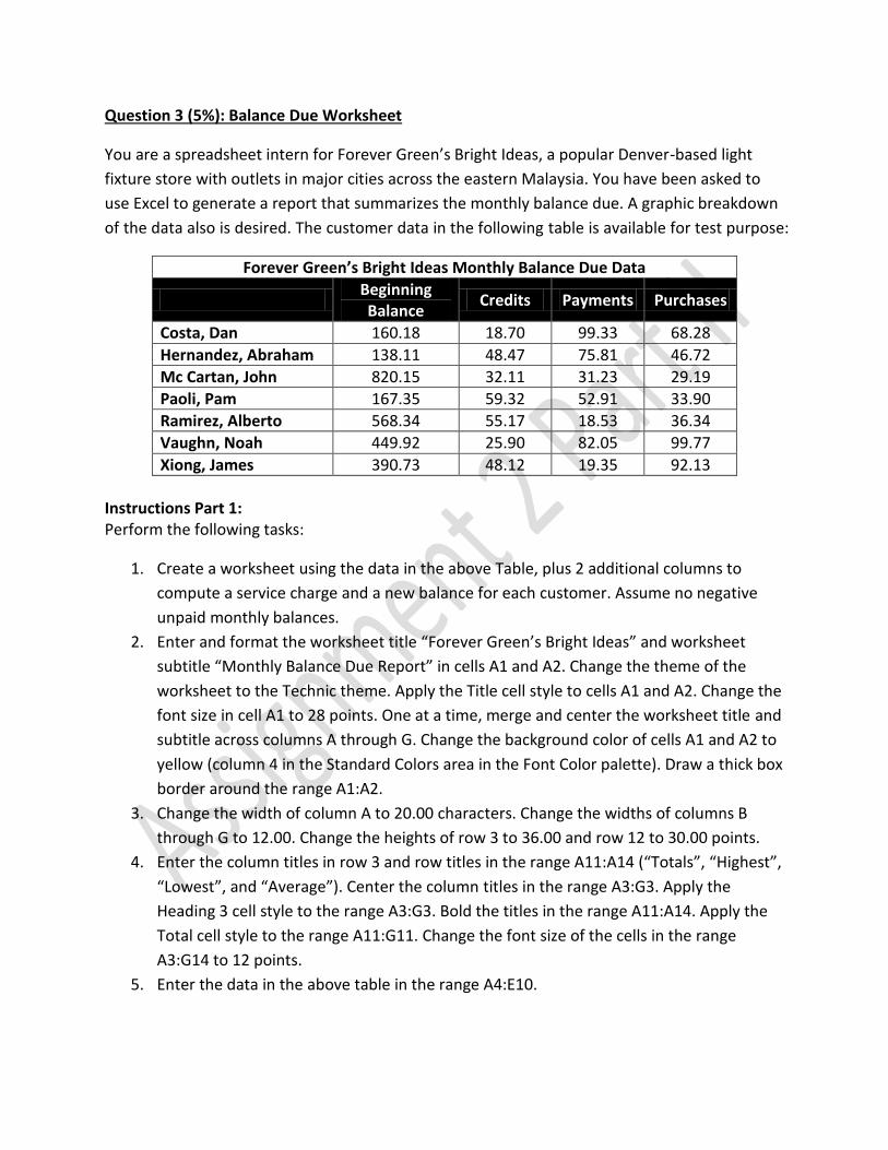
Question 3 (5%): Balance Due Worksheet
You are a spreadsheet intern for Forever Green’s Bright Ideas, a popular Denver-based light
fixture store with outlets in major cities across the eastern Malaysia. You have been asked to
use Excel to generate a report that summarizes the monthly balance due. A graphic breakdown
of the data also is desired. The customer data in the following table is available for test purpose:
Forever Green’s Bright Ideas Monthly Balance Due Data
Beginning Balance
Credits Payments Purchases
Costa, Dan 160.18 18.70 99.33 68.28
Hernandez, Abraham 138.11 48.47 75.81 46.72
Mc Cartan, John 820.15 32.11 31.23 29.19
Paoli, Pam 167.35 59.32 52.91 33.90
Ramirez, Alberto 568.34 55.17 18.53 36.34
Vaughn, Noah 449.92 25.90 82.05 99.77
Xiong, James 390.73 48.12 19.35 92.13
Instructions Part 1: Perform the following tasks:
1. Create a worksheet using the data in the above Table, plus 2 additional columns to
compute a service charge and a new balance for each customer. Assume no negative
unpaid monthly balances.
2. Enter and format the worksheet title “Forever Green’s Bright Ideas” and worksheet
subtitle “Monthly Balance Due Report” in cells A1 and A2. Change the theme of the
worksheet to the Technic theme. Apply the Title cell style to cells A1 and A2. Change the
font size in cell A1 to 28 points. One at a time, merge and center the worksheet title and
subtitle across columns A through G. Change the background color of cells A1 and A2 to
yellow (column 4 in the Standard Colors area in the Font Color palette). Draw a thick box
border around the range A1:A2.
3. Change the width of column A to 20.00 characters. Change the widths of columns B
through G to 12.00. Change the heights of row 3 to 36.00 and row 12 to 30.00 points.
4. Enter the column titles in row 3 and row titles in the range A11:A14 (“Totals”, “Highest”,
“Lowest”, and “Average”). Center the column titles in the range A3:G3. Apply the
Heading 3 cell style to the range A3:G3. Bold the titles in the range A11:A14. Apply the
Total cell style to the range A11:G11. Change the font size of the cells in the range
A3:G14 to 12 points.
5. Enter the data in the above table in the range A4:E10.
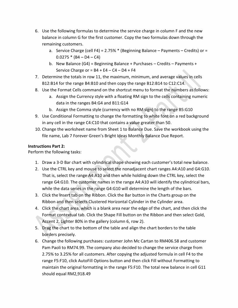
6. Use the following formulas to determine the service charge in column F and the new
balance in column G for the first customer. Copy the two formulas down through the
remaining customers.
a. Service Charge (cell F4) = 2.75% * (Beginning Balance – Payments – Credits) or =
0.0275 * (B4 – D4 – C4)
b. New Balance (G4) = Beginning Balance + Purchases – Credits – Payments +
Service Charge or = B4 + E4 – C4 – D4 + F4
7. Determine the totals in row 11, the maximum, minimum, and average values in cells
B12:B14 for the range B4:B10 and then copy the range B12:B14 to C12:C14.
8. Use the Format Cells command on the shortcut menu to format the numbers as follows:
a. Assign the Currency style with a floating RM sign to the cells containing numeric
data in the ranges B4:G4 and B11:G14
b. Assign the Comma style (currency with no RM sign) to the range B5:G10
9. Use Conditional Formatting to change the formatting to white font on a red background
in any cell in the range C4:C10 that contains a value greater than 50.
10. Change the worksheet name from Sheet 1 to Balance Due. Save the workbook using the
file name, Lab 7 Forever Green’s Bright Ideas Monthly Balance Due Report.
Instructions Part 2: Perform the following tasks:
1. Draw a 3-D Bar chart with cylindrical shape showing each customer’s total new balance.
2. Use the CTRL key and mouse to select the nonadjacent chart ranges A4:A10 and G4:G10.
That is, select the range A4:A10 and then while holding down the CTRL key, select the
range G4:G10. The customer names in the range A4:A10 will identify the cylindrical bars,
while the data series in the range G4:G10 will determine the length of the bars.
3. Click the Insert tab on the Ribbon. Click the Bar button in the Charts group on the
Ribbon and then selects Clustered Horizontal Cylinder in the Cylinder area.
4. Click the chart area, which is a blank area near the edge of the chart, and then click the
Format contextual tab. Click the Shape Fill button on the Ribbon and then select Gold,
Accent 2, Lighter 80% in the gallery (column 6, row 2).
5. Drag the chart to the bottom of the table and align the chart borders to the table
borders precisely.
6. Change the following purchases: customer John Mc Cartan to RM406.58 and customer
Pam Paoli to RM74.99. The company also decided to change the service charge from
2.75% to 3.25% for all customers. After copying the adjusted formula in cell F4 to the
range F5:F10, click AutoFill Options button and then click Fill without Formatting to
maintain the original formatting in the range F5:F10. The total new balance in cell G11
should equal RM2,918.49
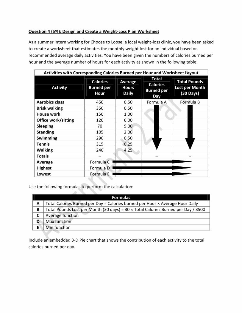
Question 4 (5%): Design and Create a Weight-Loss Plan Worksheet
As a summer intern working for Choose to Loose, a local weight-loss clinic, you have been asked
to create a worksheet that estimates the monthly weight lost for an individual based on
recommended average daily activities. You have been given the numbers of calories burned per
hour and the average number of hours for each activity as shown in the following table:
Activities with Corresponding Calories Burned per Hour and Worksheet Layout
Activity Calories
Burned per Hour
Average Hours Daily
Total Calories
Burned per Day
Total Pounds Lost per Month
(30 Days)
Aerobics class 450 0.50 Formula A Formula B
Brisk walking 350 0.50
House work 150 1.00
Office work/sitting 120 6.00
Sleeping 70 9.00
Standing 105 2.00
Swimming 290 0.50
Tennis 315 0.25
Walking 240 4.25
Totals – – –
Average Formula C
Highest Formula D
Lowest Formula E
Use the following formulas to perform the calculation:
Formulas
A Total Calories Burned per Day = Calories burned per Hour × Average Hour Daily
B Total Pounds Lost per Month (30 days) = 30 × Total Calories Burned per Day / 3500
C Average function
D Max function
E Min function
Include an embedded 3-D Pie chart that shows the contribution of each activity to the total
calories burned per day.
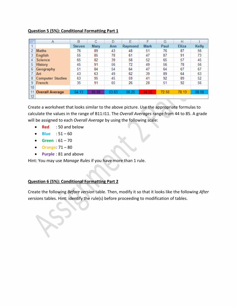
Question 5 (5%): Conditional Formatting Part 1
Create a worksheet that looks similar to the above picture. Use the appropriate formulas to
calculate the values in the range of B11:I11. The Overall Averages range from 44 to 85. A grade
will be assigned to each Overall Average by using the following scale:
Red : 50 and below
Blue : 51 – 60
Green : 61 – 70
Orange: 71 – 80
Purple : 81 and above
Hint: You may use Manage Rules if you have more than 1 rule.
Question 6 (5%): Conditional Formatting Part 2
Create the following Before version table. Then, modify it so that it looks like the following After
versions tables. Hint: identify the rule(s) before proceeding to modification of tables.
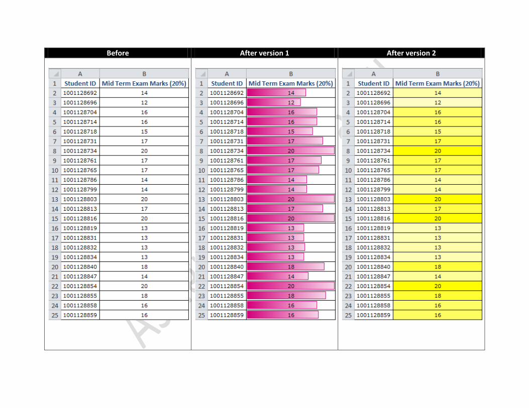
Before After version 1 After version 2
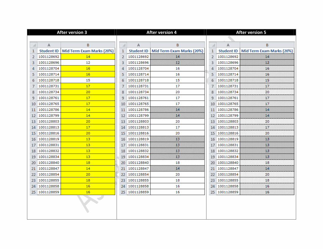
After version 3 After version 4 After version 5
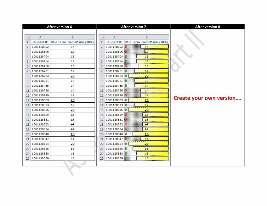
After version 6 After version 7 After version 8
Create your own version….
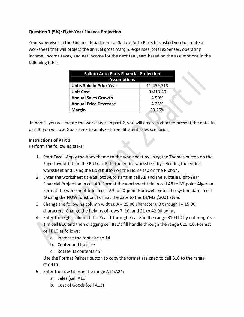
Question 7 (5%): Eight-Year Finance Projection
Your supervisor in the Finance department at Salioto Auto Parts has asked you to create a
worksheet that will project the annual gross margin, expenses, total expenses, operating
income, income taxes, and net income for the next ten years based on the assumptions in the
following table.
Salioto Auto Parts Financial Projection Assumptions
Units Sold in Prior Year 11,459,713
Unit Cost RM13.40
Annual Sales Growth 4.50%
Annual Price Decrease 4.25%
Margin 39.25%
In part 1, you will create the worksheet. In part 2, you will create a chart to present the data. In
part 3, you will use Goals Seek to analyze three different sales scenarios.
Instructions of Part 1: Perform the following tasks:
1. Start Excel. Apply the Apex theme to the worksheet by using the Themes button on the
Page Layout tab on the Ribbon. Bold the entire worksheet by selecting the entire
worksheet and using the Bold button on the Home tab on the Ribbon.
2. Enter the worksheet title Salioto Auto Parts in cell A8 and the subtitle Eight-Year
Financial Projection in cell A9. Format the worksheet title in cell A8 to 36-point Algerian.
Format the worksheet title in cell A9 to 20-point Rockwell. Enter the system date in cell
I9 using the NOW function. Format the date to the 14/Mar/2001 style.
3. Change the following column widths: A = 25.00 characters; B through I = 15.00
characters. Change the heights of rows 7, 10, and 21 to 42.00 points.
4. Enter the eight column titles Year 1 through Year 8 in the range B10:I10 by entering Year
1 in cell B10 and then dragging cell B10’s fill handle through the range C10:I10. Format
cell B10 as follows:
a. Increase the font size to 14
b. Center and Italicize
c. Rotate its contents 45°
Use the Format Painter button to copy the format assigned to cell B10 to the range
C10:I10.
5. Enter the row titles in the range A11:A24:
a. Sales (cell A11)
b. Cost of Goods (cell A12)
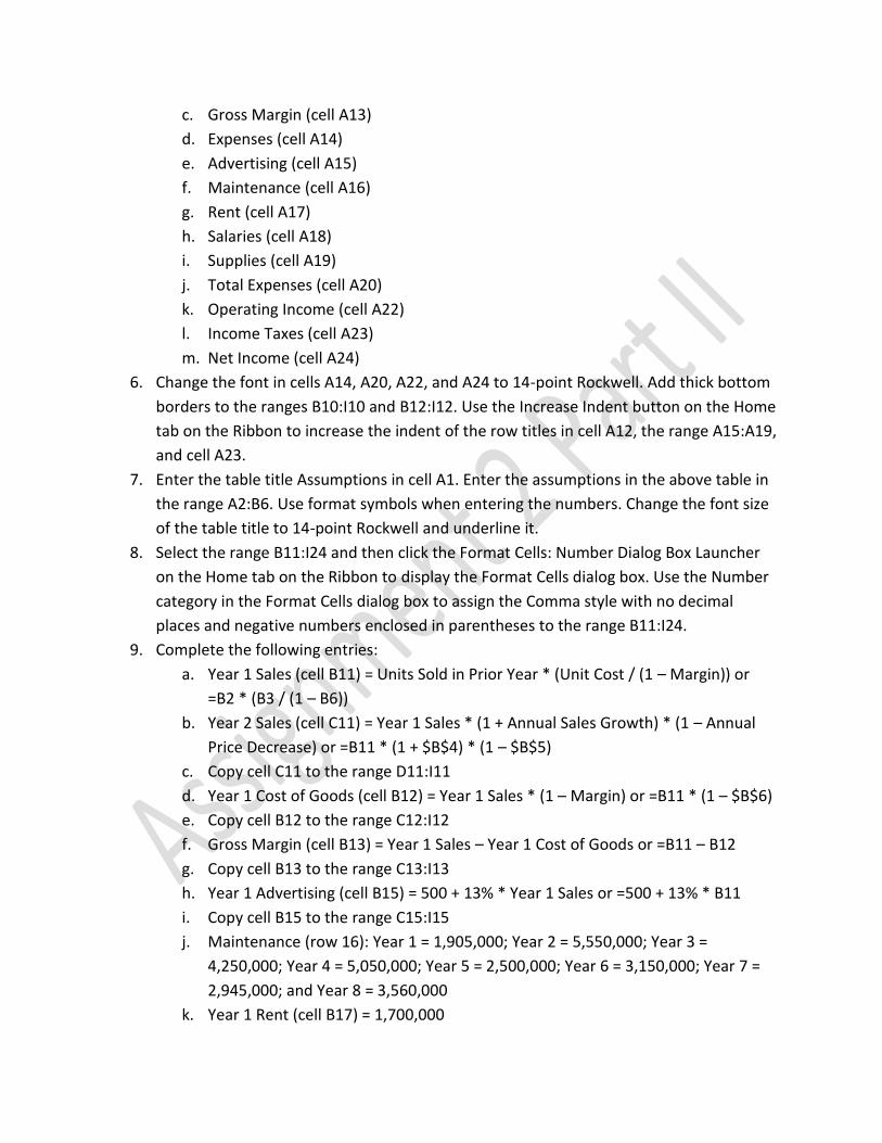
c. Gross Margin (cell A13)
d. Expenses (cell A14)
e. Advertising (cell A15)
f. Maintenance (cell A16)
g. Rent (cell A17)
h. Salaries (cell A18)
i. Supplies (cell A19)
j. Total Expenses (cell A20)
k. Operating Income (cell A22)
l. Income Taxes (cell A23)
m. Net Income (cell A24)
6. Change the font in cells A14, A20, A22, and A24 to 14-point Rockwell. Add thick bottom
borders to the ranges B10:I10 and B12:I12. Use the Increase Indent button on the Home
tab on the Ribbon to increase the indent of the row titles in cell A12, the range A15:A19,
and cell A23.
7. Enter the table title Assumptions in cell A1. Enter the assumptions in the above table in
the range A2:B6. Use format symbols when entering the numbers. Change the font size
of the table title to 14-point Rockwell and underline it.
8. Select the range B11:I24 and then click the Format Cells: Number Dialog Box Launcher
on the Home tab on the Ribbon to display the Format Cells dialog box. Use the Number
category in the Format Cells dialog box to assign the Comma style with no decimal
places and negative numbers enclosed in parentheses to the range B11:I24.
9. Complete the following entries:
a. Year 1 Sales (cell B11) = Units Sold in Prior Year * (Unit Cost / (1 – Margin)) or
=B2 * (B3 / (1 – B6))
b. Year 2 Sales (cell C11) = Year 1 Sales * (1 + Annual Sales Growth) * (1 – Annual
Price Decrease) or =B11 * (1 + $B$4) * (1 – $B$5)
c. Copy cell C11 to the range D11:I11
d. Year 1 Cost of Goods (cell B12) = Year 1 Sales * (1 – Margin) or =B11 * (1 – $B$6)
e. Copy cell B12 to the range C12:I12
f. Gross Margin (cell B13) = Year 1 Sales – Year 1 Cost of Goods or =B11 – B12
g. Copy cell B13 to the range C13:I13
h. Year 1 Advertising (cell B15) = 500 + 13% * Year 1 Sales or =500 + 13% * B11
i. Copy cell B15 to the range C15:I15
j. Maintenance (row 16): Year 1 = 1,905,000; Year 2 = 5,550,000; Year 3 =
4,250,000; Year 4 = 5,050,000; Year 5 = 2,500,000; Year 6 = 3,150,000; Year 7 =
2,945,000; and Year 8 = 3,560,000
k. Year 1 Rent (cell B17) = 1,700,000
l. Year 2 Rent (cell C17) = Year 1 Rent + (10% * Year 1 Rent) or =B17 * (1 + 10%)
m. Copy cell C17 to the range D17:I17
n. Year 1 Salaries (cell B18) = 22.25% * Year 1 Sales or =22.25% * B11
o. Copy cell B18 to the range C18:I18
p. Year 1 Supplies (cell B19) = 1.5% * Year 1 Sales or =1.5% * B11
q. Copy cell B19 to the range C19:I19
r. Year 1 Total Expenses (cell B20) or =SUM(B15:B19)
s. Copy cell B20 to the range C20:I20
t. Year 1 Operating Income (cell B22) = Year 1 Gross Margin – Year 1 Total Expenses
or =B13 – B20
u. Copy cell B22 to the range C22:I22
v. Year 1 Income Taxes (cell B23): If Year 1 Operating Income is less than 0, then
Year 1 Income Taxes equal 0, otherwise Year 1 Income Taxes equal 40% * Year 1
Operating Income or =IF(B22 < 0, 0, 40% * B22)
w. Copy cell B23 to the range C23:I23
x. Year 1 Net Income (cell B24) = Year 1 Operating Income – Year 1 Income Taxes or
=B22 – B23
y. Copy cell B24 to the range C24:I24
10. Use Orange (column 3 under Standard Colors) for the background colors of A1:B6, A8:I9,
A14, A20, A22:I22, and A24:I24.
11. Save the workbook.
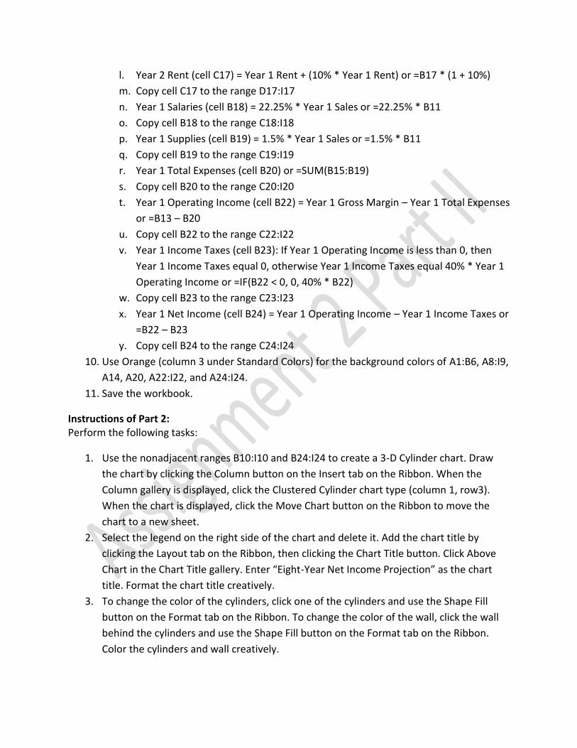
Instructions of Part 2: Perform the following tasks:
1. Use the nonadjacent ranges B10:I10 and B24:I24 to create a 3-D Cylinder chart. Draw
the chart by clicking the Column button on the Insert tab on the Ribbon. When the
Column gallery is displayed, click the Clustered Cylinder chart type (column 1, row3).
When the chart is displayed, click the Move Chart button on the Ribbon to move the
chart to a new sheet.
2. Select the legend on the right side of the chart and delete it. Add the chart title by
clicking the Layout tab on the Ribbon, then clicking the Chart Title button. Click Above
Chart in the Chart Title gallery. Enter “Eight-Year Net Income Projection” as the chart
title. Format the chart title creatively.
3. To change the color of the cylinders, click one of the cylinders and use the Shape Fill
button on the Format tab on the Ribbon. To change the color of the wall, click the wall
behind the cylinders and use the Shape Fill button on the Format tab on the Ribbon.
Color the cylinders and wall creatively.
4. Rename the sheet tabs as “Eight-Year Financial Projection” and “3-D Cylinder Chart”.
Color their tabs as well.
5. Save the workbook.
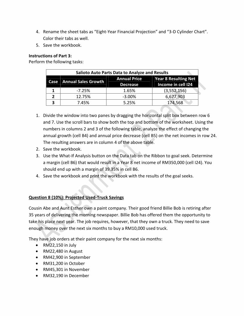
Instructions of Part 3: Perform the following tasks:
Salioto Auto Parts Data to Analyze and Results
Case Annual Sales Growth Annual Price
Decrease Year 8 Resulting Net
Income in cell I24
1 -7.25% 1.65% (3,552,156)
2 12.75% -3.00% 6,677,903
3 7.45% 5.25% 174,568
1. Divide the window into two panes by dragging the horizontal split box between row 6
and 7. Use the scroll bars to show both the top and bottom of the worksheet. Using the
numbers in columns 2 and 3 of the following table, analyze the effect of changing the
annual growth (cell B4) and annual price decrease (cell B5) on the net incomes in row 24.
The resulting answers are in column 4 of the above table.
2. Save the workbook.
3. Use the What-If Analysis button on the Data tab on the Ribbon to goal seek. Determine
a margin (cell B6) that would result in a Year 8 net income of RM350,000 (cell I24). You
should end up with a margin of 39.35% in cell B6.
4. Save the workbook and print the workbook with the results of the goal seeks.
Question 8 (10%): Projected Used-Truck Savings
Cousin Abe and Aunt Esther own a paint company. Their good friend Billie Bob is retiring after
35 years of delivering the morning newspaper. Billie Bob has offered them the opportunity to
take his place next year. The job requires, however, that they own a truck. They need to save
enough money over the next six months to buy a RM10,000 used truck.
They have job orders at their paint company for the next six months:
RM22,150 in July
RM22,480 in August
RM42,900 in September
RM31,200 in October
RM45,301 in November
RM32,190 in December
Each month, they spend parts of the job order income for the following expenses:
34.55% on material
3.00% on rollers and brushes
4.75% on their retirement account
39.50% on food and clothing
25% of the remaining profits (orders – total expenses) will be put aside for the used truck
Aunt Esther’s retired parents have agreed to provide a bonus of RM250 whenever the monthly
savings for the truck exceeds RM2,000. Use the concepts and techniques presented in this
project to create and format the worksheet.
Cousin Abe has asked you to create a worksheet that shows orders, expenses, profits, bonuses,
and savings for the next six months, and totals for each category. Aunt Esther would like to save
for another used truck for RM17,000. She has asked you to:
1. Perform a What-If analysis to determine the effect on the savings by reducing the
percentage spent on material to 22% (answer total savings ≈ RM16,084.49)
2. With the original assumptions, goal seek to determine what percentage of profits to
spend on food and clothing if RM15,000 is needed for the used truck (answer ≈ 29.16%)
Print the workbook with the results of the What-If analysis.
Note:
1. You must submit your assignment in both hard-copy (face-to-face in the classroom) and
soft-copy (via mystudy.unimy.edu.my) forms.
2. Any assignments submitted after due date or involving plagiarism will be marked, but
given zero mark.
3. Any information taken from the work of others should be acknowledged by reference to
obviate the charge of copying.
4. Color printing is not required, black and white printing is sufficient.
Recommended