Math6911, S08, HM Zhu
7.1 Stop and loss hedging
7. Greek Letters, Value-at-Risk
(Hull’s book, Chapter 15)
2Math6911, S08, HM ZHU
Outline (Hull, Chap 15.1-15.3; Brandimarte, Chap 8.1.2)
• Naked and cover position• Stop-Loss Strategy• Simulating the stop-loss strategy
3Math6911, S08, HM ZHU
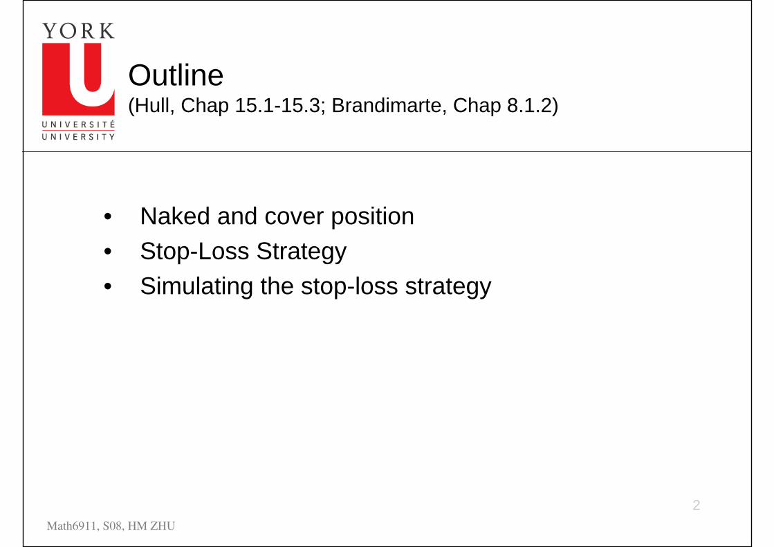
Example
• A bank has sold for $7.00 a European call option on one share of a nondividend paying stockS0 = $50, K = $50, r = 5%, σ = 40%,
T = 5 months, µ = 10%• The Black-Scholes value of the option is $5.6150• How does the bank hedge its risk?
4Math6911, S08, HM ZHU
Naked & Covered Positions
• Naked position: Take no action
• Covered position: Buy 1 share today
• Either strategy leaves the bank exposed to significant risk
5Math6911, S08, HM ZHU
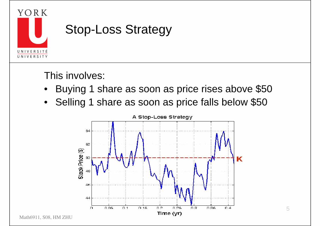
Stop-Loss Strategy
This involves:• Buying 1 share as soon as price rises above $50• Selling 1 share as soon as price falls below $50
6Math6911, S08, HM ZHU
Stop-Loss Strategy
• This simple hedging strategy is to ensure that at time T, the bank owns the stock if the option closes in the money and dose not own it if the option closes out of money
• We can evaluate its performance in discrete time by Monte Carlo simulation
7Math6911, S08, HM ZHU
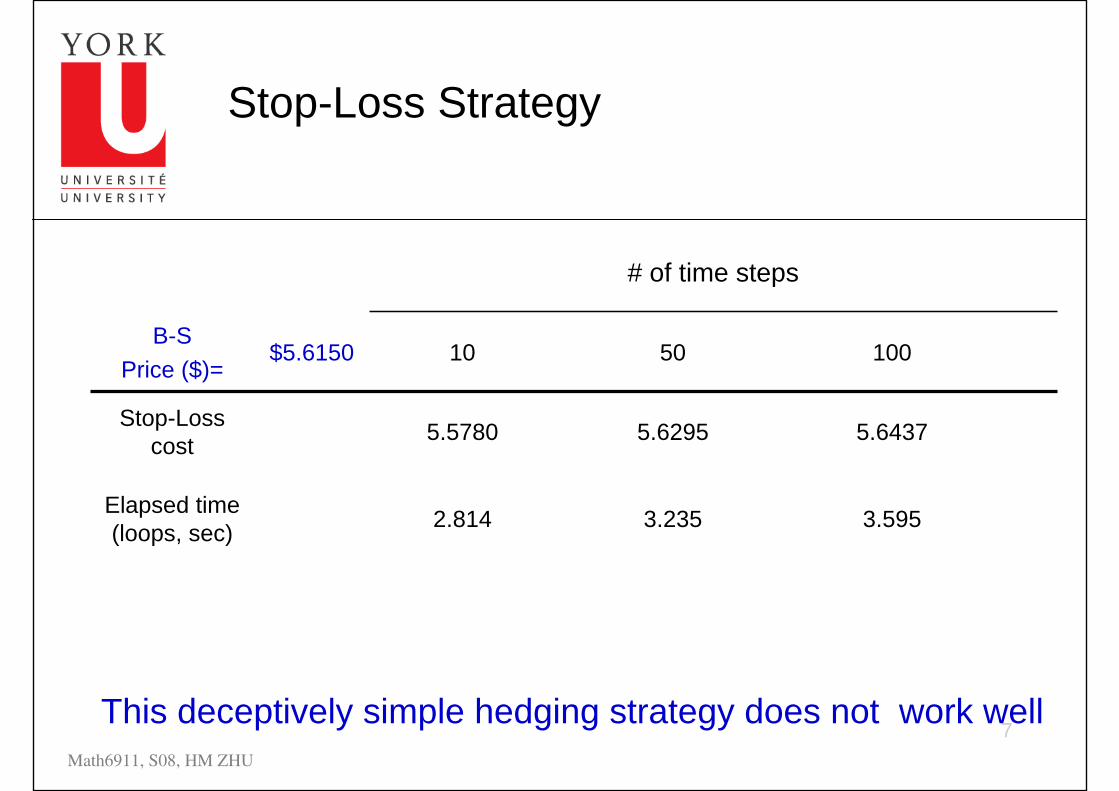
3.5953.2352.814 Elapsed time (loops, sec)
5.64375.62955.5780Stop-Loss cost
1005010$5.6150B-S
Price ($)=
# of time steps
Stop-Loss Strategy
This deceptively simple hedging strategy does not work well
Math6911, S08, HM Zhu
7.2 Greek Letters
7. Greek Letters, Value-at-Risk
(Hull’s book, Chapter 15)
9Math6911, S08, HM ZHU
Outline
• Delta, Delta hedging• Theta • Gamma• Relationship between delta, Theta and Gamma• Vega
10Math6911, S08, HM ZHU
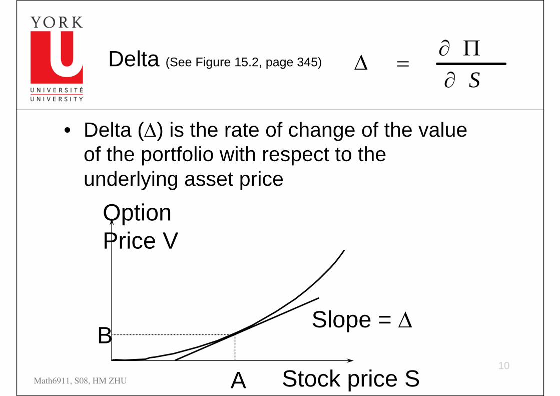
Delta (See Figure 15.2, page 345)
• Delta (∆) is the rate of change of the value of the portfolio with respect to the underlying asset price
OptionPrice V
A
BSlope = ∆
Stock price S
S∂ Π
∆ =∂
11Math6911, S08, HM ZHU
Delta
• An important parameter in the pricing and hedging of options
• It is # of the units of the stock we should hold for each option shorted to create a riskless hedge. Such a construction of riskless hedging is called “delta hedging”.
• ∆ of a call option is positive whereas ∆ of a put option is negative
12Math6911, S08, HM ZHU
Delta Hedging
• This involves maintaining a delta neutral portfolio• The hedge position must be frequently rebalanced• Delta hedging a written option involves a “buy high,
sell low” trading rule
13Math6911, S08, HM ZHU
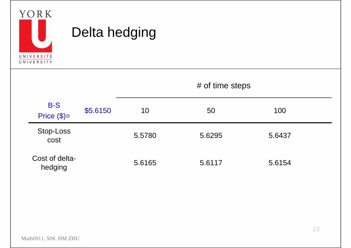
5.61545.61175.6165 Cost of delta-hedging
5.64375.62955.5780Stop-Loss cost
1005010$5.6150B-S
Price ($)=
# of time steps
Delta hedging
14Math6911, S08, HM ZHU
Theta
• Theta (Θ) of a derivative (or portfolio of derivatives) is the rate of change of the value with respect to the passage of time
• The theta of a call or put is usually negative. This means that, if time passes with the price of the underlying asset and its volatility remaining the same, the value of the option declines
t∂Π
Θ =∂
15Math6911, S08, HM ZHU
Gamma
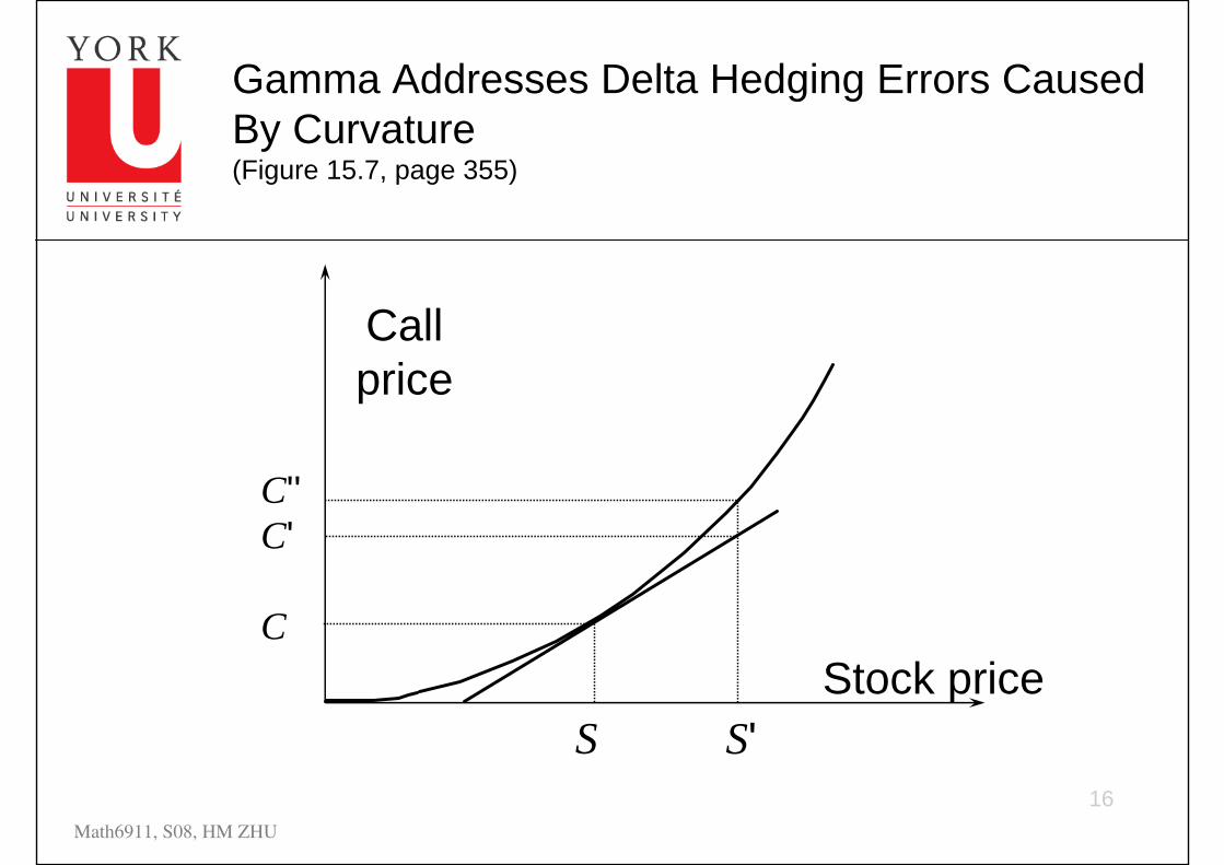
• Gamma (Γ) is the rate of change of delta (∆) with respect to the price of the underlying asset
• Gamma neutrality protects against large change in the price of the underlying asset between hedge re-balancing
2
2S∂ Π
Γ =∂
16Math6911, S08, HM ZHU
Gamma Addresses Delta Hedging Errors Caused By Curvature (Figure 15.7, page 355)
S
CStock price
S'
Callprice
C''C'
17Math6911, S08, HM ZHU
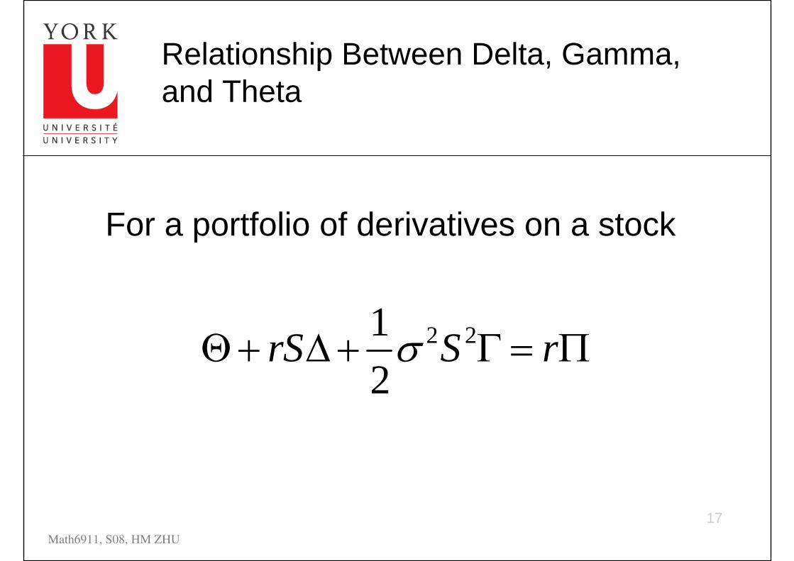
Relationship Between Delta, Gamma, and Theta
For a portfolio of derivatives on a stock
2 212
rS S rσΘ + ∆ + Γ = Π
18Math6911, S08, HM ZHU
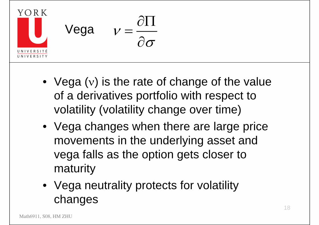
Vega
• Vega (ν) is the rate of change of the value of a derivatives portfolio with respect to volatility (volatility change over time)
• Vega changes when there are large price movements in the underlying asset and vega falls as the option gets closer to maturity
• Vega neutrality protects for volatility changes
νσ
∂Π=
∂
19Math6911, S08, HM ZHU
Hedging in Practice
• Traders usually ensure that their portfolios are delta-neutral at least once a day
• Traders monitor gamma and vega. If they get too large, either corrective action is taken or trading is curtailed.
Math6911, S08, HM Zhu
7. Greek Letters, Value-at-Risk
7.3 Value-at-Risk
(Hull’s, Chapter 18)
21Math6911, S08, HM ZHU
Outline (Hull, Chap 18)
• What is Value at Risk (VaR)? • Historical simulations• Monte Carlo simulations • Model based approach
–Variance-covariance method• Comparisons of methods• Testing
22Math6911, S08, HM ZHU
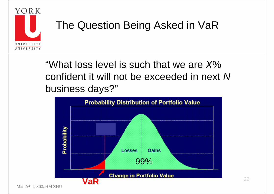
The Question Being Asked in VaR
“What loss level is such that we are X% confident it will not be exceeded in next Nbusiness days?”
VaR
99%
23Math6911, S08, HM ZHU
VaR and Regulatory Capital(Hull’s Business Snapshot 18.1, page 436)
• We are X% certain that we will not lose more than V dollars in the next N days
• VaR is the loss level V that will not be exceeded with a specified probability
• Regulators use VaR in determining the capital a bank is required to to keep to reflect the market risks it is bearing
• The market-risk capital is k times the 10-day 99% VaR where k is at least 3.0
24Math6911, S08, HM ZHU
Advantages of VaR
• It captures an important aspect of risk in a single number
• It is easy to understand• It asks the simple question: “How bad can
things get?”
25Math6911, S08, HM ZHU
Time Horizon N
• Instead of calculating the N-day, X% VaR directly analysts usually calculate a 1-day X% VaR and assume
• This is exactly true when portfolio changes on successive days come from independent identically distributed normal distributions
N-day VaR 1-day VaRN= ×
26Math6911, S08, HM ZHU
Methods of Estimating VaR
• Historical simulations• Monte Carlo simulations• Model building approaches
27Math6911, S08, HM ZHU
Historical Simulation (Hull, See Tables 18.1 and 18.2, page 438-439))
• Create a database of the daily movements in all market variables.
• The first simulation trial assumes that the percentage changes in all market variables are as on the first day
• The second simulation trial assumes that the percentage changes in all market variables are as on the second day
• and so on
28Math6911, S08, HM ZHU
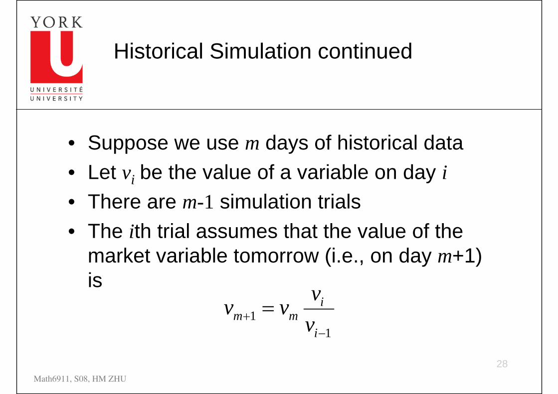
Historical Simulation continued
• Suppose we use m days of historical data• Let vi be the value of a variable on day i• There are m-1 simulation trials• The ith trial assumes that the value of the
market variable tomorrow (i.e., on day m+1) is
11
im m
i
vv vv+
−
=
29Math6911, S08, HM ZHU
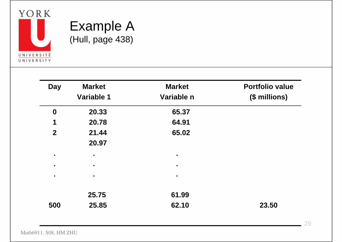
Example A (Hull, page 438)
012
.
.
.
500
Day
23.50
65.3764.9165.02
.
.
.
61.9962.10
20.3320.7821.4420.97...
25.7525.85
Portfolio value($ millions)
MarketVariable n
MarketVariable 1
30Math6911, S08, HM ZHU
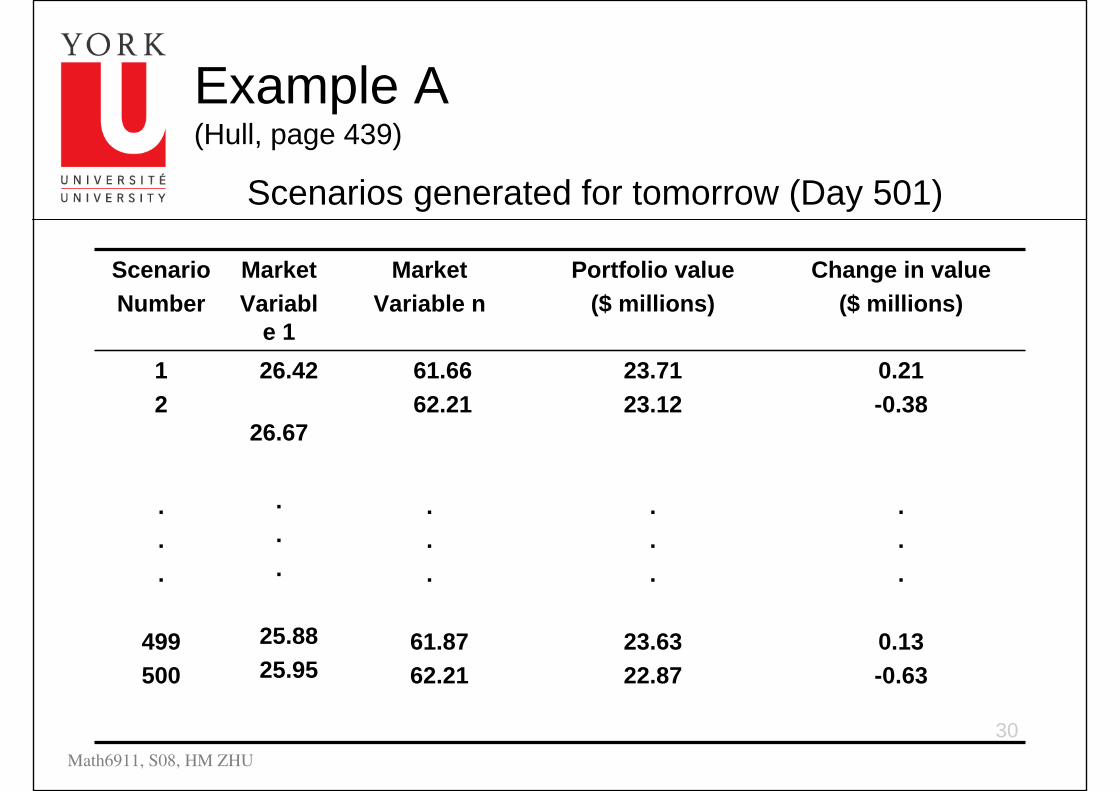
Example A (Hull, page 439)
0.21-0.38
.
.
.
0.13-0.63
Change in value($ millions)
12
.
.
.
499500
ScenarioNumber
23.7123.12
.
.
.
23.6322.87
61.6662.21
.
.
.
61.8762.21
26.42
26.67
.
.
.
25.8825.95
Portfolio value($ millions)
MarketVariable n
MarketVariabl
e 1
Scenarios generated for tomorrow (Day 501)

31Math6911, S08, HM ZHU
Example B
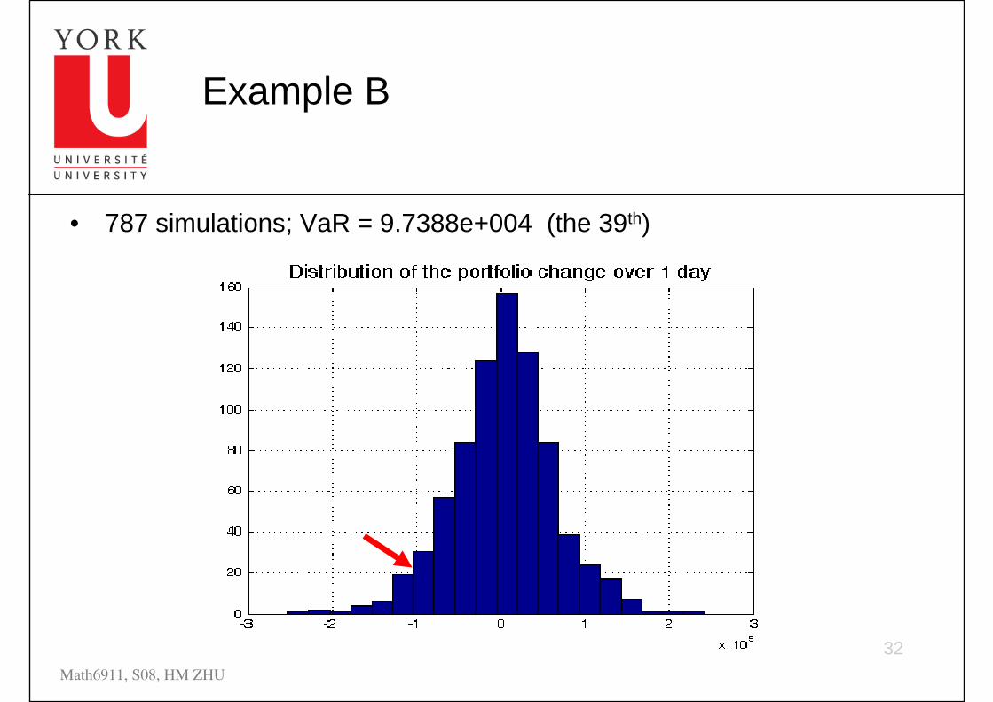
• A portfolio consist of 9 different stocks• The number of each stock in the portfolio is
905 569 632 234 549 932 335 656 392, respectively.
• We have 3 year historical data of each stock
• Estimate 1-Day 95% VaR using historical simulations
32Math6911, S08, HM ZHU
Example B
• 787 simulations; VaR = 9.7388e+004 (the 39th)
33Math6911, S08, HM ZHU
Monte Carlo Simulation (page 448-449)
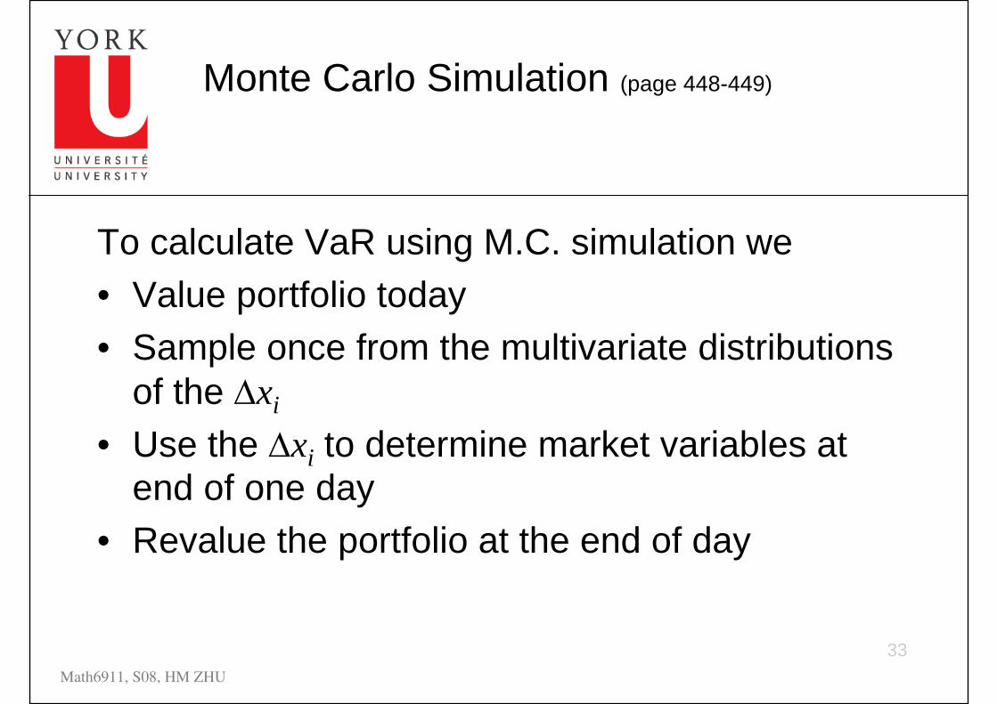
To calculate VaR using M.C. simulation we• Value portfolio today• Sample once from the multivariate distributions
of the ∆xi
• Use the ∆xi to determine market variables at end of one day
• Revalue the portfolio at the end of day
34Math6911, S08, HM ZHU
Monte Carlo Simulation
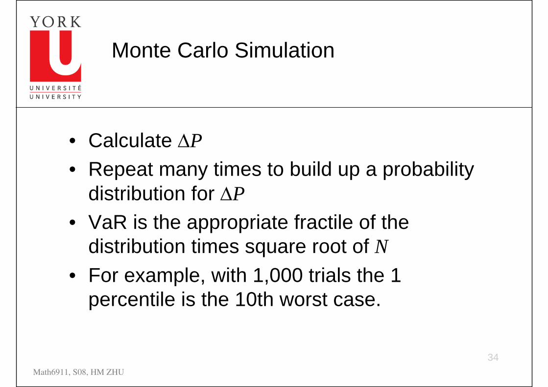
• Calculate ∆P• Repeat many times to build up a probability
distribution for ∆P• VaR is the appropriate fractile of the
distribution times square root of N• For example, with 1,000 trials the 1
percentile is the 10th worst case.
35Math6911, S08, HM ZHU
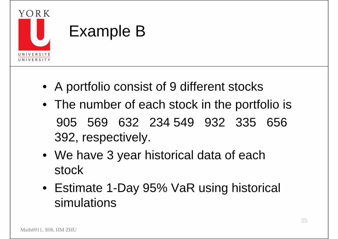
Example B
• A portfolio consist of 9 different stocks• The number of each stock in the portfolio is
905 569 632 234 549 932 335 656 392, respectively.
• We have 3 year historical data of each stock
• Estimate 1-Day 95% VaR using historical simulations
36Math6911, S08, HM ZHU
Example B
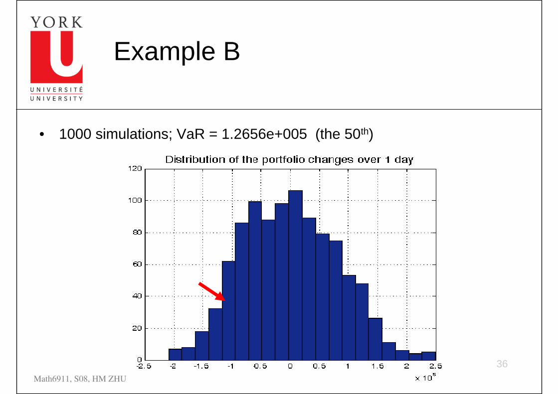
• 1000 simulations; VaR = 1.2656e+005 (the 50th)
37Math6911, S08, HM ZHU
The Model-Building Approach
• Another alternative approach is to make assumptions about the probability distributions of return on the market variables and calculate the probability distribution of the change in the value of the portfolio analytically
• This is known as the model building approach or the variance-covariance approach
38Math6911, S08, HM ZHU
Daily Volatilities
• In option pricing we measure volatility “per year”
• In VaR calculations we measure volatility “per day”
6252year
day year%σ
σ σ= ≈
39Math6911, S08, HM ZHU
Daily Volatility continued
• Strictly speaking we should define σday as the standard deviation of the continuously compounded return in one day
• In practice we assume that it is the standard deviation of the percentage change in one day
40Math6911, S08, HM ZHU
Microsoft Example (page 440)
• We have a position worth $10 million in Microsoft shares
• The volatility of Microsoft is 2% per day (about 32% per year)
• We use N=10 and X=99
41Math6911, S08, HM ZHU
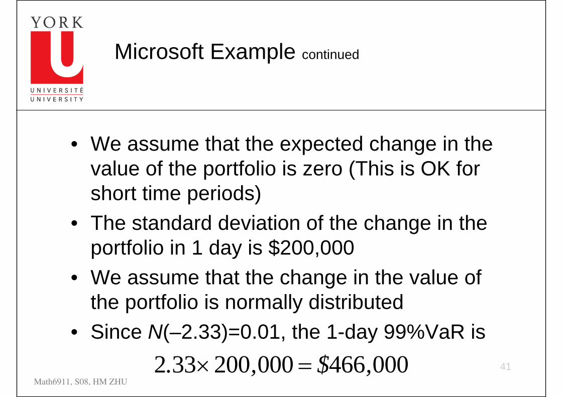
Microsoft Example continued
• We assume that the expected change in the value of the portfolio is zero (This is OK for short time periods)
• The standard deviation of the change in the portfolio in 1 day is $200,000
• We assume that the change in the value of the portfolio is normally distributed
• Since N(–2.33)=0.01, the 1-day 99%VaR is 2 33 200 000 466 000. , $ ,× =
42Math6911, S08, HM ZHU
Microsoft Example continued
• The 10-day 99% VaR
466 000 10 1 473 621, $ , ,=
43Math6911, S08, HM ZHU
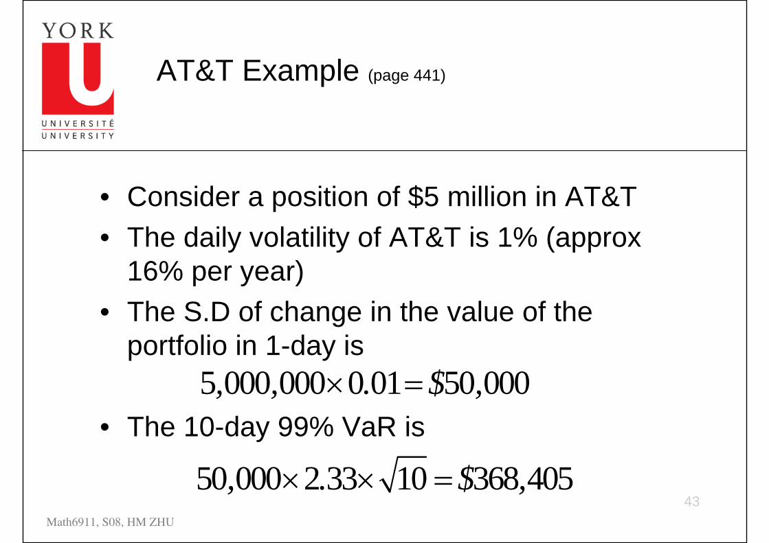
AT&T Example (page 441)
• Consider a position of $5 million in AT&T• The daily volatility of AT&T is 1% (approx
16% per year)• The S.D of change in the value of the
portfolio in 1-day is
• The 10-day 99% VaR is5 000 000 0 01 50 000, , . $ ,× =
50 000 2 33 10 368 405, . $ ,× × =
44Math6911, S08, HM ZHU
Portfolio
• Now consider a portfolio consisting of both Microsoft and AT&T
• Suppose that the correlation between the returns is 0.3
• X: change in the value of the position in Microsoft over 1-day period
• Y: change in the value of the position in AT&T over 1-day period
45Math6911, S08, HM ZHU
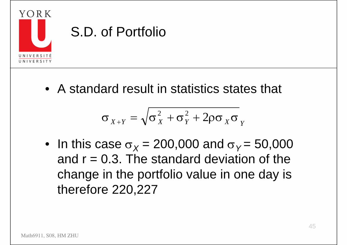
S.D. of Portfolio
• A standard result in statistics states that
• In this case σX = 200,000 and σY = 50,000 and r = 0.3. The standard deviation of the change in the portfolio value in one day is therefore 220,227
YXYXYX σρσ+σ+σ=σ + 222
46Math6911, S08, HM ZHU
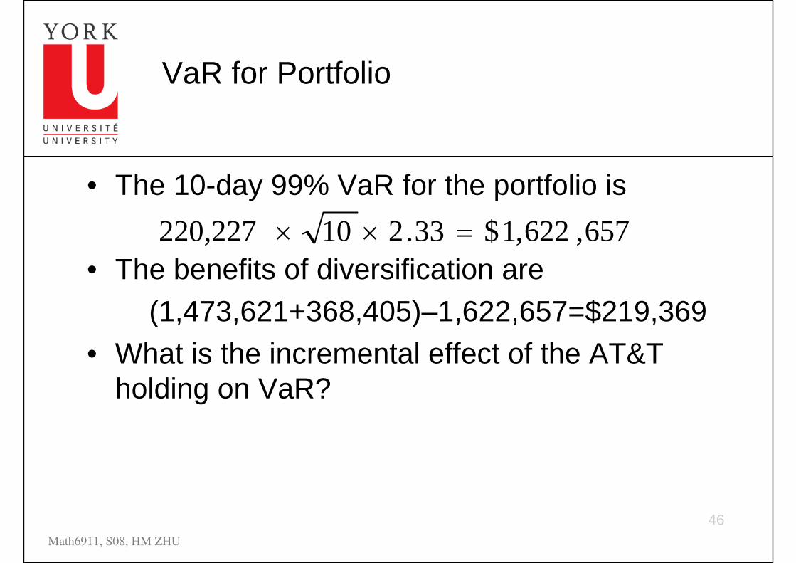
VaR for Portfolio
• The 10-day 99% VaR for the portfolio is
• The benefits of diversification are(1,473,621+368,405)–1,622,657=$219,369
• What is the incremental effect of the AT&T holding on VaR?
657,622,1$33.210220,227 =××
47Math6911, S08, HM ZHU
The Linear Model
We assume• The daily change in the value of a portfolio
is linearly related to the daily returns from market variables
• The returns from the market variables are normally distributed
48Math6911, S08, HM ZHU
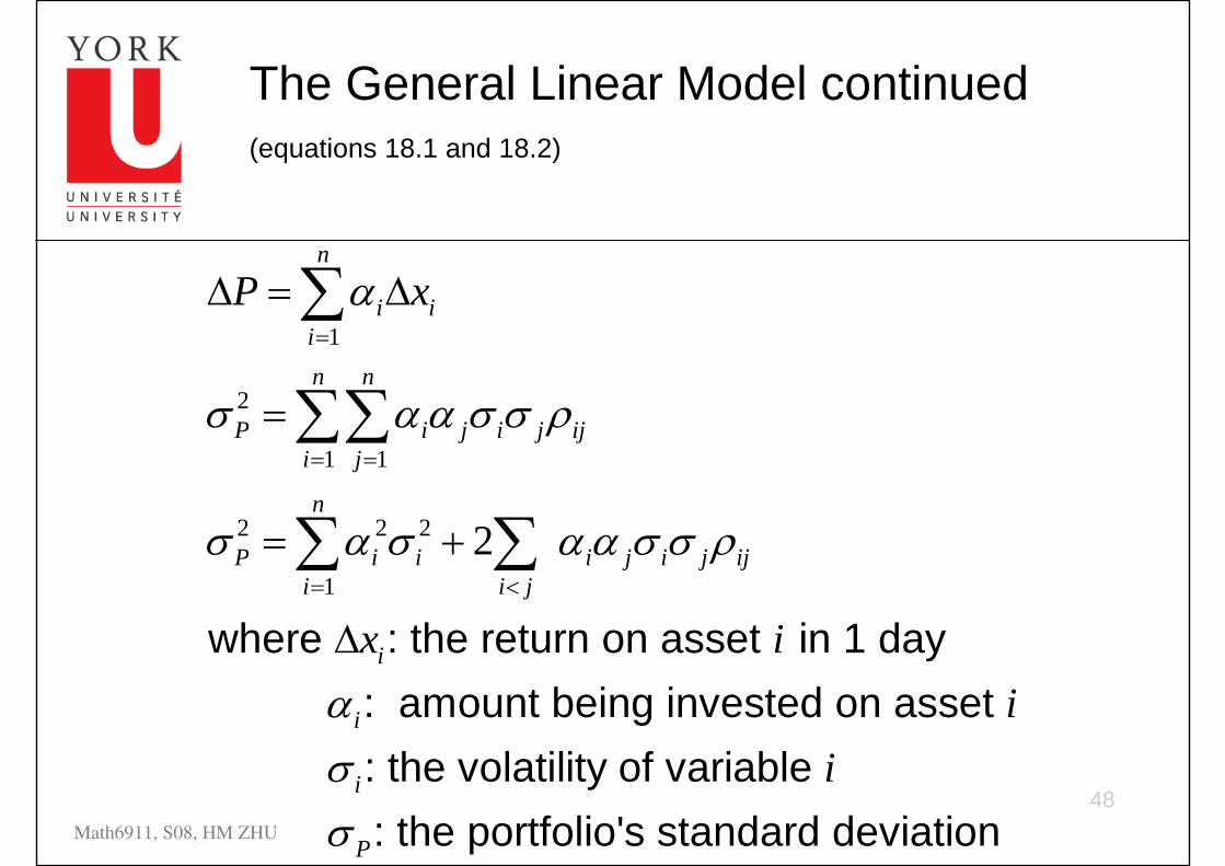
The General Linear Model continued (equations 18.1 and 18.2)
1
2
1 1
2 2 2
12
where : the return on asset in 1 day : amount being invested on asset : the volatility of variable
n
i iin n
P i j i j iji j
n
P i i i j i j iji i j
i
i
i
P x
x ii
i
α
σ α α σ σ ρ
σ α σ α α σ σ ρ
ασ
=
= =
= <
∆ = ∆
=
= +
∆
∑
∑∑
∑ ∑
: the portfolio's standard deviationPσ
49Math6911, S08, HM ZHU
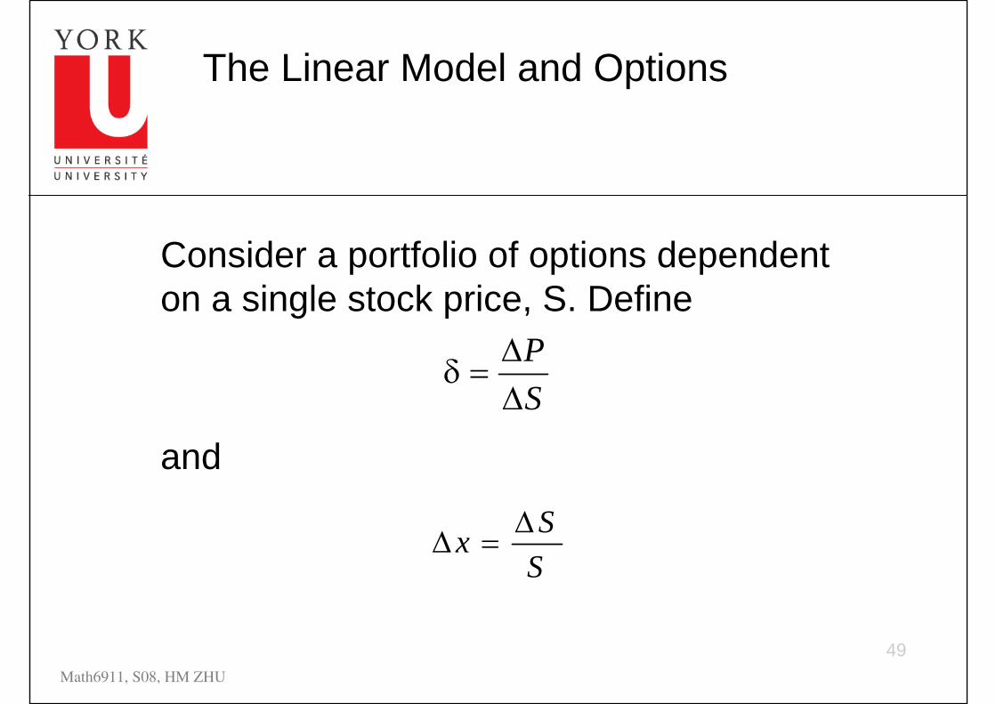
The Linear Model and Options
Consider a portfolio of options dependent on a single stock price, S. Define
andSP
∆∆
=δ
SSx ∆
=∆
50Math6911, S08, HM ZHU
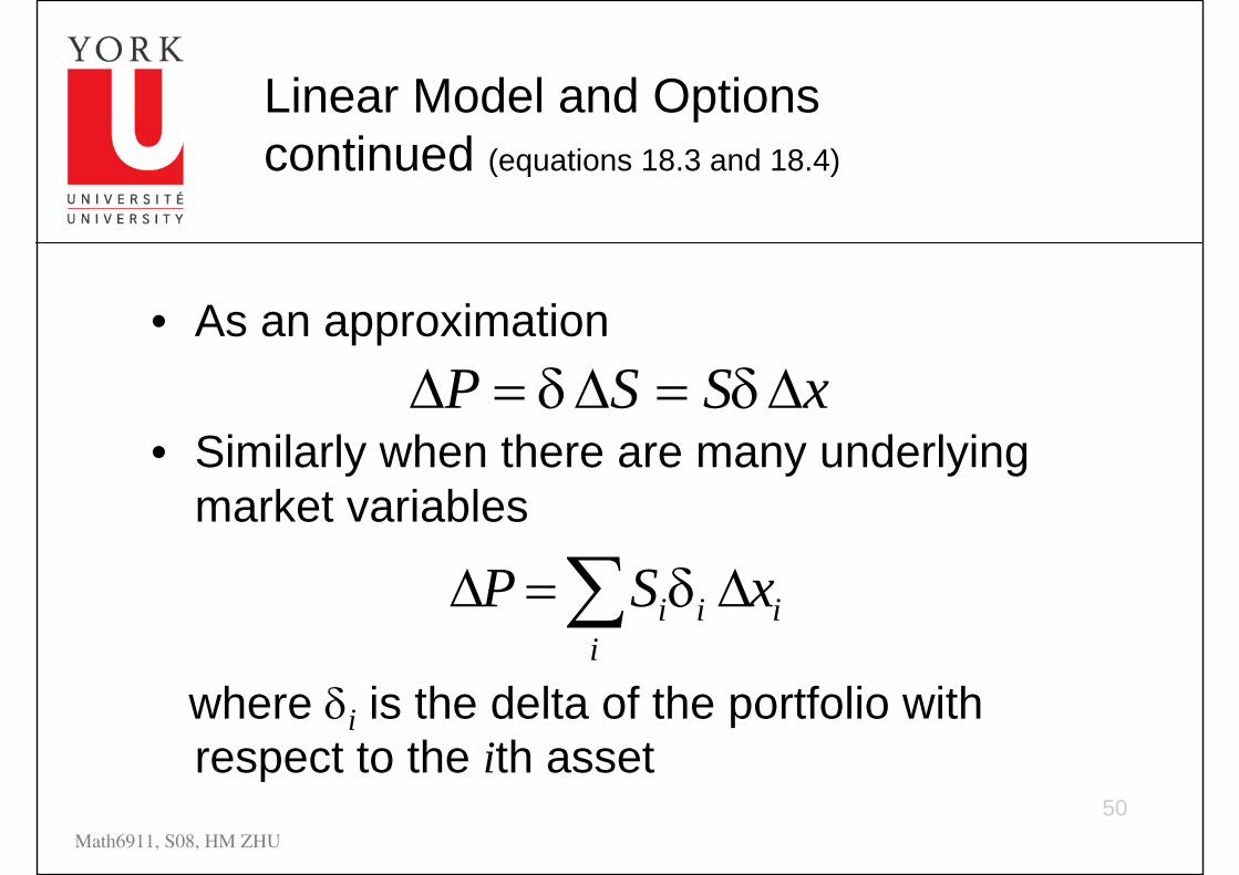
Linear Model and Options continued (equations 18.3 and 18.4)
• As an approximation
• Similarly when there are many underlying market variables
where δi is the delta of the portfolio with respect to the ith asset
xSSP ∆δ=∆δ=∆
∑ ∆δ=∆i
iii xSP
51Math6911, S08, HM ZHU
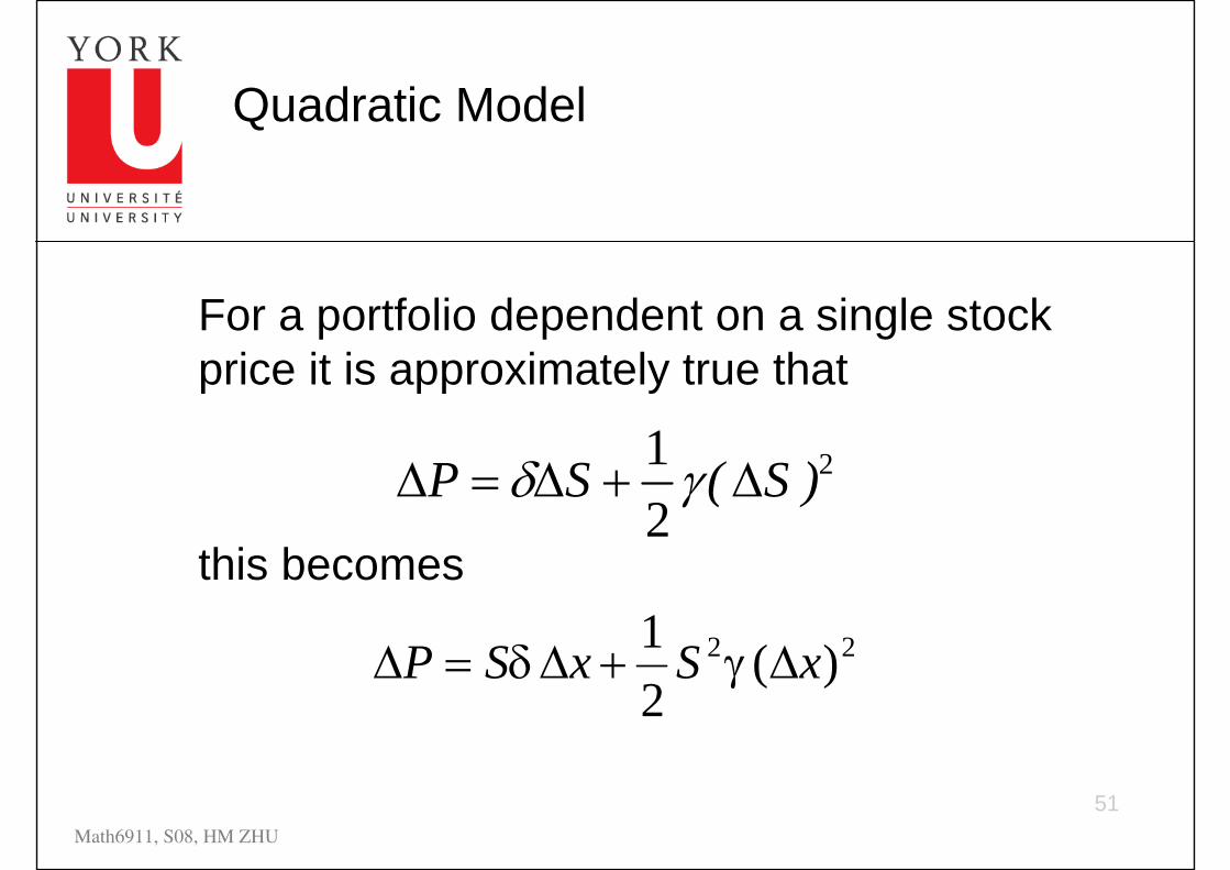
Quadratic Model
For a portfolio dependent on a single stock price it is approximately true that
this becomes
212
P S ( S )δ γ∆ = ∆ + ∆
22 )(21 xSxSP ∆γ+∆δ=∆
52Math6911, S08, HM ZHU
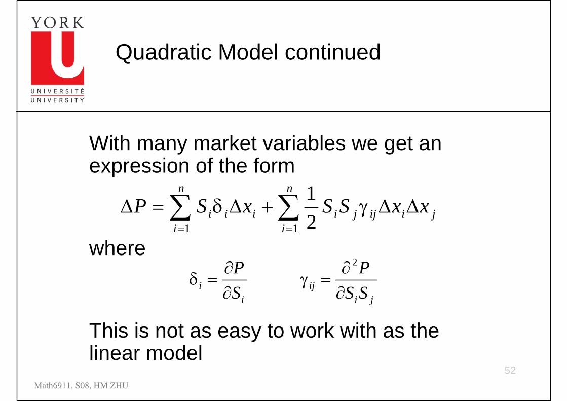
Quadratic Model continued
With many market variables we get an expression of the form
where
This is not as easy to work with as the linear model
∑ ∑= =
∆∆γ+∆δ=∆n
i
n
ijiijjiiii xxSSxSP
1 1 21
jiij
ii SS
PSP
∂∂
=γ∂∂
=δ2
53Math6911, S08, HM ZHU
Comparison of Approaches
• Historical simulation lets historical data determine distributions, but is computationally slower
• Monte Carlo simulation can handle any distribution and is easy to incorporate back and stress tests. It allows to achieve any accuracy (if the time is not an issue). It is computationally intensive.
• Model building approach assumes normal distributions for market variables. It tends to give poor results for low delta portfolios
54Math6911, S08, HM ZHU
Stress Testing
• This involves testing how well a portfolio performs under some of the most extreme market moves seen in the last 10 to 20 years
55Math6911, S08, HM ZHU
Back-Testing
• Tests how well VaR estimates would have performed in the past
• We could ask the question: How often was the actual 10-day loss greater than the 99%/10 day VaR?
Recommended