1/29/07 1
3D Transformations - II
Computer GraphicsCOMP 770 (236)Spring 2007
Instructor: Brandon Lloyd
1/29/07 2
From last time…■ Mathematical foundations
° scalar fields, vector spaces, affine spaces
° linear transformations, matrices
■ Entities° vectors, points, frames
■ Changing frames v. transforming coordinates
1/29/07 3
Outline■ Where are we going?
° Sneak peek at the rendering pipeline
■ Vector algebra° Dot product, cross product, tensor product
■ Modeling transformations° Translation, rotation, scale
■ Viewing transformation
■ Projections° Orthographic, perspective
1/29/07 4
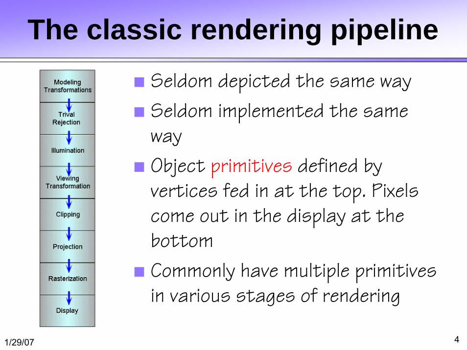
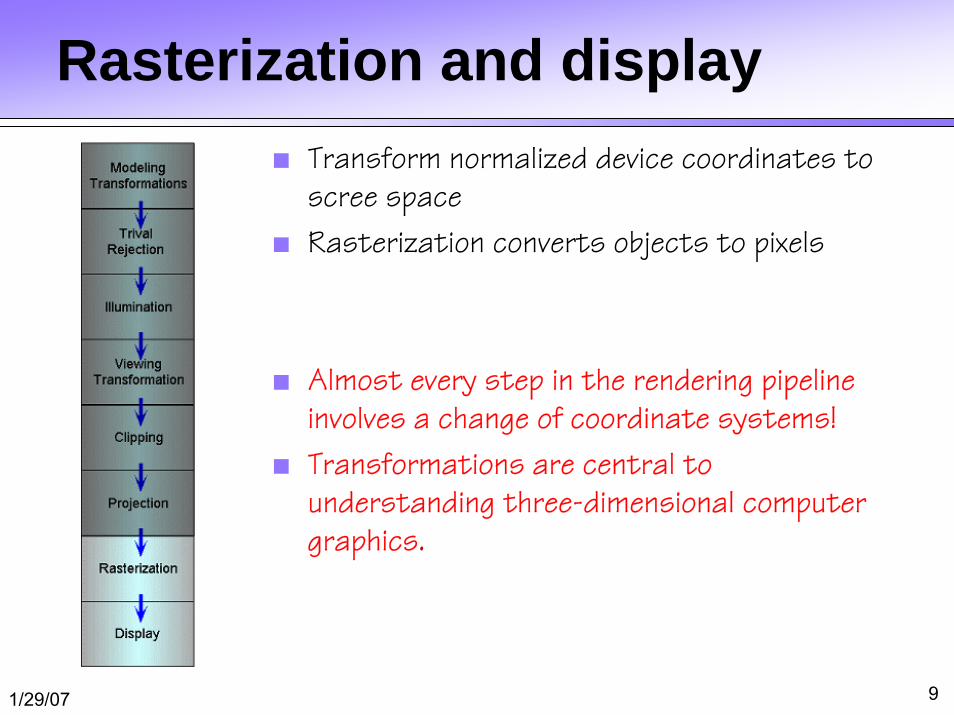
The classic rendering pipeline■ Seldom depicted the same way
■ Seldom implemented the same way
■ Object primitives defined by vertices fed in at the top. Pixels come out in the display at the bottom
■ Commonly have multiple primitivesin various stages of rendering
1/29/07 5
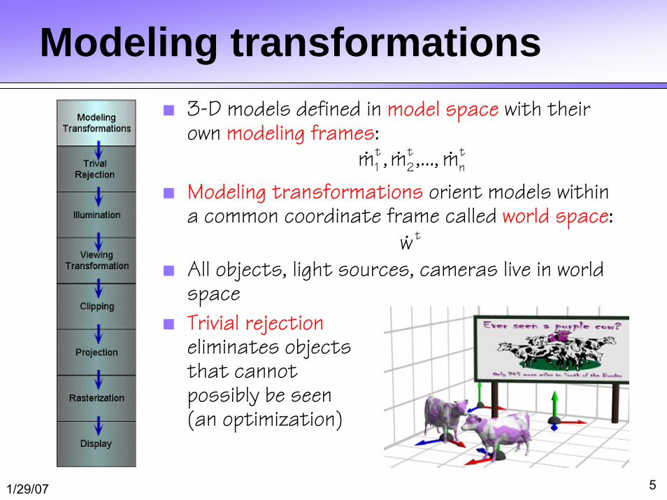
Modeling transformations■ 3-D models defined in model space with their
own modeling frames:
■ Modeling transformations orient models within a common coordinate frame called world space:
■ All objects, light sources, cameras live in world space
■ Trivial rejectioneliminates objectsthat cannotpossibly be seen(an optimization)
tn
t2
t1 m,...,m,m
tw
1/29/07 6
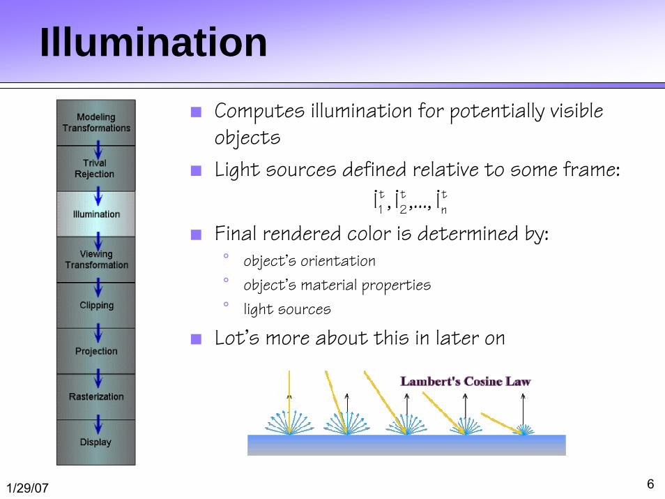
Illumination■ Computes illumination for potentially visible
objects
■ Light sources defined relative to some frame:
■ Final rendered color is determined by:° object’s orientation
° object’s material properties
° light sources
■ Lot’s more about this in later on
tn
t2
t1 l,...,l,l
1/29/07 7
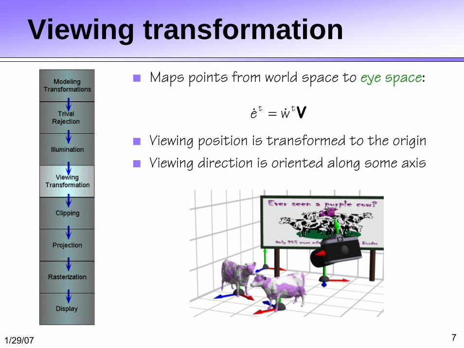
Viewing transformation■ Maps points from world space to eye space:
■ Viewing position is transformed to the origin
■ Viewing direction is oriented along some axis
Vtt we =
1/29/07 8
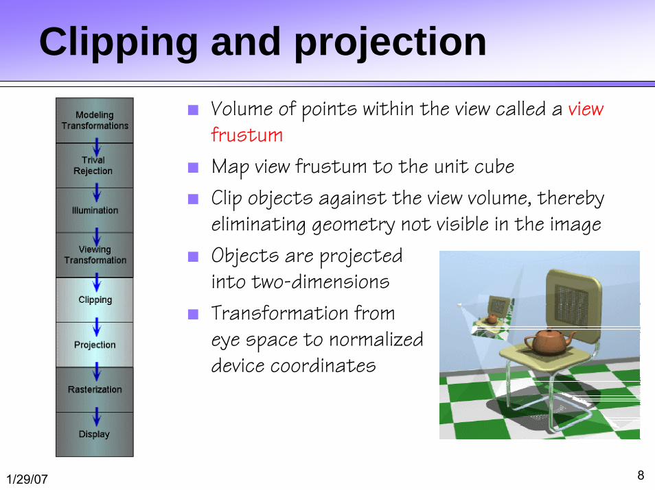
Clipping and projection■ Volume of points within the view called a view
frustum
■ Map view frustum to the unit cube
■ Clip objects against the view volume, thereby eliminating geometry not visible in the image
■ Objects are projectedinto two-dimensions
■ Transformation fromeye space to normalizeddevice coordinates
1/29/07 9
Rasterization and display■ Transform normalized device coordinates to
scree space
■ Rasterization converts objects to pixels
■ Almost every step in the rendering pipeline involves a change of coordinate systems!
■ Transformations are central to understanding three-dimensional computer graphics.
1/29/07 10
Vector algebra■ We already saw vector addition and
multiplications by a scalar
■ Three kinds of vector multiplication° Dot product ( ⋅ ) - returns a scalar
° Cross product ( × ) - returns a vector
° Tensor product ( ⊗ ) - returns a matrix
1/29/07 11
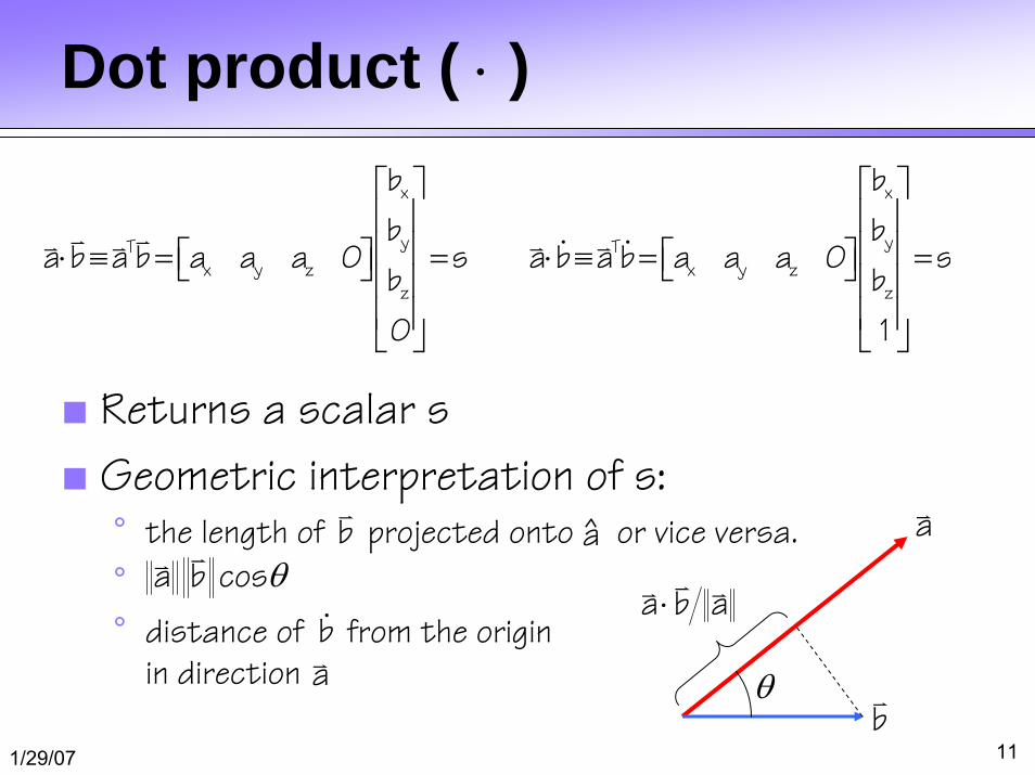
Dot product ( ⋅ )
■ Returns a scalar s
■ Geometric interpretation of s:° the length of projected onto or vice versa.
°° distance of from the origin
in direction
x x
y yT Tx y z x y z
z z
b b
b ba b a b a a a 0 s a b a b a a a 0 s
b b
0 1
⎡ ⎤ ⎡ ⎤⎢ ⎥ ⎢ ⎥⎢ ⎥ ⎢ ⎥⋅ ≡ = = ⋅ ≡ = =⎡ ⎤ ⎡ ⎤⎣ ⎦ ⎣ ⎦⎢ ⎥ ⎢ ⎥⎢ ⎥ ⎢ ⎥⎣ ⎦ ⎣ ⎦
b a
b
a
a b cosθ
θ
a
b
a b a⋅
1/29/07 12
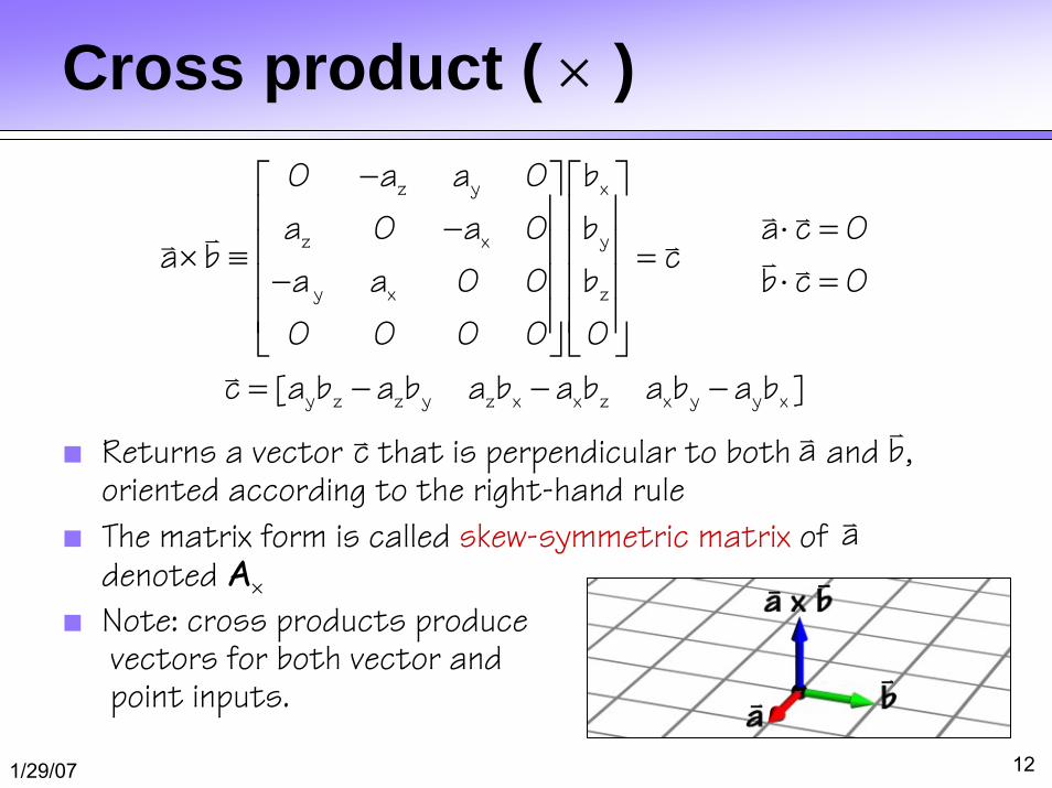
Cross product ( × )
■ Returns a vector that is perpendicular to both and , oriented according to the right-hand rule
■ The matrix form is called skew-symmetric matrix of denoted A×
■ Note: cross products producevectors for both vector andpoint inputs.
z y x
z x y
y x z
y z z y z x x z x y y x
0 a a 0 b
a 0 a 0 b a c 0a b c
a a 0 0 b b c 0
0 0 0 0 0
c [a b a b a b a b a b a b ]
−⎡ ⎤ ⎡ ⎤⎢ ⎥ ⎢ ⎥− ⋅ =⎢ ⎥ ⎢ ⎥× ≡ =− ⋅ =⎢ ⎥ ⎢ ⎥⎢ ⎥ ⎢ ⎥⎣ ⎦ ⎣ ⎦= − − −
a
a bc
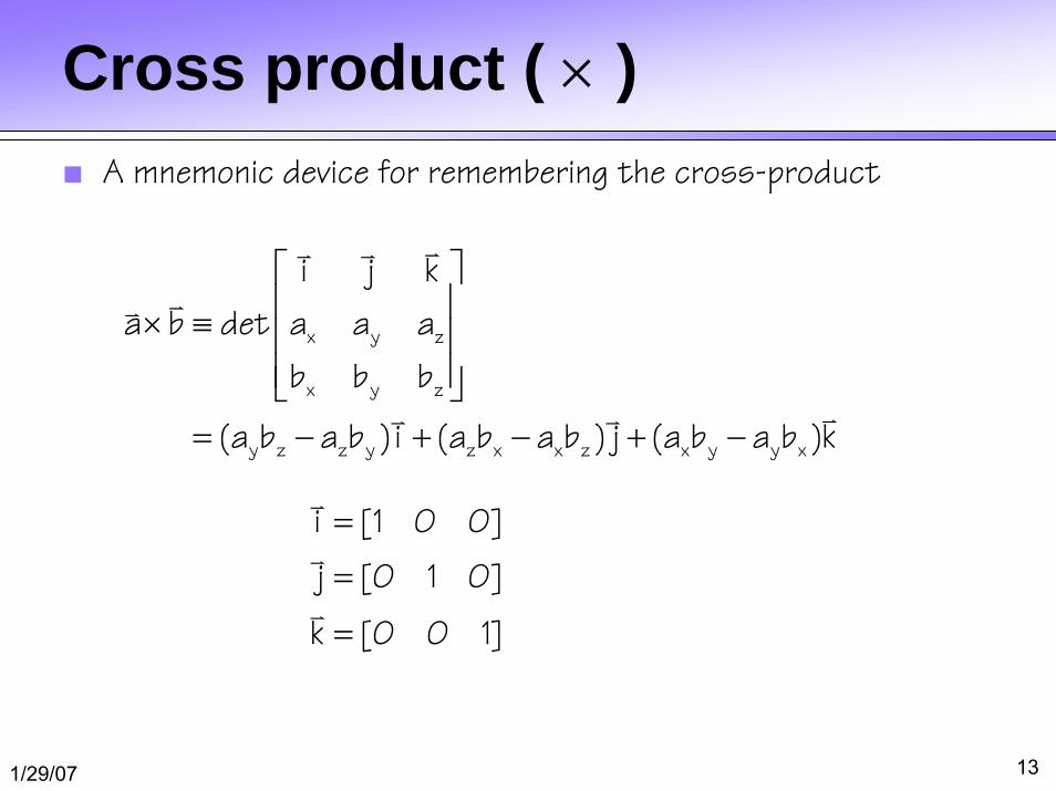
1/29/07 13
Cross product ( × )■ A mnemonic device for remembering the cross-product
x y z
x y z
y z z y z x x z x y y x
i j k
a b det a a a
b b b
(a b a b )i (a b a b ) j (a b a b )k
⎡ ⎤⎢ ⎥× ≡ ⎢ ⎥⎢ ⎥⎣ ⎦
= − + − + −
i [1 0 0]
j [0 1 0]
k [0 0 1]
=
=
=
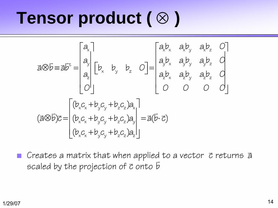
1/29/07 14
Tensor product ( ⊗ )x x x x y x z
y y x y y y ztx y z
z z x z y z z
x x y y z z x
x x y y z z y
x x y y z z z
a ab ab ab 0
a a b a b a b 0a b ab b b b 0
a a b a b a b 0
0 0 0 0 0
(b c b c b c )a
(a b)c (b c b c b c )a a(b c)
(b c b c b c )a
⎡ ⎤ ⎡ ⎤⎢ ⎥ ⎢ ⎥⎢ ⎥ ⎢ ⎥⊗ ≡ = =⎡ ⎤⎣ ⎦⎢ ⎥ ⎢ ⎥⎢ ⎥ ⎢ ⎥⎣ ⎦ ⎣ ⎦+ +⎡ ⎤
⎢ ⎥⊗ = + + = ⋅⎢ ⎥⎢ ⎥+ +⎣ ⎦
■ Creates a matrix that when applied to a vector returns scaled by the projection of onto c
ab
c
1/29/07 15
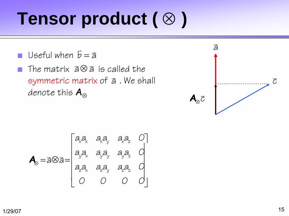
Tensor product ( ⊗ )
x x x y x z
y x y y y z
z x z y z z
a a a a a a 0
a a a a a a 0a a
a a a a a a 0
0 0 0 0
⊗
⎡ ⎤⎢ ⎥⎢ ⎥= ⊗ =⎢ ⎥⎢ ⎥⎣ ⎦
A
■ Useful when
■ The matrix is called thesymmetric matrix of . We shall
denote this A⊗
b a=a
c
c⊗A
a a⊗a
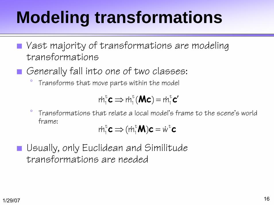
1/29/07 16
Modeling transformations■ Vast majority of transformations are modeling
transformations
■ Generally fall into one of two classes:° Transforms that move parts within the model
° Transformations that relate a local model’s frame to the scene’s world frame:
■ Usually, only Euclidean and Similitude transformations are needed
t t t1 1m (m ) w⇒ =c M c c
t t t1 1 1m m ( ) m ′⇒ =c Mc c
1/29/07 17
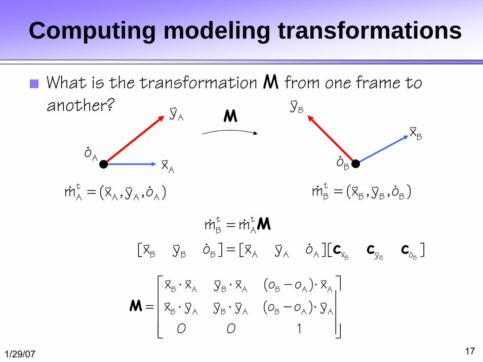
Computing modeling transformations
■ What is the transformation M from one frame to another?
Ax
Ay
AoBx
By
Bo
tB B B Bm (x , y ,o )=
M
tA A A Am (x , y ,o )=
B B B
t tB A
B B B A A A x y o
m m
[x y o ] [x y o ][ ]
==
Mc c c
B A B A B A A
B A B A B A A
x x y x (o o ) x
x y y y (o o ) y
0 0 1
⋅ ⋅ − ⋅⎡ ⎤⎢ ⎥= ⋅ ⋅ − ⋅⎢ ⎥⎢ ⎥⎣ ⎦
M
1/29/07 18
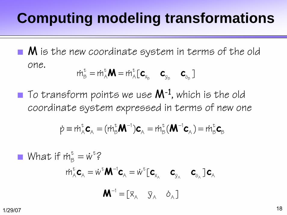
Computing modeling transformations
■ M is the new coordinate system in terms of the old one.
■ To transform points we use M-1, which is the old coordinate system expressed in terms of new one
■ What if ?
t t 1 t 1 tA A B A B A B Bp m (m ) m ( ) m− −≡ = = =c M c M c c
B B B
t t tB A A x y om m m [ ]= =M c c c
t tBm w=
A A A
t t 1 tA A A x y o Am w w [ ]−= =c M c c c c c
1A A A[x y o ]− =M
1/29/07 19
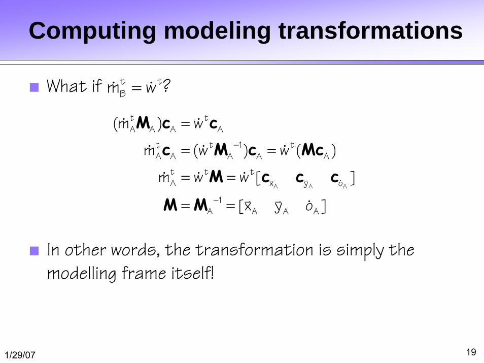
Computing modeling transformations
■ What if ?
■ In other words, the transformation is simply the
modelling frame itself!
t tBm w=
A A A
t tA A A A
t t 1 tA A A A A
t t tA x y o
1A A A A
(m ) w
m (w ) w ( )
m w w [ ]
[x y o ]
−
−
=
= =
= =
= =
M c cc M c Mc
M c c c
M M
1/29/07 20
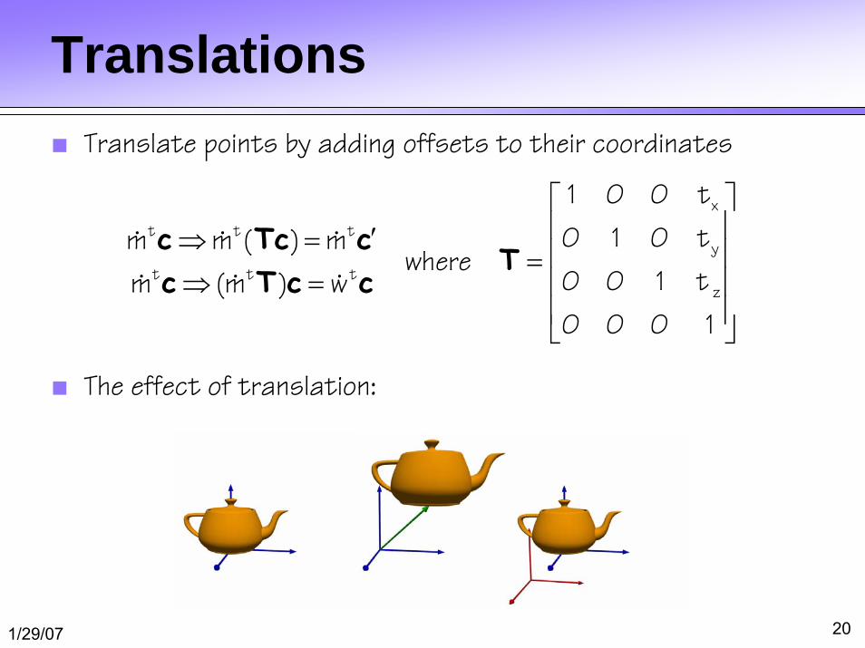
Translations■ Translate points by adding offsets to their coordinates
■ The effect of translation:
x
t t ty
t t tz
1 0 0 t
0 1 0 tm m ( ) mwhere
0 0 1 tm (m ) w
0 0 0 1
⎡ ⎤⎢ ⎥′⇒ = ⎢ ⎥=
⇒ = ⎢ ⎥⎢ ⎥⎣ ⎦
c Tc cT
c T c c
1/29/07 21
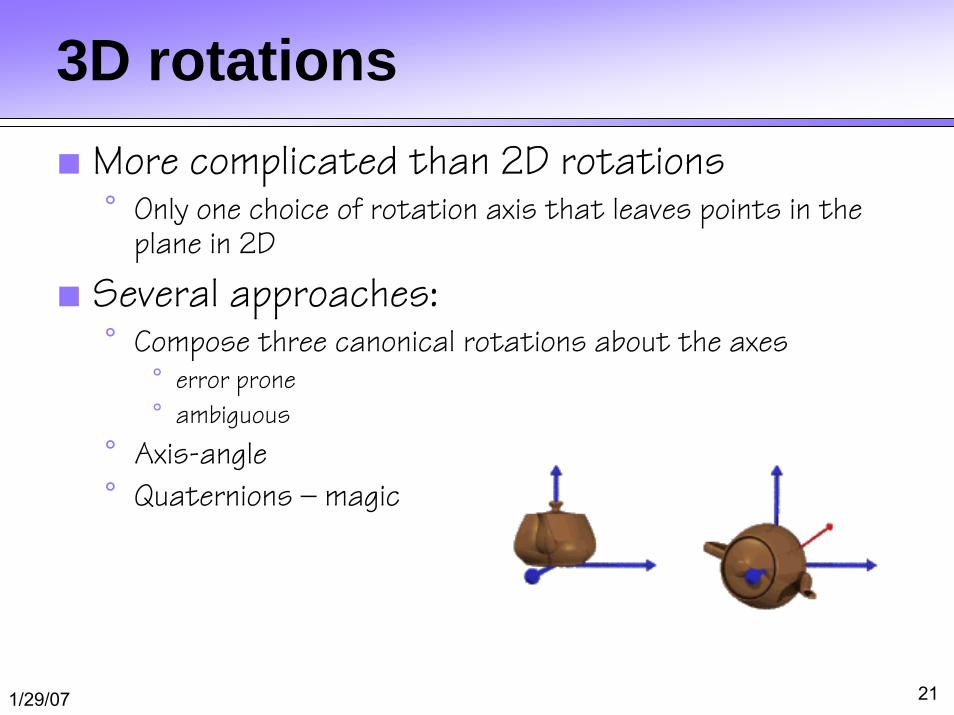
3D rotations■ More complicated than 2D rotations
° Only one choice of rotation axis that leaves points in the plane in 2D
■ Several approaches:° Compose three canonical rotations about the axes
° error prone
° ambiguous
° Axis-angle
° Quaternions – magic
1/29/07 22
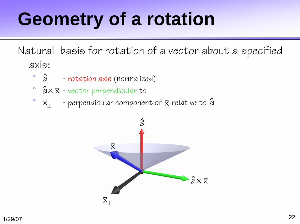
Geometry of a rotationNatural basis for rotation of a vector about a specified
axis:° - rotation axis (normalized)
° - vector perpendicular to
° - perpendicular component of relative to
a
a x×
x
x⊥
a
x⊥
a x×
x a
1/29/07 23
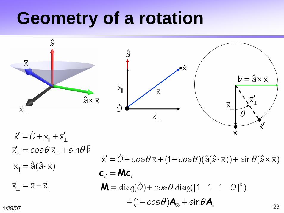
Geometry of a rotationa
x
x⊥a x×
x′x
a
xˆb a x= ×
x xx⊥′x⊥
θ0x⊥
x cos x sin bθ θ⊥ ⊥′ = +x 0 x x⊥′ ′= + +
ˆ ˆ ˆx 0 cos x (1 cos )(a(a x)) sin (a x)θ θ θ′ = + + − ⋅ + ×
tdiag(0) cos diag([1 1 1 0] )
(1 cos ) sin
θθ θ⊗ ×
= +
+ − +
MA A
ˆ ˆx a(a x)= ⋅x x′ =c Mc
x x x⊥ = −
1/29/07 24
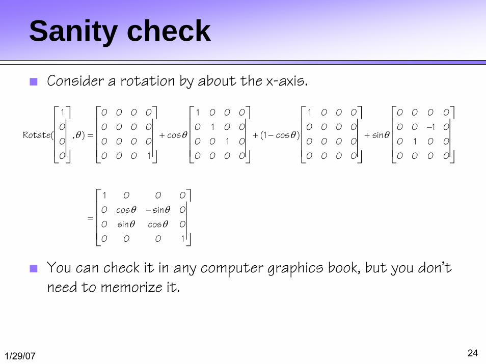
Sanity check■ Consider a rotation by about the x-axis.
■ You can check it in any computer graphics book, but you don’t need to memorize it.
1 0 0 0 0 1 0 0 0 1 0 0 0 0 0 0 0
0 0 0 0 0 0 1 0 0 0 0 0 0 0 0 1 0Rotate( , ) cos (1 cos ) sin
0 0 0 0 0 0 0 1 0 0 0 0 0 0 1 0 0
0 0 0 0 1 0 0 0 0 0 0 0 0 0 0 0 0
1 0 0 0
0 cos sin 0
0 sin cos 0
0 0 0 1
θ θ θ θ
θ θθ θ
−= + + − +
−=
⎡ ⎤ ⎡ ⎤ ⎡ ⎤ ⎡ ⎤ ⎡ ⎤⎢ ⎥ ⎢ ⎥ ⎢ ⎥ ⎢ ⎥ ⎢ ⎥⎢ ⎥ ⎢ ⎥ ⎢ ⎥ ⎢ ⎥ ⎢ ⎥⎢ ⎥ ⎢ ⎥ ⎢ ⎥ ⎢ ⎥ ⎢ ⎥⎣ ⎦ ⎣ ⎦ ⎣ ⎦ ⎣ ⎦ ⎣ ⎦
⎡ ⎤⎢ ⎥⎢ ⎥⎢ ⎥⎣ ⎦
1/29/07 25
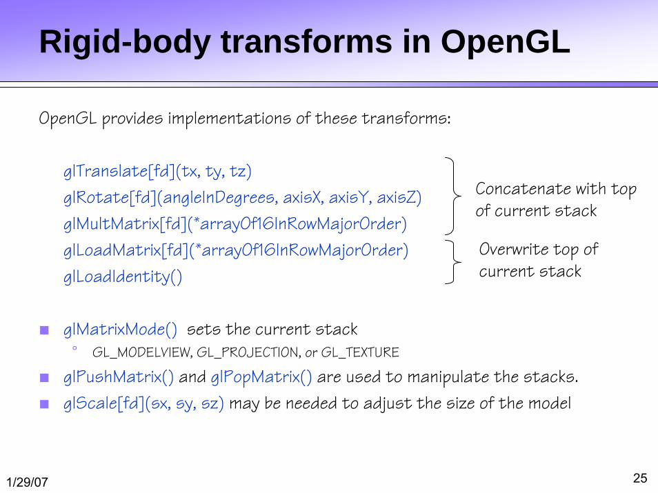
Rigid-body transforms in OpenGL
OpenGL provides implementations of these transforms:
glTranslate[fd](tx, ty, tz)
glRotate[fd](angleInDegrees, axisX, axisY, axisZ)
glMultMatrix[fd](*arrayOf16InRowMajorOrder)
glLoadMatrix[fd](*arrayOf16InRowMajorOrder)
glLoadIdentity()
■ glMatrixMode() sets the current stack
° GL_MODELVIEW, GL_PROJECTION, or GL_TEXTURE
■ glPushMatrix() and glPopMatrix() are used to manipulate the stacks.
■ glScale[fd](sx, sy, sz) may be needed to adjust the size of the model
Concatenate with topof current stack
Overwrite top of current stack
1/29/07 26
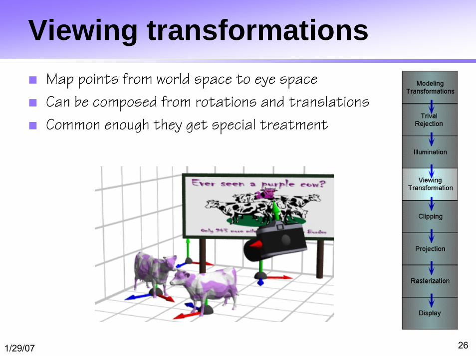
Viewing transformations■ Map points from world space to eye space
■ Can be composed from rotations and translations
■ Common enough they get special treatment
1/29/07 27
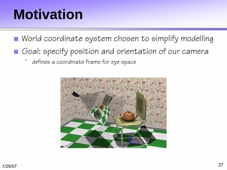
Motivation■ World coordinate system chosen to simplify modelling
■ Goal: specify position and orientation of our camera° defines a coordinate frame for eye space
1/29/07 28
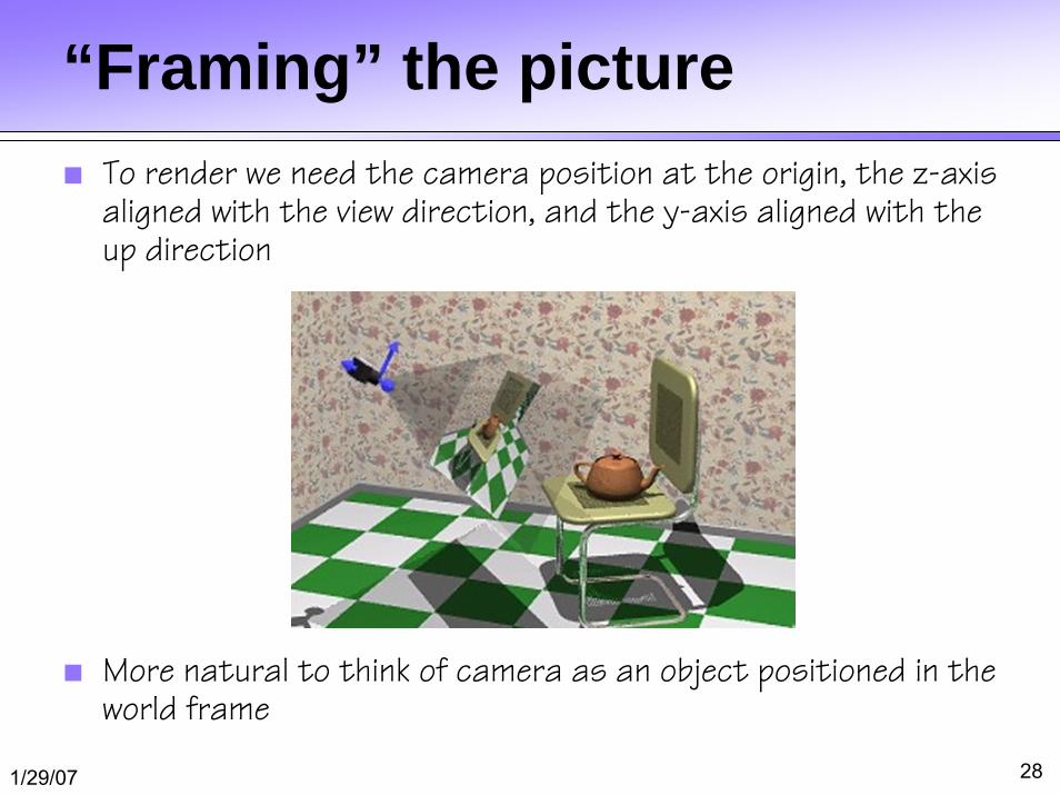
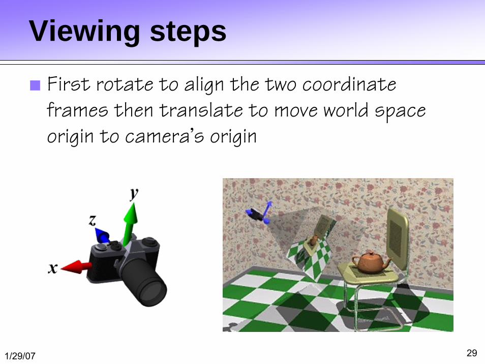
“Framing” the picture■ To render we need the camera position at the origin, the z-axis
aligned with the view direction, and the y-axis aligned with the up direction
■ More natural to think of camera as an object positioned in the world frame
1/29/07 29
Viewing steps■ First rotate to align the two coordinate
frames then translate to move world space origin to camera’s origin
1/29/07 30
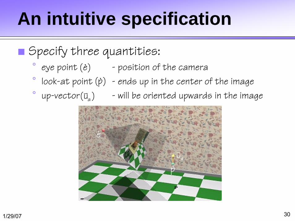
An intuitive specification■ Specify three quantities:
° eye point - position of the camera
° look-at point - ends up in the center of the image
° up-vector - will be oriented upwards in the image
(e)
(p)
a(u )
e
pau
1/29/07 31
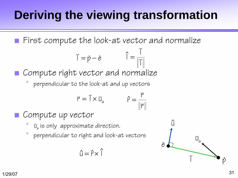
Deriving the viewing transformation
■ First compute the look-at vector and normalize
■ Compute right vector and normalize° perpendicular to the look-at and up vectors
■ Compute up vector° is only approximate direction.
° perpendicular to right and look-at vectors
l p e= −l
ll
=
ar l u= × rr
r=
ˆˆ ˆu r l= ×
au
l
e
p
au
u
1/29/07 32
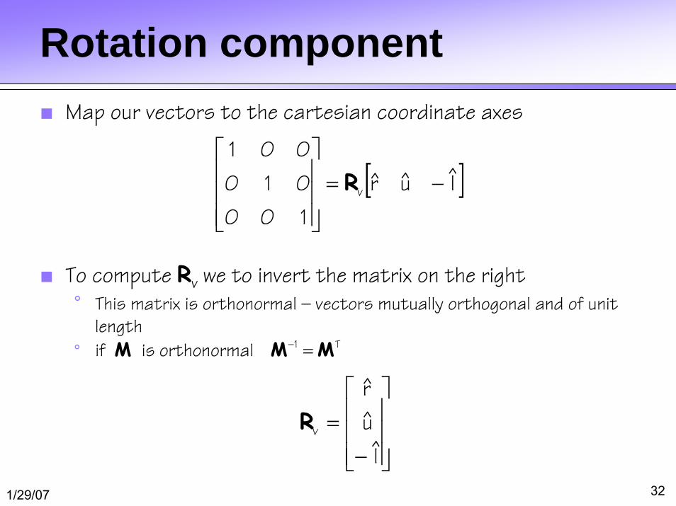
Rotation component■ Map our vectors to the cartesian coordinate axes
■ To compute Rv we to invert the matrix on the right
° This matrix is orthonormal – vectors mutually orthogonal and of unit length
°
[ ]lur
100
010
001
v −=⎥⎥⎥
⎦
⎤
⎢⎢⎢
⎣
⎡R
1 Tif is orthonormal − =M M M
⎥⎥⎥
⎦
⎤
⎢⎢⎢
⎣
⎡
−=
l
u
r
vR
1/29/07 33
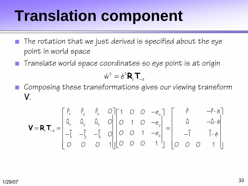
Translation component■ The rotation that we just derived is specified about the eye
point in world space
■ Translate world space coordinates so eye point is at origin
■ Composing these transformations gives our viewing transform
V.
t tv ew e −= R T
x y z x
x y z y
v ezx y z
ˆ ˆ ˆ ˆ ˆr r r 0 r r e1 0 0 e
ˆ ˆ ˆ ˆ ˆu u u 0 u u e0 1 0 e
ˆ ˆ ˆ ˆ ˆ0 0 1 el l l 0 l l e
0 0 0 10 0 0 1 0 0 0 1
−
− ⋅−⎡ ⎤ ⎡ ⎤⎡ ⎤⎢ ⎥ ⎢ ⎥⎢ ⎥ − ⋅−⎢ ⎥ ⎢ ⎥⎢ ⎥= = =⎢ ⎥ ⎢ ⎥−⎢ ⎥− − − − ⋅⎢ ⎥ ⎢ ⎥⎢ ⎥
⎣ ⎦⎢ ⎥ ⎢ ⎥⎣ ⎦ ⎣ ⎦
V R T
1/29/07 34
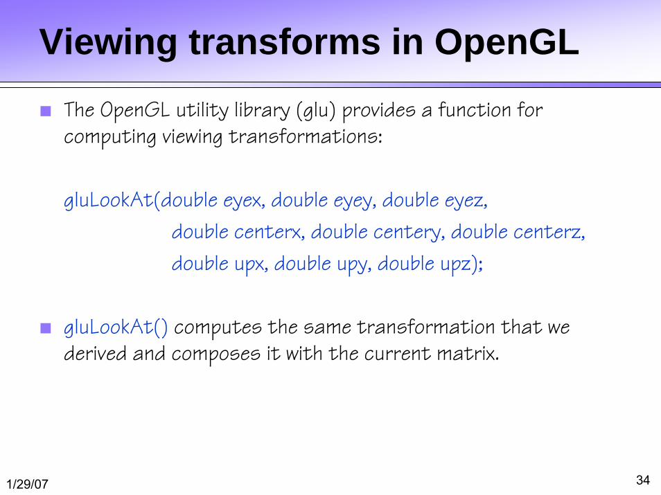
Viewing transforms in OpenGL■ The OpenGL utility library (glu) provides a function for
computing viewing transformations:
gluLookAt(double eyex, double eyey, double eyez,
double centerx, double centery, double centerz,
double upx, double upy, double upz);
■ gluLookAt() computes the same transformation that we derived and composes it with the current matrix.
1/29/07 35
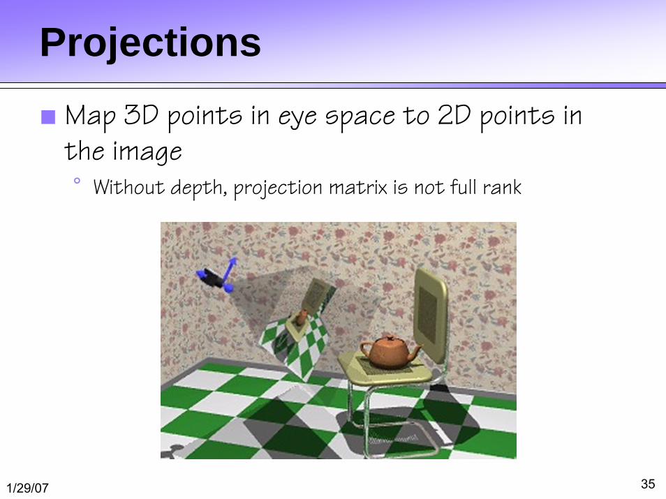
Projections■ Map 3D points in eye space to 2D points in
the image° Without depth, projection matrix is not full rank
1/29/07 36
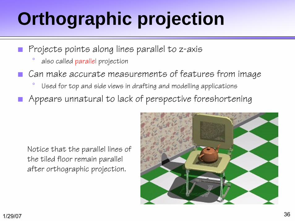
Orthographic projection■ Projects points along lines parallel to z-axis
° also called parallel projection
■ Can make accurate measurements of features from image° Used for top and side views in drafting and modelling applications
■ Appears unnatural to lack of perspective foreshortening
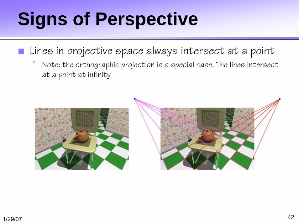
Notice that the parallel lines of the tiled floor remain parallel after orthographic projection.
1/29/07 37
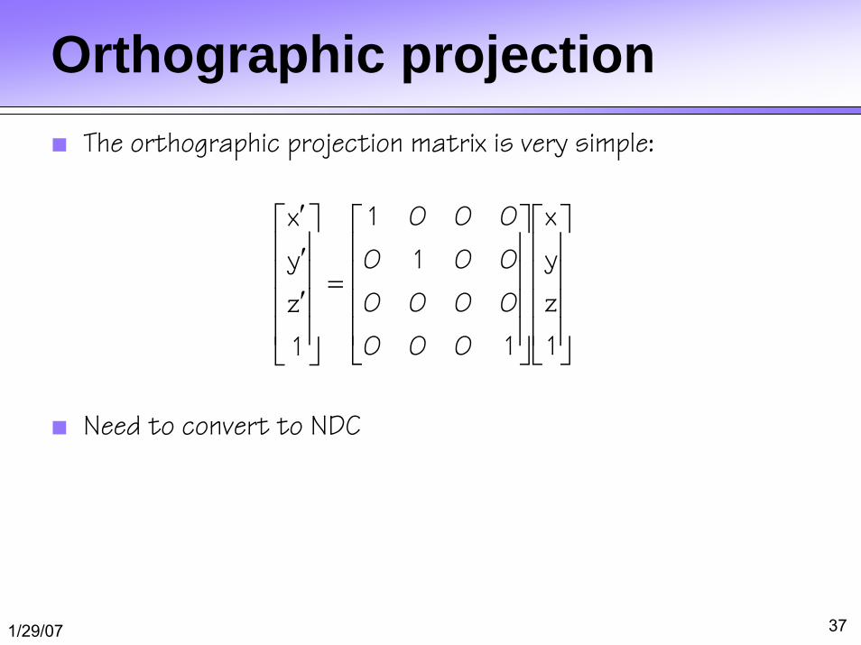
Orthographic projection■ The orthographic projection matrix is very simple:
■ Need to convert to NDC
⎥⎥⎥⎥
⎦
⎤
⎢⎢⎢⎢
⎣
⎡
⎥⎥⎥⎥
⎦
⎤
⎢⎢⎢⎢
⎣
⎡
=
⎥⎥⎥⎥
⎦
⎤
⎢⎢⎢⎢
⎣
⎡
′′′
1
z
y
x
1000
0000
0010
0001
1
z
y
x

1/29/07 38
Normalized device coordinates■ Compose projection with a scale and a translation that maps
eye coordinates to normalized device coordinates.
1/29/07 39
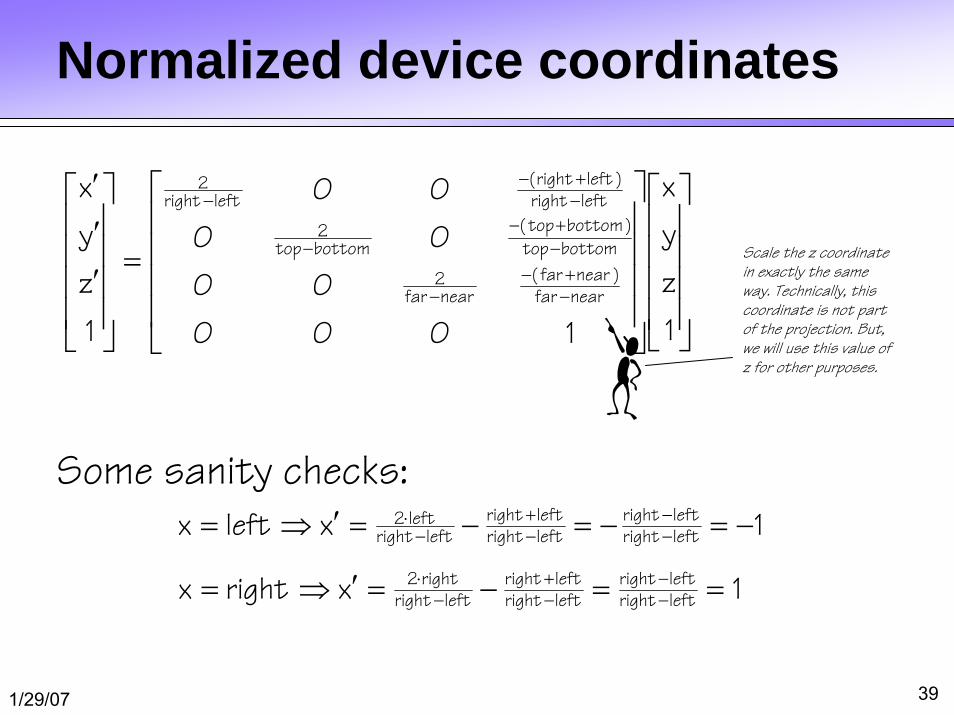
Normalized device coordinates
Some sanity checks:
⎥⎥⎥⎥
⎦
⎤
⎢⎢⎢⎢
⎣
⎡
⎥⎥⎥⎥
⎦
⎤
⎢⎢⎢⎢
⎣
⎡
=
⎥⎥⎥⎥
⎦
⎤
⎢⎢⎢⎢
⎣
⎡
′′′
−+−
−
−+−
−
−+−
−
1
z
y
x
1000
00
00
00
1
z
y
x
nearfar)nearfar(
nearfar2
bottomtop
)bottomtop(
bottomtop2
leftright)leftright(
leftright2
1xleftx leftrightleftright
leftrightleftright
leftrightleft2 −=−=−=′⇒= −
−−+
−⋅
1xrightx leftrightleftright
leftrightleftright
leftrightright2 ==−=′⇒= −
−−+
−⋅
Scale the z coordinate in exactly the same way. Technically, this coordinate is not part of the projection. But, we will use this value of z for other purposes.
1/29/07 40
Orthographic projection in OpenGL
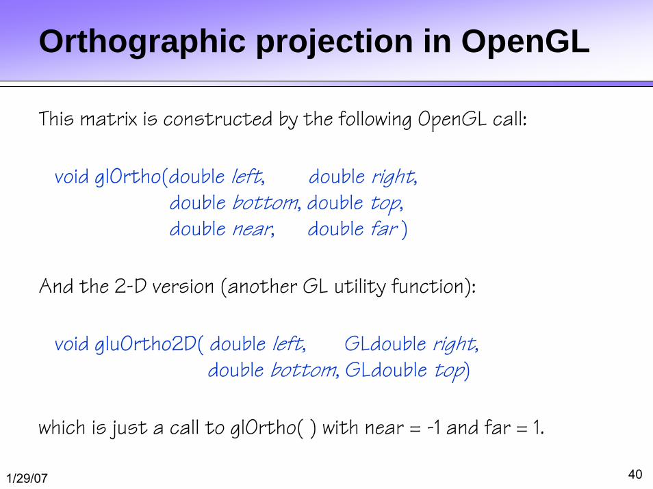
This matrix is constructed by the following OpenGL call:
void glOrtho(double left, double right,double bottom, double top, double near, double far )
And the 2-D version (another GL utility function):
void gluOrtho2D( double left, GLdouble right,double bottom, GLdouble top)
which is just a call to glOrtho( ) with near = -1 and far = 1.
1/29/07 41
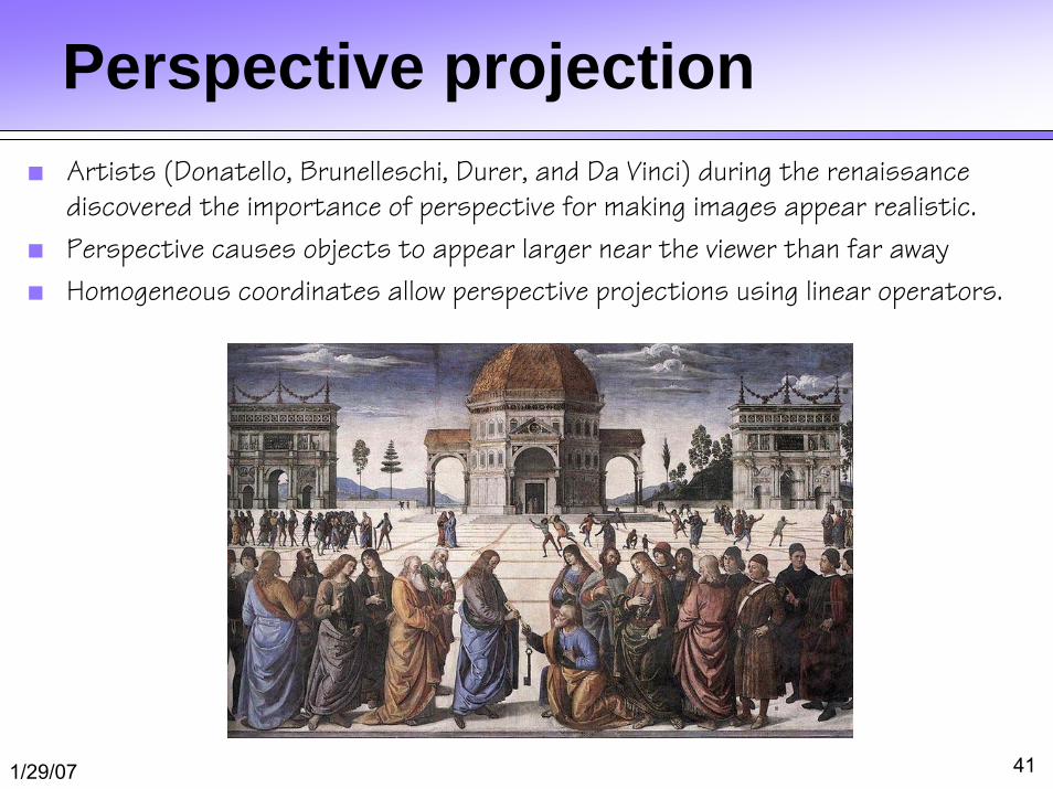
Perspective projection■ Artists (Donatello, Brunelleschi, Durer, and Da Vinci) during the renaissance
discovered the importance of perspective for making images appear realistic.
■ Perspective causes objects to appear larger near the viewer than far away
■ Homogeneous coordinates allow perspective projections using linear operators.
1/29/07 42
Signs of Perspective■ Lines in projective space always intersect at a point
° Note: the orthographic projection is a special case. The lines intersect at a point at infinity
1/29/07 43
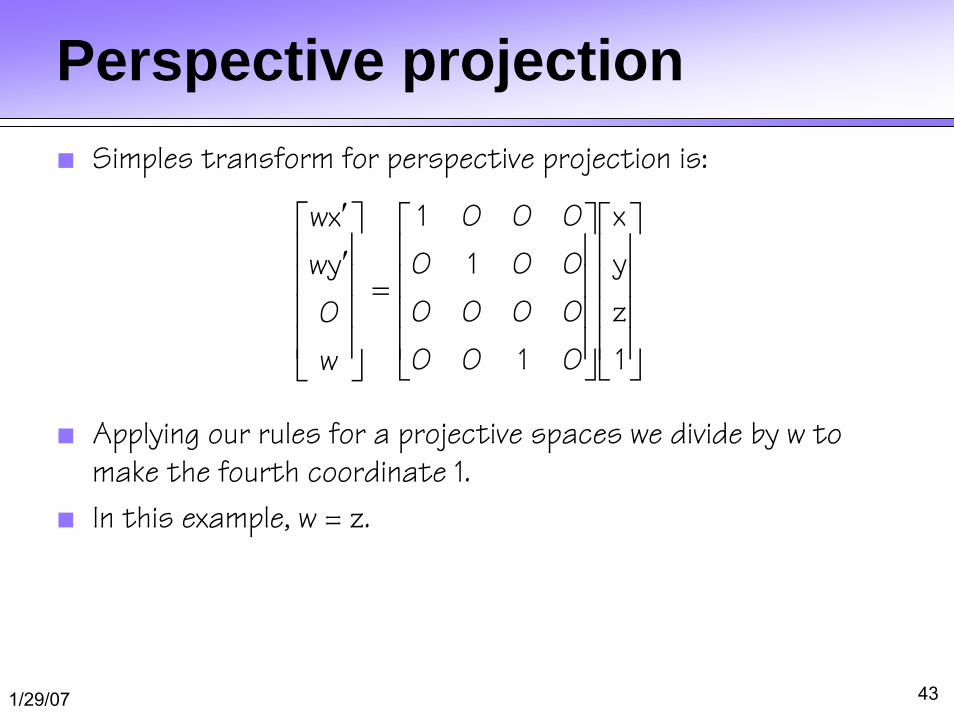
Perspective projection■ Simples transform for perspective projection is:
■ Applying our rules for a projective spaces we divide by w to make the fourth coordinate 1.
■ In this example, w = z.
⎥⎥⎥⎥
⎦
⎤
⎢⎢⎢⎢
⎣
⎡
⎥⎥⎥⎥
⎦
⎤
⎢⎢⎢⎢
⎣
⎡
=
⎥⎥⎥⎥
⎦
⎤
⎢⎢⎢⎢
⎣
⎡′′
1
z
y
x
0100
0000
0010
0001
w
0
yw
xw
1/29/07 44
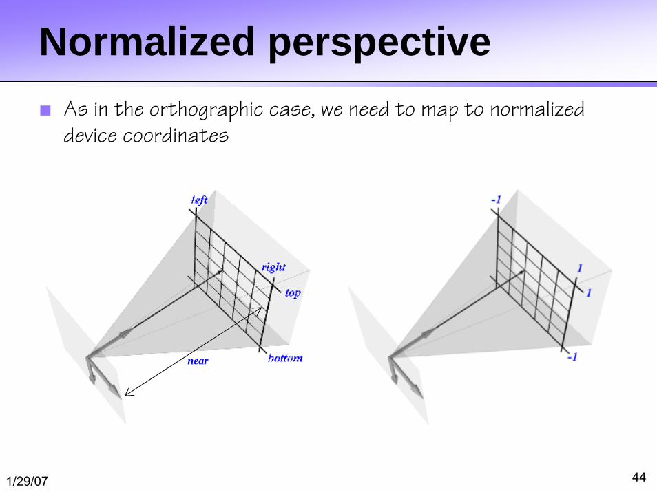
Normalized perspective■ As in the orthographic case, we need to map to normalized
device coordinates
near
1/29/07 45
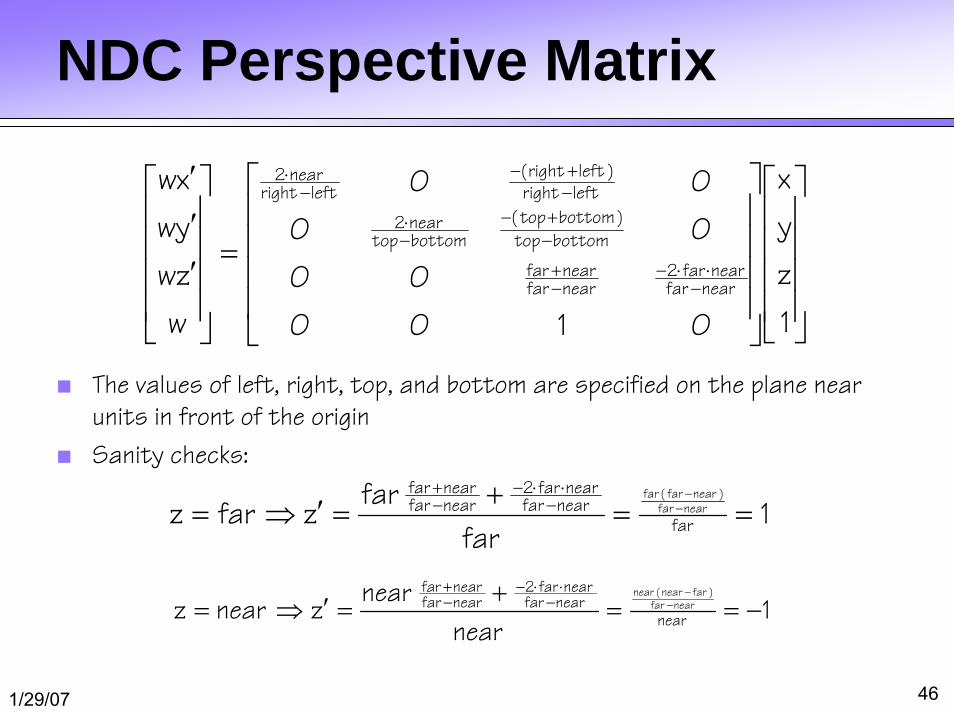
NDC Perspective Matrix
⎥⎥⎥⎥
⎦
⎤
⎢⎢⎢⎢
⎣
⎡
⎥⎥⎥⎥
⎦
⎤
⎢⎢⎢⎢
⎣
⎡
=
⎥⎥⎥⎥
⎦
⎤
⎢⎢⎢⎢
⎣
⎡
′′′
−⋅⋅−
−+
−+−
−⋅
−+−
−⋅
1
z
y
x
0100
00
00
00
w
zw
yw
xw
nearfarnearfar2
nearfarnearfar
bottomtop
)bottomtop(
bottomtopnear2
leftright)leftright(
leftrightnear2
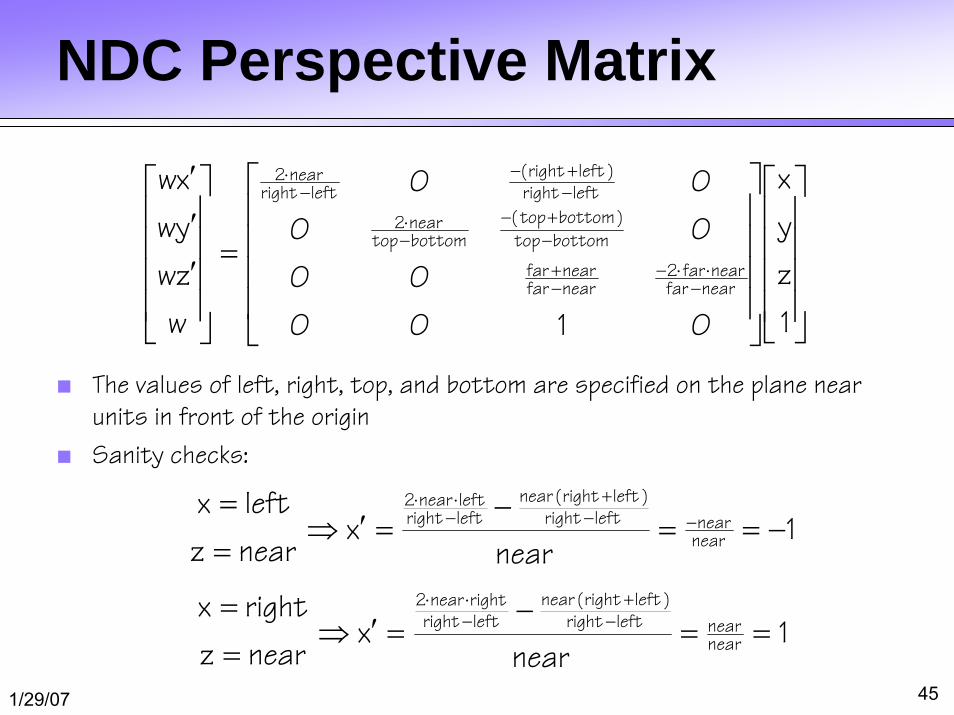
■ The values of left, right, top, and bottom are specified on the plane near units in front of the origin
■ Sanity checks:
1near
xnearz
leftxnearnearleftright
)leftright(nearleftrightleftnear2
−==−
=′⇒==
−−+
−⋅⋅
1near
xnearz
rightxnearnearleftright
)leftright(nearleftrightrightnear2
==−
=′⇒== −
+−⋅⋅
1/29/07 46
NDC Perspective Matrix
■ The values of left, right, top, and bottom are specified on the plane near units in front of the origin
■ Sanity checks:
⎥⎥⎥⎥
⎦
⎤
⎢⎢⎢⎢
⎣
⎡
⎥⎥⎥⎥
⎦
⎤
⎢⎢⎢⎢
⎣
⎡
=
⎥⎥⎥⎥
⎦
⎤
⎢⎢⎢⎢
⎣
⎡
′′′
−⋅⋅−
−+
−+−
−⋅
−+−
−⋅
1
z
y
x
0100
00
00
00
w
zw
yw
xw
nearfarnearfar2
nearfarnearfar
bottomtop
)bottomtop(
bottomtopnear2
leftright)leftright(
leftrightnear2
1far
farzfarz far
nearfarnearfar2
nearfarnearfar
nearfar)nearfar(far
==+
=′⇒= −−
−⋅⋅−
−+
1near
nearznearz near
nearfarnearfar2
nearfarnearfar
nearfar)farnear(near
−==+
=′⇒= −−
−⋅⋅−
−+
1/29/07 47
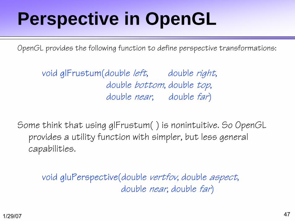
Perspective in OpenGLOpenGL provides the following function to define perspective transformations:
void glFrustum(double left, double right, double bottom, double top,double near, double far)
Some think that using glFrustum( ) is nonintuitive. So OpenGL provides a utility function with simpler, but less general capabilities.
void gluPerspective(double vertfov, double aspect,double near, double far)
1/29/07 48
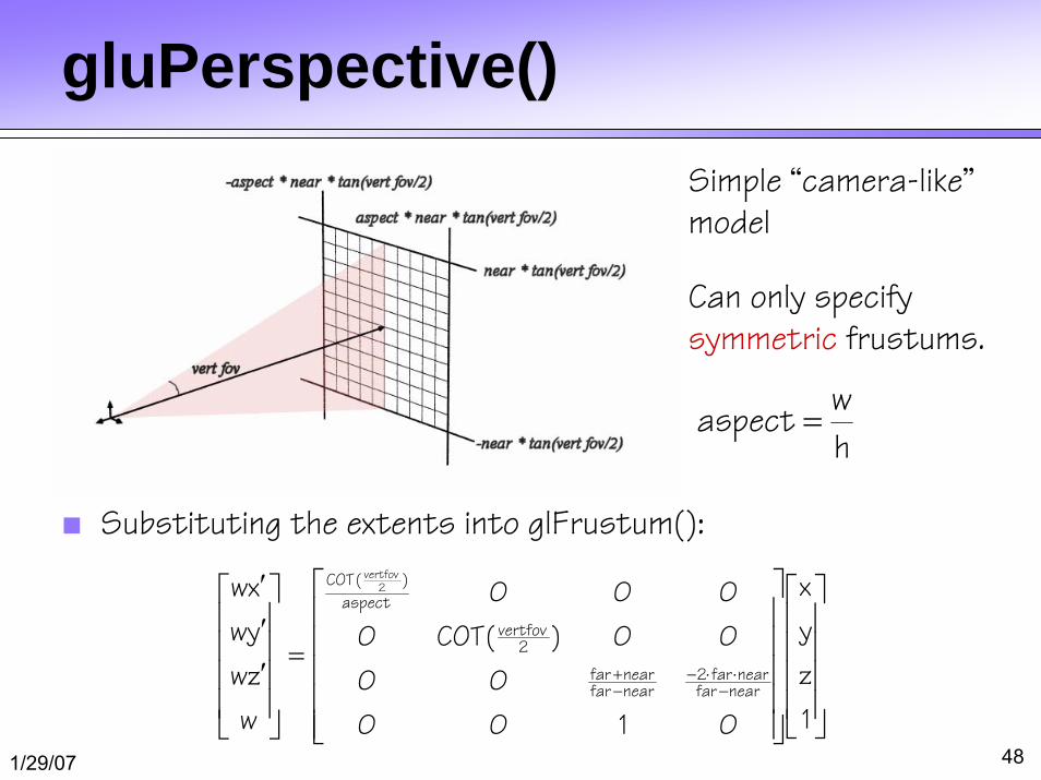
gluPerspective()
■ Substituting the extents into glFrustum():
⎥⎥⎥⎥
⎦
⎤
⎢⎢⎢⎢
⎣
⎡
⎥⎥⎥⎥⎥
⎦
⎤
⎢⎢⎢⎢⎢
⎣
⎡
=
⎥⎥⎥⎥
⎦
⎤
⎢⎢⎢⎢
⎣
⎡
′′′
−⋅⋅−
−+
1
z
y
x
0100
00
00)(COT0
000
w
zw
yw
xw
nearfarnearfar2
nearfarnearfar
2vertfov
aspect
)(COT2
vertfov
Simple “camera-like”model
Can only specify symmetric frustums.
waspect
h=
1/29/07 49
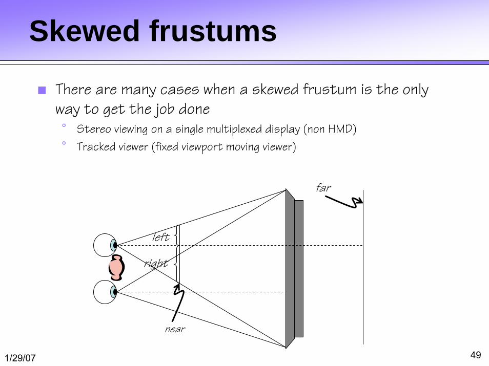
Skewed frustums
■ There are many cases when a skewed frustum is the only way to get the job done° Stereo viewing on a single multiplexed display (non HMD)
° Tracked viewer (fixed viewport moving viewer)
left
right
near
far
1/29/07 50
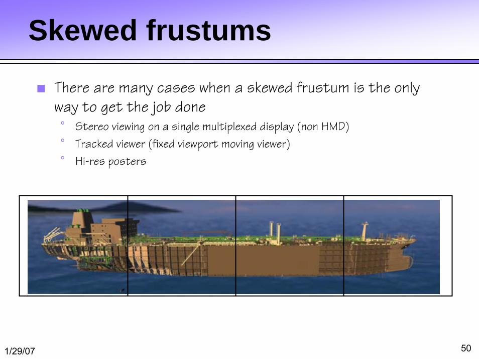
Skewed frustums
■ There are many cases when a skewed frustum is the only way to get the job done° Stereo viewing on a single multiplexed display (non HMD)
° Tracked viewer (fixed viewport moving viewer)
° Hi-res posters
1/29/07 51
Next time■ Building a 3D world
■ Picking and selection
■ 3D interaction
■ Assignment #1
Recommended