3D-PRINTED ADSORPTION MODULES FOR INDIUM RECOVERY FROM
SEAWATER BRINE
Rahman Md Arifur
Lappeenranta–Lahti University of Technology LUT
Master’s in Chemical Engineering and Water Treatment
2021
Examiner(s): Professor Eveliina Repo, D.Sc. (Tech.)
Postdoctoral Researcher Sanna Hokkanen
Abstract
Lappeenranta-Lahti University of Technology
LUT School of Engineering Science
Chemical Engineering and water treatment
Rahman Md Arifur
3D-PRINTED ADSORPTION MODULES FOR INDIUM RECOVERY FROM
SEAWATER BRINE
Master’s Thesis
2021
88 pages, 42 figures, and 5 tables
Examiners: Professor Eveliina Repo, D.Sc. (Tech.)
Postdoctoral Researcher Sanna Hokkanen,
Keywords: Indium; 3D printed TP260; Indium preconcentration; Seawater brine; Additive
manufacturing; Column adsorption; Kinetic; Isotherm
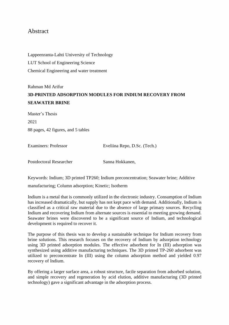
Indium is a metal that is commonly utilized in the electronic industry. Consumption of Indium
has increased dramatically, but supply has not kept pace with demand. Additionally, Indium is
classified as a critical raw material due to the absence of large primary sources. Recycling
Indium and recovering Indium from alternate sources is essential to meeting growing demand.
Seawater brines were discovered to be a significant source of Indium, and technological
development is required to recover it.
The purpose of this thesis was to develop a sustainable technique for Indium recovery from
brine solutions. This research focuses on the recovery of Indium by adsorption technology
using 3D printed adsorption modules. The effective adsorbent for In (III) adsorption was
synthesized using additive manufacturing techniques. The 3D printed TP-260 adsorbent was
utilized to preconcentrate In (III) using the column adsorption method and yielded 0.97
recovery of Indium.
By offering a larger surface area, a robust structure, facile separation from adsorbed solution,
and simple recovery and regeneration by acid elution, additive manufacturing (3D printed
technology) gave a significant advantage in the adsorption process.
Acknowledgement
I would want to appreciate and show my gratitude to my supervisor, Eveliina Repo, for
providing me with an incredible opportunity to work with her research group on an innovative
technology initiative. Her progressive encouragement, feedback, and friendly attitude (email
with smiley ) inspire me to work fearlessly. I would like to express my gratitude to my
research project partner Sea4value for the funding. I'd want to express my gratitude to my Lab
supervisor Asiia Suerbaeva for her unwavering support throughout the research time. I could
ask her any question and seek assistance without hesitation; her assistance with laboratory
work, nice demeanor, and rapid response facilitated my research work. We would like to
express our gratitude to Liisa Puro and Sanna Hokkanen for their assistance with the analysis
effort (ICP, SEM, FTIR).
I would want to express my gratitude to my wife Papia Yasmin and my entire family for their
unwavering support and understanding during my preparation of this thesis. Your prayers for
me have kept me going this far.
Finally, I want to convey my thankfulness to Allah for allowing me to overcome all obstacles.
Every day, I felt your guidance. You are the one who enabled me to complete my degree. I will
continue to place my future in your hands.
Symbol and Abbreviations
Roman characters
p pressure [bar, Pa]
R gas constant [J/kg K]
T temperature [ºC, K]
qe Equilibrium quantity of the adsorbate [mg/g]
Ce Equilibrium concentration of the adsorbate [mg/L]
Co Initial concentration of the adsorbate [mg/L]
KL Langmuir constant [L/mg]
qm Maximum adsorption capacity [mg/g]
KF Freundlich exponent [mg/g]
n Freundlich constant
Ks Sips isotherm model constant [L/g]
Ka Dissociation constant [mol/L]
qt Quantity of adsorbent adsorbed at a time t (mg ∕ g)
K1 First-order rate constant of adsorption [1/min]
t Time min
K2 Second-order rate constant of adsorption [1/min2]
Greek characters
αs Sips isotherm model constant [L/g]
βs Sips isotherm exponent
Abbreviations
AM Additive Manufacturing
BJ Binder Jetting
BET Brunauer-Emmett-Teller
CAD Computer Aided Design
CIJ Continuous Inkjet
DED Directed Energy Deposition
D2EHPA Di-(2-ethylhexyl)phosphoric acid
EDS Energy Dispersive X-Ray Spectroscopy
FTIR Fourier Transform Infrared Spectroscopy
ICP Inductive couple plasma
ITO Indium Tin Oxide
IRA-743 Amberlite® 743
LCD Liquid Crystal Display
MJ Material Jetting
PSO Pseudo-second-order model
PNP Positive Negative Positive
PA12 Polyamide 12
PBF Powder Bed Fusion
TBP Tributyl Phosphate
TFT Thin film Transistor
TP-207 Lewatit® TP-207
TP-260 Lewatit® TP-260

SEM Scanning Electron Microscopy
STL Standard Triangle Language
3D Three-dimensional, or having three dimension
Table of Contents
Abstract ...................................................................................................................................... 2
Acknowledgement ..................................................................................................................... 3
Symbol and Abbreviations ......................................................................................................... 4
1. Introduction .......................................................................................................................... 13
1.1 Background .................................................................................................................... 13
1.2 Objective of the research and contents ........................................................................... 14
2. Indium .................................................................................................................................. 15
2.1 Source and production .................................................................................................... 15
2.2 Application of Indium resource...................................................................................... 17
2.3 Supply and demand profile of Indium............................................................................ 18
3. Indium recovery techniques ................................................................................................. 20
3.1 Leaching ......................................................................................................................... 20
3.2 Pressure leaching ............................................................................................................ 22
3.3 Extraction ....................................................................................................................... 23
3.4 Electrolysis ..................................................................................................................... 24
3.5 Cementation and precipitation ....................................................................................... 25
3.6 Extraction using sub-critical water ................................................................................. 26
3.7 Extraction by supercritical fluid ..................................................................................... 27
3.8 Adsorption ...................................................................................................................... 27
4. Adsorbent materials for Indium recovery ............................................................................ 30
4.1 Resin TP-207 .................................................................................................................. 30
4.2 Resin Lewatiti® TP-260 ................................................................................................ 31
4.3 Amberlite® IRA-743 ..................................................................................................... 32
5. Additive Manufacturing ....................................................................................................... 33
5.1 Powder Bed Fusion (PBF).............................................................................................. 34
5.2 Binder Jetting (BJ) ......................................................................................................... 36
5.3 Directed Energy Deposition (DED) ............................................................................... 37
5.4 Materials Extrusion (ME)............................................................................................... 37
5.5 Materials Jetting (MJ) .................................................................................................... 38
5.6 Sheet Lamination (SL) ................................................................................................... 39
5.7 Vat Polymerization (VP) ................................................................................................ 40
6. Adsorption............................................................................................................................ 41
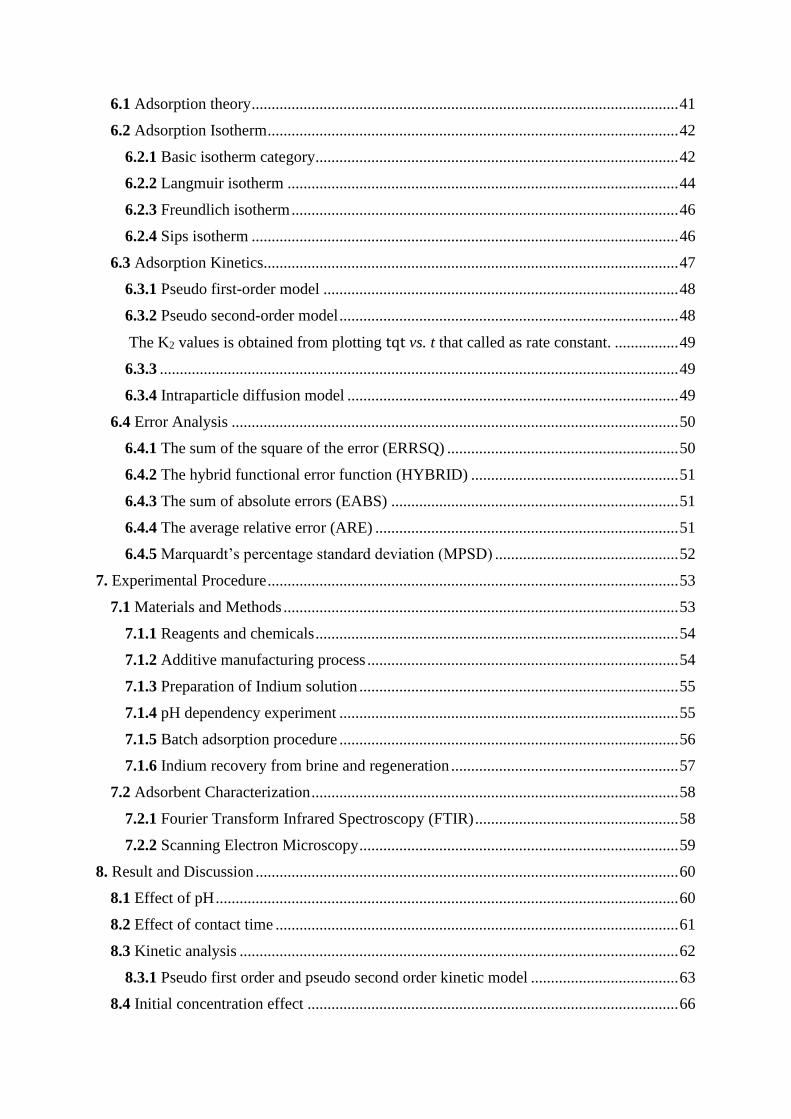
6.1 Adsorption theory ........................................................................................................... 41
6.2 Adsorption Isotherm ....................................................................................................... 42
6.2.1 Basic isotherm category ........................................................................................... 42
6.2.2 Langmuir isotherm .................................................................................................. 44
6.2.3 Freundlich isotherm ................................................................................................. 46
6.2.4 Sips isotherm ........................................................................................................... 46
6.3 Adsorption Kinetics........................................................................................................ 47
6.3.1 Pseudo first-order model ......................................................................................... 48
6.3.2 Pseudo second-order model ..................................................................................... 48
The K2 values is obtained from plotting tqt vs. t that called as rate constant. ................ 49
6.3.3 .................................................................................................................................. 49
6.3.4 Intraparticle diffusion model ................................................................................... 49
6.4 Error Analysis ................................................................................................................ 50
6.4.1 The sum of the square of the error (ERRSQ) .......................................................... 50
6.4.2 The hybrid functional error function (HYBRID) .................................................... 51
6.4.3 The sum of absolute errors (EABS) ........................................................................ 51
6.4.4 The average relative error (ARE) ............................................................................ 51
6.4.5 Marquardt’s percentage standard deviation (MPSD) .............................................. 52
7. Experimental Procedure ....................................................................................................... 53
7.1 Materials and Methods ................................................................................................... 53
7.1.1 Reagents and chemicals ........................................................................................... 54
7.1.2 Additive manufacturing process .............................................................................. 54
7.1.3 Preparation of Indium solution ................................................................................ 55
7.1.4 pH dependency experiment ..................................................................................... 55
7.1.5 Batch adsorption procedure ..................................................................................... 56
7.1.6 Indium recovery from brine and regeneration ......................................................... 57
7.2 Adsorbent Characterization ............................................................................................ 58
7.2.1 Fourier Transform Infrared Spectroscopy (FTIR) ................................................... 58
7.2.2 Scanning Electron Microscopy ................................................................................ 59
8. Result and Discussion .......................................................................................................... 60
8.1 Effect of pH .................................................................................................................... 60
8.2 Effect of contact time ..................................................................................................... 61
8.3 Kinetic analysis .............................................................................................................. 62
8.3.1 Pseudo first order and pseudo second order kinetic model ..................................... 63
8.4 Initial concentration effect ............................................................................................. 66

8.5 Adsorption Isotherms ..................................................................................................... 68
8.5.1 Langmuir Isotherm .................................................................................................. 68
8.5.2 Freundlich Isotherm ................................................................................................. 70
8.6 Indium preconcentration and regeneration ..................................................................... 71
8.7 Adsorbent characterization ............................................................................................. 72
8.7.1 Scanning Electron Microscopy ................................................................................ 72
8.7.2 Fourier Transform Infrared Spectroscopy (FTIR) analysis ..................................... 74
9. Conclusions .......................................................................................................................... 76
10. References .......................................................................................................................... 78
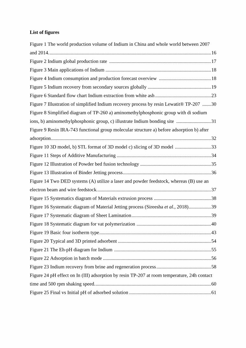
List of figures
Figure 1 The world production volume of Indium in China and whole world between 2007
and 2014. .................................................................................................................................. 16
Figure 2 Indium global production rate .................................................................................. 17
Figure 3 Main applications of Indium ..................................................................................... 18
Figure 4 Indium consumption and production forecast overview .......................................... 18
Figure 5 Indium recovery from secondary sources globally ................................................... 19
Figure 6 Standard flow chart Indium extraction from white ash ............................................. 23
Figure 7 Illustration of simplified Indium recovery process by resin Lewatit® TP-207 ....... 30
Figure 8 Simplified diagram of TP-260 a) aminomethylphosphonic group with di sodium
ions, b) aminomethylphosphonic group, c) illustrate Indium bonding site ............................ 31
Figure 9 Resin IRA-743 functional group molecular structure a) before adsorption b) after
adsorption ................................................................................................................................. 32
Figure 10 3D model, b) STL format of 3D model c) slicing of 3D model ............................. 33
Figure 11 Steps of Additive Manufacturing ............................................................................ 34
Figure 12 Illustration of Powder bed fusion technology ......................................................... 35
Figure 13 Illustration of Binder Jetting process ....................................................................... 36
Figure 14 Two DED systems (A) utilize a laser and powder feedstock, whereas (B) use an
electron beam and wire feedstock. ........................................................................................... 37
Figure 15 Systematics diagram of Materials extrusion process .............................................. 38
Figure 16 Systematic diagram of Material Jetting process (Sireesha et al., 2018) .................. 39
Figure 17 Systematic diagram of Sheet Lamination ................................................................ 39
Figure 18 Systematic diagram for vat polymerization ............................................................ 40
Figure 19 Basic four isotherm type .......................................................................................... 43
Figure 20 Typical and 3D printed adsorbent ........................................................................... 54
Figure 21 The Eh-pH diagram for Indium .............................................................................. 55
Figure 22 Adsorption in batch mode ....................................................................................... 56
Figure 23 Indium recovery from brine and regeneration process ............................................ 58
Figure 24 pH effect on In (III) adsorption by resin TP-207 at room temperature, 24h contact
time and 500 rpm shaking speed. ............................................................................................. 60
Figure 25 Final vs Initial pH of adsorbed solution .................................................................. 61
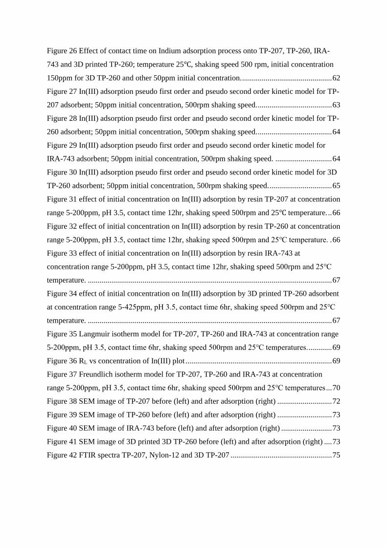
Figure 26 Effect of contact time on Indium adsorption process onto TP-207, TP-260, IRA-
743 and 3D printed TP-260; temperature 25℃, shaking speed 500 rpm, initial concentration
150ppm for 3D TP-260 and other 50ppm initial concentration. .............................................. 62
Figure 27 In(III) adsorption pseudo first order and pseudo second order kinetic model for TP-
207 adsorbent; 50ppm initial concentration, 500rpm shaking speed. ...................................... 63
Figure 28 In(III) adsorption pseudo first order and pseudo second order kinetic model for TP-
260 adsorbent; 50ppm initial concentration, 500rpm shaking speed. ...................................... 64
Figure 29 In(III) adsorption pseudo first order and pseudo second order kinetic model for
IRA-743 adsorbent; 50ppm initial concentration, 500rpm shaking speed. ............................. 64
Figure 30 In(III) adsorption pseudo first order and pseudo second order kinetic model for 3D
TP-260 adsorbent; 50ppm initial concentration, 500rpm shaking speed. ................................ 65
Figure 31 effect of initial concentration on In(III) adsorption by resin TP-207 at concentration
range 5-200ppm, pH 3.5, contact time 12hr, shaking speed 500rpm and 25℃ temperature. .. 66
Figure 32 effect of initial concentration on In(III) adsorption by resin TP-260 at concentration
range 5-200ppm, pH 3.5, contact time 12hr, shaking speed 500rpm and 25℃ temperature. . 66
Figure 33 effect of initial concentration on In(III) adsorption by resin IRA-743 at
concentration range 5-200ppm, pH 3.5, contact time 12hr, shaking speed 500rpm and 25℃
temperature. ............................................................................................................................. 67
Figure 34 effect of initial concentration on In(III) adsorption by 3D printed TP-260 adsorbent
at concentration range 5-425ppm, pH 3.5, contact time 6hr, shaking speed 500rpm and 25℃
temperature. ............................................................................................................................. 67
Figure 35 Langmuir isotherm model for TP-207, TP-260 and IRA-743 at concentration range
5-200ppm, pH 3.5, contact time 6hr, shaking speed 500rpm and 25℃ temperatures. ............ 69
Figure 36 RL vs concentration of In(III) plot ........................................................................... 69
Figure 37 Freundlich isotherm model for TP-207, TP-260 and IRA-743 at concentration
range 5-200ppm, pH 3.5, contact time 6hr, shaking speed 500rpm and 25℃ temperatures ... 70
Figure 38 SEM image of TP-207 before (left) and after adsorption (right) ............................ 72
Figure 39 SEM image of TP-260 before (left) and after adsorption (right) ............................ 73
Figure 40 SEM image of IRA-743 before (left) and after adsorption (right) .......................... 73
Figure 41 SEM image of 3D printed 3D TP-260 before (left) and after adsorption (right) .... 73
Figure 42 FTIR spectra TP-207, Nylon-12 and 3D TP-207 .................................................... 75

List of Table
Table 1 Seawater brine composition ........................................................................................ 57
Table 2 Pseudo first and pseudo second order kinetic model calculated parameter for In(III)
adsorption with TP-207, TP-260 IRA-743 and 3D TP-260 adsorbent .................................... 65
Table 3 Langmuir and Freudlich isotherm model predicted parameter value ......................... 69
Table 4 Comparative study table ............................................................................................. 71
Table 5 In(III) preconcentration data ....................................................................................... 71
13
1. Introduction
This chapter discusses the history of research into Indium recovery using adsorption
technology, includes an outline of the thesis's aim, and lists the thesis's relevant topics.
1.1 Background
Numerous electrical gadgets, the military, and a few other sectors make extensive use of
Indium and Indium-based compounds, and the European Commission defines Indium as a
critical strategic meta (Alguacil et al., 2016). Researchers are concentrating their efforts on
green energy to save fossil fuels and ensure the sustainability of the environment; solar energy
is the primary source of green energy among others (Lahtinen et al., 2017). The substantial
performance of Indium-based compounds (copper Indium gallium selenide) in solar energy
systems piques the researcher's interest—this project will soon require Indium (Sasaki, Oshima
and Baba, 2017). However, the supply of Indium is limited due to the rarity of significant
Indium-containing minerals. According to research, the amount of Indium found in nature as
ore is extremely limited (4 to 10%); also, due to Indium's low recycling rate, its price has risen
dramatically. To satisfy the growing demand for Indium and to ensure sustainability,
manufacturing capacity must be expanded and recycling rates increased, as Indium ion has a
carcinogenic impact that is damaging to the heart, kidneys, and liver.(Deferm et al., 2017)
There are a few distinct techniques for recovering and recycling metals: Leaching, solvent
extraction, ion exchange, electrolysis, cementation and precipitation, sub-critical water, and
sub-critical fluid extraction (Pradhan, Panda and Sukla, 2017). Recent approaches, on the other
hand, are not ecologically sustainable or cost-effective. The research discovered that the
adsorption approach has the potential to overcome the prior technical barriers by providing
more efficient selective recovery than other traditional methods.(F. Li et al., 2018; M. Li et al.,
2018) Unfortunately, adsorption has a limited selectivity for Indium adsorption, necessitating
additional adsorbent modifications.
Ion exchange resins are frequently utilized in the fabrication of a wide range of commercial
resins, including Amberlite IRC748 and Lewatit TP-260, TP-207, and TP-208. Several
adsorption investigations employing commercial resins for Indium recovery were conducted.
14
Recovery of Indium from the adsorbent using H2SO4/HCl elution yielded up to 99.5 percent
Indium (M. C.B. Fortes, Martins and Benedetto, 2007; Jeon, Cha and Choi, 2015).
Over the last few decades, 3D printing processes and materials have been developed to create
sophisticated mechanical structures utilizing resins, metals, and other compounds to include
functional groups into the design. 3D printing is gaining popularity as a method for
manufacturing ion exchange membranes, antimicrobial composites, and catalytically active
materials. While the traditional adsorption technique utilizes a common adsorbent to adsorb
metal ions, recycling the adsorbent and metal extraction from the adsorbent is not
straightforward. On the other hand, 3D printed adsorbents do not require filtration because they
are immersed in metal solution to absorb metals, and then Indium extraction and regeneration
are done by simple elution. The purpose of this thesis is to develop an additively manufactured
3D printed adsorbent for the recovery of Indium from saltwater. The additive manufacturing
process will be utilized to create 3D printed adsorbent. SEM, FTIR, BET, and XPS will be
utilized to characterize the adsorbent, while ICP will be used to monitor the adsorption process.
1.2 Objective of the research and contents
The objective of this thesis was to design Indium selective an additively manufactured
adsorbent using mixture of commercial resin and printing polymer.
To evaluate the efficient adsorption capacities of granular ion exchange materials and 3D
printed resins, the following batch study was conducted at the LUT university laboratory: pH
sensitivity test, batch isotherm, kinetics analysis, selectivity analysis, and regeneration
analysis. ICP analysis was used to define the concentration of Indium. characterization of the
adsorbent was conducted using FTIR for identifying the surface functional groups, SEM
analysis to see the surface morphology, EDS for elemental analysis, and BET for measuring
the surface area of the adsorbent.
A short theoretical overview reported in this work includes the Indium production, and demand,
as well as Indium recovery routes and its various applications. Theories behind of conventional
Indium recovery technologies, additive manufacturing, and adsorption methods are also
discussed. Results and discussion section collects all the obtained data as well as interpretation
and comparison of the results.
15
2. Indium
In 1863, Ferdinand Reich and Hieronymous Richter discovered Indium. They discovered it
using spectroscopy; an indigo blue line formed throughout the experiment, indicating the
presence of Indium. Indium was later referred to as Indium due to its origins in the indigo blue
line (Haynes, W.M, Lide, 2010). Indium is a chemical element with the atomic number 49 and
an electronic structure [Kr] 4d105S25P1. It is found in group 13, period 5, and block p of the
periodic table. (Alfantazi, A.M.; Moskalyk, 2003) Indium appears silvery-white color that is a
highly ductile post-transition metal having a bright luster. It is soft like sodium and has a lower
melting point of 156.60 ℃ and a boiling point of 2072℃. Indium has a density of 7.31g/cm3,
which is higher than that of gallium, and it acts as a superconductor at the critical temperature.
(Haynes, W.M, Lide, 2010). The most common Indium ionization states are In(I) and In(III),
where In(I) elements are referred to as strong reducing agents and Indium (III) elements have
decreased stability and are no longer acting as oxidizing agents. (Greenwood, N.N.; Earnshaw,
1997)
In 1924, Indium was widely employed as a nonferrous metal (French, 1934). Indium was
largely utilized as a coating material in high-performance aircraft bearings during World War
II to avoid corrosion and wear-related damage, but this use is no longer frequently used in this
industry (Greenwood, N.N.; Earnshaw, 1997). In the 1950s, a PNP transistor was constructed
using a trace quantity of Indium. Indium phosphide and Indium tin oxide were developed as
semiconducting materials for usage as thin film coatings in liquid crystal displays during the
mid-1980s and late 1980s (LCDs). Thin film technique for those materials gained popularity
in 1992 and is being utilized today across the world. (Downs, 1993)
2.1 Source and production
Indium does not have primary raw ore sources in earth’s crust. It is retrieved as by product
during processing of other metal’s ore such as zinc sulfide and copper sulfide (Frenzel, Max;
Mikolajczak, Claire; Reuter, Markus A.; Gutzmer, 2017). Indium compounds are transferred
to the iron-rich residuals in the zinc refining processing plant. Depending on the extraction
mode used in the smelter processing, different types of technologies are used to extract Indium
from the residue and electrolysis is used as a final treatment technology for further purification
16
(Alfantazi, A.M.; Moskalyk, 2003) (Frenzel, Max; Mikolajczak, Claire; Reuter, Markus A.;
Gutzmer, 2017).
The amount of Indium produced is proportional to the pace of zinc and copper sulfite
production, since Indium is a byproduct of those ores, hence the phrase supply potential is used
to describe the availability of Indium. The supply potential indicates the quantity of Indium
that can be taken from mother resources in a given year based on current market conditions.
According to the supply potential study, the existing Indium production capacity at the zinc
sulfite and copper sulfite plants is expected to be 1300 tonnes/yr and 20 tonnes/yr, respectively.
(Frenzel, Max; Tolosana-Delgado, Raimon; Gutzmer, 2015; Frenzel, Max; Mikolajczak,
Claire; Reuter, Markus A.; Gutzmer, 2017).
According to the 2016 production report, China dominates the global market, producing
approximately 290 tons of Indium, followed by South Korea, Japan, and Canada. Teck resource
limited is another large company that operates an Indium production facility in Trail, British
Columbia, with annual production volumes of 32.5, 41.8, and 36.1 tons in 2005, 2004, and
2003, respectively. (USGS, 2017)
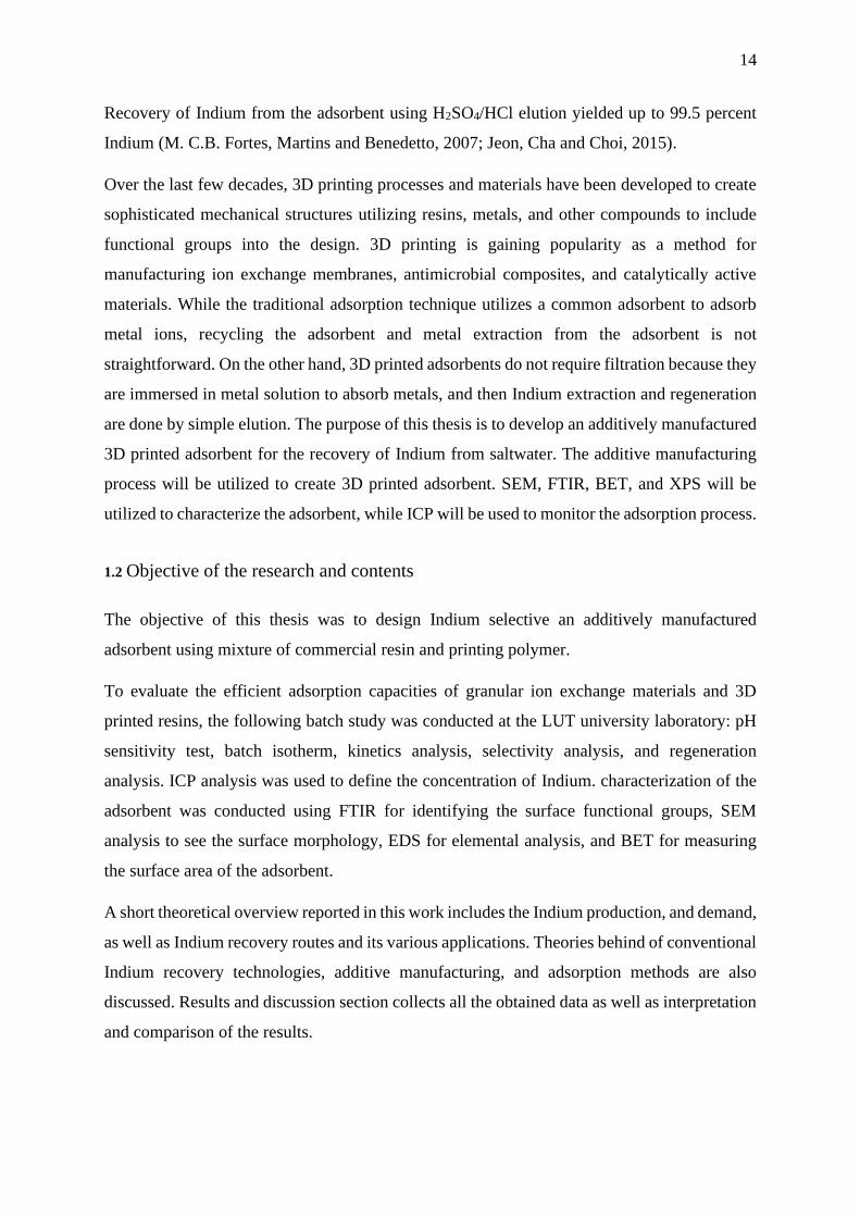
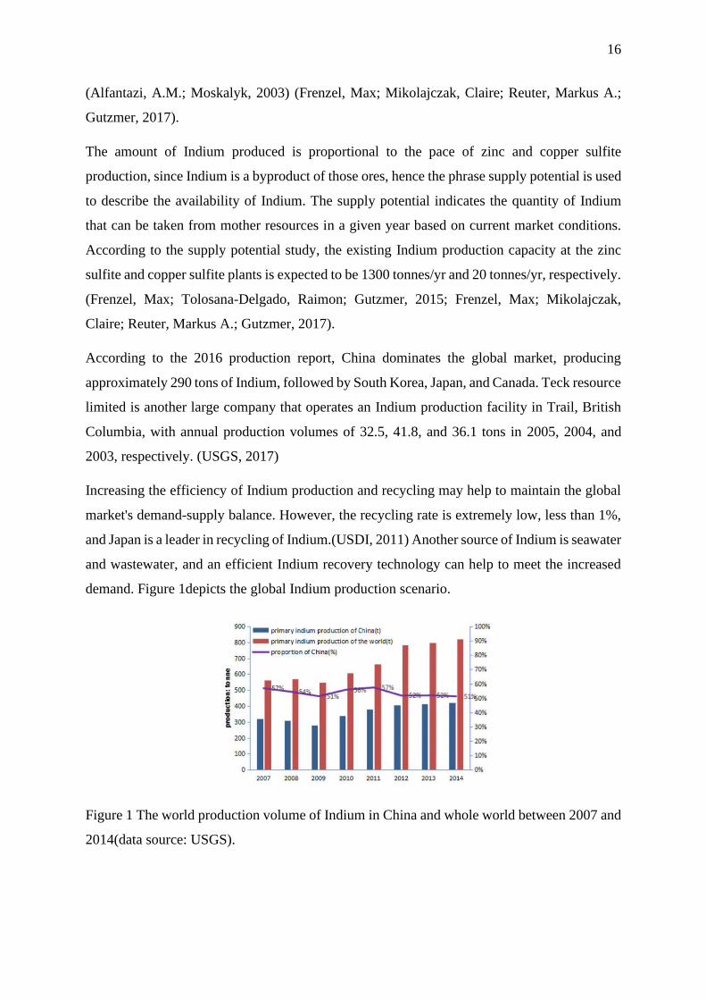
Increasing the efficiency of Indium production and recycling may help to maintain the global
market's demand-supply balance. However, the recycling rate is extremely low, less than 1%,
and Japan is a leader in recycling of Indium.(USDI, 2011) Another source of Indium is seawater
and wastewater, and an efficient Indium recovery technology can help to meet the increased
demand. Figure 1depicts the global Indium production scenario.
Figure 1 The world production volume of Indium in China and whole world between 2007 and
2014(data source: USGS).
17
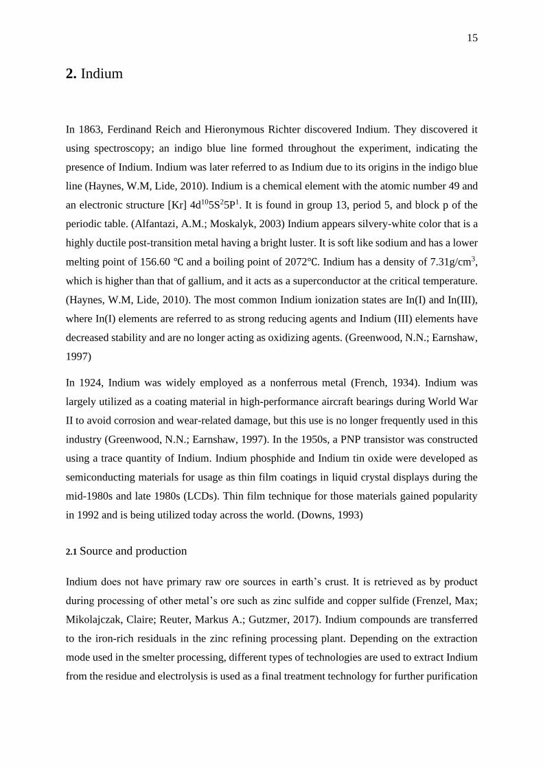
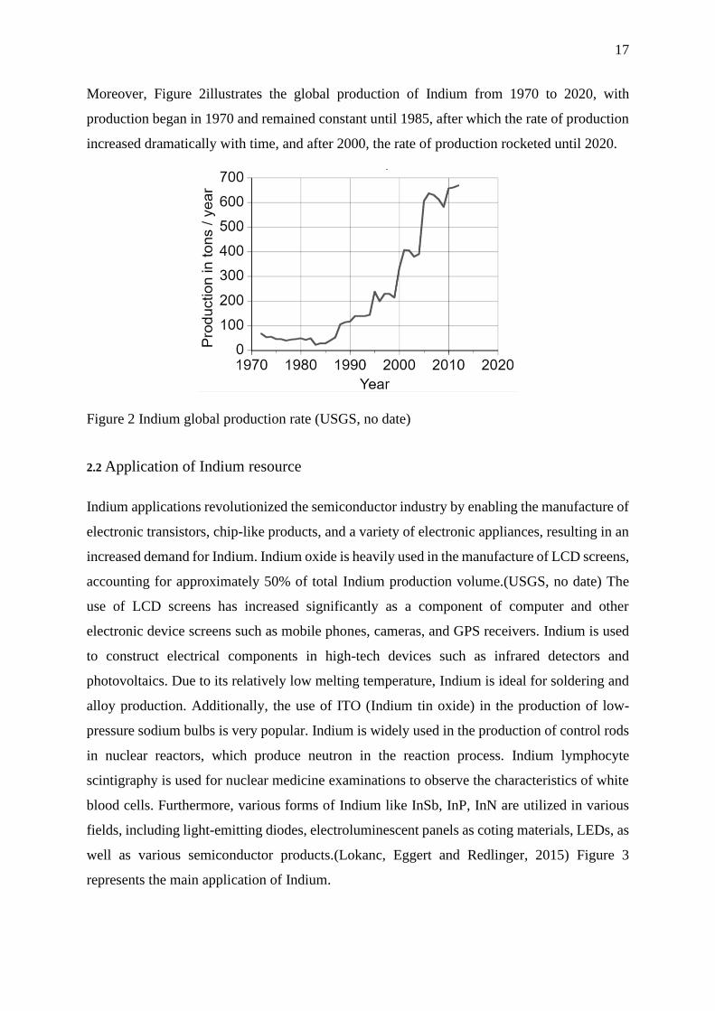
Moreover, Figure 2illustrates the global production of Indium from 1970 to 2020, with
production began in 1970 and remained constant until 1985, after which the rate of production
increased dramatically with time, and after 2000, the rate of production rocketed until 2020.
Figure 2 Indium global production rate (USGS, no date)
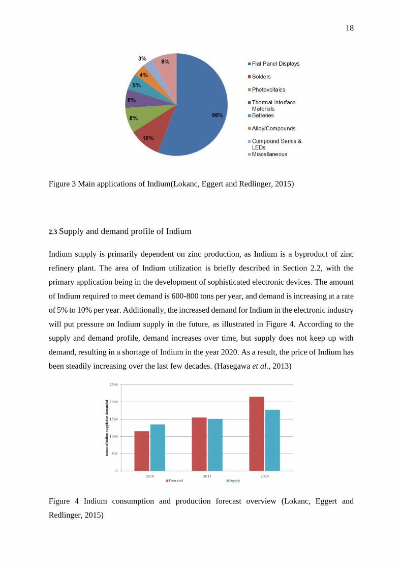
2.2 Application of Indium resource
Indium applications revolutionized the semiconductor industry by enabling the manufacture of
electronic transistors, chip-like products, and a variety of electronic appliances, resulting in an
increased demand for Indium. Indium oxide is heavily used in the manufacture of LCD screens,
accounting for approximately 50% of total Indium production volume.(USGS, no date) The
use of LCD screens has increased significantly as a component of computer and other
electronic device screens such as mobile phones, cameras, and GPS receivers. Indium is used
to construct electrical components in high-tech devices such as infrared detectors and
photovoltaics. Due to its relatively low melting temperature, Indium is ideal for soldering and
alloy production. Additionally, the use of ITO (Indium tin oxide) in the production of low-
pressure sodium bulbs is very popular. Indium is widely used in the production of control rods
in nuclear reactors, which produce neutron in the reaction process. Indium lymphocyte
scintigraphy is used for nuclear medicine examinations to observe the characteristics of white
blood cells. Furthermore, various forms of Indium like InSb, InP, InN are utilized in various
fields, including light-emitting diodes, electroluminescent panels as coting materials, LEDs, as
well as various semiconductor products.(Lokanc, Eggert and Redlinger, 2015) Figure 3
represents the main application of Indium.
18
Figure 3 Main applications of Indium(Lokanc, Eggert and Redlinger, 2015)
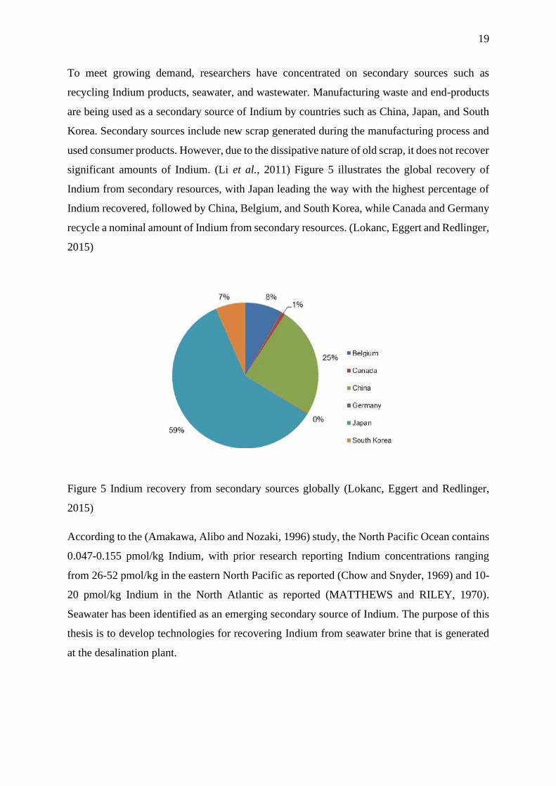
2.3 Supply and demand profile of Indium
Indium supply is primarily dependent on zinc production, as Indium is a byproduct of zinc
refinery plant. The area of Indium utilization is briefly described in Section 2.2, with the
primary application being in the development of sophisticated electronic devices. The amount
of Indium required to meet demand is 600-800 tons per year, and demand is increasing at a rate
of 5% to 10% per year. Additionally, the increased demand for Indium in the electronic industry
will put pressure on Indium supply in the future, as illustrated in Figure 4. According to the
supply and demand profile, demand increases over time, but supply does not keep up with
demand, resulting in a shortage of Indium in the year 2020. As a result, the price of Indium has
been steadily increasing over the last few decades. (Hasegawa et al., 2013)
Figure 4 Indium consumption and production forecast overview (Lokanc, Eggert and
Redlinger, 2015)
19
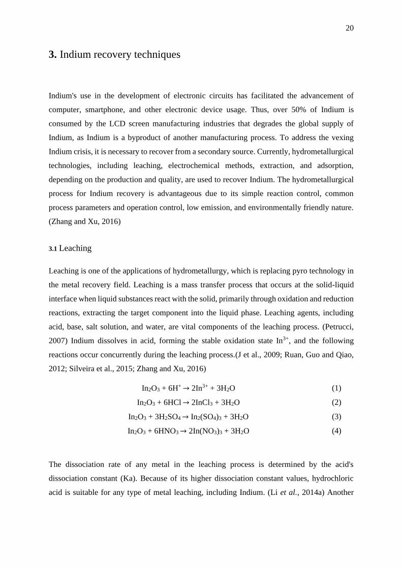
To meet growing demand, researchers have concentrated on secondary sources such as
recycling Indium products, seawater, and wastewater. Manufacturing waste and end-products
are being used as a secondary source of Indium by countries such as China, Japan, and South
Korea. Secondary sources include new scrap generated during the manufacturing process and
used consumer products. However, due to the dissipative nature of old scrap, it does not recover
significant amounts of Indium. (Li et al., 2011) Figure 5 illustrates the global recovery of
Indium from secondary resources, with Japan leading the way with the highest percentage of
Indium recovered, followed by China, Belgium, and South Korea, while Canada and Germany
recycle a nominal amount of Indium from secondary resources. (Lokanc, Eggert and Redlinger,
2015)
Figure 5 Indium recovery from secondary sources globally (Lokanc, Eggert and Redlinger,
2015)
According to the (Amakawa, Alibo and Nozaki, 1996) study, the North Pacific Ocean contains
0.047-0.155 pmol/kg Indium, with prior research reporting Indium concentrations ranging
from 26-52 pmol/kg in the eastern North Pacific as reported (Chow and Snyder, 1969) and 10-
20 pmol/kg Indium in the North Atlantic as reported (MATTHEWS and RILEY, 1970).
Seawater has been identified as an emerging secondary source of Indium. The purpose of this
thesis is to develop technologies for recovering Indium from seawater brine that is generated
at the desalination plant.
20
3. Indium recovery techniques
Indium's use in the development of electronic circuits has facilitated the advancement of
computer, smartphone, and other electronic device usage. Thus, over 50% of Indium is
consumed by the LCD screen manufacturing industries that degrades the global supply of
Indium, as Indium is a byproduct of another manufacturing process. To address the vexing
Indium crisis, it is necessary to recover from a secondary source. Currently, hydrometallurgical
technologies, including leaching, electrochemical methods, extraction, and adsorption,
depending on the production and quality, are used to recover Indium. The hydrometallurgical
process for Indium recovery is advantageous due to its simple reaction control, common
process parameters and operation control, low emission, and environmentally friendly nature.
(Zhang and Xu, 2016)
3.1 Leaching
Leaching is one of the applications of hydrometallurgy, which is replacing pyro technology in
the metal recovery field. Leaching is a mass transfer process that occurs at the solid-liquid
interface when liquid substances react with the solid, primarily through oxidation and reduction
reactions, extracting the target component into the liquid phase. Leaching agents, including
acid, base, salt solution, and water, are vital components of the leaching process. (Petrucci,
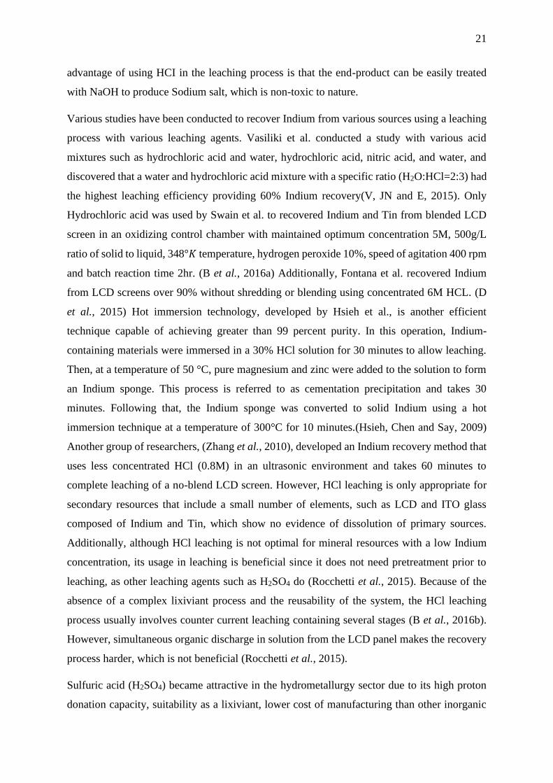
2007) Indium dissolves in acid, forming the stable oxidation state In3+, and the following
reactions occur concurrently during the leaching process.(J et al., 2009; Ruan, Guo and Qiao,
2012; Silveira et al., 2015; Zhang and Xu, 2016)
In2O3 + 6H+ → 2In3+ + 3H2O (1)
In2O3 + 6HCl → 2InCl3 + 3H2O (2)
In2O3 + 3H2SO4 → In2(SO4)3 + 3H2O (3)
In2O3 + 6HNO3 → 2In(NO3)3 + 3H2O (4)
The dissociation rate of any metal in the leaching process is determined by the acid's
dissociation constant (Ka). Because of its higher dissociation constant values, hydrochloric
acid is suitable for any type of metal leaching, including Indium. (Li et al., 2014a) Another
21
advantage of using HCI in the leaching process is that the end-product can be easily treated
with NaOH to produce Sodium salt, which is non-toxic to nature.
Various studies have been conducted to recover Indium from various sources using a leaching
process with various leaching agents. Vasiliki et al. conducted a study with various acid
mixtures such as hydrochloric acid and water, hydrochloric acid, nitric acid, and water, and
discovered that a water and hydrochloric acid mixture with a specific ratio (H2O:HCl=2:3) had
the highest leaching efficiency providing 60% Indium recovery(V, JN and E, 2015). Only
Hydrochloric acid was used by Swain et al. to recovered Indium and Tin from blended LCD
screen in an oxidizing control chamber with maintained optimum concentration 5M, 500g/L
ratio of solid to liquid, 348°𝐾 temperature, hydrogen peroxide 10%, speed of agitation 400 rpm
and batch reaction time 2hr. (B et al., 2016a) Additionally, Fontana et al. recovered Indium
from LCD screens over 90% without shredding or blending using concentrated 6M HCL. (D
et al., 2015) Hot immersion technology, developed by Hsieh et al., is another efficient
technique capable of achieving greater than 99 percent purity. In this operation, Indium-
containing materials were immersed in a 30% HCl solution for 30 minutes to allow leaching.
Then, at a temperature of 50 °C, pure magnesium and zinc were added to the solution to form
an Indium sponge. This process is referred to as cementation precipitation and takes 30
minutes. Following that, the Indium sponge was converted to solid Indium using a hot
immersion technique at a temperature of 300°C for 10 minutes.(Hsieh, Chen and Say, 2009)
Another group of researchers, (Zhang et al., 2010), developed an Indium recovery method that
uses less concentrated HCl (0.8M) in an ultrasonic environment and takes 60 minutes to
complete leaching of a no-blend LCD screen. However, HCl leaching is only appropriate for
secondary resources that include a small number of elements, such as LCD and ITO glass
composed of Indium and Tin, which show no evidence of dissolution of primary sources.
Additionally, although HCl leaching is not optimal for mineral resources with a low Indium
concentration, its usage in leaching is beneficial since it does not need pretreatment prior to
leaching, as other leaching agents such as H2SO4 do (Rocchetti et al., 2015). Because of the
absence of a complex lixiviant process and the reusability of the system, the HCl leaching
process usually involves counter current leaching containing several stages (B et al., 2016b).
However, simultaneous organic discharge in solution from the LCD panel makes the recovery
process harder, which is not beneficial (Rocchetti et al., 2015).
Sulfuric acid (H2SO4) became attractive in the hydrometallurgy sector due to its high proton
donation capacity, suitability as a lixiviant, lower cost of manufacturing than other inorganic
22
acids, and ability to produce an ecologically acceptable end-product. Filippou and Demopoulos
reported a skeletal reaction of Indium containing zinc ferrite and H2SO4 shown in eq (Filippou
and Demopoulos, 1997).
2ZnFe(2-x)InxO4 + 8 H2SO4 (aq) → 2ZnSO4(aq) + (2-x)Fe2 (SO4)3(aq) + xIn2(SO4)3 + 8H2O
The most often used method of dissolving metals in leaching is roasting with sulfuric acid at a
higher temperature. Guocai et al. obtained more than 90% Indium from contained slag using
an optimized system that included a controlled solid liquid ratio of 10%, a reaction duration of
1 h at 250 °C for roasting, a controlled solid liquid ratio of 10%, and a reaction time of 1 h at
60 °C for leaching (ZHU et al., 2007).
Rocchetti et al. investigated a pathway for Indium recovery from LCDs using cross current
leaching and the cementation technique. They used 2M H2SO4 to create an acidic environment
and maintained an 80°C temperature for 10 minutes for ten sequential leaching operations
followed by the cementation of sponge Indium recovery, which reduced greenhouse gas
emissions. The ten-step leaching method significantly increases profit margins compared to the
traditional one-step technique. (Rocchetti et al., 2015)
3.2 Pressure leaching
Pressure leaching is a kind of leaching in which soluble minerals or concentrates are chemically
dissolved under high pressure in order to extract the desired mineral from ores. Typically, this
process is performed in closed autoclaves. Indium recovery is linked with zinc ferrite, which
is found as a sulfide form in sphalerite, but the oxidation rate of sulfide is extremely slow under
atmospheric oxygen pressure. (Crundwell, 1988) Pressure leaching is a method for dealing with
the sluggish dissolving of In, Zn, and Fe. Li et al. performed a study for Indium and zinc
recovery utilizing pressure leaching technique, obtaining 99 percent zinc and more than 90
percent Indium from sphalerite. The whole experiment was carried out in closed autoclaves in
the presence of sulfuric acid and oxygen. To achieve maximum recovery, the process was
optimized with particular particle size 48𝜇𝑚, 1600 kPa oxygen partial pressure, 140 g/L
sulfuric acid concentration, temperature of 160°C, and 150-minute operating time. (C. Li et al.,
2010) In another research, Indium was dissolved by pressure leaching from zinc oxide flue dust
using sulfuric acid as a medium (X.-H. Li et al., 2010).
23
A demonstration was carried out to determine the impact of oxygen pressure on the Indium
leaching process, with the goal of increasing the oxidation rate in the leaching process. KMnO4
(2.5 percent) and H2O2 (0.5mL/g) were employed in a sulfuric acid (5.1 M) environment with
a temperature of 90 °C and a reaction time control of up to 150 minutes to complete the leaching
process and recover 90 percent of the Indium. Another research of leaching without oxygen
pressure and without oxidizing agent achieved 77% Indium recovery, proving that oxygen
pressure is not much advantageous for the Indium leaching process. (Pradhan, Panda and Sukla,
2017)
3.3 Extraction
In hydrometallurgy, extraction is referred to as solvent extraction, which is a more extensive
kind of leaching for a few minerals processing. Due to the simplicity of the equipment design,
the solvent's recyclability, and controlled process parameters, this method makes recovery
feasible. Numerous studies have shown the solvent extraction process's viability for Indium
recovery (Paiva, 2006) and Cyanex 923, bis-2, 2-ethylhexylphosphonic mono-2-ethylhexyl
ester, and tributyl phosphate are the most often used extractants for Indium recovery.
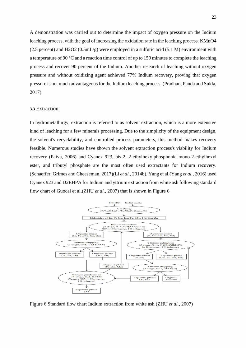
(Schaeffer, Grimes and Cheeseman, 2017)(Li et al., 2014b). Yang et al.(Yang et al., 2016) used
Cyanex 923 and D2EHPA for Indium and yttrium extraction from white ash following standard
flow chart of Guocai et al.(ZHU et al., 2007) that is shown in Figure 6
Figure 6 Standard flow chart Indium extraction from white ash (ZHU et al., 2007)
24
In 2013, the same author investigated Indium selective solvents containing Cyanex 923,
Cyanex 272, D2EHPA, and TBP. He discovered that diluted D2EHPA in kerosene provides
high selectivity for Indium separation, exceeding 99 percent. Meanwhile, three solvent systems
were investigated, including TBP, D2EHPA, and a mixture of the two, to recover Indium and
Tin from LCD wastes. The mixture of TBP (0.8-1M) and D2EHPA (0.2M) separated Indium
selectively from solution, whereas only the D2EHPA solution separated Indium and Tin
simultaneously from solution.(Yang, Retegan and Ekberg, 2013) However, another research
group showed that utilizing HCl stripping, Indium can be separated from the loaded
D2EHPA.(Virolainen, Ibana and Paatero, 2011) Ruan et al. conducted a similar experiment
utilizing three steps of processing with 97 percent separation, beginning with H2SO4 leaching,
followed by D2EHPA extraction and lastly Indium recovery by HCl stripping. (Ruan, Guo and
Qiao, 2012). (Chang et al., 2016) demonstrated on a laboratory scale the separation of iron and
Indium utilizing D2EHPA extractant from sulphate leach solution employing a steam rotating
packed bed contractor and investigated effect of various parameters for instance extractant
concentration, pH of initial solution, concentration of initial iron, ratio of flow rate and effect
of gravity on the separation. Approximately 99% recovery was obtained using the following
optimum parameters: 0.3 mol/L acid solution in feed, Aquas and organic flow ratio 2, organic
phase flow rate of 30L/h, high gravity factor of about 83, extractant D2EHPA 25% vol in
kerosene, 7g/L initial iron concentration, and 3mol/L HCl solution. Another research was
performed in which Indium extracted using D2EHPA was recycled and utilized in a
manufacturing facility through precipitation and calcination. (Chang et al., 2016) Several
studies have shown that D2EHPA extractant is superior for selective separation of Indium from
various solutions using HCl as a stripping agent (Zhang et al., 2017). Furthermore, Fontana et
al. used polyethylene glycol to form a biphasic phase that yielded 80-95 percent Indium in the
bottom extraction phase and 5-20 percent Indium in the top extraction phase (D et al., 2015).
Zonyl FSA was formed metal 1, 10-phenanthroline chelates complex during extraction and
obtained 96.7% recovery of Indium (Kato et al., 2013).
3.4 Electrolysis
Electrolysis is a method for separating desired products on the cathode or anode surface.
Grimes demonstrated in 2017 the separation of Indium from Indium tin-lead-based compounds
using electrolysis methods and leaching agents such as acetic and perchloric acid. In this work,
a new cylindrical mesh electrode with three consecutive separation stages was utilized. Lead
25
was removed initially from the solution without the addition of the complexing reagent SCN-,
resulting in a recovery of 97 % of lead at a maximum concentration of 2 mg/L after an eight-
hour reaction. The solution produced in the first stage is passed to the second step operation,
which includes the addition of 0.02 mol/L complexing reagent SCN- to aid in the multistep
electrolysis process. The electrolysis procedure was performed for eight hours and recovered
94% of the tin at a concentration of 3mg/L. Finally, Indium was recovered as oxyhydroxide on
the anode area and the concentration of SCN- was increased to 1 mol/L to enable electrolysis.
This electrolysis procedure took 24 hours and recovered 98% of the Indium (Grimes, Yasri and
Chaudhary, 2017). Another study was conducted for Indium recovery from e -waste by
utilizing HCl leaching process and extraction by PC88A extractant. To obtain maximum purity
of Indium, electrolytic separating was used after extraction and 99.99% pure Indium was
obtained. (Grimes, Yasri and Chaudhary, 2017)
3.5 Cementation and precipitation
Indium content is present in lead smelting dust in solid form; however, separation of Indium
from dust is challenging owing to the existence of lead content in the dust; thus, lead content
must be eliminated prior to leaching in order to extract Indium from lead dust. Sawai et al.
developed a three-step processing method for recovering Indium from lead smelting dust. In
the first stage, lead was separated using chelant aided washing with ethylene diamine
disuccinate, which possesses selectivity for lead. For the leaching procedure, a solution of HCl
and H2SO4 was employed, and dissolved Indium was recovered selectively by precipitation at
pH 5, resulting in 88% recovery of Indium. (Sawai et al., 2015). (Jiang, Liang and Zhong,
2011) conducted another research for Indium recovery from lead ore in which Na5P3O10 was
used to precipitate Indium in a pressured oxidation system. Under optimal conditions, the
method demonstrated efficiency with 95 percent Indium recovery: molar ratio of Na5P3O10 and
Indium was 0.91, pH 2.6, and reaction time 1.5 hours. The precipitation produced as
NaIn3(P3O10)2 crystals, which was verified by XRD analysis, was then collected for further
treatment, which started with dissolving the precipitate with H2SO4 for extraction. Later, at
room temperature and pH 3.0, ZnO powder was added into the solution, which was maintained
for 7 hours to complete the cementation process, yielding 97% pure Indium recovery. Another
study utilized ammonia instead of Na5P3O10 in a similar consecutive procedure that included
precipitation, leaching, extraction, and cementation and 92% Indium recuperation from the 145
ppm Indium zinc plant waste was accomplished (Jiang, Liang and Zhong, 2011).
26
It is more appropriate to recover Indium from ITO wastes through an acid leaching and
cementation process. However, the presence of tin in the leaching solution acts as a barrier to
the cementation process, since it must be removed from the solution prior to the cementation
process, which is a challenging procedure. (Li et al., 2011) overcame the obstacle by
introducing a sulfide precipitation into the process under optimal conditions, which included a
101.3Kpa H2S partial pressure, a 100g/L H2SO4 concentration, a temperature of 60°C, and a
precipitation duration of 10 minutes. Following that, zinc was added to aid in the development
of the cementation sponge. Zinc concentration and cementation duration both have an impact
on the purity of Indium. According to (Rocchetti, Amato and Beolchini, 2016) zinc
concentration and duration are directly linked to cementation efficiency; as zinc concentration
increases, Indium purity decreases, while increasing the time of the cementation process
increases Indium purity.
3.6 Extraction using sub-critical water
Solvent extraction is used to aid Indium recovery during the leaching process in order to get
pure Indium from the leaching solution. Separation of extractant solution after post treatment
is challenging and requires additional recycling facilities, which is not ecologically favorable.
Sub-critical water is an environmentally friendly technology that may be an ideal option for
hydrometallurgical solvent extraction processes since it may overcome prior solvent extraction
process limitations. Water characteristics vary as the temperature rises; the boiling point of
water is 100 °C, and the critical point is 374 °C, at which significant pressure is required to
maintain the liquid condition of the water, referred to as sub critical water. Water in the
subcritical state decreases the dielectric constant, resulting in improved solubility for
hydrophobic materials. Additionally, subcritical water increases the value of the ionic product
by thrice at 250 °C compared to ambient temperature.(Tavakoli and Yoshida, 2006) Sub-
critical water has been used in several works to recover different products from wastes such as
amino acid, fatty acid, organic acid and nutrients (H, M and Y, 1999; Tavakoli and Yoshida*,
2005). Using sub-critical water and a five-minute reaction period, Indium was recovered from
color filters and thin-film transistors at rates of more than 83% and 7%, respectively. The major
benefit of this method was that Indium was separated from waste as Indium oxide in solid form,
which can be readily separated from liquid solution, and the separation efficiency is influenced
by sub-critical water temperature.(Yoshida et al., 2014) investigated the impact of various basic
chemicals present in separation systems, such as potassium hydroxide, sodium hydroxide,
27
ammonia, sodium carbonate, calcium hydroxide, and diethyl amin, as well as their
concentration, on Indium recovery. With the same reaction time and temperature at 160°C, 0.1
N NaOH recovered over 95% of the Indium from TFT glass and 99% from color filter glass
(Yoshida et al., 2015). While the method offers several advantages for Indium recovery, it
requires a significant amount of energy and money to construct the infrastructure necessary to
maintain high pressure.
3.7 Extraction by supercritical fluid
Supercritical fluid extraction is superior to conventional fluid extraction because it is a green
technology that achieves higher separation rates and efficiencies while using nontoxic, low-
cost, and nonflammable liquefied CO2. Additionally, it is more eco-friendly than traditional
fluid extraction.(Ghoreishi, Ansari and Ghaziaskar, 2012) CO2-based supercritical fluids reach
supercritical phase at or above the critical temperature (31.1°C) and pressure (7.38MPa) with
the same density as liquid CO2. Viscosity is reduced compared to CO2 and high solubility
capacities are observed due to huge diffusion capabilities, lower viscosity, and zero surface
tension.(Ghoreishi, Ansari and Ghaziaskar, 2012) A study discovered that supercritical fluid
extracts Indium (76.5%) directly from ITO and cellphones using co-solvents such as citric acid
and malic acid at ambient pressure and that the process took 180 minutes to complete. While
only supercritical CO2 achieves remarkable separation (94.6 percent recovery) in a short period
of time and without the use of a co-solvent (30 min).(Argenta et al., 2017)
3.8 Adsorption
The Indium recovery technologies discussed previously have limitations in several areas,
including the fact that leaching is not always sufficient for Indium recovery; additional
technologies such as solvent extraction, precipitation, electrolysis, and cementation are
required to recover Indium from leaching solutions. Following processing, leaching and
solvent extraction produce a large quantity of hazardous chemicals that drain into the
environment, which is not environmentally friendly. Those processes take much more time
than the production volume and product quality in terms of purity. In terms of mechanism and
process control, the process is complicated and difficult to comprehend. In contrast, the
adsorption method for Indium recovery is most flexible in terms of selectivity, simplicity and
environmental friendliness.
28
Several adsorption studies were carried out utilizing commercial resin for Indium recovery to
reveal adsorption properties and determine operating parameters in a thorough way (Jeon, Cha
and Choi, 2015). Due to its selectivity, ease of functionalization, and ease of extraction of
Indium from adsorbent, ion exchange resins became an appealing subject for Indium recovery.
Iminodiacetic acid-based resin is commonly utilized in the manufacture of a variety of
commercial resins, including Amberlite IRC748, Lewatit TP-260, and Lewatit TP-207. Fortes
et al. investigated the capture of Indium on the commercial resin Amberlite IRC748 using
dynamic adsorption and obtained 99.5% Indium recovery using H2SO4 elution at a flow rate of
5.0 mL/min (M. C. B. Fortes, Martins and Benedetto, 2007). Using iminodiacetic acid resin,
(XIONG and YAO, 2008a) investigated the impact of various parameters on Indium adsorption
and determined the parameter values for maximum adsorption of 235.5 mg/g at 25℃
temperature and pH 4.52. (Yuchi et al., 1992) did another investigation to evaluate the
adsorption equilibrium of various metal trivalent ions (M+) utilizing chelating resin
incorporating iminodiacetic acid. This study demonstrated the impact of anions and
iminodiacetic acid ratio on formation of metal ligand complex for adsorption and determined
the amount of iminodiacetic acid groups per unit weight. Few research has been made for metal
adsorption e.g. In, Eu, Cu, Co, Ga, Ni using chitosan which is natural modified polymeric
substants.
Assefi et al. investigated the recovery of Indium from waste LCD panels using three distinct
microporous ion exchange resins (Lewatit TP-208, Lewatit TP-260 and Amberlite IRA 743).
TP-208, for example, is made of iminodiacetic acid resin and has been demonstrated to be a
better ion exchange for Indium recovery. Indium recovery is dependent on a number of
variables, including pH, solute concentration, and temperature. In this investigation, pH values
ranging from 0.5 to 4 were used to determine Indium recovery. At lower pH values, such as
(pH 1-2), Indium ion generates hydronium ion, which acts as an inert towards adsorbent sites.
As pH values increase, Indium recovery increases until pH 4. Above pH 4, the Indium ion
generates In(OH)3, a phase that has difficulties adhering to the adsorbent surface. By eluding
Indium from resin with HCl acid, Indium was recovered. (Assefi et al., 2018a) Another study
was done on Indium recovery utilizing TP-207 to determine the Indium adsorption behavior
and revealed a 55mg/g adsorption capacity at pH 0.8 (Lee and Lee, 2016) and the technique
for recovering Indium from resin was identical to that described in a previously published work.
(Assefi et al., 2018a) Ferella et al. investigated the Indium recovery method using commercial
29
Amberlite IRA-748 and got the highest adsorption capacity at pH 3 with a 24hr contact period.
(F et al., 2017)
Due to the rarity of specific Indium adsorbent materials, numerous studies have been
undertaken on functionalizing resins for selective Indium adsorption. Chang et al. developed
chelate fiber resin for selective adsorption and obtained 95% recovery from a mixture of Sn,
Cr, Ti, and In at pH of 4-7 with a feed flow rate of 10mL/min. (X et al., 1993) (Yuan et al.,
2010) studied the coated solvent impregnated resin for selective Indium recovery and
determined that the optimal pH for Indium adsorption was 1.5. Additionally, (Li et al., 2012)
modified a coated solvent impregnated resin with a styrene-divinylbenzene copolymer
supported sec-octyl phenoxy acetic acid. This offered Indium selectivity at pH 3 across a wide
temperature range and was stable for three successive regenerations. The Indium adsorption
process was investigated using multiwalled carbon nanotubes, which had an adsorption
capacity of 40 mg/g. However, the disadvantage of this adsorbent was that it was not selective
when other metal ions were present in the solution. (Akama, Suzuki and Monobe, 2016)
Since the previous several decades, additive manufacturing has gained popularity for a variety
of applications, including industrial, water treatment, and environmental concerns. The use of
raw materials and the application of additive manufacturing technologies are increasing
dramatically as they are used in the emergence of new technologies with success and
application. This technique is associated with various instruments, which enables layer-by-
layer deposition to obtain the required mechanical and chemical qualities.
The technique requires less material, which lowers the cost of production. (Gibson, Rosen and
Stucker, 2010) Recently additive manufacturing technologies has been used for adsorption and
ion exchange membranes for selective metal recovery. Lahtinen et al. developed an additively
manufactured adsorbent for gold recovery using nylon-based materials. This results in a greater
recovery % because nylon 6.6 and nylon 12 have a stronger affinity for gold while AM-based
adsorbents have a larger surface area and mechanical stability, which increases the adsorbent's
reusability.(Lahtinen et al., 2019) Another study was made for selectively recover metal such
as Pd, Pt, Au from e-waste using 3D printed scavenger filter. A mixture of polypropylene and
anion exchanger resin was used to produce adsorbent that especially abled to capture Pd and
Pt from waste. (Lahtinen et al., 2018) This principle is used in this thesis work for
manufacturing 3D printed adsorbent for Indium recovery from sea water.
30
4. Adsorbent materials for Indium recovery
Numerous studies on Indium recovery have been conducted using a variety of adsorbent
materials, including ion exchange resins,(M. C. B. Fortes, Martins and Benedetto, 2007)
chelating cellulose,(Akama, Suzuki and Monobe, 2016) modified metosol reagent,(Timofeev
et al., 2017) chelating fiber, microbeads, and carbon nanotubes. Three distinct adsorbent
materials (Lewatit® TP-207, Lewatit® TP-260, and Amberlite® IRA-743) were used in this
thesis to produce additively manufactured adsorbents, and their effectiveness was evaluated
and compared. This section gives an overview of those materials.
4.1 Resin TP-207
Lewatit® TP-207 is a commercial cation exchange resin that is produced using an
iminodiacetic acid-based chelating agent. It is designed specifically for the adsorption of heavy
metals from solution. This is a mildly acidic material that is capable of functioning in weakly
acidic or basic solutions.
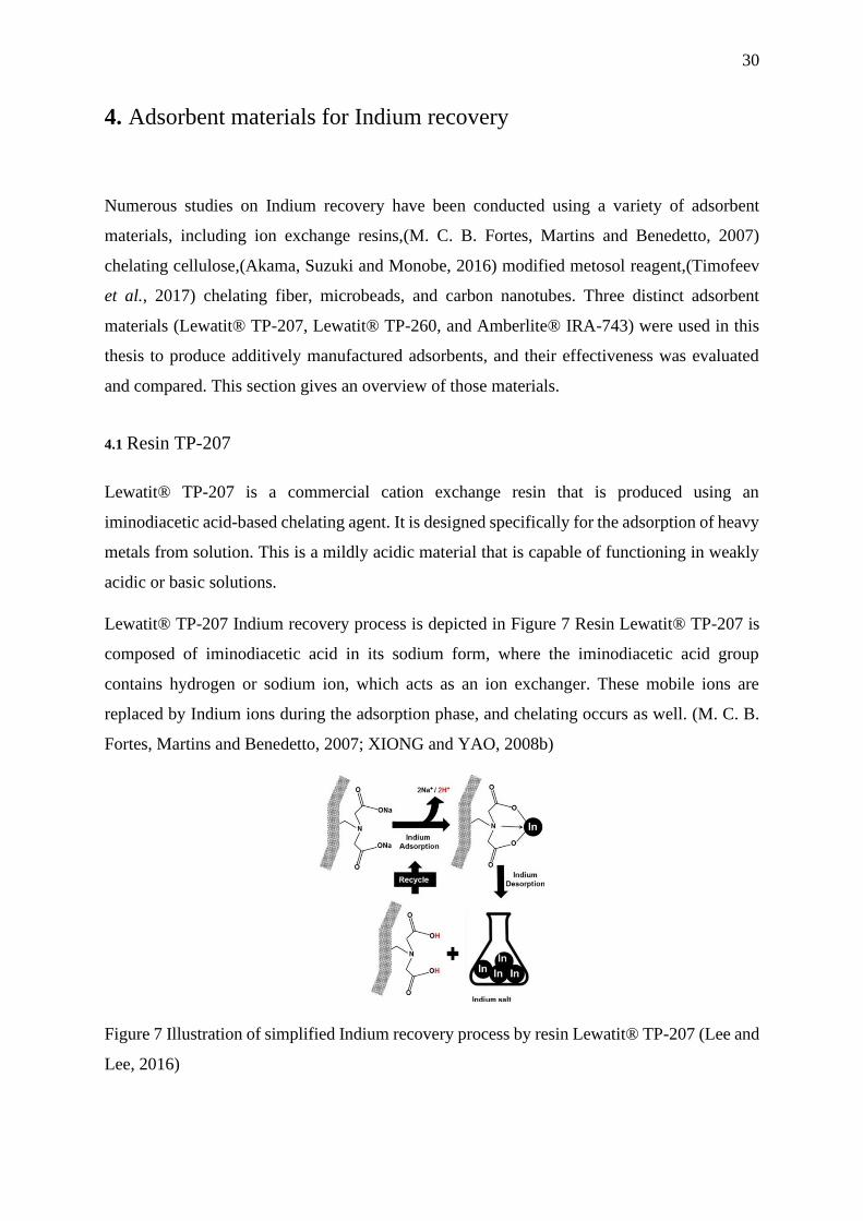
Lewatit® TP-207 Indium recovery process is depicted in Figure 7 Resin Lewatit® TP-207 is
composed of iminodiacetic acid in its sodium form, where the iminodiacetic acid group
contains hydrogen or sodium ion, which acts as an ion exchanger. These mobile ions are
replaced by Indium ions during the adsorption phase, and chelating occurs as well. (M. C. B.
Fortes, Martins and Benedetto, 2007; XIONG and YAO, 2008b)
Figure 7 Illustration of simplified Indium recovery process by resin Lewatit® TP-207 (Lee and
Lee, 2016)
31
After the adsorption process is complete, the adsorbent is filtered from the solution and the
resin is transferred to an acid solution for desorption. By introducing a hydrogen ion to the
resin, Indium can be removed. This hydrogen ion continues the adsorption process in the same
manner as the preceding adsorption phase. TP-207's Indium recovery procedure is extremely
easy and convenient in comparison to other approaches. The adsorption capacity of this resin
is dependent on few operational parameters, including pH, temperature, and the concentration
of various metal ions presence in solution.(Lee and Lee, 2016)
4.2 Resin Lewatiti® TP-260
Lewatiti® TP-260 is a cation exchange resin composed of an amino methyl phosphonic acid
group that demonstrates selectivity for heavy metals and is naturally mildly acidic. The resin
is microporous and contains disodium ions that attract metal ions from solution via ion
exchange and the production of chelates with the metal ion. (Lewatit-Lenntech, no date) A
study have established that phosphonic acid has an affinity for the Indium ion.(Assefi et al.,
2018a)
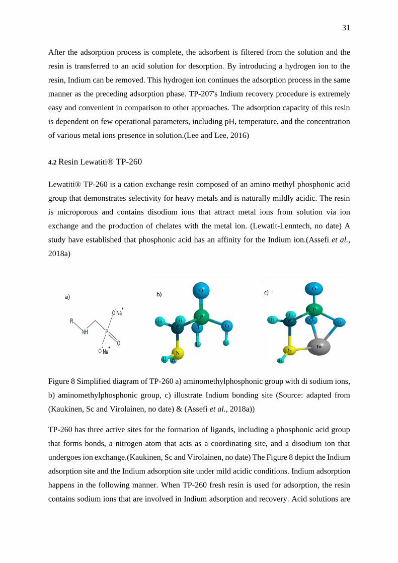
Figure 8 Simplified diagram of TP-260 a) aminomethylphosphonic group with di sodium ions,
b) aminomethylphosphonic group, c) illustrate Indium bonding site (Source: adapted from
(Kaukinen, Sc and Virolainen, no date) & (Assefi et al., 2018a))
TP-260 has three active sites for the formation of ligands, including a phosphonic acid group
that forms bonds, a nitrogen atom that acts as a coordinating site, and a disodium ion that
undergoes ion exchange.(Kaukinen, Sc and Virolainen, no date) The Figure 8 depict the Indium
adsorption site and the Indium adsorption site under mild acidic conditions. Indium adsorption
happens in the following manner. When TP-260 fresh resin is used for adsorption, the resin
contains sodium ions that are involved in Indium adsorption and recovery. Acid solutions are
32
often employed for Indium recovery and resin regeneration, with hydrogen ions occupying the
resin. Later, the hydrogen ion serves as an ion exchange site for the recovery of Indium.(Assefi
et al., 2018a) In this thesis, disodium-based TP-260 resin powder was utilized resin for additive
manufacturing.
4.3 Amberlite® IRA-743
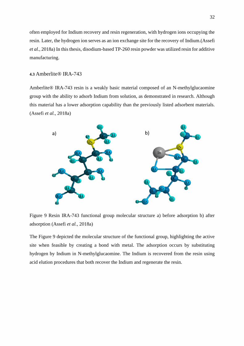
Amberlite® IRA-743 resin is a weakly basic material composed of an N-methylglucaomine
group with the ability to adsorb Indium from solution, as demonstrated in research. Although
this material has a lower adsorption capability than the previously listed adsorbent materials.
(Assefi et al., 2018a)
Figure 9 Resin IRA-743 functional group molecular structure a) before adsorption b) after
adsorption (Assefi et al., 2018a)
The Figure 9 depicted the molecular structure of the functional group, highlighting the active
site when feasible by creating a bond with metal. The adsorption occurs by substituting
hydrogen by Indium in N-methylglucaomine. The Indium is recovered from the resin using
acid elution procedures that both recover the Indium and regenerate the resin.
33
5. Additive Manufacturing
According to the Oxford definition, a process is a sequence of activities or steps taken to obtain
a desired outcome. Additive manufacturing (AM) is a set of operations that involve material
selection, material assembly methods, and the conversion of raw materials to three-dimensional
objects. Additive manufacturing works by layering and assembling to create the final
envisioned structure. A Computer Aided Design (CAD) program (or other similar software) is
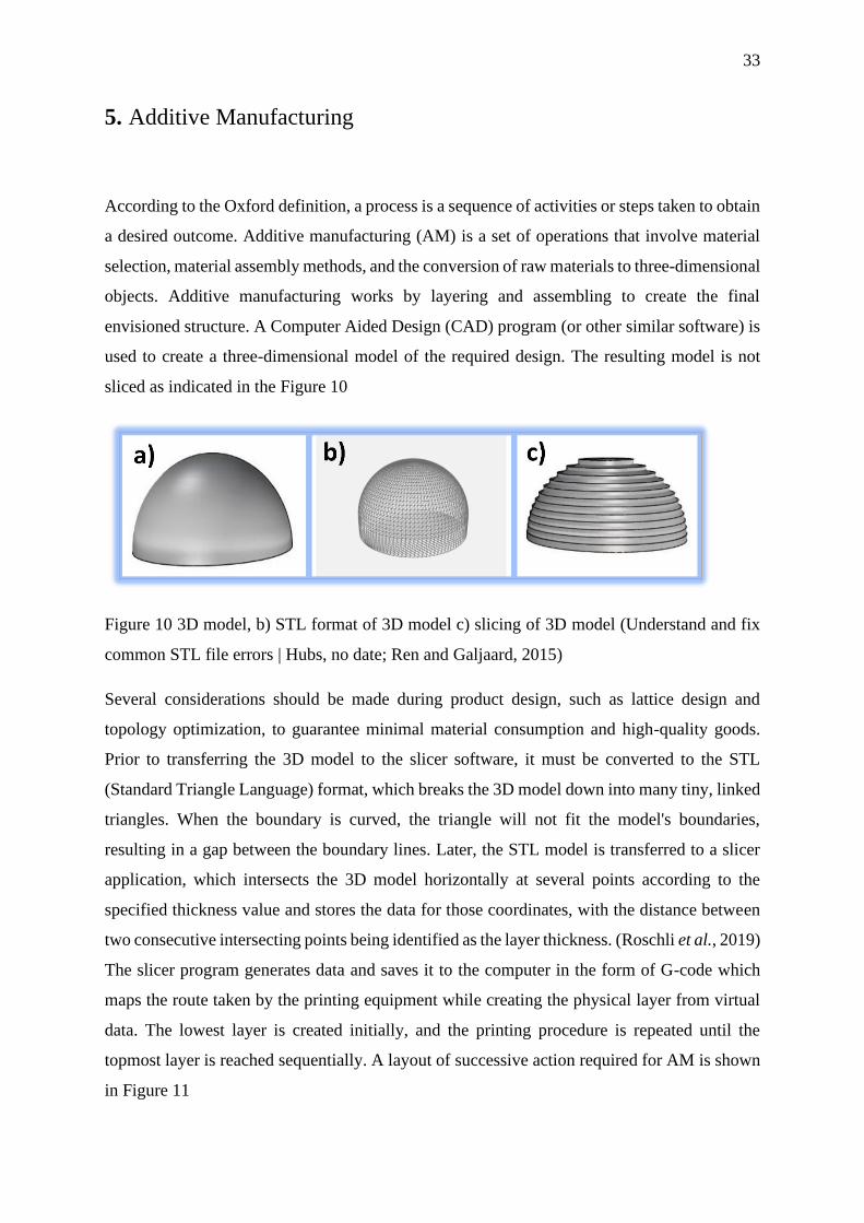
used to create a three-dimensional model of the required design. The resulting model is not
sliced as indicated in the Figure 10
Figure 10 3D model, b) STL format of 3D model c) slicing of 3D model (Understand and fix
common STL file errors | Hubs, no date; Ren and Galjaard, 2015)
Several considerations should be made during product design, such as lattice design and
topology optimization, to guarantee minimal material consumption and high-quality goods.
Prior to transferring the 3D model to the slicer software, it must be converted to the STL
(Standard Triangle Language) format, which breaks the 3D model down into many tiny, linked
triangles. When the boundary is curved, the triangle will not fit the model's boundaries,
resulting in a gap between the boundary lines. Later, the STL model is transferred to a slicer
application, which intersects the 3D model horizontally at several points according to the
specified thickness value and stores the data for those coordinates, with the distance between
two consecutive intersecting points being identified as the layer thickness. (Roschli et al., 2019)
The slicer program generates data and saves it to the computer in the form of G-code which
maps the route taken by the printing equipment while creating the physical layer from virtual
data. The lowest layer is created initially, and the printing procedure is repeated until the
topmost layer is reached sequentially. A layout of successive action required for AM is shown
in Figure 11
34
Figure 11 Steps of Additive Manufacturing (Kumar, 2020)
Every printing machine uses the same 3D CAD model and generated G code, but technologies
are divided into seven groups depending on how they operate, such as powder bed fusion,
binder jetting, Directed Energy Deposition, materials extrusion, materials jetting, sheet
lamination, and vat polymerization (Deckers, Vleugels and Kruth, 2014). The advantages of
additively manufactured adsorbents (3D printed adsorbents) are their mechanical stability and
optimized structure for the adsorption process. Separation of adsorbent following adsorption is
easier than conventional filtering, since it may be accomplished without the need of filter paper
or membrane.
5.1 Powder Bed Fusion (PBF)
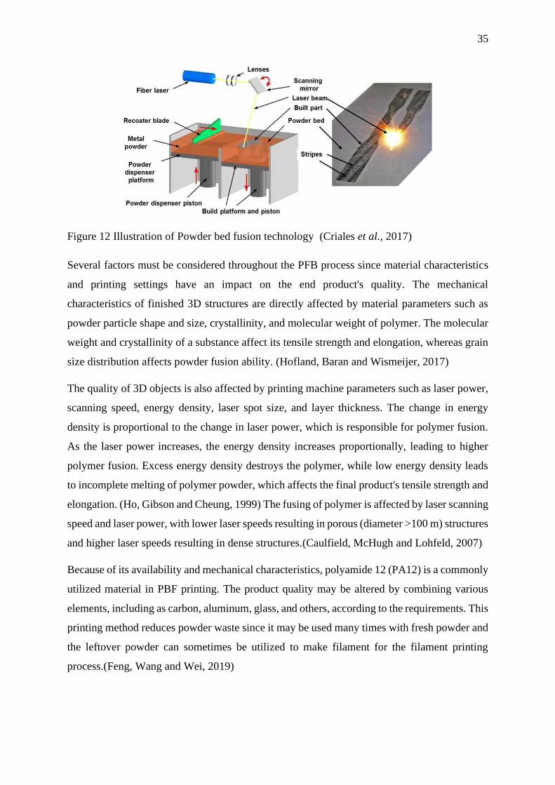
Powder bed fusion is a potential additive manufacturing technique for plastic materials, and it
may be used at any scale from small to large. The most typical components found in a PBF
printer are fiber lenses, scanning mirrors, laser beams, building platforms, powder dispenser
platforms, recoater blades, and pistons for powder dispense, as illustrated in Figure 12. The
PBF principle of operation is as follows: The printing process begins with preheating the
polymer powder near its melting point, then distributing the heated polymer powder evenly on
the building platform according to layer thickness with the help of a recoater blade that moves
from right to left. Afterwards, scanning with a CO2 laser beam on the construction platform
begins in order to sinter the polymer powder that forms the structure's single cross section layer.
After scanning each cross section of the building platform, move down one step according to
layer height and spread powder on the building platform as before, continuing until the object's
construction is complete. The scanner's scanning instructions and other commands, such as
layer thickness and structural coordination, are read from the G-code sent to the printer. 3D
objects must be ejected from the construction platform at the conclusion of the procedure, and
unsintered powder must be removed from the item. PBF technique does not need a supporting
framework since powder materials serve as the 3D object's supporting structure. The remaining
powder may be utilized for future printing projects, and fresh powder should be mixed with
old powder in a 1:1 ratio. (Ben Redwood and Filemon Schöffer, 2017)
35
Figure 12 Illustration of Powder bed fusion technology (Criales et al., 2017)
Several factors must be considered throughout the PFB process since material characteristics
and printing settings have an impact on the end product's quality. The mechanical
characteristics of finished 3D structures are directly affected by material parameters such as
powder particle shape and size, crystallinity, and molecular weight of polymer. The molecular
weight and crystallinity of a substance affect its tensile strength and elongation, whereas grain
size distribution affects powder fusion ability. (Hofland, Baran and Wismeijer, 2017)
The quality of 3D objects is also affected by printing machine parameters such as laser power,
scanning speed, energy density, laser spot size, and layer thickness. The change in energy
density is proportional to the change in laser power, which is responsible for polymer fusion.
As the laser power increases, the energy density increases proportionally, leading to higher
polymer fusion. Excess energy density destroys the polymer, while low energy density leads
to incomplete melting of polymer powder, which affects the final product's tensile strength and
elongation. (Ho, Gibson and Cheung, 1999) The fusing of polymer is affected by laser scanning
speed and laser power, with lower laser speeds resulting in porous (diameter >100 m) structures
and higher laser speeds resulting in dense structures.(Caulfield, McHugh and Lohfeld, 2007)
Because of its availability and mechanical characteristics, polyamide 12 (PA12) is a commonly
utilized material in PBF printing. The product quality may be altered by combining various
elements, including as carbon, aluminum, glass, and others, according to the requirements. This
printing method reduces powder waste since it may be used many times with fresh powder and
the leftover powder can sometimes be utilized to make filament for the filament printing
process.(Feng, Wang and Wei, 2019)
36
This printing technique was utilized to manufacture 3D adsorbent for metal recovery in this
thesis study. Various kinds of ion exchange resins were utilized in combination with polymers
such as PA12 and nylon to manufacture 3D adsorbents for Indium recovery.
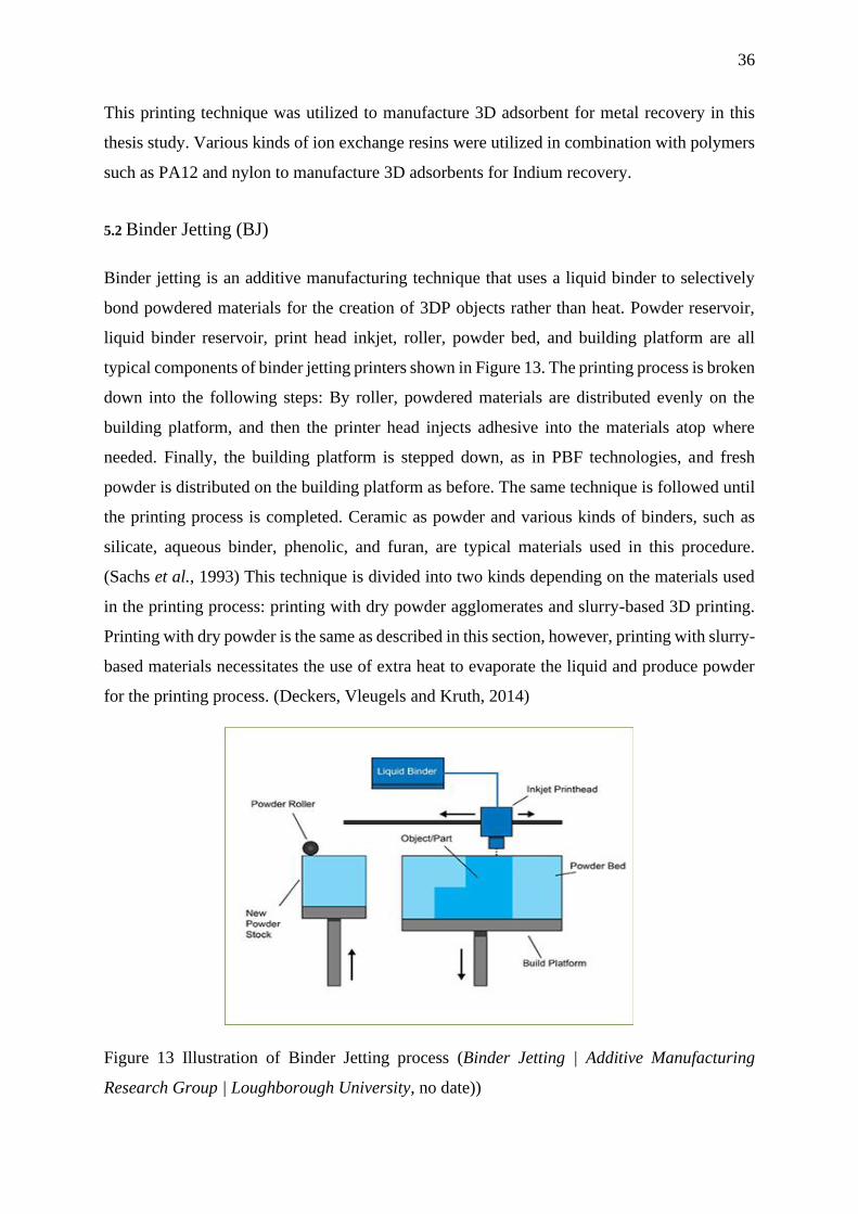
5.2 Binder Jetting (BJ)
Binder jetting is an additive manufacturing technique that uses a liquid binder to selectively
bond powdered materials for the creation of 3DP objects rather than heat. Powder reservoir,
liquid binder reservoir, print head inkjet, roller, powder bed, and building platform are all
typical components of binder jetting printers shown in Figure 13. The printing process is broken
down into the following steps: By roller, powdered materials are distributed evenly on the
building platform, and then the printer head injects adhesive into the materials atop where
needed. Finally, the building platform is stepped down, as in PBF technologies, and fresh
powder is distributed on the building platform as before. The same technique is followed until
the printing process is completed. Ceramic as powder and various kinds of binders, such as
silicate, aqueous binder, phenolic, and furan, are typical materials used in this procedure.
(Sachs et al., 1993) This technique is divided into two kinds depending on the materials used
in the printing process: printing with dry powder agglomerates and slurry-based 3D printing.
Printing with dry powder is the same as described in this section, however, printing with slurry-
based materials necessitates the use of extra heat to evaporate the liquid and produce powder
for the printing process. (Deckers, Vleugels and Kruth, 2014)
Figure 13 Illustration of Binder Jetting process (Binder Jetting | Additive Manufacturing
Research Group | Loughborough University, no date))
37
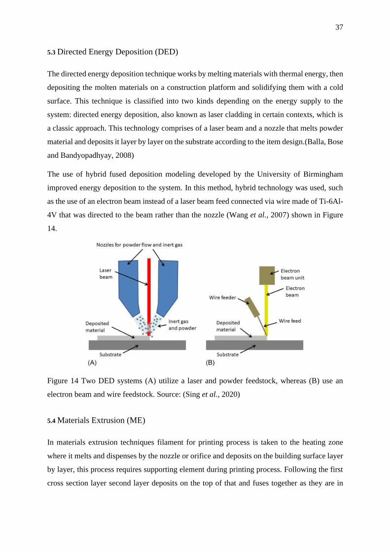
5.3 Directed Energy Deposition (DED)
The directed energy deposition technique works by melting materials with thermal energy, then
depositing the molten materials on a construction platform and solidifying them with a cold
surface. This technique is classified into two kinds depending on the energy supply to the
system: directed energy deposition, also known as laser cladding in certain contexts, which is
a classic approach. This technology comprises of a laser beam and a nozzle that melts powder
material and deposits it layer by layer on the substrate according to the item design.(Balla, Bose
and Bandyopadhyay, 2008)
The use of hybrid fused deposition modeling developed by the University of Birmingham
improved energy deposition to the system. In this method, hybrid technology was used, such
as the use of an electron beam instead of a laser beam feed connected via wire made of Ti-6Al-
4V that was directed to the beam rather than the nozzle (Wang et al., 2007) shown in Figure
14.
Figure 14 Two DED systems (A) utilize a laser and powder feedstock, whereas (B) use an
electron beam and wire feedstock. Source: (Sing et al., 2020)
5.4 Materials Extrusion (ME)
In materials extrusion techniques filament for printing process is taken to the heating zone
where it melts and dispenses by the nozzle or orifice and deposits on the building surface layer
by layer, this process requires supporting element during printing process. Following the first
cross section layer second layer deposits on the top of that and fuses together as they are in
38
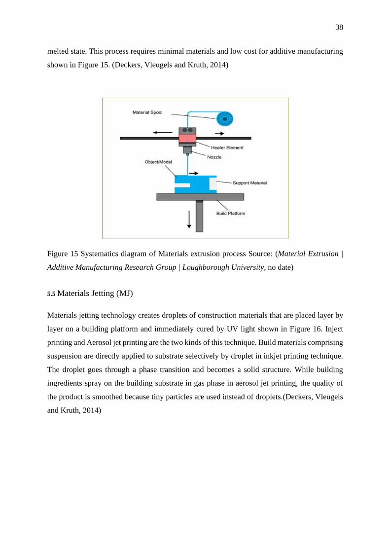
melted state. This process requires minimal materials and low cost for additive manufacturing
shown in Figure 15. (Deckers, Vleugels and Kruth, 2014)
Figure 15 Systematics diagram of Materials extrusion process Source: (Material Extrusion |
Additive Manufacturing Research Group | Loughborough University, no date)
5.5 Materials Jetting (MJ)
Materials jetting technology creates droplets of construction materials that are placed layer by
layer on a building platform and immediately cured by UV light shown in Figure 16. Inject
printing and Aerosol jet printing are the two kinds of this technique. Build materials comprising
suspension are directly applied to substrate selectively by droplet in inkjet printing technique.
The droplet goes through a phase transition and becomes a solid structure. While building
ingredients spray on the building substrate in gas phase in aerosol jet printing, the quality of
the product is smoothed because tiny particles are used instead of droplets.(Deckers, Vleugels
and Kruth, 2014)
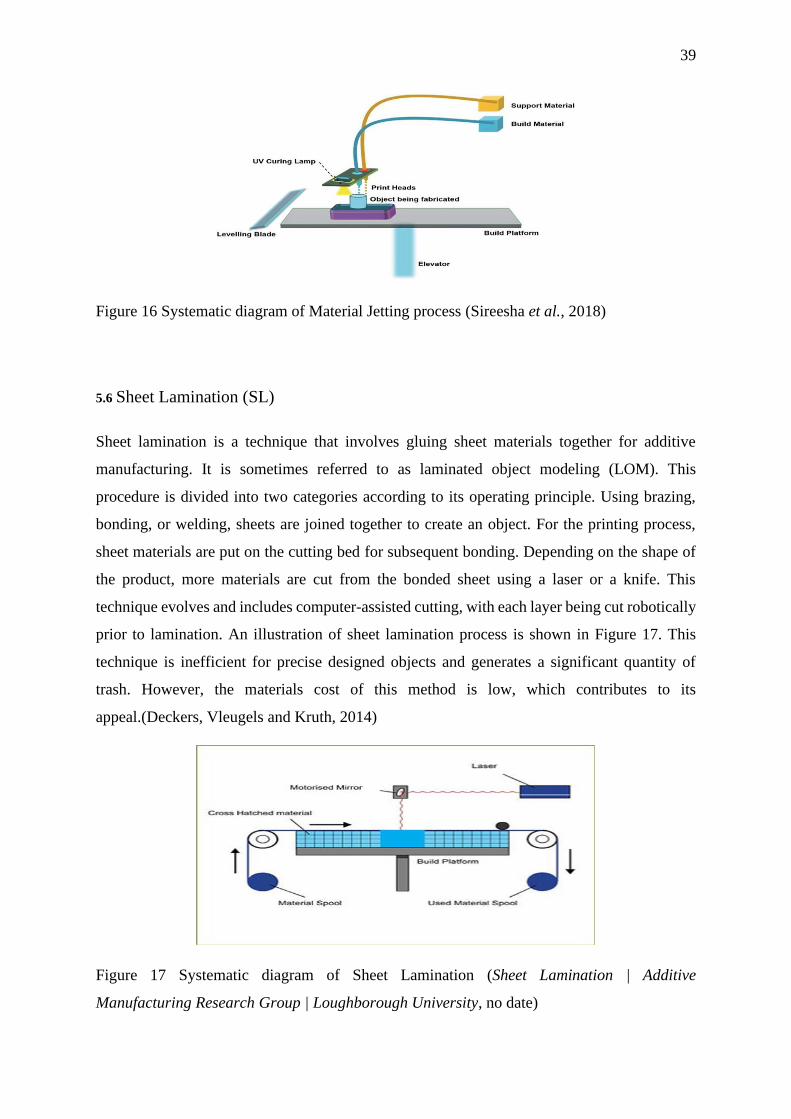
39
Figure 16 Systematic diagram of Material Jetting process (Sireesha et al., 2018)
5.6 Sheet Lamination (SL)
Sheet lamination is a technique that involves gluing sheet materials together for additive
manufacturing. It is sometimes referred to as laminated object modeling (LOM). This
procedure is divided into two categories according to its operating principle. Using brazing,
bonding, or welding, sheets are joined together to create an object. For the printing process,
sheet materials are put on the cutting bed for subsequent bonding. Depending on the shape of
the product, more materials are cut from the bonded sheet using a laser or a knife. This
technique evolves and includes computer-assisted cutting, with each layer being cut robotically
prior to lamination. An illustration of sheet lamination process is shown in Figure 17. This
technique is inefficient for precise designed objects and generates a significant quantity of
trash. However, the materials cost of this method is low, which contributes to its
appeal.(Deckers, Vleugels and Kruth, 2014)
Figure 17 Systematic diagram of Sheet Lamination (Sheet Lamination | Additive
Manufacturing Research Group | Loughborough University, no date)
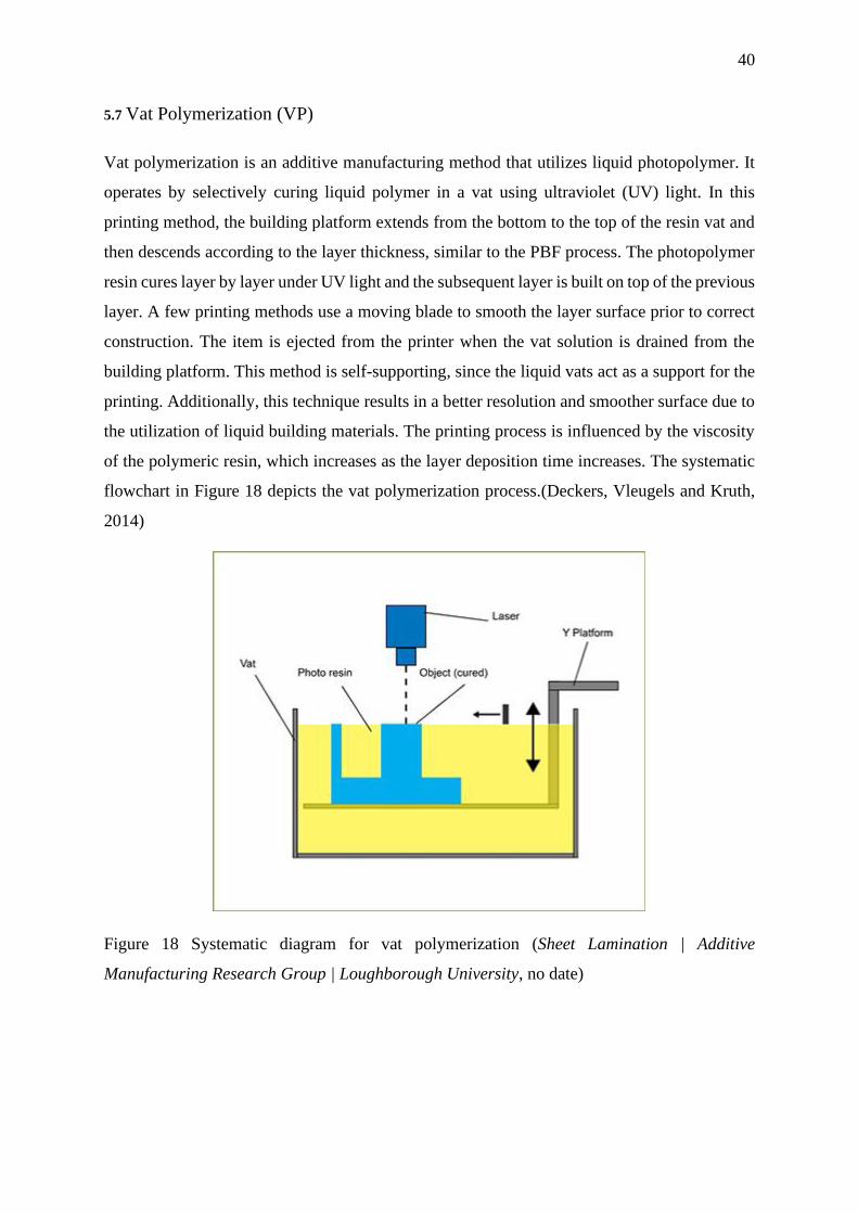
40
5.7 Vat Polymerization (VP)
Vat polymerization is an additive manufacturing method that utilizes liquid photopolymer. It
operates by selectively curing liquid polymer in a vat using ultraviolet (UV) light. In this
printing method, the building platform extends from the bottom to the top of the resin vat and
then descends according to the layer thickness, similar to the PBF process. The photopolymer
resin cures layer by layer under UV light and the subsequent layer is built on top of the previous
layer. A few printing methods use a moving blade to smooth the layer surface prior to correct
construction. The item is ejected from the printer when the vat solution is drained from the
building platform. This method is self-supporting, since the liquid vats act as a support for the
printing. Additionally, this technique results in a better resolution and smoother surface due to
the utilization of liquid building materials. The printing process is influenced by the viscosity
of the polymeric resin, which increases as the layer deposition time increases. The systematic
flowchart in Figure 18 depicts the vat polymerization process.(Deckers, Vleugels and Kruth,
2014)
Figure 18 Systematic diagram for vat polymerization (Sheet Lamination | Additive
Manufacturing Research Group | Loughborough University, no date)
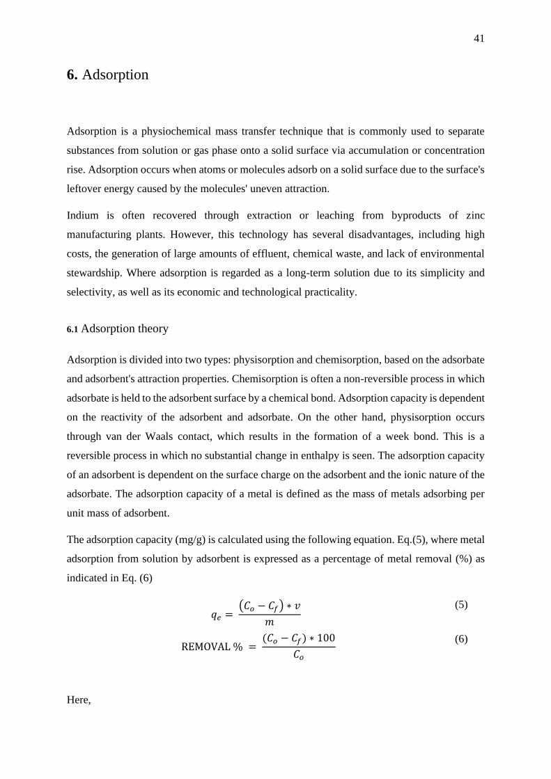
41
6. Adsorption
Adsorption is a physiochemical mass transfer technique that is commonly used to separate
substances from solution or gas phase onto a solid surface via accumulation or concentration
rise. Adsorption occurs when atoms or molecules adsorb on a solid surface due to the surface's
leftover energy caused by the molecules' uneven attraction.
Indium is often recovered through extraction or leaching from byproducts of zinc
manufacturing plants. However, this technology has several disadvantages, including high
costs, the generation of large amounts of effluent, chemical waste, and lack of environmental
stewardship. Where adsorption is regarded as a long-term solution due to its simplicity and
selectivity, as well as its economic and technological practicality.
6.1 Adsorption theory
Adsorption is divided into two types: physisorption and chemisorption, based on the adsorbate
and adsorbent's attraction properties. Chemisorption is often a non-reversible process in which
adsorbate is held to the adsorbent surface by a chemical bond. Adsorption capacity is dependent
on the reactivity of the adsorbent and adsorbate. On the other hand, physisorption occurs
through van der Waals contact, which results in the formation of a week bond. This is a
reversible process in which no substantial change in enthalpy is seen. The adsorption capacity
of an adsorbent is dependent on the surface charge on the adsorbent and the ionic nature of the
adsorbate. The adsorption capacity of a metal is defined as the mass of metals adsorbing per
unit mass of adsorbent.
The adsorption capacity (mg/g) is calculated using the following equation. Eq.(5), where metal
adsorption from solution by adsorbent is expressed as a percentage of metal removal (%) as
indicated in Eq. (6)
𝑞𝑒 = (𝐶𝑜 − 𝐶𝑓) ∗ 𝑣
𝑚
(5)
REMOVAL % = (𝐶𝑜 − 𝐶𝑓) ∗ 100
𝐶𝑜
(6)
Here,
42
q denotes the adsorption capacity in mg/g.
𝐶𝑜 denotes initial concentration in mg/L
𝐶𝑒 denotes equilibrium concentration in mg/L
v represents solution volume in mL
m denotes adsorbent mass in mg
6.2 Adsorption Isotherm
Adsorption isotherms are effective tools for analyzing the adsorption properties of various
adsorptive materials. Adsorption is a process that is often used to remove or recover valuable
materials from solution and continues until an equilibrium condition is reached. The
equilibrium state of adsorption is defined as the amount of adsorbate removed or recovered
from solution by per unit mass of adsorbent. Equation (5) mathematically describes the
equilibrium state that is used to determine the adsorbent capacity of various adsorbent materials
and able to reveal the equilibrium state of the adsorption process. There are many well-
established models that have been developed by various scientists throughout time to explain
the adsorption behavior of adsorbent. Giles et al. suggested four fundamental isotherm models
depending on the shape of the curve: the C isotherm, the L isotherm, the H isotherm, and the S
isotherm.(Giles, Smith and Huitson, 1974) Additionally, several concave isotherm models have
been developed since a single equation is incapable of adequately explain all mechanisms.
Langmuir, Freundlich, Redlich-Peterson, Sips, and Brunauer-Emmett-Teller (BET) are the
most often used isotherm models, with an extended version developed for multicomponent
systems using the Langmuir equation.
6.2.1 Basic isotherm category
This section will explain the four fundamental kinds of adsorption isotherms as shown in Figure
19. In isotherm plotting, the adsorbent capacity is shown on the Y axis and the equilibrium
concentration is plotted on the x axis.
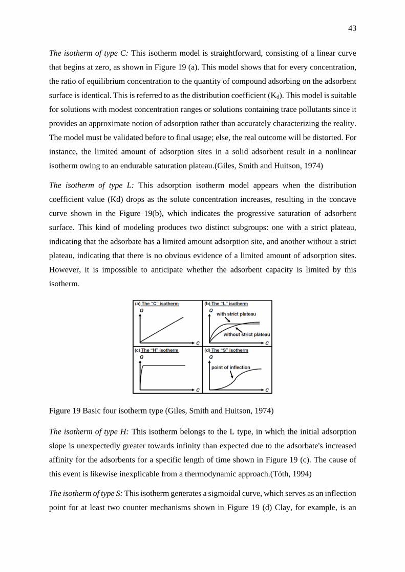
43
The isotherm of type C: This isotherm model is straightforward, consisting of a linear curve
that begins at zero, as shown in Figure 19 (a). This model shows that for every concentration,
the ratio of equilibrium concentration to the quantity of compound adsorbing on the adsorbent
surface is identical. This is referred to as the distribution coefficient (Kd). This model is suitable
for solutions with modest concentration ranges or solutions containing trace pollutants since it
provides an approximate notion of adsorption rather than accurately characterizing the reality.
The model must be validated before to final usage; else, the real outcome will be distorted. For
instance, the limited amount of adsorption sites in a solid adsorbent result in a nonlinear
isotherm owing to an endurable saturation plateau.(Giles, Smith and Huitson, 1974)
The isotherm of type L: This adsorption isotherm model appears when the distribution
coefficient value (Kd) drops as the solute concentration increases, resulting in the concave
curve shown in the Figure 19(b), which indicates the progressive saturation of adsorbent
surface. This kind of modeling produces two distinct subgroups: one with a strict plateau,
indicating that the adsorbate has a limited amount adsorption site, and another without a strict
plateau, indicating that there is no obvious evidence of a limited amount of adsorption sites.
However, it is impossible to anticipate whether the adsorbent capacity is limited by this
isotherm.
Figure 19 Basic four isotherm type (Giles, Smith and Huitson, 1974)
The isotherm of type H: This isotherm belongs to the L type, in which the initial adsorption
slope is unexpectedly greater towards infinity than expected due to the adsorbate's increased
affinity for the adsorbents for a specific length of time shown in Figure 19 (c). The cause of
this event is likewise inexplicable from a thermodynamic approach.(Tóth, 1994)
The isotherm of type S: This isotherm generates a sigmoidal curve, which serves as an inflection
point for at least two counter mechanisms shown in Figure 19 (d) Clay, for example, is an
44
adsorbent medium, and an adsorbent compound is a combination of nonpolar and other organic
compounds, but nonpolar organic compounds having a lower affinity for the clay and adsorbing
slowly. Other organic compounds, on the other hand, readily adsorb by the clay once non-polar
organic molecules have been absorbed.(Soheila Karimi-Lotfabad, Michael A. Pickard and
Murray R. Gray*, 1996) This is known as cooperative adsorption,(Hinz, 2001) and it occurs
often in surfactant adsorption.(Smith and Galan, 2002) Due to remnants of metal ligand
complex, the presence of metal species in the solution produces this kind of isotherm. During
this kind of adsorption, the metal-ligand adsorbs first, followed by the remainder of the
complex.(Bolt and van Olphen, 1985)
6.2.2 Langmuir isotherm
The Langmuir isotherm is a well-known model for explaining the equilibrium system of
adsorbate and adsorbent when the adsorption process is restricted to one component system.
Langmuir developed this adsorption model in 1918 to describe the behaviors of chemisorption
processes in which chemical bonds are generated to carry out the adsorption process,
particularly ionic bonds. To understand the concept, suppose that the solid has a finite
adsorption capacity qm, that all adsorbent sites are similar, that each adsorbent site can store a
single adsorbate, and that each adsorbent site retains energy to maintain adsorbate amount
independently. According to the assumption, the adsorption process proceeds as follows.
(Langmuir, 2002)
Free adsorbent site + adsorbate compound → complex formation on adsorbent surface
According to this assumption, fractional surface coverage is exactly proportional to the rate of
desorption, and in the equilibrium state the adsorption and desorption are equal shown in Eq.(7)
.
𝑘𝑎𝐶𝑒(1 − 𝜃) = 𝑘𝑑𝜃 (7)
Where ka stands for the adsorption rate constant, kd for the desorption rate constant, and Ce
(mg/L) for the equilibrium concentration.
The following equation represents more formal form of Langmuir equation (8):
𝜃 = 𝑞
𝑞𝑚=
𝐾𝐿𝐶𝑒
(1 + 𝐾𝐿𝐶𝑒)
(8)
45
Where,
𝐾𝐿 = 𝑘𝑎
𝑘𝑑
(9)
The adsorbent capacity is denoted by q, while the quantity of adsorbate held on the adsorbent
surface in a single monolayer is denoted by qm (mg/g) (alternatively called maximum
adsorption capacity).
In general, the Langmuir isotherm model assumes that each adsorbate chemical occupies its
own adsorbent site and that there is no interaction between two neighboring compounds on a
homogenous surface. The following are the nonlinear Eq.(10)(11) and linear equations for the
Langmuir isotherm model:
𝑞𝑒 =𝑞𝑚𝐾𝐿𝐶𝑒
(1 + 𝐾𝐿𝐶𝑒) (non − linear form)
(10)
1
𝑞𝑒=
1
𝐾𝐿𝑞𝑚𝐶𝑒+
1
𝑞𝑚 (Linear form)
(11)
Where, 𝑞𝑒 (mg/g) is the concentration of adsorbate in the surface of adsorbent in the
equilibrium state and KL (L/mg) denotes the Langmuir constant.(Liu et al., 2019)
Another significant factor in the Langmuir isotherm is the factor of separation or equilibrium
parameter, which is denoted by RL and can be expressed as
𝑅𝐿 = 1
1 + 𝐾𝐿𝐶𝑜
(12)
Where Co signifies the initial concentration of the solution, and the RL value is used to assess
the Langmuir model's fit for the adsorption process. RL value more than one indicates an
unfavorable process, whereas a value greater than zero or less than one indicates a favorable
process, and RL value of zero indicates an irreversible process (Wang, Wang and Ma, 2010).
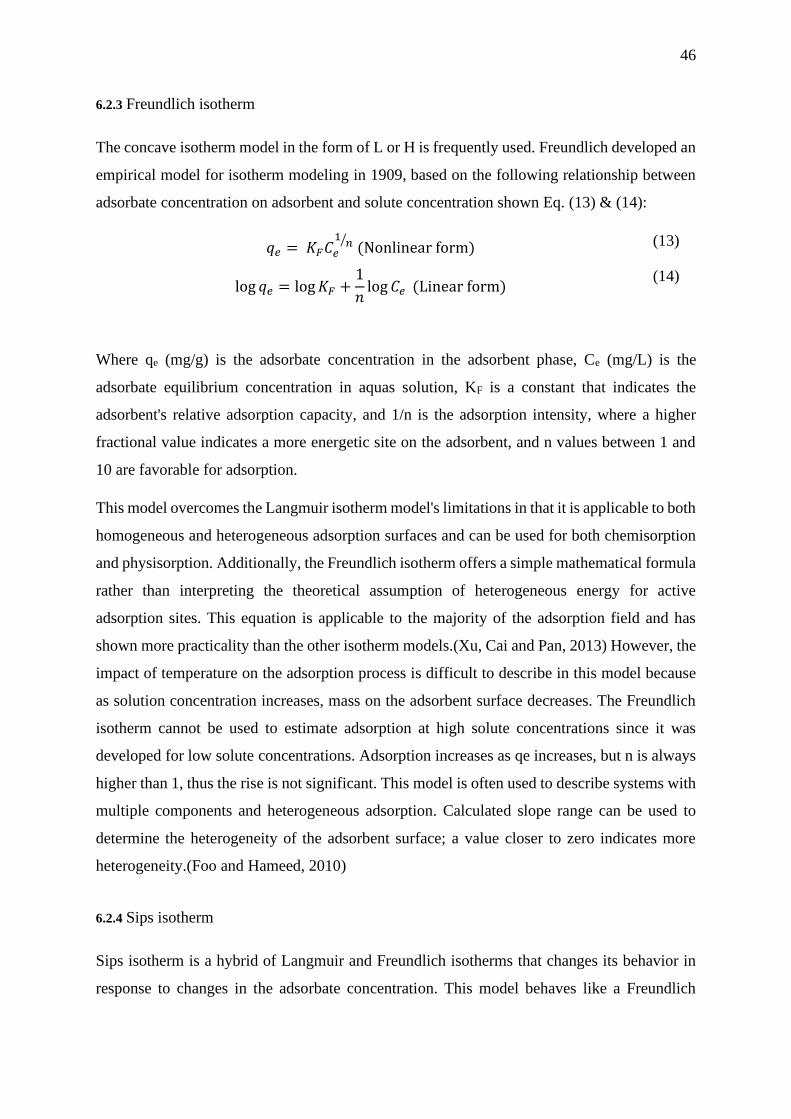
46
6.2.3 Freundlich isotherm
The concave isotherm model in the form of L or H is frequently used. Freundlich developed an
empirical model for isotherm modeling in 1909, based on the following relationship between
adsorbate concentration on adsorbent and solute concentration shown Eq. (13) & (14):
𝑞𝑒 = 𝐾𝐹𝐶𝑒
1𝑛⁄
(Nonlinear form) (13)
log 𝑞𝑒 = log 𝐾𝐹 +1
𝑛log 𝐶𝑒 (Linear form)
(14)
Where qe (mg/g) is the adsorbate concentration in the adsorbent phase, Ce (mg/L) is the
adsorbate equilibrium concentration in aquas solution, KF is a constant that indicates the
adsorbent's relative adsorption capacity, and 1/n is the adsorption intensity, where a higher
fractional value indicates a more energetic site on the adsorbent, and n values between 1 and
10 are favorable for adsorption.
This model overcomes the Langmuir isotherm model's limitations in that it is applicable to both
homogeneous and heterogeneous adsorption surfaces and can be used for both chemisorption
and physisorption. Additionally, the Freundlich isotherm offers a simple mathematical formula
rather than interpreting the theoretical assumption of heterogeneous energy for active
adsorption sites. This equation is applicable to the majority of the adsorption field and has
shown more practicality than the other isotherm models.(Xu, Cai and Pan, 2013) However, the
impact of temperature on the adsorption process is difficult to describe in this model because
as solution concentration increases, mass on the adsorbent surface decreases. The Freundlich
isotherm cannot be used to estimate adsorption at high solute concentrations since it was
developed for low solute concentrations. Adsorption increases as qe increases, but n is always
higher than 1, thus the rise is not significant. This model is often used to describe systems with
multiple components and heterogeneous adsorption. Calculated slope range can be used to
determine the heterogeneity of the adsorbent surface; a value closer to zero indicates more
heterogeneity.(Foo and Hameed, 2010)
6.2.4 Sips isotherm
Sips isotherm is a hybrid of Langmuir and Freundlich isotherms that changes its behavior in
response to changes in the adsorbate concentration. This model behaves like a Freundlich
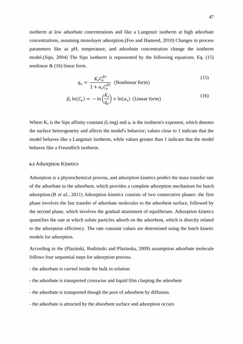
47
isotherm at low adsorbate concentrations and like a Langmuir isotherm at high adsorbate
concentrations, assuming monolayer adsorption.(Foo and Hameed, 2010) Changes in process
parameters like as pH, temperature, and adsorbate concentration change the isotherm
model.(Sips, 2004) The Sips isotherm is represented by the following equations. Eq. (15)
nonlinear & (16) linear form.
𝑞𝑒 = 𝐾𝑠𝐶𝑒
𝛽𝑠
1 + 𝑎𝑠𝐶𝑒𝛽𝑠
(Nonlinear form) (15)
𝛽𝑠 ln(𝐶𝑒) = − ln (𝐾𝑠
𝑞𝑒) + ln(𝑎𝑠) (Linear form)
(16)
Where Ks is the Sips affinity constant (L/mg) and as is the isotherm's exponent, which denotes
the surface heterogeneity and affects the model's behavior; values close to 1 indicate that the
model behaves like a Langmuir isotherm, while values greater than 1 indicate that the model
behaves like a Freundlich isotherm.
6.3 Adsorption Kinetics
Adsorption is a physiochemical process, and adsorption kinetics predict the mass transfer rate
of the adsorbate to the adsorbent, which provides a complete adsorption mechanism for batch
adsorption.(B et al., 2011) Adsorption kinetics consists of two consecutive phases: the first
phase involves the fast transfer of adsorbate molecules to the adsorbent surface, followed by
the second phase, which involves the gradual attainment of equilibrium. Adsorption kinetics
quantifies the rate at which solute particles adsorb on the adsorbent, which is directly related
to the adsorption efficiency. The rate constant values are determined using the batch kinetic
models for adsorption.
According to the (Plazinski, Rudzinski and Plazinska, 2009) assumption adsorbate molecule
follows four sequential steps for adsorption process.
- the adsorbate is carried inside the bulk in solution
- the adsorbate is transported crosswise and liquid film clasping the adsorbent
- the adsorbate is transported though the pore of adsorbent by diffusion.
- the adsorbate is attracted by the absorbent surface and adsorption occurs
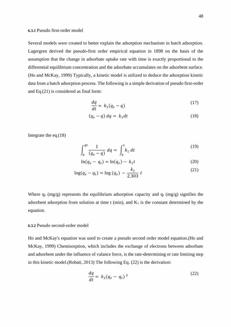
48
6.3.1 Pseudo first-order model
Several models were created to better explain the adsorption mechanism in batch adsorption.
Lagergren derived the pseudo-first order empirical equation in 1898 on the basis of the
assumption that the change in adsorbate uptake rate with time is exactly proportional to the
differential equilibrium concentration and the adsorbate accumulates on the adsorbent surface.
(Ho and McKay, 1999) Typically, a kinetic model is utilized to deduce the adsorption kinetic
data from a batch adsorption process. The following is a simple derivation of pseudo first-order
and Eq.(21) is considered as final form:
𝑑𝑞
𝑑𝑡= 𝑘1(𝑞𝑒 − 𝑞)
(17)
(𝑞𝑒 − 𝑞) 𝑑𝑞 = 𝑘1𝑑𝑡 (18)
Integrate the eq.(18)
∫1
(𝑞𝑒 − 𝑞)
𝑞𝑡
0
𝑑𝑞 = ∫ 𝑘1 𝑑𝑡𝑡
0
(19)
ln(𝑞𝑒 − 𝑞𝑡) = ln(𝑞𝑒) − 𝑘1𝑡 (20)
log(𝑞𝑒 − 𝑞𝑡) = log (𝑞𝑒) − 𝑘1
2.303 𝑡
(21)
Where qe (mg/g) represents the equilibrium adsorption capacity and qt (mg/g) signifies the
adsorbent adsorption from solution at time t (min), and K1 is the constant determined by the
equation.
6.3.2 Pseudo second-order model
Ho and McKay's equation was used to create a pseudo second order model equation.(Ho and
McKay, 1999) Chemisorption, which includes the exchange of electrons between adsorbate
and adsorbent under the influence of valance force, is the rate-determining or rate limiting step
in this kinetic model.(Robati, 2013) The following Eq. (22) is the derivation:
𝑑𝑞
𝑑𝑡= 𝑘2(𝑞𝑒 − 𝑞𝑡) 2
(22)
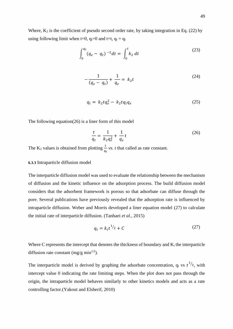
49
Where, K2 is the coefficient of pseudo second order rate, by taking integration in Eq. (22) by
using following limit when t=0, qt=0 and t=t, qt = qt
∫ (𝑞𝑒 − 𝑞𝑡) −2𝑑𝑡 = ∫ 𝑘2 𝑑𝑡𝑡
0
𝑞𝑡
0
(23)
−1
(𝑞𝑒 − 𝑞𝑡)+
1
𝑞𝑒 = 𝑘2𝑡
(24)
𝑞𝑡 = 𝑘2𝑡𝑞𝑒2 − 𝑘2𝑡𝑞𝑡𝑞𝑒 (25)
The following equation(26) is a liner form of this model
𝑡
𝑞𝑡=
1
𝑘2𝑞𝑒2
+ 1
𝑞𝑒𝑡
(26)
The K2 values is obtained from plotting 𝑡
𝑞𝑡 vs. t that called as rate constant.
6.3.3 Intraparticle diffusion model
The interparticle diffusion model was used to evaluate the relationship between the mechanism
of diffusion and the kinetic influence on the adsorption process. The build diffusion model
considers that the adsorbent framework is porous so that adsorbate can diffuse through the
pore. Several publications have previously revealed that the adsorption rate is influenced by
intraparticle diffusion. Weber and Morris developed a liner equation model (27) to calculate
the initial rate of interparticle diffusion. (Tanhaei et al., 2015)
𝑞𝑡 = 𝑘𝑖𝑡1
2⁄ + 𝐶
(27)
Where C represents the intercept that denotes the thickness of boundary and Ki the interparticle
diffusion rate constant (mg/g min1/2).
The interparticle model is derived by graphing the adsorbate concentration, qt vs 𝑡1
2⁄ , with
intercept value 0 indicating the rate limiting steps. When the plot does not pass through the
origin, the intraparticle model behaves similarly to other kinetics models and acts as a rate
controlling factor.(Yakout and Elsherif, 2010)
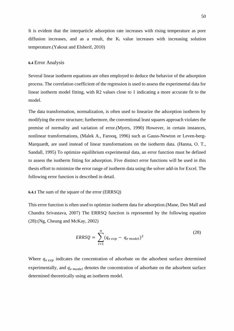
50
It is evident that the interparticle adsorption rate increases with rising temperature as pore
diffusion increases, and as a result, the Ki value increases with increasing solution
temperature.(Yakout and Elsherif, 2010)
6.4 Error Analysis
Several linear isotherm equations are often employed to deduce the behavior of the adsorption
process. The correlation coefficient of the regression is used to assess the experimental data for
linear isotherm model fitting, with R2 values close to 1 indicating a more accurate fit to the
model.
The data transformation, normalization, is often used to linearize the adsorption isotherm by
modifying the error structure; furthermore, the conventional least squares approach violates the
premise of normality and variation of error.(Myers, 1990) However, in certain instances,
nonlinear transformations, (Malek A., Farooq, 1996) such as Gauss-Newton or Leven-berg-
Marquardt, are used instead of linear transformations on the isotherm data. (Hanna, O. T.,
Sandall, 1995) To optimize equilibrium experimental data, an error function must be defined
to assess the isotherm fitting for adsorption. Five distinct error functions will be used in this
thesis effort to minimize the error range of isotherm data using the solver add-in for Excel. The
following error function is described in detail.
6.4.1 The sum of the square of the error (ERRSQ)
This error function is often used to optimize isotherm data for adsorption.(Mane, Deo Mall and
Chandra Srivastava, 2007) The ERRSQ function is represented by the following equation
(28):(Ng, Cheung and McKay, 2002)
𝐸𝑅𝑅𝑆𝑄 = ∑(𝑞𝑒 𝑒𝑥𝑝 − 𝑞𝑒 𝑚𝑜𝑑𝑒𝑙)2
𝑛
𝑖=1
(28)
Where 𝑞𝑒 𝑒𝑥𝑝 indicates the concentration of adsorbate on the adsorbent surface determined
experimentally, and 𝑞𝑒 𝑚𝑜𝑑𝑒𝑙 denotes the concentration of adsorbate on the adsorbent surface
determined theoretically using an isotherm model.
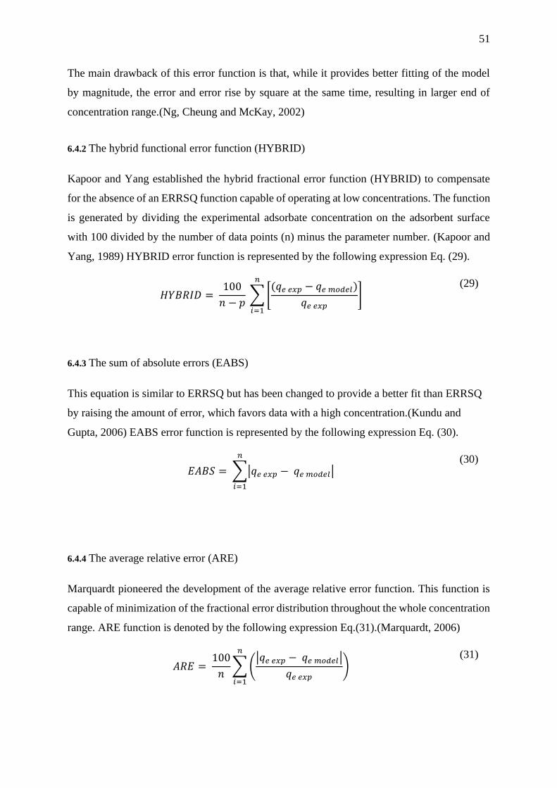
51
The main drawback of this error function is that, while it provides better fitting of the model
by magnitude, the error and error rise by square at the same time, resulting in larger end of
concentration range.(Ng, Cheung and McKay, 2002)
6.4.2 The hybrid functional error function (HYBRID)
Kapoor and Yang established the hybrid fractional error function (HYBRID) to compensate
for the absence of an ERRSQ function capable of operating at low concentrations. The function
is generated by dividing the experimental adsorbate concentration on the adsorbent surface
with 100 divided by the number of data points (n) minus the parameter number. (Kapoor and
Yang, 1989) HYBRID error function is represented by the following expression Eq. (29).
𝐻𝑌𝐵𝑅𝐼𝐷 = 100
𝑛 − 𝑝 ∑ [
(𝑞𝑒 𝑒𝑥𝑝 − 𝑞𝑒 𝑚𝑜𝑑𝑒𝑙)
𝑞𝑒 𝑒𝑥𝑝]
𝑛
𝑖=1
(29)
6.4.3 The sum of absolute errors (EABS)
This equation is similar to ERRSQ but has been changed to provide a better fit than ERRSQ
by raising the amount of error, which favors data with a high concentration.(Kundu and
Gupta, 2006) EABS error function is represented by the following expression Eq. (30).
𝐸𝐴𝐵𝑆 = ∑|𝑞𝑒 𝑒𝑥𝑝 − 𝑞𝑒 𝑚𝑜𝑑𝑒𝑙|
𝑛
𝑖=1
(30)
6.4.4 The average relative error (ARE)
Marquardt pioneered the development of the average relative error function. This function is
capable of minimization of the fractional error distribution throughout the whole concentration
range. ARE function is denoted by the following expression Eq.(31).(Marquardt, 2006)
𝐴𝑅𝐸 = 100
𝑛∑ (
|𝑞𝑒 𝑒𝑥𝑝 − 𝑞𝑒 𝑚𝑜𝑑𝑒𝑙|
𝑞𝑒 𝑒𝑥𝑝)
𝑛
𝑖=1
(31)
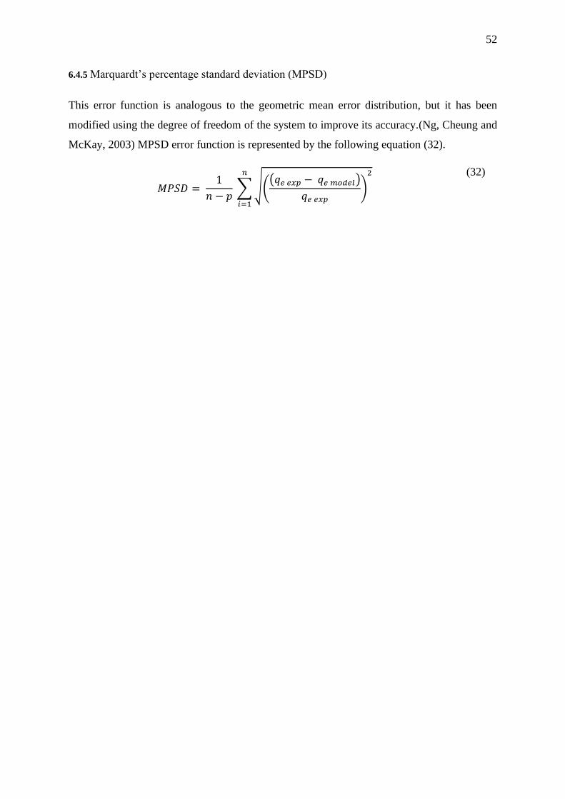
52
6.4.5 Marquardt’s percentage standard deviation (MPSD)
This error function is analogous to the geometric mean error distribution, but it has been
modified using the degree of freedom of the system to improve its accuracy.(Ng, Cheung and
McKay, 2003) MPSD error function is represented by the following equation (32).
𝑀𝑃𝑆𝐷 = 1
𝑛 − 𝑝 ∑ √(
(𝑞𝑒 𝑒𝑥𝑝 − 𝑞𝑒 𝑚𝑜𝑑𝑒𝑙)
𝑞𝑒 𝑒𝑥𝑝)
2𝑛
𝑖=1
(32)
53
7. Experimental Procedure
The adsorption experiments for Indium were done in batch mode. To begin, batch
experiments were done utilizing granular ion exchange resin to evaluate the materials' Indium
adsorption behavior. The following parameters are investigated to better understand the
adsorbent's adoption mechanism: effect of pH, the influence of contact time, the effect of
starting concentration, and the equilibrium isotherm (Sekhararaoogulipalli, Prasad and
Wasewar, 2011). The entire method (shown in Figure 22) was followed in this thesis for
adsorbent materials (Lewatit TP-207, Lewatit TP-260, and Amberlite IRA 742) in order to
evaluate the functionality of Indium adsorption and the optimal adsorption parameters. Later
on, the Indium adsorption functional materials were selected by a batch adsorption procedure,
and the materials were used to fabricate a 3D printed adsorbent module for use in the study.
The batch adsorption and recovery method for Indium was carried out, as well regeneration
study of a 3D printed adsorbent module.
The weight of all solid materials used in dosing was determined using a standard scale
(METTLER AE240), whereas liquid samples and reagents were determined using an electronic
pipette (Sartorius). The pH of the adsorbate-containing solution was adjusted, and the solution
temperature was measured using a Metrohm 744 pH meter. All adsorption experiments were
conducted in batch mode at room temperature. The solution was mixed with a constant rotation
speed using an EDMUND BULER KS10 shaker (300 rpm).
Following each batch adsorption of granular ion exchange resin, the adsorbent was removed
from the solution using a syringe filter with a pore size of 0.20𝜇m and a diameter of 26mm.
The filtrated samples were promptly refrigerated until ICP measurement. The metal ion
concentration in solution was determined by ICP analysis with an AGILENT
TECHNOLOGIES 7900. This thesis work investigated the adsorbent's selectivity for the
Indium ion. All experiments and analyses were conducted at the chemical laboratory at LUT.
7.1 Materials and Methods
This chapter will describe the materials used in the whole thesis work and methods used for
carrying out the research work.
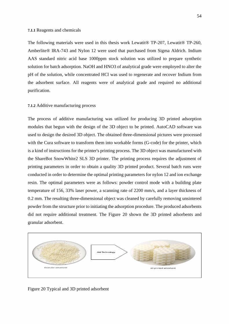
54
7.1.1 Reagents and chemicals
The following materials were used in this thesis work Lewatit® TP-207, Lewatit® TP-260,
Amberlite® IRA-743 and Nylon 12 were used that purchased from Sigma Aldrich. Indium
AAS standard nitric acid base 1000ppm stock solution was utilized to prepare synthetic
solution for batch adsorption. NaOH and HNO3 of analytical grade were employed to alter the
pH of the solution, while concentrated HCl was used to regenerate and recover Indium from
the adsorbent surface. All reagents were of analytical grade and required no additional
purification.
7.1.2 Additive manufacturing process
The process of additive manufacturing was utilized for producing 3D printed adsorption
modules that begun with the design of the 3D object to be printed. AutoCAD software was
used to design the desired 3D object. The obtained three-dimensional pictures were processed
with the Cura software to transform them into workable forms (G-code) for the printer, which
is a kind of instructions for the printer's printing process. The 3D object was manufactured with
the ShareBot SnowWhite2 SLS 3D printer. The printing process requires the adjustment of
printing parameters in order to obtain a quality 3D printed product. Several batch runs were
conducted in order to determine the optimal printing parameters for nylon 12 and ion exchange
resin. The optimal parameters were as follows: powder control mode with a building plate
temperature of 156, 33% laser power, a scanning rate of 2200 mm/s, and a layer thickness of
0.2 mm. The resulting three-dimensional object was cleaned by carefully removing unsintered
powder from the structure prior to initiating the adsorption procedure. The produced adsorbents
did not require additional treatment. The Figure 20 shown the 3D printed adsorbents and
granular adsorbent.
Figure 20 Typical and 3D printed adsorbent
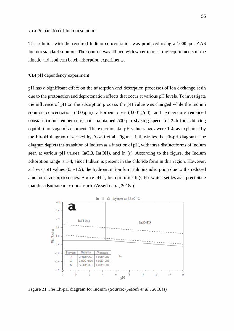
55
7.1.3 Preparation of Indium solution
The solution with the required Indium concentration was produced using a 1000ppm AAS
Indium standard solution. The solution was diluted with water to meet the requirements of the
kinetic and isotherm batch adsorption experiments.
7.1.4 pH dependency experiment
pH has a significant effect on the adsorption and desorption processes of ion exchange resin
due to the protonation and deprotonation effects that occur at various pH levels. To investigate
the influence of pH on the adsorption process, the pH value was changed while the Indium
solution concentration (100ppm), adsorbent dose (0.001g/ml), and temperature remained
constant (room temperature) and maintained 500rpm shaking speed for 24h for achieving
equilibrium stage of adsorbent. The experimental pH value ranges were 1-4, as explained by
the Eh-pH diagram described by Assefi et al. Figure 21 illustrates the Eh-pH diagram. The
diagram depicts the transition of Indium as a function of pH, with three distinct forms of Indium
seen at various pH values: InCl3, In(OH), and In (s). According to the figure, the Indium
adsorption range is 1-4, since Indium is present in the chloride form in this region. However,
at lower pH values (0.5-1.5), the hydronium ion form inhibits adsorption due to the reduced
amount of adsorption sites. Above pH 4, Indium forms In(OH), which settles as a precipitate
that the adsorbate may not absorb. (Assefi et al., 2018a)
Figure 21 The Eh-pH diagram for Indium (Source: (Assefi et al., 2018a))
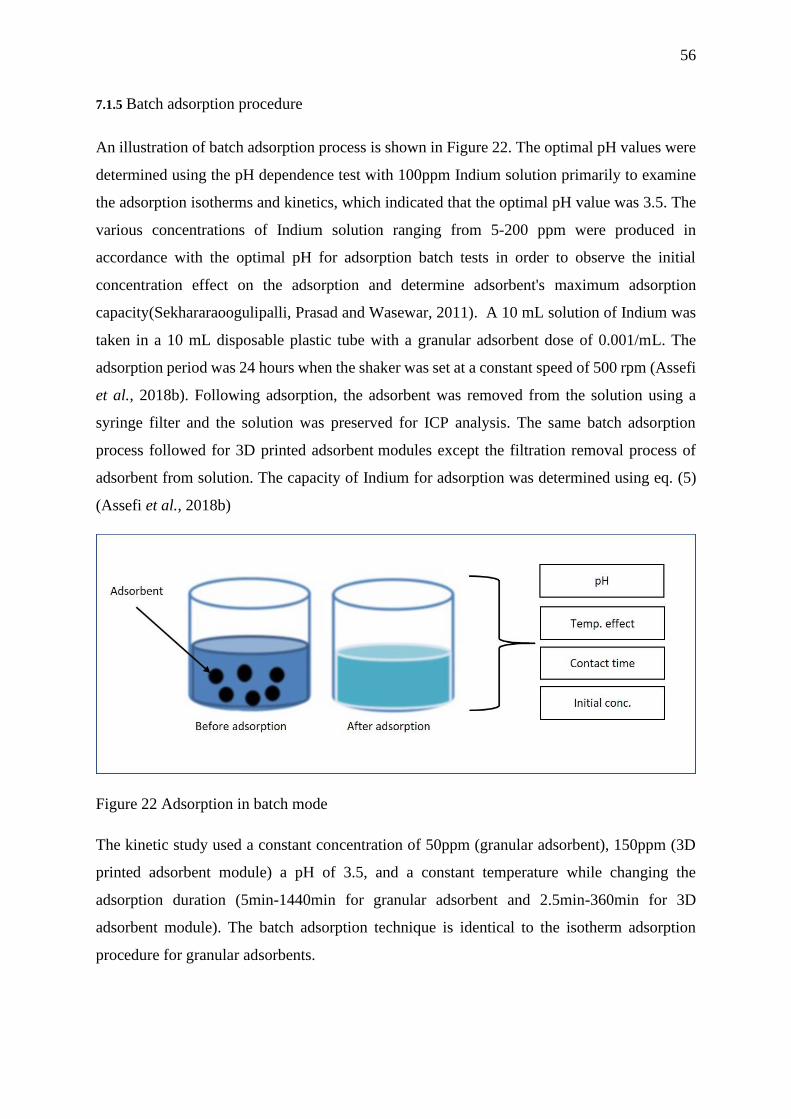
56
7.1.5 Batch adsorption procedure
An illustration of batch adsorption process is shown in Figure 22. The optimal pH values were
determined using the pH dependence test with 100ppm Indium solution primarily to examine
the adsorption isotherms and kinetics, which indicated that the optimal pH value was 3.5. The
various concentrations of Indium solution ranging from 5-200 ppm were produced in
accordance with the optimal pH for adsorption batch tests in order to observe the initial
concentration effect on the adsorption and determine adsorbent's maximum adsorption
capacity(Sekhararaoogulipalli, Prasad and Wasewar, 2011). A 10 mL solution of Indium was
taken in a 10 mL disposable plastic tube with a granular adsorbent dose of 0.001/mL. The
adsorption period was 24 hours when the shaker was set at a constant speed of 500 rpm (Assefi
et al., 2018b). Following adsorption, the adsorbent was removed from the solution using a
syringe filter and the solution was preserved for ICP analysis. The same batch adsorption
process followed for 3D printed adsorbent modules except the filtration removal process of
adsorbent from solution. The capacity of Indium for adsorption was determined using eq. (5)
(Assefi et al., 2018b)
Figure 22 Adsorption in batch mode
The kinetic study used a constant concentration of 50ppm (granular adsorbent), 150ppm (3D
printed adsorbent module) a pH of 3.5, and a constant temperature while changing the
adsorption duration (5min-1440min for granular adsorbent and 2.5min-360min for 3D
adsorbent module). The batch adsorption technique is identical to the isotherm adsorption
procedure for granular adsorbents.
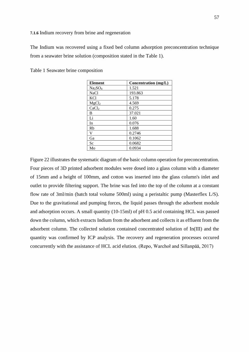
57
7.1.6 Indium recovery from brine and regeneration
The Indium was recovered using a fixed bed column adsorption preconcentration technique
from a seawater brine solution (composition stated in the Table 1).
Table 1 Seawater brine composition
Element Concentration (mg/L)
Na2SO4 1.521
NaCl 193.863
KCl 5.178
MgCl2 4.569
CaCl2 0.275
B 37.021
Li 1.60
In 0.076
Rb 1.688
V 0.2746
Ga 0.1062
Sc 0.0682
Mo 0.0934
Figure 22 illustrates the systematic diagram of the basic column operation for preconcentration.
Four pieces of 3D printed adsorbent modules were dosed into a glass column with a diameter
of 15mm and a height of 100mm, and cotton was inserted into the glass column's inlet and
outlet to provide filtering support. The brine was fed into the top of the column at a constant
flow rate of 3ml/min (batch total volume 500ml) using a peristaltic pump (Masterflex L/S).
Due to the gravitational and pumping forces, the liquid passes through the adsorbent module
and adsorption occurs. A small quantity (10-15ml) of pH 0.5 acid containing HCL was passed
down the column, which extracts Indium from the adsorbent and collects it as effluent from the
adsorbent column. The collected solution contained concentrated solution of In(III) and the
quantity was confirmed by ICP analysis. The recovery and regeneration processes occured
concurrently with the assistance of HCL acid elution. (Repo, Warchoł and Sillanpää, 2017)
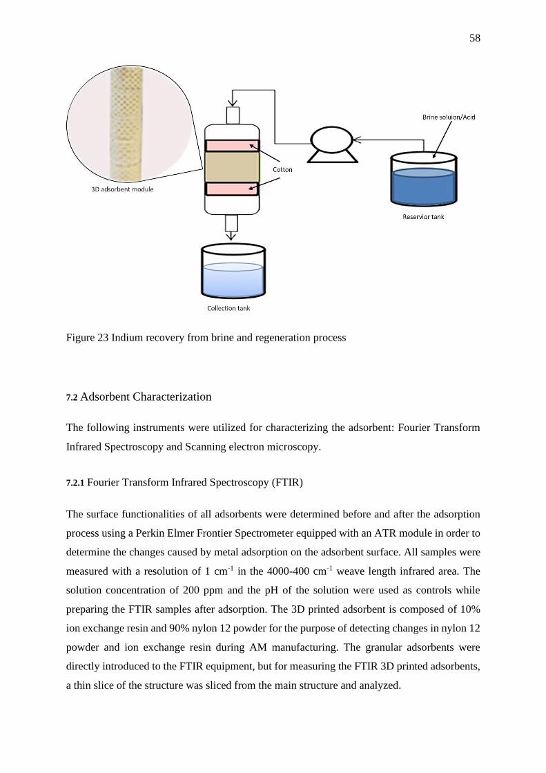
58
Figure 23 Indium recovery from brine and regeneration process
7.2 Adsorbent Characterization
The following instruments were utilized for characterizing the adsorbent: Fourier Transform
Infrared Spectroscopy and Scanning electron microscopy.
7.2.1 Fourier Transform Infrared Spectroscopy (FTIR)
The surface functionalities of all adsorbents were determined before and after the adsorption
process using a Perkin Elmer Frontier Spectrometer equipped with an ATR module in order to
determine the changes caused by metal adsorption on the adsorbent surface. All samples were
measured with a resolution of 1 cm-1 in the 4000-400 cm-1 weave length infrared area. The
solution concentration of 200 ppm and the pH of the solution were used as controls while
preparing the FTIR samples after adsorption. The 3D printed adsorbent is composed of 10%
ion exchange resin and 90% nylon 12 powder for the purpose of detecting changes in nylon 12
powder and ion exchange resin during AM manufacturing. The granular adsorbents were
directly introduced to the FTIR equipment, but for measuring the FTIR 3D printed adsorbents,
a thin slice of the structure was sliced from the main structure and analyzed.

59
7.2.2 Scanning Electron Microscopy
The adsorbent's morphology was studied using the available SEM instrument at LUT
University, model Hitachi SU 3500, which combines with EDS analysis. Adsorbent samples
were prepared prior to and after adsorption in accordance with SEM's standard operating
procedures for morphology and elemental analysis. The high vacuum condition was employed
for the SEM analysis, and the acceleration voltage was 15KV.
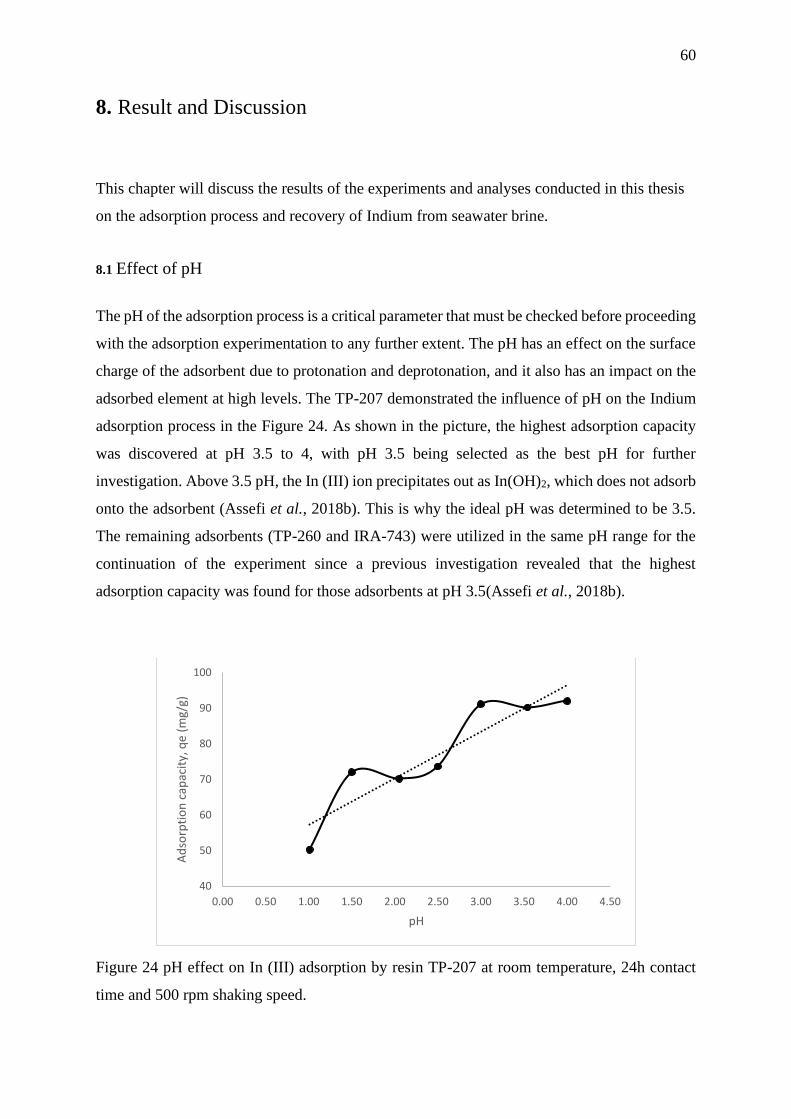
60
8. Result and Discussion
This chapter will discuss the results of the experiments and analyses conducted in this thesis
on the adsorption process and recovery of Indium from seawater brine.
8.1 Effect of pH
The pH of the adsorption process is a critical parameter that must be checked before proceeding
with the adsorption experimentation to any further extent. The pH has an effect on the surface
charge of the adsorbent due to protonation and deprotonation, and it also has an impact on the
adsorbed element at high levels. The TP-207 demonstrated the influence of pH on the Indium
adsorption process in the Figure 24. As shown in the picture, the highest adsorption capacity
was discovered at pH 3.5 to 4, with pH 3.5 being selected as the best pH for further
investigation. Above 3.5 pH, the In (III) ion precipitates out as In(OH)2, which does not adsorb
onto the adsorbent (Assefi et al., 2018b). This is why the ideal pH was determined to be 3.5.
The remaining adsorbents (TP-260 and IRA-743) were utilized in the same pH range for the
continuation of the experiment since a previous investigation revealed that the highest
adsorption capacity was found for those adsorbents at pH 3.5(Assefi et al., 2018b).
Figure 24 pH effect on In (III) adsorption by resin TP-207 at room temperature, 24h contact
time and 500 rpm shaking speed.
40
50
60
70
80
90
100
0.00 0.50 1.00 1.50 2.00 2.50 3.00 3.50 4.00 4.50
Ad
sorp
tio
n c
apac
ity,
qe
(mg/
g)
pH
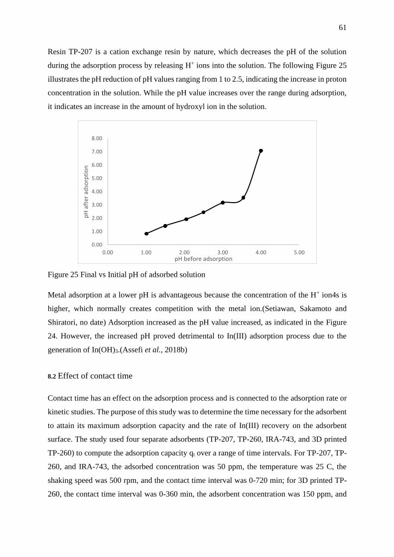
61
Resin TP-207 is a cation exchange resin by nature, which decreases the pH of the solution
during the adsorption process by releasing H+ ions into the solution. The following Figure 25
illustrates the pH reduction of pH values ranging from 1 to 2.5, indicating the increase in proton
concentration in the solution. While the pH value increases over the range during adsorption,
it indicates an increase in the amount of hydroxyl ion in the solution.
Figure 25 Final vs Initial pH of adsorbed solution
Metal adsorption at a lower pH is advantageous because the concentration of the H+ ion4s is
higher, which normally creates competition with the metal ion.(Setiawan, Sakamoto and
Shiratori, no date) Adsorption increased as the pH value increased, as indicated in the Figure
24. However, the increased pH proved detrimental to In(III) adsorption process due to the
generation of In(OH)3.(Assefi et al., 2018b)
8.2 Effect of contact time
Contact time has an effect on the adsorption process and is connected to the adsorption rate or
kinetic studies. The purpose of this study was to determine the time necessary for the adsorbent
to attain its maximum adsorption capacity and the rate of In(III) recovery on the adsorbent
surface. The study used four separate adsorbents (TP-207, TP-260, IRA-743, and 3D printed
TP-260) to compute the adsorption capacity qt over a range of time intervals. For TP-207, TP-
260, and IRA-743, the adsorbed concentration was 50 ppm, the temperature was 25 C, the
shaking speed was 500 rpm, and the contact time interval was 0-720 min; for 3D printed TP-
260, the contact time interval was 0-360 min, the adsorbent concentration was 150 ppm, and
0.00
1.00
2.00
3.00
4.00
5.00
6.00
7.00
8.00
0.00 1.00 2.00 3.00 4.00 5.00
pH
aft
er a
dso
rpti
on
pH before adsorption
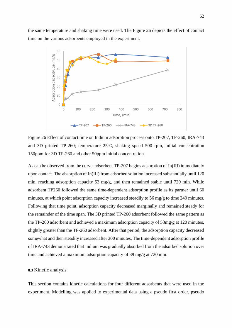
62
the same temperature and shaking time were used. The Figure 26 depicts the effect of contact
time on the various adsorbents employed in the experiment.
Figure 26 Effect of contact time on Indium adsorption process onto TP-207, TP-260, IRA-743
and 3D printed TP-260; temperature 25℃, shaking speed 500 rpm, initial concentration
150ppm for 3D TP-260 and other 50ppm initial concentration.
As can be observed from the curve, adsorbent TP-207 begins adsorption of In(III) immediately
upon contact. The absorption of In(III) from adsorbed solution increased substantially until 120
min, reaching adsorption capacity 53 mg/g, and then remained stable until 720 min. While
adsorbent TP260 followed the same time-dependent adsorption profile as its partner until 60
minutes, at which point adsorption capacity increased steadily to 56 mg/g to time 240 minutes.
Following that time point, adsorption capacity decreased marginally and remained steady for
the remainder of the time span. The 3D printed TP-260 adsorbent followed the same pattern as
the TP-260 adsorbent and achieved a maximum adsorption capacity of 53mg/g at 120 minutes,
slightly greater than the TP-260 adsorbent. After that period, the adsorption capacity decreased
somewhat and then steadily increased after 300 minutes. The time-dependent adsorption profile
of IRA-743 demonstrated that Indium was gradually absorbed from the adsorbed solution over
time and achieved a maximum adsorption capacity of 39 mg/g at 720 min.
8.3 Kinetic analysis
This section contains kinetic calculations for four different adsorbents that were used in the
experiment. Modelling was applied to experimental data using a pseudo first order, pseudo
0
10
20
30
40
50
60
0 100 200 300 400 500 600 700 800
Ad
sorp
tio
n c
apac
ity,
qe,
mg/
g
Time, (min)
TP-207 TP-260 IRA-743 3D TP-260
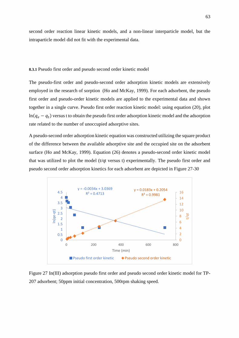
63
second order reaction linear kinetic models, and a non-linear interparticle model, but the
intraparticle model did not fit with the experimental data.
8.3.1 Pseudo first order and pseudo second order kinetic model
The pseudo-first order and pseudo-second order adsorption kinetic models are extensively
employed in the research of sorption (Ho and McKay, 1999). For each adsorbent, the pseudo
first order and pseudo-order kinetic models are applied to the experimental data and shown
together in a single curve. Pseudo first order reaction kinetic model: using equation (20), plot
ln(𝑞𝑒 − 𝑞𝑡) versus t to obtain the pseudo first order adsorption kinetic model and the adsorption
rate related to the number of unoccupied adsorptive sites.
A pseudo-second order adsorption kinetic equation was constructed utilizing the square product
of the difference between the available adsorptive site and the occupied site on the adsorbent
surface (Ho and McKay, 1999). Equation (26) denotes a pseudo-second order kinetic model
that was utilized to plot the model (t/qt versus t) experimentally. The pseudo first order and
pseudo second order adsorption kinetics for each adsorbent are depicted in Figure 27-30
Figure 27 In(III) adsorption pseudo first order and pseudo second order kinetic model for TP-
207 adsorbent; 50ppm initial concentration, 500rpm shaking speed.
y = -0.0034x + 3.0369R² = 0.4713
y = 0.0183x + 0.2054R² = 0.9981
0
2
4
6
8
10
12
14
16
0
0.5
1
1.5
2
2.5
3
3.5
4
4.5
0 200 400 600 800
t/q
t
ln(q
e-q
t)
Time (min)
Pseudo first order kinetic Pseudo second order kinetic
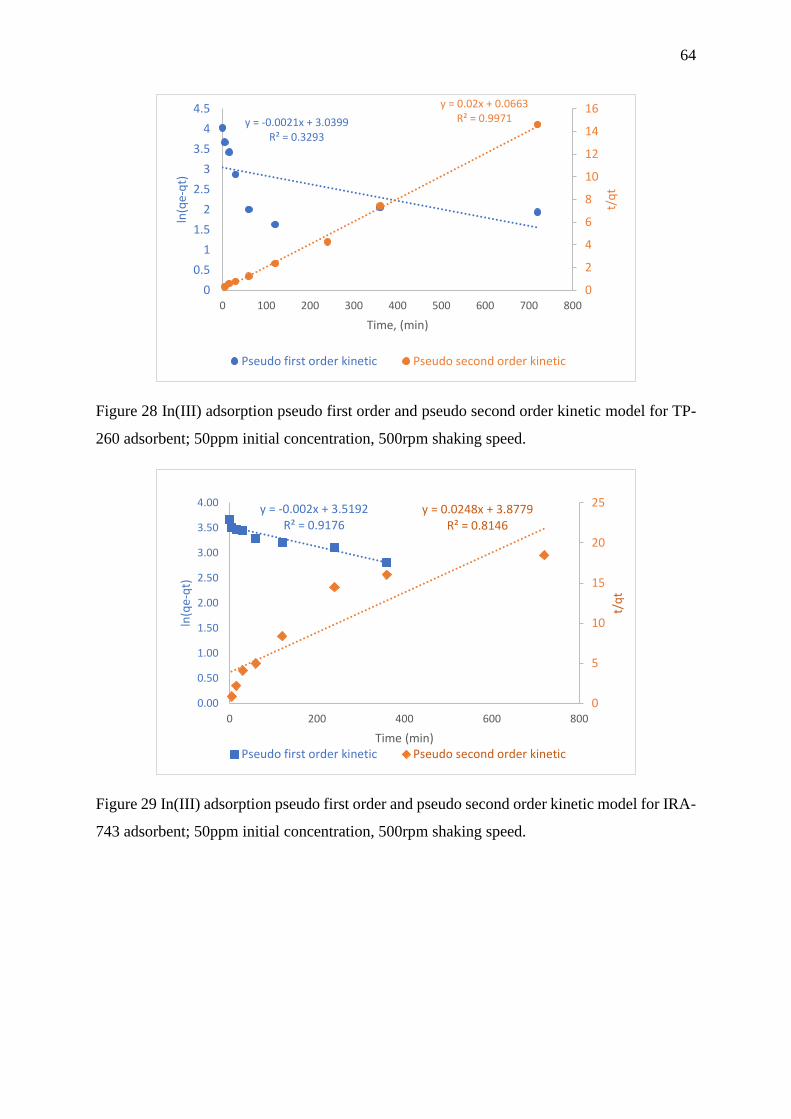
64
Figure 28 In(III) adsorption pseudo first order and pseudo second order kinetic model for TP-
260 adsorbent; 50ppm initial concentration, 500rpm shaking speed.
Figure 29 In(III) adsorption pseudo first order and pseudo second order kinetic model for IRA-
743 adsorbent; 50ppm initial concentration, 500rpm shaking speed.
y = -0.0021x + 3.0399R² = 0.3293
y = 0.02x + 0.0663R² = 0.9971
0
2
4
6
8
10
12
14
16
0
0.5
1
1.5
2
2.5
3
3.5
4
4.5
0 100 200 300 400 500 600 700 800
t/q
t
ln(q
e-q
t)
Time, (min)
Pseudo first order kinetic Pseudo second order kinetic
y = -0.002x + 3.5192R² = 0.9176
y = 0.0248x + 3.8779R² = 0.8146
0
5
10
15
20
25
0.00
0.50
1.00
1.50
2.00
2.50
3.00
3.50
4.00
0 200 400 600 800
t/q
t
ln(q
e-q
t)
Time (min)Pseudo first order kinetic Pseudo second order kinetic
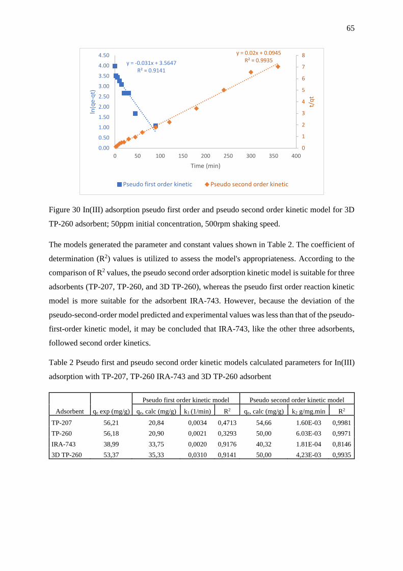
65
Figure 30 In(III) adsorption pseudo first order and pseudo second order kinetic model for 3D
TP-260 adsorbent; 50ppm initial concentration, 500rpm shaking speed.
The models generated the parameter and constant values shown in Table 2. The coefficient of
determination (R2) values is utilized to assess the model's appropriateness. According to the
comparison of R2 values, the pseudo second order adsorption kinetic model is suitable for three
adsorbents (TP-207, TP-260, and 3D TP-260), whereas the pseudo first order reaction kinetic
model is more suitable for the adsorbent IRA-743. However, because the deviation of the
pseudo-second-order model predicted and experimental values was less than that of the pseudo-
first-order kinetic model, it may be concluded that IRA-743, like the other three adsorbents,
followed second order kinetics.
Table 2 Pseudo first and pseudo second order kinetic models calculated parameters for In(III)
adsorption with TP-207, TP-260 IRA-743 and 3D TP-260 adsorbent
Adsorbent qe exp (mg/g)
Pseudo first order kinetic model Pseudo second order kinetic model
qe, calc (mg/g) k1 (1/min) R2 qe, calc (mg/g) k2 g/mg.min R2
TP-207 56,21 20,84 0,0034 0,4713 54,66 1.60E-03 0,9981
TP-260 56,18 20,90 0,0021 0,3293 50,00 6.03E-03 0,9971
IRA-743 38,99 33,75 0,0020 0,9176 40,32 1.81E-04 0,8146
3D TP-260 53,37 35,33 0,0310 0,9141 50,00 4,23E-03 0,9935
y = -0.031x + 3.5647R² = 0.9141
y = 0.02x + 0.0945R² = 0.9935
0
1
2
3
4
5
6
7
8
0.00
0.50
1.00
1.50
2.00
2.50
3.00
3.50
4.00
4.50
0 50 100 150 200 250 300 350 400
t/q
t
ln(q
e-q
t)
Time (min)
Pseudo first order kinetic Pseudo second order kinetic
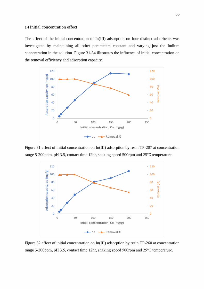
66
8.4 Initial concentration effect
The effect of the initial concentration of In(III) adsorption on four distinct adsorbents was
investigated by maintaining all other parameters constant and varying just the Indium
concentration in the solution. Figure 31-34 illustrates the influence of initial concentration on
the removal efficiency and adsorption capacity.
Figure 31 effect of initial concentration on In(III) adsorption by resin TP-207 at concentration
range 5-200ppm, pH 3.5, contact time 12hr, shaking speed 500rpm and 25℃ temperature.
Figure 32 effect of initial concentration on In(III) adsorption by resin TP-260 at concentration
range 5-200ppm, pH 3.5, contact time 12hr, shaking speed 500rpm and 25℃ temperature.
0
20
40
60
80
100
120
0
20
40
60
80
100
120
0 50 100 150 200 250
Rem
ova
l (%
)
Ad
sorp
tio
n c
apci
ty, q
e (m
g/g)
Initial concentration, Co (mg/g)
qe Removal %
0
20
40
60
80
100
120
0
20
40
60
80
100
120
0 50 100 150 200 250
Rem
ova
l (%
)
Ad
sorp
tio
n c
apci
ty, q
e (m
g/g)
Initial concentration, Co (mg/g)
qe Removal %
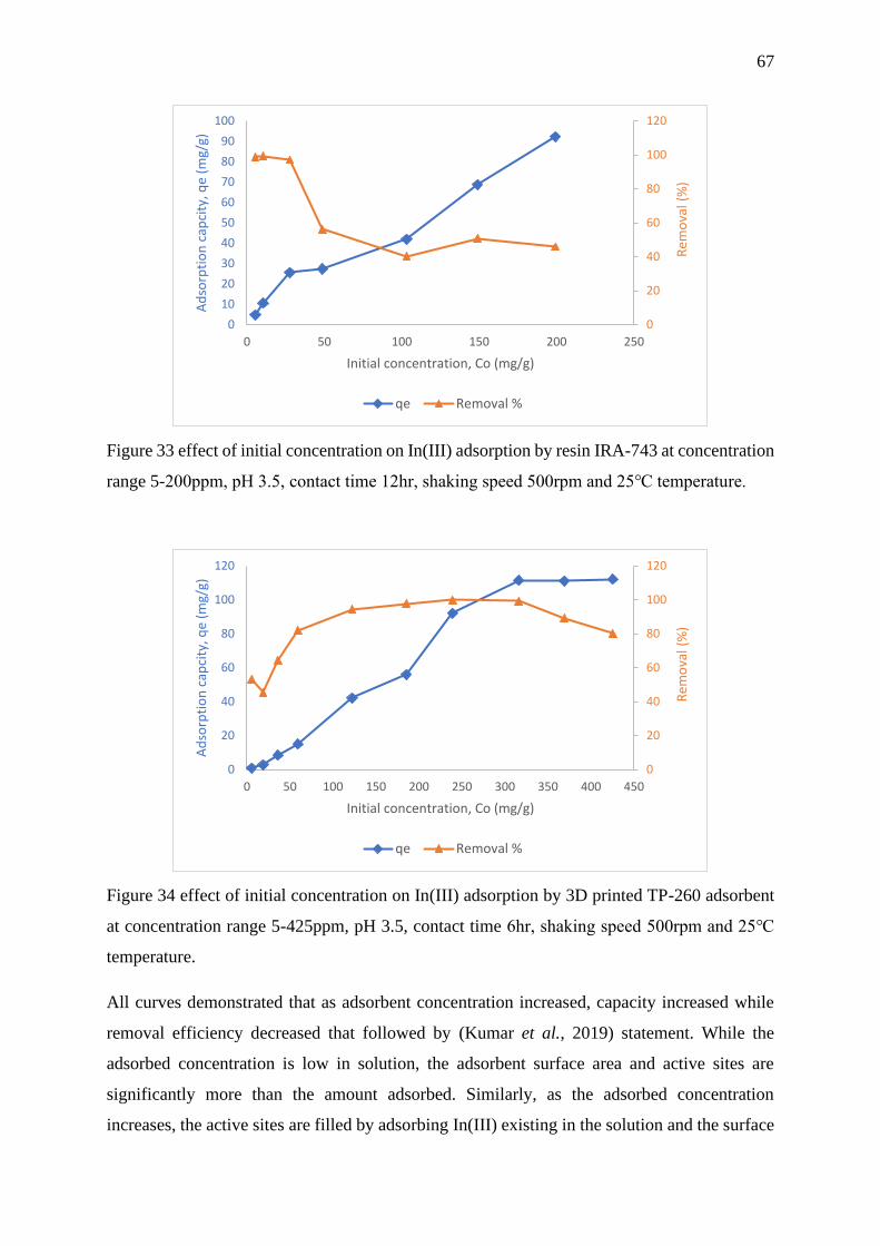
67
Figure 33 effect of initial concentration on In(III) adsorption by resin IRA-743 at concentration
range 5-200ppm, pH 3.5, contact time 12hr, shaking speed 500rpm and 25℃ temperature.
Figure 34 effect of initial concentration on In(III) adsorption by 3D printed TP-260 adsorbent
at concentration range 5-425ppm, pH 3.5, contact time 6hr, shaking speed 500rpm and 25℃
temperature.
All curves demonstrated that as adsorbent concentration increased, capacity increased while
removal efficiency decreased that followed by (Kumar et al., 2019) statement. While the
adsorbed concentration is low in solution, the adsorbent surface area and active sites are
significantly more than the amount adsorbed. Similarly, as the adsorbed concentration
increases, the active sites are filled by adsorbing In(III) existing in the solution and the surface
0
20
40
60
80
100
120
0
10
20
30
40
50
60
70
80
90
100
0 50 100 150 200 250
Rem
ova
l (%
)
Ad
sorp
tio
n c
apci
ty, q
e (m
g/g)
Initial concentration, Co (mg/g)
qe Removal %
0
20
40
60
80
100
120
0
20
40
60
80
100
120
0 50 100 150 200 250 300 350 400 450
Rem
ova
l (%
)
Ad
sorp
tio
n c
apci
ty, q
e (m
g/g)
Initial concentration, Co (mg/g)
qe Removal %
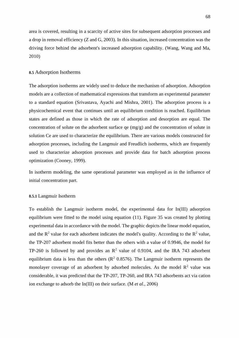
68
area is covered, resulting in a scarcity of active sites for subsequent adsorption processes and
a drop in removal efficiency (Z and G, 2003). In this situation, increased concentration was the
driving force behind the adsorbent's increased adsorption capability. (Wang, Wang and Ma,
2010)
8.5 Adsorption Isotherms
The adsorption isotherms are widely used to deduce the mechanism of adsorption. Adsorption
models are a collection of mathematical expressions that transform an experimental parameter
to a standard equation (Srivastava, Ayachi and Mishra, 2001). The adsorption process is a
physicochemical event that continues until an equilibrium condition is reached. Equilibrium
states are defined as those in which the rate of adsorption and desorption are equal. The
concentration of solute on the adsorbent surface qe (mg/g) and the concentration of solute in
solution Ce are used to characterize the equilibrium. There are various models constructed for
adsorption processes, including the Langmuir and Freudlich isotherms, which are frequently
used to characterize adsorption processes and provide data for batch adsorption process
optimization (Cooney, 1999).
In isotherm modeling, the same operational parameter was employed as in the influence of
initial concentration part.
8.5.1 Langmuir Isotherm
To establish the Langmuir isotherm model, the experimental data for In(III) adsorption
equilibrium were fitted to the model using equation (11). Figure 35 was created by plotting
experimental data in accordance with the model. The graphic depicts the linear model equation,
and the R2 value for each adsorbent indicates the model's quality. According to the R2 value,
the TP-207 adsorbent model fits better than the others with a value of 0.9946, the model for
TP-260 is followed by and provides an R2 value of 0.9104, and the IRA 743 adsorbent
equilibrium data is less than the others (R2 0.8576). The Langmuir isotherm represents the
monolayer coverage of an adsorbent by adsorbed molecules. As the model R2 value was
considerable, it was predicted that the TP-207, TP-260, and IRA 743 adsorbents act via cation
ion exchange to adsorb the In(III) on their surface. (M et al., 2006)
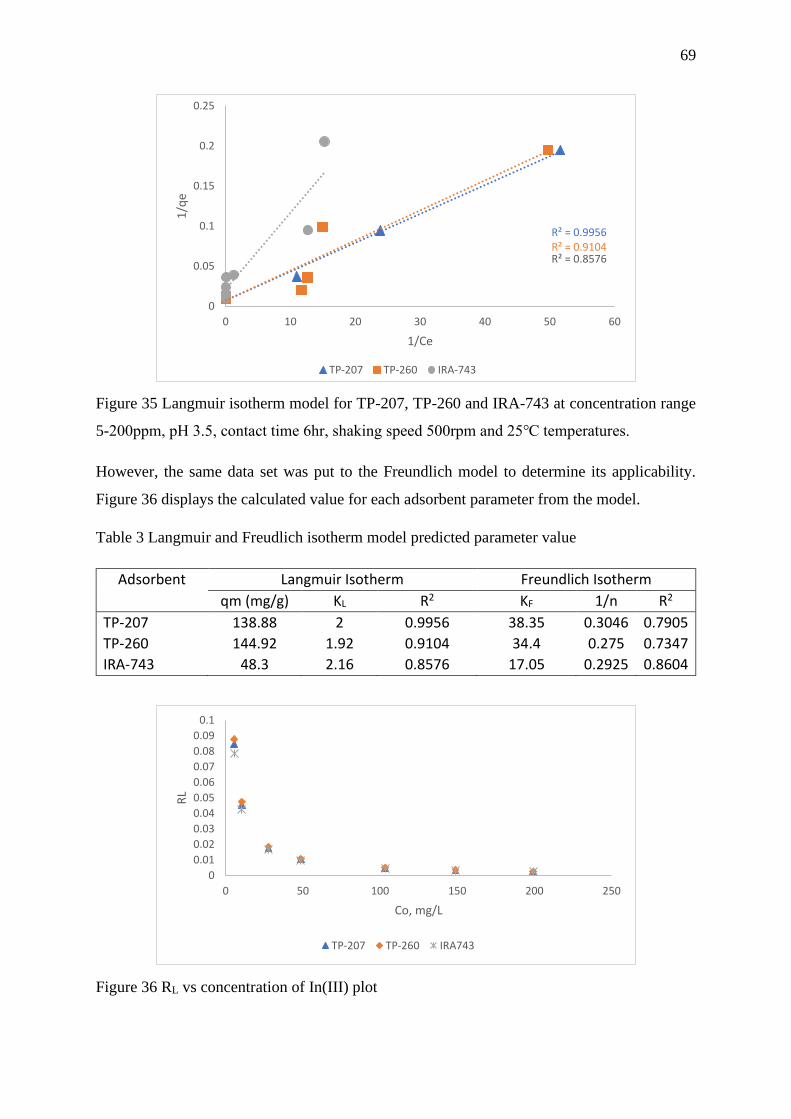
69
Figure 35 Langmuir isotherm model for TP-207, TP-260 and IRA-743 at concentration range
5-200ppm, pH 3.5, contact time 6hr, shaking speed 500rpm and 25℃ temperatures.
However, the same data set was put to the Freundlich model to determine its applicability.
Figure 36 displays the calculated value for each adsorbent parameter from the model.
Table 3 Langmuir and Freudlich isotherm model predicted parameter value
Adsorbent Langmuir Isotherm Freundlich Isotherm
qm (mg/g) KL R2 KF 1/n R2
TP-207 138.88 2 0.9956 38.35 0.3046 0.7905
TP-260 144.92 1.92 0.9104 34.4 0.275 0.7347
IRA-743 48.3 2.16 0.8576 17.05 0.2925 0.8604
Figure 36 RL vs concentration of In(III) plot
R² = 0.9956R² = 0.9104R² = 0.8576
0
0.05
0.1
0.15
0.2
0.25
0 10 20 30 40 50 60
1/q
e
1/Ce
TP-207 TP-260 IRA-743
0
0.01
0.02
0.03
0.04
0.05
0.06
0.07
0.08
0.09
0.1
0 50 100 150 200 250
RL
Co, mg/L
TP-207 TP-260 IRA743
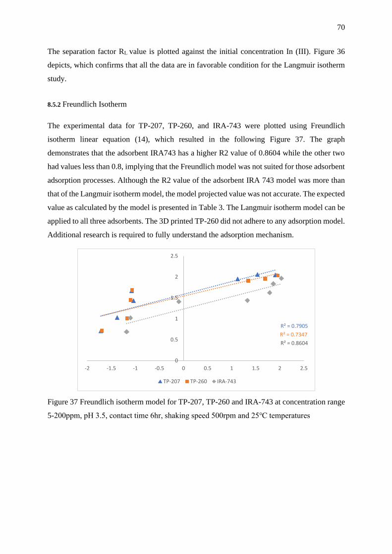
70
The separation factor RL value is plotted against the initial concentration In (III). Figure 36
depicts, which confirms that all the data are in favorable condition for the Langmuir isotherm
study.
8.5.2 Freundlich Isotherm
The experimental data for TP-207, TP-260, and IRA-743 were plotted using Freundlich
isotherm linear equation (14), which resulted in the following Figure 37. The graph
demonstrates that the adsorbent IRA743 has a higher R2 value of 0.8604 while the other two
had values less than 0.8, implying that the Freundlich model was not suited for those adsorbent
adsorption processes. Although the R2 value of the adsorbent IRA 743 model was more than
that of the Langmuir isotherm model, the model projected value was not accurate. The expected
value as calculated by the model is presented in Table 3. The Langmuir isotherm model can be
applied to all three adsorbents. The 3D printed TP-260 did not adhere to any adsorption model.
Additional research is required to fully understand the adsorption mechanism.
Figure 37 Freundlich isotherm model for TP-207, TP-260 and IRA-743 at concentration range
5-200ppm, pH 3.5, contact time 6hr, shaking speed 500rpm and 25℃ temperatures
R² = 0.7905
R² = 0.7347
R² = 0.8604
0
0.5
1
1.5
2
2.5
-2 -1.5 -1 -0.5 0 0.5 1 1.5 2 2.5
TP-207 TP-260 IRA-743
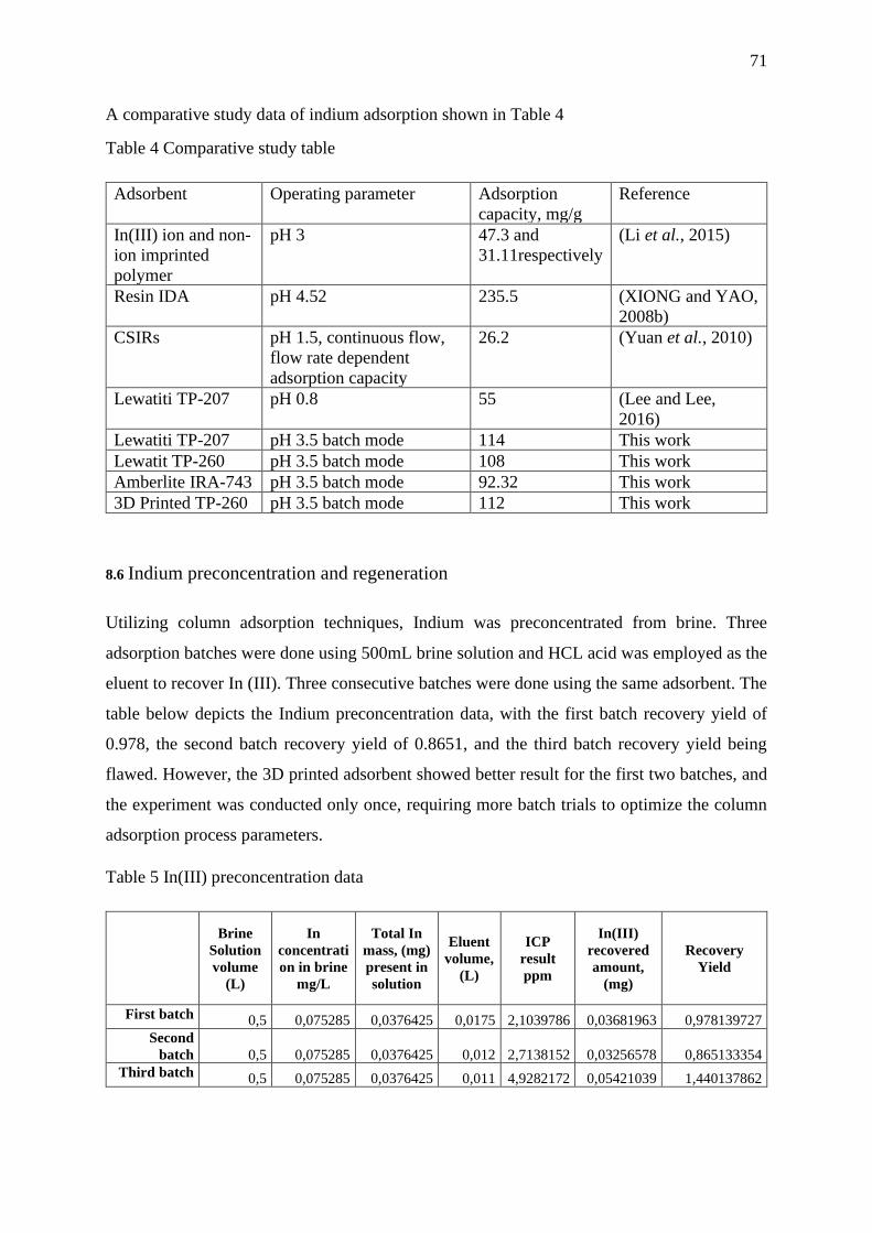
71
A comparative study data of indium adsorption shown in Table 4
Table 4 Comparative study table
Adsorbent Operating parameter Adsorption
capacity, mg/g
Reference
In(III) ion and non-
ion imprinted
polymer
pH 3 47.3 and
31.11respectively
(Li et al., 2015)
Resin IDA pH 4.52 235.5 (XIONG and YAO,
2008b)
CSIRs pH 1.5, continuous flow,
flow rate dependent
adsorption capacity
26.2 (Yuan et al., 2010)
Lewatiti TP-207 pH 0.8 55 (Lee and Lee,
2016)
Lewatiti TP-207 pH 3.5 batch mode 114 This work
Lewatit TP-260 pH 3.5 batch mode 108 This work
Amberlite IRA-743 pH 3.5 batch mode 92.32 This work
3D Printed TP-260 pH 3.5 batch mode 112 This work
8.6 Indium preconcentration and regeneration
Utilizing column adsorption techniques, Indium was preconcentrated from brine. Three
adsorption batches were done using 500mL brine solution and HCL acid was employed as the
eluent to recover In (III). Three consecutive batches were done using the same adsorbent. The
table below depicts the Indium preconcentration data, with the first batch recovery yield of
0.978, the second batch recovery yield of 0.8651, and the third batch recovery yield being
flawed. However, the 3D printed adsorbent showed better result for the first two batches, and
the experiment was conducted only once, requiring more batch trials to optimize the column
adsorption process parameters.
Table 5 In(III) preconcentration data
Brine
Solution
volume
(L)
In
concentrati
on in brine
mg/L
Total In
mass, (mg)
present in
solution
Eluent
volume,
(L)
ICP
result
ppm
In(III)
recovered
amount,
(mg)
Recovery
Yield
First batch 0,5 0,075285 0,0376425 0,0175 2,1039786 0,03681963 0,978139727
Second
batch 0,5 0,075285 0,0376425 0,012 2,7138152 0,03256578 0,865133354
Third batch 0,5 0,075285 0,0376425 0,011 4,9282172 0,05421039 1,440137862
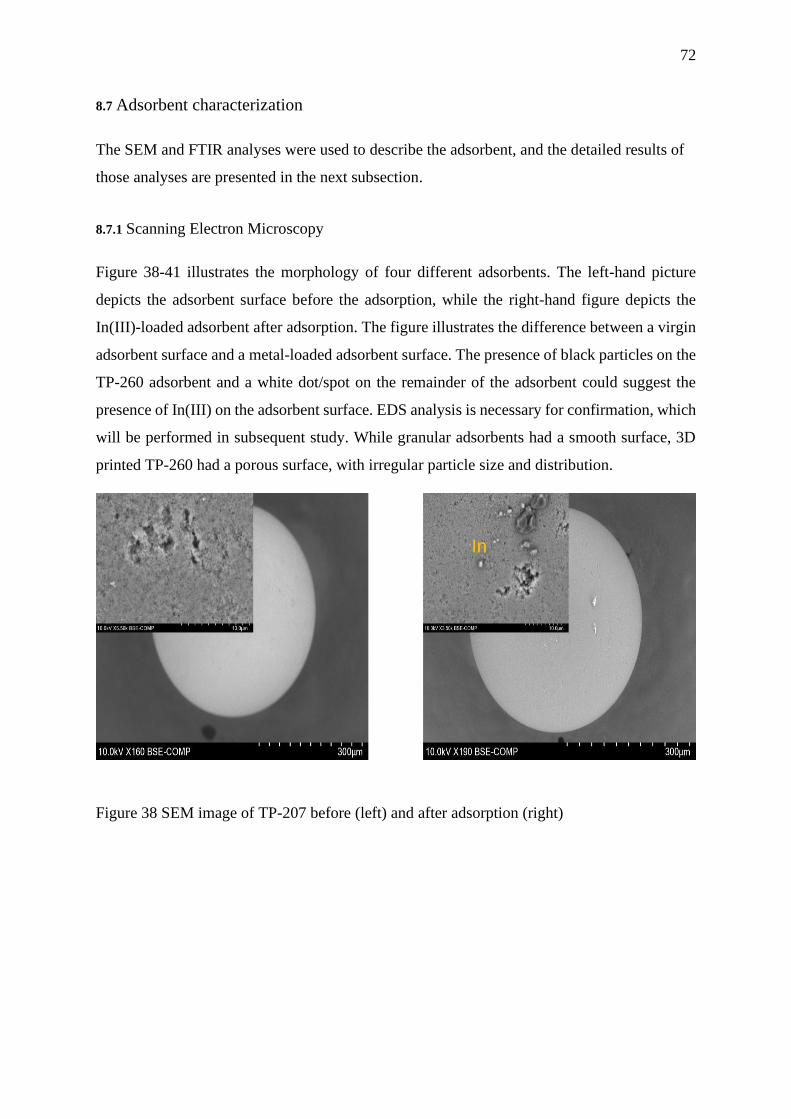
72
8.7 Adsorbent characterization
The SEM and FTIR analyses were used to describe the adsorbent, and the detailed results of
those analyses are presented in the next subsection.
8.7.1 Scanning Electron Microscopy
Figure 38-41 illustrates the morphology of four different adsorbents. The left-hand picture
depicts the adsorbent surface before the adsorption, while the right-hand figure depicts the
In(III)-loaded adsorbent after adsorption. The figure illustrates the difference between a virgin
adsorbent surface and a metal-loaded adsorbent surface. The presence of black particles on the
TP-260 adsorbent and a white dot/spot on the remainder of the adsorbent could suggest the
presence of In(III) on the adsorbent surface. EDS analysis is necessary for confirmation, which
will be performed in subsequent study. While granular adsorbents had a smooth surface, 3D
printed TP-260 had a porous surface, with irregular particle size and distribution.
Figure 38 SEM image of TP-207 before (left) and after adsorption (right)
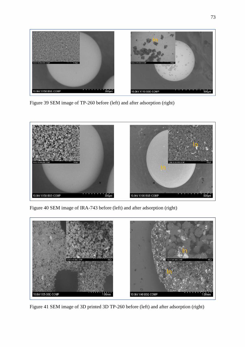
73
Figure 39 SEM image of TP-260 before (left) and after adsorption (right)
Figure 40 SEM image of IRA-743 before (left) and after adsorption (right)
Figure 41 SEM image of 3D printed 3D TP-260 before (left) and after adsorption (right)
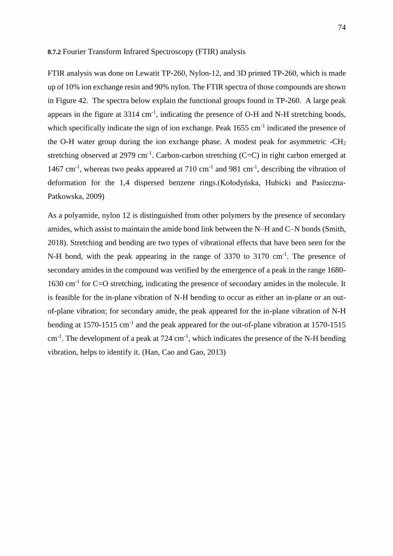
74
8.7.2 Fourier Transform Infrared Spectroscopy (FTIR) analysis
FTIR analysis was done on Lewatit TP-260, Nylon-12, and 3D printed TP-260, which is made
up of 10% ion exchange resin and 90% nylon. The FTIR spectra of those compounds are shown
in Figure 42. The spectra below explain the functional groups found in TP-260. A large peak
appears in the figure at 3314 cm-1, indicating the presence of O-H and N-H stretching bonds,
which specifically indicate the sign of ion exchange. Peak 1655 cm-1 indicated the presence of
the O-H water group during the ion exchange phase. A modest peak for asymmetric -CH2
stretching observed at 2979 cm-1. Carbon-carbon stretching (C=C) in right carbon emerged at
1467 cm-1, whereas two peaks appeared at 710 cm-1 and 981 cm-1, describing the vibration of
deformation for the 1,4 dispersed benzene rings.(Kołodyńska, Hubicki and Pasieczna-
Patkowska, 2009)
As a polyamide, nylon 12 is distinguished from other polymers by the presence of secondary
amides, which assist to maintain the amide bond link between the N–H and C–N bonds (Smith,
2018). Stretching and bending are two types of vibrational effects that have been seen for the
N-H bond, with the peak appearing in the range of 3370 to 3170 cm-1. The presence of
secondary amides in the compound was verified by the emergence of a peak in the range 1680-
1630 cm-1 for C=O stretching, indicating the presence of secondary amides in the molecule. It
is feasible for the in-plane vibration of N-H bending to occur as either an in-plane or an out-
of-plane vibration; for secondary amide, the peak appeared for the in-plane vibration of N-H
bending at 1570-1515 cm-1 and the peak appeared for the out-of-plane vibration at 1570-1515
cm-1. The development of a peak at 724 cm-1, which indicates the presence of the N-H bending
vibration, helps to identify it. (Han, Cao and Gao, 2013)
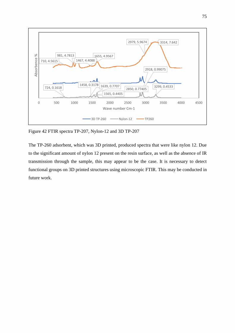
75
Figure 42 FTIR spectra TP-207, Nylon-12 and 3D TP-207
The TP-260 adsorbent, which was 3D printed, produced spectra that were like nylon 12. Due
to the significant amount of nylon 12 present on the resin surface, as well as the absence of IR
transmission through the sample, this may appear to be the case. It is necessary to detect
functional groups on 3D printed structures using microscopic FTIR. This may be conducted in
future work.
3299, 0.4533
2918, 0.99075
2850, 0.774051639, 0.7707
1565, 0.4405
1458, 0.3178724, 0.1618
3314, 7.6422979, 5.9674
1655, 4.95671467, 4.4088
981, 4.7813
710, 4.5615
0 500 1000 1500 2000 2500 3000 3500 4000 4500
Ab
sorb
ence
%
Wave number Cm-1
3D TP-260 Nylon-12 TP260
76
9. Conclusions
The goal of this thesis study was to develop technologies for recovering Indium from seawater
brine solutions via adsorption. The entire study can be divided into three parts: first, three
commercial resins were used in regular form to observe adsorptive behavior for Indium;
second, the experimental analysis data were evaluated, and suitable Indium adsorption
functional resin figure out and taken resin for AM manufacturing process; in the last phase, an
additively produced adsorbent was subjected to batch adsorption using Indium standard
solution and column adsorption tests in order to accomplish Indium preconcentrating using
brine solution.
This study was employed to the following commercial resins: Lewatit TP-207 iminodiacetic
acid-based cation exchange resin, Lewatit TP-260 phosphonic acid-based cation exchange
resin, and Amberlite IRA-743 chelating cation exchange resin. In the kinetic behavior analysis,
TP-260 had a higher adsorption capacity for a shorter period than the other two resins, with a
maximum adsorption capacity of 56 mg/g at 240 minutes. Based on this finding, the TP-260
resin was chosen for 3D printed adsorbent manufacture, with 10% resin and 90% nylon 12
employed as raw materials. The batch adsorption experiment was carried out utilizing 3D
printed TP-260 and yielded about the same adsorption capacity as general formed resin TP-
260. At 120 minutes, the maximum adsorption capacity of 3D printed TP 260 was 52mg/g.
This finding is quite surprising, because the results could worsen owing to the ion exchange
resin active site capping by the nylon 12 materials because there is no strong evidence that
nylon 12 materials have functionality for Indium adsorption.
The kinetic analysis revealed that all the adsorbents used in this study followed pseudo second
order reaction kinetic, which was assessed using the R2 value and model predicted value
variation. Although the adsorbent IRA-743 had a greater value for the pseudo first order
kinetic, the second order model projected value was more accurate than the pseudo first order
kinetic.
On the equilibrium experimental data of each adsorbent, the Langmuir and Freundlich isotherm
models were used, and it seems that three ion exchange resins followed the Langmuir isotherm,
indicating monolayer adsorption of In(III) on the adsorbent surface. The experimental data
77
appropriateness for those three adsorbents was also verified, and all data were determined to
be beneficial for Indium adsorption. The 3D printed TP-260, on the other hand, did not adhere
to any isotherm model. It may occur as a result of the adsorbent's heterogeneous surface and
multi-layer adsorption. More research is needed to determine the true cause of this.
To preconcentrate Indium from brine solution, column-based adsorption was used. In this
experiment, the first two batches provided significant Indium recovery yield (1st batch: 0,978
and 2nd batch: 0,8651), whereas the third batch experiment was reported as flawed. Further
trials are required to optimize process parameters, eluent acid concentration, and the structure
of the 3D printed adsorbent.
A few recommendations for future work are enlisted below:
• Indium selective adsorbent has not been tested yet. That is required to be done in the
future.
• EDS analysis is required to confirm the presence of Indium on the adsorbent surface.
• Zeta potential analysis may be used to characterize the adsorbent.
• Optimization of column adsorption parameters and 3D-printed adsorbent design
• Characterize the column adsorption mechanism.
• Due to a lack of IR rays passing through the sample in conventional FTIR instruments,
the microscopic FTIR analysis necessary to identify the surface functional group as a
3D printed component did not produce a meaningful result for the 3D manufactured
adsorbent.
78
10. References
Akama, Y., Suzuki, S. and Monobe, Y. (2016) “STUDY ON THE ADSORPTION AND
SELECTIVE SEPARATION OF INDIUM FROM ZINC WITH CHELATING
CELLULOSE,” CELLULOSE CHEMISTRY AND TECHNOLOGY Cellulose Chem. Technol,
50(1), pp. 147–152.
Alfantazi, A.M.; Moskalyk, R.R. (2003) “Processing of Indium: a review,” Mineral
Engineering, 16(8), pp. 687–694. doi:10.1016/S0892-6875(03)00168-7.
Alguacil, F.J. et al. (2016) “Sorption of indium (III) onto carbon nanotubes,” Ecotoxicology
and Environmental Safety, 130. doi:10.1016/j.ecoenv.2016.04.008.
Amakawa, H., Alibo, D.S. and Nozaki, Y. (1996) “Indium concentration in Pacific seawater,”
Geophysical Research Letters, 23(18), pp. 2473–2476. doi:10.1029/96GL02300.
Argenta, A.B. et al. (2017) “Supercritical CO2 extraction of indium present in liquid crystal
displays from discarded cell phones using organic acids,” The Journal of Supercritical
Fluids, 120, pp. 95–101. doi:10.1016/J.SUPFLU.2016.10.014.
Assefi, M. et al. (2018a) “Selective recovery of indium from scrap LCD panels using
macroporous resins,” Journal of Cleaner Production, 180, pp. 814–822.
doi:10.1016/J.JCLEPRO.2018.01.165.
Assefi, M. et al. (2018b) “Selective recovery of indium from scrap LCD panels using
macroporous resins,” Journal of Cleaner Production, 180, pp. 814–822.
doi:10.1016/J.JCLEPRO.2018.01.165.
B, C. et al. (2011) “Synthesis of hierarchical Ni(OH)(2) and NiO nanosheets and their
adsorption kinetics and isotherms to Congo red in water,” Journal of hazardous materials,
185(2–3), pp. 889–897. doi:10.1016/J.JHAZMAT.2010.09.104.
B, S. et al. (2016a) “Beneficiation and recovery of indium from liquid-crystal-display glass
by hydrometallurgy,” Waste management (New York, N.Y.), 57, pp. 207–214.
doi:10.1016/J.WASMAN.2016.02.019.
B, S. et al. (2016b) “Beneficiation and recovery of indium from liquid-crystal-display glass
by hydrometallurgy,” Waste management (New York, N.Y.), 57, pp. 207–214.
doi:10.1016/J.WASMAN.2016.02.019.
Balla, V.K., Bose, S. and Bandyopadhyay, A. (2008) “Processing of Bulk Alumina Ceramics
Using Laser Engineered Net Shaping,” International Journal of Applied Ceramic
Technology, 5(3), pp. 234–242. doi:10.1111/J.1744-7402.2008.02202.X.
Binder Jetting | Additive Manufacturing Research Group | Loughborough University (no
date). Available at:
https://www.lboro.ac.uk/research/amrg/about/the7categoriesofadditivemanufacturing/binderj
etting/ (Accessed: August 27, 2021).
79
Bolt, G.H. and van Olphen, H. (1985) “The Surface Chemistry of Soils,” Clays and Clay
Minerals 1985 33:4, 33(4), pp. 367–367. doi:10.1346/CCMN.1985.0330415.
Caulfield, B., McHugh, P.E. and Lohfeld, S. (2007) “Dependence of mechanical properties of
polyamide components on build parameters in the SLS process,” Journal of Materials
Processing Technology, 182(1–3), pp. 477–488. doi:10.1016/J.JMATPROTEC.2006.09.007.
Chang, J. et al. (2016) “Separation of indium from iron in a rotating packed bed contactor
using Di-2-ethylhexylphosphoric acid,” Separation and Purification Technology, 164, pp.
12–18. doi:10.1016/J.SEPPUR.2016.03.017.
Chow, T.J. and Snyder, C.B. (1969) “Indium content of sea water,” Earth and Planetary
Science Letters, 7(3), pp. 221–223. doi:10.1016/0012-821X(69)90054-5.
Cooney, D.O. (1999) “Adsorption design for wastewater treatment,” p. 190.
Criales, L.E. et al. (2017) “Laser powder bed fusion of nickel alloy 625: Experimental
investigations of effects of process parameters on melt pool size and shape with spatter
analysis,” International Journal of Machine Tools and Manufacture, 121, pp. 22–36.
doi:10.1016/J.IJMACHTOOLS.2017.03.004.
Crundwell, F.K. (1988) “Effect of iron impurity in zinc sulfide concentrates on the rate of
dissolution,” AIChE Journal, 34(7), pp. 1128–1134. doi:10.1002/AIC.690340709.
D, F. et al. (2015) “Materials recovery from waste liquid crystal displays: A focus on
indium,” Waste management (New York, N.Y.), 45, pp. 325–333.
doi:10.1016/J.WASMAN.2015.07.043.
Deckers, J., Vleugels, J. and Kruth, J.P. (2014) “Additive manufacturing of ceramics: A
review,” Journal of Ceramic Science and Technology, 5(4), pp. 245–260.
doi:10.4416/JCST2014-00032.
Deferm, C. et al. (2017) “Speciation of indium(iii) chloro complexes in the solvent extraction
process from chloride aqueous solutions to ionic liquids,” Dalton Transactions, 46(13).
doi:10.1039/c7dt00618g.
Downs, A.J. (1993) Chemistry of Aluminium, Gallium, Indium and Thallium. First Edit.
F, F. et al. (2017) “Separation and recovery of glass, plastic and indium from spent LCD
panels,” Waste management (New York, N.Y.), 60, pp. 569–581.
doi:10.1016/J.WASMAN.2016.12.030.
Feng, L., Wang, Y. and Wei, Q. (2019) “PA12 Powder Recycled from SLS for FDM,”
Polymers 2019, Vol. 11, Page 727, 11(4), p. 727. doi:10.3390/POLYM11040727.
Filippou, D. and Demopoulos, G.P. (1997) “Steady-state modeling of zinc-ferrite hot-acid
leaching,” Metallurgical and Materials Transactions B 1997 28:4, 28(4), pp. 701–711.
doi:10.1007/S11663-997-0044-0.
Foo, K.Y. and Hameed, B.H. (2010) “Insights into the modeling of adsorption isotherm
systems,” Chemical Engineering Journal, 156(1), pp. 2–10. doi:10.1016/J.CEJ.2009.09.013.
80
Fortes, M. C.B., Martins, A.H. and Benedetto, J.S. (2007) “Selective separation of indium by
iminodiacetic acid chelating resin,” Brazilian Journal of Chemical Engineering, 24(2), pp.
287–292. doi:10.1590/S0104-66322007000200013.
Fortes, M. C. B., Martins, A.H. and Benedetto, J.S. (2007) “Selective separation of indium by
iminodiacetic acid chelating resin,” Brazilian Journal of Chemical Engineering, 24(2), pp.
287–292. doi:10.1590/S0104-66322007000200013.
French, S.J. (1934) “A story of indium,” Journal of Chemical Education, 11(5), p. 270.
doi:10.1021/ed011p270.
Frenzel, Max; Mikolajczak, Claire; Reuter, Markus A.; Gutzmer, J. (2017) “Quantifying the
relative availability of high-tech by-product metals – The cases of gallium, germanium and
indium,” Resource Policy, 52, pp. 327–335. doi:10.1016/j.resourpol.2017.04.008.
Frenzel, Max; Tolosana-Delgado, Raimon; Gutzmer, J. (2015) “Assessing the supply
potential of high-tech metals – A general method",” Resource Policy, 46(part 2), pp. 45–58.
doi:10.1016/j.resourpol.2015.08.002.
Ghoreishi, S.M., Ansari, K. and Ghaziaskar, H.S. (2012) “Supercritical extraction of toxic
heavy metals from aqueous waste via Cyanex 301 as chelating agent,” The Journal of
Supercritical Fluids, 72, pp. 288–297. doi:10.1016/J.SUPFLU.2012.10.003.
Gibson, I., Rosen, D.W. and Stucker, B. (2010) “Additive manufacturing technologies: Rapid
prototyping to direct digital manufacturing,” Additive Manufacturing Technologies: Rapid
Prototyping to Direct Digital Manufacturing, pp. 1–459. doi:10.1007/978-1-4419-1120-9.
Giles, C.H., Smith, D. and Huitson, A. (1974) “A general treatment and classification of the
solute adsorption isotherm. I. Theoretical,” Journal of Colloid and Interface Science, 47(3),
pp. 755–765. doi:10.1016/0021-9797(74)90252-5.
Greenwood, N.N.; Earnshaw, A. (1997) Chemistry of the Elements. Second Edi. Pergamon
Press plc.
Grimes, S.M., Yasri, N.G. and Chaudhary, A.J. (2017) “Recovery of critical metals from
dilute leach solutions – Separation of indium from tin and lead,” Inorganica Chimica Acta,
461, pp. 161–166. doi:10.1016/J.ICA.2017.02.002.
H, Y., M, T. and Y, T. (1999) “Production of organic acids and amino acids from fish meat
by sub-critical water hydrolysis,” Biotechnology progress, 15(6), pp. 1090–1094.
doi:10.1021/BP9900920.
Han, J., Cao, Z. and Gao, W. (2013) “Remarkable sorption properties of polyamide 12
microspheres for a broad-spectrum antibacterial (triclosan) in water,” Journal of Materials
Chemistry A, 1(16), pp. 4941–4944. doi:10.1039/C3TA00090G.
Hanna, O. T., Sandall, O.C. (1995) “Computational Method in Chemical Engineering,”
Englewood Cliffs, NJ: Prentice-Hall International, pp. 127–130.
Hasegawa, H. et al. (2013) “Selective recovery of indium from the etching waste solution of
the flat-panel display fabrication process,” Microchemical Journal, 110, pp. 133–139.
doi:10.1016/J.MICROC.2013.03.005.
81
Haynes, W.M, Lide, D.R. (2010) CRC Handbook of Chemistry and Physics: A ready
reference book of Chemical and Physical Data.
Hinz, C. (2001) “Description of sorption data with isotherm equations,” Geoderma, 99(3–4),
pp. 225–243. doi:10.1016/S0016-7061(00)00071-9.
Ho, H.C.H., Gibson, I. and Cheung, W.L. (1999) “Effects of energy density on morphology
and properties of selective laser sintered polycarbonate,” Journal of Materials Processing
Technology, 89–90, pp. 204–210. doi:10.1016/S0924-0136(99)00007-2.
Ho, Y.S. and McKay, G. (1999) “Pseudo-second order model for sorption processes,”
Process Biochemistry, 34(5), pp. 451–465. doi:10.1016/S0032-9592(98)00112-5.
Hofland, E.C., Baran, I. and Wismeijer, D.A. (2017) “Correlation of Process Parameters with
Mechanical Properties of Laser Sintered PA12 Parts,” Advances in Materials Science and
Engineering, 2017. doi:10.1155/2017/4953173.
Hsieh, S.-J., Chen, C.-C. and Say, W.C. (2009) “Process for recovery of indium from ITO
scraps and metallurgic microstructures,” Materials Science & Engineering B, 1–3(158), pp.
82–87. doi:10.1016/J.MSEB.2009.01.019.
J, L. et al. (2009) “Recovery of valuable materials from waste liquid crystal display panel,”
Waste management (New York, N.Y.), 29(7), pp. 2033–2039.
doi:10.1016/J.WASMAN.2008.12.013.
Jeon, C., Cha, J.H. and Choi, J.Y. (2015) “Adsorption and recovery characteristics of
phosphorylated sawdust bead for indium(III) in industrial wastewater,” Journal of Industrial
and Engineering Chemistry, 27, pp. 201–206. doi:10.1016/J.JIEC.2014.12.036.
Jiang, J., Liang, D. and Zhong, Q. (2011) “Precipitation of indium using sodium
tripolyphosphate,” Hydrometallurgy, 106(3–4), pp. 165–169.
doi:10.1016/J.HYDROMET.2010.12.009.
Kapoor, A. and Yang, R.T. (1989) “Correlation of equilibrium adsorption data of condensible
vapours on porous adsorbents,” Gas Separation & Purification, 3(4), pp. 187–192.
doi:10.1016/0950-4214(89)80004-0.
Kato, T. et al. (2013) “Separation and concentration of indium from a liquid crystal display
via homogeneous liquid–liquid extraction,” Hydrometallurgy, Complete(137), pp. 148–155.
doi:10.1016/J.HYDROMET.2013.06.004.
Kaukinen, A., Sc, D. and Virolainen, S. (no date) “Ion exchange in hydrometallurgical
recycling of Li-ion battery metals: production of Li-Ni-Co mixture Examiners: Professor
Tuomo Sainio.”
Kołodyńska, D., Hubicki, Z. and Pasieczna-Patkowska, S. (2009) “FT-ir/pas studies of cu(II)-
EDTA complexes sorption on the chelating ion exchangers,” Acta Physica Polonica A,
116(3), pp. 340–343. doi:10.12693/APHYSPOLA.116.340.
Kumar, M. et al. (2019) “Valorization of coal fired-fly ash for potential heavy metal removal
from the single and multi-contaminated system,” Heliyon, 5(10), p. e02562.
doi:10.1016/J.HELIYON.2019.E02562.
82
Kumar, S. (2020) “Introduction of Additive Manufacturing Processes,” Additive
Manufacturing Processes, pp. 1–19. doi:10.1007/978-3-030-45089-2_1.
Kundu, S. and Gupta, A.K. (2006) “Arsenic adsorption onto iron oxide-coated cement
(IOCC): Regression analysis of equilibrium data with several isotherm models and their
optimization,” Chemical Engineering Journal, 122(1–2), pp. 93–106.
doi:10.1016/J.CEJ.2006.06.002.
Lahtinen, E. et al. (2017) “Selective Recovery of Gold from Electronic Waste Using 3D-
Printed Scavenger,” ACS Omega, 2(10), pp. 7299–7304. doi:10.1021/acsomega.7b01215.
Lahtinen, E. et al. (2018) “Porous 3D Printed Scavenger Filters for Selective Recovery of
Precious Metals from Electronic Waste,” Advanced Sustainable Systems, 2(10).
doi:10.1002/adsu.201800048.
Lahtinen, E. et al. (2019) “Selective Laser Sintering of Metal-Organic Frameworks:
Production of Highly Porous Filters by 3D Printing onto a Polymeric Matrix,”
ChemPlusChem, 84(2), pp. 222–225. doi:10.1002/cplu.201900081.
Langmuir, I. (2002) “THE ADSORPTION OF GASES ON PLANE SURFACES OF
GLASS, MICA AND PLATINUM.,” Journal of the American Chemical Society, 40(9), pp.
1361–1403. doi:10.1021/JA02242A004.
Lee, S.K. and Lee, U.H. (2016) “Adsorption and desorption property of iminodiacetate resin
(Lewatit® TP207) for indium recovery,” Journal of Industrial and Engineering Chemistry,
40, pp. 23–25. doi:10.1016/J.JIEC.2016.05.016.
Lewatit-Lenntech (no date) “Lewatit-MonoPlus-TP-260-Resin-Lenntech.”
Li, C. et al. (2010) “Oxidative pressure leaching of sphalerite concentrate with high indium
and iron content in sulfuric acid medium,” Hydrometallurgy, 102(1–4), pp. 91–94.
doi:10.1016/J.HYDROMET.2010.01.009.
Li, F. et al. (2018) “High efficient separation of U(VI) and Th(IV) from rare earth elements
in strong acidic solution by selective sorption on phenanthroline diamide functionalized
graphene oxide,” Chemical Engineering Journal, 332. doi:10.1016/j.cej.2017.09.038.
Li, H. et al. (2012) “Adsorption behavior of indium(III) on modified solvent impregnated
resins (MSIRs) containing sec-octylphenoxy acetic acid,” Hydrometallurgy, 121–124, pp.
60–67. doi:10.1016/J.HYDROMET.2012.04.005.
Li, M. et al. (2018) “A novel In(III) ion-imprinted polymer (IIP) for selective extraction of
In(III) ions from aqueous solutions,” Hydrometallurgy, 176.
doi:10.1016/j.hydromet.2018.02.006.
Li, Min et al. (2015) “Synthesis and application of a surface-grafted In (III) ion-imprinted
polymer for selective separation and pre-concentration of indium (III) ion from aqueous
solution,” Hydrometallurgy, Complete(154), pp. 63–71.
doi:10.1016/J.HYDROMET.2015.03.011.
83
Li, R. Di et al. (2014a) “Recovery of indium by acid leaching waste ITO target based on
neural network,” Transactions of Nonferrous Metals Society of China, 24(1), pp. 257–262.
doi:10.1016/S1003-6326(14)63055-7.
Li, R. Di et al. (2014b) “Recovery of indium by acid leaching waste ITO target based on
neural network,” Transactions of Nonferrous Metals Society of China, 24(1), pp. 257–262.
doi:10.1016/S1003-6326(14)63055-7.
Li, X.-H. et al. (2010) “Indium recovery from zinc oxide flue dust by oxidative pressure
leaching,” Trans. Nonferrous Met. Soc. China, 20, pp. 141–145.
Li, Y. et al. (2011) “Recovery of indium from used indium–tin oxide (ITO) targets,”
Hydrometallurgy, 105(3–4), pp. 207–212. doi:10.1016/J.HYDROMET.2010.09.006.
Liu, L. et al. (2019) “Application of Nanotechnology in the Removal of Heavy Metal From
Water,” Nanomaterials for the Removal of Pollutants and Resource Reutilization, pp. 83–
147. doi:10.1016/B978-0-12-814837-2.00004-4.
Lokanc, M., Eggert, R. and Redlinger, M. (2015) “The Availability of Indium: The Present,
Medium Term, and Long Term.” doi:10.2172/1327212.
M, N. et al. (2006) “Sorption of lead from aqueous solution by chemically modified carbon
adsorbents,” Journal of hazardous materials, 138(3), pp. 604–613.
doi:10.1016/J.JHAZMAT.2006.05.098.
Malek A., Farooq, S. (1996) “Comparison of isotherm models for hydrocarbon on activated
carbon,” The American Institute of Chemical Engineers Journal, 42(11), pp. 3191–3201.
Mane, V.S., Deo Mall, I. and Chandra Srivastava, V. (2007) “Kinetic and equilibrium
isotherm studies for the adsorptive removal of Brilliant Green dye from aqueous solution by
rice husk ash,” Journal of Environmental Management, 84(4), pp. 390–400.
doi:10.1016/J.JENVMAN.2006.06.024.
Marquardt, D.W. (2006) “An Algorithm for Least-Squares Estimation of Nonlinear
Parameters,” http://dx.doi.org/10.1137/0111030, 11(2), pp. 431–441. doi:10.1137/0111030.
Material Extrusion | Additive Manufacturing Research Group | Loughborough University (no
date). Available at:
https://www.lboro.ac.uk/research/amrg/about/the7categoriesofadditivemanufacturing/materia
lextrusion/ (Accessed: August 27, 2021).
MATTHEWS, A.D. and RILEY, J.P. (1970) “Occurrence of Indium in Seawater and some
Marine Sediments,” Nature 1970 225:5239, 225(5239), pp. 1242–1242.
doi:10.1038/2251242a0.
Myers, R.H. (1990) “Classical and Modern Regression with Applications,” PWS-KENT,
29(4), pp. 691–693.
Ng, J.C.Y., Cheung, W.H. and McKay, G. (2002) “Equilibrium Studies of the Sorption of
Cu(II) Ions onto Chitosan,” Journal of Colloid and Interface Science, 255(1), pp. 64–74.
doi:10.1006/JCIS.2002.8664.
84
Ng, J.C.Y., Cheung, W.H. and McKay, G. (2003) “Equilibrium studies for the sorption of
lead from effluents using chitosan,” Chemosphere, 52(6), pp. 1021–1030.
doi:10.1016/S0045-6535(03)00223-6.
Paiva, A.P. (2006) “RECOVERY OF INDIUM FROM AQUEOUS SOLUTIONS BY
SOLVENT EXTRACTION,” Separation Science and Technology, 36(7), pp. 1395–1419.
doi:10.1081/SS-100103878.
Petrucci, R.H. (2007) General Chemistry: Principles and Modern Applications- Principle of
Extractive Metallurgy. 9th editio. Prentice Hall: Pearson.
Plazinski, W., Rudzinski, W. and Plazinska, A. (2009) “Theoretical models of sorption
kinetics including a surface reaction mechanism: A review,” Advances in Colloid and
Interface Science, 152(1–2), pp. 2–13. doi:10.1016/J.CIS.2009.07.009.
Pradhan, D., Panda, S. and Sukla, L.B. (2017) “Recent advances in indium metallurgy: A
review,” https://doi.org/10.1080/08827508.2017.1399887, 39(3), pp. 167–180.
doi:10.1080/08827508.2017.1399887.
Ben Redwood and Filemon Schöffer (2017) The 3D Printing Handbook: Technologies,
design and applications. Coers & Roest.
Ren, S. and Galjaard, S. (2015) “Topology Optimisation for Steel Structural Design with
Additive Manufacturing,” Modelling Behaviour, pp. 35–44. doi:10.1007/978-3-319-24208-
8_3.
Repo, E., Warchoł, J.K. and Sillanpää, M. (2017) “Metal recovery and preconcentration by
aminopolycarboxylic acid modified silica surfaces,” Journal of Sustainable Development of
Energy, Water and Environment Systems, 5(1), pp. 89–100.
doi:10.13044/J.SDEWES.D5.0135.
Robati, D. (2013) “Pseudo-second-order kinetic equations for modeling adsorption systems
for removal of lead ions using multi-walled carbon nanotube,” Journal of Nanostructure in
Chemistry 2013 3:1, 3(1), pp. 1–6. doi:10.1186/2193-8865-3-55.
Rocchetti, L. et al. (2015) “Cross-current leaching of indium from end-of-life LCD panels,”
Waste Management, 42, pp. 180–187. doi:10.1016/J.WASMAN.2015.04.035.
Rocchetti, L., Amato, A. and Beolchini, F. (2016) “Recovery of indium from liquid crystal
displays,” Journal of Cleaner Production, 116, pp. 299–305.
doi:10.1016/J.JCLEPRO.2015.12.080.
Roschli, A. et al. (2019) “Designing for Big Area Additive Manufacturing,” Additive
Manufacturing, 25, pp. 275–285. doi:10.1016/J.ADDMA.2018.11.006.
Ruan, J., Guo, Y. and Qiao, Q. (2012) “Recovery of Indium from Scrap TFT-LCDs by
Solvent Extraction,” Procedia Environmental Sciences, 16, pp. 545–551.
doi:10.1016/J.PROENV.2012.10.075.
Sachs, E.M. et al. (1993) “Three-dimensional printing techniques,” 677(447), p. 55.
85
Sasaki, Y., Oshima, T. and Baba, Y. (2017) “Mutual separation of indium(III), gallium(III)
and zinc(II) with alkylated aminophosphonic acids with different basicities of amine moiety,”
Separation and Purification Technology, 173. doi:10.1016/j.seppur.2016.08.033.
Sawai, H. et al. (2015) “Selective recovery of indium from lead-smelting dust,” Chemical
Engineering Journal, 277, pp. 219–228. doi:10.1016/J.CEJ.2015.04.112.
Schaeffer, N., Grimes, S.M. and Cheeseman, C.R. (2017) “Use of extraction chromatography
in the recycling of critical metals from thin film leach solutions,” Inorganica Chimica Acta,
457, pp. 53–58. doi:10.1016/J.ICA.2016.11.020.
Sekhararaoogulipalli, C.H., Prasad and Wasewar (2011)
“BATCHHSTUDY,EQUILIBIRUMMANDDKINETICSSOFFFF
ADSORPTIONNOFFSELENIUMMUSINGGRICEEHUSKKASHH(RHA)),” 55(6), p.
5866.
Setiawan, H., Sakamoto, M. and Shiratori, Y. (no date) “IOP Conference Series: Earth and
Environmental Science Development of ion-exchange properties of bamboo charcoal
modified with concentrated nitric acid You may also like N-Doped Biochar as H 2 s
Adsorbent for the Biogas-Fueled SOFC,” IOP Conf. Ser.: Earth Environ. Sci, 82, p. 12002.
doi:10.1088/1755-1315/82/1/012002.
Sheet Lamination | Additive Manufacturing Research Group | Loughborough University (no
date). Available at:
https://www.lboro.ac.uk/research/amrg/about/the7categoriesofadditivemanufacturing/sheetla
mination/ (Accessed: August 28, 2021).
Silveira, A.V.M. et al. (2015) “Recovery of indium from LCD screens of discarded cell
phones,” Waste Management, 45, pp. 334–342. doi:10.1016/J.WASMAN.2015.04.007.
Sing, S.L. et al. (2020) “3D printing of metals in rapid prototyping of biomaterials:
Techniques in additive manufacturing,” Rapid Prototyping of Biomaterials: Techniques in
Additive Manufacturing, pp. 17–40. doi:10.1016/B978-0-08-102663-2.00002-2.
Sips, R. (2004) “On the Structure of a Catalyst Surface,” The Journal of Chemical Physics,
16(5), p. 490. doi:10.1063/1.1746922.
Sireesha, M. et al. (2018) “A review on additive manufacturing and its way into the oil and
gas industry,” RSC Advances, 8(40), pp. 22460–22468. doi:10.1039/C8RA03194K.
Smith, B. (2018) “Infrared Spectral Interpretation : A Systematic Approach,” Infrared
Spectral Interpretation [Preprint]. doi:10.1201/9780203750841.
Smith, J.A. and Galan, Adina. (2002) “Sorption of Nonionic Organic Contaminants to Single
and Dual Organic Cation Bentonites from Water,” Environmental Science and Technology,
29(3), pp. 685–692. doi:10.1021/ES00003A016.
Soheila Karimi-Lotfabad, †, Michael A. Pickard, ‡ and and Murray R. Gray*, † (1996)
“Reactions of Polynuclear Aromatic Hydrocarbons on Soil,” Environmental Science and
Technology, 30(4), pp. 1145–1151. doi:10.1021/ES950365X.
86
Srivastava, R.K., Ayachi, A.K. and Mishra, M. (2001) “Removal of chromium (VI) by
utilization of bidi leaves,” Pollution Research, 20, pp. 639–643.
Tanhaei, B. et al. (2015) “Preparation and characterization of a novel
chitosan/Al2O3/magnetite nanoparticles composite adsorbent for kinetic, thermodynamic and
isotherm studies of Methyl Orange adsorption,” Chemical Engineering Journal, 259, pp. 1–
10. doi:10.1016/J.CEJ.2014.07.109.
Tavakoli, O. and Yoshida*, H. (2005) “Effective Recovery of Harmful Metal Ions from
Squid Wastes Using Subcritical and Supercritical Water Treatments,” Environmental Science
and Technology, 39(7), pp. 2357–2363. doi:10.1021/ES030713S.
Tavakoli, O. and Yoshida, H. (2006) “Conversion of scallop viscera wastes to valuable
compounds using sub-critical water,” Green Chemistry, 8(1), pp. 100–106.
doi:10.1039/B507441J.
Timofeev, K.L. et al. (2017) “Sorption technology of indium extraction from zinc production
solutions,” Izvestiya Vuzov. Tsvetnaya Metallurgiya (Izvestiya. Non-Ferrous Metallurgy),
0(2), pp. 43–50. doi:10.17073/0021-3438-2017-2-43-50.
Tóth, J. (1994) “Thermodynamical Correctness of Gas/Solid Adsorption Isotherm
Equations,” Journal of Colloid and Interface Science, 163(2), pp. 299–302.
doi:10.1006/JCIS.1994.1107.
Understand and fix common STL file errors | Hubs (no date). Available at:
https://www.hubs.com/knowledge-base/fixing-most-common-stl-file-errors/ (Accessed:
August 26, 2021).
USDI, U. and (2011) USGS Mineral Commodity Summaries 2011.
USGS (2017) Indium-in: USGS Mineral Commodity Summaries.
USGS (no date) Historical Statistics for Mineral and Material Commodities in United states.
V, S., JN, H. and E, G. (2015) “Leaching capacity of metals-metalloids and recovery of
valuable materials from waste LCDs,” Waste management (New York, N.Y.), 45, pp. 314–
324. doi:10.1016/J.WASMAN.2015.05.025.
Virolainen, S., Ibana, D. and Paatero, E. (2011) “Recovery of indium from indium tin oxide
by solvent extraction,” Hydrometallurgy, 107(1–2), pp. 56–61.
doi:10.1016/J.HYDROMET.2011.01.005.
Wang, F. et al. (2007) “Laser fabrication of Ti6Al4V/TiC composites using simultaneous
powder and wire feed,” Materials Science and Engineering: A, 445–446, pp. 461–466.
doi:10.1016/J.MSEA.2006.09.093.
Wang, F.Y., Wang, H. and Ma, J.W. (2010) “Adsorption of cadmium (II) ions from aqueous
solution by a new low-cost adsorbent-Bamboo charcoal,” Journal of Hazardous Materials,
177(1–3), pp. 300–306. doi:10.1016/J.JHAZMAT.2009.12.032.
X, C. et al. (1993) “Synthesis of poly(acrylamidrazone-hydrazide) chelating fiber and
application of enrichment-separation for traces of indium, tin, chromium, vanadium and
87
titanium from solution samples,” Talanta, 40(4), pp. 527–532. doi:10.1016/0039-
9140(93)80012-G.
XIONG, C. and YAO, C. (2008a) “Sorption behavior of iminodiacetic acid resin for indium,”
Rare Metals, 27(2), pp. 153–157. doi:10.1016/S1001-0521(08)60106-0.
XIONG, C. and YAO, C. (2008b) “Sorption behavior of iminodiacetic acid resin for indium,”
Rare Metals, 27(2), pp. 153–157. doi:10.1016/S1001-0521(08)60106-0.
Xu, Z., Cai, J. and Pan, B. (2013) “Mathematically modeling fixed-bed adsorption in aqueous
systems,” Journal of Zhejiang University SCIENCE A 2013 14:3, 14(3), pp. 155–176.
doi:10.1631/JZUS.A1300029.
Yakout, S.M. and Elsherif, E. (2010) “Batch kinetics, isotherm and thermodynamic studies of
adsorption of strontium from aqueous solutions onto low cost rice-straw based carbons,”
India Carbon-Sci. Tech, 1, pp. 144–153.
Yang, J. et al. (2016) “Recovery of indium and yttrium from Flat Panel Display waste using
solvent extraction,” Separation and Purification Technology, 166, pp. 117–124.
doi:10.1016/J.SEPPUR.2016.04.021.
Yang, J., Retegan, T. and Ekberg, C. (2013) “Indium recovery from discarded LCD panel
glass by solvent extraction,” Hydrometallurgy, 137, pp. 68–77.
doi:10.1016/J.HYDROMET.2013.05.008.
Yoshida, H. et al. (2014) “Recovery of indium from TFT and CF glasses in LCD panel
wastes using sub-critical water,” Solar Energy Materials and Solar Cells, 125, pp. 14–19.
doi:10.1016/J.SOLMAT.2014.02.009.
Yoshida, H. et al. (2015) “Recovery of indium from TFT and CF glasses of LCD wastes
using NaOH-enhanced sub-critical water,” The Journal of Supercritical Fluids, 104, pp. 40–
48. doi:10.1016/J.SUPFLU.2015.05.016.
Yuan, Y. et al. (2010) “Synthesis of coated solvent impregnated resin for the adsorption of
indium (III),” Hydrometallurgy, 101(3–4), pp. 148–155.
doi:10.1016/J.HYDROMET.2009.12.010.
Yuchi, A. et al. (1992) “Adsorption Mechanism of Trivalent Metal Ions on Chelating Resins
Containing Iminodiacetic Acid Groups with Reference to Selectivity,” Bull. Chem. Soc. Jpn,
211(1), pp. 2941–2944.
Z, A. and G, D. (2003) “A comparative study on the biosorption characteristics of some
yeasts for Remazol Blue reactive dye,” Chemosphere, 50(8), pp. 1075–1083.
doi:10.1016/S0045-6535(02)00623-9.
Zhang, L. and Xu, Z. (2016) “A review of current progress of recycling technologies for
metals from waste electrical and electronic equipment,” Journal of Cleaner Production, 127,
pp. 19–36. doi:10.1016/J.JCLEPRO.2016.04.004.
Zhang, Y. et al. (2010) “Effect of mechanical activation on the kinetics of extracting indium
from indium-bearing zinc ferrite,” Hydrometallurgy, 102(1–4), pp. 95–100.
doi:10.1016/J.HYDROMET.2010.02.003.

88
Zhang, Y. et al. (2017) “Separation of indium from lead smelting hazardous dust via leaching
and solvent extraction,” Journal of Environmental Chemical Engineering, 5(3), pp. 2182–
2188. doi:10.1016/J.JECE.2017.04.034.
ZHU, G. et al. (2007) “Recovering indium with sulfating roasting from copper-smelting ash,”
Rare Metals, 26(5), pp. 488–491. doi:10.1016/S1001-0521(07)60250-2.
Recommended