1
3
6
10
8
7
0
2
4
6
8
10
12
30 33 36 39 42 45
Fre
quency
Temperature
Temperature#18

1
3
6
10
8
7
0
2
4
6
8
10
12
30 33 36 39 42 45
Fre
quency
Temperature
Temperature
#18
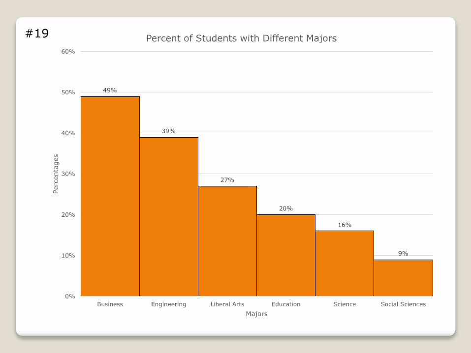
49%
39%
27%
20%
16%
9%
0%
10%
20%
30%
40%
50%
60%
Business Engineering Liberal Arts Education Science Social Sciences
Perc
enta
ges
Majors
Percent of Students with Different Majors#19
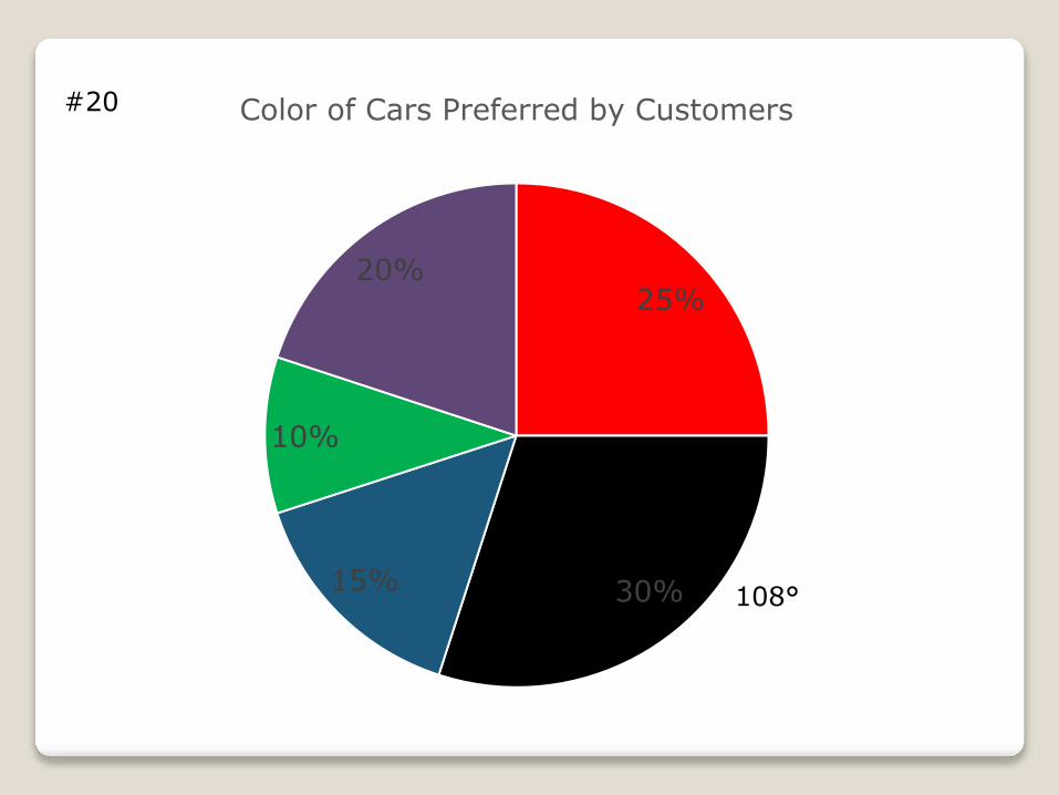
25%
30%15%
10%
20%
Color of Cars Preferred by Customers
108°
#20

Set 2 Set 1
8, 6, 3, 0 1 0, 2
8, 3, 3 2 2, 2, 4, 6, 7
7, 6, 1, 0 3 1, 4, 5, 9
5 4 9
#21
3-3: Measures of VariationObjective: To describe data using measures of variation, such as the
range, variance, and standard deviation.
A testing lab wishes to test two experimental brands of outdoor paint to see how long each will last before fading. The testing lab makes 6 gallons of each paint to test. Since different chemical agents are added to each group and only six cans are involved, these two groups constitute two small populations. The results (in months) are shown. Find the mean of each group.

Brand A Brand B
10 35
60 45
50 30
30 35
40 40
20 25

Mean for brand A:
Mean for brand B:
6
210
N
X
6
210
N
X

Brand A
X X X X X X
10 15 20 25 30 35 40 45 50 55 60
Variation in Paint (in months)
Brand B
X
X X X X X
10 15 20 25 30 35 40 45 50 55 60

Even though the means of the two sets were the same, the spread or variation, was very different.

Three common measures of spread or variability of a set of data:◦ Range
◦ Variance
◦ Standard Deviation

Range: highest value – lowest value◦ “R” is the symbol used for the range

Brand A Brand B
10 35
60 45
50 30
30 35
40 40
20 25
Range for set A: 60 – 10 = 50 months
Range for set B: 45 – 25 = 20 months
Rounding Rule for the Standard Deviation: Same as for the mean. Round to one more decimal place than the original data.
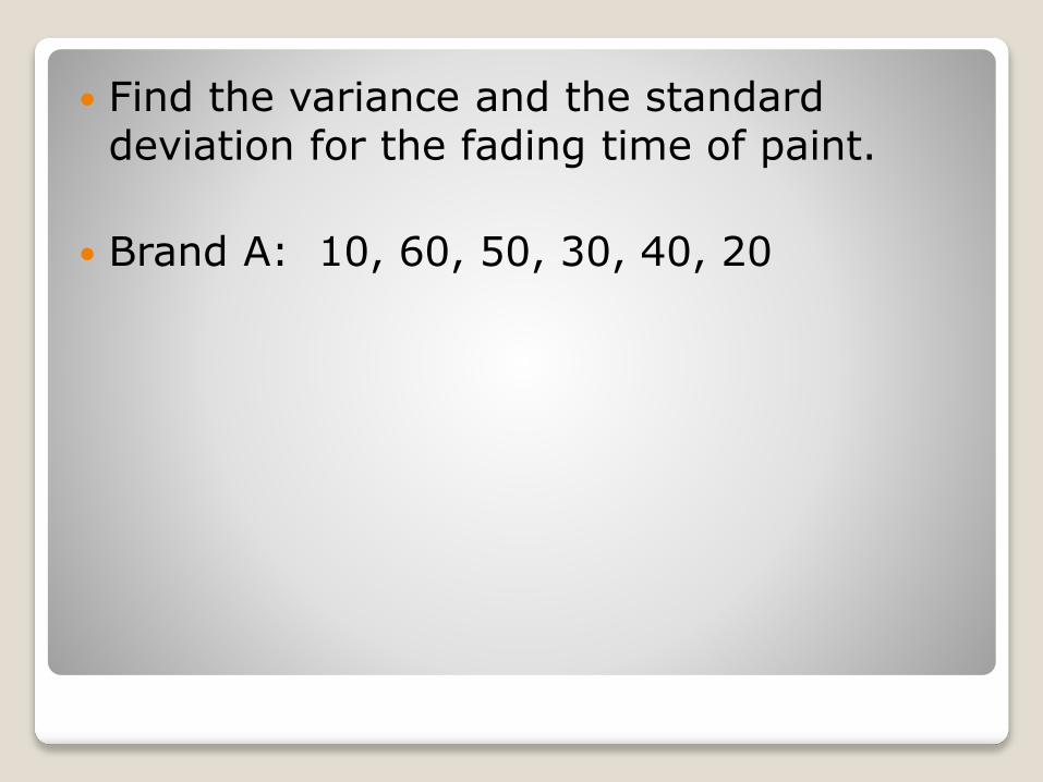
Find the variance and the standard deviation for the fading time of paint.
Brand A: 10, 60, 50, 30, 40, 20

Step 1- Find the mean for the data
356
210
6
204030506010
N
X
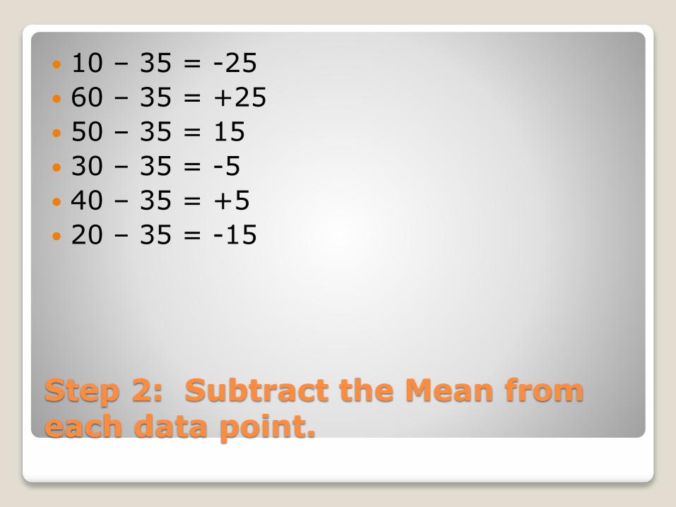
Step 2: Subtract the Mean from each data point.
10 – 35 = -25
60 – 35 = +25
50 – 35 = 15
30 – 35 = -5
40 – 35 = +5
20 – 35 = -15
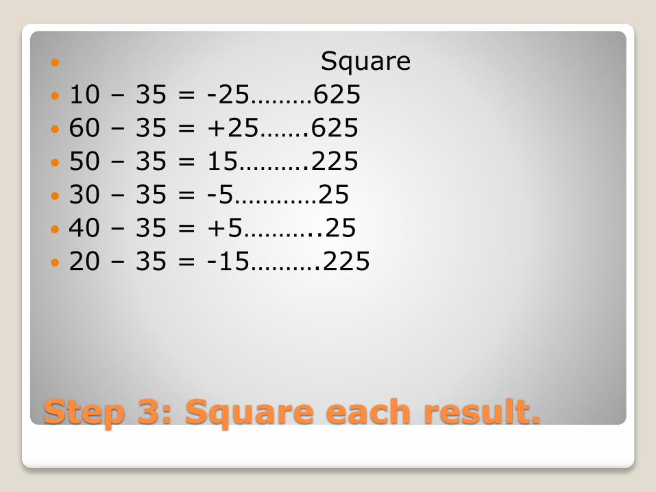
Step 3: Square each result.
Square
10 – 35 = -25………625
60 – 35 = +25…….625
50 – 35 = 15……….225
30 – 35 = -5…………25
40 – 35 = +5………..25
20 – 35 = -15……….225

Step 4: Find the sum of the squares
625 + 625 + 225 + 25 + 25 + 225 = 1750

Step 5: Divide the sum by N to get the variance.
1750 ÷ 6 = 291.7
Variance = 291.7

Step 6: Standard Deviation is the square root of the variance.
1.177.291
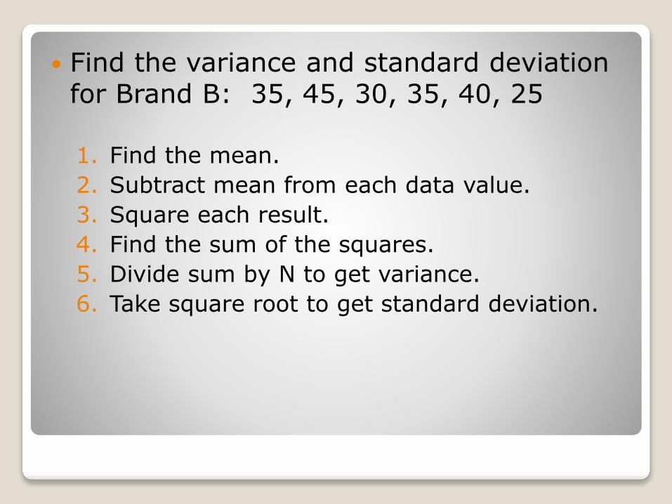
Find the variance and standard deviation for Brand B: 35, 45, 30, 35, 40, 25
1. Find the mean.
2. Subtract mean from each data value.
3. Square each result.
4. Find the sum of the squares.
5. Divide sum by N to get variance.
6. Take square root to get standard deviation.

A B C
X 2. X-μ 3. (X-μ)²
35 35-35=0 0²=0
45 45-35=10 10²=100
30 30-35=-5 (-5) ²=25
35 35-35=0 0²=0
40 40-35=5 5²=25
25 25-35=-10 (-10) ²=100
1. Calculate the mean: 210/6 = 35 months 4. Find the sum of column C: 0+100+25+0+25+100=2505. Divide sum (step 4) by N to get the variance: 250/6=41.76. Take square root of the variance (step 5) to get the
standard deviation: 5.6
6
250

Compare set A to set B
Any conclusions? (see slide 10)
Set A Set B
Variance 291.7 41.7
Standard Deviation 17.1 6.5

Variance: The average of the squares of the distance each value point is from the mean.
Symbol: σ² Population Variance:
Where X: individual valueμ: population meanN: population size
N
X 2
2)(

Standard Deviation: square root of the variance.
Symbol: σ
Population Standard Deviation:
N
X
2
2)(

Sample Variance
1
)( 2
2
n
XXs
Where
X
X
= individual value= sample mean
n = sample size

Sample Standard Deviation
1
)( 2
2
n
XXss
Where
X
X
= individual value= sample mean
n = sample size
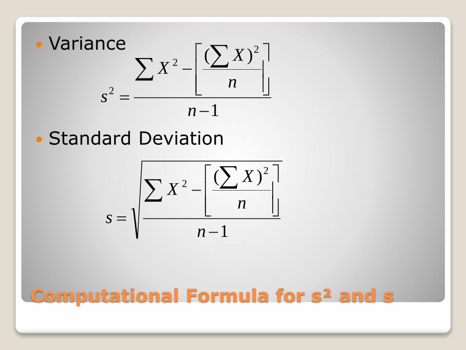
Computational Formula for s² and s
Variance
Standard Deviation
1
)( 2
2
2
n
n
XX
s
1
)( 2
2
n
n
XX
s
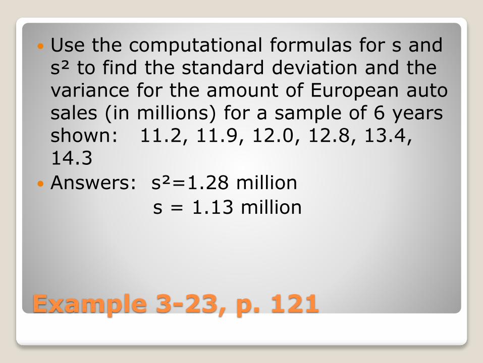
Example 3-23, p. 121
Use the computational formulas for s and s² to find the standard deviation and the variance for the amount of European auto sales (in millions) for a sample of 6 years shown: 11.2, 11.9, 12.0, 12.8, 13.4, 14.3
Answers: s²=1.28 million
s = 1.13 million

Variance and Standard Deviation for Grouped Data
Procedure for finding the variance and standard deviation for grouped data is similar to that for finding the mean for grouped data: use the midpoint.
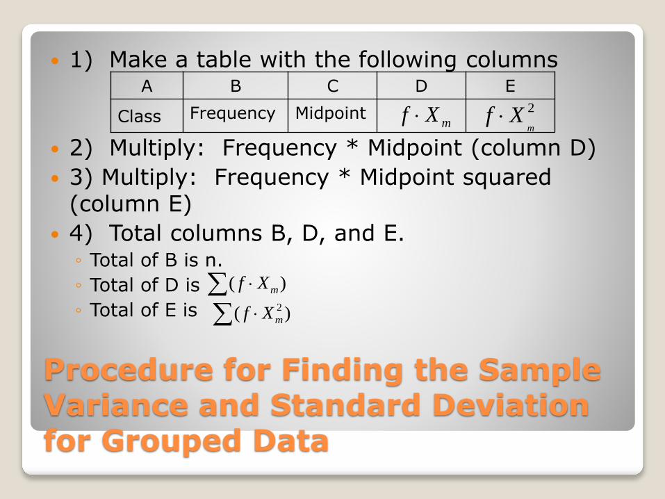
Procedure for Finding the Sample Variance and Standard Deviation for Grouped Data
1) Make a table with the following columns
2) Multiply: Frequency * Midpoint (column D)
3) Multiply: Frequency * Midpoint squared (column E)
4) Total columns B, D, and E. ◦ Total of B is n.
◦ Total of D is
◦ Total of E is
A B C D E
Class Frequency MidpointmXf 2
mXf
)( mXf
)( 2
mXf

Grouped Data-Variance & Standard Deviation cont’d
5) Substitute values from step 4 into
6) Take the square root of the variance (step 5) to find the standard deviation.
1
)()(
2
2
2
n
n
XfXf
s
m
m

Uses of Variance and Standard Deviation
Determine spread of data (large values mean data is fairly spread out)
Determine consistency of a variable. (Nuts & bolts diameters must have small variance & st. dev.)
Used to determine how many data values fall within certain interval. (Chebyshev-75% within 2 st. dev. of mean).
Used in inferential statistics (we’ll see how later).

Coefficient of Variation
Allows comparison of data with different units (number of sales per salesperson vs. commissions made by salesperson).
Coefficient of Variation:◦ Denoted: Cvar
◦ For Samples:
◦ For Populations:
%100X
sCVar
%100
CVar

Example-Coefficient of Variation
Example 3-25
The mean of the number of sales of cars over a 3-month period is 87 and the standard deviation is 5. The mean of the commissions is $5225 and the standard deviation is $773. Compare the variations of the two.
Sales:
Commission:
%7.5%10087
5
X
sCVar
%8.14%1005225
773
CVar
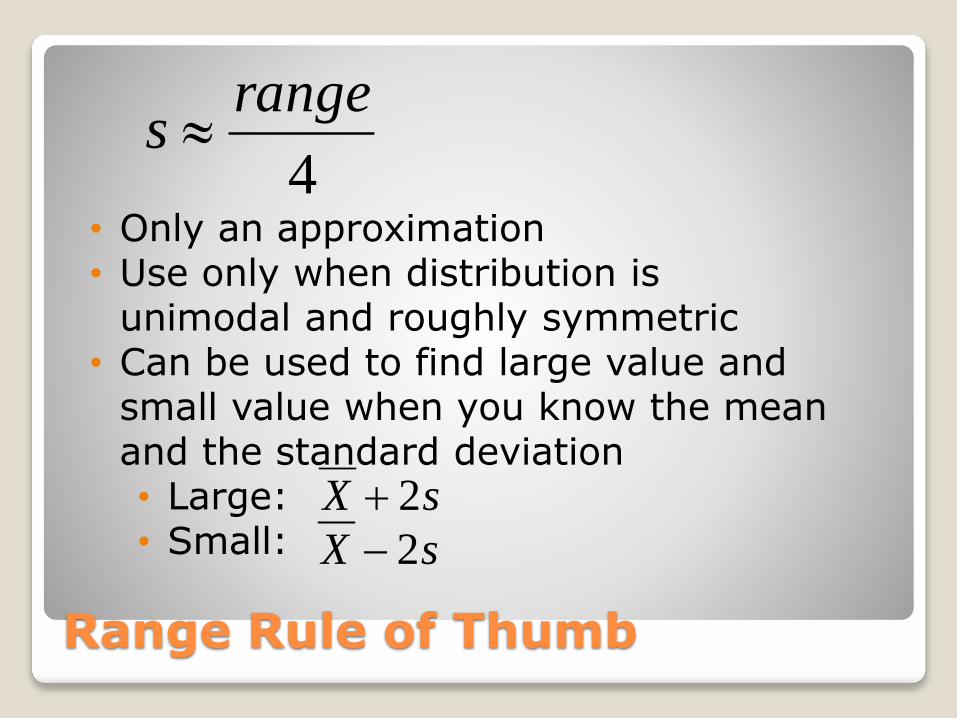
Range Rule of Thumb
4
ranges
• Only an approximation• Use only when distribution is
unimodal and roughly symmetric• Can be used to find large value and
small value when you know the mean and the standard deviation• Large:• Small:
sX 2
sX 2
For many sets of data, almost all values fall within 2 standard deviations of the mean.
Better approximations can be obtained by using Chebyshev’s Theorem.

Chebyshev’s Theorem
Specifies the proportions of the spread in terms of the standard deviation (for any shaped distribution)
Theorem states: The proportion of values from a data set that will fall within k standard deviations of the mean, will be at least
where k is a number greater than 1 (k is not necessarily an integer).
2
11
k
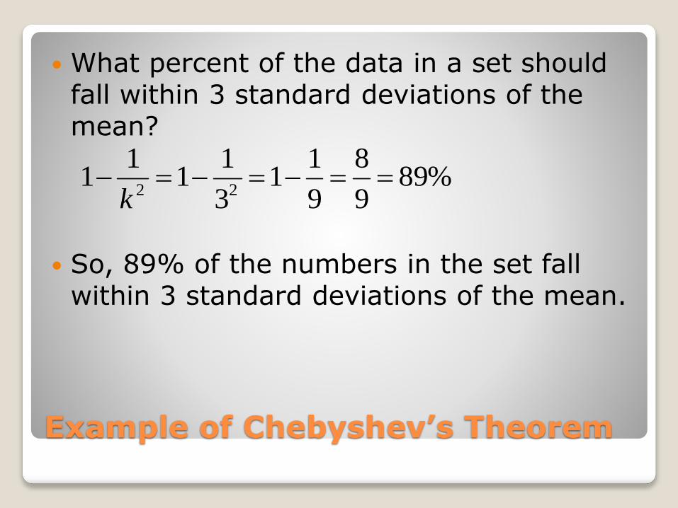
Example of Chebyshev’s Theorem
What percent of the data in a set should fall within 3 standard deviations of the mean?
So, 89% of the numbers in the set fall within 3 standard deviations of the mean.
%899
8
9
11
3
11
11
22
k

Empirical Rule
Applies only to bell-shaped (normal-shaped) distributions.
Rule states:
◦ Approximately 68% of the data values fall within 1 standard deviation of the mean.
◦ Approximately 95% of the data values fall within 2 standard deviations of the mean.
◦ Approximately 99.7% of the data values fall within 3 standard deviations of the mean.
See Figure 3-4, top of p. 128

Homework
p.129-132
#1-5, 7, 11, 13, 19, 31-41 odd
Recommended