Attribution-NonCommercial-NoDerivs 2.0 KOREA
You are free to :
Share — copy and redistribute the material in any medium or format
Under the follwing terms :
Attribution — You must give appropriate credit, provide a link to the license, and
indicate if changes were made. You may do so in any reasonable manner, but
not in any way that suggests the licensor endorses you or your use.
NonCommercial — You may not use the material for commercial purposes.
NoDerivatives — If you remix, transform, or build upon the material, you may
not distribute the modified material.
You do not have to comply with the license for elements of the material in the public domain or where your use
is permitted by an applicable exception or limitation.
This is a human-readable summary of (and not a substitute for) the license.
Disclaimer
공학박사 학위논문
Instance-based Hierarchical Schema
Alignment in Linked Data
링크드 데이터에 대한 인스턴스 기반 온톨로지
매핑
2015 년 8 월
서울대학교 대학원
치의과학과 의료경영과정보학 전공
NANSU ZONG
Abstract
Instance-based Hierarchical Schema
Alignment in Linked Data
Nansu Zong
Medical Management and Informatics
The Graduate School
Seoul National University
Along with the development of Web of documents, there is a natural need for sharing,
exchanging, and merging heterogeneous data to provide more comprehensive
information and answer users with more complex questions. However, the data
published on the Web are raw dumps that sacrifice much of the semantics that can
be used for exchanging and integrating data. Resource Description Framework
(RDF) and Linked Data are designed to expose the semantics of data by
interlinking data represented with well-defined relations. With the profusion of
RDF resources and Linked Data, ontology alignment has gained significance in
providing highly comprehensive knowledge embedded in disparate sources.
Ontology alignment, however, in Linking Open Data (LOD) has traditionally
focused more on the instance-level rather than the schema-level. Linked Data
supports schema-level matching, provided that instance-level matching is already
established. Linked Data is a hotbed for instance-based schema matching, which is
considered a better solution for matching classes with ambiguous or obscure names.
In this dissertation, the author focuses on three issues in instance-based schema
alignment for Linked Data: (1) how to align schemas based on instances, (2) how
to scale the schema alignment, (3) how to generate a hierarchical schema structure.
Targeting the first issue, the author has proposed an instance-based schema
alignment algorithm called IUT. The IUT builds a unified taxonomy for the classes
from two ontologies based on an instance-class matrix and obtains the relations of
two classes by the common instances. The author tested the IUT with DBpedia and
YAGO2, and compared the IUT with two state-of-the-art methods in four alignment
tasks. The experiments show that the IUT outperforms the methods in terms of
efficiency and effectiveness (e.g., costs 968 ms to obtain 0.810 F-score on
intra-subsumption alignment in DBpedia).
Targeting the second issue, the author has proposed a scaled version of the
IUT called IUT(M). The IUT(M) decreases the computations of the IUT from two
aspects based on Locality Sensitive Hashing (LSH): (1) decreasing the similarity
computations for each pair of classes with MinHash functions, and (2) decreasing
the number of similarity computations with banding. The author tested the IUT(M)
with YAGO2-YAGO2 intra-subsumption alignment task to demonstrate that the
running time of IUT can be reduced by 94% with a 5% loss in F-score.
Targeting the third issue, the author has proposed a method to generate a
faceted taxonomy based on object properties on Linked Data. A framework is
proposed to build a sub-taxonomy in each facet with sub-data, extracted with an
object property, with an Instance-based Concept Taxonomy generation algorithm

called ICT. Two experiments demonstrate: (1) The ICT efficiently and effectively
generates a sub-taxonomy with “rdf:type” in DBpedia and YAGO2 (e.g., costs 49
and 11,790 ms to build the concept taxonomies that achieve 0.917 and 0.780 on
Taxonomic F-score). (2) The faceted taxonomies for Diseasome and DrugBank,
efficiently generated based on multiple object properties (e.g., costs 2,032 and
2,525 ms to build the faceted taxonomies based on 6 and 16 properties), can
effectively reduce the search spaces in faceted searches (e.g., obtains 1.65 and 1.03
on Maximum Resolution with 2 facets).
Keywords: Schema Alignment, Instance-based Matching, Linked Data,
Scaling Alignment, Hierarchy Generation
Student Number: 2010-31375
i
Contents
1 Introduction ...................................................................................................... 1
1.1 Background and Motivations ......................................................................... 1
1.1.1 Data Integration and Schema Alignment ................................................ 1
1.1.2 From RDF to Linked Data ...................................................................... 3
1.1.3 Schema Alignment in Linked Data ......................................................... 5
1.2 Instance-based Schema Alignment ................................................................ 9
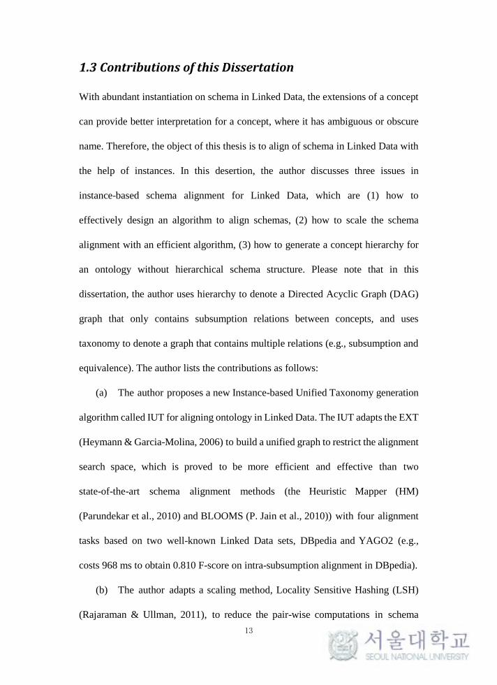
1.3 Contributions of this Dissertation ................................................................ 13
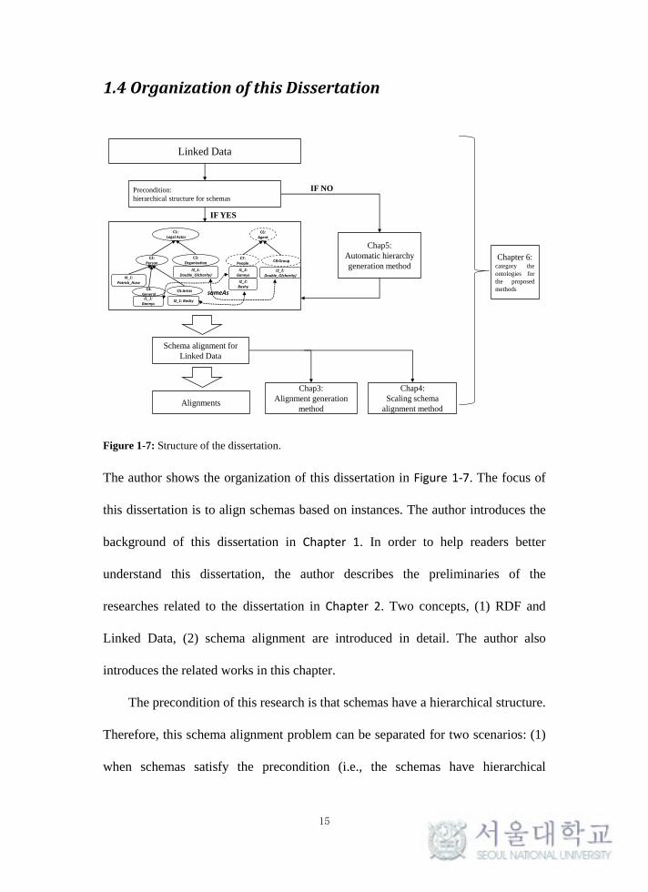
1.4 Organization of this Dissertation .................................................................. 15
2 Preliminaries and Related Works ................................................................... 17
2.1 Preliminaries ................................................................................................ 17
2.1.1 RDF and Linked Data ........................................................................... 17
2.1.2 Ontology and Schema Alignment in Linked Data ................................ 20
2.2 Related Works .............................................................................................. 23
2.2.1 Instance-based Schema Alignment ....................................................... 23
2.2.2 Scaling Pairwise Similarity Computations ............................................ 29
2.2.3 Automatic Taxonomy Generation ......................................................... 32
3 Aligning Schemas with Subsumption and Equivalence Relations ................. 36
3.1 Introduction .................................................................................................. 36
3.2 Problem Definition ....................................................................................... 38
3.3 Methods ........................................................................................................ 41
ii
3.3.1 Workflow of Instance-based Schema Alignment .................................. 41
3.3.2 Instance-class Matrix Generation .......................................................... 42
3.3.3 Subsumption and Equivalence Relations Discovering .......................... 44
3.4 Experiments .................................................................................................. 48
3.4.1 Schema Alignment Algorithms in Comparison .................................... 48
3.4.2 Data and Experiment Design ................................................................. 48
3.5 Results .................................................................................................... 52
3.5.1 Intra-subsumption Relations for YAGO2-YAGO2............................... 54
3.5.2 Intra-subsumption Relations for DBpedia-DBpedia ............................. 58
3.5.3 Inter-Subsumption and Equivalence Relations for YAGO2-DBpedia .. 61
3.5.4 Effects of 𝜒𝑠 and 𝜒𝑒 for the IUT ......................................................... 67
3.6 Discussions ................................................................................................... 71
3.7 Conclusion .................................................................................................... 75
4 Scaling Pair-wise Computations Using the Locality Sensitive Hashing ........ 76
4.1 Introduction .................................................................................................. 76
4.2 Methods ........................................................................................................ 78
4.2.1 MinHash and Signatures ....................................................................... 79
4.2.2 Banding Technique ............................................................................... 83
4.2.3 Scaling the IUT with MinHash and Banding ........................................ 85
4.3 Experiment ................................................................................................... 87
4.4 Discussions ................................................................................................... 92
4.5 Conclusion .................................................................................................... 93
iii
5 Unsupervised Hierarchical Schema Structure Generation in Linked Data .... 94
5.1 Introduction .................................................................................................. 94
5.2 Faceted Taxonomy for Linked Data ............................................................. 98
5.3 Framework ................................................................................................. 101
5.3.1 Facets Extraction ................................................................................. 102
5.3.2 Instance Restriction and Redundancy Removal .................................. 102
5.3.3 Redundant Object Removal................................................................. 103
5.3.4 Instance-object Matrix Generation ...................................................... 103
5.4 Generating Faceted Taxonomy .................................................................. 105
5.4.1 The Problem of Generating a Sub-taxonomy for a Facet .................... 105
5.4.2 Concept Definition and Naming.......................................................... 105
5.4.3 Taxonomy Generation Algorithm ....................................................... 108
5.4.4 Instantiation and Taxonomy Refinement ............................................ 110
5.5 Experiments ................................................................................................ 112
5.5.1 Task 1-Construction of Taxonomy with “rdf:type” ............................ 112
5.5.2 Task 2-Construction of Multiple Faceted Taxonomies ....................... 115
5.6 Results ........................................................................................................ 119
5.6.1 Results of Task 1 ................................................................................. 119
5.6.2 Results of Task 2 ................................................................................. 124
5.7 Discussion .................................................................................................. 131
5.8 Conclusion .................................................................................................. 133
6 Future Works and Conclusion ...................................................................... 134
iv
6.1 Future Works .............................................................................................. 134
6.1.1 Similarity Measures for Instance-based Schema Alignment ............... 134
6.1.2 Ontology Evolution for Instance-based Schema Alignment ............... 135
6.1.3 Combining the IUT with Structure- and Lexical-based Methods ....... 136
6.1.4 Scaling the IUT with Parallel Computations ....................................... 137
6.1.5 Faceted Navigation and Search for Linked Data ................................. 137
6.2 Conclusion .................................................................................................. 139
Bibliography ......................................................................................................... 142
초록 ...................................................................................................................... 152
v
List of Tables
Table 2-1: Comparison of schema alignment methods. ......................................... 27
Table 3-1: Statistic information of the data sets. .................................................... 49
Table 3-2: Results of subsumption alignment in YAGO2-YAGO2. ..................... 55
Table 3-3: Results of subsumption alignment in DBpedia-DBpedia. .................... 59
Table 3-4: Results of subsumption alignment in YAGO2-DBpedia. ..................... 62
Table 3-5: Results of equivalence alignment in YAGO2-DBpedia. ...................... 65
Table 4-1: Efficiency of scaling the IUT for alignment in YAGO2-YAGO2
(𝑣𝑠 = 1,000). .......................................................................................................... 87
Table 4-2: Precision of scaling the IUT for alignment in YAGO2-YAGO2
(𝑣𝑠 = 10,00). .......................................................................................................... 88
Table 4-3: Recall of scaling the IUT for alignment in YAGO2-YAGO2
(𝑣𝑠 = 1,000). .......................................................................................................... 88
Table 4-4: F-score of scaling the IUT for alignment in YAGO2-YAGO2
(𝑣𝑠 = 1,000). .......................................................................................................... 89
Table 5-1. Statistic of the data sets originally and after pre-processed. ............... 113
Table 5-2. Statistic of the two data sets. ............................................................... 115
Table 5-3. Results of conceptualizing disease and drug instances with multiple
object properties. .................................................................................................. 126
Table 6-1. Summarization of the conditions for the proposed methods. .............. 141
vi
List of Figures
Figure 1-1: Data integration methods. ...................................................................... 2
Figure 1-2: Data format evolution of Semantic Web. .............................................. 4
Figure 1-3: Growth of LOD. .................................................................................... 6
Figure 1-4: An example of linked data set. .............................................................. 8
Figure 1-5: Classification of schema matching approaches. .................................... 9
Figure 1-6: Equivalent concept alignment based on instances. .............................. 12
Figure 1-7: Structure of the dissertation. ................................................................ 15
Figure 2-1: An example of RDF/XML and N-Triples formatted RDF documents.
................................................................................................................................ 18
Figure 2-2: De-reference a Web resource. ............................................................. 19
Figure 2-3: Two strategies for scaling pairwise computations. .............................. 30
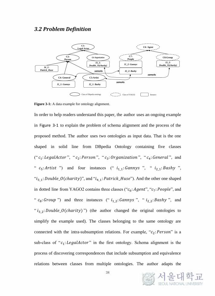
Figure 3-1: A data example for ontology alignment. ............................................. 38
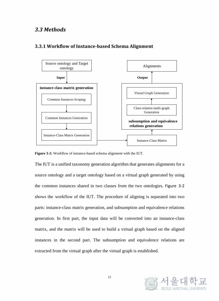
Figure 3-2: Workflow of instance-based schema alignment with the IUT. ........... 41
Figure 3-3: An example of instance-class matrix generation. ................................ 42
Figure 3-4: F-score and running time of the methods. ........................................... 52
Figure 3-5: Running time of the three methods for YAGO2-YAGO2. ................. 54
Figure 3-6: Running time of the three methods of DBpedia-DBpedia. ................. 58
Figure 3-7: Running time of the three methods of YAGO2-DBpedia for
inter-subsumption alignment. ................................................................................. 61
Figure 3-8: Running time of the three methods of YAGO2-DBpedia for
equivalence alignment. ........................................................................................... 64
Figure 3-9: 𝜒𝑠 and 𝜒𝑒 for the IUT. ..................................................................... 69
Figure 4-1: The search spaces of different algorithms in Section 3.4. ................... 76
Figure 4-2: Workflow of scaling the IUT with the LSH. ....................................... 78
vii
Figure 4-3: An example of a matrix based on the instance-class matrix used in
Section 3.3.2 with a permutated order of instances. ............................................... 80
Figure 4-4: An example of computing signatures with the fast MinHashing
algorithm. ............................................................................................................... 82
Figure 4-5: Signatures and buckets with two hash functions. ................................ 83
Figure 4-6: S-curves of 1 − (1 − 𝑠𝑣𝑟)𝑣𝑏 with different combinations of 𝑣𝑟 and
𝑣𝑏 when using 50 hash functions. ......................................................................... 84
Figure 4-7: Efficiency comparison of the IUT and the IUT(M) that with 𝑣𝑟 = 2
and 𝑣𝑠 = 1,000. ..................................................................................................... 91
Figure 5-1. A faceted taxonomy for a sample of Linked Data. .............................. 98
Figure 5-2. The framework of faceted taxonomy construction. ........................... 101
Figure 5-3. An ongoing example of building a sub-taxonomy with an object
property “Diseasome:possibleDrug” partially extracted from Diseasome. ......... 102
Figure 5-4. TF-score and running time of the methods.. ...................................... 120
Figure 5-5. TP-scores of ICT for DBpedia and YAGO2 with different 𝜑. ......... 123
Figure 5-6. Running time of building a sub-taxonomy with a single property. ... 124
Figure 5-7. Average running time of building faceted taxonomies with different
facets (properties). ................................................................................................ 127
Figure 5-8. Maximum Resolution scores with different facets (properties). ....... 129
Figure 5-9. Number of top 500 important concetps in each sub-taxonomy in a
faceted taxonomy. ................................................................................................ 130
1
1 Introduction
1.1 Background and Motivations
1.1.1 Data Integration and Schema Alignment
Information, along with our human civilization development, is the basic human
need. Data that supplies users with abundant information is stored scattered in
different repositories. Along with the increasing of data, there is a natural need of
sharing, exchanging, and merging heterogeneous data to provide more
comprehensive information and answer users with more complex questions. For
example, an integration of data on diseases and genes can help users to better
understand the mechanism of diseases. The data integration minimizes the
inconsistency of data formats and specifications, and decreases redundant data in
different sources.
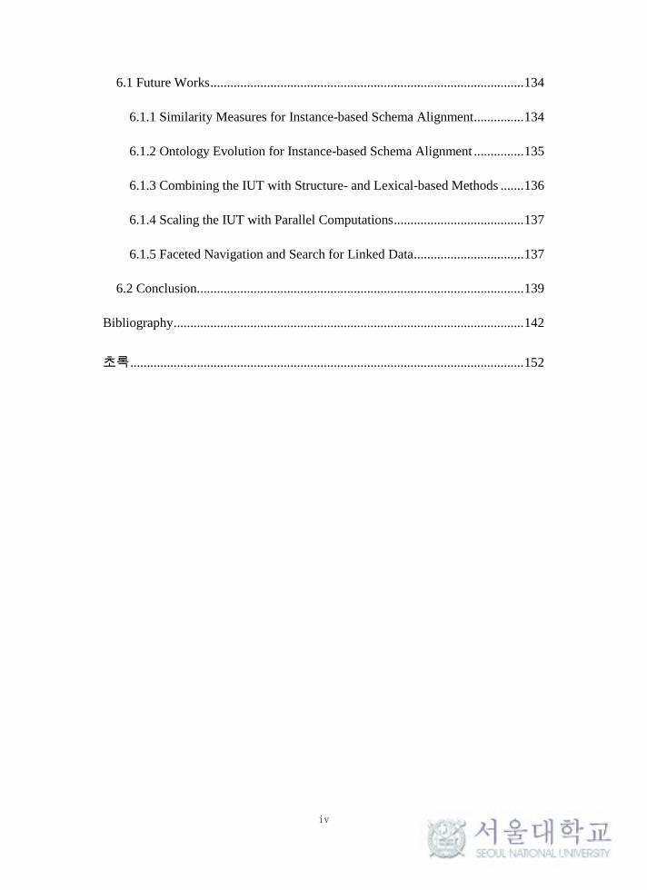
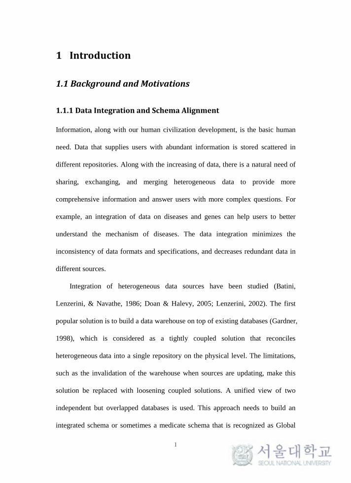
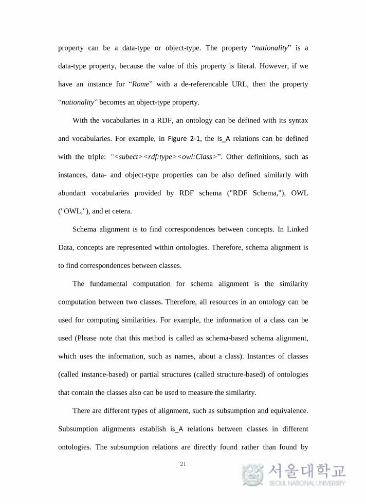
Integration of heterogeneous data sources have been studied (Batini,
Lenzerini, & Navathe, 1986; Doan & Halevy, 2005; Lenzerini, 2002). The first
popular solution is to build a data warehouse on top of existing databases (Gardner,
1998), which is considered as a tightly coupled solution that reconciles
heterogeneous data into a single repository on the physical level. The limitations,
such as the invalidation of the warehouse when sources are updating, make this
solution be replaced with loosening coupled solutions. A unified view of two
independent but overlapped databases is used. This approach needs to build an
integrated schema or sometimes a medicate schema that is recognized as Global
2
Schema Pattern. The object of this method is to unify data, which heavily relies on
the stability of data sources. When the structures of some data sources change, the
whole unified global schema needs to be redefined (L. Xu, Xu, Tjoa, & Chaudhry,
2007). Another solution is using a transformation pattern (Czarnecki & Helsen,
2006) to exchanging data instead of unifying data. The two methods both require
the establishment of correspondences between schemas of different data sources.
Therefore, schema alignment or schema matching is one of the fundamental tasks
in realizing data integration.
Figure 1-1: Data integration methods.
Database A Database B
Schema A Schema B
Database A Database B
Data Warehouse
Database A Database B
Schema A Schema B
Integrated
Schema
Alignments (A-B)
Level of data coupled
tightly
loosening
Database c
Schema C
Database C
Database C
Schema C
Alignments (B-C)
Alignments (A-C)
3
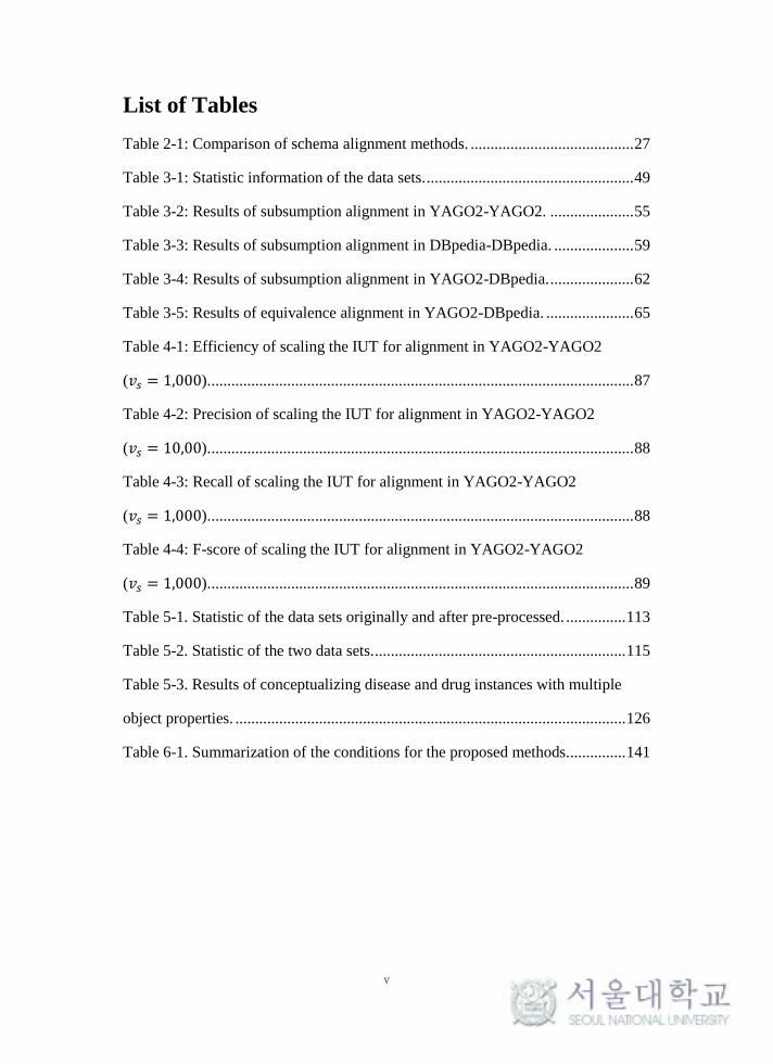
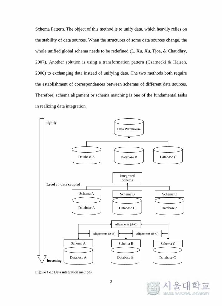
1.1.2 From RDF to Linked Data
Along with the development of the Internet, more and more data are published on
Web that lowers the expense of publishing and accessing information. The data
published on the Web are raw dumps formatted as CSV, XML, or HTML tables,
which sacrifices much of the semantics (Bizer, Heath, & Berners-Lee, 2009). The
semantics behind the data defines the context or meaning of the data, and helps
exchanging data in business or other areas. In traditional hypertext Web, semantics
of a document is implicit. For example, “apple” can denote an information
technology company or a kind of fruit in different documents. Exchanging data
between documents sometimes require more man-powers to understand the
semantics behind documents.
Therefore, expressing information under a description framework is needed.
Resource Description Framework (RDF) supports data merging and schema
evolution by explicating the semantics behind data ("Resource Description
Framework (RDF),"). RDF is designed to expose the semantics of data for
machines to understand. The concepts used in the schema of one data set are
defined and connected with other related concepts in the same data under an RDF
document. For example, the same concept “apple” used in two different data
sources, can be distinguished by the definitions of the concept “apple” with two
RDF documents. Even though, the semantics can be exposed with RDF, the data
interlinking between different sources still not be accomplished. In order to create
a global information space of both linked document and data, data (i.e., entities
that are classes or instances) contained in RDF documents starts to link, which is
4
called Linked Data. Linked Data refers to the data set that is published on the Web
with a machine-readable format (e.g., RDF) and links to external RDF data sets,
and further can be linked as an external data set for other RDF data. Figure 1-2
shows the evolution of data format in Semantic Web.
Figure 1-2: Data format evolution of Semantic Web.
Database A Database B
Schema A Schema B
RDF
document
RDF
document
semanticssemantics
Linked Data Linked Data
5
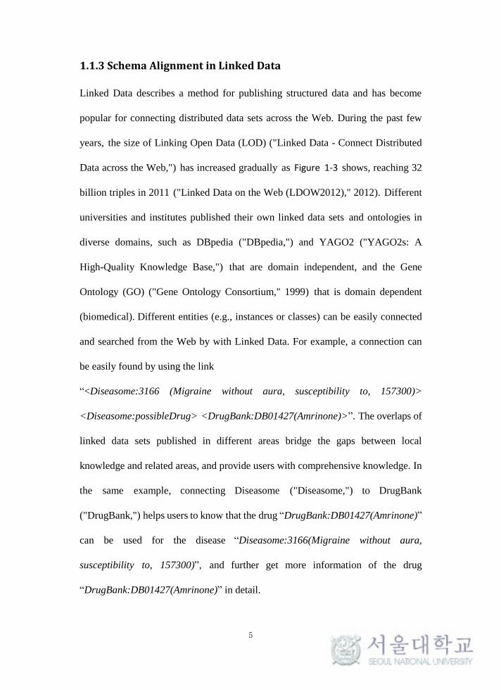
1.1.3 Schema Alignment in Linked Data
Linked Data describes a method for publishing structured data and has become
popular for connecting distributed data sets across the Web. During the past few
years, the size of Linking Open Data (LOD) ("Linked Data - Connect Distributed
Data across the Web,") has increased gradually as Figure 1-3 shows, reaching 32
billion triples in 2011 ("Linked Data on the Web (LDOW2012)," 2012). Different
universities and institutes published their own linked data sets and ontologies in
diverse domains, such as DBpedia ("DBpedia,") and YAGO2 ("YAGO2s: A
High-Quality Knowledge Base,") that are domain independent, and the Gene
Ontology (GO) ("Gene Ontology Consortium," 1999) that is domain dependent
(biomedical). Different entities (e.g., instances or classes) can be easily connected
and searched from the Web by with Linked Data. For example, a connection can
be easily found by using the link
“<Diseasome:3166 (Migraine without aura, susceptibility to, 157300)>
<Diseasome:possibleDrug> <DrugBank:DB01427(Amrinone)>”. The overlaps of
linked data sets published in different areas bridge the gaps between local
knowledge and related areas, and provide users with comprehensive knowledge. In
the same example, connecting Diseasome ("Diseasome,") to DrugBank
("DrugBank,") helps users to know that the drug “DrugBank:DB01427(Amrinone)”
can be used for the disease “Diseasome:3166(Migraine without aura,
susceptibility to, 157300)”, and further get more information of the drug
“DrugBank:DB01427(Amrinone)” in detail.
6
Figure 1-3: Growth of LOD. (this figure is originated from the paper (Heath & Bizer, 2011).)
7
Driving by the benefits behind the interoperability and information integration,
ontology alignment has been studied for years (S. Wang, Englebienne, & Schlobach,
2008), but it still lacks the study in Linked Data. The terms “alignment” and
“matching” denote a process in which to find correspondences between concepts,
whereas mapping can be defined as the products of alignment or matching
(Bellahsene, Bonifati, & Rahm, 2011; Miller, Haas, & Hernández, 2000).
Conventionally, “alignment” is frequently used for Ontology and “matching” is
primarily used in Database area (Bellahsene et al., 2011). In order to avoid the
ambiguities that may affect the understanding of readers, the author uses
“alignment” primarily to indicate the process of finding correspondences.
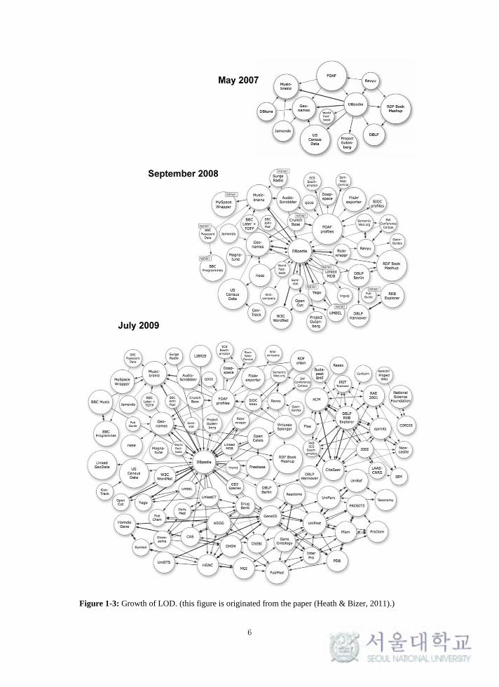
The data in a linked data set normally are constituted of two parts: assertions
and terminologies. The assertions in a link data set normally contain the
information about instances. For example, as shown in Figure 1-4, an entity
“Dbpedia:Gannys” is contained by four triples: (1) has a name “Gannys”, (2) is a
type of “DBpediaOntology:General”, (3) is same as “FreeBase:m.04n2vn1”, and
(4) is the commander of the entity “Dbpedia:Battle_of_Antioch(218)”. The
terminologies contain the information about classes. For example in the same
figure, “DBpediaOntology:General” is a sub-class of “DBpediaOntology:Person”.
Therefore, ontology alignment in Linked Data includes the alignment in
A-Box (Assertion Box) and T-box (Terminology Box). The mappings for A-Box
known as instance-level mapping (i.e., aligning instances from different ontologies)
have received most attention in research, whereas T-Box mappings known as
schema-level mapping are little studied (i.e., aligning schemas from different
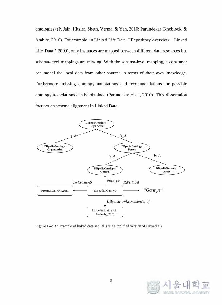
8
ontologies) (P. Jain, Hitzler, Sheth, Verma, & Yeh, 2010; Parundekar, Knoblock, &
Ambite, 2010). For example, in Linked Life Data ("Repository overview - Linked
Life Data," 2009), only instances are mapped between different data resources but
schema-level mappings are missing. With the schema-level mapping, a consumer
can model the local data from other sources in terms of their own knowledge.
Furthermore, missing ontology annotations and recommendations for possible
ontology associations can be obtained (Parundekar et al., 2010). This dissertation
focuses on schema alignment in Linked Data.
Figure 1-4: An example of linked data set. (this is a simplified version of DBpedia.)
DBpediaOntology :
Legal Actor
DBpediaOntology:
Person
DBpediaOntology:
Artist
DBpediaOntology:
General
DBpedia:Gannys
DBpediaOntology:
Organization
FreeBase:m.04n2vn1
DBpedia:Battle_of_
Antioch_(218)
Is_A Is_A
Is_A Is_A
Owl:sameASRdf:type
DBpeida-owl:commander of
Rdfs:label
“Gannys”
9
1.2 Instance-based Schema Alignment
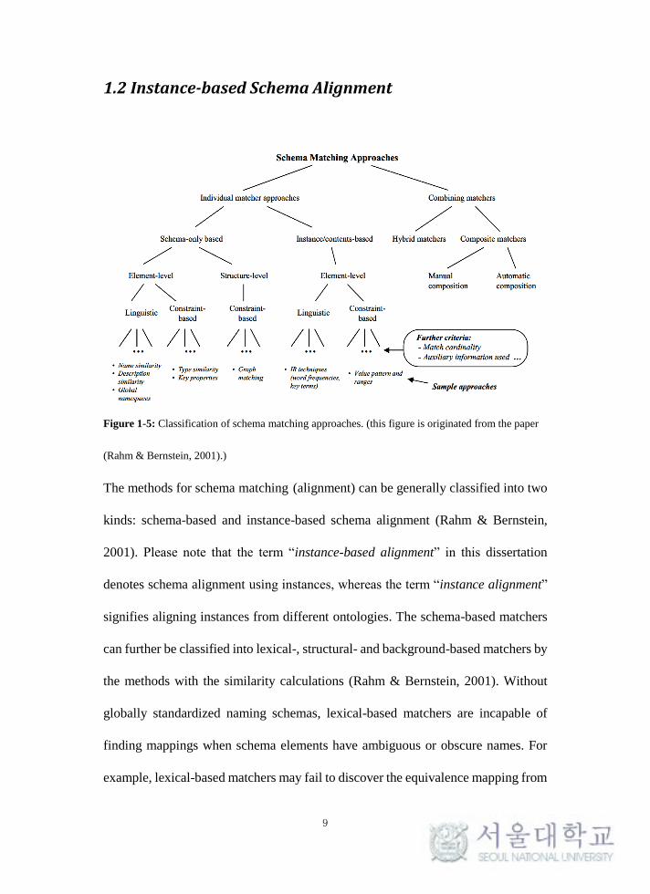
Figure 1-5: Classification of schema matching approaches. (this figure is originated from the paper
(Rahm & Bernstein, 2001).)
The methods for schema matching (alignment) can be generally classified into two
kinds: schema-based and instance-based schema alignment (Rahm & Bernstein,
2001). Please note that the term “instance-based alignment” in this dissertation
denotes schema alignment using instances, whereas the term “instance alignment”
signifies aligning instances from different ontologies. The schema-based matchers
can further be classified into lexical-, structural- and background-based matchers by
the methods with the similarity calculations (Rahm & Bernstein, 2001). Without
globally standardized naming schemas, lexical-based matchers are incapable of
finding mappings when schema elements have ambiguous or obscure names. For
example, lexical-based matchers may fail to discover the equivalence mapping from
10
“DBpediaOntology:Nerve” to “YAGO:FiberBundle”. The structural-based and
background-based methods fail to find mappings when two ontologies have
different granularity in the schema (Kirsten, Thor, & Rahm, 2007). For example,
BLOOMS (P. Jain et al., 2010), a lexical- and structural-based matcher for Linked
Data, fails to find the subsumption relations between DBpedia ontology and
YAGO2 used in Section 3.4. Even though BLOOMS outperformed traditional
schema alignment methods, it is still not sufficient enough in terms of running time
(efficiency) and F-score (effectiveness).
A class (concept) represents a whole group of individuals sharing common
attributes. In ontology, a class is defined by intension or extension ("Class
(philosophy),"). The intension of a class is a set of properties (attributes) shared by
instances to which they apply, whereas the extension is a collection of instances
(individuals) to which they apply.
The problem of identity is a long-standing debate in philosophy, and in linked
data, it is no exception. In Leibnitz’s Law ("The Identity of Indiscernibles," 2010),
two objects are identical, if they have the same description on the intension, which is
adapted to define class equality as well in OWL 2 (Carroll, Herman, &
Patel-Schneider, 2012). Therefore, the alignment of two classes based on the
intensional description (properties) is frequently used for the upper ontologies
where the classes are mostly defined intensionally, such as ontologies in OBO
Foundry. For those ontologies constructed by the software developers and engineers
without training in ontology modeling in Linked Data, the extensional description
11
can stand to match classes, as the identifying characteristics for the identity
conditions (Guarino & Welty, 2002).
It is difficult to keep the consistency of using identity with its logical definition
in the wild, since there are diverse varieties of perceived identity, such as “identical
but referential Opaque”, “identical as claims”, “matching”, and “similar” (Halpin,
Hayes, McCusker, McGuinness, & Thompson, 2010). Without considering the first
two issues (i.e., “identical but referential Opaque” and “identical as claims”) in the
ideal knowledge representation, the “matching” and “similar” are mostly
considered to model identity. In OWL 2, two classes are defined as
“Owl:equivalentClass” if they have the same extensional definition (i.e.,
“matching”) (Carroll et al., 2012). For example, in Figure 1-6 (a), “class 1” and
“class 1’” are considered same when the two classes have the same four instances.
More practical in SKOS, the classes are defined as “Skos:exactMatch” if they have a
high degree of confidence (e.g., similarity) to support themselves to be used
interchangeably, or as “Skos:closeMatch” if they reach a certain level of similarity
("SKOS Simple Knowledge Organization System Reference," 2009).
Similar with the definition used in SKOS for identity in non-ideal knowledge
representation, the author considers that two concepts are equivalent if they reach a
certain level of similarity (i.e., 𝜒𝑒 used in the proposed method) in this dissertation.
Similarly, instead of adapting the strict definition of the subsumption in ideal
knowledge representation, the author considers two concepts have a subsumption
relation if they reach a certain level of containment (i.e., χs used in the proposed
method).
12
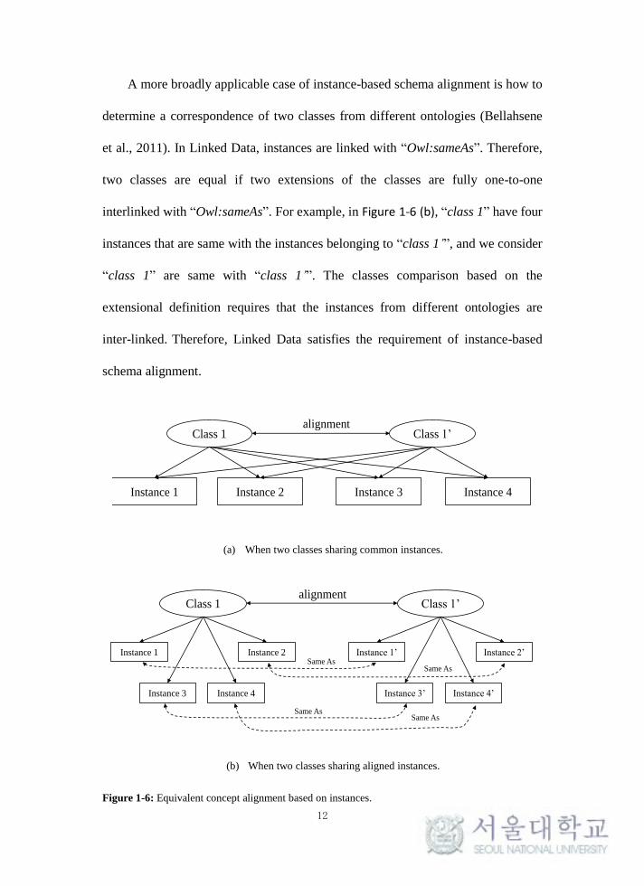
A more broadly applicable case of instance-based schema alignment is how to
determine a correspondence of two classes from different ontologies (Bellahsene
et al., 2011). In Linked Data, instances are linked with “Owl:sameAs”. Therefore,
two classes are equal if two extensions of the classes are fully one-to-one
interlinked with “Owl:sameAs”. For example, in Figure 1-6 (b), “class 1” have four
instances that are same with the instances belonging to “class 1’”, and we consider
“class 1” are same with “class 1’”. The classes comparison based on the
extensional definition requires that the instances from different ontologies are
inter-linked. Therefore, Linked Data satisfies the requirement of instance-based
schema alignment.
(a) When two classes sharing common instances.
(b) When two classes sharing aligned instances.
Figure 1-6: Equivalent concept alignment based on instances.
Class 1 Class 1’
Instance 1 Instance 2 Instance 3 Instance 4
alignment
Instance 1 Instance 2
Instance 3 Instance 4
Class 1
Instance 1’ Instance 2’
Instance 3’ Instance 4’
Class 1’alignment
Same AsSame As
Same AsSame As
13
1.3 Contributions of this Dissertation
With abundant instantiation on schema in Linked Data, the extensions of a concept
can provide better interpretation for a concept, where it has ambiguous or obscure
name. Therefore, the object of this thesis is to align of schema in Linked Data with
the help of instances. In this desertion, the author discusses three issues in
instance-based schema alignment for Linked Data, which are (1) how to
effectively design an algorithm to align schemas, (2) how to scale the schema
alignment with an efficient algorithm, (3) how to generate a concept hierarchy for
an ontology without hierarchical schema structure. Please note that in this
dissertation, the author uses hierarchy to denote a Directed Acyclic Graph (DAG)
graph that only contains subsumption relations between concepts, and uses
taxonomy to denote a graph that contains multiple relations (e.g., subsumption and
equivalence). The author lists the contributions as follows:
(a) The author proposes a new Instance-based Unified Taxonomy generation
algorithm called IUT for aligning ontology in Linked Data. The IUT adapts the EXT
(Heymann & Garcia-Molina, 2006) to build a unified graph to restrict the alignment
search space, which is proved to be more efficient and effective than two
state-of-the-art schema alignment methods (the Heuristic Mapper (HM)
(Parundekar et al., 2010) and BLOOMS (P. Jain et al., 2010)) with four alignment
tasks based on two well-known Linked Data sets, DBpedia and YAGO2 (e.g.,
costs 968 ms to obtain 0.810 F-score on intra-subsumption alignment in DBpedia).
(b) The author adapts a scaling method, Locality Sensitive Hashing (LSH)
(Rajaraman & Ullman, 2011), to reduce the pair-wise computations in schema
14
alignment and call this method IUT(M). The author tests the IUT(M) with YAGO2
(YAGO2-YAGO2) in intra-subsumption task, and demonstrates that the IUT(M)
can effectively reduce the 94% of the original running time with a loss of 5%
F-score.
(c) The author proposes a robust method for generating a faceted taxonomy
based on object properties of instances in Linked Data. The author has developed a
framework that dynamically extracts data with a single object property and
generates a sub-taxonomy in each facet based on an Instance-based Concept
Taxonomy generation algorithm called ICT. Two experiments demonstrate: (1)
The ICT efficiently and effectively generates a sub-taxonomy with “rdf:type” in
DBpedia and YAGO2 (e.g., costs 49 and 11,790 ms to build the concept
taxonomies that achieve 0.917 and 0.780 on Taxonomic F-score). (2) The faceted
taxonomies with Diseasome ("Diseasome,") and DrugBank ("DrugBank,"),
efficiently generated based on multiple object properties (e.g., costs 2,032 and
2,525 ms to build the faceted taxonomies based on 6 and 16 properties), can
effectively reduce the search spaces in faceted searches (e.g., obtains 1.65 and 1.03
on Maximum Resolution with 2 facets).
15
1.4 Organization of this Dissertation
Figure 1-7: Structure of the dissertation.
The author shows the organization of this dissertation in Figure 1-7. The focus of
this dissertation is to align schemas based on instances. The author introduces the
background of this dissertation in Chapter 1. In order to help readers better
understand this dissertation, the author describes the preliminaries of the
researches related to the dissertation in Chapter 2. Two concepts, (1) RDF and
Linked Data, (2) schema alignment are introduced in detail. The author also
introduces the related works in this chapter.
The precondition of this research is that schemas have a hierarchical structure.
Therefore, this schema alignment problem can be separated for two scenarios: (1)
when schemas satisfy the precondition (i.e., the schemas have hierarchical
C1:Legal Actor
C2:Person
C5:ArtistC4:General
I2_1: BashyI1_1:
Gannys
C3:Organization
I4_1:Patrick_Huse
I3_1:Double_O(charity)
C6:Agent
C7:People
I1_2: Gannys
C8:Group
I3_2:Double_O(charity)
sameAs
I2_2: Bashy
Schema alignment for
Linked Data
Chap3:
Alignment generation
method
Chap4:
Scaling schema
alignment method
Linked Data
Precondition:
hierarchical structure for schemas
Chap5:
Automatic hierarchy
generation method
IF YES
Alignments
IF NO
Chapter 6:category the
ontologies for
the proposed
methods
16
structures) in Chapters 3 and 4, and (2) schemas do not satisfy the precondition in
Chapter 5.
For the schemas having a hierarchical structure, the author details the
methodology of instance-based schema alignment in Chapter 3. And in Chapter 4,
the author presents the scaling algorithm based on the LSH.
For those do not have a hierarchical structure, the author proposes a method
of generating a faceted taxonomy automatically in Chapter 5.
Finally, the author concludes the works of this dissertation, and lists several
future works as the research extensions for this dissertation.
17
2 Preliminaries and Related Works
2.1 Preliminaries
2.1.1 RDF and Linked Data
The RDF is a metadata data model for conceptual description or information
expression, which is proposed and promoted by World Wide Web Consortium
(W3C) ("Resource Description Framework (RDF) Model and Syntax
Specification," 1999). Similar with the classic modeling approaches, such as
Entity-Relation (ER) diagrams, the RDF data models resources with statements. A
resource in the RDF denotes a thing that is identified with a de-referencable URL.
A resource can be anything on the Web. For example, a person named “Michael
Jackson” identified with “http://dbpedia.org/page/Michael_Jackson
(Dbpedia:Michael_Jackson)” is a resource. Sometimes, we also call a resource as
an entity. A statement that consists of subject-predicate-object is called triple in
the RDF. A subject in a triple is a resource (entity). An object can be an entity or a
literal text. A predicate, also be called as attribute or property, demonstrates a
relation between a subject and an object. The property can be two types:
object-type and data-type. In a triple, if the object is an entity, the property is the
object-type property. For example, the triple
“<Dbpedia:Michael_Jackson><Rdfs:label> ’Michael Jackson’ ” contains the
data-type property “Rdfs:label”. The triple
“<Dbpedia:Michael_Jackson><foaf:homepage><http://www.michaeljackson.co
m>” contains an object-type property “foaf:homepage”. Since all resources are
18
described with properties, the vocabularies are defined and can be reused by other
RDF documents. For example, the “rdfs:Class”, denoting that a subject is a class,
is defined in “http://www.w3.org/2000/01/rdf-schema#”. The vocabularies defined
by the RDF specification can be found in ("Resource Description Framework
(RDF) Model and Syntax Specification," 1999).
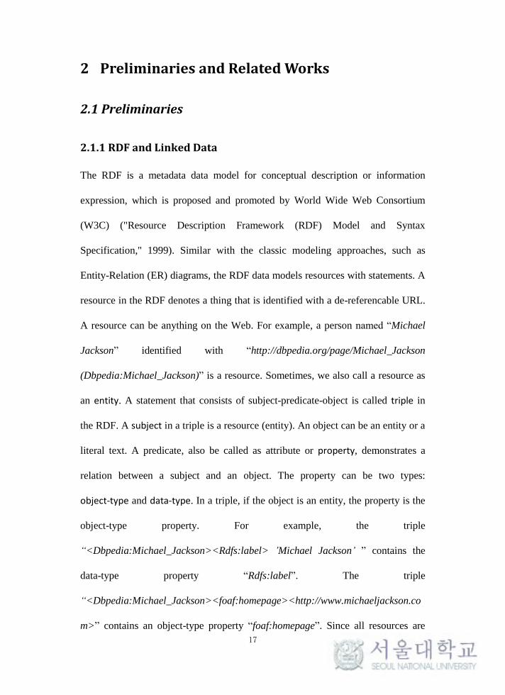
Figure 2-1: An example of RDF/XML and N-Triples formatted RDF documents.
A RDF document can be presented with different formats, such as RDF/XML
and N-Triples. RDF/XML is the first W3C serialization format historically, and it
is gradually replaced with other formats that are more human-readable and less
restrictions on the syntax of XML names ("Resource Description Framework
DbpediaOntology:
Person
DbpediaOntology:
General
Dbpedia:GannysDbpedia:Battle_of_
Antioch_(218)
Is_A
Rdf:typeDbpeida-owl:commander of
Rdfs:label
“Gannys”
<?xml version="1.0"?>
<rdf:RDF xmlns:rdfs="http://www.w3.org/2000/01/rdf-schema#"
xmlns:owl="http://www.w3.org/2002/07/owl#"
xmlns:xsd="http://www.w3.org/2001/XMLSchema#"
xmlns:rdf="http://www.w3.org/1999/02/22-rdf-syntax-ns#">
<owl:Class rdf:about="General">
<rdfs:subClassOf rdf:resource="Person"/>
</owl:Class>
<owl:ObjectProperty rdf:about="commander_of"/>
<owl:NamedIndividual rdf:about="Battle_of_Antioch_(218)"/>
<owl:NamedIndividual rdf:about="Gannys">
<rdf:type rdf:resource="General"/>
<commander_of rdf:resource="Battle_of_Antioch_(218)"/>
<rdf:label rdf:about=“Gannys”>
</owl:NamedIndividual>
</rdf:RDF>
<Person><rdf:type><owl:Class>
<General><rdf:type><owl:Class>
<General><subClassOf><Person>
<Gannys><rdf:type><owl:NamedIndividual>
<Gannys><rdf:type><General>
<Battle_of_Antioch_(218)><rdf:type><owl:NamedIndividual>
<commander_of><rdf:type><owl:ObjectProperty>
<Gannys><commander_of><Battle_of_Antioch_(218)>
<Gannys><rdf:label >"Gannys"
Statement 1
Statement 2
Statement 3
Statement 4
RDF/XML N-Triples
Statement 1
Statement 2
Statement 3
Statement 4
Statement 1
Statement 2
Statement 4
Statement 3
19
(Wiki),"). The author shows an example of RDF/XML and N-Triples formatted
RDF documents of an RDF graph in Figure 2-1.
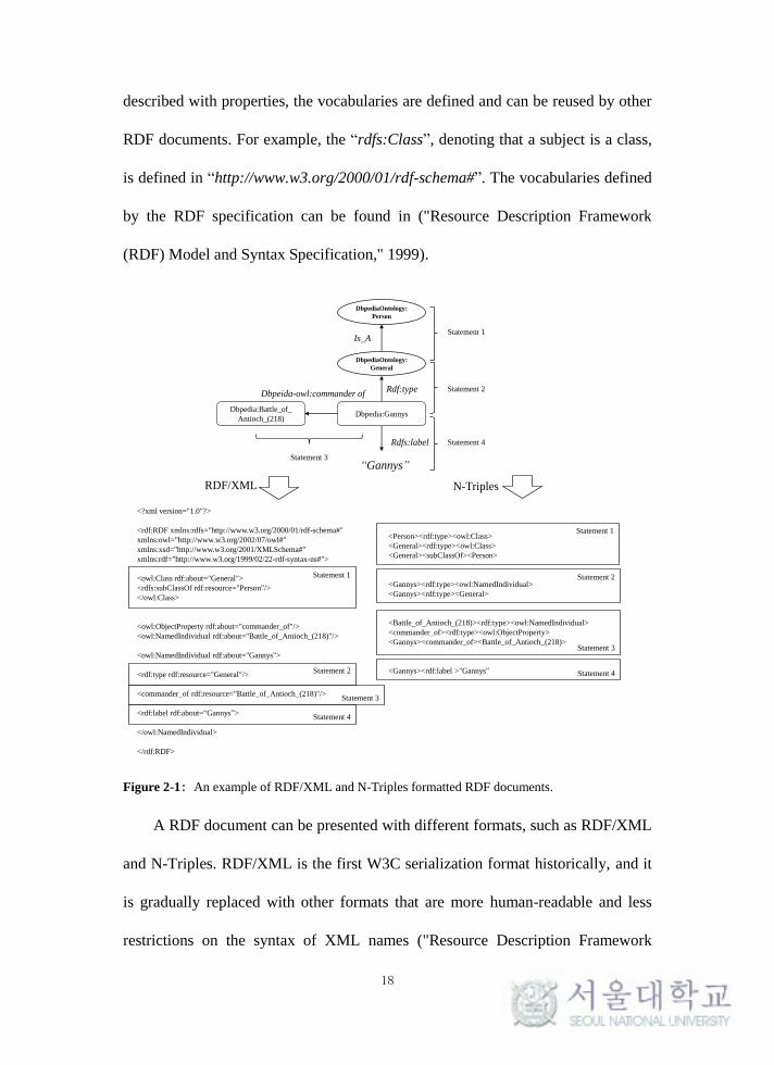
Linked Data uses RDF links to connect a subject with a de-reference URL in
a local set to an object with a URL reference in an external data set. When an
object is de-referenced over the HTTP protocol, a server of this URL will return an
RDF document about the object to a client, which helps users to get more related
information, object in this case, about a subject. The author shows the process of
de-reference in Figure 2-2.
(a) De-reference a vocabulary URL
(b) De-reference a class or property URL
Figure 2-2: De-reference a Web resource. (this figure is originated from ("Best Practice Recipes for
Publishing RDF Vocabularies,").)
20
2.1.2 Ontology and Schema Alignment in Linked Data
As the author mentioned in Section 1.2, Ontology in computer science and
information science is a way of presenting knowledge. Components, such as
classes, instances (i.e., individuals), properties (i.e., attributes or predicates) are
used to present the semantics in an ontology. Please note that, the author only
introduces the components of an ontology that are most frequently used for
schema alignment, other components, such as restrictions and axioms, are not
covered by this section.
Classes in ontology are hierarchical organized, which means that if a class
“general” is a sub concept of a class “people”, the two classes are connected with
an is_A relation. Sub-classes inherit properties from the super class. For example,
if the class “people” has a property “nationality”, the class “general” also has the
property “nationality”. Some ontologies allow multiple inheritance, which means a
class can have multiple super classes. For example, the class “general” can be
sub-class of both the class “people” and a class “job”.
Instances (individual) are used to detail a class. For example, “Gannys” is an
instance of “general”. Instantiation, populating a class with instances, is supported
by inheritance, which means that instances belonging to a sub-class also belong to
its super class. For example, “Gannys” is an instance of the class the class
“general” and its super class “people”.
Properties are used to describe a class, and an instance has specific values of a
property. For example, for the property “nationality” of a class “people”, the
instance of this class “Gannys” can has a value “Rome” for “nationality”. A
21
property can be a data-type or object-type. The property “nationality” is a
data-type property, because the value of this property is literal. However, if we
have an instance for “Rome” with a de-referencable URL, then the property
“nationality” becomes an object-type property.
With the vocabularies in a RDF, an ontology can be defined with its syntax
and vocabularies. For example, in Figure 2-1, the Is_A relations can be defined
with the triple: “<subect><rdf:type><owl:Class>”. Other definitions, such as
instances, data- and object-type properties can be also defined similarly with
abundant vocabularies provided by RDF schema ("RDF Schema,"), OWL
("OWL,"), and et cetera.
Schema alignment is to find correspondences between concepts. In Linked
Data, concepts are represented within ontologies. Therefore, schema alignment is
to find correspondences between classes.
The fundamental computation for schema alignment is the similarity
computation between two classes. Therefore, all resources in an ontology can be
used for computing similarities. For example, the information of a class can be
used (Please note that this method is called as schema-based schema alignment,
which uses the information, such as names, about a class). Instances of classes
(called instance-based) or partial structures (called structure-based) of ontologies
that contain the classes also can be used to measure the similarity.
There are different types of alignment, such as subsumption and equivalence.
Subsumption alignments establish is_A relations between classes in different
ontologies. The subsumption relations are directly found rather than found by
22
reasoning based on equivalence and intra-subsumption relations (Spiliopoulos,
Vouros, & Karkaletsis, 2010). Equivalence alignments establish
“Owl:equivalentClass”, “Skos:exactMatch”, or “Skos:closeMatch” relations.
Normally, for a class in a source ontology, the alignment is an one-to-one
mapping. However, thanks to multiple inheritance on classes, the alignments for
some source classes are one-to-n mappings. Other types of alignments, such as
disjointness, part-of, can also be required by users for different purposes (Shvaiko
& Euzenat, 2005). In this dissertation, the author only considers the subsumption
and equivalence alignment.
23
2.2 Related Works
2.2.1 Instance-based Schema Alignment
Along with the increasing number of ontologies, ontology integration becomes a
natural need for providing more generic and comprehensive knowledge, and
ontology alignment is considered as the fundamental to realize the ontology
integration (Sowa, 2000). Ontology alignment is studied to provide the
correspondences, such as subsumption and equivalence, between concepts from
different ontologies. The subsumption relations are considered as important as
equivalence and need to be separately discovered from the subsumptions deduced
by a reasoning mechanism (Spiliopoulos et al., 2010). The results of ontology
alignment are systematically evaluated by gold standards from diversity of
workshops, such as Ontology Alignment Evaluation Initiative workshops
("Ontology Alignment Evaluation Initiative," 2004). The methods for schema
alignment in ontologies can be classified into four categories, which are lexical-,
structural-, background-, and instance-based (Euzenat & Shvaiko, 2007; Jean-Mary,
Shironoshita, & Kabuka, 2009; Jiménez-Ruiz, Grau, Horrocks, & Berlanga, 2009;
Udrea, Getoor, & Miller, 2007). However, the instinctively schema naming and
diversity of granularity weaken the performance of the first three methods.
Furthermore, the unique data structure of Linked Data where thousands of instances
belonging to a class are linked to instances from another ontology, makes the rise of
the instance-based schema mapping method attract the attention of academia
(Kirsten et al., 2007).
24
The idea behind the instance-based schema mapping, which is inherited from
the schema alignment (matching) using duplicates in Database area (Bilke &
Naumann, 2005; J. Wang, Wen, Lochovsky, & Ma, 2004), is to use the statistical
information of two instance sets, held separately by two classes, in discovering the
relation between the classes. The overlapped instances of two classes indicate the
subsumption or equivalence relation of the two classes, which is called common
extension comparison (Isaac, Meij, Schlobach, & Wang, 2007; Kirsten et al., 2007).
(Isaac et al., 2007) aligns concepts in two thesauri, GTT and Brinkman thesaurus,
used to describe books in National Library of Netherlands. Common instances
(books) are used to compute the similarity between two concepts in different
thesauri with diverse measures, including various Jaccard similarity measures and
standard information-theory measures. Different instance extension strategies,
such as with and without inheritance based on hierarchy, are also tested with the
real data set. The experiments show that the instance-based schema alignment is
promising on alignment for large size ontologies (Isaac et al., 2007). Biomedical
ontologies also have large-size on concepts and instances. (Kirsten et al., 2007)
adapts instance-based methods on mapping Gene Ontology (GO). More similarity
computing metrics, including dice similarity, minimum similarity, and kappa
similarity, are used in (Kirsten et al., 2007). The experiments with large life
ontologies also show satisfactory results. The data used in the above-mentioned
studies have a limitation that without a consideration the scalability of these
methods. The method developed in this dissertation in Chapter 4 scales pairwise
25
similarity computations by decreasing unnecessary computing pairs, which
previous studies ignored.
Recall that there are two cases of instance-based alignment in Figure 1-6. The
instance-based mapping needs the instances shared or annotated by two ontologies
(common instances shared in Figure 1-6 (a)). However, some schema alignment
tasks may require methods for similar but different instances when there are not
existing common instances (Bellahsene et al., 2011). One solution is to use the
information of the instances to compute the similarity between two classes.
COMA++ uses constraints and contents to compute the similarity of two instances
sets belonging to two classes (Engmann & Massmann, 2007). The names and
descriptions of the instances are also tokened and put into a name set and a
description set. The similarity of two classes is computed by the four similarity
measures based on the TF/IDF values of tokens in the name set and description set
(Massmann & Rahm, 2008). Similar with COMA++, tokens of content in
instances used to form a vector space for each class in RiMOM (Li, Tang, Li, &
Luo, 2009). The similarity is computed with cosine similarity based on the vector
spaces of two classes. The internal structures of instances are also considered to
determine the similarity of two instances for refining the schema alignment in
ASMOV (Jean-Mary et al., 2009). The AgreementMaker (Cruz, Antonelli, & Stroe,
2009) also computes similarity for two classes based on the Vector Space Model
that uses TF/IDF values of extract strings from instances. The machine learning
approaches, such as classification, are also adapted to align the schemas. (S. Wang
et al., 2008) adapts Markov Random Field, a classification algorithm, to train the
26
instances based on the similarity of the feature vectors for heterogeneous data sets
without sharing common instances. GLUE (Doan, Madhavan, Domingos, & Halevy,
2004) uses joint probability distributions as a framework for multiple similarity
measures for the classes, such as Jaccard coefficient. The joint probability
distributions are estimated by the classifiers using terms learned from the names or
descriptions of the instances. General schema alignment frameworks, such as
SAMBO (Lambrix & Tan, 2006), merge different instance-based methods to
provide comprehensive ontology alignment service.
Schema alignment for Linked Data has been studied in recent years. With the
help of a third party thesauri (WordNet and Wikipedia), a lexical- and
structured-based alignment method is introduced in BLOOMS (P. Jain et al., 2010).
BLOOMS shows that the existing schema alignment algorithms, such as S-Match
(Giunchiglia, Shvaiko, & Yatskevich, 2004), AROMA (David, Guillet, & Briand,
2006), and RiMOM (Li et al., 2009) in OAEI 2009 ("2009 Campaign - Ontology
Alignment Evaluation Initiative," 2009), are not suitable for schema alignment in
LOD. Linked Data has a natural advantage for instance-based alignment, which
most well-known data sets are interlinked at the instance level. For instance,
DBpedia has 18 million and Linked Life Data has 8 million inter-links at the
instance level. Similar with BLOOMS, the HCM (Gruetze, Böhm, & Naumann,
2012) also uses Wikipedia category forest to compute the similarity between
classes and without using instances. Different with BLOOMS and the HCM, the
proposed method uses instance to align schemas in Linked Data. The HM
(Parundekar et al., 2010) attempts to adapt instance-based schema alignment for
27
linked data. It uses heuristic rules to generate subsumption and equivalence
relations based on a probability model. Similar with HM, (Suchanek, Abiteboul, &
Senellart, 2011) also uses conditional probability to decide the relation between
two classes based on instances that are aligned two probabilistic models. With
instances, the proposed method proposes more comprehensive functions to decide
equivalence and subsumption relations for two classes, and outperforms the HM
and BLOOMS.
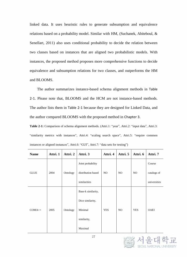
The author summarizes instance-based schema alignment methods in Table
2-1. Please note that, BLOOMS and the HCM are not instance-based methods.
The author lists them in Table 2-1 because they are designed for Linked Data, and
the author compared BLOOMS with the proposed method in Chapter 3.
Table 2-1: Comparison of schema alignment methods. (Attri.1: “year”, Attri.2: “input data”, Attri.3:
“similarity metrics with instances”, Attri.4: “scaling search space”, Attri.5: “require common
instances or aligned instances”, Attri.6: “GUI”, Attri.7: “data sets for testing”)
Name Attri. 1 Attri. 2 Attri. 3 Attri. 4 Attri. 5 Attri. 6 Attri. 7
GLUE 2004 Ontology
Joint probability
distribution based
similarities
NO NO NO
Course
catalogs of
universities
COMA++ 2005 Ontology
Base-k similarity,
Dice similarity,
Minimal
similarity,
Maximal
YES NO YES OAEI
28
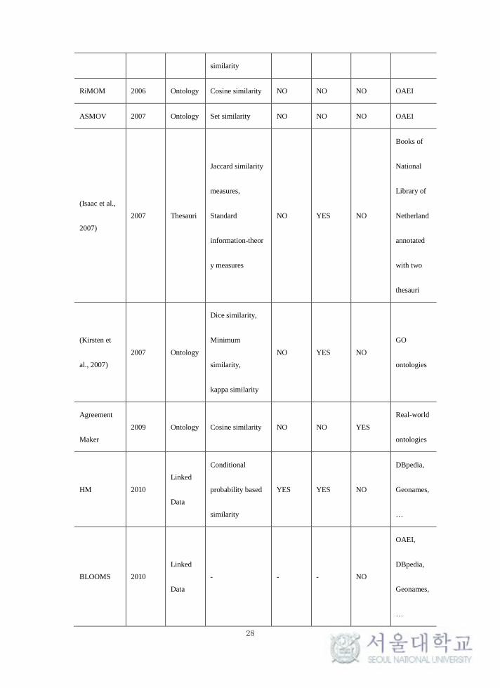
similarity
RiMOM 2006 Ontology Cosine similarity NO NO NO OAEI
ASMOV 2007 Ontology Set similarity NO NO NO OAEI
(Isaac et al.,
2007)
2007 Thesauri
Jaccard similarity
measures,
Standard
information-theor
y measures
NO YES NO
Books of
National
Library of
Netherland
annotated
with two
thesauri
(Kirsten et
al., 2007)
2007 Ontology
Dice similarity,
Minimum
similarity,
kappa similarity
NO YES NO
GO
ontologies
Agreement
Maker
2009 Ontology Cosine similarity NO NO YES
Real-world
ontologies
HM 2010
Linked
Data
Conditional
probability based
similarity
YES YES NO
DBpedia,
Geonames,
…
BLOOMS 2010
Linked
Data
- - - NO
OAEI,
DBpedia,
Geonames,
…
29
(Suchanek et
al., 2011)
2011
Linked
Data
Conditional
probability based
similarity
NO NO NO
DBpedia,
YAGO
HCM 2012
Linked
Data
- - - NO
OAEI
Billion
Triple
Challenge
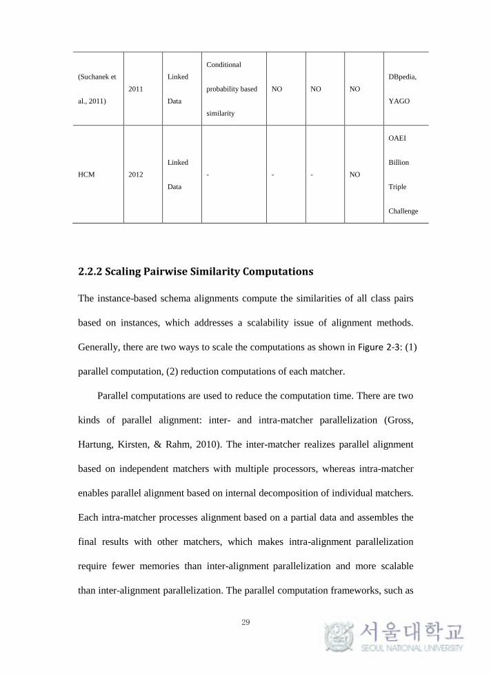
2.2.2 Scaling Pairwise Similarity Computations
The instance-based schema alignments compute the similarities of all class pairs
based on instances, which addresses a scalability issue of alignment methods.
Generally, there are two ways to scale the computations as shown in Figure 2-3: (1)
parallel computation, (2) reduction computations of each matcher.
Parallel computations are used to reduce the computation time. There are two
kinds of parallel alignment: inter- and intra-matcher parallelization (Gross,
Hartung, Kirsten, & Rahm, 2010). The inter-matcher realizes parallel alignment
based on independent matchers with multiple processors, whereas intra-matcher
enables parallel alignment based on internal decomposition of individual matchers.
Each intra-matcher processes alignment based on a partial data and assembles the
final results with other matchers, which makes intra-alignment parallelization
require fewer memories than inter-alignment parallelization and more scalable
than inter-alignment parallelization. The parallel computation frameworks, such as
30
MapReduce (Dean & Ghemawat, 2008), are used to find duplicates over massive
datasets (C. Wang et al., 2010), which can be used to decrease pair-wise similarity
computations in schema alignment. (Lin, 2009) and (Y. Wang, Metwally, &
Parthasarathy, 2013) use MapReduce to scale the similarity computations on
documents and entities that resemble instance-based schema alignment. (Tenschert
et al., 2009) introduces a workflow of ontology alignment based on MapReduce.
The V-Doc+ (Zhang, Hu, & Qu, 2012), PIDGIN (Wijaya, Talukdar, & Mitchell,
2013), and Parallel Ontology Bridge (Freckleton, 2013) scale the computations of
ontology alignment based on MapReduce.
Figure 2-3: Two strategies for scaling pairwise computations.
The second way is to reduce pairwise similarity computations of each
matcher, which is recognized as the problem of duplicate detection. This problem
is addressed by (Broder, Glassman, Manasse, & Zweig, 1997) to find duplicate
…
Input class pairs
Matcher 1
…
Results
Results
running time of matching process
Matcher 1 …Matcher 2 Matcher 3 Matcher m
…
running time of strategy 1
(parallel pairwise computation)
running time of strategy 2
(computation reduction of each matcher)
Matcher 1 Results
computations
reduction
Matcher 2
Matcher 3
Matcher mMatcher 2 Matcher 3 Matcher m
C1 C2
C1 Cm
…
Ci Cj
C1
…
31
Web pages. A Sketch that is a compressed Web document vector based on
min-wise independent permutations is used to represent a Web Document for
similarity computations. Similarly, the dimension of document vector can be
reduced by hashing functions reflecting to similarity computation functions in
Locality Sensitive Hashing (LSH) (Rajaraman & Ullman, 2011). These methods
are approximate duplicate detection. The LSH is adapted in (Duan et al., 2012) on
scaling instance-based schema alignment. The difference between the (Duan et al.,
2012) and the proposed method is that the IUT also considers the sequence for
pair-wise computations and limits the candidate pairs into the buckets created by
banding when using MinHash functions. The exact duplicate detection problem is
known as similarity join problem in the database community. Signatures
represented the original documents with a filtering phase to eliminate false
positives are used to match exact sets based on Hamming and Jaccard similarities
in PARTENUM and WTENUM (Arasu, Ganti, & Kaushik, 2006). The q-grams
are used to represented original text document, and the candidate pairs are
extracted based on prefix-filtering (Chaudhuri, Ganti, & Kaushik, 2006). For fast
navigate compared document, inverted index is also used in a prefix-filtering
based model in All-Pairs (Bayardo, Ma, & Srikant, 2007). For achieving better
performance, the PPjoin and PPjoin+ (Xiao, Wang, Lin, & Yu, 2008) use
positional and suffix filtering to eliminate candidate pairs. The PPjoin is adapted
into ontology alignment for scaling pairwise computations in HCM (Gruetze et al.,
2012).
32
2.2.3 Automatic Taxonomy Generation
With the rapid growth of large data sets in commercial, industrial, administrative
and other applications, the concept hierarchy generation has been studied from
1990s (Han, Cai, & Cercone, 1992; Piateski & Frawley, 1991). In an automatic
generated taxonomy, the data are organized with the concepts extracted from three
types of source data: (1) unstructured, (2) semi-structured, and (3) structured
(Hazman, El-Beltagy, & Rafea, 2011; Santoso, Haw, & Abdul-Mehdi, 2011). In
unstructured data, the terms are extracted based on Nature Language Processing
(NLP) methods, such as POS tagging (Drymonas, Zervanou, & Petrakis, 2010;
Knijff, Frasincar, & Hogenboom, 2013; Kummamuru, Lotlikar, Roy, Singal, &
Krishnapuram, 2004) or syntactic dependency (Cimiano, Hotho, & Staab, 2005).
The important ones are considered as the concepts with different metrics, such as
C/NC-value in (Drymonas et al., 2010), conditional probability, Pointwise Mutual
Information (PMI) and Resnik in (Cimiano et al., 2005), TF/IDF in (Brewster &
Wilks, 2004), domain pertinence and lexical cohesion in (Knijff et al., 2013).
Rather than a term, a concept can also be defined as a set of terms (Fung, Wang, &
Ester, 2003; Paukkeri, García-Plaza, Fresno, Unanue, & Honkela, 2012).
In semi-structured data and structured data, concepts are extracted from
schema with different transforming patterns. For example in XML, concepts can
be mapped from complexType (Bedini, Matheus, Patel-Schneider, Boran, &
Nguyen, 2011; Ferdinand, Zirpins, & Trastour, 2004; Ghawi & Cullot, 2009; J. Xu
& Li, 2007). Similar with XML, for databases, concepts can be mapped from
relations (Astrova, 2004; Cerbah, 2008; Lammari, Comyn-Wattiau, & Akoka,
33
2007). In contrast with these methods above, the proposed method in Chapter 5
does not use any complex machine learning algorithms or heuristic rules targeting
specific data to get concepts, but only extracts objects to form concepts, which is
lightweight and robust to be applied to any Linked Data set.
With the concepts established, taxonomies can be generated either with
heuristic rules based on features of data, such as extension and restriction in XML
(Bedini et al., 2011; Ghawi & Cullot, 2009) or different relationships in databases
(Cerbah, 2008; Lammari et al., 2007). Reference ontologies, such as WordNet
(Lee, Huh, & McNiel, 2008; Zheng, Borchert, & Kim, 2008), are also used to
build taxonomies. Nevertheless, the most popular methods are based on
probabilistic models and can be classified into two kinds:
(a) Fill the taxonomy with the established concepts and new discovered concepts.
The most traditional methods of this kind use the established concepts as leaf
nodes and create stem nodes with them. The hierarchical clustering algorithms
known as agglomerative UPGMA and bisecting k-means (A. K. Jain & Dubes,
1988) are frequently used. And the bisecting k-means is considered a better
solution than UPGMA (Steinbach, Karypis, & Kumar, 2000). However, it is
inflexible to use these methods that need to set parameters, such as the number of
clusters for k-means. The established concepts are not only used as leafs but also
used as stems. The Formal Concept Analysis (FCA) uses a set of terms as
intensions of a concept, and builds a taxonomy with these concepts (Cimiano et al.,
2005; Drymonas et al., 2010). The Self-Organizing Map (SOM) is also used to
reduce the dimensions of data (instances) features into SOM neurons for clustering
34
data at each level of a taxonomy (Paukkeri et al., 2012). Different with the
proposed method in Chapter 5, these methods focus on building a hierarchical
structure for organizing instances, but with little consideration of the concept
interpretation or labeling. For example, in the experiment in Section 5.6, FCA
obtains low precision for generating meaningless concepts that have common
instances.
(b) Fill the taxonomy only with the established concepts.
The methods of this kind build a taxonomy only with already established concepts.
The relation between two concepts is mostly defined with a similarity measure.
The Subsumption (Sanderson & Croft, 1999) is used to determine a subsumption
relation between two concepts, and is considered as one of the most classical
methods for concept hierarchy generation. Studies, such as (Schmitz, 2006) and
(Knijff et al., 2013), improve the subsumption-based approaches for different
usages. Other studies are inspired to boost the precision of the subsumption-based
method by using probability models. Some of them try to improve the precision by
developing more advanced metrics to compute the importance of a concept, such
as topicality and predictiveness in DSP (Lawrie & Croft, 2003), hierarchy
coverage and concept distinctiveness in DisCover (Kummamuru et al., 2004). To
build a taxonomy for social tags, the EXT (Heymann & Garcia-Molina, 2006) is
introduced as a high efficient and effective extensible greedy algorithm that places
concepts ordered with importance of a similarity graph into a hierarchy based on a
similarity measure. Furthermore, the EXT is improved by modifying the greedy
algorithm into a Directed Acyclic Graph (DAG) allocation algorithm (Eda,
35
Yoshikawa, Uchiyama, & Uchiyama, 2009) or by changing the sorting algorithm
and similarity measure in the IUT (Zong et al., 2015).
The proposed method in Chapter 5 combines the IUT and Subsumption to
generate a taxonomy based on the concept defined. In an addition, the proposed
method further decreases the computations by removing the redundant instances
and objects, and refines a generated taxonomy with these removed instances and
objects. These mechanism guarantees both the efficiency and effectiveness on
taxonomy construction. In contrast with the existing methods, with the multiple
features of Linked Data, the proposed method adapts automatic taxonomy
generation methods to build diverse taxonomies in different facets. To the best of
the author’s knowledge, this is the first study that realizes generation of faceted
taxonomy automatically in Linked Data.
36
3 Aligning Schemas with Subsumption and
Equivalence Relations
3.1 Introduction
In this chapter, the author proposes a new Instance-based Unified Taxonomy
generation algorithm called IUT for aligning ontology in Linked Data. The
taxonomy used in this chapter is defined in general, which contains two relations,
subsumption and equivalence, and supports multiple inheritance. The content of
this chapter is based on the author’s previous work published (Zong et al., 2015).
The IUT adapts the EXT (Heymann & Garcia-Molina, 2006), an algorithm that
builds a taxonomy for social tags originally and can be used for generating ontology
for RDF resources in the work (Nansu, Sungin, & Hong-Gee, 2013). The IUT uses a
unified graph to restrict the alignment search space, which is proved to be capable
of finding more suitable pairs to be compared instead of using all the combinations
of instances. The author tests the IUT with two data sets, DBpedia and YAGO2 in
LOD, and evaluates the results with gold standards. Four tasks, intra-subsumption
in DBpedia (DBpedia-DBpedia), and YAGO2 (YAGO2-YAGO2),
inter-subsumption and equivalence between DBpedia and YAGO2
(YAGO2-DBpedia), are designed to discover two kinds of relations, subsumption
and equivalence. The author compares the IUT with two other state-of-the-art
methods (the Heuristic Mapper (HM) (Parundekar et al., 2010) and BLOOMS (P.
Jain et al., 2010)), and the experiments show that the IUT outperforms the existing
ontology alignment algorithms. Three main reasons for failures of instance-based
37
ontology alignment in LOD, which are (1) insufficient taxonomic description on the
instance level, (2) multi-instantiation, and (3) different taxonomic structure of
ontologies, are also discussed.
The rest of this chapter is organized as follows: Section 3.2 gives a formal
problem definition; Section 3.3 details on the methodology of the proposed method;
in Section 3.4 and 3.5, the author demonstrates the results of the proposed method;
Section 3.6 discusses limitations of this study, and the conclusions are presented in
Section 3.7.
38
3.2 Problem Definition
Figure 3-1: A data example for ontology alignment.
In order to help readers understand this paper, the author uses an ongoing example
in Figure 3-1 to explain the problem of schema alignment and the process of the
proposed method. The author uses two ontologies as input data. That is the one
shaped in solid line from DBpedia Ontology containing five classes
(“ 𝑐1: 𝐿𝑒𝑔𝑎𝑙𝐴𝑐𝑡𝑜𝑟 ”, “ 𝑐2: 𝑃𝑒𝑟𝑠𝑜𝑛 ”, “ 𝑐3: 𝑂𝑟𝑔𝑎𝑛𝑖𝑧𝑎𝑡𝑖𝑜𝑛 ”, “ 𝑐4: 𝐺𝑒𝑛𝑒𝑟𝑎𝑙 ”, and
“ 𝑐5: 𝐴𝑟𝑡𝑖𝑠𝑡 ”) and four instances (“ 𝑖1_1: 𝐺𝑎𝑛𝑛𝑦𝑠 ”, “ 𝑖2_1: 𝐵𝑎𝑠ℎ𝑦 ”,
“𝑖3_1: 𝐷𝑜𝑢𝑏𝑙𝑒_𝑂(𝑐ℎ𝑎𝑟𝑖𝑡𝑦)”, and “𝑖4_1: 𝑃𝑎𝑡𝑟𝑖𝑐𝑘_𝐻𝑢𝑠𝑒”). And the other one shaped
in dotted line from YAGO2 contains three classes (“𝑐6: 𝐴𝑔𝑒𝑛𝑡”, “𝑐7: 𝑃𝑒𝑜𝑝𝑙𝑒”, and
“ 𝑐8: 𝐺𝑟𝑜𝑢𝑝 ”) and three instances (“ 𝑖1_2: 𝐺𝑎𝑛𝑛𝑦𝑠 ”, “ 𝑖2_2: 𝐵𝑎𝑠ℎ𝑦 ”, and
“ 𝑖3_2: 𝐷𝑜𝑢𝑏𝑙𝑒_𝑂(𝑐ℎ𝑎𝑟𝑖𝑡𝑦) ”) (the author changed the original ontologies to
simplify the example used). The classes belonging to the same ontology are
connected with the intra-subsumption relations. For example, “𝑐2: 𝑃𝑒𝑟𝑠𝑜𝑛” is a
sub-class of “𝑐1: 𝐿𝑒𝑔𝑎𝑙𝐴𝑐𝑡𝑜𝑟” in the first ontology. Schema alignment is the
process of discovering correspondences that include subsumption and equivalence
relations between classes from multiple ontologies. The author adapts the
C1:
Legal Actor
C2:
Person
C5:ArtistC4: General
I2_1: BashyI1_1: Gannys
C3: Organization
I4_1:
Patrick_Huse
I3_1:
Double_O(charity)
C6: Agent
C7:
People
I1_2: Gannys
C8:Group
I3_2:
Double_O(charity)
sameAs
I2_2: Bashy
sameAs
sameAs
Class of Dbpedia ontology Class of YAGO2 Instance
39
conditions for an instance-based schema alignment that instances are aligned with
“Owl:sameAS” to other instances from different ontologies. The author defines the
problem in more detail as follows:
Input: Given two ontologies, a source ontology 𝑂1(𝐶1, 𝐼1) and a target ontology
𝑂2(𝐶2, 𝐼2) , where 𝑂1(𝐶1, 𝐼1) contains a class set 𝐶1 = {𝑐1, 𝑐2, … , 𝑐𝑘} and an
instance set 𝐼1 = {𝑖1, 𝑖2, … , 𝑖𝑙} , and 𝑂2(𝐶2, 𝐼2) contains a class set 𝐶2 =
{𝑐𝑘+1, 𝑐𝑘+2, … , 𝑐𝑚} and an instance set 𝐼2 = {𝑖𝑙+1, 𝑖𝑙+2, … , 𝑖𝑛′}. The two instance
sets are mapped by “Owl:sameAs”. For example, instance “𝑖1_1: 𝐺𝑎𝑛𝑛𝑦𝑠” from 𝐶1
is same with “𝑖1_2: 𝐺𝑎𝑛𝑛𝑦𝑠” from 𝐶2 . Each class 𝑐𝑖 in 𝐶1 or 𝐶2 contains an
instance set 𝐼𝑐𝑖, where each element is corresponding to the element in the instance
set 𝐼1 or 𝐼2. The instance set 𝐼𝑐𝑖 for class 𝑐𝑖 follows the common extension (Isaac
et al., 2007) to describe the taxonomic information of 𝑐𝑖 in 𝐶1 or 𝐶2, which is that
𝑐𝑖 contains all the instances of 𝑐𝑗 if 𝑐𝑖 is the super class of 𝑐𝑗. For example in
Figure 3-1, 𝐼𝑐2:𝑃𝑒𝑟𝑠𝑜𝑛 = {“𝑖2_1: 𝐵𝑎𝑠ℎ𝑦”, “𝑖1_1: 𝐺𝑎𝑛𝑛𝑦𝑠”, “𝑖4_1: 𝑃𝑎𝑡𝑟𝑖𝑐_𝐻𝑢𝑠𝑒”}
contains the instance “𝑖2_1: 𝐵𝑎𝑠ℎ𝑦” because “𝑐2: 𝑃𝑒𝑟𝑠𝑜𝑛” is the super class of
“𝑐5: 𝐴𝑟𝑡𝑖𝑠𝑡” that has the instance set 𝐼𝑐5:𝐴𝑟𝑡𝑖𝑠𝑡 = {“𝑖2_1: 𝐵𝑎𝑠ℎ𝑦”}.
Output: A set of mappings 𝐴 = {𝑎1, 𝑎2, … , 𝑎𝑘} is the output of the alignment
processing. Each mapping 𝑎𝑖 = (𝑐𝑒 , 𝑐𝑓 , 𝑟𝑖) contains three elements, where 𝑐𝑒 ∈ 𝐶1,
𝑐𝑓 ∈ 𝐶2, and 𝑟𝑖 can be a subsumption or equivalence relation.
The subsumption relations are directly determined instead of being deduced by a
reasoning mechanism based on equivalence relations and existing
intra-subsumptions, otherwise the generated subsumption relations are not
independent and can be affected by the equivalence relations (Spiliopoulos et al.,

40
2010). For example, the class “𝑐1: 𝐿𝑒𝑔𝑎𝑙𝐴𝑐𝑡𝑜𝑟” from 𝐶1 should not be considered
equivalent as the class “𝑐6: 𝐴𝑔𝑒𝑛𝑡” from 𝐶2 if the relation is deduced by the facts
that (1) “𝑐1: 𝐿𝑒𝑔𝑎𝑙𝐴𝑐𝑡𝑜𝑟” is the super class of “𝑐2: 𝑃𝑒𝑟𝑠𝑜𝑛” and (2) “𝑐6: 𝐴𝑔𝑒𝑛𝑡” is
the super class of “𝑐7: 𝑃𝑒𝑜𝑝𝑙𝑒”, and (3) a new established relation that “𝑐2: 𝑃𝑒𝑟𝑠𝑜𝑛”
is equivalent to “𝑐7: 𝑃𝑒𝑜𝑝𝑙𝑒”.
41
3.3 Methods
3.3.1 Workflow of Instance-based Schema Alignment
Figure 3-2: Workflow of instance-based schema alignment with the IUT.
The IUT is a unified taxonomy generation algorithm that generates alignments for a
source ontology and a target ontology based on a virtual graph generated by using
the common instances shared in two classes from the two ontologies. Figure 3-2
shows the workflow of the IUT. The procedure of aligning is separated into two
parts: instance-class matrix generation, and subsumption and equivalence relations
generation. In first part, the input data will be converted into an instance-class
matrix, and the matrix will be used to build a virtual graph based on the aligned
instances in the second part. The subsumption and equivalence relations are
extracted from the virtual graph after the virtual graph is established.
Source ontology and Target
ontology
Common Instances Scoping
Common Instances Generation
Instance-Class Matrix Generation
Class-relation multi-graph
Generation
Instance-Class Matrix
Input
Virtual Graph Generation
Alignments
Output
instance-class matrix generation
subsumption and equivalence
relations generation
42
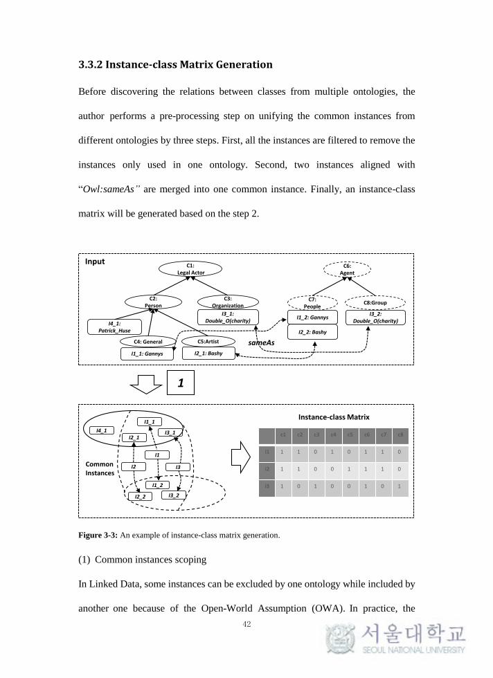
3.3.2 Instance-class Matrix Generation
Before discovering the relations between classes from multiple ontologies, the
author performs a pre-processing step on unifying the common instances from
different ontologies by three steps. First, all the instances are filtered to remove the
instances only used in one ontology. Second, two instances aligned with
“Owl:sameAs” are merged into one common instance. Finally, an instance-class
matrix will be generated based on the step 2.
Figure 3-3: An example of instance-class matrix generation.
(1) Common instances scoping
In Linked Data, some instances can be excluded by one ontology while included by
another one because of the Open-World Assumption (OWA). In practice, the
C1:Legal Actor
C2:Person
C5:ArtistC4: General
I2_1: BashyI1_1: Gannys
C3:Organization
I4_1:Patrick_Huse
I3_1:Double_O(charity)
C6:Agent
C7:People
I1_2: Gannys
C8:Group
I3_2:Double_O(charity)
Input
sameAs
c1 c2 c3 c4 c5 c6 c7 c8
i1 1 1 0 1 0 1 1 0
i2 1 1 0 0 1 1 1 0
i3 1 0 1 0 0 1 0 1
Instance-class Matrix
I2_2: Bashy
I4_1I2_1
I1_1
I3_1
I2_2
I1_2
I3_2
I1
I2 I3CommonInstances
1
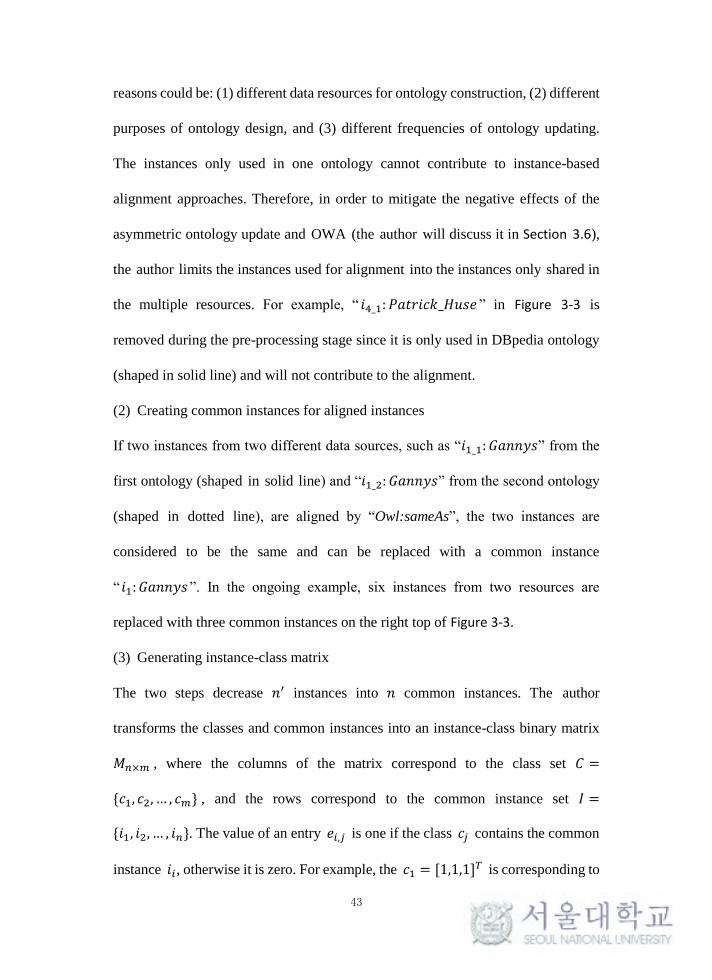
43
reasons could be: (1) different data resources for ontology construction, (2) different
purposes of ontology design, and (3) different frequencies of ontology updating.
The instances only used in one ontology cannot contribute to instance-based
alignment approaches. Therefore, in order to mitigate the negative effects of the
asymmetric ontology update and OWA (the author will discuss it in Section 3.6),
the author limits the instances used for alignment into the instances only shared in
the multiple resources. For example, “ 𝑖4_1: 𝑃𝑎𝑡𝑟𝑖𝑐𝑘_𝐻𝑢𝑠𝑒 ” in Figure 3-3 is
removed during the pre-processing stage since it is only used in DBpedia ontology
(shaped in solid line) and will not contribute to the alignment.
(2) Creating common instances for aligned instances
If two instances from two different data sources, such as “𝑖1_1: 𝐺𝑎𝑛𝑛𝑦𝑠” from the
first ontology (shaped in solid line) and “𝑖1_2: 𝐺𝑎𝑛𝑛𝑦𝑠” from the second ontology
(shaped in dotted line), are aligned by “Owl:sameAs”, the two instances are
considered to be the same and can be replaced with a common instance
“ 𝑖1: 𝐺𝑎𝑛𝑛𝑦𝑠”. In the ongoing example, six instances from two resources are
replaced with three common instances on the right top of Figure 3-3.
(3) Generating instance-class matrix
The two steps decrease 𝑛′ instances into 𝑛 common instances. The author
transforms the classes and common instances into an instance-class binary matrix
𝑀𝑛×𝑚 , where the columns of the matrix correspond to the class set 𝐶 =
{𝑐1, 𝑐2, … , 𝑐𝑚} , and the rows correspond to the common instance set 𝐼 =
{𝑖1, 𝑖2, … , 𝑖𝑛}. The value of an entry 𝑒𝑖,𝑗 is one if the class 𝑐𝑗 contains the common
instance 𝑖𝑖, otherwise it is zero. For example, the 𝑐1 = [1,1,1]𝑇 is corresponding to
44
the fact that the class “𝑐1: 𝐿𝑒𝑔𝑎𝑙𝐴𝑐𝑡𝑜𝑟” contains three instances “𝑖1: 𝐺𝑎𝑛𝑛𝑦𝑠”,
“𝑖2: 𝐵𝑎𝑠ℎ𝑦”, and “𝑖3: 𝐷𝑜𝑢𝑏𝑙𝑒_𝑂(𝑐ℎ𝑎𝑟𝑖𝑡𝑦)” in Figure 3-3.
3.3.3 Subsumption and Equivalence Relations Discovering
The alignment is processed by the following steps based on the instance-class
matrix generated: first, the classes in the matrix are sorted in descending order by
the degrees in a class-relation multi-graph 𝐺(𝐸, 𝑉); second, the sorted classes are
put onto the right position in a virtual graph. The subsumption and equivalence
relations are used to form the virtual graph.
(1) Class-relation multi-graph generation
For a class-relation multi-graph 𝐺(𝐸, 𝑉), all the classes 𝐶 = {𝑐1, 𝑐2, … , 𝑐𝑚} are put
into the 𝐺(𝐸, 𝑉), and each class 𝑐𝑖 is a vertex 𝑣𝑖. For each pair of vertices 𝑐𝑖 and
𝑐𝑗 , |𝑐𝑜𝑚𝑚𝑜𝑛𝐼𝑛𝑠𝑡𝑎𝑛𝑐𝑒𝑠(𝑐𝑖 , 𝑐𝑗)| number of links between 𝑐𝑖 and 𝑐𝑗 are built,
where |𝑐𝑜𝑚𝑚𝑜𝑛𝐼𝑛𝑠𝑡𝑎𝑛𝑐𝑒𝑠(𝑐𝑖 , 𝑐𝑗)| is the cardinality of the common instances set
of 𝑐𝑖 and 𝑐𝑗.
For example, |𝑐𝑜𝑚𝑚𝑜𝑛𝐼𝑛𝑠𝑡𝑎𝑛𝑐𝑒𝑠(“𝑐1: 𝐿𝑒𝑔𝑎𝑙𝐴𝑐𝑡𝑜𝑟”, “𝑐𝑗: 𝐴𝑔𝑒𝑛𝑡”)| = 3 in
the ongoing example.
(2) Virtual graph generation
The vertices (classes) are sorted in descending order by the degrees and are put into
a queue 𝑄. In each iteration, a class is de-queued and put onto the right position by
computing the relation with existing classes in the virtual graph using the following
definitions:
45
Definition 3-1. Subsumption: For a pair of vertices 𝑐𝑖 and 𝑐𝑗, where 𝑐𝑖 originates
from either one of the two ontologies (source and target) and 𝑐𝑗 from the other
ontology, if 𝑠𝑢𝑏(𝑐𝑖, 𝑐𝑗) ≥ 𝜒𝑠 , then 𝑐𝑖 is considered as the subclass of 𝑐𝑗 . The
𝑠𝑢𝑏(𝑐𝑖 , 𝑐𝑗) is computed by:
𝑠𝑢𝑏(𝑐𝑖, 𝑐𝑗) =|𝑐𝑜𝑚𝑚𝑜𝑛𝐼𝑛𝑠𝑡𝑎𝑛𝑐𝑒(𝑐𝑖,𝑐𝑗)|
|𝑐𝑖| (3.1)
Definition 3-2. Equivalence: For a pair of vertices 𝑐𝑖 and 𝑐𝑗, where 𝑐𝑖 originates
from either one of the two ontologies (source and target) and 𝑐𝑗 from the other
ontology, if 𝑠𝑢𝑏(𝑐𝑖, 𝑐𝑗) ≥ 𝜒𝑠 and 𝑠𝑢𝑏(𝑐𝑗, 𝑐𝑖) ≥ 𝜒𝑠 , then 𝑐𝑖 is considered
equivalent to 𝑐𝑗.
In practice, if the above mentioned two definitions are not satisfied, the author will
further compute a supplementary definition for equivalence by Jaccard similarity.
Definition 3-3. Equivalence (supplementary): For a pair of vertices 𝑐𝑖 and 𝑐𝑗,
where 𝑐𝑖 originates from either one of the two ontologies (source and target) and 𝑐𝑗
from the other ontology, if 𝑠𝑖𝑚(𝑐𝑖, 𝑐𝑗) ≥ 𝜒𝑒, then 𝑐𝑖 is considered equivalent to 𝑐𝑗.
The 𝑠𝑖𝑚(𝑐𝑖, 𝑐𝑗) is computed by Jaccard similarity shown as follows:
𝑠𝑖𝑚(𝑐𝑖, 𝑐𝑗) =|𝑐𝑜𝑚𝑚𝑜𝑛𝐼𝑛𝑠𝑡𝑎𝑛𝑐𝑒(𝑐𝑖,𝑐𝑗)|
|𝑐𝑖|+|𝑐𝑗|−|𝑐𝑜𝑚𝑚𝑜𝑛𝐼𝑛𝑠𝑡𝑎𝑛𝑐𝑒(𝑐𝑖,𝑐𝑗)| (3.2)
For a new added vertex, if the relation with an existing vertex is equivalence, an
inbound edge and outbound edge of the vertex will be added to the existing vertex.
If a new added vertex has multiple subsumption relations with the existing vertices
(ancestors), the outbound edges of the vertex will be added to the super-vertices
that is an ancestor without a path from any other ancestor. The relations between
classes in the unified graph contain the new discovered relations and the original

46
existing relations. We return the new discovered relations as the alignments. The
details of the process of the IUT are shown in Algorithm 3-1.
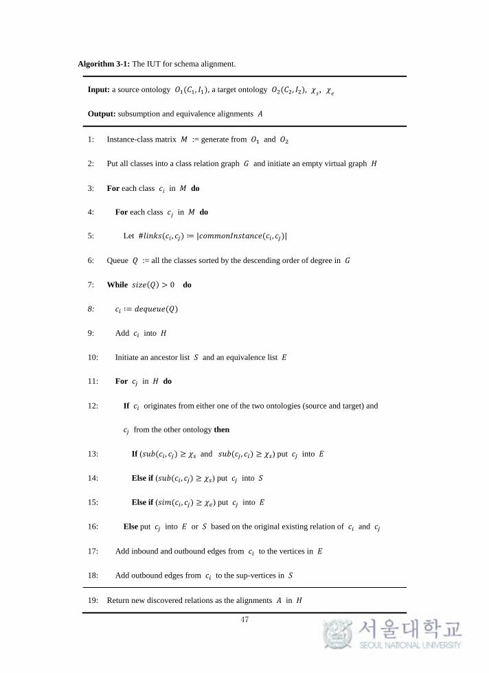
47
Algorithm 3-1: The IUT for schema alignment.
Input: a source ontology 𝑂1(𝐶1, 𝐼1), a target ontology 𝑂2(𝐶2, 𝐼2), 𝜒𝑠, 𝜒𝑒
Output: subsumption and equivalence alignments 𝐴
1: Instance-class matrix 𝑀 := generate from 𝑂1 and 𝑂2
2: Put all classes into a class relation graph 𝐺 and initiate an empty virtual graph 𝐻
3: For each class 𝑐𝑖 in 𝑀 do
4: For each class 𝑐𝑗 in 𝑀 do
5: Let #𝑙𝑖𝑛𝑘𝑠(𝑐𝑖 , 𝑐𝑗) ≔ |𝑐𝑜𝑚𝑚𝑜𝑛𝐼𝑛𝑠𝑡𝑎𝑛𝑐𝑒(𝑐𝑖 , 𝑐𝑗)|
6: Queue 𝑄 := all the classes sorted by the descending order of degree in 𝐺
7: While 𝑠𝑖𝑧𝑒(𝑄) > 0 do
8: 𝑐𝑖 ∶= 𝑑𝑒𝑞𝑢𝑒𝑢𝑒(𝑄)
9: Add 𝑐𝑖 into 𝐻
10: Initiate an ancestor list 𝑆 and an equivalence list 𝐸
11: For 𝑐𝑗 in 𝐻 do
12: If 𝑐𝑖 originates from either one of the two ontologies (source and target) and
𝑐𝑗 from the other ontology then
13: If (𝑠𝑢𝑏(𝑐𝑖 , 𝑐𝑗) ≥ 𝜒𝑠 and 𝑠𝑢𝑏(𝑐𝑗 , 𝑐𝑖) ≥ 𝜒𝑠) put 𝑐𝑗 into 𝐸
14: Else if (𝑠𝑢𝑏(𝑐𝑖 , 𝑐𝑗) ≥ 𝜒𝑠) put 𝑐𝑗 into 𝑆
15: Else if (𝑠𝑖𝑚(𝑐𝑖 , 𝑐𝑗) ≥ 𝜒𝑒) put 𝑐𝑗 into 𝐸
16: Else put 𝑐𝑗 into 𝐸 or 𝑆 based on the original existing relation of 𝑐𝑖 and 𝑐𝑗
17: Add inbound and outbound edges from 𝑐𝑖 to the vertices in 𝐸
18: Add outbound edges from 𝑐𝑖 to the sup-vertices in 𝑆
19: Return new discovered relations as the alignments 𝐴 in 𝐻
48
3.4 Experiments
The author implemented the proposed method based on JDK 1.6 using an Intel
I7-2600 CPU with 16 GB RAM on Windows 8 64 bit version.
3.4.1 Schema Alignment Algorithms in Comparison
The author compared the IUT with two state-of-the-art methods: the HM
(Parundekar et al., 2010) that is an instance-based alignment method and BLOOMS
(P. Jain et al., 2010) that is a lexical- and structure-based method.
For the HM, the author used the threshold (min=0.01 max=0.90) as mentioned
in (Parundekar et al., 2010). For BLOOMS, the author downloaded the source code
from the website ("BLOOMS,") and used the WordNet 2.1 ("WordNet,") as the
thesauri. (The reason why the author did not use Wikipedia is that too much time is
spent to send the request to the server, which makes the computation not feasible).
3.4.2 Data and Experiment Design
In ontology alignment, comparison of alignment methods should be based on an
identical evaluation scenario, a standardized set of tests serving as a basis for
comparison (Bellahsene et al., 2011). However, as far as we know, there lacks
benchmarks for measuring the efficiency and effectiveness of the LOD schema
alignment methods. The author decided to build the test data sets based on the most
famous ontology in LOD that supplies both taxonomic structure and rich instances.
Furthermore, the author chose the gold standards either used in the existing
schema-matching projects or created manually as the expected mappings for the
tests. The author gained the study population, with instance size ranged from 0 to
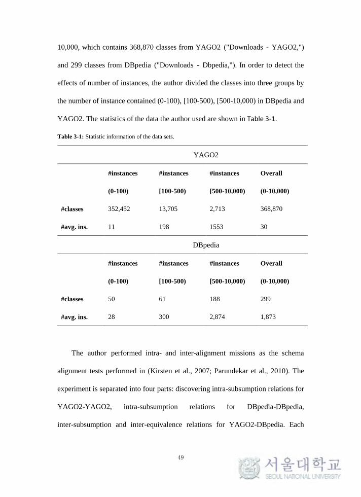
49
10,000, which contains 368,870 classes from YAGO2 ("Downloads - YAGO2,")
and 299 classes from DBpedia ("Downloads - Dbpedia,"). In order to detect the
effects of number of instances, the author divided the classes into three groups by
the number of instance contained (0-100), [100-500), [500-10,000) in DBpedia and
YAGO2. The statistics of the data the author used are shown in Table 3-1.
Table 3-1: Statistic information of the data sets.
YAGO2
#instances
(0-100)
#instances
[100-500)
#instances
[500-10,000)
Overall
(0-10,000)
#classes 352,452 13,705 2,713 368,870
#avg. ins. 11 198 1553 30
DBpedia
#instances
(0-100)
#instances
[100-500)
#instances
[500-10,000)
Overall
(0-10,000)
#classes 50 61 188 299
#avg. ins. 28 300 2,874 1,873
The author performed intra- and inter-alignment missions as the schema
alignment tests performed in (Kirsten et al., 2007; Parundekar et al., 2010). The
experiment is separated into four parts: discovering intra-subsumption relations for
YAGO2-YAGO2, intra-subsumption relations for DBpedia-DBpedia,
inter-subsumption and inter-equivalence relations for YAGO2-DBpedia. Each
50
alignment method is measured for each task in terms of its running time (efficiency)
and F-measure (effectiveness) (Bellahsene et al., 2011).
(1) For YAGO2-YAGO2, the classes with the cardinality of the instances set
ranging from 0 to 10,000 in the YAGO2 are used to generate intra-subsumption
relations between classes, and the relations are evaluated by the YAGO Taxonomy
("Downloads - YAGO2,").
(2) Similar to YAGO2-YAGO2, intra-subsumption relations in DBpedia-DBpedia
are generated based on the DBpedia classes with the same cardinality range
(0-10,000) and are evaluated by DBpedia Ontology ("Downloads - Dbpedia,").
(3) For YAGO2-DBpedia, the same DBpedia and YAGO2 classes used in the
previous two experiments are adopted. In order to create common instances shared
by the classes from DBpedia and YAGO2, the YAGO2-DBpedia
instances-mapping file downloaded from DBpedia 3.9 was used. For example,
through the “Owl:sameAs” mapping for the instance
“YAGO:ESF_Men's_Championship” contained by a YAGO2 class
“YAGO:SoftballChampionships” and the instance
“DBpedia:ESF_Men's_Championship” contained by a DBpedia class
“DBPedia:SoftballLeague”, can consider that “YAGO:SoftballChampionships” and
“DBPedia:SoftballLeague” contain a same instance “ESF_Men's_Championship”
that represents “YAGO:ESF_Men's_Championship” and
“DBpedia:ESF_Men's_Championship”. The subsumption relations are evaluated
by the gold standard used in the PARIS ("Subsumption alignment of YAGO2 and
Dbpedia,"). The equivalence relations are evaluated by the gold standard that is

51
manually created in NetEstate ("Ontology matching for classes in YAGO and
DBpedia ontologies," 2014). In order to compute the recall, the classes needed to be
aligned are limited into the classes existing in the gold standard instead of using all
the classes in two data sets.
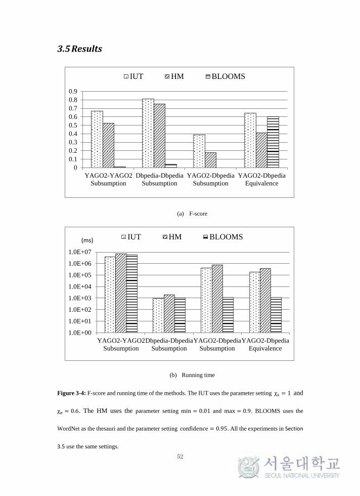
52
3.5 Results
(a) F-score
(b) Running time
Figure 3-4: F-score and running time of the methods. The IUT uses the parameter setting χs = 1 and
χe = 0.6. The HM uses the parameter setting min = 0.01 and max = 0.9. BLOOMS uses the
WordNet as the thesauri and the parameter setting confidence = 0.95. All the experiments in Section
3.5 use the same settings.
0
0.1
0.2
0.3
0.4
0.5
0.6
0.7
0.8
0.9
YAGO2-YAGO2
Subsumption
Dbpedia-Dbpedia
Subsumption
YAGO2-Dbpedia
Subsumption
YAGO2-Dbpedia
Equivalence
IUT HM BLOOMS
1.0E+00
1.0E+01
1.0E+02
1.0E+03
1.0E+04
1.0E+05
1.0E+06
1.0E+07
YAGO2-YAGO2
Subsumption
Dbpedia-Dbpedia
Subsumption
YAGO2-Dbpedia
Subsumption
YAGO2-Dbpedia
Equivalence
IUT HM BLOOMS(ms)
53
Figure 3-4 shows the overall (0-10,000) results of the three methods for four
alignment experiments. The IUT is the fastest algorithm for two intra-alignment
tasks (968 (ms) for DBpedia-DBpedia intra-subsumption and 3,981,676 (ms) for
YAGO2-YAGO2 intra-subsumption), since an instance-based approach is more
efficient for large classes. BLOOMS is the fastest algorithm for the two
inter-alignment tasks (1,197 (ms) for YAGO2-DBpedia inter-subsumption and
1,205 (ms) for YAGO2-DBpedia inter-equivalence), since BLOOMS ignores the
comparison of the instance sets, which is very expensive. However, BLOOMS fails
inter-subsumption alignment but achieves a good result for inter-equivalence
alignment (0.599). The IUT achieves the best F-score for all the alignment tasks
(0.666 for YAGO2-YAGO2 subsumption, 0.810 for DBpedia-DBpedia
subsumption, 0.388 for YAGO2-DBpedia subsumption, and 0.641 for
YAGO2-DBpedia equivalence) within a relatively reasonable time. The author
introduces the experiments results in detail in the next sub-sections.
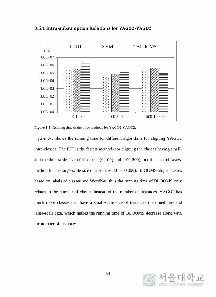
54
3.5.1 Intra-subsumption Relations for YAGO2-YAGO2
Figure 3-5: Running time of the three methods for YAGO2-YAGO2.
Figure 3-5 shows the running time for different algorithms for aligning YAGO2
intra-classes. The IUT is the fastest methods for aligning the classes having small-
and medium-scale size of instances (0-100) and [100-500), but the second fastest
method for the large-scale size of instances [500-10,000). BLOOMS aligns classes
based on labels of classes and WordNet, thus the running time of BLOOMS only
relates to the number of classes instead of the number of instances. YAGO2 has
much more classes that have a small-scale size of instances than medium- and
large-scale size, which makes the running time of BLOOMS decrease along with
the number of instances.
1.0E+00
1.0E+01
1.0E+02
1.0E+03
1.0E+04
1.0E+05
1.0E+06
1.0E+07
0-100 100-500 500-10000
IUT HM BLOOMS(ms)
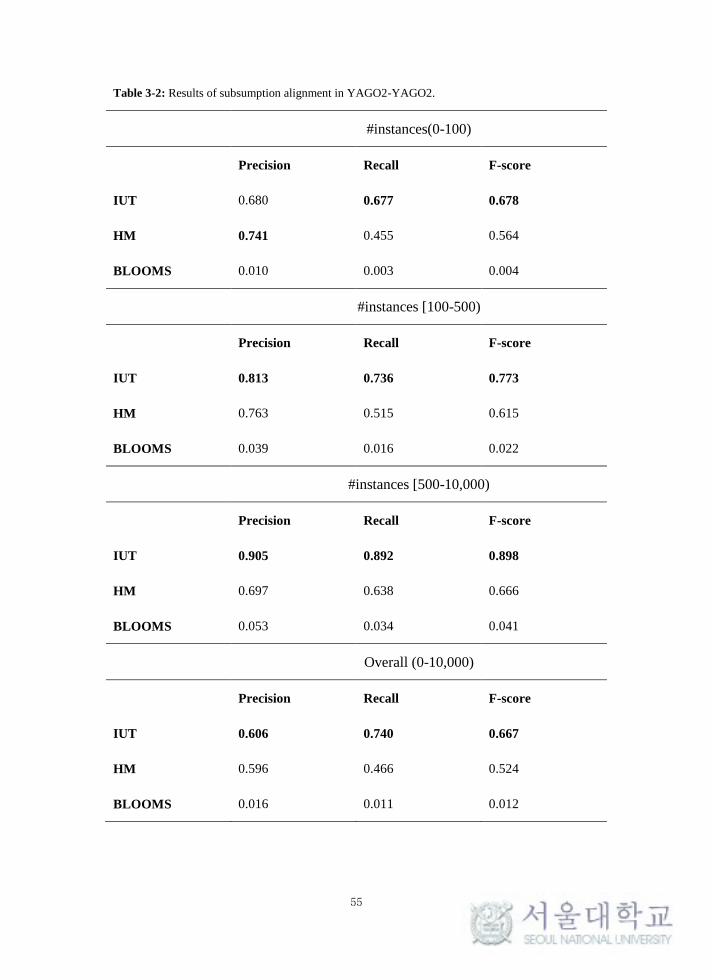
55
Table 3-2: Results of subsumption alignment in YAGO2-YAGO2.
#instances(0-100)
Precision Recall F-score
IUT 0.680 0.677 0.678
HM 0.741 0.455 0.564
BLOOMS 0.010 0.003 0.004
#instances [100-500)
Precision Recall F-score
IUT 0.813 0.736 0.773
HM 0.763 0.515 0.615
BLOOMS 0.039 0.016 0.022
#instances [500-10,000)
Precision Recall F-score
IUT 0.905 0.892 0.898
HM 0.697 0.638 0.666
BLOOMS 0.053 0.034 0.041
Overall (0-10,000)
Precision Recall F-score
IUT 0.606 0.740 0.667
HM 0.596 0.466 0.524
BLOOMS 0.016 0.011 0.012
56
Table 3-2 shows that the IUT obtains the most satisfactory F-score compared
with the other two approaches (0.678, 0.773, and 0.898). The results show the
lexical- and structure-based approach (BLOOMS) is unsuitable for discovering the
subsumption relations (0,004, 0.022, and 0.041). The subsumption relations are
more likely to be found by using instances than using lexical or structure
information. For example, the “YAGO:Hog110179649” contains eight instances
(“Russ Grimm”, “Jeff Bostic”, “Joe Jacoby”, “Rick Walker”, “Ken Huff”, “Don
Warren”, “George Starke”, “The Hogs (American football)”) and
“YAGO:SelfishPerson110576962” contains nine instances (“Russ Grimm”, “Jeff
Bostic”, “Joe Jacoby”, “Rick Walker”, “Ken Huff”, “Don Warren”, “George Starke”,
“The Hogs (American football)”, “Tufillo Triviño Tulio”). The instance-based
methods successfully discovered the subsumption relation between
“YAGO:Hog110179649” and “YAGO:SelfishPerson110576962”, but the
BLOOMS failed to find this relation since a hog can mean a greedy person but can
also mean a domesticated pig. However, some relations built are wrong by using
instance-based approaches, which are false positives and false negatives in F-score.
The author noticed two main reasons caused the false positives and false negatives
for intra-subsumption discovery: (1) insufficient description of taxonomy on the
instance level. A super class may have the same instances as its sub-class. For
example, “YAGO:Saber104121511” contains eight instances (“Swiss saber”,
“Szabla”, “Sabre de cavalerie légère modèle An IX”, “Sabre (fencing)”, “Sabre de
cuirassier modèle An IX”, “The French Connection (ice hockey)”, “Shashka”,
“Curved saber of San Martín”), and “YAGO:FencingSword103327691” contains
57
the exact same eight instances. The instance-based method got a wrong relation
(equivalence) since the two classes are same at the instance level. (2) multiple
instantiation. Instances may be assigned to multiple classes that have no relations
between each other. For example, “YAGO:ItalianBasses” containing one instance
(“Franco Calabrese”) has no connection with “YAGO:OperaticBasses” containing
three instances (“Charles Manners (bass)”, “Franco Calabrese”, “Alexandrov
Ensemble soloists”). However, the instance-based methods may discover a wrong
subsumption relation that “YAGO:ItalianBasses” is a sub-class of
“YAGO:OperaticBasses”. The author noticed that the 76.9% false positives and
false negatives are caused by the first reason.
Another phenomenon the author observed is that the F-score increases along
with the cardinality of instances sets of classes. Both the HM and the IUT get the
best F-score when using “500-10,000” data (0.666, 0.898). The author believes that
the more instances used for describing a class, the better the instances used can
represent the hierarchical structure of the class, which decreases the effects of the
first reason.
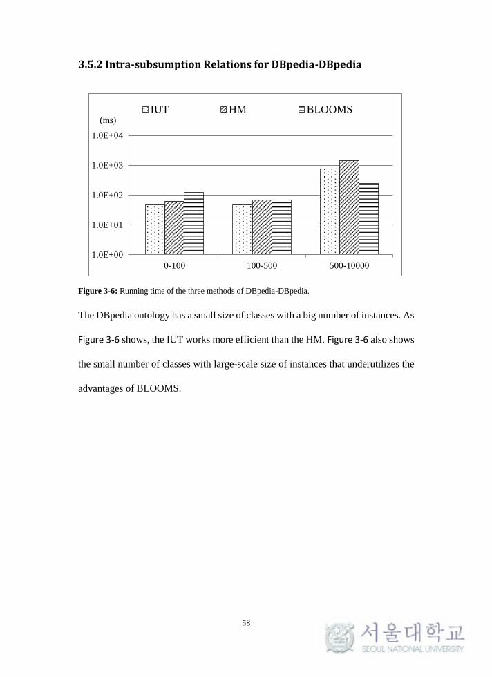
58
3.5.2 Intra-subsumption Relations for DBpedia-DBpedia
Figure 3-6: Running time of the three methods of DBpedia-DBpedia.
The DBpedia ontology has a small size of classes with a big number of instances. As
Figure 3-6 shows, the IUT works more efficient than the HM. Figure 3-6 also shows
the small number of classes with large-scale size of instances that underutilizes the
advantages of BLOOMS.
1.0E+00
1.0E+01
1.0E+02
1.0E+03
1.0E+04
0-100 100-500 500-10000
IUT HM BLOOMS(ms)
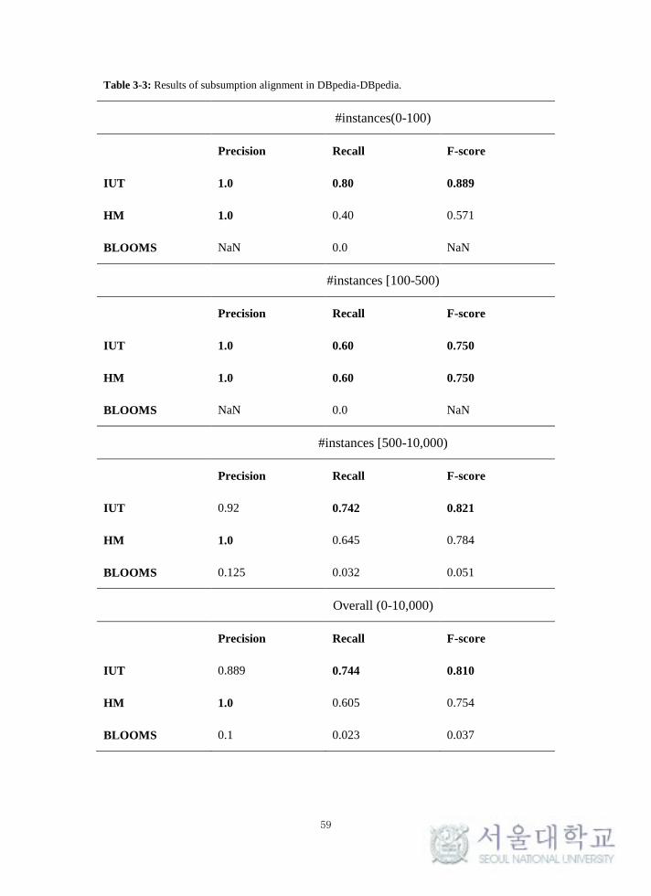
59
Table 3-3: Results of subsumption alignment in DBpedia-DBpedia.
#instances(0-100)
Precision Recall F-score
IUT 1.0 0.80 0.889
HM 1.0 0.40 0.571
BLOOMS NaN 0.0 NaN
#instances [100-500)
Precision Recall F-score
IUT 1.0 0.60 0.750
HM 1.0 0.60 0.750
BLOOMS NaN 0.0 NaN
#instances [500-10,000)
Precision Recall F-score
IUT 0.92 0.742 0.821
HM 1.0 0.645 0.784
BLOOMS 0.125 0.032 0.051
Overall (0-10,000)
Precision Recall F-score
IUT 0.889 0.744 0.810
HM 1.0 0.605 0.754
BLOOMS 0.1 0.023 0.037
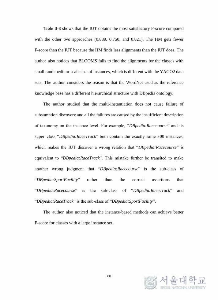
60
Table 3-3 shows that the IUT obtains the most satisfactory F-score compared
with the other two approaches (0.889, 0.750, and 0.821). The HM gets fewer
F-score than the IUT because the HM finds less alignments than the IUT does. The
author also notices that BLOOMS fails to find the alignments for the classes with
small- and medium-scale size of instances, which is different with the YAGO2 data
sets. The author considers the reason is that the WordNet used as the reference
knowledge base has a different hierarchical structure with DBpedia ontology.
The author studied that the multi-instantiation does not cause failure of
subsumption discovery and all the failures are caused by the insufficient description
of taxonomy on the instance level. For example, “DBpedia:Racecourse” and its
super class “DBpedia:RaceTrack” both contain the exactly same 300 instances,
which makes the IUT discover a wrong relation that “DBpedia:Racecourse” is
equivalent to “DBpedia:RaceTrack”. This mistake further be transited to make
another wrong judgment that “DBpedia:Racecourse” is the sub-class of
“DBpedia:SportFacility” rather than the correct assertions that
“DBpedia:Racecourse” is the sub-class of “DBpedia:RaceTrack” and
“DBpedia:RaceTrack” is the sub-class of “DBpedia:SportFacility”.
The author also noticed that the instance-based methods can achieve better
F-score for classes with a large instance set.
61
3.5.3 Inter-Subsumption and Equivalence Relations for
YAGO2-DBpedia
Figure 3-7: Running time of the three methods of YAGO2-DBpedia for inter-subsumption alignment.
The author tries to align 358 classes from YAGO2 knowledge base to 358 classes
from DBpedia ontology using subsumption relation. Same as the two previous
experiments, the author separated classes into three instance-range groups. Figure
3-7 shows that the IUT is the fastest method for aligning the classes in all the
instance-ranges.
1.0E+00
1.0E+01
1.0E+02
1.0E+03
1.0E+04
0-100 100-500 500-10000
IUT HM BLOOMS(ms)

62
Table 3-4: Results of subsumption alignment in YAGO2-DBpedia.
#instances(0-100)
Precision Recall F-score
IUT 0.0 0.0 NaN
HM NaN 0.0 NaN
BLOOMS NaN 0.0 NaN
#instances [100-500)
Precision Recall F-score
IUT 1.0 0.50 0.667
HM 0.250 0.250 0.250
BLOOMS NaN 0.0 NaN
#instances [500-10,000)
Precision Recall F-score
IUT 0.0 0.0 NaN
HM 1.0 0.40 0.571
BLOOMS 0.053 0.034 0.041
Overall (0-10,000)
Precision Recall F-score
IUT 0.301 0.546 0.388
HM 0.189 0.162 0.175
BLOOMS 0 0 NaN
63
Unlike the performance of the methods for intra-subsumptions in YAGO2 and
DBpedia, the methods perform variously shown in Table 3-4. The IUT gets the best
F-score in the overall data set (0.388), in medium-scale (0.667), and the HM gets the
best F-score in large-scale (0.571). The reasons that cause the failures of the IUT to
find the inter-subsumption relations are different with the reasons for
intra-subsumption relations discovery. Different taxonomic systems are designed
for different purposes, which make the scope of the class definitions different and
distinctly instantiate the classes. Therefore, the classes having equivalence relation
may not strictly satisfy the Definition 3-1 on the instance-level. More specifically,
(1) two classes without subsumption relation from different ontologies share all
instances from the class with a smaller cardinality, which is known as a false
positive. For example, “YAGO:Ballplayer109835506” has 20,299 instances that are
all included by “DBpedia:Person”. However, “YAGO:Ballplayer109835506” and
“DBpedia:Person” are not connected by subsumption relation. (2) two classes with
subsumption relation from different ontologies share the common instances that are
only part of each instance set from the classes, which is known as a false negative.
For example, “DBpediaOntology:SpaceMission” contains five instances (“Ares
I-X”, “Ares V-X”, “Apollo–Soyuz Test Project”, “Ares I-Y”, “Hypersonic Flight
Experiment”) and only the first four instances are contained by
“YAGO:Mission108403225”, which makes the instance-based methods fail to
establish a subsumption relation. The taxonomic system in YAGO2 has more
appropriate classes (“YAGO:Spaceflight100313502”, “YAGO:Travel100295701”,
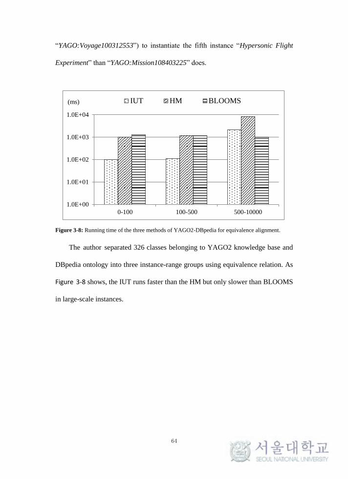
64
“YAGO:Voyage100312553”) to instantiate the fifth instance “Hypersonic Flight
Experiment” than “YAGO:Mission108403225” does.
Figure 3-8: Running time of the three methods of YAGO2-DBpedia for equivalence alignment.
The author separated 326 classes belonging to YAGO2 knowledge base and
DBpedia ontology into three instance-range groups using equivalence relation. As
Figure 3-8 shows, the IUT runs faster than the HM but only slower than BLOOMS
in large-scale instances.
1.0E+00
1.0E+01
1.0E+02
1.0E+03
1.0E+04
0-100 100-500 500-10000
IUT HM BLOOMS(ms)

65
Table 3-5: Results of equivalence alignment in YAGO2-DBpedia.
#instances(0-100)
Precision Recall F-score
IUT 1.0 0.20 0.333
HM 1.0 0.267 0.421
BLOOMS 1.0 0.067 0.125
#instances [100-500)
Precision Recall F-score
IUT 1.0 0.417 0.588
HM 1.0 0.417 0.588
BLOOMS 0.773 0.708 0.739
#instances [500-10,000)
Precision Recall F-score
IUT 0.953 0.621 0.753
HM 1.0 0.273 0.429
BLOOMS 0.739 0.773 0.756
Overall (0-10,000)
Precision Recall F-score
IUT 0.865 0.509 0.641
HM 0.935 0.264 0.411
BLOOMS 0.552 0.656 0.600
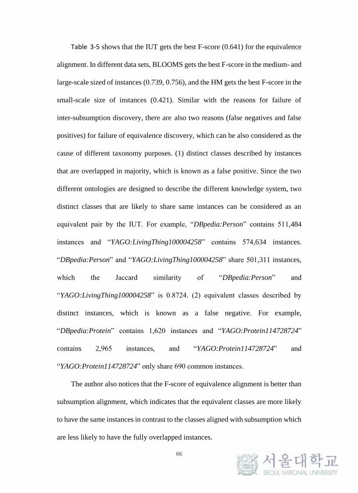
66
Table 3-5 shows that the IUT gets the best F-score (0.641) for the equivalence
alignment. In different data sets, BLOOMS gets the best F-score in the medium- and
large-scale sized of instances (0.739, 0.756), and the HM gets the best F-score in the
small-scale size of instances (0.421). Similar with the reasons for failure of
inter-subsumption discovery, there are also two reasons (false negatives and false
positives) for failure of equivalence discovery, which can be also considered as the
cause of different taxonomy purposes. (1) distinct classes described by instances
that are overlapped in majority, which is known as a false positive. Since the two
different ontologies are designed to describe the different knowledge system, two
distinct classes that are likely to share same instances can be considered as an
equivalent pair by the IUT. For example, “DBpedia:Person” contains 511,484
instances and “YAGO:LivingThing100004258” contains 574,634 instances.
“DBpedia:Person” and “YAGO:LivingThing100004258” share 501,311 instances,
which the Jaccard similarity of “DBpedia:Person” and
“YAGO:LivingThing100004258” is 0.8724. (2) equivalent classes described by
distinct instances, which is known as a false negative. For example,
“DBpedia:Protein” contains 1,620 instances and “YAGO:Protein114728724”
contains 2,965 instances, and “YAGO:Protein114728724” and
“YAGO:Protein114728724” only share 690 common instances.
The author also notices that the F-score of equivalence alignment is better than
subsumption alignment, which indicates that the equivalent classes are more likely
to have the same instances in contrast to the classes aligned with subsumption which
are less likely to have the fully overlapped instances.
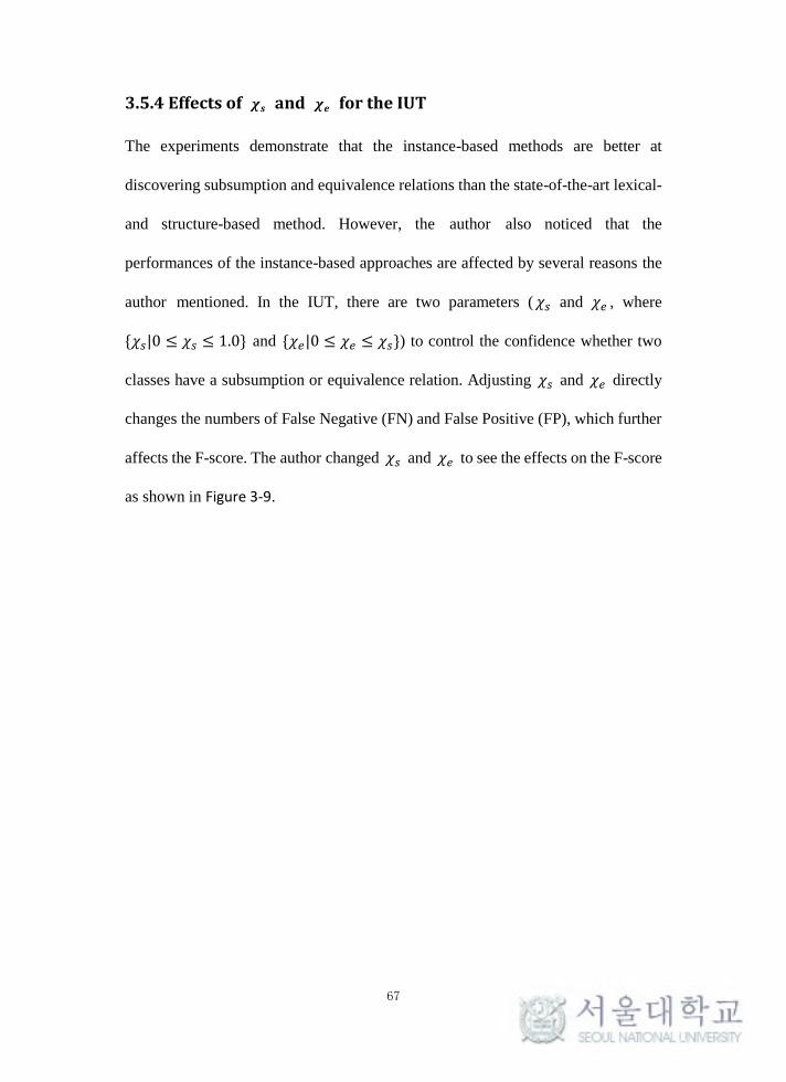
67
3.5.4 Effects of 𝝌𝒔 and 𝝌𝒆 for the IUT
The experiments demonstrate that the instance-based methods are better at
discovering subsumption and equivalence relations than the state-of-the-art lexical-
and structure-based method. However, the author also noticed that the
performances of the instance-based approaches are affected by several reasons the
author mentioned. In the IUT, there are two parameters (𝜒𝑠 and 𝜒𝑒 , where
{𝜒𝑠|0 ≤ 𝜒𝑠 ≤ 1.0} and {𝜒𝑒|0 ≤ 𝜒𝑒 ≤ 𝜒𝑠}) to control the confidence whether two
classes have a subsumption or equivalence relation. Adjusting 𝜒𝑠 and 𝜒𝑒 directly
changes the numbers of False Negative (FN) and False Positive (FP), which further
affects the F-score. The author changed 𝜒𝑠 and 𝜒𝑒 to see the effects on the F-score
as shown in Figure 3-9.
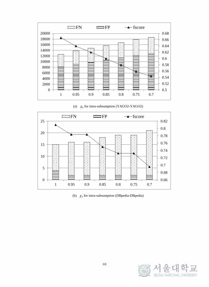
68
(a) 𝜒𝑠 for intra-subsumption (YAGO2-YAGO2)
(b) 𝜒𝑠 for intra-subsumption (DBpedia-DBpedia)
0.5
0.52
0.54
0.56
0.58
0.6
0.62
0.64
0.66
0.68
0
2000
4000
6000
8000
10000
12000
14000
16000
18000
20000
1 0.95 0.9 0.85 0.8 0.75 0.7
FN FP fscore
0.66
0.68
0.7
0.72
0.74
0.76
0.78
0.8
0.82
0
5
10
15
20
25
1 0.95 0.9 0.85 0.8 0.75 0.7
FN FP fscore
69
(c) 𝜒𝑠 for inter-subsumption (YAGO2-DBpedia)
(d) 𝜒𝑒 for inter-equivalence (YAGO2-DBpedia)
Figure 3-9: 𝜒𝑠 and 𝜒𝑒 for the IUT.
As Figure 3-9 (a, b, and c) show, decreasing 𝜒𝑠 hurts the F-score as the
number of FN and FP increases. The main reason for failures of inter-subsumption
discovery is FP that increases along with the decrease of 𝜒𝑠. The lower 𝜒𝑠 allows
more candidate pairs to be considered as positives, which increases the recall but
decreases the precision. Different with inter-subsumption discovery, FN is the main
0.36
0.365
0.37
0.375
0.38
0.385
0.39
0
100
200
300
400
500
600
700
800
1 0.95 0.9 0.85 0.8 0.75 0.7
FN FP fscore
0.3
0.35
0.4
0.45
0.5
0.55
0.6
0.65
0.7
0.75
0.8
0
50
100
150
200
250
300
350
400
0.05 0.1 0.15 0.2 0.25 0.3 0.35 0.4 0.45 0.5 0.55 0.6 0.65 0.7 0.75 0.8 0.85 0.9
FN FP fscore
70
reason for failures of intra-subsumption discovery in DBpedia-DBpedia, which
increases along with the decreases of 𝜒𝑠 . The insufficient description of the
intra-taxonomy on the instance level is the main reason of alignment failures for
DBpedia ontology, lowering 𝜒𝑠 allows more classes to establish subsumption
relations, which amplifies the errors caused by the effects of insufficient taxonomic
description on the instance level. The amplification decreases the recall and further
decreases the F-score. The intra-subsumption in YAGO2-YAGO2 is affected by
two reasons (insufficient taxonomic description on the instance level and
multi-instantiation). Lowering the threshold of subsumption establishing, which is
caused by decreasing of 𝜒𝑠, amplifies both FN and FP hence decreases the recall
and the precision.
Figure 3-9 (d) shows that 𝜒𝑒 gets the best F-score when 𝜒𝑒 = 0.25. The
author observes that increasing 𝜒𝑒 boosts the F-score before the F-score reaching
the summit, and hurts the F-score after overpassing the summit. Before 𝜒𝑒 arriving
0.25, increases of 𝜒𝑒 raises threshold that traps more non-equivalent classes, which
decrease FN and FP. Along with 𝜒𝑒 increases and overpasses 0.25, fewer candidate
pairs are considered to be equivalent, which increases FN and FP.
From the Figure 3-9, the author gets two important hints for setting 𝜒𝑠 and 𝜒𝑒
where {𝜒𝑠|0 ≤ 𝜒𝑠 ≤ 1.0} and {𝜒𝑒|0 ≤ 𝜒𝑒 ≤ 𝜒𝑠} , that is, the higher 𝜒𝑠 is the
better it is for subsumption discovery, and the lower 𝜒𝑒 is the better it is for
equivalence discovery before 𝜒𝑒 = 0.25.
71
3.6 Discussions
The IUT is an instance-based schema alignment algorithm, which heavily depends
on the description of ontology on the instance level. The results of the alignment of
the IUT can be affected by two reasons as the author discussed in Section 3.5,
which are insufficient taxonomic description on the instance level and
multi-instantiation. The motley instantiation strategies for diversity ontologies
weaken the subsumption and equivalence detections.
Another problem what instance-based methods should care is the issue caused
by the asymmetric ontology update. The alignment of two classes from two
ontologies changes if the updating speeds of two ontologies are different. For
example, updating DBpedia 3.9 that uses the Wikipedia data in April 2013 from
DBpedia 3.8 that uses the Wikipedia data in June 2012 costs nine months, but
updating YAGO2 2.5 that uses the Wikipedia data in December 2012 from YAGO2
2.4 that uses the Wikipedia data in August 2010 costs more than two years. The
imbalanced updating speed can change the original alignment results. For instance,
the “DBpedia: Artery” in DBpedia 3.9 contains all the instances in
“YAGO:Artery105333777” in YAGO2 2.4, which the IUT considers a subsumption
relation between the two classes. However, the “DBpedia:Artery” in DBpedia 3.9
shares part of all instances (303) in “YAGO:Artery105333777” in YAGO2 2.5,
which increase the Jaccard similarity into 0.75 and defines the relation as
equivalence. In this study, the author simply removes the instances only used in one
data resource to reduce the effects of the asymmetric ontology update. However, the
added or deleted instances in an updated version can more precisely describe a class
72
and correct some errors in the alignments for the previous version that is poorly
designed. A comprehensive solution is a new research direction for the future work.
There are two assumptions for instance-based methods: (1) instance-level
alignment is established. (2) ontology has a hierarchical structure on the
schema-level. Linked Data creates links to connect data in different sources based
on the Web (Bizer et al., 2009). Therefore, links are one of the most important
factors to evaluate the quality of a linked data set. Most famous linked data sets
already have abundant links. For example, DBpedia has 39,012,034 links connected
with a variety of databases, including BBC music, DailyMed, New York Times, etc.
For those are not connected with other linked data sets, one solution is to establish
instance alignments with existing instance alignment algorithms, which is proposed
by PARIS (Suchanek et al., 2011), and use existing link discovery frameworks, such
as Silk (Volz, Bizer, Gaedke, & Kobilarov, 2009). For the second assumption, some
ontologies in LOD lack the hierarchical structure, which will fail the proposed
approach. One solution is to build taxonomy automatically with the help of
probability models, logic rules or thesauri (Bedini & Nguyen, 2007). The author has
proposed a solution in Chapter 5 that introduces the methods to automatically
generate hierarchical schema structure for Linked Data in detail.
In the proposed method, only inter-linked instances are used. There raises a
discussion on the meaning of using of inter-linked instances in our data
pre-processing.
In Semantic Web, an ontology is constructed based on Open-World
Assumption (OWA), which admits incompleteness of instances at a given time.
73
This incompleteness in describing a concept is due to many reasons, such as
unintentional omission of instances though they are exposed to the ontology
developer, and lack of awareness of the existence of instances that deem the status
of being included in the concept. Therefore, even for the same concept, two
ontologies may have different instance sets attached to the concept, since the
different instance spaces are deemed as legitimate within their sphere of known
explored world.
In concept comparison, the incompleteness of concept extensions (i.e.,
instances) weakens the usefulness of instances as the description of understanding,
or definition, of concepts, because the incompleteness itself may be the cause of
varying instantiations of the concepts. In short, the instances the author gathered are
just one possible representation of a concept - there may be many more such cases.
In order to come up with a way that produces a convincing measure for similarity
between concepts, one has to rely on truth, which in this study is links. Links are
created externally, and the author has no control over, or rather should not have
control over. Hence, links are taken as the sole truth statements that prove the
legitimacy of similarity between two concepts. As for unlinked instances, the author
takes them as neither untrue nor true, since it is beyond the scope of this study. In
case a new link is created in the future between two instances which did not have a
link between them, the author's method will take it as a new truth statement and
proceeds as it is designed to.
Therefore, unlinked instances are removed, and the remaining instances are
conflated into one instance space. For example, to align two different versions of

74
DBpedia Ontology, DBpedia 3.9 and DBpedia 2014, removing the instances only
existing in DBpedia 2014 can eliminate the mismatched concepts because of the
new added instances (from April 2013 to May 2014) that are not acknowledged by
DBpedia 3.9.
75
3.7 Conclusion
In this chapter, the author proposed the IUT that is an instance-based schema
alignment algorithm. The IUT builds a unified taxonomy for all the classes from
two ontologies to obtain the alignments. The position of each class is decided by the
common instances shared with other classes in the unified taxonomy. The author
tested the IUT with DBpedia and YAGO2, and compared the IUT with two
state-of-the-art methods for schema alignments in LOD. The experiments show the
IUT outperforms the methods in F-score. The experiments also illustrate that
ontology with a larger number of instances is more likely to have a good F-score of
the IUT. The author also observed the reasons of aligning failures for the IUT, that
is, insufficient taxonomic description on the instance level and multi-instantiation in
the intra-subsumption alignment, and different taxonomic structure of ontologies
for diversity purposes in the inter-subsumption and equivalence alignment. Two
parameters for the IUT are tested to control the alignment failures. The author
discussed limitations of proposed method and gives several solutions to improve the
works.
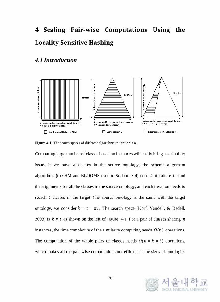
76
4 Scaling Pair-wise Computations Using the
Locality Sensitive Hashing
4.1 Introduction
Figure 4-1: The search spaces of different algorithms in Section 3.4.
Comparing large number of classes based on instances will easily bring a scalability
issue. If we have 𝑘 classes in the source ontology, the schema alignment
algorithms (the HM and BLOOMS used in Section 3.4) need 𝑘 iterations to find
the alignments for all the classes in the source ontology, and each iteration needs to
search 𝑡 classes in the target (the source ontology is the same with the target
ontology, we consider 𝑘 = 𝑡 = 𝑚). The search space (Korf, Yandell, & Bedell,
2003) is 𝑘 × 𝑡 as shown on the left of Figure 4-1. For a pair of classes sharing 𝑛
instances, the time complexity of the similarity computing needs 𝑂(𝑛) operations.
The computation of the whole pairs of classes needs 𝑂(𝑛 × 𝑘 × 𝑡) operations,
which makes all the pair-wise computations not efficient if the sizes of ontologies
77
are too large. The IUT decreases the search space with the unified graph (the search
space at the center of Figure 4-1) but could still meet a scalability issue.
The Locality Sensitive Hashing (LSH) (Rajaraman & Ullman, 2011) is a
probabilistic dimension reduction algorithm. The basic idea of LSH is to map sets of
values into hash values with reduced dimensions, and put similar sets into buckets
with a high probability. LSH can be used to reduce large pair-wise computations,
and is further adapted in instance-based schema mapping (Duan et al., 2012). The
author adapts the basic idea of the LSH that uses MinHash to estimate the
probability of subsumption (Definition 3-1) and equivalence (Definitions 3-2 and
3-3) in Section 3.3.3 to decrease the time complexity of a similarity computation,
and use bandings to reduce the search space (on the right of Figure 4-1) used in
Algorithm 3-1. The author performs an experiment of scaling the IUT based on LSH
for YAGO2-YAGO2 intra-subsumption alignment task performed in Section 3.5.1.
The experiment demonstrates that the running time of the original IUT can be
reduced by 94% with a 5% loss in F-score using the proposed scaling method.
The content of this chapter is mainly based on the author’s previous work
published (Zong et al., 2015). The rest of this chapter is organized as follows:
Section 4.2 introduces MinHash and banding method of the LSH, and details on the
IUT(M), an IUT-based schema algorithm with the LSH; Section 4.3 introduces the
scaling results of the IUT(M) for YAGO2-YAGO2 intra-subsumption alignment
task. Section 4.4 discusses limitations of this chapter, and Section 4.5 concludes this
study.
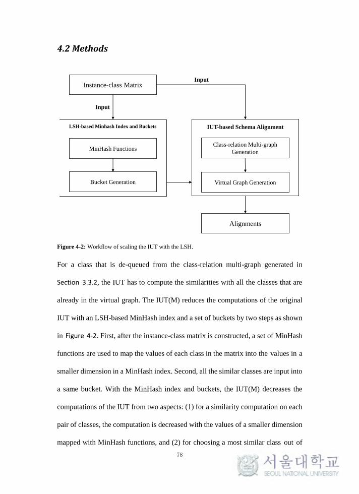
78
4.2 Methods
Figure 4-2: Workflow of scaling the IUT with the LSH.
For a class that is de-queued from the class-relation multi-graph generated in
Section 3.3.2, the IUT has to compute the similarities with all the classes that are
already in the virtual graph. The IUT(M) reduces the computations of the original
IUT with an LSH-based MinHash index and a set of buckets by two steps as shown
in Figure 4-2. First, after the instance-class matrix is constructed, a set of MinHash
functions are used to map the values of each class in the matrix into the values in a
smaller dimension in a MinHash index. Second, all the similar classes are input into
a same bucket. With the MinHash index and buckets, the IUT(M) decreases the
computations of the IUT from two aspects: (1) for a similarity computation on each
pair of classes, the computation is decreased with the values of a smaller dimension
mapped with MinHash functions, and (2) for choosing a most similar class out of
Instance-class Matrix
MinHash Functions
Bucket Generation
Class-relation Multi-graph
Generation
Input
Virtual Graph Generation
Alignments
LSH-based Minhash Index and Buckets
Input
IUT-based Schema Alignment
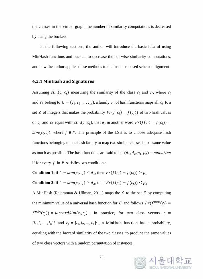
79
the classes in the virtual graph, the number of similarity computations is decreased
by using the buckets.
In the following sections, the author will introduce the basic idea of using
MinHash functions and buckets to decrease the pairwise similarity computations,
and how the author applies these methods to the instance-based schema alignment.
4.2.1 MinHash and Signatures
Assuming 𝑠𝑖𝑚(𝑐𝑖 , 𝑐𝑗) measuring the similarity of the class 𝑐𝑖 and 𝑐𝑗 , where 𝑐𝑖
and 𝑐𝑗 belong to 𝐶 = {𝑐1, 𝑐2, … , 𝑐𝑚}, a family 𝐹 of hash functions maps all 𝑐𝑖 to a
set 𝑍 of integers that makes the probability 𝑃𝑟(𝑓(𝑐𝑖) = 𝑓(𝑐𝑗)) of two hash values
of 𝑐𝑖 and 𝑐𝑗 equal with 𝑠𝑖𝑚(𝑐𝑖 , 𝑐𝑗), that is, in another word 𝑃𝑟(𝑓(𝑐𝑖) = 𝑓(𝑐𝑗)) =
𝑠𝑖𝑚(𝑐𝑖, 𝑐𝑗), where 𝑓 ∈ 𝐹. The principle of the LSH is to choose adequate hash
functions belonging to one hash family to map two similar classes into a same value
as much as possible. The hash functions are said to be (𝑑1, 𝑑2, 𝑝1, 𝑝2) − 𝑠𝑒𝑛𝑠𝑖𝑡𝑖𝑣𝑒
if for every 𝑓 in 𝐹 satisfies two conditions:
Condition 1: if 1 − 𝑠𝑖𝑚(𝑐𝑖, 𝑐𝑗) ≤ 𝑑1, then 𝑃𝑟(𝑓(𝑐𝑖) = 𝑓(𝑐𝑗)) ≥ 𝑝1
Condition 2: if 1 − 𝑠𝑖𝑚(𝑐𝑖, 𝑐𝑗) ≥ 𝑑2, then 𝑃𝑟(𝑓(𝑐𝑖) = 𝑓(𝑐𝑗)) ≤ 𝑝2
A MinHash (Rajaraman & Ullman, 2011) maps the 𝐶 to the set 𝑍 by computing
the minimum value of a universal hash function for 𝐶 and follows 𝑃𝑟(𝑓𝑚𝑖𝑛(𝑐𝑖) =
𝑓𝑚𝑖𝑛(𝑐𝑗)) = 𝑗𝑎𝑐𝑐𝑎𝑟𝑑𝑆𝑖𝑚(𝑐𝑖, 𝑐𝑗) . In practice, for two class vectors 𝑐𝑖 =
[𝑖1, 𝑖2, … , 𝑖𝑛]𝑇 and 𝑐𝑗 = [𝑖1, 𝑖2, … , 𝑖𝑛]
𝑇 , a MinHash function has a probability,
equaling with the Jaccard similarity of the two classes, to produce the same values
of two class vectors with a random permutation of instances.
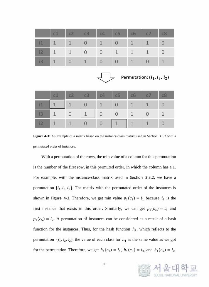
80
Figure 4-3: An example of a matrix based on the instance-class matrix used in Section 3.3.2 with a
permutated order of instances.
With a permutation of the rows, the min value of a column for this permutation
is the number of the first row, in this permuted order, in which the column has a 1.
For example, with the instance-class matrix used in Section 3.3.2, we have a
permutation {𝑖1, 𝑖3, 𝑖2}. The matrix with the permutated order of the instances is
shown in Figure 4-3. Therefore, we get min value 𝑝1(𝑐1) = 𝑖1 because 𝑖1 is the
first instance that exists in this order. Similarly, we can get 𝑝1(𝑐3) = 𝑖3 and
𝑝1(𝑐5) = 𝑖2. A permutation of instances can be considered as a result of a hash
function for the instances. Thus, for the hash function ℎ1, which reflects to the
permutation {𝑖1, 𝑖3, 𝑖2}, the value of each class for ℎ1 is the same value as we got
for the permutation. Therefore, we get ℎ1(𝑐1) = 𝑖1, ℎ1(𝑐3) = 𝑖3, and ℎ1(𝑐5) = 𝑖2.
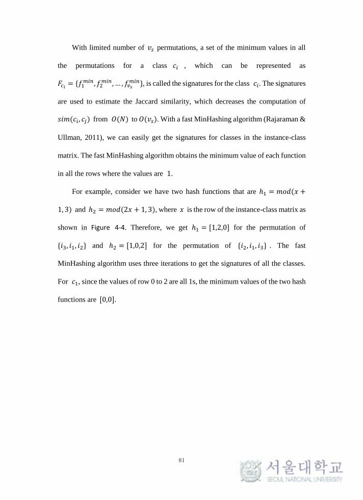
81
With limited number of 𝑣𝑠 permutations, a set of the minimum values in all
the permutations for a class 𝑐𝑖 , which can be represented as
𝐹𝑐𝑖 = {𝑓1𝑚𝑖𝑛, 𝑓2
𝑚𝑖𝑛, … , 𝑓𝑣𝑠𝑚𝑖𝑛}, is called the signatures for the class 𝑐𝑖. The signatures
are used to estimate the Jaccard similarity, which decreases the computation of
𝑠𝑖𝑚(𝑐𝑖, 𝑐𝑗) from 𝑂(𝑁) to 𝑂(𝑣𝑠). With a fast MinHashing algorithm (Rajaraman &
Ullman, 2011), we can easily get the signatures for classes in the instance-class
matrix. The fast MinHashing algorithm obtains the minimum value of each function
in all the rows where the values are 1.
For example, consider we have two hash functions that are ℎ1 = 𝑚𝑜𝑑(𝑥 +
1, 3) and ℎ2 = 𝑚𝑜𝑑(2𝑥 + 1, 3), where 𝑥 is the row of the instance-class matrix as
shown in Figure 4-4. Therefore, we get ℎ1 = [1,2,0] for the permutation of
{𝑖3, 𝑖1, 𝑖2} and ℎ2 = [1,0,2] for the permutation of {𝑖2, 𝑖1, 𝑖3} . The fast
MinHashing algorithm uses three iterations to get the signatures of all the classes.
For 𝑐1, since the values of row 0 to 2 are all 1s, the minimum values of the two hash
functions are [0,0].
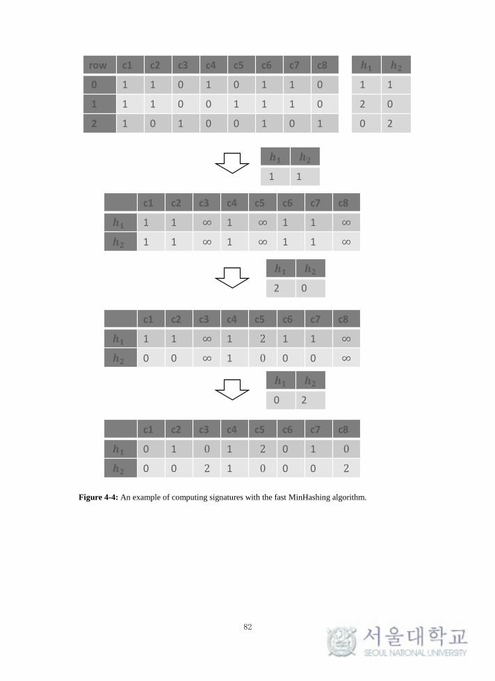
82
Figure 4-4: An example of computing signatures with the fast MinHashing algorithm.
row c1 c2 c3 c4 c5 c6 c7 c8
0 1 1 0 1 0 1 1 0
1 1 1 0 0 1 1 1 0
2 1 0 1 0 0 1 0 1
1 1
2 0
0 2
c1 c2 c3 c4 c5 c6 c7 c8
1 1 1 1 1
1 1 1 1 1
1 1
c1 c2 c3 c4 c5 c6 c7 c8
1 1 1 2 1 1
0 0 1 0 0 0
2 0
c1 c2 c3 c4 c5 c6 c7 c8
0 1 0 1 2 0 1 0
0 0 2 1 0 0 0 2
0 2
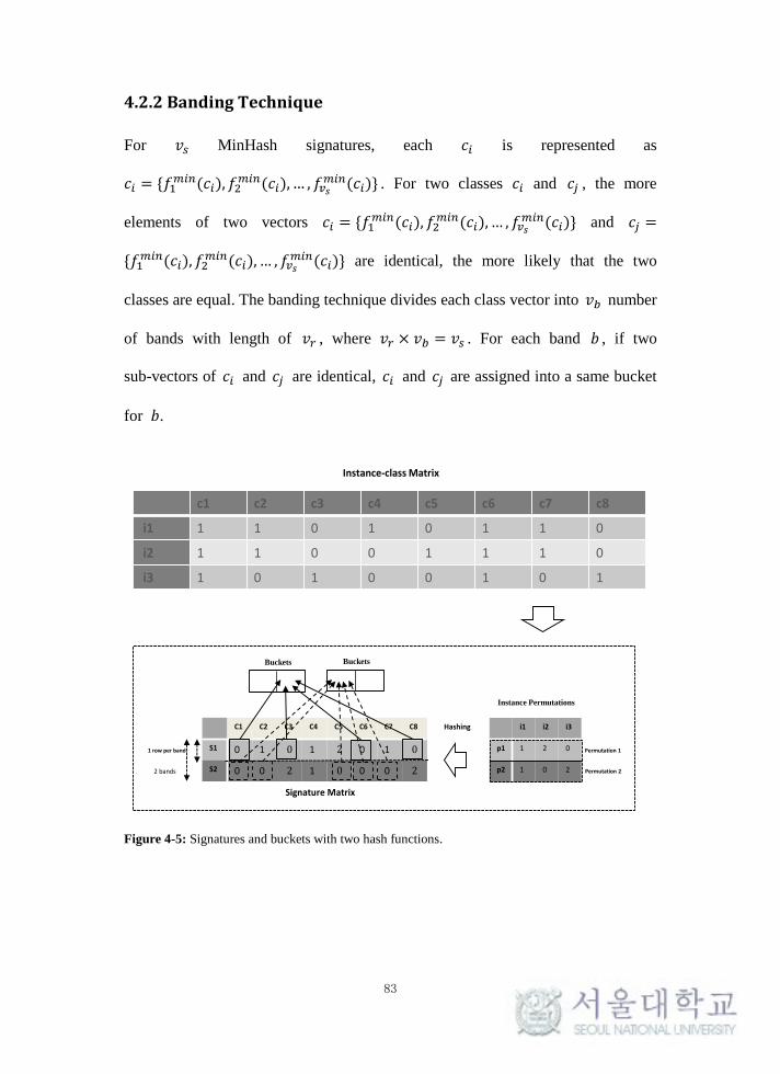
83
4.2.2 Banding Technique
For 𝑣𝑠 MinHash signatures, each 𝑐𝑖 is represented as
𝑐𝑖 = {𝑓1𝑚𝑖𝑛(𝑐𝑖), 𝑓2
𝑚𝑖𝑛(𝑐𝑖),… , 𝑓𝑣𝑠𝑚𝑖𝑛(𝑐𝑖)} . For two classes 𝑐𝑖 and 𝑐𝑗 , the more
elements of two vectors 𝑐𝑖 = {𝑓1𝑚𝑖𝑛(𝑐𝑖), 𝑓2
𝑚𝑖𝑛(𝑐𝑖),… , 𝑓𝑣𝑠𝑚𝑖𝑛(𝑐𝑖)} and 𝑐𝑗 =
{𝑓1𝑚𝑖𝑛(𝑐𝑖), 𝑓2
𝑚𝑖𝑛(𝑐𝑖),… , 𝑓𝑣𝑠𝑚𝑖𝑛(𝑐𝑖)} are identical, the more likely that the two
classes are equal. The banding technique divides each class vector into 𝑣𝑏 number
of bands with length of 𝑣𝑟 , where 𝑣𝑟 × 𝑣𝑏 = 𝑣𝑠 . For each band 𝑏 , if two
sub-vectors of 𝑐𝑖 and 𝑐𝑗 are identical, 𝑐𝑖 and 𝑐𝑗 are assigned into a same bucket
for 𝑏.
Figure 4-5: Signatures and buckets with two hash functions.
C1 C2 C3 C4 C5 C6 C7 C8
S1 0 1 0 1 2 0 1 0
S2 0 0 2 1 0 0 0 2
i1 i2 i3
p1 1 2 0
p2 1 0 2
Signature Matrix
Instance Permutations
1 row per band
2 bands
Hashing
Permutation 1
Permutation 2
c1 c2 c3 c4 c5 c6 c7 c8
i1 1 1 0 1 0 1 1 0
i2 1 1 0 0 1 1 1 0
i3 1 0 1 0 0 1 0 1
Instance-class Matrix
Buckets Buckets
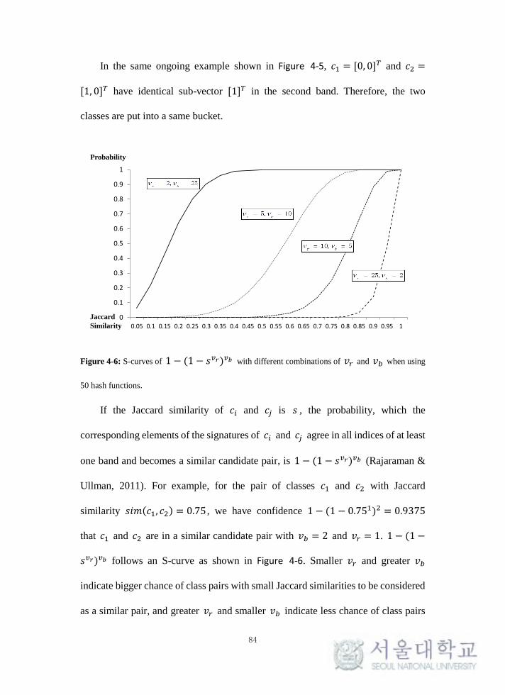
84
In the same ongoing example shown in Figure 4-5, 𝑐1 = [0, 0]𝑇 and 𝑐2 =
[1, 0]𝑇 have identical sub-vector [1]𝑇 in the second band. Therefore, the two
classes are put into a same bucket.
Figure 4-6: S-curves of 1 − (1 − 𝑠𝑣𝑟)𝑣𝑏 with different combinations of 𝑣𝑟 and 𝑣𝑏 when using
50 hash functions.
If the Jaccard similarity of 𝑐𝑖 and 𝑐𝑗 is 𝑠 , the probability, which the
corresponding elements of the signatures of 𝑐𝑖 and 𝑐𝑗 agree in all indices of at least
one band and becomes a similar candidate pair, is 1 − (1 − 𝑠𝑣𝑟)𝑣𝑏 (Rajaraman &
Ullman, 2011). For example, for the pair of classes 𝑐1 and 𝑐2 with Jaccard
similarity 𝑠𝑖𝑚(𝑐1, 𝑐2) = 0.75 , we have confidence 1 − (1 − 0.751)2 = 0.9375
that 𝑐1 and 𝑐2 are in a similar candidate pair with 𝑣𝑏 = 2 and 𝑣𝑟 = 1. 1 − (1 −
𝑠𝑣𝑟)𝑣𝑏 follows an S-curve as shown in Figure 4-6. Smaller 𝑣𝑟 and greater 𝑣𝑏
indicate bigger chance of class pairs with small Jaccard similarities to be considered
as a similar pair, and greater 𝑣𝑟 and smaller 𝑣𝑏 indicate less chance of class pairs
0
0.1
0.2
0.3
0.4
0.5
0.6
0.7
0.8
0.9
1
0.05 0.1 0.15 0.2 0.25 0.3 0.35 0.4 0.45 0.5 0.55 0.6 0.65 0.7 0.75 0.8 0.85 0.9 0.95 1
Jaccard
Similarity
Probability
85
with large Jaccard similarities to be considered as a similar pair. With good tuning
of the two parameters, the computations of choosing the most similar class in a
virtual graph for a de-queued class from the class-relation multi-graph can be
dramatically decreased.
4.2.3 Scaling the IUT with MinHash and Banding
The author scales the IUT with MinHash and banding techniques that are used to
reduce the pair-wise similar computation of Jaccard similarity, and the author calls
it IUT(M). The IUT(M) builds 𝑣𝑠 MinHash functions and bands the signature
matrix with 𝑣𝑟 rows and 𝑣𝑠
𝑣𝑟 bands (line 2 in Algorithm 4-1). The similar candidate
pairs are used to restrict the search space for discovering a relation for a class in the
graph (line 7 in Algorithm 4-1). In practice, the IUT(M) discards the multi-graph
that is used to sort the important classes and simply sorts classes by the number of
instances (line 3 in Algorithm 4-1).
In order to accommodate the subsumption relation discovering using Equation
3-1, the IUT(M) computes the 𝑠𝑖𝑚′(𝑐𝑖, 𝑐𝑗) with existing estimated Jaccard
similarity 𝑗𝑎𝑐𝑐𝑎𝑟𝑑′(𝑐𝑖, 𝑐𝑗) by MinHash as follows:
𝑠𝑢𝑏′(𝑐𝑖, 𝑐𝑗) =𝑗𝑎𝑐𝑐𝑎𝑟𝑑′(𝑐𝑖,𝑐𝑗)
𝑗𝑎𝑐𝑐𝑎𝑟𝑑′(𝑐𝑖,𝑐𝑗)+1× (1 +
|𝑐𝑗|
|𝑐𝑖|) (4.1)
. The processing of the IUT(M) is shown in Algorithm 4-1.
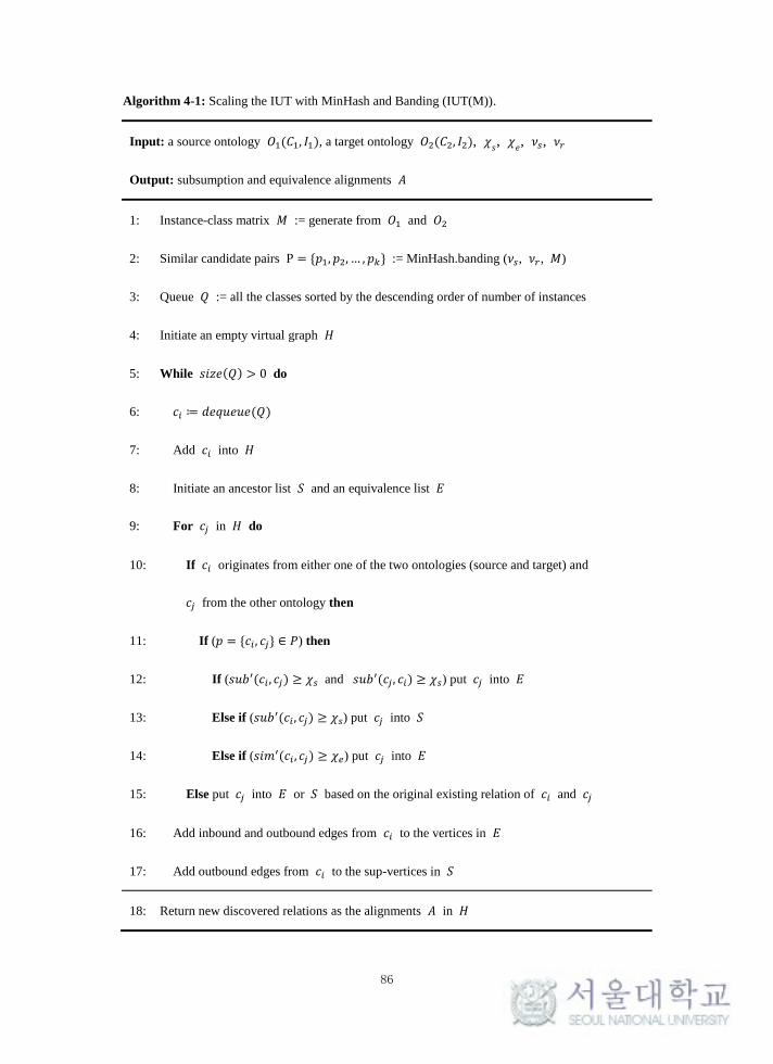
86
Algorithm 4-1: Scaling the IUT with MinHash and Banding (IUT(M)).
Input: a source ontology 𝑂1(𝐶1, 𝐼1), a target ontology 𝑂2(𝐶2, 𝐼2), 𝜒𝑠, 𝜒𝑒, 𝜈𝑠, 𝜈𝑟
Output: subsumption and equivalence alignments 𝐴
1: Instance-class matrix 𝑀 := generate from 𝑂1 and 𝑂2
2: Similar candidate pairs P = {𝑝1, 𝑝2, … , 𝑝𝑘} := MinHash.banding (𝜈𝑠, 𝜈𝑟, 𝑀)
3: Queue 𝑄 := all the classes sorted by the descending order of number of instances
4: Initiate an empty virtual graph 𝐻
5: While 𝑠𝑖𝑧𝑒(𝑄) > 0 do
6: 𝑐𝑖 ≔ 𝑑𝑒𝑞𝑢𝑒𝑢𝑒(𝑄)
7: Add 𝑐𝑖 into 𝐻
8: Initiate an ancestor list 𝑆 and an equivalence list 𝐸
9: For 𝑐𝑗 in 𝐻 do
10: If 𝑐𝑖 originates from either one of the two ontologies (source and target) and
𝑐𝑗 from the other ontology then
11: If (𝑝 = {𝑐𝑖 , 𝑐𝑗} ∈ 𝑃) then
12: If (𝑠𝑢𝑏′(𝑐𝑖 , 𝑐𝑗) ≥ 𝜒𝑠 and 𝑠𝑢𝑏′(𝑐𝑗 , 𝑐𝑖) ≥ 𝜒𝑠) put 𝑐𝑗 into 𝐸
13: Else if (𝑠𝑢𝑏′(𝑐𝑖 , 𝑐𝑗) ≥ 𝜒𝑠) put 𝑐𝑗 into 𝑆
14: Else if (𝑠𝑖𝑚′(𝑐𝑖 , 𝑐𝑗) ≥ 𝜒𝑒) put 𝑐𝑗 into 𝐸
15: Else put 𝑐𝑗 into 𝐸 or 𝑆 based on the original existing relation of 𝑐𝑖 and 𝑐𝑗
16: Add inbound and outbound edges from 𝑐𝑖 to the vertices in 𝐸
17: Add outbound edges from 𝑐𝑖 to the sup-vertices in 𝑆
18: Return new discovered relations as the alignments 𝐴 in 𝐻
87
4.3 Experiment
As Section 3.5.1 shows, big size data (YAGO2-YAGO2) addresses the scalability
problem in schema alignment. The author scales the IUT by using the LSH and
MinHash function. The banding technology makes the possibility of a similar
candidate pair follow 1 − (1 − 𝑠𝜈𝑟)𝜈𝑠𝜈𝑟 . Adjusting
𝜈𝑠
𝜈𝑟 can change the number of
candidate pairs to be compared. For example, if 𝜈𝑠 = 1,000, decreasing 𝜈𝑟 from
“10” to “5” makes the possibility, which one pair with similarity “0.6” to be
considered as a candidate pair, increase from 0.455 to 0.999.
The author tested the scaling algorithm the IUT(M) and compared it with the
baseline (the IUT) for YAGO2-YAGO2 that needs to be scaled (3,981,676 ms ).
Table 4-1: Efficiency of scaling the IUT for alignment in YAGO2-YAGO2 (𝜈𝑠 = 1,000).
𝝂𝒓 Time (ms)
𝑇𝐼𝑈𝑇(𝑀) 𝑇𝐼𝑈𝑇(𝑀)
𝑇𝐵
50 245,233 0.06159
20 231,484 0.058137
10 228,938 0.057498
5 226,824 0.056967
3 228,099 0.057287
2 232,039 0.058277
Baseline(B) 3,981,676
88
Table 4-2: Precision of scaling the IUT for alignment in YAGO2-YAGO2 (𝜈𝑠 = 10,00).
𝝂𝒓 Precision
𝑃𝐼𝑈𝑇(𝑀) 𝑃𝐼𝑈𝑇(𝑀) − 𝑃𝐵
50 0.809322 +0.203712
20 0.778471 +0.172861
10 0.752852 +0.147242
5 0.704648 +0.099038
3 0.690829 +0.085219
2 0.681948 +0.076338
Baseline(B) 0.60561
Table 4-3: Recall of scaling the IUT for alignment in YAGO2-YAGO2 (𝜈𝑠 = 1,000).
𝝂𝒓 Recall
𝑅𝐼𝑈𝑇(𝑀) 𝑅𝐼𝑈𝑇(𝑀) − 𝑅𝐵
50 0.022538 -0.71756
20 0.058883 -0.68122
10 0.116821 -0.62328
5 0.229866 -0.51024
3 0.398667 -0.34144
2 0.563455 -0.17665
Baseline(B) 0.740103
89
Table 4-4: F-score of scaling the IUT for alignment in YAGO2-YAGO2 (𝜈𝑠 = 1,000).
𝝂𝒓 F-score
𝐹𝐼𝑈𝑇(𝑀) 𝐹𝐼𝑈𝑇(𝑀) − 𝐹𝐵
20 0.043855 -0.62228
10 0.109484 -0.55665
5 0.202258 -0.46388
3 0.34665 -0.31949
2 0.505574 -0.16056
50 0.617065 -0.04907
Baseline(B) 0.666136
Table 4-1 to Table 4-4 show that the scaling algorithm (the IUT(M))
dramatically decreases the running time (𝑀𝑒𝑎𝑛𝑇𝐼𝑈𝑇(𝑀)
𝑇𝐵
= 0.058293) and keeps a
good F-score (𝐹𝐼𝑈𝑇(𝑀) − 𝐹𝐵 = 0.04907). The precision of the IUT(M) decreases
along with the decreases of the 𝜈𝑟 in Table 4-2, and the recall and F-score increase
along with the decrease of the 𝜈𝑟 in Table 4-3 and Table 4-4. In the IUT(M), raising
value of 𝜈𝑟 keeps the pairs with higher Jaccard similarity, which increases
precision. However, some pairs, having low Jaccard similarity but connected with
subsumption relations, are ignored when 𝜈𝑟 is high. For example,
“YAGO:Pen103906997” has 35 instances and “YAGO:WatermanPens” has 2
instances that are also included in “YAGO:Pen103906997”. The Jaccard similarity
of “YAGO:Pen103906997” and “YAGO:WatermanPens” is 0.057. According
to 1 − (1 − 𝑠𝜈𝑟)𝜈𝑠𝜈𝑟 , the possibility of “YAGO:Pen103906997” and
90
“YAGO:WatermanPens” pair to be a candidate pair is 0.0001 when 𝜈𝑟 = 5, but
increase to 0.8035 when we decease 𝜈𝑟 to 2. The lower 𝜈𝑟 extracts more candidate
pairs that have subsumption relations but with low Jaccard similarity, which
increases the recall but decreases the precision.
The IUT(M) decreases the sizes of the search space for each iteration, hence it
decreases the running time (Figure 4-7 (b)). As Figure 4-7 (a) shows, the IUT(M)
only compares a few number of classes (less than 10 classes for most of the
iterations) as compared with the IUT where the number of classes linearly increases
along with the number of iterations (notice that the y axis in Figure 4-7 (a) is
logarithmic scaled).
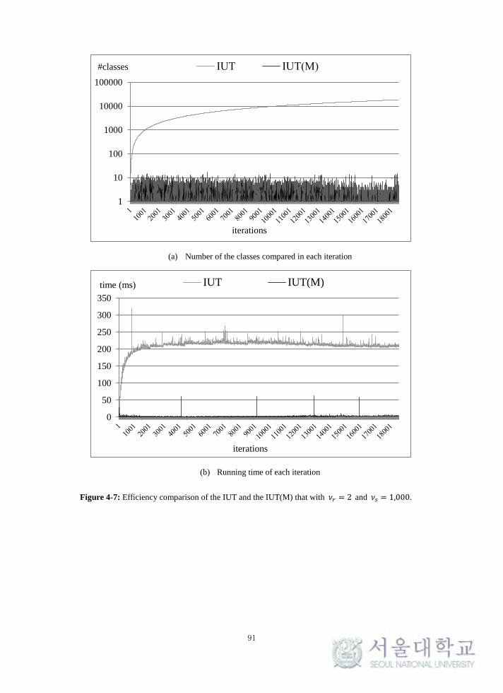
91
(a) Number of the classes compared in each iteration
(b) Running time of each iteration
Figure 4-7: Efficiency comparison of the IUT and the IUT(M) that with 𝜈𝑟 = 2 and 𝜈𝑠 = 1,000.
1
10
100
1000
10000
100000
IUT IUT(M)#classes
iterations
0
50
100
150
200
250
300
350
IUT IUT(M)
iterations
time (ms)
92
4.4 Discussions
The IUT uses Jaccard similarity to calculate the similarity between two classes.
Therefore, the IUT(M) scales the computations of IUT based on MinHash functions
in LSH. However, there are other similarity calculation methods with corresponding
scaling algorithms in LSH. (Duan et al., 2012) applied MinHash and Random
Hyperplane to scale the Jaccard and Cosine similarities used in class similarity
computations. The future work will try to apply Cosine similarity and Random
Hyperplane to the IUT for similarity computations and scaling. The author also
noticed that scaling pair-wise similarity computations in other domains can also
potentially be adapted into schema alignment. These methods, such as parallel
computing based on MapReduce (Lin, 2009; Y. Wang et al., 2013), and
index-based method (Bayardo et al., 2007), are capable of being generalized to
other similarity measures, including Jaccard, Cosine, Overlap, and Dice similarities,
and can be used to improve the IUT in the future works.
93
4.5 Conclusion
Scaling pair-wise similarity computations for classes is vital for schema alignment
in Linked Data that has a large number of instances for classes. In this chapter, the
author introduced a scaling method for the IUT based on LSH to handle the
scalability problem in schema alignment. The proposed method called IUT(M),
which decreases the computations of the IUT when it generates the virtual graph
from two aspects: (1) the similarity computation for each pair of classes is decreased
with MinHash functions, and (2) the number of similarity computations that find the
most similar class for a de-queued class from the class-relation multi-graph are
decreased by using the banding method in LSH. The author performed the IUT(M)
with YAGO2-YAGO2 intra-subsumption alignment task. The experiment shows
that the running time of IUT can be reduced by 94% with a 5% loss in F-score.
94
5 Unsupervised Hierarchical Schema Structure
Generation in Linked Data
5.1 Introduction
The growing needs of RDF resources push organizations to publish their own RDF
format data by transforming their legacy data, such as relational database or Web
pages, with transformation programs (Bizer, 2011; Blum & Cohen, 2010; Ding et
al., 2010; Martín & Gutierrez, 2009). Lacking domain experts to build ontologies,
these data, containing a limited schema but abundant relationships between
instances, are incomplete (Zhu et al., 2015). Without expressive T-Box of an
ontology to describe the relations between concepts, Linked Data suffers in
knowledge acquisition (Zhu et al., 2015).
There are two ways to solve the problem: (1) map instances to an existing
ontology (Bizer et al., 2009; Sahoo et al., 2009); and (2) generate an ontology
directly from data sources (Alani et al., 2003; Mitchell, Betteridge, Carlson,
Hruschka, & Wang, 2009; Pivk, 2006; Tho, Hui, Fong, & Cao, 2006; Tijerino,
Embley, Lonsdale, Ding, & Nagy, 2005). However, it is not desirable to squeeze
every RDF repository under a single ontology, nor for unwilling data providers to
make their Linked Data adhere to any published ontology. The T-Box learned
from the A-box can fully describe the local data set and better represents the
knowledge induced from the instances (Völker & Niepert, 2011). Therefore,
learning T-box from A-box for Linked Data has been studied in the past few years,
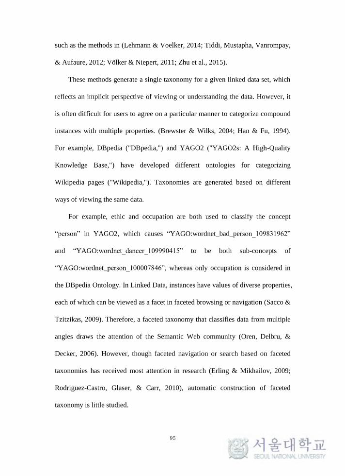
95
such as the methods in (Lehmann & Voelker, 2014; Tiddi, Mustapha, Vanrompay,
& Aufaure, 2012; Völker & Niepert, 2011; Zhu et al., 2015).
These methods generate a single taxonomy for a given linked data set, which
reflects an implicit perspective of viewing or understanding the data. However, it
is often difficult for users to agree on a particular manner to categorize compound
instances with multiple properties. (Brewster & Wilks, 2004; Han & Fu, 1994).
For example, DBpedia ("DBpedia,") and YAGO2 ("YAGO2s: A High-Quality
Knowledge Base,") have developed different ontologies for categorizing
Wikipedia pages ("Wikipedia,"). Taxonomies are generated based on different
ways of viewing the same data.
For example, ethic and occupation are both used to classify the concept
“person” in YAGO2, which causes “YAGO:wordnet_bad_person_109831962”
and “YAGO:wordnet_dancer_109990415” to be both sub-concepts of
“YAGO:wordnet_person_100007846”, whereas only occupation is considered in
the DBpedia Ontology. In Linked Data, instances have values of diverse properties,
each of which can be viewed as a facet in faceted browsing or navigation (Sacco &
Tzitzikas, 2009). Therefore, a faceted taxonomy that classifies data from multiple
angles draws the attention of the Semantic Web community (Oren, Delbru, &
Decker, 2006). However, though faceted navigation or search based on faceted
taxonomies has received most attention in research (Erling & Mikhailov, 2009;
Rodriguez-Castro, Glaser, & Carr, 2010), automatic construction of faceted
taxonomy is little studied.
96
Consequently, in order to meet different needs arising from various uses of
taxonomies, the author proposes a robust method for generating faceted
taxonomies based on object properties of instances in Linked Data. Please note,
different with the taxonomy defined in Chapter 3 and Chapter 4, the taxonomy
used in this chapter has hierarchical structure that only contains the subsumption
relation. There are three benefits of using faceted taxonomy :
(1). Faceted view of the taxonomy facilitates user experience of taxonomy
navigation, since it provides guided navigation of the data organized as a
taxonomy. Other taxonomy generation methods may have such views implicitly
built into their taxonomies, leaving users with no direct exposure to such guidance.
(2). Update of taxonomy is modular in that when an object property is added, a new
sub-taxonomy in a new facet needs to be added into the existing faceted taxonomy
without disrupting existing sub-taxonomies in other facets.
(3). Flexibility in facet combination. Facets can be assembled easily, invoking
rapid filtering of instances. Classifications based on facets can cope with
high-stress tasks, due to its flexibility, especially so when compared with
taxonomies built in a single linear hierarchy.
The author has developed a framework that dynamically extracts data with a single
object property to generate a sub-taxonomy in each facet. Each sub-taxonomy is
generated with an Instance-based Concept Taxonomy generation algorithm called
ICT, adapted from an instance-based ontology alignment algorithm (Zong et al.,
2015). In an addition, the strategies of instantiation and refinement are also
proposed. The experiment comprises two tasks: (1) the construction performance
97
of a sub-taxonomy is tested by comparing the generated taxonomy based on
“rdf:type” with two gold standards, DBpedia and YAGO2, and (2) the
construction performance of a faceted taxonomy with multiple facets is evaluated
by the running time and search effectiveness of the taxonomies based on two
biomedical linked data sets, Diseasome ("Diseasome,") and DrugBank
("DrugBank,"). The two tasks demonstrate the capability of the proposed method
to generate a faceted taxonomy efficiently and effectively.
The rest of the chapter is organized as follows: Section 5.2 gives the basic
principle of the proposed solution; Section 5.3 details on the framework of the
proposed solution; Section 5.4 presents the method of faceted taxonomy
generation; in Sections 5.5 and 5.6, the author demonstrates the results of the
experiments; Section 5.7 discusses limitations of this study and the conclusions are
presented in Section 5.8.
98
5.2 Faceted Taxonomy for Linked Data
Figure 5-1. A faceted taxonomy for a sample of Linked Data.
The object of this study is to automatically construct a concept taxonomy that fully
describes instances. Considering that different instances in the same topic may
have same values of properties, the author is trying to use the property values to
cluster the instances and formalize a concept hierarchy structure. There are two
types of properties in Linked Data sets: data-type and object-type. Object-type
properties link instances with objects, and data-type properties link instance with
literal values (Bechhofer et al., 2004). Please note, given a subject-property-object
(SPO) triple in an A-box, the subject is considered as an instance. If the object is a
literal value, the property is a data-type property. If the object is a de-referenceable
URL, the property is an object-type property, and the URL is called an object
entity or object for short. The author uses the object-type instead of using
data-type property with following reasons. First, instances belonging to the same
concepts may share the same objects and inherit some objects from the super
concept, which is hardly observed on the values of data-type properties. Second,
clustering of instances based on the semantic similarities rather than on lexical
…
A faceted taxonomy
…
facet k: Symptom (T-Box)
(A-Box)
Diabetes
mellitus type 2
facet 1: Cause
Trisomy 21 Down
syndrome
Urinary
System
Frequent
urination
Neurological
Speech
disturbance
Acquired
Factors
Genetic
Hereditary ObeseNon-
hereditary
Translocation
Down syndrome
Symptom
Taxonomy
Generation
Instantiation
Diseases in Linked DataSub-Data
Sub-Data
…
Facet k
Facet 1
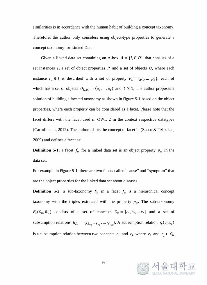
99
similarities is in accordance with the human habit of building a concept taxonomy.
Therefore, the author only considers using object-type properties to generate a
concept taxonomy for Linked Data.
Given a linked data set containing an A-box 𝐴 = {𝐼, 𝑃, 𝑂} that consists of a
set instances 𝐼, a set of object properties 𝑃 and a set of objects 𝑂, where each
instance 𝑖𝑢 ∈ 𝐼 is described with a set of property 𝑃𝑢 = {𝑝1, … , 𝑝𝑘}, each of
which has a set of objects 𝑂𝑖𝑢𝑝𝑣 = {𝑜1, … , 𝑜𝑡} and 𝑡 ≥ 1, The author proposes a
solution of building a faceted taxonomy as shown in Figure 5-1 based on the object
properties, where each property can be considered as a facet. Please note that the
facet differs with the facet used in OWL 2 in the context respective datatypes
(Carroll et al., 2012). The author adapts the concept of facet in (Sacco & Tzitzikas,
2009) and defines a facet as:
Definition 5-1: a facet 𝑓𝑢 for a linked data set is an object property 𝑝𝑢 in the
data set.
For example in Figure 5-1, there are two facets called “cause” and “symptom” that
are the object properties for the linked data set about diseases.
Definition 5-2: a sub-taxonomy 𝐹𝑢 in a facet 𝑓𝑢 is a hierarchical concept
taxonomy with the triples extracted with the property 𝑝𝑢. The sub-taxonomy
𝐹𝑢(𝐶𝑢, 𝑅𝑢) consists of a set of concepts 𝐶𝑢 = {𝑐1, 𝑐2, … 𝑐𝑡} and a set of
subsumption relations 𝑅𝑆𝑢 = {𝑟𝑆𝑢1 , 𝑟𝑆𝑢2 , … 𝑟𝑆𝑢𝑥}. A subsumption relation 𝑟𝑠(𝑐𝑖, 𝑐𝑗)
is a subsumption relation between two concepts 𝑐𝑖 and 𝑐𝑗, where 𝑐𝑖 and 𝑐𝑗 ∈ 𝐶𝑢.
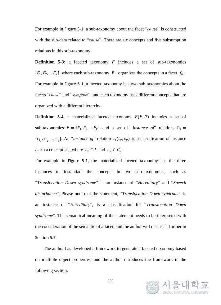
100
For example in Figure 5-1, a sub-taxonomy about the facet “cause” is constructed
with the sub-data related to “cause”. There are six concepts and five subsumption
relations in this sub-taxonomy.
Definition 5-3: a faceted taxonomy 𝐹 includes a set of sub-taxonomies
{𝐹1, 𝐹2, …𝐹𝑘}, where each sub-taxonomy 𝐹𝑢 organizes the concepts in a facet 𝑓𝑢.
For example in Figure 5-1, a faceted taxonomy has two sub-taxonomies about the
facets “cause” and “symptom”, and each taxonomy uses different concepts that are
organized with a different hierarchy.
Definition 5-4: a materialized faceted taxonomy ℱ(𝐹, 𝑅) includes a set of
sub-taxonomies 𝐹 = {𝐹1, 𝐹2, …𝐹𝑘} and a set of “instance of” relations RI =
{rI1 , rI2 , … rIe}. An “instance of” relation 𝑟𝐼(𝑖𝑢, 𝑐𝑣) is a classification of instance
𝑖𝑢 to a concept 𝑐𝑣, where 𝑖𝑢 ∈ 𝐼 and 𝑐𝑣 ∈ 𝐶𝑢.
For example in Figure 5-1, the materialized faceted taxonomy has the three
instances to instantiate the concepts in two sub-taxonomies, such as
“Translocation Down syndrome” is an instance of “Hereditary” and “Speech
disturbance”. Please note that the statement, “Translocation Down syndrome” is
an instance of “Hereditary”, is a classification for “Translocation Down
syndrome”. The semantical meaning of the statement needs to be interpreted with
the consideration of the semantic of a facet, and the author will discuss it further in
Section 5.7.
The author has developed a framework to generate a faceted taxonomy based
on multiple object properties, and the author introduces the framework in the
following section.
101
5.3 Framework
Figure 5-2. The framework of faceted taxonomy construction.
The author separates the procedure of generating a faceted taxonomy into two
stages as shown in Figure 5-2: pre-processing and taxonomical relationship
generation.
The pre-processing is to generate a set of instance-object matrices, each of
which represents the relations between instances in one facet (object property).
Four steps, (1) facets extraction, (2) instance restriction and redundancy removal,
(3) redundant object removal, and (4) instance-object matrix generation, are used
at this stage in order to remove redundant instances and objects for reducing the
computations of sub-taxonomy generation.
The taxonomical relationship generation is to construct sub-taxonomies based
on instance-object matrices generated from multiple facets. For each matrix, the
author proposes an algorithm to build a hierarchical taxonomy. An instantiation
and concept taxonomy refinement strategies are also proposed to get a
materialized faced taxonomy in Section 5.4.
Facets
Extraction
Instance Restriction and
Redundancy Removal
Sub-concept
Taxonomies
Construction
Materialized Faceted
Taxonomy
Linked Data Sets
Pre-Processing
Taxonomical Relationship Generation
1
2
Instance-Object
Matrix Generation
Instantiation and
taxonomies refinement
Redundant Objects
Removal
Redundant Instances
for each facet
Redundant Objects
for each facet
Instance-Objects
Matrices
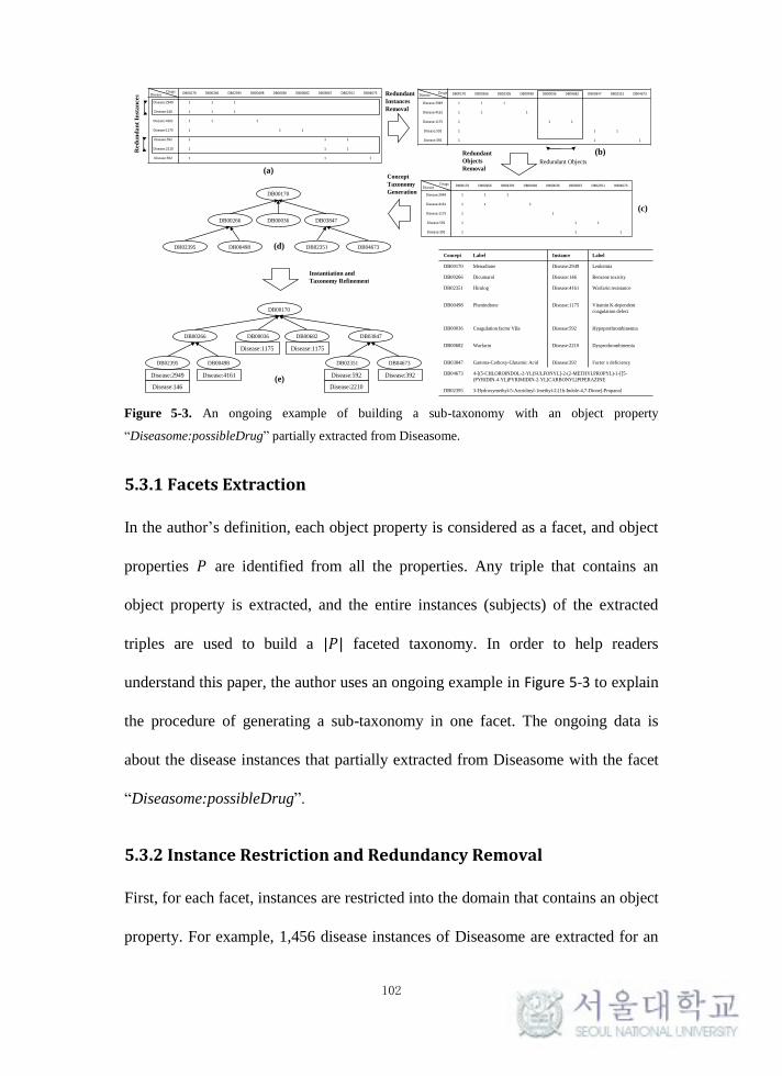
102
Figure 5-3. An ongoing example of building a sub-taxonomy with an object property
“Diseasome:possibleDrug” partially extracted from Diseasome.
5.3.1 Facets Extraction
In the author’s definition, each object property is considered as a facet, and object
properties 𝑃 are identified from all the properties. Any triple that contains an
object property is extracted, and the entire instances (subjects) of the extracted
triples are used to build a |𝑃| faceted taxonomy. In order to help readers
understand this paper, the author uses an ongoing example in Figure 5-3 to explain
the procedure of generating a sub-taxonomy in one facet. The ongoing data is
about the disease instances that partially extracted from Diseasome with the facet
“Diseasome:possibleDrug”.
5.3.2 Instance Restriction and Redundancy Removal
First, for each facet, instances are restricted into the domain that contains an object
property. For example, 1,456 disease instances of Diseasome are extracted for an
DB00170
DB00266 DB00036 DB03847
DB02395 DB00498 DB02351 DB04673
Concept Label Instance Label
DB00170 Menadione Disease:2949 Leukemia
DB00266 Dicumarol Disease:146 Benzene toxicity
DB02351 Hirulog Disease:4161 Warfarin resistance
DB00498 Phenindione Disease:1175 Vitamin K-dependent
coagulation defect
DB00036 Coagulation factor VIIa Disease:592 Hypoprothrombinemia
DB00682 Warfarin Disease:2210 Dysprothrombinemia
DB03847 Gamma-Carboxy-Glutamic Acid Disease:392 Factor x deficiency
DB04673 4-[(5-CHLOROINDOL-2-YL)SULFONYL]-2-(2-METHYLPROPYL)-1-[[5-
(PYRIDIN-4-YL)PYRIMIDIN-2-YL]CARBONYL]PIPERAZINE
DB02395 3-Hydroxymethyl-5-Aziridinyl-1methyl-2-[1h-Indole-4,7-Dione]-Propanol
DB00170 DB00266 DB02395 DB00498 DB00036 DB00682 DB03847 DB02351 DB04673
Disease:2949 1 1 1
Disease:146 1 1 1
Disease:4161 1 1 1
Disease:1175 1 1 1
Disease:592 1 1 1
Disease:2210 1 1 1
Disease:392 1 1 1
DB00170 DB00266 DB02395 DB00498 DB00036 DB00682 DB03847 DB02351 DB04673
Disease:2949 1 1 1
Disease:4161 1 1 1
Disease:1175 1 1 1
Disease:592 1 1 1
Disease:392 1 1 1R
ed
un
da
nt
Inst
an
ces Redundant
Instances
Removal
Redundant Objects
Instantiation and
Taxonomy Refinement
DB00170 DB00266 DB02395 DB00498 DB00036 DB03847 DB02351 DB04673
Disease:2949 1 1 1
Disease:4161 1 1 1
Disease:1175 1 1
Disease:592 1 1 1
Disease:392 1 1 1
Concept
Taxonomy
Generation
DB00170
DB00266 DB00036 DB03847
DB02395 DB00498 DB02351 DB04673
DB00682
Disease:2949
Disease:146
Disease:4161
Disease:1175 Disease:1175
Disease:592
Disease:2210
Disease:392
Redundant
Objects
Removal
DrugsDisease
Drugs
Drugs
Disease
Disease
(a)
(b)
(c)
(d)
(e)
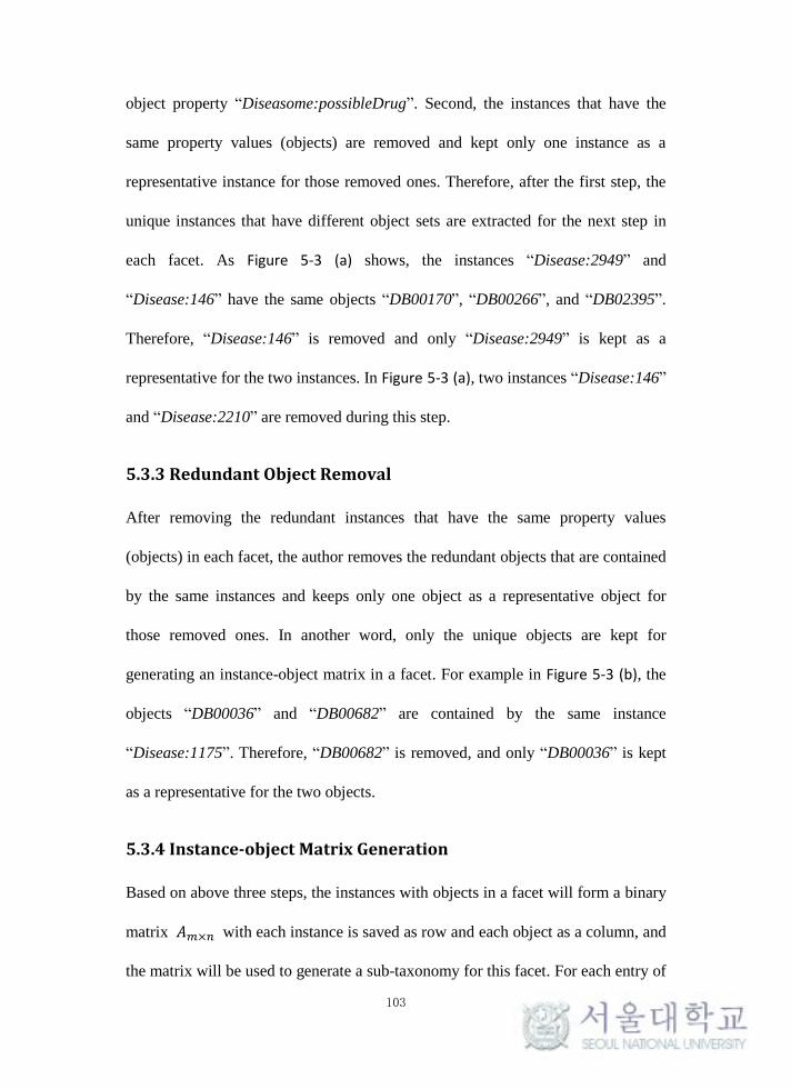
103
object property “Diseasome:possibleDrug”. Second, the instances that have the
same property values (objects) are removed and kept only one instance as a
representative instance for those removed ones. Therefore, after the first step, the
unique instances that have different object sets are extracted for the next step in
each facet. As Figure 5-3 (a) shows, the instances “Disease:2949” and
“Disease:146” have the same objects “DB00170”, “DB00266”, and “DB02395”.
Therefore, “Disease:146” is removed and only “Disease:2949” is kept as a
representative for the two instances. In Figure 5-3 (a), two instances “Disease:146”
and “Disease:2210” are removed during this step.
5.3.3 Redundant Object Removal
After removing the redundant instances that have the same property values
(objects) in each facet, the author removes the redundant objects that are contained
by the same instances and keeps only one object as a representative object for
those removed ones. In another word, only the unique objects are kept for
generating an instance-object matrix in a facet. For example in Figure 5-3 (b), the
objects “DB00036” and “DB00682” are contained by the same instance
“Disease:1175”. Therefore, “DB00682” is removed, and only “DB00036” is kept
as a representative for the two objects.
5.3.4 Instance-object Matrix Generation
Based on above three steps, the instances with objects in a facet will form a binary
matrix 𝐴𝑚×𝑛 with each instance is saved as row and each object as a column, and
the matrix will be used to generate a sub-taxonomy for this facet. For each entry of

104
the matrix, 𝑎𝑢𝑣 = 1 if the instance 𝑢 contains the object 𝑣 . There are |𝑃|
matrices for all object properties 𝑃, and each matrix has different number of
instances and objects. In the example of Figure 5-3 (c), for the facet
“Diseasome:possibleDrug”, the instance-object matrix that has a five (instances)
by eight (objects) matrix is generated.
105
5.4 Generating Faceted Taxonomy
5.4.1 The Problem of Generating a Sub-taxonomy for a Facet
The author’s object is to obtain a faceted taxonomy that contains sub-taxonomies
generated with instance-object matrices. Therefore, for each facet, the author
defines the basic problem of building a hierarchical taxonomy in one facet as
follows:
Input: Given an instance-object matrix 𝐴𝑚×𝑛 that contains the instances with
multiple values (objects), we obtain an instance set 𝐼 = {𝑖1, 𝑖2, … , 𝑖𝑚} that have
𝑚 instances and an object set 𝑂 = {𝑜1, 𝑜2, … , 𝑜𝑛} that have 𝑛 objects. For each
instance 𝑖𝑘, an instance contains by a set of objects {𝑜1, 𝑜2, … , 𝑜𝑢}. For example
in Figure 5-3 (c), the instance “Disease:2949” contains the objects “DB00170”,
“DB00266”, and “DB02395”.
Output: A hierarchical concept taxonomy 𝐹 (𝐶, 𝑅𝑠), where 𝐶 = {𝑐1, 𝑐2, … , 𝑐𝑘}
is a concept set containing 𝑘 concepts, 𝑅𝑠 = {𝑟𝑠1 , 𝑟𝑠2 , … , 𝑟𝑠𝑖} a subsumption
relation set for the concepts.
5.4.2 Concept Definition and Naming
Classes (concepts) provide an abstraction mechanism to generalize the
characteristics of a group of similar instances. The instances in a class are
extensions that can be used to define the class (Bechhofer et al., 2004). The author
defines a class with extensions (i.e., a set of instance) as :
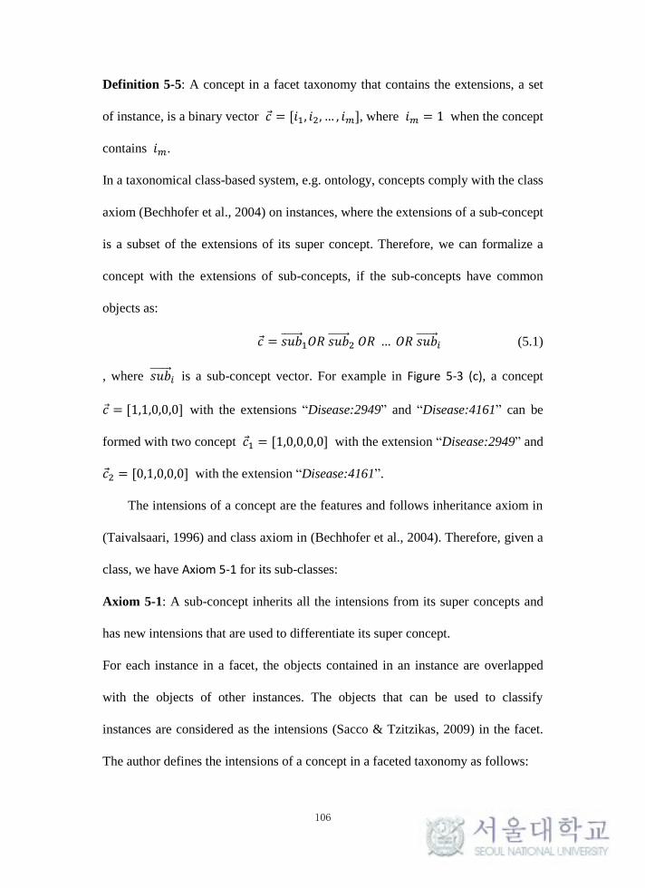
106
Definition 5-5: A concept in a facet taxonomy that contains the extensions, a set
of instance, is a binary vector 𝑐 = [𝑖1, 𝑖2, … , 𝑖𝑚], where 𝑖𝑚 = 1 when the concept
contains 𝑖𝑚.
In a taxonomical class-based system, e.g. ontology, concepts comply with the class
axiom (Bechhofer et al., 2004) on instances, where the extensions of a sub-concept
is a subset of the extensions of its super concept. Therefore, we can formalize a
concept with the extensions of sub-concepts, if the sub-concepts have common
objects as:
𝑐 = 𝑠𝑢𝑏⃗⃗⃗⃗⃗⃗⃗⃗1𝑂𝑅 𝑠𝑢𝑏⃗⃗⃗⃗⃗⃗⃗⃗
2 𝑂𝑅 … 𝑂𝑅 𝑠𝑢𝑏⃗⃗⃗⃗⃗⃗⃗⃗𝑖 (5.1)
, where 𝑠𝑢𝑏⃗⃗⃗⃗⃗⃗⃗⃗𝑖 is a sub-concept vector. For example in Figure 5-3 (c), a concept
𝑐 = [1,1,0,0,0] with the extensions “Disease:2949” and “Disease:4161” can be
formed with two concept 𝑐1 = [1,0,0,0,0] with the extension “Disease:2949” and
𝑐2 = [0,1,0,0,0] with the extension “Disease:4161”.
The intensions of a concept are the features and follows inheritance axiom in
(Taivalsaari, 1996) and class axiom in (Bechhofer et al., 2004). Therefore, given a
class, we have Axiom 5-1 for its sub-classes:
Axiom 5-1: A sub-concept inherits all the intensions from its super concepts and
has new intensions that are used to differentiate its super concept.
For each instance in a facet, the objects contained in an instance are overlapped
with the objects of other instances. The objects that can be used to classify
instances are considered as the intensions (Sacco & Tzitzikas, 2009) in the facet.
The author defines the intensions of a concept in a faceted taxonomy as follows:
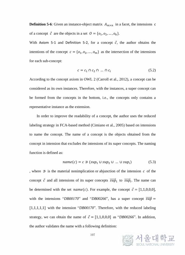
107
Definition 5-6: Given an instance-object matrix 𝐴𝑚×𝑛 in a facet, the intensions c
of a concept 𝑐 are the objects in a set 𝑂 = {𝑜1, 𝑜2, … , 𝑜𝑘}.
With Axiom 5-1 and Definition 5-2, for a concept 𝑐, the author obtains the
intentions of the concept 𝑐 = {𝑜1, 𝑜2, … , 𝑜𝑚} as the intersection of the intensions
for each sub-concept:
𝑐 = 𝑐1 ∩ 𝑐2 ∩ … ∩ 𝑐𝑖 (5.2)
According to the concept axiom in OWL 2 (Carroll et al., 2012), a concept can be
considered as its own instances. Therefore, with the instances, a super concept can
be formed from the concepts in the bottom, i.e., the concepts only contains a
representative instance as the extension.
In order to improve the readability of a concept, the author uses the reduced
labeling strategy in FCA-based method (Cimiano et al., 2005) based on intensions
to name the concept. The name of a concept is the objects obtained from the
concept in intension that excludes the intensions of its super concepts. The naming
function is defined as:
𝑛𝑎𝑚𝑒(𝑐) = 𝑐 ⊅ (𝑠𝑢𝑝1 ∪ 𝑠𝑢𝑝2 ∪ … ∪ 𝑠𝑢𝑝𝑖) (5.3)
, where ⊅ is the material nonimplication or abjunction of the intension 𝑐 of the
concept 𝑐 and all intensions of its super concepts 𝑠𝑢𝑝⃗⃗⃗⃗⃗⃗⃗⃗ 1 to 𝑠𝑢𝑝⃗⃗⃗⃗⃗⃗⃗⃗ 𝑖. The name can
be determined with the set 𝑛𝑎𝑚𝑒(𝑐). For example, the concept 𝑐 = [1,1,0,0,0],
with the intensions “DB00170” and “DB00266”, has a super concept 𝑠𝑢𝑝⃗⃗⃗⃗⃗⃗⃗⃗ =
[1,1,1,1,1] with the intension “DB00170”. Therefore, with the reduced labeling
strategy, we can obtain the name of 𝑐 = [1,1,0,0,0] as “DB00266”. In addition,
the author validates the name with a following definition:
108
Definition 5-7: A concept 𝑐 is valid only if |𝑛𝑎𝑚𝑒(𝑐)| = 1.
This definition makes the proposed method differ with other taxonomy generation
algorithms, such as the FCA. With Definition 5-7, the proposed taxonomy
generation algorithm is more efficient and more effective than the FCA, which
will be discussed in Section 5.6.1.
5.4.3 Taxonomy Generation Algorithm
With the concept definition and the naming strategy, the author adapts the IUT
(Zong et al., 2015) that can be used to generate a taxonomy based on
instance-concept matrix, and call the variation ICT (a.k.a., Instance-based
hierarchical Concept Taxonomy generation). There are two steps to generate the
concept taxonomy: first, the objects in the matrix 𝐴𝑚×𝑛 are sorted in descending
order by the number of instances contained by the object, and are put into a queue
𝑄 (line 1 in Algorithm 5-1); second, in each iteration, a concept is de-queued and
put onto the right position in a graph by computing the subsumption relation with
existing concepts (lines 3-9 in Algorithm 5-1). The author adapts the equation in
(Sanderson & Croft, 1999) to determine a subsumption relation between two
concepts 𝑐𝑢 and 𝑐𝑣 (𝑐𝑢 is a sub-concept of 𝑐𝑣) as follows:
𝑠𝑢𝑏(𝑐𝑢, 𝑐𝑣) =|𝑐𝑢 ∩ 𝑐𝑣|
|𝑐𝑢| ≥ 𝜑 , 𝑠𝑢𝑏(𝑐𝑣 , 𝑐𝑢) =
|𝑐𝑣 ∩ 𝑐𝑢|
|𝑐𝑣|< 1 (5.4)
, where 𝜑 is used to adjust the effectiveness of subsumption determination for the
two concepts.
If a concept 𝑐𝑢 has two super concepts, where exists a path from one concept
to the other (i.e., one concept is the ancestor of the other), the concept will be
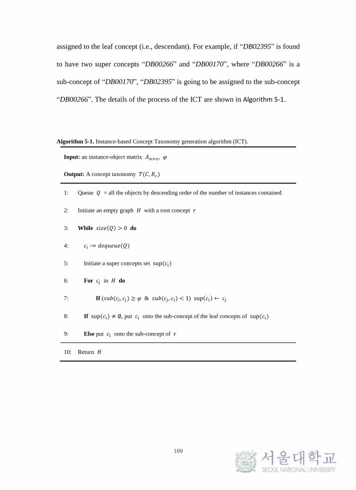
109
assigned to the leaf concept (i.e., descendant). For example, if “DB02395” is found
to have two super concepts “DB00266” and “DB00170”, where “DB00266” is a
sub-concept of “DB00170”, “DB02395” is going to be assigned to the sub-concept
“DB00266”. The details of the process of the ICT are shown in Algorithm 5-1.
Algorithm 5-1. Instance-based Concept Taxonomy generation algorithm (ICT).
Input: an instance-object matrix 𝐴𝑚×𝑛, 𝜑
Output: A concept taxonomy 𝑇(𝐶, 𝑅𝑐)
1: Queue 𝑄 = all the objects by descending order of the number of instances contained
2: Initiate an empty graph 𝐻 with a root concept 𝑟
3: While 𝑠𝑖𝑧𝑒(𝑄) > 0 do
4: 𝑐𝑖 ∶= 𝑑𝑒𝑞𝑢𝑒𝑢𝑒(𝑄)
5: Initiate a super concepts set sup (𝑐𝑖)
6: For 𝑐𝑗 in 𝐻 do
7: If (𝑠𝑢𝑏(𝑐𝑖 , 𝑐𝑗) ≥ 𝜑 & 𝑠𝑢𝑏(𝑐𝑗 , 𝑐𝑖) < 1) sup(𝑐𝑖) ← 𝑐𝑗
8: If sup (𝑐𝑖) ≠ ∅, put 𝑐𝑖 onto the sub-concept of the leaf concepts of sup (𝑐𝑖)
9: Else put 𝑐𝑖 onto the sub-concept of 𝑟
10: Return 𝐻
110
5.4.4 Instantiation and Taxonomy Refinement
In this step, the author needs to materialize the faceted taxonomy based on
multiple sub-taxonomies generated. First, the author instantiates the concepts in
each sub-taxonomy. The author defines a following instantiation rule based on an
instance-object matrix.
Rule 5-1: If an instance belongs to two concepts 𝑐𝑢 and 𝑐𝑣, where 𝑐𝑢 is the
super concept of 𝑐𝑣, the instance will be used to populate 𝑐𝑣.
Rule 5-1 makes an instance populate leaf nodes in a sub-taxonomy. For example,
the instance “Disease:1175” belongs to two concepts “DB00036” and “DB00170”
in Figure 5-3, and “Disease:1175” will be assigned to the concept “DB00036”
since “DB00036” is the sub-concept of “DB00170”. Notice that Rule 5-1 supports
multiple instantiation, because if an instance belongs to two concepts that are not
connected with a subsumption relation, the instance will be assigned equally to the
two concepts.
Second, the removed redundant instances and objects in the pre-processing
stage are used to refine the taxonomy. The redundant instances are used to
populate the same concepts instantiated with the representative instances. For
example, “Disease:146” is assigned to the concept “DB02395” as well since
“DB02395” is instantiated with “Disease:2949”. The redundant objects are
considered equivalent with the representative objects in the taxonomy. For
example, the concept “DB00682” is also considered as a sub-concept of the
concept “DB00170” since “DB00036” is the sub-concept of “DB00170”.
111
Third, assemble all sub-taxonomies with renamed concepts. Each
sub-taxonomy should be independent and contains different concepts. However,
there are cases that objects in the same topic may be used in different object
properties. For example, the objects typed “DrugBank:references” are used in both
object properties “DrugBank:drugReference” and “DrugBank:generalReference”
for the instances typed “DrugBank:targets”. Therefore, in order to disjoint all the
facet concepts, the author prefixes each concept name with the name of the
property in a facet (Sacco & Tzitzikas, 2009). Finally, the author puts all the
sub-taxonomies under the concept “Owl:Thing” to get the faceted taxonomy.
112
5.5 Experiments
The author has implemented the proposed method based on JDK 1.6 using an
Intel(R) Xeon CPU E5-2630 with 130 GB RAM on Windows 8 64 bit version.
Since the object is to construct faceted taxonomies for Linked Data, the tests are
separated into two parts that target two problems the author mentioned in Sections
5.4.1 and 5.2.2: (1) the performance of generating a sub-taxonomy in one facet. (2)
the performance of generating multiple faceted taxonomies with different object
properties.
5.5.1 Task 1-Construction of Taxonomy with “rdf:type”
5.5.1.1 Data Sets and Experiment Design
In Linked Data, some data sets that contain ontologies with concept taxonomies
publish the classification of instances with “rdf:type”. Generating taxonomies with
“rdf:type” can be viewed as the reverse engineering of this RDF publishing.
Therefore, in order to evaluate the performance of the proposed method to build a
sub-taxonomy with one object property, the author used the values of “rdf:type” in
the RDF dumping file to construct a taxonomy. The taxonomy will be evaluated
by comparing with the taxonomy of the gold standard ontology. The author chose
two most well-known sets in LOD, DBpedia ("Downloads - Dbpedia,") and
YAGO2 ("Downloads - YAGO2,") that provide the mature concept taxonomies
reflecting on the values of “rdf:type”. The concept taxonomies are DBpedia
ontology and YAGO-WordNet, which are extracted from DBpedia and YAGO2
respectively. The author gained the study population, with 2,885,951 instance and
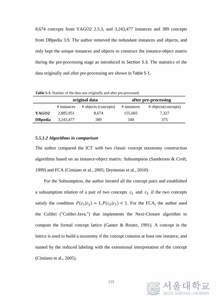
113
8,674 concepts from YAGO2 2.5.3, and 3,243,477 instances and 389 concepts
from DBpedia 3.9. The author removed the redundant instances and objects, and
only kept the unique instances and objects to construct the instance-object matrix
during the pre-processing stage as introduced in Section 5.3. The statistics of the
data originally and after pre-processing are shown in Table 5-1.
Table 5-1. Statistic of the data sets originally and after pre-processed.
original data after pre-processing
# instances # objects (concepts) # instances # objects(concepts)
YAGO2 2,885,951 8,674 155,602 7,327
DBpedia 3,243,477 389 348 375
5.5.1.2 Algorithms in comparison
The author compared the ICT with two classic concept taxonomy construction
algorithms based on an instance-object matrix: Subsumption (Sanderson & Croft,
1999) and FCA (Cimiano et al., 2005; Drymonas et al., 2010).
For the Subsumption, the author iterated all the concept pairs and established
a subsumption relation of a pair of two concepts 𝑐1 and 𝑐2 if the two concepts
satisfy the condition 𝑃(𝑐1|𝑐2) = 1, 𝑃(𝑐2|𝑐1) < 1. For the FCA, the author used
the Colibri ("Colibri-Java,") that implements the Next-Closure algorithm to
compute the formal concept lattice (Ganter & Reuter, 1991). A concept in the
lattice is used to build a taxonomy if the concept contains at least one instance, and
named by the reduced labeling with the extensional interpretation of the concept
(Cimiano et al., 2005).
114
5.5.1.3 Evaluation Criteria
The author tested all the algorithms with two criteria: efficiency and effectiveness.
For evaluating the effectiveness, the author compared a generated taxonomy with
the hierarchical schema structure of the ontology already exist in a linked data set.
The author adopted the Taxonomic Precision (TP), Taxonomic Recall (TR), and
Taxonomic F-measure (Dellschaft & Staab, 2006; Paukkeri et al., 2012) to
measure the quality of the generated taxonomy.
TP and TR are based on the Semantic Cotopy (SC) (Dellschaft & Staab, 2006)
that considers ancestor and descendant relation to calculate the similarity of two
concepts. The Semantic Cotopy of a concept 𝑐 in an ontology 𝑂 is defined as:
𝑆𝐶(𝑐, 𝑂) = {𝑐𝑖|𝑐𝑖 ∈ 𝐶 ∧ (𝑐𝑖 ≤ 𝑐 ⋁ 𝑐 ≥ 𝑐𝑖)} (5.5)
, where 𝐶 is the concept set of 𝑂 , and 𝑐𝑖 ≤ 𝑐 ⋁ 𝑐 ≥ 𝑐𝑖 is an ancestor and
descendant of 𝑐. Therefore, the semantic cotopy of two concepts can be used to
compute the local taxonomic precision of the two concepts as follows:
𝑡𝑝𝑠𝑐(𝑐1, 𝑐2, 𝑂1, 𝑂2) =|𝑠𝑐(𝑐1,𝑂1)∩𝑠𝑐(𝑐2,𝑂2)|
|𝑠𝑐(𝑐1,𝑂1)| (5.6)
The 𝑇𝑃𝑆𝐶 and 𝑇𝑅𝑆𝐶 are computed based on the local taxonomic precisions
and recalls as follows:
𝑇𝑃𝑆𝐶(𝑂1, 𝑂2) =1
|𝐶𝑂1|∑ {
𝑡𝑝𝑠𝑐(𝑐𝑖, 𝑐𝑖 , 𝑂1, 𝑂2) 𝑖𝑓 𝑐𝑖 ∈ 𝐶𝑂20 𝑖𝑓 𝑐𝑖 ∉ 𝐶𝑂2
𝑐𝑖 ∈ 𝐶𝑂1 (5.7)
, where 𝑇𝑅𝑆𝐶(𝑂1, 𝑂2) = 𝑇𝑃𝐶𝑆𝐶(𝑂2, 𝑂1).
The Taxonomic F-measure (TF) calculates the harmonic mean of 𝑇𝑃𝑆𝐶 and
𝑇𝑅𝑆𝐶 as:
𝑇𝐹(𝑂1, 𝑂2) =2×𝑇𝑅𝑆𝐶(𝑂1,𝑂2)×𝑇𝑃𝑆𝐶(𝑂1,𝑂2)
𝑇𝑅𝑆𝐶(𝑂1,𝑂2)+𝑇𝑃𝑆𝐶(𝑂1,𝑂2) (5.8)
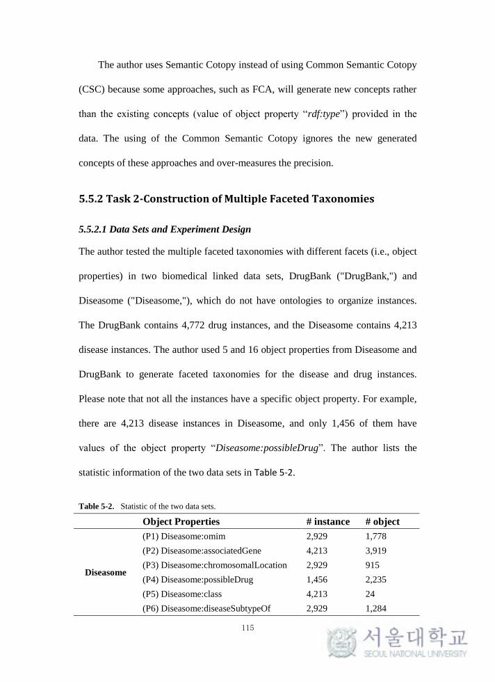
115
The author uses Semantic Cotopy instead of using Common Semantic Cotopy
(CSC) because some approaches, such as FCA, will generate new concepts rather
than the existing concepts (value of object property “rdf:type”) provided in the
data. The using of the Common Semantic Cotopy ignores the new generated
concepts of these approaches and over-measures the precision.
5.5.2 Task 2-Construction of Multiple Faceted Taxonomies
5.5.2.1 Data Sets and Experiment Design
The author tested the multiple faceted taxonomies with different facets (i.e., object
properties) in two biomedical linked data sets, DrugBank ("DrugBank,") and
Diseasome ("Diseasome,"), which do not have ontologies to organize instances.
The DrugBank contains 4,772 drug instances, and the Diseasome contains 4,213
disease instances. The author used 5 and 16 object properties from Diseasome and
DrugBank to generate faceted taxonomies for the disease and drug instances.
Please note that not all the instances have a specific object property. For example,
there are 4,213 disease instances in Diseasome, and only 1,456 of them have
values of the object property “Diseasome:possibleDrug”. The author lists the
statistic information of the two data sets in Table 5-2.
Table 5-2. Statistic of the two data sets.
Object Properties # instance # object
Diseasome
(P1) Diseasome:omim 2,929 1,778
(P2) Diseasome:associatedGene 4,213 3,919
(P3) Diseasome:chromosomalLocation 2,929 915
(P4) Diseasome:possibleDrug 1,456 2,235
(P5) Diseasome:class 4,213 24
(P6) Diseasome:diseaseSubtypeOf 2,929 1,284
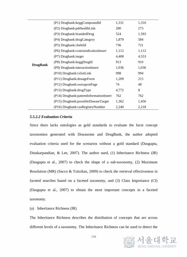
116
DrugBank
(P1) Drugbank:keggCompoundId 1,331 1,316
(P2) Drugbank:pdrhealthLink 280 273
(P3) Drugbank:brandedDrug 524 1,593
(P4) Drugbank:drugCategory 1,879 584
(P5) Drugbank:chebiId 736 721
(P6) Drugbank:contraindicationInsert 1,112 1,112
(P7) Drugbank:target 4,408 4,553
(P8) Drugbank:keggDrugId 913 910
(P9) Drugbank:interactionInsert 1,036 1,036
(P10) Drugbank:rxlistLink 998 994
(P11) Drugbank:dosageForm 1,209 215
(P12) Drugbank:swissprotPage 74 48
(P13) Drugbank:drugType 4,772 8
(P14) Drugbank:patientInformationInsert 762 762
(P15) Drugbank:possibleDiseaseTarget 1,362 1,456
(P16) Drugbank:casRegistryNumber 2,240 2,218
5.5.2.2 Evaluation Criteria
Since there lacks ontologies as gold standards to evaluate the facet concept
taxonomies generated with Diseasome and DrugBank, the author adopted
evaluation criteria used for the scenarios without a gold standard (Dasgupta,
Dinakarpandian, & Lee, 2007). The author used, (1) Inheritance Richness (IR)
(Dasgupta et al., 2007) to check the shape of a sub-taxonomy, (2) Maximum
Resolution (MR) (Sacco & Tzitzikas, 2009) to check the retrieval effectiveness in
faceted searches based on a faceted taxonomy, and (3) Class Importance (CI)
(Dasgupta et al., 2007) to obtain the most important concepts in a faceted
taxonomy.
(a) Inheritance Richness (IR)
The Inheritance Richness describes the distribution of concepts that are across
different levels of a taxonomy. The Inheritance Richness can be used to detect the
117
shape of the concept taxonomy. A low value of Inheritance Richness indicates a
horizontal hierarchy (flat structure) that has a low degree of inheritance level
where each concept has a large number of sub-concepts. A high value of
Inheritance Richness indicates a vertical hierarchy that has a high degree of
inheritance level where each concept has a small number of sub-concepts.
The Inheritance Richness is computed as follows:
𝐼𝑅 =∑ |𝑑𝑒𝑠𝑐𝑒𝑛𝑑(𝐶𝑖)|𝑐𝑖∈𝐶
|𝐶| (5.9)
, where |𝑆𝑢𝑏(𝐶𝑖)| is the cardinality of the set of the descendants a concept 𝑐𝑖.
(b) Maximum Resolution (MR)
Maximum Resolution is used to measure the retrieval effectiveness with a faceted
taxonomy. A Maximum Resolution measures the average minimum number of
instances to be manually inspected after a refinement through operations on the
faceted taxonomy. A small value of Maximum Resolution illustrates a good
classification of a concept taxonomy for reducing the search space. The Maximum
Resolution is computed as the average number of instances of k concept
intersections in a 𝑘 facets taxonomy:
𝑀𝑅 =∑⋂ 𝑐𝑖
𝑘𝑖=1
| ∑⋂ 𝑐𝑖𝑘𝑖=1 |
(5.10)
, where | ∑⋂ 𝑐𝑖𝑘𝑖=1 | is total intersection numbers of 𝑘 concepts, each of which is
a leaf concept from a sub-taxonomy.
(c) Class Importance (CI)
In order to obtain the important classes, the author adapts Class Importance to
show the focused concepts with the consideration of instance distribution and help
118
users to identify where to get data if the intentions of users’ are to get consistent
coverages of all concepts.
The importance of a concept 𝑐𝑖 is computed as follows:
𝐶𝐼(𝑐𝑖) =|𝐼𝑐𝑖|
|𝐼| (5.11)
, where 𝐼𝑐𝑖 is the instance set of 𝑐𝑖. Please note that the instances belonged to 𝑐𝑖
contain all the instances belonged to each sub-concept of the 𝑐𝑖.
119
5.6 Results
5.6.1 Results of Task 1
The author has run three methods over two data sets (YAGO2 and DBpedia)
respectively, and show the running time of all the methods in Figure 5-4 (b). As
Figure 5-4 (b) shows, the ICT is the fastest methods (49 ms for DBpedia and
11,790 ms for YAGO2) comparing with other two methods. The ICT and
Subsumption reduce the search space into the concepts already existing in the
concept taxonomy with Definition 5-7, and the ICT does not need to calculate
Equation 5.4 with all the combinations of the concept pairs that are needed for the
Subsumption (118 ms for DBpedia and 2,597,424 ms for YAGO2). The FCA (184
ms for DBpedia and 92,656,444 ms for YAGO2) is the slowest method since it
calculates all the possible pairs of concepts sharing common instances. The huge
amount of discovered relations from the FCA makes the extraction of subsumption
relations very expensive. In the two tests, over than 55% of the running time is
spent on the extraction of the subsumption relations from all the discovered
relations (103/184 for DBpedia and 90,942,222/92,656,444 for YAGO2).
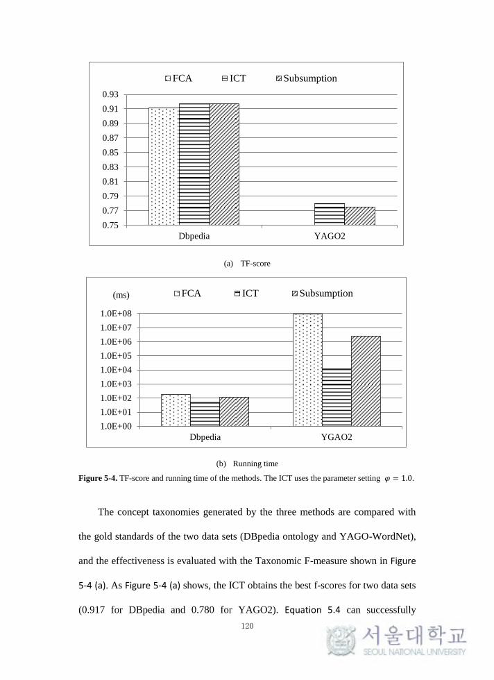
120
(a) TF-score
(b) Running time
Figure 5-4. TF-score and running time of the methods. The ICT uses the parameter setting 𝜑 = 1.0.
The concept taxonomies generated by the three methods are compared with
the gold standards of the two data sets (DBpedia ontology and YAGO-WordNet),
and the effectiveness is evaluated with the Taxonomic F-measure shown in Figure
5-4 (a). As Figure 5-4 (a) shows, the ICT obtains the best f-scores for two data sets
(0.917 for DBpedia and 0.780 for YAGO2). Equation 5.4 can successfully
0.75
0.77
0.79
0.81
0.83
0.85
0.87
0.89
0.91
0.93
Dbpedia YAGO2
FCA ICT Subsumption
1.0E+00
1.0E+01
1.0E+02
1.0E+03
1.0E+04
1.0E+05
1.0E+06
1.0E+07
1.0E+08
Dbpedia YGAO2
FCA ICT Subsumption (ms)
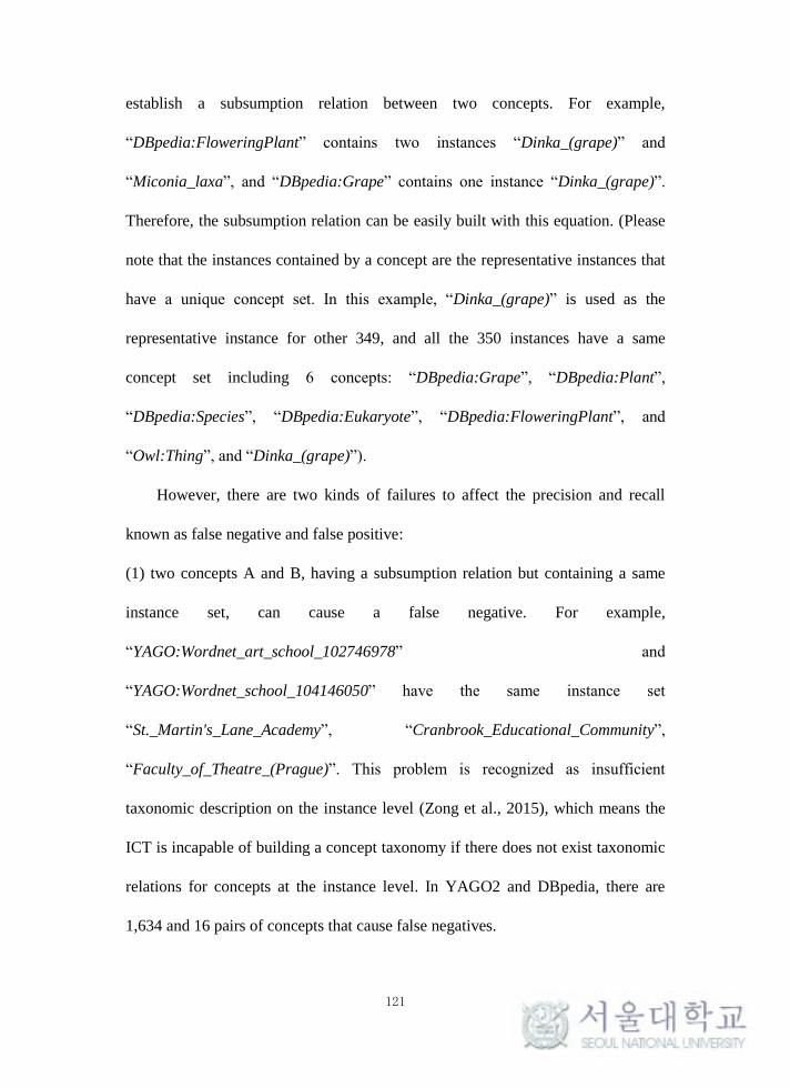
121
establish a subsumption relation between two concepts. For example,
“DBpedia:FloweringPlant” contains two instances “Dinka_(grape)” and
“Miconia_laxa”, and “DBpedia:Grape” contains one instance “Dinka_(grape)”.
Therefore, the subsumption relation can be easily built with this equation. (Please
note that the instances contained by a concept are the representative instances that
have a unique concept set. In this example, “Dinka_(grape)” is used as the
representative instance for other 349, and all the 350 instances have a same
concept set including 6 concepts: “DBpedia:Grape”, “DBpedia:Plant”,
“DBpedia:Species”, “DBpedia:Eukaryote”, “DBpedia:FloweringPlant”, and
“Owl:Thing”, and “Dinka_(grape)”).
However, there are two kinds of failures to affect the precision and recall
known as false negative and false positive:
(1) two concepts A and B, having a subsumption relation but containing a same
instance set, can cause a false negative. For example,
“YAGO:Wordnet_art_school_102746978” and
“YAGO:Wordnet_school_104146050” have the same instance set
“St._Martin's_Lane_Academy”, “Cranbrook_Educational_Community”,
“Faculty_of_Theatre_(Prague)”. This problem is recognized as insufficient
taxonomic description on the instance level (Zong et al., 2015), which means the
ICT is incapable of building a concept taxonomy if there does not exist taxonomic
relations for concepts at the instance level. In YAGO2 and DBpedia, there are
1,634 and 16 pairs of concepts that cause false negatives.
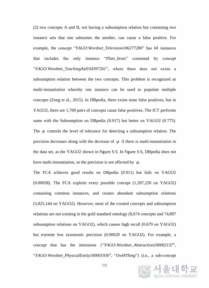
122
(2) two concepts A and B, not having a subsumption relation but containing two
instance sets that one subsumes the another, can cause a false positive. For
example, the concept “YAGO:Wordnet_Television106277280” has 68 instances
that includes the only instance “Plats_bruts” contained by concept
“YAGO:Wordnet_TeachingAid104397261”, where there does not exists a
subsumption relation between the two concepts. This problem is recognized as
multi-instantiation whereby one instance can be used to populate multiple
concepts (Zong et al., 2015). In DBpedia, there exists none false positives, but in
YAGO2, there are 1,769 pairs of concepts cause false positives. The ICT performs
same with the Subsumption on DBpedia (0.917) but better on YAGO2 (0.775).
The 𝜑 controls the level of tolerance for detecting a subsumption relation. The
precision decreases along with the decrease of 𝜑 if there is multi-instantiation in
the data set, as the YAGO2 shown in Figure 5-5. In Figure 5-5, DBpedia does not
have multi-instantiation, so the precision is not affected by 𝜑.
The FCA achieves good results on DBpedia (0.911) but fails on YAGO2
(0.00058). The FCA exploits every possible concept (1,397,220 on YAGO2)
containing common instances, and creates abundant subsumption relations
(5,825,144 on YAGO2). However, most of the created concepts and subsumption
relations are not existing in the gold standard ontology (8,674 concepts and 74,897
subsumption relations on YAGO2), which causes high recall (0.679 on YAGO2)
but extreme low taxonomic precision (0.00029 on YAGO2). For example, a
concept that has the intensions {“YAGO:Wordnet_Abstraction100002137”,
“YAGO:Wordnet_PhysicalEntity100001930”, “Owl#Thing”} (i.e., a sub-concept
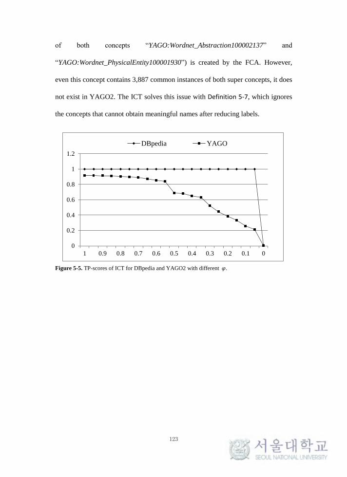
123
of both concepts “YAGO:Wordnet_Abstraction100002137” and
“YAGO:Wordnet_PhysicalEntity100001930”) is created by the FCA. However,
even this concept contains 3,887 common instances of both super concepts, it does
not exist in YAGO2. The ICT solves this issue with Definition 5-7, which ignores
the concepts that cannot obtain meaningful names after reducing labels.
Figure 5-5. TP-scores of ICT for DBpedia and YAGO2 with different 𝜑.
0
0.2
0.4
0.6
0.8
1
1.2
1 0.9 0.8 0.7 0.6 0.5 0.4 0.3 0.2 0.1 0
DBpedia YAGO
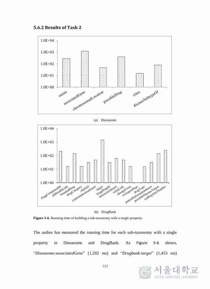
124
5.6.2 Results of Task 2
(a) Diseasome
(b) DrugBank
Figure 5-6. Running time of building a sub-taxonomy with a single property.
The author has measured the running time for each sub-taxonomy with a single
property in Diseasome and DrugBank. As Figure 5-6 shows,
“Diseasome:associatedGene” (1,202 ms) and “Drugbank:target” (1,453 ms)
1.0E+00
1.0E+01
1.0E+02
1.0E+03
1.0E+04
1.0E+00
1.0E+01
1.0E+02
1.0E+03
1.0E+04
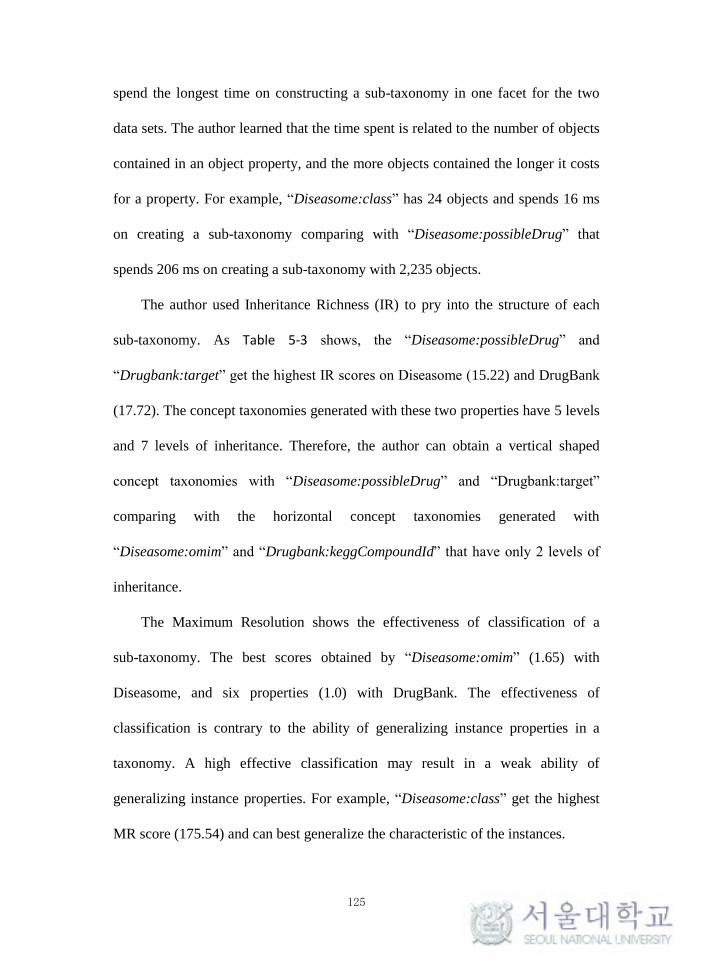
125
spend the longest time on constructing a sub-taxonomy in one facet for the two
data sets. The author learned that the time spent is related to the number of objects
contained in an object property, and the more objects contained the longer it costs
for a property. For example, “Diseasome:class” has 24 objects and spends 16 ms
on creating a sub-taxonomy comparing with “Diseasome:possibleDrug” that
spends 206 ms on creating a sub-taxonomy with 2,235 objects.
The author used Inheritance Richness (IR) to pry into the structure of each
sub-taxonomy. As Table 5-3 shows, the “Diseasome:possibleDrug” and
“Drugbank:target” get the highest IR scores on Diseasome (15.22) and DrugBank
(17.72). The concept taxonomies generated with these two properties have 5 levels
and 7 levels of inheritance. Therefore, the author can obtain a vertical shaped
concept taxonomies with “Diseasome:possibleDrug” and “Drugbank:target”
comparing with the horizontal concept taxonomies generated with
“Diseasome:omim” and “Drugbank:keggCompoundId” that have only 2 levels of
inheritance.
The Maximum Resolution shows the effectiveness of classification of a
sub-taxonomy. The best scores obtained by “Diseasome:omim” (1.65) with
Diseasome, and six properties (1.0) with DrugBank. The effectiveness of
classification is contrary to the ability of generalizing instance properties in a
taxonomy. A high effective classification may result in a weak ability of
generalizing instance properties. For example, “Diseasome:class” get the highest
MR score (175.54) and can best generalize the characteristic of the instances.
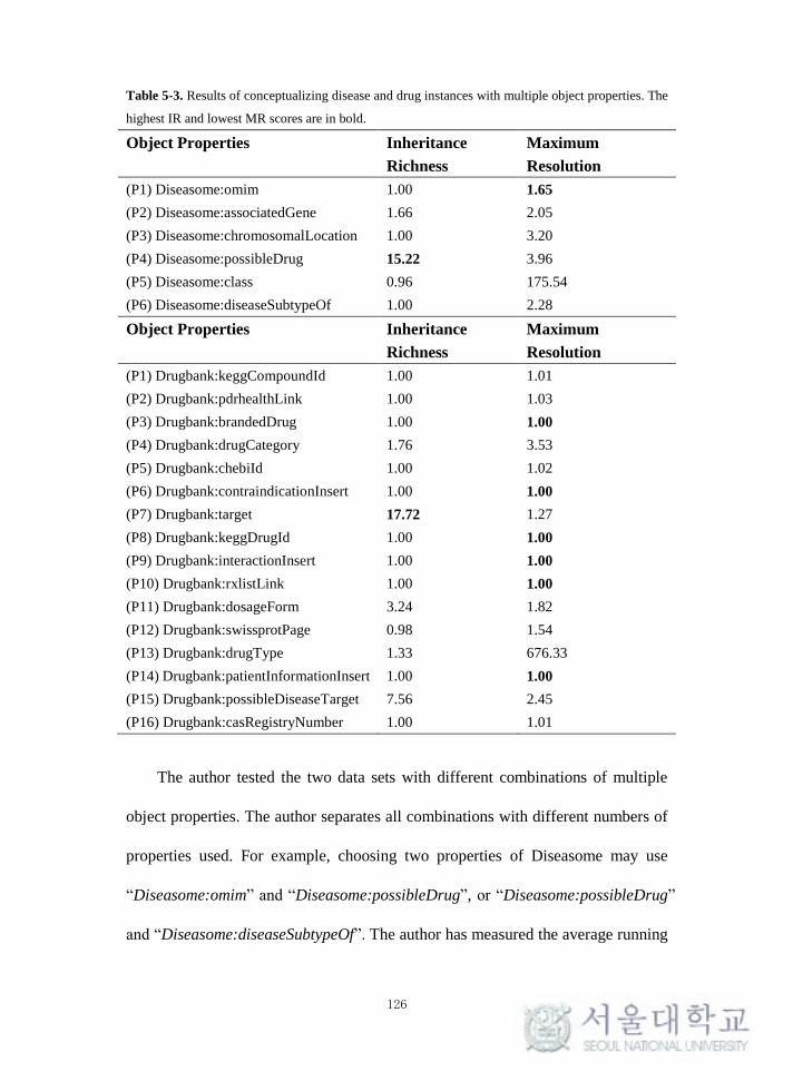
126
Table 5-3. Results of conceptualizing disease and drug instances with multiple object properties. The
highest IR and lowest MR scores are in bold.
Object Properties Inheritance
Richness
Maximum
Resolution
(P1) Diseasome:omim 1.00 1.65
(P2) Diseasome:associatedGene 1.66 2.05
(P3) Diseasome:chromosomalLocation 1.00 3.20
(P4) Diseasome:possibleDrug 15.22 3.96
(P5) Diseasome:class 0.96 175.54
(P6) Diseasome:diseaseSubtypeOf 1.00 2.28
Object Properties Inheritance
Richness
Maximum
Resolution
(P1) Drugbank:keggCompoundId 1.00 1.01
(P2) Drugbank:pdrhealthLink 1.00 1.03
(P3) Drugbank:brandedDrug 1.00 1.00
(P4) Drugbank:drugCategory 1.76 3.53
(P5) Drugbank:chebiId 1.00 1.02
(P6) Drugbank:contraindicationInsert 1.00 1.00
(P7) Drugbank:target 17.72 1.27
(P8) Drugbank:keggDrugId 1.00 1.00
(P9) Drugbank:interactionInsert 1.00 1.00
(P10) Drugbank:rxlistLink 1.00 1.00
(P11) Drugbank:dosageForm 3.24 1.82
(P12) Drugbank:swissprotPage 0.98 1.54
(P13) Drugbank:drugType 1.33 676.33
(P14) Drugbank:patientInformationInsert 1.00 1.00
(P15) Drugbank:possibleDiseaseTarget 7.56 2.45
(P16) Drugbank:casRegistryNumber 1.00 1.01
The author tested the two data sets with different combinations of multiple
object properties. The author separates all combinations with different numbers of
properties used. For example, choosing two properties of Diseasome may use
“Diseasome:omim” and “Diseasome:possibleDrug”, or “Diseasome:possibleDrug”
and “Diseasome:diseaseSubtypeOf”. The author has measured the average running
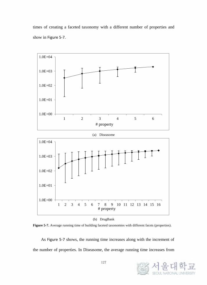
127
times of creating a faceted taxonomy with a different number of properties and
show in Figure 5-7.
(a) Diseasome
(b) DrugBank
Figure 5-7. Average running time of building faceted taxonomies with different facets (properties).
As Figure 5-7 shows, the running time increases along with the increment of
the number of properties. In Diseasome, the average running time increases from
1.0E+00
1.0E+01
1.0E+02
1.0E+03
1.0E+04
1 2 3 4 5 6
# property
1.0E+00
1.0E+01
1.0E+02
1.0E+03
1.0E+04
1 2 3 4 5 6 7 8 9 10 11 12 13 14 15 16# property
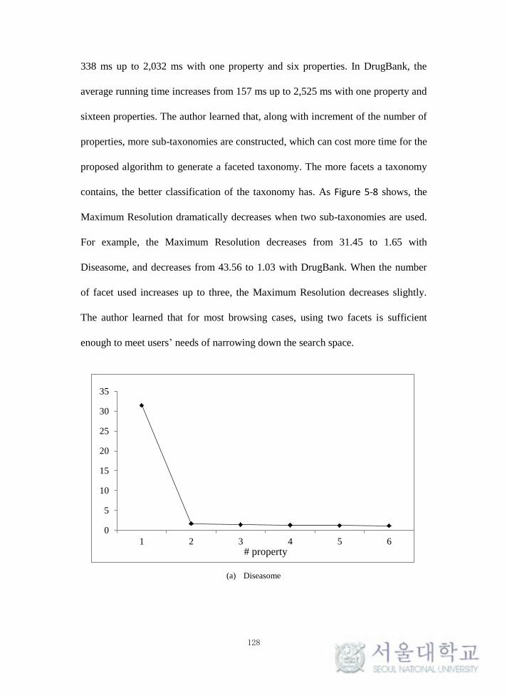
128
338 ms up to 2,032 ms with one property and six properties. In DrugBank, the
average running time increases from 157 ms up to 2,525 ms with one property and
sixteen properties. The author learned that, along with increment of the number of
properties, more sub-taxonomies are constructed, which can cost more time for the
proposed algorithm to generate a faceted taxonomy. The more facets a taxonomy
contains, the better classification of the taxonomy has. As Figure 5-8 shows, the
Maximum Resolution dramatically decreases when two sub-taxonomies are used.
For example, the Maximum Resolution decreases from 31.45 to 1.65 with
Diseasome, and decreases from 43.56 to 1.03 with DrugBank. When the number
of facet used increases up to three, the Maximum Resolution decreases slightly.
The author learned that for most browsing cases, using two facets is sufficient
enough to meet users’ needs of narrowing down the search space.
(a) Diseasome
0
5
10
15
20
25
30
35
1 2 3 4 5 6# property
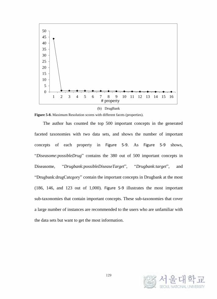
129
(b) DrugBank
Figure 5-8. Maximum Resolution scores with different facets (properties).
The author has counted the top 500 important concepts in the generated
faceted taxonomies with two data sets, and shows the number of important
concepts of each property in Figure 5-9. As Figure 5-9 shows,
“Diseasome:possibleDrug” contains the 380 out of 500 important concepts in
Diseasome, “Drugbank:possibleDiseaseTarget”, “Drugbank:target”, and
“Drugbank:drugCategory” contain the important concepts in Drugbank at the most
(186, 146, and 123 out of 1,000). Figure 5-9 illustrates the most important
sub-taxonomies that contain important concepts. These sub-taxonomies that cover
a large number of instances are recommended to the users who are unfamiliar with
the data sets but want to get the most information.
0
5
10
15
20
25
30
35
40
45
50
1 2 3 4 5 6 7 8 9 10 11 12 13 14 15 16# property
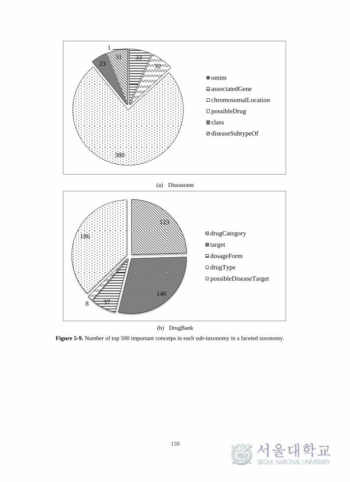
130
(a) Diseasome
(b) DrugBank
Figure 5-9. Number of top 500 important concetps in each sub-taxonomy in a faceted taxonomy.
1
33
32
380
23 31
omim
associatedGene
chromosomalLocation
possibleDrug
class
diseaseSubtypeOf
123
146
37 8
186 drugCategory
target
dosageForm
drugType
possibleDiseaseTarget
131
5.7 Discussion
The sub-taxonomies in each facet are constructed based on the concepts defined
by the author in Section 5.4.2. This definition leaves two issues to be discussed
when a faceted taxonomy is generated:
First, the concepts are removed when the concepts are unrecognizable with
reduced labeling strategy in Definition 5-7. The definition has two benefits: (1)
reduces unnecessary computations and decreases running time when the proposed
method constructs a sub-taxonomy, and (2) reduces multiple inheritance when the
concepts have multiple super concepts, and increases Taxonomic F-measure
scores. However, the concept reducing strategy used in Definition 5-7 is still
insufficient enough to prevent multiple inheritance, which the author has observed
in the first task with YAGO2 in Section 5.6.1. To remove the meaningless
concepts by judging the concept name is too simple and primitive, and the method
only considers the semantics of the intension rather than the extension of a concept.
There can be a more sophisticated method to decide the validity of a concept by
balancing both the extensions and intensions of a concept, which leaves a potential
improvement for future.
Second, the concepts are defined with the extensions (i.e., instances) and
recognized with intensions (i.e., objects of properties). The concept definition and
naming strategy the author applied has the advantages of improving efficiency and
effectiveness, but leaves a difficulty of understanding the concepts. For example in
the taxonomy in the facet “Diseasome:possibleDrug” for Diseasome in Section
5.6.2, the author found that the concept labeled as “Drug:DB00898” (Ethanol) is
132
the super concept of the concept labeled as “Drug:DB03929” (D-Serine), and it is
hard to interpret the two concepts having a “is_A” relation semantically. However,
the two concepts can be understood as having a subsumption relation in extension,
since “Drug:DB03929” can treat “Disease:2666” (Hyperekplexia and spastic
paraparesis), and “Drug:DB00898” can treat “Disease:2666”,
“Disease:372”(Epilepsy), and “Disease:2312” (Epilepsy, juvenile myoclonic,
606904). In addition, viewing from the instance level, the ancestors of a concept
are those contained by its instances in a facet. In the same example, “Disease:2666”
can be treat by the possible drugs “Drug:DB00898” and “Drug:DB03929”.
Therefore, the concepts in a sub-taxonomy can be understood easily to classify
instances and efficiently reduce the browsing space in a navigation (Sacco &
Tzitzikas, 2009). For example in a faceted search, if a user wants to find the
diseases that can be cured by “Drug:DB03929”, zooming “Drug:DB00898” (i.e.,
zoom-in point (Sacco & Tzitzikas, 2009)) into “Drug:DB03929” can reduce three
diseases into only one disease.
133
5.8 Conclusion
The increasing popularity of publishing Linked Data sets addresses an issue of
constructing concept taxonomies for those data without ontologies. Instead of
building a taxonomy to classify instances from one dimension, a faceted taxonomy
that classifies instances from multiple dimensions brings the attention of academia.
However, researches focus on utilizing a faceted taxonomy with an assumption
that those taxonomies already exist. In order to provide faceted taxonomies for
faceted navigation and search in Linked Data, this study proposed a solution of
automatic construction of faceted taxonomy based on object properties. The author
has developed a framework that extracts sub data for each facet and builds a
sub-taxonomy with an instance-based Concept Taxonomy generation algorithm
called ICT based on the concept defined by the author. The author also proposed
the strategies to materialize and refine sub-taxonomies in order to get a faceted
taxonomy. The author has proven that the proposed method can achieve
encouraging results in terms of efficiency and effectiveness with two experiments.
Finally, two issues of this study are discussed to leave further improvements in the
future work.
134
6 Future Works and Conclusion
6.1 Future Works
6.1.1 Similarity Measures for Instance-based Schema Alignment
There are diverse similarity measures for instance-based schema alignment. A
concept can be represented with a set of instances. Therefore, similarity measures
used for sets can be applied, such as Jaccard similarity and standard
information-theory measures (e.g., Pointwise Mutual Information, Log Likelihood
ratio, and Information Gain). The performances of these metrics are discussed in
(Isaac et al., 2007), which shows that the Jaccard similarity outperforms other
similarity measures. Performance of other measures, such as Dice similarity,
Minimum similarity, and Kappa similarity, however, varies depending on the link
data used (Kirsten et al., 2007). So far, there is no direct guideline in selecting a
measure for instance-based schema alignment. However, we can easily calculate
that for two concepts c1 and c2 , 𝑠𝑖𝑚𝑑𝑖𝑐𝑒(𝑐1, 𝑐2) ≤ 𝑠𝑖𝑚𝑚𝑖𝑛(𝑐1, 𝑐2) and
𝑠𝑖𝑚𝑗𝑎𝑐𝑐𝑎𝑟𝑑(𝑐1, 𝑐2) ≤ 𝑠𝑖𝑚𝑚𝑖𝑛(𝑐1, 𝑐2) . Therefore, with the same threshold for
determining equivalence, there are more equivalence alignments by using
Minimum similarity than using Dice similarity and Jaccard similarity, which causes
high recall but low precision for Minimum similarity-based method, and low recall
but high precision for Dice similarity- and Jaccard similarity-based methods. A
more detailed experiment could illustrate the performances of these similarity
metrics with different data in my future work.
135
With the Vector Space Model, a concept can be represented as a vector with the
values corresponding to the instance set of the concept. The vector values can be
weighted by term (instance) frequency measures, such as TF/IDF. Therefore,
similarity measures for vectors can be applied, such as cosine similarity. An
interesting attempt is to compare the alignments generated with the same cosine
similarity measure using the vectors with TF/IDF values and binary values (a.k.a.,
Ochiai coefficient for computing two instance sets). The cosine similarity measure
can be estimated with Radom Hyperplane in LSH. Therefore, replacing Jaccard
similarity with Cosine similarity can be a meaningful extension for our proposed
method in Section 3.
6.1.2 Ontology Evolution for Instance-based Schema Alignment
Along with the development of linked data, Ontologies representing knowledge of
the data also evolve continuously. For example, new classes are added or removed
from the original ontology along with the adding of new domain data or deleting
of old domain data. Not only instances belonging to a class could vary (add or
delete) but also relations between classes can change.
The ontology evolution affects schema alignment results, especially for
instance-based methods (Hartung, Kirsten, & Rahm, 2008; Thor, Hartung, Gross,
Kirsten, & Rahm, 2009). The author has observed the different alignment results
caused by evolution of DBpedia and YAGO2 in Section 3.6. The evolution of life
science ontologies has been discussed in (Hartung et al., 2008; Thor et al., 2009),
However, there still lacks the study of the affections in Linked Data evolution on
136
schema alignment. The future work will focus on answering three questions on
this issue: (1) how to analyze affections of ontology evolution on schema
alignment, (2) how to evaluate alignments from the perspective of ontology
evolution, and (3) how to align schemas with considering ontology evolutions
(several versions of the same ontology).
6.1.3 Combining the IUT with Structure- and Lexical-based
Methods
The author has proposed the IUT that aligns schemas based on instances.
Instance-based method is considered as a better solution for aligning schemas with
ambiguous names. However, lexical- (or linguistic) and structure-based methods
are frequently used in schema alignment. Lexical-based similarities are used in
pre-matching to select candidate matched pairs for other sophisticated matchers
(Bellahsene et al., 2011). The lexical-based methods are more efficient than
instance-based methods for classes with a huge number of instances.
Structure-based method is considered to align two classes with a more
comprehensive view. For example, Similarity Flooding (Melnik, Garcia-Molina,
& Rahm, 2002) is used to reassign similarities to matched pairs based on the
schema structure. The IUT can adapt the two kinds of methods to give a hybrid
solution for schema alignment to: (1) improve the efficiency with lexical-based
methods, and (2) improve the effectiveness with structure-based methods.
137
6.1.4 Scaling the IUT with Parallel Computations
There are two ways generally to scale schema alignment as the author introduced
in Section 2.2.2. In Chapter 4, the author scales the IUT based on decreasing
similarity computations for classes. However, there is another solution to scale
matching with parallel computations, such as MapReduce. In parallel computation
based scaling methods, matchers should be independent. In the IUT, the classes
de-queued from the class-relation multi-graph should compare all the classes
already in the virtual graph to find an appropriate position with a matcher. Even
though, similarity computations in a matcher are independent and can be
computed in parallel, it is still not sufficient enough. Matchers with the input
de-queued classes are sequenced and not independent. Therefore, MapReduce
cannot be directly adapted to the matchers in the IUT. The future work is to
change the IUT to allow using MapReduce to improve the efficiency.
6.1.5 Faceted Navigation and Search for Linked Data
The author has proposed a method to automatically generate a faceted taxonomy
based on object properties. The taxonomy generated is the foundation of realizing
faceted navigation and search. However, several issues still remain and are needed
to be further studied: (1) how to decide the object properties to generate a faceted
taxonomy that satisfies users search intension; (2) how to efficiently expand
concepts dynamically in a faceted taxonomy to provide a comprehensive view of
data sets; (3) how to apply ontology alignment method introduced in Chapter 3 to
align the faceted taxonomy with existing ontologies to improve the experience of

138
navigation and search for Linked Data consumers. The future work is to develop a
faceted navigation and search system that answers these questions addressed by
the author.
139
6.2 Conclusion
This thesis solves three issues in instance-based schema alignment in Linked Data,
(1) how to align schemas based on instances, (2) how to scale the schema
alignment, and (3) how to generate hierarchical schema structure, with three
proposed methods introduced in Chapters 3, 4, and 5.
There many types of ontologies in Linked Data, and the alignments of the
ontologies have been performed diversely in our proposed method demonstrated in
Section 3. Therefore, in the end of the thesis, the author wants to category the
features of the ontologies targeted by the proposed methods. The sufficient feature
of the targeted ontologies for the proposed method is the establishment of
“Owl:sameAs” alignments between instances.
(1) Alignment on instances (with “Owl:sameAs”)
The instance-based alignment methods measure the similarity of two concepts
with common instances. Therefore, in Linked Data, ontologies have to be aligned
with “Owl:sameAs” or other links that provide similar functions.
There are other three features would cause the better alignments for the targeted
ontologies by the proposed method than other methods, which are (1) ambiguous
or without naming, (2) rich instantiation, and (3) keen hierarchical taxonomy and
instantiation.
(1) Ambiguous naming or even without naming
The lexical-based matchers are incapable of finding mappings when schema
elements have ambiguous or obscure names, or even without names (e.g., blank
140
nodes). Therefore, ontologies with ambiguous names or without names are
suggested to be aligned with instance.
(2) Rich instances
As Section 3.5 shows, ontology alignment on the concepts with a large number of
instances works better than on those with a limited number of instances. Therefore,
the author recommends to align the ontologies with a large number of instances.
However, the author still lacks a guideline on determine a threshold for the
instance number contained by a concept. According to the study in (Isaac et al.,
2007), a threshold improves precision but hurts recall. A practical threshold should
be decided based on a user’s requirement on alignment in a real application.
(3) Keen hierarchical taxonomy and instantiation.
An ontology aligned based on instances should have a hierarchical taxonomy for
the schema. However, if this condition is not satisfied, a taxonomy can be
automatically generated with the ICT proposed in Chapter 5. According to the
experiment results in Section 3.5, three facts can affect the performance of the
alignment, which are insufficient taxonomy, multiple inheritance, and multiple
instantiation.
Sufficient taxonomy means that a concept is sufficiently classified by
multiple sub-concepts (i.e., one concept has more than one sub-concept).
Non-multiple inheritance means that a concept cannot have multiple super
concepts. Non-multiple instantiation means an instance cannot be used to populate
multiple concepts. Please note that multiple inheritance can cause multiple
instantiation but not vice versa.
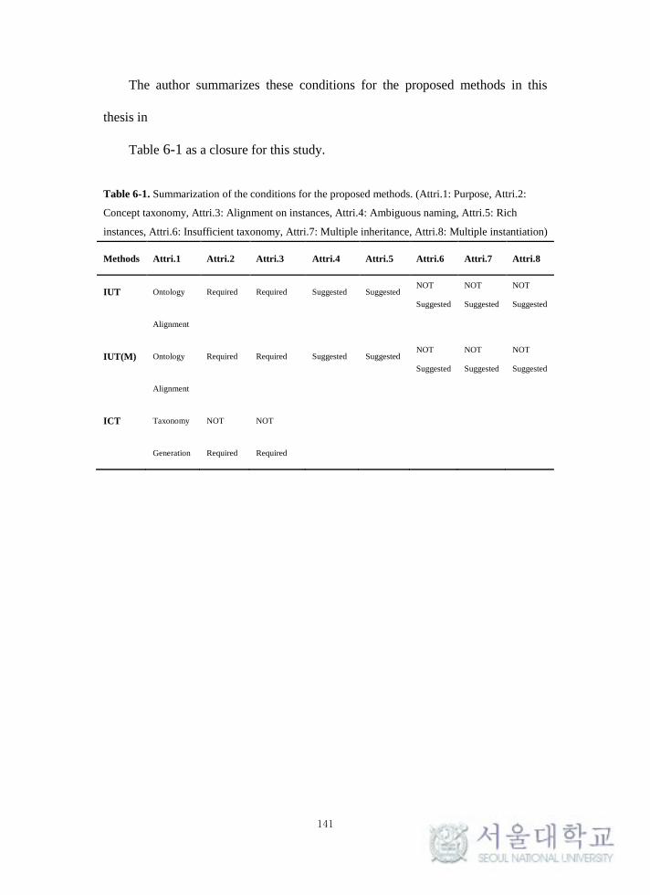
141
The author summarizes these conditions for the proposed methods in this
thesis in
Table 6-1 as a closure for this study.
Table 6-1. Summarization of the conditions for the proposed methods. (Attri.1: Purpose, Attri.2:
Concept taxonomy, Attri.3: Alignment on instances, Attri.4: Ambiguous naming, Attri.5: Rich
instances, Attri.6: Insufficient taxonomy, Attri.7: Multiple inheritance, Attri.8: Multiple instantiation)
Methods Attri.1 Attri.2 Attri.3 Attri.4 Attri.5 Attri.6 Attri.7 Attri.8
IUT Ontology
Alignment
Required Required Suggested Suggested NOT
Suggested
NOT
Suggested
NOT
Suggested
IUT(M) Ontology
Alignment
Required Required Suggested Suggested NOT
Suggested
NOT
Suggested
NOT
Suggested
ICT Taxonomy
Generation
NOT
Required
NOT
Required
142
Bibliography
2009 Campaign - Ontology Alignment Evaluation Initiative. (2009). Retrieved 10/14, 2014, from
http://oaei.ontologymatching.org/2009/
Alani, Harith, Kim, Sanghee, Millard, David E., Weal, Mark J., Hall, Wendy, Lewis, Paul H., &
Shadbolt, Nigel R. (2003). Automatic Ontology-Based Knowledge Extraction from Web
Documents. IEEE Intelligent Systems, 18(1), 14-21. doi: 10.1109/mis.2003.1179189
Arasu, Arvind, Ganti, Venkatesh, & Kaushik, Raghav. (2006). Efficient exact set-similarity joins.
Paper presented at the Proceedings of the 32nd international conference on Very large data
bases, Seoul, Korea.
Astrova, Irina. (2004). Reverse engineering of relational databases to ontologies The Semantic Web:
Research and Applications (pp. 327-341): Springer.
Batini, C., Lenzerini, M., & Navathe, S. B. (1986). A comparative analysis of methodologies for
database schema integration. ACM Comput. Surv., 18(4), 323-364. doi:
10.1145/27633.27634
Bayardo, Roberto J., Ma, Yiming, & Srikant, Ramakrishnan. (2007). Scaling up all pairs similarity
search. Paper presented at the Proceedings of the 16th international conference on World
Wide Web, Banff, Alberta, Canada.
Bechhofer, Sean, Harmelen, Frank van, Hendler, Jim, Horrocks, Ian, McGuinness, Deborah L.,
Patel-Schneider, Peter F., & Stein, Lynn Andrea. (2004). OWL Web Ontology Language
Reference. from http://www.w3.org/TR/owl-ref/
Bedini, Ivan, Matheus, Christopher, Patel-Schneider, Peter F., Boran, Aidan, & Nguyen, Benjamin.
(2011). Transforming XML Schema to OWL Using Patterns. Paper presented at the
Proceedings of the 2011 IEEE Fifth International Conference on Semantic Computing.
Bedini, Ivan, & Nguyen, Benjamin. (2007). Automatic ontology generation: State of the art. PRiSM
Laboratory Technical Report. University of Versailles.
Bellahsene, Zohra, Bonifati, Angela, & Rahm, Erhard. (2011). Schema Matching and Mapping:
Springer Publishing Company, Incorporated.
Best Practice Recipes for Publishing RDF Vocabularies.). Retrieved 10/20, 2014, from
http://www.w3.org/TR/swbp-vocab-pub/
Bilke, Alexander, & Naumann, Felix. (2005). Schema Matching Using Duplicates. Paper presented at
the Proceedings of the 21st International Conference on Data Engineering, Washington, DC,
USA.
Bizer, Christian. (2011). Evolving the web into a global data space. Paper presented at the Proceedings
of the 28th British national conference on Advances in databases, Manchester, UK.
Bizer, Christian, Heath, Tom, & Berners-Lee, Tim. (2009). Linked data-the story so far. International
journal on semantic web and information systems, 5(3), 1-22.
BLOOMS. 2013/04/18). from http://wiki.knoesis.org/index.php/BLOOMS
143
Blum, Daniel, & Cohen, Sara. (2010). Generating RDF for application testing. Paper presented at the
9th International Semantic Web Conference ISWC 2010.
Brewster, Christopher, & Wilks, Yorick. (2004). Ontologies, Taxonomies, Thesauri Learning from
Texts. Paper presented at the The Keyword Project: Unlocking Content through
Computational Linguistics.
http://www.kcl.ac.uk/humanities/cch/ake/final/content/pubs/pub01.html
Broder, Andrei Z., Glassman, Steven C., Manasse, Mark S., & Zweig, Geoffrey. (1997). Syntactic
clustering of the Web. Comput. Netw. ISDN Syst., 29(8-13), 1157-1166. doi:
10.1016/s0169-7552(97)00031-7
Carroll, Jeremy, Herman, Ivan, & Patel-Schneider, Peter F. (2012). OWL 2 Web Ontology Language
RDF-Based Semantics (Second Edition). from
http://www.w3.org/TR/owl2-rdf-based-semantics/#Content_of_Ontologies_.28Informative
.29
Cerbah, Farid. (2008). Mining the Content of Relational Databases to Learn Ontologies with Deeper
Taxonomies. Paper presented at the Proceedings of the 2008 IEEE/WIC/ACM International
Conference on Web Intelligence and Intelligent Agent Technology - Volume 01.
Chaudhuri, Surajit, Ganti, Venkatesh, & Kaushik, Raghav. (2006). A Primitive Operator for Similarity
Joins in Data Cleaning. Paper presented at the Proceedings of the 22nd International
Conference on Data Engineering.
Cimiano, Philipp, Hotho, Andreas, & Staab, Steffen. (2005). Learning concept hierarchies from text
corpora using formal concept analysis. J. Artif. Int. Res., 24(1), 305-339.
Class (philosophy). 2014/02/19). Retrieved 10/17, 2014, from
http://en.wikipedia.org/wiki/Class_(philosophy)
Colibri-Java.). Retrieved 04.29, 2015, from http://code.google.com/p/colibri-java/
Cruz, Isabel F., Antonelli, Flavio Palandri, & Stroe, Cosmin. (2009). AgreementMaker: efficient
matching for large real-world schemas and ontologies. Proc. VLDB Endow., 2(2),
1586-1589. doi: 10.14778/1687553.1687598
Czarnecki, K., & Helsen, S. (2006). Feature-based survey of model transformation approaches. IBM
Syst. J., 45(3), 621-645. doi: 10.1147/sj.453.0621
Dasgupta, Sourish, Dinakarpandian, Deendayal, & Lee, Yugyung. (2007). A Panoramic Approach to
Integrated Evaluation of Ontologies in the Semantic Web. Paper presented at the EON.
David, Jérôme, Guillet, Fabrice, & Briand, Henri. (2006). Matching directories and OWL ontologies
with AROMA. Paper presented at the Proceedings of the 15th ACM international conference
on Information and knowledge management, Arlington, Virginia, USA.
DBpedia. 2014). Retrieved 10/14, 2014, from http://wiki.dbpedia.org/About
Dean, Jeffrey, & Ghemawat, Sanjay. (2008). MapReduce: simplified data processing on large clusters.
Commun. ACM, 51(1), 107-113. doi: 10.1145/1327452.1327492
144
Dellschaft, Klaas, & Staab, Steffen. (2006). On how to perform a gold standard based evaluation of
ontology learning. Paper presented at the Proceedings of the 5th international conference on
The Semantic Web, Athens, GA.
Ding, Li, DiFranzo, Dominic, Graves, Alvaro, Michaelis, James R., Li, Xian, McGuinness, Deborah L.,
& Hendler, James A. (2010). TWC data-gov corpus: incrementally generating linked
government data from data.gov. Paper presented at the Proceedings of the 19th international
conference on World wide web, Raleigh, North Carolina, USA.
Diseasome.). Retrieved 10/14, 2014, from http://diseasome.eu/
Doan, AnHai, & Halevy, Alon Y. (2005). Semantic-integration research in the database community.
AI Mag., 26(1), 83-94.
Doan, AnHai, Madhavan, Jayant, Domingos, Pedro, & Halevy, Alon. (2004). Ontology Matching: A
Machine Learning Approach. In S. Staab & R. Studer (Eds.), Handbook on Ontologies (pp.
385-403): Springer Berlin Heidelberg.
Downloads - Dbpedia.). Retrieved 10/14, 2014, from http://downloads.dbpedia.org/
Downloads - YAGO2.). Retrieved 10/14, 2014, from
http://www.mpi-inf.mpg.de/departments/databases-and-information-systems/research/yago
-naga/yago/downloads/
DrugBank.). Retrieved 10/15, 2014, from http://www.drugbank.ca/
Drymonas, Euthymios, Zervanou, Kalliopi, & Petrakis, Euripides G. M. (2010). Unsupervised
ontology acquisition from plain texts: the OntoGain system. Paper presented at the
Proceedings of the Natural language processing and information systems, and 15th
international conference on Applications of natural language to information systems, Cardiff,
UK.
Duan, Songyun, Fokoue, Achille, Hassanzadeh, Oktie, Kementsietsidis, Anastasios, Srinivas, Kavitha,
& Ward, Michael J. (2012). Instance-Based matching of large ontologies using
locality-sensitive hashing. Paper presented at the Proceedings of the 11th International
Conference on The Semantic Web - Volume Part I, Boston, MA.
Eda, Takeharu, Yoshikawa, Masatoshi, Uchiyama, Toshio, & Uchiyama, Tadasu. (2009). The
Effectiveness of Latent Semantic Analysis for Building Up a Bottom-up Taxonomy from
Folksonomy Tags. World Wide Web, 12(4), 421-440. doi: 10.1007/s11280-009-0069-1
Engmann, Daniel, & Massmann, Sabine. (2007). Instance Matching with COMA+.
Erling, Orri, & Mikhailov, Ivan. (2009). Faceted Views over Large-Scale Linked Data. Paper
presented at the LDOW.
Euzenat, Jérôme, & Shvaiko, Pavel. (2007). Ontology Matching: Springer-Verlag New York, Inc.
Ferdinand, Matthias, Zirpins, Christian, & Trastour, David. (2004). Lifting XML Schema to OWL. In
N. Koch, P. Fraternali & M. Wirsing (Eds.), Web Engineering (Vol. 3140, pp. 354-358):
Springer Berlin Heidelberg.
Freckleton, Ryan E. (2013). Scaling Ontology Alignment. University of Colorado Colorado Springs.
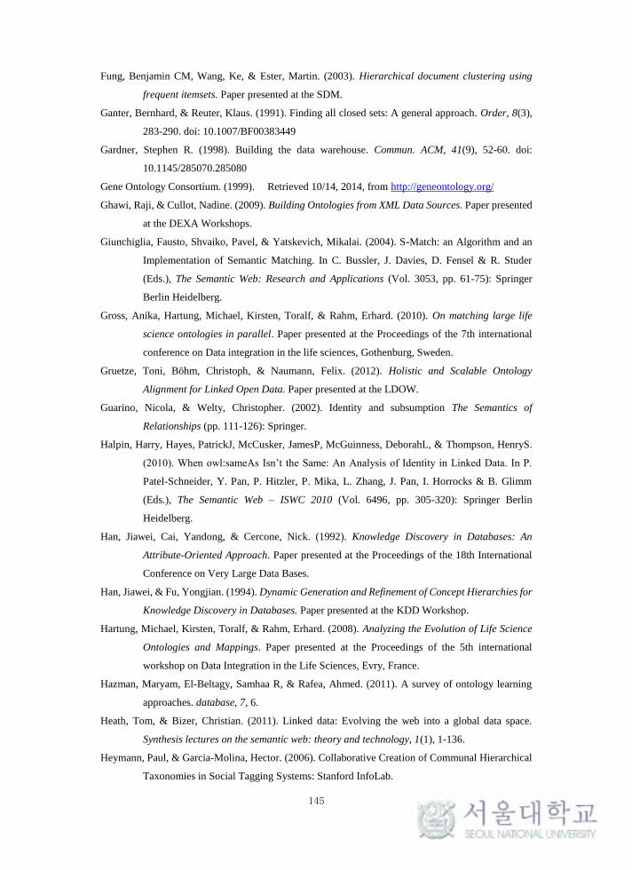
145
Fung, Benjamin CM, Wang, Ke, & Ester, Martin. (2003). Hierarchical document clustering using
frequent itemsets. Paper presented at the SDM.
Ganter, Bernhard, & Reuter, Klaus. (1991). Finding all closed sets: A general approach. Order, 8(3),
283-290. doi: 10.1007/BF00383449
Gardner, Stephen R. (1998). Building the data warehouse. Commun. ACM, 41(9), 52-60. doi:
10.1145/285070.285080
Gene Ontology Consortium. (1999). Retrieved 10/14, 2014, from http://geneontology.org/
Ghawi, Raji, & Cullot, Nadine. (2009). Building Ontologies from XML Data Sources. Paper presented
at the DEXA Workshops.
Giunchiglia, Fausto, Shvaiko, Pavel, & Yatskevich, Mikalai. (2004). S-Match: an Algorithm and an
Implementation of Semantic Matching. In C. Bussler, J. Davies, D. Fensel & R. Studer
(Eds.), The Semantic Web: Research and Applications (Vol. 3053, pp. 61-75): Springer
Berlin Heidelberg.
Gross, Anika, Hartung, Michael, Kirsten, Toralf, & Rahm, Erhard. (2010). On matching large life
science ontologies in parallel. Paper presented at the Proceedings of the 7th international
conference on Data integration in the life sciences, Gothenburg, Sweden.
Gruetze, Toni, Böhm, Christoph, & Naumann, Felix. (2012). Holistic and Scalable Ontology
Alignment for Linked Open Data. Paper presented at the LDOW.
Guarino, Nicola, & Welty, Christopher. (2002). Identity and subsumption The Semantics of
Relationships (pp. 111-126): Springer.
Halpin, Harry, Hayes, PatrickJ, McCusker, JamesP, McGuinness, DeborahL, & Thompson, HenryS.
(2010). When owl:sameAs Isn’t the Same: An Analysis of Identity in Linked Data. In P.
Patel-Schneider, Y. Pan, P. Hitzler, P. Mika, L. Zhang, J. Pan, I. Horrocks & B. Glimm
(Eds.), The Semantic Web – ISWC 2010 (Vol. 6496, pp. 305-320): Springer Berlin
Heidelberg.
Han, Jiawei, Cai, Yandong, & Cercone, Nick. (1992). Knowledge Discovery in Databases: An
Attribute-Oriented Approach. Paper presented at the Proceedings of the 18th International
Conference on Very Large Data Bases.
Han, Jiawei, & Fu, Yongjian. (1994). Dynamic Generation and Refinement of Concept Hierarchies for
Knowledge Discovery in Databases. Paper presented at the KDD Workshop.
Hartung, Michael, Kirsten, Toralf, & Rahm, Erhard. (2008). Analyzing the Evolution of Life Science
Ontologies and Mappings. Paper presented at the Proceedings of the 5th international
workshop on Data Integration in the Life Sciences, Evry, France.
Hazman, Maryam, El-Beltagy, Samhaa R, & Rafea, Ahmed. (2011). A survey of ontology learning
approaches. database, 7, 6.
Heath, Tom, & Bizer, Christian. (2011). Linked data: Evolving the web into a global data space.
Synthesis lectures on the semantic web: theory and technology, 1(1), 1-136.
Heymann, Paul, & Garcia-Molina, Hector. (2006). Collaborative Creation of Communal Hierarchical
Taxonomies in Social Tagging Systems: Stanford InfoLab.
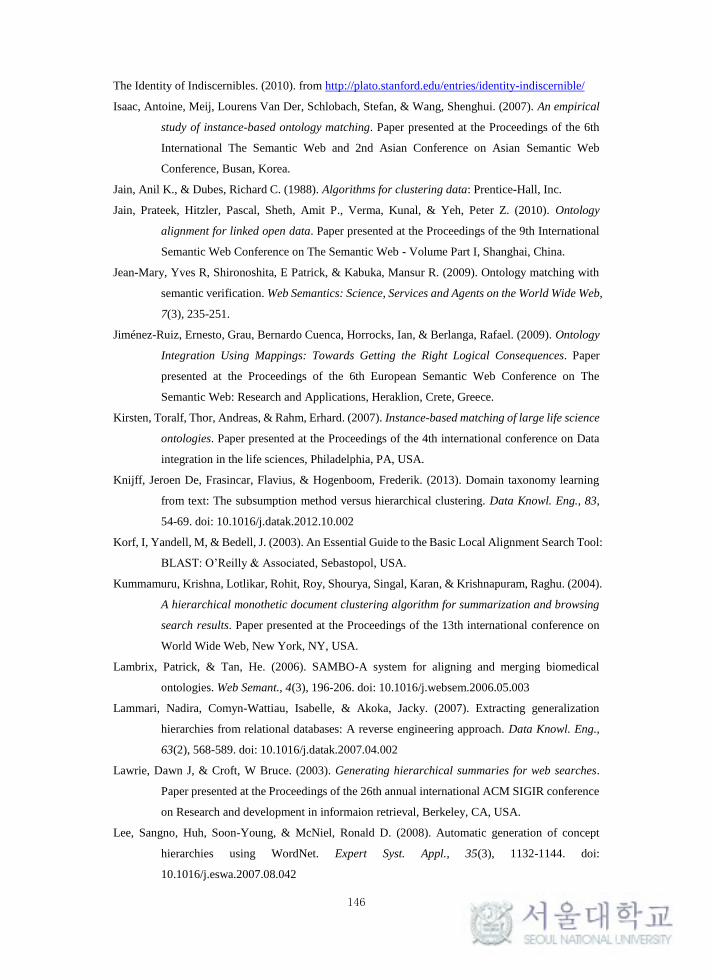
146
The Identity of Indiscernibles. (2010). from http://plato.stanford.edu/entries/identity-indiscernible/
Isaac, Antoine, Meij, Lourens Van Der, Schlobach, Stefan, & Wang, Shenghui. (2007). An empirical
study of instance-based ontology matching. Paper presented at the Proceedings of the 6th
International The Semantic Web and 2nd Asian Conference on Asian Semantic Web
Conference, Busan, Korea.
Jain, Anil K., & Dubes, Richard C. (1988). Algorithms for clustering data: Prentice-Hall, Inc.
Jain, Prateek, Hitzler, Pascal, Sheth, Amit P., Verma, Kunal, & Yeh, Peter Z. (2010). Ontology
alignment for linked open data. Paper presented at the Proceedings of the 9th International
Semantic Web Conference on The Semantic Web - Volume Part I, Shanghai, China.
Jean-Mary, Yves R, Shironoshita, E Patrick, & Kabuka, Mansur R. (2009). Ontology matching with
semantic verification. Web Semantics: Science, Services and Agents on the World Wide Web,
7(3), 235-251.
Jiménez-Ruiz, Ernesto, Grau, Bernardo Cuenca, Horrocks, Ian, & Berlanga, Rafael. (2009). Ontology
Integration Using Mappings: Towards Getting the Right Logical Consequences. Paper
presented at the Proceedings of the 6th European Semantic Web Conference on The
Semantic Web: Research and Applications, Heraklion, Crete, Greece.
Kirsten, Toralf, Thor, Andreas, & Rahm, Erhard. (2007). Instance-based matching of large life science
ontologies. Paper presented at the Proceedings of the 4th international conference on Data
integration in the life sciences, Philadelphia, PA, USA.
Knijff, Jeroen De, Frasincar, Flavius, & Hogenboom, Frederik. (2013). Domain taxonomy learning
from text: The subsumption method versus hierarchical clustering. Data Knowl. Eng., 83,
54-69. doi: 10.1016/j.datak.2012.10.002
Korf, I, Yandell, M, & Bedell, J. (2003). An Essential Guide to the Basic Local Alignment Search Tool:
BLAST: O’Reilly & Associated, Sebastopol, USA.
Kummamuru, Krishna, Lotlikar, Rohit, Roy, Shourya, Singal, Karan, & Krishnapuram, Raghu. (2004).
A hierarchical monothetic document clustering algorithm for summarization and browsing
search results. Paper presented at the Proceedings of the 13th international conference on
World Wide Web, New York, NY, USA.
Lambrix, Patrick, & Tan, He. (2006). SAMBO-A system for aligning and merging biomedical
ontologies. Web Semant., 4(3), 196-206. doi: 10.1016/j.websem.2006.05.003
Lammari, Nadira, Comyn-Wattiau, Isabelle, & Akoka, Jacky. (2007). Extracting generalization
hierarchies from relational databases: A reverse engineering approach. Data Knowl. Eng.,
63(2), 568-589. doi: 10.1016/j.datak.2007.04.002
Lawrie, Dawn J, & Croft, W Bruce. (2003). Generating hierarchical summaries for web searches.
Paper presented at the Proceedings of the 26th annual international ACM SIGIR conference
on Research and development in informaion retrieval, Berkeley, CA, USA.
Lee, Sangno, Huh, Soon-Young, & McNiel, Ronald D. (2008). Automatic generation of concept
hierarchies using WordNet. Expert Syst. Appl., 35(3), 1132-1144. doi:
10.1016/j.eswa.2007.08.042
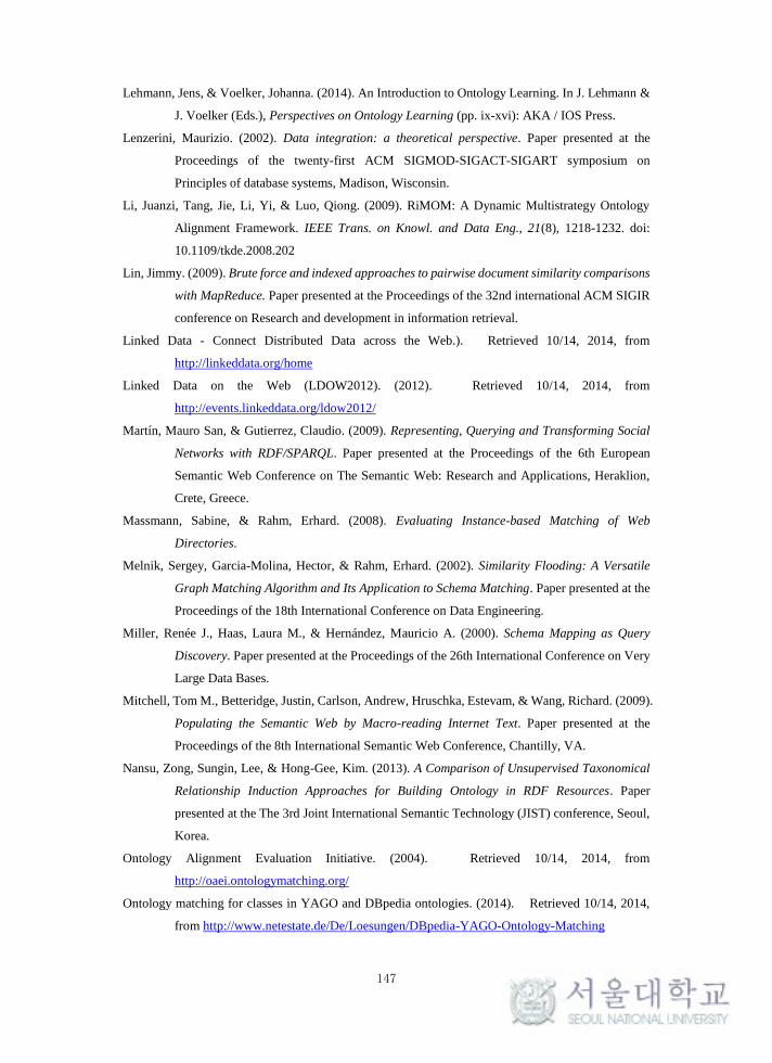
147
Lehmann, Jens, & Voelker, Johanna. (2014). An Introduction to Ontology Learning. In J. Lehmann &
J. Voelker (Eds.), Perspectives on Ontology Learning (pp. ix-xvi): AKA / IOS Press.
Lenzerini, Maurizio. (2002). Data integration: a theoretical perspective. Paper presented at the
Proceedings of the twenty-first ACM SIGMOD-SIGACT-SIGART symposium on
Principles of database systems, Madison, Wisconsin.
Li, Juanzi, Tang, Jie, Li, Yi, & Luo, Qiong. (2009). RiMOM: A Dynamic Multistrategy Ontology
Alignment Framework. IEEE Trans. on Knowl. and Data Eng., 21(8), 1218-1232. doi:
10.1109/tkde.2008.202
Lin, Jimmy. (2009). Brute force and indexed approaches to pairwise document similarity comparisons
with MapReduce. Paper presented at the Proceedings of the 32nd international ACM SIGIR
conference on Research and development in information retrieval.
Linked Data - Connect Distributed Data across the Web.). Retrieved 10/14, 2014, from
http://linkeddata.org/home
Linked Data on the Web (LDOW2012). (2012). Retrieved 10/14, 2014, from
http://events.linkeddata.org/ldow2012/
Martín, Mauro San, & Gutierrez, Claudio. (2009). Representing, Querying and Transforming Social
Networks with RDF/SPARQL. Paper presented at the Proceedings of the 6th European
Semantic Web Conference on The Semantic Web: Research and Applications, Heraklion,
Crete, Greece.
Massmann, Sabine, & Rahm, Erhard. (2008). Evaluating Instance-based Matching of Web
Directories.
Melnik, Sergey, Garcia-Molina, Hector, & Rahm, Erhard. (2002). Similarity Flooding: A Versatile
Graph Matching Algorithm and Its Application to Schema Matching. Paper presented at the
Proceedings of the 18th International Conference on Data Engineering.
Miller, Renée J., Haas, Laura M., & Hernández, Mauricio A. (2000). Schema Mapping as Query
Discovery. Paper presented at the Proceedings of the 26th International Conference on Very
Large Data Bases.
Mitchell, Tom M., Betteridge, Justin, Carlson, Andrew, Hruschka, Estevam, & Wang, Richard. (2009).
Populating the Semantic Web by Macro-reading Internet Text. Paper presented at the
Proceedings of the 8th International Semantic Web Conference, Chantilly, VA.
Nansu, Zong, Sungin, Lee, & Hong-Gee, Kim. (2013). A Comparison of Unsupervised Taxonomical
Relationship Induction Approaches for Building Ontology in RDF Resources. Paper
presented at the The 3rd Joint International Semantic Technology (JIST) conference, Seoul,
Korea.
Ontology Alignment Evaluation Initiative. (2004). Retrieved 10/14, 2014, from
http://oaei.ontologymatching.org/
Ontology matching for classes in YAGO and DBpedia ontologies. (2014). Retrieved 10/14, 2014,
from http://www.netestate.de/De/Loesungen/DBpedia-YAGO-Ontology-Matching
148
Oren, Eyal, Delbru, Renaud, & Decker, Stefan. (2006). Extending faceted navigation for RDF data.
Paper presented at the Proceedings of the 5th international conference on The Semantic Web,
Athens, GA.
OWL.). Retrieved 10/20, 2014, from http://www.w3.org/2002/07/owl
Parundekar, Rahul, Knoblock, Craig A., & Ambite, José Luis. (2010). Linking and building ontologies
of linked data. Paper presented at the Proceedings of the 9th International Semantic Web
Conference on The Semantic Web - Volume Part I, Shanghai, China.
Paukkeri, Mari-Sanna, García-Plaza, Alberto Pérez, Fresno, Víctor, Unanue, Raquel Martínez, &
Honkela, Timo. (2012). Learning a taxonomy from a set of text documents. Appl. Soft
Comput., 12(3), 1138-1148. doi: 10.1016/j.asoc.2011.11.009
Piateski, Gregory, & Frawley, William. (1991). Knowledge Discovery in Databases: MIT Press.
Pivk, Aleksander. (2006). Thesis: automatic ontology generation from web tabular structures. AI
Commun., 19(1), 83-85.
Rahm, Erhard, & Bernstein, Philip A. (2001). A survey of approaches to automatic schema matching.
The VLDB Journal, 10(4), 334-350. doi: 10.1007/s007780100057
Rajaraman, Anand, & Ullman, Jeffrey David. (2011). Mining of Massive Datasets: Cambridge
University Press.
RDF Schema.). Retrieved 10/20, 2014, from http://www.w3.org/2000/01/rdf-schema
Repository overview - Linked Life Data. (2009). Retrieved 10/14, 2014, from
http://linkedlifedata.com/sources.html
Resource Description Framework (RDF).). Retrieved 10/17, 2014, from http://www.w3.org/RDF/
Resource Description Framework (RDF) Model and Syntax Specification. (1999). Retrieved 10/19,
2014, from http://www.w3.org/TR/PR-rdf-syntax/
Resource Description Framework (Wiki).). Retrieved 10/19, 2014, from
http://en.wikipedia.org/wiki/Resource_Description_Framework
Rodriguez-Castro, Bene, Glaser, Hugh, & Carr, Leslie. (2010). How to reuse a faceted classification
and put it on the semantic web. Paper presented at the Proceedings of the 9th international
semantic web conference on The semantic web - Volume Part I, Shanghai, China.
Sacco, Giovanni Maria, & Tzitzikas, Yannis. (2009). Dynamic Taxonomies and Faceted Search:
Theory, Practice, and Experience: Springer Publishing Company, Incorporated.
Sahoo, Satya S, Halb, Wolfgang, Hellmann, Sebastian, Idehen, Kingsley, Thibodeau Jr, Ted, Auer,
Sören, . . . Ezzat, Ahmed. (2009). A survey of current approaches for mapping of relational
databases to rdf. W3C RDB2RDF Incubator Group Report.
Sanderson, Mark, & Croft, Bruce. (1999). Deriving concept hierarchies from text. Paper presented at
the Proceedings of the 22nd annual international ACM SIGIR conference on Research and
development in information retrieval, Berkeley, California, USA.
Santoso, Heru Agus, Haw, Su-Cheng, & Abdul-Mehdi, Ziyad T. (2011). Ontology extraction from
relational database: Concept hierarchy as background knowledge. Knowledge-Based
Systems, 24(3), 457-464.
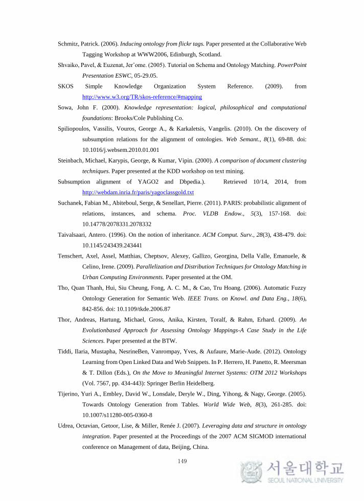
149
Schmitz, Patrick. (2006). Inducing ontology from flickr tags. Paper presented at the Collaborative Web
Tagging Workshop at WWW2006, Edinburgh, Scotland.
Shvaiko, Pavel, & Euzenat, Jerˆome. (2005). Tutorial on Schema and Ontology Matching. PowerPoint
Presentation ESWC, 05-29.05.
SKOS Simple Knowledge Organization System Reference. (2009). from
http://www.w3.org/TR/skos-reference/#mapping
Sowa, John F. (2000). Knowledge representation: logical, philosophical and computational
foundations: Brooks/Cole Publishing Co.
Spiliopoulos, Vassilis, Vouros, George A., & Karkaletsis, Vangelis. (2010). On the discovery of
subsumption relations for the alignment of ontologies. Web Semant., 8(1), 69-88. doi:
10.1016/j.websem.2010.01.001
Steinbach, Michael, Karypis, George, & Kumar, Vipin. (2000). A comparison of document clustering
techniques. Paper presented at the KDD workshop on text mining.
Subsumption alignment of YAGO2 and Dbpedia.). Retrieved 10/14, 2014, from
http://webdam.inria.fr/paris/yagoclassgold.txt
Suchanek, Fabian M., Abiteboul, Serge, & Senellart, Pierre. (2011). PARIS: probabilistic alignment of
relations, instances, and schema. Proc. VLDB Endow., 5(3), 157-168. doi:
10.14778/2078331.2078332
Taivalsaari, Antero. (1996). On the notion of inheritance. ACM Comput. Surv., 28(3), 438-479. doi:
10.1145/243439.243441
Tenschert, Axel, Assel, Matthias, Cheptsov, Alexey, Gallizo, Georgina, Della Valle, Emanuele, &
Celino, Irene. (2009). Parallelization and Distribution Techniques for Ontology Matching in
Urban Computing Environments. Paper presented at the OM.
Tho, Quan Thanh, Hui, Siu Cheung, Fong, A. C. M., & Cao, Tru Hoang. (2006). Automatic Fuzzy
Ontology Generation for Semantic Web. IEEE Trans. on Knowl. and Data Eng., 18(6),
842-856. doi: 10.1109/tkde.2006.87
Thor, Andreas, Hartung, Michael, Gross, Anika, Kirsten, Toralf, & Rahm, Erhard. (2009). An
Evolutionbased Approach for Assessing Ontology Mappings-A Case Study in the Life
Sciences. Paper presented at the BTW.
Tiddi, Ilaria, Mustapha, NesrineBen, Vanrompay, Yves, & Aufaure, Marie-Aude. (2012). Ontology
Learning from Open Linked Data and Web Snippets. In P. Herrero, H. Panetto, R. Meersman
& T. Dillon (Eds.), On the Move to Meaningful Internet Systems: OTM 2012 Workshops
(Vol. 7567, pp. 434-443): Springer Berlin Heidelberg.
Tijerino, Yuri A., Embley, David W., Lonsdale, Deryle W., Ding, Yihong, & Nagy, George. (2005).
Towards Ontology Generation from Tables. World Wide Web, 8(3), 261-285. doi:
10.1007/s11280-005-0360-8
Udrea, Octavian, Getoor, Lise, & Miller, Renée J. (2007). Leveraging data and structure in ontology
integration. Paper presented at the Proceedings of the 2007 ACM SIGMOD international
conference on Management of data, Beijing, China.
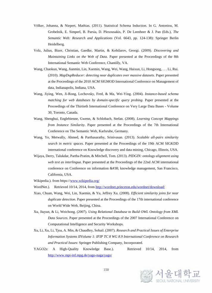
150
Völker, Johanna, & Niepert, Mathias. (2011). Statistical Schema Induction. In G. Antoniou, M.
Grobelnik, E. Simperl, B. Parsia, D. Plexousakis, P. De Leenheer & J. Pan (Eds.), The
Semantic Web: Research and Applications (Vol. 6643, pp. 124-138): Springer Berlin
Heidelberg.
Volz, Julius, Bizer, Christian, Gaedke, Martin, & Kobilarov, Georgi. (2009). Discovering and
Maintaining Links on the Web of Data. Paper presented at the Proceedings of the 8th
International Semantic Web Conference, Chantilly, VA.
Wang, Chaokun, Wang, Jianmin, Lin, Xuemin, Wang, Wei, Wang, Haixun, Li, Hongsong, . . . Li, Rui.
(2010). MapDupReducer: detecting near duplicates over massive datasets. Paper presented
at the Proceedings of the 2010 ACM SIGMOD International Conference on Management of
data, Indianapolis, Indiana, USA.
Wang, Jiying, Wen, Ji-Rong, Lochovsky, Fred, & Ma, Wei-Ying. (2004). Instance-based schema
matching for web databases by domain-specific query probing. Paper presented at the
Proceedings of the Thirtieth International Conference on Very Large Data Bases - Volume
30, Toronto, Canada.
Wang, Shenghui, Englebienne, Gwenn, & Schlobach, Stefan. (2008). Learning Concept Mappings
from Instance Similarity. Paper presented at the Proceedings of the 7th International
Conference on The Semantic Web, Karlsruhe, Germany.
Wang, Ye, Metwally, Ahmed, & Parthasarathy, Srinivasan. (2013). Scalable all-pairs similarity
search in metric spaces. Paper presented at the Proceedings of the 19th ACM SIGKDD
international conference on Knowledge discovery and data mining, Chicago, Illinois, USA.
Wijaya, Derry, Talukdar, Partha Pratim, & Mitchell, Tom. (2013). PIDGIN: ontology alignment using
web text as interlingua. Paper presented at the Proceedings of the 22nd ACM international
conference on Conference on information & knowledge management, San Francisco,
California, USA.
Wikipedia.). from https://www.wikipedia.org/
WordNet.). Retrieved 10/14, 2014, from http://wordnet.princeton.edu/wordnet/download/
Xiao, Chuan, Wang, Wei, Lin, Xuemin, & Yu, Jeffrey Xu. (2008). Efficient similarity joins for near
duplicate detection. Paper presented at the Proceedings of the 17th international conference
on World Wide Web, Beijing, China.
Xu, Jiuyun, & Li, Weichong. (2007). Using Relational Database to Build OWL Ontology from XML
Data Sources. Paper presented at the Proceedings of the 2007 International Conference on
Computational Intelligence and Security Workshops.
Xu, Li, Xu, Li, Tjoa, A. Min, & Chaudhry, Sohail. (2007). Research and Practical Issues of Enterprise
Information Systems IIVolume 1: IFIP TC 8 WG 8.9 International Conference on Research
and Practical Issues: Springer Publishing Company, Incorporated.
YAGO2s: A High-Quality Knowledge Base.). Retrieved 10/14, 2014, from
http://www.mpi-inf.mpg.de/yago-naga/yago/
151
Zhang, Hang, Hu, Wei, & Qu, Yuzhong. (2012). Constructing virtual documents for ontology
matching using mapreduce. Paper presented at the Proceedings of the 2011 joint
international conference on The Semantic Web, Hangzhou, China.
Zheng, Hai-Tao, Borchert, Charles, & Kim, Hong-Gee. (2008). A Concept-Driven Automatic
Ontology Generation Approach for Conceptualization of Document Corpora. Paper
presented at the Proceedings of the 2008 IEEE/WIC/ACM International Conference on Web
Intelligence and Intelligent Agent Technology - Volume 01.
Zhu, Man, Gao, Zhiqiang, Pan, Jeff Z., Zhao, Yuting, Xu, Ying, & Quan, Zhibin. (2015). TBox
learning from incomplete data by inference in BelNet+. Knowledge-Based Systems, 75(0),
30-40. doi: http://dx.doi.org/10.1016/j.knosys.2014.11.004
Zong, Nansu, Nam, Sejin, Eom, Jae-Hong, Ahn, Jinhyun, Joe, Hyunwhan, & Kim, Hong-Gee. (2015).
Aligning ontologies with subsumption and equivalence relations in Linked Data.
Knowledge-Based Systems, 76(0), 30-41. doi:
http://dx.doi.org/10.1016/j.knosys.2014.11.022

152
초록
링크드 데이터에 대한 인스턴스
기반 온톨로지 매핑
웹이 발전함에 따라 사용자는 복잡한 질의에 대해서도 웹이 알기 쉽게
정보를 찾아주길 원하고 있다. 이를 위해서는 다양한 형태의 데이터를
공유, 교환 그리고 통합하는 수단이 필요하다. 하지만, 웹에 공개된
데이터들은 관련된 데이터들과 통합하기 위한 의미정보가 결여된 경우가
많다. RDF 와 링크드 데이터는 잘 정의된 관계를 사용해서 데이터를
연결함으로써 의미정보를 표현하기 위해 제안됐다. RDF 와 링크드
데이터가 널리 사용됨에 따라 분절된 데이터들이 가지고 있는 의미정보를
제공하기 위한 온톨로지 매핑 기술이 주목을 받고 있다. 하지만, 링크드
데이터에 대한 온톨로지 매핑 기술은 스키마 보다는 인스턴스 레벨에
초점을 맞춰왔다. 링크드 데이터에 대한 옽톨로지 매핑은 인스턴스
레벨의 매핑이 존재하는 경우에만 스키마 레벨 매핑이 가능하다. 링크드
데이터는 인스턴스 기반의 스키마 매핑 기술을 적용하기에 적합한
데이터이다. 특히 모호한 이름을 가지고 있는 클래스 간의 매핑을 할 때
유용하다.
153
본 논문에서는 링크드 데이터에 대한 인스턴스 기반 스키마 매핑에 관한
세 가지 문제를 다뤘다. (1) 인스턴스 기반 스키마 매핑 (2) 대용량 링크드
데이터에 적용 가능하도록 알고리즘 개선 (3) 계층구조 생성
(1) 첫 번째 문제에 대해, 본 논문에서는 인스턴스 기반 스키마 매핑
알고리즘(IUT)을 제안했다. IUT 는 두 개의 대상 온톨로지에 있는
클래스들을 통합하여 하나의 계층구조를 생성한다. 이를 위해
인스턴스-클래스 매트릭스를 구축하고 인스턴스를 얼마나 공유하는지에
따라 두 개의 클래스 간의 관계를 알아낸다. DBpedia 와 YAGO2 에 대해
IUT 와 2 개의 최근 연구를 총 4 개의 매핑 종류에 대해 비교실험 하였다.
실험결과, IUT 가 매핑에 걸린 시간과 정확도 측면에서 가장 좋은 결과를
얻었다. 예를 들어, DBPedia 에 대한 intra-subsumption 매핑의 경우 968
ms가 소모됐으며 F-score는 0.810이었다.
(2) 두 번째 문제에 대해, 본 논문에서는 대용량 데이터에도 적용
가능하도록 IUT 를 개선했다(IUT(M)). IUT(M)은 LSH (Locality-sensitive
hashing)을 활용하여 다음과 같은 방법에 의해 계산량을 획기적으로
줄였다. (1) MinHash 함수를 사용해서 두 개의 클래스 간 유사도 계산량을
줄였고, (2) Banding 기술을 개발하여 유사도 계산의 횟수를 줄였다.
YAGO-YAGO2 intra subsumption 매핑에 대해 IUT 와 IUT(M)을 비교했다.
IUT(M)이 매핑에 소모된 시간을 94% 절약했는데 F-score 는 단지 5%만
나빠졌다.
(3) 세 번째 문제에 대해, 본 논문에서는 object property 기반으로 Faceted
계층구조를 생성하는 방법을 제안했다. 인스턴스 기반의 계층구조 생성
알고리즘(ICT)을 사용하여 object property 를 추출하고 각 object property 에
154
대한 하부 계층구조를 생성한다. 세 번째 문제에 대해서는 2 가지 실험을
진행했다. (a) ICT 를 사용해 DBpedia 와 YAGO2 에 대해 “rdf:type”에 대한
하부 계층구조를 생성하는 실험 (소모된 시간은 각각 49 와 11,790ms,
F-score는 각각 0.917과 0.780) (b) Diseasome과 DrugBank에 대해서 multiple
object properties 기반 faceted 계층구조를 얼마나 빨리 생성하는지에 대한
실험 (6 개 property 의 경우 2,032 ms, 16 property 의 경우 2,525 ms) 또한
얼마나 정확한 매핑을 하는지에 대한 실험 (2 개 facet 기준으로 각각
1.65와 1.03 Maximum Resolution 수치)
Keywords: 스키마 매핑, 인스턴스 기반 매핑, 링크드 데이터, 대용량
데이터 매핑, 계층구조 생성
학 번: 2010-31375
Recommended