2-DIMENSIONAL “PARTICLE-IN-A-BOX”
PROBLEMS IN QUANTUM MECHANICS
Part II: Eigenfunctions & the method of sections
Introduction. In a previous essay1 I identified a small population of casesin which the quantum mechanical “particle-in-a-box problem” yields to exactanalysis by a variant of the familiar “method of images.” Those cases involve
• rectangular boxes (of any proportion);• right isoceles triangular boxes (45-45-90);• equilateral boxes (60-60-60);• bisected equilateral boxes (30-60-90)
and the method proceeds from a simplified Feynman formalism; one writes
K(xxx, t;yyy; 0) = miht
∑direct & reflected paths
(−)number of reflection pointsei�
S[path]
and, taking advantage of the fact that the classical paths (xxx, t)← (yyy, 0) can inthese cases be neatly ennumerated, obtains
= sum of a few generalized theta functions
Drawing then upon the associated generalization of a famous identity due toJacobi
ϑ(z, τ) ≡ 1 + 2∞∑
n=1
qn2cos 2nz with q ≡ eiπτ
= A · ϑ( z
τ,−1
τ
)with A ≡
√i/τ ex2/iπτ
one passes from the preceding “particle representation” of the propagator tothe “wave representation”
K(xxx, t;yyy; 0) =∑
points nnn of a certain lattice
e−i�
E(nnn)tψnnn(xxx)ψ∗nnn(yyy)
1 “2-dimensional particle-in-a-box problems in quantum mechanics, Part I:Propagator & eigenfunctions by the method of images” ().
2 2-dimensional “particle-in-a-box” problems in quantum mechanics
from which the eigenvalues and eigenfunctions can simply be read off. Spectralanalysis can be accomplished by straightforward appeal to methods borrowedfrom algebraic number theory, while study of interrelationships among theeigenfunctions puts one in touch with group representation theory.
The train of argument just summarized possesses a kind of crystalineelegance that is unique in my experience. Mathematical topics of remarkablevariety (higher analysis, number theory, group theory, geometry) come hereharmoniously together in the service of some fairly fundamental physics. I findit difficult to escape the feeling that we stand in the presence not of a smallpopulation of wonderful accidents, but of something deep. One would like topenetrate the diamond surface of our subject, the better to explore the geologythat supports it, and of which the surface is only a pretty symptom. But Ihave, thus far, found that a daunting task.2 The ideas explored in these pagesrelate to that overarching effort, but are much more particular in their primaryfocus.
It is a notable fact that the method sketched above leads to eigenfunctionswhich, though assembled from elementary functions, are (except in the almosttrivial rectangular case) non-separable. My objective here will be to clarify howit comes to pass that those functions manage to satisfy both the Schrodingerequation and the imposed boundary conditions, and to explore the feasibilityof an idea relating to their direct construction. In Part I the object at centerstage was the propagator (Green’s function); here the propagator steps into theshadows, yielding the stage to a chorus line of eigenfunctions. . . about whichthe method of images has nothing individually to say.
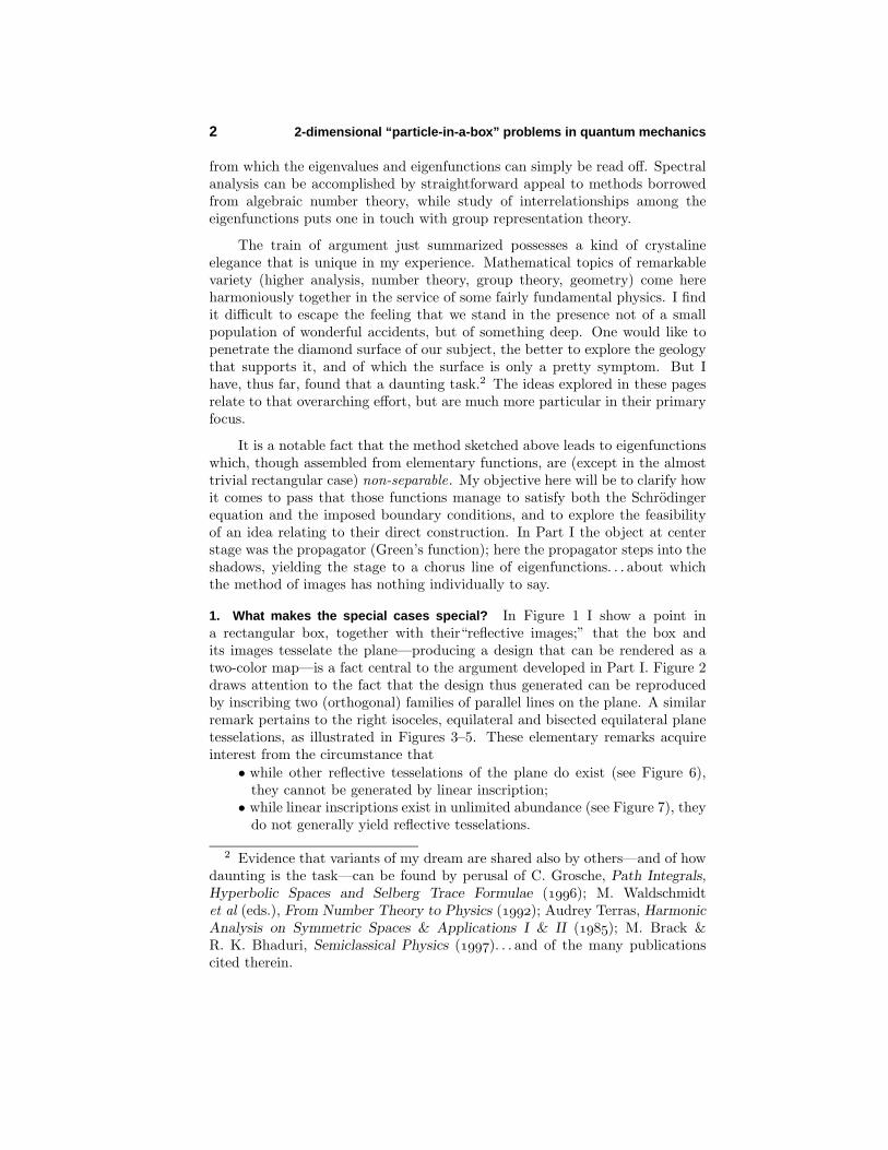
1. What makes the special cases special? In Figure 1 I show a point ina rectangular box, together with their“reflective images;” that the box andits images tesselate the plane—producing a design that can be rendered as atwo-color map—is a fact central to the argument developed in Part I. Figure 2draws attention to the fact that the design thus generated can be reproducedby inscribing two (orthogonal) families of parallel lines on the plane. A similarremark pertains to the right isoceles, equilateral and bisected equilateral planetesselations, as illustrated in Figures 3–5. These elementary remarks acquireinterest from the circumstance that
• while other reflective tesselations of the plane do exist (see Figure 6),they cannot be generated by linear inscription;• while linear inscriptions exist in unlimited abundance (see Figure 7), they
do not generally yield reflective tesselations.
2 Evidence that variants of my dream are shared also by others—and of howdaunting is the task—can be found by perusal of C. Grosche, Path Integrals,Hyperbolic Spaces and Selberg Trace Formulae (); M. Waldschmidtet al (eds.), From Number Theory to Physics (); Audrey Terras, HarmonicAnalysis on Symmetric Spaces & Applications I & II (); M. Brack &R. K. Bhaduri, Semiclassical Physics (). . . and of the many publicationscited therein.

What makes the special cases special? 3
Figure 1: Point in a rectangular box, together with its reflectiveimages. Special importance attached in Part I—but not in thepresent discussion—to the “fundamental unit,” which here has fourelements (outlined), and gives rise translationally to the remainderof the figure.
Figure 2: Reproduction of the preceding figure by superimposedlinear inscripton on the plane.

4 2-dimensional “particle-in-a-box” problems in quantum mechanics
Figure 3: Production of the 45-45-90 tesselation by superpositionof four families of inscribed lines.
Figure 4: Production of the 60-60-60 tesselation by superpositionof three families of inscribed lines.

What makes the special cases special? 5
Figure 5: Production of the 30-60-90 tesselation by superpositionof six families of inscribed lines.
Figure 6: Reflective tesselations that cannot be constructed bysuperposition of families of inscribed lines. Each contains verticesof order three, and therefore cannot be displayed as a two-color map.

6 2-dimensional “particle-in-a-box” problems in quantum mechanics
Figure 7: Ruled tesselations that are not reflective. An analogof the figure on the left can be constructed for any triangle. Therhombus on the right supports also a reflective tesselation (see againthe preceding figure).
The special cases of interest to us are special therefore in (amongst others)this sense: for them—and for them alone—is the reflective tesselation ruled,the ruled tesselation reflective. Reflective tesselation is essential to the methodof images, but ruled tesselation relates most directly to the line of argumentdeveloped below. But the rectangle and its three triangular friends are specialalso in several other respects:
It has been known for a long time3 that “diffraction in the corner of apolygon (exceptionally) does not occur whenever the corner angle is π dividedby an integer.” The following cases
45 + 45 + 90 = 180 : case of the right isoceles triangle60 + 60 + 60 = 180 : case of the equilateral triangle30 + 60 + 90 = 180 : case of the bisected equilateral triangle
90 + 90 + 90 + 90 = 360 : case of the rectangle
therefore exhaust the list of “diffractionless boxes.” The argument here (whichinvolves nothing more sophisticated than direct inspection of the arithmeticpossibilities) is similar to the argument which in led Thomas Wieting toa list of all the (ruled/unruled) reflective tesselations of the plane. Here we seeagain the confluence of physics and geometry which distinguishes the methodof images in all of its manifestations.
3 A. Sommerfeld, Math. Ann. 47, 317 (1896); F. Oberhettinger, J. Res. Natl.Bur. Stand. 61,343 (1958). More immediately germane (because rooted in theFeynman formalism) is R. E. Crandall, “Exact propagator for motion confinedto a sector,” J. Phys. A: Math. Gen. 16, 513 (1983), which provides severaladditional references.

Non-separable eigenfunctions in the equilateral case 7
Our special cases are (though I will not, on the present occasion, attemptto formalize the remark) distinguished from other reflective tesselations also inthe geometrical respect illustrated in Figure 8. This fact brings to mind the
F
F
F
F
F
F FF
FF
F
FF
FF
FF
FF
F
FF
F
FFF
FF
F
FF
FF
F
FFF
FF
F
F
FF
F
FF
F
FF
FFF
F
FF
F
Figure 8: When an equilateral box moves reflectively from onelocation to another its orientation upon arrival is independent ofthe path taken; when it returns to its original location it is returnedalso—in all cases—to its original orientation. Each image of theoriginal box can be assigned therefore an unambiguous “name.” Theother “special boxes” possess also that property, which is basic to thesuccessful application of the method of images. For a demonstrationthat this is a property not shared by (for example) hexagonal boxes,see Figure 8 in Part I.
condition∮
F · dxF · dxF · dx = 0 characteristic of “conservative” forces, and is reminiscentalso of the parallel transport property that serves to characterize the “flatness”of a Riemannian manifold.
2. Non-separable eigenfunctions in the equilateral case. Near the end of §8 inPart I, we obtain eigenfunctions which, relative to the coordinates of Figure 9,can be described
Ψnnn(xxx) ≡√
43·area
{Gnnn(xxx) + iFnnn(xxx)
}where the quantum numbers {n1, n2} range on the interior of the wedge shownin Figure 10, and where the real/imaginary parts of Ψnnn(xxx) can be described4
4 See Part I, pp. 45 & 46.

8 2-dimensional “particle-in-a-box” problems in quantum mechanics
a
h
x
x
Figure 9: Coordinates employed in connection with the equilateralbox problem. The box has
height h = 12
√3a
area = 14
√3a2
Figure 10: The quantum numbers nnn that arise in connection withthe equilateral box problem range (as do those of the closely related30-60-90 box problem) on the interior of the shaded wedge, andalways have the same parity. See Figure 28 in Part I for moredetailed information.
Gnnn(x1, x2) ≡ cos[2n1ξ1] sin[2n2ξ2] + cos[n1(ξ1 + ξ2)] sin[n2(3ξ1 − ξ2)] (1.1)− cos[n1(ξ1 − ξ2)] sin[n2(3ξ1 + ξ2)]
F nnn(x1, x2) ≡ sin[2n1ξ1] sin[2n2ξ2]− sin[n1(ξ1 + ξ2)] sin[n2(3ξ1 − ξ2)] (1.2)+ sin[n1(ξ1 − ξ2)] sin[n2(3ξ1 + ξ2)]
or again (by appeal to some wonderful—if little known—identities)

Non-separable eigenfunctions in the equilateral case 9
G nnn(x1, x2) = cos[2n1ξ1] sin[2n2ξ2] + cos[2−n1+3n22 ξ1] sin[2−n1−n2
2 ξ2] (2.1)
+ cos[2−n1−3n22 ξ1] sin[2+n1−n2
2 ξ2]
F nnn(x1, x2) = sin[2n1ξ1] sin[2n2ξ2] + sin[2−n1+3n22 ξ1] sin[2−n1−n2
2 ξ2] (2.2)
+ sin[2−n1−3n22 ξ1] sin[2+n1−n2
2 ξ2]
where the dimensionless variables ξ1 and ξ2 are defined
ξ1 ≡ π3ax1 and ξ2 ≡ π
3a
√3x2 (3)
The adjustment (1)→ (2) was basic to the progress of the argument developedin Part I, but in the present context it is useful to have both variants at ourdisposal.
How do the functions G nnn(x1, x2) and F nnn(x1, x2) manage to vanish on theboundary of the equilateral box? The box is bounded by (segments of) linesthat can be described
x2 = h : topx2 = +(2h/a)x1 : right sidex2 = −(2h/a)x1 : left side
which in dimensionless variables read
ξ2 = π2
ξ2 = +3ξ1
ξ2 = −3ξ1
(4)
respectively. Working from (2), we have
Gnnn(xxxtop) = cos[2n1ξ1] sin[n2π] + cos[2−n1+3n22 ξ1] sin[−n1−n2
2 π]
+ cos[2−n1−3n22 ξ1] sin[+n1−n2
2 π]= 0 + 0 + 0
F nnn (xxxtop) = sin[2n1ξ1] sin[n2π] + sin[2−n1+3n22 ξ1] sin[−n1−n2
2 π]
+ sin[2−n1−3n22 ξ1] sin[+n1−n2
2 π]= 0 + 0 + 0
because n1 and n2 both even or both odd =⇒ ∓ n1−n22 is (to within a sign) an
integer. Working now from (1), we have
Gnnn(xxxright side) = cos[2n1ξ1] sin[6n2ξ1] + cos[4n1ξ1] sin[n2(3ξ1 − 3ξ1)]− cos[2n1ξ1] sin[n2(3ξ1 + 3ξ1)]
= term + 0− same term = 0
Fnnn(xxxright side) = sin[2n1ξ1] sin[6n2ξ1]− sin[4n1ξ1] sin[n2(3ξ1 − 3ξ1)]− sin[2n1ξ1] sin[n2(3ξ1 + 3ξ1)]
= term + 0− same term = 0
10 2-dimensional “particle-in-a-box” problems in quantum mechanics
Gnnn(xxx left side) and Fnnn(xxx left side) vanish by an identical mechanism. Evidentlythe eigenfunctions vanish “straightforwardly” at the top of the equilateral box,but “by conspiracy” on its sides.
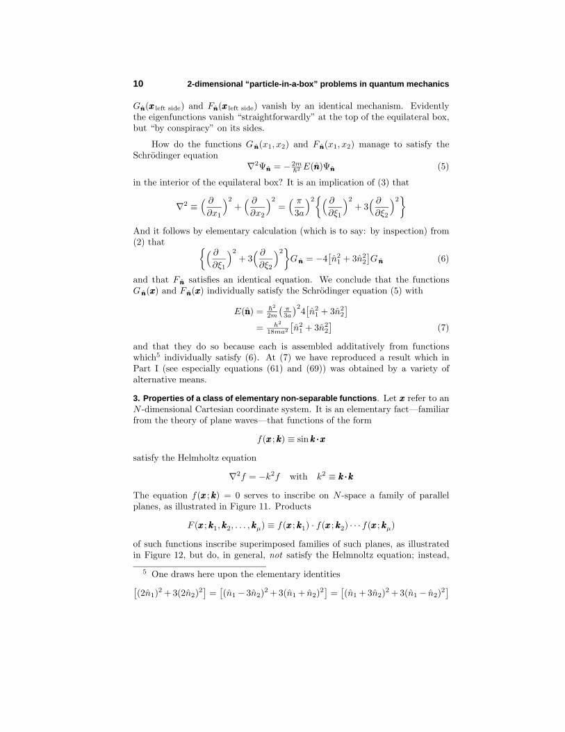
How do the functions G nnn(x1, x2) and F nnn(x1, x2) manage to satisfy theSchrodinger equation
∇2Ψnnn = − 2m�2 E(nnn)Ψnnn (5)
in the interior of the equilateral box? It is an implication of (3) that
∇2 ≡( ∂
∂x1
)2
+( ∂
∂x2
)2
=( π
3a
)2{( ∂
∂ξ1
)2
+ 3( ∂
∂ξ2
)2}
And it follows by elementary calculation (which is to say: by inspection) from(2) that {( ∂
∂ξ1
)2
+ 3( ∂
∂ξ2
)2}
G nnn = −4[n2
1 + 3n22
]G nnn (6)
and that F nnn satisfies an identical equation. We conclude that the functionsG nnn(xxx) and F nnn(xxx) individually satisfy the Schrodinger equation (5) with
E(nnn) = �2
2m
(π3a
)24[n2
1 + 3n22
]= h2
18ma2
[n2
1 + 3n22
](7)
and that they do so because each is assembled additatively from functionswhich5 individually satisfy (6). At (7) we have reproduced a result which inPart I (see especially equations (61) and (69)) was obtained by a variety ofalternative means.
3. Properties of a class of elementary non-separable functions. Let xxx refer to anN -dimensional Cartesian coordinate system. It is an elementary fact—familiarfrom the theory of plane waves—that functions of the form
f(xxx ;kkk) ≡ sink ·xk ·xk ·x
satisfy the Helmholtz equation
∇2f = −k2f with k2 ≡ k ·kk ·kk ·k
The equation f(xxx ;kkk) = 0 serves to inscribe on N -space a family of parallelplanes, as illustrated in Figure 11. Products
F (xxx ;kkk1, kkk2, . . . , kkkµ) ≡ f(xxx ;kkk1) · f(xxx ;kkk2) · · · f(xxx ;kkkµ)
of such functions inscribe superimposed families of such planes, as illustratedin Figure 12, but do, in general, not satisfy the Helmnoltz equation; instead,
5 One draws here upon the elementary identities[(2n1)2 + 3(2n2)2
]=
[(n1− 3n2)2 + 3(n1 + n2)2
]=
[(n1 + 3n2)2 + 3(n1− n2)2
]

Properties of a class of non-separable functions 11
Figure 11: Two-dimensional representation of the null planes off(xxx ;kkk). The planes (lines) are normal to the “wave-vector” kkk andare separated by a distance s = π/k.
Figure 12: Superimposed null lines typical of F (xxx ;kkk1, kkk2, kkk3). Theabsence of periodicity is conspicuous.
12 2-dimensional “particle-in-a-box” problems in quantum mechanics
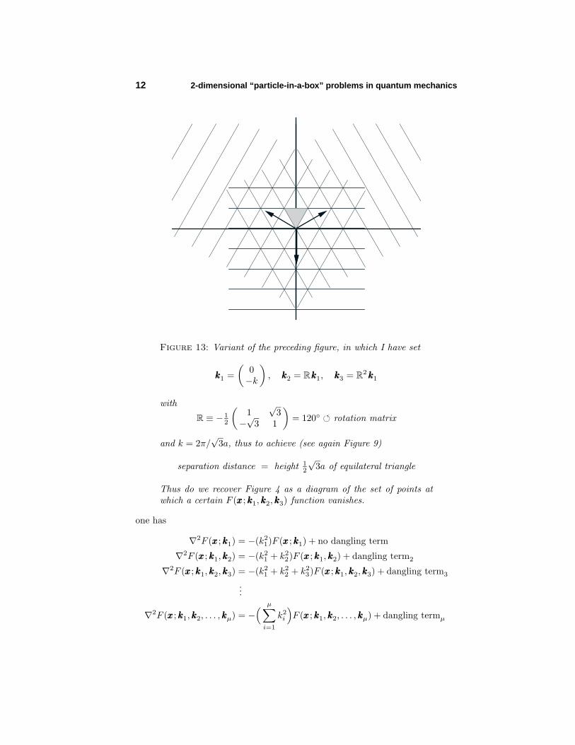
Figure 13: Variant of the preceding figure, in which I have set
kkk1 =(
0−k
), kkk2 = Rkkk1, kkk3 = R
2kkk1
with
R ≡ − 12
(1
√3
−√
3 1
)= 120◦ � rotation matrix
and k = 2π/√
3a, thus to achieve (see again Figure 9)
separation distance = height 12
√3a of equilateral triangle
Thus do we recover Figure 4 as a diagram of the set of points atwhich a certain F (xxx ;kkk1, kkk2, kkk3) function vanishes.
one has
∇2F (xxx ;kkk1) = −(k21)F (xxx ;kkk1) + no dangling term
∇2F (xxx ;kkk1, kkk2) = −(k21 + k2
2)F (xxx ;kkk1, kkk2) + dangling term2
∇2F (xxx ;kkk1, kkk2, kkk3) = −(k21 + k2
2 + k23)F (xxx ;kkk1, kkk2, kkk3) + dangling term3
...
∇2F (xxx ;kkk1, kkk2, . . . , kkkµ) = −( µ∑
i=1
k2i
)F (xxx ;kkk1, kkk2, . . . , kkkµ) + dangling termµ

Properties of a class of non-separable functions 13
wheredangling term2 = 2kkk1·k·k·k2 cos(kkk1·x·x·x) cos(kkk2·x·x·x)dangling term3 = 2kkk1·k·k·k2 cos(kkk1·x·x·x) cos(kkk2·x·x·x) sin(kkk3·x·x·x)
+ 2kkk1·k·k·k3 cos(kkk1·x·x·x) sin(kkk2·x·x·x) cos(kkk3·x·x·x)+ 2kkk2·k·k·k3 sin(kkk1·x·x·x) cos(kkk2·x·x·x) cos(kkk3·x·x·x)
...dangling termµ = etc.
The question now arises: Under what conditions do the “dangling terms”vanish? Clearly
dangling term2 = 0 if kkk1 ⊥ kkk2, which requires N ≥ 2dangling term3 = 0 if kkk1, kkk2 and kkk3 are mutually ⊥ , which requires N ≥ 3
...
These are conditions that come naturally into play when the “particle in a(hyperdimensional) rectangular box” problem is approached by separaton ofvariables. I will not, on this occasion, linger to discuss the evidently moredifficult question “Are the conditions just stated also necessary?”
It is important to notice that for F (xxx ;kkk1, kkk2, kkk3) to be a solution of theHelmholtz equation6 it is not strictly necessary for the associated dangling termactually to vanish; it is sufficient to achieve
dangling term3 ∼ F (xxx ;kkk1, kkk2, kkk3) itself
To illustrate the point, I assign to the wave vectors kkk1, kkk2 and kkk3 the valuesindicated in Figure 13:
kkk1 =(
0−k
), kkk2 = 1
2
(+√
3kk
), kkk2 = 1
2
(−√
3kk
)(8.1)
Thenk21 = k2
2 = k23 = k2 and kkk1· kkk2 = kkk1· kkk3 = kkk2· kkk3 = − 1
2k2 (8.2)
Moreoverkkk1 + kkk2 + kkk3 = 000 (8.3)
which is, by the way, clear from the figure, and consistent with the dot productdata just presented. Drawing upon (8), we have (by some commonplace trickery:introduce a term only to subtract it again)
6 It is, of course, only in the service of expository concreteness that I havehere assigned µ the value 3; the point at issue holds quite generally. But it is,I admit, (and as will soon emerge) a particular instance of the case µ = 3 thatserves primarily to motivate this discussion.

14 2-dimensional “particle-in-a-box” problems in quantum mechanics
dangling term3 =− k2{
cos(kkk1·x·x·x) cos(kkk2·x·x·x) sin(kkk3·x·x·x)
+ cos(kkk1·x·x·x) sin(kkk2·x·x·x) cos(kkk3·x·x·x)+ sin(kkk1·x·x·x) cos(kkk2·x·x·x) cos(kkk3·x·x·x)− sin(kkk1·x·x·x) sin(kkk2·x·x·x) sin(kkk3·x·x·x)
+ sin(kkk1·x·x·x) sin(kkk2·x·x·x) sin(kkk3·x·x·x)}
=− k2{
cos(kkk1·x·x·x) sin([kkk2 + kkk3]·x·x·x)
+ sin(kkk1·x·x·x) cos([kkk2 + kkk3]·x·x·x)
+ sin(kkk1·x·x·x) sin(kkk2·x·x·x) sin(kkk3·x·x·x)}
=− k2{
sin([kkk1 + kkk2 + kkk3]︸ ︷︷ ︸·x·x·x) + sin(kkk1·x·x·x) sin(kkk2·x·x·x) sin(kkk3·x·x·x)︸ ︷︷ ︸ }000 F (xxx ;kkk1, kkk2, kkk3)
Here the dangling term has in fact not vanished, but has returned a weightedreplica of F (xxx ;kkk1, kkk2, kkk3) itself; we conclude that in the equilateral triangularcase (Figure 13)
∇2F (xxx ;kkk1, kkk2, kkk3) = −(3 + 1)k2F (xxx ;kkk1, kkk2, kkk3)
The function F (xxx ;kkk1, kkk2, kkk3) vanishes on the boundary of the trangle, andsatisfies the time-independent Schrodinger equation
− �2
2m∇2F = E · F
withE = �
2
2m4k2 = h2
18ma2 · 12
This is in some respects a curious result. We note, for example, that
12 = 32 + 3 · 12
is associated with the lowest-lying point on the upper edge of the wedge shownin Figure 10, and edge points are excluded according to arguments developedin Part I, where we found the ground state of a particle in an equilateral boxto energy given by
Eground = h2
18ma2 · (52 + 3 · 12)
We acquire, therefore, an obligation to make sense of the result in now in hand.
As a first step in that direction, I observe that
F (xxx ;kkk1, kkk2, kkk3) ≡ sin(kkk1·x·x·x) sin(kkk2·x·x·x) sin(kkk3·x·x·x)
can, with the aid of standard trigonometric identities, be recast
F (xxx ;kkk1, kkk2, kkk3) = 12 sin(kkk1·x·x·x)
{cos([kkk2 − kkk3]·x·x·x)− cos([kkk2 + kkk3]·x·x·x)
}= 1
4
{sin([kkk1 + kkk2 − kkk3]·x·x·x) + sin([kkk1 − kkk2 + kkk3]·x·x·x)
− sin([kkk1 + kkk2 + kkk3]︸ ︷︷ ︸·x·x·x)− sin([kkk1 − kkk2 − kkk3]·x·x·x)}
000 in the equilateral case= − 1
4
{sin(2kkk1·x·x·x) + sin(2kkk2·x·x·x) + sin(2kkk3·x·x·x)
}(9)
Properties of a class of non-separable functions 15
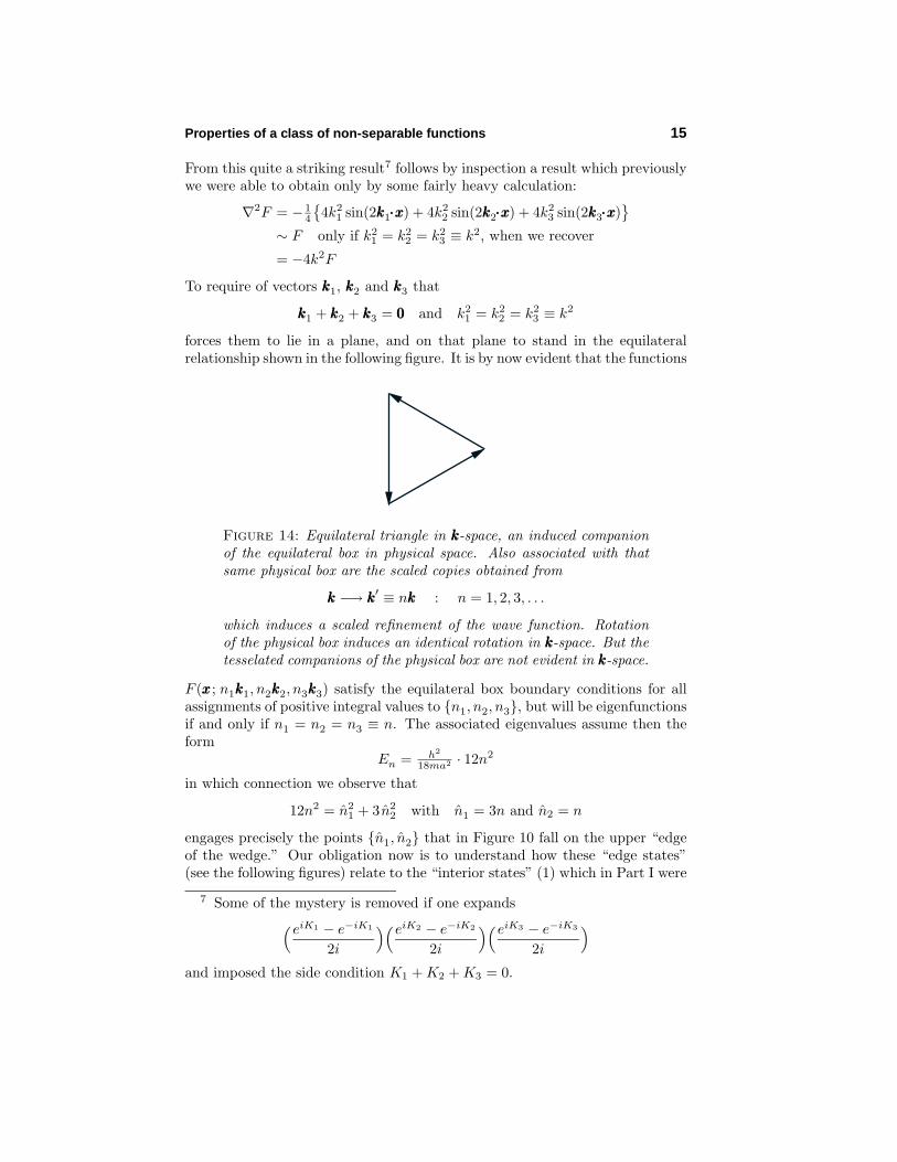
From this quite a striking result7 follows by inspection a result which previouslywe were able to obtain only by some fairly heavy calculation:
∇2F = − 14
{4k2
1 sin(2kkk1·x·x·x) + 4k22 sin(2kkk2·x·x·x) + 4k2
3 sin(2kkk3·x·x·x)}
∼ F only if k21 = k2
2 = k23 ≡ k2, when we recover
= −4k2F
To require of vectors kkk1, kkk2 and kkk3 that
kkk1 + kkk2 + kkk3 = 000 and k21 = k2
2 = k23 ≡ k2
forces them to lie in a plane, and on that plane to stand in the equilateralrelationship shown in the following figure. It is by now evident that the functions
Figure 14: Equilateral triangle in kkk-space, an induced companionof the equilateral box in physical space. Also associated with thatsame physical box are the scaled copies obtained from
kkk −→ kkk′ ≡ nkkk : n = 1, 2, 3, . . .
which induces a scaled refinement of the wave function. Rotationof the physical box induces an identical rotation in kkk-space. But thetesselated companions of the physical box are not evident in kkk-space.
F (xxx ; n1kkk1, n2kkk2, n3kkk3) satisfy the equilateral box boundary conditions for allassignments of positive integral values to {n1, n2, n3}, but will be eigenfunctionsif and only if n1 = n2 = n3 ≡ n. The associated eigenvalues assume then theform
En = h2
18ma2 · 12n2
in which connection we observe that
12n2 = n21 + 3 n2
2 with n1 = 3n and n2 = n
engages precisely the points {n1, n2} that in Figure 10 fall on the upper “edgeof the wedge.” Our obligation now is to understand how these “edge states”(see the following figures) relate to the “interior states” (1) which in Part I were
7 Some of the mystery is removed if one expands(eiK1 − e−iK1
2i
)(eiK2 − e−iK2
2i
)(eiK3 − e−iK3
2i
)and imposed the side condition K1 + K2 + K3 = 0.
16 2-dimensional “particle-in-a-box” problems in quantum mechanics
-1 -0.5 0 0.5 1-1
-0.5
0
0.5
1
-1 -0.5 0 0.5 1-1
-0.5
0
0.5
1
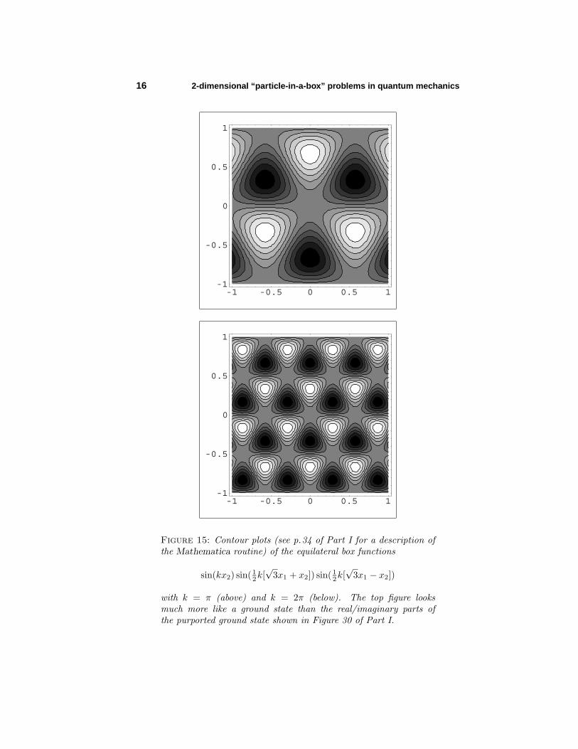
Figure 15: Contour plots (see p.34 of Part I for a description ofthe Mathematica routine) of the equilateral box functions
sin(kx2) sin( 12k[√
3x1 + x2]) sin(12k[√
3x1 − x2])
with k = π (above) and k = 2π (below). The top figure looksmuch more like a ground state than the real/imaginary parts ofthe purported ground state shown in Figure 30 of Part I.

Properties of a class of non-separable functions 17
-1 -0.5 0 0.5 1-1
-0.5
0
0.5
1
-1 -0.5 0 0.5 1-1
-0.5
0
0.5
1
Figure 16: Nodal curves (lines) of the equilateral box states shownin the preceding figure. The figures are self-similar in the sensediscussed on p.83 of Part I, and display the design anticipatedalready in Figures 4 & 13.
were obtained by the method of images. To facilitate discussion of that topic,we observe that introduction of (8.1) into (9) gives
F = 14
{sin(2kx2) + sin(k[
√3x1 − x2])− sin(k[
√3x1 + x2])
}which in the dimensionless ξ-variables introduced at (3) becomes

18 2-dimensional “particle-in-a-box” problems in quantum mechanics
F = 14
{sin(2k 3a
π√
3ξ2) + sin(k[
√3 3a
π ξ1 − 3aπ√
3ξ2])− sin(k[
√3 3a
π ξ1 + 3aπ√
3ξ2])
}Finally (see again the captions to Figures 14 & 13) we make the replacements
k −→ nk −→ n 2π√3a
and are led to the functions
Hn(x1, x2) ≡ sin[2n(2ξ2)] + sin[2n(3ξ1 − ξ2)]− sin[2n(3ξ1 + ξ2)]= sin[4nξ2]− 2 cos[6nξ1] · sin[2nξ2]
}(10)
4. Relationship to eigenfunctions obtained by method of images. Looking backagain to (1) it becomes immediately evident that we have only to set
nnn =(
02n
)
to obtainGnnn(x1, x2) = Hn(x1, x2)F nnn(x1, x2) = 0
But in §8 of Part I we were at pains to establish that the “axial” lattice point(02n
)and the “upper edge of the wedge” point
(3nn
)are equivalent in the duplex
Figure 17: The axial point(
02n
)is equivalent to the “wedge-edge”
point(
3nn
), and is the “seed” from which sprout a population of
associated points(
3nn+2k
). For finer details, see Figure 27 in Part I
and associated text.
Relationship to eigenfunctions obtained by method of images 19
sense that the eigenvalues
E(nnn) = h2
18ma2 [ n21 + 3 n2
2 ]↓= h2
18ma2 12n2 when nnn =(
02n
)are invariant under
(02n
)−→
(3nn
), and so also (to within an overall sign) are
the associated eigenfunctions8
G nnn(x1, x2) = cos[2n1ξ1] sin[2n2ξ2] + cos[2−n1+3n22 ξ1] sin[2−n1−n2
2 ξ2]
+ cos[2−n1−3n22 ξ1] sin[2+n1−n2
2 ξ2]↓= Hn(x1, x2) when nnn =
(02n
)To summarize: drawing motivation from the observation that reflective
tesselations of the plane yield to analysis by the method of images if andonly if they are at the same time ruled tesselations (and vice versa: ruledtesselations are tractable if and only if they are reflective), we looked in §3 tosome elementary functions whose zeros rule the plane, and were led at lengthto a population Hn(x1, x2) of equilateral box eigenfunctions which are noneother than the G nnn(x1, x2) associated with lattice points nnn that are positionedon the upper edge of the wedge. The argument did serve to expose a majorerror in Part I, which stands therefore in need of revision,9 but was found tosuffer from its own intrinsic limitations: it provides no direct insight into theorthonormality properties of the Hn(x1, x2) functions, and it fails to accountfor the eigenfunctions identified by lattice points interior to the wedge. Itis clear that the functions G nnn(x1, x2) and F nnn(x1, x2), since known on othergrounds to be (when nnn lies interior to the wedge) linearly independent of thefunctions Hn(x1, x2), cannot be developed as linear combinations of the latter.Nor can they contain Hn(x1, x2) functions as factors—else they would exhibitequilaterally arranged patterns of nodal lines, which manifestly they do not do.
I turn now to discussion of a train of thought that first occurred to me whileconstructing figures10 in quite another connection, but which has a acquired newinterest as a possible means of escape from the limitations just ennumerated.
8 I quote here from (2). Similarly invariant—in the trivial sense 0 = 0—arethe companion eigenfunctions F nnn(x1, x2).
9 It follows by inspection from (1) that G nnn(x1, x2) and F nnn(x1, x2) bothvanish when nnn lies on the lower edge of the wedge (n2 = 0), and that F nnn(x1, x2)vanishes also on the upper edge (equivalent to n1 = 0), but I was in errorwhen (on p. 51 of Part I) I claimed that G nnn(x1, x2) vanishes on the upperedge; it manifestly does not. I was, for this reason, wrong when (on thatsame page) I asserted that every equilateral box eigenvalue “is, in the absenceof accidental degeneracy, doubly degenerate; ” wrong when, in Figure 30, Iclaimed to providing representions the equilateral ground state(s); wrong so faras concerns some of the spectral density details presented in §9.
10 See especially Figure 48 in Part I.

20 2-dimensional “particle-in-a-box” problems in quantum mechanics
5. Method of sections. Let our mass point m be constrained now to movefreely within the rectangular 3-dimensional box shown in the following figure.Holding xxx-variables in reserve, we write yyy to describe points in the 3-space
Figure 18: Generic rectangular box, of volume b1b2b3, withinwhich a mass point m moves freely. It is by refinement of thiselementary construction that we are led to the systems to which the“method of sections” pertains. We will have interest mainly in thecubic case b1 = b2 = b3 ≡ b.
within which the box resides. Looking to the elementary time-independentquantum mechanics of such a system, one is led—whether one proceeds byseparation of variables, by the method of images, or (perhaps most efficiently)by the methods developed in §3—to eigenfunctions of the form
Ψ(yyy) ∼ sin(n1πb1
y1) sin(n2πb2
y2) sin(n3πb3
y3)↓= sin(n1
πb y1) sin(n2
πb y2) sin(n3
πb y3) in the cubic case (11)
The associated eigenvalues are given by
E(nnn) =h2
8mb2[n2
1 + n22 + n2
3]
Such product functions serve to partition yyy -space into stacked rectangles, whichin the cases of immediate interest become stacked cubes (see Figure 19).
Method of sections 21
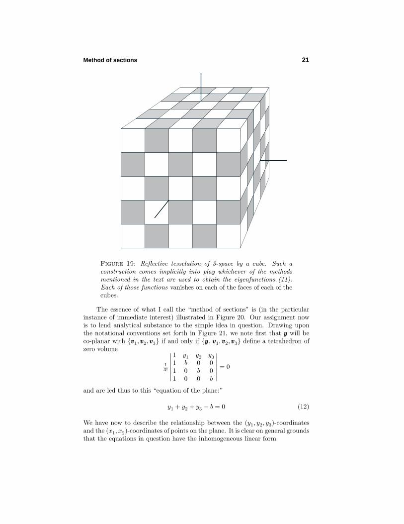
Figure 19: Reflective tesselation of 3-space by a cube. Such aconstruction comes implicitly into play whichever of the methodsmentioned in the text are used to obtain the eigenfunctions (11).Each of those functions vanishes on each of the faces of each of thecubes.
The essence of what I call the “method of sections” is (in the particularinstance of immediate interest) illustrated in Figure 20. Our assignment nowis to lend analytical substance to the simple idea in question. Drawing uponthe notational conventions set forth in Figure 21, we note first that yyy will beco-planar with {vvv1, vvv2, vvv3} if and only if {yyy , vvv1, vvv2, vvv3} define a tetrahedron ofzero volume
13!
∣∣∣∣∣∣∣1 y1 y2 y3
1 b 0 01 0 b 01 0 0 b
∣∣∣∣∣∣∣ = 0
and are led thus to this “equation of the plane:”
y1 + y2 + y3 − b = 0 (12)
We have now to describe the relationship between the (y1, y2, y3)-coordinatesand the (x1, x2)-coordinates of points on the plane. It is clear on general groundsthat the equations in question have the inhomogeneous linear form

22 2-dimensional “particle-in-a-box” problems in quantum mechanics
Figure 20: The equilaterally tesselated plane (below) has beenobtained by “sanding off the corner” of (i.e., as a plane section of)the cubically tesselated 3-space shown above (see also Figure 19).The figure exposes the central idea of what I call the “method ofsections.”

Method of sections 23
y
x
y
y
x
p
Figure 21: Notations used in discussion of the method of sections,as it relates to the equilateral box problem. The cube has sides oflength b and vertices at the points
000
,
b
00
,
0
b0
,
0
0b
︸ ︷︷ ︸,
0
bb
,
b
0b
,
b
b0
and
b
bb
vertices {vvv1, vvv2, vvv3} of the
The plane is perpendicular to the semi-diagonal vector
ppp ≡ 12
b
bb
The triangle has sides of length a =√
2b. The xxx-coordinate system(inscribed on the plane, oriented as shown, with origin at vvv1) standsto the triangle in a relation imitative of Figure 9.

24 2-dimensional “particle-in-a-box” problems in quantum mechanics
y1 = A11x1 + A12x2 + B1
y2 = A21x1 + A22x2 + B2
y3 = A31x1 + A32x2 + B3
of which, however, we need consider only two, since the third will follow from(12); we look to the last two, since y2 and y3 stand in a symmetrical relationship(and y1 in an eccentric relationship) to the x-coordinate system. Lookingspecifically to the vertices of the triangle, it becomes clear that the coefficients{A21, A22, A31, A32, B2, B3} must satisfy
0 = A210 + A220 + B2
0 = A310 + A320 + B3
}at vvv1
b = +A21a2 + A22h + B2
0 = +A31a2 + A32h + B3
}at vvv2
0 = −A21a2 + A22h + B2
b = −A31a2 + A32h + B3
}at vvv3
where (see again the captions to Figures 9 & 21) a2 = 1√
2b and h = 1
2
√6b.
It follows from the top pair of equations that B2 = B3 = 0. The remainingequations can therefore be written
+ 1
2a h 0 00 0 + 1
2a h− 1
2a h 0 00 0 − 1
2a h
A21
A22
A31
A32
=
b00b
which by marix inversion give
A21 = + ba = + 1√
2
A22 = b2h = 1√
6
A31 = − ba = − 1√
2
A32 = b2h = 1√
6
Thus do we obtainy1 = − 2√
6x2 + b
y2 = + 1√2x1 + 1√
6x2
y3 = − 1√2x1 + 1√
6x2
(13)
where the top equation was obtained from the latter pair by appeal to (12).Drawing upon this result, we learn that the functions
Znnn(y1, y2, y3) ≡ sin(n1πb y1) sin(n2
πb y2) sin(n3
πb y3) (14)

Method of sections 25
assume values on the plane which can, in x-coordinates, be described
Znnn(x1, x2) ≡ sin[n1
πb
(− 2√
6x2 + b
)]· sin
[n2
πb
(+ 1√
2x1 + 1√
6x2
)](15)
· sin[n3
πb
(− 1√
2x1 + 1√
6x2
)]where {n1, n2, n3} range independently/unrestrictedly on the positive integers.It becomes appropriate at this point to replace the cube scale parameter b withthe triangle scale parameter a =
√2b; we obtain
Znnn(x1, x2) ≡ sin[n1
πa
2√3x2 − n1π
]· sin
[n2
πa
(x1 + 1√
3x2
)]· sin
[n3
πa
(x1 − 1√
3x2
)]in which connection we notice that the leading factor
sin[n1
πa
2√3x2 − n1π
]= (−)n1 sin
[n1
πa
2√3x2
]In terms of the dimensionless ξ-variables introduced at (3) we have
Znnn(x1, x2) = (−)n1Wnnn(x1, x2)
where
Wnnn(x1, x2) ≡ sin[2n1ξ2
]· sin
[n2
(3ξ1 + ξ2
)]· sin
[n3
(3ξ1 − ξ2
)](16.1)
can, in the notation of §3, be written
= sin(kkk1·x·x·x) · sin(kkk2·x·x·x) · sin(kkk3·x·x·x) (16.2)
where
kkk1 = n1k
(0−2
), kkk2 = n2k
(+√
31
)and kkk3 = n3k
(−√
31
)
stand (or at least they do when n1 = n2 = n3 = n )in the relationship familiarfrom Figure 14; here as before, k ≡ π√
3a.
It is by now abundantly clear that the “method of sections,” as thus fardeveloped, has led us back again to precisely the population of functions, andto the set of ideas, familiar from §3. Back again, but no farther. Both linesof argument supply infinite populations of functions each of which satisfies theequilateral box boundary conditions and some of which (the functions Hn(x1, x2)discussed in §4) are in fact eigenfunctions as they stand. The question still open:Is it possible, with the material thus provided, to assemble the remainder ofthe “interior” eigenfunctions (1)?

26 2-dimensional “particle-in-a-box” problems in quantum mechanics
6. Assembly of eigenfunctions in the equilateral case. We undertake now toexplore the possibility of representing functions of type (1)—eigenfunctions ofthe equilateral box problem—as linear combinations of functions to type (16.1).To simplify the discussion, I will for the moment restrict my remarks to eigen-functions of “type G,” as defined at (1.1); eigenfunctions of “type F ” will bediscussed separately. As a preparatory step, intended to facilitate comparisons,we render the functions of interest to us into a common (which is to say, ashared) language. Drawing upon Mathematica’s TrigReduce[expr] resource,we obtain
Gnnn(x1, x2) ≡ cos[2n1ξ1] sin[2n2ξ2] + cos[n1(ξ1 + ξ2)] sin[n2(3ξ1 − ξ2)]− cos[n1(ξ1 − ξ2)] sin[n2(3ξ1 + ξ2)]
= 12
{− sin [2 n1ξ1 − 2 n2ξ2] + sin [2 n1ξ1 + 2 n2ξ2] (19.1)− sin [n1(ξ1 + ξ2) − n2(3ξ1 − ξ2)] + sin [n1(ξ1 + ξ2) + n2(3ξ1 − ξ2)]+ sin [n1(ξ1 − ξ2) − n2(3ξ1 + ξ2)] − sin [n1(ξ1 − ξ2) + n2(3ξ1 + ξ2)]
}= 1
2
{− sin [2 n1ξ1 − 2 n2ξ2] + sin [2 n1ξ1 + 2 n2ξ2] (19.2)
− sin [(n1 − 3n2)ξ1 + (n1 + n2)ξ2]+ sin [(n1 + 3n2)ξ1 + (n1 − n2)ξ2]+ sin [(n1 − 3n2)ξ1 − (n1 + n2)ξ2]− sin [(n1 + 3n2)ξ1 − (n1 − n2)ξ2]
}and
Wnnn(x1, x2) ≡ sin[− 2n1ξ2
]· sin
[n2
(+ 3ξ1 + ξ2
)]· sin
[n3
(− 3ξ1 + ξ2
)]= 1
4
{W1 + W2 + W3 + W4
}(20.1)
where
W1 ≡ − sin[2n1ξ2 + n2(3ξ1 + ξ2) + n3(3ξ1 − ξ2)]= − sin[(3n2 + 3n3)ξ1 + (2n1 + n2 − n3)ξ2]
W2 ≡ − sin[2n1ξ2 − n2(3ξ1 + ξ2) − n3(3ξ1 − ξ2)]= + sin[(3n2 + 3n3)ξ1 − (2n1 − n2 + n3)ξ2]
(20.2)W3 ≡ + sin[2n1ξ2 + n2(3ξ1 + ξ2) − n3(3ξ1 − ξ2)]
= + sin[(3n2 − 3n3)ξ1 + (2n1 + n2 + n3)ξ2]
W4 ≡ + sin[2n1ξ2 − n2(3ξ1 + ξ2) + n3(3ξ1 − ξ2)]= − sin[(3n2 − 3n3)ξ1 − (2n1 − n2 − n3)ξ2]
When editing and transcribing results reported by Mathematica it is easy tomake typographic errors; evidence that my work has been accurate is, however,supplied by the following observations:

Assembly of eigenfunctions in the equilateral case 27
Whether one proceeds from (19.1) or from (19.2), one obtains easily thefamiliar “bottom of the wedge” statement G(2n, 0) = 0,11 which is comforting,but too simple to be very informative. Similarly direct are the statements
G(0, 2n) = sin[4nξ2] + sin[6nξ1 − 2nξ2] − sin[6nξ1 + 2nξ2]= 4W (n, n, n)
which are familiar from the discussion that culminated in (10). Recalling
∇2 ≡( ∂
∂x1
)2
+( ∂
∂x2
)2
=( π
3a
)2{( ∂
∂ξ1
)2
+ 3( ∂
∂ξ2
)2}
from near the end of §2, we find it to be—for the interesting reason that
(2n1)2 + 3(2n2)
2 = (n1 − 3n2)2 + 3(n1 + n2) = (n1 + 3n2)
2 + 3(n1 − n2)
—an almost immediate implication of (19.2) that{( ∂
∂ξ1
)2
+ 3( ∂
∂ξ2
)2}
G = −4[n2
1 + 3n22
]G (21)
which reproduces (6). Proceeding similarly from (20) we obtain{( ∂
∂ξ1
)2
+ 3( ∂
∂ξ2
)2}
W = − 12[n21 + n2
2 + n23 + (+n1n2 + n2n3 − n3n1)]
14W1
− 12[n21 + n2
2 + n23 + (−n1n2 + n2n3 + n3n1)]
14W2
− 12[n21 + n2
2 + n23 + (+n1n2 − n2n3 + n3n1)]
14W3
− 12[n21 + n2
2 + n23 + (−n1n2 − n2n3 − n3n1)]
14W4
= −12[n21 + n2
2 + n23]W − 3(+n1n2 + n2n3 − n3n1)W1 (22)
− 3(−n1n2 + n2n3 + n3n1)W2
− 3(+n1n2 − n2n3 + n3n1)W3
− 3(−n1n2 − n2n3 − n3n1)W4
The expression on the right is so intricate and—on its face—strange lookingthat we can expect only with unaccustomed effort to establish its equivalenceto results already in hand. We begin by observing that on the upper edge ofthe wedge (21) reads{( ∂
∂ξ1
)2
+ 3( ∂
∂ξ2
)2}
G(0, 2n) = −48n2G(0, 2n)
11 I will write G(n1, n2) when I want to emphasize the nnn-dependence ofGnnn(x1, x2), and G(ξ1, ξ2) to indicate that I am looking to the xxx-dependencebut have switched to ξξξ variables. The notations W (n1, n2, n3) and W (ξ1, ξ2)will be used with similar intent.

28 2-dimensional “particle-in-a-box” problems in quantum mechanics
while from (22) we obtain{( ∂
∂ξ1
)2
+ 3( ∂
∂ξ2
)2}
W (n, n, n) = − 12[3 + 1]n2 14W1(n, n, n)
− 12[3 + 1]n2 14W2(n, n, n)
− 12[3 + 1]n2 14W3(n, n, n)
− 12[3 − 3]n2 14W4(n, n, n)
W4 is killed on the right, but it is an implication of (20.2) that W4(n, n, n) = 0,so W4 is in fact absent also on the left; we have{( ∂
∂ξ1
)2
+ 3( ∂
∂ξ2
)2}
W (n, n, n) = −48n2W (n, n, n)
as anticipated. The relevant general “result already in hand” was developed in§3, and reads
∇2 sin(kkk1·x·x·x) · sin(kkk2·x·x·x) · sin(kkk3·x·x·x)
= −[k21 + k2
2 + k23] sin(kkk1·x·x·x) · sin(kkk2·x·x·x) · sin(kkk3·x·x·x) + dangling term
wheredangling term = 2kkk1·k·k·k2 cos(kkk1·x·x·x) cos(kkk2·x·x·x) sin(kkk3·x·x·x)
+ 2kkk1·k·k·k3 cos(kkk1·x·x·x) sin(kkk2·x·x·x) cos(kkk3·x·x·x)+ 2kkk2·k·k·k3 sin(kkk1·x·x·x) cos(kkk2·x·x·x) cos(kkk3·x·x·x)
Taking our kkk-vectors from p. 25, we have
[k21 + k2
2 + k23] = 4k2[n2
1 + n22 + n2
3]
2kkk1·k·k·k2 = −4k2n1n2
2kkk1·k·k·k3 = −4k2n1n3
2kkk2·k·k·k3 = −4k2n2n3
where again k ≡ π√3a
. Changing variables xxx −→ ξξξ, we on the basis of theseremarks have
13
{( ∂
∂ξ1
)2
+ 3( ∂
∂ξ2
)2}
sin[− 2n1ξ2
]· sin
[n2
(3ξ1 + ξ2
)]· sin
[n3
(− 3ξ1 + ξ2
)]= −4[n2
1 + n22 + n2
3] sin[− 2n1ξ2
]· sin
[n2
(3ξ1 + ξ2
)]· sin
[n3
(− 3ξ1 + ξ2
)]− 4
{n1n2P3 + n1n3P2 + n2n3P1
}where the 1
3 arose from ( π3a )2 = 1
3k2 (the k2 was then abandoned both left andright) and where the product functions
P3 ≡ cos[− 2n1ξ2
]· cos
[n2
(+ 3ξ1 + ξ2
)]· sin
[n3
(− 3ξ1 + ξ2
)]P2 ≡ cos
[− 2n1ξ2
]· sin
[n2
(+ 3ξ1 + ξ2
)]· cos
[n3
(− 3ξ1 + ξ2
)]P1 ≡ sin
[− 2n1ξ2
]· cos
[n2
(+ 3ξ1 + ξ2
)]· cos
[n3
(− 3ξ1 + ξ2
)]

Assembly of eigenfunctions in the equilateral case 29
Drawing again upon Mathematica’s TrigReduce[expr] resource, we find
P3 = 14
{+ W1 − W2 + W3 − W4
}P2 = 1
4
{− W1 + W2 + W3 − W4
}P1 = 1
4
{+ W1 + W2 − W3 − W4
}Returning with this information to the equation in which P1, P2 and P3 madetheir first appearance, we obtain{( ∂
∂ξ1
)2
+ 3( ∂
∂ξ2
)2}
W = −12[n21 + n2
2 + n23]W
− 3n1n2
{+ W1 − W2 + W3 − W4
}− 3n1n3
{− W1 + W2 + W3 − W4
}− 3n2n3
{+ W1 + W2 − W3 − W4
}= −12[n2
1 + n22 + n2
3]W− 3(+n1n2 + n2n3 − n3n1)W1
− 3(−n1n2 + n2n3 + n3n1)W2
− 3(+n1n2 − n2n3 + n3n1)W3
− 3(−n1n2 − n2n3 − n3n1)W4
which does in fact precisely reproduce (22). I proceed in confidence thatequations (19) and (20) are indeed correct; though they were obtained by whatMathematica calls “trigonometric reduction,” they provide what are in factsimply Fourier sine expansions of the functions G and W .
My objective is to construct a formula of the type
G(n1, n2) =∑
n1n2n3
weighted W -functions (23)
but I lack any straightforwardly computional means for getting from here tothere; I have seemingly no option but to proceed by “incremental insight,” andit is in that spirit that I assemble the following miscellaneous remarks.
It was established in §8 of Part I that—independently of any assumptionthat n1 and n2 be integers—the function
N(n1, n2) ≡ n21 + 3n2
2
is invariant under the linear transformations nnn → Annn → A2nnn where
A ≡ 12
(−1 +3−1 −1
)has the properties
A3 = I and A
TGA = G with G ≡
(1 00 3
)

30 2-dimensional “particle-in-a-box” problems in quantum mechanics
Specifically (n1
n2
)−→
(12 [−n1 + 3n2]12 [−n1 − n2]
)−→
(12 [−n1 − 3n2]12 [+n1 − n2]
)(24.1)
N(n1, n2) is invariant also under the reflective transformations(n1
n2
)−→
(−n1
+n2
)else
(+n1
−n2
)else
(−n1
−n2
)(24.2)
The properties that attach to N(n1, n2) attach also to the functions G(n1, n2)(which were, after all, generated by a process that involved “summing overspectral symmetries”—summing, that is to say, over the symetries of N(n1, n2));Mathematica, working from (19.2), readily confirms that
G(n1, n2) = G( 12 [−n1 + 3n2],
12 [−n1 − n2]) = G( 1
2 [−n1 − 3n2],12 [+n1 − n2])
= +G(−n1,+n2) = −G(+n1,−n2) = −G(−n1,−n2)
and—remarkably—does so independently of any assumption that n1 and n2 beintegers. So far as concerns the ξξξ-dependence of G, Mathematica confirms that
G(ξ1, ξ2) = G(−ξ1, ξ2)
The G-properties assembled above do not (or at least do not in their totality)attach to the functions W , but must perforce attach to the anticipated linearcombinations of W -functions; I propose to use that fact as a design principle.
Passing over now from the G to the W side of the street, we encounter thecircumstance that {n1, n2, n3} are too numerous. Tinkering (inspired partly bythe symmetry evident in (8.3)) leads me tentatively to require
n1 + n2 + n3 = 0 (25)
and to automate that condition by writing
n1 = n1(n1, n2) ≡ 2n2
n2 = n2(n1, n2) ≡ +n1 − n2
n3 = n3(n1, n2) ≡ −n1 − n2
(26)
Thenn2
1 + n22 + n2
3 = 2[n21 + 3n2
2]
The transformations described at the top of the page induce n1
n2
n3
−→
n3
n1
n2
−→
n2
n3
n1
: cyclic (27.1)
−→
+n1
+n3
+n2
else
−n1
−n3
−n2
else
−n1
−n2
−n3
(27.2)

Assembly of eigenfunctions in the equilateral case 31
Looking to the structure of (22) we are motivated to define
w1(n1, n2, n3) ≡ +n1n2 + n2n3 − n3n1
w2(n1, n2, n3) ≡ −n1n2 + n2n3 + n3n1
w3(n1, n2, n3) ≡ +n1n2 − n2n3 + n3n1
w4(n1, n2, n3) ≡ −n1n2 − n2n3 − n3n1
(28)
in which notation (22) reads{( ∂
∂ξ1
)2
+ 3( ∂
∂ξ2
)2}
W = −12[n21 + n2
2 + n23]W
− 3{w1W1 + w2W2 + w3W3 + w4W4
}We observe in this connection that nnn → Annn → A
2nnn induces
w1
w2
w3
w4
−→
w3
w1
w2
w4
−→
w2
w3
w1
w4
(29)
which is again cyclic except in this detail:
w4 = n21 + 3n2
2 transforms by invariance
Nor is this last equation a surprise; it follows from
(n1 + n2 + n3)2 = 02
= (n21 + n2
2 + n23)︸ ︷︷ ︸ +2 (n1n2 + n2n3 + n3n1)︸ ︷︷ ︸
2[n21 + 3n2
2] − w4
At (19) we encounter the display
G ={
sum of eigenfunctions, each with the same eigenvalue,which collectively satisfy the imposed boundary conditions
while at (20) we have
W ={
sum of eigenfunctions with distinct eigenvalues,which collectively satisfy the imposed boundary conditions
In exploratory work (not reported here) I have been tripping over implicationsof the latter fact, and am led to look now therefore to properties of W4, whichis, as we have several times had occasion to notice, a “distinguished member”of the population {W1, W2, W3, W4}. We have{( ∂
∂ξ1
)2
+ 3( ∂
∂ξ2
)2}
W4 = −12[n21 + n2
2 + n23 − n1n2 − n2n3 − n3 − n1]W4
= −12[ 32 (n21 + n2
2 + n23)]W4 when n1 + n2 + n3 = 0
32 2-dimensional “particle-in-a-box” problems in quantum mechanics
Let us, in structural imitation of (26), write
n1 = 2m2
n2 = +m1 − m2
n3 = −m1 − m2
We then have
{( ∂
∂ξ1
)2
+ 3( ∂
∂ξ2
)2}
W4 = −36[m21 + 3m2
2]W4
= −4[n21 + 3n2
2]W4 if m1 ≡ 13 n1 and m2 ≡ 1
3 n2
withW4 = W4
( 2n23 , +n1−n2
3 , −n1−n23
)= − sin[2n1ξ1 − 2n2ξ2]
and are led by this result—taken in conjunction with (27)—to the observationthat12
W4
( 2n23 , +n1−n2
3 , −n1−n23
)= − sin[2n1ξ1 − 2n2ξ2]
W4
(−n1−n23 , 2n2
3 , +n1−n23
)= + sin[(n1 − 3n2)ξ1 − (n1 + n2)ξ2]
W4
(+n1−n23 , −n1−n2
3 , 2n23
)= + sin[(n1 + 3n2)ξ1 + (n1 − n2)ξ2]
W4
( 2n23 , −n1−n2
3 , +n1−n23
)= + sin[2n1ξ1 + 2n2ξ2]
W4
(−n1−n23 , +n1−n2
3 , 2n23
)= − sin[(n1 − 3n2)ξ1 + (n1 + n2)ξ2]
W4
(+n1−n23 , 2n2
3 , −n1−n23
)= − sin[(n1 + 3n2)ξ1 − (n1 − n2)ξ2]
The functions on the right are precisely the six functions which (see again (19.2))when added together give G(n1, n2).
What, in the same vein, can one say of the functions W1, W2 and W3 thatcollaborate with W4 in the assembly of W? Looking to the definitions (28) and
12 Here I omit six equations on these grounds made evident by (20.2):
Wi(−n1,−n2,−n3) = −Wi(n1, n2, n3) : i = 1, 2, 3, 4
This “reflection principle”—elementary though it is—will soon acquire someimportance.

Assembly of eigenfunctions in the equilateral case 33
(20.2) of the functions wi(n1, n2, n3) and Wi(n1, n2, n3), we notice that n1
n2
n3
→
−n1
+n2
+n3
induces
w1
w2
w3
w4
→
w2
w1
w4
w3
&
W1
W2
W3
W4
→
−W2
−W1
−W4
−W3
n1
n2
n3
→
+n1
−n2
+n3
induces
w1
w2
w3
w4
→
w4
w3
w2
w1
&
W1
W2
W3
W4
→
−W4
−W3
−W2
−W1
n1
n2
n3
→
+n1
+n2
−n3
induces
w1
w2
w3
w4
→
w3
w4
w1
w2
&
W1
W2
W3
W4
→
−W3
−W4
−W1
−W2
The preceding equations describe consequences of what are in effect improperrotations in 3-dimensional nnn-space. A clearer sense of what is going on can beobtained if (by compounding the preceding transformations) one looks to theassociated proper rotations; the induced transformations are then permutational(no intrusive signs):
n1
n2
n3
→
+n1
−n2
−n3
induces
w1
w2
w3
w4
→
w2
w1
w4
w3
&
W1
W2
W3
W4
→
W2
W1
W4
W3
n1
n2
n3
→
−n1
+n2
−n3
induces
w1
w2
w3
w4
→
w4
w3
w2
w1
&
W1
W2
W3
W4
→
W4
W3
W2
W1
n1
n2
n3
→
−n1
−n2
+n3
induces
w1
w2
w3
w4
→
w3
w4
w1
w2
&
W1
W2
W3
W4
→
W3
W4
W1
W2
That these induced transformation can be interpreted as having to do with asubgroup of the tetrahedral group is demonstrated in Figure 22.13 The figureserves at the same time to cast new light on other matters as well; it becomesnatural, for example, to interpret (29) as having to do with certain otherrotations in nnn-space—a different subgroup of the tetrahedral group. It is tolend substance to that remark that I now digress:
To describe (relative to a right-handed frame in 3-space) a rotation throughangle ϕ (in the right-handed sense) about the unit vector λλλ one writes
xxx → xxx ′ = R(λλλ, ϕ)xxx
13 The idea embodied in the figure, we note in passing, springs quite naturallyfrom the “method of sections,” but might have escaped our notice had we hadat our disposal only the methods of §3.

34 2-dimensional “particle-in-a-box” problems in quantum mechanics
W
W
W
W
Figure 22: The functions W1, W2, W3 and W4 have been associatedwith the vertices of a tetrahedron inscribed within the cube familiarfrom Figure 21 (except that the present figure lives not in xxx-spacebut in nnn-space). The boldface coordinate system has its origin atthe shared center of the cube and tetrahedron (“center of mass” ofthe construction). 180◦ rotations about the ©1 , ©2 and ©3 axes giverise to the transformations described at the bottom of the precedingpage.
with14
R(λλλ, ϕ) = eϕA = P + (cos ϕ · I + sinϕ · A)(I − P)
where the antisymmetric matrix A inherits its structure from λλλ
A ≡
0 −λ3 λ2
λ3 0 −λ1
−λ2 λ1 0
where
P ≡ A2 + I =
λ1λ1 λ1λ2 λ1λ3
λ2λ1 λ2λ2 λ2λ3
λ3λ1 λ3λ2 λ3λ3
14 See, for example, classical dynamics (-), Chapter I, p. 84.
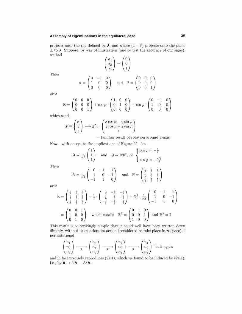
Assembly of eigenfunctions in the equilateral case 35
projects onto the ray defined by λλλ, and where (I − P) projects onto the plane⊥ to λλλ. Suppose, by way of illustration (and to test the accuracy of our signs),we had
λ1
λ2
λ3
=
0
01
Then
A =
0 −1 0
1 0 00 0 0
and P =
0 0 0
0 0 00 0 1
give
R =
0 0 0
0 0 00 0 1
+ cos ϕ ·
1 0 0
0 1 00 0 0
+ sinϕ ·
0 −1 0
1 0 00 0 0
which sends
xxx ≡
x
yz
−→ xxx ′ =
x cos ϕ − y sinϕ
y cos ϕ + x sinϕz
= familiar result of rotation around z-axis
Now—with an eye to the implications of Figure 22—let
λλλ = 1√3
1
11
and ϕ = 180◦, so
cos ϕ = − 12
sin ϕ = +√
32
Then
A = 1√3
0 −1 1
1 0 −1−1 1 0
and P =
1
313
13
13
13
13
13
13
13
give
R =
1
313
13
13
13
13
13
13
13
− 1
2 ·
2
3 − 13 − 1
3
− 13
23 − 1
3
− 13 − 1
323
+
√3
2 · 1√3
0 −1 1
1 0 −1−1 1 0
=
0 0 1
1 0 00 1 0
which entails R
2 =
0 1 0
0 0 11 0 0
and R
3 = I
This result is so strikingly simple that it could well have been written downdirectly, without calculation; its action (considered to take place in nnn -space) ispermutational
n1
n2
n3
−−−−→
R
n3
n1
n2
−−−−→
R
n2
n3
n1
−−−−→
R
n1
n2
n3
back again
and in fact precisely reproduces (27.1), which we found to be induced by (24.1),i.e., by nnn → Annn → A
2nnn.
36 2-dimensional “particle-in-a-box” problems in quantum mechanics
Memo to myself: I must take temporary leave of this project to write on coupleof other topics. I have yet to extract G from W . Maybe I should look moreclosely to W1, W2, W3 to see whether they, after summation, also happen tosatisfy the boundary conditions (as W4 turned out to do). Am in position toexploit representation theory of the tetrahedral group (treated by Lomaont inhis Applications of Finite Groups), should that turn out to be useful. Stilllooks like I will—owing to the 1
3 factors—have limited success at best. And Ihave no idea yet as to how I will get the F functions. Must do all with suchgeneralizable clarity that I will know how to treat the hexagonal case. Have alsoto address orthonormality. Can that be imported from the known orthonormalcompleteness of the cube functions?
Recommended


![thechemistryguru.com€¦ · (a) [NiC14]2 The system for which energy (E) increases quadratically with the quantum number (n) IS (a) particle-in-a-one dimensional box (c) one dimensional](https://img.pdfslide.us/doc/110x75/601760c9b552b20fb73401f4/a-nic142-the-system-for-which-energy-e-increases-quadratically-with-the-quantum.jpg)