18-791 Lecture #17INTRODUCTION TO THE
FAST FOURIER TRANSFORM ALGORITHM
Department of Electrical and Computer EngineeringCarnegie Mellon University
Pittsburgh, Pennsylvania 15213
Phone: +1 (412) 268-2535FAX: +1 (412) 268-3890
[email protected]://www.ece.cmu.edu/~rms
October 24, 2005
Richard M. Stern

CarnegieMellon
Slide 2 ECE Department
Introduction
Today we will begin our discussion of the family of algorithms known as “Fast Fourier Transforms”, which have revolutionized digital signal processing
What is the FFT?
– A collection of “tricks” that exploit the symmetry of the DFT calculation to make its execution much faster
– Speedup increases with DFT size
Today - will outline the basic workings of the simplest formulation, the radix-2 decimation-in-time algorithm
Thursday - will discuss some of the variations and extensions
– Alternate structures
– Non-radix 2 formulations

CarnegieMellon
Slide 3 ECE Department
Introduction, continued
Some dates:
– ~1880 - algorithm first described by Gauss
– 1965 - algorithm rediscovered (not for the first time) by Cooley and Tukey
In 1967 (spring of my freshman year), calculation of a 8192-point DFT on the top-of-the line IBM 7094 took ….
– ~30 minutes using conventional techniques
– ~5 seconds using FFTs

CarnegieMellon
Slide 4 ECE Department
Measures of computational efficiency
Could consider
– Number of additions
– Number of multiplications
– Amount of memory required
– Scalability and regularity
For the present discussion we’ll focus most on number of multiplications as a measure of computational complexity
– More costly than additions for fixed-point processors
– Same cost as additions for floating-point processors, but number of operations is comparable

CarnegieMellon
Slide 5 ECE Department
Computational Cost of Discrete-Time Filtering
Convolution of an N-point input with an M-point unit sample response ….
Direct convolution:
– Number of multiplies ≈ MN
y[n] x[k]h[n k]k

CarnegieMellon
Slide 6 ECE Department
Computational Cost of Discrete-Time Filtering
Convolution of an N-point input with an M-point unit sample response ….
Using transforms directly:
– Computation of N-point DFTs requires multiplys
– Each convolution requires three DFTs of length N+M-1 plus an additional N+M-1 complex multiplys or
– For , for example, the computation is
X[k] x[n]e j2kn / N
n0
N 1
N 2
3(N M 1)2 (N M 1)
N M O(N2 )

CarnegieMellon
Slide 7 ECE Department
Computational Cost of Discrete-Time Filtering
Convolution of an N-point input with an M-point unit sample response ….
Using overlap-add with sections of length L:
– N/L sections, 2 DFTs per section of size L+M-1, plus additional multiplys for the DFT coefficients, plus one more DFT for
– For very large N, still is proportional to
h[n]
2N
L(L M 1)2
N
L
(L M 1) (L M 1)2
M2
CarnegieMellon
Slide 8 ECE Department
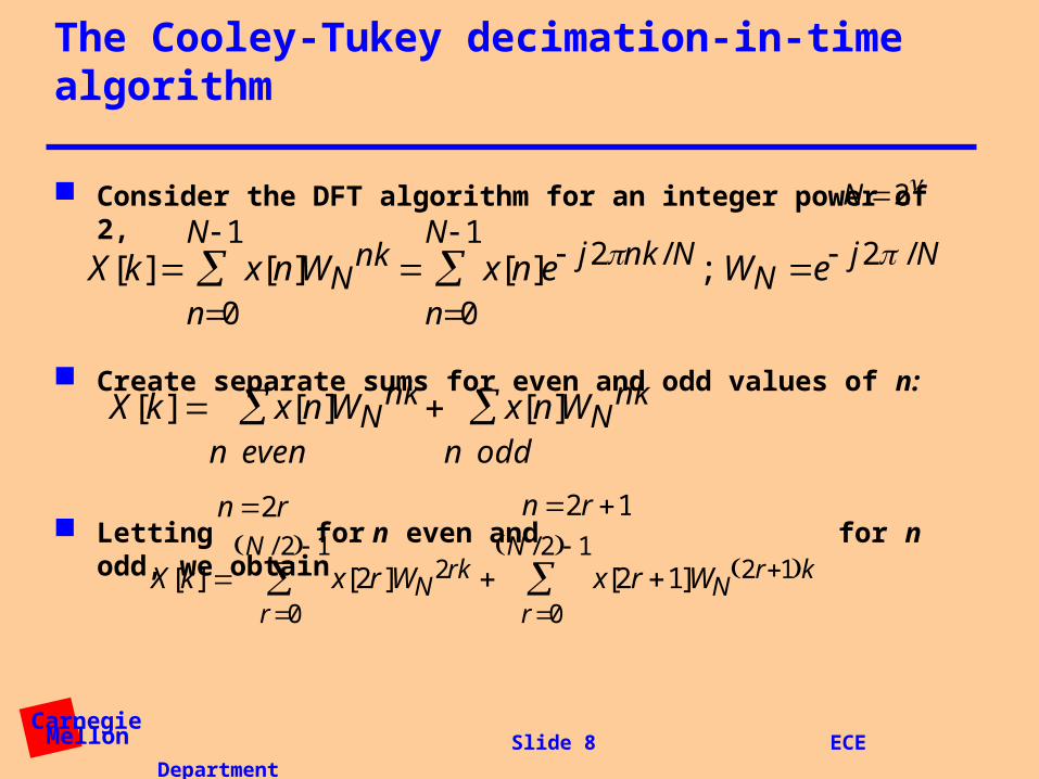
The Cooley-Tukey decimation-in-time algorithm
Consider the DFT algorithm for an integer power of 2,
Create separate sums for even and odd values of n:
Letting for n even and for n odd, we obtain
N 2
X[k]n0
N 1 x[n]WN
nk n0
N 1 x[n]e j2nk /N ; WN e j2 /N
X[k] x[n]WNnk
n even x[n]WN
nk
n odd
n 2r n 2r 1
X[k] x[2r]WN2rk
r0
N / 2 1
x[2r 1]WN2r1 k
r0
N /2 1

CarnegieMellon
Slide 9 ECE Department
The Cooley-Tukey decimation in time algorithm
Splitting indices in time, we have obtained
But and
So …
N/2-point DFT of x[2r] N/2-point DFT of x[2r+1]
X[k] x[2r]WN2rk
r0
N / 2 1
x[2r 1]WN2r1 k
r0
N /2 1
WN2 e j22 / N e j2 /(N / 2) WN / 2 WN
2rkWNk WN
kWN / 2rk
X[k] n0
(N/ 2) 1
x[2r]WN /2rk WN
k
n0
(N/ 2) 1
x[2r 1]WN / 2rk

CarnegieMellon
Slide 10 ECE Department
Savings so far …
We have split the DFT computation into two halves:
Have we gained anything? Consider the nominal number of multiplications for
– Original form produces multiplications
– New form produces multiplications
– So we’re already ahead ….. Let’s keep going!!
X[k] k0
N 1
x[n]WNnk
n0
(N/ 2) 1
x[2r]WN /2rk WN
k
n0
(N/ 2) 1
x[2r 1]WN / 2rk
N 8
2(42 ) 8 40
82 64

CarnegieMellon
Slide 11 ECE Department
Signal flowgraph notation
In generalizing this formulation, it is most convenient to adopt a graphic approach …
Signal flowgraph notation describes the three basic DSP operations:
– Addition
– Multiplication by a constant
– Delay
x[n]
y[n]x[n]+y[n]
x[n]a
ax[n]
x[n] x[n-1]z-1

CarnegieMellon
Slide 12 ECE Department
Signal flowgraph representation of 8-point DFT
Recall that the DFT is now of the form
The DFT in (partial) flowgraph notation:
X[k] G[k]WNkH[k]
CarnegieMellon
Slide 13 ECE Department
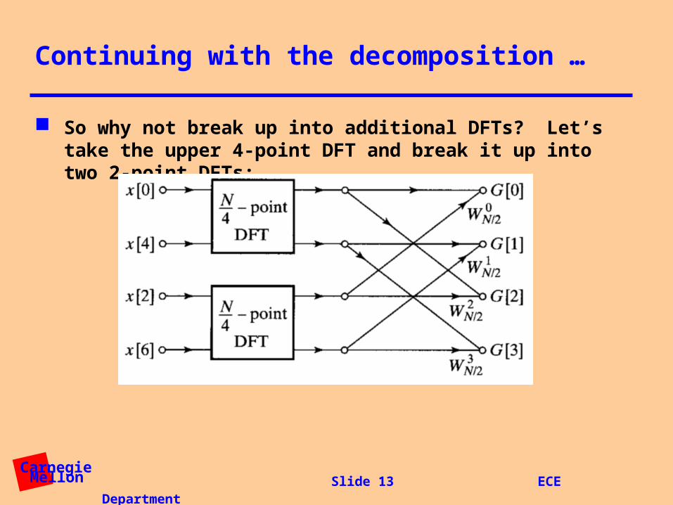
Continuing with the decomposition …
So why not break up into additional DFTs? Let’s take the upper 4-point DFT and break it up into two 2-point DFTs:

CarnegieMellon
Slide 14 ECE Department
The complete decomposition into 2-point DFTs

CarnegieMellon
Slide 15 ECE Department
Now let’s take a closer look at the 2-point DFT
The expression for the 2-point DFT is:
Evaluating for we obtain
which in signal flowgraph notation looks like ...
X[k] n0
1
x[n]W2nk
n0
1
x[n]e j2nk / 2
k 0,1
X[0] x[0] x[1]
X[1] x[0] e j21/ 2x[1] x[0] x[1]
This topology is referred to as thebasic butterfly

CarnegieMellon
Slide 16 ECE Department
The complete 8-point decimation-in-time FFT

CarnegieMellon
Slide 17 ECE Department
Number of multiplys for N-point FFTs
Let
(log2(N) columns)(N/2 butterflys/column)(2 mults/butterfly)
or ~ multiplys
N 2 where log2 (N)
N log2(N)

CarnegieMellon
Slide 18 ECE Department
“Slow” DFT requires N mults; FFT requires N log2(N) mults
Filtering using FFTs requires 3(N log2(N))+2N mults
Let
N 1 2
16 .25 .8124
32 .156 .50
64 .0935 .297
128 .055 .171
256 .031 .097
1024 .0097 .0302
Comparing processing with and without FFTs
Note: 1024-point FFTs accomplish speedups of 100for filtering, 30 for DFTs!
1 N log2 (N) / N2 ; 2 [3(N log2 (N)) N] / N 2

CarnegieMellon
Slide 19 ECE Department
Additional timesavers: reducing multiplications in the basic butterfly
As we derived it, the basic butterfly is of the form
Since we can reducing computation by 2 by premultiplying by
WNN / 2 1
WNr
WNr
WNrN / 2
WNr
1
1
CarnegieMellon
Slide 20 ECE Department
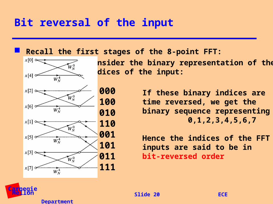
Consider the binary representation of theindices of the input:
0 0004 1002 0106 1101 0015 1013 0117 111
Bit reversal of the input
Recall the first stages of the 8-point FFT:
If these binary indices are time reversed, we get the binary sequence representing 0,1,2,3,4,5,6,7
Hence the indices of the FFTinputs are said to be in bit-reversed order
CarnegieMellon
Slide 21 ECE Department
Some comments on bit reversal
In the implementation of the FFT that we discussed, the input is bit reversed and the output is developed in natural order
Some other implementations of the FFT have the input in natural order and the output bit reversed (to be described Thursday)
In some situations it is convenient to implement filtering applications by
– Use FFTs with input in natural order, output in bit-reversed order
– Multiply frequency coefficients together (in bit-reversed order)
– Use inverse FFTs with input in bit-reversed order, output in natural order
Computing in this fashion means we never have to compute bit reversal explicitly

CarnegieMellon
Slide 22 ECE Department
Summary
We developed the structure of the basic decimation-in-time FFT
Use of the FFT algorithm reduces the number of multiplys required to perform the DFT by a factor of more than 100 for 1024-point DFTs, with the advantage increasing with increasing DFT size
Next time we will consider inverse FFTs, alternate forms of the FFT, and FFTs for values of DFT sizes that are not an integer power of 2
Recommended


![[1905] 2 K.B. 791](https://img.pdfslide.us/doc/110x75/577d20bf1a28ab4e1e93aa5a/1905-2-kb-791.jpg)