Slide 1
18-660: Numerical Methods for Engineering Design and Optimization
Xin Li Department of ECE
Carnegie Mellon University Pittsburgh, PA 15213

Slide 2
Overview
Conjugate Gradient Method (Part 4) Pre-conditioning Nonlinear conjugate gradient method

Slide 3
Conjugate Gradient Method
Step 1: start from an initial guess X(0), and set k = 0
Step 2: calculate
Step 3: update solution
Step 4: calculate residual
Step 5: determine search direction
Step 6: set k = k + 1 and go to Step 3
( ) ( ) ( ) ( ) ( )( ) ( )
( ) ( )kTk
kTkkkkkk
ADDRDDXX =+=+ µµ where1
( ) ( ) ( )000 AXBRD −==
( ) ( ) ( ) ( )kkkk ADRR µ−=+1
( ) ( ) ( )( ) ( )
( ) ( )kTk
kTk
kkk
kkkk
RDRRDRD
11
,1,111 where
++
++++ =+= ββ

Slide 4
Convergence Rate
Conjugate gradient method has slow convergence if κ(A) is large I.e., AX = B is ill-conditioned
In this case, we want to improve convergence rate by pre-
conditioning
( ) ( )( )
( ) XXAA
XXk
k −⋅
+−
≤−+ 01
11
κκ
Slide 5
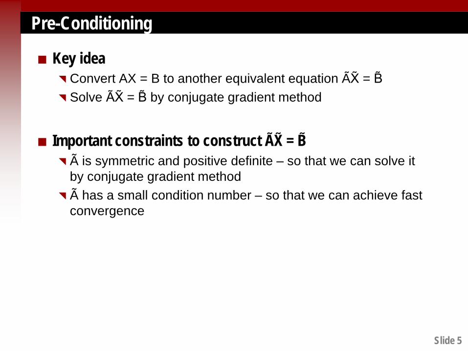
Pre-Conditioning
Key idea Convert AX = B to another equivalent equation AX = B Solve ÃX = B by conjugate gradient method
Important constraints to construct AX = B
à is symmetric and positive definite – so that we can solve it by conjugate gradient method
à has a small condition number – so that we can achieve fast convergence
Slide 6
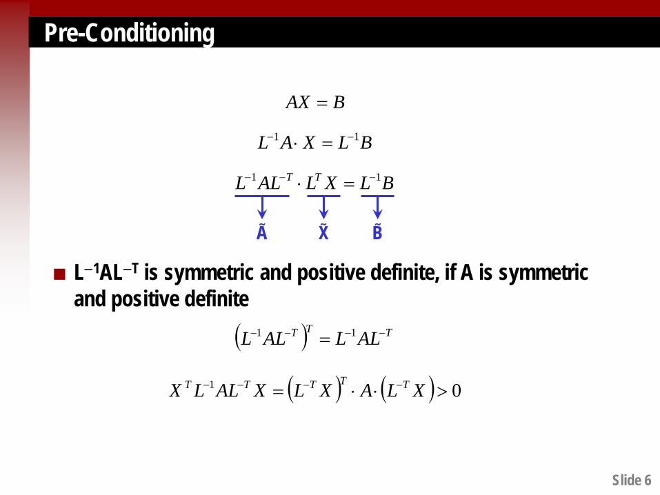
Pre-Conditioning
L−1AL−T is symmetric and positive definite, if A is symmetric and positive definite
BAX =
BLXLALL TT 11 −−− =⋅
BLXAL 11 −− =⋅
A X B
( ) TTT ALLALL −−−− = 11
( ) ( ) 01 >⋅⋅= −−−− XLAXLXALLX TTTTT
Slide 7
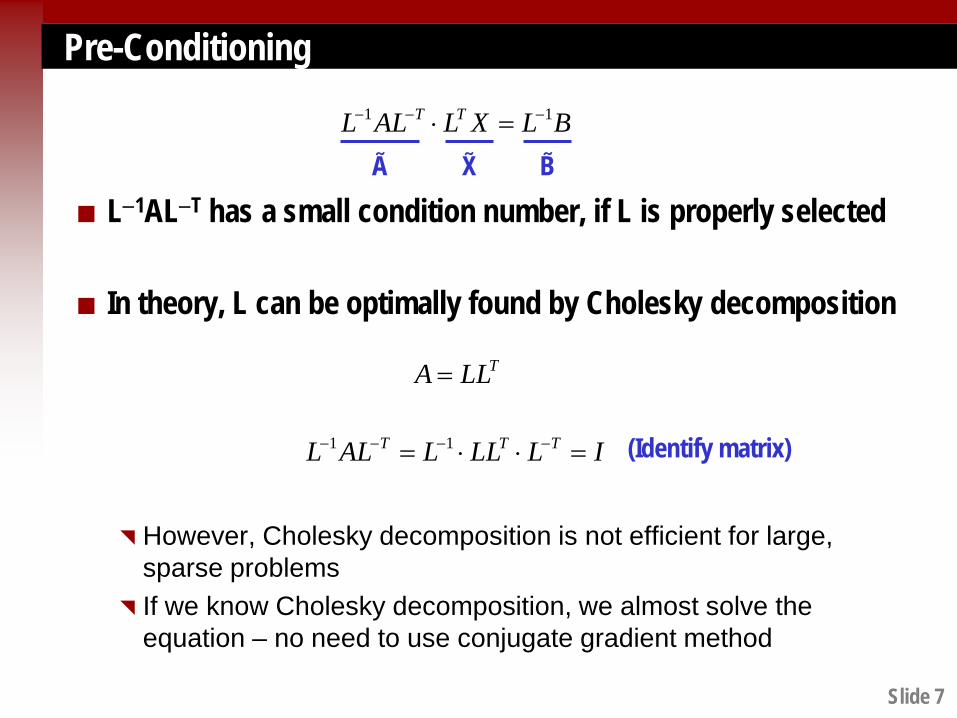
Pre-Conditioning
L−1AL−T has a small condition number, if L is properly selected
In theory, L can be optimally found by Cholesky decomposition
However, Cholesky decomposition is not efficient for large, sparse problems
If we know Cholesky decomposition, we almost solve the equation – no need to use conjugate gradient method
TLLA =
ILLLLALL TTT =⋅⋅= −−−− 11 (Identify matrix)
BLXLALL TT 11 −−− =⋅
A X B
Slide 8
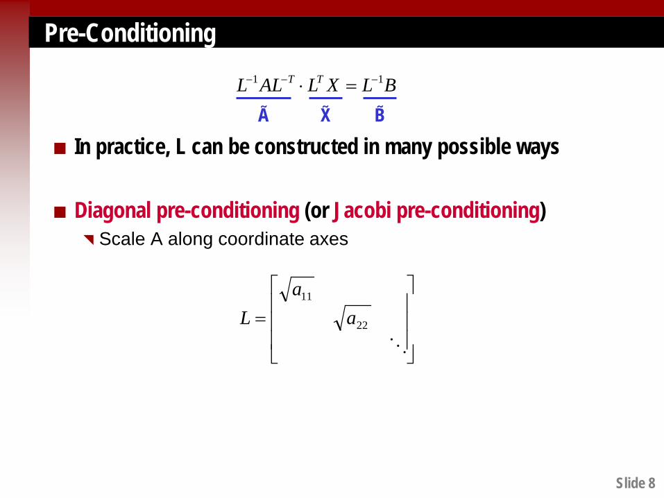
Pre-Conditioning
In practice, L can be constructed in many possible ways
Diagonal pre-conditioning (or Jacobi pre-conditioning) Scale A along coordinate axes
=
22
11
aa
L
BLXLALL TT 11 −−− =⋅
A X B
Slide 9
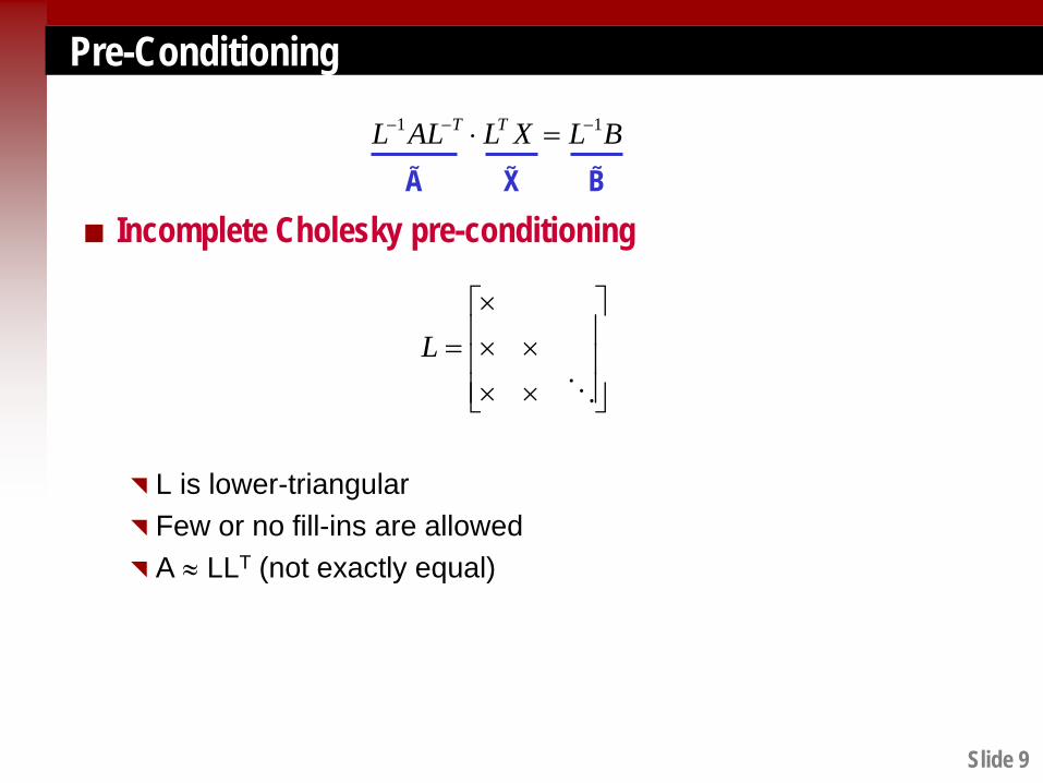
Pre-Conditioning
Incomplete Cholesky pre-conditioning
L is lower-triangular Few or no fill-ins are allowed A ≈ LLT (not exactly equal)
××××
×=
L
BLXLALL TT 11 −−− =⋅
A X B

Slide 10
Pre-Conditioning
Step 1: start from an initial guess X(0), and set k = 0
Step 2: calculate
Step 3: update solution
Step 4: calculate residual
Step 5: determine search direction
Step 6: set k = k + 1 and go to Step 3
( ) ( ) ( ) ( ) ( )( ) ( )
( ) ( )kTTk
kTkkkkkk
DALLDRDDXX ~~~~
~where~~~~1
1−−
+ =+= µµ
( ) ( ) ( )01100 ~~~ XALLBLRD T−−− −==
( ) ( ) ( ) ( )kTkkk DALLRR ~~~~ 11 −−+ −= µ
( ) ( ) ( )( ) ( )
( ) ( )kTk
kTk
kkk
kkkk
RDRRDRD ~~~~~where~~~~ 11
,1,111
++
++++ =+= ββ

Slide 11
Pre-Conditioning
L−1 should not be explicitly computed Instead, Y = L−1W or Y = L−TW (where W is a vector) should be
computed by solving linear equation LY = W or LTY = W
( ) ( ) ( ) ( ) ( )( ) ( )
( ) ( )kTTk
kTkkkkkk
DALLDRDDXX ~~~~
~where~~~~1
1−−
+ =+= µµ
( ) ( ) ( ) ( )kTkkk DALLRR ~~~~ 11 −−+ −= µ
( ) ( ) ( )( ) ( )
( ) ( )kTk
kTk
kkk
kkkk
RDRRDRD ~~~~~where~~~~ 11
,1,111
++
++++ =+= ββ
BLXLALL TT 11 −−− =⋅
A X B
( ) ( ) ( )01100 ~~~ XALLBLRD T−−− −==

Slide 12
Pre-Conditioning
Diagonal pre-conditioning L is a diagonal matrix Y = L−1W or Y = L−TW can be found by simply scaling
=
⋅
WYaa
22
11
2222
1111
awy
awy
=
=

Slide 13
Pre-Conditioning
Incomplete Cholesky pre-conditioning L is lower-triangular Y = L−1W or Y = L−TW can be found by backward substitution
=
⋅
WY
llll
l
3231
2221
11
( )
2212122
1111
lylwylwy
−==

Slide 14
Pre-Conditioning
Once X is known, X is calculated as X = L−TX Solve linear equation L−TX = X by backward substitution
BLXLALL TT 11 −−− =⋅
A X B
=
⋅
XXll
lll~
3222
312111
( )
1,11,11~
~
−−−−− −==
NNNNNNN
NNNN
lxlxxlxx
=
⋅
XXaa
~000
22
11
2222
1111
~
~
axx
axx
=
=
Diagonal pre-conditioning Incomplete Cholesky pre-conditioning

Slide 15
Nonlinear Conjugate Gradient Method
Conjugate gradient method can be extended to general (i.e., non-quadratic) unconstrained nonlinear optimization
A number of changes must be made to solve nonlinear optimization problems
CXBAXX TT
X+−
21min
BAX 1−=
Quadratic programming
Nonlinear programming
( )XfX
min
Slide 16
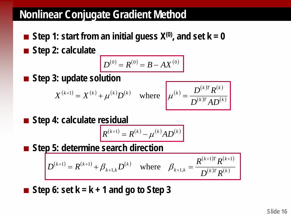
Nonlinear Conjugate Gradient Method
Step 1: start from an initial guess X(0), and set k = 0
Step 2: calculate
Step 3: update solution
Step 4: calculate residual
Step 5: determine search direction
Step 6: set k = k + 1 and go to Step 3
( ) ( ) ( ) ( ) ( )( ) ( )
( ) ( )kTk
kTkkkkkk
ADDRDDXX =+=+ µµ where1
( ) ( ) ( )000 AXBRD −==
( ) ( ) ( ) ( )kkkk ADRR µ−=+1
( ) ( ) ( )( ) ( )
( ) ( )kTk
kTk
kkk
kkkk
RDRRDRD
11
,1,111 where
++
++++ =+= ββ

Slide 17
Nonlinear Conjugate Gradient Method
New definition of residual
“Residual” is defined by the gradient of f(X) If X* is optimal, ∇f(X*) = 0 −∇f(X*) = B − AX for quadratic programming
( ) ( ) ( )
( ) ( ) ( ) ( )kkkk ADRRAXBRD
µ−=
−==+1
000
Quadratic programming Nonlinear programming
( ) ( )[ ]kk XfR −∇=

Slide 18
Nonlinear Conjugate Gradient Method
New formula for conjugate search directions
Ideally, search directions should be computed by Gram-Schmidt conjugation of residues In practice, we often use approximate formulas
( ) ( )
( ) ( )kTk
kTk
kk RRRR 11
,1
++
+ =β
Quadratic programming
( ) ( ) ( )( ) ( )
( ) ( )kTk
kTk
kkk
kkkk
RDRRDRD
11
,1,111 where
++
++++ =+= ββ
( ) ( ) ( )[ ]( ) ( )kTk
kkTk
kk RRRRR −⋅
=++
+
11
,1β
Fletcher-Reeves formula Polak-Ribiere formula
Slide 19
Nonlinear Conjugate Gradient Method
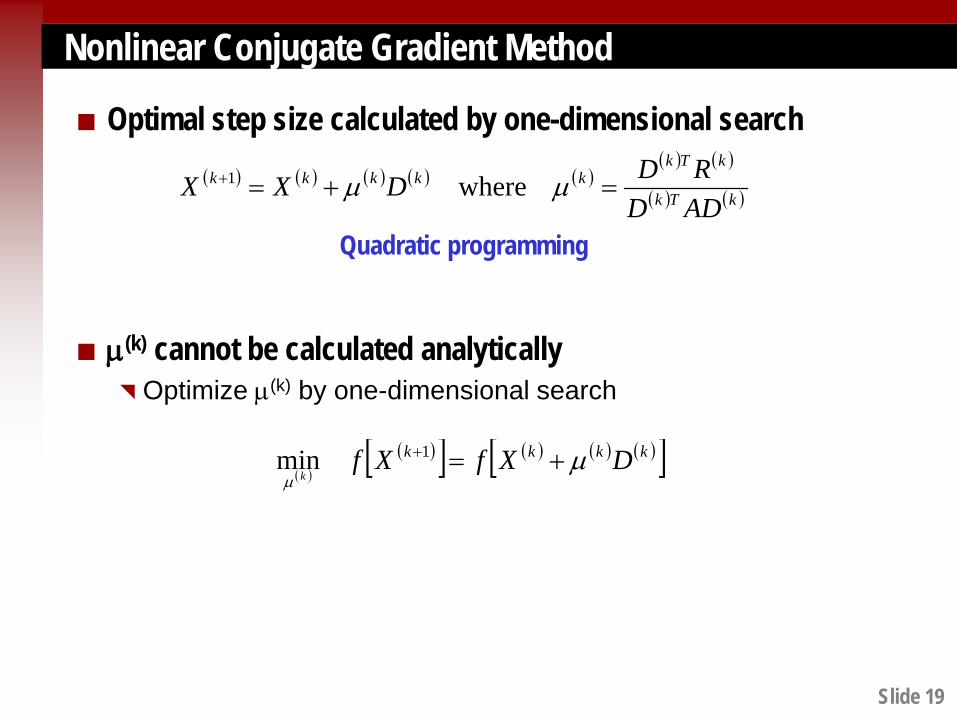
Optimal step size calculated by one-dimensional search
µ(k) cannot be calculated analytically Optimize µ(k) by one-dimensional search
( ) ( ) ( ) ( ) ( )( ) ( )
( ) ( )kTk
kTkkkkkk
ADDRDDXX =+=+ µµ where1
Quadratic programming
( )( )[ ] ( ) ( ) ( )[ ]kkkk DXfXf
kµ
µ+=+1min
Slide 20
Nonlinear Conjugate Gradient Method
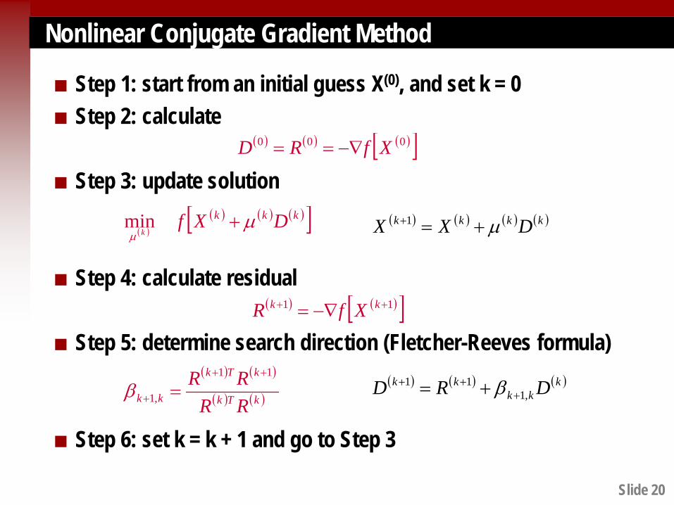
Step 1: start from an initial guess X(0), and set k = 0
Step 2: calculate
Step 3: update solution
Step 4: calculate residual
Step 5: determine search direction (Fletcher-Reeves formula)
Step 6: set k = k + 1 and go to Step 3
( ) ( ) ( ) ( )kkkk DXX µ+=+1
( ) ( ) ( )[ ]000 XfRD −∇==
( ) ( )[ ]11 ++ −∇= kk XfR
( ) ( ) ( )kkk
kk DRD ,111
+++ += β
( )( ) ( ) ( )[ ]kkk DXf
kµ
µ+min
( ) ( )
( ) ( )kTk
kTk
kk RRRR 11
,1
++
+ =β

Slide 21
Nonlinear Conjugate Gradient Method
Gradient method, conjugate gradient method and Newton method Conjugate gradient method is often preferred for many practical
large-scale engineering problems
Gradient Conjugate Gradient Newton
1st-Order Derivative Yes Yes Yes 2nd-Order Derivative No No Yes
Pre-conditioning No Yes No Cost per Iteration Low Low High Convergence Rate Slow Fast Fast
Preferred Problem Size Large Large Small

Slide 22
Summary
Conjugate gradient method (Part 4) Pre-conditioning Nonlinear conjugate gradient method
Recommended