1
The 4 standard failure models
-to be used in maintenance optimization, with focus on state modelling
Professor Jørn Vatn

2
Situations and maintenance tasks
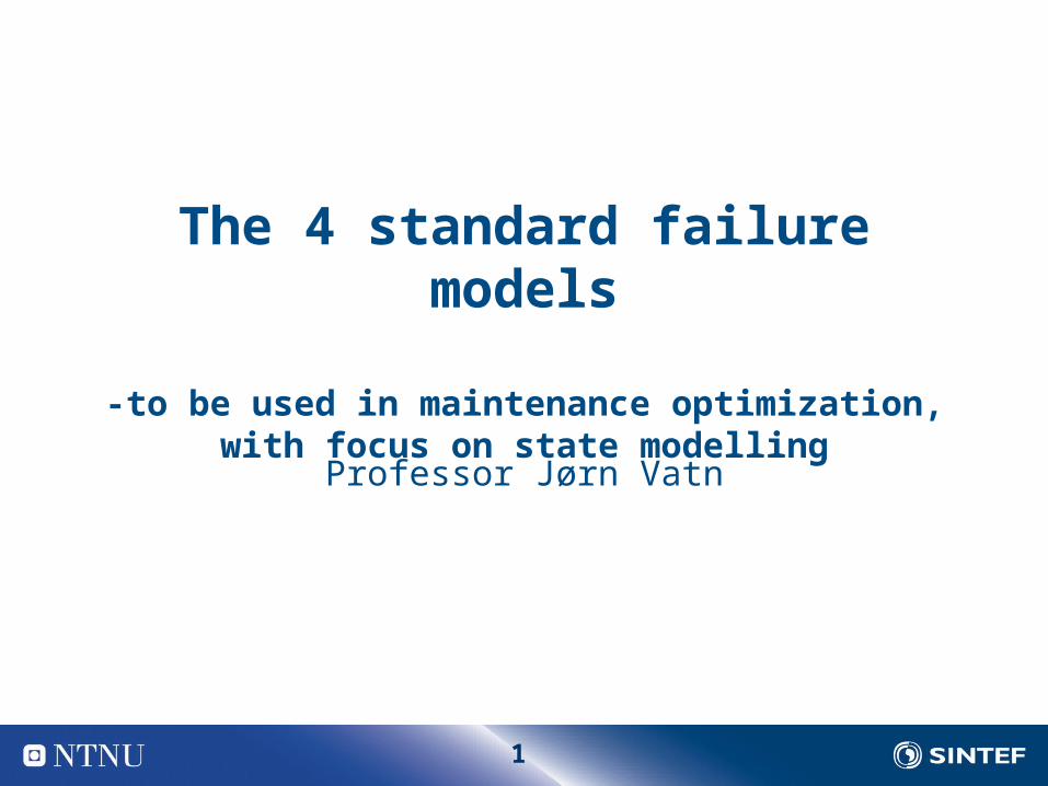
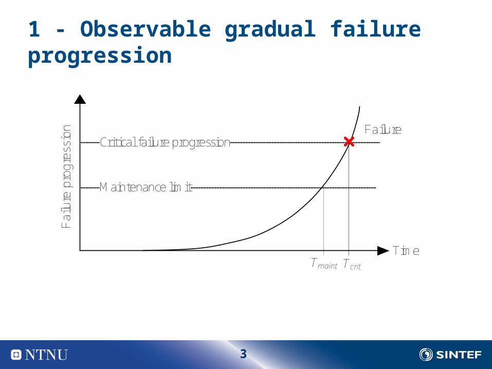
1. Observable gradual failure progression Inspect at regular intervals (or with shorter and shorter intervals) Replace when degradation is high
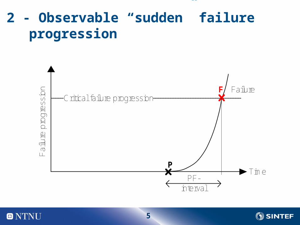
2. Observable “sudden” failure progression Inspect at regular intervals Replace if failure progression is detected
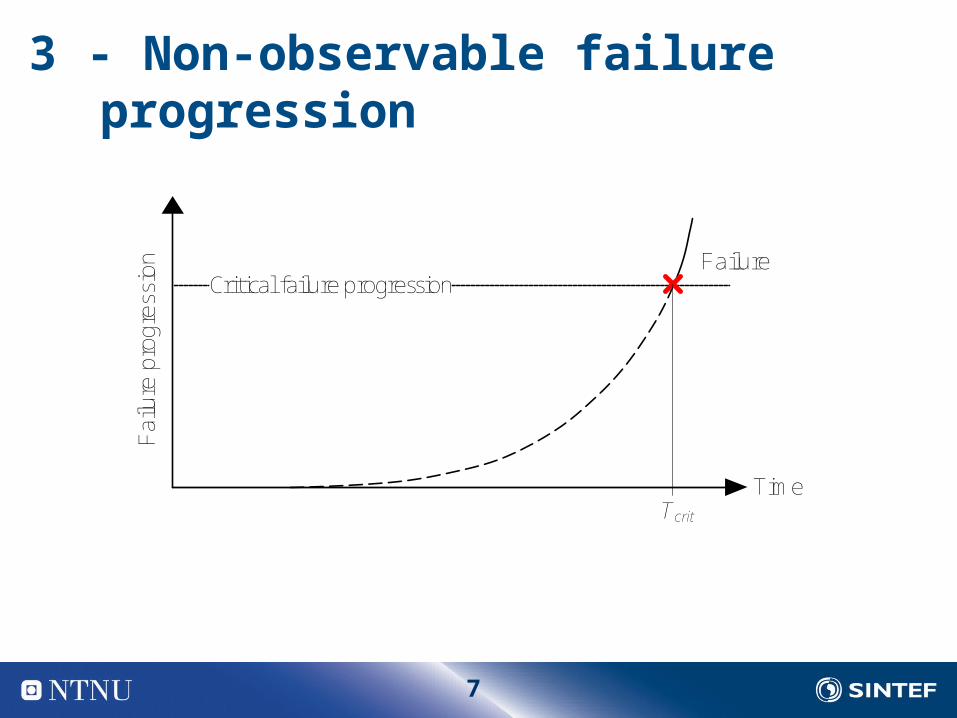
3. Non-observable failure progression Replace based on age
4. Shock Perform functional test to identify hidden failures
3
1 - Observable gradual failure progression F
ailu
re p
rogr
essi
on
TimeTcrit
Failure
Tmaint
Critical failure progression
Maintenance limit
4
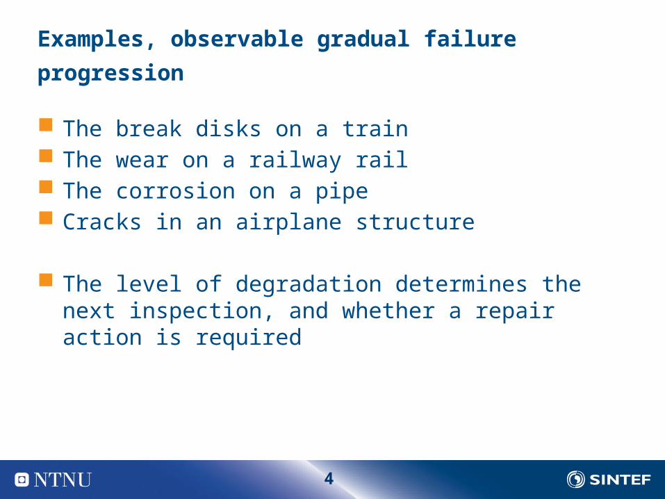
Examples, observable gradual failure progression
The break disks on a train The wear on a railway rail The corrosion on a pipe Cracks in an airplane structure
The level of degradation determines the next inspection, and whether a repair action is required
5
2 - Observable “sudden” failure progressionF
ailu
re p
rog
ress
ion
Time
FailureCritical failure progression
F
P
PF- interval

6
Examples: observable “sudden” failure progression
Cracks in a train wheel Isolation resistance in a signalling cable
7
3 - Non-observable failure progressionF
ailu
re p
rogr
essi
on
TimeTcrit
FailureCritical failure progression

8
4 - ShockF
ailu
re p
rogr
essi
on
Time
FailureCritical failure progression
F
P

9
Multistate systems
Multistate systems are described by performance measures
We use a state variable, Y(t), to describe the state of the system at time t, e.g., Performance (pump capacity, compressor efficiency etc)
For binary systems Y(t) reduces to take only the values 0 and 1; Y(t) = 1 represents a functioning state, and Y(t) = 0 represents a fault state
Y(t) is a random quantity, i.e. expressed in probabilistic terms, involving model parameters

10
Content of the state variable Y(t)
Y(t) was introduced as a performance variable However, we will let Y(t) be more general, and Y(t) will be
used to express the state of the system at time t, i.e.; the direct performance of the system, capacities etc., or a direct measure of wear, or an indication of wear or increased failure probability
We use W(t) as a general quantity that simply is related to degradation of the system:

11
Degradation quantities of interest
WP(t): Quantities that are direct performance measures ($!!!) E.g., the pumping capacity of a pump
WI(t): Quantities that are only indicators of the degradation of the component E.g., the bearing temperature
WD(t): Quantities that represent measurable degradation Examples are crack shape and size, corrosion level, geometrical defects
(inclusive wear)
WS(t): Stressors that influence the degradation process Examples could be the cyclic loads and corrosive medium The stressors them selves do not measure the likelihood of failure, but is
important for the forecasting of the failure progression
WP(t), WI(t) and WD(t) will be (probabilistic) modelled by the state variable Y(t)
12
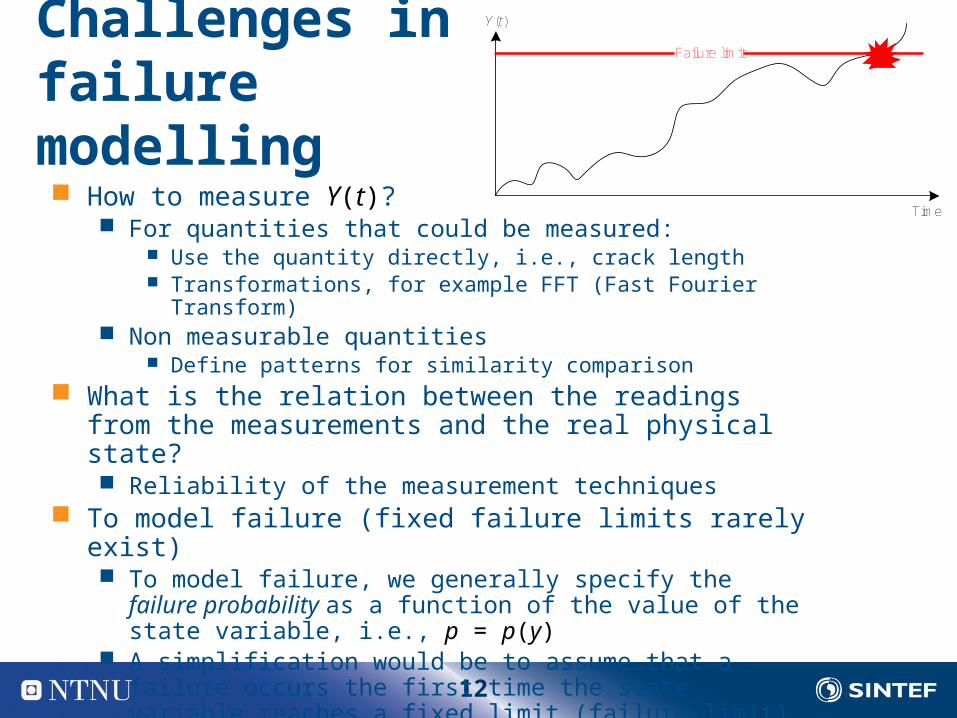
Challenges in failure modelling How to measure Y(t)?
For quantities that could be measured: Use the quantity directly, i.e., crack length Transformations, for example FFT (Fast Fourier Transform)
Non measurable quantities Define patterns for similarity comparison
What is the relation between the readings from the measurements and the real physical state? Reliability of the measurement techniques
To model failure (fixed failure limits rarely exist) To model failure, we generally specify the failure probability as a
function of the value of the state variable, i.e., p = p(y) A simplification would be to assume that a failure occurs the first
time the state variable reaches a fixed limit (failure limit)
Time
Y(t)
Failure limit

13
Purpose of modelling – binary systems
We want to establish a mathematical model describing the relation between the effective failure rate, E, and the maintenance, i.e.,
the inspection interval, , and the intervention level, l
E = E(,l) Establish a cost model:
PM cost (inspection interval)-1
Renewal cost increases with a restrictive intervention level CM cost/unavailability cost increases with increasing inspection interval CM cost/unavailability cost decreases with a restrictive intervention level
Example
lE(t,l)
t
l=6l=3

14
Classes of probabilistic models used PF model
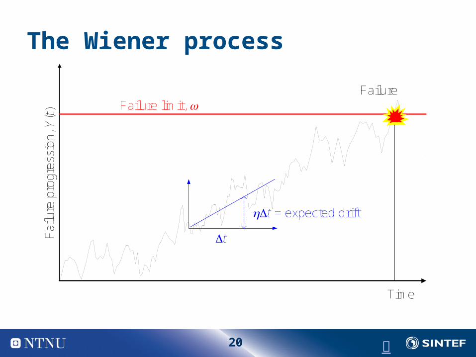
Failure progression is defined between a potential failure (P) and a failure (F) The Wiener process
During an arbritary time interval t, the “failure progression” is increased by a normally distributed quantity with mean t and variance
2t A failure occurs the first time the failure progression passes the critical value
The Gamma process Similar to the Wiener process, but the increments are gamma distributed
The shock model The system is exposed to shocks, and each shock causes a damage Xi
When the accumulated damage increases, so does also the failure probability The Markov state model
The failure progression is approximated by a discrete set of states The transitions between the sates are assumed to follow a Markov process The model is very flexible, and allows for modeling a large range of situations
Markov model
15
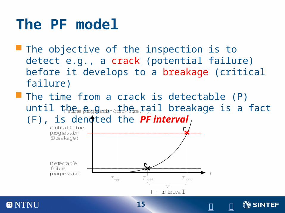
The PF model
The objective of the inspection is to detect e.g., a crack (potential failure) before it develops to a breakage (critical failure)
The time from a crack is detectable (P) until the e.g., the rail breakage is a fact (F), is denoted the PF interval
Failure progression/crack size, Y(t)
PF interval
t
Critical failureprogression(Breakage)
Detectablefailureprogression
Tinit T critT det
P
F
16
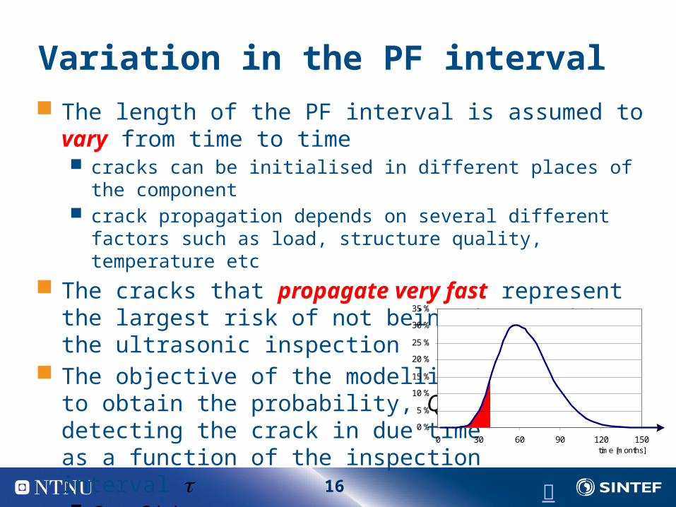
Variation in the PF interval The length of the PF interval is assumed to vary from time
to time cracks can be initialised in different places of the component crack propagation depends on several different factors such as
load, structure quality, temperature etc
The cracks that propagate very fast represent the largest risk of not being detected by the ultrasonic inspection
The objective of the modelling isto obtain the probability, Q, of notdetecting the crack in due timeas a function of the inspectioninterval Q = Q()
0 %
5 %
10 %
15 %
20 %
25 %
30 %
35 %
0 30 60 90 120 150time [months]

17
Determining Q0 (simplified)
TPF PF interval (random variable)
PF Probability distribution function of TPF
q Failure probability of one inspection Inspection interval
Qt Failure probability for fixed value, TPF = t
Q0 Failure probability of given strategy

18
The argument Assume PF-interval is fixed, i.e., TPF = t
Let n = int(t/) Number of opportunities for inspection:
We get an extra inspection, if the first inspection after the «P» comes before time units, i.e.,
Probability of n+1 opportunities:
P Ft
Best t t t t t t n + 1 opportunities
Worst t t t t t t n opportunities
D
19
Cost elements - Optimization
The most important cost elements are: The cost per inspection, CI The (unavailability) cost per system failure, CF The cost of repairing a system failure, CCM The cost of renewing the system upon a potential failure, CRC
The total cost per unit time is then
C() = CI/ + (CF+CCM)E() + CRC()
The objective is now to minimize C() wrt maintenance interval and intervention level E() Q0 / (MTTF-E(TPF) ) E() (1-Q0 )/ (MTTF-E(TPF) ) = renewal rate
20
The Wiener process
Failure
Time
Fai
lure
pro
gres
sion
, Y(t
) Failure limit,
Dt
hDt = expected drift

21
The shock model
Failure
Time
Acc
umul
ated
dam
age,
Y(t
)
ith shock
Xi damage caused by ith shock
The shocks represent WS(t)
The magnitude of the shock also represents WS(t)
The impact Xi represents WD(t)
22
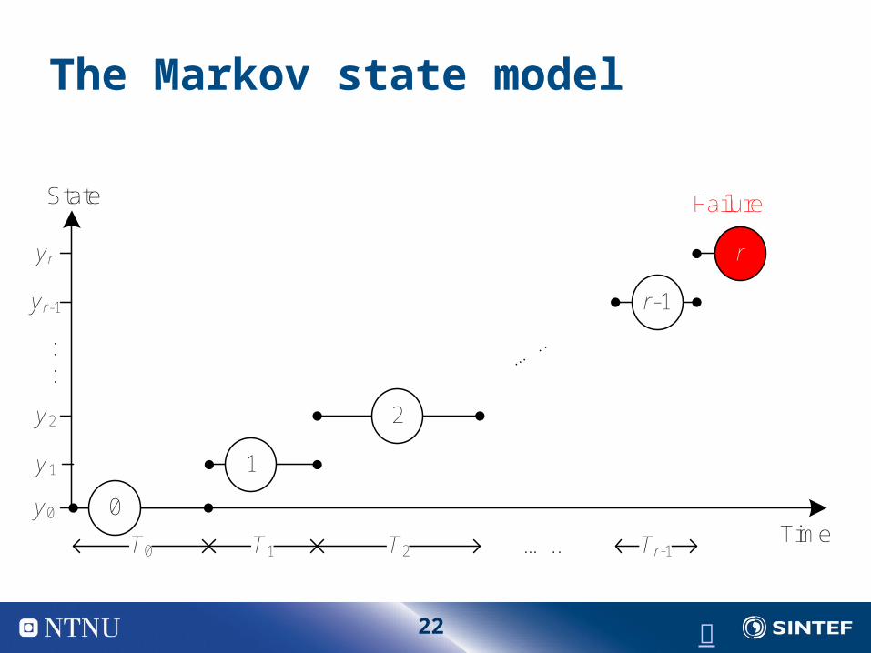
The Markov state model
y1
y2
yr-1
yr
1
2
r
r-1
T1 T2 Tr-1Time
State
y0 0
T0 …..
::
Failure
…..

23
Model assumptions
The state variable, Y(t), describes the state of the system at time t, Y(t) is a random quantity
The state variable could take one of the values y0, y1,…, yr
The values could either be numerical, or a qualitative description of a state or phenomenon
The system starts in state y0, and jumps to a higher state (yi to yi+1) with a time independent intensity i
There is generally a cost assossiated with being in state yi
The system fault state is yr
The system is inspected at intervals of length (offline) The system is renewed if Y(t) yl at an inspection
y1
y2
yr
1
2
r
State
y0 0
::
t

24
Maintenance
y1
y2
yl
yr
1
2
r
l
Timet
y0 0
::
Maintenance limit
3t2t 4t 5t 6t 8t7t
l0
l r-1
l1
CalculationPar. Spec.

25
Markov differential equations
Introduce Pi(t) = Pr(the system is in state i at time t)
Consider the change in a small time interval t: Standard Markov considerations gives:
Pi(t+t) = Pi(t)(1-it) + Pi-1(t) i-1t (*)
Equation (*) could now be used to obtain the state probabilities, Pi(t), as a function of time by numerical integration
i
r
li-1
i-1
li

26
The easy situation: no maintenance
If no maintenance is carried out then integrate equation (*) starting from the initial state
Mean time to failure is given by: MTTF = t=0: R(t) dt = t=0: [1-Pr(t)]dt in fact a sum …
To verify our calculations we should verify the analytical result: MTTF = i=0:r-1MTTFi = i=0:r-11/i

27
Calculation procedure: with maintenance
The system is inspected at intervals of length The system is renewed if Y(t) yl at an inspection (Fig.)
The model is integrated as before, but when t equals , 2, 3,… special considerations are necessary
Procedure1. Define the initial conditions: P0(0) = 1, Pi(0) = 1, i > 0
2. Set f = 0, t = 0, t = sufficient small
3. Integrate Equation (*) one step, and let t = t + t4. Let f = f + Pr(t)
5. If t =, 2, 3,…, then let P0(t) = P0(t)+ il Pi(t), and Pi(t) = 0, il
6. Loop to Step 3 until t is sufficient large
7. System failure frequency now equals E(,l) = f/t

28
Do While t < MaxT ‘ Main loop
nFail = nFail + IntegrateDt(dt)
P(0) = P(0) + P(r)
P(r) = 0
t = t + dt
If t > inspection Then
inspection = inspection + tau
nRenewal = nRenewal + Inspect(L, q)
End If
Loop
Function IntegrateDt(dt As Single)
For i = r To 1 Step -1
P(i) = P(i) * (1 - lam (i) * dt) _
+ P(i - 1) * lam (i - 1) * dt
Next
P(0) = P(0) * (1# - lambda(0) * dt)
IntegrateDt = P(r)
End Function
Function Inspect(L As Integer, q As Single)
rr = 0
For i = L To r - 1
rr = rr + P(i) * (1 - q)
P(0) = P(0) + P(i) * (1 - q)
P(i) = P(i) * q
Next i
DoInsp = rr
End Function
Essential source code in VBA

29
Specification of model parameters
In principle we need to specify all transition rates, i.e. 0, 1,…, r-1
We also need the probability of erroneous classification Qij = Pr(Classify into state i when the real state is j)
In order to get numerical values (estimates) of the model parameters, we utilise: Experience data Expert and engineering judgements Degradation modelling, i.e. fracture mechanics, FEM etc
For r > 4-5 this will be a huge number of parameters We want to simplify the parameter specification procedure

30
Simplified parameter specification
We specify the parameters in the situation without maintenance, i.e. What will the mean time to failure (MTTF) be if no maintenance is
carried out? (Fig. ) Is the transition rate between states constant, or increasing?
If it is increasing then we specify the ratio: V = r-1/0 = how much faster failure progression is just before failure
compared to initially (Fig. )
We also need to specify The number of states in the model (r ) The probability q that an inspection does not reveal that the
system is in a critical state
Calculation example

31
MTTF without maintenance
y1
y2
yr-1
yr
1
2
r
r-1
Timey0 0
::
Failure
…..
MTTF without maintenance

32
Calculation example
Input parameters: Result
MarkovStateModel.xls
Input values MTTF 120 r 8
V=lr-1/l0 8 t 12 Intervention, l 4 q 0,05 Time horizon 4800
Output result v 1,35
l0 0,0294 MTTF-verify 119,98 MTTF(t,l) 2480,14
lA(tl) 0,00040 Ren. Rate 0,01008 MTBR 99,25

33
The effect of maintenance
We have established (by means of the Excel model) the relation between maintenance ( and l) and i) the effective failure rate, E(,l), and ii) the renewal rate (,l)
Example resultsEffective failure rate, lE(t,l)
0
0,001
0,002
0,003
0,004
0,005
0,006
3 6 9 12 15 18 21 24
Inspection interval, t
Intervention: l = 6
Intervention: l = 4

34
Cost elements - Optimization
The most important cost elements are: The cost per inspection, CI The (unavailability) cost per system failure, CF The cost of repairing a system failure, CCM The cost of renewing the system at state l, CRC
The total cost per unit time is then
C(,l) = CI/ + (CF+CCM)E(,l) + CRC(,l)
The objective is now to minimize C(,l) wrt maintenance interval and intervention level

35
Extension of the Markov model
More advanced maintenance strategies could be applied Reducing inspection interval as we approach the maintenance
limit, l Conduct non perfect repair before the maintenance limit
Models have been developed for hydro power plant

36
The gamma process
Stationary gamma process Background: X is said to be gamma distributed with shape
parameter v, and scale parameter u if the PDF is given by: Ga(x|v,u)=uvxv-1e-ux/(v) Let Y(t) be the degradation level at time t Y(t) follows a stationary gamma process if
Y(0) = 0 Y(s) - Y(t) ~ Ga([s-t ]v,u), s>t Y(t) has independent increments

37
Mean time to failure in the gamma process
Assume that the component fails as soon as the failure progression exceeds the value
Let T denote the time to failure It follows that
FT(t) = Pr(T<t) = Pr(Y(t) > ) = (vt, u)/(vt) Where (a, x) is the incomplete gamma function
Welte (2008) reports the following: E(T) u/v + 1/(2v) Var(T) u/v2 - 1/(12v2)

38
Non-stationary gamma process
The gamma process could be extended to a non-stationary process by letting the shape parameter be a function of time, i.e., v(t) is the shape function, and we have: Y(0) = 0 Y(s) - Y(t) ~ Ga(v(s)-v(t),u), s>t Y(t) has independent increments
The CDF now readsFT(t) = Pr(T<t) = Pr(Y(t) > ) = (v(t), u)/(v(t))
The expected time to failure, and variance in time to failure could be found by numerical methods
39
Comparison – Discrete model, vs gamma process
For the discrete model we need to fix the number of states If the degradation is continuous, this seems not very
natural, hence a gamma process is more appealing Degradation rate
In the discrete model, the degradation rate (in terms of transition rates) depends on the state of the system, and not on the age (time)
In a gamma process the degradation rate could also be modelled by a non-constant value, but degradation rate depends on the age, and not on the state

40
Exercise
Verify E(T) u/v + 1/(2v) by numerical integration, i.e., E(T) = 0
R(t)dt

41
Non-stationary gamma process
The gamma process could be extended to a non-stationary process by letting the shape parameter be a function of time, i.e., v(t) is the shape function, and we have: Y(0) = 0 Y(s) - Y(t) ~ Ga(v(s)-v(t),u), s>t Y(t) has independent increments
The CDF now readsFT(t) = Pr(T<t) = Pr(Y(t) > ) = (v(t), u)/(v(t))
The expected time to failure, and variance in time to failure could be found by numerical methods

42
Integration of the gamma process
Let S|t,dt = Y(t+dt) - Y(t) be the degradation during a small time interval dt after time t
S|t,dt ~ Ga(v(t+dt)-v(t),u) Further, let g(s | t, dt) denote the pdf of S|t,dt If the pdf of Y(t) is known, we may obtain the pdf of Y(t+dt) by a
convolution argument: (*)
Assume the system is inspected every time unit, and renewed whenever Y > yM
To find the effective failure rate, we integrate (*) from t = 0 to , and whenever t = k, probability mass is moved to 0
Recommended