1
Chapter 6
CPU Scheduling

2
Chapter 6: CPU Scheduling
• Basic Concepts• Scheduling Criteria • Scheduling Algorithms• Multiple-Processor Scheduling• Real-Time Scheduling• Algorithm Evaluation
3
Basic Concepts
• The objective of multiprogramming is to maximum CPU utilization
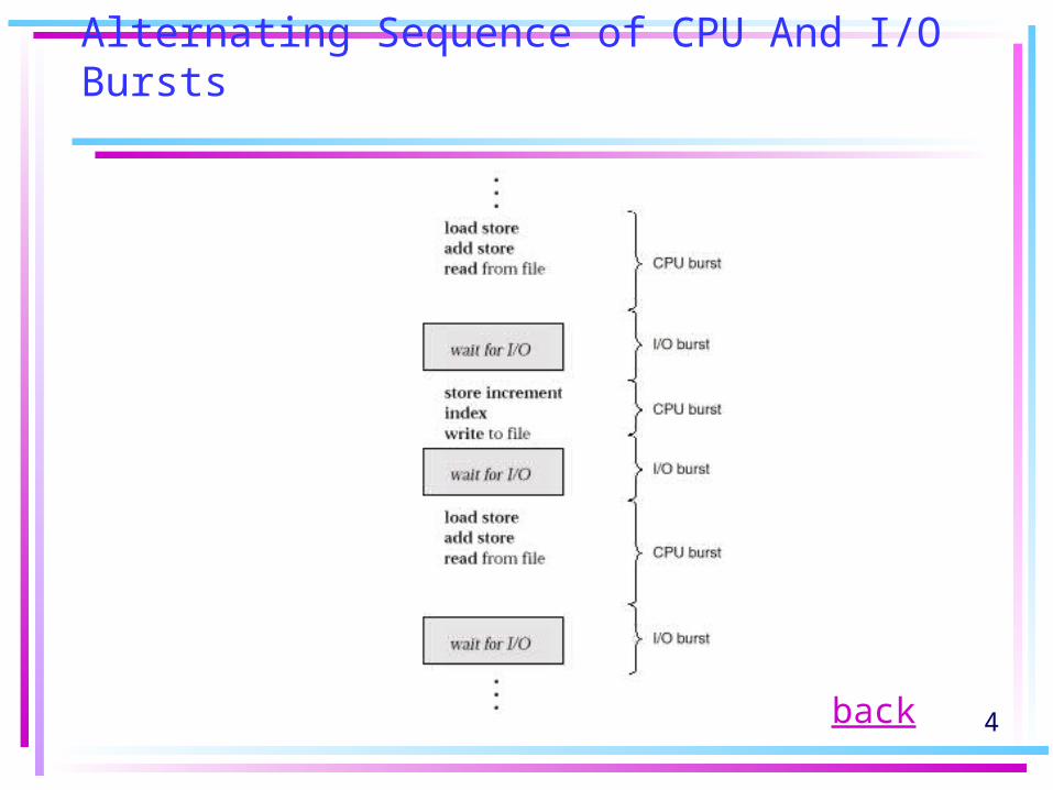
• CPU–I/O Burst Cycle – Process execution consists of a cycle of CPU execution and I/O wait. (Fig. 6.1)
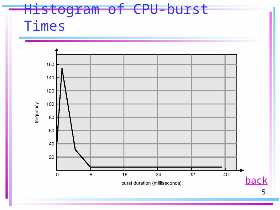
• CPU burst distribution: a large number of short CPU bursts, and a small number of long CPU bursts. (Fig. 6.2)
• An I/O-bound program typically will have many short CPU bursts. A CPU-bound program might have a few long CPU bursts.
§ 6.1
continue
爆裂
束縛,趨勢
4
Alternating Sequence of CPU And I/O Bursts
back
5
Histogram of CPU-burst Times
back
6
CPU Scheduler
• When CPU becomes idle, OS must selects from among the processes in memory that are ready to execute, and allocates the CPU to one of them.
• CPU scheduling decisions may take place when a process:1. Switches from running to waiting state.2. Switches from running to ready state.3. Switches from waiting to ready.4. Terminates.
§ 6.1.2
7
Preemptive Scheduling
• Under nonpreemptive scheduling, once the CPU has been allocated to a process, the process keeps the CPU until it releases the CPU either by terminating or by switching to the waiting state.
• Scheduling takes place only under 1 and 4 is nonpreemptive or cooperative, otherwise, it is preemptive.
• Certain hardware platform can use cooperative scheduling only, because it does not equipped with the special hardware (ex: timer).
§ 6.1.3先佔
8
Preemptive Scheduling
• Nonpreemptive: Windows 3.x, MacOS (previous version)
• Preemptive: Windows 95, MacOS for PowerPC
• Unfortunately, preemptive scheduling – incurs a cost associated with
coordination of access to shared data. – Has an effect on the design of the OS
kernel.
9
Dispatcher
• Dispatcher module gives control of the CPU to the process selected by the short-term scheduler; this involves:– switching context– switching to user mode– jumping to the proper location in the user
program to restart that program
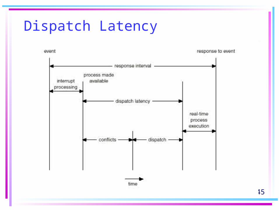
• Dispatch latency – time it takes for the dispatcher to stop one process and start running another…should be as fast as possible.
§ 6.1.4分派
10
Scheduling Criteria
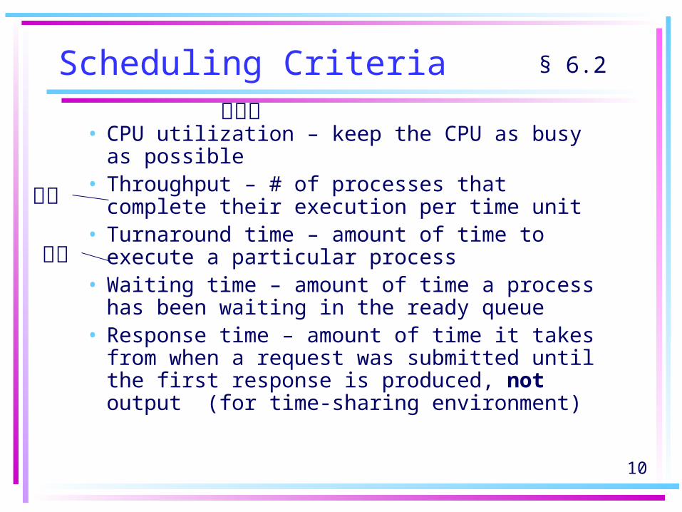
• CPU utilization – keep the CPU as busy as possible
• Throughput – # of processes that complete their execution per time unit
• Turnaround time – amount of time to execute a particular process
• Waiting time – amount of time a process has been waiting in the ready queue
• Response time – amount of time it takes from when a request was submitted until the first response is produced, not output (for time-sharing environment)
§ 6.2
產量
使用率
回復
11
Optimization Criteria
• Max CPU utilization• Max throughput• Min turnaround time • Min waiting time • Min response time
12
Scheduling Algorithms
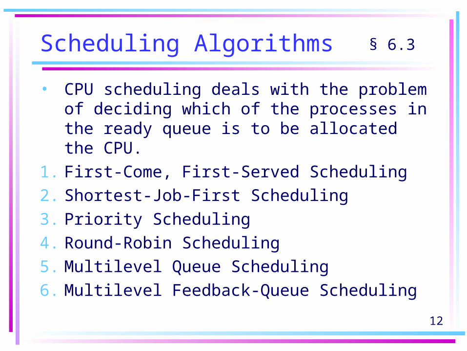
• CPU scheduling deals with the problem of deciding which of the processes in the ready queue is to be allocated the CPU.
1. First-Come, First-Served Scheduling2. Shortest-Job-First Scheduling3. Priority Scheduling4. Round-Robin Scheduling5. Multilevel Queue Scheduling6. Multilevel Feedback-Queue Scheduling
§ 6.3

13
First-Come, First-Served (FCFS) Scheduling
§ 6.3.1
....... CPU
Next in line toaccess the CPU
Process in controlof the CPU
Newprocessenterssystem
Queue of PCBs forprocesses waiting to run
Processfinishes
先到先做
14
First-Come, First-Served (FCFS) Scheduling
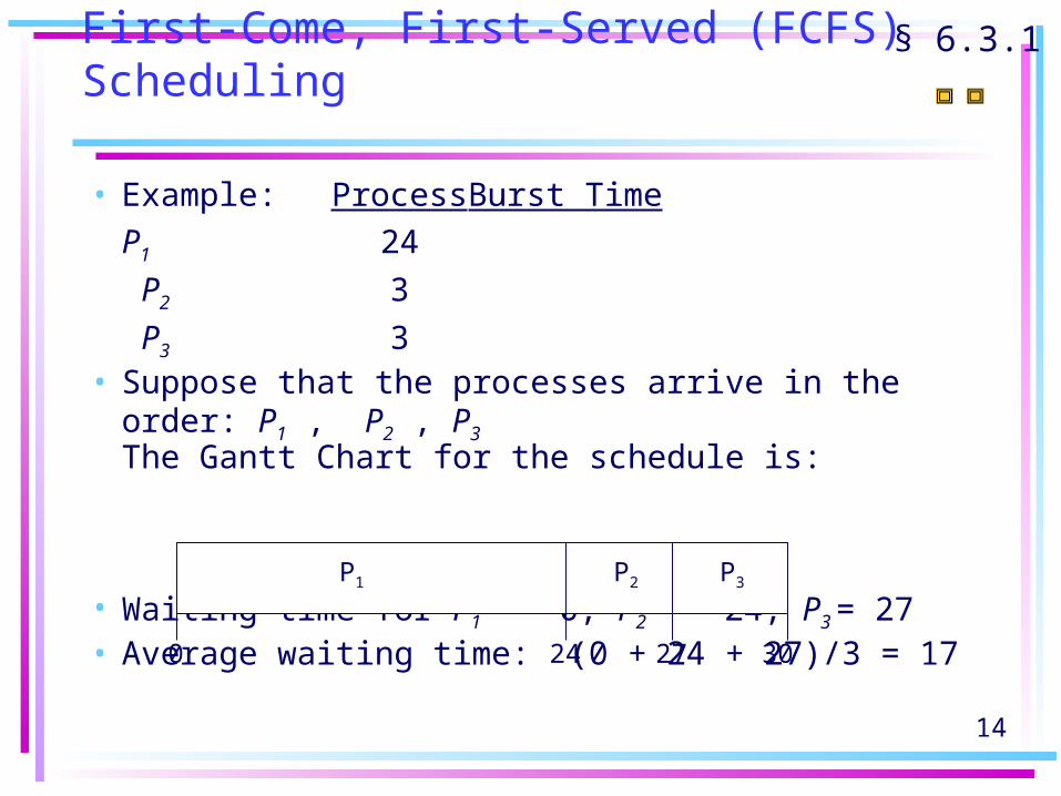
• Example: ProcessBurst TimeP1 24
P2 3
P3 3
• Suppose that the processes arrive in the order: P1 , P2 , P3
The Gantt Chart for the schedule is:
• Waiting time for P1 = 0; P2 = 24; P3 = 27• Average waiting time: (0 + 24 + 27)/3 = 17
P1 P2 P3
24 27 300
§ 6.3.1
15
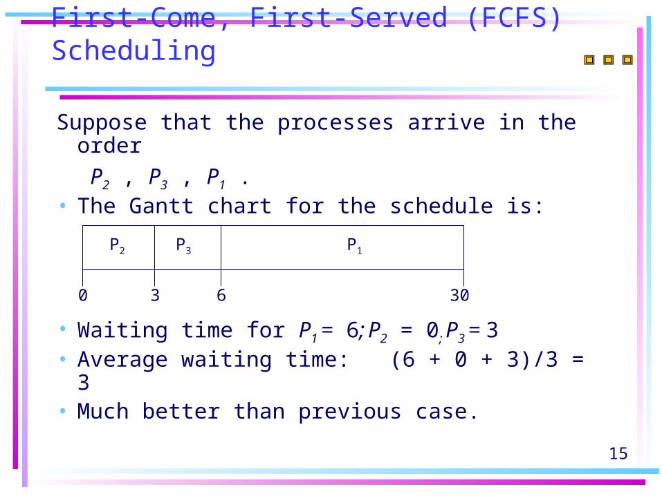
Suppose that the processes arrive in the order
P2 , P3 , P1 .• The Gantt chart for the schedule is:
• Waiting time for P1 = 6; P2 = 0; P3 = 3• Average waiting time: (6 + 0 + 3)/3 = 3• Much better than previous case.
P1P3P2
63 300
First-Come, First-Served (FCFS) Scheduling
16
• Convoy effect: many short processes waiting for one long process to get off the CPU……lower CPU and device utilization.
• FCFS scheduling algorithm is nonpreemptive.
First-Come, First-Served (FCFS) Scheduling
護航
17
Shortest-Job-First (SJF) Scheduling
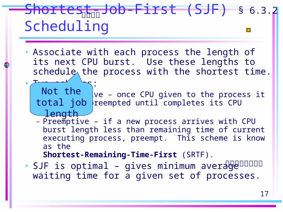
• Associate with each process the length of its next CPU burst. Use these lengths to schedule the process with the shortest time.
• Two schemes: – nonpreemptive – once CPU given to the process it
cannot be preempted until completes its CPU burst.– Preemptive – if a new process arrives with CPU
burst length less than remaining time of current executing process, preempt. This scheme is know as the Shortest-Remaining-Time-First (SRTF).
• SJF is optimal – gives minimum average waiting time for a given set of processes.
Not the total job length
§ 6.3.2最短先做
最短剩餘時間先做

18
Shortest-Job-First (SJF) Scheduling
Process Burst Time
P1 6
P2 8
P3 7
P4 3
• Average waiting time = (3 + 16 + 9 + 0)/4 = 7
• Compare to 10.25 milliseconds of FCFS
P1 P3 P2
93 160
P4
24

19
SJF Difficulty
• Knowing the length of the next CPU request is not easy.
• SJF used frequently in Long-term scheduling with the user specifies the length when he submits the job.
• SJF cannot be implemented at the level of short-term CPU scheduling…there is no way to know the length of the nest CPU burst.
• We can only approximate SJF by predicting the next CPU burst to be similar in length to the previous ones.
20
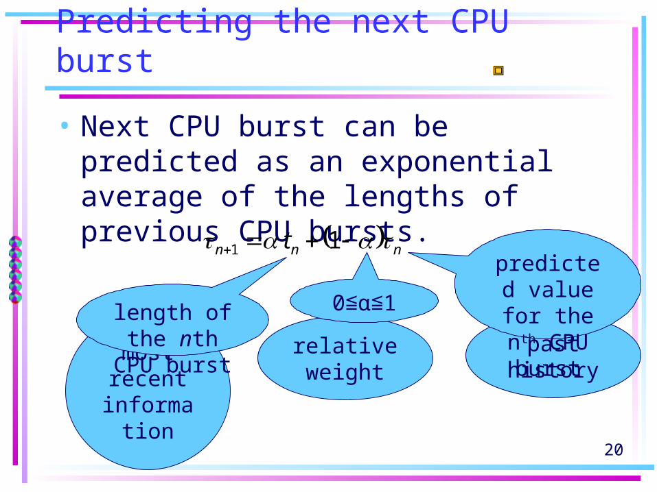
past historyrelative weightmost recent
information
Predicting the next CPU burst
• Next CPU burst can be predicted as an exponential average of the lengths of previous CPU bursts.
nnn t 1 1
length of the nth CPU
burst
predicted value for the
nth CPU burst
0≦α 1≦

21
=0 (Recent history does not count) n+1 = n
=1 (Only the actual last CPU burst counts)
– n+1 = t n
= ½ (recent history and past history are equally weighted)
Predicting the next CPU burst
22
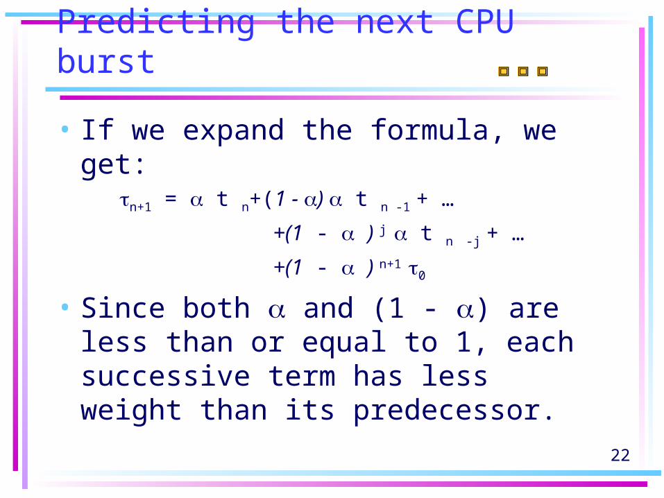
• If we expand the formula, we get:n+1 = t n+(1 - ) t n -1 + …
+(1 - ) j t n -j + …
+(1 - ) n+1 0
• Since both and (1 - ) are less than or equal to 1, each successive term has less weight than its predecessor.
Predicting the next CPU burst

23
Shortest-remaining-time-first scheduling
• When a new process arrives at the ready queue while a previous process is executing, the new process may preempt the currently executing process.
• Process Arrival Time Burst Time P1 0 8 P2 1 4 P3 2 9 P4 3 5
P1P2P1
105 260
P4 P3
1 17
average time:((10-1)+(1-1)+(17-2)+(5-3))/4= 6.5 millisecondsNonpreemptive SJF: 7.75
24
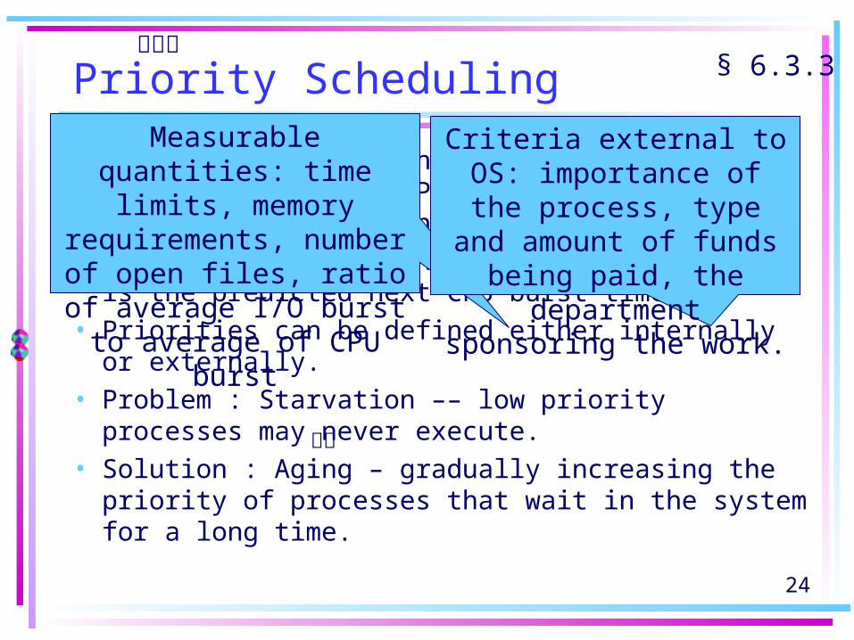
Priority Scheduling
• A priority number (integer) is associated with each process. CPU is allocated to the process with the highest priority
• SJF is a priority scheduling where priority is the predicted next CPU burst time.
• Priorities can be defined either internally or externally.
• Problem : Starvation –– low priority processes may never execute.
• Solution : Aging – gradually increasing the priority of processes that wait in the system for a long time.
§ 6.3.3
Measurable quantities: time limits, memory requirements, number of open files, ratio of average I/O burst to average
of CPU burst
Criteria external to OS: importance of the process, type and amount of funds being paid, the department
sponsoring the work.
老化
優先權

25
Round Robin (RR)
• Designed for time-sharing systems with preemption added to the FCFS scheduling.
• Each process gets a small unit of CPU time (time quantum), usually 10-100 milliseconds. After this time has elapsed, the process is preempted and added to the end of the ready queue.
• The average waiting time under RR is often long:
The average waiting time is 17/3=5.66 milliseconds
§ 6.3.4
P1 P2 P3 P1 P1 P1 P1 P1
0 4 7 10 14 18 22 26 30
Process Burst Time P1 24 P2 3 P3 3
依序循環
(環繞的知更鳥)
時間量
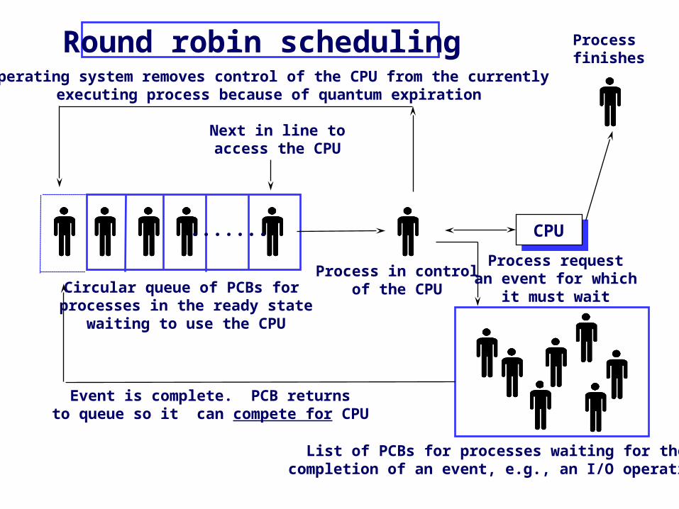
Round robin scheduling
....... CPU
Operating system removes control of the CPU from the currentlyexecuting process because of quantum expiration
Next in line toaccess the CPU
Circular queue of PCBs for processes in the ready state
waiting to use the CPU
Processfinishes
Process requestan event for which
it must wait
Process in controlof the CPU
Event is complete. PCB returnsto queue so it can compete for CPU
List of PCBs for processes waiting for thecompletion of an event, e.g., an I/O operation

27
Round Robin (RR)
• If there are n processes in the ready queue and the time quantum is q, then each process gets 1/n of the CPU time in chunks of at most q time units at once. No process waits more than (n -1)q time units.
• Performance– q large FIFO– q small Called processor sharing, appears
as n processes running at 1/n the speed of the real processor. (q must be large with respect to context switch, otherwise overhead is too high.)
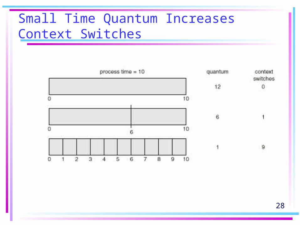
28
Small Time Quantum Increases Context Switches
29
Turnaround time v.s. time quantum
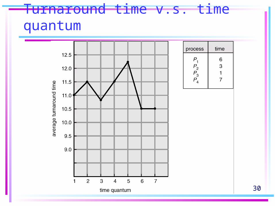
• The average turnaround time of a set of processes does not necessarily improve as the time-quantum size increases.
• In general, the average turnaround time can be improved if most processes finish their next CPU burst in a single time quantum.
30
Turnaround time v.s. time quantum

31
Multilevel Queue Scheduling
• Each queue has its own scheduling algorithm • The processes are assigned to one queue based
on some property of the process, such as memory size, process priority, or process type.
• Scheduling must be done between the queues.– Fixed priority scheduling; i.e., serve all from foreground
then from background. Possibility of starvation.– Time slice – each queue gets a certain amount of CPU
time which it can schedule amongst its processes; i.e.,80% to foreground in RR, 20% to background in FCFS
§ 6.3.5
foreground (interactive)background (batch)
– RoundRobin– FCFS
• Ready queue is partitioned into separate queues:
多層佇列
32
Multilevel Queue Scheduling
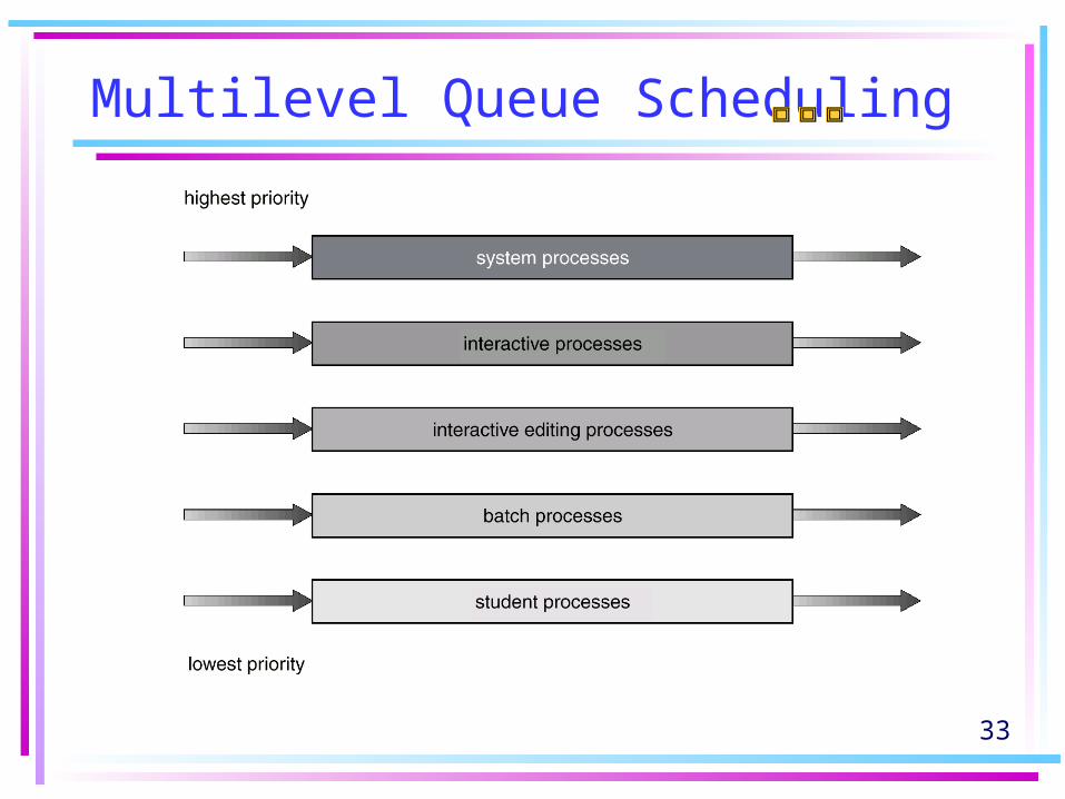
• There must be scheduling between the queues. Example: Fig. 6.6 (Each queue has absolute priority over lower-priority queues.)
1. Fixed-priority preemptive scheduling:– No process in the lower queue could run unless
the higher queues were empty.– If higher level process entered the ready queue
while a lower level process was running, the lower level process would be preempted.
2. Time slice between the queue: Each queue gets a certain portion of the CPU time.
33
Multilevel Queue Scheduling
34
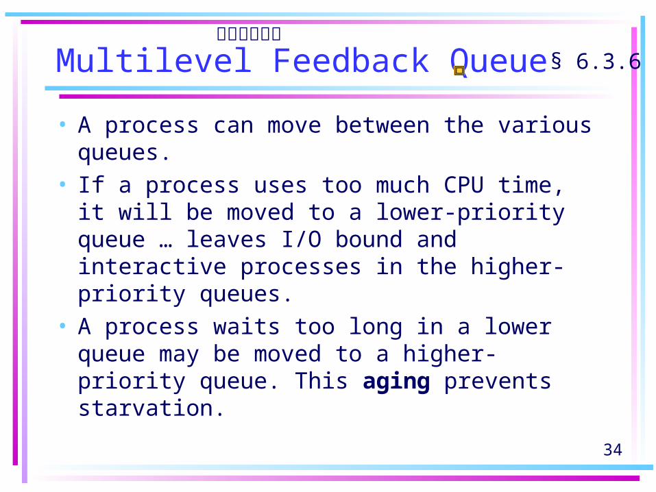
Multilevel Feedback Queue
• A process can move between the various queues.
• If a process uses too much CPU time, it will be moved to a lower-priority queue … leaves I/O bound and interactive processes in the higher-priority queues.
• A process waits too long in a lower queue may be moved to a higher-priority queue. This aging prevents starvation.
§ 6.3.6多層回饋佇列

35
Multilevel Feedback Queue
• Example:Three queues: – Q0 – time quantum 8 milliseconds– Q1 – time quantum 16 milliseconds– Q2 – FCFS
• Scheduling– A new job enters queue Q0 which is served FCFS.
When it gains CPU, job receives 8 milliseconds. If it does not finish in 8 milliseconds, job is moved to queue Q1.
– At Q1 job is again served FCFS and receives 16 additional milliseconds. If it still does not complete, it is preempted and moved to queue Q2.

36
Multilevel Feedback Queue
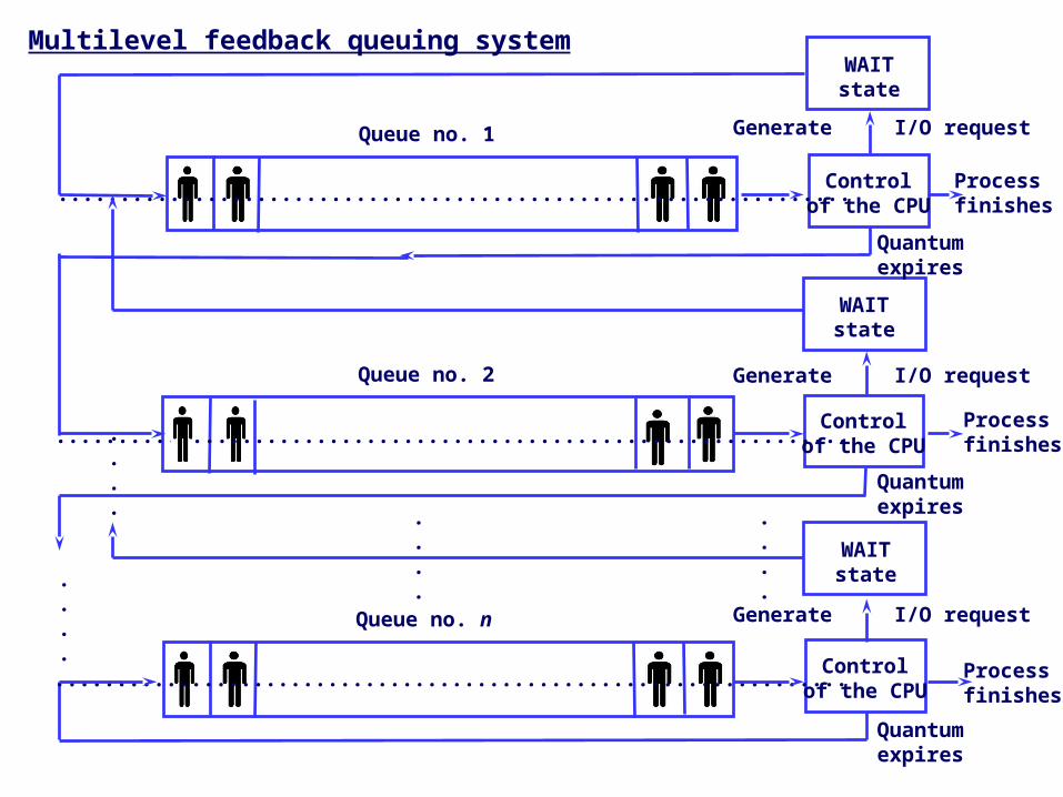
WAITstate
Controlof the CPU
Queue no. 1
................................................................
WAITstate
Controlof the CPU
Queue no. 2
................................................................
WAITstate
Controlof the CPU
Queue no. n
................................................................
.
.
.
.
.
.
.
.
.
.
.
.
.
.
.
.
Generate I/O request
Generate I/O request
Generate I/O request
Processfinishes
Processfinishes
Processfinishes
Quantumexpires
Quantumexpires
Quantumexpires
Multilevel feedback queuing system
38
Multilevel Feedback Queue
• Multilevel-feedback-queue scheduler defined by the following parameters:– number of queues– scheduling algorithms for each queue– method used to determine when to upgrade a process– method used to determine when to demote a process– method used to determine which queue a process will
enter when that process needs service
• Although multilevel feedback queue is the most general scheme, it is also the most complex for the necessary of selecting values for all the parameters to define the best scheduler.
39
Multiple-Processor Scheduling
• CPU scheduling more complex when multiple CPUs are available.
• We concentrate on systems in which the processors are identical – Homogeneous.
• if several identical processors are available, then Load sharing can occur…provide a separate queue for each processor.
• To prevent load unbalance, use a common ready queue. All processes go into one queue and are scheduled onto any available processor.
Two possible schemes
§ 6.4
40
Multiple-Processor Scheduling
• Symmetric Multiprocessing (SMP) – each processor makes its own scheduling decisions. Each processor examines the common ready queue and selects a process to execute.
• Asymmetric multiprocessing – having all scheduling decisions, I/O processing, and other system activities handled by one single processor – the master server. The other processors execute only user code. It is simpler because only one processor accesses the system data structures, alleviating the need for data sharing.

41
Real-Time Scheduling
• Hard real-time systems – required to complete a critical task within a
guaranteed amount of time.– Need resource reservation. The scheduler know
exactly how long it takes to perform each type of OS function.
– Lack the full functionality of modern computers and OS.
• Soft real-time computing – requires that critical processes receive priority over
less fortunate ones.– Although may cause unfair allocation of resources
and longer delays for some processes, it is at least possible to achieve
§ 6.5

42
Implementing soft real-time function
1. The system must have priority scheduling, and real-time processes must have the highest priority.
2. The dispatch latency must be small. relatively simple
to holdnot easy to ensure. The latency can be
long since some system calls are
complex and some I/O devices are slow.

43
Real-Time Scheduling
• To keep dispatch latency low, we need to allow system calls to be preemptible. Ways to achieve this goal:
1. insert preemption points in long-duration system calls.
2. make the entire kernel preemptible. To ensure correct operation, all kernel data structures must be protected through the use of various synchronization mechanisms.
check to see whether a high-priority process
needs to be run. If it does, a context switch takes place.

44
Priority Inversion
• Higher-priority process needs to wait when it needs to read or modify kernel data that are currently being accessed by another lower-priority process.
• If there is a chain of lower-priority processes, they inherit the high priority until they are done with the resources. ––– priority-inheritance protocol
45
Dispatch Latency

46
Algorithm Evaluation
• When selecting a CPU scheduling algorithm for a particular system, different evaluation methods may be used:– Deterministic Modeling– Queueing Models– Simulations– Implementation
§ 6.6

47
Deterministic Modeling
• Analytic evaluation uses the given algorithm and the system workload to produce a formula or number that evaluates the performance of the algorithm for that workload.
• One type of analytic evaluation is deterministic modeling. It takes a particular predetermined workload and defines the performance of each algorithm for that workload.
• Example:
Process Burst Time P1 10 P2 29 P3 3 P4 7 P5 12
Consider the FCFS, SJF, and RR (quantum= 10 milliseconds). Which algorithm wouldgive the minimumaverage waiting time?
§ 6.8.1

48
Deterministic Modeling
P1 P2 P3 P4P5
P3 P4 P1 P5 P2
P1 P2 P3 P4 P5 P2 P5 P2
0 10 39 42 49 61
0 3 10 20 32 61
0 10 20 23 30 40 50 52 61
FCFS: Average waiting time is (0+10+39+42+49)/5=28 ms
SJF: Average waiting time is (10+32+0+3+20)/5=13 ms
RR: Average waiting time is (0+32+20+23+40)/5 = 23 ms

49
Deterministic Modeling
• Deterministic modeling is simple and fast. It gives exact numbers, allowing the algorithms to be compared.
• However, it requires exact number for input, and its answers apply to only those cases.
• The main uses are in describing scheduling algorithms and providing examples…too specific, and requires too much exact knowledge, to be useful
• Used when the same program may be ran over and over again and can measure the program’s processing requirements exactly.

50
Queueing Models
• Processes vary, no static set of processes to use for deterministic modeling.
• What can be determined is the distribution of CPU and I/O bursts.
• These distributions may be measured and then approximated. The result is a mathematical formula describing the probability of a particular CPU burst.
• Arrival-time distribution given the distribution of times when processes arrive in the system.
• From these two distribution, it is possible to compute the average throughput, utilization, waiting time, and so on for most algorithm.
§ 6.8.2
51
Queueing Models
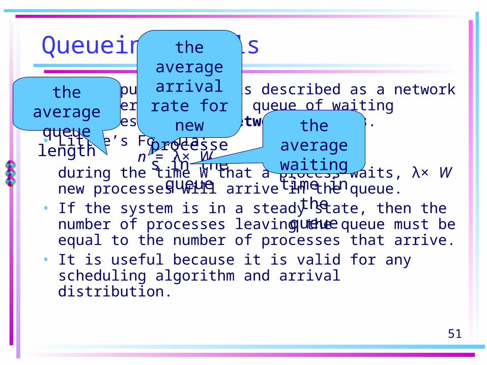
• The computer system is described as a network of servers each has a queue of waiting processes…queueing-network analysis.
• Little’s Formula: n = λ× Wduring the time W that a process waits, λ× W new processes will arrive in the queue.
• If the system is in a steady state, then the number of processes leaving the queue must be equal to the number of processes that arrive.
• It is useful because it is valid for any scheduling algorithm and arrival distribution.
the average queue length
the average arrival rate
for new processes in
the queue the average waiting time in the queue

52
Queueing Models
• Example: seven processes arrive every second (on average), normally 14 processes in the queue, the average waiting time per process is 2 seconds.
• Limitations:– The classes of algorithms and distributions
that can be handled are limited.– The mathematics of complicated algorithms
or distributions can be difficult to work with.– Arrival and service distributions are often
defined in unrealistic, but mathematically tractable, ways.
53
Simulations
• Programming a model of the computer system with data structures represent the major components of the system.
• The simulator modifies the system state to reflect the activities of the devices, the processes, and the scheduler.
• As the simulation executes, statistics that indicate algorithm performance are gathered and printed.
• More accurate evaluation than queueing models.
§ 6.8.3
54
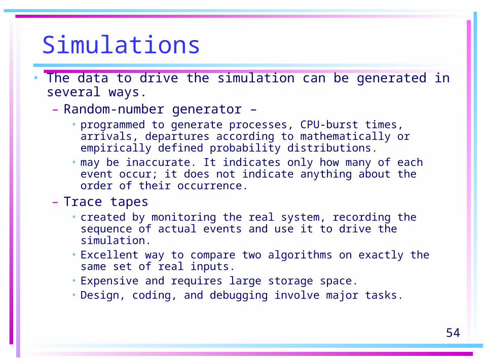
Simulations• The data to drive the simulation can be generated in
several ways.– Random-number generator –
• programmed to generate processes, CPU-burst times, arrivals, departures according to mathematically or empirically defined probability distributions.
• may be inaccurate. It indicates only how many of each event occur; it does not indicate anything about the order of their occurrence.
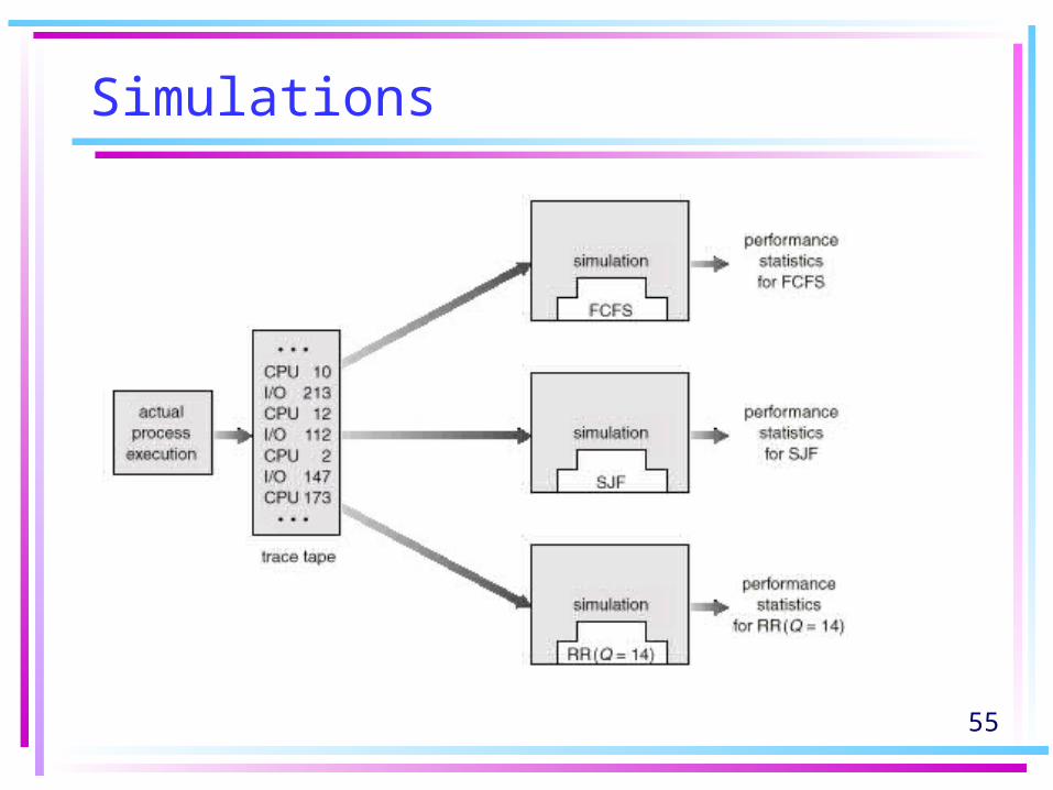
– Trace tapes• created by monitoring the real system, recording the
sequence of actual events and use it to drive the simulation.• Excellent way to compare two algorithms on exactly the
same set of real inputs.• Expensive and requires large storage space.• Design, coding, and debugging involve major tasks.
55
Simulations
56
Implementation
• The only completely accurate way to evaluate a scheduling algorithm is to code it up, to put it in the OS, and to see how it works.
• Major difficulty: – high cost– the environment in which the
algorithm is used will change.

57
Process Scheduling Models
• Process Local Scheduling – How the threads library decides which thread to run on an available LWP. (more software-library than OS concern)
• System Global Scheduling – How the kernel decides which kernel thread to run next. (This text cover global scheduling only)
§ 6.7
58
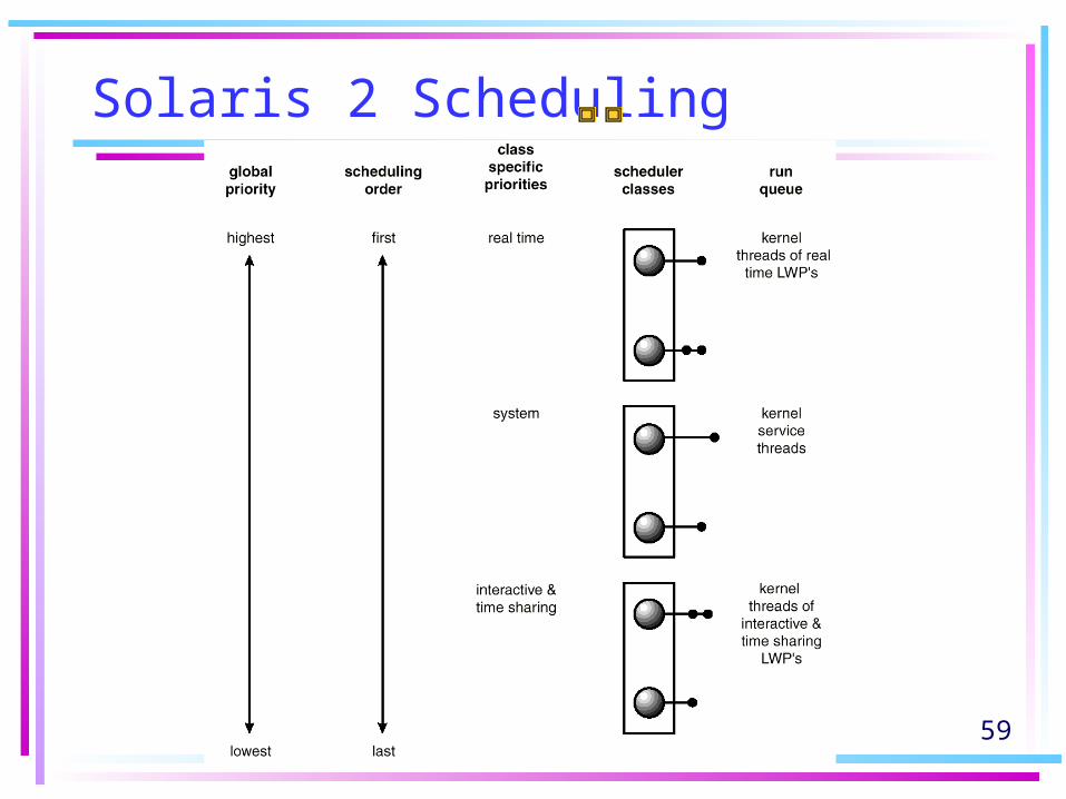
Solaris 2 Scheduling
• Priority-based process scheduling• Four classes of scheduling: real
time, system, time sharing, interactive.
• Within each class there are different priorities and different scheduling algorithms.
• Default scheduling class for a process is time sharing.
§ 6.7.1
59
Solaris 2 Scheduling

60
Solaris 2 Scheduling
1. Time sharing:– dynamically alters priorities and
assigns time slices of different lengths using a multilevel feedback queue.
– Interactive processes typically have a higher priority; CPU-bound processes a lower priority.
– gives good response time for interactive processes and good throughput for CPU-bound processes
61
Solaris 2 Scheduling
2. Interactive class:– same scheduling policy as time-sharing
but gives windowing applications a higher priority for better performance.
3. System class:– uses it to run kernel processes, such as
the scheduler and paging daemon.
4. real-time class:– gives the highest priority to run among all
classes. Allows a real-time process to have a guaranteed response from the system within a bounded period of time.
– A real-time process will run before a process in any other class.
62
Windows 2000
• Windows 2000 schedules threads using a priority-based, preemptive scheduling algorithm.
• A thread selected to run by the Dispatcher will run until it is preempted by– a higher-priority thread– terminates– time quantum ends– calls a blocking system call (e.g. I/O)
§ 6.7.2
63
Windows 2000 Real-time thread
• Preemption allow real-time threads to access the CPU.
• However, Windows 2000 is not hard-real time OS, because it does not guarantee that a real-time thread will start to execute within any particular time limit.
64
The dispatcher
• The Windows 2000 dispatcher uses a 32-level scheme to determine the order of thread execution.
• Priorities are divided into two classes:– the variable class contains threads having
priorities from 1 to 15– the real-time class contains threads with
priorities ranging from 16 to 31(priority 0 for memory management)

65
The dispatcher
• A queue for each scheduling priority, traverses the set of queues from highest to lowest until it finds a thread that is ready to run.
• If no thread is found, the dispatcher will execute a special thread called the idle thread.

66
Priorities
• The numeric priorities of the Windows 2000 threads are identified by the Win32 API.
• Priority classes:– REALTIME_PRIORITY_CLASS– HIGH_PRIORITY_CLASS– ABOVE_NORMAL_PRIORITY_CLASS– NORMAL_PRIORITY_CLASS– BELOW_NORMAL_PRIORITY_CLASS– IDLE_PRIORITY_CLASS
67
Priorities
• All priority classes except the REALTIME_
PRIORITY_CLASS are variable class priority.• Within each of these priority classes is
a relative priority which has value:– TIME_CRITICAL– HIGHEST– ABOVE_NORMAL– NORMAL– BELOW_NORMAL– LOWEST– IDLE

68
Priorities
• The priority of each thread is based upon the priority class it belongs to and the relative priority within the class
realtime
high abovenormal
normal belownormal
idlepriority
time-critical 31 15 15 15 15 15
highest 26 15 12 10 8 6
above normal
25 14 11 9 7 5
normal 24 13 10 8 6 4
below normal
23 12 9 7 5 3
lowest 22 11 8 6 4 2
idle 16 1 1 1 1 1
base priority
69
Priorities
• Processes are typically members of the NORMAL_PRIORITY_CLASS.
• The initial priority of a thread is typically the basic priority of the process the thread is belongs to.
• When a thread’s time quantum runs out, that thread is interrupted and its priority is lowered.
70
Priorities
• When a variable-priority thread is released from a wait operation, the dispatcher boosts the priority.
• The amount of the boost depends on what the thread was waiting for. Ex:– thread waiting for keyboard I/O would
get a large priority increase– thread waiting for disk operation
would get a moderate one.
Give good response times to interactive threads that are using the mouse and windows, and enables I/O-bound threads to keep the I/O device busy.
while permitting compute-bound threads to use spare CPU cycles in the background.
This strategy is used by several time-sharing OS, including UNIX.

71
Foreground vs. Background
• Windows 2000 distinguishes processes in the NORMAL_PRIORITY_CLASS between foreground process and background processes.
• When a process moves into the foreground, Windows 2000 increases the scheduling quantum by some factor – typically 3 (a three times longer time to run).
72
Linux
• Two separate process-scheduling algorithms:1. for conventional, time-sharing processes, a
prioritized, credit-based algorithm doing fair preemptive scheduling among multiple processes.
2. for real-time tasks taking priorities as more important factor than fairness.
Part of every process’ identity is a scheduling class, that defines which of these algorithms to apply to the process.
§ 6.7.3
73
Scheduling time-sharing processes
• Each process possesses a certain number of scheduling credits.
• When a new task must be chosen to run, the process with the most credits is selected.
• Every time a timer interrupt occurs, the currently running process loses one credit; when its credits reaches zero, it is suspended and another process is chosen.
74
Scheduling time-sharing processes
• If no runnable processes have any credits, then Linux performs a recrediting operation, adding credits to every process in the system, according to the following rule:credits = (credits / 2) + priority
retaining some history of the process’ recent behavior
Processes that are running all the time tend to exhaust their credits rapidly, but processes that
spend much of their time suspended can accumulate credits over multiple recreditings and consequently end up with a higher credit
count after a recredit.
75
Scheduling time-sharing processes
• The crediting system automatically gives high priority to interactive or I/O bound processes, for which a rapid response time is important.
• Background batch jobs get low priority automatically while receiving fewer credits than interactive jobs.
76
Scheduling real-time processes
• Linux implements the two real-time scheduling classes required by POSIX.1b: FCFS and Round-robin.
• Linux’s real-time scheduling is soft – rather than hard – real time.The scheduler offers strict guarantees about the
relative priorities of real-time processes, but the kernel does not offer any guarantees about how quickly a real-time process will be scheduled.
Recommended