

KM3NeT: Technical Design Report
6
G. Bourlis, P. E. Christopoulou, I. Gialas, N. Gizani, A. Leisos, C. Papageorgiou, A. Tsirigotis, S. Tzamarias
Hellenic Open University, Patras, Greece
E. Barbarito, A. Ceres, M. Circella, M. Mongelli, M. Romita
INFN Sezione Bari and University of Bari, Italy
M. Bazzotti, S. Biagi, G. Carminati, S. Cecchini, T. Chiarusi, G. Giacomelli, A. Margiotta, M. Spurio
INFN Sezione Bologna and University of Bologna, Italy
S. Aiello, L. Caponetto, A. Grimaldi, E. Leonora, D. Lo Presti, N. Randazzo, S Reito, G.V. Russo, D. Sciliberto, V. Sipala, S. Urso
INFN Sezione di Catania and University of Catania, Italy
M. Anghinolfi, A. Bersani, M.Battaglieri, M. Brunoldi, R. Cereseto, R.DeVita, H. Costantini, K. Fratini, S. Minutoli, P. Musico,
M. Osipenko, D. Piombo, G. Ricco, M. Ripani, M. Taiuti, D. Torazza
INFN Sezione Genova and University of Genova, Italy
I. Amore, G. Cacopardo, R. Cocimano, R. Coniglione, M. Costa, A. D’Amico, C. Distefano, V. Giordano, M. Imbesi, D. Lattuada,
E. Migneco, M. Musumeci, A. Orlando, R. Papaleo, V. Pappalardo, P. Piattelli, G. Raia, G. Riccobene, A. Rovelli, P. Sapienza, M. Sedita,
A. Trovato, S. Viola
INFN Laboratori Nazionali del Sud, Catania, Italy
R. Habel, A. Martini, L. Trasatti
INFN Laboratori Nazionali di Frascati, Italy
G. Barbarino, G. De Rosa , S. Russo
INFN Sezione Napoli and University of Napoli, Italy
E. Castorina, V. Flaminio, R. Garaguso, D. Grasso, A. Marinelli, M. Morganti, C. Sollima
INFN Sezione Pisa and University of Pisa, Italy
F. Ameli, M. Bonori, A. Capone, G. De Bonis, F. Lucarelli, R. Masullo, F. Simeone, M. Vecchi
INFN Sezione Roma and University of Roma 1, Italy
B. Bigourdan, P. Bouquet, D. Choqueuse, G. Damy, J. Drogou, Z. Guédé, J. Marvaldi, J. Rolin, P. Valdy
IFREMER, France
G. Etiope, P. Favali, C. La Fratta, G. Marinaro
Istituto Nazionale di Vulcanologia, Italy
G, Guillard T. Pradier
University of Strasbourg and Institut Pluridisciplinaire Hubert Curien/IN2P3/CNRS, Strasbourg, France
D. Felea, O. Maris, G. Pavalas, V. Popa, A. Radu, M. Rujoiu, D. Tonoiu
Institute of Space Sciences, Machurele Bucharest, Romania

7
KM3NeT: Technical Design Report
N. Bellou, F. Colijn, P. Koske, T. Staller
University of Kiel, Germany
N. Kalantar‐Nayestanaki, O. Kavatsyuk, H. Löhner
KVI and University of Groningen, the Netherlands
S. Bradbury, J. Rose, R.J. White
University of Leeds, United Kingdom
F. Jouvenot, C. Touramanis
University of Liverpool, United Kingdom
D. Lenis, E.C. Marcoulaki, C. Markou, I.A. Papazoglou, P.A. Rapidis, I. Siotis, E. Tzamariudaki
National Center of Scientific Research “Demokritos”, Athens, Greece
A. Assis Jesus, E. Berbee, A. Berkien, R. de Boer, H. Boer Rookhuizen, M. Bouwhuis, C. Chen, P. Decowski, D. Gajanana,
A. Heijboer, E. Heine, M. van der Hoek, J. Hogenbirk, P. Jansweijer, M. de Jong, H. Kok, A. Korporaal, S. Mos, G. Mul, D. Palioselitis,
H. Peek, E. Presani, C. Reed, D. Samtleben, J.‐W. Schmelling, J.Steijger, P. Timmer, P. Werneke, G. Wijnker
NIKHEF, Amsterdam, the Netherlands
R. Bakker, R. Groenewegen, H. van Haren, T. Hillebrand, J. van Heerwaarden, M. Laan, M. Smit
Koninklijk Nederlands Instituut voor Onderzoek der Zee (NIOZ), Texel, the Netherlands
T. Athanasopoulos, A. Ball, A. Belias, A. Fotiou, Y. Kiskiras, A. Kostoglou, S. Koutsoukos,
M. Maniatis, E. Markopoulos, A. Psallidas, L.K. Resvanis, G. Stavropoulos, V. Tsagli, G. Vermisoglou, V. Zhukov
NOA / NESTOR, Pylos, Greece
J. Perkin, L. Thompson
University of Sheffield, United Kingdom
F. Gasparoni, F.Bruni
Tecnomare, Venice, Italy
E. Kendziorra, A. Santangelo
University of Tübingen, Germany
P. Kooijman
University of Utrecht and University of Amsterdam, the Netherlands
C. Bigongiari, U. Emanuele, H. Yepes, J. Zúñiga
University of Valencia, Spain
J. Alba, M. Ardid, M. Bou‐Cabo, F. Camarena, V. Espinosa, G. Larosa, J. Martínez‐Mora, J. Ramis, J. Redondo, V. Sánchez‐Morcillo
Universidad Politécnica Valencia / IGIC, Spain


KM3NeT: Technical Design Report
10
3.5 Calibration and Positioning
3.5.1 Time calibration
3.5.2 Positioning
3.5.3 Charge calibration
3.5.4 Water and Environmental monitoring
3.6 Assembly of optical modules
3.6.1 Detection unit integration
3.7 Marine Operations
3.7.1 Deployment and connection
3.7.2 Vessels
4 Earth and sea sciences infrastructure
4.1 General description
4.2 Junction box
4.3 Connectivity
4.3.1 Main Uplink Cable
4.3.2 Uplink Cable connection
4.3.3 Power Converter and interfaces
4.3.4 Downlink Cables
4.3.5 Connector Manifold plate
4.3.6 Docking Unit with foundations
4.4 Deployment and Maintenance
4.5 Marine Operations
4.6 Additional Features
5 Site Characterisation
5.1 Locations
5.1.2 Weather and Sea Conditions
5.1.3 Geology
5.2 Environmental Site Characteristics
5.2.1 Temperature
5.2.2 Salinity
5.2.3 Deep‐sea Currents
5.2.4 Sedimentation and Biofouling
5.2.5 Radioactivity
5.2.6 Bioluminescent Organisms
84
84
86
88
88
89
97
102
103
104
107
107
108
112
112
113
113
113
113
114
114
114
114
117
117
119
120
120
121
121
121
123
126
127
...................................................................................................
...................................................................................................
...................................................................................................
...................................................................................................
...................................................................................................
...................................................................................................
...................................................................................................
...................................................................................................
...................................................................................................
...................................................................................................
...........................................................................
...................................................................................................
...................................................................................................
...................................................................................................
...................................................................................................
...................................................................................................
...................................................................................................
...................................................................................................
...................................................................................................
...................................................................................................
...................................................................................................
...................................................................................................
..................................................................................................
...........................................................................
...................................................................................................
...................................................................................................
...................................................................................................
...................................................................................................
...................................................................................................
...................................................................................................
...................................................................................................
...................................................................................................
...................................................................................................
...................................................................................................

11
KM3NeT: Technical Design Report
5.3 Optical Properties of the Deep‐Sea Environment
5.3.1 Light Transmission Parameters
5.3.2 Light Transmission Measurements
5.3.3 Background Light Measurements
6 Telescope Performance
6.1 Analysis Techniques
6.1.1 Background Suppression
6.1.2 Online Data Filter
6.1.3 Muon Reconstruction
6.1.4 Sensitivity Calculation
6.2 Simulation
6.2.1 ANTARES Software
6.2.2 SeaTray
6.2.3 Alternative Simulations
6.2.4 Sea water properties used in simulations
6.3 Sensitivity Studies
6.3.1 Detector Optimization and Performance
6.3.2 Neutrino Point Sources
6.3.3 Transient Sources
6.3.4 Diffuse Fluxes
6.3.5 Dark Matter
7 Ecological Impact and Decommissioning
7.1 Construction and Commissioning
7.2 Operations and Maintenance.
7.3 Decommissioning
7.4 Legacy Post Decommissioning
8 Quality Assurance and Reliability
8.1 Methodology
8.2 Quality Management System
8.2.1 Quality Assurance Manual
8.3 Risk Assessment
8.4 Dependability analysis
8.4.1 Results of the dependability analysis
8.5 Failure mode and effect analyses
128
128
129
131
135
135
135
136
136
137
138
138
138
139
140
140
141
143
147
149
152
155
155
155
156
156
159
159
161
161
165
165
168
169
...................................................................................................
...................................................................................................
...................................................................................................
...................................................................................................
...........................................................................
...................................................................................................
...................................................................................................
...................................................................................................
...................................................................................................
...................................................................................................
...................................................................................................
...................................................................................................
...................................................................................................
...................................................................................................
...................................................................................................
...................................................................................................
...................................................................................................
...................................................................................................
...................................................................................................
...................................................................................................
...................................................................................................
...........................................................................
...................................................................................................
...................................................................................................
...................................................................................................
...................................................................................................
...................................................................................................
...................................................................................................
...................................................................................................

KM3NeT: Technical Design Report
12
8.6 Quality Control
8.6.1 General rules for the quality
control definition
9 Cost and Feasibility of Construction
9.1 Capital Investment
9.2 Running costs
9.3 Maintenance
10 Implementation
10.1 Decision Path and Development Plan
10.1.1 Decisions and Resources
10.1.2 Consortium Organisation
10.1.3 Time lines
10 2 Future Project Structure
10 2.1 Governance
10 2.2 Project Management
11 Conclusions
Glossary
Bibliography
170
171
175
175
176
177
181
181
181
182
182
182
183
183
185
187
191
...................................................................................................
...................................................................................................
...........................................................................
...................................................................................................
...................................................................................................
...................................................................................................
...........................................................................
...................................................................................................
.................................................................................................
.................................................................................................
.................................................................................................
.................................................................................................
.................................................................................................
.................................................................................................
...........................................................................
...........................................................................
...........................................................................

13
KM3NeT: Technical Design Report
KM3NeT is a deep‐sea multidisciplinary observatory in the Mediterranean Sea that will provide innovative science
opportunities spanning Astroparticle Physics and Earth and Sea Science. This is possible through the synergy created by the
use of a common infrastructure allowing for long term continuous operation of a neutrino telescope and marine
instrumentation. The present KM3NeT Design Study concludes with this Technical Design Report which develops the ideas
put forward in the Conceptual Design Report published in April 2008 [1].
Neutrino astronomy opens a unique new window for the observation of the Universe. At the present time, the most sensitive
neutrino telescope in the world is the IceCube detector at the South Pole which in its final configuration will instrument a
cubic kilometre of polar ice. Building on the experience gained with the ANTARES neutrino telescope and other projects in the
Mediterranean Sea, the construction of the KM3NeT infrastructure is projected with a sensitivity exceeding that of IceCube by
a substantial factor. KM3NeT will be an essential node in the global network of multimessenger instruments in astronomy.
The principal goal of KM3NeT is the observation of cosmic point‐like sources of neutrinos, in particular in a region of the sky
complementary to the field of view of IceCube. This science objective has been the driving consideration in the optimization
of the detector design. The resulting sensitivity is compared to that of IceCube in the figure below, showing that KM3NeT ex-
tends substantially the visible region of the sky and even improves the discovery potential in the same field of view. This gain
is due to the far larger instrumented volume possible with the project budget, together with the significantly better angular
resolution achievable in water compared to ice.
The hostile environment of the deep sea together with the envisaged operation over at least 10 years, impose severe con-
straints on the telescope design. The design presented conforms to all these requirements within a budget of 250 M€ and
surpasses the original objective of the Design Study substantially. A strategy to pursue technical alternatives for critical
aspects, in particular the mechanical structure of the detection units, has been adopted. All solutions have a similar cost for
equal performance but remain to be fully evaluated for viability. The feasibility of construction has been addressed together
with environmental aspects and decommissioning issues.
Unprecedented prospects for real‐time data collection from the deep sea are provided with the observatory instruments.
Science fields such as climatology, geosciences, marine biology and oceanography will profit enormously from these data.
Representatives from these communities are involved in the design stage to ensure compatibility with their needs.
Different potential sites have been identified and investigated in detail. The site decision will be taken in the framework of the
ongoing KM3NeT Preparatory Phase project.
Final technical and site decisions will be made at the end of 2011 and a technical proposal will be presented in early 2012.
Final prototyping and construction could begin in 2013. Data taking will already start during the construction period of about
five years with first science data anticipated in 2014.
Executive summary


This document describes the technical design of a future deep‐sea research infrastructure in the Mediterranean Sea hosting
a multi‐cubic‐kilometre neutrino telescope and scientific nodes for longterm, continuous measurements in earth and marine
scientific research.
The science case for the neutrino telescope is overwhelming: Neutrinos are unique messengers from the most violent, high-
est‐energy processes in our Galaxy and far beyond. Their measurement will allow for new insights into the mechanisms and
processes that govern the non‐thermal Universe and will complement high‐energy gamma ray astronomy and cosmic ray
studies. The multi‐messenger picture emerging from these modalities of observation is one of the most exciting future
prospects of astronomy and astrophysics.
Neutrino astronomy is experimentally highly demanding, in particular since it requires vast volumes of target material, most
easily implemented in naturally abundant, transparent media, such as water or ice. It therefore took more than 20 years for the
field to mature from first‐generation pilot projects to large‐scale neutrino observatories. Currently, the world’s largest neutrino
telescope, IceCube, is under construction at the South Pole and will encompass one cubic kilometre of glacial ice in its final
configuration. KM3NeT will be significantly larger, exceeding IceCube in its sensitivity and complementing its field of view.
In particular, KM3NeT will have the Galactic Centre and a large part of the Galactic plane in its field of view most of the time.
It thus offers a prime observation opportunity for various types of Galactic candidate sources of neutrinos.
The construction of a deep‐sea neutrino telescope is technically highly challenging: the components must withstand the
enormous pressure and chemically aggressive sea water whilst being reliable enough to minimize complex maintenance
operations. The deployment operations must be safe, robust and precise. The design described here builds on the extensive
experience gained in the Mediterranean pilot projects ANTARES, NEMO and NESTOR, as well as on deep‐sea know‐how from
other fields of science and industry. A major step forward was the ultimate proof of feasibility for a deep‐sea neutrino
telescope provided by the successful installation and operation of the ANTARES experiment.
In the past four years, an in‐depth design study1 for KM3NeT has been performed, where existing technologies and design
solutions have been developed further and new approaches evaluated, tested and verified. Optimising the design for cost
effectiveness, feasibility of construction and reliability of operation narrowed down the design options to a scenario with a
limited number of alternative solutions. Final decisions will require further studies including prototyping efforts and
field tests.
The deep‐sea infrastructure of the neutrino telescope also offers unique possibilities for a wide spectrum of other research
activities, such as in environmental sciences, geology and geophysics, marine biology and oceanography. Furthermore, it could
be used to provide information for future hazard warning systems. The KM3NeT installation will be an important node in a
global network of deep‐sea observatories, operated by the projects ESONET, EMSO, GMES in Europe, Neptune Canada,
DONET Japan and the US OOI.
1 Funded through EU FP6, contract number 011937.
15
1. Introduction
KM3NeT: Technical Design Report

KM3NeT: Technical Design Report
16
In recognition of its unique, multidisciplinary scientific potential and its advanced technical status, KM3NeT was selected as
one of 35 European priority research infrastructures by the ESFRI2 panel in 2006; this status was confirmed in the 2008 review
process. As a consequence, KM3NeT is receiving further EU support in a Preparatory Phase project (2008‐12)3 with the objec-
tives of addressing the legal, funding and strategic issues and pursuing technical preparatory work. This project will provide
the organisational framework for the remaining path toward a dedicated proposal, along a timeline
that foresees final decisions on the site and the remaining technical options by 2011.
This document presents the technical design of the KM3NeT research infrastructure to the scientific community, to
stakeholders and decision makers, and to potential future partners in a world‐wide context. The ESFRI roadmap featured an
overall budget estimate of 220 to 250 M€ The design study has shown that the major physics objectives can be met within
this budgetary constraint. The technical design is modular and so allows for staged implementation with continuously increas-
ing science capabilities.
1.1 Science Case – Neutrino Astronomy
Multi‐messenger astronomy extends our knowledge of the Universe, beyond that which can be gained from astronomy using
electromagnetic radiation. Detailed reviews of neutrino astronomy have been presented in numerous articles [4,5,6,7].
The KM3NeT conceptual design report [1] presents the science case in some detail.
Neutrinos are electrically neutral and thus travel in straight lines from their origin to Earth. They interact weakly and thus can
escape dense regions where they are generated. They are inevitably produced in any environment containing protons or nu-
clei at the typical energies observed in cosmic rays. Neutrinos are ideal for observing the highest‐,energy phenomena in the
Universe and, in particular, pinpointing the hitherto unknown sources of cosmic rays.
The KM3NeT telescope will detect neutrinos by measuring the Cherenkov light emitted by charged secondary particles pro-
duced in neutrino interactions with the sea water or the rock beneath. Since neutrinos interact so weakly, a huge volume of
water must be observed to collect a sufficient number of such events. The direction of the incoming neutrino can be recon-
structed with the telescope and its energy estimated. Accumulations of neutrino events pointing to particular celestial
directions will establish the coordinates and characteristics of cosmic accelerators or other astrophysical neutrino sources.
In order to reliably distinguish the neutrino events from cosmic‐ray induced particles from the upper hemisphere, neutrino
telescopes look downwards, using the Earth as a shield against any such background. The KM3NeT field of view therefore
complements that of IceCube and covers the Southern sky, in particular the Galactic centre and a large part of the Galactic
plane.
At energies of several hundred TeV the Earth starts to become opaque to neutrinos. Since at such energies the atmospheric
muon background is small, cosmic neutrinos from directions above the horizon can be identified.
Various astrophysical sources are expected to produce high‐energy neutrinos that may be detected with KM3NeT. The infor-
mation that can be gained by detecting just a handful of events emanating from a cosmic source cannot be underestimated.
2 European Strategy Forum on Research Infrastructures. 3 Grant agreement number 212525.

17
KM3NeT: Technical Design Report
The existence of these neutrino sources will be proved and more importantly knowledge of their behaviour, which cannot be
acquired by other means, will be gained.
Potential neutrino sources are:
• Galactic objects such as shell‐type supernova remnants, pulsar wind nebulae, micro‐quasars or unidentified TeV gamma ray
sources. The energy spectra from these objects are expected to be steeply falling and can extend up to 100 TeV.
• Extragalactic point sources, such as Active Galactic Nuclei (AGNs) or Gamma Ray Bursts (GRBs). These objects have electro
magnetic emissions that can have significant variations in time. In these cases, time correlations of neutrino events with flare
or burst observations may significantly reduce the background. The energy spectra are expected to be harder than those of
the galactic sources. This will also help to identify the signals.
• Since neutrinos can escape dense environments from where no photons can emerge it is possible that unexpected neutrino
sources will be discovered.
• A high‐energy diffuse flux is expected from distant, individually indistinguishable sources and neutrinos produced in colli-
sions of cosmic rays with interstellar matter or radiation fields.
• There are strong indications for the existence of Dark Matter even though little is known of its nature. A possibility is that it
consists of weakly interacting massive particles (WIMPs). In this case, neutrinos may be produced through WIMP annihilations
in regions of large WIMP density, such as in gravitational centres like the Earth, Sun or Galactic Centre. The energy of the
emerging neutrinos is low but can extend up to a maximum of the WIMP mass, typically assumed to be less than a few TeV.
The design presented in this document has been optimised in sensitivity to point sources with an energy spectrum, behaving
as E‐2. Simulation studies show, however, that the optimization is different for each potential neutrino source.
The corresponding neutrino energy spectra require different compromises between proximity of light sensors (to collect
sufficient light from a single event) and size of instrumented volume (to observe a target mass as large as possible). The design
allows for a flexible choice of the detector “footprint” that can thus be adapted both to new scientific findings and to refined
simulation results.
1.2 Science Case Marine science
In general research in the deep sea is currently limited by power and communication constraints. Most observations are made
by autonomous measuring systems, deployed for up to a year and requiring recovery in order to retrieve the data.
Data storage and battery capacity have limited data sampling rates in such systems to sampling periods of 10 minutes or
more and there are inevitable breaks in data collection.
A cabled deep sea observatory will remove these constraints by providing a continuous and steady power supply enabling
real time data acquisition. This will allow for the use of intelligent systems that can react dynamically to events and adapt
sampling rates to changing conditions, or activate the monitoring of additional parameters and thus obtain a more realistic
view of the deep sea environment.
The KM3NeT infrastructure enables the collection of data at sampling rates vastly larger than the ones presently available and
for an overall duration of at least ten years. Furthermore, beyond the detailed data collected by the instrumentation of the
separate earth and sea sciences nodes, relevant data will also be collected by sensors that are part of the neutrino telescope
array itself.
This latter data stream, albeit not of as detailed nature as the former, will for the first time allow the real time monitoring of a
large volume of water with samples taken at locations separated by distances of the order of a few kilometres.

KM3NeT: Technical Design Report
18
As a result it will be possible for the first time to investigate phenomena such as internal waves and short time‐scale oscilla-
tions in the water column.
This will extend our knowledge of some of the physical processes of the ocean and their effects on the distribution of sus-
pended geological, chemical and biological materials. A novel approach will be to use data from the telescope’s optical sen-
sors and correlate them with data from conventional oceanographic instruments.
Real time tracking of bio‐acoustic emissions or vertical migrations of organisms will also be possible. For example it will be fea-
sible to connect elements of the new Ocean Tracking Network [8] that will be capable of tracking fishes and marine mammals
equipped with implanted transmitters.
The system will also provide continuous observations to investigate the behaviour of transitory hazardous events such as
earthquakes and slope failures that may have catastrophic consequences (e.g. tsunamis). It will have the potential to
contribute elements for the regional tsunami early warning system under ICG/NEAM with better performance than data
buoys currently being deployed.
The Earth‐Sea science component of KM3NeT will be multidisciplinary, with stations monitoring the rocks, sediments, bottom
water, biology and events in the water column. It will form the basis of the Mediterranean section of the EU plan for long‐term
monitoring of the ocean margin environment around Europe. It is part of the Global Monitoring for Environment and Security
(GMES) system and will complement oceanographic networks such as GOOS (Global Ocean Observing System),
EuroGOOS, and DEOS (Dynamics of Earth and Ocean Systems). Furthermore close cooperation will be pursued with EMSO
(European Multidisciplinary Seafloor Observatory).
Interest in marine observations has been highlighted in a recent workshop on an integrated system of Mediterranean marine
observatories sponsored by the Mediterranean Science Commission (CIESM) [9,10]. It was stated that the Mediterranean is in
effect a miniature ocean and is therefore an ideal model to study oceanic processes and land‐ocean‐atmospheric interaction.
Geological records show that its ecosystem amplifies climatologic variations and this makes it an ideal test bed for climate
studies.
Sustainable development will depend more and more on an intelligent management of the marine environment in order to
protect marine ecosystems and minimize the impact of climate change whilst maintaining the economic benefit to the region.
As a result the formulation of policies must be based on informed decisions which in turn will depend on real time data and
numerical modelling. Multi‐purpose observatories represent the way forward and combining their observations with
economical, environmental and social parameters will provide the required integrated management
approach [11].
1.3 Global Context
The process of building neutrino telescopes has gone through a long and sometimes painful learning curve over the last three
decades. Initial pioneering work for the DUMAND project (deep sea, near Hawaii) was followed by successful installations in
Lake Baikal (fresh water, Siberia) and the ice of the South Pole (AMANDA). These projects demonstrated the feasibility of neu-
trino telescopes, but their results also indicated that km3‐sized detectors are needed to exploit the full scientific potential.

19
KM3NeT: Technical Design Report
Consequently, the IceCube experiment – to instrument one km3 of ice – is now under construction at the South Pole.
In order to cover the full sky and to observe the Galactic plane, a second instrument of at least a similar size is needed in the
Northern hemisphere. The Mediterranean projects, in particular the successful operation of the ANTARES experiment, have
meanwhile demonstrated that deep‐sea neutrino detection is technically feasible and scientifically advantageous. The time
has now come to build on the experience gained and to follow the recommendations of the HENAP4 panel from 2002
and construct a multi‐km3‐sized detector, KM3NeT, in the Mediterranean Sea.
Substantial progress towards a reliable, cost‐effective and high‐performance technical design of the KM3NeT telescope has
been made over the last years in the framework of the EU‐funded Design Study. This and its unique scientific potential have
led to the inclusion of KM3NeT into the priority list of ESFRI and to strong supporting recommendations in the European
Roadmaps of Astroparticle Physics and of Astronomy. Since 2008, a Preparatory Phase project funded by the EU through FP7
allows KM3NeT to address the legal, governance, financial and strategic issues to be solved before construction can go ahead.
KM3NeT and IceCube will be major instruments for neutrino astronomy in the coming decade and already the operation of
both detectors in the context of a Global Neutrino Observatory is already being discussed. For such plans to materialise, a suf-
ficient overlap in operation time is required implying a timely start of the KM3NeT construction.
Neutrino astronomy is tightly related to other activities in astroparticle physics through common scientific quests and ob-
servations of astrophysical objects and processes of mutual interest. One example is neutrino emission in conjunction with
high‐energy photon production or with cosmic‐ray acceleration processes (requiring multi‐messenger observations, i.e. in
conjunction with TeV gamma ray or cosmic ray observatories). Another example is the case of neutrinos produced in the
annihilation of Dark Matter particles (making a connection to accelerator‐based particle physics, direct cryogenic Dark Matter
searches, and also to ground‐based and satellite‐borne gamma ray observatories). Progress in astroparticle physics will require
a global network of major installations, one of which will be KM3NeT.
Various projects are currently pursued at a global scale that will be nodes in this network – amongst them the Cherenkov
Telescope Array (CTA, gamma rays), the Pierre Auger Observatory (cosmic rays), gravitational wave observatories and deep‐underground experiments for Dark Matter detection. Europe has the lead for several of these research infrastructures, includ-
ing KM3NeT and CTA. Due to the global context in which they are embedded, it can be expected that these projects will
attract partners from outside Europe once they are on the road to construction. In the case of KM3NeT, such
partnerships are actively sought.
Similarly, the KM3NeT Research Infrastructure will also provide opportunities for deep‐sea measurements for earth and sea
sciences. Also in this context, the project is embedded in a series of global research and monitoring networks. Particular
emphasis will be placed on the synergy with the EMSO research infrastructure.
4 High‐Energy Neutrino Astronomy Panel of the Particle and Nuclear Astrophysics and Gravitation International Committee
(PaNAGIC), which is part of the International Union of Pure and Applied Physics (IUPAP).


21
KM3NeT: Technical Design Report
The deep sea infrastructure described in this document consists of a neutrino telescope and a network of nodes for marine
and earth science investigations. The neutrino telescope occupies an area of several square kilometres of the seabed and the
marine and earth science nodes are located far enough to avoid interference with the neutrino telescope but close enough to
make use of a common deep sea cable network.
2.1 Neutrino Telescope
The telescope is designed for the detection of high-energy neutrinos of cosmic origin, having energies of a few hundred
GeV and above,. Neutrinos are indirectly observed by detecting the reaction products of their interactions with matter (in
and around the detector’s volume). Since these interactions proceed via the weak interaction they are rare and therefore to
enhance their detection a huge target should be used.
Detection principles
A cost effective way to obtain a huge target mass is to use a large volume of seawater as the detection medium, the target
being the material of the detector itself and the sea and rock surrounding it. In the neutrino interactions with the matter in
and around the detector particles are produced many of which are charged and travel faster than light in water. Such particles
can be detected through the Cherenkov light they produce.
An underwater neutrino detector is best suited for detecting charged current interactions of muonneutrinos that produce
high‐energy muons. In contrast to most particles the muon loses very little energy as it travels through matter. This means
that it travels large distances and can be produced far away from the detector and still be detected. This enlarges the target
volume for interactions in which these muons are produced. For these interactions the effective interaction target volume
becomes equal to the cross sectional area of the detector multiplied by the range of the muon. The range of the muon
increases with energy and as a consequence the effective interaction volume grows with energy and becomes significantly
larger than the instrumented volume of the detector.
For interactions where no muons are produced the particles produced only travel short distances and thus can only be
detected if they occur inside or at least very near the instrumented volume of the detector. For this reason most of the
detected neutrinos are muon neutrinos.
Detected muons carry a large fraction of the neutrino’s energy and as a result have a direction that is almost identical to that
of the neutrino. The telescope is designed to determine the direction of the muon and by extension the direction of the origi-
nal neutrino.
The telescope can generically be described as a three dimensional matrix of sensors that are sensitive to the emitted
Cherenkov light in the visible range. Because the attenuation length of light in the deep sea is of the order of 50‐60 m, at
wavelengths around 470 nm, the sensor matrix can be sparse and spread out over a large volume.
The measured arrival time of the Cherenkov light at each of the sensors, combined with their known spatial position, are used
to reconstruct the trajectory of the particle producing the Cherenkov light. In addition the amount of detected light can pro-
vide information on the energy of the particle.
2. Infrastructure Description

KM3NeT: Technical Design Report
22
Detector elements
The light sensors are photomultiplier tubes contained in glass spheres that are designed to resist the hydrostatic pressure of
the deep sea environment. We refer to these instrumented spheres as optical modules.
These optical modules are kept suspended in the sea by vertical structures, which are anchored to the seafloor by a dead‐weight and kept close to vertical by added buoyancy at their top. We refer to these structures together with their optical
modules as detection units.
The power required for the photomultipliers and electronics located underwater is fed via a single cable from shore to a
primary junction box. From there it is distributed via a seafloor cable network that branches via secondary junction boxes to the
detection units. Inside the detection units the power is distributed further to the optical modules via a vertical backbone cable.
The data from the photomultipliers (time and amplitude) is digitised and transported to shore via a fibre optic network that is
incorporated in the aforementioned cable network.
A calibration system is implemented to determine the positions of the optical modules and to provide timing synchronisation
of the photomultiplier signals.
A shore station receives the data and is used to control the operation of the detector. It also houses computing facilities to
filter and store the data from the telescope, before transferring them to remote nodes for analysis. The connection to the local
power grid is also housed here.
Design Choices
Two extreme cases serve to illustrate a basic design choice for the detector. In one case a sparse arrangement of optical
modules leads ultimately to an inefficient design since the light collection efficiency decreases as the distance between
optical modules increases. In the other extreme, a very dense arrangement leads to a cost ineffective detector of small volume,
since the same number of optical modules could be used to instrument a much larger device.
A key parameter in the design of such a detector is therefore the sensitive (photocathode) area of the photomultipliers per
unit volume. The way in which the photocathode area is distributed in a cost effective manner over the volume of the detector,
has been a major issue of the design study.
Two distinct approaches have been followed. One approach utilizes detection units placed at large distances. The optical
modules are distributed in clusters (storeys) along the vertical extent of the detection unit. To maximize the number of
independent measurements the optical modules at each storey are separated by several metres horizontally. The alternative
approach attempts to minimize the cost of each unit allowing for a larger number of units to be placed at smaller distances. In
this approach the clustering on the storey is achieved with small photomultipliers within a single optical module.
The design alternatives will be described in Chapter 3. The designs that follow the first approach, have a horizontal distance
between detection units of 150 to 180 m and vertical distance between storeys of 40 m, leading to an instrumented volume of
one cubic kilometre for every 50 detection units. Preliminary cost estimates indicate that a detector with 320 such units could
be constructed for the envisaged budget. For the design following the second approach the distance between units is 130 m
and the vertical separation between storeys is 30 m. This yields an instrumented volume of one cubic kilometre for every 100
units.

23
KM3NeT: Technical Design Report
The cost estimates indicate that for this design a detector containing about 4 units could be constructed.
Detectors of such a size will require a certain amount of modularisation. For instance the power required and the data rate
produced by such a telescope will require more than one cable running to the shore. Each such cable will require its own
primary junction box and seafloor cable network.
A detector building block, see Figure 2‐1 that can comfortably be constructed using a single cable network is at most half the
size described above. The designs presented and used in the detector performance simulations feature a building block of half
the ultimate size. The final performance is scaled accordingly.
2.2 Marine and Earth Sciences
The primary objective of the earth and sea science contribution to the KM3NeT programme is to establish a network of
detection nodes. This network will incorporate a number of secondary junction boxes strategically positioned around the
footprint of the neutrino telescope and connected to a primary junction box. Each secondary junction box will have a suite of
sensors connected to it and will deliver continuous real time data to shore, providing constant long‐time monitoring.
Figure 2‐1: Artist’s impression of the neutrino telescope.
The number of secondary junction boxes installed will depend on the site, the neutrino telescope footprint and the instru-
mentation resources required by the science community.
The earth and sea science community will use the same shore infrastructure and electro optical cable for data transfer and
power distribution as the neutrino telescope.

KM3NeT: Technical Design Report
24
The specification of the secondary junction box will need to be customised in order to accommodate the specific power and
data transfer requirements of the sea and earth science sensors.
The instrumentation will consist of sensors such as video cameras, acoustic devices, conductivitytemperature‐depth probes,
Doppler current profilers and chemical analysers. In addition seismic activity will be monitored. A customised interface will be
required in the secondary junction boxes to manage the operation of and data acquisition from these devices.
2.3 Site Description
Three projects were undertaken in the Mediterranean Sea as forerunners of KM3NeT. These were the French based ANTARES,
the Italian based NEMO and the Greek based NESTOR projects. As a result the sites chosen in the pilot projects have had ex-
tensive programmes of measurements into their environmental conditions. The measurements done at these sites were taken
over periods that vary in length from a few days to several years of continuous or periodic data. These will be summarized in
Chapter 5. The sites have shown to be valid candidate sites for hosting the KM3NeT infrastructure. Their locations are shown in
Figure 2‐2 and the geographical characteristics of the three sites are summarized below.
Toulon Site (ANTARES)
The Toulon site is located in the Ligurian Sea at 42°48’ N 06°10’ E. The distance to the coast at La Seyne‐sur‐Mer, the landfall
of the ANTARES deep‐sea cable, is 40 kilometres. The depth of the seafloor at the site is 2475 m. The coast around Toulon has
several major harbours. For ANTARES the deployments took place from the FOSELEV marine yard at La Seyne‐sur‐Mer. The area
is served by the airports of Nice, Toulon and Marseille. By road the town of La Seyne‐sur‐Mer is reached via the
A50 motorway.
Capo Passero Site (NEMO)
The Capo Passero site is located in the West Ionian Sea at 36°16’ N 16°06’ E. The distance to the coast at Portopalo di Capo
Passero on the south west tip of Sicily is 100 kilometres. The depth of the seafloor at the site is 3500 m. The nearest major port
is Catania, from where the NEMO sea operations departed. Other ports are those of Siracusa, Augusta and Pozzallo. Portopalo
also offers a harbour. The shore site is served by the Catania airport which is about 110 km from Capo Passero. By
road Catania is reached by the E45 motorway and from there Capo Passero is reached via the A18/E45 and SP19 roads.
To reach Sicily from mainland Europe a ferry crossing to Palermo, Messina or Catania is required.
Pylos Site (NESTOR)
The sea around Pylos in the East Ionian Sea offers a variety of possible deployment sites at various depths.
A plateau at a depth of 4550 m is located at 36° 33’ N 21°30’ E. The distance to the port of Methoni is 30 km.
Alternative sites near Pylos are located at: 36° 50’ N 21°32’ E, 15 km from the shore at Pylos at a depth of 3000 m; at 36° 33’ N
21°12’ E, 50 km from the port of Methoni at a depth of 5200 m; and at 36° 38’ N 21°36’ E, 20 km from Methoni at a depth of
3750 m. The nearest major port is that of Kalamata. Smaller ports are available at Methoni and Pylos itself. The site is served by
the airport of Kalamata at a distance of 45 km. By road Kalamata is reached from Athens by the E65 motorway and from Patras
by the E55. From there Pylos is reached via local roads.

25
KM3NeT: Technical Design Report
Figure 2‐2: Bathymetry of the Mediterranean sea with the site locations marked; Triangle marks the Toulon site, the
square the Capo Passero site and the circle contains the four possible sites near Pylos.


27
KM3NeT: Technical Design Report
In this chapter the technical implementation of the generic structure of a neutrino telescope discussed in chapter 2 is
presented. The neutrino telescope will consist of a three‐dimensional array of photo‐sensors (photomultipliers) supported
by vertical structures anchored on the seafloor and connected to a seabed cable network for power distribution and data
transmission.
To obtain the large photocathode area required for the planned sensitivity in a cost‐effective way, it is optimal to arrange pho-
tomultipliers in local clusters. This objective can be achieved by using either local groups of optical modules containing one or
two large photomultipliers each or groupings of smaller photomultipliers within a single multi‐PMT optical module. These de-
signs are currently being pursued, with a common solution for the front‐end electronics that can be housed inside an optical
module.
Optimisation based on cost, physics sensitivity and reliability has led to the consideration of modular mechanical structures
that facilitate production, transport and deployment procedures. For deployment it is planned to transport detection units in
a compact package which is easy to handle and which will allow the detection unit to unfurl once it is placed on the seafloor.
Such deployment techniques have not been used extensively in the past and need to be subjected to further field trials. If the
unfurling technique should prove to be unviable the deployment of the extended structures from the sea surface, similar to
the method used in ANTARES, will have to be considered.
Simulations indicate that horizontal distances of a few meters in local optical module groups increase the reconstruction
quality and thus the sensitivity. Therefore, a specific design being proposed and shown in Figure 3‐1(a) incorporates extended
mechanical structures in the form of 6‐meter long horizontal bars to support optical modules. One detection unit consists of
20 such horizontal bars (storeys), with a vertical separation of 40 m between storeys.
These novel mechanical structures require extensive field tests that are beyond the scope of the design study phase. Other so-
lutions, pursued in parallel, are string‐like mechanical structures with storeys consisting of a single multi‐PMT optical module
(see Figure 3‐1(b)) or with storeys with optical modules arranged in a triangular formation (Figure 3‐1(c)).
The connection to shore for transferring electrical power, control, and data is achieved through an electro‐optical submarine
cable network using commercially available components where appropriate. Sea bottom connections between the detection
units and the cable network are carried out through the use of deep‐sea remotely operated vehicles (ROVs).
The overall power consumption of the telescope is approximately 125 kW and the expected data rate will be roughly
25GBytes/s. This large data stream to shore is carried on a point‐to‐point fibre optic network which transfers all the optical
module data to the shore. A backup solution to the data transmission scheme within a detection unit is a fibre‐optic daisy‐chain concept.
A shore station will house the power supplies, the lasers that will drive the fibre optic network, and will also host the data
acquisition system that will implement data filtering, recording and distribution.
It is planned that the studies of various components will conclude during 2011, to allow for a timely process of decision taking.
3. Technical Design of Neutrino Telescope


29
KM3NeT: Technical Design Report
3.1 Optical Modules and Electronics Containers
Three types of optical modules will be presented in this section: spherical optical module with a large photomultiplier, capsule
optical module with two large photomultipliers and multi‐PMT spherical optical module, with 31 small photomultipliers.
3.1.1 Common features
The proposed optical module designs have several common features described below.
Optical Module Glass Vessel
The optical module glass vessel houses the photomultiplier and associated equipment, protecting them against the hydro-
static pressure and sea water. Commercially available transparent vessels considered are borosilicate glass spheres with diam-
eters of 13 and 17 inches. They are delivered as two half spheres with a precisely ground interface that allows for a watertight
joint between the two. There are two major producers of this kind of spheres, Nautilus GmbH, Germany and Teledyne
Benthos, USA. Both companies have indicated that delivery at the rate of several thousand spheres per year is feasible.
As each penetration through the glass increases the leak risk, the number as well as the diameter of such penetrations is mini-
mized; in particular there will be no evacuation valve. Around any penetration the surface of the sphere has to be flattened in
order to locate the unique O‐ring.
The handling of the glass spheres must avoid mechanical stress which can, over the lifetime of the sphere, induce cracks lead-
ing to leaks. In Table 3.1 the properties of the optical module vessels are summarised.
The water and air tightness at the level of the junction between the two halves is ensured by the aforementioned precision
grinding and in addition by putty and tape on the outside of the joint.
The two halves are kept together by establishing a partial vacuum inside the sphere. A passive pressure sensor inside the
vessel allows for leak diagnostics.
Glass properties
Refractive index 1.47
Transmission >95% (14 mm, λ>350 nm)
Density at 20oC 2.23 g cm‐3
Thermal conductivity 1.2 W m‐1K‐1
Characteristics of spheres
13 inch 17 inch
Depth rating (m) 10000 6700
Overall diameter (mm) 330 432
Wall thickness (mm) 11 14
Mass (kg) 7.89 17 2
Buoyancy (empty) (N) 114 260
Diameter shrinkage per 1000m depth (mm) 0.30 0.41
Table 3.1: Properties of the glass vessels used for the optical modules.

KM3NeT: Technical Design Report
30
Experience of using these spheres with ANTARES shows that they are reliable, as of the roughly 1000 spheres deployed less
than 2.5% leaked. Studies are underway to further reduce this rate.
Electronics cooling
A passive cooling system will be used, when necessary, to keep the temperature of the electronic components low. This is
important as each 8 to 10 degrees rise in temperature typically decreases the lifetime of electronic components by a factor of
two.
The main cooling mechanism used is heat conduction, via an aluminium or copper structure, to the surrounding seawater at
14 oC. The face of the metal structure is shaped such as to have a large surface in close contact (through a gel) with the inner
surface of the glass container. This part and the gel must accommodate the shrinking of the glass vessel under pressure. Pre-
liminary tests indicate that such a system can maintain temperatures below 30 oC for an overall power dissipation inside the
glass vessel of up to 20 W.
High Voltage Base
The high voltage is generated from 3.3 V DC by a low power Cockcroft‐Walton multiplier. The photomultiplier requires the
most current at the last dynode, before the anode. This dynode is attached to the lowest stage of the CW chain, which can
supply the highest current. The design of the supply has been optimized for low power consumption. A power dissipation of
less than 4.5 mW has been achieved. Each photomultiplier will have its own base tuned to its own high voltage. Experience
from the ANTARES experiment has shown that the gain of photomultipliers drifts with time. This effect could be attributed
to ageing effects related to the integrated charge. In order to avoid such effects the high voltage bases are equipped with a
preamplifier, allowing for photomultiplier operation at lower gain. This preamplifier consumes about 25 mW.
Optical Coupling
The photomultiplier will be glued in the sphere using a two‐component transparent silicon rubber similar to the Silgel 612
from Wacker Chemie AG used in the ANTARES optical modules. The main requirements concern the refractive index (1.40)
which has to be close to those of the glass envelope (1.47) and the window of the photomultiplier (1.51‐1 54). The attenuation
length is greater than 40 cm for wavelengths above 350 nm. In addition, this rubber is sufficiently elastic to absorb shocks and
vibrations induced by transportation and deployment and to accommodate the shrinkage of the glass vessel under pressure.
3.1.2 Spherical OM with Large PMT
Large PMTs have been used in all existing neutrino telescopes, because they meet the main requirements:
• Large photocathode area
• Large angular coverage
• Good timing response.
Precursor experiments like DUMAND, BAIKAL and NESTOR used 15 inch PMTs housed in 17 inch glass spheres. The AMANDA
experiment used 8 inch PMTs housed in 13 inch spheres, and the IceCube experiment houses 10 inch PMTs in 13 inch glass
spheres.
Both the ANTARES and NEMO collaborations made the choice of 10 inch PMTs housed in 17 inch glass spheres. These solutions
have proved to work. The natural conservative choice based on past experience is therefore to use optical modules of a similar
design.

31
KM3NeT: Technical Design Report
Considering present commercial availability and developments towards higher quantum efficiencies, a compact design incor-
porating an 8 inch photomultiplier in a 13 inch glass sphere has been selected (See Figure 3‐2).
Figure 3‐2: 8 inch PMT in a 13 inch sphere
Optical Module Components
The product breakdown of the large PMT optical module is given in Table 3.2. The PMT will be an 8 inch tube with the recently
developed “Super Bialkali” photocathode giving improved peak quantum efficiency of about 30%, e.g. the Hamamatsu R5912
(see Figure 3‐3) or the 9354 tube from ET Enterprises. The PMT gain will be below 1x10⁷ in order to limit ageing effects. The
resulting single‐photoelectron signal of 8 mV on 50 Ω will be amplified on the high voltage base.
Figure 3‐3: Dimensions of the 8 inch PMT in mm.
Taken from http://www.hamamatsu.com.

KM3NeT: Technical Design Report
32
Table 3.2: Product breakdown for large PMT optical module.
The Earth´s magnetic field is known to degrade the performance of large PMTs. First measurements with the 8 inch
Hamamatsu without any screening resulted in an efficiency reduction up to 15%, depending on the orientation of the PMT
in the ambient field. A magnetic shield made of thin mumetal wires will therefore encapsulate the PMT. The shadowing effect
due to this cage is at the level of 3%.
A single 12 mm diameter hole is needed for a 4 contacts penetrator linking the OM to an electronics container at a distance of
up to 4 m. Two conductors provide 3.3 V DC power and carry a control signal for the high voltage settings (e.g. RS232 protocol).
The other conductors carry the amplified analogue PMT signals.
Electronics Container
In order to reduce the number of connections within a storey, a 13 inch glass sphere located in the central part of the storey,
will contain all the required electronics and calibration devices (see Table 3.3).
The compass tiltmeter, optical nanobeacons and acoustic sensors will be implemented on a circular printed circuit board
located at 45° of latitude on the glass sphere. Several parallel disks can be used, which will ease the routing on the printed
circuit board for the FPGA, foreseen as the readout controller.
The spherical cap is in copper and covers latitudes from 45° to 90°. It is in contact with an aluminium disk collecting the power
dissipated by the electronic board and the power system. The contact between the cap and the glass is made by a thermal
conductive compound.
The cavity between copper and aluminium is used to accommodate the power system, in order to shield its electromagnetic
emission.
The connections of the breakout unit and the electronic container as well as the ones between this container and the OMs are
performed at integration time, before the deployment.
Product breakdown for large PMT optical module
Component Description Quantity
Glass sphere Glass container to withstand the hydrostatic pressure. Made of
two identical sealed halves. Diameter 13 inch. 1
Photomultiplier tube A photo‐electric sensor with high quantum efficiency. Size 8 inch. 1
High voltage base Electronic circuit that provides high voltage to photomultiplier
and amplifies the photomultiplier signal. 1
Outer connector A penetrator through the glass with a cable and dry mateable
connector at the far end. 1
Optical gel The optical and mechanical interface between the PMT and the
glass sphere.
Pressure sensor A pressure gauge mounted inside for test purposes. 1
Magneticshielding A mu‐metal cage, able to screen most of the Earth´s field,
mounted around the PMT 1

33
KM3NeT: Technical Design Report
Table 3.3: Product breakdown for the electronic container
3.1.3 Capsule OM with two large PMTs
An ongoing development aims at integrating two 8 inch PMTs and their associated electronics into a single glass container.
The objective is to reduce cost and improve reliability by reducing the number of penetrations.
Figure 3‐4: A 3D view of the capsule. The high‐voltage bases
are shown in green. The space for electronics is indicated in
yellow.
The glass container (capsule) is made of two identical
parts connected at their bases. Each half capsule has the
shape of a cylinder of 11 inch diameter capped by a hemi-
sphere. The layout of the capsule OM is shown in Figure
3‐4. The PMTs are oriented at an angle of 30o with respect
to the cylinder axis.
Each half‐capsule contains the 8 inch photomultiplier in a magnetic shield and glued to the glass by optical gel. It also houses
two electronics boards, one for the local power converter and the other for data acquisition and transmission. One of the two
half‐capsules will have the hole to receive a penetrator for the external connections. Finite element analysis shows that with a
wall thickness of 16 mm no stresses exceed those observed in a normal 17 inch sphere. The electronics in the capsule will be
cooled by heat conduction through an aluminium or copper structure glued to a large area of the glass cylinder by a ther-
mally conductive paste.
Product breakdown for the electronic container
Component Description Quantity
Glass sphere Glass container to withstand the hydrostatic pressure. Made of
two identical sealed halves. Diameter 13 inch. 1
Power conversion Board providing internal DC low voltage using DC‐DC converters
board 1
Front‐end electronics Board containing 3 ASIC chips measuring time over threshold for
board several thresholds 6
Readout controller Board containing FPGA readout controller
board 1
OM connector Electrical only, dry mateable connector or penetrator splitting for
3 OMs (e.g. SEACON MCBH‐5/15‐FS SPLIT) 2
Backbone connector Dry mateable bulkhead connector (same as Multi‐PMT design) 1
Instrument Board to control instrumentation and set voltages for high
controller board voltage base 1
Instruments A3‐axis compass, tiltmeter/accelerometer optical beacon 1 set
Cooling system Copper cooling to transfer heat from electronics to outer surface 1
Pressure sensor Passive pressure sensor for testing purposes 1

KM3NeT: Technical Design Report
34
3.1.4 MultiPMT OM
The multi‐PMT optical module consists of 31 photomultipliers of 3 inch diameter housed in a 17 inch sphere. This approach
gives several advantages which are summarized as follows:
• The total photocathode surface is 1260 cm2, significantly exceeding that of three 8 inch photomultipliers.
• These photomultipliers are insensitive to the Earth’s magnetic field and do not require mu‐metal shielding.
• The segmentation of the detection area in the OM will aid in distinguishing single‐photon from multi‐photon hits.
With the multi‐PMT OM two‐photon hits can be unambiguously recognized if the two photons hit separate tubes,
which occurs in 85% of cases for photons arriving from the same direction.
• The loss of a single photomultiplier will degrade the performance of the OM minimally. Failure rates of small photomultipliers
have been determined to be of the order of 10‐4 per year.
• The photomultipliers run at a gain of 106 and their individual photocathode area is small, therefore the integrated anode
charge is small.
The product breakdown of the Multi‐PMT optical module is given in Table 3.4.
Table 3.4: Product breakdown for the Multi‐PMT optical module.
Product breakdown for the Multi‐PMT optical module
Component Description Quantity
Glass sphere Transparent glass sphere built to withstand the ambient hydrostatic
pressure and contain the photomultiplier tubes, frontend and
readout electronics. Made of two identical halves. Diameter 17 inch. 1
Photomultiplier tube The photomultiplier is a photon sensor with single photon
sensitivity. It views the ambient water through the glass of the
Pressure sphere. Type 3 inch. 31
High voltage base Electronic circuit attached to each photomultiplier that provides
the necessary high voltage. It also provides an extra amplification
of the photomultiplier signal. 31
Signal collection A printed circuit board that collects signals from the
board photomultipliers for transfer to the sphere logic board. 2
Storey logic board A printed circuit board that contains the local frontend circuitry for
the signal preparation and the electronic and photonic components
for the data transfer to shore. Also control systemfor instrumentation
and high voltages. 1
Converter board A printed circuit board that houses all DC‐voltage generation circuitry. 1
Heat conductor A mushroom shaped aluminium structure that transfers the heat
generated by the storey electronics via the glass sphere to the seawater. 1
Outer connector A dry mateable bulkhead connector that penetrates the glass
sphere and allows for two power conductors and one fibre to be
connected to the high pressure oil filled storey cable. 1
Cooling system Copper cooling to transfer heat from electronics to outer surface 1
Pressure sensor Passive pressure sensor for testing purposes 1
Instruments A 3‐axis compass, tiltmeter/accelerometer optical beacon 1 set

35
KM3NeT: Technical Design Report
Photomultiplier choice
The photomultiplier chosen for the multi‐PMT optical module has a tube diameter of 76 mm and a length of less than 122
mm. The photocathode has a concave shape in order to achieve appropriate timing resolution. The photomultiplier has a
10‐stage dynode structure with a minimum gain of 106. The front face of the photomultiplier tube is convex with a radius
matching the inner radius of the glass sphere. In Figure 3‐5 the dimensions of the photomultiplier tube are shown.
Figure 3‐5: Dimensions of the PMT (in mm).
Testing has been performed on the Photonis XP53X2B tube. After the dis-
continuation of PMT production at Photonis, negotiations have started with
both Hamamatsu and ET Enterprises in order to find a replacement tube.
Hamamatsu now has available an appropriate model, R6233MOD. Table 3.5
presents the specifications for the PMT.
Similar negotiations are ongoing with ET Enterprises. They will also investi-
gate the possible advantages of a Cesium Rubidium photocathode that has
a quantum efficiency superior to the the conventional Cesium‐Potasium
bialkali photocathode in the 450 500 nm range.
Both companies have indicated that a production rate of 50,000 photomulti-
pliers per year is feasible.
Cathode
Radiant blue sensitivity at 404 nm >130 mA W‐1
QE at 404 nm (CsK) > 32%
Inhomogenity of cathode response < 10%
Supply voltage < 1400 V
Gain 5x10⁶
External electrostatic coating to the cathode
Anode characteristics
Dark count < 3 kHz at 15 °C
> 0.3 pe threshold
Transit time spread < 2 ns (σ)
Peak to valley ratio > 3
Environment
Storage 0 – 60 °C
Operation 10 – 25 °C

KM3NeT: Technical Design Report
36
Expansion Cone
The photomultiplier will be surrounded by an expansion cone. This cone provides a means of reflecting photons that would
normally miss the photocathode, therefore effectively increasing its size. Recent measurements performed with a 5mm Per-
spex ring with a 45° aluminized bevelled edge indicate an increase of the effective photocathode radius by about 5 mm, see
Figure 3‐6. Ray tracing studies (see Figure 3‐7) have shown that further improvement up to a 25% increase in the overall
sensitivity is possible.
Figure 3‐6: Collection efficiency with respect to centre with
(green) and without (black) reflectivering.
Layout of photomultipliers
Figure 3‐8 shows the geometrical layout of the photomultipliers in the optical module. Table 3.6 gives the directions in which
the photomultipliers point. The centre of the front face of the photomultiplier is placed 4mm from the inner surface of the
glass sphere.
The photomultipliers are supported by a foam structure. Optical gel fills the cavity between the foam support and the glass, in
order to assure optical contact. The foam support and the gel are sufficiently flexible to allow for the deformation of the glass
sphere under the hydrostatic pressure.
Layout of Electronics Boards
The geometrical layout of the electronics components and cooling system is shown in Figure 3‐9. The optical module contains
one board per hemisphere collecting the photomultiplier signals and transferring them to the storey logic board. The control
of the high voltage also occurs via these collection boards. They are connected to the stem of the aluminium cooling unit
(Figure 3‐8). The orientation of the boards is vertical for ease of connection and to avoid blocking of the heat convection
important for the cooling of the high voltage bases.
Figure 3‐7: Effective photocathode area as a function of
the cosine of the angle between incidence and photomulti-
plier axis.

theta
50
65
115
130
147
180
phi
30
0
30
0
30
0
90
60
90
60
90
150
120
150
120
150
210
180
210
180
210
270
240
270
240
270
330
300
330
300
330
37
KM3NeT: Technical Design Report
Table 3.6: Orientation of the photomultipliers within the optical module. The positive z‐axis points upward.
The storey logic board is circular in shape and houses all frontend electronics and the electro‐optical nterface to the fibre
optic readout. There is a possibility to extend the storey logic board with trapezium shaped auxiliary boards, for example for
calibration components. Space has been reserved on the storey logic board for the communication components and fibre
storage. It is mounted in close proximity to the cap of the cooling mushroom.
Figure 3‐8: The multi‐PMT Optical Module. Figure 3‐9: Layout of the electronic boards.
The voltage entering from the backbone cable is 10V and further conversion to the required voltages is performed on the
converter board. Through the use of a resonant converter design with synchronous rectifying a high power conversion ef-
ficiency of >90% is achieved. This helps to keep the dissipation in the conversion circuitry low.
Layout of Calibration Devices
The multi‐PMT optical module contains three calibration devices. These are:
• The nanobeacon incorporated on an extension board. A multimode fibre runs from the LED

KM3NeT: Technical Design Report
38
Layout of Calibration Devices
The multi‐PMT optical module contains three calibration devices. These are:
• The nanobeacon incorporated on an extension board. A multimode fibre runs from the LED to the glass and is oriented so as
to illuminate the optical module vertically above;
• The compass‐tiltmeter incorporated on the storey logic board;
• The acoustic piezo sensor glued to the inner surface of the glass sphere and its electronics incorporated on an extension
board.
Table 3.7: Expected power dissipation and voltage levels.
Cooling System
Table 3.7 contains the expected power dissipation of the various components in the optical module. Figure 3‐10 cooling indi-
cates the positions inside the sphere where heat is generated.
The present estimate is a total power dissipation of 6.5 W inside the sphere. The cooling has therefore been designed to deal
with a heat load of 10 W.
The cooling system consisting of a mushroom‐shaped aluminium heat conductor transports the heat from the interior of
the sphere via the glass to the surrounding seawater. The type of aluminium chosen for its high heat transfer coefficient of
200‐220 W/m/K is AlMgSiO7(EN AW‐6005 or 6060).
The aluminium conductor makes contact and is held to the glass sphere with gel. The planes of aluminium have a so‐called
Manhattan profile, following the contours of the components on the printed circuit boards to achieve the maximum heat
transfer. The heat produced by the high voltage bases is transferred to the cooler by convection through the space in the
centre. The dissipation of the base is kept as low as possible, as the convection is less efficient and is hampered by the
presence of many cables in the convection space. Tests have shown that with this cooling system the maximum temperature
difference with respect to the sea water is 14 oC at a dissipation of 10 W.
PMT HV 4.5 x 10‐3 W 3.3 V
PMT detection 2.5 x 10‐2 W 3.3 V
PMT signal rate 1.6 x 10‐14 W
PMT total power 0.030 W 3.3 V
31 PMTs 0.93 W 3.3 V
OM IC boards 0.40 W 3.3 V
OM sphere logic 3.2 W 0.9, 1.5, 3.3, 5 V
OM conversion 1.5 W 10 Vin
Acoustic sensor 0.2 W 5 V
LED beacon 0.2 W 5, 24 V
Compass 0.05 W 3.3 V
Total 6.48 W

39
KM3NeT: Technical Design Report
OM Entry and Exit Cabling
Power will be provided by two copper conductors, and all data transmission and slow control communication requires a single
optical fibre. The storey cable between the break‐out in the backbone cable and the optical module consists of a 13 mm (0.5
inch) polyethylene oil‐filled hose with a length between 50 and 100 cm. At the glass sphere there will be a dry‐mateable
bulkhead connector with a titanium shell. An appropriate connector has been designed by SEACON® which is a modification
of one of their mini‐series connectors. It requires a 13 mm diameter hole through the glass sphere.
Figure 3‐10: Cooling system. a) Boards dissipating energy. A: conversion board, B: storey electronics, C: Octopus, D: PMT base.
b) Heat transfer mechanisms. Convection between PMT base and cooler, all other transfer by conducting.
c) Temperature calculations and measurements show moderate values.
3.2 Data Readout and Transmission
This section discusses concepts in acquisition, processing, distribution and storage of data from the KM3NeT deep‐sea infra-
structure. The main purpose of the readout system is the conversion of the analogue outputs of the PMTs into formatted data
for offline analysis. The deep sea infrastructure will also contain a large number of instruments for various scientific research
activities. The operation of these instruments will be incorporated in the general readout system of the infrastructure.
The preferred solution for the readout system is one where all (digitised) data are sent to shore, to be processed in real‐time.
For the envisaged photo‐cathode area the total data rate amounts to about 0 2 Tb/s, assuming 64 bits per recorded photon.
This data rate to shore can be accommodated on a number of optical fibres using dense wavelength division multiplexing
(DWDM) techniques. The total data rate exceeds that of any data storage capacity by several orders of magnitude. Hence,
the raw data have to be filtered. The rare neutrino (muon) signal can be discriminated from the random background utilising
the time‐position correlations produced by the traversing particle. The main challenge is the real‐time filtering of the neu-
trino signal from the continuous random background. The data filtering has a significant impact on the performance of the
neutrino telescope.
To first approximation, a detectable muon signal is defined by a minimal number of time‐position correlated PMT hits (a hit is
defined as a signal above a certain threshold, typically 0.3 p.e.). This is referred to as a “trigger”.

KM3NeT: Technical Design Report
40
The trigger algorithm efficiency is typically defined with respect to the number of events that produce a minimum number of
detected Cherenkov photons anywhere in the detector. The trigger should be optimised in terms of purity and efficiency.
“Triggers” are assembled from groups of chronologically and spatially correlated PMT signals.
The time resolution of individual PMT hits is required to be of the order of 2ns (rms) while the positions of the PMTs are
required to be known to a precision of around 40cm. The timing is usually done by means of a designated clock system. The
required timing accuracy should be achieved throughout a very large volume. Since the detector is subject to varying sea
currents, the positions of the PMTs must be monitored continuously. This will be done via an acoustic triangulation system
(section Positioning).
The overall readout system includes the submarine infrastructure, a shore station and various computing centres around
Europe, together with external systems such as the gamma ray coordination network (GCN). The architecture of the submarine
infrastructure is mainly constrained by the seabed, the distance to the shore station and the depth of the site.
The optical power budget depends on the length of the main cable and the number of branches. A shortage of optical power
can be compensated by telecom‐standard optical amplifiers.
The shore station houses the main power supply, the data processing facility and a control room. The total data rate from the
submarine infrastructure should be reduced by a factor 10,000 to less than 10 Mb/s, to be able to transfer the data to the vari-
ous computing centres in real‐time and to store on a permanent medium. Therefore, a high‐bandwidth link of 1 Gb/s to the
various European computing centres is required. This internet link allows for remote operation of the infrastructure.
3.2.1 Data encoding, frontend electronics
SCOTT (Sampler of Comparators Outputs with Time Tagging) is the dedicated application specific integrated circuit (ASIC),
designed for processing the electrical signal from PMTs. It has been designed to address the use of classical and multi‐PMT
optical modules.
Requirements
The general requirements for the front end electronics are (taken from Table 4.1 of the Conceptual Design Report):
• Time resolution (for a single photon, including transition time spread of the PMT and electronics) < 2 ns (RMS).
• Charge dynamic range ≈ 100 p.e. within a time window of 25 ns.
• Two‐hit time separation < 25 ns.
• Experience gained from the Antares experiment lead to the following additional constraints:
• Common data processing for single and multiple photon hits.
• Average input photons flux capability of 250 kHz without dead time.
• Power consumption < 500 mW.
In addition, the ASIC should accommodate both optical module concepts under study for the final detector. The readout of
the ASIC is done with a system‐on‐chip which allows for a second level of data processing –such as digital packets compres-
sion– and provides the interface to the data transmission electronics.

Figure 3‐11: Example of signal reconstruction from
crossing threshold points.
Electronic Front End principle
The front end electronics is based on the use of the time over threshold (TOT) as main signal processing[12,13]. The electrical
signal from any PMT is compared with several thresholds (Figure 3‐11). The answers of the comparisons are stored in memory
with a fixed time interval between samples. The use of the amplitude information from thresholds and the time from sampled
data allow for reconstruction of the original signal.
Architecture
The ASIC incorporates three main functionalities (Figure 3‐12):
• The analogue processing is comprised of fast comparators and programmable digital to analogue converters (DAC) with
10 bit resolution.
• The digital sampling memory is composed of a delay‐locked loop (DLL) to guarantee the accuracy of the sampling time, and
two banks of memory.
• A first in first out (FIFO) digital memory is used to de‐randomize the signal flux and to store data in a buffer for subsequent
readout by the system‐on‐chip.
• Several other blocks are included to optimize the functionality of the ASIC such as a 16 bit counter to guarantee the
synchronization with the data acquisition system, an internal “zero suppress” and a slow control driver for programming
of registers.
Figure 3‐12: SCOTT data processing architecture.
41
KM3NeT: Technical Design Report

KM3NeT: Technical Design Report
42
Adapting to the two optical module concepts
The ASIC can process the analogue signal for a set of PMTs –with the required accuracy–independent of their size. In the case
of a set of 3‐inch PMTs, each channel of the ASIC is connected to a single PMT as illustrated in Figure 3‐13, whereas in the case
of a set of 8 inch PMTs, several channels are connected to the same PMT output in order to improve the charge reconstruction
accuracy (Figure 3‐14).
Figure 3‐13: Schematic diagram of the SCOTT
connected to several 3 inches PMTs.
The actual position of the ASIC within the system is dependent on the final optical module solution: in the case of the
multi‐PMT optical module, the ASIC should be placed as close as possible to the PMT outputs i.e. in the glass sphere contain-
ing the PMTs. For the optical modules with large PMTs, the ASIC is in a separate container connected to the optical modules
with a cable a few metres long.
It should be noted that for a multi‐PMT optical module, photon counting can also be achieved by simply counting the number
of (simultaneous) hits on different PMTs. For small numbers of photons, this yields a 100% purity of the counting. For large
numbers of photons, the length of the TOT signal can be used. This typically yields a logarithmic accuracy of the count. In this
scenario, an early signal discrimination on a small ASIC chip on the base of each PMT could produce a TOT digital signal which
is then time stamped on a SCOTT‐like ASIC or directly within an FPGA.
SCOTT readout
The data in the SCOTT ASIC is read out by specific firmware before it is sent to shore. Although the output FIFO of the ASIC al-
lows for some de‐randomization, long data bursts of the order of several hundreds of milliseconds –typically due to biolumi-
nescence– must be stored in local memory before being sent to shore.
3.2.2 Data transport
The detection unit consists of a number of storeys vertically distributed over a height of several hundreds of meters. The pre-
cise structure of the detection unit is explained in detail in section 3.3. Due to the distance from the shore, the data transmis-
sion relies on fibre optics.
The basic idea for detection unit data transmission is to have independent storeys which are
connected to shore through a point‐to‐point link. To minimize the number of fibres per detection unit, the DWDM technique
will be widely used throughout the optical network. This technology enables more channels to be transmitted on the same
medium assigning each channel its own wavelength. Thus, each storey corresponds to a single “colour” and the colours from
many storeys are multiplexed using passive optical devices. The use of passive devices increases the system reliability and
decreases cost and power consumption.
Figure 3‐14: Schematic diagram of the SCOTT
connected to a single 8 inches PMT.

The storey electronics can be viewed as a hub which gathers all the information produced at this level of the detection unit
and transmits them to shore through the assigned DWDM channel; in the opposite direction, the information received from
shore (mainly slow control commands) are used to manage the storey functions.
Since event reconstruction is based on the PMT hit time, a common timing reference must be available to front end boards,
to allow for detector wide synchronization. The time offset between each acquisition channel and the fixed reference must
be known in order to compare hit times. In order to facilitate the clock distribution a synchronous protocol will be used: the
clock is embedded in the slow control data by an on‐shore transmitter in a unique bit stream. The receiver, at the storey, is able
to recover the clock and to extract the data. In this way, all the receivers will be synchronised by design to the on‐shore time
reference, which is derived from a GPS station.
The data flux is deeply asymmetric: very high from the apparatus to the shore and negligible in the opposite direction. PMT
acquisition is the main contribution to the storey data rate , which accounts for a flux of the order of 200 Mb/s. In fact, the
hydrophones needed by acoustic positioning, account for about 10 Mb/s and the remaining of instrumentation produces a
few hundred of kb/s.
To manage the many peripheral interfaces on one side and the high speed data transmission on the other, the most suitable
electronic device is an FPGA. The abundance of I/O channels and the availability of many I/O standards allows for easy inter-
facing with the various devices. The presence of on‐board transceivers reduces cost, power and board integration time. The
embedded processors available on‐chip can be equipped with real‐time operating systems in order to facilitate system
development.
The most challenging aspect of the data transmission is the high speed interface: the preferred solution consists of exploiting
the FPGA internal transceivers. The speed can be changed, even dynamically, from few hundreds of Mb/s up to tens of Gb/s.
The electrical to optical conversion is implemented by a Reflective Electro Absorption Modulator (REAM). The key features of
this component are the flexibility of the transmission speed, which can be selected from DC to 10 Gb/s, and the absence of an
active transmitter which increases the overall reliability. Since the REAM is a sort of a mirror which can be turned on and off by
an electrical modulating signal, it reflects the incoming wavelength: hence, just one wavelength per storey is needed for both
directions. In contrast, common DWDM laser transmission requires one colour per direction.
The storey electronics receives a bit stream which carries both clock and data. The clock is used to maintain the synchroniza-
tion of the storey electronics, while the data contain slow control information. The recovered clock is fed to the front end
electronics which can stamp the PMT hit with the common reference. The high speed transmission is timed using this clock as
well: the frequency for the required serializer can be synthesized by means of a PLL. The flexibility in speed selection provided
by both the FPGA transceivers and the REAM aids system optimization. The maximum speed of the system is chosen as low
as possible, compatible with the required data bandwidth, in order to reduce power consumption, increase optical power
budget, decrease cost and ease printed circuit board (PCB) design.
The data in the detection unit backbone are transported via a single cable which contains one optical fibre for each storey. The
number of fibres can be reduced by a factor of 2 when the (de‐)multiplexer is located approximately half way along the length
of the detection unit. The power conductors reside inside the same cable. At each storey level a break out extracts the required
fibre and power wires. The multiplexing and de multiplexing of optical signals is made inside the master module of
the detection unit. Further multiplexing of signals from different detection units is performed in the secondary junction boxes,
as explained in section 3.4.
43
KM3NeT: Technical Design Report

KM3NeT: Technical Design Report
44
Data Transmission System
The readout system is based on point‐to‐point data transfer between the undersea optical modules and the on‐shore data
acquisition system using current telecom DWDM technology. This approach gives several advantages which can be summa-
rized as follows:
• It provides a dedicated data-format-transparent wide‐bandwidth (10 Gb/s) communications
channel between each optical module (or each set of optical modules) and the shore.
• The point‐to‐point high bandwidth channels support real‐time readout with high timing resolution (< 1 ns).
• The reliability of the opto‐electronic conversion is high, since all of the communications lasers are located on the shore.
The optical modules only contain very high reliability photo diodes and electro‐absorption modulators. The failure rate of
these transducers is of the order of 1 FIT (1 failure in 109 hours).
• The design employs current telecoms technology, supports a staged deployment, and allows future upgrades as new
technology becomes available.
• The system supports the store and forward readout approach as described above. The same system also supports a real‐time
readout approach. With a data rate of 10 Gb/s per channel, it is possible to sample continuously 33 independent signal
channels with a timing accuracy of 0.87 ns (=3 ns/√12). This fits well within the quoted specifications. The time stamping of
these signals can then be performed on shore. This minimises the number of off‐shore electronic components and improves
reliability and reduces power consumption. This flexibility allows engineering tradeoffs to be made between the transmis-
sion bandwidth used and the amount of processing hardware and software required in the off‐shore modules.
Dimensioning
The optical readout solution is based on a type of telecommunications DWDM‐PON (dense wavelength division multiplexed-
passive optical network) employing a combination of space, wavelength and time‐division multiplexing. This type of network
is very similar to those considered today for long‐reach (100 km) telecommunications access networks. The readout system
has been dimensioned to support up to 6400 storeys arranged with 20 storeys on each detection unit. The best DWDM‐PON
solution for this size network employs 80 wavelength channels on 80 fibres (space dimension), each wavelength carrying the
time‐multiplexed data from the PMTs in each node. The number of wavelengths was chosen to be 80 because this is a stand-
ard multiplex for DWDM systems and it allows the signals from 4 detection units to be combined onto one return fibre. The 20
wavelengths for each detection unit are [de‐]multiplexed in a central place approximately half way along its length, thus
requiring 11 optical fibres in the vertical cable (11 bi‐directional up; 9 bidirectional down; and 2 unidirectional to and from
shore). A total of 80 readout fibres fit within a 96 fibre submarine cable with ample spare capacity. Four additional fibres are
required for the downstream distribution of the DWDM optical carriers (seeds) and the clock and data signals employed for
synchronisation and communications with the optical modules. The remaining fibres are for the use of the earth and sea
sciences.
Readout System Description
In Figure 3‐15, a simplified schematic of the DWDM‐PON based readout architecture is shown. Light from a centralised array of
80 individual wavelength optical sources (seed light sources), located on the shore, is combined into a dense wavelength divi-
sion multiplex with a channel spacing of 50 GHz (0.4 nm). The DWDM channel wavelengths are chosen to be consistent with
international standards. The DWDM is copied to two booster amplifiers and transmitted over a main and standby path to the
undersea station. On arrival at the undersea station the main, or the standby, copy of the DWDM is amplified and copied to

Figure 3‐15: Schematic view of the opto‐electronic readout architecture.
each of the 80 groups of 4 detection units. (Details of various amplification options are given later.) Each detection unit of
20 storeys contains one master module located approximately half way along its length. The master module contains a
20‐channel DWDM AWG (arrayed waveguide grating) filter in order to route one wavelength channel to each of the storeys.
The connections between the storeys and the master module are all single fibre. This minimises the weight and the cross‐sectional area of the vertical cable, thus reducing drag. The maximum length of single fibre between the master module and
storeys is less than 500 m. Over this distance, the impairments caused by coherent Rayleigh backscatter noise are negligible
(< 1 dB). (The maximum distance for single fibre bi‐directional operation between the reflection modulator and the DWDM
filter is 2 km.) The master module also houses other passive optical components for use in clock and data distribution.
Figure 3‐15 shows how one or a group of wavelengths can be selected from the shore‐station DWDM array by switch S1 for
use in loop timing or calibration measurements. The selected wavelength(s) are modulated (e.g , gated on / off for pulse‐echo
measurements) and transmitted over selected return fibres via switch S2. The resulting echo signals are detected and the
propagation delay between the storeys and the shore can be calculated.
The signals from the frontend electronics are used to reflection modulate the seed light by means of REAMs. The reflection
modulated signals are then re‐multiplexed into a 20‐channel DWDM by the AWG in the master module.
The 20‐channel DWDMs on the return fibres from four detection units are combined with a 4‐band coarse wavelength divi-
sion multiplexer to create an 80‐channel DWDM before being amplified for transmission back to shore. On shore, the
80‐channel DWDM is amplified and de‐multiplexed by an 80‐channel AWG and fed to a photo‐receiver array. One 10 Gb/s
photo‐receiver is associated with each storey.
45
KM3NeT: Technical Design Report

KM3NeT: Technical Design Report
46
Timing Calibration
Timing calibration is a critical requirement for a real‐time readout system. The propagation delay from each storey to the shore
will be different due to their unique distances from the shore and due to the fibre’s wavelength specific group delay. This ap-
plication will employ a low, non‐zero, dispersion shifted fibre such as Corning Vascade® LEAF®. This type of submarine fibre has
been specially de signed for use in long‐haul transmission of DWDM signals. The 4 ps/nm/km dispersion leads to timing skew
over 100 km due to wavelength of about 14 ns for an 80‐channel multiplex with 50 GHz channel spacing. This timing skew is
deterministic at a fixed temperature. Based on published figures, the bulk delay variation with temperature over 100 km is just
under 10 ns per degree Centigrade. This affects all wavelengths equally. The timing skew variation due to temperature for
LEAF® is not specified by the supplier, however, it is expected to be similar to standard fibre which implies a channel to chan-
nel variation of less than 10 ps per degree Celsius over 100 km for the 50 GHz spacing. These results show that the relative
timings for all optical modules should remain almost constant for the temperature changes expected in this application and
that we could track the absolute delay of all optical modules by monitoring the round trip delay of just one or two of them.
The fibre propagation delay is measured from the shore using an optical ‘pulse echo’ (or pseudo random binary sequence)
technique. Since all optical and time multiplexing delays are deterministic (and may be tracked) the whole system could work
synchronously which avoids the need for a master clock at the undersea station. Nevertheless, for added robustness, the pro-
posed scheme will employ asynchronous readout. One or more wavelengths in the DWDM may be used for loop‐timing
purposes and for communications with the undersea station. Figure 3‐16 summarises the delay calibration arrangement.
(Note that the detection unit is drawn horizontally.)
Figure 3‐16: Schematic view of the delay calibration.
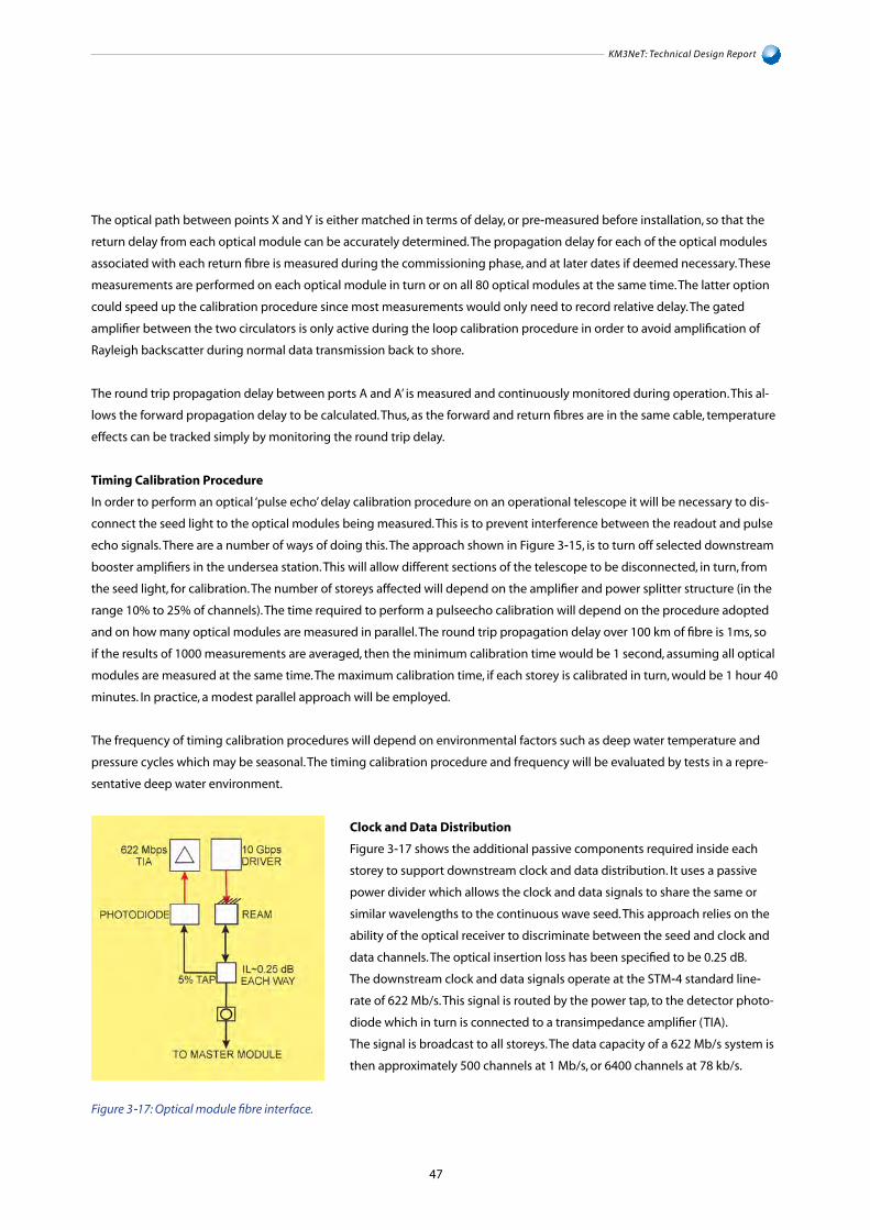
The optical path between points X and Y is either matched in terms of delay, or pre‐measured before installation, so that the
return delay from each optical module can be accurately determined. The propagation delay for each of the optical modules
associated with each return fibre is measured during the commissioning phase, and at later dates if deemed necessary. These
measurements are performed on each optical module in turn or on all 80 optical modules at the same time. The latter option
could speed up the calibration procedure since most measurements would only need to record relative delay. The gated
amplifier between the two circulators is only active during the loop calibration procedure in order to avoid amplification of
Rayleigh backscatter during normal data transmission back to shore.
The round trip propagation delay between ports A and A’ is measured and continuously monitored during operation. This al-
lows the forward propagation delay to be calculated. Thus, as the forward and return fibres are in the same cable, temperature
effects can be tracked simply by monitoring the round trip delay.
Timing Calibration Procedure
In order to perform an optical ‘pulse echo’ delay calibration procedure on an operational telescope it will be necessary to dis-
connect the seed light to the optical modules being measured. This is to prevent interference between the readout and pulse
echo signals. There are a number of ways of doing this. The approach shown in Figure 3‐15, is to turn off selected downstream
booster amplifiers in the undersea station. This will allow different sections of the telescope to be disconnected, in turn, from
the seed light, for calibration. The number of storeys affected will depend on the amplifier and power splitter structure (in the
range 10% to 25% of channels). The time required to perform a pulseecho calibration will depend on the procedure adopted
and on how many optical modules are measured in parallel. The round trip propagation delay over 100 km of fibre is 1ms, so
if the results of 1000 measurements are averaged, then the minimum calibration time would be 1 second, assuming all optical
modules are measured at the same time. The maximum calibration time, if each storey is calibrated in turn, would be 1 hour 40
minutes. In practice, a modest parallel approach will be employed.
The frequency of timing calibration procedures will depend on environmental factors such as deep water temperature and
pressure cycles which may be seasonal. The timing calibration procedure and frequency will be evaluated by tests in a repre-
sentative deep water environment.
Clock and Data Distribution
Figure 3‐17 shows the additional passive components required inside each
storey to support downstream clock and data distribution. It uses a passive
power divider which allows the clock and data signals to share the same or
similar wavelengths to the continuous wave seed. This approach relies on the
ability of the optical receiver to discriminate between the seed and clock and
data channels. The optical insertion loss has been specified to be 0.25 dB.
The downstream clock and data signals operate at the STM‐4 standard line‐rate of 622 Mb/s. This signal is routed by the power tap, to the detector photo-
diode which in turn is connected to a transimpedance amplifier (TIA).
The signal is broadcast to all storeys. The data capacity of a 622 Mb/s system is
then approximately 500 channels at 1 Mb/s, or 6400 channels at 78 kb/s.
Figure 3‐17: Optical module fibre interface.
47
KM3NeT: Technical Design Report

KM3NeT: Technical Design Report
48
The passive power tap approach to distributing clock and data, shown in Figure 3‐17, was originally devised for a dual‐input
AWG filter in the master module, however, such filters are not standard components off the shelf (see later section on DWDM
filter technology). The power tap approach requires the photo‐receiver to discriminate between the clock and data signal and
the readout seed and timing calibrations signals. The readout seed signal is more easily dealt with as this is unmodulated,
but in practice, it is unlikely that the receiver can be active during the timing calibration procedure.
Optical Amplification
Submarine quality 980 nm pumps are now available with power greater than 600 mW and failure rates of less than 25 FIT.
A system with 16 pumps at 600 mW corresponds to 9.6 W of available power. The total required signal amplification power per
bank of 20 fibres is 1.6 W. This will require approximately half of the available pump power. So, it is possible to run each pump
at half power, to improve reliability still further. The complete down‐stream booster amplifier array would require 64 pumps in
total. The overall amplifier availability remains high if any single pump fails. The total electrical power required would be less
than 100 W, assuming good heat‐sinking to sea temperature.
DWDM Filter Technology
A key requirement is that the readout should use standard components off the shelf (COTS) wherever possible. This has a
significant impact on the practicable choice of filter technology for the DWDMs. Standard telecommunications filters are
available for optical channel spacing of typically 50 GHz, 100 GHz or 200 GHz and are usually limited to about 80‐channels, al-
though an 88‐channel unit has recently appeared on the market. The narrower channel spacing filters (< 100 GHz) tend to use
active temperature control (heaters) to lock them to the ITU grid, whilst the larger channel spacing filters are usually available
in a‐thermal packages. In principle, the 50 GHz 20‐channel filters could be supplied in customised a‐thermal packages, how-
ever, the near constant operating temperature of the master module means that temperature control may not be necessary.
Based on the above assessment and an optical signal to noise ratio (OSNR) analysis, the DWDM filters employed in the master
modules are based on 20‐ channel Gaussian AWGs. Custom a‐thermal units are being investigated.
Table 3.8: Optical power budget for the passive power divider approach to clock and data distribution. This power budget is for a
specific choice of splitting and without amplification (see text).
Parameter value notes
P AWG o/p ‐10 5 Equivalent to continuous wave signal
Fibre losses ‐0.5
Connector losses ‐1.0
OM Tap ‐13 5 5% tap + 0.5 dB
Pr clock/data ‐25 5 dBm
Pr Cw ‐25 5 dBm
Total P ‐25 5 dBm
Ip 5.6 μA used to estimate MAX3658 added input referred noise
ER 3.0 linear ‐defined as P(1)/P(0)
Penalty 2.0 linear ‐defined as (ER+1)/(ER‐1)
Penalty dB 3.0 dB
Added noise penalty 2.0 dB estimate based on graph of input referred noise MAX3658
Total penalty 5.0 dB
Net Rx sensitivity ‐28.0 dBm based on MAX3658 (‐33dBm)
Margin 2.5 dB

Figure 3‐18: 10 Gb/s systems measurements over 80 km of standard fibre: Left, Dynamic Insertion Loss; Centre, Reverse bias;
Right, Extinction Ratio.
REAM Selection
The measured system parameters of the REAM, optimised for operation at 1550 nm, are shown in Figure 3‐18. The key
parameters are the wavelength dependence of the REAM’s dynamic insertion loss, on‐off extinction ratio, and bias voltage.
The curve on the left in Figure 3‐18 shows the measured dynamic insertion loss as a function of wavelength. It decreases from
a maximum of 7.5 dB at the short wavelength end of the spectrum to about 5.5 dB at the longest wavelength.
The optimum REAM bias voltage and data drive amplitude increases with wavelength, whilst the on‐off extinction ratio falls
with increasing wavelength (See also Figure 3‐18).
An 80‐channel 50 GHz DWDM requires a slightly larger wavelength range (1530 nm to 1565 nm). This extended wavelength
range means that higher bias and drive voltages would be required in order to compensate for the standard devices lower
extinction ratio at longer wavelengths.
The dynamic insertion loss has the greatest impact on system performance in the DWDM‐PON architecture and should
therefore be kept as low as possible. In order to reduce the dynamic insertion loss and the bias voltage range two versions of
the REAM are employed: one optimised for short and the other optimised for long wavelengths. In addition to improving the
optical system performance, colour banding will also simplify the REAM driver arrangements. At lower modulation
bandwidths (up to 1 Gb/s) REAM colour banding may not be necessary. Optical Signal to Noise Ratio.
The OSNR calculations for the readout architectures shown in Figure 3‐15 have been made. The noise figure for the optical
amplifiers has been set to a conservative value of 6 dB and all of the loss values are assumed to be worst case values, so confi-
dence in the real system attaining the calculated performance is very high.
The output OSNR is found to be just over 21 dB. An OSNR of 16 dB provides a theoretical bit error rate performance of 10‐9.
There is thus ample margin for the low level of transmission impairments (< 2 dB) expected in this system. Raman fibre am-
plification is precluded at distances greater than 20km. The OSNR calculations for the pulse‐echo ranging system yield similar
results Optical Power Budget.
The optical power budget calculations are summarised in Table 3.8.
A commercial trans‐impedance receiver, the Maxim MAX3658, is used as it has been designed for poor extinction ratio signals
that introduce a power penalty. In this case the power penalty is < 5 dB, giving a worst‐case operating margin of 2.4 dB.
49
KM3NeT: Technical Design Report

KM3NeT: Technical Design Report
50
This is based on the current design of the network, using a 5% power tap in the OM and the specifications of the MAX 3658
Trans Impedance Amplifier. Options to increase this optical margin are:
• Optimization of the extinction ratio, e.g. by using another ratio between CW and Clock/Data signal
• The use of a power splitter with e.g. 10% split ratio (this increases the optical power on the PIN detector in the OM but
preserves the extinction ratio)
• Addition of optical amplification in specific sections of the architecture.
Technical aspects of these options will be studied during the detailed design activities for the KM3NeT architecture and final
calculations of the optical parameters.
Backup System for Data Transmission
The architecture of the backup detection unit backbone consists of a “daisy chain” unidirectional optical path, as shown in
Figure 3‐19. Control information arrives from shore to the detection unit on a fibre going directly to the highest node of the
chain. The serial stream is transmitted with a synchronous protocol that embeds clock, slow control and data. Each node ex-
tracts the clock from the stream and regenerates it locally in order to minimize the timing jitter. Each node of the chain
handles the data‐load of all the connected nodes. It receives the stream from the previous node extracts its own data and
transmit all data including its own to the next one.
Since each node communicates only with adjacent nodes, the backbone can be implemented with single tracts of fibre driven
with “Black and White” (B&W) transceivers, which are lower cost items than DWDM lasers. The distance between storeys is
40 m and signals are regenerated at each storey, therefore the optical power budget is not an issue, allowing for the use of
cheap and standard connectors and cables.
A potential drawback is that, if a single node fails in the chain, the data transmission is interrupted causing the loss of the
whole detection unit. In order to overcome this single‐point‐failure an optical switch is used to bypass the faulty node. This
mechanism is such that even in the case of failure of all but one node, this node is still able to communicate with the second-
ary junction box. The switches are activated through a slow control system that transmits via the power line. The possibility of
bypassing many consecutive faulty nodes with semi‐passive optical devices is important in terms of reliability.
Figure 3‐19: Schematic view of the optical daisy chain architecture.

In order to further increase the backbone reliability and the overall data bandwidth, the detection unit is served by two sepa-
rated backbones, one for even and the other for odd storeys. The data rate of each single backbone is 2.5 Gb/s. With the total
rate of 5 Gb/s the readout requirements of the detection unit are met. This architecture has as many data streams as back-
bones and each backbone can be assigned a colour for data transfer to shore.
3.2.3 Network Functionalities
The design of the on‐shore DAQ system proposed here is independent of the actual implementation of the deep‐sea readout system
[14]. The design is guided by the following requirements:
• accommodate the bandwidths of any of the optical module designs;
• flexibility for implementation of any event selection algorithm;
• scalability with the use of off the shelf components.
Data Acquisition (Aggregation)
The data from each storey is routed on shore to its individual receiving port. Multiple receiving ports form the input to a con-
centrator, a unit that aggregates the data of a subset of the telescope in a single contiguous memory. This concentrator has
several output ports. In addition to aggregation, a concentrator unit is able to perform data integrity checks and decodes and
formats the data. As the data in the concentrator corresponds to a small part of the detector a filtering process can run at this
stage providing a first level of data reduction. The number of storeys a concentrator unit can handle is determined foremost
by the number of receiving ports, which in turn is matched to the size and speed of the internal memory, the processing
power and the number and speed of its output ports. The concentration ratio, i.e. the ratio of the number of input to output
ports, also depends on these factors, but will likely be in the order of 20 such that the data of all optical modules of an entire
Detection Unit can be handled in one concentrator.
Data Routing (Coalescence)
The data are routed from the concentrators via the buffer system to the processing farm and from there to the data base and
archiving systems. The routing takes place through a dedicated switch fabric. Data links from each concentrator are routed
into the buffer system, available to any processing unit within the computing cluster. The total number of output ports on the
concentrator units matches the total number of inputs to the buffer system. In case of mapping all optical modules
per detection unit to a single concentrator, the number of links to the buffer system is of order × , where is the
number of output ports of a concentrator and is the number of detection units.
The buffer system acts as an intermediate stage prior to routing any data to the processing farm. The buffer system decouples
the input data flow to the concentrators from any network congestion and latencies in the switch fabric. A processing unit can
request data from the buffer system trough a separate dedicated switch fabric.
Data Processing (Event Building)
The data is gathered as a snapshot or timeslice. Each of these is processed in an individual processor within a large computer
cluster. A snapshot covers a time span of 10‐100 ms. A central control process allocates a time slice to a given processing unit.
This unit in turn requests data from the buffer system and aggregates the data from the whole telescope for this time slice in
its own memory. Thereby, a single processing unit acts on a snapshot of the whole telescope and is able to build events based
on triggering and selection algorithms for the whole telescope. The algorithm used to process a time slice can be modified by
receipt of an external alert from other earth‐ or space‐based observatories.
51
KM3NeT: Technical Design Report

KM3NeT: Technical Design Report
52
Data Storage
The on‐shore DAQ system has three types of storage.
• Transient storage that is inherent when buffering the data at various stages. This is performed during filtering, prior to routing
the data and during processing.
• Temporary storage that is used locally to store in the shore station while it awaits transfer to final permanent storage facility.
• Permanent storage for data and data base storage.
(a) Transient Storage
Transient storage, associated with memory (RAM), occurs in the buffer system and in each of the processing units. The storage
capacity envisaged for the buffer system will be large enough to accommodate the data from the whole telescope in several
hundred time slices. Similarly the memory of each processing unit will be large enough to store the data for a few time slices.
The storage system can also be dynamically configured to handle special operations such as calibration without stalling the
data acquisition.
(b) Temporary Storage (Archival on site)
Storage on non volatile media, or the first archival of data happens at the shore station with subsequent transport of the data
from the shore station to the permanent data storage facilities. Archiving of event data and the data base is part of the critical
data path and the temporary storage system on‐site is able to keep days worth of data before transfer to permanent storage is
necessary.
(c) Permanent Storage (Final archiving)
The output from each processing unit is the raw data of a time slice that passed event selection criteria together with a set
of event description data, called meta‐data. The event meta‐data for time slices which did not pass any selection may also be
kept. For a fraction of these time slices the whole raw data may be archived to study biases and inefficiencies in the process-
ing. The data base is also stored at the permanent data storage facilities. The database will be updated for each configuration
change and after production of new calibration data.
We envisage the use of Grid concepts, as used by experiments at CERN, with a form of decentralisation for sharing comput-
ing resources in different tiers with Europe‐wide (worldwide) distribution. All data from the shore station have to be copied
to other remote facilities. A guiding principle is to ensure two copies of all data to be secure against accidental loss. A remote
facility will provide permanent storage with access to primary processed versions of the data and the capability
for reprocessing.
Control and Monitoring
Data taking will be managed by a single unit called the run control server unit. Monitoring the progress of data taking and
processing, the state of the telescope (slow controls) and the state of each individual DAQ unit will be provided by a dedicated
monitoring unit. Whereas only one run control instance will be in charge during data taking, the monitor unit will be able to
serve multiple concurrent instances for collaborators to follow the telescopes operations.

3.2.4 DAQ Model
The DAQ model covers the distributed operation sequencing logic of the telescope’s data acquisition. It is typically represented as a
finite state machine, each state corresponding to a well‐known, detector‐wide situation in which the allocation of all resources (mem-
ory buffers, processes, network connections, etc.) is exactly determined; in this picture, the state transitions are associated with the
set of operations that allocate or release these resources.
Figure 3‐20: DAQ model hierarchical state machine.
The global system can be seen as a collection of hierarchically organized subsystems that are dynamically instantiated (or destroyed)
during state transitions. Consequently, subsystems will behave only according to a subset of the global DAQ state machine, which calls
for a hierarchical representation of the DAQ Model.
Typically, the operating sequence of the detector will include a configuration selection sequence, followed by the actual configuration
of the distributed hardware and software modules, followed by the run start. This and the hierarchical organization of the subsystems
yields a state machine shown in Figure 3‐20.
The state machine transitions will be triggered by the specified events (switch, load, etc.) issued by the “run control” process. All control
processes of the different detector modules will have to implement this state machine and respond to the events issued by the central
run control.
This behaviour will be implemented through a “distributed state machine software framework” that will ensure state synchronization
between the controllers of all detector modules and will be developed using a distributed, multi‐language CORBA‐like middleware
such as ZeroC Ice with a hierarchical state machine specification framework such as CHSM.
In order to archive data efficiently, the run control programme will start a new data taking run regularly (typically every 2‐5 hours).
The configuration and control of the telescope will be managed via a user interface that allows the user to specify hardware nodes,
devices and registers using a static configuration. A central server allows for interfacing in several programming languages. Each com-
ponent in the system can be controlled and configured using a graphical user interfaces (GUIs) that can be developed using highlevel
programming languages. The configuration data are stored a priori in and retrieved from the central database.
53
KM3NeT: Technical Design Report

KM3NeT: Technical Design Report
54
3.2.5 DAQ software and firmware
The DAQ firmware includes all reprogrammable electronics implemented on FPGAs throughout the detector. The DAQ
software includes all programs running on standard workstations (onshore) and embedded platforms (offshore), including
microcontrollers. The DAQ firmware and software cover functions relating to detector and instrumentation control, configura-
tion and readout, data transmission and routing, data filtering and storage, configuration management. Table 3.9 shows
where firmware and software implementations are indispensable, possible (depending on technological choice) or not
needed.
Implementation choice
A number of architectural and technological choices will have important consequences for the implementation in software
and firmware. This choice depends on whether the readout and control and configuration intelligence is implemented entirely
in firmware or with some additional software over a system‐on‐chip platform. A system‐on‐chip solution allows for a flexible
offshore subsystem and eases the development process especially for the integration of modules developed by different
laboratories.
Table 3.9: Firmware and software implementations of main DAQ functions.
Firmware or software data routing
The detector is partitioned into subsets representing logical units of data flow to be processed onshore by a corresponding
data routing processor (e.g. one detector unit processed by one routing processor on shore). Each of these routing processors
will handle multi-gigabits per second data flow to be routed through standard Ethernet switching to the filtering farm units.
This high-performance processing can be implemented either in firmware of software. The software solution has the advan-
tage of higher flexibility and easier development but its feasibility depends on the possibilities of multi-gigabits per second
Ethernet I/O on standard workstations, either using specialized components of the shelf boards or multiple Gigabit Ethernet
boards. A firmware implementation has the advantage of higher performance and can probably allow for more compact
lower consumption electronics.
Implemented functions
Control/configuration of frond end chips
Primary readout of front-end chips
Control/configuration of PMT and instrumentation
Primary readout of instrumentation
Data transmission (over network)
Data routing
Data filtering
Data storage
l=indispensable l =possible ×=not needed
Offshore
Firmware
l
l
l
l
l
l
×
×
Software
l
×
l
l
l
l
l
l
Onshore
Firmware
×
×
×
×
l
l
×
×
Software
l
×
l
×
l
l
l
l

3.2.6 Persistency and database
Three types of data will have to be stored on persistent media:
• PMT acquisition data
• Control and configuration data
• Instrumentation acquisition data
Storing them in the form of flat files or through the use of a database server depends on the amount of data and the type of process-
ing required. The persistency model must also take into account the detector production process, including production test bench
data and integration processes taking place over multiple sites in parallel.
PMT acquisition data
This kind of data constitutes the main bulk of all the data produced by the experiment. It is organized in “runs”, each run being as-
sociated with the run conditions in which the data have been acquired. Past experience has shown that such large amounts of data
are handled with better performance over “flat” files, possibly using specialized high performance file I/O software frameworks such
as ROOT I/O. For this kind of data, only the corresponding metadata should be stored in the experiment database, using potentially
complex relations between the different elements of data description.
Control and configuration data
Configuration data is typically stored on a relational database because of the complex inter-data relationships. This kind of data
describes the hardware setup and the values of all the parameters with which this setup has been configured before producing its
acquisition data. The hardware setup can be the actual detector or any test bench or other hardware subsystem being integrated on
a production site. The control and configuration data must be time tagged and associated with the corresponding acquisition data
in a non modifiable way. At the same time, it has to be structured in a way that makes it intelligible to those who operate the detector
and those who analyse data. It has to be accessible in parallel from multiple production and science analysis sites. These requirements
lead to the persistency model described in Figure 3-21. A consequence of this model is that all access to the database goes through a
“configuration server” taking charge of:
• Metadata management
• Configuration history
• Run conditions management
• Multiple programming languages access
• Caching
• Database access performance
Software activities during the design study have produced the CConfig framework which implements all these characteristics.
Configurations are defined as sets of tree structures, automatically mapped over Oracle or MySQL database tables and automatically
support configuration history. The configuration server API is accessible in C++, Java, Python, C#, Ruby, PHP and Objective-C.
Instrumentation acquisition data
The main example of this kind of data is acoustic positioning data. These data can represent an important amount of data and are
therefore stored in flat files for raw data and database storage for metadata. The data from low data volume instruments are stored
directly in the database.
55
KM3NeT: Technical Design Report

KM3NeT: Technical Design Report
56
In thiscase, it is preferable to go through the proxy server. They can even be stored as CConfig structures, in which case they
can be handled directly by the “Configuration server.”
Figure 3-21: Persistency model.
3.3 Detection unit structure
As discussed in section 2.1 there are three options for the detection unit structure. All common considerations are presented
first, followed by the specifics of the three options. The hydrodynamic behaviour of the detection units (including those of
their anchors and dead-weights) are presented.
3.3.1 Common Issues
Many of the items in the subsystems are common to all design options.
Vertical Backbone
The link medium for bidirectional data transfer and power distribution is termed the Backbone. As discussed in Section 3.2, op-
tical transfer of digital data will be used between the storeys and the shore station. The preferred solution is a point-to-point
connection with a backup option based on a daisy chain connection scheme.
In the point-to-point data transmission scheme each storey is connected via a bidirectional mono-mode fibre to a DWDM
multiplexer in a master unit, placed at the ninth storey (counting from the anchor) of the detection unit. The DWDM unit splits
the 20 wavelengths of laser light, generated on shore and arriving via the input fibre, sending a unique wavelength to each
storey. There the light is modulated by the digitized and serialized storey data and reflected back to the master module. Here
the data from all storeys are combined onto a single output fibre. By placing the master module on the ninth storey, the lower
half of the cable contains nine bidirectional fibres together with the input and output fibres, making a total of eleven.
The upper half contains eleven bidirectional fibres. One bidirectional fibre is branched out of the cable at each storey.
The cable also carries power, at 400 V, via copper conductors. The use of two conductors, each with a cross sectional area of
1 mm2, leads to a voltage reduction at the top of the detection unit of around 3% assuming a power consumption of 15W per
storey.

At each storey the power conductors are branched out. Only the input and output fibre and the power conductors are connected to
the deep-sea network.
The key issue in the design of the backbone cable is the method for breaking out the fibre at each storey. This can be done by con-
necting sections of conventional deep-sea cable, with fibres protected in stainless steel tubes, to pressure resistant containers. Inside
the containers one fibre is connected to a bulkhead dry-mateable connector whereas the through-going fibres are fusion-spliced to
the fibres of the following cable section.
The cable can have an outer strength member if the particular detection unit design calls for this. This method was used successfully in
the ANTARES experiment, where the electrical and optical backbone was combined with mechanical functions in a single inter-storey
cable, deployed in more than 300 segments.
An alternative developed in cooperation with SEACON® is the use of a pressure-balanced oil- filled cable, in which the fibres and cop-
per conductors operate under the ambient hydrostatic pressure. This system has two distinct advantages: the cable is made in one
piece so that no fusion splicing is necessary and connector and breakout housings do not need to withstand the hydrostatic pressure.
This can lead to a significant cost reduction and simplification of the breakout design.
In the case of the daisy-chain solution, two input fibres run to the top of the detection unit. One fibre enters and exits the even num-
bered storeys, the other the odd numbered storeys. At each storey the data is added to the data stream. The monochromatic signals
are received and regenerated at each storey. In this scheme four fibres run along the length of the detection unit. At each storey two
fibres are branched out and in. At each storey power conductors are also branched out. These cables can be produced in sections with
dry-mateable connectors at each storey allowing for the breakout and power branching.
Pressure Balanced Oil Filled Backbone
Tests have been performed on a prototype oil-filled cable system. In order to keep the length manageable, 100 m of hose with three
breakouts were produced. The hose was filled with Dow Corning DC200 oil which at 40 MPa has a density of 950 kg m-3. The hose
contained four copper conductors (type 18 AWG with a cross sectional area of 0.82 mm2) and forty Corning Vascade® Leaf® fibres
with a CPC8 coating. Stainless steel containers were used for the breakout units. To each of these an oil-filled breakout cable with two
fibres and two copper conductors was connected, terminated by a SEACON® Mini-Con series connector. The backbone prototype
cable had a 40-way fibre-optic connector at either end. By interconnecting the fibres a total fibre length of almost 4 km was produced.
This system was pressure-tested at 60 MPa. No measureable deterioration of the attenuation in the fibres was observed. The copper
conductors sustained a voltage 400 V with no measureable leakage.
After conclusion of the tests the design of a production cable has begun. A specialized company (Baas BV) has produced a first feasi-
bility study. The main conclusions of this study were:
• A hose with inner diameter as small as 4 mm is possible for carrying 11 mono-mode fibres;
• The most suitable fibre is the DOW® carbon-polyamid-imid coated fibre for strength, hydrogen repulsion and size;
• The best hose material is Kynar®, as it is a plastic with superior resistance to seawater and has no plasticisers that can
dissolve in the oil;
• The hose parts can be fused to form a single system.
Siemens has recently developed a transformer-oil (Midel 7131) that has excellent ecological characteristics and has a density very
close to that of seawater (1001 kg m-3 at 40 MPa).
57
KM3NeT: Technical Design Report
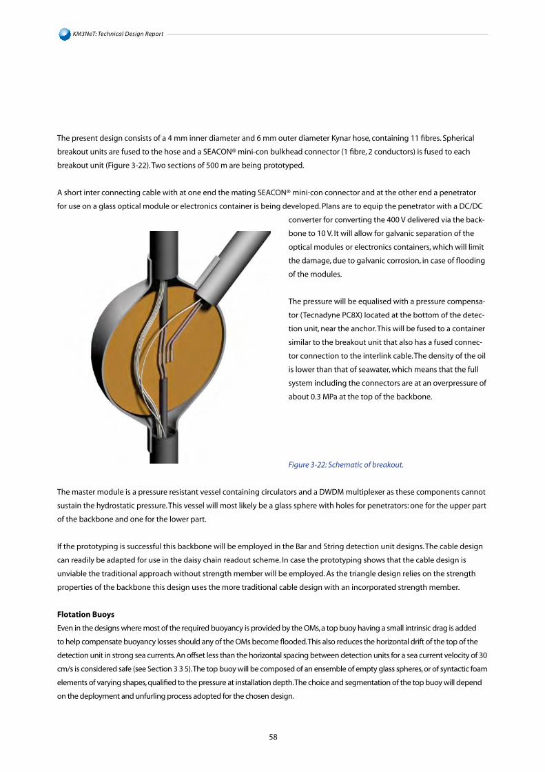
KM3NeT: Technical Design Report
58
The present design consists of a 4 mm inner diameter and 6 mm outer diameter Kynar hose, containing 11 fibres. Spherical
breakout units are fused to the hose and a SEACON® mini-con bulkhead connector (1 fibre, 2 conductors) is fused to each
breakout unit (Figure 3-22). Two sections of 500 m are being prototyped.
A short inter connecting cable with at one end the mating SEACON® mini-con connector and at the other end a penetrator
for use on a glass optical module or electronics container is being developed. Plans are to equip the penetrator with a DC/DC
converter for converting the 400 V delivered via the back-
bone to 10 V. It will allow for galvanic separation of the
optical modules or electronics containers, which will limit
the damage, due to galvanic corrosion, in case of flooding
of the modules.
The pressure will be equalised with a pressure compensa-
tor (Tecnadyne PC8X) located at the bottom of the detec-
tion unit, near the anchor. This will be fused to a container
similar to the breakout unit that also has a fused connec-
tor connection to the interlink cable. The density of the oil
is lower than that of seawater, which means that the full
system including the connectors are at an overpressure of
about 0.3 MPa at the top of the backbone.
Figure 3-22: Schematic of breakout.
The master module is a pressure resistant vessel containing circulators and a DWDM multiplexer as these components cannot
sustain the hydrostatic pressure. This vessel will most likely be a glass sphere with holes for penetrators: one for the upper part
of the backbone and one for the lower part.
If the prototyping is successful this backbone will be employed in the Bar and String detection unit designs. The cable design
can readily be adapted for use in the daisy chain readout scheme. In case the prototyping shows that the cable design is
unviable the traditional approach without strength member will be employed. As the triangle design relies on the strength
properties of the backbone this design uses the more traditional cable design with an incorporated strength member.
Flotation Buoys
Even in the designs where most of the required buoyancy is provided by the OMs, a top buoy having a small intrinsic drag is added
to help compensate buoyancy losses should any of the OMs become flooded. This also reduces the horizontal drift of the top of the
detection unit in strong sea currents. An offset less than the horizontal spacing between detection units for a sea current velocity of 30
cm/s is considered safe (see Section 3 3 5). The top buoy will be composed of an ensemble of empty glass spheres, or of syntactic foam
elements of varying shapes, qualified to the pressure at installation depth. The choice and segmentation of the top buoy will depend
on the deployment and unfurling process adopted for the chosen design.

Sea-Floor Interlink cable
This EO cable connects the detection unit base to a primary or secondary junction box. All the designs propose, during deployment,
to accommodate this cable wound on a reel fixed to the detection unit anchor. The free end of the cable terminates in a wet-mateable
connector of a hybrid (electro-optical) type or in a pair of wet-mateable connectors, one electrical and the other optical. The unwind-
ing of the reel and the connection to the junction box will be handled by a ROV.
The other end of the interlink cable is connected to the detection unit, through a penetrator, or if preferred, via a dry-mateable
connector.
Deployment
The deployment of the detection units will need surface boats equipped with dynamic positioning capabilities and equipment
including cranes, winches and cables. The number of detection units to be deployed in a relatively short time span requires this opera-
tion to be optimised in terms of cost, risk and duration. The use of compact detection units allows for transportation of many units on
board a single deployment vessel. The detection units are deployed as a compact package. This concept method has advantages in
terms of risk reduction for ship personnel and material during the deployment. It also improves tolerance to rough sea conditions.
The unfurling of the compact units is either autonomous, triggered acoustically any time after the deployment, or active using traction
provided by a winch. An advantage of delayed unfurling is that it allows for connection of the detection units to the junction box and
testing, while they are still compacted. In the event of malfunction recovery for repair is possible.
3.3.2 The Bar detection unit
The general description of this design has already been given in section 2. This section gives complementary details on this design
option. The mechanical structure of the detection unit is a semi-rigid system composed of a sequence of horizontal elements (storeys)
interlinked by a system of tensioning ropes arranged to force each storey to a position perpendicular to its vertical neighbours. The
detection unit is anchored on the seabed. A buoy located on top of the structure provides the pull to keep the structure vertical and
ensure its rigidity.
The storeys support the optical modules and the pressure
vessels for the local storey electronics as well as the ancil-
lary instrumentation needed (hydrophones for the acoustic
positioning system, environmental probes, etc.).
Figure 3-23: The packed detection unit.
59
KM3NeT: Technical Design Report

KM3NeT: Technical Design Report
60
Product breakdown for the bar detection unit.
Component Description Quantity
Anchor Carbon steel structure to provide weight to keep detection unit 1
on seafloor.
Detection unit base Releasable metal structure forming connection between anchor 1
and mechanical ropes.
Storey Mechanical structure with optical modules and electronics container. 20
Mechanical ropes Dyneema™ ropes, 4 mm diameter, running the full length of the 4
detection unit. Supporting and orienting the storey. Length 900 m.
Backbone cable Oil filled vertical cable providing power and fibre optic 1
connectivity from detection unit base to the storeys.
A dry mateable connector one fibre and two conductors at
each storey.
Backbone master Pressure resistant vessel containing DWDM unit and optical 1
module circulator circuitry.
Floatation system System of buoys at top of detection unit to keep it upright. 1
Interlink cable Cable with two fibres and two copper conductors, dry mated to 1
detection unit and with wet mateable connector at other end.
Length as required by layout.
Product breakdown of storey.
Component Description Quantity
Optical module Described in Chapter 3.1.2 6
Electronics container Described in Chapter 3.1.2 1
Storey structure Aluminium structure 6 m x 0.4 m to support optical modules 1
and electronics container.
Table 3.10: Product breakdown of Bar detection unit.
Anchor
A disposable anchor at the bottom of the structure provides the
weight needed to anchor the detection unit on the seabed. This
anchor is an anode-protected carbon steel trellis with length equal
to that of the storeys (Figure 3-24).
During the integration, transport and deployment stages this
structure also provides the support for the compact package of
storeys.
The dimensions and characteristics of the detection unit
anchor are given in Table 3.11. Figure 3-24: The detection unit anchor.

Base Unit
Length (m) 5.8
Width (m) 0.46
Height (m) 0.5
Mass (kg) 65
Net buoyancy in water (N) ‐450
Buoy
Length (m) 5
Width (m) 1.6
Height (m) 0.4
Mass (kg) 1500
Net buoyancy in water (N) 10000
Anchor
Length (m) 6
Width (m) 2.55
Height (m) 0.5
Mass (kg) 3000
Net buoyancy in water (N) ‐25600
Storey
Length (m) 6
Width (m) 0.46
Height (m) 0.43
Mass mechanical structure (kg) 55
Mass including OM and 115
electronics container (kg)
Net buoyancy in water (N) 300
Table 3.11: Bar detection unit characteristics.
Base Unit
The detection unit base (Figure 3-25) is a trellis structure built in series 5000 corrosion-resistant aluminium and attached to the anchor
by means of an acoustic release system. It provides the link between the anchor and the vertical sequence of storeys.
The lower ends of the tensioning ropes linking the first detection unit storey are connected to this structure.
Figure 3-25: The detection unit base structure.
61
KM3NeT: Technical Design Report

KM3NeT: Technical Design Report
62
Storeys
The storeys (shown in Figure 3-26) are 6 m long mechanical bar structures in series 5000 Aluminium which support the OMs and the
ancillary equipment.
The exact position and orientation of OMs on the storey will be defined following the results of simulations. The present hypothesis
foresees three pairs of OMs, each housed in a 13 inch glass sphere. Two pairs are located at the ends of the bar, with one OM looking
outwards and one looking downwards, while a third pair is located in centre of the storey, with the two OMs looking out perpendicular
to the bar at 45° downward from the vertical.
Figure 3-26: The storey for the Bar detection unit.
Dimensions and characteristics of the detection unit storey are given in Table 3.11. A sketch is presented in Figure 3-26.
The link between adjacent storeys is provided by means of a system of 4 mm Dyneema® ropes. These are fixed in pairs at each storey
corner so that the set of two storeys and four ropes can assume a tetrahedral shape, as shown in Figure 3-27.
Figure 3-27: A few of storeys with interconnecting ropes for the Bar detection unit (vertical scale is reduced).
The configuration of the ropes forces the two storeys into a perpendicular orientation with respect to one another and gives structure
rigidity against torsion.

Flotation Buoy
The flotation system is composed of a set of cylindrical syntactic foam floaters interconnected with aluminium plates in a rigid
package.
Figure 3-28: The flotation system for the Bar detection unit.
The flotation system is connected to the upper storey of the detection unit by ropes of the same type as those used for the inter-sto-
rey interconnection.
Dimensions and characteristics of the flotation system are given in Table 3.11
“Bar” design: Deployment
For deployment the detection unit is a compact package with the shape of a parallelepiped and size of 6 x 2 5 x 2.5 m. This package
has to be deployed and positioned at depths beyond 2500 m.
The final working configuration will be reached, after deployment and connection of the structure, by remotely actuating an acoustic
release system. The unfurling of the structure will be driven by the pull of the top buoy.
The operation sequence is the following:
• Lifting of the structure on the ship deck. This operation is performed using the ship’s deck equipment.
• Immersion of the structure in the water. This operation is performed using the ship’s deck equipment.
• Lowering of the structure close to the seabed. This operation requires a winch hosting a cable length sufficient for the site depth.
• Positioning of the structure on the seabed. The required accuracy (order of few metres) require the availability of an acoustic
Long Base Line (LBL).
• Release of the structure. This operation will be performed by remotely actuating an acoustic release system placed at the end of
the deployment cable.
63
KM3NeT: Technical Design Report

KM3NeT: Technical Design Report
64
Table 3.12: Product breakdown for the String detection unit.
3.3.3 The String detection unit
The general description of this design has already been given in section 2 and in Section 3.3.1. This section gives complementary
details on this design.
The “string” detection unit is a lightweight structure of 20 storeys each comprising single OMs of the Multi-PMT type spaced verti-
cally 30 m apart (see Figure 3-29). The structure is designed to have minimal hydrodynamic drag. The mechanical and electro-optical
structures are separated, the former being provided by two ropes and the latter by a separate backbone cable. The detection unit is
held on the seafloor with a deadweight connected to the ropes. The detection unit is held vertical mainly by the buoyancy of the OMs
and in addition by extra buoyancy of the top buoy. Each OM is a self-contained unit whose failure does not influence the working of
the remaining ones. OMs are connected to the vertical ropes at regular intervals via individual connection rings. The electro-optical
backbone cable is an oil-filled equipressure cable that contains a fibre per OM together with two electrical conductors for the power
distribution throughout the detection unit. The backbone has a branch out of an optical fibre and two electrical conductors at each
OM. The connection from the base of the detection unit to the seafloor network passes via an electro-optic interlink cable terminat-
ing in a hybrid (EO) wet-mate connector for connection to the seafloor network. This interlink is an extension of the backbone cable
containing two optical fibres and two electrical power conductors. The interface between the two unidirectional fibres to and from
the seafloor network and the bidirectional fibres to each OM is placed within a “master module”, a pressure vessel that contains the
circulator and DWDM multiplexer (section 3.2.2)
The product breakdown for the detection unit is given in Table 3.12.
Product breakdown for the bar detection unit.
Component Description Quantity
Anchor Concrete deadweight to keep detection unit on seafloor. 1
Storey Mechanical structure with optical module. 1
Mechanical ropes Dyneema™ ropes, 4 mm diameter, running the full length of the 2
detection unit. Supporting and orienting the storey. Length 700 m.
Backbone cable Oil filled vertical cable providing power and fibre optic 1
connectivity from detection unit base to the storeys. A dry mateable
connector for one fibre and two conductors at each storey.
Backbone master Pressure resistant vessel containing DWDM unit and optical 1
circulator circuitry.
Floatation system System of buoys at top of detection unit to keep it upright. 1
Interlink cable Cable with two fibres and two copper conductors, dry mated to 1
detection unit and with hybrid wet-mateable connector at other end.
Length as required by layout.
Product breakdown of storey.
Component Description Quantity
Optical module Described in Chapter 3.1.2 6
Electronics container Described in Chapter 3.1.2 1
Storey structure Aluminium structure 6 m x 0.4 m to support optical modules 1
and electronics container.

Anchor
The anchor in the string detection unit is a dead-weight to
which the vertical mechanical ropes are connected. It will
be constructed of concrete. Between 0 5 and 1 m3 will be
required. The weight in air of 1 m3 of concrete is 2400 kg and
therefore the negative buoyancy in water is 13240 N.
Mechanical Structure
The mechanical structure consists of two 4 mm Dyneema®
ropes running the full length of the structure. The ropes will
be delivered with length markings. The markings are made
while the ropes are tensioned at the full tension expected
during operation in the sea. At regular intervals thin Dynee-
ma® strings are inserted through the ropes for attaching the
electro-optical backbone cable.
Storey
For the string detection unit the storey is a single Multi-PMT
optical module as described in section 3.1.4. The single sphere
is connected to the ropes of the mechanical structure using
a spring-loaded titanium ring. The ring has two sets of four
titanium cleats. The ropes are run around the cleats and finally
capped with a titanium cap. On one side of the ring there is
also a provision for connecting the backbone cable. Figure
3-30 shows the ring structure.
Figure 3-29: Schematic layout of the String Detection Unit (from bottom at left to top at right)
Figure 3-30: The spring loaded titanium connection ring
65
KM3NeT: Technical Design Report

KM3NeT: Technical Design Report
66
Deployment
There have been several requirements formulated for the deployment of the detection unit:
• It should fit in a standard transport container, to facilitate transport to the deployment port.
• At least eight detection units should be deployed in a single sea operation of three days otherwise these become prohibitively
expensive both in time and money.
• These requirements have resulted in a number of restrictions on the deployment techniques:
• Deployment must proceed at least as a single unit (compact deployment)
• The detection unit must be in a compact transportable state when deployed
(inner dimensions of a 20 ft container: 5.88 x 2.35 x 2.35 m3)
• It must unfurl once on the seafloor
• Deployment frames must be reusable.
Deployment Structure
The deployment structure consists of a spherical aluminium structure (see Figure 3-31) with cable trays running round its circumfer-
ence. The diameter is 2.1 m. The three sets of cable trays run from pole to pole and are offset by 60° Between the cable trays of each
set, holes in the sphere provide the space for suspending the optical modules in the structure. The structure is loaded during assembly
of the detection unit. First the five glass buoys are loaded on guiding rails through the hole at the North Pole. The first optical module
is placed in the first hole next to the north pole and kept in place by a lever blocked by the ropes. The spherical structure is rotated
around a winding axis perpendicular to the first cable tray. The Dyneema™ ropes and the backbone cable are laid in the trays. After
five rotations the next optical module will be aligned with the next hole on the circumference and secured in it. This is continued until
all holes in this first tray set are filled. (The holes at the poles are skipped). The spherical structure is rotated around the north-south
axis by 60° to be able to fill the next cable tray set. The winding axis is changed accordingly. This cable tray is then filled followed by the
last. During the loading of the last cable tray the hole at the South Pole is also filled. The final sphere is placed at the North Pole after
which the remaining 100 m of ropes are wound round the spherical structure. The ropes are connected to the anchor. The sphere has
three tubes (not shown) running through it so that during deployment cables can run through them from a spreader structure at the
top to the anchor. In this way the deployment forces are taken by the deployment cable rather than the spherical structure.
Figure 3-31: Spherical deployment structure, design and during deployment.

The spreader is secured to the anchor by an acoustic release mechanism. When released the spreader is winched to the surface and
the structure rises due to its buoyancy. It rotates as it rises to the surface and unwinds the detection unit. When the last glass spheres
have been released the spherical structure rises to the surface under its own buoyancy. This allows for recovery and reuse. Two of these
structures fit into a 20 foot container. The deployment structure with all ancillaries takes up a deck-space of 2.2 x 2.2 m2. The units will
be transported and stored on deck, two-by-two, in open top 20 foot containers. This will protect the units during transport and facili-
tate deployment. A minimum of eight units will be transported at a time on the deployment ship.
Maintenance
Following unfurling no maintenance of detection units is planned. When predicting the global performance of the detector, account
must be taken of the probability that parts - storeys or optical modules - will become blind. The power and data network must be
designed in such a way that in no case can the failure of a detection unit propagate to another part of the detector.
3.3.4 The Triangle detection unit
The general description of this design has already been given in section 2 and in Section 3.3.1. This section gives complementary
details on this design.
The detection unit is inspired by ANTARES experience but represents an improved design in a compact string-type geometry allowing
for easy transportation and deployment with remote unfurling on the sea bed. This unfurling requires a special apparatus, termed the
“bell”. The 6 optical modules of each storey are of the large PMT type (see Section 3.1.2) with the electronics housed in extra 7th glass
sphere.
In the large PMT option, the 6 optical modules of each storey are grouped in 3 close pairs with adjacent pairs azimuthally separated by
120°. The two optical modules of each pair are used in coincidence with a PMT looking horizontally and the other looking downward,
at 45°, both in direction at the opposite of the storey axis. The storey electronics sphere is linked electrically and optically - through a
connector at one end and a penetrator at the other - to the backbone. The six OM spheres, each containing only a PMT and HV base,
are linked electrically - through a connector at one end and a penetrator at the other - to the electronics sphere (see Figure 3-32).
Figure 3-28: The flotation system for the Bar detection unit.
67
KM3NeT: Technical Design Report

KM3NeT: Technical Design Report
68
Table 3.13: Product breakdown for the Triangle detection unit.
The storeys have a horizontal layout (overall diameter 2.5m) and, before the unfurling, they are stacked as “triplets” for compactness
(see Figure 3-33).
Figure 3-33: View of a nested pre-deployment triplet of three storeys of the Triangle detection unit.
Product breakdown for the Triangle detection unit.
Component Description Quantity
Anchor The anchor is a dead weight to keep the detection unit on the 1
seafloor. It carries the bell and the interlink mobile spool.
Storey The mechanical structure with optical modules and an 20
electronic container.
Backbone cable It is meant to keep the optical modules spaced vertically in 4
sections the water while distributing the power and the data.
At regular intervals a storey is connected to the cable mechanically
(by a pair of mechanical terminations and crow’s foot riggings) and
electro-optically (through a break out unit). Sections are connected
through dry-mateable hybrid connectors.
Backbone master Pressure resistant vessel containing DWDM unit and optical 1
module circulator circuitry.
Floatation system Buoy at top of detection unit to keep it upright. 1
Interlink cable Cable with two fibres and two copper conductors, dry mated to 1
detection unit and with hybrid wet-mateable connector at other
end. Length as required by layout.
Product breakdown of storey.
Component Description Quantity
Optical module Described in Chapter 3.1.2 6
Electronics container Described in Chapter 3.1.2 1
Storey structure A welded structure of marine aluminium alloy, connecting the optical 1
modules and the electronic container to the backbone cable.

In an alternative design each pair of OMs is replaced by a “capsule” (see Section 3.1.3) containing a pair of PMTs. In this design, each of
the 20 storeys would house 3 OM/capsules which would also contain the OM electronics, eliminating the extra sphere.
The detection unit has 20 storeys (loaded on 7 pre-deployment “triplets”, the last being incomplete) spaced 40 m apart after deploy-
ment between 100 and 860 m from the sea bottom. The backbone spaces the OMs spaced vertically in the water while providing the
power and data flow. Storeys are mechanically connected to the cable - through a pair of mechanical terminations and crow’s foot
riggings - and electro-optically through a break out unit – an electro-optical “T” connection between two adjacent cable sections and
the storey electronics.
The detection unit anchor carries the “bell”, the master module and the interlink cable
wound on its mobile reel. The master module is a pressure vessel that contains the
DWDM filter, and serves as a connection point between the backbone cable and the
interlink cable to the deep sea network. Cable entries through the wall of the master
module may use (connector-less) penetrators, or alternatively dry (surface-mate)
connectors. The distant end of the interlink cable which connects with the seafloor
network terminates in a hybrid wet-mate EO connector. The product breakdown for
the Triangle detection unit is given in Table 3.13.
Figure 3-34: Triangle detection unit: detail of optical module and electronics sphere
interconnections.
Storey
The mechanical structure of the storey is made of welded marine aluminium alloy (Titanium and composite material are also consid-
ered) with the following functions:
• to support the 6 OMs, the electronics sphere and the break out unit;
• to mechanically connect the up-going and down-going cable segments to neighbouring storeys, the buoy or master module;
• to hold, before unfurling, the 30m long cable sections (connecting a storey to its neighbours) in a safe way, avoiding any risk of
blocking during the remote unfurling process;
• to constitute a stable stack in air as well as in water before unfurling.
The storey exhibits a 3-fold rotational symmetry around the detection unit axis. Figure 3-34 is a view of a single storey, whereas Figure
3-33 shows three consecutive storeys belonging to the same triplet stacked
together, with the three corresponding cable sections wound in the middle.
This assembly is the elementary brick of the whole stacked detection unit
(see Figure 3-35) made of 7 such bricks. Figure 3-36 is a view of a central part
of the unfurled detection unit.
• The weight in water of a storey, without the OM but with break out unit,
electronics and cable mechanical termination, is 30kg.
• In the case of accidental corrosion of the structure of a storey, the damage
will not propagate further; the mechanical, electrical and optical integrity of
the vertical backbone will be preserved.
Figure 3-35: Triangle detection unit in stacked configuration with 20 storeys.
69
KM3NeT: Technical Design Report

KM3NeT: Technical Design Report
70
Anchor
The anchor is a heavy plate of anode-protected steel (or of concrete) having a weight in water of about -30000N (cf. Section 3 3 5). In
addition, it carries the master module electronics container, the interlink cable reel, the acoustically triggered unfurling system and the
bottom section of the vertical cable.
Buoyancy
Most of the detection unit’s buoyancy is provided by the storeys but a top buoy is still needed to reduce the detection unit inclination
in the case of strong horizontal sea currents (cf. the “detection unit stability” section). Each sphere has a buoyancy of 73 N. Taking into
account the weights of the mechanical structure of the storey, the cable sections, their mechanical terminations and break out unit
and of the electronic equipment, the net buoyancy of a storey will be 220 N. The top buoy will be a sphere of 1.4m diameter (or an
ellipsoid of the same volume), made of syntactic foam of a density around 0.6 and located 10m above the top storey.
Figure 3-36: The unfurled detection unit. Bottom, central and top section.

Horizontal Interlink Cable
The detection unit interlink cable is coiled on a reel mounted on the detection unit anchor and connected to the sea floor network
through a wet mate connector handled by a ROV. The possibility of unplugging interlink cables allows for the recovery of deep sea
junction boxes for servicing, should this become necessary.
Vertical Backbone and Strength Cable
The backbone is inspired by the ANTARES implementation of an electro-optic core protected and surrounded by a layer of Aramid
fibres under a polyurethane sheath.
The breaking load is reduced from the 180 kN ANTARES figure to around to 70 kN (still representing a safety factor of ~ 6) since the
cable does not need to support the detection unit during deployment. The maximum stress is limited to that which occurs during the
unfurling of the detection unit.
The break out is a delicate part of the backbone. A base solution under study employs a unique moulded part in which conditions
close to equipressure are achieved, through the choice of moulding material. This solution would reduce the cost and provide a barrier
at each storey as well as protection against short-circuit in the case of water ingress.
The mechanical part of the cable (the Aramid braid) ends around 1m above and below the storey in Titanium mechanical termina-
tions. From this point, crow’s feet rigging of triple Dyneema® ropes connect to the storey structure to maintain the plane of the storey
perpendicular to the cable. The electro-optic core of the cable continues up to the break out unit with some additional length which
allows the remaking of any faulty breakout at construction time and prevents accidental tensioning or over-bending of this part of the
cable at unfurling time.
Logistics
We assume a maximum allowed volume for a furled detection unit of 2.5m (horizontal diameter) x 3.5m (vertical height) for road
transportation. The bare furled detection unit (including the OMs and the base plate but without the deadweight, buoy and unfurling
bell), fits easily within this volume and will be transported by road from the integration site to the deployment harbour. There the top
buoy, the deadweight and the unfurling bell will be added and the whole assembly loaded onto the deployment boat. The foot-print
of a detection unit on the deck will be 2.7m x3m =8.1m2.
Unfurling
The stack of 20 storeys is initially held on the base within the unfurling bell. The base and the bell are linked by a rope that can be
acoustically released to permit the unfurling. The bell containing the 20 storeys rises slowly under the action of the cable/winch
system of the deployment boat. The bottom section of the vertical cable, initially wound on the base plate, is freely released during the
ascent up to a height of 100 m, where the first storey is left automatically.
On this storey the next section of cable has been wound, ready for the nest step of the lift. The process continues until all the storeys
and the top buoy are released below the bell. Then the bell continues alone, at the speed allowed by the winch, to the surface, where it
is recovered by the deployment boat for reuse.
The shock occurring along the vertical cable each time a new storey is released from the raising bell will be limited by reducing the
speed of the winch during the unfurling phase. The deployment hook will be equipped of a low friction swivel in order to avoid any
transfer of torsion from the deep sea cable to the detection unit vertical cable during the unfurling.
The bell is a heavy object (at least 1.5T of protected steel) intended to keep the deep sea winch cable under tension during detection
unit unfurling. Its centre of gravity will be significantly lower than the centre of buoyancy of the stacked detection unit inside it, in
order to ensure the up-down stability of the assembly.
71
KM3NeT: Technical Design Report

KM3NeT: Technical Design Report
72
Maintenance
Following unfurling no maintenance of detection units is planned. When predicting the global performance of the detector, the
probability that storeys and optical modules may become blind must be taken into account.. The power and data network must be
designed in such a way that in no case can the failure of a detection unit propagate to another part of the detector.
Maintenance will be ‘replaced’ by a test of the detection unit in situ while still furled (which means still connected by the winch to
the deployment boat). Several options are presently under study. In the event of failure at this stage, the furled detection unit will be
recovered with its base for repair.
The partial loss of detection unit buoyancy which might cause it to interfere with its neighbours will of course require an emergency
procedure. A ROV is needed to cut the vertical cable at a point where it is still under tension. Slow sea current conditions are manda-
tory. The released part of the detection unit is then recovered by a surface boat.
The only recovery of a detection unit after the unfurling will be during decommissioning following the end of detector operation. This
could be done from a surface boat by dredging.
Component availability
Due to the large number of parts needed and in order to reduce the procurement risk, several sources are required for each single
component. This should be easy for the mechanics, the cables and the electronics but more difficult for 3 critical parts: the glass
spheres, the PMTs and the connectors. In the building phase, the production of these parts will be followed permanently by basing
representatives of the project at the production sites.
3.3.5 Hydrodynamic behaviour
The behaviour of a generic detection unit under the effect of the sea currents is modelled considering the detection unit as a se-
quence of rigid units. Two adjacent units are supposed free to rotate around a horizontal axis perpendicular to the direction of the sea
current:
Figure 3-37: The detection unit approximated as a string of rigid units al-
lows a simple derivation of the shape from lift and drag.
In the cases of flexible detection units (String and Triangle options), a
unit is a storey (or top buoy) with the cable or ropes of various lengths
attached below the storey (see Figure 3-37).
In the case of the bar design, due to its specific rigging, the unit is the
parallelogram of Figure 3-38. It therefore consists of two adjacent
storeys and ropes; the one perpendicular and the other parallel to the
direction of the current.


3.4 Telescope Deep Sea Network
The building blocks described in the previous chapters have not at this point been optimised. The inter-unit distance has to some ex-
tent been optimised, but the layout on the seafloor still needs tuning. In addition the number of detection units in the building blocks
depends strongly on the detection unit design. The full detector, equivalent to about 2 building blocks contains about 320 bar, 280
triangle units or 650 string units. This has a consequence that the description of the seafloor network will only be possible in terms of
general architecture and operation principles rather than a full completely worked out design. The architecture that will be described
is a star network with successive branching from the main electro-optical cables to the detection units. The implementation of this
branching will depend on available technology, the efficiency of power distribution, the number of wavelengths carried on each data
transmission fibre and of course the exact layout of the detection units on the seafloor.
The power transfer from the shore to the primary junction box is performed at high voltage, of the order of 10 kV, whereas the
network from primary junction box onward operates at 375 V. The power losses in the different parts of the seafloor network have
significant implications for the overall network requirements.
3.4.1 Network Components
In general the system consists of
• Power feeding equipment;
• Main electro-optical cables: the connection of the detector to shore for power, data and control signal transmission;
• Primary junction box(es): Conversion of high voltage to medium-voltage;
• Secondary junction boxes;
• Cables between primary and secondary junction boxes;
• Interlink cables from secondary junction boxes to the detection units.
Overall Power Requirements
The power requirements are determined mostly by the detection units. Each of the 320 (650) units have a consumption of 300 W
(150 W). In addition there are power losses at the different stages of the system. The total power requ rement of the detection units
is 96 kW. The associated sciences node requires 10 kW. The additional power due to losses, predominantly in the main electro-optical
cable and the medium voltage converters, is around 30 % so that the total required power on the shore is 155 kW. (See Table 3.15)
Table 3.15: Power budget for full detector.
75
KM3NeT: Technical Design Report
Total load detection units
Interconnecting cable losses (375 V DC)
Interconnecting cable voltage drop
Associated science power
Medium-voltage converter power loss (η=80%)
Total power at deep see
Main cable loss
Total power loss
Shore power required
96 kW
4 kW
<4%
10 kW
27.5 kW
137.5 kW
17 kW
30%
155 kW

KM3NeT: Technical Design Report
76
Power Flow Scheme
The power transmission system consists of two shore based 85 kW, 10 kV DC, 8.5 A power supplies, the main electro-optical cables
operating at 10 kV DC, each with one power conductor with the return current being led through the seawater. The alternative cable
solution, with copper return will be considered should environmental laws, at the time and site of deployment, exclude operation of a
sea return. This will then have consequences both in financial and power terms.
A schematic view of power flow in the sea floor network is presented in Figure 3-39. At the end of each cable the 10 kV DC is trans-
formed down to 375 V DC for supply to the detection units. This is done using 14 10 kW medium-voltage converters. These converters
can be located close together or in principle separated so that each converter feeds a part of the detector in situ. This then requires
additional equipment to split the main electro-optical cable, that are commercially available.
Because of power losses in the medium-voltage converter a maximum of 8.0 kW of power is provided to the detection units from
each converter. The units are reached via the secondary junction boxes. A similar path is followed by the fibre optics network used for
bi-directional data transmission and control. The fibre optic network was described in section 3.2 and will not be discussed further in
this section. The only requirement stemming from the fibre network is that in the secondary junction box the communications wave-
lengths from four detection units are multiplexed onto a single fibre. The secondary junction box should therefore feed multiples of
four detection units. The description below assumes a secondary junction box connecting to eight detection units. The detection units
are designed to operate at a minimum voltage of 350 V corresponding, in the worst case, to a drop of no more than 25 V from primary
junction box to detection unit.
The primary-to-secondary junction box cables have four copper conductors, with 13 mm2 cross section each, rated for 600 V operation
and have an assumed maximum length of 1500 m leading to a voltage drop of 12.7 V; the cables running from the secondary junction
box to the detection units have four copper conductors, with 2 5 mm2 cross section each, rated for 600V operation and at a length of
400 m lead to an additional 2 2 V loss. The power lost in the cables is around 4 kW for the full system.
Figure 3-39: Power flow block diagram.

3.4.2 The Main Electro-Optical Cable
The KM3NeT site-to-shore main cables, which carry the optical fibres and electrical conductors, must survive both the rigours of
installation (torsion, tension due to its own weight and ship movement) and the seabed conditions (high ambient pressure, abrasion
risk and unsupported spans). Furthermore, the longevity of the read-out system depends on minimizing the strain induced on the
optical fibres.
Submarine telecommunication cables satisfy these requirements. They have to provide service lives of at least 25 years and they must
be easy to deploy and repair at sea. In addition, standard telecommunication cables have the advantage of working with a wide range
of industry-approved accessories (such as connection boxes, couplings and penetrators). These accessories have shown very low
failure rates and can be readily used to interface with scientific equipment. Thus the KM3NeT main electro-optical cables will be, to the
extent possible, standard submarine telecommunication cables.
The solution where submarine cables with a single copper core are used will require two cables for the full detector. Then 96 fibres in
each of the cables are necessary for the data transport.
The fibre types used for submarine transmission are optimised for minimum attenuation over the full C-band (1530-1570 nm) with
dispersion characteristics that depend on the application. The main electro-optical cable has to be equipped with standard mono-
mode fibres conforming to ITU-T standard G.655.
A single conductor power transmission system with current return via the seawater would allows for a light cable. The extremely small
resistance of the sea return also implies a system with lower power losses. Such systems must incorporate sea electrodes both at the
shore and in the deep sea. An issue with a DC single conductor system is the corrosion of neighbouring structures and installations.
The anode is placed on shore in wet ground. Provisions will be made to capture any liberated chlorine gas. At the kathode a depletion
of the H+ ions leads to a reduction of the pH of the seawater in the vicinity of the electrode. This issue will have to be addressed.
Table 3.16: Main Electro-Optical Cable characteristics.
A system providing data and power transmission over 100 km is in use between the Capo Passero on-shore laboratory and the deep
sea site at 3500m depths. The cable was manufactured by Alcatel-Lucent and deployed in July 2007. The system can be operated at up
to 10 kV DC at a power level of more than 50 kW.
The KM3NeT main electro-optical cable characteristics for the data and power transmission are summarized in Table 3.16.
There exist many kinds of submarine cable armouring. The armour is selected to be compatible with the specific cabling route on the
seafloor. The final characteristics of the main electro-optical cable will therefore depend strongly on the deployment site.
77
KM3NeT: Technical Design Report
Length [km]
Type of power to be transmitted
Maximum Voltage [kV]
Maximum Current [A]
Cable resistance [Ω/km]
Number of fibres
100
DC, sea return
10
10
1
96

KM3NeT: Technical Design Report
78
Medium Voltage Converter
At the end of the main electro-optical cable there will be a frame termination assembly that will contain:
• a cable termination assembly that separates the power and fibre optic paths;
• a system of Medium Voltage Converters;
• a patch panel with several output wet-mateable connectors.
The medium-voltage converter transforms 10 kV DC input to an output of 375 V DC. An example of such a converter is the 10 kV to
375 V DC, 10 kW medium-voltage converter built by Alcatel for the NEMO project, which in turn was based on a design developed by
JPL-NASA for the NEPTUNE project[15]. The measured efficiency is 87% at full load.
Figure 3-40: The DC/DC Medium Voltage Converter layout.
The converter is configured as a matrix of 48 power converter building blocks arranged in 6 columns connected in parallel, each
having 8 blocks in series (Figure 3-40). This arrangement allows for the converter to continue operating, even with some faults in the
printed circuit boards. Each building block is a pulse width modulated switching forward converter with an input of 200 V and an out-
put of 50 V with a capacity of roughly 200 W. Each block has four MOSFETs, two working as a primary switch and two on the secondary
side as a synchronous rectifier. A block diagram of the circuit is shown in Figure 3-41. The various transformers are able to withstand
continuous 10kV operation
Figure 3-41: The DC/DC Medium Voltage Converter PCBB block diagram.

The entire power converter is housed in a pressure vessel filled with a dielectric fluid (Fluorinert®) for cooling and insulation. The com-
plete medium-voltage converter is shown in Figure 3-42.
Figure 3-42: The Medium Voltage Converter.
The main characteristics of the medium-voltage converter, as measured on a functioning device, are shown in Table 3.17
Table 3.17: Medium-voltage converter characteristics.
79
KM3NeT: Technical Design Report
Input Voltage
Output Voltage
Output current
Input shut down voltage
Efficiency at 10kV, full load
Voltage undershoot at 10kV -10% to 90% step up
Voltage overshoot at 10kV -90% to 10% step down
Output Ripple Voltage, rms at 100 kHz
5.7 - 10 kV
375 V
25 A
5,2 kV
87%
40 V
43 V
1,5 V

KM3NeT: Technical Design Report
80
Primary Junction Box
The block diagram of the primary junction box is shown in Figure 3-43. Its main function is to route the 375 V DC power from the me-
dium-voltage converters to the secondary junction boxes. The power from the medium-voltage converters will be connected inside
the primary junction box in such a way that a secondary junction box can be fed by more than one medium-voltage converter, thus
providing redundancy. Another functionality of the primary junction box is the monitoring and control of the output lines. The prima-
ry junction box also has remotely actuated relays that connect the secondary junction box to the medium-voltage converter system,
that are used to switch on and off the feed lines during normal operation and to automatically isolate a faulty line. The bi-directional
communication of control and data between the primary junction box and the shore station is achieved via a fibre optic connection.
The primary junction box will have acoustic transponders so that its location on the sea floor can be easily determined. It must have
a highly reliable operation and also it should allow for its recovery for maintenance or replacement, since it is a point where a single
point failure may have truly severe consequences for the detector’s operation. In addition a layout that allows for easy access of an
ROV to the wet-mateable connectors is required.
Figure 3-43: Block diagram of the sea-floor power distribution chain.
The specific details of the primary junction box depend on the exact configuration of the detector to be built, and thus the primary
junction box will be one of the last components to be detailed. Both the ANTARES and NEMO projects have deployed and operated
junction boxes in the deep sea with all the required functionalities. Descriptions of the various junction boxes are given elsewhere[16].
Salient features of the NEMO junction boxes are: (i) one incorporates the medium-voltage converter described above connected to
the main electro-optical cable’s cable termination assembly via a 10 kV DC connector which is designed to be wet-mateable, and (ii)
another one makes an innovative use of an external light-weight fibreglass oil-filled tank to prevent the corrosion of inner pressure
resisting steel tanks containing the electronic components. The use of regular steel tanks rather than titanium containers allows for
a more economical structure. In contrast, the ANTARES junction box has a dry mateable main electro-optical cable connector and
employs a titanium sphere as its electronics container.

Secondary Junction Box
Each secondary junction box serves a group of 8 detection units and is located near them so that the distance to the detection units
is as short as possible. Its function is to distribute the power coming from the primary junction box to the detection units. The power
distribution network inside the secondary junction box is shown in Figure 3-44.
The secondary junction box contains:
• a power feed system able to supply all the internal loads;
• a monitoring & control system that will monitor and switch on and off the output lines;
• input and output 600 V wet-mateable connectors including some spare connectors.
The sum of conductors and fibres in each connector should not exceed 8 to allow the use of available hybrid electro-optical
connectors.
Figure 3-44: Block diagram of the Secondary Junction Box.
Examples
Just as examples of the different layouts that can be achieved using the architecture described above two options that could be used
to power the building block are described in the following.
81
KM3NeT: Technical Design Report

KM3NeT: Technical Design Report
82
A star cabling layout
Figure 3-45 shows the “star” scheme of the power and fibre optic distribution.
Figure 3-45: Star scheme of power and fibre optic distribution.
This scheme takes into account limitations dictated by the deployment and interconnection of the main electro-optical cable, primary
and secondary junction boxes and detection units. Three corridors, ~ 300m wide, separate the whole detector into three parts to allow
for the routing of the main electro-optical cable and for the passage of a remotely operated vehicle during deployment, connection
and maintenance operations. The primary junction box structure is located at the centre of the detector. All the secondary junction
boxes are located either along the corridors or to the outside of the detector. Each secondary junction box is connected to eight
detection units in order to comply with the chosen data transmission scheme on optical fibres. The cables do not cross each other and
cable lengths are kept as short as possible.
A ring layout
The alternative ring-configured geometry of junction boxes arranged around the circumference of the neutrino telescope is shown
schematically in Figure 3-46. All junction boxes are combined function devices in the sense that they are attached to the main electro-
optical cable from shore and contain a medium-voltage converter but also supply the detection units directly through radial intercon-
necting cables equipped with wet mate-able connectors.

Figure 3-46: Possible ring geometry for sea floor infrastructure of junction boxes. Drawing not to scale, the diameter of the inner detector is ~2
km, and of the outer main electro-optical cablering is ~10 km.
Figure 3-47: Progressive deployment of a circumferential ring sea floor power and data flow topology. The drawing is not to scale.
The junction boxes are connected to the circulating cable main electro-optical cable ring using commercially available branching
units which allow for power to be switched individually onto each output arm. All connections of junction boxes and branching units
in the circumferential ring use the same cable type as in the main electro-optical cable. Furthermore, all connections are connector-
less, instead penetrators are used. These penetrators conform to the Universal Joint Standard of industry qualified components for the
termination, repair and jointing of deep sea telecommunications cables [17] from a variety of manufacturers.
The use of Universal Joint technology allows for the staged deployment of the ring topology, as illustrated in Figure 3-47. On the
upper part of the figure the first junction box is installed together with its BU and an unconnected, recoverable cable stub terminated
in a blind Universal Joint jointing box and equipped with a ‘dragging tail’ allowing for later lifting with a trawled grapnel. This cable
stub and its dragging tail have a length of at least twice the water depth, a factor generally considered the safe minimum for grapnel
83
KM3NeT: Technical Design Report

KM3NeT: Technical Design Report
84
3.4.3 Deployment and maintenance
The main electro-optical cable will be deployed, following consolidated experiences, from the shore laboratory to the off-shore site.
The off-shore termination of the main electro-optical cable will be mechanically inserted into a frame than hosts also the main electro-
optical cable termination and the medium-voltage converter system.
The primary junction box will be built in such a way that, in case of fault, it will be possible to recover it, to bring it on shore and to re-
pair it. The connections between the primary junction box and the medium-voltage converter system will be implemented by means
of “Jumpers” equipped with ROV operated electro-optical connectors. The same will apply to the connections between the primary
junction box and the secondary junction boxes. This choice allows the possibility to disconnect, in case of fault, the primary junction
box, to recover it and to repair it on shore.
3.5 Calibration and Positioning
In order to achieve the excellent angular resolution of the neutrino telescope an adequate knowledge of the position of the optical
modules and of their timing is required. The energy measurement of the telescope requires an appropriate charge calibration. In addi-
tion, measurements of water properties are important for evaluating the detection efficiency.
With the precautions taken in the design, it is expected that the timing offsets of the optical modules will be stable such that after
the initial calibrations, the subsequent calibrations will only be necessary for verification. For the positioning, the flexible nature of the
detection units means that continual measurements in real time are necessary because of the displacements of the detector elements
in the sea current.
For both timing and positioning calibrations there will be a relative calibration inside the detector and an absolute calibration against
external reference systems.
3.5.1 Time calibration
The absolute time can be determined with a precision of 110ns, with respect to UTC, which is well below the time variability of any
conceivable astrophysics process observed through a neutrino signal.
The precision necessary for the relative timing calibration requirement is specified so as not to degrade the overall accuracy.
For a large water-based neutrino telescope the chromatic dispersion of light in water is an intrinsic limitation to the timing precision. It
amounts to an uncertainty of σ ~2 ns for light travelling a distance of 50 m. All contributions in the design from PMTs and electronics
are less than 2ns and so the timing calibration system is required to have a precision of σ ≤ 1 ns.
As already mentioned, the clock system will distribute the time reference signal required to synchronize all the front end digitizing
elements and the reference clock in the shore station. The delay between the arrival of the photon to the photocathode and the time
stamping (i.e. the transit time of the PMT plus the one of a part of the front end electronics) will be measured for all the PMTs before
deployment during the on-shore detection unit calibration. These delays together with the clock phases (measured in situ) will enable
time calibration of the data coming from different PMTs anywhere inside the detector.
After deployment in-situ of the detection units, time calibrations will be performed to make corrections in the calibration constants
determined on-shore. Such changes will be necessary to correct for different temperature and for any adjustments of the PMT high
voltage. This off-shore time calibration will use four methods:
• 40K coincidences;
• LED light emitter: “nanobeacon”;
• Lasers: “laser beacon”;
• upward and downward going muons.
All these methods are based on the experience gained from the ANTARES project and together, they constitute a redundant and
robust timing system, given that each method has its own set of systematic errors.

Cherenkov light from 40K
Cherenkov light emitted in the decays of 40K in the sea-water around the storeys gives coincident signals in nearby PMTs which can be
used to determine the relative time offsets.
Nanobeacon
A nanobeacon, containing a small number of LEDs pointing upwards and pulsed by self-triggering electronic circuits, will be mounted
on the inner surface of each OM. The nanobeacon will be at a 30˚ angle from the vertical where the long term absorption of the emit-
ted light by bio-fouling should be small.
After characterization of several types of commercial LEDs, the CB30 from Avago has been selected. Pulsed by a modified version of
the pulser circuit used in ANTARES, this LED emits with a rise-time of ~ 2.0 ns, a total width at half maximum (FWHM) of 4 ns and an
angular spread of 28˚ (FWHM). The light emission is in the blue region peaking at 473 nm with a width of 15 nm (FWHM). Energies per
pulse of ~ 90 pJ (~ 2 x 10⁸ photons) are reached at the full voltage of the pulsing circuit. Based on the results in ANTARES results, ranges
exceeding 200 m can be reached. Some LEDs with different wavelengths (400 nm, 450 nm and 500 nm) will be included for the meas-
urement of water optical properties. The LED intensity is controlled by the variation of a 24 V DC voltage, and the power consumption
of each nanobeacon is less than 0.5 W. The nanobeacon circuit has the options of an internal 20 kHz oscillator or an external trigger.
Laser beacon
The laser beacons used in ANTARES employed compact solid state Nd-YAG pulsed lasers emitting in the green (532 nm). Recently,
compact pulsed lasers emitting blue light (470 nm) have become available and are under investigation. The scattering length of
green light is larger than that of blue light, while the blue light has a larger absorption length. Both types of lasers can emit pulses with
energies of a few μJ, so that distances of a few hundred meters can be reached in both cases, with less time dispersion for green light.
Green lasers have pulses with rise times below 0.5 ns, while the presently available blue lasers give rise times below 1.5 ns. Either a blue
or a green laser will be housed in a pressure container located near the sea floor and pointing upwards. Anti-fouling devices, success-
fully used in ANTARES will be applied.
These laser beacons will enable the relative calibration between several OMs of different detection units. One laser beacon for every
six detection units will be sufficient to ensure redundancy of coincident signals.
The laser beacons will either be located on the bases of the detection units or on the junction boxes on the sea floors.
Muons
Reconstructed muons can be used to further refine and cross-check the determination of the time constants. For downward going
atmospheric muons there is a limitation in the precision achievable due the light scattering needed to reach downward looking PMTs.
Upward going muons from atmospheric neutrinos or optical modules with upward looking photomultipliers can be used to avoid
this limitation.
85
KM3NeT: Technical Design Report

KM3NeT: Technical Design Report
86
3.5.2 Positioning
The positioning system supplies information for both the installation and operation phases of the project. During the deployment of
the detector, the positioning system must provide the position of the telescope’s mechanical structures, in a geo-referenced coordi-
nate system, with accuracy of the order of a few metres. This is important both for the safe deployment of the mechanical structures
and for the determination of the absolute position and pointing direction of the telescope. During the operation phase, the position-
ing system must give the positions of the optical modules with the necessary accuracy for the muon tracking. For this requirement the
optical module coordinates must be measured, in a local reference system, with accuracy better than 20 cm with a frequency of one
measurement per 30 s in order to correct for the movement of the detection units due to the sea currents.
The positioning system has four elements:
• acoustic transceivers, anchored on the seabed in known positions in a “Long Base-Line (LBL)” reference system;
• acoustic receivers (hydrophones) rigidly connected to the telescope’s mechanical structures holding the OMs;
• devices (compasses) to measure the orientation of each storey;
• computers on-shore for data analysis.
The optical module positions are extracted by measuring the acoustic travel time between the transceiver signals from the long
base-line reference array and the receivers on the detection units. With a set of at least three acoustic travel times for each receiver to a
different transceiver, the positions in space of the hydrophone can be determined by triangulation with respect to the long base-line
system.
The KM3NeT positioning system is based on experience of the systems developed for ANTARES [18] and NEMO [19] but with better
accuracy due to absolute time synchronization between transceivers and receivers. It is fully integrated with the detector electronics.
The components are commercially available and have been tested to 3500 m depth by the pilot projects..
Commercial hydrophones are the default choice for the acoustic receivers; however a promising option, to use a piezoelectric sensor
directly glued inside the glass container of the optical module, is under development.
Acoustic Long Base-Line System.
The best resolution for acoustic distance measurements is obtained from the higher frequencies which however limits the range.
ANTARES had two distinct long base-line systems:
• a high frequency system used for the high resolution relative positioning of the detector
• a low frequency system used for the long range deployment, ROV navigation and absolute calibration of the detector.
The KM3NeT design combines these functions in a single system based on a unique long base line system, inspired by the system
developed for NEMO that has both the required resolution and the range needed for a larger detector at greater depth.
This is made possible by:
• using an intermediate frequency;
• modulating the emitted acoustic signal;
• sampling this received signal permanently at high frequency and high resolution;
• sending all the samples to shore for processing.
Each transceiver has its own modulation signature, allowing the simultaneous detection by one hydrophone of several overlapping
signals with an optimal noise rejection and phase detection. The signal carrier frequency will be between 10 and 40 kHz and can
change depending on the operation and the range needed. The signals will be continuously at about 200kHz in at least 16 bits, also
making possible the detection of acoustic neutrino signals from showers and the detection of marine mammals.
The long base-line systems will consist of around 10 transceivers fixed on the seabed and distributed all over the site. The physical
support of the transceivers could be the junction boxes or the detection unit bases. These devices will require the same local clock and
data transmission capabilities as a storey.

Absolute calibration of the position
After the triangulation procedure the storey positions are known in the local frame of the long base-line system. For a site with a flat
sea bed there is an ambiguity in the relative heights (depths) of the long-base-line transceivers. An absolute positioning calibration is
necessary to relate this local frame to a geographic reference system. The absolute calibration measures the orientation (i.e. three inde-
pendent angles) of the long-base-line frame with respect to the geographic references: the local gravity (i.e. the absolute north-south
and east-west tilt angles) and the local North (i.e. the absolute azimuth with respect to the projection of the earth rotation axis on the
local horizontal plane). The methods used are summarised in Table 3.18.
Table 3.18: Methods used for the relative and absolute calibration of the LBL.
In ANTARES, the absolute tilts were measured by a remotely operated vehicle equipped with a high resolution and high stability
pressure meter which successively visited each of the acoustic transceivers to record their relative depths. This operation is difficult
to perform with the required <10 cm accuracy. For example, it must be done in a short time (<1 hour) since the tide and the drift of
the device corrupt the data. For KM3NeT, this will only be a back-up solution and the default method will use acoustics, for which two
methods are under investigation. One method is for each long-base-line transceiver to detect its own surface echo and the other is,
during a period of low current, for the storey hydrophones to determine the missing relative altitudes.
For the absolute azimuth measurement of the long-base-line system, a surface boat equipped with an acoustic fish with a position
known from differential GPS, moves around the detector while measuring periodically its distance to each of the long-base-line
transceivers. The geodetic positions of these transceivers are then determined by triangulation and minimisation with accuracy ~1 m
radius for the GPS or better for the Galileo system. The global long-base-line system azimuth is a natural output of this minimisation,
as well as the depths if needed. For geometrical reasons and also since the exact altitude of the acoustic fish is poorly known, the best
accuracy in x and y positions (i.e. in the horizontal plane) is achieved for a boat at a relatively long distance from the vertical of the site,
needing an acoustic range of at least twice the depth.
The goal is an accuracy of better than 0.10˚, for all the three angles, i.e. less than 1 m radius error in x, y and z at both ends of a detector
diameter of about 1 km. A set of celerimeter (sound velocity profilers), current-temperature-density (CTD) probes and current meters
at different altitudes above the seabed is needed to reach the ultimate accuracy of the acoustic system. Since the absolute calibration
must only be performed occasionally it is possible to wait for a period of good sea conditions, i.e. low acoustic noise from the surface,
small oscillations of the sea surface and good amplitude of the surface echo.
Check of the absolute positioning and orientation
Knowledge of the absolute orientation of the detector is essential to perform neutrino astronomy and so two independent check of
the absolute orientation calibration are planned: one using the Moon’s shadow in cosmic rays and the other using the synchronous
detection of Extensive Air Showers (EAS) with the neutrino telescope and floating scintillator arrays.”.
87
KM3NeT: Technical Design Report
Type of calibration
X/Y coordinate
Z coordinate (=vertical)
Absolute (+-1m)
Surface boat and GPS
Long-base-line surface
echo or surface boat
Relative (+-10cm)
Triangulation inside long-
base-line system
Long-base-line surface
echo or triangulation with
hydrophones

KM3NeT: Technical Design Report
88
The moon absorbs charged cosmic rays and so the flux of down going muons detected has a deficit or shadow in the exact direction
from the moon with size 0.25° in radius. At the relevant energies, the magnetic field of the Earth does not perturb the effect. IceCube
[20] used this method with success. Several months of data taking will be needed to distinguish the moon shadow from the back-
ground. For the second check, Extensive Air Showers are detected by a geo-referenced floating surface array, while the atmospheric
muons produced by these Showers are detected by the KM3NeT [21,22,23]. The direction of the shower’s axis is estimated by the
floating surface array and compared, event-by-event, with the direction of the reconstructed muon by the underwater detector. Three
floating EAS detector arrays placed above the underwater detector and taking data for a period of 10 days could detect an offset in
the reconstruction by the KM3NeT of 0.01 degrees in the zenith angle and 0.07 degrees in the azimuth angle. Each such array is made
of 16 scintillator counters (1 m2 each) placed on a floating platform with surface 360 m2.
Magnetic heading measurement
Even with the acoustic positioning measurements, knowledge of the heading of each storey is needed to derive the final position and
orientation of each photomultiplier. The required resolution is of the order of one degree but depends on the detection unit design.
Magnetic compasses having this resolution using the new magneto-resistant sensors are available at low cost, for low size and low
power. This device is incompatible with a mu-metal cage or any other ferromagnetic material in the vicinity.
In principle tilt angle measurements are also needed to correct the compass reading and the vertical optical module position, but
since there will be a hydrophone per storey these data can be derived from the detection unit positioning.
3.5.3 Charge calibration
The threshold level and high voltage combination convenient for each PMT in order to achieve an effective threshold of 1/3 of a pho-
toelectron will be adjusted for all the PMTs before deployment, during the on-shore calibration. Adjustments might be needed after
the deployment of the detection units and will be performed using the single photoelectron peak in the charge spectrum as well as
the rate of detected coincidences from 40K decays as input.
3.5.4 Water and Environmental monitoring
The performance of the neutrino telescope strongly depends on the environmental conditions. The water transparency affects
the propagation of the Cherenkov light in sea water reducing the visible volume and worsening the angular resolution. As already
discussed, the deep sea current displaces positions of the optical modules and must be taken into account. The salinity and the
temperature of the sea water affect sound transmission in the acoustic positioning system. All these environmental properties will be
monitored continuously by means of dedicated specialized instruments placed in the active volume of the detector.
Optical water properties such as absorption length and scattering length have a big influence on the track reconstruction efficiency.
The devices used for these measurements are the nano-beacons and laser beacons described earlier. The characterization of the water
optical properties will be possible by analysing the information of the amplitude and the time of pulses collected by optical modules
located at several distance from the light sources. The nano-beacons will be located on all lines and the laser beacons on a few line
bases or on junction boxes. Deep sea currents will be measured by Acoustic Doppler Current Profiler (ADCP) which permits meas-
urements of the current at different distances, up to ~150m, from the instrument simultaneously. Several ADCP devices (e. g. the RDI
Workhorse) will be located on the same vertical detection unit to characterize the full vertical water column around the detector. Only
a few (3 or 4) detection units will be equipped with ADCPs in this way.
The physical-chemical environmental properties will be measured by means of CTD (Conductivity, Temperature, Depth) instruments
like the SBE 37-SI MicroCAT. As with the ADCPs, only a few lines will be equipped with a series of CTD instruments to characterize the
full detector volume. The instruments on these special detection units will operate at regular interval of time (15-30 minutes. An alter-
native to equipping the standard detection units with instruments would be to have dedicated instrumentation lines.

3.6 Assembly of optical modules
Detailed list of the assembly procedures for the optical module with large PMT with its associated electronics module is given in
Table 3.19 and Table 3.20. Table 3 21 shows the steps for the Multi-PMT optical module and finally Table 3.22 gives the details for the
capsule optical module. The time required for the steps have been deduced from experience with the ANTARES experiment and from
mechanical prototyping. It is clear from the tables that the workforce can be optimized by performing several of the tasks in parallel.
This however then does require that the workforce can only occur in multiples of the numbers given below. In addition they of course
must be matched to the integration of the storeys and detection units.
For the optical module with the large PMT the estimate is that 6 optical modules can be produced in 4 full time equivalent (fte) days.
The associated electronics module takes a further 2 fte days.
For the Multi-PMT optical module 10 optical modules can be produced in 5 days with a fte workforce of 6. The capsule requires 2 fte
days for production and testing.
89
KM3NeT: Technical Design Report
Single Large PMT optical module
Components
Lower hemisphere
assembly
1. Placement of the hemisphere on the dedicated
assembly table using dedicated tooling;
2. Cleaning of hemisphere (ethyl alcohol);
3. Cleaning the mu-metal shield;
4. Mix the 2 components of Wacker Silgel 612A/B in
ratio 60/40;
5. Pouring the gel into a hemisphere
6. Placement of the hemispheric part of the mu-metal®
magnetic shield in the optical gel;
7. Out-gassing of the optical gel;
8. Placement of the PMT in the optical gel with a 5mm
gap between the glass and the PMT,
9. Out-gassing repeatedly;
10. Leave optical gel to polymerise over a period of
8 hours;
11. Placement of the ring segment of the mu-metal shield;
12. Placement of the pressure gauge
13. Storage of the hemisphere in dedicated dark box to
restore the capacity of the PMT photocathodes of
the PMTs;
14. Test dark current and single photon response;
15. Record results in a test report and in the data base;
in case of failures replace PMT and base
1. Glass hemispheres 13 inch (2)with fitted bulkhead connector(1)
2. 8 inch PMT (1)
3. Optical Gel ( 2 components)
4. Magnetic field cage (1)
5. Pressure gauge (1)
6. High voltage base(1)
PMT and magnetic field
cage positioning; establish-
ing optical contact
PMT acceptance test


91
KM3NeT: Technical Design Report
Upper hemisphere
assembly
Lower hemisphere
assembly
Sphere assembly
Conformity tests
Sign off
1. Cleaning of hemisphere
2. Mounting a EO penetrator in glass hemisphere
3. Fibre splice of readout fibre to penetrator
4. Gluing of the cooling element at a predetermined
location to the glass hemisphere;
5. Soldering of power conversion board to input wires
on penetrator
6. Mounting the converter board on the cooling element;
7. Mounting pressure gauge
8. Connection of the nano-beacon with its electronics
board
9. Mounting the electronics board of nano-beacon on
the cooling element
10. Gluing the nano-beacon to the glass of the hemisphere
11. Mounting the electronics board of piezo acoustic
element on the cooling element
12. Making power connections to storey logic board
13. Mounting the storey logic board to the cooling element
14. Glue piezo acoustic sensor to predetermined position
on the hemisphere;
15. Placement of hemispheres in dedicated tooling close
to each other
16. Soldering connections to Optical Module connectors
17. Soldering connections to piezo acoustic sensor
18. Closure of sphere
19. Placement of sphere in an assembly tool inside a
vacuum glove box
20. Flush with dry nitrogen
21. Reduction of pressure to 700 mbarabs.
22. Seal “equator” with putty
23. Tape equator
24. Placement of electronics module on a test bench
using dedicated tooling;
25. Acceptance testing of the electronics on a test bench;
26. Storage of test results in database;
27. Packaging of storage electronics module
28. File storey electronics module documentation
29. Update the database
Hemisphere preparation
Electronics installation
Hemisphere preparation
Sphere assembly
Test procedure
Final procedures
Table 3.20: Assembly steps for the storey electronics module.


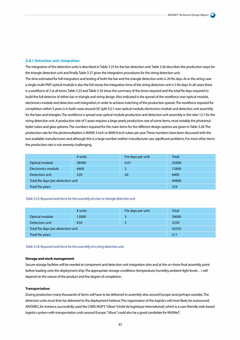
Optical module
Detection unit
Total fte days per detection unit
Total fte years
97
KM3NeT: Technical Design Report
3.6.1 Detection unit integration
The integration of the detection units is described in Table 3 25 for the bar detection unit. Table 3.26 describes the production steps for
the triangle detection unit and finally Table 3 27 gives the integration procedures for the string detection unit.
The time estimated for full integration and testing of both the bar and the triangle detection units is 20 fte days. As in the string case
a single multi-PMT optical module is also the full storey the integration time of the string detection unit is 5 fte days. In all cases there
is a workforce of 2 at all times. Table 3.23 and Table 3 24 show the summary of the times required and the total fte days required to
build the full detector of either bar or triangle and string design. Also indicated is the spread of the workforce over optical module,
electronics module and detection unit integration, in order to achieve matching of the production speeds. The workforce required for
completion within 5 years is in both cases around 50. Split 3:2:1 over optical module, electronics module and detection unit assembly
for the bars and triangles. The workforce is spread over optical module production and detection unit assembly in the ratio 12:1 for the
string detection unit. A production rate of 5 years requires a large yearly production rate of some items, most notably the photomul-
tiplier tubes and glass spheres. The numbers required for the main items for the different design options are given in Table 3.28. The
production rate for the photomultipliers is 80000 3 inch or 8000 8 inch tubes per year. These numbers have been discussed with the
two available manufacturers and although this is a large number neither manufacturer saw significant problems. For most other items
the production rate is not severely challenging.
Storage and stock management
Secure storage facilities will be needed at component and detection unit integration sites and at the on-shore final assembly point
before loading onto the deployment ship. The appropriate storage conditions (temperature, humidity, ambient light levels…) will
depend on the nature of the product and the degree of completion.
Transportation
During production many thousands of items will have to be delivered to assembly sites around Europe (and perhaps outside). The
detection units must then be delivered to the deployment harbour. The organisation of the logistics will most likely be outsourced.
ANTARES, for instance, successfully used the CNRS-IN2P3 ‘’Ulisse’’ (Unité de logistique international), which is a user-friendly web-based
logistics system with transportation units around Europe. ‘’Ulisse‘’ could also be a good candidate for KM3NeT.
Optical module
Electronics module
Detection unit
Total fte days per detection unit
Total fte years
Fte days per unit
0.67
2
20
# units
38400
6400
320
Total
25600
12800
6400
44800
224
Table 3.23: Required work force for the assembly of a bar or triangle detection unit.
Fte days per unit
3
5
# units
13000
650
Total
39000
3250
42250
211
Table 3.24: Required work force for the assembly of a string detection unit.


KM3NeT: Technical Design Report
104
Deployment of Junction Boxes
A design of the junction box has not been developed yet. For the deployment considerations we will assume that each junction box is
a structure with size 3 m x 3 m, a height of 2 m and a weight of no more than 3000 kg.
The deployment procedure is then analogous to the one described for the detection unit.
Connection of Detection Units and Junction Boxes
After the deployment of the telescope components an ROV will be used to connect them to the seabed network. The ROVs are
described in some detail in Section 3.7.2. The detection units and junction boxes are interconnected by a network of electro-optical
cables with lengths of the order of a few hundreds metres. These cables have to be accurately laid on the seafloor along well-deter-
mined paths in order to avoid damage to the network during successive deployment of telescope components and ROV operations.
Interlink cables that connect detection units to the secondary junction boxes will be deployed to the seabed together with the detec-
tion unit on drums. The drums are taken by the ROV and the cable unrolled on the seafloor. This method has been well tested in the
installation of ANTARES.
3.7.2 Vessels
The surface and deep-sea vessels needed are:
• a sea surface vessel, used to transfer, deploy and install components of the deep sea neutrino telescope at the bottom of the sea,
equipped with a Dynamic Positioning (DP) system;
• a deep-sea ROV.
Sea surface vessels
The sea surface vessel used in deploying the telescope components has to be equipped with a dynamic positioning system in order
to allow for accurate positioning of the detection units. For safety reasons a vessel equipped with a fully redundant dynamic position-
ing system would be advisable. In addition, the ship deck should have a size adequate for many detection units and be equipped with
lifting equipment.
The minimal characteristics of the sea surface vessels are:
• Dynamic positioning system able to maintain the ship position to within 1 m for sea states up to level 5;
• Available space on the ship deck of ~250 m2;
• Crane for 10 t load;
• A winch with a long cable, a cable speed control for between 0.1 m/s and 1 m/s, a load measuring system with 100 kg accuracy and
heave compensation;
• Ship deck allowing at least 1500 kg/m2 load;
• Extra space on the ship deck for two standard 20 foot equipment containers.
Two general variants of the deployment operations are being considered:
• A surface vessel equipped with a dynamic positioning system is used both for the transportation of the detection units from shore
and for the deployment operation. Such vessels can be contracted for defined periods of time and are permanently shuttling
between shore and site.
• An adequate vessel (e.g. a transport barge) is used for the transfer of the components to the site. A surface platform, equipped with a
dynamic positioning system and the other required equipment is used for the actual deployment. This deployment platform could
be an offshore supply vessel with an adequate deck space for storage of the detector parts to be deployed.


Recommended