ÉCOLE DE TECHNOLOGIE SUPÉRIEURE UNIVERSITÉ DU QUÉBEC
MANUSCRIPT-BASED THESIS PRESENTED TO ÉCOLE DE TECHNOLOGIE SUPÉRIEURE
IN PARTIAL FULFILLEMENT OF THE REQUIREMENTS FOR THE DEGREE OF DOCTOR OF PHILOSOPHY
Ph. D.
BY Hesam FARSAIE ALAIE
DIAGNOSIS OF DISEASES IN NEWBORN INFANTS BY ANALYSIS OF CRY SIGNALS
MONTREAL, JUNE 8th 2015
© Copyright Hesam FARSAIE ALAIE, 2015 All rights reserved

© Copyright
Reproduction, saving or sharing of the content of this document, in whole or in part, is prohibited. A reader
who wishes to print this document or save it on any medium must first obtain the author’s permission.
BOARD OF EXAMINERS (THESIS PH.D.)
THIS THESIS HAS BEEN EVALUATED
BY THE FOLLOWING BOARD OF EXAMINERS Prof. Chakib Tadj, Thesis Supervisor Department of Electrical Engineering at École de technologie supérieure Prof. Christian Gargour, Chair, Board of Examiners Department of Electrical Engineering at École de technologie supérieure Prof. Jérémie Voix, Member of the jury Department of Mechanical Engineering at École de technologie supérieure Prof. Patrick Kenny, External Evaluator Computer Research institute of Montréal
THIS THESIS WAS PRENSENTED AND DEFENDED
IN THE PRESENCE OF A BOARD OF EXAMINERS AND THE PUBLIC
MAY 8th 2015
AT ÉCOLE DE TECHNOLOGIE SUPÉRIEURE


ACKNOWLEDGMENTS
Thanks are in order for all the people who have helped me in realizing this doctorate thesis.
My heartfelt gratitude is in order for my director at École de Technologie Supérieure, Dr.
Chakib Tadj for his supervision and support. His invaluable support helped me to get into the
doctorate program and overcome all the difficulties through the period of my PhD study. He
let me find my own path whilst at the same time showing me which alternate paths I might be
missing and giving me advice in courses, in thesis writing, in securing grants, in dealing
language problems between English and French, in personal problem in my life.
I also would like to thank the jury members who evaluated my thesis and for their
constructive suggestions and helpful advice.
Apart from academic people mentioned above, I would also like to thank all my colleagues in
MMS laboratories for all the technical help and support during the period of my PhD study in
Montréal.
I would like to dedicate this thesis to my parents, Ahmad and Fatemeh, my brother Hossein
and thanks them for all the support, they provided for me during this stage of my life. This
was simply not possible without their encouragement and unconditional love. Thanks mom
and dad for all your love.
Finally, I acknowledge the financial support from Bill & Melinda Gates Foundation.


DIAGNOSIS OF DISEASE IN NEWBORN INFANTS BY ANALYSIS OF CRY SIGNALS
Hesam FARSAIE ALAIE
SUMMARY
Crying is the first sound the baby makes when he enters the world outside of his mother’s stomach, which is a very positive sign of a new healthy life. Well, we elders can talk but the newborn infant isn't old enough to do that yet. Cry is all a baby can do to express any discomfort it feels. When initially reading it, the first thing that comes to mind is why the cry is such an important aspect of health care for newborn infants? Although studying on infant’s cry was pioneered in the late 1960s, but it never crossed anybody's mind that sick infants might be identified from their cries. Statistical reports by World Health Organization state that the congenital anomalies or birth defects affect approximately 1 in 33 infants born every year and almost all of the world’s infant deaths happen in developing countries. Therefore, it is imperative to provide an inexpensive health care system, with no need of complex and advanced technology for poor mothers with newborn babies in low-income countries to survive more babies beyond the first months of life. In spite of the fact that there are a lot of maternal issues that can raise the risks of complications and anomalies in newborn infants, we are curious to examine the ability of solely the concealed information inside infant’s cry to clarify the infant’s physiological anatomy and psychological condition. The creative idea behind of such a non-invasive diagnostic system is based on the evidence extracted from past research studies for potential ability of infant’s cry to distinguish between healthy and sick infants. This innovative idea can tackle key global health and development problems. The purpose of this study is to develop a newborn cry-based diagnostic system to classify healthy and sick infants with different pathological conditions. First, an informed choice of pathological states and collecting of the infant cry data base is necessary and still in progress to complete the infant cry data base. In many of today’s application domains, it is often unavoidable to have data with high dimensionality and small sample size. Both small sample size problem and dimensionality reduction methods have been studied extensively but the combination of imbalanced data and small sample size presents a new challenge to the community. In this situation, learning algorithm often fail to generalize inductive rules over the sample space when presented with this form of imbalance. In fact, the combination of small sample size and high dimensionality hinders learning because of difficulty involved in forming conjugations over the high degree of features with limited samples. In the next part, data preprocessing, including selection and extraction of pathologically-informed features suitably with the best possible precision and then quantifying them for each pathological condition without any human intervention is considered in the system. In order to obtain the full benefit of the information embedded in the cry signal, Mel Frequency Cepstrum Coefficient (MFCC) analysis will be done on both expiratory and inspiratory cry vocalizations separately in this study. To avoid the need of human effort in labeling the boundaries of the corresponding corpus, automatic labeling of cry signals is required for an
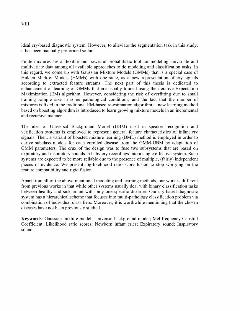
VIII
ideal cry-based diagnostic system. However, to alleviate the segmentation task in this study, it has been manually performed so far. Finite mixtures are a flexible and powerful probabilistic tool for modeling univariate and multivariate data among all available approaches to do modeling and classification tasks. In this regard, we come up with Gaussian Mixture Models (GMMs) that is a special case of Hidden Markov Models (HMMs) with one state, as a new representation of cry signals according to extracted feature streams. The next part of this thesis is dedicated to enhancement of learning of GMMs that are usually trained using the iterative Expectation Maximization (EM) algorithm. However, considering the risk of overfitting due to small training sample size in some pathological conditions, and the fact that the number of mixtures is fixed in the traditional EM-based re-estimation algorithm, a new learning method based on boosting algorithm is introduced to learn growing mixture models in an incremental and recursive manner. The idea of Universal Background Model (UBM) used in speaker recognition and verification systems is employed to represent general feature characteristics of infant cry signals. Then, a variant of boosted mixture learning (BML) method is employed in order to derive subclass models for each enrolled disease from the GMM-UBM by adaptation of GMM parameters. The crux of the design was to fuse two subsystems that are based on expiratory and inspiratory sounds in baby cry recordings into a single effective system. Such systems are expected to be more reliable due to the presence of multiple, (fairly) independent pieces of evidence. We present log-likelihood ratio score fusion to stop worrying on the feature compatibility and rigid fusion. Apart from all of the above-mentioned modeling and learning methods, our work is different from previous works in that while other systems usually deal with binary classification tasks between healthy and sick infant with only one specific disorder. Our cry-based diagnostic system has a hierarchical scheme that focuses into multi-pathology classification problem via combination of individual classifiers. Moreover, it is worthwhile mentioning that the chosen diseases have not been previously studied. Keywords: Gaussian mixture model; Universal background model; Mel-frequency Cepstral Coefficient; Likelihood ratio scores; Newborn infant cries; Expiratory sound; Inspiratory sound.

LE DIAGNOSTIC DES PATHOLOGIES CHEZ LES NOUVEAU-NÉS PAR L'ANALYSE DES SIGNAUX DE CRIS
Hesam FARSAIE ALAIE
RÉSUMÉ
Le cri est le premier son qu’un bébé peut générer à la naissance, et qui est également un signe positif d’une nouvelle vie saine. Ainsi, le cri est tout ce qu’un nourrisson peut faire pour exprimer un quelconque malaise qu’il ressent. Nous pouvons alors nous demander : pourquoi un cri est-il un aspect important des soins de santé dispensés aux nouveau-nés ? Bien que les études sur les cris des nouveau-nés aient été initiées depuis la fin des années 1960, peu de travaux ont été réalisés en vue de l’identification automatique de pathologies à partir du cri. Les rapports statistiques de l’Organisation mondiale de la santé indiquent que les anomalies congénitales ou malformations à la naissance affectent environ 1 nouveau-né sur 33 chaque année, et tous les décès d’enfants dans le monde ont majoritairement lieu dans les pays en développement. Il est donc impératif de fournir, aux pauvres mères dans les pays à bas revenu, un système économique de soins de santé qui aide leurs nouveau-nés à survivre au-delà des premiers mois de la vie, sans avoir à recourir à des technologies complexes et avancées. Malgré le fait qu’il y ait beaucoup de problèmes de santé maternelle qui peuvent augmenter les risques des complications et des anomalies chez les nouveau-nés, nous sommes avides de savoir à quel point l’information dissimulée dans le cri pourrait permettre l’identification de l’anatomie physiologique ainsi que de la condition psychologique chez un nouveau-né. L’idée créative d’un tel système non invasif de diagnostic est basée sur les données probantes ressorties des recherches antérieures qui à leur tour révèlent la possibilité de distinguer entre enfants malades et enfants sains à partir du cri. Cette idée innovatrice peut aborder les principaux enjeux en matière de santé et de développement. Le but de cette étude est de développer un système de diagnostic basé sur les cris afin de classifier les bébés sains et malades avec différents états pathologiques. D’abord, il est important de faire un choix précis des états pathologiques pour la phase de collection des cris des nouveau-nés. Cette opération est encore en cours pour compléter la base de données de cris. De plus, dans de nombreux domaines d’applications, il est souvent incontournable de disposer de données à très haute dimensionnalité et de taille d’échantillons réduite. Les problèmes de la taille des échantillons et de la réduction de la dimensionnalité ont fait l’objet des nombreuses recherches, mais l’association des données déséquilibrées et la taille réduite des échantillons réduite présente un nouveau défi pour la communauté. Dans cette situation, les algorithmes d’apprentissage échouent souvent à généraliser des règles inductives sur l’espace de l’échantillon et surtout lorsqu’ils sont employés avec cette forme de déséquilibre.
X
En effet, l’utilisation d’un échantillon, de taille réduite et de haute dimensionnalité, peut avoir un impact négatif sur l’apprentissage en raison de la difficulté dans la formation des relations par rapport au niveau déjà élevé des caractéristiques avec un nombre limité d’échantillons. Dans la partie qui suit, une étape de prétraitement des données, y compris la sélection et l’extraction des caractéristiques pathologiques appropriées avec la meilleure précision possible ainsi que leur quantification pour chaque pathologie, sans aucune intervention humaine, sera considérée pour l’élaboration de notre système. Afin d’exploiter l’information contenue dans le signal du cri, l’analyse des coefficients cepstraux sur l’échelle de Mels (MFCC) sera effectuée dans cette étude de façon séparée sur chacun des types de vocalisations expiratoire et inspiratoire du cri. En tenant compte de la nécessité d’éviter les efforts humains dans l’étiquetage des frontières dans le corpus utilisé, une étape de segmentation automatique des signaux de cris est requise pour un système de diagnostic idéal. Cependant, en vue d’alléger la tâche de segmentation dans cette étude, il était nécessaire jusqu’à présent de l’effectuer manuellement. Les mélanges finis sont des outils de modélisation probabilistes, flexibles et puissants parmi toutes les approches disponibles. Elles permettent la modélisation et la de classification de données univariables et multivariables. Nous avons ainsi choisi d’utiliser les modèles de mélanges gaussiennes (GMM), qui représentent un cas particulier des Modèles de Markov cachés (HMMs) avec un seul état, pour la représentation des signaux cris selon les vecteurs de caractéristiques extraites. La partie suivante de cette thèse est dédiée à l’amélioration de l’apprentissage des GMMs. Cette étape est généralement réalisée à l’aide d’un algorithme itératif EM, pour Expectation-Maximisation. Cependant, compte tenu, d’une part, du risque du sur-apprentissage (overfitting) en raison de la petite taille de des échantillons de certaines conditions pathologiques, et d’autre part, du fait que le nombre de mélanges est fixé dans l’algorithme de ré-estimation traditionnelle EM, une nouvelle méthode d’apprentissage fondée sur un algorithme de ‘boosting’ est introduite afin d’entrainer les modèles de mélanges croissantes d’une façon incrémentale et récursive. L’idée du modèle universel (UBM), largement employé dans les systèmes de reconnaissance du locuteur et de vérification, est utilisée pour représenter les caractéristiques principales des signaux de cris des nourrissons. Une variante de l’algorithme d’apprentissage appelée BML, pour Boosted Mixture Learning est employée, afin d’obtenir des modèles de chaque pathologie étudiée à partir d’un GMM-UBM par une adaptation des paramètres du GMM. L’essentiel dans la manipulation d’un système efficace de diagnostic est la fusion des deux sous-systèmes basés sur les vocalisations expiratoires et inspiratoires détectées dans les enregistrements des cris des bébés. De tels systèmes sont censés être plus fiables du fait de la présence de plusieurs éléments de preuve indépendants. En tenant compte de la compatibilité

XI
des caractéristiques et de la rigidité de la fusion, nous illustrons le rapport de fusion du Log-vraisemblance. Indépendamment de toutes les méthodes d’apprentissage et de modélisation susmentionnées, notre travail se différencie des travaux antérieurs par le fait que dans les autres systèmes, une tâche binaire de classification est utilisée et qui sert à distinguer entre bébés sains et bébés malades ayant seulement une pathologie spécifique. Alors que notre système de diagnostic est fondé sur un schéma hiérarchique qui se focalise sur le problème de classification multipathologies via la fusion de divers classificateurs individuels. Par ailleurs, il convient de souligner que les pathologies sélectionnées n’ont pas été étudiées auparavant. Mots clés: Modèles de mélanges gaussiennes ; Modèle universel (UBM) ; Coefficients Cepstraux; Rapport de vraisemblance ; cris des nouveau-nés ; Expiration ; Inspiration.


TABLE OF CONTENTS
Page
INTRODUCTION .....................................................................................................................1
CHAPITRE 1 REVIEW OF THE STATE OF THE ART ..................................................9 1.1 Fundamental concepts ....................................................................................................9
1.1.1 Definitions and elucidation ......................................................................... 9 1.1.2 Types of cries in infants ............................................................................ 14
1.2 Background ..................................................................................................................16 1.2.1 Mortality rate and birth defects ................................................................. 16 1.2.2 Primary research ....................................................................................... 20 1.2.3 Early-infant medical researches ................................................................ 24 1.2.4 Review of studies on machine learning and classification problems ....... 28
1.3 Cry pattern classification .............................................................................................35 1.3.1 Brief description on various classifiers ..................................................... 37
1.3.1.1 ANN and SVM .......................................................................... 37 1.3.1.2 Decision tree .............................................................................. 39 1.3.1.3 Naïve Bayes ............................................................................... 40 1.3.1.4 K-nearest neighbor ..................................................................... 41
1.3.2 Why Gaussian Mixture Models? .............................................................. 41 1.3.2.1 Introduction to GMMs ............................................................... 43 1.3.2.2 Learning of GMMs .................................................................... 44 1.3.2.3 Boosting algorithm..................................................................... 46
1.4 Brief objectives, methodologies and contributions ......................................................47 1.5 Summary ......................................................................................................................50
CHAPITRE 2 CRY-BASED CLASSIFICATION OF HEALTHY AND SICK INFANTS USING ADAPTED BOOSTED MIXTURE LEARNING METHOD FOR GAUSSIAN MIXTURE MODELS ................................53
2.1 Abstract ........................................................................................................................54 2.2 Introduction ..................................................................................................................54 2.3 GMMs for Cry-Pattern Classification ..........................................................................56 2.4 Newborn Cry-Based Diagnosis System (NCDS) ........................................................58
2.4.1 Cry Database ............................................................................................. 58 2.4.2 Pre-processing and feature extraction ....................................................... 58 2.4.3 Adapted BML method for GMMs ............................................................ 62 2.4.4 Initialization of sample weights ................................................................ 64 2.4.5 Process of adding a new component ......................................................... 65 2.4.6 Partial and global updating ....................................................................... 66 2.4.7 Criterion for model selection .................................................................... 67 2.4.8 Decision rule ............................................................................................. 68
2.5 Experiments .................................................................................................................69
XIV
2.6 Conclusion ...................................................................................................................76 2.7 Acknowledgment .........................................................................................................77
CHAPITRE 3 SPLITTING OF GAUSSIAN MODELS VIA ADAPTED BML METHOD PERTAINING TO CRY-BASED DIAGNOSTIC SYSTEM .79
3.1 Abstract ........................................................................................................................80 3.2 Introduction ..................................................................................................................80 3.3 Gaussian mixture model ..............................................................................................82 3.4 Adapted boosted mixture model ..................................................................................83
3.4.1 Process of adding a new component ......................................................... 84 3.4.2 Partial and global updating ....................................................................... 85 3.4.3 Initialization of sample weights ................................................................ 86 3.4.4 Criterion for model selection .................................................................... 87
3.5 Experiments .................................................................................................................89 3.5.1 Preprocessing and feature extraction ........................................................ 89 3.5.2 Multi-pathology classification .................................................................. 90
3.6 Conclusion ...................................................................................................................92 3.7 Acknowledgment .........................................................................................................93
CHAPITRE 4 CRY-BASED INFANT PATHOLOGY CLASSIFICATION USING GMMS .......................................................................................................95
4.1 Abstract ........................................................................................................................96 4.2 Introduction ..................................................................................................................97
4.2.1 Early studies and birth defects .................................................................. 97 4.2.2 Related studies ........................................................................................ 100
4.3 Recording procedure and cry data base .....................................................................101 4.4 Feature extraction.......................................................................................................103
4.4.1 Preprocessing stages ............................................................................... 104 4.4.2 Static and dynamic MFCCs .................................................................... 105
4.5 Statistical modeling and descriptions .........................................................................108 4.5.1 Likelihood ratio detector ......................................................................... 109 4.5.2 Gaussian mixture models ........................................................................ 111 4.5.3 System description .................................................................................. 112 4.5.4 Applying the GMM-UBM ...................................................................... 114 4.5.5 BML adaptation of sub-models or health-dependent-infant cry model .. 116
4.6 Evaluations and experiments .....................................................................................119 4.6.1 Defining GMM-UBM and adaptation methods ...................................... 119 4.6.2 Log-likelihood score computation .......................................................... 120 4.6.3 Health-condition detection system .......................................................... 123
4.6.3.1 Healthy infant detector ............................................................. 123 4.6.3.2 Sick infant detector with a specific disease ............................. 129
4.6.4 Fusion, calibration and decision ............................................................. 131 4.6.5 Results and discussion ............................................................................ 133
4.7 Conclusion and further discussion .............................................................................145 4.8 Acknowledgment .......................................................................................................148

XV
CONCLUSION 149
RECOMENDATIONS ..........................................................................................................155


LIST OF TABLES
Page
Table 1.1 Comparison of the first three cry signals after pain stimulus ....................15
Table 1.2 Deaths and percentage of total deaths for the 11 leading causes of infant death: United States, 2010 ...............................................................17
Table 1.3 Maternal age versus risk of DS ..................................................................17
Table 1.4 Similarities between hunger, first birth, and pleasure cry .........................21
Table 1.5 Comparison table between cry characteristics of several diseases ............22
Table 1.6 Comparison table between cry characteristics of healthy and sick infants .................................................................................................23
Table 1.7 Confusion matrix .......................................................................................24
Table 1.8 Cry features of infants with severe pathologies .........................................25
Table 1.9 Cry features of infants with undetectable disease with not clear prognosis ...........................................................................................27
Table 1.10 Confusion matrix of Neural Network with SCG algorithm .......................30
Table 1.11 The winning combination with 10 features ...............................................31
Table 1.12 Confusion matrix of RBF network ............................................................31
Table 1.13 Determination of FN1 ................................................................................32
Table 1.14 Determination of decision parameter .........................................................33
Table 1.15 Confusion matrix of the ensemble method ................................................33
Table 1.16 Comparison accuracies of FFNN with PCA and statistic reduction ..........34
Table 1.17 Comparison table between best results of classifiers and their ensembles ...........................................................................................34
Table 1.18 Obtained accuracy rate in each decomposition level for PNN classification .....................................................................................36
Table 2.1 Cry database ...............................................................................................59

XVIII
Table 2.2 Obtained accuracy rate for multi-pathology classification (%) .................71
Table 2.3 Confusion Matrix for defined Binary classification task ...........................75
Table 2.4 Obtained two statistical measures for Binary-classification problem ........76
Table 3.1 Cry database ...............................................................................................90
Table 3.2 Obtained accuracy rate (%) for multi-pathology classification task ..........92
Table 4.1 Different units available in the CDB .......................................................102
Table 4.2 List of health-conditions ..........................................................................103
Table 4.3 Number and duration of the recorded cry signals that were available in the training CDB at the time .................................................117
Table 4.4 Number of infants and recorded cry signals available in the testing CDB at the time ............................................................................122
Table 4.5 Number of cry samples that contain EXP/INSV-labeled segments and 3-sec cry units in our test CDB .........................................................122
Table 4.6 Comparison of the different healthy infant detector systems based on the Equal error rate and Area under the curve for all of the test samples ..............................................................................................128
Table 4.7 Comparison of the different healthy infant detector systems based on the EER and AUC for the test samples that have more than 3 INSV units (32 and 23 cry samples of healthy and sick infants respectively) .............................................................................................128
Table 4.8 Results of the sick infant detector systems for Respiratory and Neurological disorders .............................................................................130
Table 4.9 Training parameters used in SVM, PNN and MLP .................................132
Table 4.10 Number of folds and rounds ....................................................................133
Table 4.11 Average accuracy, sensitivity and specificity over the used classifiers in the healthy infant detection task .........................................137
Table 4.12 Accuracy rates for the used classifiers in the healthy infant detection task ...........................................................................................138
Table 4.13 Sensitivity rates for the used classifiers in the healthy infant detection task ...........................................................................................139

XIX
Table 4.14 Specificity rates for the used classifiers in the healthy infant detection task ...........................................................................................139
Table 4.15 Average accuracy, sensitivity and specificity over the used classifiers in the sick infant (affected by neurological problems) detection task ...........................................................................................143
Table 4.16 Average accuracy, sensitivity and specificity over the used classifiers in the sick infant (affected by respiratory disorders) detection task ...........................................................................................144

LIST OF FIGURES
Page
Figure 1.0 The desired system .....................................................................................14
Figure 1.1 Rhythmic pattern of a typical infant cry ....................................................14
Figure 1.2 Pattern of Pain Cry .....................................................................................15
Figure 1.3 Infant mortality by gestational age in the U.S. in 2010 .............................18
Figure 1.4 Relation of weight and gestational age for (a) male and (b) female singletons ...................................................................................................19
Figure 1.5 Median values, the 25th and 75th percentiles of the ....................................28
Figure 1.6 Block diagram of auto diagnostic system by using pattern recognition ....28
Figure 1.7 Linear prediction analysis on 1 second of cry signal .................................29
Figure 1.8 Structure of a basic RBF network ..............................................................30
Figure 1.9 Obtained densities for uni-modal Gaussian model, GMM, and VQ ..........42
Figure 1.10 The general system diagram ......................................................................48
Figure 1.11 The growing process of finite mixture model ............................................49
Figure 1.12 Modeling and decision ...............................................................................50
Figure 2.1 Time domain representation of a cry signal ...............................................59
Figure 2.2 Pre-processing steps ...................................................................................62
Figure 2.3 Block diagram of learning GMM using .....................................................68
Figure 2.4 Mapping of estimated GMMs to pathological conditions .........................69
Figure 2.5 Mean classification accuracy rates .............................................................72
Figure 2.6 Coefficient of variation ..............................................................................73
Figure 2.7 Number of components ..............................................................................74
Figure 3.1 Block diagram of adapted BML technique ................................................88

XXII
Figure 3.2 Estimated contour (a) of the first Gaussian component, (b) after splitting GMM into 2 components, (c) of final GMM ...............................89
Figure 4.1 Leading causes of infant deaths in 193 countries in 2010 .........................98
Figure 4.2 Cumulative power spectrum of (a-c) EXP units, (b-d) INSV units for each health condition .................................................................106
Figure 4.3 Pre-processing and MFCC feature extraction steps .................................107
Figure 4.4 Balanced data pooling approaches for two defined GMM-UBM ............115
Figure 4.5 Mean of the LLR scores over INSV cry units inside the (a) healthy and (b) sick infants for the healthy infant verification system .................121
Figure 4.6 DET curves for two alternative hypothesized models λPI − UBM (a-c) and λHyp (b-d) and for INSV (a-b) and EXP (c-d) cry units with a 10 ms frame length in the healthy infant verification system .......124
Figure 4.7 DET curves for two alternative hypothesized models λPI − UBM (a-c) and λHyp (b-d) and for INSV (a-b) and EXP (c-d) cry units with the 30 msec frame length in the healthy infant verification system ........125
Figure 4.8 Type I and type II errors of the tested different healthy infant detector systems for each of the adaptation methods ............................................136
Figure 4.9 Type I and type II errors for the SVM with different kernel functions in the healthy infant detection task ..........................................................137
Figure 4.10 Comparison of the accuracy rates of all of the classifiers in the healthy infant detection task ....................................................................138
Figure 4.11 Type I and type II errors of the classifiers used in the healthy infant detection task using 400 repeated 3-fold CVs for the test samples that contain more than 3 EXP and INSV-labeled cry units ............................140
Figure 4.12 Type I and type II errors for the different classifiers in the sick infant (affected by neurological problems) detection task .................................142
Figure 4.13 Comparison of the accuracy rates of all of the classifiers in the sick infant (affected by neurological problems) detection task .......................142
Figure 4.14 Type I and type II errors for the different classifiers in the sick infant (affected by respiratory disorders) detection task ....................................144
Figure 4.15 Comparison of the accuracy rates of all of the classifiers in the sick infant (affected by respiratory disorders) detection task ..........................145

XXIII
Figure 4.16 Introduced system overview ....................................................................152

LIST OF ABREVIATIONS, INITIALS AND ACRONYMS AGA Appropriate for gestational age
AIC Akaike information criterion
ANN Artificial neural network
ANOVA Analysis of variance
ASR Automatic speech recognition
AUC Area under cover
BIC Bayesian information criterion
BML Boosted mixture learning
CDB Cry data base
CDC Center for disease control
CE Cross entropy
CNS Central nervous system
CV Coefficient of variation
DCT Discrete cosine transform
DET Detection error tradeoff
DS Down syndrome
DWT Discrete wavelet transform
EER Equal error rate
EM Expectation maximization
EXP Expiration
FAR False acceptance rate
FFNN Feed-forward neural network
FFT Fast Fourier transform
FIR MLP Finite impulse response multilayer response
FN False negative
FP False positive
FRR False rejection rate
GMM Gaussian mixture model
GMM-ML Gaussian mixture model-maximum likelihood
XXVI
GFCC Gamma-tone frequency Cepstral coefficients
GRNN General regression neural network
GSFM Genetic Selection of a Fuzzy Model
HMM Hidden Markov model
HPF High Pass Filter
HTK Hidden Markov model toolkit
INSV Inspiration voiced
KNN K-nearest neighbor
LBW Low birth weight
LGA Large for gestational age
LLR Log-likelihood ratio
LP Linear prediction
LPC Linear prediction coefficients
LVQ Linear vector quantization
MAP Maximum a posteriori
MFCC Mel frequency Cepstral coefficients
MFDWC Mel frequency discreet wavelet coefficients
ML Maximum likelihood
MLP Multilayer perceptron
MMI Maximum mutual information
ms Millisecond
NCDS Newborn cry-based diagnosis system
NICU Neonatal intensive care unit
NIST National institute of standard and technology
OP Operation point
PCA Principle component analysis
PNN Probabilistic neural network
PSD Power spectral density
RBF Radial basis function
RDS Respiratory distress syndrome
XXVII
ROC Receiver operating characteristic
SCG Scaled conjugate gradient
SFFS Sequential forward floating search
SGA Small for gestational age
SIDS Sudden infant death syndrome
SMO Sequential minimal optimization
SRE Speaker recognition evaluation
SVM Support vector machine
TDNN Time delay neural network
TN True negative
TP True positive
UBM Universal background model
VAD Voice activation detection
VQ Vector quantization
WHO World health organization
WPT Wavelet packet transform
WTCC Wavelet transform-based Cepstral coefficient

INTRODUCTION
Context of Research Work
Crying is the first and clear sign of life which is seen clearly shortly after the baby’s live
birth. Reasons of infant’s cry are the same reason of speech in adult i.e. to let others know
about their needs or problems. In other words, every baby is born with the ability to express
their needs through sound. Therefore this multimodal signal carries a lot of information about
the baby. For example, Mrs. Priscilla Dunstan1 has decoded five universal infant cry patterns
as an easiest way to settle an inconsolable baby who can make a parent feel quite helpless
and powerless. These patterns are sort of a baby language based on phonetic sounds, which
are created as part of the automatic reflexes that all newborn babies make.
Analysis of infant cry signals was pioneered in the late 1960s in Scandinavia. After some
sound spectrographic cry analysis of infants with various diseases, in some cases it has been
noticed that there are fixed cry attributes, which are rarely seen in cries of healthy infants.
Instead, these attributes occur very often in cries of infants with diseases. Therefore it was
found that concealed information contained in infant cry signal can reflect a diverse range of
diseases and conditions that could affect an infant’s health. In early studies of infant cry, the
acoustic structure of infant crying was analyzed and some of the important variables
controlling the production of their cries were described. Afterwards, focus of attention was
shifted into the sounds produced by the hungry, lonely, pain, hurt, or generally discomforted
infants. Although there have been some books and products created through the years to
unlock the secret language of babies, their potential for use in the early diagnosis and
treatments in newborns remains largely in an open and undeveloped state.
1 http://www.dunstanbaby.com/
2
Statement of research problem
In recent years, there has been an increasing interest in cry analysis of sick newborn infants.
Due to high rate of mortality rate (about 2.7 million infants) in 193 countries in 2010
(Congenital anomalies, 2014), researchers have begun to take an interest in newborn infants
with congenital anomalies or babies who are preterm or at risk with infected Central Nervous
System (CNS). Moreover, the sudden death of an infant may occurs in some cases which is
not predictable by medical history and remains unexplained after detailed death scene
investigation, but some of them are actually result of accidents, abuse, and previously
undiagnosed conditions, such as metabolic disorders.
Recently, there has been a lot of interest in diagnosis tools that are affordable, easy-to-use
and can rapidly diagnose disease at the point of care and thereby reduce death, disability in
resource-poor communities. One of many bold ideas attracting investment from the Gates
Foundation’s Grand Challenges Explorations initiative to address global health and
development challenges is to provide special care and treatment that can prevent disability
and death early in life in resource-poor communities. Since approximately 1 percent of the
world’s infant deaths occur in developed countries based on the fact sheet2, the situation is
worse for many developing countries. Consequently, identifying illness in newborns from
their cries via a robust, inexpensive, and simple to use in point-of-care settings have the
ability to greatly improve the quality and efficacy of healthcare available to newborns in
developing countries, where the burden of disease is highest.
It never crossed anybody's mind a few years ago that sick infants might be identified from
their cries. However, based on current evidence for potential ability of infant’s cry to
distinguish healthy infant from those with medical problems, there is a good chance to be
2 The World factbook (Fact sheet No 348-Updated May 2104) Available in: http://www.who.int/mediacentre/factsheets/fs348/en/

3
successful in finding such a Newborn Cry-based Diagnosis System (NCDS). This innovative
idea can tackle key global health and development problems.
In this work, we focus on the means of the discriminative learning of GMM to suit the given
cry samples consisting of healthy and sick newborn infants with different pathological
conditions. A novel idea is used to adapt the parameters of the corresponding GMM-UBM to
derive either healthy or pathology subclass models separately. It is the principal contribution
that we offer in this research domain where lots of interests were expended for the
classification of cries of infants in pathological conditions.
Objective and methodology
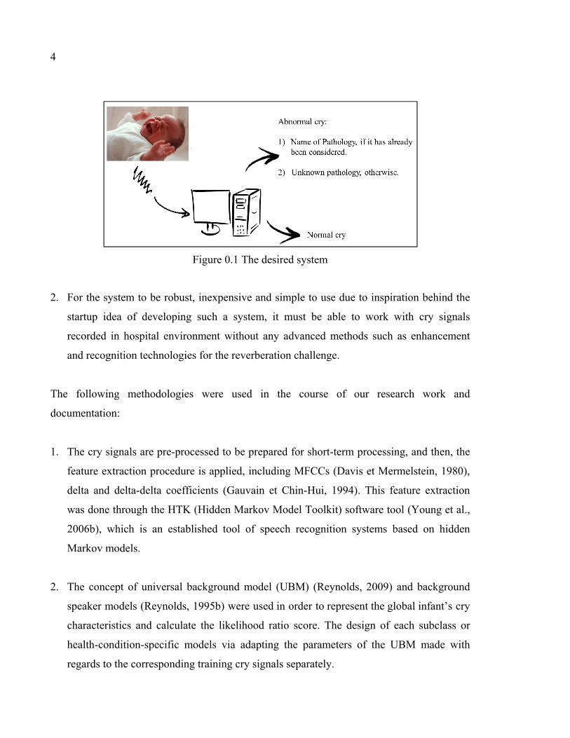
Our objective is to develop classification system to determine prognosis for newborn infants
with congenital diseases. The system creates a GMM-based pattern for either the expiratory
or inspiratory sounds of cry signals. It provides score level fusion of aforementioned models
in order to offer improvement in diagnostic and prognostic accuracy. Indeed, our objective is
to provide a cry-based classification system that is capable of modeling the acoustic
differences between wide range of developmental and pathological conditions affecting both
vulnerable preterm and full-term neonatal population. Once developed, the system is simple
to use: a recorder of the voice connected to a computer takes samples of the cry of the infant.
The result will be available after finishing data processing and cry classification process
instantly. Figure 0.1 shows various test results which will be provided by the system.
In order to attain this objective, the following approaches were conceived:
1. The paradigm that is to be developed should be generic in concept in order that the
proposed solution can be applied to any kind of infant disease with no or very little
adjustments.
4
Figure 0.1 The desired system
2. For the system to be robust, inexpensive and simple to use due to inspiration behind the
startup idea of developing such a system, it must be able to work with cry signals
recorded in hospital environment without any advanced methods such as enhancement
and recognition technologies for the reverberation challenge.
The following methodologies were used in the course of our research work and
documentation:
1. The cry signals are pre-processed to be prepared for short-term processing, and then, the
feature extraction procedure is applied, including MFCCs (Davis et Mermelstein, 1980),
delta and delta-delta coefficients (Gauvain et Chin-Hui, 1994). This feature extraction
was done through the HTK (Hidden Markov Model Toolkit) software tool (Young et al.,
2006b), which is an established tool of speech recognition systems based on hidden
Markov models.
2. The concept of universal background model (UBM) (Reynolds, 2009) and background
speaker models (Reynolds, 1995b) were used in order to represent the global infant’s cry
characteristics and calculate the likelihood ratio score. The design of each subclass or
health-condition-specific models via adapting the parameters of the UBM made with
regards to the corresponding training cry signals separately.

5
3. The traditional EM-based re-estimation (Dempster, Laird et Rubin, 1977) and maximum
a-posteriori (MAP) approach (Gauvain et Chin-Hui, 1994; Reynolds, Quatieri et Dunn,
2000) were employed to train GMMs and adapt the GMM-UBM respectively as a
reference system.
4. The concept of Log-likelihood ratio (LLR) (Reynolds, Quatieri et Dunn, 2000) was used
for a test sequence of feature vector. Both fast scoring method and score normalization
for a sequence of feature vector (Reynolds, Quatieri et Dunn, 2000) were employed to
reduce the computational complexity.
5. Mathematical equations were formulated to allow the reader a better understanding of
various concepts and idea within this thesis.
Organization of the thesis
The organization of this thesis is as follows:
The first chapter is a review of the past research studies whose goal is to illustrate their
contributions with regards to our work as well as to differentiate ours with them, therefore
illustrating our contributions to the domain. The three chapters that follow are published
works.
The second chapter is an article that was published in the Journal of Modeling and
Simulation in Engineering:
• Farsaie Alaie, Hesam, et Chakib Tadj. 2012. « Cry-Based Classification of Healthy and
Sick Infants Using Adapted Boosted Mixture Learning Method for Gaussian Mixture
Models ». Modeling and Simulation in Engineering, vol. 2012, p. 10.
In this article, we presented the major drawback of the conventional EM-based re-estimation
algorithm in designing and training the parameters of GMMs. We presented our preliminary
6
solution as an adapted boosted mixture learning method to train mixture models in an
incremental and recursive manner. We presented GMM as an effective probabilistic model
for our cry-based classification system. We also demonstrated that the performance of the
healthy infant classifier gradually improve when the frame duration for short-time processing
decrease from 30 to 20 msec.
The third chapter is an article that was published in the Journal of Engineering in 2013:
• Farsaie Alaie, Hesam, et Chakib Tadj. 2013. « Splitting of Gaussian Models via Adapted
BML Method Pertaining to Cry-Based Diagnostic System ». Engineering, vol. 5, p. 277-
283.
In this article, we introduced a discriminative splitting idea for GMMs followed by learning
via Adapted boosted mixture learning method. We also demonstrate that this method can stop
splitting process to find the minimum number of Gaussian components by maximizing the
objective function in each iteration and BIC. We employed this method to classify healthy
and sick infants including both full-term and premature based on ML decision criterion.
The fourth chapter is an article that was submitted in the Journal of Speech Communication
in January 2015:
• Farsaie Alaie, Hesam, Lina Abou-Abbas, Chakib Tadj. Jan 2015. « Cry-Based Infant
Pathology Classification Using GMMs ». Journal of Speech Communication.
In this article, we presented a hierarchical scheme that is a treelike combination of individual
detection system to identify healthy and sick infants at risk with neurological and respiratory
disorders. Each hypothesized health-condition class is derived from the corresponding UBM
by adapted BML procedure. We also demonstrated that due to small number of hypothesized
classes using the idea of background speaker models is practical in calculating the likelihood
ratio score and has better accuracy compared to UBM. Although it was shown that the

7
expiration cry sounds have better performance in the classification tasks, the system also
adapts a score level fusion of the expiratory and inspiratory sounds-based subsystems to
make a more reliable decision.
Finally, the last chapter is dedicated to conclusion of this thesis document as well as some
further research recommendations.

CHAPITRE 1
REVIEW OF THE STATE OF THE ART
In this chapter, we present the previous research studies that were related to ours. Many
authors have contributed to the development of such this classification system for different
types of diseases. A comparison between pattern recognition techniques helped us to better
understand what kind of features and classifier could be the best choice for our purpose.
Consequently, this chapter tries to emphasize the key role of both feature selection and
classification approach in such a system. Whenever there is a need to diffuse confusion, we
will define the terminologies used in this research to diminish ambiguity that may arise in the
discussion.
1.1 Fundamental concepts
This section has a primary concept of cry analysis and gives you a good view of cry signals
and their features. This information is not essential to follow the remainder of this thesis but
it may help you better understand where they came from and its importance.
1.1.1 Definitions and elucidation
In adult human speech communication, we use and interpret some of features unconsciously
and without really thinking. These so-called prosodic features go beyond phonemes and deal
with auditory qualities of sound. They convey attitudes, and emotional states which make
human speech sound human. The infant cry signals are all prosody. Thus, the infants express
their feeling, and their needs through acoustic correlates of the prosodic features such as
pitch, loudness, melody, and intonation. Lester et al in (Benson et Haith, 2009) defined three
identifiable cry modes of vocal fold vibration: basic-cry or phonation, high-pitch cry or
hyperphonation, noisy or turbulent cry or dysphonation. Most infants have a fundamental
frequency or pitch around 250-450 Hz. In phonation and hyperphonation modes only the
10
first two formants are usually measured and F1 occurs at approximately 1100 Hz and F2 at
approximately 3300 Hz.
Here are some terminologies and definitions of popular cry characteristics used in literature
on cry analysis (Benson et Haith, 2009; Lederman, 2002; Verduzco-Mendoza et al., 2009;
Wasz-Hockert, Michelsson et Lind, 1985).
Prosody: It is the intonation and melody patterns of an utterance.
Cry modes: It is a function of vibrational mode of vocal folds. Specific cry modes include:
Phonation, Hyperphonation, Dysphonation and Inspiratory Phonation.
Phonation: Category of cry sounds resulting from harmonic vibration (usually between 350
and 750 vibrations per second) of the vocal chords during an expiratory utterance.
Hyperphonation: Category of cry sounds caused by a change in vocal register resulting in a
harmonic vibration (usually between 1000 and 2000 vibrations per second) of the vocal
chords during an expiratory utterance.
Dysphonation: Category of cry sounds caused by a change in vocal register resulting in an
inharmonic or noisy.
Inspiratory phonation: Category of cry sounds resulting from vibration of the vocal folds
during an inspiratory utterance during an expiratory utterance.
Cry mode change: The number of times the cry modes change within any given utterance.
Fundamental frequency: Base frequency, during harmonic vibration (that includes the Cry
Modes of Phonation and Hyperphonation) of vocal cord vibration Fundamental Frequency is
usually heard as the pitch of the cry.

11
Formant frequencies ( . . . ): They are center frequencies of the theoretically infinite
number of resonances of the vocal tract system. The center frequency of the first resonance is
defined as the first formant (F ), and the second is defined as the second formant (F ), etc.
Only the first two or three formants are usually measured.
Maximum pitch: It is the highest measurable point of the fundamental frequency (f ).
Minimum pitch: It is a frequency after a rapid increase in the f contour.
Pitch of Shift (shift): It is a frequency after a rapid increase in the f contour.
Break: It is defined like the time interval between the end of a phonation and the next
inspiration.
Cry latency: It is the time between the pain stimulus and the onset of the first expiratory
utterance.
Voicedness: Voicedness is defined as being the ratio of the amount of periodic sound versus
the amount of noise.
Stridor: When the voicedness suddenly drops within an area of high energy, one occurrence
of stridor is marked. Tangibly, the following thresholds were selected: when the voicedness
drops to less than 30% of its maximum while the energy level remains above -35dB, one
occurrence of stridor is marked.
Melody type: Fundamental frequency variations that is either falling, rising-falling, rising,
falling rising, or fiat.
Noise concentration: High-energy peak at 2000 to 2300 Hz, found both in voiced and
voiceless signals. This attribute is clearly audible.

12
Bi-Phonation: It is an apparent double series of harmonics of two fundamental frequencies.
Unlike double harmonic break, these two series seem to be independent of each other.
Gliding: A very rapid up or down movement of f .
Continuity: A measure of whether the cry was entirely voiced, partly voiced, or voiceless.
Glottal stops: Short, expiratory bursts of sound created by a sudden opening and sustained
closing of the vocal folds.
Vibrato: It is at least four rapid up-and-down movements of f within one expiratory
utterance.
Voice-UnVoiced: The cries are voiced or unvoiced (voiceless). In the voiced cry the sound
wave is periodic and both fundamental and its harmonics are visible on the spectrogram. In
the inaudible unvoiced cries the spectrogram shows a burr turbulence or aperiodic noise with
a fundamental which is not visible, nor measurable.
The following is a brief definition of some diseases and disorders that are common among
newborn infants and used in related works and ours (Miller et O'Toole, 2003).
Down's Syndrome (trisomy 21): Down syndrome (DS) is the most common cause of mental
retardation and malformation in a newborn. It occurs because of the presence of an extra
chromosome.
Cri-du-chat: A hereditary congenital syndrome characterized by hypertelorism,
microcephaly, severe mental deficiency, and a plaintive catlike cry, due to deletion of the
short arm of chromosome 5.

13
Trisomy 13: A syndrome characterized by mental retardation and defects to the central
nervous system and heart, caused by having three copies of chromosome 13.
Trisomy 18: A congenital condition caused by the presence of an extra chromosome 18,
characterized by severe mental retardation and multiple deformities.
SIDS: It is a sudden and unexpected death of an apparently healthy infant, not explained by
careful postmortem studies. It typically occurs between birth and age 9 months, with the
highest incidence at 3 to 5 months.
Sepsis: It is a potentially deadly medical condition that is characterized by a whole-
body inflammatory state (called asystemic inflammatory response syndrome or SIRS) and
the presence of a known or suspected infection. In neonates, sepsis is difficult to diagnose
clinically. It is found in infants during the first month of life.
Bovine protein allergy: Cow's milk allergy is the most common food allergy in young
children. Bovine protein allergy constitutes an important place in childhood food allergies.
Soy protein-based and hydrolyzed protein formulas have some disadvantages.
Pre term infants: Babies who are born before 37 weeks, and particularly those born before
34 weeks, are at greater risk of suffering problems at birth.
Thrombosis in the vena cava: Renal venous thrombosis occurring in the neonate causes
haematuria, oliguria, acute renal failure, and hypertension.
Hypoxia: It is a deficiency in the amount of oxygen reaching body tissues.
Tetralogy of Fallot: It is a type of congenital land cyanotic heart defect. It causes low
oxygen levels in blood. This leads to cyanosis (a bluish-purple color to the skin).

14
Coarctation of Aorta: It is a narrowing of part of the aorta (the major artery leading out of
the heart). It is a type of birth defect. Aortic coarctation is more common in persons with
certain genetic disorders, such as Turner syndrome. However, it can also be due to birth
defects of the aortic valves.
1.1.2 Types of cries in infants
In relevant prior works, different kind of cry signals as a database is observed such as hunger
cry, pain cry, and normal cry. Crying due to pass 3 to 3.5 hours after last feeding of infants
has been referred as the hunger cry (Newman, 1985). Some studies have elicited pain cry
based on use of a stimuli such as rubber band snap, heel stick with a blood lancet, skin pinch
on the arm or ear, or removal of electrodes from infant’s body (Cacace et al., 1995). The
pleasure cry is produced by an infant who has been fed and changed and who shows clear
indications of being comfortable (Sagi, 1981).
Crying rate varies from 50 to 70 utterances per minutes, and duration of the each cry unit
ranges from 0.4 to 0.9 seconds. Figure 1.1 depicts a typical cry sequence which follows a
rhythmic pattern that is noticed 30 minutes after birth. The normal cry starts with a cry
coupled with a briefer silence, which is followed by a short high-pitched inspiratory whistle.
Next, there is a brief silence followed by another cry. Hunger is a main stimulant of the basic
cry. Greater variability in some cry parameters appears after the end of the second month.
Crying may continue in this manner during a period of 40 seconds to more than 4 minutes
(Newman, 1985).
Figure 1.1 Rhythmic pattern of a typical infant cry

15
Crying following a painful experience is called “Pain Cry” and a typical example of such
cry has a length of approximately 3 seconds. The pattern of such a cry is shown in Figure
1.2.
Figure 1.2 Pattern of Pain Cry
Although among the first three cry signals after the pain stimulus there were no marked
differences in cry characteristics (see Table 1.1), study on infants’ cries during the first six
months had shown few changes in the cry characteristics (Wasz-Hockert, Michelsson et
Lind, 1985).
Table 1.1 Comparison of the first three cry signals after pain stimulus
Max/Min pitch Shift Duration Glottal roll
1st Cry signal like the other
ones
more often longer and often
interrupted
more common
2nd Cry Signal like the other
ones
- shorter and often
continuous
-
3th Cry Signal like the other
ones
- shorter and often
continuous
-
Investigators studying cry characteristics have found diagnostic value in pain cry analysis.
For example, compared to normal infants’ cry, pain cries of infants with Down’s syndrome
are lower in pitch, longer, and flatter in melody contour (Wasz-Hockert et al., 1968).
16
1.2 Background
This section briefly presents some birth prevalence rates of selected birth defects and causes
of infant death. Moreover, some previous research studies that are related to ours are
reviewed.
1.2.1 Mortality rate and birth defects
Statistics reports by World Health Organization (Congenital anomalies, 2014) and Center for
Disease Control and prevention (Rynn, 2008) present that the congenital anomalies or birth
defects affect about 1 in 33 born infants every year. In an article published by the New
Brunswick Beacon (Silverthorne, 2014), it was reported that according to press released from
the CDC and the Public Health Agency of Canada, the risk of birth defects in Canadian
babies is higher than American. Moreover, based on the Factbook published by Central
Intelligence Agency (The World factbook, 2013-14), United States’ infant mortality rate is
6.17 per 1,000 live birth which is higher than at Canada of 4.71 rate. In Table 1.2 the leading
causes of infant death in the U.S. in 2010 are listed (Heron, 2013).
Heart defect, neural tube defects and Down syndrome are especially prevalent among
infants (Congenital anomalies, 2014). Down syndrome, also known as trisomy 21, is a
genetic disorder which is fairly common chromosomal abnormality among infants (about
1 in 800 (Lobo et Zhaurova, 2008)). This genetic disorder can often infect other parts of
the body and bring on other diseases such as heart defects, leukemia and Alzheimer’s
disease. There are a lot of maternal and environmental issues which can raise the risks of
several complications and associated anomalies, such as gestational age, birth weight,
consanguinity (relationship by blood), maternal age, multiple gestations, and maternal
infection during pregnancy, socioeconomic factors and maternal nutritional status. For
example, the risk of having a baby with DS (Lobo et Zhaurova, 2008) increases as she
gets older (see Table 1.3).

17
Table 1.2 Deaths and percentage of total deaths for the 11 leading causes of infant death: United States, 2010
Adapted from Heron (2013)
Cause of death Rank Deaths Percent of
total deaths
All causes … 24,586 100.0
Congenital malformations, deformations
and chromosomal abnormalities
1 5,107 20.8
Disorders related to short gestation and low
birth weight, not elsewhere classified
2 4,148 16.9
Sudden infant death syndrome 3 2,063 8.4
Newborn affected by maternal
complications of pregnancy
4 1,561 6.3
Accidents (unintentional injuries) 5 1,110 4.5
Newborn affected by complications of
placenta, cord and membranes
6 1,030 4.2
Bacterial sepsis of newborn 7 583 2.4
Respiratory distress of newborn 8 514 2.1
Diseases of the circulatory system 9 507 2.1
Neonatal hemorrhage 11 458 1.8
Necrotizing enter colitis of newborn 10 472 1.9
Table 1.3 Maternal age versus risk of DS Adapted from Lobo (2008)
Age Risk
Age < 35 0.05 % (or 1 in 2,000)
Age 40 1 % (or 1 in 100)
Age 50 8.3 % (or 1 in 12)
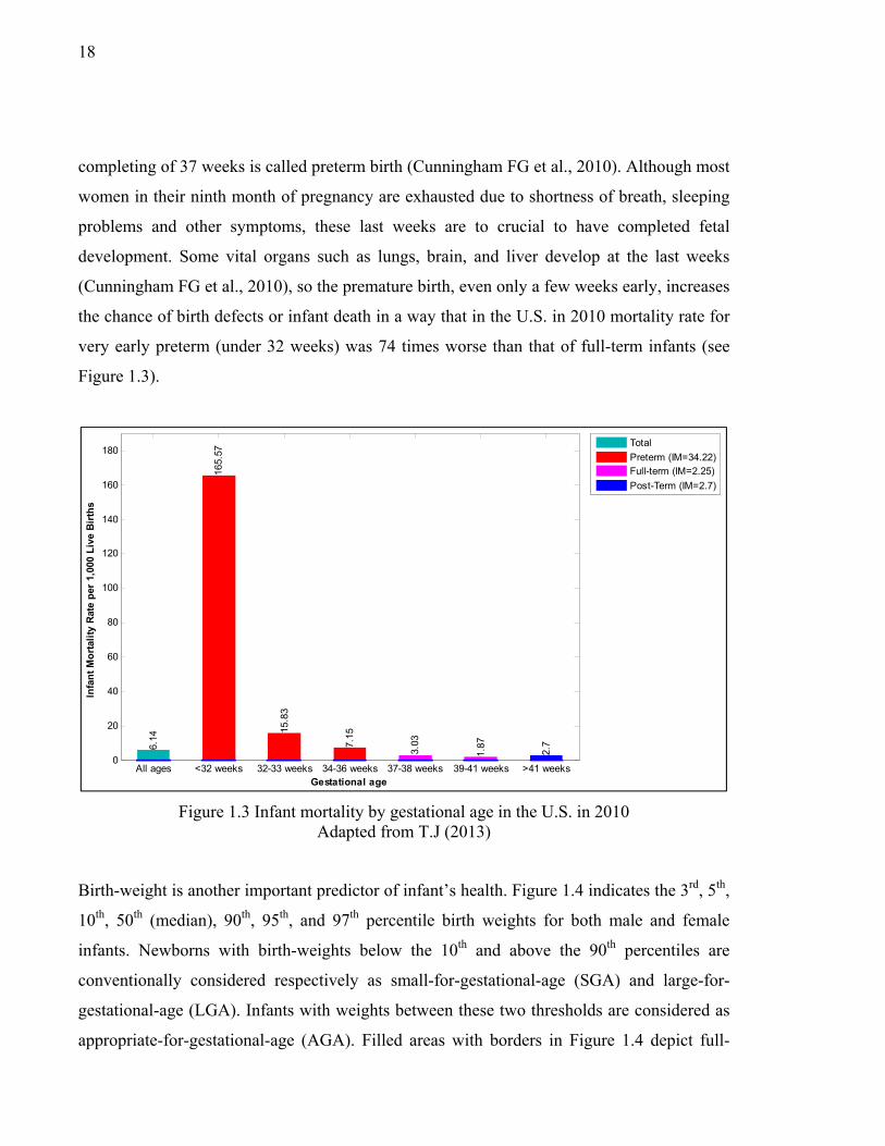
Gestational age is the noteworthy predictor of infant’s health condition with the normal range
of 37-41 weeks for babies which are fully developed (full-term). Any live birth before
18
completing of 37 weeks is called preterm birth (Cunningham FG et al., 2010). Although most
women in their ninth month of pregnancy are exhausted due to shortness of breath, sleeping
problems and other symptoms, these last weeks are to crucial to have completed fetal
development. Some vital organs such as lungs, brain, and liver develop at the last weeks
(Cunningham FG et al., 2010), so the premature birth, even only a few weeks early, increases
the chance of birth defects or infant death in a way that in the U.S. in 2010 mortality rate for
very early preterm (under 32 weeks) was 74 times worse than that of full-term infants (see
Figure 1.3).
Figure 1.3 Infant mortality by gestational age in the U.S. in 2010 Adapted from T.J (2013)
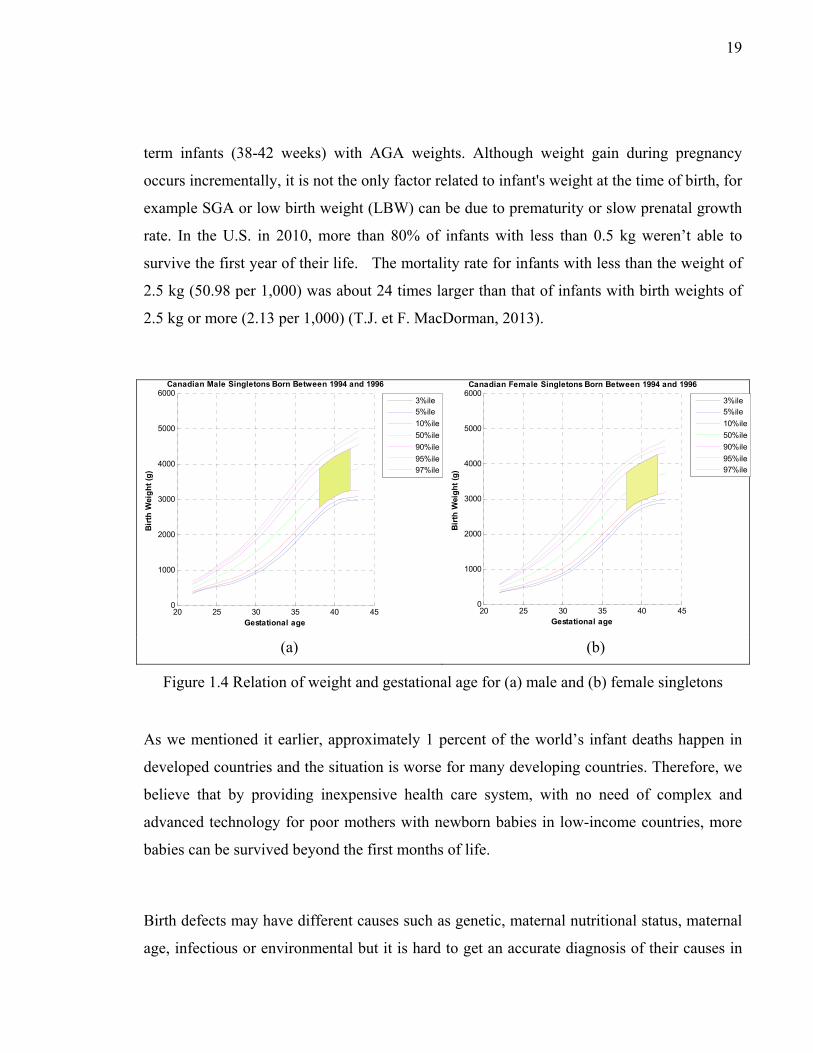
Birth-weight is another important predictor of infant’s health. Figure 1.4 indicates the 3rd, 5th,
10th, 50th (median), 90th, 95th, and 97th percentile birth weights for both male and female
infants. Newborns with birth-weights below the 10th and above the 90th percentiles are
conventionally considered respectively as small-for-gestational-age (SGA) and large-for-
gestational-age (LGA). Infants with weights between these two thresholds are considered as
appropriate-for-gestational-age (AGA). Filled areas with borders in Figure 1.4 depict full-
All ages <32 weeks 32-33 weeks 34-36 weeks 37-38 weeks 39-41 weeks >41 weeks0
20
40
60
80
100
120
140
160
180
Gestational age
Infa
nt M
orta
lity
Rate
per
1,0
00 L
ive
Birth
s
6.14
165.
57
15.8
3
7.15
3.03
1.87
2.7
Total
Preterm (IM=34.22)Full-term (IM=2.25)
Post-Term (IM=2.7)
19
term infants (38-42 weeks) with AGA weights. Although weight gain during pregnancy
occurs incrementally, it is not the only factor related to infant's weight at the time of birth, for
example SGA or low birth weight (LBW) can be due to prematurity or slow prenatal growth
rate. In the U.S. in 2010, more than 80% of infants with less than 0.5 kg weren’t able to
survive the first year of their life. The mortality rate for infants with less than the weight of
2.5 kg (50.98 per 1,000) was about 24 times larger than that of infants with birth weights of
2.5 kg or more (2.13 per 1,000) (T.J. et F. MacDorman, 2013).
(a) (b)
Figure 1.4 Relation of weight and gestational age for (a) male and (b) female singletons
As we mentioned it earlier, approximately 1 percent of the world’s infant deaths happen in
developed countries and the situation is worse for many developing countries. Therefore, we
believe that by providing inexpensive health care system, with no need of complex and
advanced technology for poor mothers with newborn babies in low-income countries, more
babies can be survived beyond the first months of life.
Birth defects may have different causes such as genetic, maternal nutritional status, maternal
age, infectious or environmental but it is hard to get an accurate diagnosis of their causes in
20 25 30 35 40 450
1000
2000
3000
4000
5000
6000
Gestational age
Birth
Wei
ght (
g)
Canadian Male Singletons Born Between 1994 and 1996
3%ile5%ile
10%ile
50%ile
90%ile
95%ile97%ile
20 25 30 35 40 450
1000
2000
3000
4000
5000
6000
Gestational age
Birth
Wei
ght (
g)
Canadian Female Singletons Born Between 1994 and 1996
3%ile5%ile
10%ile
50%ile
90%ile
95%ile97%ile

20
origin. However, for some known risk factors there are some primary prevention solutions
such as adequate use of antenatal care and vaccination. Congenital anomalies can affect any
part of the body such as brain, ears, and heart. However, it is easier to identify a baby with
structural problems such as cleft lip, but on the other hand, symptoms of other defects might
be invisible and hidden from sight.
These official statistics can provide more information about the chance of infants born with
specific congenital disease which is completely independent of the information inside infant
cries. Moreover, there are other independent sources of information related to the
physiological condition of newborn infants that can be useful like in a similar way in
multimodal biometric systems. However, in this article we are curious to examine only the
ability of information embedded in infant cries.
1.2.2 Primary research
Some of prior works have focused on analyzing different kinds of cries and trying to find
differences between them. A preliminary report of infant cry analysis in 1963, researchers
could distinguish 4 types of infant cry, namely the first birth cry, the hunger cry, the pain cry,
and the pleasure cry from each other both auditorily and by using of sound spectrography
(Wasz-Hockert et al., 1963).
Another group of researchers were interested in auditory identification of cry types by
training people who had had past experience with infant cries, such as midwives (Wasz-
Hockert, Michelsson et Lind, 1985). Additionally, in 1967 they found that cries of sick
infants could be distinguished auditorily as basic cry types, namely birth, hunger, pain, and
pleasure. Infants with asphyxia, brain damage, hyperbilirubinemia and, Down’s syndrome
were used in the research work (Partanen et al., 1967). Table 1.4 compares the results for the
hunger, birth, and pleasure cry. In these methods training phase plays a vital role in
improving the ability to recognize the cries.

21
Table 1.4 Similarities between hunger, first birth, and pleasure cry
Max
Pit
ch (
Hz)
Min
Pit
ch (
Hz)
Sh
ift
(occ
urr
ed in
%)
Mel
ody
Typ
e
Glo
ttal
Rol
l
(occ
urr
ed in
%)
Mea
n D
ura
tion
Hunger Cry 550 390 2% falling, rising /
falling in 80%
24% -
First Birth Cry 550 450 18% - - Short
(1.1 sec)
Pleasure Cry 650 360 19% flat in 46% 26% -
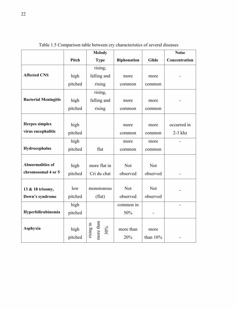
Many experiments on sick infants with various diseases have been done in order to make a
general assessment of the effect on cry characteristics. Table 1.5 depicts some cry
characteristics, such as pitch, melody type and the occurrence of biphonation and glide
change in sick infants (Wasz-Hockert, Michelsson et Lind, 1985).
Normal range of fundamental frequencies has been mentioned in papers between 400 and
600 Hz for healthy infants’ cries (Lind et Wermke, 2002). In addition, three cry features,
namely biphonation, glide, and shift, have been rarely found in the crying of healthy infants.
In contrast, abnormal high mean value of fundamental frequencies (F0>600 Hz) has been
reflected in crying of infant who suffer from CNS-disorders (Michelsson, 1971; Michelsson
et Michelsson, 1999).
The changes in cry characteristics in newborn infants with asphyxia were so apparent and the
results indicate that cry analysis has diagnostic value as well as prognostic value when
analyzing cries of infants with meningitis. As you can see in the Table 1.6 (Wasz-Hockert,
Michelsson et Lind, 1985), it is observed that the pitch and some other cry characteristics
change when the child is sick, especially the ones with central nervous system diseases. For
example, the latency of normal infants is less than that of infants with diffuse brain damage.
It means that healthy infants respond more quickly than others to stimuli.
22
Table 1.5 Comparison table between cry characteristics of several diseases
Pitch
Melody
Type
Biphonation
Glide
Noise
Concentration
Affected CNS high
pitched
rising,
falling and
rising
more
common
more
common
-
Bacterial Meningitis high
pitched
rising,
falling and
rising
more
common
more
common
-
Herpes simplex
virus encephalitis
high
pitched
more
common
more
common
occurred in
2-3 khz
Hydrocephalus
high
pitched flat
more
common
more
common
-
Abnormalities of
chromosomal 4 or 5
high
pitched
more flat in
Cri du chat
Not
observed
Not
observed
-
13 & 18 trisomy,
Down’s syndrome
low
pitched
monotonous
(flat)
Not
observed
Not
observed
-
Hyperbilirubinemia
high
pitched
common in
50% -
-
Asphyxia high
pitched risi
ng in
mor
e th
an
30%
more than
20%
more
than 10%
-

23
Table 1.6 Comparison table between cry characteristics of healthy and sick infants
Cry characteristics Healthy Sick
Brain damage Meningitis
CNS disorders
latency 1.2 s - 2.6 s - -
Duration 2.6-5.2 s - - 1.7 s -
Maximum Pitch
570-680 Hz , 650 greater - - -
Minimum Pitch
330-420 Hz greater - - -
Shift ever
y th
ird
pain
cry
1-
2 kH
z
- - -
high
-pi
tche
d sh
ift
Melody Type fall
ing
or
risi
ng /
fall
ing
- - -
risi
ng
and
fall
ing/
risi
ng
Glottal Roll rela
tive
ly c
omm
on
at th
e en
d of
the
phon
atio
ns,1
8% to
73
% o
f cr
ies
less
com
mon
due
to
shor
ter
cry
and
end
abru
ptly
- - -
Biphonation extr
emel
y ra
re
- - - espe
cial
ly
pres
ent i
n th
is
dise
ase
Glide extr
emel
y ra
re
Mostly - - pres
ent i
n th
is
dise
ase
Noise concentration ex
trem
ely
rare
- - - -

24
1.2.3 Early-infant medical researches
Here, we will very briefly define some standard measure as specificity and sensitivity. These
measures are computed from true positive (TP), true negative (TN), false positive (FP), and false
negative (FN) as presented in Table 1.7.
= ( + ) (1.1)
= ( + ) (1.2)
= +( + + + ) (1.3)
and:
• TP = true positive, the classifier classified as pathology when pathological samples
were present;
• TN = true negative, the classifier classified as normal when normal samples were
present;
• FN = false negative, the classifier classified as normal when pathological samples were
present;
• FP = false positive, the classifier classified as pathological when normal samples were
present.
Table 1.7 Confusion matrix
Actual classification Predicted classification
Pathological Normal
Pathological TP FN
Normal FP TN

25
The medical research into infant cry signals is divided into three main areas:
1. Severe pathology and medical problems such as Asphyxia which may be identified by
existing techniques and tests (see Table 1.8, (Benson et Haith, 2009));
2. Diseases and medical problems such as SIDS that are currently undetectable until it is too
late for treatment (see Table 1.9, (Benson et Haith, 2009));
3. Medical conditions which place the infants at risk for poor outcome but the prognosis is
not clear such as prenatal exposure to illegal drugs or premature infants (see Table 1.9,
(Benson et Haith, 2009)).
Table 1.8 Cry features of infants with severe pathologies
For diagnosis of medical syndromes or damage to the CNS, the most common changes in cry
characteristics are higher and more variability in it. In case of one of these significant
medical problems, there are often other clinical signs. Nonetheless there is no doubt that this
Medical Condition Cry Characteristic
Asphyxia ↑F0, ↑ F0 instability, biphonation, ↑sub-harmonic break, ↓
duration
Brain damage ↑F0, ↑ F0 instability, biphonation , ↑ threshorld, ↓ duration,
↑ latency, ↑ short utterances.
Cri du chat ↑F0
Down Syndrome ↑F0, ↑ F0 instability , ↓ intensity (amplitude )
Hydrocéphalus ↑F0, ↑ F0 instability , ↓ latence
Hypothyroïdism ↓F0
Krabbe’s disease ↑F0
Meningitis bacterial ↑F0, F0 instability, biphonation , ↓ duration
Trisomie 13,18, 21 ↓F0

26
sort of help could be valuable for infants already diagnosed with CNS damages. For example,
in some cases with severe asphyxia or bacterial meningitis infants had the poorest prognoses.
For health problems that are not detectable by available medical examinations such as SIDS,
it is worthwhile to look for some cry characteristics associated with medical problems.
Limited previous works has shown that infants with vocal constriction (high ) and poor
control over the vocal tract (increased cry mode changes) are more likely to die of SIDS.
Briefly Table 1.9depicts cry characteristics observed in infants who are at-risk (Benson et
Haith, 2009).
Some experiments have been carried out on infants of mothers who abused a variety of
substances, namely alcohol, tobacco, and cocaine during pregnancy (Corwin, Lester et
Golub, 1996). The cry characteristics of these infants also have been shown to be abnormal
in comparison to healthy infants.
172 healthy infants have been under studied according to their gender separately in
(Michelsson et al., 2002) and no significant differences between cry characteristics such as
melody type, and mean value of maximum/minimum of the fundamental frequency have
been noted. The same result has been achieved for babies in different ages (1-7 days old) or
the gestational age when they were born. On the contrary of former studies (Gilbert et Robb,
1996; Prescott, 1975), no significant weekly changes were found in (Lind et Wermke, 2002)
during the first three months of life. As you can see in Figure 1.5, there is no marked increase
or decrease in .
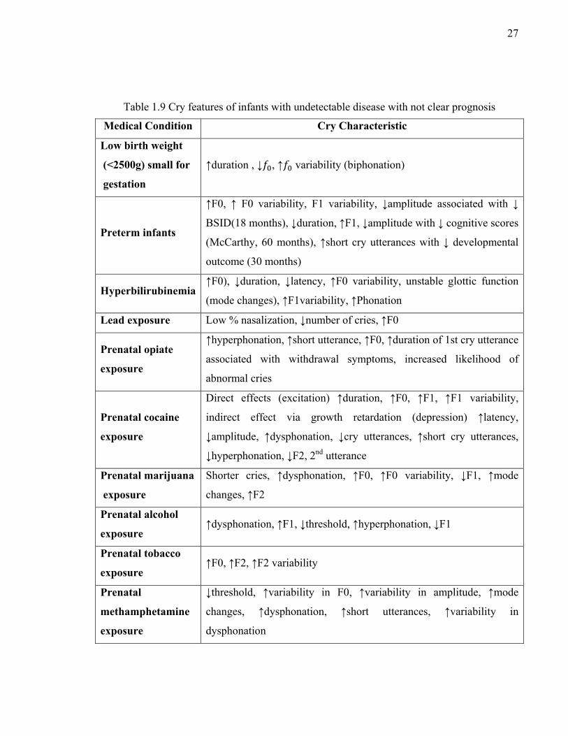
27
Table 1.9 Cry features of infants with undetectable disease with not clear prognosis
Medical Condition Cry Characteristic
Low birth weight
(<2500g) small for
gestation
↑duration , ↓ , ↑ variability (biphonation)
Preterm infants
↑F0, ↑ F0 variability, F1 variability, ↓amplitude associated with ↓
BSID(18 months), ↓duration, ↑F1, ↓amplitude with ↓ cognitive scores
(McCarthy, 60 months), ↑short cry utterances with ↓ developmental
outcome (30 months)
Hyperbilirubinemia ↑F0), ↓duration, ↓latency, ↑F0 variability, unstable glottic function
(mode changes), ↑F1variability, ↑Phonation
Lead exposure Low % nasalization, ↓number of cries, ↑F0
Prenatal opiate
exposure
↑hyperphonation, ↑short utterance, ↑F0, ↑duration of 1st cry utterance
associated with withdrawal symptoms, increased likelihood of
abnormal cries
Prenatal cocaine
exposure
Direct effects (excitation) ↑duration, ↑F0, ↑F1, ↑F1 variability,
indirect effect via growth retardation (depression) ↑latency,
↓amplitude, ↑dysphonation, ↓cry utterances, ↑short cry utterances,
↓hyperphonation, ↓F2, 2nd utterance
Prenatal marijuana
exposure
Shorter cries, ↑dysphonation, ↑F0, ↑F0 variability, ↓F1, ↑mode
changes, ↑F2
Prenatal alcohol
exposure ↑dysphonation, ↑F1, ↓threshold, ↑hyperphonation, ↓F1
Prenatal tobacco
exposure ↑F0, ↑F2, ↑F2 variability
Prenatal
methamphetamine
exposure
↓threshold, ↑variability in F0, ↑variability in amplitude, ↑mode
changes, ↑dysphonation, ↑short utterances, ↑variability in
dysphonation
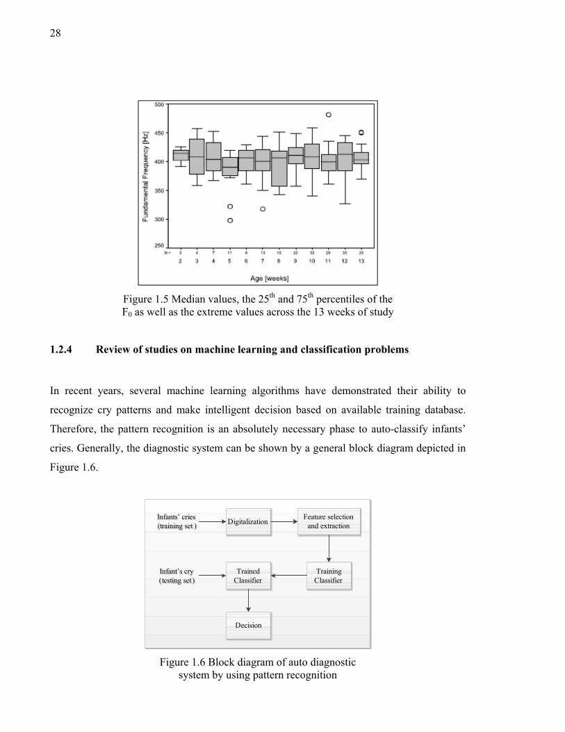
28
Figure 1.5 Median values, the 25th and 75th percentiles of the F0 as well as the extreme values across the 13 weeks of study
1.2.4 Review of studies on machine learning and classification problems
In recent years, several machine learning algorithms have demonstrated their ability to
recognize cry patterns and make intelligent decision based on available training database.
Therefore, the pattern recognition is an absolutely necessary phase to auto-classify infants’
cries. Generally, the diagnostic system can be shown by a general block diagram depicted in
Figure 1.6.
Infants’ cries (training set )Infants’ cries (training set )
DigitalizationFeature selection
and extraction
Training Classifier
Trained Classifier
Infant’s cry (testing set)Infant’s cry (testing set)
Decision
Figure 1.6 Block diagram of auto diagnostic system by using pattern recognition
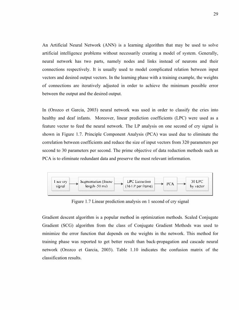
29
An Artificial Neural Network (ANN) is a learning algorithm that may be used to solve
artificial intelligence problems without necessarily creating a model of system. Generally,
neural network has two parts, namely nodes and links instead of neurons and their
connections respectively. It is usually used to model complicated relation between input
vectors and desired output vectors. In the learning phase with a training example, the weights
of connections are iteratively adjusted in order to achieve the minimum possible error
between the output and the desired output.
In (Orozco et Garcia, 2003) neural network was used in order to classify the cries into
healthy and deaf infants. Moreover, linear prediction coefficients (LPC) were used as a
feature vector to feed the neural network. The LP analysis on one second of cry signal is
shown in Figure 1.7. Principle Component Analysis (PCA) was used due to eliminate the
correlation between coefficients and reduce the size of input vectors from 320 parameters per
second to 30 parameters per second. The prime objective of data reduction methods such as
PCA is to eliminate redundant data and preserve the most relevant information.
Figure 1.7 Linear prediction analysis on 1 second of cry signal
Gradient descent algorithm is a popular method in optimization methods. Scaled Conjugate
Gradient (SCG) algorithm from the class of Conjugate Gradient Methods was used to
minimize the error function that depends on the weights in the network. This method for
training phase was reported to get better result than back-propagation and cascade neural
network (Orozco et Garcia, 2003). Table 1.10 indicates the confusion matrix of the
classification results.
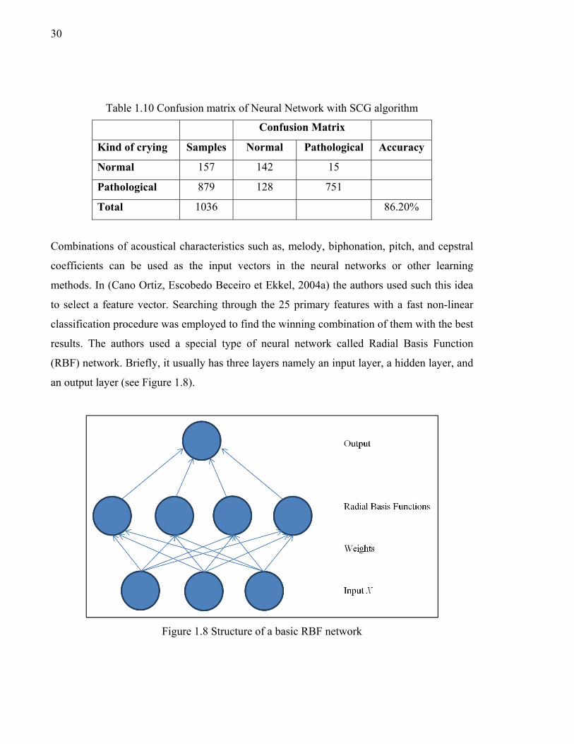
30
Table 1.10 Confusion matrix of Neural Network with SCG algorithm
Confusion Matrix
Kind of crying Samples Normal Pathological Accuracy
Normal 157 142 15
Pathological 879 128 751
Total 1036 86.20%
Combinations of acoustical characteristics such as, melody, biphonation, pitch, and cepstral
coefficients can be used as the input vectors in the neural networks or other learning
methods. In (Cano Ortiz, Escobedo Beceiro et Ekkel, 2004a) the authors used such this idea
to select a feature vector. Searching through the 25 primary features with a fast non-linear
classification procedure was employed to find the winning combination of them with the best
results. The authors used a special type of neural network called Radial Basis Function
(RBF) network. Briefly, it usually has three layers namely an input layer, a hidden layer, and
an output layer (see Figure 1.8).
Figure 1.8 Structure of a basic RBF network
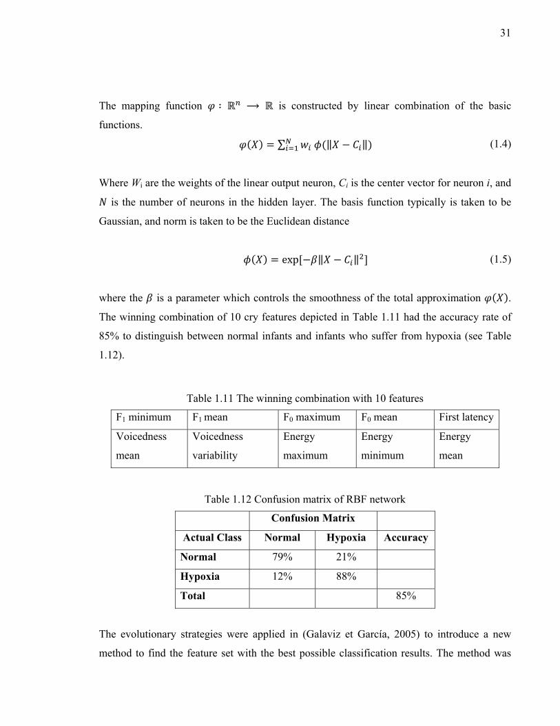
31
The mapping function ∶ ℝ ⟶ ℝ is constructed by linear combination of the basic
functions.
( ) = ∑ (‖ − ‖) (1.4)
Where Wi are the weights of the linear output neuron, Ci is the center vector for neuron i, and
is the number of neurons in the hidden layer. The basis function typically is taken to be
Gaussian, and norm is taken to be the Euclidean distance
( ) = exp[− ‖ − ‖ ] (1.5)
where the is a parameter which controls the smoothness of the total approximation ( ). The winning combination of 10 cry features depicted in Table 1.11 had the accuracy rate of
85% to distinguish between normal infants and infants who suffer from hypoxia (see Table
1.12).
Table 1.11 The winning combination with 10 features
F1 minimum F1 mean F0 maximum F0 mean First latency
Voicedness
mean
Voicedness
variability
Energy
maximum
Energy
minimum
Energy
mean
Table 1.12 Confusion matrix of RBF network
Confusion Matrix
Actual Class Normal Hypoxia Accuracy
Normal 79% 21%
Hypoxia 12% 88%
Total 85%
The evolutionary strategies were applied in (Galaviz et García, 2005) to introduce a new
method to find the feature set with the best possible classification results. The method was
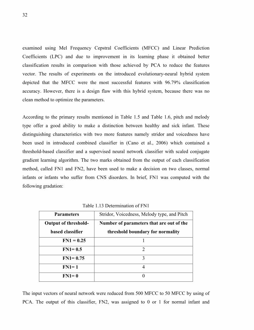
32
examined using Mel Frequency Cepstral Coefficients (MFCC) and Linear Prediction
Coefficients (LPC) and due to improvement in its learning phase it obtained better
classification results in comparison with those achieved by PCA to reduce the features
vector. The results of experiments on the introduced evolutionary-neural hybrid system
depicted that the MFCC were the most successful features with 96.79% classification
accuracy. However, there is a design flaw with this hybrid system, because there was no
clean method to optimize the parameters.
According to the primary results mentioned in Table 1.5 and Table 1.6, pitch and melody
type offer a good ability to make a distinction between healthy and sick infant. These
distinguishing characteristics with two more features namely stridor and voicedness have
been used in introduced combined classifier in (Cano et al., 2006) which contained a
threshold-based classifier and a supervised neural network classifier with scaled conjugate
gradient learning algorithm. The two marks obtained from the output of each classification
method, called FN1 and FN2, have been used to make a decision on two classes, normal
infants or infants who suffer from CNS disorders. In brief, FN1 was computed with the
following gradation:
Table 1.13 Determination of FN1
Parameters Stridor, Voicedness, Melody type, and Pitch
Output of threshold-
based classifier
Number of parameters that are out of the
threshold boundary for normality
FN1 = 0.25 1
FN1= 0.5 2
FN1= 0.75 3
FN1= 1 4
FN1= 0 0
The input vectors of neural network were reduced from 500 MFCC to 50 MFCC by using of
PCA. The output of this classifier, FN2, was assigned to 0 or 1 for normal infant and
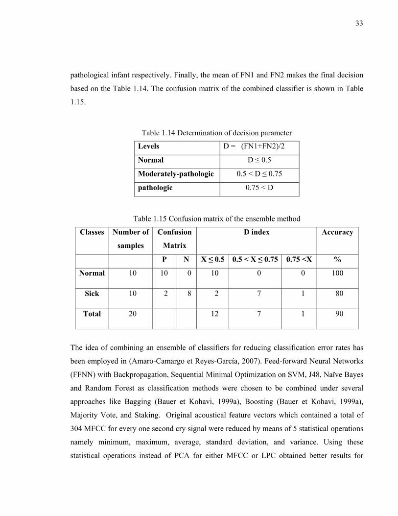
33
pathological infant respectively. Finally, the mean of FN1 and FN2 makes the final decision
based on the Table 1.14. The confusion matrix of the combined classifier is shown in Table
1.15.
Table 1.14 Determination of decision parameter
Levels D = (FN1+FN2)/2
Normal D ≤ 0.5
Moderately-pathologic 0.5 < D ≤ 0.75
pathologic 0.75 < D
Table 1.15 Confusion matrix of the ensemble method
Classes Number of
samples
Confusion
Matrix
D index Accuracy
P N X ≤ 0.5 0.5 < X ≤ 0.75 0.75 <X %
Normal 10 10 0 10 0 0 100
Sick 10 2 8 2 7 1 80
Total 20 12 7 1 90
The idea of combining an ensemble of classifiers for reducing classification error rates has
been employed in (Amaro-Camargo et Reyes-García, 2007). Feed-forward Neural Networks
(FFNN) with Backpropagation, Sequential Minimal Optimization on SVM, J48, Naïve Bayes
and Random Forest as classification methods were chosen to be combined under several
approaches like Bagging (Bauer et Kohavi, 1999a), Boosting (Bauer et Kohavi, 1999a),
Majority Vote, and Staking. Original acoustical feature vectors which contained a total of
304 MFCC for every one second cry signal were reduced by means of 5 statistical operations
namely minimum, maximum, average, standard deviation, and variance. Using these
statistical operations instead of PCA for either MFCC or LPC obtained better results for
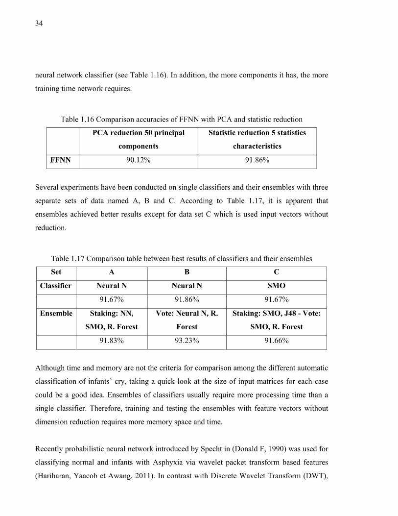
34
neural network classifier (see Table 1.16). In addition, the more components it has, the more
training time network requires.
Table 1.16 Comparison accuracies of FFNN with PCA and statistic reduction
PCA reduction 50 principal
components
Statistic reduction 5 statistics
characteristics
FFNN 90.12% 91.86%
Several experiments have been conducted on single classifiers and their ensembles with three
separate sets of data named A, B and C. According to Table 1.17, it is apparent that
ensembles achieved better results except for data set C which is used input vectors without
reduction.
Table 1.17 Comparison table between best results of classifiers and their ensembles
Set A B C
Classifier Neural N Neural N SMO
91.67% 91.86% 91.67%
Ensemble Staking: NN,
SMO, R. Forest
Vote: Neural N, R.
Forest
Staking: SMO, J48 - Vote:
SMO, R. Forest
91.83% 93.23% 91.66%
Although time and memory are not the criteria for comparison among the different automatic
classification of infants’ cry, taking a quick look at the size of input matrices for each case
could be a good idea. Ensembles of classifiers usually require more processing time than a
single classifier. Therefore, training and testing the ensembles with feature vectors without
dimension reduction requires more memory space and time.
Recently probabilistic neural network introduced by Specht in (Donald F, 1990) was used for
classifying normal and infants with Asphyxia via wavelet packet transform based features
(Hariharan, Yaacob et Awang, 2011). In contrast with Discrete Wavelet Transform (DWT),

35
both lower and higher frequency bands are decomposed into 2 sub-bands in wavelet packet
transform. The decomposition coefficient of the i-th depth was computed and frequency
ranges of subspaces in each level of decomposition can be calculated as below:
0, , , , , … , ( ) , , (1.6)
After 5 levels of decomposition, the sub-band energy and entropy were computed from
wavelet packet coefficients by the following equations.
= ∑ , = 1,2, … , , = 0,1,… , 2 − 1 (1.7)
= ∑ , , , = 1,2, … , , = 0,1, … ,2 − 1 (1.8)
where P is the scale index, n is number of decomposition level. Several experiments have
been done with different level of wavelet packet decomposition, and the results in Table 1.18
depicted that the highest achievable classification accuracy of 99% was obtained at the fifth
level of decomposition.
1.3 Cry pattern classification
This section discusses briefly the idea behind choosing the proposed machine learning
methodology and other related issues from different point of views.
Generally we can consider the solution of our classification problem in two different ways:
Set up a multi-class classification problem or treat each classification problem independently
like a one-class or binary classification. One is not necessarily better, there are trade-offs.
First of all, many good classifiers like logistic regression can only handle binary
classification problem. So if we want to use it for multi-class problems, we have to turn it
into a set of binary classification problems.
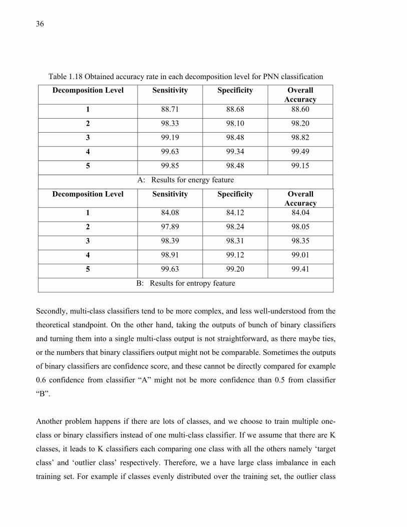
36
Table 1.18 Obtained accuracy rate in each decomposition level for PNN classification
Decomposition Level Sensitivity Specificity Overall Accuracy
1 88.71 88.68 88.60
2 98.33 98.10 98.20
3 99.19 98.48 98.82
4 99.63 99.34 99.49
5 99.85 98.48 99.15
A: Results for energy feature
Decomposition Level Sensitivity Specificity Overall Accuracy
1 84.08 84.12 84.04
2 97.89 98.24 98.05
3 98.39 98.31 98.35
4 98.91 99.12 99.01
5 99.63 99.20 99.41
B: Results for entropy feature
Secondly, multi-class classifiers tend to be more complex, and less well-understood from the
theoretical standpoint. On the other hand, taking the outputs of bunch of binary classifiers
and turning them into a single multi-class output is not straightforward, as there maybe ties,
or the numbers that binary classifiers output might not be comparable. Sometimes the outputs
of binary classifiers are confidence score, and these cannot be directly compared for example
0.6 confidence from classifier “A” might not be more confidence than 0.5 from classifier
“B”.
Another problem happens if there are lots of classes, and we choose to train multiple one-
class or binary classifiers instead of one multi-class classifier. If we assume that there are K
classes, it leads to K classifiers each comparing one class with all the others namely ‘target
class’ and ‘outlier class’ respectively. Therefore, we a have large class imbalance in each
training set. For example if classes evenly distributed over the training set, the outlier class

37
will have K-1 times as many samples as the target class. We should be well aware of class
imbalance, since it would have an adverse impact on the performance of many classifiers.
So finally, neither one is necessarily better. It is a better idea to try both practically and see
which performance is better for our particular case.
1.3.1 Brief description on various classifiers
A brief description and comparison of the various classifiers that have been used in past
studies like Artificial Neural Network (ANN), Support Vector Machine (SVM) are given
below.
1.3.1.1 ANN and SVM
We have a fairly similar case in ANN in which two options are presented; separate networks
for each binary classification or train one network with one output for each binary
classification, but with a shared hidden layer. Using a shared hidden layer could be a clever
idea to have all scores on a same scale and solve comparability of classifiers score.
Nevertheless, having some networks is not always preferable over the one network with
shared hidden layer. In the case with shared hidden layer and more output nodes, the network
needs a larger hidden layer, as the learning function gets more complex. A larger hidden
layer means we are more prone to overfitting, so we'll need more training data. However, as
above, figuring out how to turn the output of k networks into a single k-class output is not an
easy task.
The development of ANN followed a heuristic path, with applications and extensive
experimentation preceding theory. In contrast, the development of SVMs involved sound
theory first, then implementation and experiments. A significant advantage of SVMs is that
whilst neural networks can suffer from multiple local minima, the solution to an SVM is
global and unique. Two more advantages of SVMs are simple geometric interpretation and
38
sparse solution. Moreover, unlike neural networks, the computational complexity of SVMs
does not depend on the dimensionality of the input space. Neural networks use empirical risk
minimization, whilst SVMs use structural risk minimization. The reason that SVMs often
outperform neural networks in practice is that the SVMs are less prone to overfitting. The
key features of SVMs are the use of kernels, the absence of local minima, the sparseness of
the solution and the capacity control obtained by optimizing the margin.
A common disadvantage of non-parametric techniques such as SVMs is the lack of
transparency of results. SVMs cannot represent the score of all companies as a simple
parametric function of the financial ratios, since its dimension may be very high. It is neither
a linear combination of single financial ratios nor has it another simple functional form. The
weights of the financial ratios are not constant. Thus the marginal contribution of each
financial ratio to the score is variable. Using a Gaussian kernel each company has its own
weights according to the difference between the value of their own financial ratios and those
of the support vectors of the training data sample. An important practical question that is not
entirely solved is the selection of the kernel function parameters. The most serious problem
with SVMs is the high algorithmic complexity and extensive memory requirements of the
required quadratic programming in large-scale tasks. Here are some disadvantages of SVM:
1. Computationally demanding to train and run;
2. Sensitive to noisy data;
3. Prone to over fitting and thus bad generalization;
4. Choice of kernel function and the parameters have to be set manually and can greatly
impact the results.

39
Here are some advantages and disadvantages of Neural Network classifiers.
Advantages:
1. Powerful non-linear classifier;
2. Elegant solutions built of continuous basis-functions;
3. Handles noisy data well;
4. Fast to run.
Disadvantages:
1. Computationally demanding to train;
2. With difficulty when there is complex boundary.
1.3.1.2 Decision tree
The decision tree is a class discriminator that recursively partitions the training set until each
partition consists entirely or dominantly of examples from one class. Each non-leaf node of
the tree contains a split point that is a test on one or more attributes and determines how the
data is partitioned. The decision trees are easy to understand and modify, and the model
developed can be expressed as a set of decision rules. This algorithm scales well, even where
there are varying numbers of training examples and considerable numbers of attributes in
large databases. The decision tree model contains rules to predict the target variable and it
provides an easy-to-understand description of the underlying distribution of the data. It can
be constructed relatively quickly, compared to other methods. Moreover it can process both
numerical and categorical data. The process of pruning the initial tree consists of removing
small, deep nodes of the tree resulting from 'noise' contained in the training data, thus

40
reducing the risk of overfitting, and resulting in a more accurate classification of unknown
data. Some disadvantages of the decision tree classifier are mentioned in below:
1. Categorical output attribute;
2. Limited to one output attribute;
3. Unstable algorithms;
4. Complex trees created from numeric datasets;
5. Over-sensitivity to the training set, irrelevant attributes and noise.
1.3.1.3 Naïve Bayes
A Naïve Bayes classifier is a simple probabilistic classifier based on applying Bayes'
theorem with strong (naive) independence assumptions. In simple terms, the Naïve Bayes
classifier assumes that the presence (or absence) of a particular feature of a class is unrelated
to the presence (or absence) of any other feature, given the class variable. Depending on the
precise nature of the probability model, naive Bayes classifiers can be trained very efficiently
in a supervised learning setting. In many practical applications, parameter estimation for
naive Bayes models uses the method of maximum likelihood. An advantage of the naive
Bayes classifier is that it only requires a small amount of training data to estimate the
parameters necessary for classification. Since variables are assumed to be independent, only
the variances of the variables for each class need are determined not the entire covariance
matrix. However, it is not capable of solving complex classification problems.

41
1.3.1.4 K-nearest neighbor
K-Nearest Neighbor (K-NN) is very simple to understand and easy to implement. So it
should be considered in seeking a solution to any classification problem. The process is
transparent, it is easy to implement and debug. There are some noise reduction techniques
that work only for k-NN that can be effective in improving the accuracy of the classifier.
Most important disadvantages of KNN are as follows:
1. Because all the work is done at run-time, K-NN can have poor run-time performance if
the training set is large;
2. K-NN is very sensitive to irrelevant or redundant features because all features contribute
to the similarity and thus to the classification. This can be ameliorated by careful feature
selection or feature weighting;
3. On very difficult classification tasks, K-NN may be outperformed by more exotic
techniques such as SVMs or Neural Networks.
1.3.2 Why Gaussian Mixture Models?
The classical uni-modal Gaussian model represents feature distributions by a position (mean
vector) and an elliptic shape (covariance matrix) and a vector quantization (VQ) or nearest
neighbor model represents a distribution by a discrete set of characteristic templates. The
GMM acts as a hybrid between these two models by using a discrete set of Gaussian
functions, each with their own mean and covariance matrix, to allow a better modeling
capability. Figure 1.9 compares the densities obtained using a uni-modal Gaussian model,
the GMM and VQ model. Plot (a) shows the histogram of a single feature from a speaker
recognition system (a single cepstral value from a 25 second utterance by a male speaker);
plot (b) shows a uni-modal Gaussian model of this feature distribution; plot (c) shows the
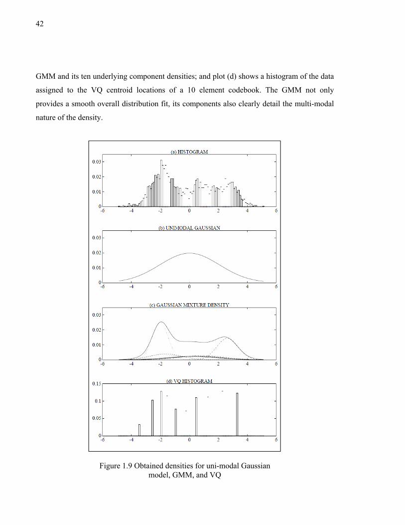
42
GMM and its ten underlying component densities; and plot (d) shows a histogram of the data
assigned to the VQ centroid locations of a 10 element codebook. The GMM not only
provides a smooth overall distribution fit, its components also clearly detail the multi-modal
nature of the density.
Figure 1.9 Obtained densities for uni-modal Gaussian model, GMM, and VQ
43
Experimental results of the GMM have shown that its accuracy is higher than those obtained
by the VQ approach, the Radial Basis Function network model (RBF), and also the learning
Vector Quantization (LVQ) approach. Moreover, the training time of the GMM is less than
that of Multilayer Perceptron (MLP) (Ma et Gao, 1998). The GMM trained with the EM
learning algorithm has comparable flexibility with the multilayer perceptron in modeling
non-stationary, multimodal machine signal characteristics, but has significantly fewer
parameters to train (Heck et Chou, 1994).
Moreover, the GMM has the capability to form smooth approximations to arbitrarily shaped
densities and it has proved to be an effective probabilistic model for a lot of application such
as biometric systems, most notably in speaker recognition systems and speaker identification
(Reynolds et Rose, 1995) due to their capability of representing a large class of sample
distributions. The GMM represents a statistical pattern recognition approach that enables
optimal processing of data both for training the classifier (the EM algorithm) and for
performing on-line classification. In addition, while the GMMs possess many discriminant
surface-modeling capabilities of more complex nonparametric classifiers (e.g., multilayered
perceptrons), the GMM is parametric, making it more robust to the effects of a limited
amount of training data (Heck et Chou, 1994).
1.3.2.1 Introduction to GMMs
Gaussian Mixture Model as a parametric probability density function is chosen to model
infants’ cry under available pathological states. A complete GMM for a D dimensional
continuous value data vector called X can be represented by λ = w , μ , Σ i = 1,… ,M as a
weighted sum of M Gaussian component densities as follow:
F (X|λ) = ∑ w f (X|μ , Σ ) , ∑ w = 1 (1.9)
where w , μ , Σ are the mixture weights, mean vector and covariance matrix respectively.
Since GMMs is used usually in unsupervised learning and clustering problem which the
44
number of mixtures and parameter vectors μ , Σ are unknown, the choice of model
configuration is almost determined by the amount of data available for estimating the GMM
parameters in a particular application.
The GMM can also be viewed as a single-state HMM with a Gaussian mixture observation
density, or an ergodic Gaussian observation HMM with fixed, equal transition probabilities.
Assuming independent feature vectors, the observation density of feature vectors drawn from
these hidden acoustic classes is a Gaussian mixture. It is also important to note that in case of
statistically dependent features, the effect of using a set of M full covariance matrix
Gaussians can be equally obtained by using a larger set of diagonal covariance Gaussians,
due largely to that the linear combination of diagonal covariance basis Gaussians is capable
of modeling the correlations between feature vector elements. Therefore, there is significant
difference between Supervised Learning GMM (SLGMM) (Ma et Gao, 1998) and
unsupervised learning GMMs.
1.3.2.2 Learning of GMMs
Given training data and a GMM configuration, we wish to estimate the parameters of the
GMM, λ, which in some sense best matches the distribution of the training feature vectors.
The GMM parameters λ = w , μ , Σ are usually estimated from training data using the
iterative Expectation-Maximization (EM) algorithm or Maximum a-Posteriori (MAP)
estimation from a well-trained prior model. There are several techniques available for
estimating the parameters of the GMM but by far the most popular and well-established
method is maximum likelihood (ML) estimation. The aim of ML estimation is to find the
model parameters which maximize the likelihood of the GMM given the training data. For a
sequence of T training vectors X = (x , . . . , x ), the GMM likelihood, assuming
independence between the vectors, can be written as,
P(X|λ) = ∏ P(x |λ) (1.10)

45
Unfortunately, this expression is a non-linear function of the parameters λ and direct
maximization is not possible. However, ML parameter estimates can be obtained iteratively
using a special case of the EM algorithm. The iterative procedure in the EM algorithm
ensures that likelihood function doesn’t decrease per iteration. Consequently it yields locally
optimal, maximum likelihood parameter estimates. The EM begins with an initial model
called . Next, a new model is created after updating all parameters in such a way that ( | ) ≥ ( | ). This process is repeated until convergence.
If all goes well, the algorithm converges to local maximum (Heck et Chou, 1994), but there
are still some problems when increasing model complexity. Firstly, there is no guarantee that
the newly added mixture from random splitting always increases the likelihood function prior
to re-estimation. Secondly, convergence to the optimum point in EM-based re-estimation is
not be guaranteed due to sensitivity to initial parameters of the randomly split Gaussians. So
it is not the optimal manner of the model estimation (Jun, Yu et Hui, 2011).
A new method based on combination of Genetic Algorithm and the EM algorithm introduced
which has a better performance in the practical Brain Computer Interface (BCI) application,
due to reduce the negative effect of noisy data or outliers available in database (Boyu et al.,
2010).
In ASR system usually Gaussian mixtures HMMs are used as acoustic models in order to
model basic speech units. To deal with data sparseness problem in model training, the
mixing-up step is used to little by little increase the number of mixtures in each tied HMM
state to achieve the optimum performance. In such this ASR system, like HTK, the mixing-
up process is conducted in two steps (Young et al., 2006b) First of all, all existing Gaussians
or the most dominant Gaussian mixtures component in a HMM state is split up based on
some random or heuristic strategies. Second, all of these split Gaussians are re-estimated
based on the EM algorithm. Although it is a good strategy to learn models without getting
trapped in any bad local optimum, there are still some aforementioned problems when
increasing model complexity.
46
Recently another new method called Boosted Mixture Learning (BML) to learn Gaussian
mixture HMM is introduced (Jun, Yu et Hui, 2011). The new method called Boosted Mixture
Learning (BML) could be used as a successful candidate for training a GMM with some
adaptation in our case, due in part to its ability to rectify and overcome the aforementioned
problems in available techniques for estimating the GMM parameters.
1.3.2.3 Boosting algorithm
Generally, boosting method combines weak learners in a weighted majority voting scheme to
improve the overall classification accuracy for almost any type of learning algorithm. The
base classifiers, known also as weak learners, are trained using a weighted form of data set in
which the weighting coefficients associated with each data point depends on the performance
of the previous classifier. Therefore base classifiers are trained in sequence and the points
that are misclassified by one of the base classifiers are given greater weight when used to
train the next classifiers in the sequence. Using the updated training weights, a new classifier
is trained to concentrate more on these hard examples.
The main idea of boosting is that instead of always treating all data points as equal,
component classifiers should specialize on certain examples. In particular, if an example is
hard-to-classify and problematic for existing classifier, more components should focus on it.
According to the boosting theory, upper bound on training error rate is analytically
minimized. Moreover, some recent work has shown that boosting method can effectively
increase the margin of all training samples that can be explained by a theoretical view related
to functional gradient techniques (Jun, Yu et Hui, 2011). More recently, the traditional
boosting method has been used to solve some problems of mixture models (Kim et Pavlovic,
2007; Pavlovic, 2004).
47
1.4 Brief objectives, methodologies and contributions
Our general objective is to design a non-invasive cry-based diagnostic tool using computer
acoustical analysis of newborn cries to detect serious medical conditions such as heart
defects and infections. The diagram demonstrating the proposed system is shown below (see
Figure 1.10). It can interpret recorded cries to help neonatologists detect specific pathologies
affecting newborns since cry production in newborns can be influenced by neurological and
physiological states.
Our research team in the Multimodal-Modelisation-Specification (MMS) laboratory, located
at École de technologie supérieure (ÉTS), consists of three members. Their roles on the
research problem are explained briefly in below.
Mrs. Yasmina Kheddache, a PhD graduate from ÉTS, has worked on spectrographic analysis
of newborn infant cry signals to model newborn infant cry signals by parameters that
describe vocal cords and vocal tract. To achieve this objective, she proceeded to a qualitative
characterization of the cries of sick and healthy infants. For this purpose she used predefined
characteristics from literature that describe the behavior of cords and vocal tract during the
cry. For extraction of selected features, she implemented the methods of effective measures
to overcome the overestimation and underestimation of characteristics.
Mrs. Lina Abou-Abbas, pursuing a PhD degree, is working on the automatic segmentation of
newborn’s cry signals recorded in real conditions based on Hidden Markov Models using the
HTK (Hidden Markov Model Toolkit). The purpose of signal segmentation is to differentiate
the important acoustic parts of the cry recordings from the unimportant acoustic activities
that compose the audio signals.
In order to make a high accuracy decision in our diagnostic system, we should have had a
good understanding of different methods to create a pattern for cry signals. During my PhD
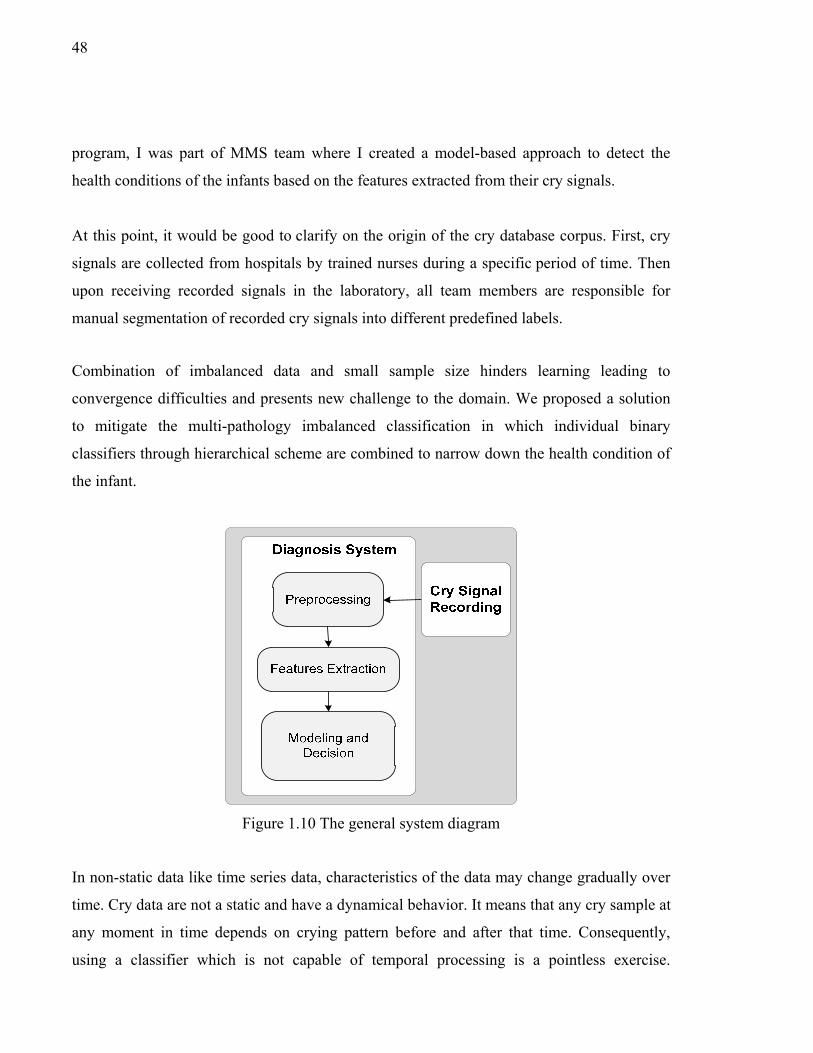
48
program, I was part of MMS team where I created a model-based approach to detect the
health conditions of the infants based on the features extracted from their cry signals.
At this point, it would be good to clarify on the origin of the cry database corpus. First, cry
signals are collected from hospitals by trained nurses during a specific period of time. Then
upon receiving recorded signals in the laboratory, all team members are responsible for
manual segmentation of recorded cry signals into different predefined labels.
Combination of imbalanced data and small sample size hinders learning leading to
convergence difficulties and presents new challenge to the domain. We proposed a solution
to mitigate the multi-pathology imbalanced classification in which individual binary
classifiers through hierarchical scheme are combined to narrow down the health condition of
the infant.
Figure 1.10 The general system diagram
In non-static data like time series data, characteristics of the data may change gradually over
time. Cry data are not a static and have a dynamical behavior. It means that any cry sample at
any moment in time depends on crying pattern before and after that time. Consequently,
using a classifier which is not capable of temporal processing is a pointless exercise.
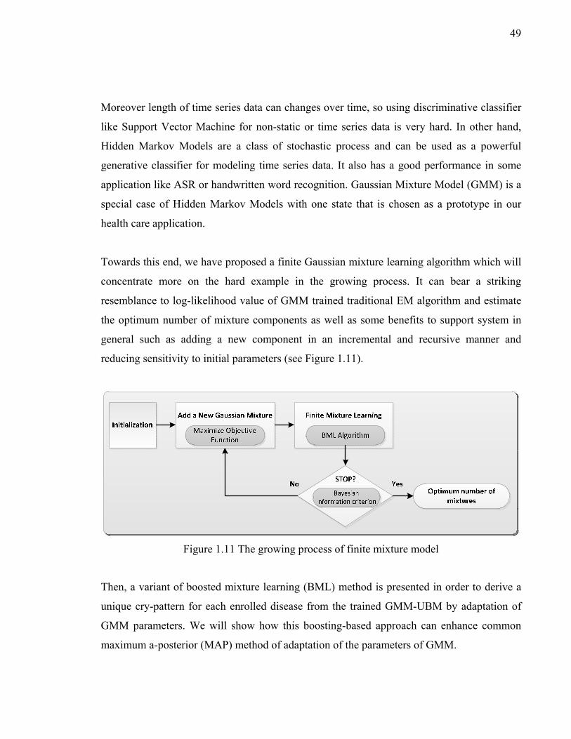
49
Moreover length of time series data can changes over time, so using discriminative classifier
like Support Vector Machine for non-static or time series data is very hard. In other hand,
Hidden Markov Models are a class of stochastic process and can be used as a powerful
generative classifier for modeling time series data. It also has a good performance in some
application like ASR or handwritten word recognition. Gaussian Mixture Model (GMM) is a
special case of Hidden Markov Models with one state that is chosen as a prototype in our
health care application.
Towards this end, we have proposed a finite Gaussian mixture learning algorithm which will
concentrate more on the hard example in the growing process. It can bear a striking
resemblance to log-likelihood value of GMM trained traditional EM algorithm and estimate
the optimum number of mixture components as well as some benefits to support system in
general such as adding a new component in an incremental and recursive manner and
reducing sensitivity to initial parameters (see Figure 1.11).
Figure 1.11 The growing process of finite mixture model
Then, a variant of boosted mixture learning (BML) method is presented in order to derive a
unique cry-pattern for each enrolled disease from the trained GMM-UBM by adaptation of
GMM parameters. We will show how this boosting-based approach can enhance common
maximum a-posterior (MAP) method of adaptation of the parameters of GMM.
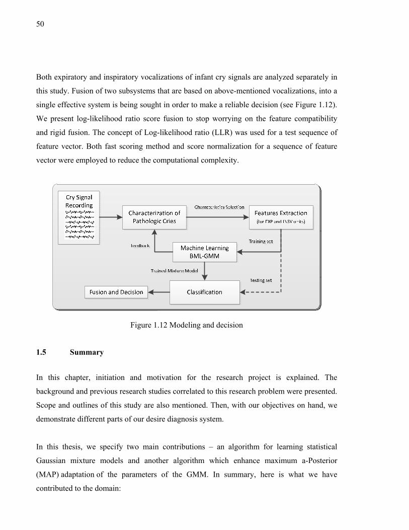
50
Both expiratory and inspiratory vocalizations of infant cry signals are analyzed separately in
this study. Fusion of two subsystems that are based on above-mentioned vocalizations, into a
single effective system is being sought in order to make a reliable decision (see Figure 1.12).
We present log-likelihood ratio score fusion to stop worrying on the feature compatibility
and rigid fusion. The concept of Log-likelihood ratio (LLR) was used for a test sequence of
feature vector. Both fast scoring method and score normalization for a sequence of feature
vector were employed to reduce the computational complexity.
Figure 1.12 Modeling and decision
1.5 Summary
In this chapter, initiation and motivation for the research project is explained. The
background and previous research studies correlated to this research problem were presented.
Scope and outlines of this study are also mentioned. Then, with our objectives on hand, we
demonstrate different parts of our desire diagnosis system.
In this thesis, we specify two main contributions – an algorithm for learning statistical
Gaussian mixture models and another algorithm which enhance maximum a-Posterior
(MAP) adaptation of the parameters of the GMM. In summary, here is what we have
contributed to the domain:

51
1. A design and implementation of a non-invasive cry-based diagnostic tool using
computer acoustical analysis of newborn cries to detect enrolled medical conditions such
as heart defects and infections. It is implemented using MATLAB software;
2. A boosted mixture learning algorithm for learning if statistical Gaussian mixture models
- This pertains to finding optimal number of mixture component and Gaussian
parameters;
3. A boosting-based adaptation algorithm to derive the hypothesized health-condition
model by adapting the parameters of UBM;
4. Separate analysis of both expiratory and inspiratory cry vocalizations and employing
valuable information that comes from the fusion of the two independent subsystems in
decision making process;
5. Various experiments that demonstrate that our idea of proposed classification system is
possible and feasible. Moreover, it can be extended to represent more disease and
syndromes, providing enough corresponding infant cry data.

CHAPITRE 2
CRY-BASED CLASSIFICATION OF HEALTHY AND SICK INFANTS USING ADAPTED BOOSTED MIXTURE LEARNING METHOD FOR GAUSSIAN
MIXTURE MODELS
Hesam Farsaie Alaie, Chakib Tadj
Department of Electrical Engineering, École de Technologie Supérieure,
1100 Notre Dame West, Montréal, Québec, H3C 1K3, Canada
This article is published in “Journal of Modeling and Simulation in Engineering”, volume
2012 (2012), Article ID 983147, 10 pages, Accepted 30 November 2012
Résumé
Nous utilisons de l'information présente dans le signal cri des nourrissons afin de déterminer
l'état psychologique de l'enfant. Un mélange de gaussiennes (GMMs) est utilisé afin de
distinguer entre les nourrissons nés à termes en bonne santés, les prématurés, et ceux qui ont
des problèmes médicaux spécifiques. Des modèles de cri pour chaque état pathologique sont
créés en utilisant la méthode adapted boosted mixture learning (BML) pour estimer les
paramètres du modèle de mixture. Dans nos expériences, nous comparons la méthode
proposée à un système de référence utilisant un algorithme EM, pour Expectation-
Maximisation, pour la classification multi-pathologique. Les résultats des tests ont démontré
que la méthode BML adaptée pour l'apprentissage de GMM a une meilleure performance que
celle utilisant l’algorithme EM. Le system de diagnostic proposé, extrait des coefficients de
Fourier (MFCC) comme un vecteur de caractéristiques des modèles de cri des nouveau-nés.
Dans l'expérience de classification binaire, le système identifie le cri comme appartenant à
l'un des deux groupes, sains ou pathologique. Le classificateur binaire a réalisé un taux réel
positif de 80,77% et un taux réel négatif de 86,96%, ce qui montre la capacité du système à
identifier correctement les nourrissons en bonne santé et malades, respectivement.
54
2.1 Abstract
We make use of information inside infant’s cry signal in order to identify the infant’s
psychological condition. Gaussian mixture models (GMMs) are applied to distinguish
between healthy full-term and premature infants, and those with specific medical problems
available in our cry database. Cry pattern for each pathological condition is created by using
adapted boosted mixture learning (BML) method to estimate mixture model parameters. In
the first experiment, test results demonstrate that the introduced adapted BML method for
learning of GMMs has a better performance than conventional EM-based reestimation
algorithm as a reference system in multipathological classification task. This newborn cry-
based diagnostic system (NCDS) extracted Mel-frequency cepstral coefficients (MFCCs) as a
feature vector for cry patterns of newborn infants. In binary classification experiment, the
system discriminated a test infant’s cry signal into one of two groups, namely, healthy and
pathological based on MFCCs. The binary classifier achieved a true positive rate of 80.77%
and a true negative rate of 86.96% which show the ability of the system to correctly identify
healthy and diseased infants, respectively.
2.2 Introduction
Crying is the first sound the baby makes when he enters the world outside of his mother’s
womb, which is a very positive sign of a new healthy life. Infants cry for the same reason that
adults talk i.e. to let others know about their needs or problems. Since crying is all a baby can
do to express any discomfort, it seems that this multimodal signal carries a lot of information
about him. In early studies of the infant cry analysis, the acoustic structure of infant crying
was analyzed and some of the important variables controlling the production of their cries
were described (Wasz-Hockert, Michelsson et Lind, 1985). After cry analysis on infants with
various diseases, in some cases it has been noticed that there are fixed cry attributes, which
are rarely seen in cries of healthy infants. Instead, these attributes occur frequently in cries of
infants with diseases (Benson, 2009; Wasz-Hockert et al., 1968; Wasz-Hockert, Michelsson
et Lind, 1985). Therefore the concealed information contained within a cry signal could
clarify the infant’s present psychological condition. Acoustic analysis of the infants' cry
55
signal helps to measure these parameters quantitatively to perform a comparison between
healthy and ill states. Since infants’ cry could be changed from normal to abnormal by
diseases or deformities which have the ability to produce a ill effect on the central nervous
system, the oral cavities, or respiratory organs, our goal is to develop a NCDS to classify
infants with different kind of physiological conditions.
Generally, sounds can be represented in multiple ways. In feature representation method, the
features selection step relies heavily on good understanding of the problem. There are some
literatures on defining and using different cry characteristics and frequency features which
distinguish between a healthy infant’s cry and that of infants with asphyxia, brain damage,
Hyperbilirubinemia, Down’s syndrome, and mothers who were drug-abused abused during
pregnancy (Corwin, Lester et Golub, 1996; Wasz-Hockert, Michelsson et Lind, 1985).
Human speech features characteristics such as linear prediction coefficients (LPCs), MFCCs,
fundamental frequency and formants are studied in previous works (Amaro-Camargo et
Reyes-García, 2007; Benson, 2009; Cano et al., 2006; Galaviz et García, 2005; Lind et
Wermke, 2002; Orozco et Garcia, 2003). The work presented by Hariharan, et al, employed
wavelet packet transform (WPT) to compute sub-band energy and entropy features from
wavelet packet coefficients (Hariharan, Yaacob et Awang, 2011). The goal is given a set of
exemplary patterns for different pathological infant’s cry classes, to construct a function
such that when presented with a new feature from an infant’s cry belonging to class the
function will recognize the correct index pathology class. In recent years, several machine
learning algorithms such as artificial neural network (ANN), radial basis function (RBF),
probabilistic neural network (PNN) have demonstrated their ability to recognize cry patterns
and make intelligent decision based on available training database (Cano Ortiz, Escobedo
Beceiro et Ekkel, 2004a; Hariharan, Yaacob et Awang, 2011; Orozco et Garcia, 2003).
Furthermore, hybrid systems in which classification methods are combined under several
approaches like bagging (Bauer et Kohavi, 1999a), boosting (Bauer et Kohavi, 1999a),
majority voting, staking were examined in order to achieve better final results than the case
where a single classifier is run (Amaro-Camargo et Reyes-García, 2007; Cano et al., 2006;
Galaviz et García, 2005).

56
In this paper we make use of extracted MFCCs from an infant’s cry signal to diagnose
pathological conditions and specific diseases which have not been previously studied such as
“Coarctation of Aorta” and “Tetralogy of Fallot” by drawing support from collected cry
database. As we mentioned earlier, there exists a large number of approaches to do the
modeling and the classification tasks. We will focus on GMMs, which is the most successful
classifiers in use for audio data when their temporal structure is not important (Divakaran,
2009). This paper employs GMMs to introduce a classification technique in the field of
statistical learning theory which uses adapted BML method to train mixture models for
modeling of infants’ cry signals. The BML method (Jun, Yu et Hui, 2011) presents three key
advantages: (1) Add new components into the direction that largely increases the objective
function, (2) Decrease sensitivity to initial parameters and (3) Estimate the optimum number
of components, unlike the conventional EM-based re-estimation algorithm. Partial and global
updating methods were used in model parameters estimation processes in order to speed
learning process up and converge to more robust and reliable estimation of a new mixture
component. Another advantage of the adapted BML method was that it used Bayesian
Information Criterion (BIC) (Schwarz, 1978) for model selection. It is partially based on the
likelihood function but to avoid overfitting there is also a penalty term.
This paper is organized as follows: In section 2.3 we give a brief review of GMM, its role in
cry-pattern classifier, and advantages of adapted BML method. Section 2.4 explains the
different parts of the NCDS and how it identified infants. In section 2.5, results of
experiments in both multi-pathological and binary classification tasks are reported, and in
section 2.6 a follow up analysis of the results and conclusion are presented to finalize the
paper.
2.3 GMMs for Cry-Pattern Classification
GMMs are a special case of Hidden Markov Models (HMMs) which pay more attention to
the temporal structure of a sound and have proven to be invaluable tools in areas such as
speech recognition (Divakaran, 2009). Compared to the human speech which is modeled by
Hidden Markov Models with finite states, cry signal has just a single state to be considered.
57
Moreover, GMM has the ability to form smooth approximations from arbitrarily shaped
densities and it has proved to be an effective probabilistic model for applications such as
biometric systems, most notably in speaker recognition systems and speaker identification
(Reynolds et Rose, 1995) due to its capability of representing a large class of sample
distributions. In a cry-based diagnosis system there is no chance to train the classifier with a
specific individual compared to what happens in speaker dependent automatic speech
recognition (ASR) systems. Therefore we should use our available cry database to create a
more general model for each available pathological condition in order to fine tune the
pathology detection of test infants. Like ASR systems in learning phase, there are two main
parts(O’Shaughnessy, 2008): first, some cry features are selected and then patterns are
created from these features. Second, the cry-pattern classifier works according to the just
created cry-patterns to recognize physiological conditions on the newborn infants. The
proposed cry-modeling method trained the GMM classifier from feature streams. It means
that cry signals coming from either healthy or pathological classes were modeled by a
separate pool of Gaussians using extracted feature vectors. Adapted BML was used to learn
mixture models in an incremental and recursive manner in which unlike EM-based re-
estimation algorithm, the final model was less sensitive to initial parameters. It might,
therefore, converge to a better optimal point. According to the boosting theory, upper bound
on training error rate is analytically minimized and the margin of all training samples is
increased. Moreover, in the preceding paper (Jun, Yu et Hui, 2011) the strong point of BML
method shows that a new Gaussian component is estimated in each step according to the
functional gradient of the objective function. Therefore each new component is always added
to the direction that increases the objective function the most. In this paper adapted BML has
been described for the log-likelihood function of the mixture model over training data as our
objective function.

58
2.4 Newborn Cry-Based Diagnosis System (NCDS)
2.4.1 Cry Database
The number of labeled data used during training phase has a leading role in performance of
the classifier. For example in case of having small number of cry samples for the pathologies
of interest, the resulting trained classifier may be too specific to be generalized to unseen
infant’s cry signal. Cry database collecting is still in progress and up to now, the following
two kinds of newborn infants are considered in the database:
1- Healthy newborn infants, both full-term and premature;
2- Sick newborn infants, both full-term and premature, with specific selected pathologies.
The imbalanced learning problem (He, 2011) is concerned with the performance of learning
algorithms. In the presence of underrepresented data and skewed class distribution this
problem arises, which is direct result of the nature of the data space present in the cry
database. Table 2.1 shows the list of different pathologies and the number of available
samples in each class.
2.4.2 Pre-processing and feature extraction
In data collection step we have used 2-channel recorder with 44.1 kHz sampling rate. The
time domain representation of one cry signal in two channels is shown in Figure 2.1. In pre-
processing step it converted into one channel signal using mean value function.
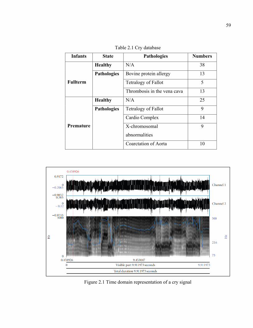
59
Table 2.1 Cry database
Infants State Pathologies Numbers
Fullterm
Healthy N/A 38
Pathologies Bovine protein allergy 13
Tetralogy of Fallot 5
Thrombosis in the vena cava 13
Premature
Healthy N/A 25
Pathologies Tetralogy of Fallot 9
Cardio Complex 14
X-chromosomal
abnormalities
9
Coarctation of Aorta 10
Figure 2.1 Time domain representation of a cry signal
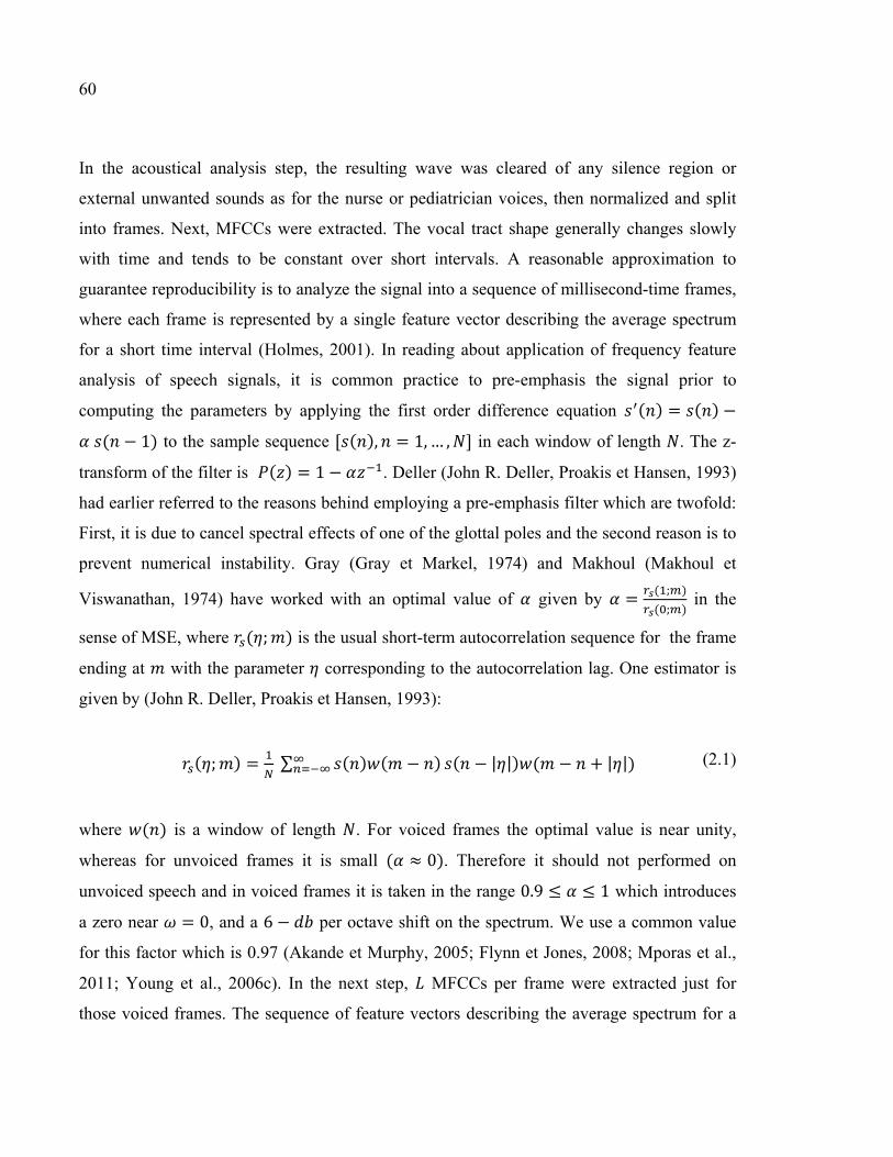
60
In the acoustical analysis step, the resulting wave was cleared of any silence region or
external unwanted sounds as for the nurse or pediatrician voices, then normalized and split
into frames. Next, MFCCs were extracted. The vocal tract shape generally changes slowly
with time and tends to be constant over short intervals. A reasonable approximation to
guarantee reproducibility is to analyze the signal into a sequence of millisecond-time frames,
where each frame is represented by a single feature vector describing the average spectrum
for a short time interval (Holmes, 2001). In reading about application of frequency feature
analysis of speech signals, it is common practice to pre-emphasis the signal prior to
computing the parameters by applying the first order difference equation ( ) = ( ) − ( − 1) to the sample sequence [ ( ), = 1,… , ] in each window of length . The z-
transform of the filter is ( ) = 1 − . Deller (John R. Deller, Proakis et Hansen, 1993)
had earlier referred to the reasons behind employing a pre-emphasis filter which are twofold:
First, it is due to cancel spectral effects of one of the glottal poles and the second reason is to
prevent numerical instability. Gray (Gray et Markel, 1974) and Makhoul (Makhoul et
Viswanathan, 1974) have worked with an optimal value of given by = ( ; )( ; ) in the
sense of MSE, where ( ; ) is the usual short-term autocorrelation sequence for the frame
ending at with the parameter corresponding to the autocorrelation lag. One estimator is
given by (John R. Deller, Proakis et Hansen, 1993):
( ; ) = ∑ ( ) ( − ) ( − | |) ( − + | |) (2.1)
where ( ) is a window of length . For voiced frames the optimal value is near unity,
whereas for unvoiced frames it is small ( ≈ 0). Therefore it should not performed on
unvoiced speech and in voiced frames it is taken in the range 0.9 ≤ ≤ 1 which introduces
a zero near = 0, and a 6 − per octave shift on the spectrum. We use a common value
for this factor which is 0.97 (Akande et Murphy, 2005; Flynn et Jones, 2008; Mporas et al.,
2011; Young et al., 2006c). In the next step, MFCCs per frame were extracted just for
those voiced frames. The sequence of feature vectors describing the average spectrum for a

61
short time interval can be presented as a matrix which acts like a pattern in the classification
phase.
In all related practical applications, the short terms or frames should be utilized which
implies that the signal characteristics are uniform in the region. Therefore the selected
portion of the signal has to be short enough to be stationary. Temporal properties can be
assumed fixed over time intervals on the order of 10-30 msec (Rabiner et Schafer, 1978).
Prior to any frequency analysis, the Hamming windowing is necessary to reduce any
discontinuities at the edges of the selected region. Generally a longer window will tend to
produce a better spectral picture of the signal while the window is completely within a
stationary region, whereas a shorter window will tend to resolve events in the signal better in
time. This trade-off is sometimes called the spectral temporal resolution trade-off (John R.
Deller, Proakis et Hansen, 1993). A common choice for the value of the window length (10-
30 msec) (Benzeghiba et al., 2007; Huang, Acero et Hon, 2001a; O’Shaughnessy, 2008;
Rabiner et Schafer, 1978) is normally larger than the frame rate. For example, the typical
values for the window length in HTK (Young et al., 2006c) is 25ms. MFCCs are obtained by
applying the Discrete Cosine Transform (DCT) to the output of the Mel-filters. The
difference from the real cepstrum is that a nonlinear frequency scale is used, which
approximates the behavior of the auditory system (Rabiner et Schafer, 1978). A filterbank
with filter is defined, where all these triangular filters compute the average spectrum
around each center frequency with increasing bandwidth. An acoustic representation using
MFCCs is often referred as a “mel cepstrum”. After performing fast Fourier Transform (FFT)
on each windowed frame, MFCCs are calculated using the following DCT (Divakaran,
2009):
= ∑ × cos − ⁄ , = 1,2,… (2.2)
where K is the number of sub-bands, is the desired length of cepstrum and , =1,2, … (1 ≤ ≤ ), represents the filter bank energy after passing through the triangular
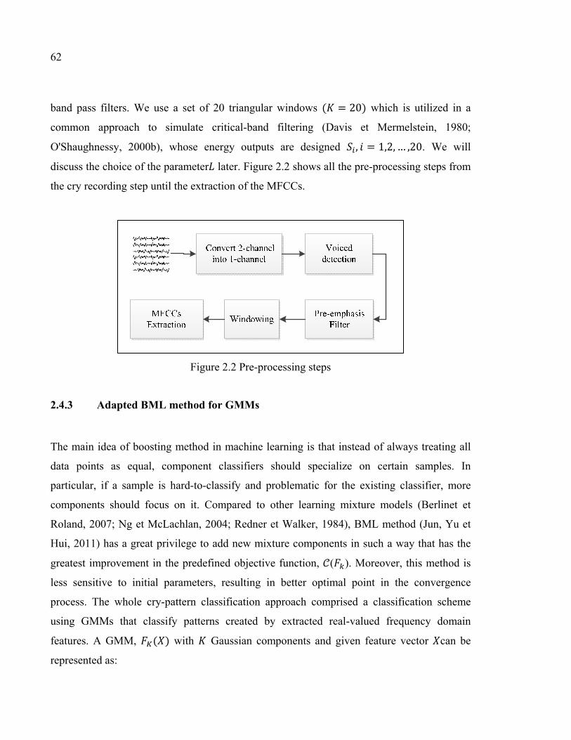
62
band pass filters. We use a set of 20 triangular windows ( = 20) which is utilized in a
common approach to simulate critical-band filtering (Davis et Mermelstein, 1980;
O'Shaughnessy, 2000b), whose energy outputs are designed , = 1,2, … ,20. We will
discuss the choice of the parameter later. Figure 2.2 shows all the pre-processing steps from
the cry recording step until the extraction of the MFCCs.
Figure 2.2 Pre-processing steps
2.4.3 Adapted BML method for GMMs
The main idea of boosting method in machine learning is that instead of always treating all
data points as equal, component classifiers should specialize on certain samples. In
particular, if a sample is hard-to-classify and problematic for the existing classifier, more
components should focus on it. Compared to other learning mixture models (Berlinet et
Roland, 2007; Ng et McLachlan, 2004; Redner et Walker, 1984), BML method (Jun, Yu et
Hui, 2011) has a great privilege to add new mixture components in such a way that has the
greatest improvement in the predefined objective function, ( ). Moreover, this method is
less sensitive to initial parameters, resulting in better optimal point in the convergence
process. The whole cry-pattern classification approach comprised a classification scheme
using GMMs that classify patterns created by extracted real-valued frequency domain
features. A GMM, ( ) with Gaussian components and given feature vector can be
represented as:
63
( ) = ∑ ( ) (2.3)
with the restriction that 0 ≤ ≤ 1 for = 1,… , and
∑ = 1 (2.4)
where and ( ) are mixture proportions and distributions of the component
respectively. The multivariate Gaussian component of a D-dimensional feature vector
can be written in the following notation:
( | ) = ( ; , )= 1(2 ) | | × −12 ( − ) ( − )
(2.5)
where = [ , ] are the mean and covariance parameters for the component and
represents the transpose of matrix . The model commences with one mixture and
learns gradually by adding a new mixture component on each step. According to the defined
objective function (. ), each adding component process should satisfy the inequality ( ) > ( ).All the re-estimation formulas to update Gaussian distribution parameters
can be computed afterwards. Log-likelihood function of the mixture model over all training
feature data has a vital role in aforementioned formulas. For example, the pre-defined
objective function of the mixture model over all training feature can be computed using
equation below:
= ∑ ( ) (2.6)
where is the number of training feature vectors in pathology class. Iterative re-
estimation formulas for model parameters ( ) = [ , ]at the ( + 1) iteration
can be evaluated as follows:
64
( ) = ( )( | ) (2.7)
= ∑ ( ).∑ ( ) = ∑ ( ) .
(2.8)
= ∑ ( ) × ∑ ( )( − )( − ) (2.9)
where ( ) = [ , ] denotes the mean vector and covariance matrix for Gaussian
component at the iteration, and = [ , ]. Note how ( ) represents a weight
assigned to feature vector after iteration. As you can see according to this weighting
function it is clear to understand that feature vector with lower probability by current model
are given larger weights than those with more probability. Therefore, the new Gaussian
component focuses on those features which are poorly modeled by the current model
, in much the same way as other boosting algorithms (Freund et Schapire, 1997;
Friedman, 2001).
2.4.4 Initialization of sample weights
There is a problem with the initialization values of weights based on boosting theory which
can be computed by using equation below:
( ) = 1 ( | )⁄ (2.10)
where = [ , ]. The dynamic range of is large in a way that it could be
dominated by only a few number of samples with low probability or outliers. We use the so-
called ‘Weight decay’ method (Rosset, 2005) to overcompensate for the low probability by
smoothing sample weights based on power scaling.
( ) = (1 ( | ))⁄ , 0 < < 1 (2.11)
65
where is a decay parameter or an exponential scaling factor. In the second method the idea
of sampling boosting in (Freund et Schapire, 1997) is applied to form a subset of training
feature vectors according to the mean and variance values of the decayed weights.
Afterwards, vectors contained in the just created subset are utilized with equal weights to
estimate the new component parameters. Assume Μ and denote the mean and variance of
weights calculated in Equation (10) as defined below:
= [ ( )] (2.12)
= [ ( )] (2.13)
Then, the aforementioned subset with large weights is selected as described below:
= | [ ( )] > + (2.14)
where is a linear scaling factor to control the size of subset .
2.4.5 Process of adding a new component
In the adding process the part of training vectors in which ( ) had a higher value than the
reminder of the mixture model, denoted by − [ ], was selected. Then this subset of data
should be modeled by a small GMM consisting in two Gaussian components called ∗ and .The initial component came from the EM-based re-estimation, and then the second
component and its weight were estimated based on BML method and line search
respectively. We considered the estimated component –the second one– as an initial
component and ran BML method again. This process continues repeatedly, until it reached
the optimal maximum log-likelihood estimate of parameters over . This procedure for
finding the best two new components and ∗ continued for = 1,… , . Amongst all
the created mixture models, denoted by , the one that gave the highest value of the
objective function (same as log-likelihood value) was selected and added to the mixture by
adjusting its weight.

66
2.4.6 Partial and global updating
During previous step, instead of finding the new mixture weight from the line search below:
∗ = ∈[ , ] (1 − ) + ∗ (2.15)
There is an alternative method called partial updating in which each new component and its
weight are estimated at the same time, which is preferable since it may result in more robust
and reliable estimation.
∗, ∗ = ,, ( (1 − ) + ) (2.16)
All the equations for updating weight assigned to feature vector , mixture weight value,
mean and covariance matrix are estimated as follows (Jun, Yu et Hui, 2011):
( ) = ( )( ) + (1 − ) ( | )
(2.17)
( ) = ( )∑ ( )
(2.18)
= 1 ( )
(2.19)
= ( ) .
(2.20)
= ( ) . ( − ) × ( − )
(2.21)

67
Moreover, in order to speed converging process up and finding the minimum number of
Gaussian component in the final mixture, current mixture model should be updated
globally over training data samples before adding the next component. For example in the
GMM with components, denoted by , the component can be re-estimated for = 1,… , when the reminder of the mixture mode is assumed to be fixed. This procedure
continues iteratively until the objective function value reaches a local maximum. It means
that after obtaining a mixture model , we could update each component and its weight
over all training feature vectors by using the same updating equations.
2.4.7 Criterion for model selection
The process of adding new mixture component to previous mixture model continued
incrementally and recursively until the optimal number of mixtures is met. The set of
Gaussian components selected should represent the space covered by the feature vectors. For
this purpose the selected strategy to stop the adding process is a criterion-based called
Bayesian Information Criterion (BIC). It can be represented as the following (Schwarz,
1978):
( ) = −2 × ( ) + (2.22)
where ( ) is the log-likelihood function of the mixture model over all training data, is
the number of parameters used in model , and denotes total number of training data for
the pathology class. The second term in BIC equation is a penalty term for the number of
parameters in the model. BIC is closely related to Akaike Information Criterion (AIC)
(Akaike, 1974; Bengtsson et Cavanaugh, 2006) but the penalty term is larger in BIC than in
AIC. Figure 2.3 shows brief review of all mentioned processes to train a GMM for each
available pathological condition in order.
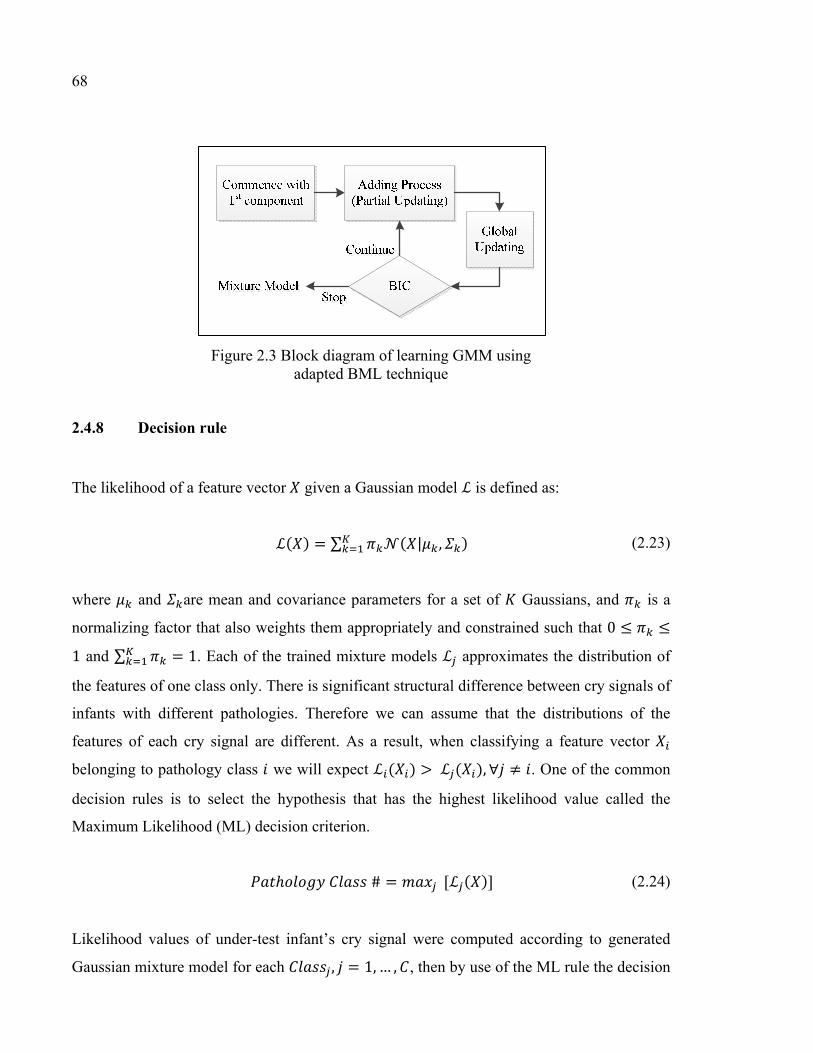
68
Figure 2.3 Block diagram of learning GMM using adapted BML technique
2.4.8 Decision rule
The likelihood of a feature vector given a Gaussian model ℒ is defined as:
ℒ( ) = ∑ ( | , ) (2.23)
where and are mean and covariance parameters for a set of Gaussians, and is a
normalizing factor that also weights them appropriately and constrained such that 0 ≤ ≤1 and ∑ = 1. Each of the trained mixture models ℒ approximates the distribution of
the features of one class only. There is significant structural difference between cry signals of
infants with different pathologies. Therefore we can assume that the distributions of the
features of each cry signal are different. As a result, when classifying a feature vector
belonging to pathology class we will expect ℒ ( ) > ℒ ( ), ∀ ≠ . One of the common
decision rules is to select the hypothesis that has the highest likelihood value called the
Maximum Likelihood (ML) decision criterion.
ℎ # = [ℒ ( )] (2.24)
Likelihood values of under-test infant’s cry signal were computed according to generated
Gaussian mixture model for each , = 1,… , , then by use of the ML rule the decision
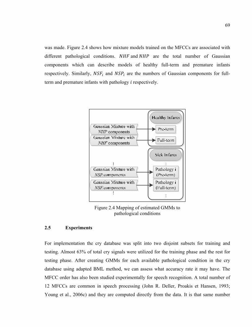
69
was made. Figure 2.4 shows how mixture models trained on the MFCCs are associated with
different pathological conditions. and are the total number of Gaussian
components which can describe models of healthy full-term and premature infants
respectively. Similarly, and are the numbers of Gaussian components for full-
term and premature infants with pathology respectively.
Figure 2.4 Mapping of estimated GMMs to pathological conditions
2.5 Experiments
For implementation the cry database was split into two disjoint subsets for training and
testing. Almost 63% of total cry signals were utilized for the training phase and the rest for
testing phase. After creating GMMs for each available pathological condition in the cry
database using adapted BML method, we can assess what accuracy rate it may have. The
MFCC order has also been studied experimentally for speech recognition. A total number of
12 MFCCs are common in speech processing (John R. Deller, Proakis et Hansen, 1993;
Young et al., 2006c) and they are computed directly from the data. It is that same number
NSPi
NSFi
70
which is used in (Nwe, Foo et De Silva, 2003) to recognize speech emotion via HMMs. The
energy within a frame is also an important feature that can be easily obtained. For better
performance, the 0 cepstral coefficient [ ] is appended to the feature vector as the 13rd
feature. The initial coefficient represents the average energy (weighting with a zero-
frequency cosine) same as role of the log energy [ = ∑ ]a (Huang, Acero et Hon,
2001b; O'Shaughnessy, 2000a). Therefore, used feature vectors are composed of first 13
MFCCs [ , = 0,1,2,… , = 12]. As we defined earlier, is the desired length of cepstrum
and it is a fixed parameter. The higher-order MFCC does not further reduce the relative error
rate with a typical speech recognition system in comparison with the 13th-order MFCC,
which indicates that the first 13 coefficients already contain most salient information needed
for speech recognition (Huang, Acero et Hon, 2001a). We made full use of both initialization
methods with decay parameter = 0.05 and linear scaling factor = −0.5 values for the
parameters to overcome overfitting and the small covariance matrix which was created after
several iterations. It is those same parameter values which are set and designed for BML
algorithm in large-vocabulary continuous speech recognition tasks in (Jun, Yu et Hui, 2011).
After that only samples in subset with equal sample weights were used to estimate the mean
and covariance matrix of Gaussian components. The presented method had a vital role to
achieve good performance and avoid the overfitting problem in the learning step.
In the first experiment, the NCDS was tested on several multi-pathology classification tasks.
It consisted of all aforementioned conditions in the cry database. It could be difficult to
evaluate the effectiveness of the created GMMs for modeling and adapted BML method for
learning the mixture model by extracting a single feature from a small cry database.
Nevertheless our results show that it had a better accuracy rate compared with conventional
EM-based method for GMMs as our reference system. It is worth mentioning that the GMMs
created by the EM-based re-estimation method for each class were trained by setting the
number of components equal to that of mixture model learned by adapted BML method.
Here, we address the question of the classification performance with respect to the frame
length by evaluating the system with different frame durations but same overlap percentages
(30%) between two consecutive windows. In order to extract MFCCs, frames with different
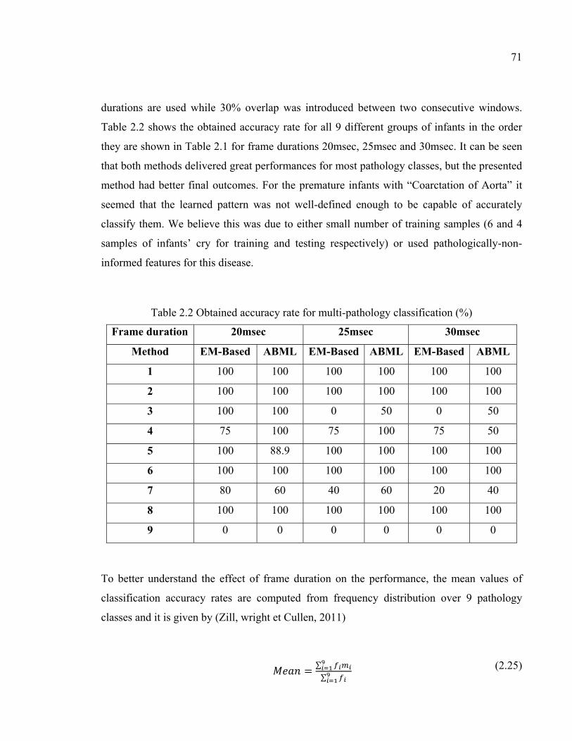
71
durations are used while 30% overlap was introduced between two consecutive windows.
Table 2.2 shows the obtained accuracy rate for all 9 different groups of infants in the order
they are shown in Table 2.1 for frame durations 20msec, 25msec and 30msec. It can be seen
that both methods delivered great performances for most pathology classes, but the presented
method had better final outcomes. For the premature infants with “Coarctation of Aorta” it
seemed that the learned pattern was not well-defined enough to be capable of accurately
classify them. We believe this was due to either small number of training samples (6 and 4
samples of infants’ cry for training and testing respectively) or used pathologically-non-
informed features for this disease.
Table 2.2 Obtained accuracy rate for multi-pathology classification (%)
Frame duration 20msec 25msec 30msec
Method EM-Based ABML EM-Based ABML EM-Based ABML
1 100 100 100 100 100 100
2 100 100 100 100 100 100
3 100 100 0 50 0 50
4 75 100 75 100 75 50
5 100 88.9 100 100 100 100
6 100 100 100 100 100 100
7 80 60 40 60 20 40
8 100 100 100 100 100 100
9 0 0 0 0 0 0
To better understand the effect of frame duration on the performance, the mean values of
classification accuracy rates are computed from frequency distribution over 9 pathology
classes and it is given by (Zill, wright et Cullen, 2011)
= ∑∑ (2.25)
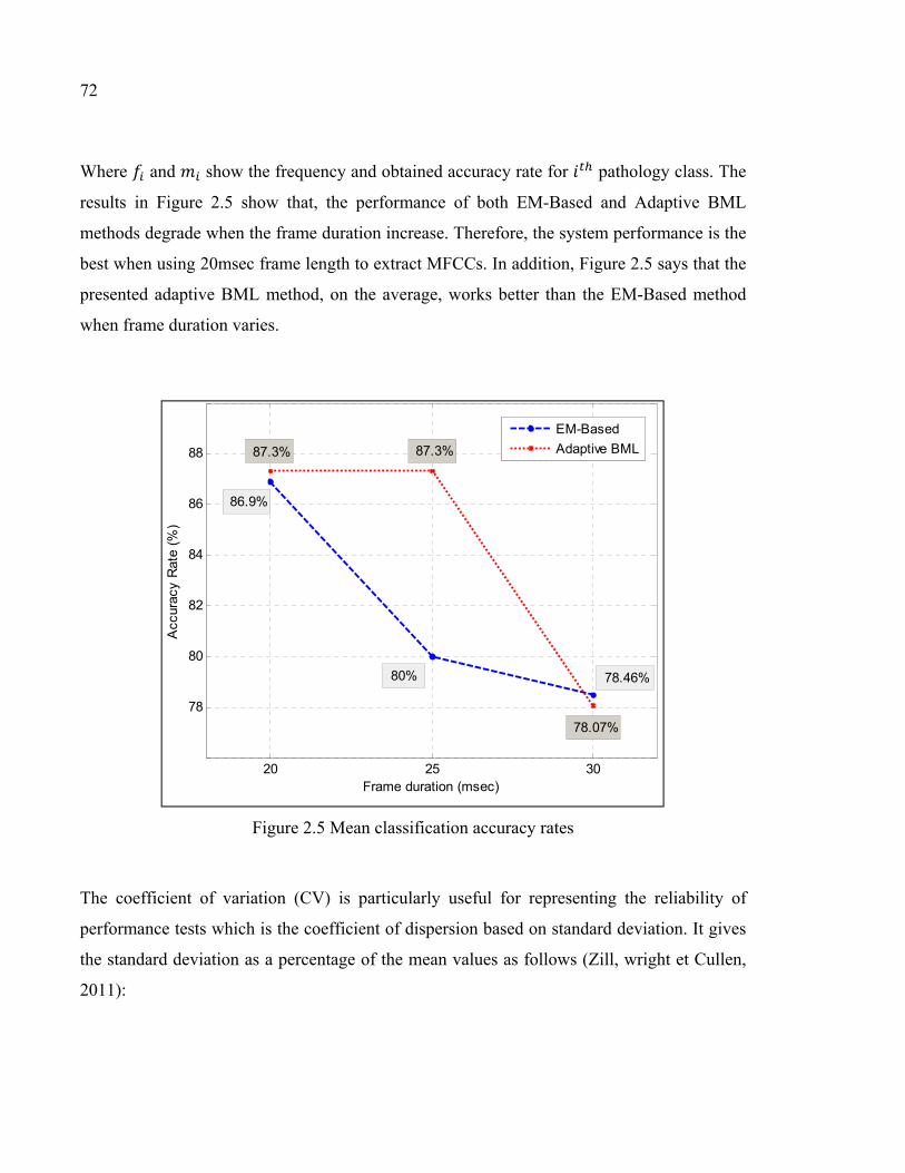
72
Where and show the frequency and obtained accuracy rate for pathology class. The
results in Figure 2.5 show that, the performance of both EM-Based and Adaptive BML
methods degrade when the frame duration increase. Therefore, the system performance is the
best when using 20msec frame length to extract MFCCs. In addition, Figure 2.5 says that the
presented adaptive BML method, on the average, works better than the EM-Based method
when frame duration varies.
Figure 2.5 Mean classification accuracy rates
The coefficient of variation (CV) is particularly useful for representing the reliability of
performance tests which is the coefficient of dispersion based on standard deviation. It gives
the standard deviation as a percentage of the mean values as follows (Zill, wright et Cullen,
2011):
20 25 30
78
80
82
84
86
88
Frame duration (msec)
Acc
urac
y R
ate
(%)
EM-Based
Adaptive BML87.3% 87.3%
86.9%
80%
78.07%
78.46%
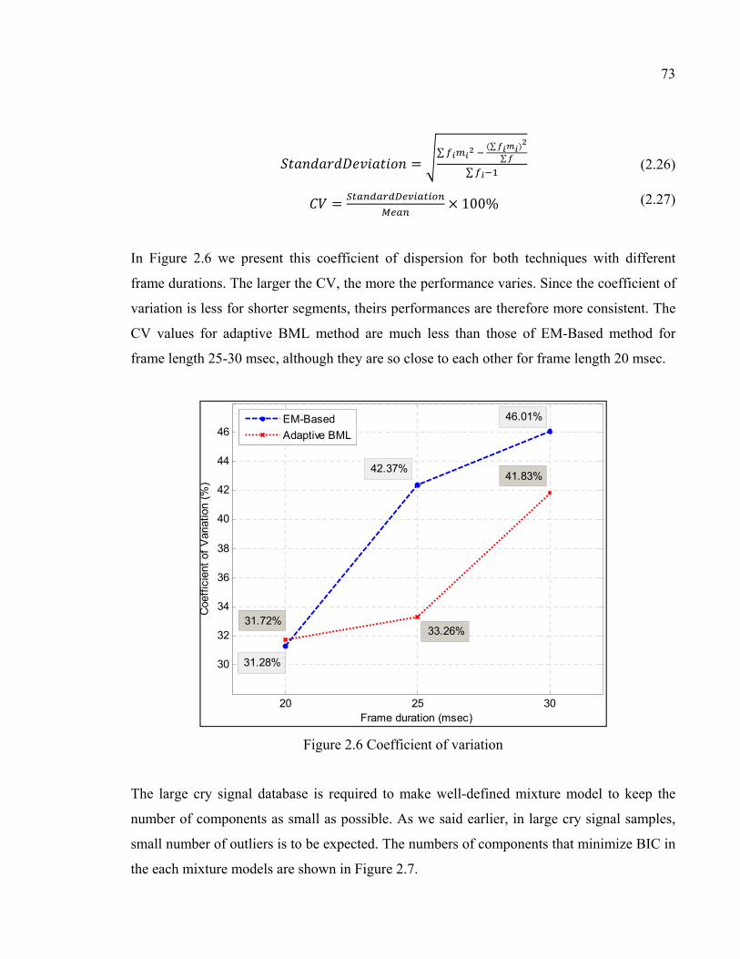
73
= ∑ (∑ )∑∑ (2.26)
= × 100% (2.27)
In Figure 2.6 we present this coefficient of dispersion for both techniques with different
frame durations. The larger the CV, the more the performance varies. Since the coefficient of
variation is less for shorter segments, theirs performances are therefore more consistent. The
CV values for adaptive BML method are much less than those of EM-Based method for
frame length 25-30 msec, although they are so close to each other for frame length 20 msec.
Figure 2.6 Coefficient of variation
The large cry signal database is required to make well-defined mixture model to keep the
number of components as small as possible. As we said earlier, in large cry signal samples,
small number of outliers is to be expected. The numbers of components that minimize BIC in
the each mixture models are shown in Figure 2.7.
20 25 30
30
32
34
36
38
40
42
44
46
Frame duration (msec)
Coe
ffic
ient
of
Var
iatio
n (%
)
EM-Based
Adaptive BML
31.28%
31.72%33.26%
42.37%41.83%
46.01%
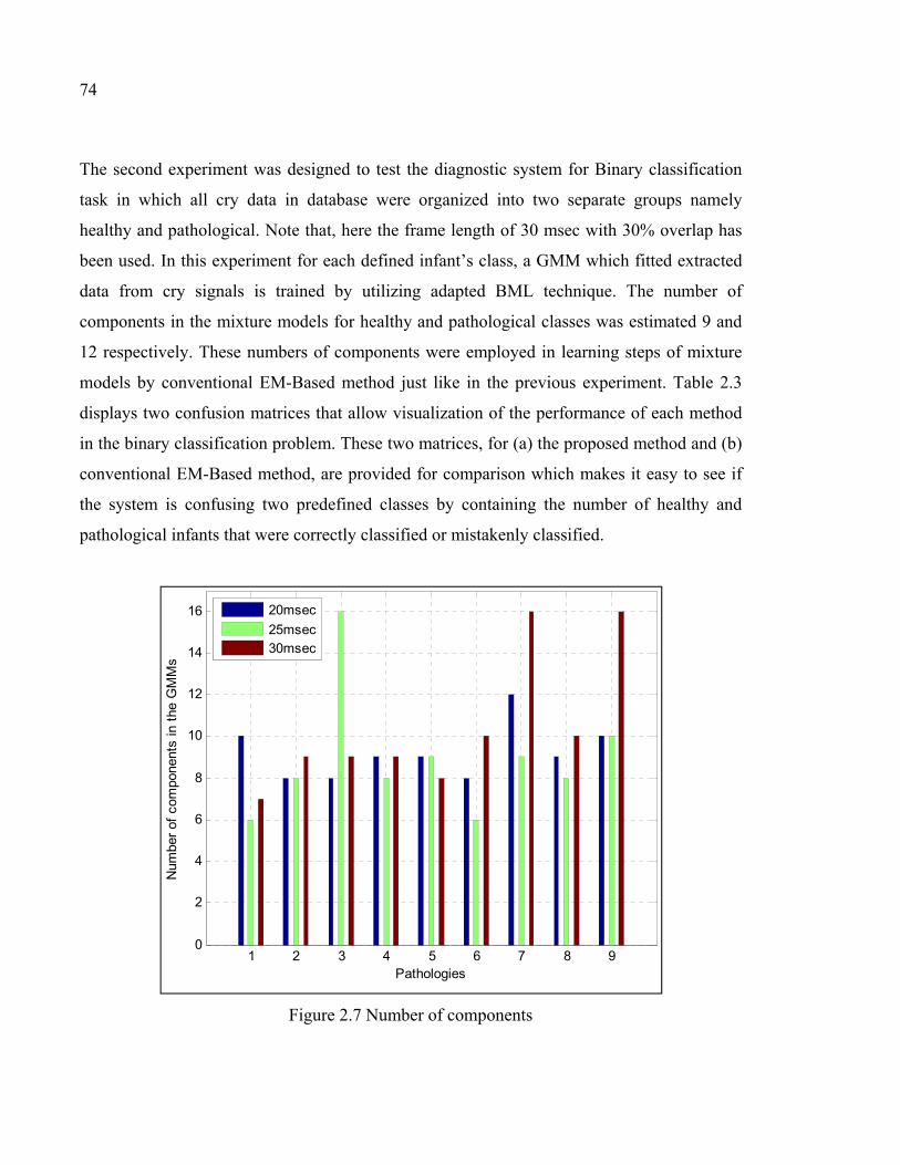
74
The second experiment was designed to test the diagnostic system for Binary classification
task in which all cry data in database were organized into two separate groups namely
healthy and pathological. Note that, here the frame length of 30 msec with 30% overlap has
been used. In this experiment for each defined infant’s class, a GMM which fitted extracted
data from cry signals is trained by utilizing adapted BML technique. The number of
components in the mixture models for healthy and pathological classes was estimated 9 and
12 respectively. These numbers of components were employed in learning steps of mixture
models by conventional EM-Based method just like in the previous experiment. Table 2.3
displays two confusion matrices that allow visualization of the performance of each method
in the binary classification problem. These two matrices, for (a) the proposed method and (b)
conventional EM-Based method, are provided for comparison which makes it easy to see if
the system is confusing two predefined classes by containing the number of healthy and
pathological infants that were correctly classified or mistakenly classified.
Figure 2.7 Number of components
1 2 3 4 5 6 7 8 90
2
4
6
8
10
12
14
16
Pathologies
Num
ber
of c
ompo
nent
s in
the
GM
Ms
20msec
25msec30msec

75
Table 2.3 Confusion Matrix for defined Binary classification task
Predicted Classes
Actual Classes Pathological Healthy
Pathological 21 5
Healthy 3 20
(a) Proposed ABML-GMM method
Predicted Classes
Actual Classes Pathological Healthy
Pathological 26 0
Healthy 6 17
(b) Conventional EM-GMM method
True positive (TP) and True negative (TN) rates are defined for a two by two confusion
matrix, as calculated using the following equations (Kohavi et Provost, 1998):
= + (2.28)
= + (2.29)
where “a” and “d” are the numbers of correct predictions that an instance is negative or
positive respectively. The other parameters, “b” and “c” are defined in a similar way by
counting the number of incorrect predictions that an instance is positive or negative
accordingly. In the pathology diagnostics system, true positive rate or test sensitivity shows
the ability of the system to correctly detect infants with disease, whereas true negative rate or
test specificity demonstrate the ability of the system to correctly identify those without
disease. Both these statistical measures of the two methods are summarized in Table 2.4.
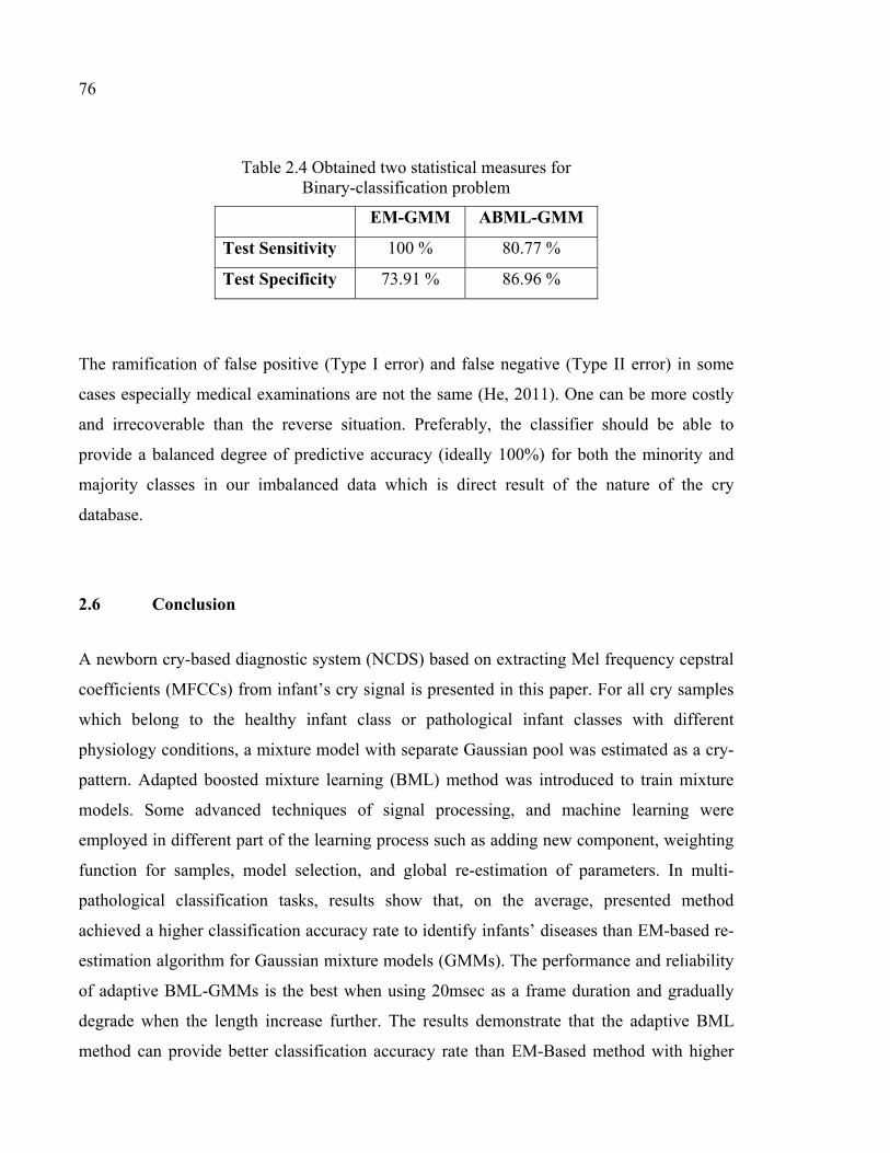
76
Table 2.4 Obtained two statistical measures for Binary-classification problem
EM-GMM ABML-GMM
Test Sensitivity 100 % 80.77 %
Test Specificity 73.91 % 86.96 %
The ramification of false positive (Type I error) and false negative (Type II error) in some
cases especially medical examinations are not the same (He, 2011). One can be more costly
and irrecoverable than the reverse situation. Preferably, the classifier should be able to
provide a balanced degree of predictive accuracy (ideally 100%) for both the minority and
majority classes in our imbalanced data which is direct result of the nature of the cry
database.
2.6 Conclusion
A newborn cry-based diagnostic system (NCDS) based on extracting Mel frequency cepstral
coefficients (MFCCs) from infant’s cry signal is presented in this paper. For all cry samples
which belong to the healthy infant class or pathological infant classes with different
physiology conditions, a mixture model with separate Gaussian pool was estimated as a cry-
pattern. Adapted boosted mixture learning (BML) method was introduced to train mixture
models. Some advanced techniques of signal processing, and machine learning were
employed in different part of the learning process such as adding new component, weighting
function for samples, model selection, and global re-estimation of parameters. In multi-
pathological classification tasks, results show that, on the average, presented method
achieved a higher classification accuracy rate to identify infants’ diseases than EM-based re-
estimation algorithm for Gaussian mixture models (GMMs). The performance and reliability
of adaptive BML-GMMs is the best when using 20msec as a frame duration and gradually
degrade when the length increase further. The results demonstrate that the adaptive BML
method can provide better classification accuracy rate than EM-Based method with higher

77
system reliability. For binary classification problem, with 30msec frame duration (the worst-
case scenario), adapted BML can identify full-term and pre-mature healthy infants better than
EM-Based, but on the other hand it deliver a little lower performance than EM-Based method
for sick infants. However, adapted BML provides better balanced degree of predictive
accuracy for both the minority and majority classes (test sensitivity 80.77% and test
specificity 86.96%).
2.7 Acknowledgment
We would like to thank Dr. Barrington and members of neonatology group of Mother and
Child University Hospital Center in Montreal (QC) for their dedication of the collection of
the Infant's cry data base. This research work has been funded by a grant from the Bill &
Melinda Gates Foundation through the Grand Challenges Explorations Initiative.

CHAPITRE 3
SPLITTING OF GAUSSIAN MODELS VIA ADAPTED BML METHOD
PERTAINING TO CRY-BASED DIAGNOSTIC SYSTEM
Hesam Farsaie Alaie, Chakib Tadj
Department of Electrical Engineering, École de Technologie Supérieure,
1100 Notre Dame West, Montréal, Québec, H3C 1K3, Canada
This article is published in “Journal of Engineering”, volume 5, Pages 277-283
Received June 2013
Résumé
Dans cet article, nous utilisons la méthode boosting afin d'introduire un nouvel algorithme
d'apprentissage pour GMM (Gaussian Mixture Models), appelé adapted Boosted Mixture
Learning (BML). La méthode possède la capacité de corriger les problèmes existants dans
d'autres techniques classiques pour estimer les paramètres GMM, due en partie à une
nouvelle stratégie de mélange pour augmenter le nombre de gaussiennes. L'idée de la
séparation discriminatoire est employée pour des densités de mélange de gaussiennes. Celle-
ci est suivie par une étape d’apprentissage selon la méthode proposée. Ensuite, le
classificateur de GMM est appliqué afin de différencier entre les nourrissons en bonne santé
et ceux qui présentent une des pathologies étudiées. Chacun des deux groupes comprend à la
fois des bébés prématurés et à terme. Chaque état pathologique est représenté par un modèle
créé en utilisant la méthode adaptée BML et des vecteurs de 13 coefficients MFCC. Les
résultats des tests démontrent que la méthode proposée pour entrainer les GGM a une
meilleure performance que le système de référence utilisant un algorithme EM, (Expectation-
Maximisation) pour la classification multi-pathologique.
80
3.1 Abstract
In this paper we make use of the boosting method to introduce a new learning algorithm for
Gaussian Mixture Models (GMMs) called adapted Boosted Mixture Learning (BML). The
method possesses the ability to rectify the existing problems in other conventional techniques
for estimating the GMM parameters, due in part to a new mixing-up strategy to increase the
number of Gaussian components. The discriminative splitting idea is employed for Gaussian
mixture densities followed by learning via introduced method. Then, the GMM classifier was
applied to distinguish between healthy infants and those that present a selected set of medical
conditions. Each group includes both full-term and premature infants. Cry-pattern for each
pathological condition is created by using the adapted BML method and 13-dimensional
Mel-Frequency Cepstral Coefficients (MFCCs) feature vector. The test results demonstrate
that the introduced method for training GMMs has a better performance than the traditional
method based upon random splitting and EM-based re-estimation as a reference system in
multi-pathological classification task.
Keywords: Adapted Boosted Mixture Learning; Gaussian Mixture Model; Splitting of
Gaussians; Expected-Maximization Algorithm, Cry Signals.
3.2 Introduction
Gaussian Mixture Model (GMM) has the capability to form smooth approximations to
arbitrarily shaped densities and it has proved to be an effective probabilistic model for
biometric systems, most notably in speaker recognition systems and speaker identification
(Reynolds et Rose, 1995). The GMMs are estimated from available training data using a
special case of the Expectation-Maximization (EM) algorithm based on the maximum-
likelihood (ML) (Dempster, Laird et Rubin, 1977).A finite amount of sample data produces
detrimental effects that commit statistical errors in training of the GMMs. Nevertheless, this
iterative algorithm comes with a guarantee that there will be no decreasing in likelihood
81
function after each iteration and therefore converges to locally optimal parameters (Heck et
Chou, 1994). Performance degradation due to parameter estimation errors is a function of the
number of free parameters in the classifier (Heck et Chou, 1994), so there are still some
problems when increasing model complexity. For example, in Automatic Speech
Recognition (ASR) systems using HTK with the method based on random splitting and EM-
based re-estimation (Jun, Yu et Hui, 2011): First, there is no guarantee that the newly added
mixture from random splitting always increases the likelihood function prior to re-estimation.
Second, convergence to the optimum point in EM-based re-estimation is not guaranteed due
to the sensitivity to initial parameters of the randomly split Gaussians. More recently, the
traditional boosting method has been used to solve some problems of mixture models (Kim et
Pavlovic, 2007; Pavlovic, 2004). Another new method called Boosted Mixture Learning
(BML) to learn Gaussian mixture Hidden Markov Model (HMM) is introduced to overcome
the aforementioned problems in other available conventional techniques for estimating the
GMM parameters (Jun, Yu et Hui, 2011). In (Boyu et al., 2010) the discriminative splitting
idea has been used for log-linear mixture densities in a speech recognition task. For this
purpose, the parameters of Gaussian model have been transformed into their equivalents in
log-linear model as presented in (Heigold et al., 2011; Heigold et al., 2008), and then trained
in a Maximum Mutual Information (MMI) framework.
GMMs represent a statistical pattern recognition approach that enables optimal processing of
data both for training (EM algorithm) the classifier and performing on-line classification.
Cry-based diagnostic system for newborn infants can be valuable in medical problems which
are currently undetectable until it is too late for treatment. Recently several classifiers such as
General Regression Neural Network (GRNN), Multi-Layer Perceptron (MLP), Time Delay
Neural Network (TDNN), Probabilistic Neural Network (PNN), Radial Basis Function (RBF)
and hybrid systems under several approaches such as bagging and boosting (Bauer et Kohavi,
1999b) were examined for discriminating between normal and sick infant’s cry signals
(Amaro-Camargo et Reyes-García, 2007; Cano et al., 2006; Galaviz et García, 2005;
Hariharan, Sindhu et Yaacob, 2012; Hariharan, Yaacob et Awang, 2011; Orozco et Garcia,
2003; Ortiz, Beceiro et Ekkel, 2004). In our previous work (Farsaie Alaie et Tadj, 2012), we
82
made use of cry signals to distinguish between healthy and sick infants both full-term and
premature. Most of the previous studies (Amaro-Camargo et Reyes-García, 2007; Cano et al.,
2006; Galaviz et García, 2005; Hariharan, Sindhu et Yaacob, 2012; Hariharan, Yaacob et
Awang, 2011; Orozco et Garcia, 2003; Ortiz, Beceiro et Ekkel, 2004; Wasz-Hockert,
Michelsson et Lind, 1985) concentrate on health status of infants via a binary classification
task, but this paper focuses on identifying several different pathological conditions. In this
article a method for splitting of Gaussian mixture densities is presented based on the boosting
algorithm to maximize the frame-level ML objective function. The performed experiments
on the diagnosis of infants’ diseases show that it has fairly superior performance to the
conventional method based on random splitting and EM-based re-estimation.
This paper is organized as follows: In section 3.3 we give a brief review of GMM. Section
3.4 explains the different parts of introduced learning algorithm. In section 3.5, preprocessing
steps and experiments are reported, and in section 3.6 a follow-up analysis of the results and
a conclusion are presented at the end to finalize this paper.
3.3 Gaussian mixture model
A complete GMM for a dimensional continuous value data vector called can be
represented by the weighted sum of Gaussian component densities = [ , , Σ ] = 1,… , as follows:
( | ) = ∑ ( ; , Σ ) , ∑ = 1 (3.1)
where each mixture component is a −dimensional multivariate Gaussian distribution
and , , Σ are the mixture weights, mean vector and covariance matrix respectively. Since
GMMs are used usually in unsupervised learning and clustering problems with unknown
number of mixtures and their parameters, the choice of model configuration is almost
determined by the amount of data available for estimating the GMM parameters in a
particular application. GMM, as a parametric probability density function with the following

83
adapted learning method could be a successful candidate for cry-based physical or
psychological status identification system.
3.4 Adapted boosted mixture model
Generally, boosting method combines weak learners or base classifiers in a weighted
majority voting scheme to improve the overall classification accuracy for almost any type of
learning algorithm (Bishop, 2006; Duda, Hart et Stork, 2001). The main idea of boosting is
that instead of always treating all data points as equal, component classifiers should
specialize on certain examples. Moreover, some recent work has shown that the boosting
method can effectively increase the margin of all training samples, which can be explained
by a theoretical view related to functional gradient techniques (Jun, Yu et Hui, 2011). We
should note that the boosting algorithm does not always improve the accuracy of a learning
algorithm nor does it always increase the margin.
In the presented method a new component and its weight can be trained based
discriminatively based on a predefined objective function, denoted as , in an optimal way.
Then, they will be added to the previous mixture model which has − 1 mixture
components to grow into a new mixture model .
( ) = (1 − ) ( ) + ( ) (3.2)
Objective function is defined as the log likelihood function of the mixture model kF , based
on all training data [ , , … , ].
( ) = ∑ log ( ) (3.3)
where is a weight to combine the new mixture component with the current model. When a
new mixture component is added, it will increase the ML objective function with respect
to until the criterion which will be explained later is met.
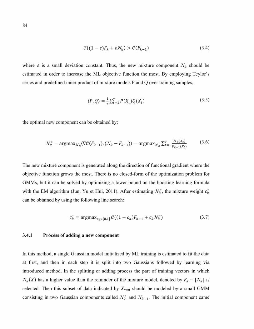
84
((1 − ) + ) > ( ) (3.4)
where is a small deviation constant. Thus, the new mixture component should be
estimated in order to increase the ML objective function the most. By employing Teylor’s
series and predefined inner product of mixture models P and Q over training samples,
⟨ , ⟩ = ∑ ( ) ( ) (3.5)
the optimal new component can be obtained by:
∗ = argmax ⟨∇ ( ), ( − )⟩ = argmax ∑ ( )( ) (3.6)
The new mixture component is generated along the direction of functional gradient where the
objective function grows the most. There is no closed-form of the optimization problem for
GMMs, but it can be solved by optimizing a lower bound on the boosting learning formula
with the EM algorithm (Jun, Yu et Hui, 2011). After estimating ∗, the mixture weight ∗ can be obtained by using the following line search:
∗ = argmax ∈[ , ] ((1 − ) + ∗) (3.7)
3.4.1 Process of adding a new component
In this method, a single Gaussian model initialized by ML training is estimated to fit the data
at first, and then in each step it is split into two Gaussians followed by learning via
introduced method. In the splitting or adding process the part of training vectors in which ( ) has a higher value than the reminder of the mixture model, denoted by − [ ] is
selected. Then this subset of data indicated by should be modeled by a small GMM
consisting in two Gaussian components called ∗ and . The initial component came

85
from the EM-based re-estimation, and then the second component and its weight were
estimated based upon adapted BML method. We considered the estimated component – the
second one – as an initial component and run the algorithm again. This process continues
repeatedly, until it reached the optimal maximum log-likelihood estimate of parameters over
. This procedure for finding the best two new components and ∗ continued for = 1,… , . Amongst all the created mixture models, denoted by , the one that gave
the highest value of the objective function was selected and added to the mixture by adjusting
its weight. This iterative density splitting process in ML framework is repeated as long as the
added component causes an increase in the predefined objective function.
3.4.2 Partial and global updating
During previous step, instead of finding the new mixture weight from the line search, there is
an alternative method called partial updating in which each new component and its weight
are estimated at the same time, which is preferable since it may result in more robust and
reliable estimation.
∗, ∗ = ,, ( (1 − ) + ) (3.8)
The iterative re-estimation formula for model parameters ( ) = [ , ] at the ( + 1) iteration can be evaluated as follows (Jun, Yu et Hui, 2011):
( ) = ( )( ) + (1 − ) ( | ) (3.9)
( ) = ( )∑ ( ) (3.10)
= 1 ( ) (3.11)

86
= ( ) . (3.12)
= ( ) . ( − ) × ( − ) (3.13)
where ( ) denotes the weight assigned to sample at the iteration, similar to
sample weights used in the traditional boosting algorithms and = [ , ]. Moreover,
in order to speed up converging process and finding the minimum number of Gaussian
component in the final mixture, the current mixture model should be updated globally
over training data samples before adding the next component. For example in the GMM with
components, denoted by , the component can be re-estimated for = 1,… , when
the reminder of the mixture mode is assumed to be fixed. It means that after obtaining a
mixture model , we could update each component and its weight over all training
feature vectors by using the same updating equations. The parameters updating phase,
subsequent to splitting the selected density in half, brings about an increase in the objective
function through the localized training of each component separately.
3.4.3 Initialization of sample weights
A problem may arise when the initial values of the weights are chosen by boosting theory as
follow:
( ) = 1 ( | )⁄ (3.14)
The dynamic range of is large in a way that it could be dominated by only a few number
of outliers or samples with low probabilities. We use the so-called ‘Weight decay’ method
(Rosset, 2005) to overcompensate for the low probability by smoothing sample weights
based on power scaling.
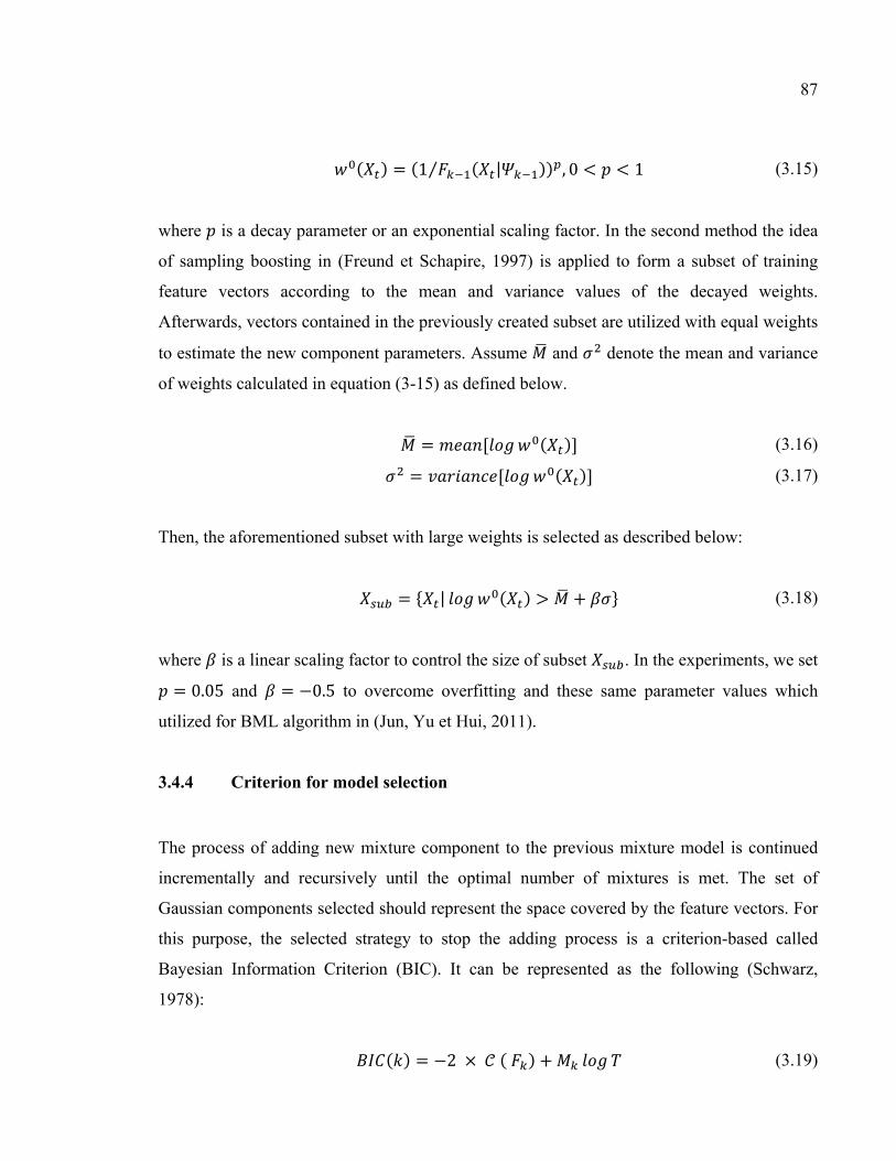
87
( ) = (1 ( | )⁄ ) , 0 < < 1 (3.15)
where is a decay parameter or an exponential scaling factor. In the second method the idea
of sampling boosting in (Freund et Schapire, 1997) is applied to form a subset of training
feature vectors according to the mean and variance values of the decayed weights.
Afterwards, vectors contained in the previously created subset are utilized with equal weights
to estimate the new component parameters. Assume and denote the mean and variance
of weights calculated in equation (3-15) as defined below.
= [ ( )] (3.16)
= [ ( )] (3.17)
Then, the aforementioned subset with large weights is selected as described below:
= | ( ) > + (3.18)
where is a linear scaling factor to control the size of subset . In the experiments, we set = 0.05 and = −0.5 to overcome overfitting and these same parameter values which
utilized for BML algorithm in (Jun, Yu et Hui, 2011).
3.4.4 Criterion for model selection
The process of adding new mixture component to the previous mixture model is continued
incrementally and recursively until the optimal number of mixtures is met. The set of
Gaussian components selected should represent the space covered by the feature vectors. For
this purpose, the selected strategy to stop the adding process is a criterion-based called
Bayesian Information Criterion (BIC). It can be represented as the following (Schwarz,
1978):
( ) = −2 × ( ) + (3.19)
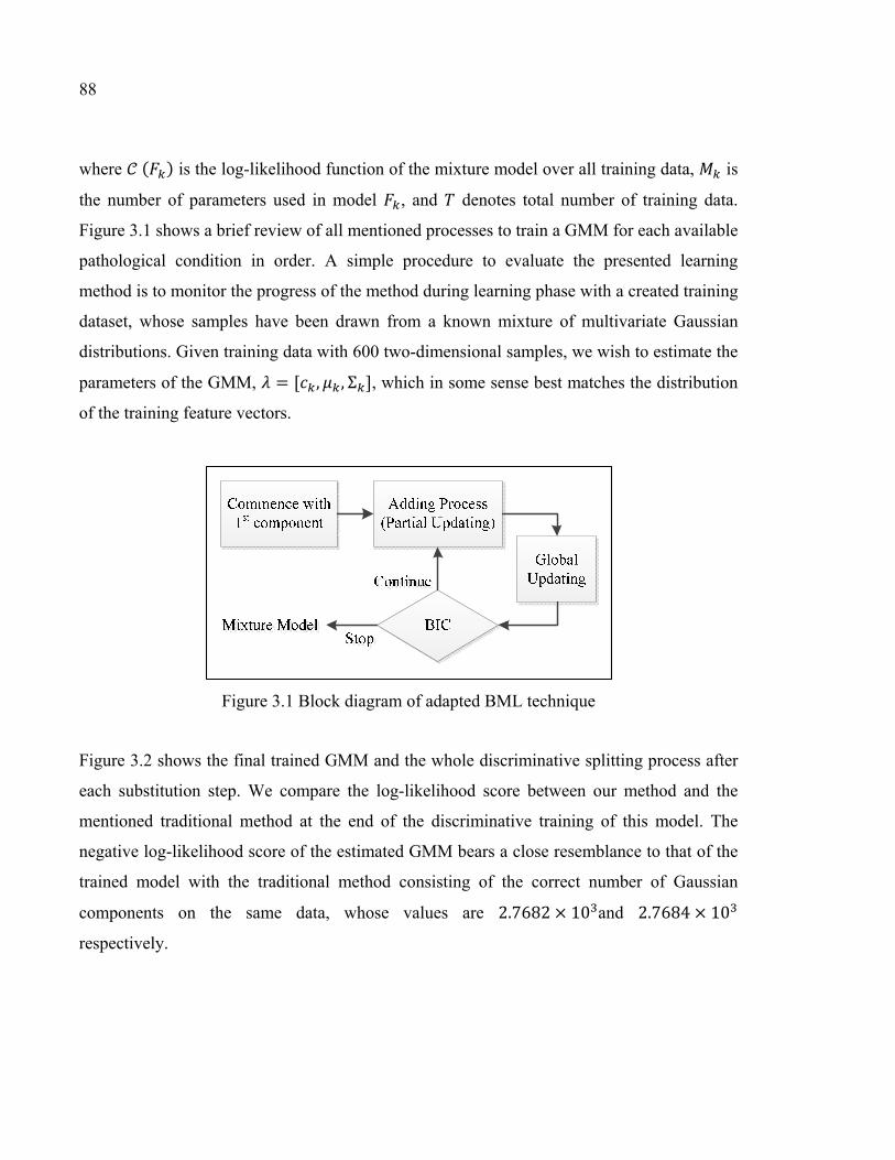
88
where ( ) is the log-likelihood function of the mixture model over all training data, is
the number of parameters used in model , and denotes total number of training data.
Figure 3.1 shows a brief review of all mentioned processes to train a GMM for each available
pathological condition in order. A simple procedure to evaluate the presented learning
method is to monitor the progress of the method during learning phase with a created training
dataset, whose samples have been drawn from a known mixture of multivariate Gaussian
distributions. Given training data with 600 two-dimensional samples, we wish to estimate the
parameters of the GMM, = [ , , Σ ], which in some sense best matches the distribution
of the training feature vectors.
Figure 3.1 Block diagram of adapted BML technique
Figure 3.2 shows the final trained GMM and the whole discriminative splitting process after
each substitution step. We compare the log-likelihood score between our method and the
mentioned traditional method at the end of the discriminative training of this model. The
negative log-likelihood score of the estimated GMM bears a close resemblance to that of the
trained model with the traditional method consisting of the correct number of Gaussian
components on the same data, whose values are 2.7682 × 10 and 2.7684 × 10
respectively.
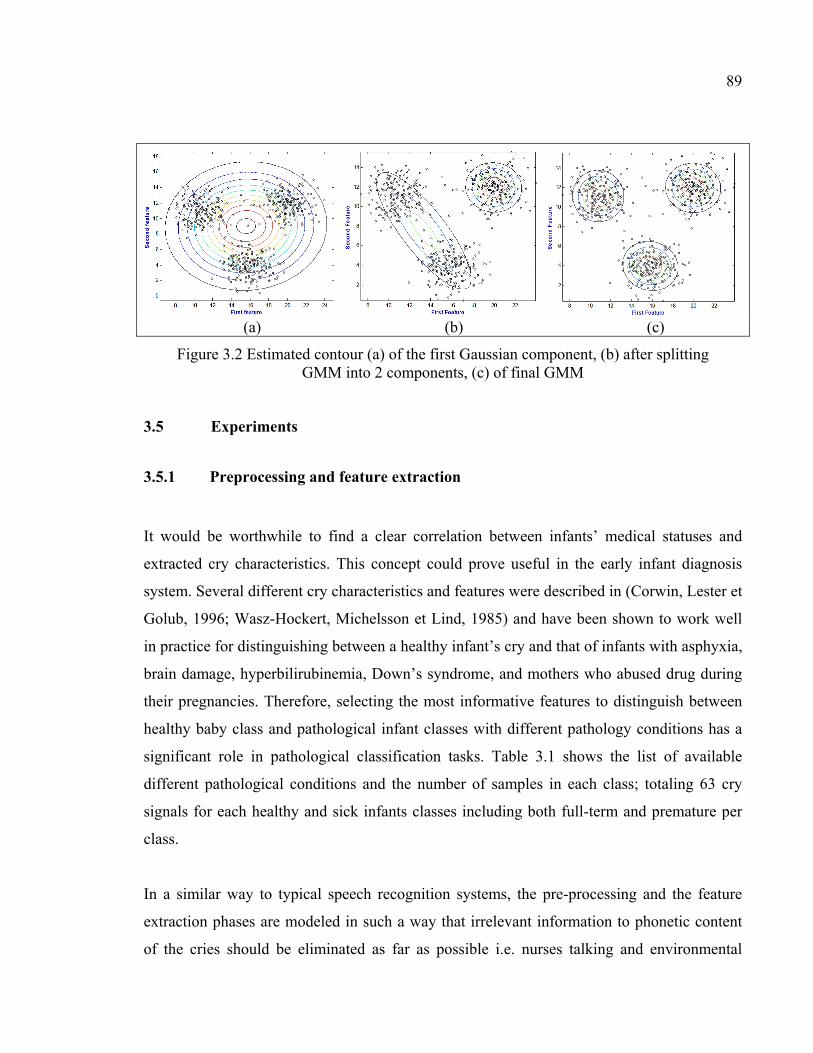
89
(a) (b) (c)
Figure 3.2 Estimated contour (a) of the first Gaussian component, (b) after splitting GMM into 2 components, (c) of final GMM
3.5 Experiments
3.5.1 Preprocessing and feature extraction
It would be worthwhile to find a clear correlation between infants’ medical statuses and
extracted cry characteristics. This concept could prove useful in the early infant diagnosis
system. Several different cry characteristics and features were described in (Corwin, Lester et
Golub, 1996; Wasz-Hockert, Michelsson et Lind, 1985) and have been shown to work well
in practice for distinguishing between a healthy infant’s cry and that of infants with asphyxia,
brain damage, hyperbilirubinemia, Down’s syndrome, and mothers who abused drug during
their pregnancies. Therefore, selecting the most informative features to distinguish between
healthy baby class and pathological infant classes with different pathology conditions has a
significant role in pathological classification tasks. Table 3.1 shows the list of available
different pathological conditions and the number of samples in each class; totaling 63 cry
signals for each healthy and sick infants classes including both full-term and premature per
class.
In a similar way to typical speech recognition systems, the pre-processing and the feature
extraction phases are modeled in such a way that irrelevant information to phonetic content
of the cries should be eliminated as far as possible i.e. nurses talking and environmental
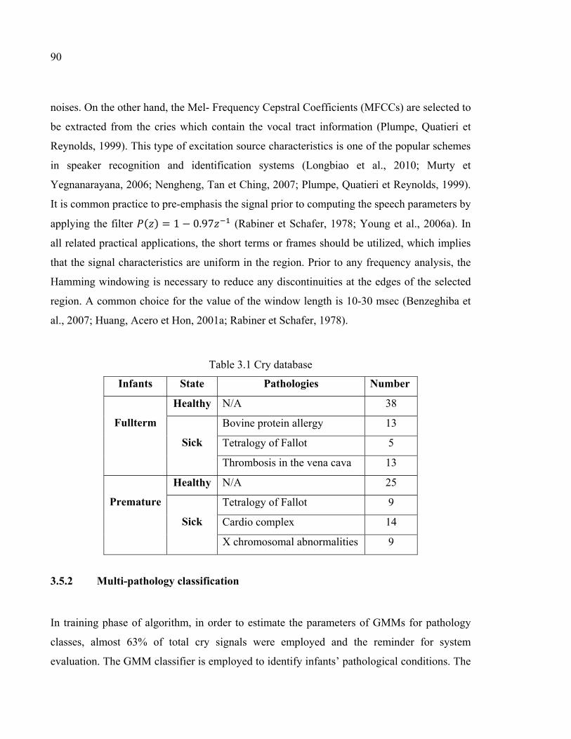
90
noises. On the other hand, the Mel- Frequency Cepstral Coefficients (MFCCs) are selected to
be extracted from the cries which contain the vocal tract information (Plumpe, Quatieri et
Reynolds, 1999). This type of excitation source characteristics is one of the popular schemes
in speaker recognition and identification systems (Longbiao et al., 2010; Murty et
Yegnanarayana, 2006; Nengheng, Tan et Ching, 2007; Plumpe, Quatieri et Reynolds, 1999).
It is common practice to pre-emphasis the signal prior to computing the speech parameters by
applying the filter ( ) = 1 − 0.97 (Rabiner et Schafer, 1978; Young et al., 2006a). In
all related practical applications, the short terms or frames should be utilized, which implies
that the signal characteristics are uniform in the region. Prior to any frequency analysis, the
Hamming windowing is necessary to reduce any discontinuities at the edges of the selected
region. A common choice for the value of the window length is 10-30 msec (Benzeghiba et
al., 2007; Huang, Acero et Hon, 2001a; Rabiner et Schafer, 1978).
Table 3.1 Cry database
Infants State Pathologies Number
Fullterm
Healthy N/A 38
Sick
Bovine protein allergy 13
Tetralogy of Fallot 5
Thrombosis in the vena cava 13
Premature
Healthy N/A 25
Sick
Tetralogy of Fallot 9
Cardio complex 14
X chromosomal abnormalities 9
3.5.2 Multi-pathology classification
In training phase of algorithm, in order to estimate the parameters of GMMs for pathology
classes, almost 63% of total cry signals were employed and the reminder for system
evaluation. The GMM classifier is employed to identify infants’ pathological conditions. The
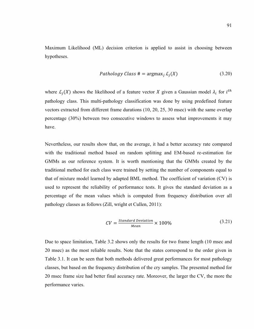
91
Maximum Likelihood (ML) decision criterion is applied to assist in choosing between
hypotheses.
ℎ # = argmax ℒ ( ) (3.20)
where ℒ ( ) shows the likelihood of a feature vector given a Gaussian model for
pathology class. This multi-pathology classification was done by using predefined feature
vectors extracted from different frame durations (10, 20, 25, 30 msec) with the same overlap
percentage (30%) between two consecutive windows to assess what improvements it may
have.
Nevertheless, our results show that, on the average, it had a better accuracy rate compared
with the traditional method based on random splitting and EM-based re-estimation for
GMMs as our reference system. It is worth mentioning that the GMMs created by the
traditional method for each class were trained by setting the number of components equal to
that of mixture model learned by adapted BML method. The coefficient of variation (CV) is
used to represent the reliability of performance tests. It gives the standard deviation as a
percentage of the mean values which is computed from frequency distribution over all
pathology classes as follows (Zill, wright et Cullen, 2011):
= × 100% (3.21)
Due to space limitation, Table 3.2 shows only the results for two frame length (10 msec and
20 msec) as the most reliable results. Note that the states correspond to the order given in
Table 3.1. It can be seen that both methods delivered great performances for most pathology
classes, but based on the frequency distribution of the cry samples. The presented method for
20 msec frame size had better final accuracy rate. Moreover, the larger the CV, the more the
performance varies.
92
Table 3.2 Obtained accuracy rate (%) for multi-pathology classification task
20 msec 10 msec
State EM-Based ABML EM-Based ABML
1 100 100 100 100
2 100 100 80 80
3 100 100 100 100
4 75 100 75 75
5 100 88.9 100 100
6 100 100 100 100
7 80 60 80 80
8 100 100 100 100
Mean 94.16 94.58 92.08 92.08
CV 10.9 12 11.8 11.8
3.6 Conclusion
An adapted mixture learning method for GMMs based on boosting algorithm is introduced in
this paper. Advanced techniques of signal processing, and machine learning were employed
in different parts of the learning process such as adding a new component per step, weighting
function for samples, model selection, and global re-estimation of parameters. The focus of
this paper has been on the application of discriminative training via introduced GMM-ABML
as it pertains to the pathology detection through infants’ cry signals. For each pathology class
in our cry database, the adapted BML method trained a mixture model with a separate
Gaussian pool as a cry-pattern. The results show that, on the average, it delivers a higher
classification accuracy rate (94.58%) than the traditional method based on random splitting
and EM-based re-estimation. It might be early to reach strong conclusions since there are not
enough cases of the pathological classes, but the results have the potential to serves as a
mixture learning method for further research. We are currently trying to use alternative

93
discriminative criteria like MMI rather than ML and collecting more sample cries for further
tests.
3.7 Acknowledgment
We would like to thank Dr. Barrington and members of neonatology group of Mother and
Child University Hospital Center in Montreal (QC) for their dedication of the collection of
the Infant's cry data base. This research work has been funded by a grant from the Bill &
Melinda Gates Foundation through the Grand Challenges Explorations Initiative.

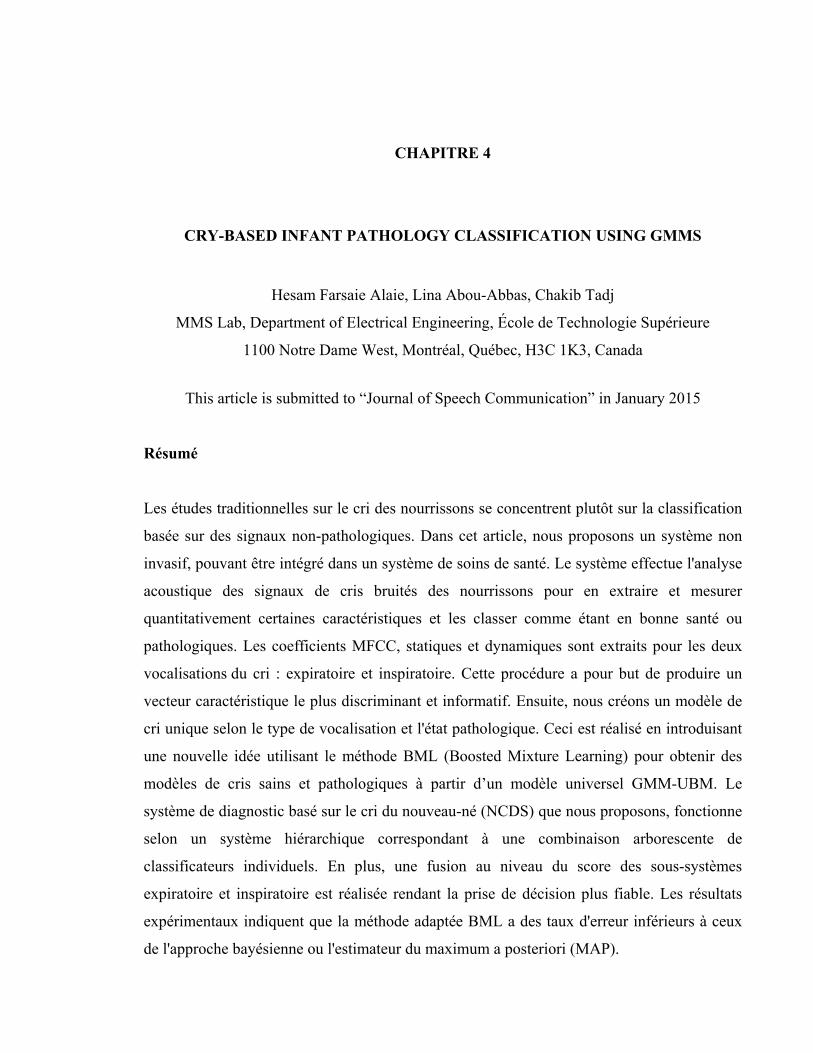
CHAPITRE 4
CRY-BASED INFANT PATHOLOGY CLASSIFICATION USING GMMS
Hesam Farsaie Alaie, Lina Abou-Abbas, Chakib Tadj
MMS Lab, Department of Electrical Engineering, École de Technologie Supérieure
1100 Notre Dame West, Montréal, Québec, H3C 1K3, Canada
This article is submitted to “Journal of Speech Communication” in January 2015
Résumé
Les études traditionnelles sur le cri des nourrissons se concentrent plutôt sur la classification
basée sur des signaux non-pathologiques. Dans cet article, nous proposons un système non
invasif, pouvant être intégré dans un système de soins de santé. Le système effectue l'analyse
acoustique des signaux de cris bruités des nourrissons pour en extraire et mesurer
quantitativement certaines caractéristiques et les classer comme étant en bonne santé ou
pathologiques. Les coefficients MFCC, statiques et dynamiques sont extraits pour les deux
vocalisations du cri : expiratoire et inspiratoire. Cette procédure a pour but de produire un
vecteur caractéristique le plus discriminant et informatif. Ensuite, nous créons un modèle de
cri unique selon le type de vocalisation et l'état pathologique. Ceci est réalisé en introduisant
une nouvelle idée utilisant le méthode BML (Boosted Mixture Learning) pour obtenir des
modèles de cris sains et pathologiques à partir d’un modèle universel GMM-UBM. Le
système de diagnostic basé sur le cri du nouveau-né (NCDS) que nous proposons, fonctionne
selon un système hiérarchique correspondant à une combinaison arborescente de
classificateurs individuels. En plus, une fusion au niveau du score des sous-systèmes
expiratoire et inspiratoire est réalisée rendant la prise de décision plus fiable. Les résultats
expérimentaux indiquent que la méthode adaptée BML a des taux d'erreur inférieurs à ceux
de l'approche bayésienne ou l'estimateur du maximum a posteriori (MAP).

96
Highlights • We characterize the distributions of the acoustic features of infant cry signals with
GMMs as a universal background model;
• An adapted BML method is presented to derive either healthy or pathology subclass
models from the GMM-UBM;
• A score level fusion of obtained log-likelihood ratio scores from both expiratory and
inspiratory sounds is performed;
• The proposed cry-based diagnostic system is used to classify healthy and sick infants;
• Subjective results indicated that the proposed method can perform better than Bayesian
adaptation.
4.1 Abstract
Traditional studies of infant cry signals focus more on non-pathology-based classification of
infants. In this article, we introduce a non-invasive health care system that performs acoustic
analysis of unclean noisy infants’ cry signals to extract and measure certain cry
characteristics quantitatively and classify healthy and sick newborn infants according to only
their cries. In the conduct of this newborn cry-based diagnostic system, the dynamic Mel-
Frequency Cepstral Coefficients (MFCC) features along with static MFCCs are selected and
extracted for both expiratory and inspiratory cry vocalizations to produce the most
discriminative and informative feature vector. Next, we create a unique cry pattern for each
cry vocalization type and pathological condition by introducing a novel idea using the
Boosted Mixture Learning (BML) method to derive either healthy or pathology subclass
models separately from the Gaussian Mixture Model-Universal Background Model (GMM-
UBM). Our newborn cry-based diagnostic system (NCDS) has a hierarchical scheme that is a
treelike combination of individual classifiers. Moreover, a score-level fusion of the proposed
expiratory and inspiratory cry-based subsystems is performed to make a reliable decision.
The experimental results indicate that the adapted BML method has lower error rates than the
Bayesian approach or the maximum a posteriori probability (MAP) adaptation approach
when considered as a reference method.
97
Keywords: Gaussian mixture model; Universal background model; Mel-frequency Cepstral
Coefficient; Likelihood ratio scores; Newborn infant cries; Expiratory sound; Inspiratory
sound.
4.2 Introduction
Crying is the first clear sign of life that is observed shortly after a baby’s live birth. Although
there have been some books and products that were created through the years to unlock the
secret language of babies, their potential for use in the early diagnosis and treatment of
newborns remains largely in an open and undeveloped state. The results of these
studies highlight the existence of some cry attributes in sick infants that are rarely observed
in the cries of healthy infants (Benson et Haith, 2009; Wasz-Hockert et al., 1968; Wasz-
Hockert, Michelsson et Lind, 1985). Instead, these attributes occur frequently in the cries of
sick infants who suffer from different medical diseases and conditions. Therefore, infant cry
characteristics reflect the integrity of the central nervous system.
4.2.1 Early studies and birth defects
Many early researchers defined several cry characteristics and presented their common
values, such as the fundamental frequency, formants, cry modes, cry latency, phonation,
hyperphonation, and dysphonation (LaGasse, Neal et Lester, 2005; Lederman, 2002;
Newman, 1985; Wasz-Hockert, Michelsson et Lind, 1985). Gradually, detailed acoustic
analysis, which measures and compares the acoustical characteristics of newborn infant cry
signals, shows hidden diagnostic potential of cry signals for the basic cry types and the cries
of infants in pathological conditions such as with brain damage, central nervous system
diseases and Down’s syndrome (Michelsson, 1971; Michelsson et Michelsson, 1999;
Partanen et al., 1967; Wasz-Hockert et al., 1968; Wasz-Hockert, Michelsson et Lind, 1985).
It appears that some of the symptoms are not always recognized or even do not appear for
months or years; thus, it might be too late for treatment after clinical symptoms start,
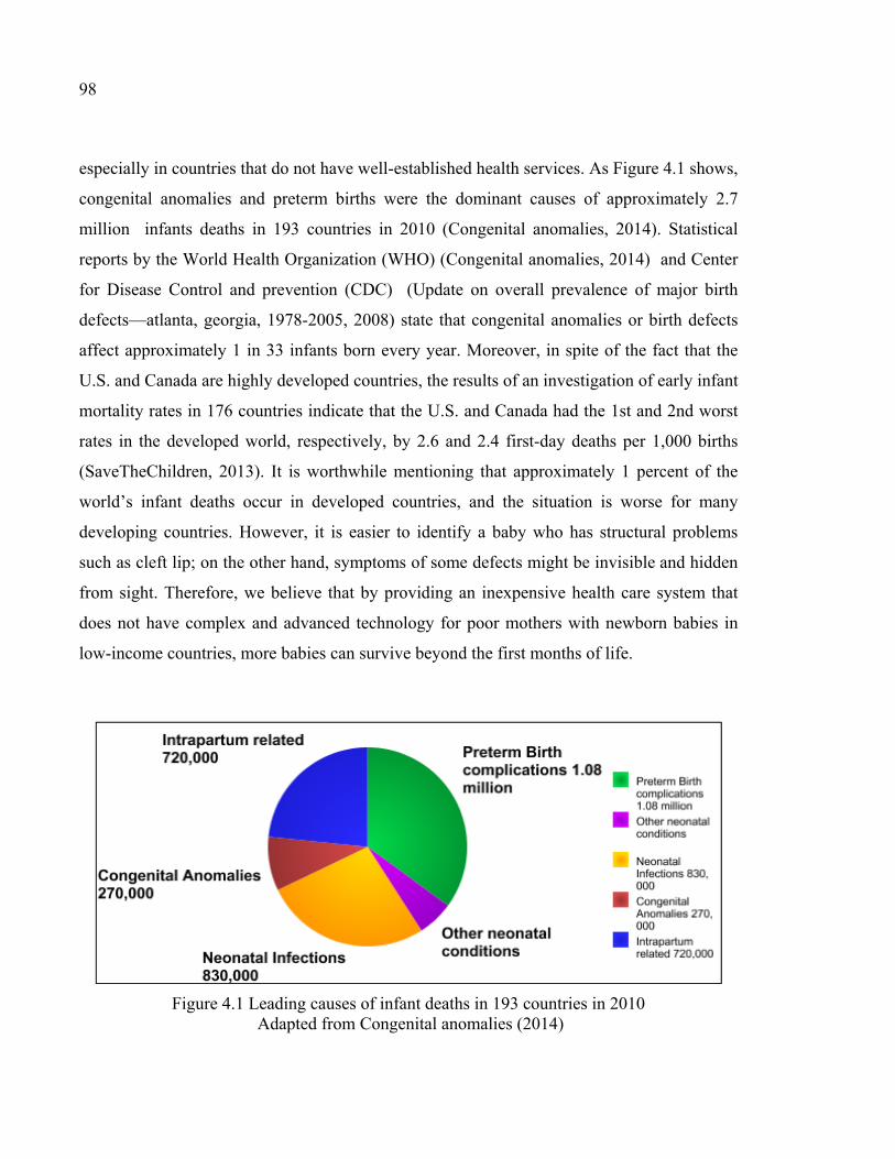
98
especially in countries that do not have well-established health services. As Figure 4.1 shows,
congenital anomalies and preterm births were the dominant causes of approximately 2.7
million infants deaths in 193 countries in 2010 (Congenital anomalies, 2014). Statistical
reports by the World Health Organization (WHO) (Congenital anomalies, 2014) and Center
for Disease Control and prevention (CDC) (Update on overall prevalence of major birth
defects—atlanta, georgia, 1978-2005, 2008) state that congenital anomalies or birth defects
affect approximately 1 in 33 infants born every year. Moreover, in spite of the fact that the
U.S. and Canada are highly developed countries, the results of an investigation of early infant
mortality rates in 176 countries indicate that the U.S. and Canada had the 1st and 2nd worst
rates in the developed world, respectively, by 2.6 and 2.4 first-day deaths per 1,000 births
(SaveTheChildren, 2013). It is worthwhile mentioning that approximately 1 percent of the
world’s infant deaths occur in developed countries, and the situation is worse for many
developing countries. However, it is easier to identify a baby who has structural problems
such as cleft lip; on the other hand, symptoms of some defects might be invisible and hidden
from sight. Therefore, we believe that by providing an inexpensive health care system that
does not have complex and advanced technology for poor mothers with newborn babies in
low-income countries, more babies can survive beyond the first months of life.
Figure 4.1 Leading causes of infant deaths in 193 countries in 2010 Adapted from Congenital anomalies (2014)
99
There are a substantial number of maternal and environmental issues that can raise the risks
of several complications and associated anomalies, such as the gestational age, birth weight,
consanguinity, maternal age, multiple gestations, and maternal infection during pregnancy,
socioeconomic factors and maternal nutritional status. For example, the gestational age is a
noteworthy predictor of infant health conditions within the normal range of 37-41 weeks for
babies who are fully developed (full term). Premature birth, even only a few weeks early,
increases the chance of birth defects or infant death in such a way that in the U.S., the 2010
mortality rate for very early preterm (under 32 weeks) births was 74 times worse than that of
full-term infants (T.J. et F. MacDorman, 2013).
These official statistics can provide more information about the chance that an infant is born
with a specific congenital disease, which is completely independent of the information in the
infant cries. Moreover, there are other independent sources of information that are related to
the physiological condition of the newborn infants that can be useful in a similar way in
multimodal biometric systems, which use multiple independent sources of information and
indeed provide a reliable system. However, in this article, we are curious about examining
only the ability of information that is embedded in infant cries to differentiate between
several pathologies in spite of the other sources.
This approach encouraged us to be ambitious and develop a newborn cry-based diagnostic
system for the care of birth defects after birth by identifying some possible physiological
disorders and birth defects. This early intervention can definitely save the lives of many
infants and protect them from some physical, intellectual, visual or auditory impairment
before severe disabilities might be caused.
100
4.2.2 Related studies
The leading role in the classification of the infant cry is how to scientifically discriminate
between different neonatal health statuses, only on the basis of their cry signals besides the
health examination of infants and other predictors of child health. In recent years, several
machine learning and classification algorithms, such as artificial neural networks (Cano et
al., 2006; Hariharan, Yaacob et Awang, 2011; Orozco et Garcia, 2003), radial basis function
(RBF) networks (Cano Ortiz, Escobedo Beceiro et Ekkel, 2004b), support vector machines
(SVMs) (Amaro-Camargo et Reyes-García, 2007), Naïve Bayes (Amaro-Camargo et Reyes-
García, 2007), Genetic Selection of a Fuzzy Model (GSFM) (Rosales-Pérez et al., 2012) have
demonstrated the ability to recognize cry patterns and make intelligent decisions based on the
available training databases. It is worthwhile mentioning that it is sometimes not easy to
collect a large number of samples to represent a general cry pattern. The failure to achieve
the lowest possible error rate is the main drawback of having no acceptable cry database. For
this reason, learning from a small, incomplete set of samples is of practical interest.
Finite mixture models is a flexible and powerful probabilistic tool for modeling univariate
and multivariate data to perform modeling and classification tasks (McLachlan et Peel,
2004). In this article, we employ the Gaussian mixture model (GMM), which is a powerful
model for representing almost any distribution. The Gaussian mixture model is
computationally inexpensive and is based on a well-understood statistical model that can be
viewed as a hybrid between a parametric and nonparametric density model. Moreover, there
are many advantages that are claimed when using GMM as the likelihood function
(Reynolds, Quatieri et Dunn, 2000). The expectation-maximization (EM) algorithm is a
common method for maximum likelihood learning of finite GMMs; this approach has some
advantages over other learning methods, such as a gradient-based approach (Xu et Jordan,
1996). In our previous studies (Farsaie Alaie et Tadj, 2012; 2013), we have introduced a
working prototype to train a GMM in an incremental and recursive manner; this method is
called the adapted boosted mixture learning Method (BML). The proposed method trains
finite mixture models by a pool of Gaussian components using an extracted Mel-frequency

101
Cepstral Coefficients (MFCCs) feature stream, which includes both static and dynamic
features. Partial and global updating methods are used in model parameter estimation
processes to speed up the learning process and converge to a more robust and reliable
estimation of a new mixture component. The selected strategy to stop the adding process is a
criterion-based approach called Bayesian Information Criterion (BIC). We have shown that
the proposed method has better performance than the traditional EM-based re-estimation
algorithm as a reference system for the classification of the infant cry. In a binary
classification task, the system discriminated a test infant’s cry signal into one of two groups,
namely, healthy and sick groups, based on MFCCs.
In this paper, we describe the development and evaluation of a Gaussian Mixture Model-
Universal Background Model (GMM-UBM) system that is applied to an infant cry expiration
and inspiration corpora for the enrolled health conditions. This newborn cry-based diagnostic
system can be referred to as the GMM-UBM health-condition detection system. The
remainder of this paper is organized as follows: In section 2, we present our cry database
(CDB). Next, in section 3, the feature extraction procedure is explained. Section 4 presents
our classification approach, and section 5 describes experiments and the results of each
health-condition detector using our cry database. Finally, conclusions and future directions
are presented in section 4.7.
4.3 Recording procedure and cry data base
The recordings were made in the neonatology departments of several hospitals in Canada and
Lebanon. We performed the recording process by converting the analog cry signal to an
uncompressed digital audio format that is suitable for storing an original recording in a wav
file. Each infant’s cry was recorded by an Olympus hand-held digital 2-channel recorder at a
sampling frequency of 44.1 kHz and a sample resolution of 16 bits, placed 10-30 cm away
from the infant’s mouth. A neonatal intensive-care unit (NICU) is a special system of care for
newborn infants who are sick or premature or generally need more medical attention due to
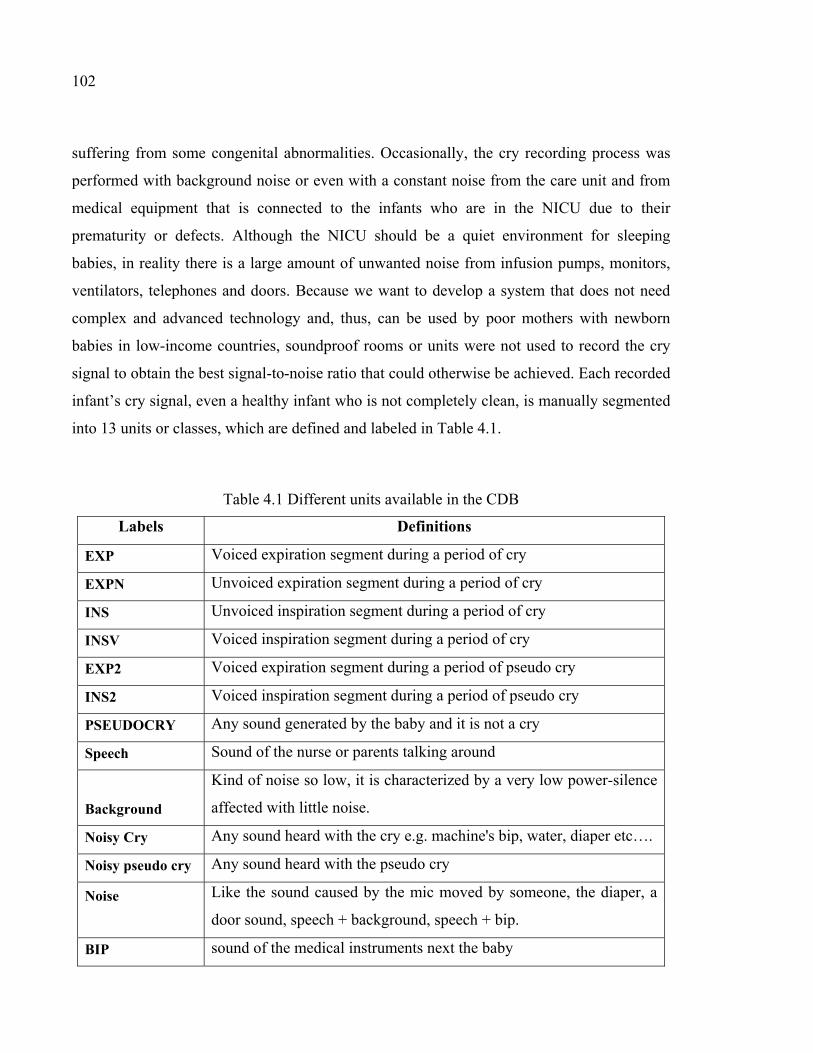
102
suffering from some congenital abnormalities. Occasionally, the cry recording process was
performed with background noise or even with a constant noise from the care unit and from
medical equipment that is connected to the infants who are in the NICU due to their
prematurity or defects. Although the NICU should be a quiet environment for sleeping
babies, in reality there is a large amount of unwanted noise from infusion pumps, monitors,
ventilators, telephones and doors. Because we want to develop a system that does not need
complex and advanced technology and, thus, can be used by poor mothers with newborn
babies in low-income countries, soundproof rooms or units were not used to record the cry
signal to obtain the best signal-to-noise ratio that could otherwise be achieved. Each recorded
infant’s cry signal, even a healthy infant who is not completely clean, is manually segmented
into 13 units or classes, which are defined and labeled in Table 4.1.
Table 4.1 Different units available in the CDB
Labels Definitions
EXP Voiced expiration segment during a period of cry
EXPN Unvoiced expiration segment during a period of cry
INS Unvoiced inspiration segment during a period of cry
INSV Voiced inspiration segment during a period of cry
EXP2 Voiced expiration segment during a period of pseudo cry
INS2 Voiced inspiration segment during a period of pseudo cry
PSEUDOCRY Any sound generated by the baby and it is not a cry
Speech Sound of the nurse or parents talking around
Background
Kind of noise so low, it is characterized by a very low power-silence
affected with little noise.
Noisy Cry Any sound heard with the cry e.g. machine's bip, water, diaper etc….
Noisy pseudo cry Any sound heard with the pseudo cry
Noise
Like the sound caused by the mic moved by someone, the diaper, a
door sound, speech + background, speech + bip.
BIP sound of the medical instruments next the baby

103
The case subjects for this study were infants selected from 1 to 53 days old, comprising
healthy and sick full-term babies. For each infant, there are three recording files, with the
average duration of 90 seconds for each continuous file. Useful information such as the date
of birth were recorded along with the following pertinent information: weight, gender,
maturity, race, ethnicity, gestational age, known and detected diseases, APGAR result, date
and time of each cry recording and the reason for the crying (such as pain, hunger, diaper
change, birth cry, medical exam).
We divided the available health conditions in our CDB into different categories listed in
Table 4.2. The reason for the cry is not considered in the selected samples, in contrast to
previous studies that used only the pain cry (Partanen et al., 1967).
Table 4.2 List of health-conditions
Categories Describtion
Healthy infants Fullterm infants without any major disorder or sickness
Heart problems Fullterm infants suffering from Tetralogy of Fallot, thrombus,
complex cardio or congenital heart diseases.
Neurological Fullterm infants suffering from Sepsis or Meningitis.
Respiratory distress Fullterm infants suffering from Respiratory distress or
Asphyxia diseases.
Blood abnormalities Fullterm infants suffering from Hyperbilirubinemia or
Hypoglycemia diseases.
Other Fullterm infants suffering from other abnormalities or physical
problems which are not in priority order for our system.
4.4 Feature extraction
Usually, in human speech signals, there are low-level and high-level cues that can be used to
recognize different speakers; these cues are related to the acoustic and semantic or linguistic

104
aspects of speech. The human auditory system uses different levels of information, in
contrast to automatic systems, which depend still on low-level acoustic information.
The major challenges of having a higher level of information derived from a cry signal are to
find and extract some features in such a way that they convey distinctive information from
the cry signal; this approach has been under study in recent years (Kheddache, 2014). In this
article, MFCCs are selected to be extracted as features that represent the cry signals because
they have good performance among various types of speech applications (Deller, Proakis et
Hansen, 1993; Quatieri, 2002). Note that the same basic model of speech production (Deller,
Proakis et Hansen, 1993) in adults is used to find these measurements. Thus far, it has been
shown that they are also effective in classifying healthy and sick infants based on our
primary results (Farsaie Alaie et Tadj, 2012). Moreover, we incorporate context information
by adding dynamic features in the second step, but they are not necessarily the most
informative features for the intended pathology classification task.
4.4.1 Preprocessing stages
To increase the accuracy and reliability of the MFCC feature extraction process, cry signals
are pre-processed in 3 simple steps:
1. Convert stereo channel to mono channel
In the data collection step, because we have used a 2-channel recorder, we must average the
channels first and then convert the signal into a single-channel signal using a mean value
function.
2. Pre-emphasization
Similar to in a speech recognition system, we used a first-order high-pass FIR filter to pre-
emphasize the signal due to the high dynamic range of the digitized cry waveform, such as in
105
a speech waveform. The main reason for using this filter is to compensate the spectral effect
of the glottal source by introducing a zero near = 1 (Deller, Proakis et Hansen, 1993).
Therefore, the filter ( ) 1P z 1 0.97z−= − (Rabiner et Schafer, 1978; Young et al., 2006a) should be
applied prior to deriving the features or characteristics that correspond to the vocal tract only.
3. EXP/INSV detection
Although a cry is defined as the expiratory phase of respiration with sound or phonation by
the larynx, which contains the vocal cords or folds and the glottis (LaGasse, Neal et Lester,
2005), here the input that is given to our cry-based diagnostic system (cry pathology
classifier) represents a processed version of one or more voiced expiration (EXP) or
inspiration (INSV) segments of cry utterances called feature vectors. Therefore, after
segmentation and labeling, only the EXP and INSV segments of the cry signals are selected
for the feature extraction procedures. The system has been built manually by trained experts
so far, but we are working on automatic segmentation of recorded cry signals that can act
instead of voice activation detection (VAD) in speech recognition systems.
4.4.2 Static and dynamic MFCCs
Briefly, the cry signals are pre-processed to be prepared for short-term processing, and then,
the feature extraction procedure is applied, including MFCCs, delta and delta-delta
coefficients. Generally, all of the conventional analysis techniques used in the signal
processing application work with short-term frames of signals with non-stationary dynamics,
such as human speech. Therefore, even in our case in point, it is our duty to select a
reasonable portion of the cry signal in such a way that it does not change statistically. Frames
are commonly 10-30 msec in duration, to be statistically stationary with a good tradeoff
between the frequency and time resolutions in applications that use speech signals. In this
article, feature extraction was performed by using two different frame durations, 10 and 30,
with the same overlap percentage (30%) between two consecutive windows, to find a good
tradeoff between the frequency and time resolution of the cry signals and to assess what
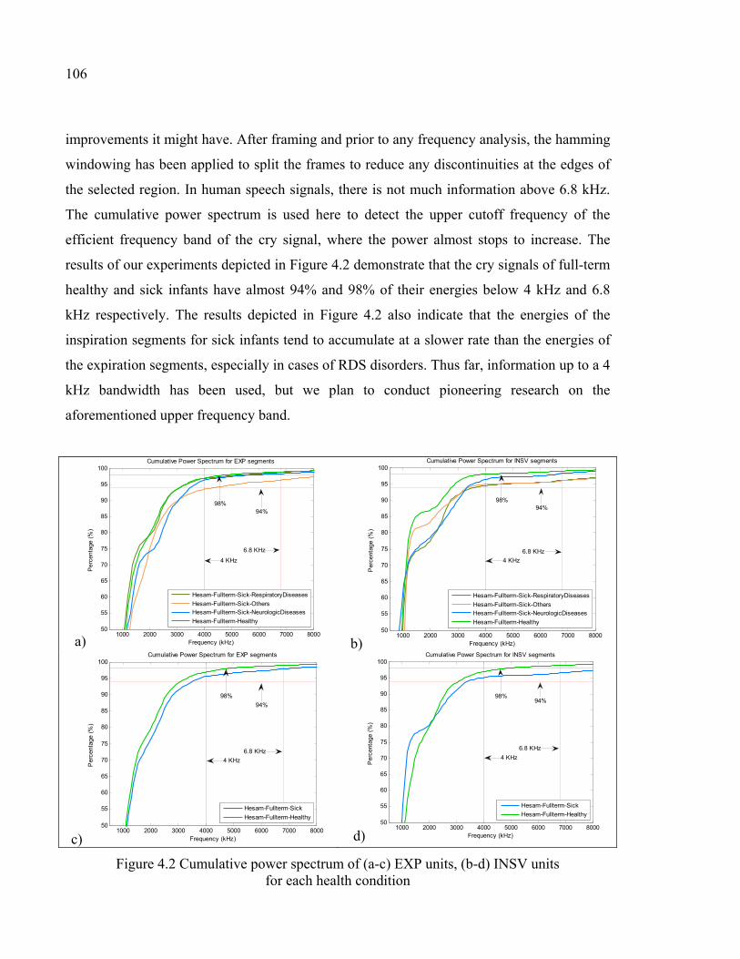
106
improvements it might have. After framing and prior to any frequency analysis, the hamming
windowing has been applied to split the frames to reduce any discontinuities at the edges of
the selected region. In human speech signals, there is not much information above 6.8 kHz.
The cumulative power spectrum is used here to detect the upper cutoff frequency of the
efficient frequency band of the cry signal, where the power almost stops to increase. The
results of our experiments depicted in Figure 4.2 demonstrate that the cry signals of full-term
healthy and sick infants have almost 94% and 98% of their energies below 4 kHz and 6.8
kHz respectively. The results depicted in Figure 4.2 also indicate that the energies of the
inspiration segments for sick infants tend to accumulate at a slower rate than the energies of
the expiration segments, especially in cases of RDS disorders. Thus far, information up to a 4
kHz bandwidth has been used, but we plan to conduct pioneering research on the
aforementioned upper frequency band.
a) b)
c) d)
Figure 4.2 Cumulative power spectrum of (a-c) EXP units, (b-d) INSV units for each health condition
1000 2000 3000 4000 5000 6000 7000 800050
55
60
65
70
75
80
85
90
95
100Cumulative Power Spectrum for EXP segments
Per
cent
age
(%)
Frequency (kHz)
Hesam-Fullterm-Sick-RespiratoryDiseases
Hesam-Fullterm-Sick-OthersHesam-Fullterm-Sick-NeurologicDiseases
Hesam-Fullterm-Healthy
4 KHz
6.8 KHz
98%94%
1000 2000 3000 4000 5000 6000 7000 800050
55
60
65
70
75
80
85
90
95
100Cumulative Power Spectrum for INSV segments
Per
cent
age
(%)
Frequency (kHz)
Hesam-Fullterm-Sick-RespiratoryDiseases
Hesam-Fullterm-Sick-OthersHesam-Fullterm-Sick-NeurologicDiseases
Hesam-Fullterm-Healthy
4 KHz
6.8 KHz
98%94%
1000 2000 3000 4000 5000 6000 7000 800050
55
60
65
70
75
80
85
90
95
100Cumulative Power Spectrum for EXP segments
Per
cent
age
(%)
Frequency (kHz)
Hesam-Fullterm-Sick
Hesam-Fullterm-Healthy
4 KHz
6.8 KHz
98%
94%
1000 2000 3000 4000 5000 6000 7000 800050
55
60
65
70
75
80
85
90
95
100Cumulative Power Spectrum for INSV segments
Per
cent
age
(%)
Frequency (kHz)
Hesam-Fullterm-Sick
Hesam-Fullterm-Healthy
4 KHz
6.8 KHz
98%94%

107
In brief, the feature extraction phase for both the INSV and EXP segments can be performed
in two stages:
1. Reduce the dimensionality by Cepstral analysis and extract the first 12 MFCCs computed
from 24 filter banks plus the energy feature.
MFCCs are introduced by Mermelstein in (Davis et Mermelstein, 1980) as the DCT of the
log-energy output of the triangular band pass filters. To extract the MFCCs, first the fast
Fourier Transform (FFT) is performed to obtain the magnitude frequency of each windowed
frame, and then, the MFCCs are calculated by converting the log Mel spectrum back to the
time domain using the discrete cosine transform (DCT):
= ∑ cos[ ( − ) ] , = 1,2, … , (4.1)
where K is number of subbands (filter banks) (which is 24 for our selected bandwidth
(Reynolds, 1995a)), is the desired length of the cepstrum, and represents the log-energy
output of the th triangular band pass filter. Figure 4.3 indicates all of the 3 pre-processing
steps followed by the aforementioned MFCC extraction procedure in stages.
Figure 4.3 Pre-processing and MFCC feature extraction steps
2. Add dynamic features by taking the first and second derivatives of the obtained 13-static
features, called the delta and delta-delta (acceleration) coefficients.
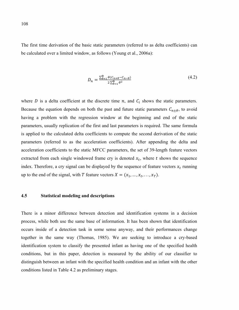
108
The first time derivation of the basic static parameters (referred to as delta coefficients) can
be calculated over a limited window, as follows (Young et al., 2006a):
= ∑ ( )∑ (4.2)
where is a delta coefficient at the discrete time , and shows the static parameters.
Because the equation depends on both the past and future static parameters ± , to avoid
having a problem with the regression window at the beginning and end of the static
parameters, usually replication of the first and last parameters is required. The same formula
is applied to the calculated delta coefficients to compute the second derivation of the static
parameters (referred to as the acceleration coefficients). After appending the delta and
acceleration coefficients to the static MFCC parameters, the set of 39-length feature vectors
extracted from each single windowed frame cry is denoted , where shows the sequence
index. Therefore, a cry signal can be displayed by the sequence of feature vectors running
up to the end of the signal, with feature vectors = ( ,… , , . . . , ).
4.5 Statistical modeling and descriptions
There is a minor difference between detection and identification systems in a decision
process, while both use the same base of information. It has been shown that identification
occurs inside of a detection task in some sense anyway, and their performances change
together in the same way (Thomas, 1985). We are seeking to introduce a cry-based
identification system to classify the presented infant as having one of the specified health
conditions, but in this paper, detection is measured by the ability of our classifier to
distinguish between an infant with the specified health condition and an infant with the other
conditions listed in Table 4.2 as preliminary stages.
109
4.5.1 Likelihood ratio detector
In an ideal case and with well-defined models for all newborn infant pathologies and health
conditions, the defined classification problem is similar to the canonical language recognition
problem (Brummer, 2010) with the closed-set of specified languages. Similar to speaker
identification systems that are intended for a 1:N match, the voice is compared against N
speaker models ( , , … , ), where represents the parameters of the speaker model.
This system can be presented by a maximum likelihood classifier whose objective is to select
the speaker model that has the maximum a posteriori probability (MAP) for the observation
vector sequence = ( ,… , , . . . , ). The decision can be presented by the minimum-
error Bayes’ rule, as follows:
MatchedSpeaker Index = argmax ( | ) = argmax ( | ) ( )( ) (4.3)
You can also make an assumption on the prior probability of each speaker to simplify the
approach. This assumption is called the assumption of equal prior probabilities of speakers,
which results in making the decision formula as follows:
MatchedSpeakerIndex = argmax p(X|λ ) = argmax ∑ log p(x |λ ) (4.4)
In verification systems, the task is a 1:1 match, which is in marked contrast to the
identification system. For example, in speaker verification systems, the objective is to
determine if the observed input is from the hypothesized speaker (hypothesis ) or not
(hypothesis ). The likelihood ratio detector has been accepted as a general approach in the
speaker verification system (Reynolds, Quatieri et Dunn, 2000). Assume that and
hypotheses are represented by models and , respectively; it calculates the ratio of
the posterior probabilities of the two hypotheses:
110
( | )( | ) (4.5)
Bayes’ rule provides a shortcut for calculating the likelihood ratio in the log domain by
ignoring constants that result in the log-likelihood ratios of and , as follows:
( ) = log ( ) − log ⋛ θ (4.6)
where is a threshold that adjusts the trade-off between two types of error, false acceptance
and false rejection. Although the claimed speaker has a well-defined model in such a system,
the corresponding alternative models are ill-defined. This issue poses a challenge to create
in such a way that presents the entire space of possible alternatives to the hypothesized
speaker. In general, two main approaches have been described in (Reynolds, Quatieri et
Dunn, 2000) to model . Because we used both techniques in our cry-based diagnostic
pathology system, we describe both of them briefly below.
1. Background Speaker Models
In this approach, the set of speaker models excluding the hypothesized speaker have been
selected and combined to model the alternative hypothesis. There has been a large amount of
research into background speakers (Higgins, Bahler et Porter, 1991; Matsui et Furui, 1994;
Reynolds, 1995b; Rosenberg et al., 1992). Given equally likely background speakers,
which are represented by ( , , … , ), the log-likelihoods of the hypothesized speaker and
alternative hypothesis (background speakers) are computed as (Reynolds, 1995b)
log ( ) = ∑ log p(x λ ) (4.7)
111
The 1/ factor is used to normalize the duration effect in the log-likelihood. Note that by
ignoring the 1/ factor, the likelihood of the background speakers can be observed as the
joint probability density of the observation arising from one of the background speakers:
log ( ) = log( ∑ p(X|λ )) (4.8)
where ( | ) is computed as in Equation 4.7. The main drawback of this approach is
preparing a background speaker set for each hypothesized speaker, which can be a problem
for applications that have a large number of hypotheses.
2. Speaker-Independent Model
This technique (Matsui et Furui, 1995; Reynolds, 1997) attempts to pool training samples
from a large number of speakers, to represent the population of speakers by a single speaker-
independent model; this model is currently known as a universal background model (UBM).
A Universal Background Model (UBM) is a world model that is used mostly in biometric
verification systems to represent general feature characteristics (Reynolds, 2009).
Specifically, the universal-background model-based GMM or GMM-UBM has a large
amount of success in statistical modeling techniques for speaker recognition and language
recognition systems (Reynolds, Quatieri et Dunn, 2000), and in contrast to previous
approaches, a trained UBM can be used for all hypothesized speakers in the task.
4.5.2 Gaussian mixture models
The GMM modeling technique is simple but effective due to its remarkable ability to form
smooth approximations from any arbitrarily shaped data distribution. It has been a success as
a statistical model in different applications and systems, most notably in speaker recognition
and speaker identification systems (Reynolds et Rose, 1995) due to its ability to model the
112
underlying data classes or distributions of acoustic observations from a speaker. The
likelihood function of a GMM used for a D-dimensional feature vector, x, is a weighted sum
of unimodal Gaussian components, ( ), each parameterized by a mean × 1 mean
vector ( ) and a × covariance matrix ( ), as given by the equation
( | ) = ∑ ( ) = ∑ ( | ) = ∑ ( | , ) (4.9)
where represents the GMM parameters and consists of components with the restriction
that the mixture weights must satisfy the following two constraints: ≥ 0 for = 1,… ,
and ∑ = 1. The component can be written in the following notation:
( ) = ( | ) = ( | , ) = ( ) | | × − ( − ) ( − )
(4.10)
where = ( , ) are the parameters for the Gaussian density, and represents the
transpose of matrix A. Collectively, a GMM can be denoted by its parameters as =( , , = 1, . . , ).
4.5.3 System description
The proposed diagnostic system is built around the likelihood ratio test for detection by using
GMMs for likelihood functions and GMM-UBM models to derive speaker models from the
related world models. In the related literature, the common method to derive speaker models
is called Bayesian learning or the MAP estimation method (Duda et Hart, 1973; Gauvain et
Chin-Hui, 1994; Reynolds, Quatieri et Dunn, 2000). In our NCDS, the UBM is a health-
independent GMM that is trained with cry samples from the available training CDB that
contains full-term healthy and sick infants with specific diseases, to represent the general cry
feature characteristics. Then, we employed the adapted BML method to adapt the UBM to a
113
target or specific class. We will show that this approach improves the performance of our
classifier in comparison to our reference system, which uses Bayesian adaptation.
The first part of our system acts as a verification system for healthy infants, while
distinguishing between healthy infants and sick infants. The goal here is to determine
whether the infant is healthy or not; in the case of unhealthy, the second part should act as an
identification system because the cry signals of the sick infants are assumed to be from the
predefined set of known sicknesses. The winner sickness best matches the test infant’s cry
signal model in a known group of diseases. This sickness identification system involves only
the aforementioned enrolled sicknesses and not all of the newborn illnesses. In the closed-set
case, ( , , … , ) represents L different infant sicknesses, which have well-defined
statistical models. In the second scenario, which is called the open-set, the same ( , , … , ) are specified sicknesses, and denotes any of the unseen out-of-set
sicknesses. Therefore, we created a class called “others” or “none-of-the-above” in the target
set of diseases. The state-of-the-art infant’s cry-based health care system has a hierarchical
scheme that is composed of two subsystems that are both based on an acoustic approach.
Individual scores for expiration-based and inspiration-based experts are fused together to
exploit the complementary information that can be represented by our health care system
defined over the features extracted from two different types of corpora.
The crux of the design is how we fuse subsystems into a single effective system. Our cry-
based multi-class recognition system has a hierarchical scheme that is a treelike combination
of individual classifiers in serial and parallel modes. We used the ability of the serial mode to
narrow down the health condition of the infants to one of two possibilities, such as the
biometric identification system introduced in (Hong et Jain, 1998). This approach means that
in the first step, the two-class pattern recognizer should make the decision as to which
proposition should be eliminated, healthy or sick infants. For healthy infants, the decision
process should be stopped at this stage before using all of the remaining classifiers that can
reduce the overall recognition time. Then, in the case of sick infants, two individual pattern

114
recognizers in a parallel mode of operation should arrive at a final decision on the
pathological condition of the test infant. In case the accuracy of the final decision on the most
likely disease was called into doubt, there is another class called others that corresponds to
infants that do not have the considered diseases or those for which we need more recorded
cry signals for more examination.
The proposed detection system works in two phases, which are called training and runtime
test. In the first phase, labeled cry corpora are analyzed and used to train the corresponding
model. Each model should represent some health-dependent characteristics of the training
data. In the test phase, the presented cry sample goes through the same process as in the
training phase (the preprocessing and feature extraction steps), and then, for both the
expiration and inspiration corpora of the sample, the log-likelihood ratio to the hypothesized
model is calculated. In the decision stage of the system, we use different methods (SVM,
PNN, and MLP) to fuse these scores to improve the performance of the classifier.
4.5.4 Applying the GMM-UBM
In this article, we defined and trained two GMM-UBMs for each corpora (EXP and INSV),
based on the health conditions; the first one is a single health-independent background model
trained to represent the distribution of the extracted cry features, regardless of what condition
the infant might have (healthy or sick), and the second one is a pathology-independent
background model that attempts to model cry features from all of the sicknesses that are
available in our CDB. Because we focus our attention on full-term healthy and sick newborn
infants that have specific diseases, we train the UBM to be used for the classification of
healthy and sick infants using only corresponding data that are reflective of the expected
alternative cry to be encountered during recognition. For example, in this case, it is known a
priori that the cry signal belongs to a full-term infant, and thus, the full-term test infant will
only be classified against full-term infant cries. This approach applies to both the gestational
age of the infants and the types of diseases that are considered in our case.
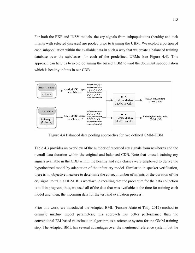
115
For both the EXP and INSV models, the cry signals from subpopulations (healthy and sick
infants with selected diseases) are pooled prior to training the UBM. We exploit a portion of
each subpopulation within the available data in such a way that we create a balanced training
database over the subclasses for each of the predefined UBMs (see Figure 4.4). This
approach can help us to avoid obtaining the biased UBM toward the dominant subpopulation
which is healthy infants in our CDB.
Figure 4.4 Balanced data pooling approaches for two defined GMM-UBM
Table 4.3 provides an overview of the number of recorded cry signals from newborns and the
overall data duration within the original and balanced CDB. Note that unused training cry
signals available in the CDB within the healthy and sick classes were employed to derive the
hypothesized model by adaptation of the infant cry model. Similar to in speaker verification,
there is no objective measure to determine the correct number of infants or the duration of the
cry signal to train a UBM. It is worthwhile recalling that the procedure for the data collection
is still in progress; thus, we used all of the data that was available at the time for training each
model and, then, the incoming data for the test and evaluation process.
Prior this work, we introduced the Adapted BML (Farsaie Alaie et Tadj, 2012) method to
estimate mixture model parameters; this approach has better performance than the
conventional EM-based re-estimation algorithm as a reference system for the GMM training
step. The Adapted BML has several advantages over the mentioned reference system, but the
116
distinct advantage is that it estimates the optimum number of components by iteratively
adding new components in the direction that largely increases the predefined objective
function. There is no guarantee that increasing the number of components in a GMM trained
by HTK provides better system accuracy (Dobrovic et al., 2012), although the EM algorithm
(Dempster, Laird et Rubin, 1977) iteratively re-estimates the GMM parameters to
monotonically increase the likelihood of the model for the vector of observations, in contrast
to the adapted-BML, in which each new added component brings improvement in the
predefined objective function. Despite this option, in the preliminary stages of our cry-based
diagnostic system, the building or training phase of the defined GMM-UBMs has been
performed based on the HTK (Hidden Markov Model Toolkit) software tool, which is an
established tool of speech recognition systems based on hidden Markov models (Young et
al., 2006a). In the training procedure, we substitute diagonal covariance matrices for the full
covariance matrices due to its computational efficiency because a diagonal covariance GMM
with order > 1 can model distributions of feature vectors with correlated elements. Then,
in the next step, we used the adapted version of the parameter updating procedure described
in (Farsaie Alaie et Tadj, 2012) to adapt UBM to create specific health condition models.
4.5.5 BML adaptation of sub-models or health-dependent-infant cry model
As mentioned earlier, there is a common technique called Bayesian adaptation (Duda et Hart,
1973; Gauvain et Chin-Hui, 1994) for deriving the hypothesized speaker model from GMM-
UBM. Here, we introduce a new way of updating the GMM-UBM parameters based on the
infant cry signals from related subclasses. In fact, a part of this adaptation technique was
introduced earlier in (Farsaie Alaie et Tadj, 2012; Jun, Yu et Hui, 2011) as partial and global
updating in Boosted mixture learning (BML) of GMM and HMM-based acoustic models.
Specifically, we use the concept of boosting to refine the UBM parameters using the training
cry signals of a specific health condition.
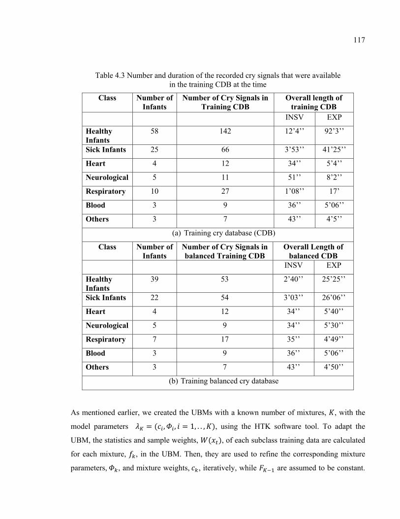
117
Table 4.3 Number and duration of the recorded cry signals that were available in the training CDB at the time
Class Number of Infants
Number of Cry Signals in Training CDB
Overall length of training CDB
INSV EXP
Healthy Infants
58 142 12’4’’ 92’3’’
Sick Infants 25 66 3’53’’ 41’25’’
Heart 4 12 34’’ 5’4’’
Neurological 5 11 51’’ 8’2’’
Respiratory 10 27 1’08’’ 17’
Blood 3 9 36’’ 5’06’’
Others 3 7 43’’ 4’5’’
(a) Training cry database (CDB)
Class Number of Infants
Number of Cry Signals in balanced Training CDB
Overall Length of balanced CDB
INSV EXP
Healthy Infants
39 53 2’40’’ 25’25’’
Sick Infants 22 54 3’03’’ 26’06’’
Heart 4 12 34’’ 5’40’’
Neurological 5 9 34’’ 5’30’’
Respiratory 7 17 35’’ 4’49’’
Blood 3 9 36’’ 5’06’’
Others 3 7 43’’ 4’50’’
(b) Training balanced cry database
As mentioned earlier, we created the UBMs with a known number of mixtures, , with the
model parameters = ( , , = 1, . . , ), using the HTK software tool. To adapt the
UBM, the statistics and sample weights, ( ), of each subclass training data are calculated
for each mixture, , in the UBM. Then, they are used to refine the corresponding mixture
parameters, , and mixture weights, , iteratively, while are assumed to be constant.

118
By applying the EM algorithm to optimize the log-likelihood of the model for the vector of
observations only with respect to the mixture component , the iterative formula can be
derived to adapt the model parameters. The adapted parameters, = ( ̂ , , = 1, . . , ), can be estimated in the ( + 1) equation as follows:
( )
( )( )( )( ) ( ) ( )
( )( )( )
1 1
1
n nk t k k t k
nt nn n
k t kk k t k k k t k
X Xw X
F Xc X c
f
F
f
f X λλ− −
Φ Φ= =
Φ + −
(4.11)
( )( ) ( )( )
1
nn t
t k T ntt
w X
w Xγ
=
Φ =
(4.12)
( )1
1
1ˆ ˆ
Tn n n
k k tt
c c w XT
+
=
= (4.13)
( )( )1
1
ˆ .T
nnk t k t
t
Xμ γ+
=
= Φ (4.14)
( )( ) ( )( )1 1 1
1
ˆ ˆ ˆ. T Trnn n n
k t k t k t kt
X Xγ μ μ+ + +
=
Σ = Φ − − (4.15)
in which the UBM parameters are used as an initial point. The adaptation procedure is
performed in such a way that mixtures with a high count of subclass training data concentrate
more on these examples, and vice versa. In other words, due to the existence of in the
numerator and in the denominator of the weight samples equation, the observations that
have lower probabilities by the model are given larger weights than those that have
higher probabilities. It is worthwhile mentioning that the first part of the denominator can
reduce the probability of the case in which is dominated by a few samples. Moreover,
sample weights in the updating mixture weights formula act as a tuning parameter, which
helps to rectify the mixture weights iteratively by determining the ability of each mixture
component to model the subclass training samples.
In comparison to the clear coupling method presented in Bayesian adaptation (Gauvain et
Chin-Hui, 1994; Reynolds, Quatieri et Dunn, 2000), the BML adaptation can be observed as
an indirect or hidden coupling between both the mixture weights and the parameters of the
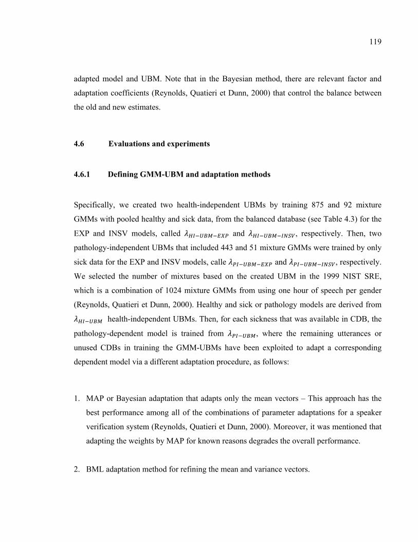
119
adapted model and UBM. Note that in the Bayesian method, there are relevant factor and
adaptation coefficients (Reynolds, Quatieri et Dunn, 2000) that control the balance between
the old and new estimates.
4.6 Evaluations and experiments
4.6.1 Defining GMM-UBM and adaptation methods
Specifically, we created two health-independent UBMs by training 875 and 92 mixture
GMMs with pooled healthy and sick data, from the balanced database (see Table 4.3) for the
EXP and INSV models, called and , respectively. Then, two
pathology-independent UBMs that included 443 and 51 mixture GMMs were trained by only
sick data for the EXP and INSV models, calle and , respectively.
We selected the number of mixtures based on the created UBM in the 1999 NIST SRE,
which is a combination of 1024 mixture GMMs from using one hour of speech per gender
(Reynolds, Quatieri et Dunn, 2000). Healthy and sick or pathology models are derived from
health-independent UBMs. Then, for each sickness that was available in CDB, the
pathology-dependent model is trained from , where the remaining utterances or
unused CDBs in training the GMM-UBMs have been exploited to adapt a corresponding
dependent model via a different adaptation procedure, as follows:
1. MAP or Bayesian adaptation that adapts only the mean vectors – This approach has the
best performance among all of the combinations of parameter adaptations for a speaker
verification system (Reynolds, Quatieri et Dunn, 2000). Moreover, it was mentioned that
adapting the weights by MAP for known reasons degrades the overall performance.
2. BML adaptation method for refining the mean and variance vectors.

120
3. Coupling old and BML adaptation estimates over the mean and variance vectors – We
compute new statistics for the parameters based on the BML model estimates, and we use
a single adaptation coefficient for both the mean and variance parameters = with
the relevant factor = 16 to control the balance, which is the same as in Bayesian
adaptation.
4. BML adaptation method for refining only the mean vectors.
It is obvious that while adapting UBM to derive the GMM models for two
pathological conditions namely heart and blood disease, we utilized the same training data as
was used in HTK for training UBM, while for other diseases we used unseen data
that remained in our CDB.
4.6.2 Log-likelihood score computation
We applied the idea of the HNORM score normalization method described in (Reynolds,
1997) for the EXP and INSV cry units separately. In each health-condition detector, we used
only non-hypothesized or non-target cry samples (imposter) to estimate the normalization
parameters. Therefore, the non-target log-likelihood ratio score distributions have been
rescaled to have a mean of zero and a standard deviation of one. Due to different lengths of
extracted EXP/INSV segments from each recorded cry signal, more evidence might be
needed to make a reliable decision for each test file, especially for the INSV cry type, which
has a shorter duration than the EXP type. Therefore, each corpus was split into small cry
units of approximately 3 seconds duration to investigate the effect of the EXP/INSV duration
length in each recorded file. The results indicate that independent of the frame length, type of
cry units (EXP/INSV), adaptation method and task of the detector, recorded files that have
more 3 sec-length EXP/INSV cry units have more separable LLR scores (see Figure 4.5). In
other words, the more information that is available (EXP/INSV length inside each file), the
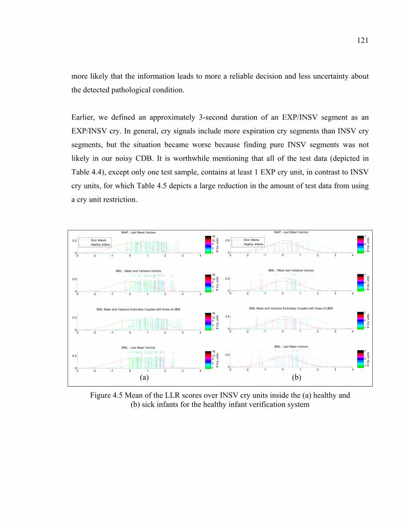
121
more likely that the information leads to more a reliable decision and less uncertainty about
the detected pathological condition.
Earlier, we defined an approximately 3-second duration of an EXP/INSV segment as an
EXP/INSV cry. In general, cry signals include more expiration cry segments than INSV cry
segments, but the situation became worse because finding pure INSV segments was not
likely in our noisy CDB. It is worthwhile mentioning that all of the test data (depicted in
Table 4.4), except only one test sample, contains at least 1 EXP cry unit, in contrast to INSV
cry units, for which Table 4.5 depicts a large reduction in the amount of test data from using
a cry unit restriction.
(a) (b)
Figure 4.5 Mean of the LLR scores over INSV cry units inside the (a) healthy and (b) sick infants for the healthy infant verification system
-3 -2 -1 0 1 2 3 40
0.5
MAP - Just Mean Vectors
# C
ry u
nits
1
5
912
16Sick Infants
Healthy Infants
-3 -2 -1 0 1 2 3 40
0.5
BML - Mean and Variance Vectors
# C
ry u
nits
1
5
912
16
-3 -2 -1 0 1 2 3 40
0.5
BML Mean and Variance Estimates Coupled with those of UBM
# C
ry u
nits
1
5
912
16
-3 -2 -1 0 1 2 3 40
0.5
BML - Just Mean Vectors
# C
ry u
nits
1
5
912
16
-3 -2 -1 0 1 2 3 40
0.5
MAP - Just Mean Vectors
# C
ry u
nits
1
4
7Sick Infants
Healthy Infants
-3 -2 -1 0 1 2 3 40
0.5
BML - Mean and Variance Vectors
# C
ry u
nits
1
4
7
-3 -2 -1 0 1 2 3 40
0.5
BML Mean and Variance Estimates Coupled with those of UBM
# C
ry u
nits
1
4
7
-3 -2 -1 0 1 2 3 40
0.5
BML - Just Mean Vectors
# C
ry u
nits
1
4
7

122
Table 4.4 Number of infants and recorded cry signals available in the testing CDB at the time
Class Number of Infants Number of Cry Signals in Testing CDB Healthy Infants
42 (4 male) 89 (11 male)
Sick Infants 40 101 Heart 2 (2 male) 3 (3 male) Neurological 11 (6 male) 30 (18 male) Respiratory 18 (12 male) 49 (35 male) Blood 4 (4 male) 9 (9 male) Others 4 (2 male) 10 (4 male)
Table 4.5 Number of cry samples that contain EXP/INSV-labeled segments and 3-sec cry units in our test CDB
Number of cry samples in the test cry database Class
Tot
al # Samples with
INSV-labeled segments # Samples with
at least 1 INSV unit
Healthy Infants
89 86 66
Sick Infants 101 93 62
Hea
rt
Neu
ro
Res
p
Blo
od
Oth
ers
Hea
rt
Neu
ro
Res
p
Blo
od
Oth
ers
a/b: a from b 1/3 29/30 45/49 9/9 9/10 1/3 22/30 24/49 7/9 8/10
(a) Inspiratory cry segments
Number of cry samples in the test cry database
Class
Tot
al # Samples with
EXP-labeled segments # Samples with
at least 1 EXP unit
Healthy
Infants
89 88 88
Sick Infants 101 101 101
Hea
rt
Neu
ro
Res
p
Blo
od
Oth
ers
Hea
rt
Neu
ro
Res
p
Blo
od
Oth
ers
a/b: a from b 3/3 30/30 49/49 9/9 10/10 3/3 30/30 49/49 9/9 10/10
(b) Expiratory cry segments

123
4.6.3 Health-condition detection system
In this section, we present the results of both healthy and sick (with specific diseases) infant
detection.
4.6.3.1 Healthy infant detector
We present only the results of our healthy infant detector for a test database using both test
EXP and INSV cry units with two different frame lengths (10 msec and 30 msec). Moreover,
to describe the entire space of possible alternatives for the healthy class, two explained
approaches, called background speaker modes ( = ( , , … , )) and UBM (λ ), have been used to compute the LLR scores. Because some of the test data do not have 3-sec
INSV cry units, to evaluate the detector based on the INSV models, we performed our
experiments on two sets of test data (see Table 4.5): 1) containing INSV-labeled segments
with any length and 2) containing at least one 3-sec INSV unit. On the other hand, almost all
of the data from the test database contains pure EXP-labeled segments except for one sample,
and thus, there are 88 healthy and 101 sick samples with EXP cry units for the evaluation
procedure. Here, we only present the results of data that contains 3-sec EXP/INSV cry units,
which are more satisfactory, as expected. The miss (false negative) and false alarm (false
positive) rates are, respectively, plotted on the x- and y-axis, which are scaled non-linearly
(normal deviate scale) as detection error tradeoff (DET) curves (Martin et al., 1997). The
DET plots that are depicted in Figure 4.6 and Figure 4.7 distinguish more clearly the
performance of the systems that have different adaptation methods, frame lengths, cry unit
types and representatives for the alternative health conditions.
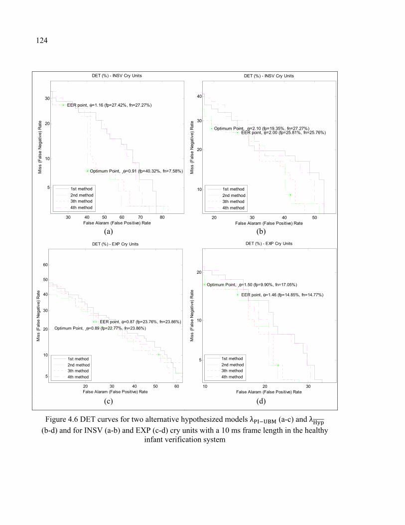
124
(a) (b)
(c) (d)
Figure 4.6 DET curves for two alternative hypothesized models λ (a-c) and λ
(b-d) and for INSV (a-b) and EXP (c-d) cry units with a 10 ms frame length in the healthy infant verification system
30 40 50 60 70 80
5
10
20
30
False Alaram (False Positive) Rate
Mis
s (F
alse
Neg
ativ
e) R
ate
DET (%) - INSV Cry Units
Optimum Point, ¸θ=0.91 (fp=40.32%, fn=7.58%)
EER point, θ=1.16 (fp=27.42%, fn=27.27%)
1st method
2nd method3th method
4th method
20 30 40 50
10
20
30
40
False Alaram (False Positive) Rate
Mis
s (F
alse
Neg
ativ
e) R
ate
DET (%) - INSV Cry Units
Optimum Point, ¸θ=2.10 (fp=19.35%, fn=27.27%) EER point, θ=2.00 (fp=25.81%, fn=25.76%)
1st method
2nd method3th method
4th method
20 30 40 50 60
5
10
20
30
40
50
60
False Alaram (False Positive) Rate
Mis
s (F
alse
Neg
ativ
e) R
ate
DET (%) - EXP Cry Units
Optimum Point, ¸θ=0.89 (fp=22.77%, fn=23.86%)
EER point, θ=0.87 (fp=23.76%, fn=23.86%)
1st method
2nd method3th method
4th method
10 20 30
5
10
20
False Alaram (False Positive) Rate
Mis
s (F
alse
Neg
ativ
e) R
ate
DET (%) - EXP Cry Units
Optimum Point, ¸θ=1.50 (fp=9.90%, fn=17.05%)
EER point, θ=1.46 (fp=14.85%, fn=14.77%)
1st method
2nd method3th method
4th method
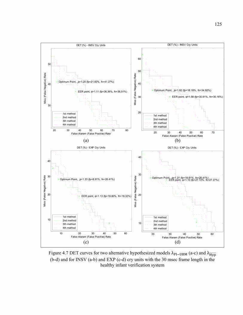
125
(a) (b)
(c) (d)
Figure 4.7 DET curves for two alternative hypothesized models λ (a-c) and λ
(b-d) and for INSV (a-b) and EXP (c-d) cry units with the 30 msec frame length in the healthy infant verification system
20 30 40 50 60 70 80
30
40
50
False Alaram (False Positive) Rate
Mis
s (F
alse
Neg
ativ
e) R
ate
DET (%) - INSV Cry Units
Optimum Point, ¸θ=1.20 (fp=21.82%, fn=41.27%)
EER point, θ=1.11 (fp=36.36%, fn=36.51%)
1st method
2nd method3th method
4th method
20 30 40 50 60 70
20
30
40
50
60
False Alaram (False Positive) RateM
iss
(Fal
se N
egat
ive)
Rat
e
DET (%) - INSV Cry Units
Optimum Point, ¸θ=1.82 (fp=18.18%, fn=34.92%)
EER point, θ=1.58 (fp=30.91%, fn=30.16%)
1st method
2nd method3th method
4th method
10 20 30 40 50 60
10
20
30
40
False Alaram (False Positive) Rate
Mis
s (F
alse
Neg
ativ
e) R
ate
DET (%) - EXP Cry Units
Optimum Point, ¸θ=1.33 (fp=8.91%, fn=28.41%)
EER point, θ=1.13 (fp=19.80%, fn=19.32%)
1st method
2nd method3th method
4th method
20 30 40 50 60
10
20
30
40
False Alaram (False Positive) Rate
Mis
s (F
alse
Neg
ativ
e) R
ate
DET (%) - EXP Cry Units
Optimum Point, ¸θ=1.21 (fp=18.81%, fn=28.41%) EER point, θ=1.10 (fp=27.72%, fn=27.27%)
1st method
2nd method3th method
4th method

126
All of the points on the DET curves have different (%) and (%), and in practice,
the operating point (OP) should be selected based on the task of the system in which all of
the application criteria are met. For example, in biometric security systems, the point must
have a low FAR. Because finding the best suitable OP in such a diagnostic system is not our
concern in this paper, the equal error rate (EER) points are plotted by individual circle-
shaped points on curves where ( ) = ( ), ∈ S, and S is the set of thresholds for
calculating the OP distribution. Note that an exact EER point might not exist. Moreover, the
optimal ROC operating points described in (Metz, 1978) are shown by the square-shaped
points on the curves. The decision threshold is selected in a way that minimizes the average
cost at this point. The slope of the ROC at this point is given by
S = C − CC − C × P(+D)P(−D) (4.16)
where C , C , C , C are the costs, and (∓ ) is equal to the probability that a case
from the database is an ∓ case.
Here, our predefined costs for computing are as follows:
= = 0.5, = = 0 (4.17)
The overall accuracy and error rates depend on the chosen operating point, which is not clear
here. Therefore, to compare the systems fairly and independently of the cutpoint, the Area
under the ROC curve (AUC) is used as a measure of the performance of the detector, while
an ideal classifier has an AUC equal to 1. The value of EER (%) and AUC for the systems
plotted in Figure 4.6 and Figure 4.7 are listed in Table 4.6. It is apparent that the experiments
on the shorter frame length have better results in most of the cases and the EXP cry units
have a more distinctive ability than the INSV cry units in classifying healthy and sick infants
independent of the frame length, as we anticipated. Moreover, because in general each cry
signal contains more EXP cry units than INSV cry units, the average LLR score computed
127
over EXP cry units is more reliable than the INSV units due to having a larger number of
available EXP units in the samples. To show the impact of the number of cry units on the
system performance, especially for the INSV type (the same as in Figure 4.5 except for the
values), we apply a criterion to choose only test files that have at least 3 cry units to perform
the classification.
Almost all of the cry test samples with EXP-labeled segments have more than 3 units except
for one healthy and two sick samples; therefore, the achieved results for the expiratory cry
units are the same as the results in Table 4.6 again. However, this condition has a larger
effect on the inspiratory segments of the recorded infants’ cry signals and reduces the number
of test files that contain INSV segments that have any duration (86 healthy and 93 sick to 32
healthy and 23 sick) cry samples. Independent of the frame length, adaptation method and
background model, the results given in Table 4.7confirm that there are more INSV cry units
inside a test file, with a higher chance at the end of the evaluation to diagnose it correctly.
Among the four adaptation methods defined earlier, our reference system with the Bayesian
or MAP adaptation method (method 1) has the lowest AUC, and the other specific methods,
both 2-3, which use the BML adaptation estimates, have lower error-detection rates with a
higher AUC. The system with the highest AUC for both the EXP and INSV cry units is the
system that uses the background model and the 2nd method of adaptation. Therefore, the
minimum achieved equal error rates are 14.85% and 25.8% for the EXP and INSV cry units,
respectively.

128
Table 4.6 Comparison of the different healthy infant detector systems based on the Equal error rate and Area under the curve for all of the test samples
INSV 10 msec 30 msec
EER (%) AUC EER (%) AUC
'method1' 29.03 27.41 0.77 0.806 41.81 38.18 0.62 0.68
'method2' 27.41 25.80 0.815 0.8350 36.36 30.90 0.69 0.77
'method3' 27.41 25.80 0.811 0.8355 38.18 29.09 0.68 0.81
'method4' 29.03 29.03 0.78 0.80 40 34.54 0.64 0.71
EXP 10 msec 30 msec
EER (%) AUC EER (%) AUC
'method1' 27.72 15.8415 0.81 0.932 20.79 32.67 0.87 0.76
'method2' 23.76 14.8514 0.84 0.951 19.80 27.72 0.89 0.825
'method3' 24.75 15.8415 0.826 0.951 22.77 24.75 0.86 0.824
'method4' 25.74 15.8415 0.827 0.932 18.81 30.69 0.89 0.77
Table 4.7 Comparison of the different healthy infant detector systems based on the EER and AUC for the test samples that have more than 3 INSV units (32 and 23 cry
samples of healthy and sick infants respectively)
INSV 10 msec 30 msec
EER (%) AUC EER (%) AUC
'method1' 13.043 26.08 0.933 0.872 25 25 0.75 0.81
'method2' 13.043 17.39 0.944 0.888 30 25 0.79 0.82
'method3' 13.043 21.73 0.941 0.887 35 25 0.77 0.85
'method4' 13.043 26.08 0.938 0.877 25 20 0.78 0.82
129
4.6.3.2 Sick infant detector with a specific disease
A lack of data, especially in the training data for a specific illness, causes difficulty in
training and adapting well-defined models, such as the INSV model type for infants who
have blood disorders. Even at the evaluation time, there are not a sufficient number of test
samples in all of the diseases (see Table 4.5). Thus far, we have only used our detector for
sick infants who suffer from neurological and respiratory disorders. In the interest of brevity,
only the results for a shorter frame length and background speaker models will be
discussed.
Recording sick infants’ cries that are available in the training CDB have been taken from a
limited number of distinct infants, which are not the same as for the infants used in the test
CDB. In total, 10 and 5 infants are used to train the respiratory and neurological disease
models, respectively. In comparison to previous results in the healthy infant detector system,
very low training errors plus test results for the unseen data depicted in Table 4.8 might be a
sign of memorizing training data rather than learning.
This finding is due to an apparent lack of enough distinct infants in each corresponding class,
especially for neurological disease. It is important to understand that the data collection
process, training and adapting procedures are time-consuming, but that also, in spite of them,
further corresponding full-term sick infants (as with healthy infants) result in better
generalization by training well-defined models. Even using cross-validation, which is a
method for preventing overfitting, is not a quick-fix solution. Therefore, collecting new data
to increase the size of the training CDB to rebuild a pathology-independent background
model and sickness models is a practical solution to improving the performance.
It has been shown in Table 4.8 that the methods that use BML adaptation, the 2nd, 3rd and 4th
methods, have the highest AUC than our reference system with Bayesian adaptation.
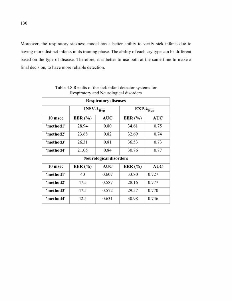
130
Moreover, the respiratory sickness model has a better ability to verify sick infants due to
having more distinct infants in its training phase. The ability of each cry type can be different
based on the type of disease. Therefore, it is better to use both at the same time to make a
final decision, to have more reliable detection.
Table 4.8 Results of the sick infant detector systems for Respiratory and Neurological disorders
Respiratory diseases
INSV- EXP-
10 msec EER (%) AUC EER (%) AUC
'method1' 28.94 0.80 34.61 0.75
'method2' 23.68 0.82 32.69 0.74
'method3' 26.31 0.81 36.53 0.73
'method4' 21.05 0.84 30.76 0.77
Neurological disorders
10 msec EER (%) AUC EER (%) AUC
'method1' 40 0.607 33.80 0.727
'method2' 47.5 0.587 28.16 0.777
'method3' 47.5 0.572 29.57 0.770
'method4' 42.5 0.631 30.98 0.746
131
4.6.4 Fusion, calibration and decision
A more sophisticated system can be developed by integrating the evidence presented by
multiple sources of information, similar to in multimodal biometric systems. Such a
multimodal system is expected to be more reliable in contrast to a unimodal system, which
relies on the evidence of a single source. Here, fusion of the proposed two subsystems
(expiratory and inspiratory cry unit-based GMM) is performed to improve the overall
performance. Generally speaking, the strategy of fusion can be categorized into three levels,
which are called the data or feature level, matching score level, and decision level (Blum et
Liu, 2005). Although the feature set is richer in discriminative information than the matching
score or the output decision of a classifier, fusion at the match score level is usually preferred
because it is relatively easy to obtain and there is no need to worry about the feature
compatibility at the score level or rigid fusion at the decision level (Ross et Jain, 2004).
There are two different strategies for combining scores that are generated by multiple
classifiers. In the first method, the final decision is made by a single scalar score that is a
combination of individual scores (Ben-Yacoub, Abdeljaoued et Mayoraz, 1999; Dieckmann,
Plankensteiner et Wagner, 1997). There are several techniques for addressing the
combination problem; these techniques can be applied in different applications (Li, Han et
Narayanan, 2013; Snelick et al., 2005). In the second approach, individual scores construct a
feature vector to verify or classify two classes (Vatsa, Singh et Noore, 2007; Verlinde et
Cholet, 1999). We took this approach to fuse the model scores that were obtained from the
expiratory and inspiratory cry units of the test samples.
As in multi-modal identity verification systems, we want to combine the output match scores
of two experts using the same features and arising from a specific measure, such as MFCCs
(static and dynamic) but also driven from different cry types. The normalized log-likelihood
ratio scores obtained from two EXP and INSV cry unit-based subsystems are concatenated to
construct a two-dimensional feature space. Then, we used three classification models, namely
the multilayer perceptron (MLP) using the back-propagation algorithm, probabilistic neural

132
networks (PNN) and a support vector machine (SVM) (see Table 4.9). These classifiers were
evaluated using test datasets (see Table 4.4) that included cry signals that contained clean
EXP and INSV labeled segments.
Table 4.9 Training parameters used in SVM, PNN and MLP
PNN Number of neurons in layer 1 : 161
First layer Transfer function : Radial basis transfer function
Spread value: 0.1
Number of neurons in layer 2 : 2
Second layer Transfer function : Competitive transfer function
Performance function : mse
Learning algorithm : Scaled conjugate gradient
MLP Number of hidden layers : 1
Hidden layer neurons : 10
Hidden activation function : Hyperbolic tangent sigmoid
Output layer neurons : 2
Output activation function : Softmax (normalized exponential)
Max number of iteration : 1000
Performance function : Crossentropy
Learning algorithm : Scaled conjugate gradient
SVM Number of iterations : 15000
Kernel functions :
1- linear
2- Quadratic
3- Polynomial (order 3)
4- Gaussian RBF Kernel
5- Multilayer perceptron Kernel with SMO method to find the
separating hyperplane
133
4.6.5 Results and discussion
To compare the generalizability of these three different algorithms and to find out the best
algorithm for the available data, stratified K-fold cross-validation is used in which each fold
has a roughly equal size and contains the same percentage of samples of each target class as
in the whole dataset. Although 10-fold cross-validation is more common, in practice, usually
the choice of the number of folds depends on the size of the dataset. Although there are
different variants of cross-validated estimates (Refaeilzadeh, Tang et Liu, 2009), stratified
10-fold cross-validation is recommended by Kohavi (Kohavi, 1995) as the best model.
To obtain reliable performance estimation, multiple rounds of cross-validation are performed
to test new and different random splits that result in smaller variance in the results and reduce
the variability. Then, the validation results with three different values of , depicted in Table
4.10, are averaged over the corresponding number of rounds.
Table 4.10 Number of folds and rounds
Value of K 3 5 10
Number of Iterations 400 200 100
The performances of the classifiers that use different adaptation methods are compared based
on some widely used statistical measures, namely, the false positive rate, false negative rate,
accuracy, sensitivity and specificity. These statistical measures can be calculated from the
classifier’s results, as described in (Fawcett, 2006). The error of the classifier follows a
binomial distribution with the following mean and standard deviation:
= , = ( )
(4.18)

134
where is the mean of errors, and n is the number of samples. We can approximate the 100(1 − )% confidence interval for the error by the Wald confidence interval (Agresti et
Coull, 1998), as follows:
∓ ⁄ (4.19)
where is the 1 − β quantile of the standard normal distribution. In Table 4.5, the test
dataset consists of 86 and 93 cry samples of healthy and sick infants whose recorded cry
signals contain both EXP and INSV segments, which are used to detect healthy infants by
fusing likelihood ratio scores obtained from expiratory and inspiratory cry units. In the first
experiment, the dataset is tested by the aforementioned classifiers (listed in Table 4.9), which
have different adaptation techniques that are used to train the subclass models, as described
in previous sections. Figure 4.8 indicates both types of errors, the false positive rate (FPR or
type I error) and the false negative rate (FNR or type II error), with an 80% confidence
interval after applying stratified K-fold cross-validation for each classifier. Due to space
limitations, we only plot the test errors over new observations (that were not used in the
training phase of the K-fold cross-validation) and not training errors over the observations
used in its training. For each method of adaptation (from methods 1-4), there is not much
difference in the errors between the K-fold cross-validations with different values of folds.
The Bayesian adaptation method (1st method), which is our reference method, has obviously
higher errors than the other methods, especially the 2nd and 3rd methods. To obtain a better
comparison between the performances of the adaptation methods, Table 4.11 depicts the
average accuracy, sensitivity and specificity rates over all of the used classifiers for each
adaptation method. Here, the accuracy rate indicates the proportion of true classified infants
(both healthy and sick) among the total number of infants in the test dataset. The sensitivity
measures the portion of healthy infants that are correctly identified, while the specificity
measures the proportion of sick infants that are correctly verified. As is clear, the BML
adaptation method for refining both the mean and variance vectors (2nd method) and the
coupled BML adaptation estimations with old estimations (3rd method) are superior to the
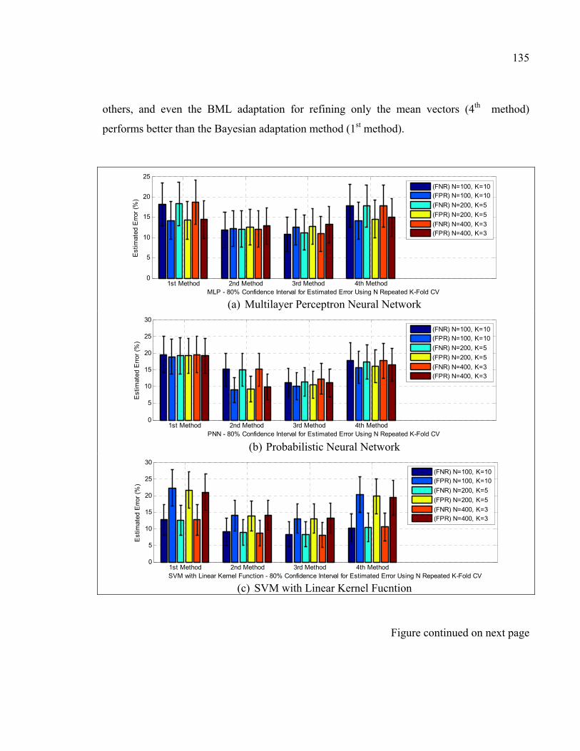
135
others, and even the BML adaptation for refining only the mean vectors (4th method)
performs better than the Bayesian adaptation method (1st method).
(a) Multilayer Perceptron Neural Network
(b) Probabilistic Neural Network
(c) SVM with Linear Kernel Fucntion
Figure continued on next page
1st Method 2nd Method 3rd Method 4th Method0
5
10
15
20
25
MLP - 80% Confidence Interval for Estimated Error Using N Repeated K-Fold CV
Est
imat
ed E
rror
(%
)
(FNR) N=100, K=10(FPR) N=100, K=10
(FNR) N=200, K=5
(FPR) N=200, K=5
(FNR) N=400, K=3(FPR) N=400, K=3
1st Method 2nd Method 3rd Method 4th Method0
5
10
15
20
25
30
PNN - 80% Confidence Interval for Estimated Error Using N Repeated K-Fold CV
Est
imat
ed E
rror
(%
)
(FNR) N=100, K=10(FPR) N=100, K=10
(FNR) N=200, K=5
(FPR) N=200, K=5
(FNR) N=400, K=3(FPR) N=400, K=3
1st Method 2nd Method 3rd Method 4th Method0
5
10
15
20
25
30
SVM with Linear Kernel Function - 80% Confidence Interval for Estimated Error Using N Repeated K-Fold CV
Est
imat
ed E
rror
(%
)
(FNR) N=100, K=10(FPR) N=100, K=10
(FNR) N=200, K=5
(FPR) N=200, K=5
(FNR) N=400, K=3(FPR) N=400, K=3
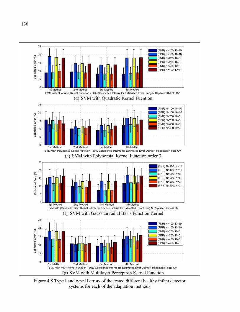
136
(d) SVM with Quadratic Kernel Fucntion
(e) SVM with Polynomial Kernel Function order 3
(f) SVM with Gaussian radial Basis Function Kernel
(g) SVM with Multilayer Perceptron Kernel Function
Figure 4.8 Type I and type II errors of the tested different healthy infant detector systems for each of the adaptation methods
1st Method 2nd Method 3rd Method 4th Method0
5
10
15
20
25
SVM with Quadratic Kernel Function - 80% Confidence Interval for Estimated Error Using N Repeated K-Fold CV
Est
imat
ed E
rror
(%
)
(FNR) N=100, K=10(FPR) N=100, K=10
(FNR) N=200, K=5
(FPR) N=200, K=5
(FNR) N=400, K=3(FPR) N=400, K=3
1st Method 2nd Method 3rd Method 4th Method0
5
10
15
20
25
SVM with Polynomial Kernel Function - 80% Confidence Interval for Estimated Error Using N Repeated K-Fold CV
Est
imat
ed E
rror
(%
)
(FNR) N=100, K=10(FPR) N=100, K=10
(FNR) N=200, K=5
(FPR) N=200, K=5
(FNR) N=400, K=3(FPR) N=400, K=3
1st Method 2nd Method 3rd Method 4th Method0
5
10
15
20
25
SVM with (Gaussian) RBF Kernel - 80% Confidence Interval for Estimated Error Using N Repeated K-Fold CV
Est
imat
ed E
rror
(%
)
(FNR) N=100, K=10(FPR) N=100, K=10
(FNR) N=200, K=5
(FPR) N=200, K=5
(FNR) N=400, K=3(FPR) N=400, K=3
1st Method 2nd Method 3rd Method 4th Method0
5
10
15
20
25
SVM with MLP Kernel Function - 80% Confidence Interval for Estimated Error Using N Repeated K-Fold CV
Est
imat
ed E
rror
(%
)
(FNR) N=100, K=10(FPR) N=100, K=10
(FNR) N=200, K=5
(FPR) N=200, K=5
(FNR) N=400, K=3(FPR) N=400, K=3
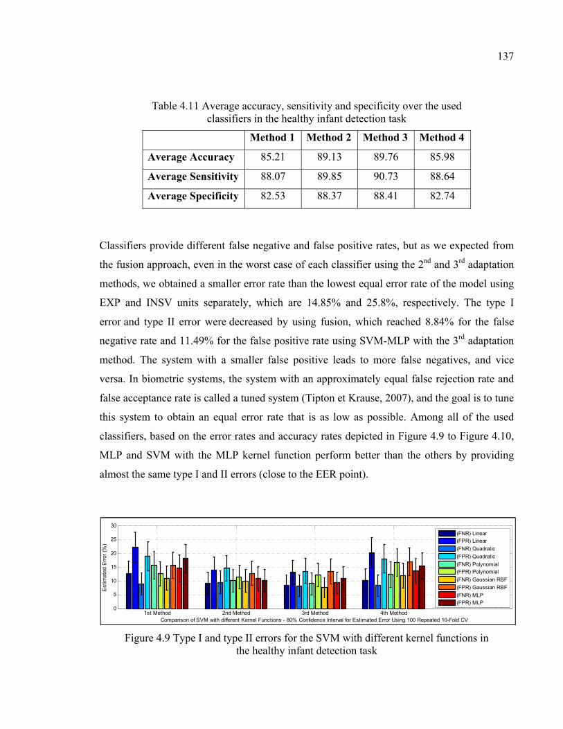
137
Table 4.11 Average accuracy, sensitivity and specificity over the used classifiers in the healthy infant detection task
Method 1 Method 2 Method 3 Method 4
Average Accuracy 85.21 89.13 89.76 85.98
Average Sensitivity 88.07 89.85 90.73 88.64
Average Specificity 82.53 88.37 88.41 82.74
Classifiers provide different false negative and false positive rates, but as we expected from
the fusion approach, even in the worst case of each classifier using the 2nd and 3rd adaptation
methods, we obtained a smaller error rate than the lowest equal error rate of the model using
EXP and INSV units separately, which are 14.85% and 25.8%, respectively. The type I
error and type II error were decreased by using fusion, which reached 8.84% for the false
negative rate and 11.49% for the false positive rate using SVM-MLP with the 3rd adaptation
method. The system with a smaller false positive leads to more false negatives, and vice
versa. In biometric systems, the system with an approximately equal false rejection rate and
false acceptance rate is called a tuned system (Tipton et Krause, 2007), and the goal is to tune
this system to obtain an equal error rate that is as low as possible. Among all of the used
classifiers, based on the error rates and accuracy rates depicted in Figure 4.9 to Figure 4.10,
MLP and SVM with the MLP kernel function perform better than the others by providing
almost the same type I and II errors (close to the EER point).
Figure 4.9 Type I and type II errors for the SVM with different kernel functions in the healthy infant detection task
1st Method 2nd Method 3rd Method 4th Method0
5
10
15
20
25
30
Comparison of SVM with different Kernel Functions - 80% Confidence Interval for Estimated Error Using 100 Repeated 10-Fold CV
Est
imat
ed E
rror
(%
)
(FNR) Linear(FPR) Linear
(FNR) Quadratic
(FPR) Quadratic
(FNR) Polynomial(FPR) Polynomial
(FNR) Gaussian RBF
(FPR) Gaussian RBF
(FNR) MLP(FPR) MLP
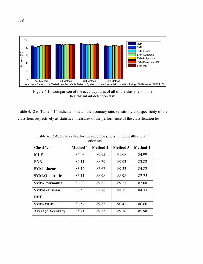
138
Figure 4.10 Comparison of the accuracy rates of all of the classifiers in the healthy infant detection task
Table 4.12 to Table 4.14 indicate in detail the accuracy rate, sensitivity and specificity of the
classifiers respectively as statistical measures of the performance of the classification test.
Table 4.12 Accuracy rates for the used classifiers in the healthy infant detection task
Classifier Method 1 Method 2 Method 3 Method 4
MLP 85.03 89.95 91.68 84.99
PNN 82.11 88.79 89.93 83.82
SVM-Linear 83.12 87.67 89.33 84.82
SVM-Quadratic 86.11 88.98 88.98 87.25
SVM-Polynomial 86.99 89.82 89.27 87.08
SVM-Gaussian
RBF
86.59 88.78 88.75 84.33
SVM-MLP 86.57 89.85 90.41 86.60
Average Accuracy 85.21 89.13 89.76 85.98
1st Method 2nd Method 3rd Method 4th Method0
20
40
60
80
100
Accuracy Rates of the Tested Healthy Infants Detecor Systems for each Adaptation method Using 100 Repeated 10-Fold CV
Acc
urac
y (%
)
MLPPNN
SVM-Linear
SVM-Quadratic
SVM-Polynomial
SVM-Gaussian RBFSVM-MLP
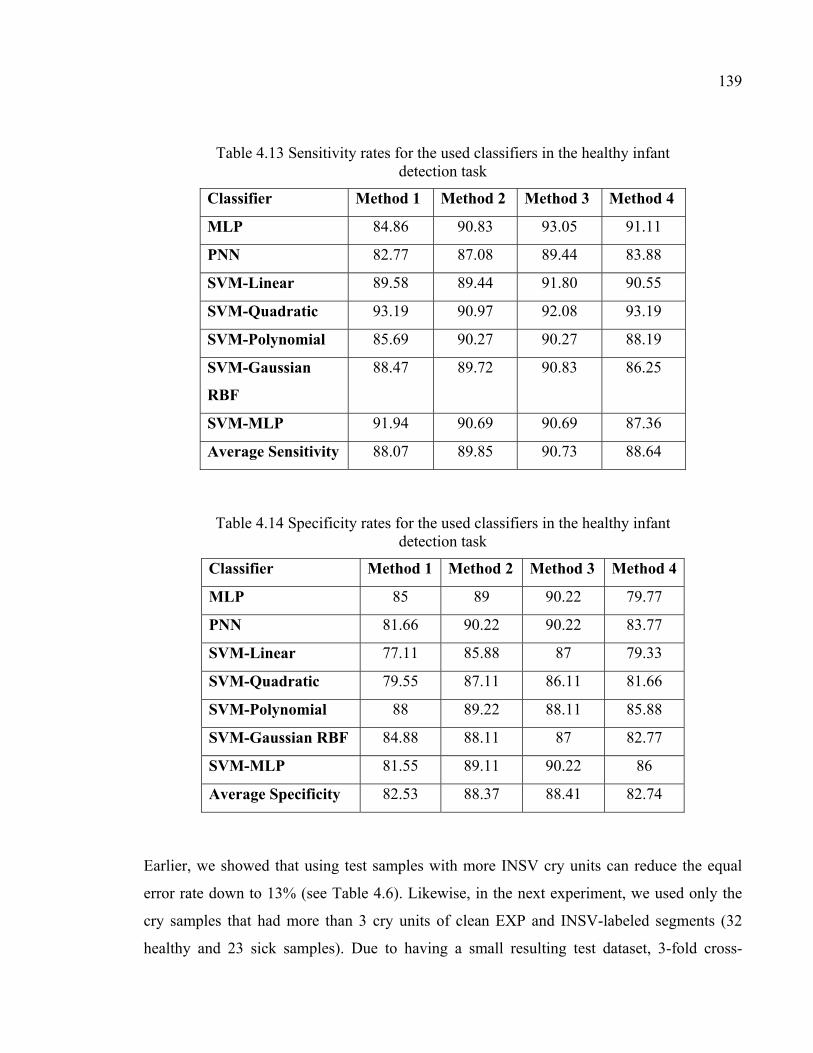
139
Table 4.13 Sensitivity rates for the used classifiers in the healthy infant detection task
Classifier Method 1 Method 2 Method 3 Method 4
MLP 84.86 90.83 93.05 91.11
PNN 82.77 87.08 89.44 83.88
SVM-Linear 89.58 89.44 91.80 90.55
SVM-Quadratic 93.19 90.97 92.08 93.19
SVM-Polynomial 85.69 90.27 90.27 88.19
SVM-Gaussian
RBF
88.47 89.72 90.83 86.25
SVM-MLP 91.94 90.69 90.69 87.36
Average Sensitivity 88.07 89.85 90.73 88.64
Table 4.14 Specificity rates for the used classifiers in the healthy infant detection task
Classifier Method 1 Method 2 Method 3 Method 4
MLP 85 89 90.22 79.77
PNN 81.66 90.22 90.22 83.77
SVM-Linear 77.11 85.88 87 79.33
SVM-Quadratic 79.55 87.11 86.11 81.66
SVM-Polynomial 88 89.22 88.11 85.88
SVM-Gaussian RBF 84.88 88.11 87 82.77
SVM-MLP 81.55 89.11 90.22 86
Average Specificity 82.53 88.37 88.41 82.74
Earlier, we showed that using test samples with more INSV cry units can reduce the equal
error rate down to 13% (see Table 4.6). Likewise, in the next experiment, we used only the
cry samples that had more than 3 cry units of clean EXP and INSV-labeled segments (32
healthy and 23 sick samples). Due to having a small resulting test dataset, 3-fold cross-
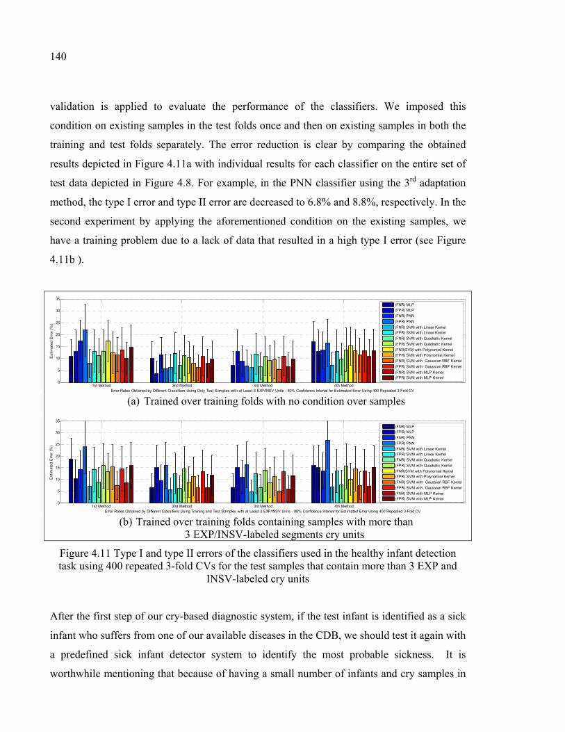
140
validation is applied to evaluate the performance of the classifiers. We imposed this
condition on existing samples in the test folds once and then on existing samples in both the
training and test folds separately. The error reduction is clear by comparing the obtained
results depicted in Figure 4.11a with individual results for each classifier on the entire set of
test data depicted in Figure 4.8. For example, in the PNN classifier using the 3rd adaptation
method, the type I error and type II error are decreased to 6.8% and 8.8%, respectively. In the
second experiment by applying the aforementioned condition on the existing samples, we
have a training problem due to a lack of data that resulted in a high type I error (see Figure
4.11b ).
(a) Trained over training folds with no condition over samples
(b) Trained over training folds containing samples with more than 3 EXP/INSV-labeled segments cry units
Figure 4.11 Type I and type II errors of the classifiers used in the healthy infant detection task using 400 repeated 3-fold CVs for the test samples that contain more than 3 EXP and
INSV-labeled cry units
After the first step of our cry-based diagnostic system, if the test infant is identified as a sick
infant who suffers from one of our available diseases in the CDB, we should test it again with
a predefined sick infant detector system to identify the most probable sickness. It is
worthwhile mentioning that because of having a small number of infants and cry samples in
1st Method 2nd Method 3rd Method 4th Method0
5
10
15
20
25
30
35
Error Rates Obtained by Different Classifiers Using Only Test Samples with at Least 3 EXP/INSV Units - 80% Confidence Interval for Estimated Error Using 400 Repeated 3-Fold CV
Est
imat
ed E
rror
(%
)
(FNR) MLP(FPR) MLP
(FNR) PNN
(FPR) PNN
(FNR) SVM with Linear Kernel(FPR) SVM with Linear Kernel
(FNR) SVM with Quadratic Kernel
(FPR) SVM with Quadratic Kernel
(FNR)SVM with Polynomial Kernel(FPR) SVM with Polynomial Kernel
(FNR) SVM with Gaussian RBF Kernel
(FPR) SVM with Gaussian RBF Kernel
(FNR) SVM with MLP Kernel(FPR) SVM with MLP Kernel
1st Method 2nd Method 3rd Method 4th Method0
5
10
15
20
25
30
35
Error Rates Obtained by Different Classifiers Using Training and Test Samples with at Least 3 EXP/INSV Units - 80% Confidence Interval for Estimated Error Using 400 Repeated 3-Fold CV
Est
imat
ed E
rror
(%
)
(FNR) MLP(FPR) MLP
(FNR) PNN
(FPR) PNN
(FNR) SVM with Linear Kernel(FPR) SVM with Linear Kernel
(FNR) SVM with Quadratic Kernel
(FPR) SVM with Quadratic Kernel
(FNR)SVM with Polynomial Kernel(FPR) SVM with Polynomial Kernel
(FNR) SVM with Gaussian RBF Kernel
(FPR) SVM with Gaussian RBF Kernel
(FNR) SVM with MLP Kernel(FPR) SVM with MLP Kernel
141
our CDB at this time, the GMMs were adapted from the corresponding pathology-
independent UBM for only infants who suffer from neurological problems and respiratory
disorders. Likewise, the classifiers listed in Table 4.9 were used to fuse the likelihood ratio
scores that were obtained from the expiratory and inspiratory cry units. For this purpose, all
of the cry samples that were recorded from sick infants that have both expiratory and
inspiratory segments, as depicted in Table 4.5, were used to test these two sick infant detector
systems. The stratified K-fold cross-validation estimates the prediction error in each task to
make an assessment of different adaptation methods.
In the test dataset, we have 29 and 45 cry samples recorded from sick infants who suffer from
neurological and respiratory disorders, respectively. For the first task, we had an imbalanced
dataset (29 target and 64 non-target cry samples), and there are a few ways to address this
problem; these approaches can be divided into data and algorithmic levels (Han, Wang et
Mao, 2005). Because the dataset was small, the idea of under-sampling or data reduction
techniques that remove only a majority of class samples is not an ideal solution. Another
approach is to apply a higher misclassification cost to the minority class. This approach can
balance out our imbalanced dataset, but here we assumed equal costs for the two types of
error. Consequently, we simply increased the size of our minority class (target class) by
duplicating the data. Although it was reported in (Kolcz, Chowdhury et Alspector, 2003) that
usually duplicating samples in a dataset has a detrimental effect on the model and accuracy
rate, many re-sampling methods (Han, Wang et Mao, 2005) have been proposed in data
mining algorithms as a solution to imbalanced data sets. Here, simple random over-sampling
has been performed to balance the data set through duplicating some random samples of the
minority class. It was observed that smaller error rates resulted for the created balanced data
set. Figure 4.12 indicates the type I and type II errors of the classifiers in the sick infant
(those affected by neurological problems) detection task for the balanced data set. For the
sake of brevity, we have illustrated only the error rates of the classifier using 100 repeated
10-fold cross-validation in these two sick infant detection tasks. As depicted in Figure 4.13,
almost all of the classifiers in this task that were adapted by either the 2nd or 3rd methods have
higher accuracy rates, except for PNN, which has low false negative and false positive error
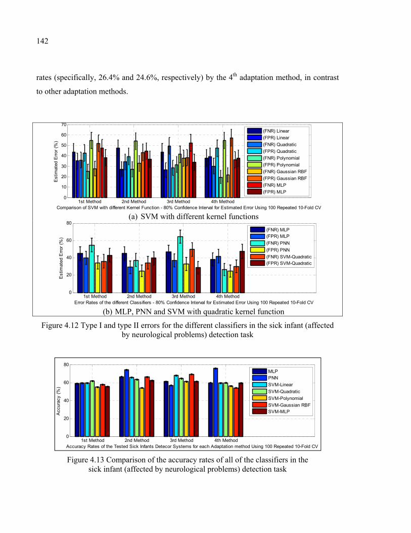
142
rates (specifically, 26.4% and 24.6%, respectively) by the 4th adaptation method, in contrast
to other adaptation methods.
(a) SVM with different kernel functions
(b) MLP, PNN and SVM with quadratic kernel function
Figure 4.12 Type I and type II errors for the different classifiers in the sick infant (affected by neurological problems) detection task
Figure 4.13 Comparison of the accuracy rates of all of the classifiers in the sick infant (affected by neurological problems) detection task
1st Method 2nd Method 3rd Method 4th Method0
10
20
30
40
50
60
70
Comparison of SVM with different Kernel Function - 80% Confidence Interval for Estimated Error Using 100 Repeated 10-Fold CV
Est
imat
ed E
rror
(%
)
(FNR) Linear
(FPR) Linear
(FNR) Quadratic
(FPR) Quadratic
(FNR) Polynomial
(FPR) Polynomial
(FNR) Gaussian RBF
(FPR) Gaussian RBF
(FNR) MLP
(FPR) MLP
1st Method 2nd Method 3rd Method 4th Method0
20
40
60
80
Error Rates of the different Classifiers - 80% Confidence Interval for Estimated Error Using 100 Repeated 10-Fold CV
Est
imat
ed E
rror
(%
)
(FNR) MLP(FPR) MLP
(FNR) PNN
(FPR) PNN
(FNR) SVM-Quadratic(FPR) SVM-Quadratic
1st Method 2nd Method 3rd Method 4th Method0
20
40
60
80
Accuracy Rates of the Tested Sick Infants Detecor Systems for each Adaptation method Using 100 Repeated 10-Fold CV
Acc
urac
y (%
)
MLPPNN
SVM-Linear
SVM-Quadratic
SVM-Polynomial
SVM-Gaussian RBFSVM-MLP
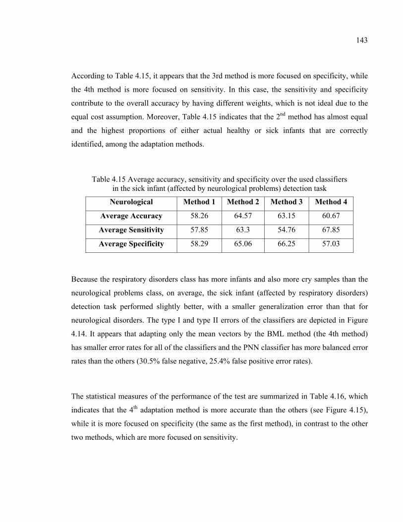
143
According to Table 4.15, it appears that the 3rd method is more focused on specificity, while
the 4th method is more focused on sensitivity. In this case, the sensitivity and specificity
contribute to the overall accuracy by having different weights, which is not ideal due to the
equal cost assumption. Moreover, Table 4.15 indicates that the 2nd method has almost equal
and the highest proportions of either actual healthy or sick infants that are correctly
identified, among the adaptation methods.
Table 4.15 Average accuracy, sensitivity and specificity over the used classifiers in the sick infant (affected by neurological problems) detection task
Neurological Method 1 Method 2 Method 3 Method 4
Average Accuracy 58.26 64.57 63.15 60.67
Average Sensitivity 57.85 63.3 54.76 67.85
Average Specificity 58.29 65.06 66.25 57.03
Because the respiratory disorders class has more infants and also more cry samples than the
neurological problems class, on average, the sick infant (affected by respiratory disorders)
detection task performed slightly better, with a smaller generalization error than that for
neurological disorders. The type I and type II errors of the classifiers are depicted in Figure
4.14. It appears that adapting only the mean vectors by the BML method (the 4th method)
has smaller error rates for all of the classifiers and the PNN classifier has more balanced error
rates than the others (30.5% false negative, 25.4% false positive error rates).
The statistical measures of the performance of the test are summarized in Table 4.16, which
indicates that the 4th adaptation method is more accurate than the others (see Figure 4.15),
while it is more focused on specificity (the same as the first method), in contrast to the other
two methods, which are more focused on sensitivity.
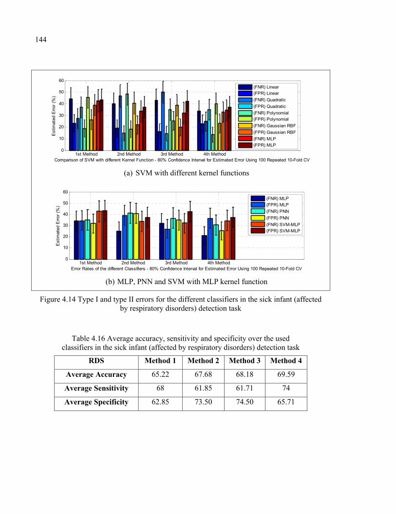
144
(a) SVM with different kernel functions
(b) MLP, PNN and SVM with MLP kernel function
Figure 4.14 Type I and type II errors for the different classifiers in the sick infant (affected by respiratory disorders) detection task
Table 4.16 Average accuracy, sensitivity and specificity over the used classifiers in the sick infant (affected by respiratory disorders) detection task
RDS Method 1 Method 2 Method 3 Method 4
Average Accuracy 65.22 67.68 68.18 69.59
Average Sensitivity 68 61.85 61.71 74
Average Specificity 62.85 73.50 74.50 65.71
1st Method 2nd Method 3rd Method 4th Method0
10
20
30
40
50
60
Comparison of SVM with different Kernel Function - 80% Confidence Interval for Estimated Error Using 100 Repeated 10-Fold CV
Est
imat
ed E
rror
(%
)
(FNR) Linear(FPR) Linear
(FNR) Quadratic
(FPR) Quadratic
(FNR) Polynomial(FPR) Polynomial
(FNR) Gaussian RBF
(FPR) Gaussian RBF
(FNR) MLP(FPR) MLP
1st Method 2nd Method 3rd Method 4th Method0
10
20
30
40
50
60
Error Rates of the different Classifiers - 80% Confidence Interval for Estimated Error Using 100 Repeated 10-Fold CV
Est
imat
ed E
rror
(%
)
(FNR) MLP(FPR) MLP
(FNR) PNN
(FPR) PNN
(FNR) SVM-MLP(FPR) SVM-MLP
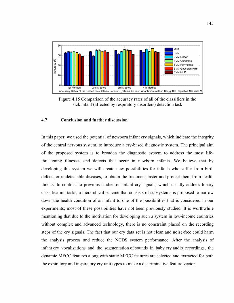
145
Figure 4.15 Comparison of the accuracy rates of all of the classifiers in the sick infant (affected by respiratory disorders) detection task
4.7 Conclusion and further discussion
In this paper, we used the potential of newborn infant cry signals, which indicate the integrity
of the central nervous system, to introduce a cry-based diagnostic system. The principal aim
of the proposed system is to broaden the diagnostic system to address the most life-
threatening illnesses and defects that occur in newborn infants. We believe that by
developing this system we will create new possibilities for infants who suffer from birth
defects or undetectable diseases, to obtain the treatment faster and protect them from health
threats. In contrast to previous studies on infant cry signals, which usually address binary
classification tasks, a hierarchical scheme that consists of subsystems is proposed to narrow
down the health condition of an infant to one of the possibilities that is considered in our
experiments; most of these possibilities have not been previously studied. It is worthwhile
mentioning that due to the motivation for developing such a system in low-income countries
without complex and advanced technology, there is no constraint placed on the recording
steps of the cry signals. The fact that our cry data set is not clean and noise-free could harm
the analysis process and reduce the NCDS system performance. After the analysis of
infant cry vocalizations and the segmentation of sounds in baby cry audio recordings, the
dynamic MFCC features along with static MFCC features are selected and extracted for both
the expiratory and inspiratory cry unit types to make a discriminative feature vector.
1st Method 2nd Method 3rd Method 4th Method0
20
40
60
80
Accuracy Rates of the Tested Sick Infants Detecor Systems for each Adaptation method Using 100 Repeated 10-Fold CV
Acc
urac
y (%
)
MLPPNN
SVM-Linear
SVM-Quadratic
SVM-Polynomial
SVM-Gaussian RBFSVM-MLP
146
Here, in our infant health-condition verification/detection system, the UBM is an infant-
independent GMM that is trained with cry samples from our cry dataset based on the HTK
(Hidden Markov Model Toolkit) software tool to represent the general acoustic
characteristics of crying. Then, for healthy or sick infants with an enrolled disease, a unique
cry-pattern has been trained by the adaptation procedure. In our previous papers (Farsaie
Alaie et Tadj, 2012; 2013), we showed that the BML method, compared to other learning
mixture models, has the great advantage of adding new mixture components in such a way
that the greatest improvement is obtained in the predefined objective function. We used this
idea to present a novel adapted BML process to derive subclass models from the GMM-
UBM. The Bayesian adaptation method is assumed here to be our reference system for the
adaptation procedure. The paper compares the obtained results for Bayesian and three
different variants of adapted BML methods on each classification task.
Both expiratory and inspiratory cry unit types have their own ability to classify test infants
for each task, and therefore, a score level fusion of the proposed two subsystems is
performed to make a more reliable decision. In brief, the system for each model has two main
sequential steps, which are called encoding and making a decision. In the encoding stage, we
show how a cry signal represents itself in both the expiration and inspiration cry units within
the GMM models by a set of extracted MFCC feature vectors and how to create log-
likelihood ratio scores. At the score level, the detection decision on each test infant’s cry is
based on whether the set of feature vectors observed on the presented cry signal is more
likely to have been produced by the hypothesized health-condition class or by the other
available alternative classes. In the next step, the fusion of the obtained individual scores is
performed to construct a new feature vector. The efficiency of the various classifiers, such as
SVM, MLP, and PNN, has been evaluated to compare the adaptation methods in each task.
Two health-independent and pathology-independent GMMs were trained by pooling the
corresponding training data in a balanced version of CDB together (39 healthy, 22 sick), and
we used the remainder of the unseen infant recordings in CDB for adapting the subclass
147
models. Then, testing was performed on all of the unseen 42 healthy and 40 sick infants, to
evaluate the accuracy of each model. The results indicated that independent of the type of the
cry units (EXP/INSV), adaptation method and task of the detector, the experiments on a
shorter frame length (10 msec) have lower equal error rates (EER) than the 30 msec frame
length in most of the cases. Moreover, based on the obtained results, the Bayesian or MAP
adaptation method (1st method) not only has a higher EER but also has a lower AUC than the
other three variants of the adapted BML method. In the first task, which was designed to
detect healthy infants from sick infants who suffer from specific diseases according to the
optimal likelihood ratio test, 14.85% and 25.8% equal error rates were achieved for the EXP
and INSV cry units, respectively. This finding indicates that there is a higher ability for
expiratory sounds to distinguish healthy and sick full-term infants in contrast to a sick infant
detector for respiratory disorders, while the trained model based on inspiratory sounds has a
lower error rate than those based on expiratory sounds.
Although the presence of noise in the database has caused a loss of some portion of the INSV
and EXP sounds in the baby cry audio recordings, the fact that the duration of the expiratory
sounds is usually larger than the inspiratory sounds in newborn infant cries makes the
average LLR score computed over expiratory cry units a more reliable estimate of
the true value than the inspiratory cry units. We have shown that the length of the expiratory
or inspiratory sounds that are available in a test file has a direct effect on the classification
performance. In other words, the more information that is available (the EXP/INSV length
inside each file), the more likely it is to have a more reliable decision and less uncertainty
about the detected pathological condition. Those infants whose sample cries do not contain
sufficient evidence should be asked to provide more samples. We concluded from the results
on the healthy infant and sick infant (with neurological and respiratory disorders) that the
ability of each cry type can vary by the type of disease or the general health condition.
Afterward, the obtained scores for each cry sample were used to construct a feature vector to
combine expiratory and inspiratory cry-based individual scores. Several classifiers have been
148
employed to evaluate the performance of the methods of adapting healthy and pathological
subclasses after the score level fusion. The error rates dropped from EER = 14.85%andEER = 25.8% in the healthy infant detector systems to an
8.84% false negative rate and 11.49% false positive rate using SVM-MLP with a variant of
the BML adaptation method. Likewise, the error rates in sick infant (with neurological and
respiratory disorders) detector systems were decreased by using score level fusion, and they
even reached a 26.4% false negative and 24.6% false positive error rate and a 30.5% false
negative and 25.4% false positive error rate using the PNN classifier with a variant of the
BML adaptation method (4th method) on each task, respectively. Overall, the 2nd and 3rd
adaptation methods, which use both the mean and variance vectors of the BML adaptation
estimates, have almost the highest accuracy, sensitivity and specificity among the adaptation
methods. The poor performance of the disease models (especially for infants with
neurological disorders) in comparison to healthy or sick infant models is largely due to
having a limited number of infants and also a lack of corresponding cry recordings.
Consequently, the trained GMMs with corresponding cry samples were not defined as well as
the healthy or sick models were when representing the general cry characteristics of the
enrolled diseases.
4.8 Acknowledgment
The authors would like to thank Dr. Barrington and members of the neonatology group of
Mother and Child University Hospital Center in Montreal (QC) for their dedication to the
collection of the Infant cry data base. This research has been funded by a grant from the Bill
& Melinda Gates Foundation through the Grand Challenges Explorations Initiative.
CONCLUSION
This thesis is conceived as a research work of MMS laboratory of Université du Québec,
École de technologie supérieure under the direct supervision of Dr. Chakib Tadj.
The ambitious goal – the non-invasive newborn cry-based diagnostic system – is design of an
additional tool or health care system that can be trained to work as an indispensable assistant
to help the pediatricians who have misgivings arrive at a decision. The system would be able
to classify healthy and sick infants who suffer from different enrolled diseases or
pathological conditions. If you break down this goal into smaller steps, in this thesis we
reached a significant milestone one the way to the newborn cry-based diagnostic system.
Most of the previous works on assessment of infant cry provide a binary classification of
healthy infants from sick infants who suffer from a known (specific) disease such as deaf
babies. Nonetheless, in this work the focus of attention in the domain is shifted into the open-
set multi-pathology recognition scenario. In other words, there is a class called “others” or
“none-of-the-above” in the target set dedicated solely to the test sick infants who suffer from
unseen out-of-set sicknesses that are not enrolled in the system yet. Therefore, an informed
choice of pathological states and collecting of the infant cry data base were necessary and
unavoidable which have been done in the neonatology departments of several hospitals in
Canada and Lebanon. It is worth mentioning that due to the inspiration behind this research
work, there was no constraint placed on the recording procedure of infant cry signals.
Our work employed Gaussian Mixture Models (GMMs) as a flexible and powerful
probabilistic tool for modeling multivariate stochastic feature vectors extracted from infant
cry signals. Our basic goal in learning GMM is to estimate the unknown parameters of
Gaussian mixture distributions that the extracted cry features are hypothetically come from.
Adapted BML method was introduced in this work to learn growing GMM in an incremental
and recursive manner. We have shown that not only the value of the log-likelihood for GMM
trained with adapted BML method bears a close resemblance to that of GMM trained with
150
the traditional EM algorithm, but using this method has some benefits such as adding a new
component to the direction that increase the predefined objective function the most, reducing
sensitivity to initial parameters and estimating the optimum number of components based on
incremental manner.
In data preprocessing, including selection and extraction of pathologically-informed features,
different frame lengths (10-30 mec) with the same overlap percentage between two
consecutive windows were considered for short-term processing of infant cry signals. The
well-known acoustic features of speech, the dynamic MFCC features along with static
MFCC features, have been extracted from both manually segmented expiratory and
inspiratory infant cry vocalizations separately in this study. The results indicated that
independent of the type of the cry units, adaptation method and classification task, the
experiments on a shorter frame length have lower error rates in most of the cases.
We also brought the Gaussian Mixture Model - Universal Background Model (UBM)
framework which is widely used in speaker recognition and verification domains, into
newborn cry-based pathology recognition. Two health-independent and pathology-
independent GMM-UBMs with a large number of mixture components were trained from a
large amount of cry uttered by lots of full-term healthy and sick infants to represent the
general cry feature characteristics for each population. Due to limitation of training infant cry
data from an enrolled pathological condition, a target pathology model is derived from
adapting the parameters of UBM using the infants’ enrollment cries. A variant of boosted
mixture learning (BML) method is employed in order to derive a unique cry-pattern for each
enrolled disease from the GMM-UBM by adaptation of GMM parameters. We have shown
how this boosting-based approach can also enhance maximum a-posterior (MAP) or
Bayesian adaptation of the parameters of GMM-UBM. Note that the traditional EM
algorithm and MAP adaptation method are assumed to be our reference systems in the GMM
training process and adaptation of GMM in this work.
151
In our investigation into short-time power spectrum of cry signals, we found that more than
94% of the energy in typical healthy and sick infant cry signals is stored within less than 4
kHz of bandwidth. However, the results indicates that the energies of the inspiration cry
vocalizations for sick infants tend to accumulate at a slower rate than the energies of the
expiration segments, especially in cases of RDS disorders. Moreover, since in typical infant
cry signals inspiration is much shorter than expiration and therefore the average likelihood
ratio over expiration cry units is more reliable than inspiration cry units. As a result of above-
mentioned differences in the types of cry sounds, expiration–based models have more
distinctive abilities than inspiration-based models in classifying healthy and sick infants
independent of the frame length.
The detection decision on each test infant’s cry is based on whether the set of feature vectors
observed on the presented cry signal is more likely to have been produced by the
hypothesized health-condition class or by the other available alternative classes. In the next
step, individual scores for both types of cry sounds construct a new feature vector in order to
make a score level fusion. The results of experiments confirm that this approach is able to
provide valuable information that comes from the fusion of the proposed two independent
subsystems to a more reliable decision making process.
In fact, we have achieved what we have aimed for in our objective and accordingly have
contributed in advancement of the algorithm for learning statistical Gaussian mixture models.
Moreover, Maximum a-Posterior (MAP) adaptation of the parameters of the GMM-UBM is
enhanced with the implementation of ideas used for boosted mixture learning method. In
brief, the proposed diagnostic system depicted in Figure 4.16 is built around the likelihood
ratio test by using GMMs for likelihood functions and GMM-UBM models to derive
subclass models from the related UBM via the adapted-BML method instead of common
Bayesian adaptation.
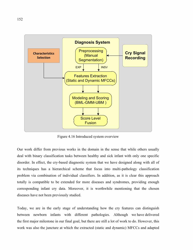
152
Characteristics Selection
EXP
Modeling and Scoring(BML-GMM-UBM )
Diagnosis System
Preprocessing(Manual
Segmentation)
Features Extraction(Static and Dynamic MFCCs)
Cry Signal Recording
Score Level Fusion
EXP INSV
Figure 4.16 Introduced system overview
Our work differ from previous works in the domain in the sense that while others usually
deal with binary classification tasks between healthy and sick infant with only one specific
disorder. In effect, the cry-based diagnostic system that we have designed along with all of
its techniques has a hierarchical scheme that focus into multi-pathology classification
problem via combination of individual classifiers. In addition, as it is clear this approach
totally is compatible to be extended for more diseases and syndromes, providing enough
corresponding infant cry data. Moreover, it is worthwhile mentioning that the chosen
diseases have not been previously studied.
Today, we are in the early stage of understanding how the cry features can distinguish
between newborn infants with different pathologies. Although we have delivered
the first major milestone in our final goal, but there are still a lot of work to do. However, this
work was also the juncture at which the extracted (static and dynamic) MFCCs and adapted
153
boosted mixture learning method gathered around the Gaussian mixture models to help us to
gradually get closer to our goal. Despite the main limitation of the current work stated in
content which is small cry database corpus, in the 2nd and 3rd chapters we showed the ability
of GMMs to create cry patterns for healthy and sick infants by using static MFCCs.
Afterward, in the 4th chapter, some experiments that investigate the ability of both expiratory
and inspiratory cry vocalizations separately were described. Moreover, due to lack of cry
corpus for sick infants especially with some specific diseases, we tried to categorize diseases
based on the grouping of symptoms and organs affected. Consequently, in each of five new
categories we had more data to train Gaussian models. Procedure of collecting infant cry data
base is still in progress but so far it is not enough to create a universal background model for
infant cry signals due to small number of infants in each category. Consequently,
we still have a long way to go and more research must be done to ensure that the system is
practical and reliable.

RECOMENDATIONS
Some directions for future research related to current study are proposed in the following:
Humans use several levels of information to recognize the reason behind the babies’ cry, but
automatic systems are still dependent on the low-level acoustic information. The challenges
in this area are to find, reliably extract, and effectively use these higher levels of information
from the cry signal. It is likely that these higher levels of information will not provide good
performance on their own and may need to be fused with more acoustic-based systems.
Techniques to fuse and apply high-level information with low-level acoustic features need to
be developed in a way that makes the feature classes work synergistically.
Same as multi-modal identity verification systems, combination of the output score of
different experts using different and independent cry feature characteristics such as MFCCs,
MFDWC, fundamental frequency and formants can represent a remarkable achievement in
the domain. We recommend testing the performance of the diagnostic system using a fuzzy
classifier to classify and identify different pathological cries. This classifier uses fuzzy logic
to model and classify the different cries. Fuzzy logic rule can be defined for each kind of
pathology to describe the relationship between the features and pathological condition. The
time-domain and frequency-domain pathological cries characterization presented in this work
such as (hyper-phonic and dysphonic segments, the irregularity of fundamental frequency)
might enhance the performance of the diagnostic system. We also recommend the merger of
the two classifiers (GMM classifier and fuzzy).
In human speech signals there is not much information above 6.8 kHz. It has been shown in
this work that cry signals of full-term healthy and sick infants have more than 94% of their
energies below 4 kHz. So far, information up to 4 kHz bandwidth of recorded infant cry
signals has been used and therefore, the idea of band splitting and sub-band features on the
upper frequency band might be worthwhile to try in order to make sure that there is no loss of
information.
156
As we discussed it earlier, classification systems that integrate information at an early stage
of processing are believed to be more effective than those systems which perform integration
at a later stage. Considering this fact that the feature set contains richer information about the
input data than matching score or the output decision of a matcher, any effort toward fusion
at this level will be beneficial. However, fusion at this level is difficult to achieve in practice
because different feature sets might not be compatible. In case of using different compatible
characteristic features, multiple data streams could be used with tied-mixture systems as an
alternative approach.
There are other related research works in the domain where advancement is being sought.
Among them would be: (a) Cross-entropy (CE) method - Inspired by the intuitive idea behind
BML method that new component should focus more on difficult-to-classify samples in
which they are prone to make mistakes by current model, the cross-entropy objective
function seems to have great potential especially by adding a weighting term to the cross-
entropy objective function to boost the difficult samples. (b) Cost function - In order to make
minimum-expected cost decision we need meaningful cost values for either false acceptance
(FA) or false rejection (FR or miss) errors. In fact, costs result from combining several
factors measured in different units: money, time or quality of life. However, a new definition
of cost function is being sought in order to keep the efficiency of the classifier and at the
same time reduce the risk of medical mistakes by individualized training program based on
maternal issues such as birth weight and gestational age. (c) Wavelet Transform-based
Cepstral Coefficients (WTCC) and Gammatone Frequency Cepstral Coefficients (GFCC) – It
would be worthwhile to substitute WTCC for DFT analysis with poor joint time-frequency
resolution which doesn’t match perceptual hearing attributes. Moreover, the novel multi-
resolution time frequency feature called, GFCC, which are introduced based on an auditory
periphery model by a Cepstral analysis are definitely worth investigating.
LIST OF REFERENCES
Agresti, Alan, et Brent A. Coull. 1998. « Approximate is Better than “Exact” for Interval
Estimation of Binomial Proportions ». The American Statistician, vol. 52, no 2, p. 119-126.
Akaike, H. 1974. « A new look at the statistical model identification ». Automatic Control,
IEEE Transactions on, vol. 19, no 6, p. 716-723. Akande, Olatunji O., et Peter J. Murphy. 2005. « Estimation of the vocal tract transfer
function with application to glottal wave analysis ». Speech Communication, vol. 46, no 1, p. 15-36.
Amaro-Camargo, Erika, et Carlos Reyes-García. 2007. « Applying Statistical Vectors of
Acoustic Characteristics for the Automatic Classification of Infant Cry ». In Advanced Intelligent Computing Theories and Applications. With Aspects of Theoretical and Methodological Issues, sous la dir. de Huang, De-Shuang, Laurent Heutte et Marco Loog. Vol. 4681, p. 1078-1085. Coll. « Lecture Notes in Computer Science »: Springer Berlin / Heidelberg.
Bauer, Eric, et Ron Kohavi. 1999a. « An Empirical Comparison of Voting Classification
Algorithms: Bagging, Boosting, and Variants ». Machine Learning, vol. 36, no 1, p. 105-139.
Bauer, Eric, et Ron Kohavi. 1999b. « An Empirical Comparison of Voting Classification
Algorithms: Bagging, Boosting, and Variants ». Machine Learning, vol. 36, no 1-2, p. 105-139.
Ben-Yacoub, S., Y. Abdeljaoued et E. Mayoraz. 1999. « Fusion of face and speech data for
person identity verification ». Neural Networks, IEEE Transactions on, vol. 10, no 5, p. 1065-1074.
Bengtsson, Thomas, et Joseph E. Cavanaugh. 2006. « An improved Akaike information
criterion for state-space model selection ». Computational Statistics & Data Analysis, vol. 50, no 10, p. 2635-2654.
Benson, J.B., et M.M. Haith. 2009. Social and Emotional Development in Infancy and Early
Childhood. Elsevier Science. Benson, Janette. 2009. Social and emotional development in infancy and early childhood.
Elsevier [u.a.]. Benzeghiba, M., R. De Mori, O. Deroo, S. Dupont, T. Erbes, D. Jouvet, L. Fissore, P. Laface,
A. Mertins, C. Ris, R. Rose, V. Tyagi et C. Wellekens. 2007. « Automatic speech

158
recognition and speech variability: A review ». Speech Communication, vol. 49, no 10–11, p. 763-786.
Berlinet, A., et Ch Roland. 2007. « Acceleration schemes with application to the EM
algorithm ». Computational Statistics & Data Analysis, vol. 51, no 8, p. 3689-3702.
Bishop, Christopher. 2006. Pattern recognition and machine learning. Springer. Blum, R.S., et Z. Liu. 2005. Multi-Sensor Image Fusion and Its Applications. CRC Press. Boyu, Wang, Wong Chi Man, Wan Feng, Mak Peng Un, Mak Pui In et I. Vai Mang. 2010.
« Gaussian mixture model based on genetic algorithm for brain-computer interface ». In Image and Signal Processing (CISP), 2010 3rd International Congress on. (16-18 Oct. 2010) Vol. 9, p. 4079-4083.
Brummer, Niko. 2010. « Measuring, refining and calibrating speaker and language
information extracted from speech ». Stellenbosch: University of Stellenbosch. Cacace, Anthony T., Michael P. Robb, John H. Saxman, Herman Risemberg et Peter Koltai.
1995. « Acoustic features of normal-hearing pre-term infant cry ». International Journal of Pediatric Otorhinolaryngology, vol. 33, no 3, p. 213-224.
Cano Ortiz, Sergio, Daniel Escobedo Beceiro et Taco Ekkel. 2004a. « A Radial Basis
Function Network Oriented for Infant Cry Classification ». In Progress in Pattern Recognition, Image Analysis and Applications, sous la dir. de Sanfeliu, Alberto, José Martínez Trinidad et Jesús Carrasco Ochoa. Vol. 3287, p. 15-36. Coll. « Lecture Notes in Computer Science »: Springer Berlin / Heidelberg.
Cano Ortiz, SergioD, DanielI Escobedo Beceiro et Taco Ekkel. 2004b. « A Radial Basis
Function Network Oriented for Infant Cry Classification ». In Progress in Pattern Recognition, Image Analysis and Applications, sous la dir. de Sanfeliu, Alberto, JoséFrancisco Martínez Trinidad et JesúsAriel Carrasco Ochoa. Vol. 3287, p. 374-380. Coll. « Lecture Notes in Computer Science »: Springer Berlin Heidelberg. < http://dx.doi.org/10.1007/978-3-540-30463-0_46 >.
Cano, Sergio, Israel Suaste, Daniel Escobedo, Carlos Reyes-García et Taco Ekkel. 2006. « A
Combined Classifier of Cry Units with New Acoustic Attributes ». In Progress in Pattern Recognition, Image Analysis and Applications, sous la dir. de Martínez-Trinidad, José, Jesús Carrasco Ochoa et Josef Kittler. Vol. 4225, p. 416-425. Coll. « Lecture Notes in Computer Science »: Springer Berlin / Heidelberg.
« Congenital anomalies ». 2014. World Health Organization (WHO), Fact sheet N°370.
< http://www.who.int/mediacentre/factsheets/fs370/en/ >.
159
Corwin, M. J., B. M. Lester et H. L. Golub. 1996. « The infant cry: what can it tell us? ». Current Problem Pediatrics, vol. 26, no 9, p. 325-34.
Cunningham FG, Leveno KJ, Bloom SL, F. Gary Cunningham, Kenneth J. Leveno, Steven
L. Bloom, John C. Hauth, Dwight J. Rouse et Catherine Y. Spong. 2010. « Fetal growth and development ». In Williams Obstetrics. New York, NY: McGraw-Hill.
Davis, S., et P. Mermelstein. 1980. « Comparison of parametric representations for
monosyllabic word recognition in continuously spoken sentences ». Acoustics, Speech and Signal Processing, IEEE Transactions on, vol. 28, no 4, p. 357-366.
Deller, J.R., J.G. Proakis et J.H.L. Hansen. 1993. Discrete-time processing of speech signals.
Macmillan Pub. Co. Dempster, A. P., N. M. Laird et D. B. Rubin. 1977. « Maximum Likelihood from Incomplete
Data via the EM Algorithm ». Journal of the Royal Statistical Society. Series B (Methodological), vol. 39, no 1, p. 1-38.
Dieckmann, U., P. Plankensteiner et T. Wagner. 1997. « SESAM: A biometric person
identification system using sensor fusion ». Pattern Recognition Letters, vol. 18, no 9, p. 827-833.
Divakaran, Ajay. 2009. Multimedia Content Analysis: Theory and Applications (Signals and
Communication Technology). Springer-Verlag. Dobrovic, M. M., V. D. Delic, N. M. Jakovljevic et I. D. Jokic. 2012. « Comparison of the
automatic speaker recognition performance over standard features ». In Intelligent Systems and Informatics (SISY), 2012 IEEE 10th Jubilee International Symposium on. (20-22 Sept. 2012), p. 341-344.
Donald F, Specht. 1990. « Probabilistic neural networks ». Neural Networks, vol. 3, no 1,
p. 109-118. Duda, Richard, et Peter Hart. 1973. Pattern Classification and Scene Analysis. New York:
John Wiley & Sons Inc. Duda, Richard O, Peter E Hart et David G Stork. 2001. Pattern classification. John Wiley &
Sons, 654 p. Farsaie Alaie, Hesam, et Chakib Tadj. 2012. « Cry-Based Classification of Healthy and Sick
Infants Using Adapted Boosting Mixture Learning Method for Gaussian Mixture Models ». Modelling and Simulation in Engineering, vol. 2012, p. 10.
160
Farsaie Alaie, Hesam, et Chakib Tadj. 2013. « Splitting of Gaussian Models via Adapted BML Method Pertaining to Cry-Based Diagnostic System ». Engineering, vol. 5, p. 277-283.
Fawcett, Tom. 2006. « An introduction to ROC analysis ». Pattern Recognition Letters, vol.
27, no 8, p. 861-874. Flynn, Ronan, et Edward Jones. 2008. « Combined speech enhancement and auditory
modelling for robust distributed speech recognition ». Speech Communication, vol. 50, no 10, p. 797-809.
Freund, Yoav, et Robert E. Schapire. 1997. « A Decision-Theoretic Generalization of On-
Line Learning and an Application to Boosting ». Journal of Computer and System Sciences, vol. 55, no 1, p. 119-139.
Friedman, Jerome. 2001. « Greedy function approximation: A gradient boosting machine ».
Annals of Statistics, vol. 29, p. 1189-1232. Galaviz, Orion, et Carlos García. 2005. « Infant Cry Classification to Identify Hypo
Acoustics and Asphyxia Comparing an Evolutionary-Neural System with a Neural Network System ». In MICAI 2005: Advances in Artificial Intelligence, sous la dir. de Gelbukh, Alexander, Álvaro de Albornoz et Hugo Terashima-Marín. Vol. 3789, p. 949-958. Coll. « Lecture Notes in Computer Science »: Springer Berlin / Heidelberg.
Gauvain, J., et Lee Chin-Hui. 1994. « Maximum a posteriori estimation for multivariate
Gaussian mixture observations of Markov chains ». Speech and Audio Processing, IEEE Transactions on, vol. 2, no 2, p. 291-298.
Gilbert, H. R., et M. P. Robb. 1996. « Vocal fundamental frequency characteristics of infant
hunger cries: birth to 12 months ». In Int J Pediatr Otorhinolaryngol. Vol. 34, p. 237-43. 3. Ireland. NLM.
Gray, A., Jr., et J. Markel. 1974. « A spectral-flatness measure for studying the
autocorrelation method of linear prediction of speech analysis ». Acoustics, Speech and Signal Processing, IEEE Transactions on, vol. 22, no 3, p. 207-217.
Han, Hui, Wen-Yuan Wang et Bing-Huan Mao. 2005. « Borderline-SMOTE: A New Over-
Sampling Method in Imbalanced Data Sets Learning ». In Advances in Intelligent Computing, sous la dir. de Huang, De-Shuang, Xiao-Ping Zhang et Guang-Bin Huang. Vol. 3644, p. 878-887. Coll. « Lecture Notes in Computer Science »: Springer Berlin Heidelberg. < http://dx.doi.org/10.1007/11538059_91 >.
161
Hariharan, M., R. Sindhu et Sazali Yaacob. 2012. « Normal and hypoacoustic infant cry signal classification using time-frequency analysis and general regression neural network ». Comput. Methods Prog. Biomed., vol. 108, no 2, p. 559-569.
Hariharan, M., Sazali Yaacob et Saidatul Ardeenaawatie Awang. 2011. « Pathological infant
cry analysis using wavelet packet transform and probabilistic neural network ». Expert Systems with Applications, vol. 38, no 12, p. 15377-15382.
He, Haibo. 2011. Self-Adaptive Systems for Machine Intelligence. Heck, L. P., et K. C. Chou. 1994. « Gaussian mixture model classifiers for machine
monitoring ». In Acoustics, Speech, and Signal Processing, 1994. ICASSP-94., 1994 IEEE International Conference on. (19-22 Apr 1994) Vol. vi, p. VI/133-VI/136 vol.6.
Heigold, G., H. Ney, P. Lehnen, T. Gass et R. Schluter. 2011. « Equivalence of Generative
and Log-Linear Models ». Audio, Speech, and Language Processing, IEEE Transactions on, vol. 19, no 5, p. 1138-1148.
Heigold, Georg, Patrick Lehnen, Ralf Schlüter et Hermann Ney. 2008. « On the equivalence
of {Gaussian} and log-linear {HMMs} ». In INTERSPEECH. p. 273-276. Heron, Melonie 2013. « Deaths: Leading Causes for 2010 ». National Vital Statistics Reports
(NVSR), vol. 62(6), no National Center for Health Statistics Higgins, A., L. Bahler et J. Porter. 1991. « Speaker verification using randomized phrase
prompting ». Digital Signal Processing, vol. 1, no 2, p. 89-106. Holmes, J and Holmes, W. 2001. Speech Synthesis and Recognition, second. Taylor &
Francis, 298 p. Hong, L., et A. Jain. 1998. « Integrating faces and fingerprints for personal identification ».
Pattern Analysis and Machine Intelligence, IEEE Transactions on, vol. 20, no 12, p. 1295-1307.
Huang, Xuedong , Alejandro Acero et Hsiao-Wuen Hon. 2001a. Spoken language
processing : A guide to theory, algorithm, and system development. Upper Saddle River, N.J. : Prentice Hall PTR, 980 p.
Huang, Xuedong, Alex Acero et Hsiao-Wuen Hon. 2001b. Spoken Language Processing: A
Guide to Theory, Algorithm and System Development. Prentice Hall PTR. John R. Deller, Jr., John G. Proakis et John H. Hansen. 1993. Discrete Time Processing of
Speech Signals. Prentice Hall PTR, 800 p.
162
Jun, Du, Hu Yu et Jiang Hui. 2011. « Boosted Mixture Learning of Gaussian Mixture Hidden Markov Models Based on Maximum Likelihood for Speech Recognition ». Audio, Speech, and Language Processing, IEEE Transactions on, vol. 19, no 7, p. 2091-2100.
Kheddache, Yasmina. 2014. Caractérisation des cris des nourrissons en vue du diagnostic
précoce de différentes pathologies (2014). Montréal: École de technologie supérieure, 1 ressource en ligne (xx, 184 pages) p.
Kim, Minyoung, et Vladimir Pavlovic. 2007. « A recursive method for discriminative
mixture learning ». In Proceedings of the 24th international conference on Machine learning. (Corvalis, Oregon), p. 409-416. 1273548: ACM.
Kohavi, Ron. 1995. « A study of cross-validation and bootstrap for accuracy estimation and
model selection ». In Proceedings of the 14th international joint conference on Artificial intelligence - Volume 2. (Montreal, Quebec, Canada), p. 1137-1143. 1643047: Morgan Kaufmann Publishers Inc.
Kohavi, Ron, et Foster Provost. 1998. « Glossary of Terms ». Editorial for the Special Issue
on Applications of Machine Learning and the Knowledge Discovery Process, vol. 30, no 2-3, p. 271-274.
Kolcz, Aleksander, Abdur Chowdhury et Joshua Alspector. 2003. « Data duplication: an
imbalance problem ? ». In The Twentieth International Conference on Machine Learning (ICML-2003) Workshop on Learning from Imbalanced Data Sets II.
LaGasse, Linda L., A. Rebecca Neal et Barry M. Lester. 2005. « Assessment of infant cry:
Acoustic cry analysis and parental perception ». Mental Retardation and Developmental Disabilities Research Reviews, vol. 11, no 1, p. 83-93.
Lederman, Dror. 2002. « Automatic Classification of Infants' Cry ». Master of Science
Thesis. BEN-GURION University of the NEGEV 121 p. Li, Ming, Kyu J. Han et Shrikanth Narayanan. 2013. « Automatic speaker age and gender
recognition using acoustic and prosodic level information fusion ». Computer Speech & Language, vol. 27, no 1, p. 151-167.
Lind, K., et K. Wermke. 2002. « Development of the vocal fundamental frequency of
spontaneous cries during the first 3 months ». In Int J Pediatr Otorhinolaryngol. Vol. 64, p. 97-104. 2. Ireland. NLM.
Lobo, Ingrid , et Kira Zhaurova. 2008. « Birth defects: causes and statistics ». Nature
Education vol. 1, p. 1:18.
163
Longbiao, Wang, K. Minami, K. Yamamoto et S. Nakagawa. 2010. « Speaker identification by combining MFCC and phase information in noisy environments ». In Acoustics Speech and Signal Processing (ICASSP), 2010 IEEE International Conference on. (14-19 March 2010), p. 4502-4505.
Ma, Jiyong, et Wen Gao. 1998. « The supervised learning Gaussian mixture model ».
Journal of Computer Science and Technology, vol. 13, no 5, p. 471-474. Makhoul, John, et R Viswanathan. 1974. « Adaptive Preprocessing for Linear Predictive
Speech Compression Systems ». Journal of the Acoustical Society of America. p. 475-476.
Martin, Alvin, George Doddington, Terri Kamm, Mark Ordowski et Mark Przybocki. 1997.
« The DET Curve in Assessment of Detection Task Performance ». In Proc. Eurospeech '97. p. 1895-1898.
Matsui, Tomoko, et Sadaoki Furui. 1994. « Similarity normalization method for speaker
verification based on a posteriori probability ». In ESCA Workshop on Automatic Speaker Recognition, Identification and Verification. p. 59-62.
Matsui, Tomoko, et Sadaoki Furui. 1995. « Likelihood normalization for speaker verification
using a phoneme- and speaker-independent model ». Speech Communication, vol. 17, no 1–2, p. 109-116.
McLachlan, Geoffrey., et David . Peel. 2004. Finite Mixture Models. Coll. « Wiley Series in
Probability and Statistics ». John Wiley & Sons, 456 p. Metz, C. E. 1978. « Basic principles of ROC analysis ». Seminars in nuclear medicine, vol.
8, no 4, p. 283-298. Michelsson, K. 1971. « Cry analyses of symptomless low birth weight neonates and of
asphyxiated newborn infants ». Acta Paediatr Scand Suppl, vol. 216, p. 1-45. Michelsson, K., K. Eklund, P. Leppanen et H. Lyytinen. 2002. « Cry characteristics of 172
healthy 1-to 7-day-old infants ». In Folia Phoniatr Logop. Vol. 54, p. 190-200. 4. Switzerland: 2002 S. Karger AG, Basel. NLM.
Michelsson, K., et O. Michelsson. 1999. « Phonation in the newborn, infant cry ». Int J
Pediatr Otorhinolaryngol, vol. 49 Suppl 1, p. S297-301. Miller, B.F., et M.T. O'Toole. 2003. Encyclopedia and dictionary of medicine, nursing, and
allied health. v. 1. Saunders.
164
Mporas, Iosif, Todor Ganchev, Otilia Kocsis et Nikos Fakotakis. 2011. « Context-adaptive pre-processing scheme for robust speech recognition in fast-varying noise environment ». Signal Processing, vol. 91, no 8, p. 2101-2111.
Murty, K. S. R., et B. Yegnanarayana. 2006. « Combining evidence from residual phase and
MFCC features for speaker recognition ». Signal Processing Letters, IEEE, vol. 13, no 1, p. 52-55.
Nengheng, Zheng, Lee Tan et P. C. Ching. 2007. « Integration of Complementary Acoustic
Features for Speaker Recognition ». Signal Processing Letters, IEEE, vol. 14, no 3, p. 181-184.
Newman, J.D. 1985. The infant cry of primates: an evolutionary perspective. New York:
Plenum Press. Ng, Shu-Kay, et Geoffrey J. McLachlan. 2004. « Speeding up the EM algorithm for mixture
model-based segmentation of magnetic resonance images ». Pattern Recognition, vol. 37, no 8, p. 1573-1589.
Nwe, Tin Lay, Say Wei Foo et Liyanage C. De Silva. 2003. « Speech emotion recognition
using hidden Markov models ». Speech Communication, vol. 41, no 4, p. 603-623. O'Shaughnessy, Douglas. 2000a. Speech Communications: Human and Machine. Wiley-
IEEE Press. O'Shaughnessy, Douglas. 2000b. Speech Communications: Human and Machine. Coll.
« Speech Communications: Human and Machine ». Montréal, Québec, Canada: Wiley-IEEE Press, 547 p.
O’Shaughnessy, Douglas. 2008. « Invited paper: Automatic speech recognition: History,
methods and challenges ». Pattern Recognition, vol. 41, no 10, p. 2965-2979. Orozco, J. , et C.A.R. Garcia. 2003. « Detecting pathologies from infant cry applying scaled
conjugate gradient neural networks ». In European Symposium on Artificial Neural Networks. (Bruges-Belgium), p. 349-354.
Ortiz, S.D.C., D.I.E. Beceiro et T. Ekkel. 2004. A radial basis function network oriented for
infant cry classification. Coll. « Lecture notes in computer science 3287 », p. 374-380.
Partanen, T. J., O. Wasz-Hockert, V. Vuorenkoski, K. Theorell, E. H. Valanne et J. Lind.
1967. « Auditory identification of pain cry signals of young infants in pathological conditions and its sound spectrographic basis ». Ann Paediatr Fenn, vol. 13, no 2, p. 56-63.

165
Pavlovic, V. 2004. « Model-based motion clustering using boosted mixture modeling ». In Computer Vision and Pattern Recognition, 2004. CVPR 2004. Proceedings of the 2004 IEEE Computer Society Conference on. (27 June-2 July 2004) Vol. 1, p. I-811-I-818 Vol.1.
Plumpe, M. D., T. F. Quatieri et D. A. Reynolds. 1999. « Modeling of the glottal flow derivative waveform with application to speaker identification ». Speech and Audio Processing, IEEE Transactions on, vol. 7, no 5, p. 569-586.
Prescott, R. 1975. « Infant cry sound; developmental features ». J Acoust Soc Am, vol. 57,
no 5, p. 1186-91. Quatieri, T. F. 2002. Discrete-time speech signal processing : principles and practice. Upper
Saddle River, NJ: Prentice Hall. Rabiner, L. R., et R. W. Schafer. 1978. Digital Processing of Speech Signals. Prentice-Hall. Redner, Richard, et Homer Walker. 1984. « Mixture Densities, Maximum Likelihood and the
Em Algorithm ». SIAM Review, vol. 26, no 2, p. 195-239. Refaeilzadeh, Payam, Lei Tang et Huan Liu. 2009. « Cross Validation ». In Encyclopedia of
Database Systems, sous la dir. de Özsu, Tamer, et Ling Liu. Springer. Reynolds, D. A. 1997. « Comparison of background normalization methods for text-
independent speaker verification ». In Proc. of 5th European Conf. on Speech Communication and Technology (Eurospeech). Vol. 2, p. 963-966.
Reynolds, D. A., et R. C. Rose. 1995. « Robust text-independent speaker identification using
Gaussian mixture speaker models ». Speech and Audio Processing, IEEE Transactions on, vol. 3, no 1, p. 72-83.
Reynolds, Douglas. 2009. « Universal Background Models ». In Encyclopedia of Biometrics,
sous la dir. de Li, StanZ, et Anil Jain. p. 1349-1352. Springer US. < http://dx.doi.org/10.1007/978-0-387-73003-5_197 >. Reynolds, Douglas A. 1995a. « Automatic speaker recognition using gaussian mixture
speaker models ». Lincoln Laboratory Journal, vol. 8, no 2, p. 173-191. Reynolds, Douglas A. 1995b. « Speaker identification and verification using Gaussian
mixture speaker models ». Speech Communication, vol. 17, no 1–2, p. 91-108. Reynolds, Douglas A., Thomas F. Quatieri et Robert B. Dunn. 2000. « Speaker Verification
Using Adapted Gaussian Mixture Models ». Digital Signal Processing, vol. 10, no 1–3, p. 19-41.
166
Rosales-Pérez, Alejandro, CarlosA Reyes-García, JesusA Gonzalez et Emilio Arch-Tirado. 2012. « Infant Cry Classification Using Genetic Selection of a Fuzzy Model ». In Progress in Pattern Recognition, Image Analysis, Computer Vision, and Applications, sous la dir. de Alvarez, Luis, Marta Mejail, Luis Gomez et Julio Jacobo. Vol. 7441, p. 212-219. Coll. « Lecture Notes in Computer Science »: Springer Berlin Heidelberg. < http://dx.doi.org/10.1007/978-3-642-33275-3_26 >.
Rosenberg, Aaron E, Joel DeLong, Chin-Hui Lee, Biing-Hwang Juang et Frank K Soong.
1992. « The use of cohort normalized scores for speaker verification ». ICSLP, vol. 92, p. 599-602.
Ross, A., et A. K. Jain. 2004. « Multimodal Biometrics: an overview ». In 12th European
Signal Processing Conference (EUSIPCO). (Vienna, Austria), p. 1221-1224. Rosset, Saharon. 2005. « Robust boosting and its relation to bagging ». In Proceedings of the
eleventh ACM SIGKDD international conference on Knowledge discovery in data mining. (Chicago, Illinois, USA), p. 249-255. 1081900: ACM.
Rynn, L.Cragan, J.Correa, A. 2008. « UPdate on overall prevalence of major birth defects-
Atlanta, Georgia, 1978-2005 ». JAMA, vol. 299, no 7, p. 756-758. Sagi, Abraham. 1981. « Mothers' and non-mothers' identification of infant cries ». Infant
Behavior and Development, vol. 4, p. 37-40. SaveTheChildren. 2013. State of the World's Mothers 2013: Surviving the First Day. Save
the Children. Schwarz, Gideon. 1978. « Estimating the Dimension of a Model ». The Annals of Statistics,
vol. 6, no 2, p. 461-464. Silverthorne, Andrea 2014. New reports reveal higher birth-defect rates in Canadian babies
than American. The New Brunswick Beacon. < http://www.newbrunswickbeacon.ca/39849/reports-reveal-higher-birthdefect-rates-
canadian-babies-american/ >. Snelick, Robert, U. Uludag, Alan Mink, M. Indovina et A. Jain. 2005. « Large-scale
evaluation of multimodal biometric authentication using state-of-the-art systems ». Pattern Analysis and Machine Intelligence, IEEE Transactions on, vol. 27, no 3, p. 450-455.
T.J., Mathews, et Marian F. MacDorman. 2013. « Infant Mortality Statistics from the 2010
Period Linked Birth/Infant Death Data Set ». National Vital Statistics Reports (NVSR), vol. 62(8), no National Center for Health Statistics.

167
Thomas, James P. 1985. « Detection and identification: how are they related? ». Journal of the Optical Society of America A, vol. 2, no 9, p. 1457-1467.
Tipton, H.F., et M. Krause. 2007. Information Security Management Handbook, Sixth
Edition. Taylor & Francis. Update on overall prevalence of major birth defects—atlanta, georgia, 1978-2005. 2008.
JAMA, vol. 299, no 7, p. 756-758. Vatsa, Mayank, Richa Singh et Afzel Noore. 2007. « Integrating Image Quality in 2ν-SVM
Biometric Match Score Fusion ». International Journal of Neural Systems, vol. 17, no 05, p. 343-351.
Verduzco-Mendoza, Antonio, Emilio Arch-Tirado, CarlosA Reyes García, Jaime Leybón
Ibarra et Juan Licona Bonilla. 2009. « Qualitative and Quantitative Crying Analysis of New Born Babies Delivered Under High Risk Gestation ». In Multimodal Signals: Cognitive and Algorithmic Issues, sous la dir. de Esposito, Anna, Amir Hussain, Maria Marinaro et Raffaele Martone. Vol. 5398, p. 320-327. Coll. « Lecture Notes in Computer Science »: Springer Berlin Heidelberg. < http://dx.doi.org/10.1007/978-3-642-00525-1_32 >.
Verlinde, P., et G. Cholet. 1999. « Comparing decision fusion paradigms using k-NN based
classifiers, decision trees and logistic regression in a multi-modal identity verification application ». In Proc. AVBPA. p. 188-193.
Wasz-Hockert, O., J. Lind, V. Vuorenkoski, T Partanen et E. Valanne. 1968. The infant cry :
A spectrographic and auditory analysis. Coll. « Clinics in developmental Medicine ». Philadelphia: Lippincott.
Wasz-Hockert, O., K. Michelsson et J. Lind. 1985. Twenty-five years of Scandinavian cry
research. Coll. « Infant crying: Theoretical and research perspectives ». New York, 83-104 p.
Wasz-Hockert, O., E. Valanne, V. Vuorenkoski, K. Michelsson et A. Sovijarvi. 1963.
« Analysis of some types of vocalization in the newborn and in early infancy ». Ann Paediatr Fenn, vol. 9, p. 1-10.
« The World factbook ». 2013-14. Washington, DC: Central Intelligence Agency: The World
factbook. < https://www.cia.gov/library/publications/the-world-factbook/index.html >. Xu, Lei, et Michael I. Jordan. 1996. « On Convergence Properties of the EM Algorithm for
Gaussian Mixtures ». Neural Computation, vol. 8, no 1, p. 129-151.
168
Young, S. J., G. Evermann, M. J. F. Gales, T. Hain, D. Kershaw, G. Moore, J. Odell, D. Ollason, D. Povey, V. Valtchev et P. C. Woodland. 2006a. The HTK Book (for HTK version 3.4). Cambridge University Engineering Department.
Young, S. J., G. Evermann, M. J. F. Gales, T. Hain, D. Kershaw, G. Moore, J. Odell, D.
Ollason, D. Povey, V. Valtchev et P. C. Woodland. 2006b. The HTK Book, version 3.4. Cambridge University Engineering Department.
Young, Steve, Gunnar Evermann, Mark Gales, Thomas Hain, Dan Kershaw, Xunying Liu, Gareth Moore, Julian Odell, Dave Ollason, Dan Povey, Valtcho Valtchev et Phil Woodland. 2006c. The HTK Book (for HTK Version 3.4). Cambridge University Engineering Department.
Zill, Dennis, Warren wright et Michael Cullen. 2011. Advanced engineering mathematics,
Fourth. 884 p.

Recommended