Embed Size (px)
Citation preview
Stabilization of an Inverted Pendulum with Base
Arcing about a Horizontal Axis
by
Ziaieh C Sobhani
Submitted to the Department of Mechanical Engineeringin partial fulfillment of the requirements for the degree of
Bachelor of Science in Mechanical Engineering
at the
MASSACHUSETTS INSTITUTE OF TECHNOLOGY
February 2003
c© Ziaieh C Sobhani, MMIII. All rights reserved.
The author hereby grants to MIT permission to reproduce anddistribute publicly paper and electronic copies of this thesis document
in whole or in part.
Author . . . . . . . . . . . . . . . . . . . . . . . . . . . . . . . . . . . . . . . . . . . . . . . . . . . . . . . . . . . . . .Department of Mechanical Engineering
August 11, 2003
Certified by. . . . . . . . . . . . . . . . . . . . . . . . . . . . . . . . . . . . . . . . . . . . . . . . . . . . . . . . . .Derek Rowell
ProfessorThesis Supervisor
Accepted by . . . . . . . . . . . . . . . . . . . . . . . . . . . . . . . . . . . . . . . . . . . . . . . . . . . . . . . . .Ernest Cravalho
Chairman, Department Undergraduate Thesis Committee


Stabilization of an Inverted Pendulum with Base Arcing
about a Horizontal Axis
by
Ziaieh C Sobhani
Submitted to the Department of Mechanical Engineeringon August 11, 2003, in partial fulfillment of the
requirements for the degree ofBachelor of Science in Mechanical Engineering
Abstract
This study sought to create an inverted pendulum control system using simple analogcomponents for demonstration in an undergraduate controls lab. Integration withMIT’s 2.010 motor control lab necessitated the stabilization of an inverted pendulumwith its base travelling in an arc about a horizontal axis.
A detailed dynamic model of this system was derived. A full state feedbackapproach was modelled and analyzed using MATLAB’s Simulink. A small pendulumwas constructed and mounted to a motor in the 2.010 lab. An analog control circuitwas designed and tested.
Stabilization was unsuccessful primarily due to nonlinear friction effects in themotor. The effects of the motor dead zone were examined in the Simulink model andfuture improvements are discussed.
Thesis Supervisor: Derek RowellTitle: Professor


Acknowledgments
I would like to thank Prof. Rowell for his generous time discussing control theory,
circuits, and Simulink. He also deserves credit for suggesting the 2.010 lab platform
as a basis for the inverted pendulum. This system was considerably more interesting
and simpler to construct as a result.
I would like to thank Mariano Alvira for the generous use of his oscilliscope,
resistor bank, and time discussing circuits with me; Dave Mellis and Sedina Tsikata
for lots of food and distractions; Katie Lilienkamp for her awesome example and
willingness to discuss the inverted pendulum in any isle of Star; Andrei Maces for
the crash course in LATEX; and Josh Pieper for listening and reassuring me about my
circuits.
I especially want to thank Michelle Nadermann for typing for me (when I devel-
oped RSI) and generally being one of the greatest friends ever.
Unicycle Forever!
—Zia

6

Contents
1 Introduction 13
2 Dynamics 15
2.1 Overview of the Classic Inverted Pendulum . . . . . . . . . . . . . . . 15
2.1.1 Dynamic Model of Classic Inverted Pendulum . . . . . . . . . 16
2.1.2 Common Control Approaches . . . . . . . . . . . . . . . . . . 16
2.2 Inverted Pendulum with Arcing Base . . . . . . . . . . . . . . . . . . 17
2.3 Equations of Motion for Arcing Base Inverted Pendulum . . . . . . . 17
2.4 Dynamic Model of Pendulum with Arcing Base . . . . . . . . . . . . 20
2.4.1 Dynamics of the Pendulum . . . . . . . . . . . . . . . . . . . . 20
2.4.2 Dynamics of the Base . . . . . . . . . . . . . . . . . . . . . . . 23
2.5 Dynamics for Combined Pendulum and Cart System . . . . . . . . . 26
2.5.1 Change of Coordinates to α and β . . . . . . . . . . . . . . . 26
2.6 Results in State Determined Form . . . . . . . . . . . . . . . . . . . . 27
3 MATLAB Model of the Inverted Pendulum 29
3.1 Theory of state feedback . . . . . . . . . . . . . . . . . . . . . . . . . 29
3.2 Simulink Model . . . . . . . . . . . . . . . . . . . . . . . . . . . . . . 30
3.2.1 Input . . . . . . . . . . . . . . . . . . . . . . . . . . . . . . . . 30
3.2.2 Output . . . . . . . . . . . . . . . . . . . . . . . . . . . . . . . 32
3.2.3 Detailed System Model . . . . . . . . . . . . . . . . . . . . . . 33
4 Apparatus 35
7

4.1 2.010 Lab Platform . . . . . . . . . . . . . . . . . . . . . . . . . . . . 35
4.2 Pendulum Constructed . . . . . . . . . . . . . . . . . . . . . . . . . . 36
4.3 Circuitry Added . . . . . . . . . . . . . . . . . . . . . . . . . . . . . . 37
4.3.1 Motor Range Limiting and Shut-off . . . . . . . . . . . . . . . 37
4.3.2 Angle Measurement . . . . . . . . . . . . . . . . . . . . . . . . 37
4.3.3 Feedback . . . . . . . . . . . . . . . . . . . . . . . . . . . . . . 38
5 Procedure 39
5.1 Setup . . . . . . . . . . . . . . . . . . . . . . . . . . . . . . . . . . . . 39
5.2 Testing and Debugging . . . . . . . . . . . . . . . . . . . . . . . . . . 39
6 Results and Discussion 43
6.1 Damping . . . . . . . . . . . . . . . . . . . . . . . . . . . . . . . . . . 43
6.2 Recommendations . . . . . . . . . . . . . . . . . . . . . . . . . . . . . 46
A Circuits 49
A.1 Motor Range Limiting Circuit . . . . . . . . . . . . . . . . . . . . . . 49
A.2 Motor Position Controller . . . . . . . . . . . . . . . . . . . . . . . . 50
A.3 Pendulum Angle, β, Measurement . . . . . . . . . . . . . . . . . . . . 50
A.4 Differentiator Circuit for β . . . . . . . . . . . . . . . . . . . . . . . . 52
A.5 Dead Zone Compensation Circuit . . . . . . . . . . . . . . . . . . . . 54
B MATLAB Code 57
B.1 Initialization . . . . . . . . . . . . . . . . . . . . . . . . . . . . . . . . 57
B.2 Poleplacement . . . . . . . . . . . . . . . . . . . . . . . . . . . . . . . 59
B.3 Calculate System Gains . . . . . . . . . . . . . . . . . . . . . . . . . 59
B.4 Full Simulink Model . . . . . . . . . . . . . . . . . . . . . . . . . . . 60
B.5 Pendulum Animation . . . . . . . . . . . . . . . . . . . . . . . . . . . 60
B.6 Plotting Output . . . . . . . . . . . . . . . . . . . . . . . . . . . . . . 62
8

List of Figures
2-1 Classic Inverted Pendulum . . . . . . . . . . . . . . . . . . . . . . . . 15
2-2 Inverted Pendulum on Arcing Base . . . . . . . . . . . . . . . . . . . 18
2-3 Free Body Diagram of m . . . . . . . . . . . . . . . . . . . . . . . . . 24
3-1 Basic State Feedback . . . . . . . . . . . . . . . . . . . . . . . . . . . 30
3-2 MATLAB Model with Output . . . . . . . . . . . . . . . . . . . . . . 31
3-3 Pendulum Animation . . . . . . . . . . . . . . . . . . . . . . . . . . . 32
3-4 Modelled Pendulum Response . . . . . . . . . . . . . . . . . . . . . . 33
3-5 State Feedback with System Gains . . . . . . . . . . . . . . . . . . . 34
4-1 Lab Setup . . . . . . . . . . . . . . . . . . . . . . . . . . . . . . . . . 36
6-1 Pendulum Response with Zero Dead Zone . . . . . . . . . . . . . . . 44
6-2 Oscillating Response with Increasing Dead Zone . . . . . . . . . . . . 45
A-1 Motor Range Limiting Circuit . . . . . . . . . . . . . . . . . . . . . . 49
A-2 Motor Position Control Circuit . . . . . . . . . . . . . . . . . . . . . 51
A-3 Pendulum Angle Measurement Circuit . . . . . . . . . . . . . . . . . 52
A-4 Differential Amplifier . . . . . . . . . . . . . . . . . . . . . . . . . . . 53
A-5 Differentiator Circuit for β . . . . . . . . . . . . . . . . . . . . . . . . 53
A-6 Performance of Differentiator Circuit . . . . . . . . . . . . . . . . . . 54
A-7 Dead Zone Compensation Circuit . . . . . . . . . . . . . . . . . . . . 56
B-1 Full Simulink Model . . . . . . . . . . . . . . . . . . . . . . . . . . . 61
9

10

List of Tables
4.1 Gains for the 2.010 Lab setup . . . . . . . . . . . . . . . . . . . . . . 35
4.2 Dimensions of the Pendulum Constructed . . . . . . . . . . . . . . . 36
4.3 Gains Introduced by Sensor Circuits . . . . . . . . . . . . . . . . . . 37
11

12

Chapter 1
Introduction
The inverted pendulum is a classic controls problem commonly covered in introduc-
tory controls and dynamics classes. Many people have solved the inverted pendulum
problem, the most notable recent example being Dean Kamen’s Segway. Many mod-
ern inverted pendulums use gyroscopic sensors, expensive optical encoders and ac-
celerometers in tandem with microprocessors or full-blown computers to implement
their control algorithms. While the sophistication of these sensors and computing
power have their advantages, they make the control problem intangible to students
with only a rudimentary knowledge of these sensors and advanced controls techniques.
Thus, while the problem of stabilizing the inverted pendulum on a cart is not a new
one, the challenge undertaken here was to control an inverted pendulum using simple
analog components such as potentiometers and operational amplifiers, thus demon-
strating the solution in a manner more accessible to introductory controls students.
To further this goal, the inverted pendulum designed here used a motor currently in
the MIT Mechanical Engineering undergraduate motor control lab. Using this motor
to control the base of the inverted pendulum increases the potential for integrating
this project into the controls lab and making this solution accessible to students.
Integrating the pendulum with the 2.010 controls lab meant moving beyond the
classic linear inverted pendulum problem to stabilize a pendulum with its base trav-
elling in an arc about a horizontal axis.
Chapter 2 briefly presents the classic inverted pendulum and derives the dynamic
13

model of the inverted pendulum with an arcing base. Chapter 3 discusses the full state
feedback approach and the MATLAB simulations of the pendulum. Chapter 4 details
the mechanical system, including the 2.010 lab platform, the pendulum designed, and
circuitry added to obtain additional feedback signals necessary for full state feedback.
Chapter 5 describes the setup required and the procedure for testing and debugging
and the attempt to compensate for friction. Chapter 6 discusses why this stabilization
attempt was unsuccessful and recommendations to overcome damping effects in the
future.
14

Chapter 2
Dynamics
2.1 Overview of the Classic Inverted Pendulum
The inverted pendulum on a cart is a classic problem in dynamics and controls. The
basic system is represented here in Figure 2-1. The pendulum mass, m, is supported
by a rigid rod of length L. The rod rotates in the xy plane about the pivot P on
the cart. The cart is of mass M and moves along the x-axis. The challenge is to
prevent the pendulum from falling by controlling the input force, F , on the base
of the pendulum. The system can be fully described by the coordinates θ for the
pendulum angle and xP to measure the horizontal position of the cart.
m
M
X P
F
m
M
P
Q
L
R
T
(a) (b)
Y
xP
Y
X
xP
yP g
L
Figure 2-1: The classic inverted pendulum on a cart system.
15

2.1.1 Dynamic Model of Classic Inverted Pendulum
The results of the linearized dynamic model are briefly given here for later comparison
with the arcing base inverted pendulum. The dynamics of the pendulum can be
determined by first applying the principle of angular momentum about the moving
pivot, P , which yields
mL2θ + mLxP = mgLθ − bθ (2.1)
where b is the viscous damping in the pivot P and g represents gravity.
Applying a force balance around the base of the cart yields a second dynamic
equation governing the cart motion. Combining these results one may obtain the
following description of the system in state determined form, with the state vector,
~x, where
~xT =[
xP xP θ θ
](2.2)
and
~x =
0 1 0 0
0 −cM
−mgM
bML
0 0 0 1
0 cML
g(M+m)ML
−b(M+m)mML2
~x +
0
1M
0
−1ML
F (2.3)
where c is the viscous friction on the cart base.
These dynamic results are used in the implementation of common control schemes
for the inverted pendulum problem.
2.1.2 Common Control Approaches
Common approaches to stabilizing this system include full state feedback and root
locus techniques. Control schemes such as the one presented in Ogata’s Modern Con-
trol Engineering [2] implement full state feedback using the state space representation
of the system presented in equations(2.2) and (2.3) above.
A second common approach, covered in MIT’s 6.302, is to use root locus techniques
16

applied to just the pendulum. From equation (2.1), the transfer function governing
motion for the pendulum becomes
Θ(s)
XP (s)=
−mLs2
mL2s2 + bs−mgL(2.4)
This system is unstable, (with b = 0 the open loop poles are at s = ±√
gL
).
The important difference between these approaches is that in the first we control
the input force, F , and in the second we control position, xP .
2.2 Inverted Pendulum with Arcing Base
The physical system examined here differs significantly from the classic inverted pen-
dulum, because the base no longer travels in a linear motion. The pendulum was
mounted to a motor with its axis of rotation parallel to the ground. As a result
the base of the pendulum now travels in an arc in the xy plane. This is shown in
Figure 2-2, where the base of the pendulum rotates at a radius R about the fixed
point Q (representing the axis of the motor). The system is now fully determined by
the coordinates θ and α, where θ measures the pendulum angle with respect to the
ground as before and α measures the angle of the base of the pendulum. Figure 2-2.b
identifies the coordinates of the pivot P and the angle β, which measures the angle
of the pendulum relative to the base of the pendulum. The input to the system is
now the torque, T , applied by the motor.
2.3 Equations of Motion for Arcing Base Inverted
Pendulum
Let xP and yP denote the coordinates of the pivot, P , as shown in Figure 2-2.b.
The equations of motion describing the base of the pendulum are obtained by first
determining xP and yP as a function of α and then taking consecutive derivatives to
17

m
M
P
Q
L
R
Y
X
m
P
Q
L
R
T
Y
X
xP
yP
g
(a) (b)
Figure 2-2: The inverted pendulum with pivot, P , travelling in an arc about Q.
obtain the velocity and acceleration of P .
xP = R sin(α) (2.5)
yP = R cos(α) (2.6)
xP = R cos(α)α (2.7)
yP = −R sin(α)α (2.8)
xP = −R sin(α)α2 + R cos(α)α (2.9)
yP = −R cos(α)α2 −R sin(α)α (2.10)
18

Similarly, the equations of motion of the mass, m, can be given in terms of θ and the
position of P
x = xP + L sin(θ) (2.11)
y = yP + L cos(θ) (2.12)
x = xP + L cos(θ)θ (2.13)
y = yP − L sin(θ)θ (2.14)
x = xP − L sin(θ)θ2 + L cos(θ)θ (2.15)
y = yP − L cos(θ)θ2 − L sin(θ)θ (2.16)
The position of the P relative to the origin at Q, is given in vector form by ~q
~q = xP ex + yP ey (2.17)
The position of the mass m with respect to the pivot, P , is given by ~r
~r = L sin(θ)ex + L cos(θ)ey (2.18)
The velocities of the pivot, P , and of the mass, m, are given by ~vP and ~v, respectively
~vP = xP ex + yP ey (2.19)
~v = xex + yey (2.20)
Having determined the equations of motion for the system we will now model the
dynamic response of the pendulum.
19

2.4 Dynamic Model of Pendulum with Arcing Base
The dynamic model of the system is obtained by first determining the dynamics of the
pendulum, using the principle of angular momentum, and the dynamics of the base,
using a torque balance around Q. These results are then combined for the compelete
system model.
2.4.1 Dynamics of the Pendulum
The first step to determining the dynamic model is to apply the angular momentum
principle about the moving point P . The principle of angular momentum states
d ~HP
dt+ ~vP × ~p =
∑~τext (2.21)
where ~HP is the angular momentum about P , ~p is the linear momentum of m, and
~τext are the external torques about P .
Remembering that ~p = m~v, the angular momentum about P is given by
~HP = ~r × ~p (2.22)
= [L sin(θ)ex + L cos(θ)ey]×m[xex + yey] (2.23)
= m[L sin(θ)y − L cos(θ)x]ez (2.24)
Substituting the equations of motion for x and y determined in Section 2.3, we have
~HP = m[L sin(θ)(−R sin(α)α− L sin(θ)θ)
−L cos(θ)(R cos(α)α + L cos(θ)θ)]ez (2.25)
= −mL[R(sin(α) sin(θ) + cos(θ) cos(α))α + L(sin2(θ) + cos2(θ))θ]ez (2.26)
Using the trigonometric identities sin2(θ)+cos2(θ) = 1 and cos(θ−α) = cos(θ) cos(α)+
sin(θ) sin(α) the equation above becomes
~HP = −mL[R cos(θ − α)α + Lθ]ez (2.27)
20

Taking the derivative to obtain the first term of equation (2.21) we have
d ~HP
dt= −mL[−R sin(θ − α)(θ − α)α + R cos(θ − α)α + Lθ]ez (2.28)
Calculating the second term in the angular momentum equation (2.21) we have
~vP × ~p = [xP ex + yP ey]×m[xex + yey] (2.29)
= m[xP y − yP x]ez (2.30)
Substituting again from the equations of motion in Section 2.3 and using the trigono-
metric identity sin(θ − α) = (cos(α) sin(θ)− sin(α) cos(θ)) we obtain
~vP × ~p = −mRL sin(θ − α)θαez (2.31)
The external torques about P are due to friction in the pivot joint and gravity on the
pendulum mass, m. So the right hand side of equation (2.21) yields
∑~τext = ~τf + ~τg (2.32)
where ~τf is the torque due to friction and ~τg is the torque due to gravity. By inspection
the viscous friction torque is
~τf = bβez (2.33)
where we have defined positive torque in the −ez direction. Since β = θ − α,
~τf = b(θ − α)ez (2.34)
Again, it is important to note here that ez is positive in the −α direction, which
explains the positive sign on this damping term.
The force due to gravity on the pendulum mass is given by ~fg = −mgey. Thus,
21

the torque due to gravity is
~τg = ~r × ~fg (2.35)
= [L sin(θ)ex + L cos(θ)ey]× [−mgey] (2.36)
= −mgL sin(θ)ez (2.37)
Summing equations (2.34) and (2.37), equation (2.32) yields
∑~τext = [−mgL sin(θ) + b(θ − α)]ez (2.38)
Now substituting equations (2.28), (2.31), and (2.38) into the angular momentum
equation (2.21) and simplifying, we have the non-linear dynamic model of the pen-
dulum.
mLR sin(θ − α)α2 + mLR cos(θ − α)α + mL2θ = mgL sin(θ)− b(θ − α) (2.39)
Linearizing about θ ≈ 0 and α ≈ 0 we obtain the following small angle approxima-
tions:
sin(θ) ≈ θ
cos(θ) ≈ 1
sin(θ − α) ≈ θ − α
cos(θ − α) ≈ 1
θ2, α2, θα ≈ 0
Linearizing equation (2.39) we obtain the following linear approximation of the pen-
dulum dynamics near the unstable equilibrium:
mLRα + mL2θ = mgLθ − b(θ − α) (2.40)
22
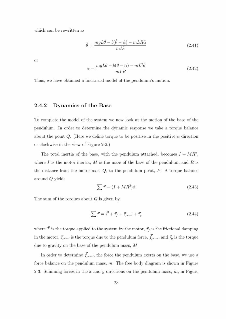
which can be rewritten as
θ =mgLθ − b(θ − α)−mLRα
mL2(2.41)
or
α =mgLθ − b(θ − α)−mL2θ
mLR(2.42)
Thus, we have obtained a linearized model of the pendulum’s motion.
2.4.2 Dynamics of the Base
To complete the model of the system we now look at the motion of the base of the
pendulum. In order to determine the dynamic response we take a torque balance
about the point Q. (Here we define torque to be positive in the positive α direction
or clockwise in the view of Figure 2-2.)
The total inertia of the base, with the pendulum attached, becomes I + MR2,
where I is the motor inertia, M is the mass of the base of the pendulum, and R is
the distance from the motor axis, Q, to the pendulum pivot, P . A torque balance
around Q yields∑
~τ = (I + MR2)α (2.43)
The sum of the torques about Q is given by
∑~τ = ~T + ~τf + ~τpend + ~τg (2.44)
where ~T is the torque applied to the system by the motor, ~τf is the frictional damping
in the motor, ~τpend is the torque due to the pendulum force, ~fpend, and ~τg is the torque
due to gravity on the base of the pendulum mass, M .
In order to determine ~fpend, the force the pendulum exerts on the base, we use a
force balance on the pendulum mass, m. The free body diagram is shown in Figure
2-3. Summing forces in the x and y directions on the pendulum mass, m, in Figure
23
m
fpend
-mg
M
P
Q
R T
-fpend
(b) (a)
g
Y
X
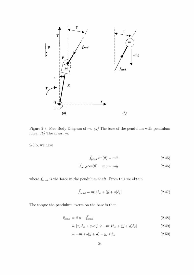
Figure 2-3: Free Body Diagram of m. (a) The base of the pendulum with pendulumforce. (b) The mass, m.
2-3.b, we have
~fpend sin(θ) = mx (2.45)
~fpend cos(θ)−mg = my (2.46)
where ~fpend is the force in the pendulum shaft. From this we obtain
~fpend = m[xex + (y + g)ey] (2.47)
The torque the pendulum exerts on the base is then
~τpend = ~q ×−~fpend (2.48)
= [xP ex + yP ey]×−m[xex + (y + g)ey] (2.49)
= −m[xP (y + g)− yP x]ez (2.50)
24

Substituting the appropriate equations of motion from Section 2.3, applying the
trigonometric identities used previously, and linearizing, we obtain
~τpend = m[R2α + RLθ − gRα]ez (2.51)
Gravity acting on the base of the pendulum produces a force, ~Fg = −Mgey, the
resulting torque on the motor is
~τg = ~q × ~Fg (2.52)
= [xP ex + yP ey]× [−Mgey] (2.53)
= −MgxP ez (2.54)
After substitution from equation (2.5),
~τg = −RMg sin(α)ez (2.55)
Note that since we have defined positive torque to be opposite of ez it will be necessary
to invert ~τg and ~τpend for use in equation (2.44).
The frictional damping torque, ~τf , can be determined by inspection and is made
positive in the direction of positive α
~τf = −cα (2.56)
Correcting the signs of each term to make torque positive in the direction of
positive α and substituting (2.51), (2.55) and (2.56) into equation (2.44) we obtain
the second equation of motion. The linearized result is
[(M + m)R2 + I]α = T − cα−mLRθ + (M + m)gRα (2.57)
25
2.5 Dynamics for Combined Pendulum and Cart
System
The dynamics of the combined system can found using equations (2.41) and (2.42) to
alternately eliminate θ and α from equation (2.57). From this we obtain the following
expressions:
α =T + MgRα− cα−mgR(θ − α) + bR
L(θ − α)
MR2 + I(2.58)
and
θ =−TR + gIθ + cRα + g[(M + m)R2](θ − α)− b
mL[(M + m)R2 + I)(θ − α)
L(MR2 + I)(2.59)
2.5.1 Change of Coordinates to α and β
The measurable coordinates in the simplest implementation of this system are α and
β, where α is the angle of the base, and β is the angle of the pendulum with respect
to the base such that β = θ−α, as shown in Figure 2-2. Thus, since we will measure
β with a simple potentiometer, it is advantageous to rewrite the system in the α and
β coordinate system.
Substituting β = θ − α into equation (2.58), we have
α =T + MgRα− cα−mgRβ + bR
Lβ
MR2 + I(2.60)
Now adding and subtracting the term gIα from equation (2.59) and grouping the
θ − α term we have
θ =−TR + gIα + cRα + g[(M + m)R2 + I](θ − α)− b
mL[(M + m)R2 + I)(θ − α)
L(MR2 + I)(2.61)
26

Substituting β = θ − α this becomes
θ =−TR + gIα + cRα + g[(M + m)R2 + I]β − b
mL[(M + m)R2 + I)β
L(MR2 + I)(2.62)
Calculating β we have
β = θ − α
=−T (R + L) + g(I −MRL)α + c(R + L)α
L(MR2 + I)
+g[(M + m)R2 + I + mRL]β − b[ (M+m)R2+I
mL+ R]β
L(MR2 + I)(2.63)
2.6 Results in State Determined Form
This system can now be written in state-determined form
~x = A~x + Bu (2.64)
where the input u is simply the applied torque, T , and the state vector, ~x is given by
~xT =[α α β β
](2.65)
The A and B matrices are determined directly from equations (2.60) and (2.63)
A =
0 1 0 0
MgRMR2+I
−cMR2+I
−mgRMR2+I
bRL(MR2+I)
0 0 0 1
g(I−MRL)L(MR2+I)
c(R+L)L(MR2+I)
g[(M+m)R2+I+mLR]L(MR2+I)
−b[(M+m)R2+I
mL+R]
L(MR2+I)
(2.66)
BT =[0 1
MR2+I0 −(R+L)
L(MR2+I)
](2.67)
This solution lacks the simple elegance of the classic inverted pendulum on a cart
system given in Section 2.1. However, the basic form is the same, with the addition
27

of two terms dependent on α. The first term quantifies the contribution to α resulting
from gravity on the base of the pendulum (~τg ∝ MgRα). The dependence of β on
α, however, is purely an artifact of the change of coordinates performed in section
2.5.1. Regardless of these differences, the design approach by full state feedback is
essentially unchanged.
28

Chapter 3
MATLAB Model of the Inverted
Pendulum
In analyzing the inverted pendulum problem, heavy use was made of MATLAB to
model the system and examine the effects of various inputs and changes to the model.
The following details the full state feedback approach employed here and the Simulink
model used to analyze the system.
3.1 Theory of state feedback
The idea behind full state feedback is to make the feedback signal, u, dependent on
the state of the system: u = −K~x, as shown in Figure 3-1. Thus our state equation,
~x = A~x + Bu, becomes
~x = (A−BK)~x (3.1)
Since the characteristic polynomial of this system is
|sI−A + BK| = (s + p1)(s + p2) . . . (s + pn) (3.2)
it is possible to place the poles of the system (p1, . . . , pn) at a desired location with
an appropriate choice of K, provided that the system is completely state controllable
and that all the states are available for feedback. For more information on the theory
29

x' = Ax+Bu y = Cx+Du
Pendulum Model in State-Space
K
Matrix Gain
u State vetor, x
Figure 3-1: Basic State Feedback
of state feedback see Modern Control Engineering by Ogata [2].
Ackermann’s formula for pole placement was used to place the closed loop poles
at −2± 1.5i,−10, and −10, given the linearized A and B matrices from Section 2.6.
For details of this procedure see Appendix B.2.
3.2 Simulink Model
Figure 3-2 shows the Simulink model with the additional blocks required to plot the
response of the system. The input and output blocks shown in the figure and discussed
below are borrowed from the MATLAB file penddemo.m. The detailed system model
with sensor gains is given in Figure 3-5.
3.2.1 Input
Since the model has no natural disturbances, it was necessary to create input dis-
turbances to observe the system response. In Figure 3-2 there is an offset, αref ,
subtracted from α. Since full state feedback systems are regulator systems, meaning
that they regulate to the origin of state space, this offset allows us to observe the step
response of the system as follows.
In this system the origin of state space is α = α = β = β = 0, when the pendulum
is balanced vertically and stationary. The offset has the effect of shifting the origin
30

Beta dot
t
y
0
Reference
x' = Ax+Bu y = Cx+Du
Pendulum Model in State-Space
Mux
K
Matrix Gain
Demux
Animation
alpha
Alpha dot
alpha_ reference
Beta
xT
Figure 3-2: Simulink Model of Full State Feedback with the MATLAB’s pendulumanimation output and output to file.
of state space. We denote shifted coordinates with a ′ symbol.
α′ = α− αref (3.3)
and
β′ = θ − α′ (3.4)
= θ − (α− αref ) (3.5)
= (θ − α) + αref (3.6)
= β + αref (3.7)
Since the reference offset is a constant it has no effect on the derivatives of α and β.
Thus, the new origin of state space becomes
α− αref = α = β + αref = β = 0 (3.8)
The origin of state space now corresponds to α and β non-zero, but equal and opposite.
Fortunately, this condition also corresponds to a vertical pendulum (θ = 0). Thus,
the introduction of this offset simply has the effect of stabilizing the pendulum at non-
31

zero α. A square wave offset supplied to α by the function generator in the upper
left of Figure 3-2, thus allows observation of the step response of the pendulum.
3.2.2 Output
The output blocks in Figure 3-2 include MATLAB’s graphical pendulum animation
and output to the workspace stored in the vector y.
Figure 3-3 graphically shows the pendulum balanced at non-zero α. The output
shown here has been slightly modified from MATLAB’s animation program pendan.m
to show the pendulum with the rotary base. For the modified code see Appendix B.5.
Figure 3-3: Modified MATLAB Pendulum Animation with pendulum balanced up-right at non-zero α.
For a more detailed analysis, Figure 3-4 plots the data output from Simulink in
the vector y, illustrating the response of the pendulum to a square wave offset in α.
It is apparent at steady state in Figure 3-4, that β is equal and opposite to α,
indicating that the pendulum is standing upright. The lower half of the plot shows
that θ is in fact equal to zero in the steady state.
It is worth note that, with damping equal to zero, as in the plots here, the values
of the gain matrix, K, are all negative. This means that with the feedback equal
to −K~x the control system is actually implementing positive feedback on all of the
states. Although this may seem surprising, it is correct. Consider the classic inverted
32

0 10 20 30 40 50 60 70 80 90 100-15
-10
-5
0
5
10
15
Ang
le (
de
gre
es)
Response of the Pendulum
A lphaB eta
0 10 20 30 40 50 60 70 80 90 100-15
-10
-5
0
5
10
15
Time (sec)
Ang
le (
de
gre
es)
Theta
Figure 3-4: The modelled pendulum response to square wave reference input.
pendulum on a cart with the pendulum balanced at x > 0 and x = θ = θ = 0.
Positive feedback indicates the system will initially respond by moving the cart in
the +x direction. This will cause the pendulum to lean back towards the origin with
θ negative. Because the gains on the θ feedback are much higher than on x, this
will cause the pendulum to correct by moving back towards x = 0. Thus, positive
feedback actually gives the desired response.
Looking at Figure 3-4 you can see that the pendulum does respond to the step
input by initially making deviations in α worse, causing θ to tilt in the direction of
the desired equilibrium.
3.2.3 Detailed System Model
Having established the basic system and stability, the next step is to model the phys-
ical system. Figure 3-5 shows the model of the complete system, including the gains
33

of all the sensors and components discussed in Chapter 4. For simplicity the output is
not shown. The gain matrix Ksys in the figure was determined by appropriately fac-
toring out the system gains from the K matrix previously found using Ackermann’s
Formula. More detail on this adjustment is available in Appendix B.3.
Kb
bridge
Kbp
beta_pot
Terminator
Kt
TachKa
Servo Ampiflier
Kp
Potentiometer
x' = Ax+Bu y = Cx+Du
Pendulum Model in State-Space
Km
Motor Torque constant
K
Matrix Gain (K_sys)
Kd
DifferentiatorGain
Demux
du/dt
V I T
alpha dot
Beta
alphaVoltage for alpha
Figure 3-5: State Feedback with the system gains added to the model
This specific system was used to model the effects of noise on various inputs,
non-linearities in the motor and general robustness to various conditions.
34

Chapter 4
Apparatus
4.1 2.010 Lab Platform
The inverted pendulum analyzed here was built on the MIT 2.010 undergraduate
motor control lab platform. The 2.010 lab features an Aerotech 1135DC servo motor,
mounted with its axis of rotation parallel to the ground and an aluminum inertia
attached to the output shaft, as illustrated in Figure 4-1. The motor has a built-in
tachometer and a potentiometer attached. Thus, velocity and position feedback for
the motor were provided. An Aerotech 4020-LS linear power amplifier was used as a
voltage controlled current source to power the motor. The relevant physical constants
and gains for this system, given in Table 4.1, were determined by Adiel Smith and
Ziaieh Sobhani in 2001 [3].
Table 4.1: Gains for the 2.010 Lab setup
Servo Amplifier Gain, Ka 1.9368 A/VMotor Torque Constant, Km 0.1697 Nm/ALoad Inertia, J 9.94×10⁴ kg/m2
Coulomb Friction Coefficient, Kf 0.0306 kgm2/secTachometer Gain Constant, Kt 0.0286 V/(rad/sec)Potentiometer Gain Constant, Kp 0.2504 V/rad
35

4.2 Pendulum Constructed
The pendulum base was clamped to the motor inertia in the orientation shown in
Figure 4-1. The pendulum was rigidly attached to the 14” shaft passing through P .
To measure the pendulum angle, β, a Bourns 6639S-1-103 precision potentiometer
was attached to this shaft via a flexible coupling and supported from below.
Motor Inertia, J
R
P
L
Q Q’
M
m
Pendulum Angle Potentiometer
Y
Z
Figure 4-1: Side view of the inverted pendulum setup. The base of the pendulumwas mounted on the inertia of a 2.010 lab motor.
The dimensions of the pendulum constructed are given in Table 4.2. The total inertia,
I, includes the aluminum inertia, J , and the inertia of the clamp for mounting the
pendulum base.
Table 4.2: Dimensions of the Pendulum Constructed
Radius of the arcing base, R 0.0725 mDistance from base to cg of pendulum, L 0.0532 mMass of the base, M 0.05338 kgTotal inertia, I 0.001293 kgm2
Mass of pendulum, m 0.00636 kg
36

4.3 Circuitry Added
4.3.1 Motor Range Limiting and Shut-off
The physical design of this system requires that α be stabilized. If α were to exceed
≈ 90 from vertical, the pendulum could strike the work bench and harm the motor
or the pendulum. To prevent the possibility of this happening a safety circuit was
designed to limit the range of the motor. The details of this circuit are given in
Appendix A.1. It functions by grounding the output to the servo amplifier when α
exceeds a specified range.
In addition to this feature, a toggle switch was provided as an emergency off switch
to ground the output to the servo amplifier.
4.3.2 Angle Measurement
Additional circuitry was necessary to measure the angle of the pendulum with respect
to the base, β, and to differentiate this signal to obtain the angular velocity of the
pendulum, β, required for full state feedback.
The β signal was obtained by placing the angle-measuring potentiometer in a
wheatstone bridge, the details of which are in Appendix A.3. The β signal was ob-
tained using an analog op-amp differentiation of the β signal. This circuit is discussed
in Appendix A.4.
Additional system gains introduced by these circuits are given in Table 4.3.
Table 4.3: Gains Introduced by Sensor Circuits
Gain of the β pot, Kbp 0.014529 V/
Gain of the bridge circuit, Kb 9.8147 V/VGain of differentiator, Kd 0.0105 V/V
37

4.3.3 Feedback
The feedback was accomplished by sending the four states (α, α, β, β) to a summing
op-amp with gains determined by specific test conditions in the MATLAB model. It
was convenient to use potentiometers on the feedback signals so that the gains could
be quickly adjusted for different test conditions.
38

Chapter 5
Procedure
5.1 Setup
The first step in testing this control system is mounting the pendulum assembly to
the motor inertia. It is critical that the pendulum be mounted such that the base of
pendulum is at the peak of the arc when α = 0. The position controller detailed in
Appendix A.2 was used to hold the motor inertia steady in the correct position while
mounting the pendulum.
After securing the pendulum we establish the β = 0 reference point. This was
done by first balancing the pendulum upright and securing the pot such that the β
signal was close to zero. The wheatstone bridge circuit discussed in Appendix A.3
was then adjusted to make β = 0 when the pendulum is balanced upright and α = 0.
Finally, one should check that the motor-range-limiting circuit is functioning cor-
rectly (shutting off the motor when α exceeds ≈ 45 from vertical) and that the signs
of all the feedback signals are positive in the positive direction of the motor.
5.2 Testing and Debugging
The procedure attempted for stabilizing the physical system was largely one of testing
and debugging. The MATLAB model was employed to determine the system gains
as discussed in Chapter 3, based on the specific conditions being tested. The four
39

feedback resistors in the summer op-amp were adjusted and primarily qualitative
observations were made of the system response. The most significant observation
made during debugging was that damping was not negligible.
It was immediately observed that viscous friction in the pendulum joint introduced
by the β pot assemblage was considerable. The pendulum was easy to stand upright,
so easy, in fact, that it was difficult to precisely determine where β = 0 really was.
Since the magnitude of the damping was not easy to measure, it was estimated by
observing the system response with different levels of damping added to the model.
By this method the value of b was estimated to be near 0.004 kgm2/sec.
Regarding the motor, it was determined previously by Smith and Sobhani [3] that
the primary friction was not viscous but coulomb in nature. This means that the
viscous friction, c, in the dynamic model was essentially zero, while the coulomb
friction in the motor was approximated as
Tf = −sign(α)Kf (5.1)
where the sign(α) term ensures that this effect always opposes the direction of motion
of the motor. Tf here represents the constant torque that is consumed by the friction
internal to the motor caused by gears and bearings. The Coulomb friction must be
overcome before any torque will register on the output shaft.1 This Coulomb friction
effect is commonly known as a dead zone or dead band. The magnitude of Kf , given
in Table 4.1, was found to be 0.0306 kgm2/sec2, which corresponds to Tf of 0.0306
Nm.
This dead band torque is larger than the peak torque of 0.0154 Nm required for
the stabilization of the pendulum modelled in Figure 3-4. This result explains the lack
of response observed in the physical system, since for moderate deviations the control
signal was overwhelmed by the dead zone of the motor. To counteract this effect
a circuit was designed to compensate for the dead zone by adding a corresponding
voltage to ”preload” the output signal to the motor. This circuit made it possible to
1The effects of stiction are not considered here.
40

observe the system response and enable further testing.
Following the initial compensation for the dead zone, it was observed that the
system response was asymmetric, consistently overcorrecting in the negative direction
and undercorrecting in the positive direction. This observation inspired a better
attempt at measuring the dead zone by observing the minimum voltage required
to make the motor turn. As expected, the values varied significantly depending
on direction and other effects, which probably include temperature, recent use, and
possibly even position of the motor.
It was difficult to measure the minimum voltage with accuracy or precision, how-
ever, the result was clearly asymmetric. The circuit discussed in Appendix A.5 was
implemented to better compensate for the asymmetric dead zone, based on the best
estimate of the size of the dead zone.
Unfortunately, even this better compensation failed to stabilize the system. Upon
examination of the effects of the dead zone in the MATLAB model (to be discussed in
Chapter 6), the attempt at stabilizing the inverted pendulum by the current method
in the time available was abandoned.
41

42
Chapter 6
Results and Discussion
The results of these tests were inconclusive. In theory the inverted pendulum with the
arcing base considered here is no more difficult to stabilize than the classic inverted
pendulum on a cart. However, the practical problems in implementing the control
system were considerable.
6.1 Damping
The effects of damping are believed to be the dominant cause of failure. Damping
in the pendulum joint, introduced primarily by the β potentiometer and the flexible
coupling joining it to the pendulum shaft, was significant. While this damping has
a large impact on the model, stabilization is possible, provided the damping is ac-
counted for. Damping in the pendulum joint hindered this investigation because the
magnitude of the damping was hard to measure or even estimate. A robust stabi-
lization would require eliminating this damping altogether or at least determining a
better way to measure it.
The effect of coulomb friction in the motor is a more serious problem because the
model has no way to compensate for this non-linearity. Examining the effect of the
motor dead zone in the MATLAB model showed that the system was intolerant to
even a small dead zone. In general, the simulated pendulum became oscillatory and
unstable as the magnitude of the dead zone increased. Figures 6-1 and 6-2 illustrate
43

this trend. The simulated responses shown here model the pendulum constructed with
an estimated damping of 0.004kgm2/sec. These plots show the pendulum regulating
to the origin, given an initial condition where it is balanced upright at α = 0.02 rad
(α ≈ 1).
0 1 2 3 4 5 6 7 8 9 10-1.5
-1
-0.5
0
0.5
1
1.5
Ang
le (
de
gre
es)
Response of the Pendulum with b=0.004kgm/sec, Tf=0
A lphaB eta
0 1 2 3 4 5 6 7 8 9 10-0.05
0
0.05
0.1
0.15
Time (sec)
Ang
le (
de
gre
es)
Theta
0 1 2 3 4 5 6 7 8 9 10-6
-4
-2
0
2
4
6
Ang
le (
de
gre
es)
Response of the Pendulum, b=0.004, Tf=0
A lphaB eta
0 1 2 3 4 5 6 7 8 9 10-0.2
0
0.2
0.4
0.6
0.8
Time (sec)
Ang
le (
de
gre
es)
Theta
Figure 6-1: The simulated pendulum response to an initial condition. With no deadzone the system is stable.
Figure 6-1 illustrates the stable response with no dead zone (Tf = 0). Figure 6-2,
however, illustrates how the system oscillates with increasing size of the dead zone. In
Figure 6-2.a, the pendulum oscillates between α ≈ ±2 with the dead zone modelled
as 1% of the measured dead zone on the 2.010 motor (Tf = 3.06×10⁻⁴). Figure 6-2.b
shows the oscillations increased to ≈ ±20 with a dead zone of 10% of the measured
value (Tf = 3.06× 10⁻³).
These oscillations quickly exceed the linear range of the model, indicating the
system is actually unstable for even a relatively small dead zone. The magnitude of
the oscillations was fairly independent of the initial condition given here; it increased
44

0 1 2 3 4 5 6 7 8 9 10-2
-1
0
1
2
An
gle
(d
eg
ree
s)
Response of the Pendulum with b=0.004kgm/sec, Tf=0.01*K
f
AlphaBeta
0 1 2 3 4 5 6 7 8 9 10-1
-0.5
0
0.5
1
Time (sec)
An
gle
(d
eg
ree
s)
Theta
(a)
0 1 2 3 4 5 6 7 8 9 10-20
-10
0
10
20
An
gle
(d
eg
ree
s)
Response of the Pendulum with b=0.004kgm/sec, Tf=0.1*K
f
AlphaBeta
0 1 2 3 4 5 6 7 8 9 10-10
-5
0
5
10
Time (sec)
An
gle
(d
eg
ree
s)
Theta
(b)
Figure 6-2: The pendulum oscillates with dead zone at (a) 1% and (b) 10% of esti-mated dead zone on the 2.010 motor.
45

moderately as the damping, b, increased and in general decreased as the pendulum
size increased. Since our experimental measurements of the dead zone threshold were
at best able to pinpoint the magnitude of the dead zone within 10%, stabilization of
the current system using preloading method of dead zone compensation was deemed
futile.
6.2 Recommendations
A general recommendation for future attempts at stabilization would be to make the
pendulum larger and sturdier. During testing it was observed that some backlash
developed in the mounting between the pendulum and the shaft to the β pot. While
larger issues limited the success of this study, a sturdier construction would easily
eliminate this problem and potential nonlinearities in the system. Due primarily to
safety concerns the pendulum constructed was very small. As a result the linear range
of motion for P was less than 7cm (≈ 3in). While the dimensions of the pendulum
have no impact on the ideal MATLAB model, the small pendulum made observation
and debugging of the system difficult. Furthermore, a bigger, more massive pendu-
lum would add robustness to unaccounted for damping. Since a larger plant would
naturally require larger torques while the dead zone remains constant, the effects of
the dead zone would be diminished.
Eliminating the dead zone altogether could be accomplished by one of two tech-
niques. Conceptually the most straightforward would be to add a torque feedback
loop around the motor. The result of the dead zone was that the output torque to the
system was less than that specified by the controller. Placing feedback around the
motor we could ensure the output torque matched the desired value. The difficulty
in this approach would be to measure the torque output of the motor. Provided this
torque could be measured, a torque feedback loop would be the simplest solution to
eliminating the dead zone.
A second solution to the dead zone problem would be to modify the system model
to control the position of the base rather than torque. From equation (2.40) the
46

transfer function for the pendulum only can be written as
Θ(s)
A(s)=
s(mLRs− b)
−mL2s2 − bs + mgL(6.1)
This system can be stabilized using root locus techniques, similar to those commonly
used with the classic linear inverted pendulum, as mentioned in section 2.1.2. Un-
fortunately, this approach involves considerable modifications to the control theory
presented here.
Unfortunately, issues with damping and the dead zone hindered the true goal of
this study, which was the stabilization of the inverted pendulum using simple analog
components. Obtaining the β signal via an op-amp differentiator was an anticipated
challenge for implementing full state feedback in this manner.
The analog differentiator employed here and discussed in detail in Appendix A.4
differed considerably from the theoretical response below frequencies of 1.5 Hz. Since
these low frequencies are important in this system it may be worthwhile to improve
the differentiator after the improvements listed above. This effect is not considered
as great because the model seemed to be robust to a factor of 2 miscalculation in Kd,
which should cover the difference for the relevant frequencies.
47

48

Appendix A
Circuits
A.1 Motor Range Limiting Circuit
The motivation behind this circuit was to limit the range of motion of the motor.
Since the motor is physically restricted to ≈ 180 of motion when the pendulum
assembly is mounted, it would be dangerous for the system to go unstable and have
the pendulum strike the work bench. The following circuit causes the motor to shut
off whenever the motor angle, α, exceeds a specified range—here ≈ 45 from vertical.1
1
2
2
A A
B B
+3
-2
V+
7
V-
4
6
U3
uA741
-1
F1
FPOLY
+3
-2
V+
7
V-
4
6
U1
uA741
Z1
IXGH40N60
Z2
IXGH40N60
10 10kR4
5kR5
5kR6
10kR7
10kR2
14kR3
12V
-12V
-12V
12V
12V
-
MicroSim Corporation20 FairbanksIrvine, CA 92718714-770-3022
Revision: January 1, 2000 Page of
Page Size: A
11
V_ref=~2V
V_out
NPN transistors
V_in proportional to alpha
Comparitors
Signal from control circuit
Signal to power amplifier
Relay
Figure A-1: This circuit limits the range of α to ±45.
49

Consider first the top half of the circuit in Figure A-1. The motor position, α,
was measured through a geared potentiometer with a gain of 0.2584 V/rad. Here this
signal was further amplified by a factor of 10, to obtain a working voltage range of
±4V, corresponding to the possible 180 of travel. The amplified input signal was
compared to an adjustable reference voltage of ≈ 2V, which corresponds to an α of
about 45 from vertical. When the amplified α input exceeds the reference voltage
on the 741 Operational Amplifier, (that is, when α exceeds the specified limit), the
output of the op amp will be high. This high output in turn activates an NPN
transistor through the resistor divider shown. When the NPN transistor is active,
current will flow through the relay, activating it and grounding the signal to the servo
amplifier. Providing this 0V input to the servo amplifier turns off the motor. Thus,
when α exceeds the set bound, the motor is turned off.
The lower half of this circuit performs the same operation on the inverted signal,
thus the motor has been effectively restricted to a range with absolute value of 45.
A.2 Motor Position Controller
It is critical for this system that the pendulum be mounted to the motor inertia such
that the pendulum pivot, P , is directly above Q (at the top of the arc) when α = 0.
The motor position controller, shown in Figure A-2, is used to hold the motor at
α = 0 so that the pendulum can be mounted correctly. This controller has a very
high gain and reacts quite forcefully when α is significantly different from zero. For
this reason, it is recommended to only engage the position controller after manually
aligning α to within ±15 of zero.
A.3 Pendulum Angle, β, Measurement
To measure the angular position of the pendulum a Bourns 6639S-1-103 precision
potentiometer was mounted on the shaft at the base of the pendulum with the flexible
coupling shown in Figure 4-1. This potentiometer has a resistance of 10KΩ linear
50

1
1
2
2
A A
B B
R59.8K
R2
22.1K
R3
9.79K
R1
100.4K
+3
-2
V+
7
V-
4
6
uA741
U1
+12V
-12V
-
MicroSim Corporation20 FairbanksIrvine, CA 92718714-770-3022
Revision: January 1, 2000 Page of
Page Size: A
11
V_alpha_dot
V_alpha*10
V_out
Figure A-2: The PD position controller used to hold the motor inertia at α = 0 whenmounting the pendulum.
within 1% through a range of 340. Since the MATLAB model indicated that the
system was sensitive to noise in the measurement of the pendulum angle, it was
decided to power the β pot with a 5V voltage regulator, which filters much of the noise
from the 12V power supply. With the regulator voltage of 4.94V, the potentiometer
gain for the β pot, Kbp, is
Kbp =4.94V
340= 0.01453V/ (A.1)
The β pot was wired as one side of a wheatstone bridge circuit, as shown in Figure
A-3. The primary reasons for choosing this circuit were the ability to obtain a positive
and negative signal from a single voltage regulator, the potential to filter out common
mode noise, and the convenience of being able to balance the circuit with a simple
adjustment of the balancing pot, R8. With the resistor values used in Figure A-3, this
circuit was able to adjust the zero position of β through a wide angle and alleviate
much concern about the orientation of the β pot during mounting.
After mounting the β pot and zeroing the wheatstone bridge, the output voltage
difference (Va − Vb) is directly proportional to β. In order to reference this voltage
51

1
1
2
2
A A
B B5.03K
R5
2.18KR6
3.8K
R7
POT
R1=10K
+3
-2
V+
7
V-
4
6
U1
uA741
98.1K
R11
10.0K
R1010.0K
R9
50K
R898.1K
R12
+5v
+12V
-12V
0V
V_out
-
MicroSim Corporation20 FairbanksIrvine, CA 92718714-770-3022
Revision: January 1, 2000 Page of
Page Size: A
11
Va
Vb
Pendulum Angle Sensor
Wheatstone Bridge Differential Op Amp
Balancing Pot
Figure A-3: The pendulum angle measurement was obtained by placing the poten-tiometer measuring β in a wheatstone bridge circuit and then using a differentialamplifier to amplify the signal and reference it to ground.
difference to ground for use in the rest of the control circuit, the voltage output of the
wheatstone bridge was passed through a differential amplifier, as shown in the right
in Figure A-3. With R9 = R10 = 10.0KΩ and R11 = R12 = 98.1KΩ, the differential
amplifier obeys the following relation
Vout =R11
R10
(Va − Vb) = 9.81(Va − Vb) (A.2)
where Vout is referenced to ground and the expected gain of the bridge circuit, Kb,
due to the differential amplifier, is 9.81. This prediction corresponds very well with
the measured gain of 9.8147, plotted in Figure A-4.
A.4 Differentiator Circuit for β
In keeping with the minimalist approach to this this stabilization problem, the an-
gular velocity of the pendulum, β, was obtained by differentiating the position signal
52

Differential Amplifier for Beta
y = 9.8147x + 0.0039
R2 = 1
-8
-6
-4
-2
0
2
4
6
8
-0.8 -0.6 -0.4 -0.2 0 0.2 0.4 0.6 0.8
V_a-V_b from Wheatstone Bridge (V)
V_o
ut
(V)
Figure A-4: The gain of the differential amplifier agreed well with the theory and wasvery linear.
obtained as in Section A.3. Figure A-5 shows the circuit designed to differentiate β.
1
1
2
2
A A
B B
R1
99.3K
C1
.105u
+3
-2
V+
7
V-
4
6
U1
741
R2
100.1K
C2
25.8nF
-12V
12V
-
MicroSim Corporation20 FairbanksIrvine, CA 92718714-770-3022
Revision: January 1, 2000 Page of
Page Size: A
11
V_in
V_out
Figure A-5: This circuit was used to differentiate the angular position, β, to obtainthe angular velocity, β.
The transfer function for this differentiator circuit is
Vout(s)
Vin(s)=
−R2C1s
(R1C1s + 1)(R2C2s + 1)(A.3)
where the break frequencies are designed at 1/R1C1 = 95.9rad/sec= 15.3Hz and
1/R2C2 = 352rad/sec= 56.0Hz. The upper break frequency was chosen to help
53

eliminate high frequency noise and the lower bound break frequency high enough to
capture our expected response.
Figure A-6 plots the theoretical bode plot for this transfer function using MAT-
LAB’s bode function as well as the experimental data collected for the actual circuit.
The resulting circuit differentiates well up to 15Hz, although the gain does not follow
the theory exactly below approximately 2Hz.Bode Diagrams
-40
-35
-30
-25
-20
-15
-10
-5
0Measured and Predicted Differentiator Response
Am
plitu
de (
dB)
Theory Experimental Data
100 101 102 103 104-300
-250
-200
-150
-100
-50
Frequency (rad/sec)
Pha
se (
degr
ees)
Figure A-6: The differentiator circuit performs close to the theory at higher frequen-cies but not so well at low frequencies.
A.5 Dead Zone Compensation Circuit
Testing demonstrated that the dead zone overwhelmed the control signal. Since the
control system has no way of compensating for this non-linearity in the motor, a
separate circuit was designed to try to compensate for the dead zone of the motor.
The dead zone was measured by slowly increasing the voltage into the servo am-
54

plifier and observing the minimum voltage required to make the motor turn. This
voltage was found to be approximately −0.08V in the −α direction and 0.12V in
the +α direction. These values correspond to torques of −0.027Nm and 0.040Nm,
respectively, which seems reasonable given that in Smith and Sobhani found the value
of the coulomb friction torque, Tf , to be 0.031Nm [3]. The asymmetry found here was
also present in other motors tested and accounted well for the observed asymmetric
behavior of the system.
The simple compensation scheme employed here is to ”preload” the output signal.
Essentially, we desire a circuit to perform the following math operation, which, if the
compensating voltages were known exactly, should effectively remove the dead zone:
Vout =
Vin + 0.12V if Vin > 0
Vin − 0.08V if Vin < 0
Figure A-7 shows the circuit used to compensate for this asymmetric dead zone.
Because, the voltage offset effect of the dead zone is fairly small, the circuit actually
operates on the desired voltage amplified by a factor of ten, adding an offset voltage
of 1.2V or −0.8V as appropriate and then reducing the signal by a factor of ten to
obtain the desired output1. The first two op-amps in Figure A-7 serve as a simple
comparator and inversion, which determine the sign of the input signal, causing Vs
to be high (≈ 10.5V) when Vin is positive and low (≈ −10.5V) when Vin is negative.
The interesting part of this circuit is the voltage divider input to the third op-
amp. This divider is designed such that when Vs is high the offset voltage, Voff is
1.20V and when Vs is low Voff is −0.80V. The resistor values given to achieve this
are approximate. In the physical implementation a 10K potentiometer was used in
place of R4 and R5. This pot was adjusted such that, without Vs connected, Voff
was midway between the positive and negative offset voltages, here 0.2V. A 50K pot
was then used in place of resistor R3 and adjusted such that the desired positive
1This amplification and deamplification could be a problem if we reach the saturation limits ofthe op amps. In this case, if our desired output signal exceeds ≈ 1V, this amplification would havesaturated the op amp, resulting in some loss of the signal. Fortunately, our control signals were lowenough that this did not become a problem.
55

1
1
2
2
A A
B B+3
-2
V+
7
V-
4
6
U2
uA741
+3
-2
V+
7
V-
4
6
U1
uA741
5k R4
4.8k
R5R3
26k
100k
R6
10k
R8
+3
-2
V+
7
V-
4
6
U3
uA74110k
R1
10k
R2
100k
R7
+12V
-12V
+12V
-12V
+12V
-12V
+12V
-12V
-
MicroSim Corporation20 FairbanksIrvine, CA 92718714-770-3022
Revision: January 1, 2000 Page of
Page Size: A
1 1
V_s
V_in
V_outV_off
ComparitorUnity Gain Inversion
Summer Gain=0.1
Asymmetric Resistor Divider
Figure A-7: This circuit was designed to compensate for the asymmetric dead zoneof the motor.
and negative offset voltages were correct. This calibration was necessary because the
voltage rails and the saturation output of the op amps vary with the power supply
and op amps used, making a precise calculation of the resistor values tedious and
unnecessary.
The last op amp simply sums the offset voltage to the original signal and then
divides by ten to compensate for the earlier amplification by ten. The result of
implementing this circuit was to improve symmetry in the response, but still the
system was far from stable.
56

Appendix B
MATLAB Code
Below is given the MATLAB code used in the simulations of the pendulum. The
file thesis_init.m initializes all the necessary constants as well as the state space
matrices A,B,C and D. The file poleplacement.m uses Ackermann’s formula to
obtain the state feedback gain matrix, K. Finally the file Kz_system, modifies K to
account for the system gains due to sensors and hardware in the system considered.
The full simulink model used, ziapenddemo.mdl, is shown here in Figure B-1. The
modifications to MATLAB’s pendulum animation pendan.m is given, as well as the
file plot_penddemo.m, which was used to plot the output response of the pendulum.
B.1 Initialization
%thesis_init.m
%This file initialized the values of all constants in the system.
global A B step num
L=.0532; %m
m=.0636; %kg
R=.0725; %m, base of pendulum from motor axis
g=9.81; %m/sec^2
b=0.004; %hinge damping, adjusted for testing
c=0; %Friction in the motor was determined to be coulomb only
57

% so viscous coefficient is zero
%%%%%%%Begin Dynamics for Rotary Base%%%%%
%Calculate the total inertia:
M=.05338; %Mass of the pendulum base bracket
R_clamp=.0375; %m
M_clamp=.2106; %Mass of the clamp (kg)
J=9.97e-4; %kg*m^2 inertia of the motor
I=J+M_clamp*R_clamp^2; %kgm^2, total inertia
%Input A and B matrices for pendulum with arcing base
den=M*R^2+I; %The common denominator of all terms
A_arc=[0 1 0 0; M*g*R/den -c/den -m*g*R/den b*R/(L*den); 0 0 0 1;
g*(I-M*R*L)/(L*den) c*(R+L)/(L*den) g*((M+m)*R^2+I+m*L*R)/(L*den)
-b*(((M+m)*R^2+I)/(m*L)+R)/(L*den)]
B_arc=[0; 1/den; 0; -(R+L)/(L*den)]
%% Initialize the A, B, C and D matrices for Simulink and poleplacement
A=A_arc;
B=B_arc;
C_all=eye(4); %Full state feedback
D=zeros(4,1);
%Simulink Constants:
Ka=1.9368; %Amplifier Gain A/V
Km=.1697; %Nm/A
Kf=.0306; %kg*m^2/sec^2, Coulomb friction coefficient
Kt=.0286; %V/(rad/sec)
Kp=.2504; %V/rad
Kbp=.014529; %calculated theoretical v/degree of beta pot
Kbp=Kbp*180/pi; %V/rad
Kd=0.0105; %R2C1
Kb=9.8147; %Gain differential amplifier after wheatstone bridge
Tzf=0; %initialize dead zone to zero
step=0.0022; %initialize step input magnitude for signal generator
num=1000; %length of the output vector
58

B.2 Poleplacement
%poleplacement.m
%
%This file uses Ackermann’s Formula to determine the K matrix.
%It also calls thesis_init and Kz_system, so running poleplacement.m
%sets up everything necessary to run the simulink file ziapenddemo.mdl
global A B
thesis_init;
M=[B A*B A*A*B A*A*A*B];
rank(M) %Rank of the M matrix needs to be 4 for this
%system to be fully state controllable
%ans =
%
% 4
% Establish the Desired Characteristic Equation/closed loop poles
J=[-2+1.5*i 0 0 0;0 -2-1.5*i 0 0; 0 0 -10 0; 0 0 0 -10]
% Use Ackermann’s Formula to find the Feedback matrix K, that
% will yield the desired closed loop poles and print K’ to screen:
phi=polyvalm(poly(J), A);
K=[0 0 0 1]*inv(M)*phi;
K_transpose=K’
%Run the file Kz_system, which factors out the system gains and then
%print to screen the gains to be implemented in K_summer
Kz_system;
systemgain=Kz_sys’
B.3 Calculate System Gains
The following code modified the K matrix found using Ackermann’s Formula to com-
pensate for the system gains. For example, all of the control signals pass through the
servo amplifier and the motor, thus, in the first step, the entire gain matrix is divided
by Ka and Km. This process is continued for each individual control signal to obtain
59

the system gain matrix, Ksys.
%Kz_system
%
%Determine the system gain constant Kz_sys from the poleplacement result for K
Kz_sys=K/Km/Ka; %These are the gains common to all inputs
%Gain adjustments for specific signals
Kz_sys(1)=Kz_sys(1)/Kp; %alpha
Kz_sys(2)=Kz_sys(2)/Kt; %alpha_dot
Kz_sys(3)=Kz_sys(3)/Kbp/Kb; %beta
Kz_sys(4)=Kz_sys(4)/Kbp/Kb/Kd; %beta_dot
B.4 Full Simulink Model
The full Simulink model used is shown in Figure B-1. The input and output blocks
including the graphical animation came from MATLAB’s Simulink example file on
the inverted pendulum, penddemo.mdl, which can found by typing penddemo at the
MATLAB prompt. The graphical output for the pendulum response was invaluable
for quick observations of the system stability. The detailed pendulum response was
plotted by outputting the system states to the workspace. These states were stored
in the vector, y, while the time was stored in t.
B.5 Pendulum Animation
MATLAB’s pendulum animiation was modifed to make the output image reflect the
inverted pendulum with a rotary base. In the file pendan.m the following changes
were made to the function LocalPendSets:
function LocalPendSets(time,ud,u)
%%%%%%%Modified Code%%%%%%
%u(2) ALPHA
%u(3) BETA
60

Ktp
theta_pot
Kd
diff gain
Kb
bridge
1/Kp*20
alpha ref gain
t
y
Terminator
Kt
TachKa
Servo Ampiflier
0
Reference Kp
Potentiometer
x' = Ax+Bu y = Cx+Du
Pendulum Model in State-Space
Mux
Km
Motor Torque constant
MotorDead Zone
K
Matrix Gain (Kz_sys)
du/dt
Derivative
Demux
? ? ?
Coulomb &Viscous Friction
Animation
V I T
alpha dot
u
Voltage for alphaalpha
Beta
X_ reference
Figure B-1: The Full Simulink Pendulum Model.
%THETA=u(2)+u(3)
XDelta = 0.2; %width of the base block
PDelta = 0.2; %width of the pendulum
R = 3;
L = 4;
arrowwidth = 2;
XBaseTop = R*sin(u(2));
YBaseTop = R*cos(u(2));
PDcosA = XDelta*cos(u(2));
PDsinA = -XDelta*sin(u(2));
XPendTop = L*sin(u(3)+u(2))+XBaseTop;
YPendTop = L*cos(u(3)+u(2))+YBaseTop;
PDcosT = PDelta*cos(u(3));
PDsinT = -PDelta*sin(u(3));
set(ud.Cart,...
’XData’, [XBaseTop-PDcosA XBaseTop+PDcosA; -PDcosA PDcosA],...
’YData’, [YBaseTop-PDsinA YBaseTop+PDsinA; -PDsinA PDsinA]);
set(ud.Pend,...
’XData’,[XPendTop-PDcosT XPendTop+PDcosT;...
XBaseTop-PDcosT XBaseTop+PDcosT], ...
’YData’,[YPendTop-PDsinT+YBaseTop YPendTop+PDsinT+YBaseTop;...
-PDsinT+YBaseTop PDsinT+YBaseTop]);
set(ud.TimeField,...
’String’,num2str(time));
set(ud.RefMark,...
’XData’,u(1)+[-arrowwidth 0 arrowwidth]);
61

%%%%%%%Modified Code%%%%%%%%
%%%%Original Code%%%%%%%
%XDelta = 2; %width of the base block
%PDelta = 0.2; %width of the pendulum
%XPendTop = u(2) + 12*sin(u(3));
%YPendTop = 12*cos(u(3));
%PDcosT = PDelta*cos(u(3));
%PDsinT = -PDelta*sin(u(3));
%set(ud.Cart,...
% ’XData’,ones(2,1)*[u(2)-XDelta u(2)+XDelta]);
%set(ud.Pend,...
% ’XData’,[XPendTop-PDcosT XPendTop+PDcosT; u(2)-PDcosT u(2)+PDcosT], ...
% ’YData’,[YPendTop-PDsinT YPendTop+PDsinT; -PDsinT PDsinT]);
%set(ud.TimeField,...
% ’String’,num2str(time));
%set(ud.RefMark,...
% ’XData’,u(1)+[-XDelta 0 XDelta]);
%%%%%Original Code%%%%%%
% Force plot to be drawn
pause(0) drawnow
% end LocalPendSets
B.6 Plotting Output
The following code plotted the data collected in the output vector y during simula-
tions.
%plot_penddemo.m
%
%plot ziapenddemo response
close all;
hold on;
subplot(2,1,1),
plot(t, y(:,2)*180/pi, ’b:’,t, y(:,3)*180/pi, ’b-’)
ylabel(’Angle (degrees)’);
title(’Response of the Pendulum’);
62

legend(’Alpha’,’Beta’)
subplot(2,1,2),plot(t, (y(:,2)+y(:,3))*180/pi,’b-’);
xlabel(’Time (sec)’);
ylabel( ’Angle (degrees)’);
legend(’Theta’);
63

64

Bibliography
[1] Horowitz, Paul and Winfield Hill. The Art of Electronics. 2nd ed. Cambridge,
Eng.: Cambridge University Press, 2001.
[2] Ogata, Katsuhiko. Modern Control Engineering. 3rd ed. Upper Saddle River, NJ:
Prentice-Hall, 1997.
[3] Smith, Adiel and Ziaieh Sobhani. Data collected in MIT’s 2.010 Lab. Spring,
2001.
65