Embed Size (px)
Citation preview
Zhuan, Xin (2018) Growth and remodelling of the left ventricle post
myocardial infarction. PhD thesis.
https://theses.gla.ac.uk/30738/
Copyright and moral rights for this work are retained by the author
A copy can be downloaded for personal non-commercial research or study,
without prior permission or charge
This work cannot be reproduced or quoted extensively from without first
obtaining permission in writing from the author
The content must not be changed in any way or sold commercially in any
format or medium without the formal permission of the author
When referring to this work, full bibliographic details including the author,
title, awarding institution and date of the thesis must be given
Enlighten: Theses
https://theses.gla.ac.uk/
Growth and remodelling of the left ventricle post
myocardial infarction
August 2018

Declaration of AuthorshipI, XIN ZHUAN, declare that this thesis titled, ‘Growth and Remodelling of the Left Ventricle
Post Myocardial Infarction’ and the work presented in it are my own. I confirm that:
This work was done wholly or mainly while in candidature for a research degree at this
University.
Where any part of this thesis has previously been submitted for a degree or any other
qualification at this University or any other institution, this has been clearly stated.
Where I have consulted the published work of others, this is always clearly attributed.
Where I have quoted from the work of others, the source is always given. With the excep-
tion of such quotations, this thesis is entirely my own work.
I have acknowledged all main sources of help.
Where the thesis is based on work done by myself jointly with others, I have made clear
exactly what was done by others and what I have contributed myself.
Signed:
Date:
i

“If living in a world using Maths as language, I want to be a rock star.”
AbstractLiving organs in human bodies continuously interact with the in vivo bio-environment, while
reshaping and rearranging their constituents, responding to external or internal stimuli through
life cycles. For instance, living tissues adjust the growth (or turnover) rates of their constituents
to develop (volumetric and mass) changes as the tissues adapt to the pathological or physi-
ological changes in bio-environment. From the perspective of biomechanics, changes in the
bio-environment will induce the growth and remodelling (G&R) process and reset the mechan-
ical environment. Consequently, the mechanical cues will feed back to G&R processes. In the
long run, the interaction between G&R and the mechanical response of living organs plays an
important role in regulating the organ formulation or pathological growth.
To understand the interaction between the mechanical response and the G&R process, an im-
portant ingredient in evaluating the involved mechanics is knowledge of the solid mechanical
properties of the soft tissues. Residual stress, resulting from G&R of soft tissues, is important in
modelling the mechanics of soft tissues, which still presents a modelling challenge for includ-
ing residual stress in cardiovascular applications. For G&R of living organs, changes of tissue
structure and volume are also important determinants for organ development. This raises aca-
demic challenges for the understanding of the evolution of material properties and mechanical
response of living tissues within a dynamic environment.
To investigate the stress states (residual strain or residual stress) of living organs, the experi-
mental results showed that the arterial slices would spring open after cutting along the radial
directions, which indicates the residual strain in organs estimated by the opening angle [23].
The residual strain, which is the elastic strain between zero-stress and no-load states, indicates
the existence of residual stress after removal of the external loads. The residual stress is consid-
ered to modulate the growth and remodelling process in living organs. The evolution of residual
stress could relieve the information about the history of growth, which could help to better the
understanding of the formation of organs and the development of diseases.
Besides the residual stress, G&R processes are regulated by other factors, while the principles
governing those mechanism are still not fully understood. Obviously, improving knowledge in
this particular field will give huge potential for the design and optimization of clinical treatments
to efficiently save more lives.
From a general mechanics perspective to investigate the G&R process in living tissues, the ques-
tions are: How does the residual stress influence the fibre remodelling and the material properties
of entire organs? How to determine the combined effects of growth (in the stressed configura-
tion) and remodelling on the fibre structure? How to develop a framework for investigating
G&R processes occurring in the stressed configuration?
For arteries, multiple layer models are developed to analytically study residual stress in living
organs. For the heart, due to its complex structure and geometry, most previous studies used the
unloaded configuration or one-cut configuration as the stress-free configuration to estimate the
stress state. However, both experimental and theoretical studies have suggested that: 1) residual
stress will significantly influence the stress distribution in the heart. 2) a simple (or single)
cut does not release all the residual stress in the heart. We build a multi-cut model and show
that multiple cuts are required to release the residual stresses in the left ventricle. Our results
show that with the 2-cut and 4-cut models (one radial cut followed by circumferential cuts),
agreement with the measured opening angles and radii can be greatly improved. This suggests
that a multi-cut model should be used to predict the residual stresses in the left ventricle, at least
in the middle wall region. We further show that tissue heterogeneity plays a significant role in
the model results, and that an inhomogeneous model with combined radial and circumferential
cuts should be used to estimate the correct order of magnitude of the residual stress in the heart.
Understanding the healing and remodelling processes induced by myocardial infarction (MI)
of the heart is important and the mechanical properties of the myocardium post-MI can be in-
dicative for effective treatments aimed at avoiding eventual heart failure. MI remodelling is a
multiscale feedback process between the mechanical loading and cellular adaptation. In this
thesis, we use an agent-based model to describe collagen remodelling by fibroblasts regulated
by chemical and mechanical cues after acute MI, and upscale into a finite element (FE) 3D left
ventricular model. This enables us to study the scar healing (collagen deposition, degradation
and reorientation) of a rat heart post-MI. Our results, in terms of collagen accumulation and
alignment, compare well to published experimental data. In addition, we show that different
shapes of the MI region can affect the collagen remodelling, and in particular, the mechanical
cue plays an important role in the healing process.
For volumetric growth, recently, when the idea of growth is applied to study the evolution of
organ formations, it’s usually assumed that growth always occurs in the natural (reference) con-
figuration. In some researches, it is assumed that the growth could release all the residual stress,
and that further growth will start from the updated but stress-free configuration. However, liv-
ing organs are actually exposed to external loading all the time, while the growth should occur
from the residually-stressed current configuration. In this thesis, A theoretical framework is de-
veloped to calculate the mechanical behaviour of soft tissue after introducing inhomogeneous
growth in a residually-stressed current configuration, which avoids assuming that the growth oc-
curs in a ‘virtual’ reference configuration. Moreover, the theoretical framework is introduced to
couple the growth and fibre remodelling process to describe the mechanical behaviour of living
tissues.
AcknowledgementsIt’s my great honor to express my sincere gratitude to all the people and organizations who offer
helps and supports during my PhD period.
I would like to thank my supervisors Prof. Raymond Ogden and Prof. Xiaoyu Luo. They both
shared their solid academic fundamentals and wide views on researching with my during my
research. Prof. Ogden is one of the greatest scientists I ever met. During period to develop my
own research interests, his effects are the sources of enthusiasm and inspirations to go through
the hardness. Considerately, He gives me keys to open the doors to the hidden academic world.
Prof. Luo shares her great experience during my research program, which I deeply appreciated.
She can always sense my mistakes by simply checking my calculation results, rather than going
through all details. She is considered as a ‘research magic’ charming me. I somehow self-
centered during my research, especially when I tried to develop the methodology or theoretical
frameworks. They both are inspiriting and patient to guide me to the proper directions, making
me continuously improve myself to explore the academic world.
The School of Mathematical and Statistic provided a joyful environment to conduct my re-
search. I met the fantastic researchers here, and also had opportunities to experience the greatest
education system in the world. Many thanks for University of Glasgow shelling my during my
second longest student period, which is taken as my home ever of my life. I appropriated ev-
eryone sharing his/her knowledge and experience with me here, especially my colleges from
research group.
My families offer their unconditional loves and effects to support and heal me from all emotional
or physical hardnesses. Without them, I can’t be no where. It’s my best lucky to have them as
my parents, well-being wife, grandpa and all other relatives.
I would like to thank my country and people. I’m proud to be one of Chinese people, whose
home country has a long history but going through so many misfortunes. We are the witnesses
for a upcoming great historic era of China which applies its energetic motivations to contribute
to the rest of world. It’s my fortune to live in this time.
It’s my great pleasure to feedback my knowledge and creativities to the social and academic
communities in my rest life.
v
Contents
Declaration of Authorship i
Abstract iii
Acknowledgements v
List of Figures x
List of Tables xv
Abbreviations xvi
Symbols xvii
1 Introduction 11.1 Residual Stress and Opening-cut Method . . . . . . . . . . . . . . . . . . . . . 21.2 Coupled Agent-based and Elastic Modelling of Remodelling of Left Ventricle
Post-myocardial Infarction . . . . . . . . . . . . . . . . . . . . . . . . . . . . 31.3 Volumetric Growth from a Residually-stressed (Current) Configuration . . . . . 51.4 Research Aims . . . . . . . . . . . . . . . . . . . . . . . . . . . . . . . . . . 71.5 Outline of Thesis . . . . . . . . . . . . . . . . . . . . . . . . . . . . . . . . . 7
2 Basic Nonlinear Elastic Deformation Theory 92.1 Deformation and Strain . . . . . . . . . . . . . . . . . . . . . . . . . . . . . . 9
2.1.1 Observers and Frame of Reference . . . . . . . . . . . . . . . . . . . . 92.1.2 Configuration and Deformation Gradient . . . . . . . . . . . . . . . . 112.1.3 Cumulative Deformation and Polar Decomposition of Deformation Tensor 13
2.1.3.1 Cumulative Deformation . . . . . . . . . . . . . . . . . . . 132.1.3.2 Polar Decomposition of Deformation Tensor . . . . . . . . . 14
2.1.4 Deformation of Volume and Surface . . . . . . . . . . . . . . . . . . . 152.1.5 Strains and Stretch . . . . . . . . . . . . . . . . . . . . . . . . . . . . 15
2.2 Stress and Balance Laws . . . . . . . . . . . . . . . . . . . . . . . . . . . . . 162.2.1 Conservation of Mass . . . . . . . . . . . . . . . . . . . . . . . . . . 162.2.2 Momentum Balance Equation . . . . . . . . . . . . . . . . . . . . . . 172.2.3 Stress Tensors and Motions . . . . . . . . . . . . . . . . . . . . . . . 18
2.2.3.1 Cauchy Stress Tensor . . . . . . . . . . . . . . . . . . . . . 182.2.3.2 Nominal Stress and Lagrangean Balance Equation . . . . . . 19
vi
Contents vii
2.3 Constitutive Laws and Strain-energy Functions . . . . . . . . . . . . . . . . . 192.3.1 Constitutive Laws . . . . . . . . . . . . . . . . . . . . . . . . . . . . 192.3.2 Strain-energy Function . . . . . . . . . . . . . . . . . . . . . . . . . . 20
2.3.2.1 Deformation Constraints . . . . . . . . . . . . . . . . . . . 232.3.2.2 Strain Energy Function with Invariants . . . . . . . . . . . . 242.3.2.3 SEF for Mixture Materials . . . . . . . . . . . . . . . . . . . 252.3.2.4 The SEF for a Fibre-reinforced Material . . . . . . . . . . . 26
2.4 Summary . . . . . . . . . . . . . . . . . . . . . . . . . . . . . . . . . . . . . 30
3 Literature Review: Theories of Residual Stress in Living Organs Estimated by theOpening-angle Method 323.1 Residual Stress Estimated by an One-cut Model . . . . . . . . . . . . . . . . . 333.2 Residual Stress Estimated by a Multiple-cut Model . . . . . . . . . . . . . . . 38
3.2.1 Multiple-layer Model Using the Volumetric Growth Approach . . . . . 383.2.2 Multiple Layer Model with Mass Growth Approach . . . . . . . . . . 43
3.3 Summary . . . . . . . . . . . . . . . . . . . . . . . . . . . . . . . . . . . . . 43
4 Literature Review: Theories of Growth and Remodelling for Living Tissues 444.1 Remodelling of (Collagen) Fibre-reinforced Soft Tissues . . . . . . . . . . . . 45
4.1.1 G&R Process for Fibre-reinforced Tissues (from Cell Level to TissueLevel) . . . . . . . . . . . . . . . . . . . . . . . . . . . . . . . . . . . 47
4.2 Volumetric Growth of Soft Tissues . . . . . . . . . . . . . . . . . . . . . . . . 504.2.1 Volumetric Growth with Kinematic Approach . . . . . . . . . . . . . . 504.2.2 Mass Growth . . . . . . . . . . . . . . . . . . . . . . . . . . . . . . . 57
4.3 Summary and Theoretical Gaps . . . . . . . . . . . . . . . . . . . . . . . . . . 62
5 Residual Stress from Multi-cut Opening Angle Models of the Left Ventricle 645.1 Introduction . . . . . . . . . . . . . . . . . . . . . . . . . . . . . . . . . . . . 645.2 Methodology . . . . . . . . . . . . . . . . . . . . . . . . . . . . . . . . . . . 65
5.2.1 1-Cut Model . . . . . . . . . . . . . . . . . . . . . . . . . . . . . . . 675.2.2 2-Cut Model . . . . . . . . . . . . . . . . . . . . . . . . . . . . . . . 695.2.3 4-Cut Model . . . . . . . . . . . . . . . . . . . . . . . . . . . . . . . 73
5.3 Results . . . . . . . . . . . . . . . . . . . . . . . . . . . . . . . . . . . . . . . 755.3.1 Modelling Parameters . . . . . . . . . . . . . . . . . . . . . . . . . . 755.3.2 Results for the Homogeneous Myocardium Model . . . . . . . . . . . 775.3.3 Results for the Heterogeneous Myocardium Model . . . . . . . . . . . 78
5.4 Discussion . . . . . . . . . . . . . . . . . . . . . . . . . . . . . . . . . . . . . 785.4.1 Effect of Shear Stress . . . . . . . . . . . . . . . . . . . . . . . . . . . 81
5.4.1.1 Results to Compare the Solutions for Tissues with One andSymmetric Fibre Families . . . . . . . . . . . . . . . . . . . 85
5.4.2 Deformation Continuity and Stress Continuity . . . . . . . . . . . . . 875.4.3 Subsequent Elastic Deformation after Radial Cut on 1 cut Configuration 88
5.5 Conclusion . . . . . . . . . . . . . . . . . . . . . . . . . . . . . . . . . . . . 92
6 A Coupled Agent-based and Hyperelastic Modelling of the Left Ventricle Post My-ocardial Infarction 946.1 Introduction . . . . . . . . . . . . . . . . . . . . . . . . . . . . . . . . . . . . 946.2 Methodology . . . . . . . . . . . . . . . . . . . . . . . . . . . . . . . . . . . 96
6.2.1 Geometry of LV Model . . . . . . . . . . . . . . . . . . . . . . . . . . 966.2.2 Agent-based Model . . . . . . . . . . . . . . . . . . . . . . . . . . . . 97
6.2.2.1 Chemokine Concentration . . . . . . . . . . . . . . . . . . . 97
Contents viii
6.2.2.2 Fibroblast Migrations Regulated by Environmental Cues . . 986.2.2.3 Remodeling of the Collagen Fibre Structure . . . . . . . . . 1006.2.2.4 Upscaling the Fibre Structure from the Fibre Level to the Tis-
sue Level . . . . . . . . . . . . . . . . . . . . . . . . . . . . 1016.2.3 Constitutive Laws for Myocardium . . . . . . . . . . . . . . . . . . . 102
6.2.3.1 Modified HO Model with Fibre Orientation Density Function 1026.2.3.2 Exclusion of the Compressed Fibres . . . . . . . . . . . . . 1036.2.3.3 Change of Basis from Cartesian to Local Coordinates . . . . 104
6.2.4 Coupled Agent-based and FE Model . . . . . . . . . . . . . . . . . . . 1056.3 Results . . . . . . . . . . . . . . . . . . . . . . . . . . . . . . . . . . . . . . . 106
6.3.1 MI Healing Case Studies and Parameters . . . . . . . . . . . . . . . . 1066.3.2 Evolution of the Fibre Structure Post-MI . . . . . . . . . . . . . . . . 1076.3.3 Evolution of the Stress and Strain Level Post-MI . . . . . . . . . . . . 1096.3.4 Influence of the Mechanical Cue . . . . . . . . . . . . . . . . . . . . . 112
6.4 Discussion . . . . . . . . . . . . . . . . . . . . . . . . . . . . . . . . . . . . . 1136.5 Conclusion . . . . . . . . . . . . . . . . . . . . . . . . . . . . . . . . . . . . 1146.6 Appendix I: Coupled Agent-based and Cylindrical Modelling of LV Post My-
ocardial Infarction . . . . . . . . . . . . . . . . . . . . . . . . . . . . . . . . . 1156.6.1 Introduction . . . . . . . . . . . . . . . . . . . . . . . . . . . . . . . . 1156.6.2 Methodology . . . . . . . . . . . . . . . . . . . . . . . . . . . . . . . 1156.6.3 Geometry of LV (Cylindrical Tube Model) . . . . . . . . . . . . . . . 115
6.6.3.1 Agent-based Model . . . . . . . . . . . . . . . . . . . . . . 1166.6.3.2 MI Healing and Chemokine Concentration . . . . . . . . . . 1166.6.3.3 Fibroblast Movement Regulated by Environmental Cues . . 1166.6.3.4 Upscaling the Fibre Structure from Fibre Level to Tissue Level 118
6.6.4 Basic Kinematics of Tube Model . . . . . . . . . . . . . . . . . . . . . 1186.6.5 Constitutive Laws for LV Tissues . . . . . . . . . . . . . . . . . . . . 119
6.6.5.1 Modified HO Model with Fibre Orientation Density Function 1196.6.5.2 Fibre Switch to Exclude the Compressed Fibre . . . . . . . . 1206.6.5.3 Coupled Agent-based and Tube Model . . . . . . . . . . . . 1216.6.5.4 MI Healing Case Studies . . . . . . . . . . . . . . . . . . . 123
6.6.6 Results . . . . . . . . . . . . . . . . . . . . . . . . . . . . . . . . . . 1236.6.6.1 Results for Tissues at Center of Infarction Region . . . . . . 1236.6.6.2 Results for Tissues at Middle of Infarction Region . . . . . . 1256.6.6.3 Results for Tissues at Edge of Infarction Region . . . . . . . 126
6.6.7 Changes of the Geometry of LV Tube During Healing Process . . . . . 1276.6.8 Summary . . . . . . . . . . . . . . . . . . . . . . . . . . . . . . . . . 129
6.7 Appendix II: Tangent Stiffness . . . . . . . . . . . . . . . . . . . . . . . . . . 1306.7.1 Second Order Derivation for Penalty Function . . . . . . . . . . . . . . 131
6.7.1.1 First Order Derivation ( ∂Ψv∂C ) . . . . . . . . . . . . . . . . . 131
6.7.1.2 Second Order Derivation ( ∂ 2Ψv∂C2 ) . . . . . . . . . . . . . . . 131
6.7.2 Second Order Derivation for SEF of Matrix . . . . . . . . . . . . . . . 1316.7.2.1 First Order Derivation ( ∂ Ψm
∂C ) . . . . . . . . . . . . . . . . . 131
6.7.2.2 Second order derivation ( ∂ 2Ψm∂C2 ) . . . . . . . . . . . . . . . . 132
6.7.3 Second Order Derivation for SEF of Collagen Structure . . . . . . . . 1326.7.3.1 First Order Derivation ∂ Ψcf
∂C . . . . . . . . . . . . . . . . . . 132
6.7.3.2 Second Order Derivation ( ∂ 2Ψcf∂C2 ) . . . . . . . . . . . . . . . 132
6.7.4 Tangent moduli C . . . . . . . . . . . . . . . . . . . . . . . . . . . . 133
Contents ix
Volumetric Growth from a Residually-stressed (Current) Configuration 1346.8 Constitutive laws for Living Organs with Volumetric Growth . . . . . . . . . . 136
6.8.1 Growth from a Natural Configuration . . . . . . . . . . . . . . . . . . 1366.8.2 Growth from a Residually-stressed Configuration . . . . . . . . . . . . 138
6.9 (Fibre) Remodelling . . . . . . . . . . . . . . . . . . . . . . . . . . . . . . . . 1416.10 Coupling the Volumetric Growth and Fibre Remodelling . . . . . . . . . . . . 143
6.10.1 Quick Remodelling vs Slow Growth . . . . . . . . . . . . . . . . . . . 1436.10.2 Quick Growth vs Slow Remodelling . . . . . . . . . . . . . . . . . . . 1446.10.3 Quick Growth vs Quick Remodelling . . . . . . . . . . . . . . . . . . 145
6.11 Tangent Modulus of the Updated SEF for FE Simulation . . . . . . . . . . . . 1466.12 Summary . . . . . . . . . . . . . . . . . . . . . . . . . . . . . . . . . . . . . 148
Conclusion and Future Work 1506.13 Limitations . . . . . . . . . . . . . . . . . . . . . . . . . . . . . . . . . . . . 150
6.13.1 Multiple Cut Model to Estimate the Residual Stress in LV . . . . . . . 1506.13.2 Coupled Agent-based and FE Model for MI after Infarction . . . . . . 151
6.14 Conclusion . . . . . . . . . . . . . . . . . . . . . . . . . . . . . . . . . . . . 1526.15 Future Work . . . . . . . . . . . . . . . . . . . . . . . . . . . . . . . . . . . . 153
Bibliography 155
List of Figures
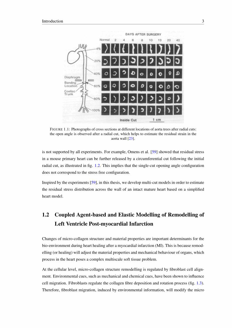
1.1 Photographs of cross sections at different locations of aorta trees after radialcuts: the open angle is observed after a radial cut, which helps to estimate theresidual strain in the aorta wall [23]. . . . . . . . . . . . . . . . . . . . . . . . 3
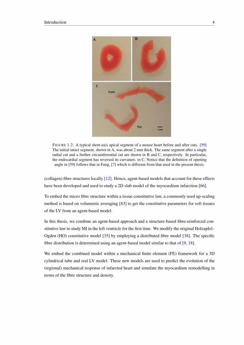
1.2 A typical short-axis apical segment of a mouse heart before and after cuts. [59]The initial intact segment, shown in A, was about 2 mm thick. The same seg-ment after a single radial cut and a further circumferential cut are shown in Band C, respectively. In particular, the endocardial segment has reversed its cur-vature, in C. Notice that the definition of opening angle in [59] follows that inFung, [7] which is different from that used in the present thesis. . . . . . . . . . 4
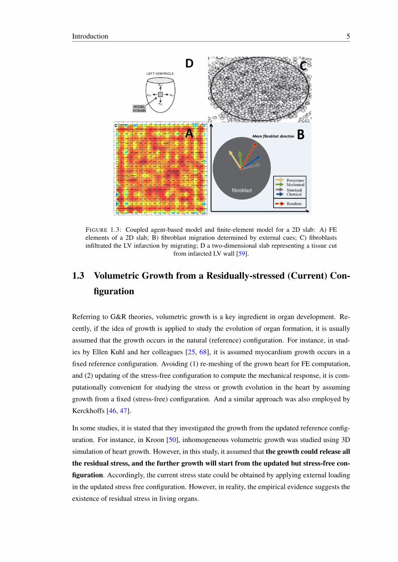
1.3 Coupled agent-based model and finite-element model for a 2D slab: A) FE el-ements of a 2D slab; B) fibroblast migration determined by external cues; C)fibroblasts infiltrated the LV infarction by migrating; D a two-dimensional slabrepresenting a tissue cut from infarcted LV wall [59]. . . . . . . . . . . . . . . 5
2.1 Change of basis (2D case): left, orthonormal basis ei to orthonormal basis e′j;right, orthonormal basis ei to oblique basis e′j. . . . . . . . . . . . . . . . . . . 10
2.2 The cumulative deformation and intermediate deformations. . . . . . . . . . . 132.3 The cumulative deformation with a series of intermediate deformations. . . . . 142.4 The polar decompositions of the deformation gradient: up, the left polar decom-
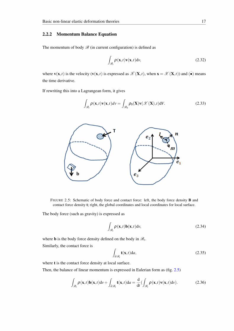
position; down, the right polar decomposition. . . . . . . . . . . . . . . . . . . 142.5 Schematic of body force and contact force: left, the body force density B and
contact force density t; right, the global coordinates and local coordinates forlocal surface. . . . . . . . . . . . . . . . . . . . . . . . . . . . . . . . . . . . 17
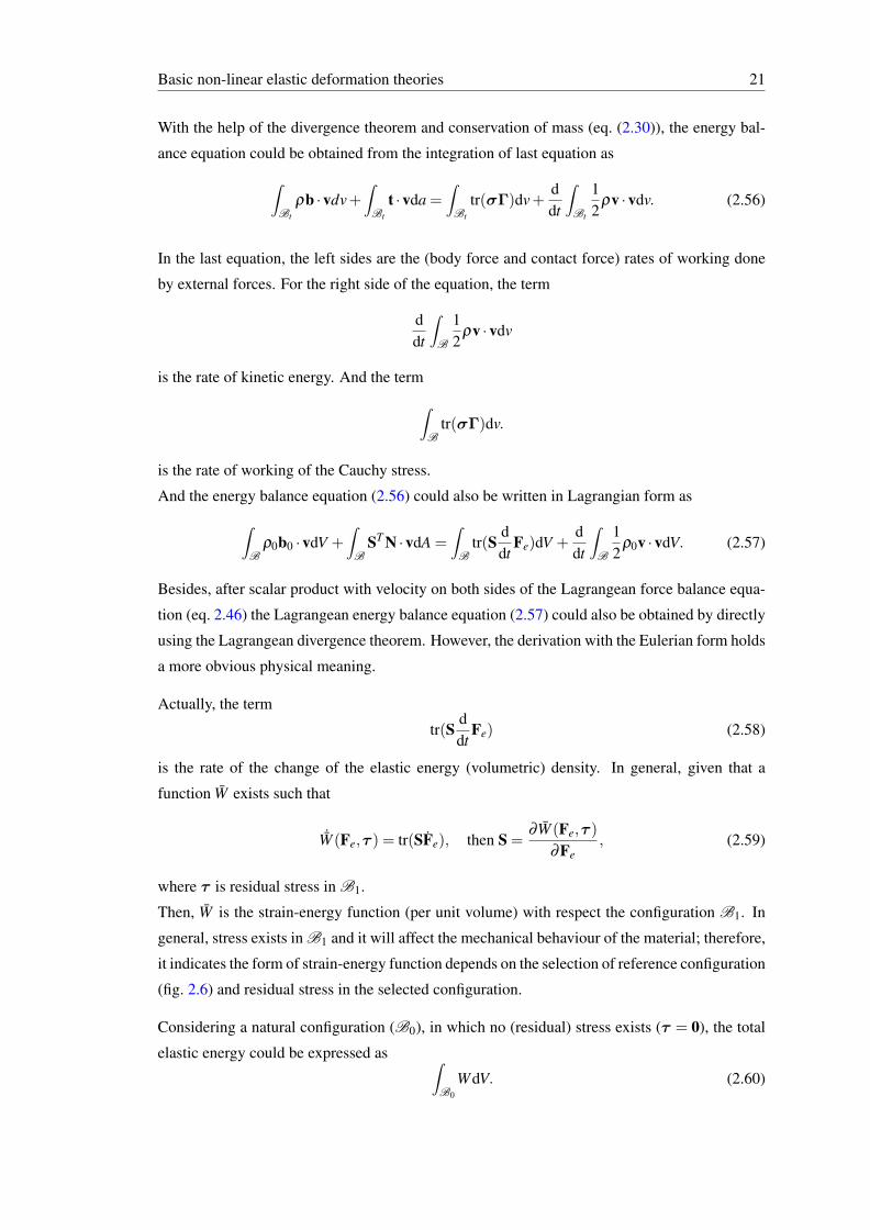
2.6 The strain energy function defined in an arbitrary configuration B1. B0 is thestress-free reference configuration, B1 is the residually-stressed configuration.The elastic deformation F2
e takes body into the current configuration B2 . . . . 222.7 The configurations for a mixture material with constituents k1 and k2. The two
materials are assumed to cover the same volume but with different volumetricfractions. . . . . . . . . . . . . . . . . . . . . . . . . . . . . . . . . . . . . . 25
2.8 The single-axis tension applied to a fibre-reinforced tissue with orthogonal fibrefamilies. . . . . . . . . . . . . . . . . . . . . . . . . . . . . . . . . . . . . . . 28
2.9 The comparison of Cauchy stresses from different SEFs: the comparison be-tween σx, dash line is σx obtained from SEF including the compressed fibre,solid line is σx obtained from SEF excluding the compressed fibre. . . . . . . . 31
3.1 Photographs of cross sections at different locations of aorta trees after cut ([23]). 343.2 Components of a healthy artery with three layers: intima (I), media (M), adven-
titia (A). . . . . . . . . . . . . . . . . . . . . . . . . . . . . . . . . . . . . . . 41
x
List of Figures xi
3.3 Configurations of arteries from constrained mixture model: left, the loadedconfiguration of arteries; middel, after unloading, the arteries deform into aresidually-stressed configuration; right, the radial cuts release the residual strainsin arteries measured by opening angle. . . . . . . . . . . . . . . . . . . . . . . 43
4.1 Configurations during the incremental growth: left, B0 is used as the fixed refer-ence, the incremental growth (Fg,i) updates the virtual stress-free configuration;right, the updated current configuration (Bg,2) is used as the stress-free one,where Cauchy stress is small (σg ≈ 0). . . . . . . . . . . . . . . . . . . . . . . 56
5.1 A typical short-axis apical segment of a mouse heart before and after cuts [59].The initial intact segment, shown in A, was about 2 mm thick. The same seg-ment after a single radial cut and a further circumferential cut is shown in B andC, respectively. In particular, the endocardial segment has reversed its curvature,in C. Notice that the definition of opening angle in [59] follows that in Fung, [8]which is different from that is used in the present paper. . . . . . . . . . . . . . 66
5.2 1-cut model: cylindrical model of the LV after a single radial cut of the intactunloaded configuration B3 into a stress-free sector B2. . . . . . . . . . . . . . 68
5.3 The 2-cut model: (a) cylindrical model of the LV as the intact ring in B3, (b)after a radial cut to B2, and (c) followed by a circumferential cut to B1. No-tice that the inner segment in B1 has a negative curvature, as in [59]. The redcurve, at the mid-wall radius R = (R(i)+R(o))/2 in (b), separates the inner andouter sectors which become the separate inner and outer sectors in B1 after thecircumferential cut. . . . . . . . . . . . . . . . . . . . . . . . . . . . . . . . . 70
5.4 The stress-free configuration B0 consisting of the four sectors obtained by cir-cumferential cuts of the two sectors in B1. . . . . . . . . . . . . . . . . . . . . 73
5.5 Fit of parameters of the HO model (5.1) to the experimental data (squares;from [61]) for the loading curves: The axial loading curve along fibre direc-tion (blue); the axial loading curve along cross-fibre direction (red). . . . . . . 76
5.6 The heterogeneous material parameters fitted to canine data from [56] (blacksolid lines). The red dashed lines indicate the constants used for the homoge-neous models, and the red solid lines are for the heterogeneous mice model. . . 77
5.7 Distribution of the residual stress components in the intact ring from (a) singlecut, (b) 2-cut, and (c) 4-cut models based on homogenous material assumption. 79
5.8 Distribution of the residual stress components from (a) single cut, (b) 2-cut, and(c) 4-cut models based on heterogeneous myocardium assumption. . . . . . . . 80
5.9 Residual stress distributions through the intima, media and adventitia of theartery wall as functions of the radial coordinate r, (a) without layer separation,and (b) the original result with layer separations from [36]. . . . . . . . . . . . 81
5.10 The change of shape of heart tube with shear stress σxy. . . . . . . . . . . . . . 825.11 The heart tube model with two symmetric fibre families: the dash line indicates
new fibres with fibre angle (−γ) to circumferential direction eθ . . . . . . . . . 835.12 Distribution of residual stresses components form: left, the symmetric fibre fam-
ilies; right, the single family . . . . . . . . . . . . . . . . . . . . . . . . . . . 865.13 Distribution of residual stresses components form: left, the symmetric fibre fam-
ilies; right, the single family. . . . . . . . . . . . . . . . . . . . . . . . . . . . 865.14 Two contacted material points at the interface of B2. A is the material point xA,
while B is the material point xB . . . . . . . . . . . . . . . . . . . . . . . . . . 875.15 The residual stress distributions in B2: left, the solution from stress continuity;
right, the solution from deformation continuity. . . . . . . . . . . . . . . . . . 885.16 No observable deformations occur after additional radial cuts [23]. . . . . . . . 89
List of Figures xii
5.17 Radial cut on 1-cut configuration: a radial cut at of 1-cut configuration B2. Theslice will deform into new configuration B′2. . . . . . . . . . . . . . . . . . . . 90
6.1 (a) The LV geometry with 28mm long axis, internal radius of 5mm and externalradius of 10mm at the base, and a block cut from the LV wall. The basis vec-tors at the reference configuration are (c0, l0, n0) for local coordinates, wherec0, l0, and n0 are the local circumferential, longitudinal and transmural unit vec-tors. The basis vectors at the reference configuration are (X, Y, Z) for globalCartesian coordinates, with origin O at the LV apex. (b) The fibre structurethrough the thickness of the LV wall. (c) Five longitudinal–circumferential sec-tions through the wall thickness. Collagen fibres lie in the c0–l0 plane. . . . . . 96
6.2 A) The resultant cue that represents the mean fibroblast direction is computedfrom a weighted combination of all cues; B) the von Mises distribution of thefibroblast orientation. . . . . . . . . . . . . . . . . . . . . . . . . . . . . . . . 100
6.3 The shadowed areas show the range of Σ of stretched collagen fibres within−π
2 < θ < π
2 for selected scenarios (dash line denotes I4 = 1): (a) case 1, C23 >0; (b) case 2, C33− 1 > 0,∆ ≤ 0; (c) case 2, C33− 1 > 0,∆ > 0; (d) case 2,C33−1 < 0,∆ > 0. . . . . . . . . . . . . . . . . . . . . . . . . . . . . . . . . 103
6.4 Flowchart of the coupled agent-based and FE LV model. . . . . . . . . . . . . 1066.5 The FE models of (a) a transmural circular cryoinfarct with r0 ≈ 5.5mm and
Xc = (10.12,2.82,0.81), and (b) a transmural elliptical cryoinfarct (with longaxix ≈ 15mm, short axis ≈ 5mm and Xc = (10.12,2.82,0.81), in the anteriorwall. . . . . . . . . . . . . . . . . . . . . . . . . . . . . . . . . . . . . . . . 107
6.6 Comparison of estimated infarct collagen volumetric evolutions with the mea-surements: the collagen volumetric fractions of infarcted tissues are calculatedthrough the remodelling processes of collagen fibre families via eq. 6.19. Then,the volume average of collagen fibre fractions among all infarcted tissues is em-ployed to describe the evolutions of the collagen fraction. The simulated results(blue for Circular MI and red for Elliptical MI) are compared with evolutions ofexperimentally-measured collagen fractions in [18] (black dots with error bars). 108
6.7 The evolution of collagen fibre structure for a circular MI: (a) – (e) 0–5 weeks;(f) the overlap of estimated fibre structure with the experimental measurements5 weeks post-MI [18]) . . . . . . . . . . . . . . . . . . . . . . . . . . . . . . 109
6.8 (a) The mean angle changes during the circular MI, (b) the kurtosis of the fibrestructure. . . . . . . . . . . . . . . . . . . . . . . . . . . . . . . . . . . . . . 110
6.9 The evolution of collagen structure at the epicardial surface of the circular in-farcted zone: The red arrow is the mean angel of overall fibre structure, whilethe blue arrows are the mean values of fibres of much smaller local pockets ofsize. . . . . . . . . . . . . . . . . . . . . . . . . . . . . . . . . . . . . . . . . 110
6.10 Evolution of the first principle stress distribution for the circular MI; its locationis indicated by the arrow. The bottom right is a 3D plot at 5 weeks post-MI. . . 111
6.11 The evolution of (a) radial stress; (b) circumferential stress; and (c) longitudinalstress, for the circular MI. . . . . . . . . . . . . . . . . . . . . . . . . . . . . . 111
6.12 Strain evolutions over time. (a): preferential accumulation in the circumferentialdirection reduced strain anisotropy. The predicted strain trends agreed reason-ably with the experimentally measured strains 6 weeks after cryoinfarction [18].
. . . . . . . . . . . . . . . . . . . . . . . . . . . . . . . . . . . . . . . . . . 1126.13 Fibre structure at 5 weeks post-MI, with (red solid) and without (red dashed) the
mechanical cue. The measured data are also shown as dashed line with error bars 113
List of Figures xiii
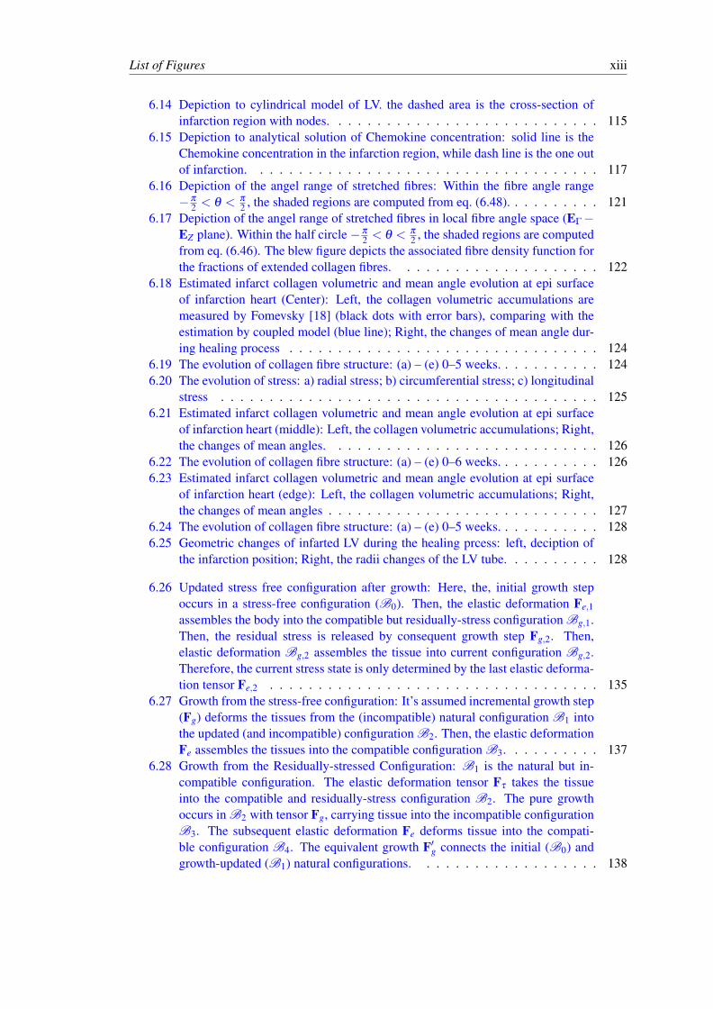
6.14 Depiction to cylindrical model of LV. the dashed area is the cross-section ofinfarction region with nodes. . . . . . . . . . . . . . . . . . . . . . . . . . . . 115
6.15 Depiction to analytical solution of Chemokine concentration: solid line is theChemokine concentration in the infarction region, while dash line is the one outof infarction. . . . . . . . . . . . . . . . . . . . . . . . . . . . . . . . . . . . 117
6.16 Depiction of the angel range of stretched fibres: Within the fibre angle range−π
2 < θ < π
2 , the shaded regions are computed from eq. (6.48). . . . . . . . . . 1216.17 Depiction of the angel range of stretched fibres in local fibre angle space (EΓ−
EZ plane). Within the half circle−π
2 < θ < π
2 , the shaded regions are computedfrom eq. (6.46). The blew figure depicts the associated fibre density function forthe fractions of extended collagen fibres. . . . . . . . . . . . . . . . . . . . . 122
6.18 Estimated infarct collagen volumetric and mean angle evolution at epi surfaceof infarction heart (Center): Left, the collagen volumetric accumulations aremeasured by Fomevsky [18] (black dots with error bars), comparing with theestimation by coupled model (blue line); Right, the changes of mean angle dur-ing healing process . . . . . . . . . . . . . . . . . . . . . . . . . . . . . . . . 124
6.19 The evolution of collagen fibre structure: (a) – (e) 0–5 weeks. . . . . . . . . . . 1246.20 The evolution of stress: a) radial stress; b) circumferential stress; c) longitudinal
stress . . . . . . . . . . . . . . . . . . . . . . . . . . . . . . . . . . . . . . . 1256.21 Estimated infarct collagen volumetric and mean angle evolution at epi surface
of infarction heart (middle): Left, the collagen volumetric accumulations; Right,the changes of mean angles. . . . . . . . . . . . . . . . . . . . . . . . . . . . 126
6.22 The evolution of collagen fibre structure: (a) – (e) 0–6 weeks. . . . . . . . . . . 1266.23 Estimated infarct collagen volumetric and mean angle evolution at epi surface
of infarction heart (edge): Left, the collagen volumetric accumulations; Right,the changes of mean angles . . . . . . . . . . . . . . . . . . . . . . . . . . . . 127
6.24 The evolution of collagen fibre structure: (a) – (e) 0–5 weeks. . . . . . . . . . . 1286.25 Geometric changes of infarted LV during the healing prcess: left, deciption of
the infarction position; Right, the radii changes of the LV tube. . . . . . . . . . 128
6.26 Updated stress free configuration after growth: Here, the, initial growth stepoccurs in a stress-free configuration (B0). Then, the elastic deformation Fe,1assembles the body into the compatible but residually-stress configuration Bg,1.Then, the residual stress is released by consequent growth step Fg,2. Then,elastic deformation Bg,2 assembles the tissue into current configuration Bg,2.Therefore, the current stress state is only determined by the last elastic deforma-tion tensor Fe,2 . . . . . . . . . . . . . . . . . . . . . . . . . . . . . . . . . . 135
6.27 Growth from the stress-free configuration: It’s assumed incremental growth step(Fg) deforms the tissues from the (incompatible) natural configuration B1 intothe updated (and incompatible) configuration B2. Then, the elastic deformationFe assembles the tissues into the compatible configuration B3. . . . . . . . . . 137
6.28 Growth from the Residually-stressed Configuration: B1 is the natural but in-compatible configuration. The elastic deformation tensor Fτ takes the tissueinto the compatible and residually-stress configuration B2. The pure growthoccurs in B2 with tensor Fg, carrying tissue into the incompatible configurationB3. The subsequent elastic deformation Fe deforms tissue into the compati-ble configuration B4. The equivalent growth F′g connects the initial (B0) andgrowth-updated (B1) natural configurations. . . . . . . . . . . . . . . . . . . 138
List of Figures xiv
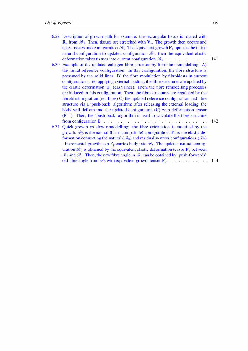
6.29 Description of growth path for example: the rectangular tissue is rotated withRe from B0. Then, tissues are stretched with Ve. The growth then occurs andtakes tissues into configuration B3. The equivalent growth Fg updates the initialnatural configuration to updated configuration B1; then the equivalent elasticdeformation takes tissues into current configuration B3 . . . . . . . . . . . . . 141
6.30 Example of the updated collagen fibre structure by fibroblast remodelling. A)the initial reference configuration. In this configuration, the fibre structure ispresented by the solid lines. B) the fibre modulation by fibroblasts in currentconfiguration, after applying external loading, the fibre structures are updated bythe elastic deformation (F) (dash lines). Then, the fibre remodelling processesare induced in this configuration. Then, the fibre structures are regulated by thefibroblast migration (red lines) C) the updated reference configuration and fibrestructure via a ‘push-back’ algorithm: after releasing the external loading, thebody will deform into the updated configuration (C) with deformation tensor(F−1). Then, the ‘push-back’ algorithm is used to calculate the fibre structurefrom configuration B. . . . . . . . . . . . . . . . . . . . . . . . . . . . . . . . 142
6.31 Quick growth vs slow remodelling: the fibre orientation is modified by thegrowth. B0 is the natural (but incompatible) configuration, Fτ is the elastic de-formation connecting the natural (B0) and residually-stress configurations (B2). Incremental growth step Fg carries body into B3. The updated natural config-uration B1 is obtained by the equivalent elastic deformation tensor F′τ betweenB1 and B3. Then, the new fibre angle in B1 can be obtained by ‘push-forwards’old fibre angle from B0 with equivalent growth tensor F′g. . . . . . . . . . . . 144
List of Tables
5.1 Transformation of the radii between configurations. . . . . . . . . . . . . . . . 755.2 Measured geometrical input for the 4-cut model, estimated from [59]. . . . . . 765.3 Computed intact ring from the homogeneous models, compared to measure-
ments [59]. . . . . . . . . . . . . . . . . . . . . . . . . . . . . . . . . . . . . 775.4 Computed intact ring from the heterogeneous models, compared to measure-
ments [59]. . . . . . . . . . . . . . . . . . . . . . . . . . . . . . . . . . . . . 785.5 Residual stress in the arteries computed using single-cut and original HO model [36] 81
6.1 fitted material parameters for myocardium from [61, 66]. . . . . . . . . . . . . 1046.2 Parameter values related to fibroblast dynamics and collagen remodelling. . . . 1086.3 Comparison of the mean stress at the infarct centre post-MI . . . . . . . . . . . 112
xv

Abbreviations
EDF Energy Density Function
FE Finite Element
G&R Growth and Remodelling
LV Left Ventricle
MI Myocardial Infarction
P-K Piola- Kirchhoff
SEF Strain Energy Function
xvi
Symbols
c distance vector
d normalized distance parameter
ei (or Ei) ith orthogonal basis
f fibre vector
g j (or G j) ith reciprocal basis
gi (or Gi) ith natural basis
k measurement of opening angle
m mass of body
n (or N) direction vector in current (reference) configuration
r (or R) radii of body
p Lagrange multiplier
q (or Q) survival rate of the living tissue
o (or o∗) observer
v velocity of material point
vi ith external cues for fibroblast migration
x (or x∗) vector of material point in specific configuration
B (or V ) specified configuration of body
C (b) right (left) Cauchy-Green tensors
C(•) chemokine concentration
Di j growth–rate coefficient
Dc diffusion coefficient
dS (or ds) the area vector in a specified configuration
E (e) Green (Lagrange) strain tensor
F (or A) deformation tensor
xvii
Symbols xviii
Fe elastic deformation tensor
Fg (or G) growth tensor
H(•) Heaviside function
I unit tensor
Ii ith invariance
I0 Bessel function of the first kind of order zero
M ( m) line element vector in reference (current) configuration
Mi weight factors for ith external cue
N(•) the number of collagen fibres
K First P–K stress
J determine of deformation tensor (volumetric ratio)
Pi ith rate parameter of fibroblast activation
R (or Q) rotation tensor
S nominal stress (tensor)
Scell value of the fibroblast migration speed
T (σ or σ∗) Cauchy stress
U & V positive definite symmetric (deformation) tensors
V (or v) volume of body
X (or X∗) vector of material point in reference configuration
W (•) SEF
Wi scaling factors for ith external cue
Γijk Christoffel symbol
Γ velocity gradient (tensor)
δi j Kronecker delta symbol
θ (or Θ) fibre angle
ϕ(•) fibre density function
Φ volumetric fraction
λ stretch
ρ density of body
ρ fibroblast resultant cue
σ2 variance
τ residual stress

Symbols xix
Ω boundary of region

To persons caring or cared for me.
xx
Chapter 1
Introduction
Living organs in human bodies continuously interact with in vivo bio-environment, while reshap-
ing and rearranging their constituents under chemical, mechanical or genetic stimuli through
their life cycles. During mature periods, these processes remain in a stable and homeostatic
state. However, changes of internal or external bio-environments will disrupt the balance, and
tissues will grow and remodel in response to an insult. For example, heart diseases will stimulate
the local healing process for myocardium remodelling. Besides, physiologically, exercise may
induce healthy and reversible growth and remodelling. After adjusting the growth (or turnover)
rates of constituents for living organs, they will develop volumetric and mass tissue changes to
adapt to the pathological or physiological changes in their bio-environment. From the perspec-
tive of biomechanics, changes in the bio-environment will induce the growth and remodelling
(G&R) process, which change the material properties of living organ by changing tissue struc-
ture. Then, the mechanical environment will be reset. Consequently, the mechanical cues will
feed back to the G&R processes. In the long run, the interaction between G&R and mechan-
ical response of living organs plays an important role in regulating the organ formulation or
pathological growth.
Therefore, to understand the interaction between the mechanical response and the G&R pro-
cess, an important ingredient in evaluating the involved mechanics is knowledge of the solid
mechanical properties of the soft tissues. Residual stress, resulting from G&R of soft tissues,
is important in modelling the mechanics of soft tissues, since the stress state in the reference
configuration has a substantial effect on the subsequent response to external loads, as illustrated
by the application of nonlinear elasticity theory. Thus, an appropriately estimated residual stress
at particular time instants could provide useful information about the growth history of living
tissues. However, how best to include the important effect of residual stress in cardiovascular
applications presents a modelling challenge.
1
Introduction 2
For G&R of living organs, changes of tissue structure and volume are important determinants
for organ development. This raises academic challenges for the understanding of the evolution
of material properties and mechanical response of living tissues within an dynamic environment.
For instance, the fibre structure in heart myocardium is remodelled by fibroblast migration, since
individual fibres are deposited and rotated by fibroblasts. To investigate the biomechanical re-
sponse of a organ during remodelling, complex multiple-scale calculations will be involved.
Besides, since remodelling is influenced by different environment cues (like chemical or me-
chanical cues), multi-physics calculations are also involved.
In this thesis, we focus on three new developments of soft tissue modelling. Firstly, a multiple
cut model is developed to estimate residual stress in the heart, which helps to explain recent ex-
periments on residual stress. Secondly, a multiscale three-dimensional heart model is developed
for simulating the remodelling process after heart infarction. This model captures the interaction
and information exchange processes between the mechanical behaviour and the collagen tissue
remodelling guided by bio-environmental cues. Finally, a volumetric growth approach is devel-
oped for simulating the inhomogeneous growth in residually-stressed current configurations of
living tissues.
1.1 Residual Stress and Opening-cut Method
To estimate the stress state in organs, traditionally, one of the fundamental ideas is to assume
the existence of a (stress-free) reference configuration [57], which coincides with the unloaded
configuration. However, according to experimental observation [23], the unloaded configuration
is not stress free, but is residually stressed. Obviously, residual stress affects the subsequent
mechanical response of the tissues to external loads. Therefore, it is of importance to estimate
the residual stress state in tissues. The residual stress can be estimated using the so-called
opening angle method [23], in which an opening angle indicative of the extent of the residual
strain can be measured after a single radial cut on intact arterial ring (fig. 1.1). Using the open-
angle configuration as the reference configuration, the residual stress of a cylindrical artery
model can be estimated [77]. This methodology has been extended to multiple cuts by Taber
and Humphrey [78], and used in the two-layered arterial models by Holzapfel et al. [34].
Residual stress in the reference configuration is important in modelling the mechanics of soft
tissues when using nonlinear elasticity theory to determine the stress state. And omission of the
residual stress leads to significantly different total stress predictions [71].
However, work that includes residual stress in complex organs, such as the heart, remains rare.
A few existing models for the left ventricle that take account of residual stress are based on the
assumption that a simple radial cut can release all the residual stresses [90], but this assumption
Introduction 3
FIGURE 1.1: Photographs of cross sections at different locations of aorta trees after radial cuts:the open angle is observed after a radial cut, which helps to estimate the residual strain in the
aorta wall [23].
is not supported by all experiments. For example, Omens et al. [59] showed that residual stress
in a mouse primary heart can be further released by a circumferential cut following the initial
radial cut, as illustrated in fig. 1.2. This implies that the single-cut opening angle configuration
does not correspond to the stress free configuration.
Inspired by the experiments [59], in this thesis, we develop multi-cut models in order to estimate
the residual stress distribution across the wall of an intact mature heart based on a simplified
heart model.
1.2 Coupled Agent-based and Elastic Modelling of Remodelling ofLeft Ventricle Post-myocardial Infarction
Changes of micro-collagen structure and material properties are important determinants for the
bio-environment during heart healing after a myocardial infarction (MI). This is because remod-
elling (or healing) will adjust the material properties and mechanical behaviour of organs, which
process in the heart poses a complex multiscale soft tissue problem.
At the cellular level, micro-collagen structure remodelling is regulated by fibroblast cell align-
ment. Environmental cues, such as mechanical and chemical cues, have been shown to influence
cell migration. Fibroblasts regulate the collagen fibre deposition and rotation process (fig. 1.3).
Therefore, fibroblast migration, induced by environmental information, will modify the micro
Introduction 4
FIGURE 1.2: A typical short-axis apical segment of a mouse heart before and after cuts. [59]The initial intact segment, shown in A, was about 2 mm thick. The same segment after a singleradial cut and a further circumferential cut are shown in B and C, respectively. In particular,the endocardial segment has reversed its curvature, in C. Notice that the definition of openingangle in [59] follows that in Fung, [7] which is different from that used in the present thesis.
(collagen) fibre structures locally [12]. Hence, agent-based models that account for these effects
have been developed and used to study a 2D slab model of the myocardium infarction [66].
To embed the micro fibre structure within a tissue constitutive law, a commonly used up-scaling
method is based on volumetric averaging [83] to get the constitutive parameters for soft tissues
of the LV from an agent-based model.
In this thesis, we combine an agent-based approach and a structure-based fibre-reinforced con-
stitutive law to study MI in the left ventricle for the first time. We modify the original Holzapfel–
Ogden (HO) constitutive model [35] by employing a distributed fibre model [38]. The specific
fibre distribution is determined using an agent-based model similar to that of [9, 18].
We embed the combined model within a mechanical finite element (FE) framework for a 3D
cylindrical tube and real LV model. These new models are used to predict the evolution of the
(regional) mechanical response of infarcted heart and simulate the myocardium remodelling in
terms of the fibre structure and density.
Introduction 5
FIGURE 1.3: Coupled agent-based model and finite-element model for a 2D slab: A) FEelements of a 2D slab; B) fibroblast migration determined by external cues; C) fibroblastsinfiltrated the LV infarction by migrating; D a two-dimensional slab representing a tissue cut
from infarcted LV wall [59].
1.3 Volumetric Growth from a Residually-stressed (Current) Con-figuration
Referring to G&R theories, volumetric growth is a key ingredient in organ development. Re-
cently, if the idea of growth is applied to study the evolution of organ formation, it is usually
assumed that the growth occurs in the natural (reference) configuration. For instance, in stud-
ies by Ellen Kuhl and her colleagues [25, 68], it is assumed myocardium growth occurs in a
fixed reference configuration. Avoiding (1) re-meshing of the grown heart for FE computation,
and (2) updating of the stress-free configuration to compute the mechanical response, it is com-
putationally convenient for studying the stress or growth evolution in the heart by assuming
growth from a fixed (stress-free) configuration. And a similar approach was also employed by
Kerckhoffs [46, 47].
In some studies, it is stated that they investigated the growth from the updated reference config-
uration. For instance, in Kroon [50], inhomogeneous volumetric growth was studied using 3D
simulation of heart growth. However, in this study, it assumed that the growth could release allthe residual stress, and the further growth will start from the updated but stress-free con-figuration. Accordingly, the current stress state could be obtained by applying external loading
in the updated stress free configuration. However, in reality, the empirical evidence suggests the
existence of residual stress in living organs.
Introduction 6
Besides, in the study by Ben Amar [3, 26], growth is assumed to occur in the current con-
figuration along the local principal directions. This assumption leads to a simplified growth
deformation tensor as Gi = diag(g1,g2,g3). Due to the geometric symmetry, the elastic defor-
mation tensor is also diagonal, since the living body was assumed as a sphere in this research.
Thus, the ith elastic deformation (gradient) tensor Fie = diag(λ1,λ2,λ3).
For the consequent G&R process, the overall deformation could be stated as
Ak = Gk ·Fke ·Gk−1 ·Fk−1
e · · ·G1 ·F1e ,
Ak = Fkg ·Fk
e ·Fk−1g ·Fk−1
e · · ·F1g ·F1
e ,
which, due to the symmetry of the growth and deformation tensors, could be rearranged as
Ak = Gk ·Gk−1 · · ·G1︸ ︷︷ ︸
overall growth
Fke ·Fk−1
e · · ·F1e .
Here, the contributions of a simplified growth law and the elastic deformation give an equivalent
growth in the fixed reference configuration. The overall growth tensor could directly update the
stress configurations. This approach is computationally convenient and avoids considering the
residual stress due to incompatible G&R processes in living organs, which makes it possible to
compute the stress from a stress-free configuration. However, living organs are actually exposed
to complex boundary conditions all the time, while the (volumetric) growth should occur from
the residually-stressed current configuration. This thesis tries to draw a sketch of how to cal-
culate the mechanical behaviour of soft tissue after introducing inhomogeneous growth in the
residually-stressed current configuration.
Introduction 7
1.4 Research Aims
Major research aims include to 1) develop a multiple-cut models to estimate the residual stress
in the LV; 2) develop a multiple-scale model to investigate the evolution of tissue structure and
mechanical behaviour of the heart during G&R processes of the LV after MI:
The details of aim (1) are presented as
Referring to previous researches, the residual stress is mostly estimated by a single-cut model
based on the ‘opening-angle’ approach. However, as a result of complex G&R processes in
living organs, distributions of residual stresses are more complicated. Inspired by the experi-
ments [59], multiple models are developed to estimate the residual stress distribution across the
wall of an intact mature heart based on a simplified heart model.
The details of aim (2) are presented as
a) The fibre structure and material properties will be significantly changed in the heart after MI.
At the cell level, those changes are regulated by fibroblast migration, which can be simulated
by an agent-based model. At the tissue level, the modified material response will change the
bio-mechanical environment of the LV and feed back to the G&R processes. In this paper, a
simple cylindrical model is used to study the evolution of the mechanical behaviour of the LV,
with certain biomechanical consequences for the infarcted LV.
Besides, for more reality, a 3D left ventricle model is developed within a finite element (FE)
framework to study the G&R process for an infarcted heart within a FE LV model coupled with
an agent-based fibroblast cell model.
b) Volumetric growth of the LV is another important factor affecting the heart formation process
and function. In previous research, the growth is assumed to occur in the fixed (and residual-
stressed) configuration. However, sustained growth actually occurs in the evolving current con-
figuration. A volumetric growth approach is needed to calculate the mechanical behaviour of
soft tissue after introducing inhomogeneous growth in the residually-stressed (current) configu-
ration.
1.5 Outline of Thesis
The basic theory of nonlinear elasticity is summarized in Chapter 2. Chapter 3 provides a review
of existing contributions to research with particular focus on 1) residual stress in soft tissues and

Introduction 8
the opening angle method, and 2) the interactions between the G&R process and the biomechan-
ical response of living organs. Multiple-cut models are developed in Chapter 4, and are used
to estimate residual stress distribution in the LV with respect to cut-induced configurations. To
investigate the evolution of the biomechanical environment and material properties of the heart
(tissues) after MI, an agent-based model, describing the fibroblast migration, is coupled with
an elastic LV model as a cylindrical tube and FE LV model (Chapter 5). The mechanism of
MI development is explained by these models in Chapter 6. A new approach is developed to
investigate inhomogeneous volumetric growth in the stressed (current) configuration in Chapter
7. Finally, limitations, conclusions and future works are discussed in Chapter 8. intro
Chapter 2
Basic Nonlinear Elastic DeformationTheory
In this project, the fundamental mathematical theory is ‘nonlinear elasticity’, which is suitable
for analyzing the material properties and mechanical behaviour of soft tissues. The basic con-
cepts about deformation and motions will be introduced in this section. Most of the attention
will be be paid to quasi-static problems, while the dynamic and time-dependent problems will
be only slightly touched on here.
The basic kinematics of deformation and motion will be described first. The concepts of stress
will be defined, as well as the stress equilibrium state (balance equations). The stress-deformation
relation will be given by the material constitutive laws. In this thesis, the strain energy function
(SEF), as a special form of constitutive law, is defined to describe the elastic behaviour of soft
materials. In general, the SEF can be defined in any arbitrary configuration, while the most pop-
ular way is to use the SEF referring to the natural (and stress-free) configuration. The general
form of SEF is used in this thesis. Besides, the SEF is also defined to describe soft tissues with
more than one constituent here.
2.1 Deformation and Strain
2.1.1 Observers and Frame of Reference
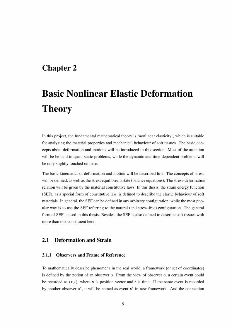
To mathematically describe phenomena in the real world, a framework (or set of coordinates)
is defined by the notion of an observer o. From the view of observer o, a certain event could
be recorded as (x, t), where x is position vector and t is time. If the same event is recorded
by another observer o∗, it will be named as event x∗ in new framework. And the connection
9
Basic non-linear elastic deformation theories 10
between x∗ and x is
x∗ = c(t)+Q(t)x, (2.1)
where c(t) is the distance vector, describing the observed position between two observers (c(t)=x∗−Q(t)x); Q is a tensor, transforming the vector observed by o into vector observed by o∗. If
two observers are under rectangular Cartesian coordinates, Q is an orthogonal tensor.
Transformation of basis: Normally, different observers will select different base to mathemati-
cally record the event. Now, we consider the basis for observer o to be ei and e′i (i=1,2,3)
for the second observer (o∗). Then, the transformation tensor Q could help to express the new
basis e′i respect to ei as
e′j = Qe j, (2.2)
i.e. if ei,
e′j
are basis for Cartesian coordinates, Qi j = e′j · ei ( j = 1,2,3).
Moreover, eq. (2.2) gives
cosθ′i j = e′i · e′j = Qei ·Qe j, (2.3)
where θ ′i j is the angle between e′i and e′j.
The change of the base could be expressed as
e′i⊗ e′j = Q ei⊗ e j QT . (2.4)
Assumingly here, we try to transform basis e′i back to basis ei, the expression could be similarly
obtained as
ei = QT e′i. (2.5)
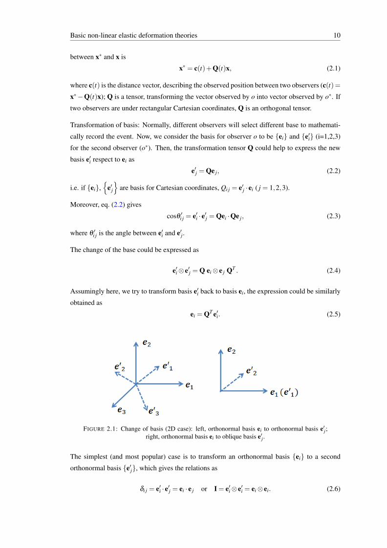
FIGURE 2.1: Change of basis (2D case): left, orthonormal basis ei to orthonormal basis e′j;right, orthonormal basis ei to oblique basis e′j.
The simplest (and most popular) case is to transform an orthonormal basis ei to a second
orthonormal basis e′j, which gives the relations as
δi j = e′i · e′j = ei · e j or I = e′i⊗ e′i = ei⊗ ei. (2.6)
Basic non-linear elastic deformation theories 11
where I is the unit tensor.
Application of eqs. (2.3), (2.4) and (2.6), it gives tensor Q as an orthogonal matrix, where
I = QQT and det(Q) =±1. (2.7)
It is worth to emphasize that eq. (2.7) of tensor Q is only valid for the transformation between
two orthonormal bases. In general cases, Q is not necessarily orthonormal.
2.1.2 Configuration and Deformation Gradient
To consider the relative deformation (and motion) of a ‘body’ with continuously distributed
material, the configurations should be pre-defined. A configuration is a one-to-one mapping to
describe the places occupied by all material points of body B. If suppressing the dependence of
deformation on time t, the position of material point X could be expressed as
x = X (X), (2.8)
where X is the one-to-one mapping of position in current configuration for material point X .
Considering the deformation from configuration B0 to B1, the differential on mapping X gives
dx = FdX and F = GradX (X) = OOO⊗X (X), (2.9)
where ‘Grad’ is the gradient operation with respect to X, and F is the deformation gradient.
Differential in curvilinear coordinate: In most previous researches, the differential operations
are analyzed in Cartesian coordinate, which is computationally convenient for the derivations.
However, in general, the differential operation should be analyzed in curvilinear coordinate,
while Cartesian coordinates are special cases of curvilinear coordinates with the fixed orthonor-
mal basis.
In the reference configuration, the natural basis vectors are defined as GI =∂X∂X I , while the
reciprocal basis is defined as GI(X) such that
δIJ = GI(X) ·GJ(X).
The gradient operator using reference coordinates is
Grad = GJ(∂/∂XJ).
Basic non-linear elastic deformation theories 12
In current configuration, the natural basis are defined as gi =∂x∂xi , while the reciprocal basis is
defined as gi(x) such that
δij = gi(x) ·g j(x).
The position vector in current configuration for material point X is expressed as
x = xigi(x) or x = xIGI, (2.10)
where the component xI is expressed as
xI = xiQiI,
and QiI are the components of the tensor Q (Qi
I = gi ·GI).
Recalling the gradient operator in the current coordinates and eq. (2.9), the deformation tensor
is obtained as
F = Grad (xIGI) = OOO⊗ (xIGI) =∂xI
∂XJ GI⊗G j + xI∂GI
∂XJ ⊗GJ, (2.11)
Introducing the Christoffel symbols as
∂GI
∂XJ =−ΓIJKGK and ΓK
IJ =∂GI
∂XJ ·GK =−GI ·
∂GK
∂XJ (2.12)
Inserting eq. (2.12) into (2.13), it yields
F =∂xI
∂XJ GI⊗GJ− (xIΓIJKGK⊗GJ). (2.13)
Eq. (2.13) is the general expression for deformation tensor from eq. (2.9). Considering the
deformation tensor is described within fixed Cartesian coordinates for current and reference
configurations, it gives the component of Christoffel symbols yields
Γki j = 0 and Q = I. (2.14)
Then,
F =∂xi
∂X j ei⊗E j. (2.15)
where ei and E j are the orthonormal basis vectors for the current and reference configurations,
respectively.
Basic non-linear elastic deformation theories 13
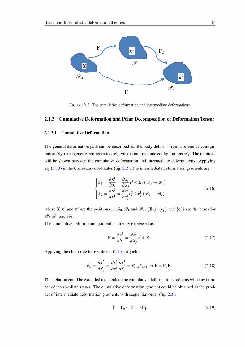
FIGURE 2.2: The cumulative deformation and intermediate deformations.
2.1.3 Cumulative Deformation and Polar Decomposition of Deformation Tensor
2.1.3.1 Cumulative Deformation
The general deformation path can be described as: the body deforms from a reference configu-
ration B0 to the generic configuration B2, via the intermediate configurations B1. The relations
will be shown between the cumulative deformation and intermediate deformations. Applying
eq. (2.13) in the Cartesian coordinates (fig. 2.2), The intermediate deformation gradients are
F1 =∂x1
∂X=
∂x1i
∂X je1
i ⊗E j (B0→B1)
F2 =∂x2
∂x1 =∂x2
i
∂x1je2
i ⊗ e1j (B1→B2),
(2.16)
where X,x1 and x2 are the positions in B0,B1 and B2; E j, e1i and e2
i are the bases for
B0,B1 and B2.
The cumulative deformation gradient is directly expressed as
F =∂x2
∂X=
∂x2i
∂X je2
i ⊗E j. (2.17)
Applying the chain rule to rewrite eq. (2.17), it yields
Fi j =∂x2
i
∂X j=
∂x2i
∂x1k
∂x1k
∂X j= F2,ikF1,k j ⇒ F = F2F1. (2.18)
This relation could be extended to calculate the cumulative deformation gradients with any num-
ber of intermediate stages. The cumulative deformation gradient could be obtained as the prod-
uct of intermediate deformation gradients with sequential order (fig. 2.3):
F = Fn · · ·F j · · ·F1, (2.19)
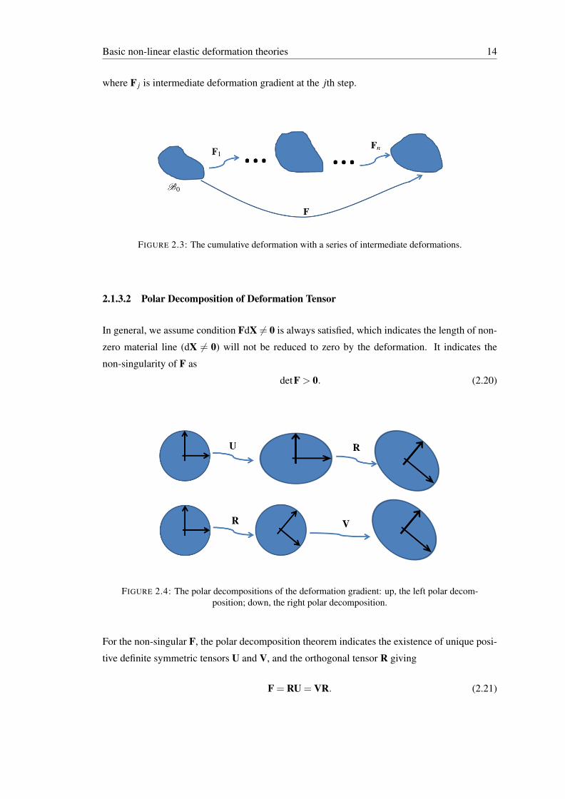
Basic non-linear elastic deformation theories 14
where F j is intermediate deformation gradient at the jth step.
FIGURE 2.3: The cumulative deformation with a series of intermediate deformations.
2.1.3.2 Polar Decomposition of Deformation Tensor
In general, we assume condition FdX 6= 0 is always satisfied, which indicates the length of non-
zero material line (dX 6= 0) will not be reduced to zero by the deformation. It indicates the
non-singularity of F as
detF > 0. (2.20)
FIGURE 2.4: The polar decompositions of the deformation gradient: up, the left polar decom-position; down, the right polar decomposition.
For the non-singular F, the polar decomposition theorem indicates the existence of unique posi-
tive definite symmetric tensors U and V, and the orthogonal tensor R giving
F = RU = VR. (2.21)
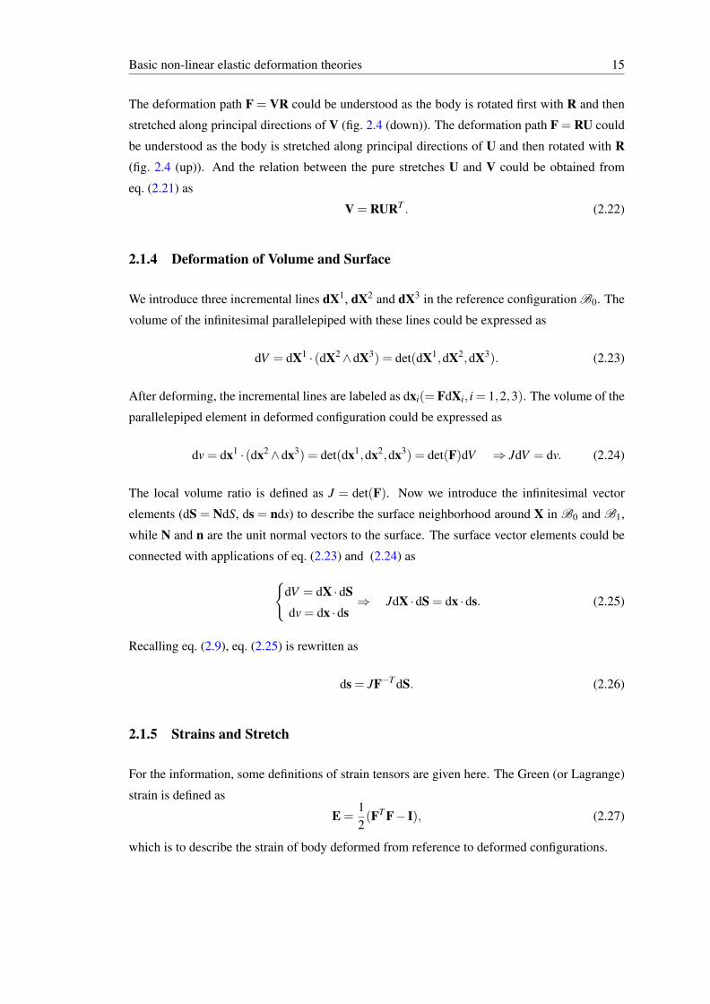
Basic non-linear elastic deformation theories 15
The deformation path F = VR could be understood as the body is rotated first with R and then
stretched along principal directions of V (fig. 2.4 (down)). The deformation path F = RU could
be understood as the body is stretched along principal directions of U and then rotated with R(fig. 2.4 (up)). And the relation between the pure stretches U and V could be obtained from
eq. (2.21) as
V = RURT . (2.22)
2.1.4 Deformation of Volume and Surface
We introduce three incremental lines dX1, dX2 and dX3 in the reference configuration B0. The
volume of the infinitesimal parallelepiped with these lines could be expressed as
dV = dX1 · (dX2∧dX3) = det(dX1,dX2,dX3). (2.23)
After deforming, the incremental lines are labeled as dxi(= FdXi, i = 1,2,3). The volume of the
parallelepiped element in deformed configuration could be expressed as
dv = dx1 · (dx2∧dx3) = det(dx1,dx2,dx3) = det(F)dV ⇒ JdV = dv. (2.24)
The local volume ratio is defined as J = det(F). Now we introduce the infinitesimal vector
elements (dS = NdS, ds = nds) to describe the surface neighborhood around X in B0 and B1,
while N and n are the unit normal vectors to the surface. The surface vector elements could be
connected with applications of eq. (2.23) and (2.24) as
dV = dX ·dSdv = dx ·ds
⇒ JdX ·dS = dx ·ds. (2.25)
Recalling eq. (2.9), eq. (2.25) is rewritten as
ds = JF−T dS. (2.26)
2.1.5 Strains and Stretch
For the information, some definitions of strain tensors are given here. The Green (or Lagrange)
strain is defined as
E =12(FT F− I), (2.27)
which is to describe the strain of body deformed from reference to deformed configurations.
Basic non-linear elastic deformation theories 16
The Eulerian strain is defined as
e =12[I− (FFT )−1] , (2.28)
which is to measure the strain from deformed to reference configurations.
Considering an arbitrary line element vector M in the reference configuration, it will deform
into element vector m in deformed configuration. The stretch of line element is written as
λ (M) =|m||M| =
(m ·m)1/2
(M ·M)1/2 = (M · (FT F)M
M ·M )1/2. (2.29)
2.2 Stress and Balance Laws
2.2.1 Conservation of Mass
In this thesis, masses of bodies are constant for observers with different velocities. Moreover,
if we don’t consider growth of the body, no new material will be added into B. Thus, the mass
function should be independent from t as
dm(B)
dt= 0,
which is called as the ‘mass conservation’.
In arbitrary configuration Bt , the mass density function ρ(x, t) could be defined as
m(Bt) =∫
Bt
ρ(x, t)dv.
Recalling the statement of mass conservation, the connection between density functions for
different configurations is expressed as
∫
Bt
ρ(x, t)dv =∫
B0
ρ0(X)dV, (2.30)
where ρ0 is the density function, dV is the local volume element, both independent of time t
and in reference configuration. If dV depends on t ( ∂
∂ t dV 6= 0), it indicates ‘mass conservation’
is not satisfied and body is growing. This case will be discussed in the section of ‘Volumetric
growth’.
Considering Bt is an arbitrary configuration, it suggests the connection of density (eq. (2.24))
is also valid for any sub-domain of Bt . Then, the relation between densities can be written as
ρ = Jρ0. (2.31)
Basic non-linear elastic deformation theories 17
2.2.2 Momentum Balance Equation
The momentum of body B (in current configuration) is defined as
∫
Bt
ρ(x, t)v(x, t)dv, (2.32)
where v(x, t) is the velocity (v(x, t) is expressed as X (X, t), when x = X (X, t)) and ˙(•) means
the time derivative.
If rewriting this into a Lagrangean form, it gives
∫
Bt
ρ(x, t)v(x, t)dv =∫
B0
ρ0(X)v(X (X), t)dV. (2.33)
FIGURE 2.5: Schematic of body force and contact force: left, the body force density B andcontact force density t; right, the global coordinates and local coordinates for local surface.
The body force (such as gravity) is expressed as
∫
Bt
ρ(x, t)b(x, t)dv, (2.34)
where b is the body force density defined on the body in Bt .
Similarly, the contact force is ∫
∂Bt
t(x, t)da, (2.35)
where t is the contact force density at local surface.
Then, the balance of linear momentum is expressed in Eulerian form as (fig. 2.5)
∫
Bt
ρ(x, t)b(x, t)dv+∫
∂Bt
t(x, t)da =ddt(∫
Bt
ρ(x, t)v(x, t)dv). (2.36)
Basic non-linear elastic deformation theories 18
The application of eq. (2.33) gives
ddt(∫
Bt
ρ(x, t)v(x, t)dv) =ddt(∫
B0
ρ0(X)v(X (X, t))dV
=∫
B0
ρ0(X)ddt
v(X (X, t))dV
=∫
Bt
ρ(x, t)ddt
vdv.
(2.37)
With help of eq. (2.37), eq. (2.36) is rewritten as
∫
t
ρ(x, t)b(x, t)dv+∫
Bt
t(x, t)da =ddt(∫
Bt
ρ(x, t)v(x, t)dv) =∫
Bt
ρ(x, t)ddt
vdv. (2.38)
2.2.3 Stress Tensors and Motions
2.2.3.1 Cauchy Stress Tensor
Cauchy′s theorem states that: the stress vector t(x) linearly dependent on the direction vector nand there therefore exists a second-order tensor field such that
t(x) = σ(x)n, (2.39)
where σ(x) is the Cauchy stress tensor.
Applying the balance of angular momentum, it indicates that the tensor of Cauchy stress is
symmetric, i.e.
σ = σT . (2.40)
(*the proof can be found in [57].)
Applying eq. (2.39), the linear balance equation could be rewritten as
∫
Bt
ρ(x, t)b(x, t)dv+∫
∂Bt
σn(x, t)da =∫
Bt
ρ(x, t)ddt
vdv. (2.41)
This is then rewritten by applying the divergence theorem as
∫
Bt
ρ(x, t)b(x, t)+divσT −ρ(x, t)ddt
vdv = 0. (2.42)
This equation is valid for arbitrary region B1, which indicates
ρb+divσT −ρddt
v = 0. (2.43)
Basic non-linear elastic deformation theories 19
2.2.3.2 Nominal Stress and Lagrangean Balance Equation
Recalling the relation between surface elements in different configurations (eq. (2.25)), the re-
sultant contact force of body b is written as
∫
∂Bt
σnda =∫
∂B0
JσF−T NdA,
where N is the normal vector of surface element in ∂B0.
Accordingly, the nominal stress (tensor) is defined as
S = JF−1σ. (2.44)
With the helps of eqs. (2.31), (2.37) and (2.44), the linear balance equation (2.45) is pushed back
into B0 as ∫
B0
ρ0(X)b0(X, t)dV +∫
∂B0
ST NdA =∫
B0
ρ0ddt
vdV, (2.45)
where b0 is the body force density in B0.
Application of the divergence theorem indicates
ρ0b0 +DivS−ρ0ddt
v = 0. (2.46)
Besides nominal and Cauchy stresses, another stress tensors are also widely used. For informa-
tion, the first and second Piola-Kirchhoff stresses are introduced here as
K = ST (first P-K stress), (2.47)
P = F−1K (second P-K stress). (2.48)
2.3 Constitutive Laws and Strain-energy Functions
2.3.1 Constitutive Laws
To analyze the motion of the body based on eqs. (2.43) or (2.46), we require to determine
the relation between stresses and motions. The constitutive law is generally used to describe the
mechanical behaviours of material, which can address the relation between stresses and motions.
In this project, only purely mechanical behavior will be focused, which implicitly indicates that
the thermodynamic variables don’t contribute to the material properties. In this thesis, only the
elastic behaviors will be discussed.
Basic non-linear elastic deformation theories 20
For a simple material, the stress could be solely determined by the motion history, which gives
the constitutive relation as
σ(x, t) = G(X t ;X , t), (2.49)
where G is the function to describe the constitutive relation relation, X t(X , t) is the motion
history as
X t(X ,s) = X (X , t− s) t ≥ s ≥ 0.
Concerning the constitutive law for an elastic material, the stress state could be directly deter-
mined by the deformation relative to an arbitrary reference configuration, with the helps of the
stress state in the reference configuration. Thus, for a uniform material, the constitutive law is
independent of material particle X . Therefore, the constitutive law could be written as
σ(x, t) = G(X ;Fe,τ ) ⇒ σ(x, t) = G(Fe,τ ). (2.50)
where τ is the Cauchy stress in the reference configuration, and Fe is the elastic deformation.
Considering the mechanical behaviours are observed by a new observer o∗ (eq. (2.1)), the de-
formation gradient and Cauchy stress could be rewritten with the helps of eqs. (2.2) and (2.9)
as
F∗e = QFe, σ∗ = QσQT . (2.51)
If the stress-deformation relation is unaffected by the selection of observer, eq. (2.51) gives
σ∗ = G(F∗e ,τ ). (2.52)
Applying eqs. (2.51) and (2.52), it gives
G(QFe,τ ) = QG(Fe,τ )QT . (2.53)
2.3.2 Strain-energy Function
The scalar product of eq. (2.43) with velocity v gives
ρb ·v+divσ ·v−ρ(ddt)v ·v = 0. (2.54)
This could be rearranged with the product rule of differentiation as
ρb ·v+div(σv)− tr(σΓ)−ρ(ddt
v) ·v = 0. (2.55)
where Γ is the velocity gradient as Γ= gradv(x, t), and ‘grad’ is gradient operation in the current
configuration with respect to x.
Basic non-linear elastic deformation theories 21
With the help of the divergence theorem and conservation of mass (eq. (2.30)), the energy bal-
ance equation could be obtained from the integration of last equation as
∫
Bt
ρb ·vdv+∫
Bt
t ·vda =∫
Bt
tr(σΓ)dv+ddt
∫
Bt
12
ρv ·vdv. (2.56)
In the last equation, the left sides are the (body force and contact force) rates of working done
by external forces. For the right side of the equation, the term
ddt
∫
B
12
ρv ·vdv
is the rate of kinetic energy. And the term
∫
Btr(σΓ)dv.
is the rate of working of the Cauchy stress.
And the energy balance equation (2.56) could also be written in Lagrangian form as
∫
Bρ0b0 ·vdV +
∫
BST N ·vdA =
∫
Btr(S
ddt
Fe)dV +ddt
∫
B
12
ρ0v ·vdV. (2.57)
Besides, after scalar product with velocity on both sides of the Lagrangean force balance equa-
tion (eq. 2.46) the Lagrangean energy balance equation (2.57) could also be obtained by directly
using the Lagrangean divergence theorem. However, the derivation with the Eulerian form holds
a more obvious physical meaning.
Actually, the term
tr(Sddt
Fe) (2.58)
is the rate of the change of the elastic energy (volumetric) density. In general, given that a
function W exists such that
˙W (Fe,τ ) = tr(SFe), then S =∂W (Fe,τ )
∂Fe, (2.59)
where τ is residual stress in B1.
Then, W is the strain-energy function (per unit volume) with respect the configuration B1. In
general, stress exists in B1 and it will affect the mechanical behaviour of the material; therefore,
it indicates the form of strain-energy function depends on the selection of reference configuration
(fig. 2.6) and residual stress in the selected configuration.
Considering a natural configuration (B0), in which no (residual) stress exists (τ = 0), the total
elastic energy could be expressed as ∫
B0
WdV. (2.60)
Basic non-linear elastic deformation theories 22
FIGURE 2.6: The strain energy function defined in an arbitrary configuration B1. B0 is thestress-free reference configuration, B1 is the residually-stressed configuration. The elastic
deformation F2e takes body into the current configuration B2
Assuming the elastic body deforms into B2 via the intermediate configuration B2, the relation
between deformation gradients could be given by application of eq. (2.18) as
F0e = F2
eF1e , (2.61)
where F0e is the elastic deformation gradient from B0 to B2, F1
e is the deformation gradient from
B0 to B1, and F2e is the deformation gradient from B1 to B2.
The application of elastic energy conservation gives
∫
B0
W (F0e)dV −
∫
B0
W (F1e)dV =
∫
B1
W (F2e ,τ )dv, (2.62)
This could be rewritten with the help of eq. (2.25) as
∫
B0
W (F0e)dV −
∫
B0
W (F1e)dV =
∫
B0
J1W (F2e ,τ )dV, (2.63)
where J1 = detF1e .
Since eq. (2.63) is valid for arbitrary volumes, it gives
W (F2e ,τ ) = (J1)
−1W (F0e)−W (F1
e). (2.64)
Referring to B0, the Cauchy stress in B2 is computed as
σ = J−10 F0
e∂W∂F0
e. (2.65)
Basic non-linear elastic deformation theories 23
Referring to B1 (eq. (2.64)), the Cauchy stress in B2 is computed as
σ = J−12 F2
e∂W∂F2
e= J−1
2 F2e
∂
∂F2eJ−1
1
[W (F0
e)−W (F1e)]. (2.66)
Obviously, W (F1e) and J1 are independent of F2
e , then
σ = J−12 J−1
1 F2e
∂
∂F2e
[W (F0
e)]. (2.67)
Application of the chain rule and eq. (2.61), then gives
σ = J−12 J−1
1 F2eF1
e∂
∂F2e
[W (F0
e)]= J−1
0 F0e
∂W∂F0
e= σ. (2.68)
2.3.2.1 Deformation Constraints
The elastic body sometimes will deform with local constraints, for example, the body is con-
strained to be inextensible in a certain direction. The constraint will mathematically reduce the
number of independent components of the elastic deformation tensor. For instance, a rigid rod
is assumed to be inextensible along its axial direction. The elastic deformation and energy will
be both zero along axial direction, no matter how huge the force is applied at both ends of the
rod.
We consider a deformation constraint to be defined by a scalar function
C(Fe) = 0. (2.69)
Then, the strain energy function with respect to B0 will be modified by the contribution of
constraints as
W (Fe,τ ,C) = W (Fe,τ )− pC(Fe), (2.70)
where p is a Lagrange multiplier.
Applying eq. (2.59), the nominal stress is given as
S =∂W (Fe,τ )
∂Fe− p
∂C∂Fe
, (2.71)
The application of the connection between Cauchy and nominal stresses gives
σ = J−1Fe∂W (Fe,τ )
∂Fe− pJ−1Fe
∂C∂Fe
, (2.72)
Basic non-linear elastic deformation theories 24
Considering the constraint is incompressibility of elastic body, it indicates constant volume of
body after elastic deformation), which gives the constraints function as
J(Fe)≡ 1 ⇒C(Fe) = J−1 = 0. (2.73)
Recalling the expressions of nominal and Cauchy stresses with constraints, they could be rear-
ranged as
S =∂W (Fe,τ )
∂Fe− p
∂ (J−1)∂Fe
=∂W (Fe,τ )
∂Fe− pF−1
e ,
(2.74)
and
σ = J−1Fe∂W (Fe,τ )
∂Fe− pI, (2.75)
where ∂J∂Fe
= JF−1e .
2.3.2.2 Strain Energy Function with Invariants
Recalling the definitions for the SEF for arbitrary configurations in eq. (2.64), it shows that
this SEF could be directly pushed back into the SEF of (fixed) stress-free configurations, even
though stress-free configuration does not really exist for particular bodies.
Considering the SEF for a stress-free configuration, it is a scalar function with respect to the
elastic deformation. Moreover, recalling the polar decomposition of the deformation gradient,
it suggests that the scalar function should be independent of rotation of elastic body and be
objective as
W (Fe) =W (RUe) =W (Ue) = W (λ1,λ2,λ3), (2.76)
where λi is the ith principal value of Ue (eq. (2.21)).
For an isotropic material, the mechanical responses are the same for deformation along arbitrary
directions, which indicates
W (λ1,λ2,λ3) = W (λ2,λ1,λ3) = W (λ3,λ2,λ1),
Furthermore, this could be represented with the invariants of the deformation tensor as
W (λ1,λ2,λ3) = Ψ(I1, I2, I3), (2.77)
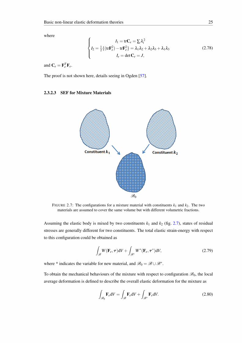
Basic non-linear elastic deformation theories 25
where
I1 = trCe = ∑λ 2i
I2 =12(trF2
e)− trF2e= λ1λ2 +λ2λ3 +λ1λ3
Ie = detCe = J,
(2.78)
and Ce = FTe Fe.
The proof is not shown here, details seeing in Ogden [57].
2.3.2.3 SEF for Mixture Materials
FIGURE 2.7: The configurations for a mixture material with constituents k1 and k2. The twomaterials are assumed to cover the same volume but with different volumetric fractions.
Assuming the elastic body is mixed by two constituents k1 and k2 (fig. 2.7), states of residual
stresses are generally different for two constituents. The total elastic strain-energy with respect
to this configuration could be obtained as
∫
BW (Fe,τ )dV +
∫
B∗W ∗(Fe,τ
∗)dV, (2.79)
where * indicates the variable for new material, and B0 = B∪B∗.
To obtain the mechanical behaviours of the mixture with respect to configuration B0, the local
average deformation is defined to describe the overall elastic deformation for the mixture as
∫
B0
FedV =∫
BFedV +
∫
B∗FedV. (2.80)
Basic non-linear elastic deformation theories 26
Then, the total elastic energy for mixture material is written as
∫
B0
W0(Fe)dV =∫
BW (Fe,τ )dV +
∫
B∗W ∗(Fe,τ
∗)dV. (2.81)
Applying eq. (2.80) and (2.81), the total elastic energy could be re-written as
∫
B0
W0(Fe)dV =∫
BΦW (Fe,τ )+Φ
∗W ∗(Fe,τ∗)dV, (2.82)
where Φ and Φ∗ are the volumetric fractions for materials (Φ+Φ∗ = 1).
Since this integration is valid for any volume, the SEF for the mixture is given as
W0(Fe) = ΦW (Fe,τ )+Φ∗W ∗(Fe,τ
∗). (2.83)
The state of residual stress will affect the mechanical behaviors of individual constituent. In
turn, it will influence the overall mechanical behaviors of the mixture body, which indicates
the importance of the residual stress in soft tissues to determine the mechanical behaviors of
mixture body under external loading. However, in a biomaterial mixture or living organ, the
residual stress is hard to determine, due to the complexity of its formation. For instance, living
tissues are usually composed by different constituents. The growth of different constituents are
usually incompatible. In turn, the residual stress will be induced by the deformations to get
the compatible configuration for living organ. Till now, how to accurately predict and measure
residual stress is still a open challenge for the study of the mechanical behaviours of living
organs.
Besides, the residual stress could also affect the expression of the SEF for the mixture. However,
for a mixture, the stress-free configuration usually doesn’t exist, while the individual stress-free
configurations exist for each constituent. If considering the mixture material as a whole body,
the stress-deformation relation could be given by the SEF for the mixture (eq. (2.83)) and could
be pushed into any arbitrary configuration.
Furthermore, the SEF for a body is given for n constituents as
W0 = ∑ΦiW (Fi
e,τi), (2.84)
where index i indicates variables for ith constituent and ∑i Φi = 1.
2.3.2.4 The SEF for a Fibre-reinforced Material
Considering the fibre-reinforced material, the fibres are embed into matrix materials, while the
interactions are ignored between fibres here. Moreover, it is assumed that fibres only contribute
to mechanical response along their axial directions. Then, the SEF for a fibre could be written
Basic non-linear elastic deformation theories 27
as
Wf (F fe ,τ f ) = Wf (λ f ,τ f ), (2.85)
where F fe is elastic deformation for fibre, λ f is stretch of fibre and τ f is residual stress.
The residual stress in fibres has been studied by many researches (e.g. Taber & Humphrey [78]).
In this section, the residual stress is assumed to be zero to reduce the complexity.
Applying eq. (2.29), then
λ f = (N · (FTe Fe)N)1/2, (2.86)
where N is the unit vector along fibre direction.
Application of eqs. (2.77), (2.80), (2.81) and (2.85), the SEF for a material reinforced by one
fibre family could be written as
W0(I1, I2, I3,λ f ) = ΦW (I1, I2, I3)+Φ∗W ∗(λ f ). (2.87)
Fiber dispersion in fibrous tissues has been recognized as being important in the mechanical
response of the tissue. Considering the 3-dimension fibre family, the orientation density function
ϕ(Θ,ϒ) could be defined to satisfy the normalization condition
∫∫
Ω
ϕ(Θ,ϒ)dΘdϒ = 1.
where Θ and ϒ are the spherical polar angles, and Ω = (Θ,ϒ) ∈ (0≤Θ≤ π,0≤ ϒ≤ 2π).
In this thesis, only the 2-dimension fibre family is used. Here, the 2-dimension orientation
density function (ϕ) is employed to describe the fibre structure
∫ϕ(Θ)dΘ = 1. (2.88)
where Θ is the fibre angle to the vector along mean direction of fibre family.
And the volumetric fraction for fibre family along a particular direction could be obtained as
Φ f
∫ϕ(Θ)dΘ, (2.89)
where Φ f is total volumetric fraction of fibres.
For a material with dispersed fibre families, the SEF could be given with the orientation density
function
W0(I1, I2, I3,λ f ) = ΦW (I1, I2, I3)+Φ f
∫ϕ(Θ)W ∗(λ f )dΘ, (2.90)
where Θ is the angle between fibre and certain directions in reference configuration, ϕ(Θ) is the
orientation density function.
In this project, the crosslinks and interactions between fibres are ignored. It is supposed that
fibres can not take compressive loads. To exclude the mechanical contributions of compressed
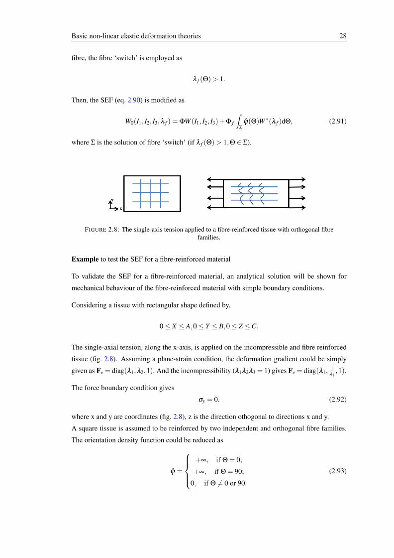
Basic non-linear elastic deformation theories 28
fibre, the fibre ‘switch’ is employed as
λ f (Θ)> 1.
Then, the SEF (eq. 2.90) is modified as
W0(I1, I2, I3,λ f ) = ΦW (I1, I2, I3)+Φ f
∫
Σ
ϕ(Θ)W ∗(λ f )dΘ, (2.91)
where Σ is the solution of fibre ‘switch’ (if λ f (Θ)> 1,Θ ∈ Σ).
FIGURE 2.8: The single-axis tension applied to a fibre-reinforced tissue with orthogonal fibrefamilies.
Example to test the SEF for a fibre-reinforced material
To validate the SEF for a fibre-reinforced material, an analytical solution will be shown for
mechanical behaviour of the fibre-reinforced material with simple boundary conditions.
Considering a tissue with rectangular shape defined by,
0≤ X ≤ A,0≤ Y ≤ B,0≤ Z ≤C.
The single-axial tension, along the x-axis, is applied on the incompressible and fibre reinforced
tissue (fig. 2.8). Assuming a plane-strain condition, the deformation gradient could be simply
given as Fe = diag(λ1,λ2,1). And the incompressibility (λ1λ2λ3 = 1) gives Fe = diag(λ1,1λ1,1).
The force boundary condition gives
σy = 0. (2.92)
where x and y are coordinates (fig. 2.8), z is the direction othogonal to directions x and y.
A square tissue is assumed to be reinforced by two independent and orthogonal fibre families.
The orientation density function could be reduced as
ϕ =
+∞, if Θ = 0;
+∞, if Θ = 90;
0, if Θ 6= 0 or 90.
(2.93)
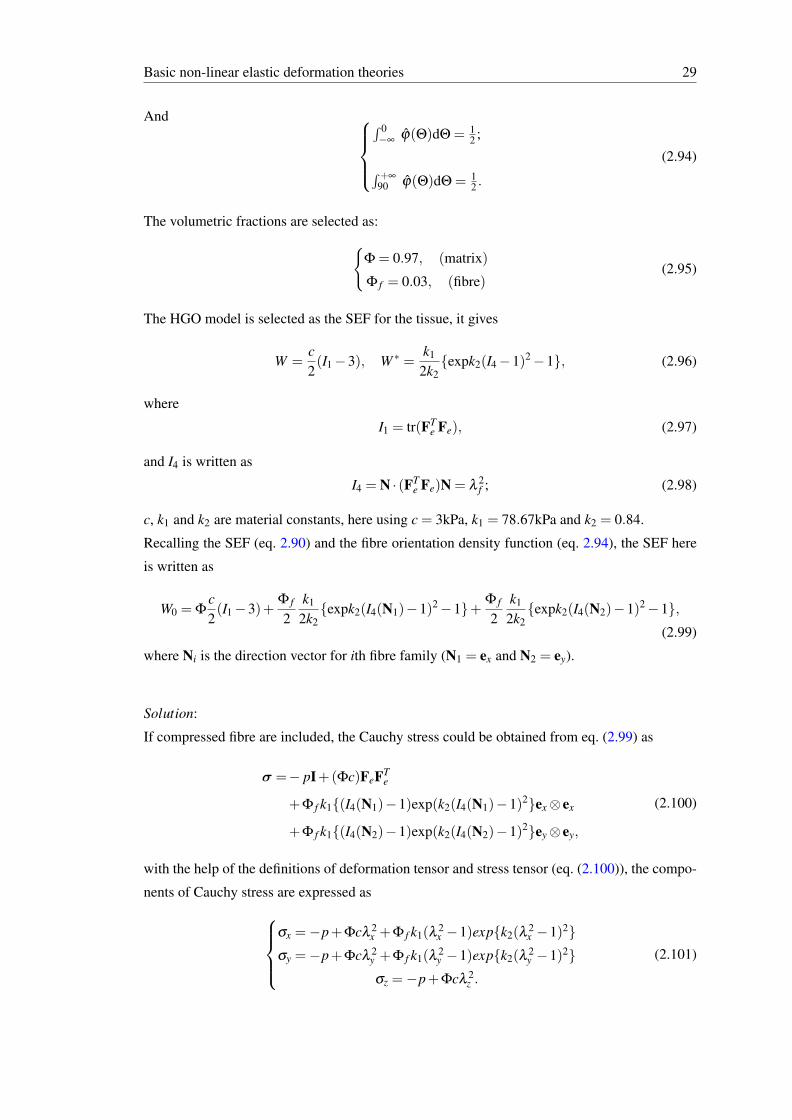
Basic non-linear elastic deformation theories 29
And
∫ 0−∞
ϕ(Θ)dΘ = 12 ;
∫ +∞
90 ϕ(Θ)dΘ = 12 .
(2.94)
The volumetric fractions are selected as:
Φ = 0.97, (matrix)
Φ f = 0.03, (fibre)(2.95)
The HGO model is selected as the SEF for the tissue, it gives
W =c2(I1−3), W ∗ =
k1
2k2expk2(I4−1)2−1, (2.96)
where
I1 = tr(FTe Fe), (2.97)
and I4 is written as
I4 = N · (FTe Fe)N = λ
2f ; (2.98)
c, k1 and k2 are material constants, here using c = 3kPa, k1 = 78.67kPa and k2 = 0.84.
Recalling the SEF (eq. 2.90) and the fibre orientation density function (eq. 2.94), the SEF here
is written as
W0 = Φc2(I1−3)+
Φ f
2k1
2k2expk2(I4(N1)−1)2−1+ Φ f
2k1
2k2expk2(I4(N2)−1)2−1,
(2.99)
where Ni is the direction vector for ith fibre family (N1 = ex and N2 = ey).
Solution:
If compressed fibre are included, the Cauchy stress could be obtained from eq. (2.99) as
σ =− pI+(Φc)FeFTe
+Φ f k1(I4(N1)−1)exp(k2(I4(N1)−1)2ex⊗ ex
+Φ f k1(I4(N2)−1)exp(k2(I4(N2)−1)2ey⊗ ey,
(2.100)
with the help of the definitions of deformation tensor and stress tensor (eq. (2.100)), the compo-
nents of Cauchy stress are expressed as
σx =−p+Φcλ 2x +Φ f k1(λ
2x −1)expk2(λ
2x −1)2
σy =−p+Φcλ 2y +Φ f k1(λ
2y −1)expk2(λ
2y −1)2
σz =−p+Φcλ 2z .
(2.101)
Basic non-linear elastic deformation theories 30
Recalling the boundary condition (eq. (2.92)), eq. (2.101)2 gives
σy = 0 ⇒ p = Φcλ2y +Φ f k1(λ
2y −1)expk2(λ
2y −1)2. (2.102)
With the help of the deformation tensor and boundary condition (2.102), the relations are ob-
tained from eq. (2.101) for ‘λx−σx’.
With help of eq. (2.98), I4(N1) = λ 21 ≥ 1 and I4(N2) = λ 2
2 ≤ 1, if applying single axis tension
along x axis. Therefore, if the compressed fibres are excluded (I4(N2) = λ 22 ≤ 1), the SEF could
be rewritten as
W0 = Φc2(I1−3)+
Φ f
2k1
2k2expk2(I4(N1)−1)2−1. (2.103)
If the compressed fibres are excluded by fibre switch (λ f > 1), the Cauchy stress could be
obtained from eq. (2.103) as
σ =− pI+(Φc)FeFTe
+Φ f k1(I4(N1)−1)exp(k2(I4(N1)−1)2ex⊗ ex,(2.104)
which gives
σx =−p+Φcλ 2x +Φ f k1(λ
2x −1)expk2(λ
2x −1)2
σy =−p+Φcλ 2y
σz =−p+Φcλ 2z .
(2.105)
Recalling the boundary condition (2.92), eq. (2.105)2 gives
σy = 0 ⇒ p = Φcλ2y . (2.106)
With the helps of the deformation tensor and boundary condition (2.106), the relations are ob-
tained from eq. (2.105) for ‘λx−σx’.
Fig. 2.9 shows the differences of mechanical behaviours between the SEF with and without the
fibre switch: the stresses, obtained from the SEF without fibre switch, are bigger. The differ-
ences are bigger with the increasing fibre stretch (λx). The results suggest that the stress predic-
tion is not accurate if the compressed fibres are not excluded. In this project, the fibre switchwill be included to describe the mechanical behaviours for fibre-reinforced materials.
2.4 Summary
In this section, the concepts of deformation and motions are explained. In general, the defor-
mation is to describe the shape change of a body respect to a certain configuration. Then, the
deformation gradient (tensor) is introduced to measure the changes of shape. From a perspective
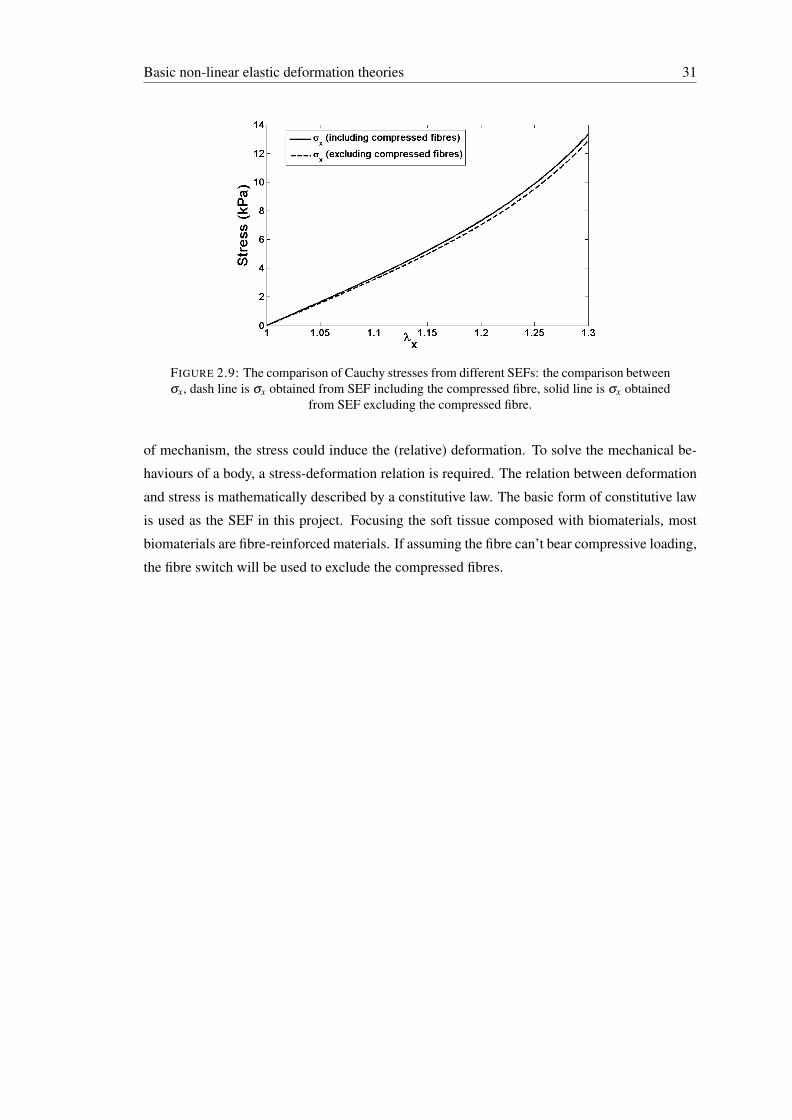
Basic non-linear elastic deformation theories 31
FIGURE 2.9: The comparison of Cauchy stresses from different SEFs: the comparison betweenσx, dash line is σx obtained from SEF including the compressed fibre, solid line is σx obtained
from SEF excluding the compressed fibre.
of mechanism, the stress could induce the (relative) deformation. To solve the mechanical be-
haviours of a body, a stress-deformation relation is required. The relation between deformation
and stress is mathematically described by a constitutive law. The basic form of constitutive law
is used as the SEF in this project. Focusing the soft tissue composed with biomaterials, most
biomaterials are fibre-reinforced materials. If assuming the fibre can’t bear compressive loading,
the fibre switch will be used to exclude the compressed fibres.
Chapter 3
Literature Review: Theories ofResidual Stress in Living OrgansEstimated by the Opening-angleMethod
A basic physical description is needed to understand and predict the mechanical behaviour of
soft tissues (or organs) in circulatory physiology. Generally, referring to small-deformation and
linear theories, the moduli of elasticity and Poisson’s ratios are originally employed to describe
the material properties for soft tissues, before the well-developed theories of large deformation.
However, in order to accurately describe the complex mechanical behaviours of soft tissue, large
deformation theories were introduced by researchers (like Bergel [6] or Fung [21]). Referring to
large deformation theories, the most popular method is to use the strain energy f unction (SEF)
or energy density f unction (EDF) to describe the material properties for soft tissue, which is
based on the laws of thermodynamics and the Gibbs-Duhem entropy inequality. At least to
the author, between nonlinear and linear theories, one of biggest differences is whether the
consequent mechanical behaviour of an elastic body is influenced by the stress states in the
reference configurations.
For nonlinear theories, the (natural) stress-free configuration is implicitly important to identify
the stress–deformation relation, even though the SEF could be defined with respect to the ar-
bitrary reference configuration. In the early stages of large deformation theories, the unloaded
configuration of soft tissues were selected as the stress-free one, which fact might introduce the-
oretical errors in estimating the mechanical behaviours of soft tissues or living organs if residual
stress exists in the selected configuration. This includes why the theories of residual stresses are
important.
32
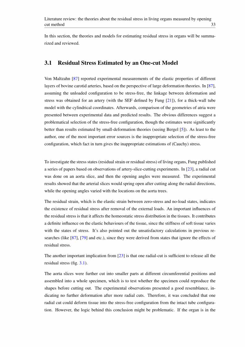
Literature review: the theories about the residual stress in living organs measured by openingcut method 33
In this section, the theories and models for estimating residual stress in organs will be summa-
rized and reviewed.
3.1 Residual Stress Estimated by an One-cut Model
Von Maltzahn [87] reported experimental measurements of the elastic properties of different
layers of bovine carotid arteries, based on the perspective of large deformation theories. In [87],
assuming the unloaded configuration to be stress-free, the linkage between deformation and
stress was obtained for an artery (with the SEF defined by Fung [21]), for a thick-wall tube
model with the cylindrical coordinates. Afterwards, comparison of the geometries of atria were
presented between experimental data and predicted results. The obvious differences suggest a
problematical selection of the stress-free configuration, though the estimates were significantly
better than results estimated by small-deformation theories (seeing Bergel [5]). As least to the
author, one of the most important error sources is the inappropriate selection of the stress-free
configuration, which fact in turn gives the inappropriate estimations of (Cauchy) stress.
To investigate the stress states (residual strain or residual stress) of living organs, Fung published
a series of papers based on observations of artery-slice-cutting experiments. In [23], a radial cut
was done on an aorta slice, and then the opening angles were measured. The experimental
results showed that the arterial slices would spring open after cutting along the radial directions,
while the opening angles varied with the locations on the aorta trees.
The residual strain, which is the elastic strain between zero-stress and no-load states, indicates
the existence of residual stress after removal of the external loads. An important influences of
the residual stress is that it affects the homeostatic stress distribution in the tissues. It contributes
a definite influence on the elastic behaviours of the tissue, since the stiffness of soft tissue varies
with the states of stress. It’s also pointed out the unsatisfactory calculations in previous re-
searches (like [87], [79] and etc.), since they were derived from states that ignore the effects of
residual stress.
The another important implication from [23] is that one radial-cut is sufficient to release all the
residual stress (fig. 3.1).
The aorta slices were further cut into smaller parts at different circumferential positions and
assembled into a whole specimen, which is to test whether the specimen could reproduce the
shapes before cutting out. The experimental observations presented a good resemblance, in-
dicating no further deformation after more radial cuts. Therefore, it was concluded that one
radial cut could deform tissue into the stress-free configuration from the intact tube configura-
tion. However, the logic behind this conclusion might be problematic. If the organ is in the
Literature review: the theories about the residual stress in living organs measured by openingcut method 34
FIGURE 3.1: Photographs of cross sections at different locations of aorta trees after cut ([23]).
stress-free configuration, any further cut will not introduce any further elastic deformation. This
logic is reasonable and rational. However, even if no further deformation occurs after the ad-
ditional cut, the organ could still be in residually-stressed configuration before the cut, while
the possible explanations could be: 1) a further cut is not sufficient to release the residual stress
from the one-cut configuration. If the residual stress distribution is symmetric and independent
of angular position, more radial cuts can not release any more residual stress. Therefore, in this
case, a radial cut does not induce elastic deformation from a residually-stressed configuration.
2) the organ went into a newly stressed configuration. For example, if the SEF is not mathemat-
ically convex.
Accurate biomechanical analysis is required to identify the stress-free configuration. The first
step is to experimentally quantify the residual strain for living organs. Before Omens [60], no
experimental measurement existed to identify the residual strain in heart tissue (myocardium).
Most peer researchers (like Huisman [42], or Yin [96]) used the unloaded configuration as the
stress-free configuration, and the results show the extraordinarily huge stress concentration at the
endocardial wall. In [60], the residual strain was measured and was used to recover a real stress-
free configuration, which could be expected to reduce the estimation of stress concentration at
the endocardial wall.
In the results of [60], the circumferential stretches were less than one at the endocaridal wall,
which indicated a compressive (residual) stress at the specified location. Therefore, this im-
portant feature could explain the huge stress concentration at the endocadial wall estimated by
the non-residual stress approach. Besides, additional deformation occurred after the second
cut, which indicates that the one-cut configuration is still a residually-stressed one for rat heart.
However, due to the obviously small magnitude of additional deformation, the stress-free con-
figuration could be represented by slices with one cut.
The radial cut and opening angle methods were applied to measure the residual strain in porcine
Literature review: the theories about the residual stress in living organs measured by openingcut method 35
and canine trachea (Han [28]). Results suggest that: (1) the opening angles were obviously
different in trachea induced by single radial cuts at different locations, especially for canine
trachea. It indicated the residual strains are not uniformly distributed in the trachea wall. (2)
The sections from anterior cuts, made by additional radial cuts, could represent the opening
angle configuration made by posterior cuts. It indicated that the additional cuts did not induce
more elastic deformation. And similar with conclusions on aorta or hearts ([28], [23], [60]), one
radial cut is sufficient to release all the residual stress. However, to the author, the statement
– one cut configuration is stress-free configuration– is not sufficiently proved due to the listed
reasons.
The residual strain could be generated by different growths ([28], [60], [23]). Then, the mea-
surements of the residual strain (by opening angle method), could relieve the information about
history of growth and heart formation. Besides the researches of residual strain in mature cardio-
vascular or heart systems, the changes of residual strain was speculated during the development
of embryonic heart ventricle [77]. In [77], the embryonic hearts were obtained from chicks at
different growth stages. The radial cuts were made to measure the residual strain in heart.
The results suggested that the opening angle decreased along with the heart formation [77]. For
the heart, the growth was faster in the outer layer of the myocardium. Besides, stress-driven
growth laws were proposed with explanations as: mechanical computation in [77] presented
that the peak stress occurred at the same location (epicardium) with highest growth rate, while
the strain peak was at endocardium; since living heart will never actually ‘know’ what are elastic
strains from the natural configuration, however, the stress in current configuration could be ‘felt’
by the heart. It supports that the growth is regulated by stress.
After (incompatible) growth, residual strain occurred in elastic body to keep the body continuous
without holes or overlaps in tissues. In [77], the stress-driven growth was proposed. Following
this idea, Rodiguez [65] introduced a continuum formulation to figure out the relation between
residual stress and stress-driven growth, with a simple tube model.
In [77], the relation between growth and stress was analyzed with a thick-wall heart model with
a simple growth tensor. For simple volumetric growth, the growth was assumed to occur in
the principal directions of the heart tube. With the diagonal growth tensor, the growth rate Ug
(represented in matrix form) and overall growth tensor Fg were defined as
Ug(t) =
Kx[Tzz(t)−T ∗zz] 0 0
0 Ky[Tzz(t)−T ∗zz] 0
0 0 0
⇒ Fg(t) =
∫ t
0Udt (3.1)
where Kx, Ky are the growth rate constants, Tzz is the axial stress, T ∗zz is the criteria value.
Literature review: the theories about the residual stress in living organs measured by openingcut method 36
In [77], it was suggested to explain how the residual stress might arise with incompatible growth
and how residual stress helps to reduce the stress concentration in the ventricular wall. Mean-
while, it indicates that growth and elastic deformations are decoupled during the continuous
growth. Moreover, the commutation law between growth and elastic deformation tensors was
implicitly included in [65] as
Feg = Fe,tnFg,tnFe,tn−1Fg,tn−1Fe,tn−2Fg,tn−2 · ··= Fe,tnFe,tn−1Fe,tn−2 · · · (Fg,tnFg,tn−1Fg,tn−2),
(3.2)
where Fe,tn , Fg,tn are the growth and elastic deformation tensors at time step tn
In this simple model with only diagonal deformation tensors, the commutation laws are suf-
ficient. However, this algorithm is problematic for the general case. For instance, for simple
shear, the commutation laws are not satisfied:
Fe =
1 λ 0
0 1 0
0 0 1
⇒ FeFg 6= FgFe. (3.3)
To better characterize the mechanical behaviours of arterial material, the constitutive framework
reference of Holzapfel, Gasser and Ogden (HGO) artery model was influenced. With the one-cut
and thick-wall model, the computations suggested some important advantages of HGO model,
compared with other models. Comparing with Delfino’s model, the HGO model gave better pre-
diction of the anisotropic mechanical behaviour in arteries. The HGO model could be applied
to more general cases than previous models (Vaishnav [82], Fung [22] and Takamizawa [79]).
For instance, those models are not always convex, then, the restrictions on material parameters
are required to avoid material instabilities, while the HGO model is convex.
The first attempt to mechanically model the residual stress and growth of developing embryo
heart was made by Taber [74]. Experiments were performed to measure the evolution of resid-
ual strain and the effects of the volume overload condition on the time course. The embryo chick
hearts were banded with nylon loops to introduce the overload condition. The results showed
the opening angles slightly decreased in the test group. However, the opening angles were sig-
nificantly lower after heart banding. With the observations of opening angle, the passive and
active zero-stress configuration could be identified (seeing stress equilibrium equation in [75]),
with both active and passive stress components.
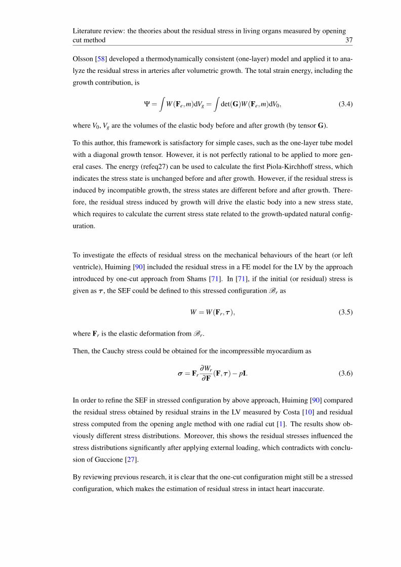
Literature review: the theories about the residual stress in living organs measured by openingcut method 37
Olsson [58] developed a thermodynamically consistent (one-layer) model and applied it to ana-
lyze the residual stress in arteries after volumetric growth. The total strain energy, including the
growth contribution, is
Ψ =∫
W (Fe,m)dVg =∫
det(G)W (Fe,m)dV0, (3.4)
where V0, Vg are the volumes of the elastic body before and after growth (by tensor G).
To this author, this framework is satisfactory for simple cases, such as the one-layer tube model
with a diagonal growth tensor. However, it is not perfectly rational to be applied to more gen-
eral cases. The energy (refeq27) can be used to calculate the first Piola-Kirchhoff stress, which
indicates the stress state is unchanged before and after growth. However, if the residual stress is
induced by incompatible growth, the stress states are different before and after growth. There-
fore, the residual stress induced by growth will drive the elastic body into a new stress state,
which requires to calculate the current stress state related to the growth-updated natural config-
uration.
To investigate the effects of residual stress on the mechanical behaviours of the heart (or left
ventricle), Huiming [90] included the residual stress in a FE model for the LV by the approach
introduced by one-cut approach from Shams [71]. In [71], if the initial (or residual) stress is
given as τ , the SEF could be defined to this stressed configuration Br as
W =W (Fr,τ ), (3.5)
where Fr is the elastic deformation from Br.
Then, the Cauchy stress could be obtained for the incompressible myocardium as
σ = Fr∂Wr
∂F(F,τ )− pI. (3.6)
In order to refine the SEF in stressed configuration by above approach, Huiming [90] compared
the residual stress obtained by residual strains in the LV measured by Costa [10] and residual
stress computed from the opening angle method with one radial cut [1]. The results show ob-
viously different stress distributions. Moreover, this shows the residual stresses influenced the
stress distributions significantly after applying external loading, which contradicts with conclu-
sion of Guccione [27].
By reviewing previous research, it is clear that the one-cut configuration might still be a stressed
configuration, which makes the estimation of residual stress in intact heart inaccurate.
Literature review: the theories about the residual stress in living organs measured by openingcut method 38
3.2 Residual Stress Estimated by a Multiple-cut Model
The growth of living tissues will induce residual stress in organs. In general, volumetric growth
and mass growth are two key approaches for analyzing the growth and remodelling process in
living organs. These two approaches will be reviewed about these two approaches.
3.2.1 Multiple-layer Model Using the Volumetric Growth Approach
In [88], after the radial cut, the bovine aorta was separated into the inner and outer layers by an
additional circumferential cut. The opening angles were different for the layers, which indicates
that residual stress and residual strains were different. This suggests using the two-layer model
to describe the mechanical behaviours of arteries [76].
Taber [76] applied the stress-dependent finite growth method and thick-wall heart tube model
for estimating the growth of aorta, with minor modifications of the model in [65]. Rather than
the one layer model in [65], the two-layer model was employed to represent the structure of the
aorta with both media and adventitia, which idea was inspired by the experimental observation
by Vossoughi [88].
In [88], it is assumed that growth is induced by the principal stress. Then, the stress-dependent
growth laws were used as
G(t) =
λg1 0 0
0 λg2 0
0 0 λg3
⇐ λgi = ∑Di jσi (3.7)
where σi is the ith principal stress, G is the growth rate tensor, Di j is the growth-rate coefficient
measured from experimental data. Referring to the last equation, the growth rate will be bigger
at material points with higher principal stress.
In previous experiments, the growth in bone was induced in the direction of stress, which guided
the choice of growth law (6.73). However, skeletal muscles were observed empirically to grow in
orthogonal directions to the primary stress [76]. To investigate the growth of aorta, two hypothe-
ses were proposed for future study about the stress-driven growth laws [76]: (1) strain-driven
law: the longitudinal growth was induced by strain along the associated strain directions, while
stress induces transverse growth orthogonal to the stress directions; (2) active stress-dependent
law: the active stress could induce the transverse growth. (The listed hypotheses were widely
used to study the growth of soft tissues. This will be further discussed in next section.)
To this author, one problem might arise from the calculation of stress equilibrium in [76]. In
general, in the multiple layer model, it is always required that the radial stress is continuous at
Literature review: the theories about the residual stress in living organs measured by openingcut method 39
the interface of contacted layers, which condition was ignored in [76]. For instance, in [39], the
stress continuity, ignored by [76], was described as
(σr|r=rm)+ = (σr|r=rm)
−, (3.8)
where rm is the radius of interface.
Recently, more experimental observations support to the non-homogeneous distribution of resid-
ual strain [63]. Later researchers have started to analytically investigate the residual stress and
opening angle in arteries with a multiple-layer model, while considering that the single-cut con-
figuration is residually stressed.
The two-layer and thick-wall tube model was employed by Taber [78]. The predicted opening
angles, produced by cuts at different locations, agreed well with experimental observations. This
supported the idea that the multiple cut model could be a good direction to analyze the residual
strain in arteries.
Compared to the heart function, the active stress in arteries is actually negligible. Taber [75] de-
veloped (passive) stress-driven laws to study the residual stress and evolution of vascular growth.
In previous experimental studies, it is supported that the growth of organs intends to restore the
wall stress and fluid shear stress into the stable states. Therefore, growth law, related with stable
stress states, is developed within the thick-wall tube model ([75]). In [75], predicted opening
angles matched well with experimental observations.
Though the non-homogeneous distributions of residual strains were accepted, early studies still
used the single cut model to estimate the stress distribution in the heart. Omens [59] made
the first attempt to experimentally measure the complex distributions of residual strain. The
rings of heart were cut from mature rats. A radial cut was first made on each heart. Then, a
circumferential cut was made to relieve another residual stress. The results show that additional
deformations were induced after the second cuts, which indicates 1) the one-cut configuration is
not the stress-free configuration; 2) the complex distribution of residual strains should be taken
into consideration for mechanical analysis of the heart tissue.
The finite element method is popular for developing a patient-specific computational model,
which is a powerful method for clinical diagnosis and treatment guidance. In analytical mod-
els, the residual stress (and opening angle) theories are accepted, while the effects of residual
stress were well explored for regulating the growth. However, FE models rarely take account of
both residual stress and growth in the study of the bio-mechanical behaviours of soft tissues or
living organs. The influence of residual stress had been numerically studied by Holzapfel [33]
on the physiological stress state of the arterial wall. In [33], the multiple layer structures of
Literature review: the theories about the residual stress in living organs measured by openingcut method 40
arteries were developed within a FE geometry, while the opening angles were used to compute
the residual stress states in arteries.
Alastrue [1] developed a patient-specific FE model to study adaptive volumetric growth, in
which the residual stress states were coupled in. Considering an arbitrary material point X in
the stress-free artery wall (with opening angle), the deformation F takes X into the compatible
configuration Br. After applying external loading at Br, the deformation Fe drives the material
point into the loaded configuration Bc, which gives the overall deformation as F = FeF0. In
other words, if starting from Br, it required to multiple the deformation with the deformation
associated with residual stress to compute the accurate mechanical response for arterial material
point. This is the basic idea how Alastrue [1] developed the FE model including residual stress
states. The deformation gradient was derivate from the cylindrical artery model with opening
angles. After applying pressure on the inner surface, Fr would be multiplied with further elastic
deformation to compute the stress states for arteries. The overall stress will be employed in
the stress-driven growth (from [73] with minor modifications) to simulate the diagonal growth
tensor. By repeating the growth-stress loop, the FE model could give the evolutions of stress
and adaptive growth with the patient-specific arterial geometry.
Ren [64] used the two-layer model to investigate the effects of growth on the stress distribu-
tion and deformation. The key features of the two-layer model and growth laws were similar
to these models in [78] or [34]: (1) the stress-driven growth laws and diagonal growth tensors
employed for each layer; (2) the active stress is generated by smooth muscle. To this author, the
key difference in [64] is the selection of the stress-free configuration. In previous studies, the
intact ring was used as the stress-free configuration, while the incompatible growth in different
layers would modify the stress-free configurations. However, in [64], the growth occurred in the
opened angle configuration as stress-free one, which will affect the stress distribution.
With better understanding of the structures of artery wall, the non-homogeneity of the wall struc-
ture is well accepted, and represented by three layers: intima, media and adventitia (fig. 3.2).
The fact that the residual strains (opening angles) were different in layers has been experimen-
tally demonstrated (Vossoughi [88], Han [29]). Rachev [63] measured the distribution of resid-
ual strains by the opening angle method for a multi-cut model. The first radial cuts were made
on the aorta slices of mature rats to introduce the opening angle. Then, the wall components
(collagen, elastin and smooth muscle) were grown chemically or thermally along the direction
from the inner wall to the outer wall or in the reverse direction. The changes of growth opening
angles were recorded to show the distribution of residual strains changing with time.
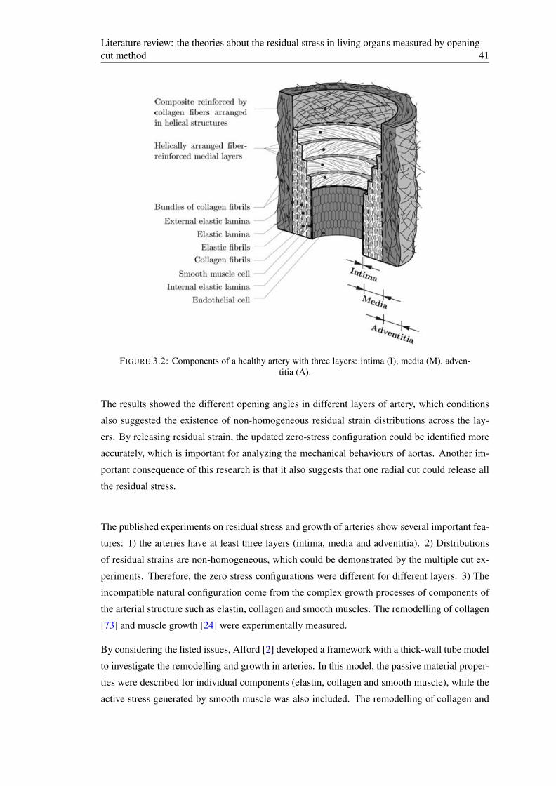
Literature review: the theories about the residual stress in living organs measured by openingcut method 41
FIGURE 3.2: Components of a healthy artery with three layers: intima (I), media (M), adven-titia (A).
The results showed the different opening angles in different layers of artery, which conditions
also suggested the existence of non-homogeneous residual strain distributions across the lay-
ers. By releasing residual strain, the updated zero-stress configuration could be identified more
accurately, which is important for analyzing the mechanical behaviours of aortas. Another im-
portant consequence of this research is that it also suggests that one radial cut could release all
the residual stress.
The published experiments on residual stress and growth of arteries show several important fea-
tures: 1) the arteries have at least three layers (intima, media and adventitia). 2) Distributions
of residual strains are non-homogeneous, which could be demonstrated by the multiple cut ex-
periments. Therefore, the zero stress configurations were different for different layers. 3) The
incompatible natural configuration come from the complex growth processes of components of
the arterial structure such as elastin, collagen and smooth muscles. The remodelling of collagen
[73] and muscle growth [24] were experimentally measured.
By considering the listed issues, Alford [2] developed a framework with a thick-wall tube model
to investigate the remodelling and growth in arteries. In this model, the passive material proper-
ties were described for individual components (elastin, collagen and smooth muscle), while the
active stress generated by smooth muscle was also included. The remodelling of collagen and
Literature review: the theories about the residual stress in living organs measured by openingcut method 42
elastin were mathematically described, as well as the growth laws for smooth muscle. For elastin
remodelling, it was assumed that the turnover rate is negligible. For collagen remodelling, It was
assumed that the old collagen is continuously replaced by new collagen. For smooth muscle,
the growth law is used as: the transverse growth is induced by passive stress, while the circum-
ferential growth is regulated by a combination of passive tensile and shear stresses, and active
strains. To solve a mechanical equilibrium problem, the governing equations were combined
with the previous intact ring model and radial cut slice model.
Besides the circumferential residual strains (measured by opening angles), the axial residual
strain was experimentally shown along longitudinal direction of aortas by Holzapfel ([39]), with
the axial strips taken from the anterior position of human aortas. After separating the layers from
axial strips, further axial deformations occurred, which demonstrated the axial residual strain.
In previous works (like [2]), the residual stress analysis was based on the opening angle method,
which does not account for address the 3D residual stress associated with both circumferential
and axial residual strains. Holzapfel and Ogden [36] constructed the first 3D model to analyze
the residual stresses in multiple layer arteries, considering axial bending.
The key difference from 2D residual stress model was the description of the elastic deformation
for media layer, which mathematically explained the deformation from the axial bending config-
uration into the circumferential bending configuration. With the help of stress equilibrium and
continuity of radial stresses at interface (3.8), the mechanical and geometric information could
be used to give the residual stress states in aortas.
The structure of an artery with atherosclerosis experimentally was observed with 5 layers: inner
intima, necrotic layer, outer intima, media and adventitia. Vandiver [85] analytically developed
a 5-layer model to study the growth formulation of an artery with atherosclerosis and studied
the effect of growth on peak stress. In [85], the stress-free configurations were unknown, which
would be determined from the pressurized artery tube and the residually-stressed configuration
with one radial cut. For a pressurized artery tube, the stress equilibrium equation is similar to
that in [23], while the continuous a displacement and radial stresses between layers are solved
with boundary conditions.
For a residually-stressed artery with an opening angle, the zero-net axial force and bending
moment conditions were applied. Then, the zero-stress configuration was solved after growth.
By considering different growth tensors, the effects on residual stress and peak stresses were
studied [85].
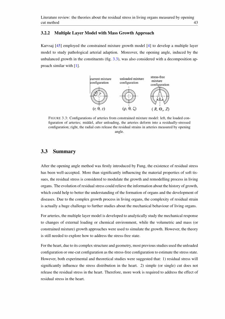
Literature review: the theories about the residual stress in living organs measured by openingcut method 43
3.2.2 Multiple Layer Model with Mass Growth Approach
Karvsaj [45] employed the constrained mixture growth model [4] to develop a multiple layer
model to study pathological arterial adaption. Moreover, the opening angle, induced by the
unbalanced growth in the constituents (fig. 3.3), was also considered with a decomposition ap-
proach similar with [1].
FIGURE 3.3: Configurations of arteries from constrained mixture model: left, the loaded con-figuration of arteries; middel, after unloading, the arteries deform into a residually-stressedconfiguration; right, the radial cuts release the residual strains in arteries measured by opening
angle.
3.3 Summary
After the opening angle method was firstly introduced by Fung, the existence of residual stress
has been well-accepted. More than significantly influencing the material properties of soft tis-
sues, the residual stress is considered to modulate the growth and remodelling process in living
organs. The evolution of residual stress could relieve the information about the history of growth,
which could help to better the understanding of the formation of organs and the development of
diseases. Due to the complex growth process in living organs, the complexity of residual strain
is actually a huge challenge to further studies about the mechanical behaviour of living organs.
For arteries, the multiple layer model is developed to analytically study the mechanical response
to changes of external loading or chemical environment, while the volumetric and mass (or
constrained mixture) growth approaches were used to simulate the growth. However, the theory
is still needed to explore how to address the stress-free state.
For the heart, due to its complex structure and geometry, most previous studies used the unloaded
configuration or one-cut configuration as the stress-free configuration to estimate the stress state.
However, both experimental and theoretical studies were suggested that: 1) residual stress will
significantly influence the stress distribution in the heart. 2) simple (or single) cut does not
release the residual stress in the heart. Therefore, more work is required to address the effect of
residual stress in the heart.
Chapter 4
Literature Review: Theories of Growthand Remodelling for Living Tissues
The interactions between living organs and the bio-environment play important roles in regulat-
ing pathological or physiological growth. In general, it has been experimentally demonstrated
that environmental factors, such as the chemical, mechanical or genetic stimuluses, could induce
growth and remodelling (G&R) processes in living organs. For instance, nutrition concentration
will be increased around the tumors, which helps to accelerate cell division and lead to the local
growth of tumors at the tissue level (chemical factors). In [76], the experiments show that the
myocardium will grow along the direction of principal tensile stress (mechanical factors). Dur-
ing the heart formation, the embryo heart will continuously and instinctively develop the heart
structure (genetic factor).
Living organs can re-shape themselves and reset the growth (or turnover) rates of their con-
stituents; in the long run, they will develop volumetric and mass changes to adapt to the patho-
logical or physiological changes in the bio-environment. G&R processes have been observed
in different patterns: For embryonic or young organs, they will continuously re-structure them-
selves to develop specified functions, like heart formation. For mature organs, they are expected
to stay in a relatively stable living state and serve as fully functional; however, pathologically, the
dynamic impact of bio-environmental changes will induce a quick remodelling process to reno-
vate the functional tissue. For instance, chronic disorder could develop maladaptive G&R, such
as the hypertrophic ventricular growth induced by systemic hypertension in the heart; physi-
ologically, body exercises will stimulate reversible growth to strengthen the functions of the
living organs. As evidence, the wall-thickness of artery is increased (in other words, eccentric
ventricular growth were observed) for animal after more body exercises, which could promote
muscle contractions.
44
Literature review: Theories of Growth and Remodelling for Living Tissues 45
After G&R, the functions and life cycles would be modified in living organs. However, the prin-
ciples governing those mechanism are still not fully understood that could address the relation
between external stimuli and growth processes. Obviously, improving the knowledges in this
particular field will give huge potential for the design and optimization of clinical treatments
to efficiently save more lives. However, in this relatively new field, many challenges exist.
As mentioned, the stimulus could be considered as the combined effects of different sources,
including mechanical, thermal, electrical and genetic information. These stimuli will simultane-
ously contribute to the successive growth processes in living organs. In practice, this fact raises
the complexity of figuring out the contributions of individual environmental factors. Besides,
to understand growth in living organs, the theoretical framework is expected to be based on the
coupling factors from multidisciplinary, which is still a gap in the current stages of knowledge.
For the biomechanical or even the mechanical community, the key questions now are: how could
the mechanical behaviours of soft tissues be mathematically described? what is the role played
by mechanical factor in the regulation of the growth? How would the mechanical functions and
behaviours of living organs be modified after the growth? How would the mechanical informa-
tion feedback and regulate changes of bio-environment during the life cycle? How would the
mechanical information be decoupled and coupled with information from other fields to regulate
the growth in living tissues?
Recently, significant improvements have been made to build up knowledge about the mechani-
cal behaviour of soft tissues, like theories of the nonlinear elastic deformations. To answer these
questions, in early stages of researches in this field, the mechanical stimuli was exclusively ex-
tracted. If controlling other stimuluses stable and unchanged, by recording the mechanical stim-
ulus and subsequent growth, the relations could be mathematically described between growth
and mechanical information. In the coming sections, the (mainstream) academic works will be
reviewed to show the current research stage and potential directions in this field.
It should be clarified that only two key categories about growth and remodelling will be ad-
dressed in those sections: (1) the remodelling of fibre-reienforced material; (2) the volumetric
and mass growth in living organs. These are closely related with author’s research interests,
4.1 Remodelling of (Collagen) Fibre-reinforced Soft Tissues
Considering the formations of living organs, if ignoring other stimuli (like chemical factors),
mechanical environment plays an important role for the adaptation of tissues. In other words,
the structure and functionality of soft tissues will be structured and optimized to adapt external
(mechanical) working environments.
Literature review: Theories of Growth and Remodelling for Living Tissues 46
Strain and stress are key indicators for measuring the load level in living organs. Experimental
evidence suggests strains and stresses are the mechanical factors inducing adaptations in tissues.
For instance, Huiskes [41] found that the strains could contribute to the bone growth. Taber [78]
hypothesized the stress-regulated growth in soft tissue. Later researchers studied how these
factors affect the fibre architecture.
Strain−driven f ibre remodelling
In [14], Driessen et. al. investigated the interrelations between collagen structure and mechani-
cal conditions in arteries via a strain-driven law, with an algorithm introduced in [13, 15]. After
applying abnormal loading (hypertension), the elastic deformation is obtained via the constitu-
tive laws of the artery wall. Then, the principal strains are obtain. The fibres are assumed to be
re-oriented to the directions of the principal strains in the current configuration as
dθ
dt= k(1− ft · ep) (4.1)
where dθ/dt is the rate of reorientation from fiber direction to the positive principal strain di-
rection (ep), , ft is the fibre orientation in the current configuration at time t.
In a time incremental ∆t, with helps of rotation tensor R, the new fibre orientation is given as
ft+1 = R(∆θ ,er)ft ,
where R is the rotation tensor based on ∆θ and the normalized rotation axis er.
After the fibre rotations by strain, the fibre is pushed back into the unloaded (and natural) con-
figuration, according to
f0,t+1 =F−1ft+1
||F−1ft+1||, (4.2)
where F is the elastic deformation gradient from the initial reference configuration to the current
configuration, f0,t+1 is the new orientation of a fibre in updated stress-free configuration.
After the fibre architecture is updated by previous process, the loaded configuration is re-
computed with the same loading boundary conditions. Repeating this iterative process, the
final fibre architecture is obtained till the reorientation of the fibre converge to a stable stage.
Actually, ultimately, the fibre orientations will perfectly align with the directions of principal
strains, which agrees with experimental observation.
Stress−driven f ibre remodelling
The stress is considered as the driving force for fibre remodelling in some researches (for exam-
ple, in [78]). Following this hypothesis, Hariton [31] used a thick-wall tube to simulate the fibre
reorientations in an artery wall via the stress-driven approach. After applying external loading
for an artery wall, the fibre is reoriented in the current configuration by a stress-driven law.
Literature review: Theories of Growth and Remodelling for Living Tissues 47
The new fibre orientations in remodelling-updated natural configuration could be obtained by the
push-back algorithm similar with eq. (4.2). Then, after the boundary-value problem is solved,
the fibre angles is deduced again. The final fibre structure would be obtained by repeating the
iteration till the stress field in the artery is stable. The computational results show the predicted
fibre structure also agrees with experimental observation.
The stress-driven law and algorithm were also applied to predict the fibre structures at the carotid
bifurcation by Hariton, which also gave the reasonable results comparing with experimental
data [17].
Summary
Actually, the previous stimulations mentioned in this subsection are more like the mathemat-
ical calculations to determine the optimal fibre structure when bearing the external load. The
important implications include: (1) the mechanical factors could be employed to explain the
remodelling in soft tissues. (2) it demonstrates that the living organs would optimize the fibre
structure responding to mechanical-biological environment. (3) In an artery, the fibre structures
simulated by stress-driven [31] or strain-driven [14] laws were similar and both relatively agree
with experimental data. It also suggested that the stress and strain distributions were coupled or
coaxial in arteries in some level.
4.1.1 G&R Process for Fibre-reinforced Tissues (from Cell Level to Tissue Level)
Fibre structure is the key feature for determining the mechanical behaviours of soft tissues.
In the real bio-environment, G&R processes are really complex and are usually induced by
environmental factors. In general, the fibres will be produced and removed by the fibroblasts.
Besides, the existing fibre alignments will be modulated or rotated by fibroblasts as well. Many
researchers have focused on what factors influence the activities of fibroblasts and how the
fibroblast activities regulate the fibre structure.
Due to the features of the fibre structure, different assumptions are introduced to describe the
material properties of collagen fibres: (1) the collagen fibre is considered as the ‘rope’ in the
tissue and doesn’t bear the compressive loading. For instance, Holzapfel et. al. [38], [37] used
the angular integration (AI) model to describe the mechanical behaviours of the fibre structure,
with a switch to properly exclude the influence of compressed fibres. Assuming the dispersed
fibre structure is defined by the fibre orientation density function ρ(θ), the angle range (Σ) of
stretched fibre could be determined by the fibre invariance as
I4(θ) = N · (CN)> 1⇒ θ ∈ Σ (4.3)
Literature review: Theories of Growth and Remodelling for Living Tissues 48
where C is the right Cauchy-Green deformation tensor, Σ is the solution for the inequity I4 > 1.
For the deformation C, the compressed fibres are excluded if I4 < 1.
(2) Actually, the crosslinks between collegan fibres were experimentally observed in many re-
searches (seeing [81]). However, the crosslinks suggested the higher fibre alignment and the
interactions between fibres, while it was usually assumed that the fibre responded independently
to external loading in previous studies (like [38]). By effects of fibre connections, the entire
fibre structure could bear compressive loading, though the individual fibre might not take any
compression.
In [49], Kroon used a new SEF to describe the mechanical behaviours of the fibre structure under
compressive or tensile loading. If ignoring the crosslinks between fibres, the fibre would act like
the ’rope’ and don’t take any compressive loading. As results, the mechanical contributions of
compressed fibres should be removed ([38]). However, with helps of cross-links, the tissue will
exhibit a certain stiffness in compression direction as well. Then, the SEF is introduced as
Ψ =kc
4a
∫ρexp(a(I4−1)2−1) ·H(I4−1)dΩ+
kcn4
∫ρ(ξc− I4)
2 ·H(ξc− I4)dΩ, (4.4)
where Ω is the angle domain in which the orientation density function ρ is defined. Constants
of kcn, kc and a are material parameters, I4 is the stretch along fibre (I4 = f · (Cf)). ξc is the
stretch of matrix material along M direction (ξc = C : A and A = FM/|FM|⊗FM/|FM|); F is
the related elastic deformation tensor; H(x) is the Heaviside step function.
The SEF (eq. 4.4) includes the contributions from fibres in tension (first term) and the matrix
material with compressed fibres (second term).
Moreover, accordingly, the crosslinks and interactions between fibres could be modulated by
the fibroblasts ([62]). Kroon [49] studies the remodelling process of the fibre structure, with the
mentioned constitutive law of soft tissue (eq. 4.4). Results suggest that the fibre orientations and
alignments are key features for soft tissues.
After re-structuring the fibre structure in the current configuration, the push-back method [31]
was also employed to determine the fibre network in the reference configuration. Interestingly,
the remodelling process in [49] ignored fibre degradations. For instance, after remodelling, the
orientation density function ρ will be updated. Meanwhile, the overall mass of fibres is changed,
which is indicated by the changing mass production rate. Besides, while the volumetric fraction
of fibres was implicitly ignored in this research. However, experimentally, it is suggested that the
fibroblasts could rotate and produce the fibres [62]. Later researches explore more in this field.
Recently, experiments suggested that the activities of fibroblasts could be influenced by: (1)
chemokine (chemical) factors; (2) the existing collagen fibre structure; (3) mechanical factors.
Literature review: Theories of Growth and Remodelling for Living Tissues 49
Living organs were exposed to the in vivo environment, bearing the loading all the time. If the
environmental factors changed (for example, the chemical field changes around the wound in
the organs), the fibre structure would be modified by the changed fibroblast activities, which in
the long run would influence the material properties of the tissues. Besides, mechanical factors
(like strain or stress) would be changed since the mechanical behaviours of the tissue would be
different. In the life cycle, the mechanical factors will be coupled with G&R processes: the re-
modelling will modify the material properties of the tissues; the mechanical factors, influenced
by the modifications of the material properties, will feedback to the remodelling process. These
steps will repeat and subsequently affect the functional activities of living organs.
Rouillard [66] developed an agent based model to study the remodelling of infarct scar tis-
sue and fibroblast behaviour in the complex environment of a healing infarct, by accounting
for environmental factors. Here, the preferential directions of fibroblasts were determined by
the combination of effects of (environmental) factors . The fibre structure will be modified by
fibroblast migration along preferred direction of fibroblast cells, with fibre depositions and ro-
tations by cells. Automatically, the material properties would be modified by assembling the
fibre structure into the SEF. Then, after re-solved the boundary problems with the new SEF,
the mechanical information would be updated, which will contribute to the subsequent fibre
remodelling process. The whole process will be repeated until the end of healing period.
The fibre structure was predicted for the infarcted heart during the healing period, which agreed
with the published experimental data in [20]. It is needed to clarify that the mechanical factors
were assumed as constants in [66].
Rouillard [67] coupled the agent-based model [66] with FE method to study the evolution of
fibre structure in the infarcted heart tissues, in which the altered material properties and me-
chanical influences were included.
In [67], the material properties were described by the modified Fung-type SEF. Then, the fea-
tures of the fibre structure could be assembled into Fung-type SEF by computing the Fung-type
coefficients. An algorithm was introduce to account for the contributions of every individual
fibre to get the coefficients.
The fibre structure will be modified by fibroblast migration in the agent-based model, which
will alter the material properties. Then, the mechanical response will be re-solved with the new
fibre structure in the FE model. By coupling the agent-based model with the FE method, the
evolution of both collagen fiber structure and regional deformation were studied in [67]. To this
author, the obvious disadvantages in [67] are: 1) the mechanical behaviours of the stretched and
compressed fibres are implicitly the same. In reality, the compressed fibres do not contribute to
Literature review: Theories of Growth and Remodelling for Living Tissues 50
the mechanical response of the tissues to external loading. 2) 2D slices of tissues are employed
to simulate the G&R process of fibre-reinforced materials. And 3D model is not available. 3)
The geometry of living tissues are too simple. The geometry of a real organ is complex and
irregular, which makes the simulation more difficult.
4.2 Volumetric Growth of Soft Tissues
Besides the fibre remodelling in soft tissues, other important G&R effects are the mass or vol-
umetric growth of living tissues, associated with an obvious impacts on the mechanical be-
haviours. To mathematically describe the volumetric or mass growth, two popular approaches
have been developed: (1) the growth deformation tensor, similar to an elastic deformation tensor,
is used to deform the tissue into the growth-updated configuration. In general, it is assumed that
the material properties are unchanged from the initial stress-free configuration to the growth-
updated natural configuration. Then, residual stress will be induced by the elastic deformation
to make the incompatible configuration (after growth) into the intact (and compatible) tissues.
(2) soft tissues are usually composed of different constituents; for instance, the artery walls
could be decomposed into smooth muscle, collagen fibres, etc. Then, individual growth laws
were used to describe the growth for each constituent. This will give individual reference con-
figurations for each constituent. The residual stresses will come from the interactions between
constituents in the compatible configuration.
The later chapters will review the key theories and developments in these two fields. Besides,
another key question in the biomechanical field is what is the mechanical by driven factors that
induce and regulate growth in tissues: to answer that, two hypotheses were popularly used,
which were firstly proposed in [76]: (1) strain-driven law: the growth was induced by strain; (2)
stress-dependent law: the stress could induce the growth. The experimental evidences and the
applications of those growth driven laws will be reviewed in the coming chapters.
4.2.1 Volumetric Growth with Kinematic Approach
In [65], Rodriguez used the growth deformation gradient to describe the growth in soft tissues.
The growth tensor updated the tissue into a new stress-free configuration. Then, the elastic
deformation carried the tissue into a compatible configuration with an elastic deformation tensor,
causing residual stress. The overall deformation, after growth and elastic deformations, could
be expressed as
F = FeFg. (4.5)
If assuming the material properties for tissues are unchanged after growth, the Cauchy stress
could be obtained from elastic deformation (Fe) and constitutive laws of tissues.
Literature review: Theories of Growth and Remodelling for Living Tissues 51
In work of [65], only growth along principal directions was included, which ensured the rotation
tensor Rg was I so that
Fg = RgUg = Ug = diag(λ1,λ2,λ3). (4.6)
where λi is the stretch along ith principal direction.
To further simplify the problem, a tube model was employed in [65], which gives the elastic
deformation as the diagonal tensor what is based on cylindrical coordinates as
Fe = diag(λr,λθ ,λz). (4.7)
Then, it gives convenience for calculating the updated stress-free configuration by the overall
growth tensor, from eqs. (4.8) to (4.9):
Fe,tk Fg,tk = Fg,tk Fe,tk , (4.8)
Feg = Fe,tnFg,tnFe,tn−1Fg,tn−1Fe,tn−2Fg,tn−2 · ··= Fe,tnFe,tn−1Fe,tn−2 · ··︸ ︷︷ ︸Fg,tnFg,tn−1Fg,tn−2 · ··︸ ︷︷ ︸= Fe,tnFe,tn−1Fe,tn−2︸ ︷︷ ︸ · · ·Fg
= FeFg,
(4.9)
where Fe,tk ,Fg,tk are the elastic and growth tensors at time step tk.
This approach was used to study growth in the left ventricle under a stress-driven law ([76].
However, the commutation laws between growth and elastic tensors are not always satisfied,
which state is shown by later researches (like [26]).
In [3], the decomposition (eq. 4.5) was borrowed to study mechanical stability in a spherical
body after one-step growth. The nominal stress-deformation relation was derived in the (non-
growth) original configuration
S = J∂W∂Feg
(Fe) = JF−1g
∂W∂Fe
.(Fe) (4.10)
In a pressurized spherical shell, the symmetric growth and elastic deformations were expressed
in spherical coordinates as
Fe = diag(Fe1,Fe2,Fe3) Fg = diag(Fg1,Fg2,Fg3). (4.11)
After applying loading, the nominal stress equilibrium is given, referring to original reference
Literature review: Theories of Growth and Remodelling for Living Tissues 52
configuration. The mechanical information could be obtained by testing the boundary condi-
tions. The results presented different modes of bifurcation in the spherical body after growth.
The decomposition method was further explored to describe incremental growth in [26]. The
elastic body deformed into the intermediate configuration (F1 = A1G1). If the subsequent incre-
mental growth occurred in the intermediate configuration, the stress-free configurations before
and after growth could be linked by the cumulative growth tensor G(2). If the residual stress in
V2 could be released by (R2A1)−1, where R2 is the rotation tensor from the polar decomposi-
tion of incremental growth G2 (G2 = V2R2). This process shows that the commutation law is
not always satisfied between the growth and elasticity tensors (eq. 4.13). Moreover, it suggests
that the commutation law is satisfied in cases with diagonal growth and elastic tensors, which
indicates that
Fe,tnFg,tn = Fg,tnFe,tn (4.12)
For cumulative growth, the growth could be expressed as
Feg = Fe,tnFg,tnFe,tn−1Fg,tn−1Fe,tn−2Fg,tn−2 · ·· (4.13)
Applying eq. (4.12), last equation could be rearranged as
Feg = Fe,tnFe,tn−1Fe,tn−2 · · ·Fg,tnFg,tn−1Fg,tn−2 · ··= FeFg,
(4.14)
where
Fe = Fe,tnFe,tn−1Fe,tn−2 · · ·Fe,t1 , (4.15)
Fg = Fg,tnFg,tn−1Fg,tn−2 · · ·Fg,t1 , (4.16)
To this author, one assumption in previous derivations looks problematic. Referring to the pre-
vious explanation, the residual strain could be released by (R2A1)−1. The elastic deformation
(A1) is from the stress-free configuration V1 to B1. However, to calculate the residual stress in
V2, the elastic deformation could be obtained from the undated stress-free configuration V (2) to
V2. Since the stress state and the reference configuration are different, the new elastic deforma-
tion A2 should depend on the boundary condition in V2 and reference configuration V2, while it
should be independent of A1. In other words,
A′2 6= R2A1, (4.17)
where A′2 is the deformation tensor from V (2) to V2.
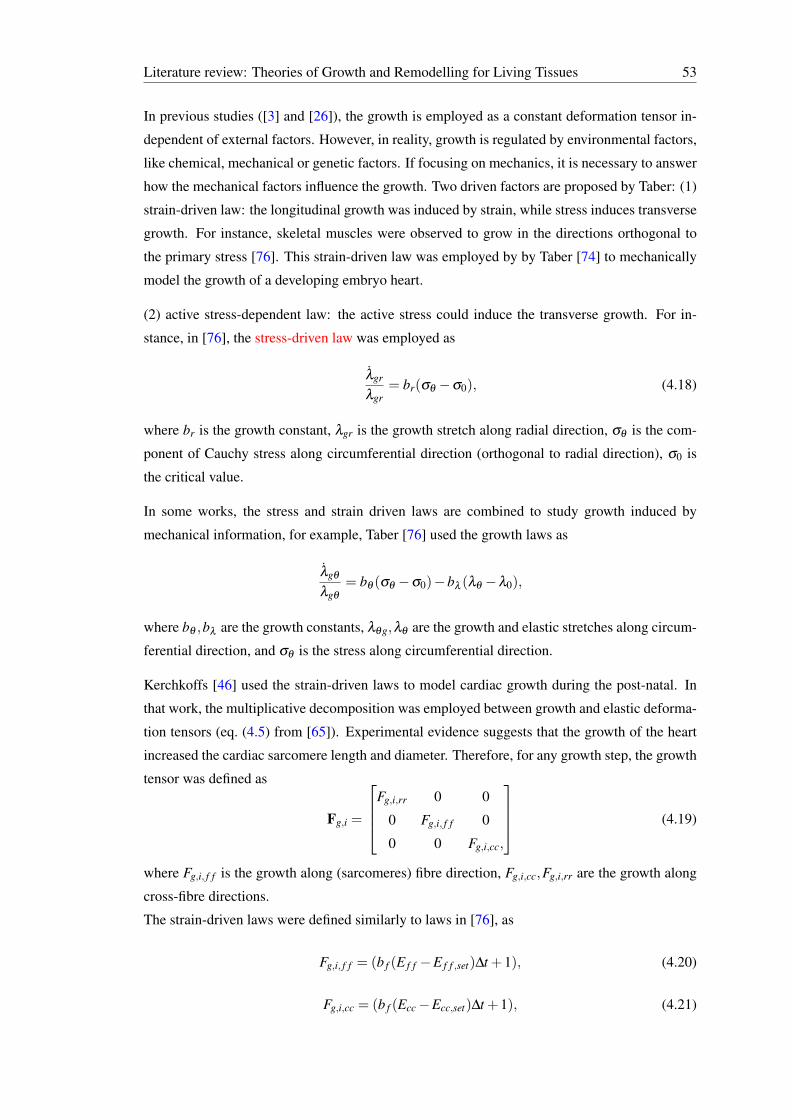
Literature review: Theories of Growth and Remodelling for Living Tissues 53
In previous studies ([3] and [26]), the growth is employed as a constant deformation tensor in-
dependent of external factors. However, in reality, growth is regulated by environmental factors,
like chemical, mechanical or genetic factors. If focusing on mechanics, it is necessary to answer
how the mechanical factors influence the growth. Two driven factors are proposed by Taber: (1)
strain-driven law: the longitudinal growth was induced by strain, while stress induces transverse
growth. For instance, skeletal muscles were observed to grow in the directions orthogonal to
the primary stress [76]. This strain-driven law was employed by by Taber [74] to mechanically
model the growth of a developing embryo heart.
(2) active stress-dependent law: the active stress could induce the transverse growth. For in-
stance, in [76], the stress-driven law was employed as
λgr
λgr= br(σθ −σ0), (4.18)
where br is the growth constant, λgr is the growth stretch along radial direction, σθ is the com-
ponent of Cauchy stress along circumferential direction (orthogonal to radial direction), σ0 is
the critical value.
In some works, the stress and strain driven laws are combined to study growth induced by
mechanical information, for example, Taber [76] used the growth laws as
λgθ
λgθ
= bθ (σθ −σ0)−bλ (λθ −λ0),
where bθ ,bλ are the growth constants, λθg,λθ are the growth and elastic stretches along circum-
ferential direction, and σθ is the stress along circumferential direction.
Kerchkoffs [46] used the strain-driven laws to model cardiac growth during the post-natal. In
that work, the multiplicative decomposition was employed between growth and elastic deforma-
tion tensors (eq. (4.5) from [65]). Experimental evidence suggests that the growth of the heart
increased the cardiac sarcomere length and diameter. Therefore, for any growth step, the growth
tensor was defined as
Fg,i =
Fg,i,rr 0 0
0 Fg,i, f f 0
0 0 Fg,i,cc,
(4.19)
where Fg,i, f f is the growth along (sarcomeres) fibre direction, Fg,i,cc,Fg,i,rr are the growth along
cross-fibre directions.
The strain-driven laws were defined similarly to laws in [76], as
Fg,i, f f = (b f (E f f −E f f ,set)∆t +1), (4.20)
Fg,i,cc = (b f (Ecc−Ecc,set)∆t +1), (4.21)
Literature review: Theories of Growth and Remodelling for Living Tissues 54
Fg,i,rr = Fg,i,cc, (4.22)
where Eii is the component of Eulerian strain tensor, and Eii,set is the threshold strain.
Then, the cumulative growth could be obtained as
Fng =
n
∏i=1
Fg,i. (4.23)
For the LV, the mechanical factors (such as strain) could be solved after setting boundary con-
ditions and material properties for the heart tissues in the FE method. Then, the local growth
would be induced following growth laws. After the geometric information of the LV is up-
dated by the growth, the mechanical information would be resolved and induce new growth. By
repeating this process, the long-term growth could be simulated.
However, one defect of the previous growth laws is that they might allow the ‘unbounded’
growth. For instance, in eq. (4.20), if the magnitude of fibre strain (E f f ) is significantly large,
it will induce the ‘large’ growth step. However, this is almost impossible in real living organs.
In [47], the growth laws are modified to exclude the ‘unbounded’ growth, as
Fg,i, f f =
k f ff f f ,max∆tgrowth
1+exp(− f f (sl−sl,50))+1, sl > 0
− f f f ,max∆tgrowth1+exp( f f (sl+sl,50))
+1, sl < 0,(4.24)
Fg,i,cc =
√kcc
fcc,max∆tgrowth1+exp(−c f (st−st,50))
+1, sl > 0√− f f f ,max∆tgrowth
1+exp(c f (st+st,50))+1, sl < 0,
(4.25)
where f f ,c f are growth constants, and si is the growth stimulus defined as
sl = max(E f f )−E f f ,set , sc = min(Ecc,max)−Ecc,set . (4.26)
Referring to eq. (4.25), the growth rate is actually bounded with upper limit value. For instance,
recalling eq. (4.25),
limsl=∞
Fg,i, f f = k f f f f f ,max∆tgrowth +1.
By applying this growth law, the heart growth was studied under pressure and volumetric over-
loads.
In [25], different growth laws were employed to study pathological and physiological growth
processes in the heart: it is assumed the driven factors are different for wall-thickening (stress-
driven) and ventricular dilation (strain-driven).
Literature review: Theories of Growth and Remodelling for Living Tissues 55
The adaptation in an athlete’s heart gives the increased heart pressure and volume. The stress-
driven growth law for the heart is given as
Fg = υgI, (4.27)
where υg is the growth multiplier which is determined by
υg = kg(υg) ·φ g(Me
)
kg = 1
τ( τmax−τg
τmax−1 )γ
φ g = tr(Me)−Me crit,(4.28)
where τ,γ are the growth constants, Me is the the Mandel stress (Me = CePe) and Me crit is the
criteria value.
This growth law induced isotropic cardiomyocyte growth, which increased the volume and wall
thickness of the LV.
The experimental observations suggest a transversely-isotropic growth during cardiac dilation.
The strain-driven growth law was defined as
Fg = I+(υg−1)f0⊗ f0, (4.29)
where f0 is the unit vector along the (sarcomere) fibre direction in the (fixed) reference configu-
ration. φ g is the growth multiplier which is determined by
υg = kg(υg) ·φ g(Fe
)
kg = 1
τ( τmax−τg
τmax−1 )γ
φ g = tr(Me)−Me crit ,(4.30)
where τ,γ are the growth constants.
This growth law induced transversely-isotropic growth which increased the volume of the LV
with constant wall thickness.
The experimental observations also suggest a transmural growth of heart muscle under pressure
overload. The stress-driven growth law was defined as
Fg = I+(υg−1)s0⊗ s0, (4.31)
where s0 is the unit vector orthotropic to the (sarcomere) fibre direction in the (fixed) reference
configuration, φ g is the growth multiplier which is determined by
υg = kg(υg) ·φ g(Me
)
kg = 1
τ( τmax−τg
τmax−1 )γ
φ g = tr(Me)−Me crit(4.32)
where τ,γ are the growth constants.
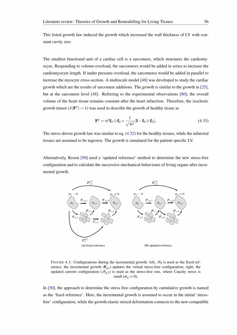
Literature review: Theories of Growth and Remodelling for Living Tissues 56
This listed growth law induced the growth which increased the wall thickness of LV with con-
stant cavity size.
The smallest functional unit of a cardiac cell is a sarcomere, which structures the cardiomy-
ocyte. Responding to volume-overload, the sarcomeres would be added in series to increase the
cardiomyocyte length. If under pressure-overload, the sarcomeres would be added in parallel to
increase the myocyte cross-section. A multiscale model [48] was developed to study the cardiac
growth which are the results of sarcomere additions. The growth is similar to the growth in [25],
but at the sarcomere level [48]. Referring to the experimental observations [80], the overall
volume of the heart tissue remains constant after the heart infarction. Therefore, the isochoric
growth tensor (J(Fg) = 1) was used to describe the growth of healthy tissue as
Fg = υgf0⊗ f0 +
1√υg
(I− f0⊗ f0), (4.33)
The stress-driven growth law was similar to eq. (4.32) for the healthy tissues, while the infarcted
tissues are assumed to be ingrown. The growth is simulated for the patient-specific LV.
Alternatively, Kroon [50] used a ‘updated reference’ method to determine the new stress-free
configuration and to calculate the successive mechanical behaviours of living organs after incre-
mental growth.
FIGURE 4.1: Configurations during the incremental growth: left, B0 is used as the fixed ref-erence, the incremental growth (Fg,i) updates the virtual stress-free configuration; right, theupdated current configuration (Bg,2) is used as the stress-free one, where Cauchy stress is
small (σg ≈ 0).
In [50], the approach to determine the stress free configuration by cumulative growth is named
as the ‘fixed reference’. Here, the incremental growth is assumed to occur in the initial ‘stress-
free’ configuration, while the growth-elastic mixed deformation connects to the new compatible
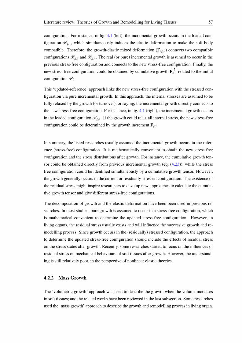
Literature review: Theories of Growth and Remodelling for Living Tissues 57
configuration. For instance, in fig. 4.1 (left), the incremental growth occurs in the loaded con-
figuration Bg,1, which simultaneously induces the elastic deformation to make the soft body
compatible. Therefore, the growth-elastic mixed deformation (Feg,2) connects two compatible
configurations Bg,1 and Bg,2. The real (or pure) incremental growth is assumed to occur in the
previous stress-free configuration and connects to the new stress-free configuration. Finally, the
new stress-free configuration could be obtained by cumulative growth F(2)n related to the initial
configuration B0.
This ‘updated-reference’ approach links the new stress-free configuration with the stressed con-
figuration via pure incremental growth. In this approach, the internal stresses are assumed to be
fully relaxed by the growth (or turnover), or saying, the incremental growth directly connects to
the new stress-free configuration. For instance, in fig. 4.1 (right), the incremental growth occurs
in the loaded configuration Bg,1. If the growth could relax all internal stress, the new stress-free
configuration could be determined by the growth increment Fg,2.
In summary, the listed researches usually assumed the incremental growth occurs in the refer-
ence (stress-free) configuration. It is mathematically convenient to obtain the new stress free
configuration and the stress distributions after growth. For instance, the cumulative growth ten-
sor could be obtained directly from previous incremental growth (eq. (4.23)), while the stress
free configuration could be identified simultaneously by a cumulative growth tensor. However,
the growth generally occurs in the current or residually-stressed configuration. The existence of
the residual stress might inspire researchers to develop new approaches to calculate the cumula-
tive growth tensor and give different stress-free configurations.
The decomposition of growth and the elastic deformation have been been used in previous re-
searches. In most studies, pure growth is assumed to occur in a stress-free configuration, which
is mathematical convenient to determine the updated stress-free configuration. However, in
living organs, the residual stress usually exists and will influence the successive growth and re-
modelling process. Since growth occurs in the (residually) stressed configuration, the approach
to determine the updated stress-free configuration should include the effects of residual stress
on the stress states after growth. Recently, some researches started to focus on the influences of
residual stress on mechanical behaviours of soft tissues after growth. However, the understand-
ing is still relatively poor, in the perspective of nonlinear elastic theories.
4.2.2 Mass Growth
The ‘volumetric growth’ approach was used to describe the growth when the volume increases
in soft tissues; and the related works have been reviewed in the last subsection. Some researches
used the ‘mass growth’ approach to describe the growth and remodelling process in living organ.
Literature review: Theories of Growth and Remodelling for Living Tissues 58
Baek [4] used the ‘constrained mixture model’ to study the growth of the aneurysms, which
model was initially developed by Humphrey [44]. The living organs are usually composed
of different constituents which continuously turnover during the life cycle. For an individual
constituent, the material or micro-structures are also turning over. For instance, the arteries
are composited by three key materials: smooth muscle, collagen and elastin; and the collagen
is continuously deposited and removed by fibroblast cells. Referring to nonlinear deformation
theories, the elastic states should be obtained by calculating the elastic deformation of arteries,
referring to the reference configurations of each constituent during turnover.
In the constrained mixture model, the reference (natural) configurations are different for old and
new material even for the same constituents. In [4], it is only turnover (growth and remodelling)
of collagen fibres in arteries is considered and the turnovers of elastin and muscle are ignored.
The newly-produced collagen (kth constituent of arteries) could be assembled into the loaded
configuration (Kτ ) of artery from its own stress-free configuration K kn (τ) at time t. If the
prestretch of new collagen was defined as a constant Gk(τ), the total elastic deformation here is
Fkn(τ)(t) = F(t)F−1(τ)Gk(τ), (4.34)
where F(t), F(τ) are the deformation tensors connected with subsequent configurations at time
t and τ from a universal reference configuration.
The total mass for individual constituent k was changed due to the local production and removal
of material, as
Mk(t) = Mk(0)Qk(t)+∫ t
mk(τ)qk(t− τ)dτ, (4.35)
where Qk(t) and qk(t) are the survival rates of constituents, mk is the rate of production, Mk is
the initial mass for constituent k. It is assumed that the density is constant for each individual
constituent, which means the mass changes of the constituents are proportional to the volumetric
changes.
The overall strain energy per unit volume could be obtained by
wk(t) =Mk(0)
ρk Qk(t)W k(Ft)+∫ t mk(τ)
ρk q(t− τ)W k(Fkn(τ))dτ. (4.36)
Then, the total strain energy per reference volume could be expressed
W (t) = ∑k
wk(t). (4.37)
Then, Cauchy stress could be obtained from the SEF related with time-dependent mass fractions
of the constituents. After solving the stress states for the boundary value problem with the helps
Literature review: Theories of Growth and Remodelling for Living Tissues 59
of the SEF (eq. 4.37), the collagen production could be obtain via a stress-driven G&R as
mk(t) = M(t)(Kg(σk(t)−1)+mk
h), (4.38)
where Kg is the growth parameter, mkh is the homeostatic value of mass for constituent k, M(t) is
the total mass at time t.
In [4], this approach was employed to study a developing aneurysm, in which the changed con-
stituent is collagen only.
As mentioned, the artery wall is composed of three key constituents: smooth muscle, collagen
and elastin. In [2], the constrained mixture model is used to analysis the growth and remod-
elling in an artery wall, while G&R processes occurred in all the key constituents. For elastin,
the experimental observations [11] suggests the turnovers of elastic are negligible. Then, the
additional stretch λ is assumed as 1 after turnover (no growth or remodelling). For collagen,
the stress-driven turning over is similar to that in [4] (eq. (4.38)). For smooth muscle, the used
growth laws indicates 1) the stress-driven growth of muscle along the radial direction, and 2) the
circumferential growth is induced by both strain and stress factors. By assembling the growth
laws into the SEF of an artery wall (eq. (4.37)), the SEF is obtained to describe the mechanical
behaviours of the artery under the framework of constrained mixture growth approach. In [2],
the stress state could be obtained to solve the boundary problems for a thick-wall artery tube
model. Coupling with the constrained mixture growth for artery constituents, the growth and
remodelling process is simulated for artery.
In previous researches from the Humphrey group ([4], [2]), the loads on living organs were
used as static and constant forces applied on the inner surface of the artery wall. Actually, the
loading and boundary conditions are dynamic and more complex than the constant loads, which
are induced by the interactions between the fluid (blood) and solid (artery walls) during life
cycle. By coupling the constrained mixture model with the fluid-solid interaction model, the
fluid-solid-growth is developed to study the cardiovascular growth and remodelling during the
cardiac cycle.
Applying the traction and stress continuity conditions at the fluid-solid interface, stress equi-
librium equations are solved for both the fluid and solid domains. Then, combined with the
constrained mixture model, the growth and remodelling process could be computed for the car-
diovascular vessel under fluid-solid-interaction conditions.
Most previous researches used the constrained mixture model, in which the studied cases are
relatively too simple in some sense: for example, using the thick-wall tube model describing
the mechanical behaviors of artery. However, from that clinical view, the problems are more
Literature review: Theories of Growth and Remodelling for Living Tissues 60
complex and challenging, which includes the hypodynamic or irregular geometry of the heart
and the boundary conditions. Valentin [84] implemented the constrained mixture model into a
FE model to simulate the growth and remodelling of an artery with a multilayer structure.
The evolution of the mechanical behaviours and growth in different artery layers were simu-
lated, which is a more-general tool to analyze the complex boundary problem associated with
patient-specific geometries ([4, 43]).
Watton [92, 94] also employed different configurations to describe the growth and remodelling
in different constituents of living organs. In [94], the artery wall is assumed to be composed of
two constituents: extracellular matrix (ECM) and collagen. For ECM, the degradation of elastin
is fitted from experimental data.
For collagen: 1) all collagen fibres will be deposited into the recruitment configuration with
different recruitment stretches. Recruitment stretch, firstly introduced in [93], is to describe the
onset stretch of recruitment of fibres to bear loads. 2) the strain-driven growth law of collagen
could be also obtained from experimental data as
dmC
dt= (ξ1mC +ξ2|
dmE
dt|)(EC−EC
AT ) (4.39)
where ξi is the remodelling constant.
By coupling the remodelling-growth laws and the SEF, the evolution of remodelling and the
mechanical behaviours are obtained by solving the boundary problem for the thick-wall artery
model. However, to author, the remodelling-growth framework is only suitable for limited cases,
and is not satisfactory for solving general problems. For instance, it is assumed all collagen fi-
bres are deposited in the fixed recruitment configuration. However, the fibres, deposited by
fibroblast cells, are usually produced in the current configuration, while cells don’t ‘know’ the
recruitment configuration. Besides, from the mechanical perspective, the SEF used in [94] is
defined for per volume for artery tissues (eq. (4.40)). Then, the sum of weights from the con-
stituents (collagen and ECM) should be one, which guarantees the SEF for tissues is always
defined for unit volume as
mC +mE ≡ 1.
However, the volumetric fractions of constituents are independently regulated by their own
remodelling-growth laws. If mC + mE 6= 1, the SEF might not give the proper stress-strain
relation. Moreover, other limitations are also included in that framework.
The different formulations of artery wall were experimentally observed ([69]): for an individ-
ual constituent, the material density remains constant during life, which is named as ‘constant
Literature review: Theories of Growth and Remodelling for Living Tissues 61
individual density’ (CID). If the material density is changing, it is called ‘adaptive individual
density’ (AID). Eriksson [16] modified the remodelling-growth laws (eq. 4.39) and the SEF
with the material density factors to describe the mechanical behaviours of an artery and applied
them in the FE method. The SEF is modified as
Ψ = ρeΨE + ρCΨ
C, (4.40)
where ρe, ρC are density factors for elastin and collagen.
If the density ρξ is constant for constituent ξ (CID), the density factor at time τ is expressed as
ρξ (τ) =ρξ (τ)
ρξ (τ0)=
vξ (τ)
v(τ)(4.41)
where vξ (τ) is the volumetric factor of constituent ξ , v(τ) is the volumetric fraction of tissue.
If the density ρξ is adaptive for constituent ξ (AID), the density factor at time τ is expressed as
ρξ (τ) =ρξ (τ)
ρξ (τ0)= ρξ 0(τ)
vξ (τ)
v(τ), (4.42)
where ρξ (τ) is the individual (unnormalized) density.
Combining with the growth laws of collagen and elastin, the SEF is obtained for artery tissues
during the remodelling-growth process. This framework is assembled into the FE method to
simulate the evolution of the artery structure during the life cycle with different growth patterns
(CID or AID).
Volokh [86] used a phenomenological theory of tissue growth and develop a toy-like model to
describe tumor growth. In [86], the growth is explained as: considering a regular initial tissue,
the new tissue elementary components (cells, molecules) are supplied, which is seen as a result
of injection. And it could be constructed physically into a model of tissue growth. In this model,
the stress-strain relation is redefined as
P = F(∂W/∂E− (ρ−ρ0)η), (4.43)
where W is the SEF for non-growing tissue, P is the first Piola-Kirchohoff stress, η is the grown
moduli tensor, which is related to the tissue growth and independent from mechanical factors.
This growth law is obviously different from other researches ([2], [4]). In [86], the tumor is
simulated as a multi-layer spheroid. The simulation of tumor growth agreed with in vitro exper-
imental observation.
Literature review: Theories of Growth and Remodelling for Living Tissues 62
4.3 Summary and Theoretical Gaps
Understanding of G&R is obviously improved in previous researches. The fibre remodelling
is simulated with different regulators. It is analytically demonstrated that the fibre structure is
optimized to bear the external loading. However, the limitations are also obvious in those works.
To this author, the most important problem is: in real living tissues, the fibre turnover usually
includes two key processes: the fibre deposition and re-orientation. In most of researches, the
remodelling is decoupled from volumetric growth. Then, if the fibre is deposited in the current
configuration, the push-back method is employed to obtain the fibre structure in the stress free
configuration, i.e.
f′0 = F−1e f,
where f′0, f are fibre vectors in stress free and loaded configurations.
However, if the tissues experience both turnover of the fibres and volumetric growth, the method
is more complex to obtain the fibre structure in the stress-free configuration. In general, if the
fibre rotation and volumetric growth occur in the current configuration, the fibre structure should
be carried into the grown configuration according to
f′ = Gf,
where f′, f are the fibre vectors in loaded and grown configurations.
After the previous step, assuming the updated stress-free configuration could be obtained by
fully releasing the residual stress, the fibre vector is updated as
f′0 = F−1τ f,
where f′0 is the fibre vector in the updated stress-free configuration, and Fτ is the elastic defor-
mation tensor connecting the updated stress-free and residually-stress configurations.
The coupled remodelling and volumetric model for the fibre structure is really needed fordetermining the evolution of the fibre structure and the material properties.
Another theoretical gap is: For the volumetric growth, currently, it is assumed that the growth
occurs in the stress-free or unloaded configuration, which is computationally convenient. How-
ever, in real organs, the stress is always existing which condition requires to assuming the growth
occurs in the stressed configuration. Then, the material properties will obviously differ from the
tissue with growth in stress-free configuration. In some works, the importance of investigating
the growth in stressed configuration is addressed. However, in those researches, the framework
is not given to properly compute the growth. It is important for investigating the influence of
Literature review: Theories of Growth and Remodelling for Living Tissues 63
growth on the mechanical behaviours, which is fundamental for really understanding the mech-
anisms of G&R in living organs.
From a general perspective mechanics to investigate the G&R process in living tissues, the ques-
tions are: How does the residual stress influence the fibre remodelling and the material properties
of entire organs? How to determine the combined effects of growth (in the stressed configura-
tion) and remodelling on the fibre structure? How to develop a framework for investigating
G&R processes occurring in the stressed configuration?
Chapter 5
Residual Stress from Multi-cutOpening Angle Models of the LeftVentricle
5.1 Introduction
Living tissues in the heart continuously interact with the external bio-environment, reshape and
rearrange their constituents under chemical, mechanical or genetic stimuli during their life cy-
cles. In the mature period, these processes remain in a homeostatic state. However, heart dis-
eases will disrupt the balance, and the tissues will grow and remodel in response to an insult.
Physiologically, exercise may also induce healthy and reversible growth and remodelling. An
important ingredient in evaluating the mechanics involved in the cardiovascular system is knowl-
edge of the solid mechanical properties of the soft tissues involved, including the components
of the heart (such as the left ventricle). A particular aspect is that the soft tissues possess resid-
ual stress in vivo, so that when the external loading is removed, residual stresses remain in the
material. However, residual stresses, which are generally considered to result from growth and
remodelling, are imprecisely characterized (experimentally) at present, and how best to include
the important effect of residual stress in cardiovascular applications therefore presents a mod-
elling challenge.
Over the last century [40], various hypotheses on the growth and remodelling response to me-
chanical loading have been put forward, with particular success in arteries. Traditionally, one of
the fundamental ideas is to assume the existence of a (stress-free) reference configuration [57],
which coincides with the unloaded configuration. In the present context, however, the unloaded
configuration is not stress free, but is residually stressed. The residual stress can be estimated
using the so-called opening angle method [8, 52], in which an opening angle indicative of the
64
Residual Stress from Multi-cut Opening Angle Models of the Left Ventricle 65
extent of the residual stress can be measured after a single radial cut of an unloaded arterial ring.
Using the opened configuration as the reference configuration, the residual stress of a cylindrical
artery model can be estimated[8, 77]. This methodology has been extended to multiple cuts by
Taber and Humphrey [78], and used in the two-layered arterial models by Holzapfel et al. [34].
Residual stress is important in modelling the mechanics of soft tissues for a number of reasons:
(a) in nonlinear elasticity theory the stress state in the reference configuration has a substantial
effect on the subsequent response to the loads, and omission of the residual stress leads to
significantly different total stress predictions [55], for example, the stress distribution in mice
heart is simulated under hear pressure [90]. The estimation of maximal principal stress increased
about 40% after introducing the residual stress; (b) in biological tissues, the residual stress is
a result of growth [54]; (c) while the detailed process of local growth is difficult to measure,
residual stress, on the other hand, may be estimated from experiments, as demonstrated by the
opening angle measurement. Thus, a properly estimated residual stress at particular time instants
could provide useful information about the growth history of living tissues.
However, work that includes residual stress in complex organs, such as the heart, remains rare.
A few existing models for the left ventricle that take account of residual stress are based on the
assumption that a simple radial cut can release all the residual stresses [90], but this assumption
is not supported by all experiments. For example, Omens et al. [59] showed that residual stress
in a mouse primary heart can be further released by a circumferential cut following the initial
radial cut, as illustrated in fig. 5.1. This implies that the single cut opening angle configuration
does not correspond to the stress-free configuration.
Inspired by the experiments [59], in this chapter, we develop multi-cut models in order to esti-
mate the residual stress distribution across the wall of an intact mature heart based on a simplified
heart model.
5.2 Methodology
For the material model of incompressible heart tissues, we use a reduced version of the invariant-
based constitutive law for the myocardium developed by Holzapfel and Ogden [35], subse-
quently referred to as the HO model, namely
Ψ = Ψm +Ψf, (5.1)
where
Ψm =a2bexp[b(I1−3)]−1, Ψf =
af
2bfexp[bf(I4−1)2]−1, (5.2)
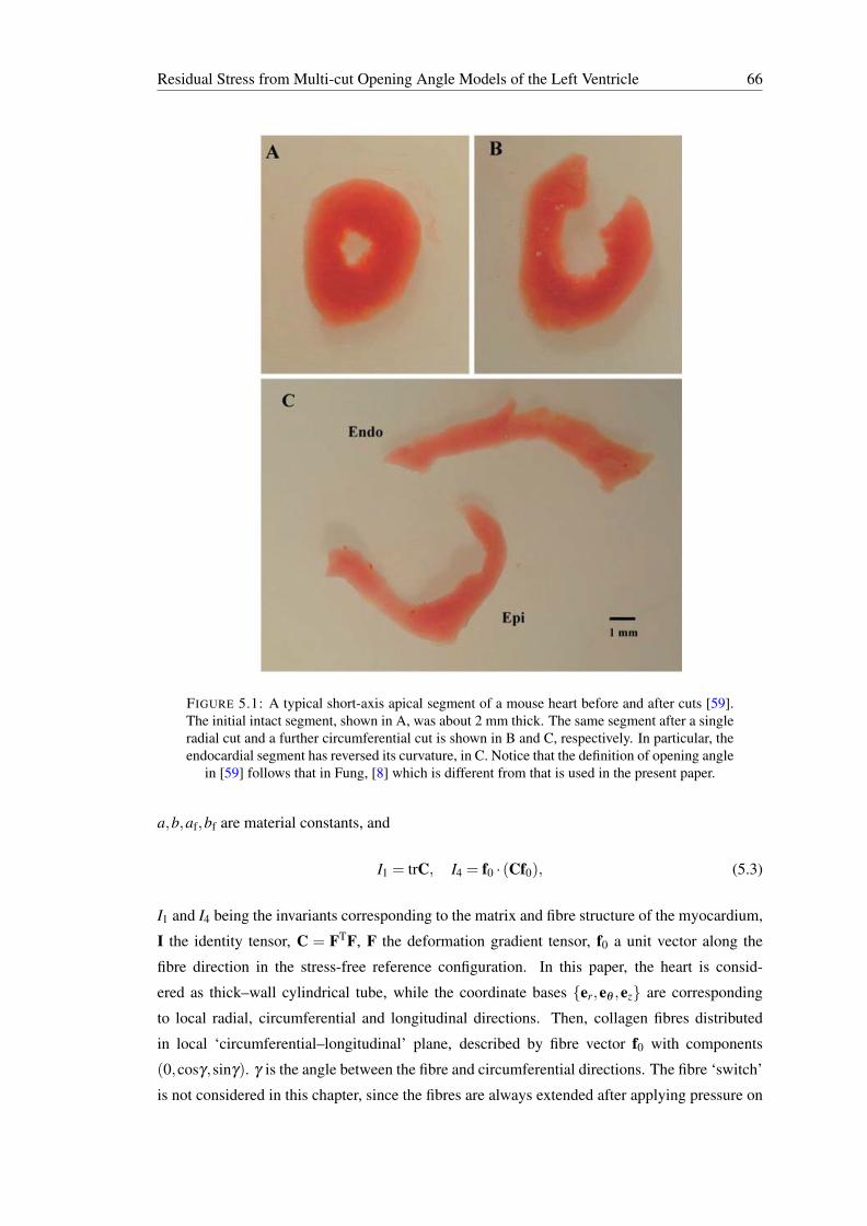
Residual Stress from Multi-cut Opening Angle Models of the Left Ventricle 66
FIGURE 5.1: A typical short-axis apical segment of a mouse heart before and after cuts [59].The initial intact segment, shown in A, was about 2 mm thick. The same segment after a singleradial cut and a further circumferential cut is shown in B and C, respectively. In particular, theendocardial segment has reversed its curvature, in C. Notice that the definition of opening angle
in [59] follows that in Fung, [8] which is different from that is used in the present paper.
a,b,af,bf are material constants, and
I1 = trC, I4 = f0 · (Cf0), (5.3)
I1 and I4 being the invariants corresponding to the matrix and fibre structure of the myocardium,
I the identity tensor, C = FTF, F the deformation gradient tensor, f0 a unit vector along the
fibre direction in the stress-free reference configuration. In this paper, the heart is consid-
ered as thick–wall cylindrical tube, while the coordinate bases er,eθ ,ez are corresponding
to local radial, circumferential and longitudinal directions. Then, collagen fibres distributed
in local ‘circumferential–longitudinal’ plane, described by fibre vector f0 with components
(0,cosγ,sinγ). γ is the angle between the fibre and circumferential directions. The fibre ‘switch’
is not considered in this chapter, since the fibres are always extended after applying pressure on
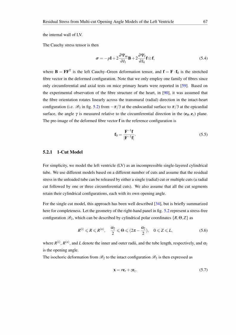
Residual Stress from Multi-cut Opening Angle Models of the Left Ventricle 67
the internal wall of LV.
The Cauchy stress tensor is then
σ =−pI+2∂Ψm
∂ I1B+2
∂Ψf
∂ I4f⊗ f, (5.4)
where B = FFT is the left Cauchy–Green deformation tensor, and f = F · f0 is the stretched
fibre vector in the deformed configuration. Note that we only employ one family of fibres since
only circumferential and axial tests on mice primary hearts were reported in [59]. Based on
the experimental observation of the fibre structure of the heart, in [90], it was assumed that
the fibre orientation rotates linearly across the transmural (radial) direction in the intact-heart
configuration (i.e. B3 in fig. 5.2) from −π/3 at the endocardial surface to π/3 at the epicardial
surface, the angle γ is measured relative to the circumferential direction in the (eθ ,ez) plane.
The pre-image of the deformed fibre vector f in the reference configuration is
f0 =F−1f|F−1f| . (5.5)
5.2.1 1-Cut Model
For simplicity, we model the left ventricle (LV) as an incompressible single-layered cylindrical
tube. We use different models based on a different number of cuts and assume that the residual
stress in the unloaded tube can be released by either a single (radial) cut or multiple cuts (a radial
cut followed by one or three circumferential cuts). We also assume that all the cut segments
retain their cylindrical configurations, each with its own opening angle.
For the single cut model, this approach has been well described [34], but is briefly summarized
here for completeness. Let the geometry of the right-hand panel in fig. 5.2 represent a stress-free
configuration B2, which can be described by cylindrical polar coordinates R,Θ,Z as
R(i) 6 R6 R(o),α2
26Θ6 (2π− α2
2), 06 Z 6 L, (5.6)
where R(i), R(o), and L denote the inner and outer radii, and the tube length, respectively, and α2
is the opening angle.
The isochoric deformation from B2 to the intact configuration B3 is then expressed as
x = rer + zez. (5.7)
Residual Stress from Multi-cut Opening Angle Models of the Left Ventricle 68
Material incompressibility gives
r =
√√√√R2−R(i)2
kλ(3)z
+ r(i)2, θ = k(Θ−α2/2), z = λ
(3)z Z, (5.8)
where r(i) is the inner radius in the configuration B3, λ(3)z = l/L is the constant axial stretch,
where l is the cylinder length in B3, while k = 2π/(2π−α2) is a measure of the opening angle
in B2. The outer radius in B3 is
r(o) =
√√√√R(o)2−R(i)2
kλ(3)z
+ r(i)2. (5.9)
angle in B2. The outer radius in B3 is
r(o) =
√R(o)2 −R(i)2
kλ(3)z
+ r(i)2. (8)
(a) (b)
B3 B2
F(3)α2
Figure 2: 1-cut model: cylindrical model of the LV after a single radial cut of the intact
unloaded configuration B3 into a stress-free sector B2.
The corresponding deformation gradient (from B2 to the intact ring configuration B3),
denoted F(3), is given by
F(3) = λ(3)1 er ⊗ ER + λ
(3)2 eθ ⊗ EΘ + λ(3)
z ez ⊗ EZ , (9)
where
λ(3)1 =
R
rkλ(3)z
, λ(3)2 =
kr
R(10)
and ER,EΘ,EZ are cylindrical polar axes in B2. It follows that the invariants I1 and I4
(with the superscript (3) omitted temporarily for simplicity) are given by
I1 = λ21 + λ2
2 + λ2z, I4 = λ2
2 cos2 γ + λ2z sin2 γ, (11)
where the components of f0 and f are (0, cos γ, sin γ)T and (0, λ2 cos γ, λz sin γ)T, respectively,82
and γ is the angle defining the fibre orientation with respect to the circumferential direction83
in B2.84
6
FIGURE 5.2: 1-cut model: cylindrical model of the LV after a single radial cut of the intactunloaded configuration B3 into a stress-free sector B2.
The corresponding deformation gradient (from B2 to the intact ring configuration B3), denoted
F(3), is given by
F(3) = λ(3)1 er⊗ER +λ
(3)2 eθ ⊗EΘ +λ
(3)z ez⊗EZ, (5.10)
where
λ(3)1 =
R
rkλ(3)z
, λ(3)2 =
krR
(5.11)
the superscript (i = 1,2,3) indicates the variable related to the target configuration Bi and
ER,EΘ,EZ are cylindrical polar axes in B2.
It follows that the invariants I1 and I4 (with the superscript (3) omitted temporarily for simplicity)
are given by
I1 = λ21 +λ
22 +λ
2z , I4 = λ
22 cos2
γ +λ2z sin2
γ, (5.12)
where the components of f0 and f are (0,cosγ,sinγ)T and (0,λ2 cosγ,λz sinγ)T, respectively,
and γ is the angle defining the fibre orientation with respect to the circumferential direction in
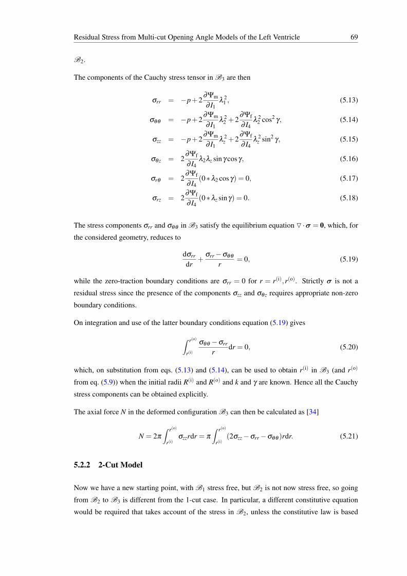
Residual Stress from Multi-cut Opening Angle Models of the Left Ventricle 69
B2.
The components of the Cauchy stress tensor in B3 are then
σrr = −p+2∂Ψm
∂ I1λ
21 , (5.13)
σθθ = −p+2∂Ψm
∂ I1λ
22 +2
∂Ψf
∂ I4λ
22 cos2
γ, (5.14)
σzz = −p+2∂Ψm
∂ I1λ
2z +2
∂Ψf
∂ I4λ
2z sin2
γ, (5.15)
σθz = 2∂Ψf
∂ I4λ2λz sinγ cosγ, (5.16)
σrθ = 2∂Ψf
∂ I4(0∗λ2 cosγ) = 0, (5.17)
σrz = 2∂Ψf
∂ I4(0∗λz sinγ) = 0. (5.18)
The stress components σrr and σθθ in B3 satisfy the equilibrium equation O ·σ = 0, which, for
the considered geometry, reduces to
dσrr
dr+
σrr−σθθ
r= 0, (5.19)
while the zero-traction boundary conditions are σrr = 0 for r = r(i),r(o). Strictly σ is not a
residual stress since the presence of the components σzz and σθz requires appropriate non-zero
boundary conditions.
On integration and use of the latter boundary conditions equation (5.19) gives
∫ r(o)
r(i)
σθθ −σrr
rdr = 0, (5.20)
which, on substitution from eqs. (5.13) and (5.14), can be used to obtain r(i) in B3 (and r(o)
from eq. (5.9)) when the initial radii R(i) and R(o) and k and γ are known. Hence all the Cauchy
stress components can be obtained explicitly.
The axial force N in the deformed configuration B3 can then be calculated as [34]
N = 2π
∫ r(o)
r(i)σzzrdr = π
∫ r(o)
r(i)(2σzz−σrr−σθθ )rdr. (5.21)
5.2.2 2-Cut Model
Now we have a new starting point, with B1 stress free, but B2 is not now stress free, so going
from B2 to B3 is different from the 1-cut case. In particular, a different constitutive equation
would be required that takes account of the stress in B2, unless the constitutive law is based
Residual Stress from Multi-cut Opening Angle Models of the Left Ventricle 70
(a) (b) (c)
B3 B2 B1
F(3) F(2)
α2 α(2)1 α
(1)1
outerouter
innerinner
Figure 3: The 2-cut model: (a) cylindrical model of the LV as the intact ring in B3, (b) after
a radial cut to B2, and (c) followed by a circumferential cut to B1. Notice that the inner
segment in B1 has a negative curvature, as in [14]. The red curve, at the mid-wall radius
R = (R(i) +R(o))/2 in (b), separates the inner and outer sectors which become the separate
inner and outer sectors in B1 after the circumferential cut.
2-Cut Model95
In the 2-cut model, following a radial cut, a circumferential cut is performed around the
mid-wall in B2 at radius R = (R(i) +R(o))/2. It is assumed now that residual stress remains
after the radial cut but is removed after the circumferential cut and that no axial deformation
is associated with the second cut. The resulting stress-free configuration B1 is depicted in
Fig. 3. We note, in particular, that following the circumferential cut the inner segment has a
negative curvature. The geometry in B1 is described in terms of cylindrical polar coordinates
R,Θ, Z, with subscripts 1 and 2 corresponding to the inner and outer sectors, respectively.
Thus,
R(i)1 6 R1 6 R
(o)1 , −(π − α
(1)1
2) 6 Θ1 6 π − α
(1)1
2, 0 6 Z1 6 L, (19)
R(i)2 6 R2 6 R
(o)2 ,
α(2)1
26 Θ2 6 2π − α
(2)1
2, 0 6 Z2 6 L, (20)
where R(i)j , R
(o)j , α
(j)1 , j = 1, 2, and L denote the inner and outer radii, the opening angles,96
and the tube length in B1. In B2, R(i)1 and R
(i)2 both become R, while R
(o)1 and R
(o)2 translate97
8
FIGURE 5.3: The 2-cut model: (a) cylindrical model of the LV as the intact ring in B3, (b)after a radial cut to B2, and (c) followed by a circumferential cut to B1. Notice that the innersegment in B1 has a negative curvature, as in [59]. The red curve, at the mid-wall radiusR = (R(i) +R(o))/2 in (b), separates the inner and outer sectors which become the separate
inner and outer sectors in B1 after the circumferential cut.
on B1. In the 2-cut model, following a radial cut, a circumferential cut is performed around
the mid-wall in B2 at radius R = (R(i)+R(o))/2. It is assumed now that residual stress remains
after the radial cut but is removed after the circumferential cut and that no axial deformation is
associated with the second cut. The resulting stress-free configuration B1 is depicted in fig. 5.3.
We note, in particular, that following the circumferential cut the inner segment has a negative
curvature. The geometry in B1 is described in terms of cylindrical polar coordinates R,Θ,Z,with subscripts 1 and 2 corresponding to the inner and outer sectors, respectively. Thus,
R(i)1 6 R1 6 R(o)
1 , −(π− α(1)12
)6Θ1 6 π− α(1)12
, 06 Z1 6 L, (5.22)
R(i)2 6 R2 6 R(o)
2 ,α(2)126Θ2 6 2π− α
(2)12
, 06 Z2 6 L, (5.23)
where R(i)j , R(o)
j , α( j)1 , j = 1,2, and L denote the inner and outer radii, the opening angles, and
the tube length in B1. In B2, R(i)1 and R(i)
2 both become R, while R(o)1 and R(o)
2 translate to R(i)
and R(o), respectively, the opening angle is α2 and the axial length l.
For each segment, the isochoric deformation from B1 to B2 can be written as
X = RER +ZEZ, (5.24)
with
R =
√√√√R(i)1
2−R2
1
k1λ(21)z
+ R2, Θ = π− k1Θ1, Z = λ(21)z Z1 (5.25)
R =
√√√√R22−R(i)
22
k2λ(22)z
+ R2, Θ = k2(Θ2−π)+π, Z = λ(22)z Z2 (5.26)
for the inner and outer sectors, respectively, where λ(2 j)z is taken to be 1 for both segments and
k j = (2π−α2)/(2π−α( j)1 ), j = 1,2. Note that the negative curvature of the inner segment in B1
Residual Stress from Multi-cut Opening Angle Models of the Left Ventricle 71
depicted in fig. 5.3 is captured by the expression for R in (5.25), and that structural compatibility
is ensured since the two expressions for R match at R.
As indicated in fig. 5.3 the deformation gradient from B1 to B2 is denoted F(2), which is short-
hand notation for the two separate deformation gradients from the two sectors in B1 to B2.
These are denoted F(2 j), j = 1,2, and given by
F(2 j) = λ(2 j)1 er⊗ER +λ
(2 j)2 eθ ⊗EΘ +λ
(2 j)z ez⊗EZ, (5.27)
where
λ(2 j)1 =
R j
k jRλ(2 j)z
, λ(2 j)2 =
k jRR j
, λ(2 j)z = 1.14, j = 1,2. (5.28)
Similarly to the 1-cut model, and with the same notation for the stress components, the equilib-
rium equation in B2 yields
dσrr
dr+
σrr−σθθ
r= 0,
∫ R(o)
R(i)
σθθ −σrr
rdr = 0. (5.29)
Equation (5.29)1 can be rearranged as
σθθ =ddr
(rσrr), (5.30)
from which it follows, on use of the zero-traction boundary conditions on R(i) and R(o), that
∫ R(o)
R(i)σθθ dr = 0, (5.31)
i.e. the mean value of σθθ is zero.
It’s assumed that is there is no bending moment on the faces Θ = α2/2 and Θ = 2π−α2/2 in
B2, which yields∫ R(o)
R(i)σθθ rdr = 0. (5.32)
Substitution of σθθ from (5.30) into this equation followed by integration by parts and a further
application of the zero-traction boundary conditions leads to
∫ R(o)
R(i)σrrrdr = 0. (5.33)
Equations (5.29)2, (5.31) and (5.33) are solved with equations (5.25) and (5.26) to obtain the
radius R(i), and the angle α2 of the segment in B2. In B2, the radial traction σrr is continuous
across interface r, since the deformation gradient, Lagrangian multiplier p and the other stress
Residual Stress from Multi-cut Opening Angle Models of the Left Ventricle 72
components are continuous. The continuity of hoop stress yields
(σθθ |r=r)+ = (σθθ |r=r)
−, (5.34)
where r are the radial positions of the interfaces (r = r(o)+r(i)2 ).
The stress continuity will help to exclude the redundant solutions of R(i) and the angle α2 from
equations (5.29)2 and (5.33).
Once R(i), R(o) and α2 are obtained, the 1-cut approach is used to estimate the residual stress of
the intact-ring configuration.
It’s worthy to emphasize that asymmetry in local fibre structure leads to the non-zero torsion
boundary condition in B2, which yields
∫ R(o)
R(i)σθzdr 6= 0.
However, actually, comparing with σrr or σθθ , the shear component at cross-section of the
tube is ignorably small. Then, the mechanical contributions of shear stress are assumed to be
ignorable to stress equilibrium and the shape changing of cylindrical geometry of heart tube.
And this assumption will also be mathematically applied in our 4-cut model later.
Essentially, this is equivalent to calculating the deformation gradient from B1 to B3 by mul-
tiplication as F(3)F(2), where F(3) is given by eq. (5.10) and F(2) is either F(21) or F(22) and
determined from eq. (5.27).
An expression for the axial load N is obtained from a formula similar to that in eq. (5.21).
It suggests that ’infinite cuts’ are efficient to release all residual stress in living organs, since
residual stress is induced by the complex (inhomogeneous) growth. Therefore, 4-cut model may
give better estimations for residual stress.
The mechanical behaviors of LV are calculated with the single fibre family. According to the
discussion about the effect of shear stress on the mechanical response of LV tube, it shows that
the geometric shape doesn’t change much by the shear stress. Therefore, the effects of shear
stress are really ignorable, while the values of shear stresses are really small.
The stress distributions in 1-cut configuration are obtained from both stress and deformation
continuity conditions. And it shows that stress continuity is almost equivalent with deformation
continuity in multiple-cut model.
The computation results explain experimental observation by Fung [23]. In the residually
stressed configuration of an artery, the subsequent radial cuts don’t introduce any more elas-
tic deformations. Moreover, no solid evidence supports that the 1-cut configuration is the stress
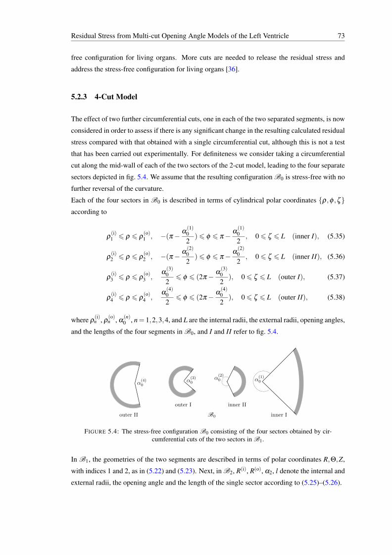
Residual Stress from Multi-cut Opening Angle Models of the Left Ventricle 73
free configuration for living organs. More cuts are needed to release the residual stress and
address the stress-free configuration for living organs [36].
5.2.3 4-Cut Model
The effect of two further circumferential cuts, one in each of the two separated segments, is now
considered in order to assess if there is any significant change in the resulting calculated residual
stress compared with that obtained with a single circumferential cut, although this is not a test
that has been carried out experimentally. For definiteness we consider taking a circumferential
cut along the mid-wall of each of the two sectors of the 2-cut model, leading to the four separate
sectors depicted in fig. 5.4. We assume that the resulting configuration B0 is stress-free with no
further reversal of the curvature.
Each of the four sectors in B0 is described in terms of cylindrical polar coordinates ρ,φ ,ζaccording to
ρ(i)1 6 ρ 6 ρ
(o)1 , −(π− α
(1)02
)6 φ 6 π− α(1)02
, 06 ζ 6 L (inner I), (5.35)
ρ(i)2 6 ρ 6 ρ
(o)2 , −(π− α
(2)02
)6 φ 6 π− α(2)02
, 06 ζ 6 L (inner II), (5.36)
ρ(i)3 6 ρ 6 ρ
(o)3 ,
α(3)026 φ 6 (2π− α
(3)02
), 06 ζ 6 L (outer I), (5.37)
ρ(i)4 6 ρ 6 ρ
(o)4 ,
α(4)026 φ 6 (2π− α
(4)02
), 06 ζ 6 L (outer II), (5.38)
where ρ(i)n , ρ
(o)n , α
(n)0 , n= 1,2,3,4, and L are the internal radii, the external radii, opening angles,
and the lengths of the four segments in B0, and I and II refer to fig. 5.4.
B0
α(4)0
α(3)0
α(2)0 α
(1)0
outer II
outer I inner II
inner I
Figure 4: The stress-free configuration B0 consisting of the four sectors obtained by circum-
ferential cuts of the two sectors in B1.
mation gradients from B1 to B2 which also have to be continuous, and the deformation137
gradient in B3 likewise has to be continuous. The consequences of these constraints now138
need to be evaluated.139
The deformations from the four sectors in B0 to the two sectors in B1 are described by
R1 =
√√√√ρ2 − ρ(i)1
2
k11λ(11)z
+ R21, Θ1 = k11φ, Z1 = λ(11)
z ζ, (inner I), (35)
R1 =
√√√√ρ2 − ρ(o)2
2
k12λ(12)z
+ R21, Θ1 = k12φ, Z1 = λ(12)
z ζ, (inner II), (36)
R2 =
√√√√ρ2 − ρ(o)3
2
k23λ(23)z
+ R22, Θ2 = k23(φ− π) + π, Z2 = λ(23)
z ζ, (outer I), (37)
R2 =
√√√√ρ2 − ρ(i)4
2
k24λ(24)z
+ R22, Θ2 = k24(φ− π) + π, Z2 = λ(24)
z ζ, (outer II), (38)
where
k1n = (2π − α(1)1 )/(2π − α(n)
0 ), n = 1, 2, k2n = (2π − α(2)1 )/(2π − α(n)
0 ), n = 3, 4,
λ(1n)1 =
R1
ρk1nλ(1n)z
, λ(1n)2 =
k1nρ
R1
, n = 1, 2,
12
FIGURE 5.4: The stress-free configuration B0 consisting of the four sectors obtained by cir-cumferential cuts of the two sectors in B1.
In B1, the geometries of the two segments are described in terms of polar coordinates R,Θ,Z,
with indices 1 and 2, as in (5.22) and (5.23). Next, in B2, R(i), R(o), α2, l denote the internal and
external radii, the opening angle and the length of the single sector according to (5.25)–(5.26).
Residual Stress from Multi-cut Opening Angle Models of the Left Ventricle 74
The deformations from the four sectors in B0 to the two sectors in B1 are described by
R1 =
√√√√ρ2−ρ(i)1
2
k11λ(11)z
+ R21, Θ1 = k11φ , Z1 = λ
(11)z ζ , (inner I), (5.39)
R1 =
√√√√ρ2−ρ(o)2
2
k12λ(12)z
+ R21, Θ1 = k12φ , Z1 = λ
(12)z ζ , (inner II), (5.40)
R2 =
√√√√ρ2−ρ(o)3
2
k23λ(23)z
+ R22, Θ2 = k23(φ −π)+π, Z2 = λ
(23)z ζ , (outer I), (5.41)
R2 =
√√√√ρ2−ρ(i)4
2
k24λ(24)z
+ R22, Θ2 = k24(φ −π)+π, Z2 = λ
(24)z ζ , (outer II), (5.42)
where
k1n = (2π−α(1)1 )/(2π−α
(n)0 ), n = 1,2, k2n = (2π−α
(2)1 )/(2π−α
(n)0 ), n = 3,4,
λ(1n)1 =
R1
ρk1nλ(1n)z
, λ(1n)2 =
k1nρ
R1, n = 1,2,
and
λ(2n)1 =
R2
ρk2nλ(2n)z
, λ(2n)2 =
k2nρ
R2, n = 3,4.
The deformation gradients from B0 in fig. 5.4 to B1 in fig. 5.3 are
F(1n) = λ(1n)1 ER⊗ eρ +λ
(1n)2 EΘ⊗ eφ +λ
(1n)z EZ⊗ eζ , n = 1,2, (5.43)
F(1n) = λ(2n)1 ER⊗ eρ +λ
(2n)2 EΘ⊗ eφ +λ
(2n)z EZ⊗ eζ , n = 3,4. (5.44)
In B1, the radial direction for each of the two segments yields
∫ R(o)j
R(i)j
σΘΘ−σRR
RdR = 0, j = 1,2. (5.45)
The radial traction σRR should be continuous across each interface R j, j = 1,2, and hence, since
the deformation gradient is continuous, p is continuous and the other stress components are also
continuous. The continuity of hoop stress yields
(σΘΘ|R=Rk)+ = (σΘΘ|R=Rk)
−, k = 1,2, (5.46)
where Rk are the radial positions of the interfaces (Rk =R(o)
j +R(i)j+1
2 , j = 1,2)
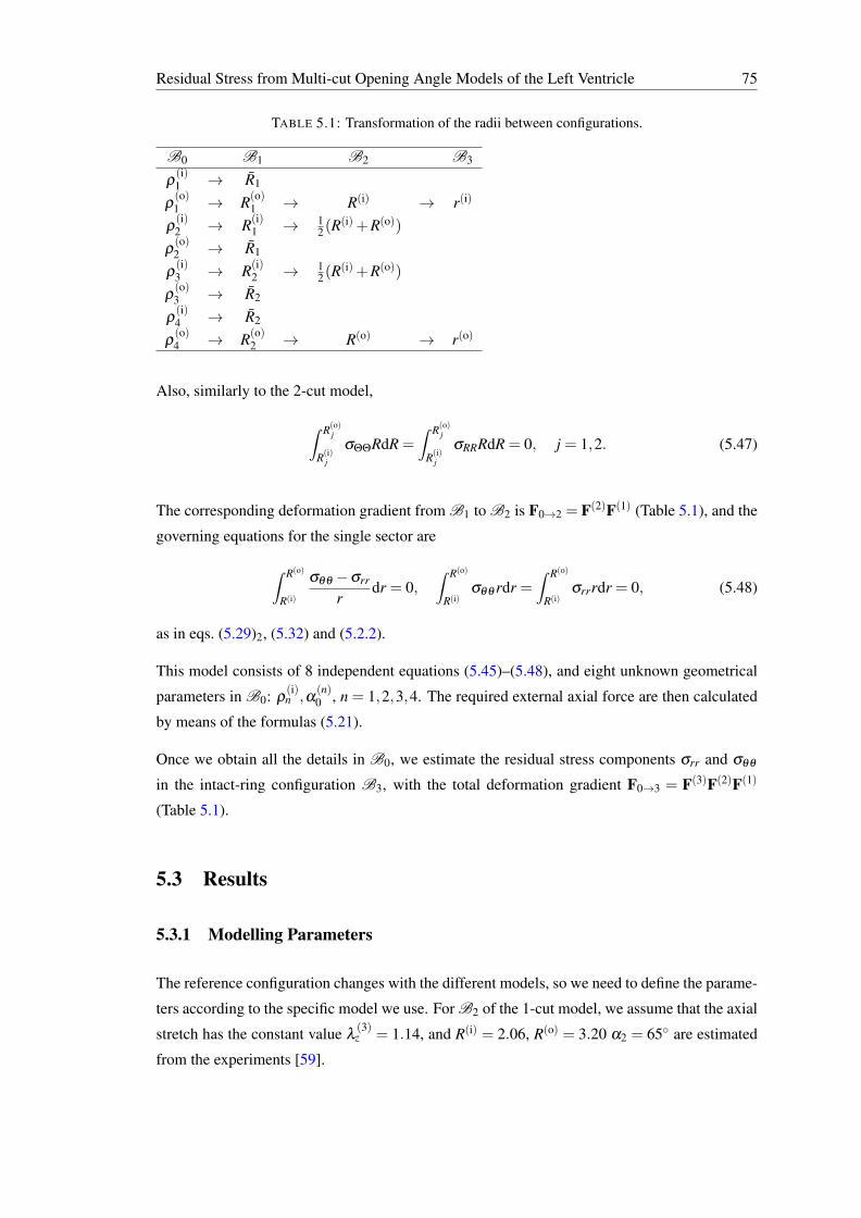
Residual Stress from Multi-cut Opening Angle Models of the Left Ventricle 75
TABLE 5.1: Transformation of the radii between configurations.
B0 B1 B2 B3
ρ(i)1 → R1
ρ(o)1 → R(o)
1 → R(i) → r(i)
ρ(i)2 → R(i)
1 → 12(R
(i)+R(o))
ρ(o)2 → R1
ρ(i)3 → R(i)
2 → 12(R
(i)+R(o))
ρ(o)3 → R2
ρ(i)4 → R2
ρ(o)4 → R(o)
2 → R(o) → r(o)
Also, similarly to the 2-cut model,
∫ R(o)j
R(i)j
σΘΘRdR =∫ R(o)
j
R(i)j
σRRRdR = 0, j = 1,2. (5.47)
The corresponding deformation gradient from B1 to B2 is F0→2 = F(2)F(1) (Table 5.1), and the
governing equations for the single sector are
∫ R(o)
R(i)
σθθ −σrr
rdr = 0,
∫ R(o)
R(i)σθθ rdr =
∫ R(o)
R(i)σrrrdr = 0, (5.48)
as in eqs. (5.29)2, (5.32) and (5.2.2).
This model consists of 8 independent equations (5.45)–(5.48), and eight unknown geometrical
parameters in B0: ρ(i)n ,α
(n)0 , n = 1,2,3,4. The required external axial force are then calculated
by means of the formulas (5.21).
Once we obtain all the details in B0, we estimate the residual stress components σrr and σθθ
in the intact-ring configuration B3, with the total deformation gradient F0→3 = F(3)F(2)F(1)
(Table 5.1).
5.3 Results
5.3.1 Modelling Parameters
The reference configuration changes with the different models, so we need to define the parame-
ters according to the specific model we use. For B2 of the 1-cut model, we assume that the axial
stretch has the constant value λ(3)z = 1.14, and R(i) = 2.06, R(o) = 3.20 α2 = 65 are estimated
from the experiments [59].
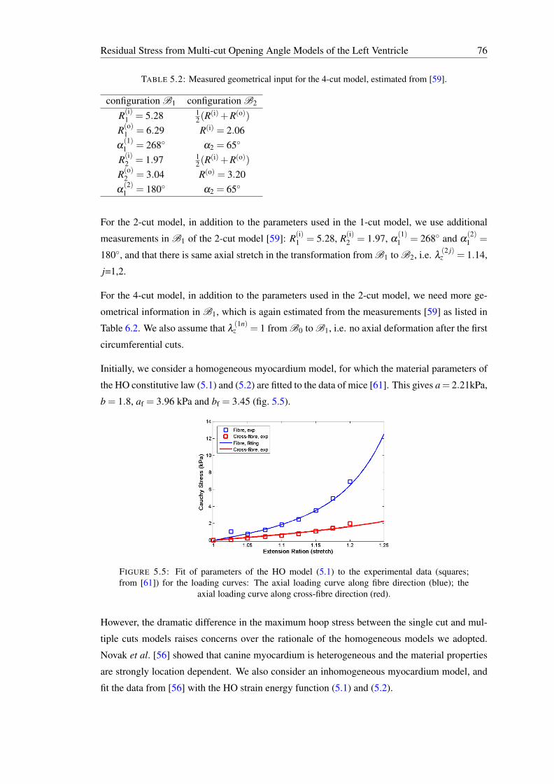
Residual Stress from Multi-cut Opening Angle Models of the Left Ventricle 76
TABLE 5.2: Measured geometrical input for the 4-cut model, estimated from [59].
configuration B1 configuration B2
R(i)1 = 5.28 1
2(R(i)+R(o))
R(o)1 = 6.29 R(i) = 2.06
α(1)1 = 268 α2 = 65
R(i)2 = 1.97 1
2(R(i)+R(o))
R(o)2 = 3.04 R(o) = 3.20
α(2)1 = 180 α2 = 65
For the 2-cut model, in addition to the parameters used in the 1-cut model, we use additional
measurements in B1 of the 2-cut model [59]: R(i)1 = 5.28, R(i)
2 = 1.97, α(1)1 = 268 and α
(2)1 =
180, and that there is same axial stretch in the transformation from B1 to B2, i.e. λ(2 j)z = 1.14,
j=1,2.
For the 4-cut model, in addition to the parameters used in the 2-cut model, we need more ge-
ometrical information in B1, which is again estimated from the measurements [59] as listed in
Table 6.2. We also assume that λ(1n)z = 1 from B0 to B1, i.e. no axial deformation after the first
circumferential cuts.
Initially, we consider a homogeneous myocardium model, for which the material parameters of
the HO constitutive law (5.1) and (5.2) are fitted to the data of mice [61]. This gives a= 2.21kPa,
b = 1.8, af = 3.96 kPa and bf = 3.45 (fig. 5.5).
FIGURE 5.5: Fit of parameters of the HO model (5.1) to the experimental data (squares;from [61]) for the loading curves: The axial loading curve along fibre direction (blue); the
axial loading curve along cross-fibre direction (red).
However, the dramatic difference in the maximum hoop stress between the single cut and mul-
tiple cuts models raises concerns over the rationale of the homogeneous models we adopted.
Novak et al. [56] showed that canine myocardium is heterogeneous and the material properties
are strongly location dependent. We also consider an inhomogeneous myocardium model, and
fit the data from [56] with the HO strain energy function (5.1) and (5.2).
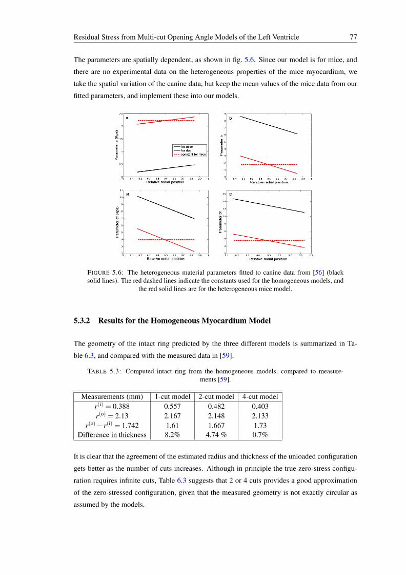
Residual Stress from Multi-cut Opening Angle Models of the Left Ventricle 77
The parameters are spatially dependent, as shown in fig. 5.6. Since our model is for mice, and
there are no experimental data on the heterogeneous properties of the mice myocardium, we
take the spatial variation of the canine data, but keep the mean values of the mice data from our
fitted parameters, and implement these into our models.
FIGURE 5.6: The heterogeneous material parameters fitted to canine data from [56] (blacksolid lines). The red dashed lines indicate the constants used for the homogeneous models, and
the red solid lines are for the heterogeneous mice model.
5.3.2 Results for the Homogeneous Myocardium Model
The geometry of the intact ring predicted by the three different models is summarized in Ta-
ble 6.3, and compared with the measured data in [59].
TABLE 5.3: Computed intact ring from the homogeneous models, compared to measure-ments [59].
Measurements (mm) 1-cut model 2-cut model 4-cut modelr(i) = 0.388 0.557 0.482 0.403r(o) = 2.13 2.167 2.148 2.133
r(o)− r(i) = 1.742 1.61 1.667 1.73Difference in thickness 8.2% 4.74 % 0.7%
It is clear that the agreement of the estimated radius and thickness of the unloaded configuration
gets better as the number of cuts increases. Although in principle the true zero-stress configu-
ration requires infinite cuts, Table 6.3 suggests that 2 or 4 cuts provides a good approximation
of the zero-stressed configuration, given that the measured geometry is not exactly circular as
assumed by the models.
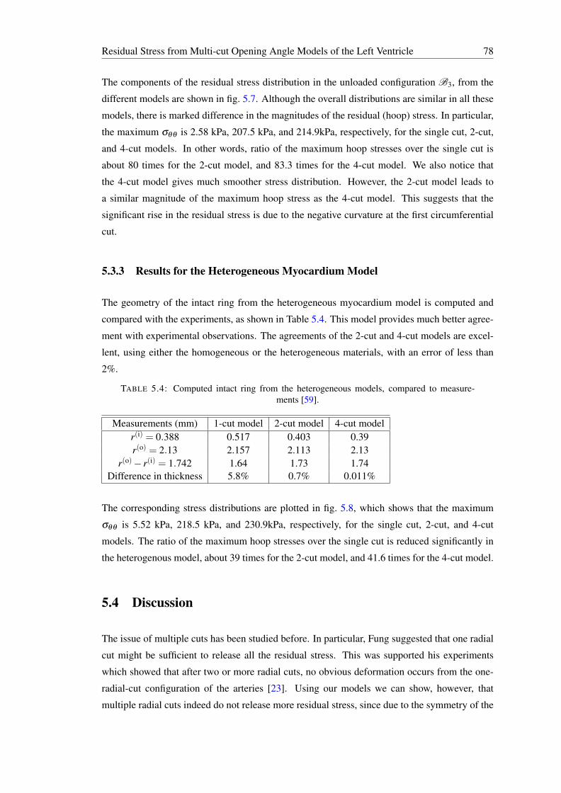
Residual Stress from Multi-cut Opening Angle Models of the Left Ventricle 78
The components of the residual stress distribution in the unloaded configuration B3, from the
different models are shown in fig. 5.7. Although the overall distributions are similar in all these
models, there is marked difference in the magnitudes of the residual (hoop) stress. In particular,
the maximum σθθ is 2.58 kPa, 207.5 kPa, and 214.9kPa, respectively, for the single cut, 2-cut,
and 4-cut models. In other words, ratio of the maximum hoop stresses over the single cut is
about 80 times for the 2-cut model, and 83.3 times for the 4-cut model. We also notice that
the 4-cut model gives much smoother stress distribution. However, the 2-cut model leads to
a similar magnitude of the maximum hoop stress as the 4-cut model. This suggests that the
significant rise in the residual stress is due to the negative curvature at the first circumferential
cut.
5.3.3 Results for the Heterogeneous Myocardium Model
The geometry of the intact ring from the heterogeneous myocardium model is computed and
compared with the experiments, as shown in Table 5.4. This model provides much better agree-
ment with experimental observations. The agreements of the 2-cut and 4-cut models are excel-
lent, using either the homogeneous or the heterogeneous materials, with an error of less than
2%.
TABLE 5.4: Computed intact ring from the heterogeneous models, compared to measure-ments [59].
Measurements (mm) 1-cut model 2-cut model 4-cut modelr(i) = 0.388 0.517 0.403 0.39r(o) = 2.13 2.157 2.113 2.13
r(o)− r(i) = 1.742 1.64 1.73 1.74Difference in thickness 5.8% 0.7% 0.011%
The corresponding stress distributions are plotted in fig. 5.8, which shows that the maximum
σθθ is 5.52 kPa, 218.5 kPa, and 230.9kPa, respectively, for the single cut, 2-cut, and 4-cut
models. The ratio of the maximum hoop stresses over the single cut is reduced significantly in
the heterogenous model, about 39 times for the 2-cut model, and 41.6 times for the 4-cut model.
5.4 Discussion
The issue of multiple cuts has been studied before. In particular, Fung suggested that one radial
cut might be sufficient to release all the residual stress. This was supported his experiments
which showed that after two or more radial cuts, no obvious deformation occurs from the one-
radial-cut configuration of the arteries [23]. Using our models we can show, however, that
multiple radial cuts indeed do not release more residual stress, since due to the symmetry of the
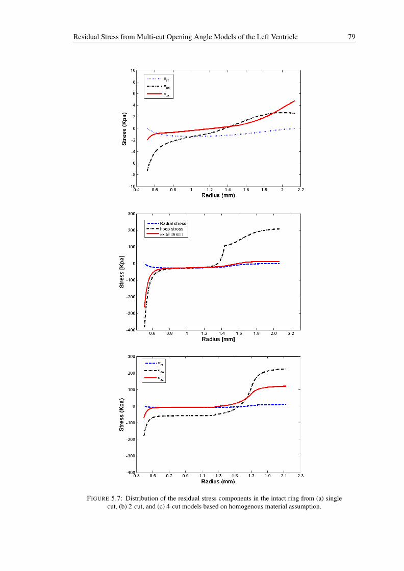
Residual Stress from Multi-cut Opening Angle Models of the Left Ventricle 79
FIGURE 5.7: Distribution of the residual stress components in the intact ring from (a) singlecut, (b) 2-cut, and (c) 4-cut models based on homogenous material assumption.
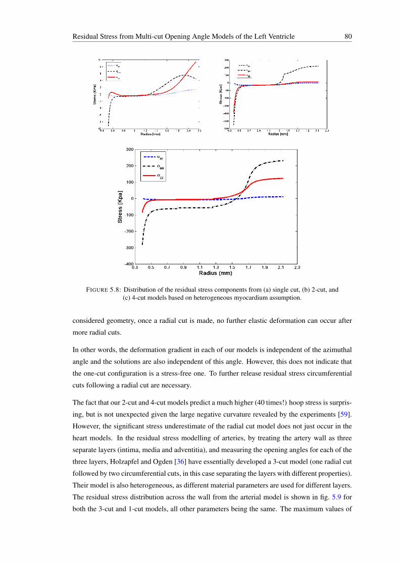
Residual Stress from Multi-cut Opening Angle Models of the Left Ventricle 80
FIGURE 5.8: Distribution of the residual stress components from (a) single cut, (b) 2-cut, and(c) 4-cut models based on heterogeneous myocardium assumption.
considered geometry, once a radial cut is made, no further elastic deformation can occur after
more radial cuts.
In other words, the deformation gradient in each of our models is independent of the azimuthal
angle and the solutions are also independent of this angle. However, this does not indicate that
the one-cut configuration is a stress-free one. To further release residual stress circumferential
cuts following a radial cut are necessary.
The fact that our 2-cut and 4-cut models predict a much higher (40 times!) hoop stress is surpris-
ing, but is not unexpected given the large negative curvature revealed by the experiments [59].
However, the significant stress underestimate of the radial cut model does not just occur in the
heart models. In the residual stress modelling of arteries, by treating the artery wall as three
separate layers (intima, media and adventitia), and measuring the opening angles for each of the
three layers, Holzapfel and Ogden [36] have essentially developed a 3-cut model (one radial cut
followed by two circumferential cuts, in this case separating the layers with different properties).
Their model is also heterogeneous, as different material parameters are used for different layers.
The residual stress distribution across the wall from the arterial model is shown in fig. 5.9 for
both the 3-cut and 1-cut models, all other parameters being the same. The maximum values of
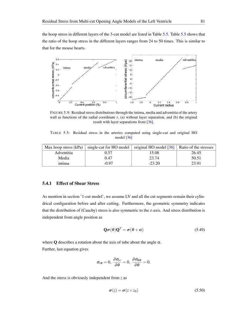
Residual Stress from Multi-cut Opening Angle Models of the Left Ventricle 81
the hoop stress in different layers of the 3-cut model are listed in Table 5.5. Table 5.5 shows that
the ratio of the hoop stress in the different layers ranges from 24 to 50 times. This is similar to
that for the mouse hearts.
FIGURE 5.9: Residual stress distributions through the intima, media and adventitia of the arterywall as functions of the radial coordinate r, (a) without layer separation, and (b) the original
result with layer separations from [36].
TABLE 5.5: Residual stress in the arteries computed using single-cut and original HOmodel [36]
Max hoop stress (kPa) single-cut for HO model original HO model [36] Ratio of the stressesAdventitia 0.57 15.08 26.45
Media 0.47 23.74 50.51intima -0.97 -23.20 23.91
5.4.1 Effect of Shear Stress
As mention in section ’1-cut model’, we assume LV and all the cut segments remain their cylin-
drical configuration before and after cutting. Furthermore, the geometric symmetry indicates
that the distribution of (Cauchy) stress is also symmetric to the z-axis. And stress distribution is
independent from angle position as
Qσ(θ)QT = σ(θ +α) (5.49)
where Q describes a rotation about the axis of tube about the angle α .
Further, last equation gives
σrθ = 0,∂σrr
∂θ= 0,
∂σθθ
∂θ= 0.
And the stress is obviously independent from z as
σ(z) = σ(z+ z0) (5.50)
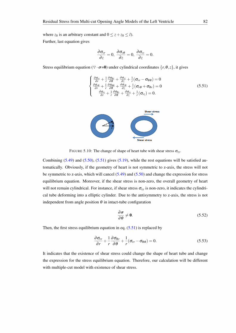
Residual Stress from Multi-cut Opening Angle Models of the Left Ventricle 82
where z0 is an arbitrary constant and 0≤ z+ z0 ≤ l).
Further, last equation gives
∂σzr
∂ z= 0,
∂σzθ
∂ z= 0,
∂σzz
∂ z= 0.
Stress equilibrium equation (O ·σ=0) under cylindrical coordinates r,θ ,z, it gives
∂σrr∂ r + 1
r∂σθr∂θ
+ ∂σzr∂ z + 1
r (σrr−σθθ ) = 0∂σrθ
∂ r + 1r
∂σθθ
∂θ+ ∂σzθ
∂ z + 1r (σrθ +σθr) = 0
∂σrz∂ r + 1
r∂σθz∂θ
+ ∂σzz∂ z + 1
r (σrz) = 0.
(5.51)
FIGURE 5.10: The change of shape of heart tube with shear stress σxy.
Combining (5.49) and (5.50), (5.51) gives (5.19), while the rest equations will be satisfied au-
tomatically. Obviously, if the geometry of heart is not symmetric to z-axis, the stress will not
be symmetric to z-axis, which will cancel (5.49) and (5.50) and change the expression for stress
equilibrium equation. Moreover, if the shear stress is non-zero, the overall geometry of heart
will not remain cylindrical. For instance, if shear stress σxy is non-zero, it indicates the cylindri-
cal tube deforming into a elliptic cylinder. Due to the antisymmetry to z-axis, the stress is not
independent from angle position θ in intact-tube configuration
∂σ
∂θ6= 0. (5.52)
Then, the first stress equilibrium equation in eq. (5.51) is replaced by
∂σrr
∂ r+
1r
∂σθr
∂θ+
1r(σrr−σθθ ) = 0. (5.53)
It indicates that the existence of shear stress could change the shape of heart tube and change
the expression for the stress equilibrium equation. Therefore, our calculation will be different
with multiple-cut model with existence of shear stress.
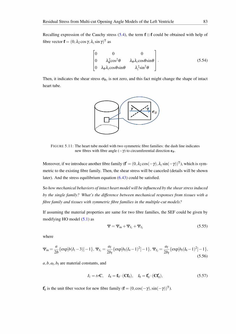
Residual Stress from Multi-cut Opening Angle Models of the Left Ventricle 83
Recalling expression of the Cauchy stress (5.4), the term f⊗ f could be obtained with help of
fibre vector f = (0,λ2 cosγ,λz sinγ)T as
0 0 0
0 λ 2θ
cos2θ λθ λzcosθsinθ
0 λθ λzcosθsinθ λ 2z sin2
θ
. (5.54)
Then, it indicates the shear stress σθz is not zero, and this fact might change the shape of intact
heart tube.
FIGURE 5.11: The heart tube model with two symmetric fibre families: the dash line indicatesnew fibres with fibre angle (−γ) to circumferential direction eθ .
Moreover, if we introduce another fibre family (f′= (0,λ2 cos(−γ),λz sin(−γ))T), which is sym-
metric to the existing fibre family. Then, the shear stress will be canceled (details will be shown
later). And the stress equilibrium equation (6.43) could be satisfied.
So how mechanical behaviors of intact heart model will be influenced by the shear stress induced
by the single family? What’s the difference between mechanical responses from tissues with a
fibre family and tissues with symmetric fibre families in the multiple-cut models?
If assuming the material properties are same for two fibre families, the SEF could be given by
modifying HO model (5.1) as
Ψ = Ψm +Ψf1 +Ψf2 (5.55)
where
Ψm =a2bexp[b(I1−3)]−1, Ψf1 =
af
2bfexp[bf(I4−1)2]−1, Ψf2 =
af
2bfexp[bf(I6−1)2]−1,
(5.56)
a,b,af,bf are material constants, and
I1 = trC, I4 = f0 · (Cf0), I6 = f′0 · (Cf′0), (5.57)
f′0 is the unit fiber vector for new fibre family (f = (0,cos(−γ),sin(−γ))T).
Residual Stress from Multi-cut Opening Angle Models of the Left Ventricle 84
The Cauchy stress tensor is then
σ =−pI+2∂Ψm
∂ I1B+2
∂Ψf1
∂ I4f⊗ f+2
∂Ψf2
∂ I4f′⊗ f′, (5.58)
Recalling (5.10), the invariants I1, I4 and I6 are given by
I1 = λ21 +λ
22 +λ
2z , I4 = λ
22 cos2
γ +λ2z sin2
γ, I6 = λ22 cos2(−γ)+λ
2z sin2(−γ), (5.59)
where the components of f and f′ are (0,λ2 cosγ,λz sinγ)T and (0,λ2 cos(−γ),λ3 sin(−γ))T,
respectively). The components of the Cauchy stress tensor in B3 are then
σrr = −p+2∂Ψm
∂ I1λ
21 , (5.60)
σθθ = −p+2∂Ψm
∂ I1λ
22 +4
∂Ψf
∂ I4λ
22 cos2
γ, (5.61)
σzz = −p+2∂Ψm
∂ I1λ
2z +4
∂Ψf
∂ I4λ
2z sin2
γ, (5.62)
σθz = 2∂Ψf
∂ I4λ2λz sinγ cosγ +2
∂Ψf
∂ I4λ2λz sin(−γ)cos(−γ) = 0. (5.63)
1-cut model with symmetric fibre families The shear stress is zero and independent from angle
position θ , it indicates the validations of (5.49) and (5.50). Therefore, with help of zero-traction
boundary condition, the stress equilibrium equation is obtained from (5.51) as
∂σrr
∂ r+
1r(σrr−σθθ ) = 0 ⇒
∫ r(o)
r(i)
σθθ −σrr
rdr = 0. (5.64)
On substitution from (5.61) and (5.62), (5.64) can be used to obtain r(i) in B3 (and r(o) from
(5.8)) when the initial radii R(i) and R(o) and k and γ are known. Hence all the Cauchy stress
components can be obtained explicitly.
1-cut model with one fibre family To test the effect of shear stress on the heart tube model, we
still assume LV and all the cut segments remain their cylindrical configurations, and then the
shear stress will be determined via stress equilibrium. This calculation will show magnitude of
shear stress and implicate the possible change of shape from a cylindrical model.
If LV and all the cut segments remain their cylindrical configurations, the components of Cauchy
stress is obtained as (5.13) to (5.16). Obviously, (5.49) and (5.49) are satisfied, which indicates
the stress equilibrium equation could be written as eq. (6.44). On substitution from ((5.13)) and
((5.14)), (5.8) can be used to obtain r(i) in B3 (and r(o) from (5.8)) when the initial radii R(i) and
R(o) and k and γ are known. Hence all the Cauchy stress components can be obtained explicitly.
2-cut model with symmetric fibre families Similarly to the 1-cut model, and with the same no-
tation for the stress components for tissues with symmetric fibre families (5.61 - 5.63), the the
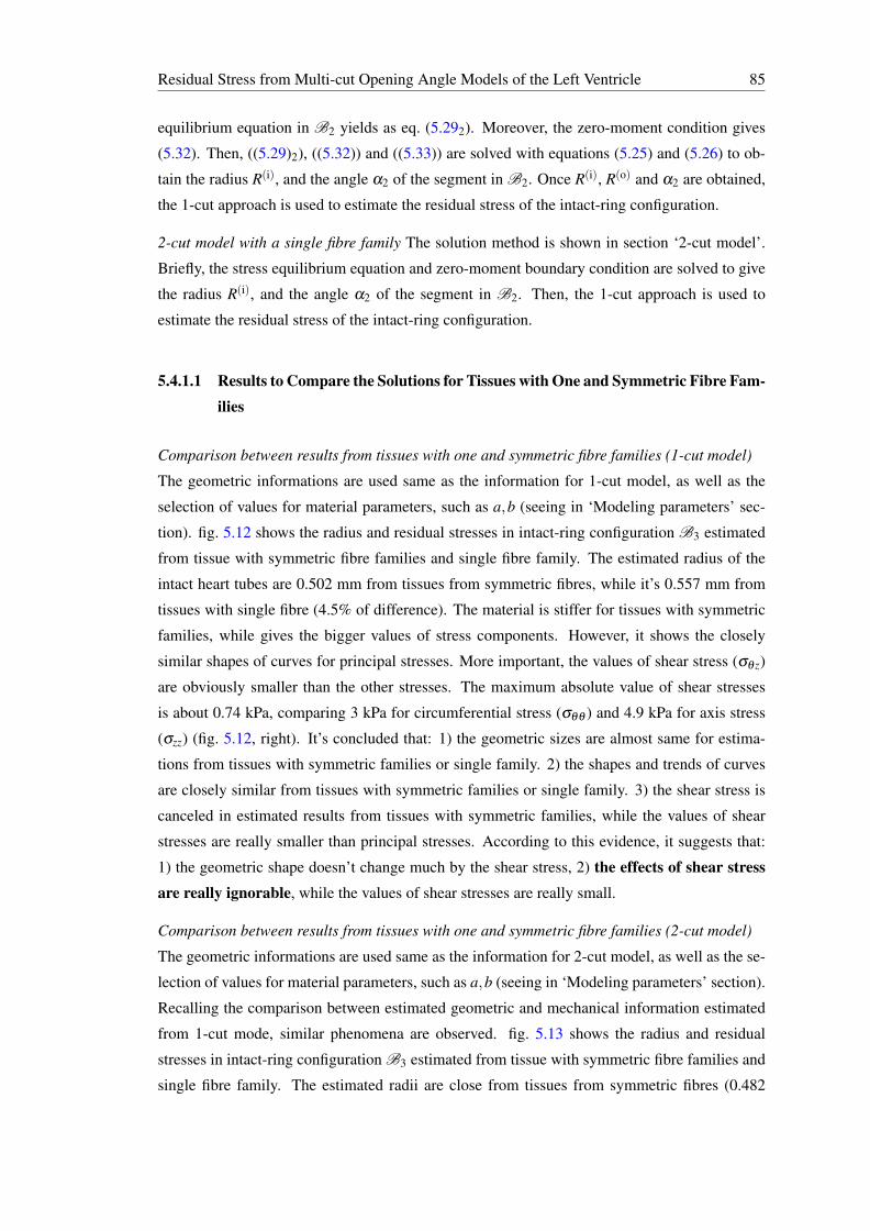
Residual Stress from Multi-cut Opening Angle Models of the Left Ventricle 85
equilibrium equation in B2 yields as eq. (5.292). Moreover, the zero-moment condition gives
(5.32). Then, ((5.29)2), ((5.32)) and ((5.33)) are solved with equations (5.25) and (5.26) to ob-
tain the radius R(i), and the angle α2 of the segment in B2. Once R(i), R(o) and α2 are obtained,
the 1-cut approach is used to estimate the residual stress of the intact-ring configuration.
2-cut model with a single fibre family The solution method is shown in section ‘2-cut model’.
Briefly, the stress equilibrium equation and zero-moment boundary condition are solved to give
the radius R(i), and the angle α2 of the segment in B2. Then, the 1-cut approach is used to
estimate the residual stress of the intact-ring configuration.
5.4.1.1 Results to Compare the Solutions for Tissues with One and Symmetric Fibre Fam-ilies
Comparison between results from tissues with one and symmetric fibre families (1-cut model)
The geometric informations are used same as the information for 1-cut model, as well as the
selection of values for material parameters, such as a,b (seeing in ‘Modeling parameters’ sec-
tion). fig. 5.12 shows the radius and residual stresses in intact-ring configuration B3 estimated
from tissue with symmetric fibre families and single fibre family. The estimated radius of the
intact heart tubes are 0.502 mm from tissues from symmetric fibres, while it’s 0.557 mm from
tissues with single fibre (4.5% of difference). The material is stiffer for tissues with symmetric
families, while gives the bigger values of stress components. However, it shows the closely
similar shapes of curves for principal stresses. More important, the values of shear stress (σθz)
are obviously smaller than the other stresses. The maximum absolute value of shear stresses
is about 0.74 kPa, comparing 3 kPa for circumferential stress (σθθ ) and 4.9 kPa for axis stress
(σzz) (fig. 5.12, right). It’s concluded that: 1) the geometric sizes are almost same for estima-
tions from tissues with symmetric families or single family. 2) the shapes and trends of curves
are closely similar from tissues with symmetric families or single family. 3) the shear stress is
canceled in estimated results from tissues with symmetric families, while the values of shear
stresses are really smaller than principal stresses. According to this evidence, it suggests that:
1) the geometric shape doesn’t change much by the shear stress, 2) the effects of shear stressare really ignorable, while the values of shear stresses are really small.
Comparison between results from tissues with one and symmetric fibre families (2-cut model)
The geometric informations are used same as the information for 2-cut model, as well as the se-
lection of values for material parameters, such as a,b (seeing in ‘Modeling parameters’ section).
Recalling the comparison between estimated geometric and mechanical information estimated
from 1-cut mode, similar phenomena are observed. fig. 5.13 shows the radius and residual
stresses in intact-ring configuration B3 estimated from tissue with symmetric fibre families and
single fibre family. The estimated radii are close from tissues from symmetric fibres (0.482
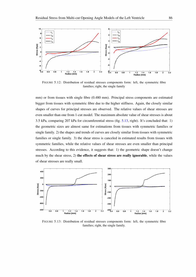
Residual Stress from Multi-cut Opening Angle Models of the Left Ventricle 86
FIGURE 5.12: Distribution of residual stresses components form: left, the symmetric fibrefamilies; right, the single family
mm) or from tissues with single fibre (0.480 mm). Principal stress components are estimated
bigger from tissues with symmetric fibre due to the higher stiffness. Again, the closely similar
shapes of curves for principal stresses are observed. The relative values of shear stresses are
even smaller than one from 1-cut model. The maximum absolute value of shear stresses is about
3.5 kPa, comparing 207 kPa for circumferential stress (fig. 5.13, right). It’s concluded that: 1)
the geometric sizes are almost same for estimations from tissues with symmetric families or
single family. 2) the shapes and trends of curves are closely similar from tissues with symmetric
families or single family. 3) the shear stress is canceled in estimated results from tissues with
symmetric families, while the relative values of shear stresses are even smaller than principal
stresses. According to this evidence, it suggests that: 1) the geometric shape doesn’t change
much by the shear stress, 2) the effects of shear stress are really ignorable, while the values
of shear stresses are really small.
FIGURE 5.13: Distribution of residual stresses components form: left, the symmetric fibrefamilies; right, the single family.
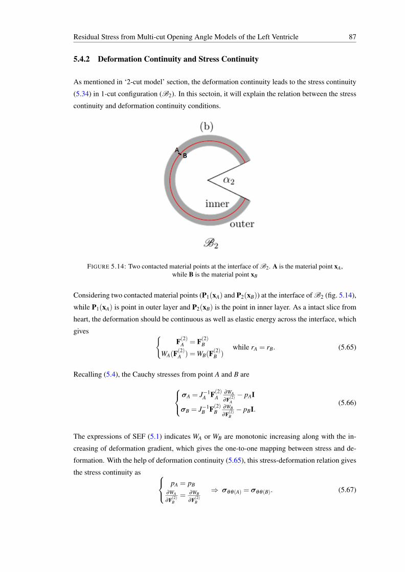
Residual Stress from Multi-cut Opening Angle Models of the Left Ventricle 87
5.4.2 Deformation Continuity and Stress Continuity
As mentioned in ‘2-cut model’ section, the deformation continuity leads to the stress continuity
(5.34) in 1-cut configuration (B2). In this sectoin, it will explain the relation between the stress
continuity and deformation continuity conditions.
FIGURE 5.14: Two contacted material points at the interface of B2. A is the material point xA,while B is the material point xB
Considering two contacted material points (P1(xA) and P2(xB)) at the interface of B2 (fig. 5.14),
while P1(xA) is point in outer layer and P2(xB) is the point in inner layer. As a intact slice from
heart, the deformation should be continuous as well as elastic energy across the interface, which
gives F(2)
A = F(2)B
WA(F(2)A ) =WB(F
(2)B )
while rA = rB. (5.65)
Recalling (5.4), the Cauchy stresses from point A and B are
σA = J−1A F(2)
A∂WA
∂F(2)A
− pAI
σB = J−1B F(2)
B∂WB
∂F(2)B
− pBI.(5.66)
The expressions of SEF (5.1) indicates WA or WB are monotonic increasing along with the in-
creasing of deformation gradient, which gives the one-to-one mapping between stress and de-
formation. With the help of deformation continuity (5.65), this stress-deformation relation gives
the stress continuity as
pA = pB∂WA
∂F(2)B
= ∂WB
∂F(2)B
⇒ σθθ(A) = σθθ(B). (5.67)
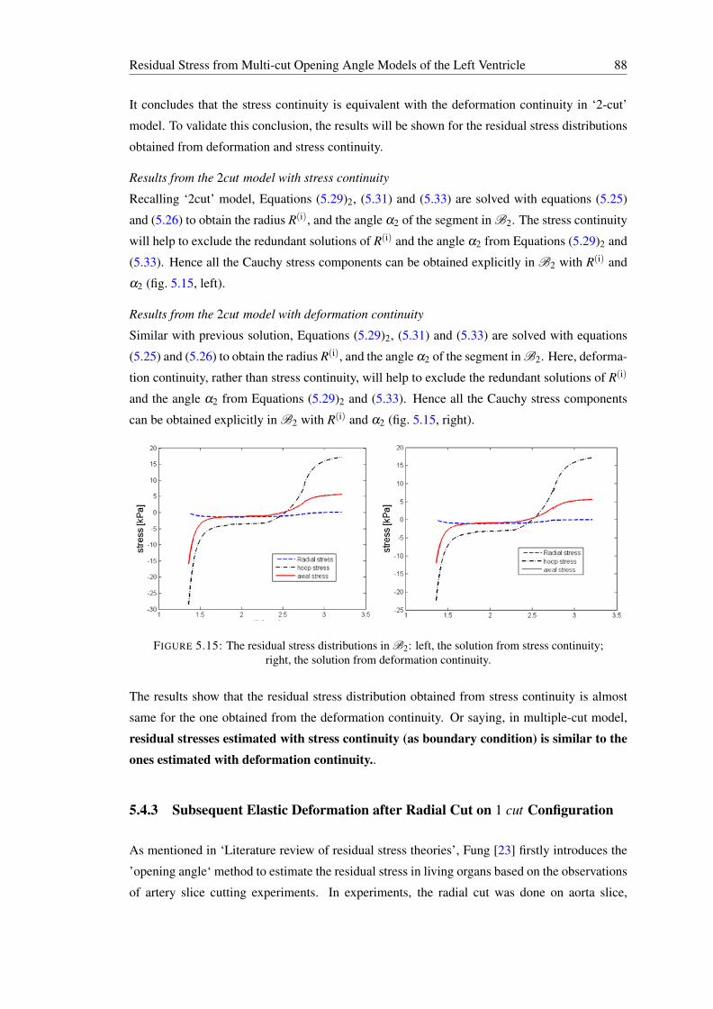
Residual Stress from Multi-cut Opening Angle Models of the Left Ventricle 88
It concludes that the stress continuity is equivalent with the deformation continuity in ‘2-cut’
model. To validate this conclusion, the results will be shown for the residual stress distributions
obtained from deformation and stress continuity.
Results from the 2cut model with stress continuity
Recalling ‘2cut’ model, Equations (5.29)2, (5.31) and (5.33) are solved with equations (5.25)
and (5.26) to obtain the radius R(i), and the angle α2 of the segment in B2. The stress continuity
will help to exclude the redundant solutions of R(i) and the angle α2 from Equations (5.29)2 and
(5.33). Hence all the Cauchy stress components can be obtained explicitly in B2 with R(i) and
α2 (fig. 5.15, left).
Results from the 2cut model with deformation continuity
Similar with previous solution, Equations (5.29)2, (5.31) and (5.33) are solved with equations
(5.25) and (5.26) to obtain the radius R(i), and the angle α2 of the segment in B2. Here, deforma-
tion continuity, rather than stress continuity, will help to exclude the redundant solutions of R(i)
and the angle α2 from Equations (5.29)2 and (5.33). Hence all the Cauchy stress components
can be obtained explicitly in B2 with R(i) and α2 (fig. 5.15, right).
FIGURE 5.15: The residual stress distributions in B2: left, the solution from stress continuity;right, the solution from deformation continuity.
The results show that the residual stress distribution obtained from stress continuity is almost
same for the one obtained from the deformation continuity. Or saying, in multiple-cut model,
residual stresses estimated with stress continuity (as boundary condition) is similar to theones estimated with deformation continuity..
5.4.3 Subsequent Elastic Deformation after Radial Cut on 1 cut Configuration
As mentioned in ‘Literature review of residual stress theories’, Fung [23] firstly introduces the
’opening angle‘ method to estimate the residual stress in living organs based on the observations
of artery slice cutting experiments. In experiments, the radial cut was done on aorta slice,
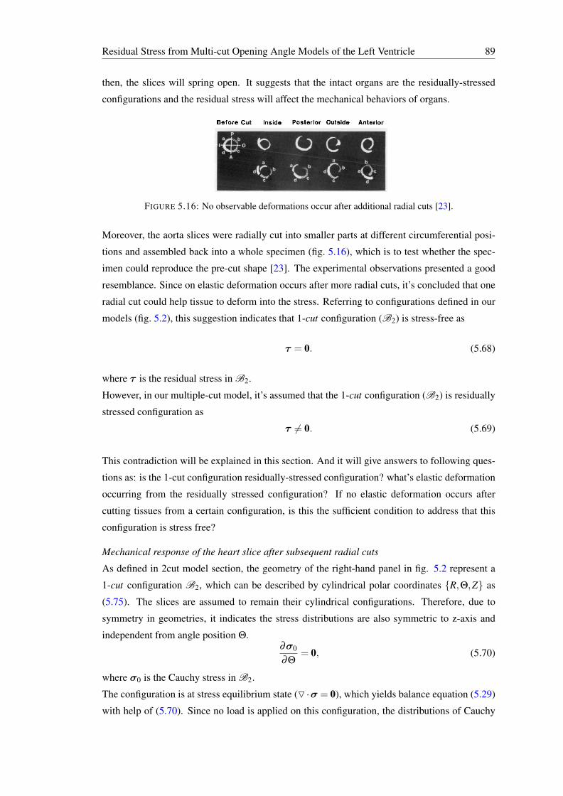
Residual Stress from Multi-cut Opening Angle Models of the Left Ventricle 89
then, the slices will spring open. It suggests that the intact organs are the residually-stressed
configurations and the residual stress will affect the mechanical behaviors of organs.
FIGURE 5.16: No observable deformations occur after additional radial cuts [23].
Moreover, the aorta slices were radially cut into smaller parts at different circumferential posi-
tions and assembled back into a whole specimen (fig. 5.16), which is to test whether the spec-
imen could reproduce the pre-cut shape [23]. The experimental observations presented a good
resemblance. Since on elastic deformation occurs after more radial cuts, it’s concluded that one
radial cut could help tissue to deform into the stress. Referring to configurations defined in our
models (fig. 5.2), this suggestion indicates that 1-cut configuration (B2) is stress-free as
τ = 0. (5.68)
where τ is the residual stress in B2.
However, in our multiple-cut model, it’s assumed that the 1-cut configuration (B2) is residually
stressed configuration as
τ 6= 0. (5.69)
This contradiction will be explained in this section. And it will give answers to following ques-
tions as: is the 1-cut configuration residually-stressed configuration? what’s elastic deformation
occurring from the residually stressed configuration? If no elastic deformation occurs after
cutting tissues from a certain configuration, is this the sufficient condition to address that this
configuration is stress free?
Mechanical response of the heart slice after subsequent radial cuts
As defined in 2cut model section, the geometry of the right-hand panel in fig. 5.2 represent a
1-cut configuration B2, which can be described by cylindrical polar coordinates R,Θ,Z as
(5.75). The slices are assumed to remain their cylindrical configurations. Therefore, due to
symmetry in geometries, it indicates the stress distributions are also symmetric to z-axis and
independent from angle position Θ.∂σ0
∂Θ= 0, (5.70)
where σ0 is the Cauchy stress in B2.
The configuration is at stress equilibrium state (O ·σ = 0), which yields balance equation (5.29)
with help of (5.70). Since no load is applied on this configuration, the distributions of Cauchy
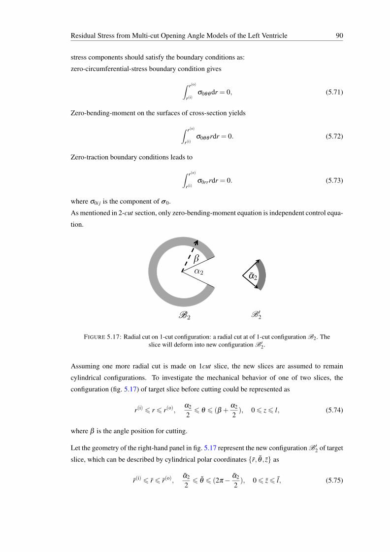
Residual Stress from Multi-cut Opening Angle Models of the Left Ventricle 90
stress components should satisfy the boundary conditions as:
zero-circumferential-stress boundary condition gives
∫ r(o)
r(i)σ0θθ dr = 0, (5.71)
Zero-bending-moment on the surfaces of cross-section yields
∫ r(o)
r(i)σ0θθ rdr = 0. (5.72)
Zero-traction boundary conditions leads to
∫ r(o)
r(i)σ0rrrdr = 0. (5.73)
where σ0i j is the component of σ0.
As mentioned in 2-cut section, only zero-bending-moment equation is independent control equa-
tion.
FIGURE 5.17: Radial cut on 1-cut configuration: a radial cut at of 1-cut configuration B2. Theslice will deform into new configuration B′2.
Assuming one more radial cut is made on 1cut slice, the new slices are assumed to remain
cylindrical configurations. To investigate the mechanical behavior of one of two slices, the
configuration (fig. 5.17) of target slice before cutting could be represented as
r(i) 6 r 6 r(o),α2
26 θ 6 (β +
α2
2), 06 z6 l, (5.74)
where β is the angle position for cutting.
Let the geometry of the right-hand panel in fig. 5.17 represent the new configuration B′2 of target
slice, which can be described by cylindrical polar coordinates r, θ , z as
r(i) 6 r 6 r(o),α2
26 θ 6 (2π− α2
2), 06 z6 l, (5.75)
Residual Stress from Multi-cut Opening Angle Models of the Left Ventricle 91
where R(i), R(o), and L denote the inner and outer radii, and the tube length, respectively, and α2
is the opening angle.
To study stress distribution in B′2, symmetry in geometry indicates the stress distributions are
also symmetric to z-axis and independent from angle position θ .
∂ σ0
∂ θ= 0 (5.76)
where σ0 is the Cauchy stress in B′2.
Stress equilibrium state (O · σ0 = 0) yields balance equation (5.29) with help of (5.76).
∫ r(o)
r(i)
σθ θ −σrr
rdr = 0, (5.77)
Similarly with previous stress state, zero load condition is applied on B′2, the distributions of
Cauchy stress components should satisfy the boundary conditions as:
zero-circumferential-stress boundary condition gives
∫ r(o)
r(i)σ0θθ dr = 0, (5.78)
Zero-bending-moment on the surfaces of cross-section yields
∫ r(o)
r(i)σ0θθ rdr = 0. (5.79)
Zero-traction boundary conditions leads to
∫ r(o)
r(i)σ0rr rdr = 0. (5.80)
where σ0i j is the component of σ0.
The stress distribution could be obtained by solving (5.79) and (equ745). The stress equilib-
rium (5.29) and boundary conditions (5.72-5.73) in B2 hold the same expressions with stress
equilibrium (5.29) and boundary conditions (5.78-5.80) in B′2. Therefore, obviously, the stress
distribution in B2 is same as one in B′2, which gives
σ0 = σ0. (5.81)
The stress energy function, respect to B2, is defined as
Ψ = Ψ(F,σ0), (5.82)
Residual Stress from Multi-cut Opening Angle Models of the Left Ventricle 92
where F is elastic deformation gradient from B2 to B′2.
Recalling (5.4), Cauchy stress in B′2 is given as
σ0 = J−1F∂ Ψ(F,σ0)
∂ F− pI. (5.83)
Since the defined SEF gives the one-to-one mapping between stress and strain, recalling (5.81),
it gives
F = I. (5.84)
Therefore, no elastic deformation occurs after more radial cuts at 1-cut configuration. More-
over, obviously, this phenomenon is independent from the cutting position. In other words, it
gives that no elastic deformation occurs after cutting at an arbitrary angle position. And this
conclusion could explain the experimental observation by Fung [23]. In the residually stressed
configuration of artery, the subsequent radial cuts don’t introduce any more elastic deformations.
Moreover, no solid evidence supports that the 1-cut configuration is the stress free configuration
for living organs. More cuts are needed to release the residual stress and address the stress-free
configuration for living organs.
If referring the non-linear elastic deformation theories to determine the stress-free configuration,
it’s safe to conclude that: if the body is at the stress-free configuration, the cuts on body will
not introduce the elastic deformation and the cut slices could perfectly reassembled back to the
previous configuration, but not vice versa; if no elastic deformation occurs after some cuts on
the body, the initial configuration is not necessary to be the stress-free one.
5.5 Conclusion
Based on experimental observations, it shows that a single radial cut does not release all residual
stress. We have developed multiple cuts models to estimate the residual stress distributions in a
mouse LV model. Our results show that both radial cuts and circumferential cuts are required
to release the residual stresses in the left ventricle. Remarkably, using radial cuts alone leads to
significantly underestimated residual stress, which will be around 40 times greater if estimated
properly. We show that similar findings apply to arteries [36].
Comparing the stress distritubtions in intact rings, it shows stresses estimated by 4-cut model are
smoother than by 2-cut model. In real heart, the stresses should smoothly distribute for intact
heart, which indicates 4-cut model is more reasonable. Moreover, as mentioned in previous
researches, it suggests ‘infinite cuts’ are efficient to release all residual stress in living organs,
since residual stress is induced by the complex (inhomogeneous) growth. Therefore, 4-cut model
may give better estimations for residual stress.
Residual Stress from Multi-cut Opening Angle Models of the Left Ventricle 93
The mechanical behaviors of LV are calculated with the single fibre family. According to the
discussion about effect of shear stress on the mechanical response of LV tube, it shows that the
geometric shape doesn’t change much by the shear stress. Therefore, the effects of shear stress
are really ignorable, while the values of shear stresses are really small.
The stress distributions in 1cut configuration are obtained from both stress and deformation
continuity conditions. And it shows that stress continuity is almost equivalent with deformation
continuity in multiple-cut model.
The computation results explain experimental observation by Fung [23]. In the residually
stressed configuration of artery, the subsequent radial cuts don’t introduce any more elastic de-
formations. Moreover, no solid evidence supports that the 1-cut configuration is the stress free
configuration for living organs. More cuts are needed to release the residual stress and address
the stress-free configuration for living organs.
Moreover, magnitude of hoop stress is estimated to be larger than the order of active tension
(200 kPa from this work V S 100 kPa for normal active tension for human heart). It might
be explained by: 1) the selection of the material properties. The constitutive parameters are
fitted from the experiments on rice [61], while the opening angles are obtained from the exper-
iments [59]. Considering the diversity of mechanical behaviors of soft tissues, the constitutive
parameters might be different between two mentioned works, even though these are the closest
data according to author’s best knowledge. With lower values for constitutive parameters, the
magnitudes of hoop stress will be significantly lower. For instance, if af is used as value of
2.00kPa in equation (5.2) (rather than 3.96kPa from parameter fitting), the max hoop stress is
reduced to 114 kPa (53% lower than estimation from previous results). 2) the time effects on the
opening angle; as mentioned in [30], the opening angle will be enlarged under the viscoelasticity
effects of (in vitro) artery tissues after the arterial samples are separated from the living organs.
In experiments [59], the opening angles after circumferential cuts are not immediately measured
after heart harvesting, which might introduce the enlarged opening angle. This fact (enlarged
opening angle) leads to the overestimated residual stresses.
This work gives a new direction to estimate the residual stress in LV by using the multiple cut
model. As shown in previous experiments (like [59]), single cut can release all the residual
stress in LV, since further deformations are observed after more cuts. By simply estimating
the residual with one-cut model, the residual stress will be significantly underestimated. To
increase the accuracy of the residual stress estimations. More experimental data are needed to
describe the material properties of in vitro tissues. Besides, the constitutive law, involving the
viscoelasticity in soft tissues, could be employed to estimate the residual stress in living organs.
Chapter 6
A Coupled Agent-based andHyperelastic Modelling of the LeftVentricle Post Myocardial Infarction
6.1 Introduction
Myocardial infarction (MI), commonly known as a heart attack, occurs when blood flow de-
creases or stops to a part of the heart, causing damage to the heart muscle. The healing process
in the heart poses a complex multiscale soft tissue problem, invovling cardiac growth and remod-
elling (G&R). Cellular growth is often considered to be the cause for residual stress [72]. The
myocardial stress and constitutive properties are the two key factors in myocardial G&R [91].
There are typically two types of G&R modelling approaches at the continuum level. One is
the volumetric growth (the density remains unchanged) following the G&R, and the other is the
density growth (volume remains unchanged). In the volumetric approach, G&R can be modelled
using the growth tensor first introduced by Rodriguez et al. [65]. For example, Goketepe et al.
[25] developed a multi-scale framework to study myocardial growth via alignment of myocytes
and parallel additional of sarcomere units. Their model was extended to study the mechanical ef-
fects on remodelling patterns of left ventricle (LV) after certain surgical procedures. Kerckhoffs
et al. [47] developed a strain-driven growth laws to explain how the grown cardiac myocytes
increased the fibre and cross-fibre strains . Density growth, on the other hand, focuses on chang-
ing the constitutive properties of myocaridum in healthy remote and infarcted cardiac tissues,
the latter being characterised with stiffer constitutive properties, simulating the replacement of
fibrosis by collagen fibres. For example, in a study, the stiffness in the infarct zone is increased
significantly compared to functional myocardium in a patient-specific infarcted LV model.
94
A coupled agent-based and hyperelastic modelling of the left ventricle post myocardialinfarction 95
There are very few combined volumetric and density growth models for G&R, particularly for
the heart. Eriksson et al. [16] developed a framework to study the G&R process of fibre-
reinforced arteries, while the evolution of constitutive properties was simulated via a density-
and-volumetric growth approach for a mixture of constituents. However, the remodelling of
the fibre structure was not included. Indeed, it is not clear how the collagen fibre structure is
modified during the post-MI healing process, and how the macro-mechanical response of the
infarcted LV changes post-MI.
Recent developments in soft tissue modelling in parallel with advances in experimental tech-
niques have enabled us to predict mechanical states at, and obtain images of, the small scales
relevant to biology. For example, the structure-based fibre-reinforced Holzapfel–Ogden model
(HO) [35] for myocardium was developed based on simple shear experiments, and has catalysed
much of the recent activities in soft tissue modelling.
At the cellular level, collagen deposition and remodelling are regulated by fibroblast cell align-
ment. Environmental cues, such as mechanical and chemical cues, have been shown to influence
cell migration and regulate the micro-fibre structures [12]. Recently, agent-based models that
account for these effects have been developed and used to study a two-dimensional slab model
of the myocardium infarction [18, 66]. However, the extension of this approach to a three-
dimensional LV model has not been reported.
In this paper, we combine the agent-based approach by [18, 66] with a structure-based fibre-
reinforced constitutive law to study MI healing in a three-dimensional left ventricular model
for the first time. To account for the necessarily dispersed fibre structure post-MI, we mod-
ify the original Holzapfel–Ogden (HO) constitutive law [35] by employing a distributed fibre
model [37]. The specific fibre distribution is determined using an agent-based model similar
to that of [18]. We then incorporate the agent-based model within a finite element (FE) LV
model. This new multiscale model is used to simulate the myocardium remodelling in terms of
the collagen fibre structure and density. To account for the micro-fibre structure in the tissue
constitutive laws, a commonly used up-scaling method is based on volumetric averaging [83].
However, since these micro-fibres in the soft tissue do not support compression, a switch is re-
quired to exclude the compressed fibres. For dispersed fibre structure, however, such a ‘switch’
is often applied inappropriately due to the volumetric averaging [37]. In our model, we describe
the fibre structure using angular integration over a local coordinate system, which allows an
analytical expression of the fibre on-off switch to be implemented in the constitutive model.
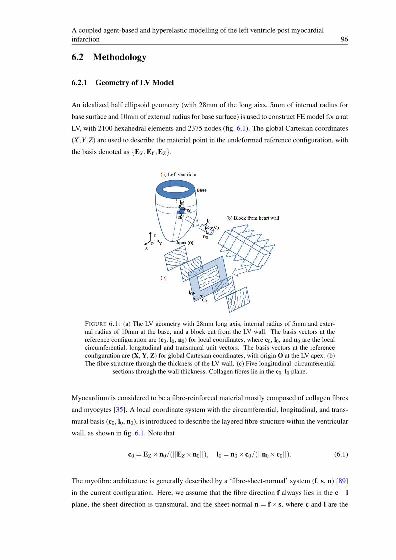
A coupled agent-based and hyperelastic modelling of the left ventricle post myocardialinfarction 96
6.2 Methodology
6.2.1 Geometry of LV Model
An idealized half ellipsoid geometry (with 28mm of the long aixs, 5mm of internal radius for
base surface and 10mm of external radius for base surface) is used to construct FE model for a rat
LV, with 2100 hexahedral elements and 2375 nodes (fig. 6.1). The global Cartesian coordinates
(X ,Y,Z) are used to describe the material point in the undeformed reference configuration, with
the basis denoted as EX ,EY ,EZ.
FIGURE 6.1: (a) The LV geometry with 28mm long axis, internal radius of 5mm and exter-nal radius of 10mm at the base, and a block cut from the LV wall. The basis vectors at thereference configuration are (c0, l0, n0) for local coordinates, where c0, l0, and n0 are the localcircumferential, longitudinal and transmural unit vectors. The basis vectors at the referenceconfiguration are (X, Y, Z) for global Cartesian coordinates, with origin O at the LV apex. (b)The fibre structure through the thickness of the LV wall. (c) Five longitudinal–circumferential
sections through the wall thickness. Collagen fibres lie in the c0–l0 plane.
Myocardium is considered to be a fibre-reinforced material mostly composed of collagen fibres
and myocytes [35]. A local coordinate system with the circumferential, longitudinal, and trans-
mural basis (c0, l0, n0), is introduced to describe the layered fibre structure within the ventricular
wall, as shown in fig. 6.1. Note that
c0 = EZ×n0/(||EZ×n0||), l0 = n0× c0/(||n0× c0||). (6.1)
The myofibre architecture is generally described by a ‘fibre-sheet-normal’ system (f, s, n) [89]
in the current configuration. Here, we assume that the fibre direction f always lies in the c− lplane, the sheet direction is transmural, and the sheet-normal n = f× s, where c and l are the
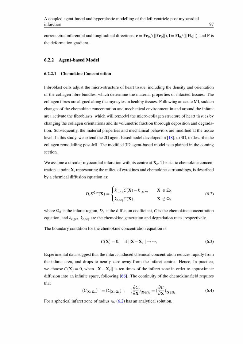
A coupled agent-based and hyperelastic modelling of the left ventricle post myocardialinfarction 97
current circumferential and longitudinal directions: c = Fc0/(||Fc0||), l = Fl0/(||Fl0||), and F is
the deformation gradient.
6.2.2 Agent-based Model
6.2.2.1 Chemokine Concentration
Fibroblast cells adjust the micro-structure of heart tissue, including the density and orientation
of the collagen fibre bundles, which determine the material properties of infacted tissues. The
collagen fibres are aligned along the myocytes in healthy tissues. Following an acute MI, sudden
changes of the chemokine concentration and mechanical environment in and around the infarct
area activate the fibroblasts, which will remodel the micro-collagen structure of heart tissues by
changing the collagen orientations and its volumetric fraction thorough deposition and degrada-
tion. Subsequently, the material properties and mechanical behaviors are modified at the tissue
level. In this study, we extend the 2D agent-basedmodel developed in [18], to 3D, to describe the
collagen remodelling post-MI. The modified 3D agent-based model is explained in the coming
section.
We assume a circular myocardial infarction with its centre at Xc. The static chemokine concen-
tration at point X, representing the milieu of cytokines and chemokine surroundings, is described
by a chemical diffusion equation as:
Dc∇2C(X) =
kc,degC(X)− kc,gen, X ∈Ωb
kc,degC(X), X /∈Ωb
(6.2)
where Ωb is the infarct region, Dc is the diffusion coefficient, C is the chemokine concentration
equation, and kc,gen, kc,deg are the chemokine generation and degradation rates, respectively.
The boundary condition for the chemokine concentration equation is
C(X) = 0, if ||X−Xc|| → ∞, (6.3)
Experimental data suggest that the infarct-induced chemical concentration reduces rapidly from
the infarct area, and drops to nearly zero away from the infarct centre. Hence, In practice,
we choose C(X) = 0, when ||X−Xc|| is ten times of the infarct zone in order to approximate
diffusion into an infinite space, following [66]. The continuity of the chemokine field requires
that
(C|X∈Ωb)+ = (C|X∈Ωb)
−, (∂C∂X
)+|X∈Ωb= (
∂C∂X
)−|X∈Ωb(6.4)
For a spherical infarct zone of radius r0, (6.2) has an analytical solution,
C(r) =
a1exp(a2r)−a1exp(−a2r)r +a0, r ≤ r0
a3exp(−a2r)r , r > r0
(6.5)
where a0 = kc,gen/kc,deg, a1 =−a0(r0+1/a2)2exp(a2r0)
, a2 =√
kc,deg/Dc and a3 =12(r0−1/a2)exp(a2r0)−
a1.
The fibroblast activation parameters, including cell migration speed, collagen degradation rate,
collagen deposition rate and collagen reorientation rate, all are modulated by the local chemokine
concentration C(r). To compute the activation parameters in the agent based model, the local
fibroblast activation parameters are assumed to vary linearly with C as
Pi(X) = (Pi,max−Pi,min
Cmax−Cmin) [C(X)−Cmin]+Pi,min (6.6)
where Pi is the ith rate parameter, Pi,max and Pi,min are the maximum and minimum rates, and
Cmax, Cmin are the maximum and minimum chemokine concentrations.
6.2.2.2 Fibroblast Migrations Regulated by Environmental Cues
According to the experimental observations in [18], the infarct area is stretched only into lon-
gitudinal and circumferential directions and developed the scar tissues with collagen fibres. In
this thesis, it’s assumed that the new collagen fibres are disposed in the c-l plane, along with
the fibroblast migrations regulated by local environmental cues. These include the chemical,
mechanical, persistent and structural cues ([12], [18], [66]. We further assume the fibroblasts
are rigid discs with radius Rcell , and there is no interaction between fibroblasts [66].
Chemical Cues
We define chemokine vector as the production of chemokine concentration and the outward
normal vector at the fibroblast boundary. The chemical cue vcis obtained from
vc =1
2π
∫π
−π
C(r)n(θ)dθ , (6.7)
where n(θ) is the unit outward normal vector of the cell boundary in the current configuration,
r is the distance at the boundary of a fibroblast cell to the infarction centre Xc.
Mechanical Cues
The mechanical cue vm is defined as
vm =1
2π
∫π
−π
εn(ξ )n(θ) dθ (6.8)
where εn = n ·Dn is the normal strain, and
D =12(I−F−T F−1),
is the Eulerian strain tensor, F is the deformation gradient, ξ is the material point at the cell
boundary, and I is the identify matrix.
Structural Cues
The structural cue vs is defined as
vs =
∫N(θ)f(θ) dθ∫
N(θ)dθ, (6.9)
where N(θ) is the number of collagen fibres along angle θ , f(θ) is the unit vector along θ in the
current configuration, f = Ff0/||Ff0|| and f0 = cos(θ)c0 + sin(θ)l0.
Persistence Cue
The persistent cue vp, is defined as the fibroblast cell migration velocity
vp = Scell(X)u(Θ), (6.10)
where Θ is the angle of fibroblast migration at time t, Scell is the value of the fibroblast migration
speed, and u(Θ) is the unit vector along Θ in the current configuration, u = Fu0/||Fu0|| and
u0 = cosΘ c0 + sinΘ l0.
The fibroblast position at time t is tracked from
x(t) =∫ t
t0vpdt. (6.11)
Resultant Cue
The fibroblast resultant cue ρ is a weighted and normalised sum of all the cues (6.7 – 6.10),
ρ=∑ci
η +∑ ||ci||, ci =
Wi
Mivi, (6.12)
where vi is the ith cue vector, ci is the ith normalized and weighted cue vector, Mi and Wi are
ith scaling and weighting factors, and η is the persistent tuning factor, which is constant fitted
from experimental observations [66]. The orientation of ρ provides the mean fibre angle Θ. We
assume that the fibroblasts obey a Von mises distribution,
ϕVM(Θ|Θ,σ) =eσcos(Θ−Θ)
I0(σ), σ
2 =−2ln||ρ||,σ2 =−2ln||ρ||, (6.13)
where I0 is the Bessel function of the first kind of order zero.
FIGURE 6.2: A) The resultant cue that represents the mean fibroblast direction is computedfrom a weighted combination of all cues; B) the von Mises distribution of the fibroblast orien-
tation.
6.2.2.3 Remodeling of the Collagen Fibre Structure
The collagen structure of healthy tissue is described by the quantity of collagen fibres (N0tot) and
the fibre angles. And the statistical feature of fibre angles can be described by a fibre orientation
density function (ϕ0). Then, during the healing process of infarction, more collagen fibres will
be deposed by fibroblast cells, while the fibre angles are also updated. The numerical strategy is
explained in this section how to mathematically describe the evolution the statistical features of
fibre family at the arbitrary material point in infarction region.
The local collagen fibre distribution in the current configuration are remodelled by fibroblasts in
the following way.
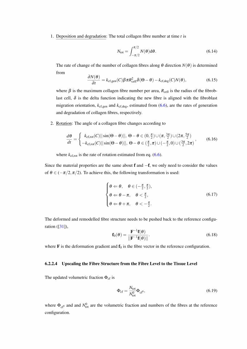
1. Deposition and degradation: The total collagen fibre number at time t is
Ntot =∫
π/2
−π/2N(θ)dθ . (6.14)
The rate of change of the number of collagen fibres along θ direction N(θ) is determined
from∂N(θ)
∂ t= kcf,gen(C)βπR2
cellδ (Θ−θ)− kcf,deg(C)N(θ), (6.15)
where β is the maximum collagen fibre number per area, Rcell is the radius of the fibrob-
last cell, δ is the delta function indicating the new fibre is aligned with the fibroblast
migration orientation, kcf,gen and kcf,deg, estimated from (6.6), are the rates of generation
and degradation of collagen fibres, respectively.
2. Rotation: The angle of a collagen fibre changes according to
dθ
dt=
kcf,rot(C)||sin(Θ−θ)||, Θ−θ ∈ (0, π
2 )∪ (π, 3π
2 )∪ (2π, 5π
2 )
−kcf,rot(C)||sin(Θ−θ)||, Θ−θ ∈ (π
2 ,π)∪ (−π
2 ,0)∪ (3π
2 ,2π), (6.16)
where kcf,rot is the rate of rotation estimated from eq. (6.6).
Since the material properties are the same about f and −f, we only need to consider the values
of θ ∈ (−π/2,π/2). To achieve this, the following transformation is used:
θ ⇐ θ , θ ∈ (−π
2 ,π
2 ),
θ ⇐ θ −π, θ < π
2 ,
θ ⇐ θ +π, θ <−π
2 .
(6.17)
The deformed and remodelled fibre structure needs to be pushed back to the reference configu-
ration ([31]),
f0(θ) =F−1f(θ)||F−1f(θ)|| . (6.18)
where F is the deformation gradient and f0 is the fibre vector in the reference configuration.
6.2.2.4 Upscaling the Fibre Structure from the Fibre Level to the Tissue Level
The updated volumetric fraction Φcf is
Φcf =Ntot
N0tot
Φcf0 , (6.19)
where Φcf0 and and N0tot are the volumetric fraction and numbers of the fibres at the reference
configuration.
The fibre orientation density function, when pushed back to the reference configuration, is esti-
mated from
ϕ(θ) = πN(θ)
Ntot. (6.20)
6.2.3 Constitutive Laws for Myocardium
6.2.3.1 Modified HO Model with Fibre Orientation Density Function
For the remote healthy myocardium (r(X)> r0), we use the standard HO model [35], i.e.
Ψ = Ψm +Ψcf, (6.21)
where
Ψm =a2bexp [b(I1−3]−1 , Ψcf =
acf
2bcf
exp[bcf(I4(θ)−1)2]−1
, (6.22)
in which a,b acf, bcf are material parameters, and I1, I4 are the invariants of the right Cauchy–
Green tensor ~C = ~FT~F ,
I1 = ~C : I, I4 = u0(θ) ·Cu0(θ), (6.23)
Here ‘:’ denotes a double contraction, and u0(θ) = cosθ c0 + sinθ l0.
To describe the mechanical behavior of the infarcted tissue (r(X) ≤ r0), we modify the HO
model as
Ψ = Φm,tΨm +Φcf,tΨcf, (6.24)
where Φm,t(= 1−Φcf,y) is the volume fraction of the ground matrix, Ψm is the same as in (6.22)
but Ψcf is changed to
Ψcf =1π
acf
2bcf
∫
Σ
exp[bcf(I4(θ)−1)2]−1
ϕt(θ) dθ . (6.25)
Notice that the integration in (6.25) is over a domain Σ in which the fibres are in tension, not
(−π/2,π/2). This is because collagen fibres bear load only when they are stretched. We will
address this point in Section 2.3.2.
A rule-based myocardium fibre generation algorithm is adopted to describe the local mean fibre
angle. We first calculate the normalized distance parameter d for an arbitrary material point Xas
d =dendo
dendo +depi, (6.26)
FIGURE 6.3: The shadowed areas show the range of Σ of stretched collagen fibres within−π
2 < θ < π
2 for selected scenarios (dash line denotes I4 = 1): (a) case 1, C23 > 0; (b) case 2,C33−1 > 0,∆≤ 0; (c) case 2, C33−1 > 0,∆ > 0; (d) case 2, C33−1 < 0,∆ > 0.
where dendo, depi are the distances from X to the endocardial and epicardial surfaces. Then, the
local mean fibre angle θ0 at X is defined as
θ0 = θmax(1−2d),
where θmax = π/3, since it has been observed that the mean angle of fibres in a healthy left
ventricle rotates transmurally across the heart wall from π/3 at the endocardial surface to −π/3
at the epicardial surface [51].
6.2.3.2 Exclusion of the Compressed Fibres
To exclude the compressed fibres, we choose Σ in eq. (6.25) so that
I4 > 1, or (C22−1)cos2θ +2C23 sinθ cosθ +(C33−1)sin2
θ > 0, (6.27)
where Ci j are the Cartesian components of C. Eq. (6.27) gives the range of Σ for the stretched
collagen fibres in the following two cases.
• Case 1: C33 = 1,
Σ =
(θ1,π
2 ), C23 > 0
(−π
2 ,θ1), C23 < 0
(−π
2 ,π
2 ), C23 = 0, C22 > 1
∅, C23 = 0, C22 < 1
(6.28)
where θ1 = arctan 1−C222C23
.
• Case 2:
Σ =
(−π
2 ,π
2 ), C33−1 > 0, ∆≤ 0,
(−π
2 ,θ2) ∪ (θ3,π
2 ), C33−1 > 0, ∆ > 0
(θ2,θ3), C33−1 < 0, ∆ > 0
∅, C33−1 < 0, ∆ < 0
(6.29)
where ∆ = (2C23)2−4(C33−1)(C22−1), and θ2 and θ3 are the roots of (6.27).
The Cauchy stress is then
σ =−pI+F∂Ψ
∂ I1
∂ I1
∂F+F
∂Ψ
∂ I4
∂ I4
∂F
=−pI+Φm,t a exp[b(I1−3)]B
+1π
Φcf
∫
Σ
2acf(I4−1)exp[bcf(I4−1)2]ϕ(θ)u(θ)⊗u(θ)dθ ,
(6.30)
where B = FFT is the left Cauchy-Green deformation tensor.
6.2.3.3 Change of Basis from Cartesian to Local Coordinates
In numerical simulation, the Cartesian coordinates are usually employed to describe the de-
formation of material point X, which indicates that the deformation tensor F is defined with
Cartesian base ei. However, the fibre family is described by a local coordinate system (c0, l0.
In order to exclude the compressed fibres, it is convenient to transform the description of fibre
orientation between the global Cartesian coordinates and the local polar coordinates, namely,
x∗ = Qx, (6.31)
where * indicates the corresponding variable in the local coordinate, and Q is the rotation tensor
(Q = f⊗ e1 + c⊗ e2 + l⊗ e3).
Then the local deformation gradient and right Cauchy–Green tensor are given as
F∗ = QF, C∗ = Q · (FT F)QT . (6.32)
TABLE 6.1: fitted material parameters for myocardium from [61, 66].
Initial volumetric fractions Φm,t0 = 0.97 Φcf,t0 = 0.03Initial concentration parameter σ0 = 9.10
matrix parameters a = 2.28 kPa b = 1.8Collagen parameters acf = 132.0 kPa bcf = 3.45
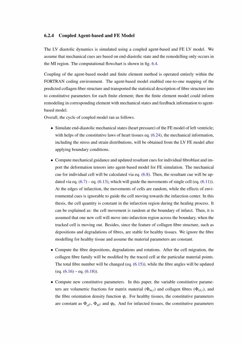
6.2.4 Coupled Agent-based and FE Model
The LV diastolic dynamics is simulated using a coupled agent-based and FE LV model. We
assume that mechanical cues are based on end-diastolic state and the remodelling only occurs in
the MI region. The computational flowchart is shown in fig. 6.4.
Coupling of the agent-based model and finite element method is operated entirely within the
FORTRAN coding environment. The agent-based model enabled one-to-one mapping of the
predicted collagen fiber structure and transported the statistical description of fibre structure into
to constitutive parameters for each finite element; then the finite element model could inform
remodeling in corresponding element with mechanical states and feedback information to agent-
based model.
Overall, the cycle of coupled model ran as follows.
• Simulate end-diastolic mechanical states (heart pressure) of the FE model of left ventricle;
with helps of the constitutive laws of heart tissues eq. (6.24), the mechanical information,
including the stress and strain distributions, will be obtained from the LV FE model after
applying boundary conditions.
• Compute mechanical guidance and updated resultant cues for individual fibroblast and im-
port the deformation tensors into agent-based model for FE simulation. The mechanical
cue for individual cell will be calculated via eq. (6.8). Then, the resultant cue will be up-
dated via eq. (6.7) – eq. (6.13), which will guide the movements of single cell (eq. (6.11)).
At the edges of infarction, the movements of cells are random, while the effects of envi-
ronmental cues is ignorable to guide the cell moving towards the infarction center. In this
thesis, the cell quantity is constant in the infarction region during the healing process. It
can be explained as: the cell movement is random at the boundary of infarct. Then, it is
assumed that one new cell will move into infarction region across the boundary, when the
tracked cell is moving out. Besides, since the feature of collagen fibre structure, such as
depositions and degradations of fibres, are stable for healthy tissues. We ignore the fibre
modelling for healthy tissue and assume the material parameters are constant.
• Compute the fibre depositions, degradations and rotations. After the cell migration, the
collagen fibre family will be modified by the traced cell at the particular material points.
The total fibre number will be changed (eq. (6.15)), while the fibre angles will be updated
(eq. (6.16) – eq. (6.18)).
• Compute new constitutive parameters. In this paper, the variable constitutive parame-
ters are volumetric fractions for matrix material (Φm,t) and collagen fibres (Φcf,t), and
the fibre orientation density function ϕt . For healthy tissues, the constitutive parameters
are constant as Φcf0 , Φm0 and ϕ0. And for infarcted tissues, the constitutive parameters
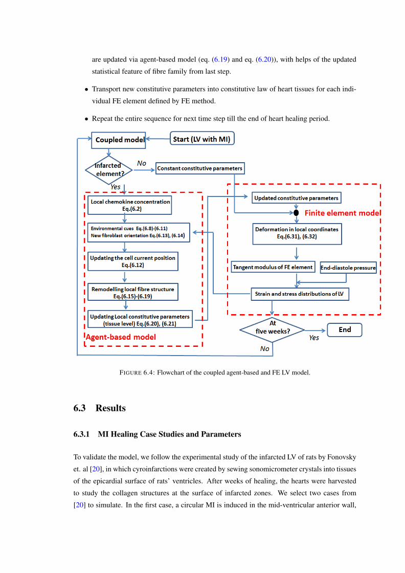
are updated via agent-based model (eq. (6.19) and eq. (6.20)), with helps of the updated
statistical feature of fibre family from last step.
• Transport new constitutive parameters into constitutive law of heart tissues for each indi-
vidual FE element defined by FE method.
• Repeat the entire sequence for next time step till the end of heart healing period.
FIGURE 6.4: Flowchart of the coupled agent-based and FE LV model.
6.3 Results
6.3.1 MI Healing Case Studies and Parameters
To validate the model, we follow the experimental study of the infarcted LV of rats by Fonovsky
et. al [20], in which cyroinfarctions were created by sewing sonomicrometer crystals into tissues
of the epicardial surface of rats’ ventricles. After weeks of healing, the hearts were harvested
to study the collagen structures at the surface of infarcted zones. We select two cases from
[20] to simulate. In the first case, a circular MI is induced in the mid-ventricular anterior wall,
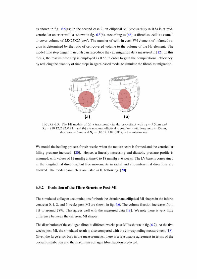
as shown in fig. 6.5(a); In the second case 2, an elliptical MI (eccentricity ≈ 0.8) is at mid-
ventricular anterior wall, as shown in fig. 6.5(b). According to [66], a fibroblast cell is assumed
to cover volume of 25X25X25 µm3. The number of cells in each FM element of infarcted re-
gion is determined by the ratio of cell-covered volume to the volume of the FE element. The
model time step bigger than 0.5h can reproduce the cell migration data measured in [12]. In this
thesis, the maxim time step is employed as 0.5h in order to gain the computational efficiency,
by reducing the quantity of time steps in agent-based model to simulate the fibroblast migration.
FIGURE 6.5: The FE models of (a) a transmural circular cryoinfarct with r0 ≈ 5.5mm andXc = (10.12,2.82,0.81), and (b) a transmural elliptical cryoinfarct (with long axix ≈ 15mm,
short axis ≈ 5mm and Xc = (10.12,2.82,0.81), in the anterior wall.
We model the healing process for six weeks when the mature scare is formed and the ventricular
filling pressure incrased [20]. Hence, a linearly-increasing end-diastolic pressure profile is
assumed, with values of 12 mmHg at time 0 to 18 mmHg at 6 weeks. The LV base is constrained
in the longitudinal direction, but free movements in radial and circumferential directions are
allowed. The model parameters are listed in II, following [20].
6.3.2 Evolution of the Fibre Structure Post-MI
The simulated collagen accumulations for both the circular and elliptical MI shapes in the infarct
centre at 0, 1, 2, and 5 weeks post-MI are shown in fig. 6.6. The volume fraction increases from
3% to around 28%. This agrees well with the measured data [18]. We note there is very little
difference between the different MI shapes.
The distribution of the collagen fibres at different weeks post-MI is shown in fig.(6.7). At the five
weeks post-MI, the simulated result is also compared with the corresponding measurement [18].
Given the large error bars in the measurements, there is a reasonable agreement in terms of the
overall distribution and the maximum collagen fibre fraction predicted.
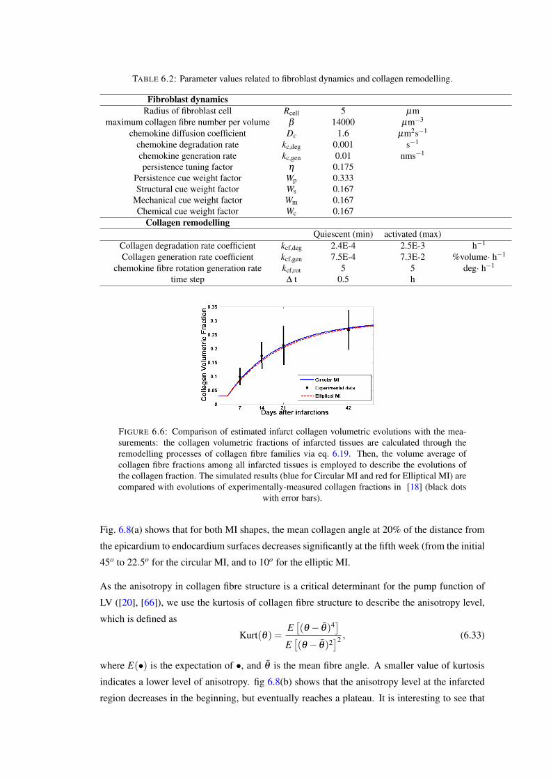
TABLE 6.2: Parameter values related to fibroblast dynamics and collagen remodelling.
Fibroblast dynamicsRadius of fibroblast cell Rcell 5 µm
maximum collagen fibre number per volume β 14000 µm−3
chemokine diffusion coefficient Dc 1.6 µm2s−1
chemokine degradation rate kc,deg 0.001 s−1
chemokine generation rate kc,gen 0.01 nms−1
persistence tuning factor η 0.175Persistence cue weight factor Wp 0.333Structural cue weight factor Ws 0.167
Mechanical cue weight factor Wm 0.167Chemical cue weight factor Wc 0.167
Collagen remodellingQuiescent (min) activated (max)
Collagen degradation rate coefficient kcf,deg 2.4E-4 2.5E-3 h−1
Collagen generation rate coefficient kcf,gen 7.5E-4 7.3E-2 %volume· h−1
chemokine fibre rotation generation rate kcf,rot 5 5 deg· h−1
time step ∆ t 0.5 h
FIGURE 6.6: Comparison of estimated infarct collagen volumetric evolutions with the mea-surements: the collagen volumetric fractions of infarcted tissues are calculated through theremodelling processes of collagen fibre families via eq. 6.19. Then, the volume average ofcollagen fibre fractions among all infarcted tissues is employed to describe the evolutions ofthe collagen fraction. The simulated results (blue for Circular MI and red for Elliptical MI) arecompared with evolutions of experimentally-measured collagen fractions in [18] (black dots
with error bars).
Fig. 6.8(a) shows that for both MI shapes, the mean collagen angle at 20% of the distance from
the epicardium to endocardium surfaces decreases significantly at the fifth week (from the initial
45o to 22.5o for the circular MI, and to 10o for the elliptic MI.
As the anisotropy in collagen fibre structure is a critical determinant for the pump function of
LV ([20], [66]), we use the kurtosis of collagen fibre structure to describe the anisotropy level,
which is defined as
Kurt(θ) =E[(θ − θ)4
]
E[(θ − θ)2
]2 , (6.33)
where E(•) is the expectation of •, and θ is the mean fibre angle. A smaller value of kurtosis
indicates a lower level of anisotropy. fig 6.8(b) shows that the anisotropy level at the infarcted
region decreases in the beginning, but eventually reaches a plateau. It is interesting to see that
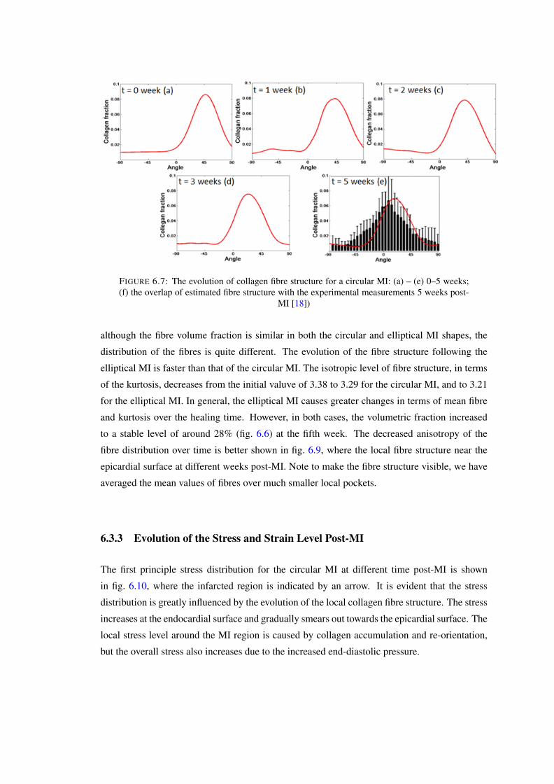
FIGURE 6.7: The evolution of collagen fibre structure for a circular MI: (a) – (e) 0–5 weeks;(f) the overlap of estimated fibre structure with the experimental measurements 5 weeks post-
MI [18])
although the fibre volume fraction is similar in both the circular and elliptical MI shapes, the
distribution of the fibres is quite different. The evolution of the fibre structure following the
elliptical MI is faster than that of the circular MI. The isotropic level of fibre structure, in terms
of the kurtosis, decreases from the initial valuve of 3.38 to 3.29 for the circular MI, and to 3.21
for the elliptical MI. In general, the elliptical MI causes greater changes in terms of mean fibre
and kurtosis over the healing time. However, in both cases, the volumetric fraction increased
to a stable level of around 28% (fig. 6.6) at the fifth week. The decreased anisotropy of the
fibre distribution over time is better shown in fig. 6.9, where the local fibre structure near the
epicardial surface at different weeks post-MI. Note to make the fibre structure visible, we have
averaged the mean values of fibres over much smaller local pockets.
6.3.3 Evolution of the Stress and Strain Level Post-MI
The first principle stress distribution for the circular MI at different time post-MI is shown
in fig. 6.10, where the infarcted region is indicated by an arrow. It is evident that the stress
distribution is greatly influenced by the evolution of the local collagen fibre structure. The stress
increases at the endocardial surface and gradually smears out towards the epicardial surface. The
local stress level around the MI region is caused by collagen accumulation and re-orientation,
but the overall stress also increases due to the increased end-diastolic pressure.
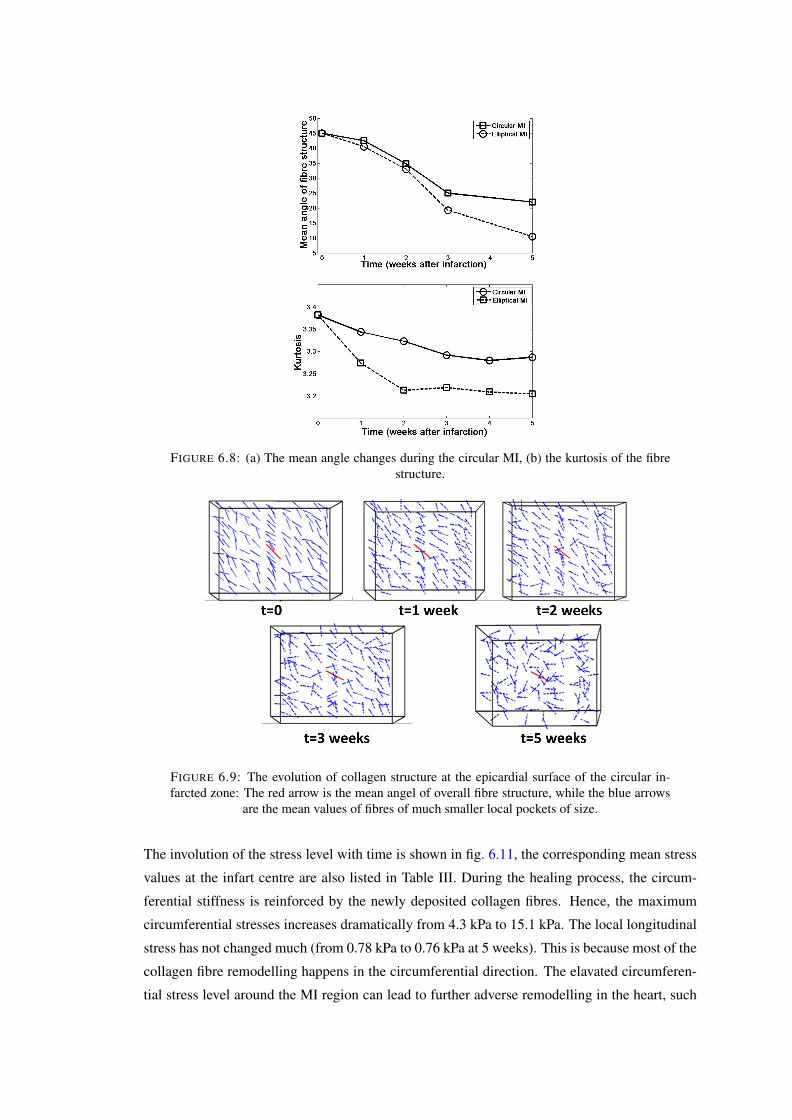
FIGURE 6.8: (a) The mean angle changes during the circular MI, (b) the kurtosis of the fibrestructure.
FIGURE 6.9: The evolution of collagen structure at the epicardial surface of the circular in-farcted zone: The red arrow is the mean angel of overall fibre structure, while the blue arrows
are the mean values of fibres of much smaller local pockets of size.
The involution of the stress level with time is shown in fig. 6.11, the corresponding mean stress
values at the infart centre are also listed in Table III. During the healing process, the circum-
ferential stiffness is reinforced by the newly deposited collagen fibres. Hence, the maximum
circumferential stresses increases dramatically from 4.3 kPa to 15.1 kPa. The local longitudinal
stress has not changed much (from 0.78 kPa to 0.76 kPa at 5 weeks). This is because most of the
collagen fibre remodelling happens in the circumferential direction. The elavated circumferen-
tial stress level around the MI region can lead to further adverse remodelling in the heart, such
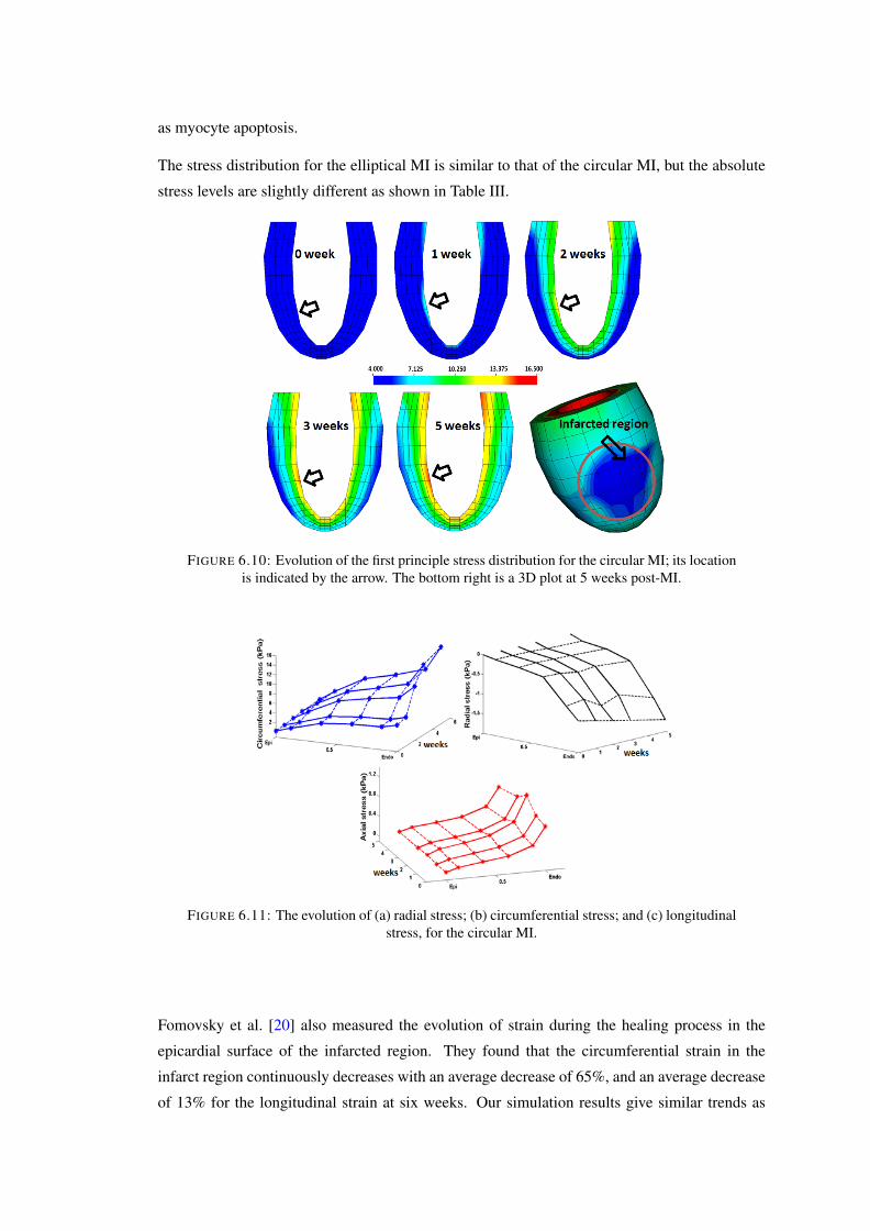
as myocyte apoptosis.
The stress distribution for the elliptical MI is similar to that of the circular MI, but the absolute
stress levels are slightly different as shown in Table III.
FIGURE 6.10: Evolution of the first principle stress distribution for the circular MI; its locationis indicated by the arrow. The bottom right is a 3D plot at 5 weeks post-MI.
FIGURE 6.11: The evolution of (a) radial stress; (b) circumferential stress; and (c) longitudinalstress, for the circular MI.
Fomovsky et al. [20] also measured the evolution of strain during the healing process in the
epicardial surface of the infarcted region. They found that the circumferential strain in the
infarct region continuously decreases with an average decrease of 65%, and an average decrease
of 13% for the longitudinal strain at six weeks. Our simulation results give similar trends as
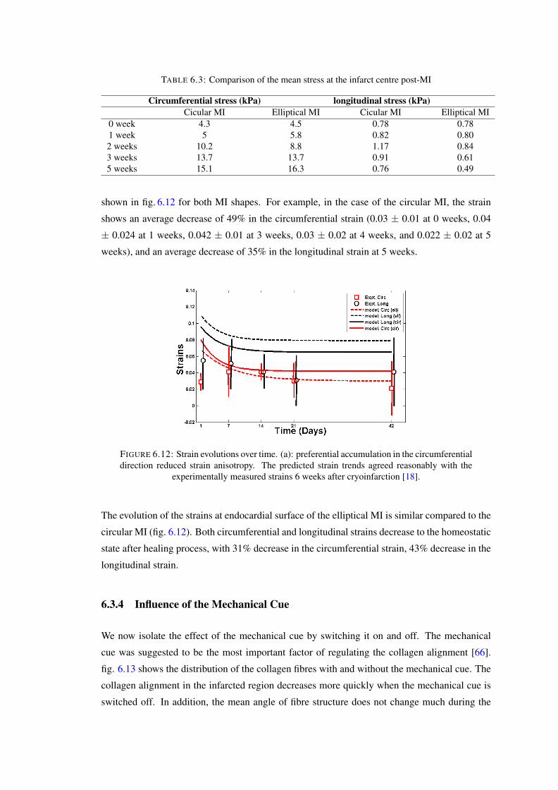
TABLE 6.3: Comparison of the mean stress at the infarct centre post-MI
Circumferential stress (kPa) longitudinal stress (kPa)Cicular MI Elliptical MI Cicular MI Elliptical MI
0 week 4.3 4.5 0.78 0.781 week 5 5.8 0.82 0.802 weeks 10.2 8.8 1.17 0.843 weeks 13.7 13.7 0.91 0.615 weeks 15.1 16.3 0.76 0.49
shown in fig. 6.12 for both MI shapes. For example, in the case of the circular MI, the strain
shows an average decrease of 49% in the circumferential strain (0.03 ± 0.01 at 0 weeks, 0.04
± 0.024 at 1 weeks, 0.042 ± 0.01 at 3 weeks, 0.03 ± 0.02 at 4 weeks, and 0.022 ± 0.02 at 5
weeks), and an average decrease of 35% in the longitudinal strain at 5 weeks.
FIGURE 6.12: Strain evolutions over time. (a): preferential accumulation in the circumferentialdirection reduced strain anisotropy. The predicted strain trends agreed reasonably with the
experimentally measured strains 6 weeks after cryoinfarction [18].
The evolution of the strains at endocardial surface of the elliptical MI is similar compared to the
circular MI (fig. 6.12). Both circumferential and longitudinal strains decrease to the homeostatic
state after healing process, with 31% decrease in the circumferential strain, 43% decrease in the
longitudinal strain.
6.3.4 Influence of the Mechanical Cue
We now isolate the effect of the mechanical cue by switching it on and off. The mechanical
cue was suggested to be the most important factor of regulating the collagen alignment [66].
fig. 6.13 shows the distribution of the collagen fibres with and without the mechanical cue. The
collagen alignment in the infarcted region decreases more quickly when the mechanical cue is
switched off. In addition, the mean angle of fibre structure does not change much during the
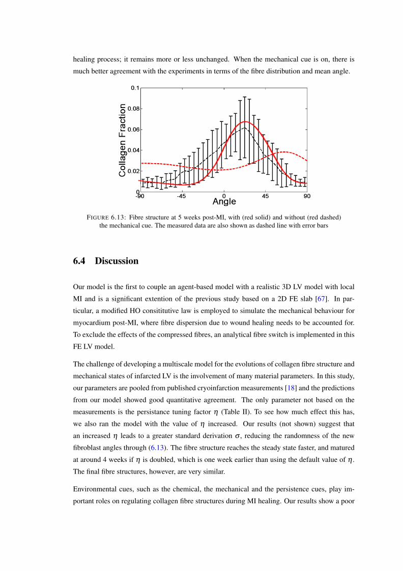
healing process; it remains more or less unchanged. When the mechanical cue is on, there is
much better agreement with the experiments in terms of the fibre distribution and mean angle.
FIGURE 6.13: Fibre structure at 5 weeks post-MI, with (red solid) and without (red dashed)the mechanical cue. The measured data are also shown as dashed line with error bars
6.4 Discussion
Our model is the first to couple an agent-based model with a realistic 3D LV model with local
MI and is a significant extention of the previous study based on a 2D FE slab [67]. In par-
ticular, a modified HO consititutive law is employed to simulate the mechanical behaviour for
myocardium post-MI, where fibre dispersion due to wound healing needs to be accounted for.
To exclude the effects of the compressed fibres, an analytical fibre switch is implemented in this
FE LV model.
The challenge of developing a multiscale model for the evolutions of collagen fibre structure and
mechanical states of infarcted LV is the involvement of many material parameters. In this study,
our parameters are pooled from published cryoinfarction measurements [18] and the predictions
from our model showed good quantitative agreement. The only parameter not based on the
measurements is the persistance tuning factor η (Table II). To see how much effect this has,
we also ran the model with the value of η increased. Our results (not shown) suggest that
an increased η leads to a greater standard derivation σ , reducing the randomness of the new
fibroblast angles through (6.13). The fibre structure reaches the steady state faster, and matured
at around 4 weeks if η is doubled, which is one week earlier than using the default value of η .
The final fibre structures, however, are very similar.
Environmental cues, such as the chemical, the mechanical and the persistence cues, play im-
portant roles on regulating collagen fibre structures during MI healing. Our results show a poor
agreement with measurements if the mechanical cue is switched off. McDougall et al. sug-
gested that the distribution of the chemical gradient established by the chemokines generated
around dermal wound, determines patterns of local collagen alignment [53]. In our simulations,
different chemokine distributions are realised through the MI shapes; the chemokine field is
mostly flat inside the infarction, but with a sudden drop near the infarct border. The influences
of chemical gradient are greater in the region near infarcted border. Therefore, the mean angle
and kurtosis of the fibre distribution for different infarct shapes are different. Our simulations
are also supported by the observations in [66].
Finally, we mention the limitations of this study. Firstly, the transmural fibroblast migration
is not considered. Secondly, our model only consider the diastolic dynamics without active
contraction. Therefore the mechanical cue is simplified. Furthermore, no transient chemokine
concentration is included. Finally, we understand that myocardial infarction in the human heart
may have different biological processes and parameters compared to cryoinfarction in the rat
heart. Estimation of these parameters for paticent-specific human hearts post-MI, therefore,
remains a daunting task.
6.5 Conclusion
We have developed a multiscale MI model by coupling an agent-based model for collagen re-
modelling to a three-dimensional LV model in diastole. To describe the remodelled material
properties of myocardium in the infarted region, a collagen fibre tension-compression ‘switch’
is incorporated in the FE LV model for the first time. The time-dependent model also captures
the interaction and information exchange processes between the mechanical behaviour and col-
lagen tissue remodelling guided by various external cues. The model results show the similar
trends in collagen cumulation and collagen alignment during the infarct healing for five weeks.
The shapes and the locations of infarctions could affect the local collagen accumulation and the
LV dynamics. For example, the mean angle of fibre structure decreases from about 45o to 22.5o
at near the endocardial surface for the circle infarction, but decreases less in the elliptic infarc-
tion. Stresses are affected for both the circle and the ellipse infarctions. The reduction of the
circumferential strains at five weeks post-MI agrees well with the experimental observations.
With further development, we expect that this multiscale approach could provide useful insights
in clinical practices for MI patient management.
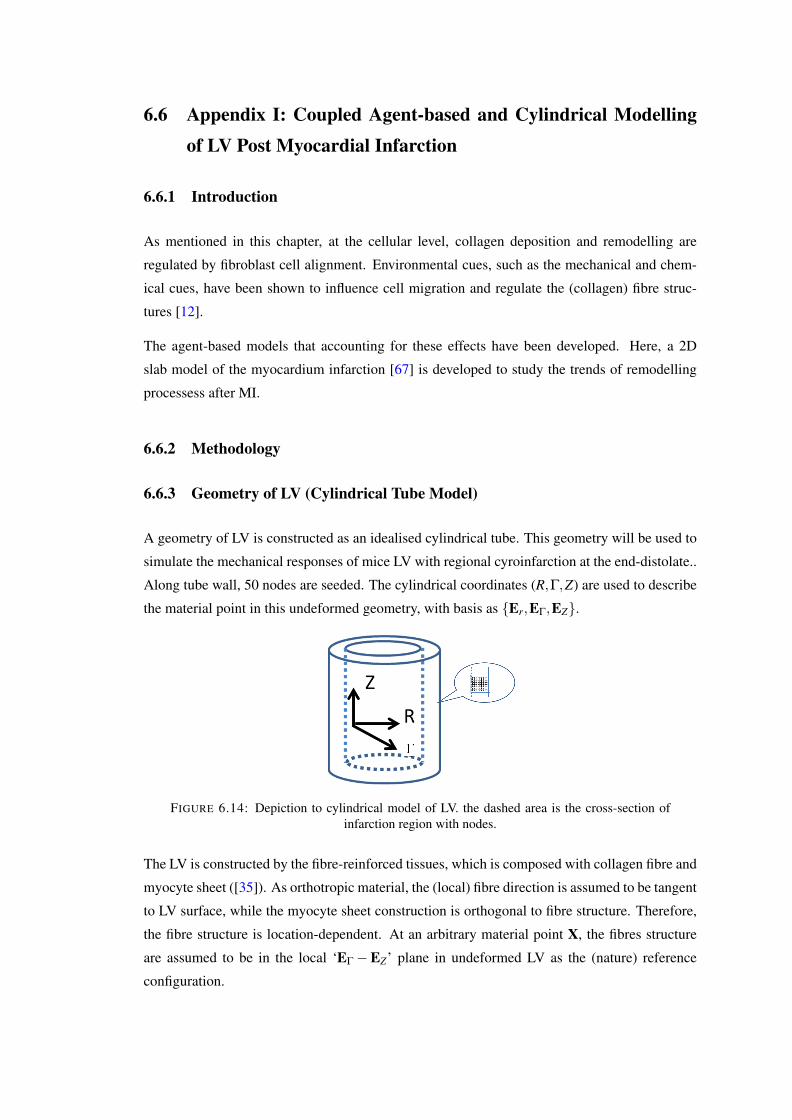
6.6 Appendix I: Coupled Agent-based and Cylindrical Modellingof LV Post Myocardial Infarction
6.6.1 Introduction
As mentioned in this chapter, at the cellular level, collagen deposition and remodelling are
regulated by fibroblast cell alignment. Environmental cues, such as the mechanical and chem-
ical cues, have been shown to influence cell migration and regulate the (collagen) fibre struc-
tures [12].
The agent-based models that accounting for these effects have been developed. Here, a 2D
slab model of the myocardium infarction [67] is developed to study the trends of remodelling
processess after MI.
6.6.2 Methodology
6.6.3 Geometry of LV (Cylindrical Tube Model)
A geometry of LV is constructed as an idealised cylindrical tube. This geometry will be used to
simulate the mechanical responses of mice LV with regional cyroinfarction at the end-distolate..
Along tube wall, 50 nodes are seeded. The cylindrical coordinates (R,Γ,Z) are used to describe
the material point in this undeformed geometry, with basis as Er,EΓ,EZ.
FIGURE 6.14: Depiction to cylindrical model of LV. the dashed area is the cross-section ofinfarction region with nodes.
The LV is constructed by the fibre-reinforced tissues, which is composed with collagen fibre and
myocyte sheet ([35]). As orthotropic material, the (local) fibre direction is assumed to be tangent
to LV surface, while the myocyte sheet construction is orthogonal to fibre structure. Therefore,
the fibre structure is location-dependent. At an arbitrary material point X, the fibres structure
are assumed to be in the local ‘EΓ−EZ’ plane in undeformed LV as the (nature) reference
configuration.
The infarction is developed respect to the infarction center zone, which is defined as
Ro ≥ R≥ Ri, 2π ≥ Γ≥ 0, L≥ Z ≥ 0
where Ri and Ro are the outer and inner radius of LV cylindrical tube.
6.6.3.1 Agent-based Model
6.6.3.2 MI Healing and Chemokine Concentration
The general form of chemokine concentration is given in eq. (6.2), as well as the boundary
conditions in eqs. (6.3) and (6.4). In this simplified model, the chemokine concentration is
assumed to only depend on the distance along z-axis from the infarct center. Therefore, the
chemokine concentration could be rewritten in cylindrical coordinates R,Γ,Z as
Dc52 C(Z) =
kc,degC(Z)− kc,gen Z < Z0,
kc,degC(Z) Z ≥ Z0,(6.34)
where C(Z) is the concentration equation in cylindrical coordinate (C(Z) =C(X−Xc)), Z0 is at
the infarct boundary.
The boundary conditions (eqs. (6.3) and (6.4)) are rewritten as
(dCdZ |Z=Z0
)+ = (dCdZ |Z=Z0
)− if Z = Z0,
C |Z=Z0)+ = (C |Z=Z0)
− if Z = Z0,
C = 0 if Z = ∞,
dCdZ = 0, at Z = 0.
(6.35)
The chemokine equation could be obtained from eq. (6.34) and (6.35) as (fig. 6.15)
C(Z) = a1exp(a2Z)+a1exp(−a2Z)+a0 Z < Z0, (6.36)
where a0 =kc,genkc,deg
, a2 =√
kc,degDc
, a1 =− a02exp(a2Z0)
6.6.3.3 Fibroblast Movement Regulated by Environmental Cues
The fibroblast migrations respond to local environmental cues [19]. Here, the fibroblasts are
modelled as rigid discs. The environmental cues for individual cell are defined as: The fi-
broblast migration are regulated by internal and external environmental cues, such as chemical,
mechanical, persistent and structural cues ([12], [19], [66]).
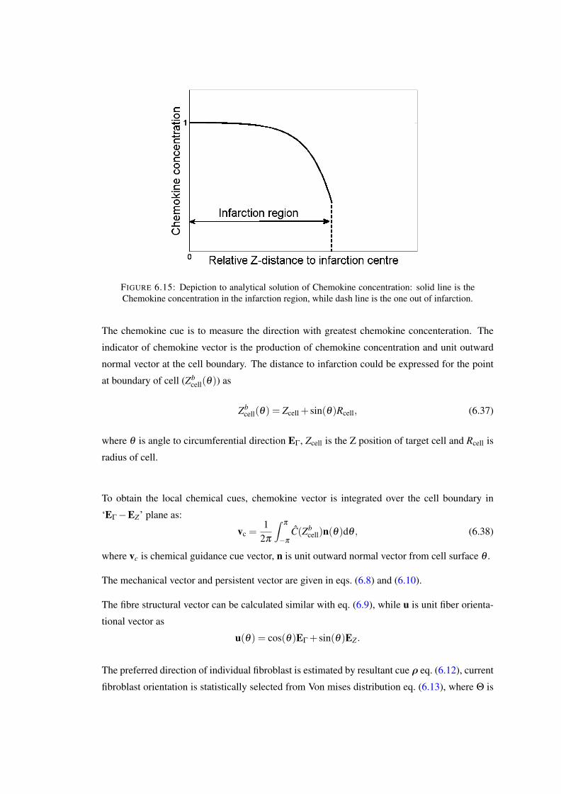
FIGURE 6.15: Depiction to analytical solution of Chemokine concentration: solid line is theChemokine concentration in the infarction region, while dash line is the one out of infarction.
The chemokine cue is to measure the direction with greatest chemokine concenteration. The
indicator of chemokine vector is the production of chemokine concentration and unit outward
normal vector at the cell boundary. The distance to infarction could be expressed for the point
at boundary of cell (Zbcell(θ)) as
Zbcell(θ) = Zcell + sin(θ)Rcell, (6.37)
where θ is angle to circumferential direction EΓ, Zcell is the Z position of target cell and Rcell is
radius of cell.
To obtain the local chemical cues, chemokine vector is integrated over the cell boundary in
‘EΓ−EZ’ plane as:
vc =1
2π
∫π
−π
C(Zbcell)n(θ)dθ , (6.38)
where vc is chemical guidance cue vector, n is unit outward normal vector from cell surface θ .
The mechanical vector and persistent vector are given in eqs. (6.8) and (6.10).
The fibre structural vector can be calculated similar with eq. (6.9), while u is unit fiber orienta-
tional vector as
u(θ) = cos(θ)EΓ + sin(θ)EZ.
The preferred direction of individual fibroblast is estimated by resultant cue ρ eq. (6.12), current
fibroblast orientation is statistically selected from Von mises distribution eq. (6.13), where Θ is
the angle of a single fibroblast cell, Θ is the mean angle of the fibroblast resultant vector ρ in
local ‘EΓ−EZ’.
In this reduced agent-based model, the movement of fibroblast is ignored, while it only considers
the rotation of fibroblast in ‘EΓ−EZ’ plain.
Remodeling of Fibre Structure by Fibroblast CellAfter the fibroblast orientation is statistically determined from eq. (6.13), the structure of the
collagen fibres is updated, represented by eqs. (6.15) and (6.16).
6.6.3.4 Upscaling the Fibre Structure from Fibre Level to Tissue Level
In the tissue level, the fibre structure can be described by the fibre volumetric fraction (Φcf) and
fibre orientation density function (ϕt(θ)) at time t, which parameters are updated by eqs. (6.19)
and (6.20).
6.6.4 Basic Kinematics of Tube Model
Consider LV of heart as an incompressible thick-walled cylindrical tube subjected to external
loads. Then, in cylindrical polar coordinates R,Γ,Z, the geometry of heart tube is defined by
Ro ≥ R≥ Ri, 2π ≥ Γ≥ 0, L≥ Z ≥ 0
where L is the length of tube.
After applying external loads (heart pressure), in term of (r,γ,z), the geometry of current con-
figuration is given by
ro ≥ r ≥ ri, 2π ≥ γ ≥ 0, l ≥ z≥ 0
where ri, ro and l are inner, outer radii and length of deformed tube, respectively.
The isochoric deformation from the undeformed configuration to current configuration is written
as
x = rer + zez, (6.39)
Material incompressibility gives
r =
√R2−R2
iλz
+ r2i , γ = Γ, z = λzZ, (6.40)
where λz = l/L is the constant axial stretch.
The deformation gradient, denoted as F, is given by
F =∂x∂X
= λ1er⊗ER +λ2eγ ⊗EΓ +λzez⊗EZ, (6.41)
where
λ1 =R
rλz, λ2 =
rR
(6.42)
For the tube model, the equilibrium equation5σ = 0 is reduced to
dσrr
dr+
σrr−σγγ
r= 0, (6.43)
With help of pressure boundary condition (P =−σrr|r=ri), on integration equation (6.43) gives
P =∫ ro
ri
σγγ −σrr
rdr. (6.44)
This equation will be used to determine the mechanical response of LV to heart pressure, with
help of constitutive laws for passive heart tissues.
6.6.5 Constitutive Laws for LV Tissues
6.6.5.1 Modified HO Model with Fibre Orientation Density Function
The modified HO model is used to describe the constitutive law for heart tissues (eqs. (6.24) -
(6.25)).
For the healthy myocardium, the fibre dispersion could be experimentally fitted with a Von mises
distribution [38, 70] or a wrapped normal distribution [66]. In this paper, we use the π-periodic
Von mises distribution to describe the fibre orientation density function ϕ0 for healthy tissue.
ϕ0(θ) =eσ0cos(θ−θ)
I0(σ0)
where σ0 is the initial concentration parameter, fitted from experimental observation [66], θ is
the mean angle of collagen fibre structure. I0(σ0) is the modified Bessel’s function of first kind
of order zero [70] as
I0(σ0) =1π
∫π
0exp(σ cosθ)dθ .
The in vitro experimental measurement shows the mean angle of fibre rotates transmurally
across the heart wall from π/3 at the endocardial surface to −π/3 at the epicardial surface.
Here, the myocardium fibre generation algorithm ( [89, 95]) is adopted to simulate the local
fibre mean angle. For an arbitrary material point X of heart tube, the normalized thickness
parameter d could be determined by two intramural distances as
d =RX −Ri
Ro−Ri(6.45)
The local mean angle of fibre structure could be simulated as
θ = θmax(1−2d)
where θmax is the maximum fibre angle on the endocardial surface, as π
3 in this paper.
6.6.5.2 Fibre Switch to Exclude the Compressed Fibre
In the computation of mechanical behavior of myocardium, the undeformed fibre structure is
assumed to distribute in the ‘EΓ−EZ’ plane. The compressed collagen fibres should be exclued
from the mechanical contributions, which requires It requires to solving the inequation of fibre
invariance
I4 > 1 (6.46)
where I4 is the fibre invariant; with unit basis ER,EΓ,EZ, the right Cauchy–Green tensor
(C = FT F) is given with help of eq. (6.41) as
C = λ21 ER⊗ER +λ
22 EΓ⊗EΓ +λ
2z EZ⊗EZ. (6.47)
Substituting eq. (6.47) into eq. (6.46), it gives
I4 = λ22 cos2
θ +λ2z sin2
θ > 1, (6.48)
By solving inequality (6.46), the solution is given as:
Case 1:
if λ2 > 1, θ ∈ Σ = (−π
2 ,π
2 ).
Case 2:
if λ2 < 1,
θ ∈ Σ = (
√arctan
1−λ 22
λ 2z −1
,π
2)∪ (−π
2,−√
arctan1−λ 2
2λ 2
z −1). (6.49)
Then, the angel range Σ will be used to describe the stretched collagen fibres in (6.50)
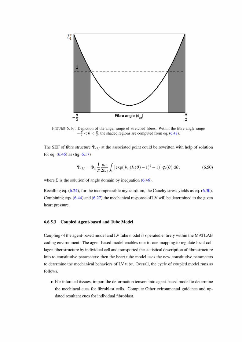
FIGURE 6.16: Depiction of the angel range of stretched fibres: Within the fibre angle range−π
2 < θ < π
2 , the shaded regions are computed from eq. (6.48).
The SEF of fibre structure Ψcf,t at the associated point could be rewritten with help of solution
for eq. (6.46) as (fig. 6.17)
Ψcf,t = Φcf1π
acf
2bcf
∫
Σ
[exp( bcf(I4(θ)−1)2−1)
]ϕt(θ) dθ , (6.50)
where Σ is the solution of angle domain by inequation (6.46).
Recalling eq. (6.24), for the incompressible myocardium, the Cauchy stress yields as eq. (6.30).
Combining eqs. (6.44) and (6.27),the mechanical response of LV will be determined to the given
heart pressure.
6.6.5.3 Coupled Agent-based and Tube Model
Coupling of the agent-based model and LV tube model is operated entirely within the MATLAB
coding environment. The agent-based model enables one-to-one mapping to regulate local col-
lagen fiber structure by individual cell and transported the statistical description of fibre structure
into to constitutive parameters; then the heart tube model uses the new constitutive parameters
to determine the mechanical behaviors of LV tube. Overall, the cycle of coupled model runs as
follows.
• For infarcted tissues, import the deformation tensors into agent-based model to determine
the mechincal cues for fibroblast cells. Compute Other evironmental guidance and up-
dated resultant cues for individual fibroblast.
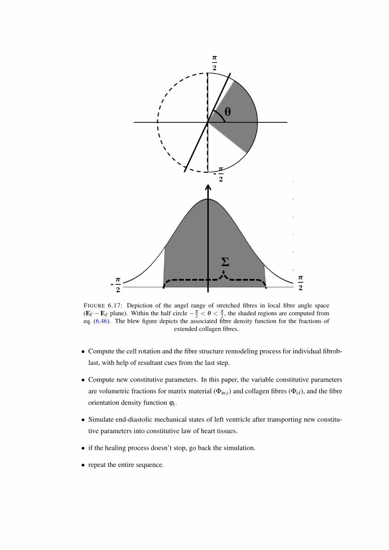
FIGURE 6.17: Depiction of the angel range of stretched fibres in local fibre angle space(EΓ−EZ plane). Within the half circle −π
2 < θ < π
2 , the shaded regions are computed fromeq. (6.46). The blew figure depicts the associated fibre density function for the fractions of
extended collagen fibres.
• Compute the cell rotation and the fibre structure remodeling process for individual fibrob-
last, with help of resultant cues from the last step.
• Compute new constitutive parameters. In this paper, the variable constitutive parameters
are volumetric fractions for matrix material (Φm,t) and collagen fibres (Φcf), and the fibre
orientation density function ϕt .
• Simulate end-diastolic mechanical states of left ventricle after transporting new constitu-
tive parameters into constitutive law of heart tissues.
• if the healing process doesn’t stop, go back the simulation.
• repeat the entire sequence.
6.6.5.4 MI Healing Case Studies
The evolutions of fibre structure and mechanical behaviors of LV have been experimentally in-
vestigated by Holmes [20]. In [20], the Cyroinfarctions are created by sewing sonomicrometer
crystals into tissues of the epicardial surface of rats’ LV. Then, after weeks, the hearts are har-
vested to study the local strain and the fibre structures of infarcted tissues, which information
are collected from the tissues at surface of infarction zone.
In this chapter, it will simulate the remodeling processes of infarcted LV. The constant end-
diastole pressure 1.6 (Kpa) is applied on the inner surface. After running the coupled model,
the evolutions of collagen volumetric fraction, strains, and stress are simulated over 6 weeks
after infarction. To show the influences of the healing process at different location from LV
infarction, it investigates the evolutions of stresses and fibre structure for tissues from different
locations (fig. 6.19), with different infarction level: (1) the center of infarction, this position is
at the center of infarction under highest chemokine effects (Z = 0); (2) middle of the infarction,
this position is at the middle of infarction center to the infarction edge (Z = L2 ); (3) edge of
infarction, this is the remote region for infarction (Z = L).
6.6.6 Results
After introducing a regional infarction to the coupled agent-based and elastic tube model, the
change of the collagen structure and mechanical behaviors of LV are simulated.
6.6.6.1 Results for Tissues at Center of Infarction Region
The impacts of infarction occur 3 days after the coronary ligation, while the healing process
of heart will start simultaneously with same lag. In this paper, the lengths of collagen fibres
are assumed to be constant and stable. Then, the volumetric fraction evolution in infarct my-
ocardium tissue could be directly estimated by the quantitative changes of the total collagen
numbers (eq. (6.19)). The value ranges of collagen deposition (kcf,deg) and generation (kcf,gen)
rates (table 6.2) are fitted from the published experimental data ([12]) by Holmes [66]. The col-
lagen accumulations are measured at 1, 2, 3, 6 weeks after coronary ligation [18] (from 0.028
to around 0.3), which match well with our calculation (fig. 6.18). Along with the changes of
the fibre structure, the mean angle of fibre is also changed. At the epi surface, the mean angle
decreases from 60o at 0 week to 20o at six weeks (fig. 6.18b).
The fibre structure is also measured by the collagen fraction for fibre angles. As shown in
fig. 6.19, the anisotropic level of fibre structure is decreased, with the decreasing fibre angle

FIGURE 6.18: Estimated infarct collagen volumetric and mean angle evolution at epi sur-face of infarction heart (Center): Left, the collagen volumetric accumulations are measured byFomevsky [18] (black dots with error bars), comparing with the estimation by coupled model
(blue line); Right, the changes of mean angle during healing process
concentration. The results suggest that the fibre structure will be more isotropic at the infarc-
tion, which phenomenon is also experimentally observed [66].
FIGURE 6.19: The evolution of collagen fibre structure: (a) – (e) 0–5 weeks.
At the infarct zone, collagen accumulation caused stiffening of the infarct area. However,
the matrix material is volumetrically replaced by the collagen fibres. In contrast to the fibre-
reinforcement along fibre directions, the stiffness is negligibly decreased along transmural di-
rection. The stress distributions suggest that the radial stress doesn’t change too much during the
development of infarction at the infarction center (fig. 6.20a). The max circumferential stresses
(σγγ ) are continuously increased (3.8 Kpa at 0 week to 5.3 Kpa at 6 weeks at endo surface,
fig. 6.20b ). The local longitudinal stress (σzz) is decreased (2.3 Kpa at 0 week to 0.4 Kpa at 6
weeks at the endo surface fig. 6.20c ). Obviously, the concentration of first principal stress, as
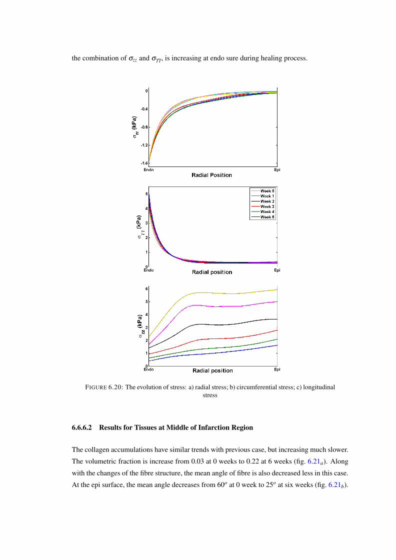
the combination of σzz and σγγ , is increasing at endo sure during healing process.
FIGURE 6.20: The evolution of stress: a) radial stress; b) circumferential stress; c) longitudinalstress
6.6.6.2 Results for Tissues at Middle of Infarction Region
The collagen accumulations have similar trends with previous case, but increasing much slower.
The volumetric fraction is increase from 0.03 at 0 weeks to 0.22 at 6 weeks (fig. 6.21a). Along
with the changes of the fibre structure, the mean angle of fibre is also decreased less in this case.
At the epi surface, the mean angle decreases from 60o at 0 week to 25o at six weeks (fig. 6.21b).
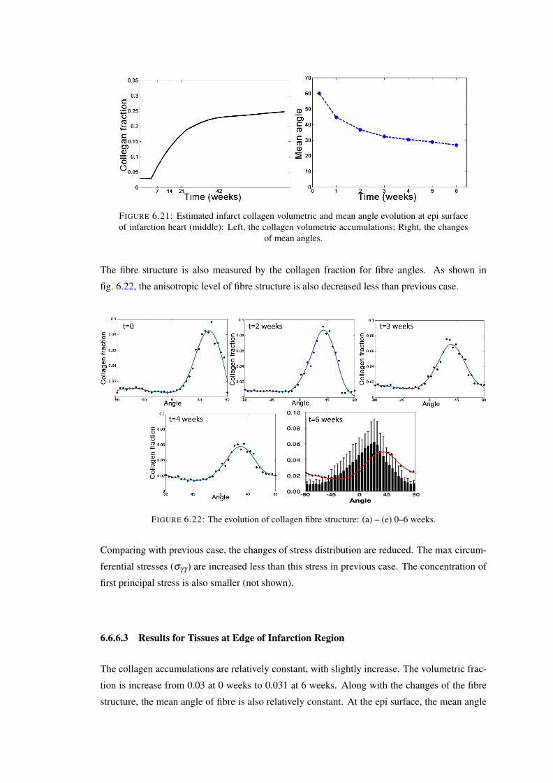
FIGURE 6.21: Estimated infarct collagen volumetric and mean angle evolution at epi surfaceof infarction heart (middle): Left, the collagen volumetric accumulations; Right, the changes
of mean angles.
The fibre structure is also measured by the collagen fraction for fibre angles. As shown in
fig. 6.22, the anisotropic level of fibre structure is also decreased less than previous case.
FIGURE 6.22: The evolution of collagen fibre structure: (a) – (e) 0–6 weeks.
Comparing with previous case, the changes of stress distribution are reduced. The max circum-
ferential stresses (σγγ ) are increased less than this stress in previous case. The concentration of
first principal stress is also smaller (not shown).
6.6.6.3 Results for Tissues at Edge of Infarction Region
The collagen accumulations are relatively constant, with slightly increase. The volumetric frac-
tion is increase from 0.03 at 0 weeks to 0.031 at 6 weeks. Along with the changes of the fibre
structure, the mean angle of fibre is also relatively constant. At the epi surface, the mean angle
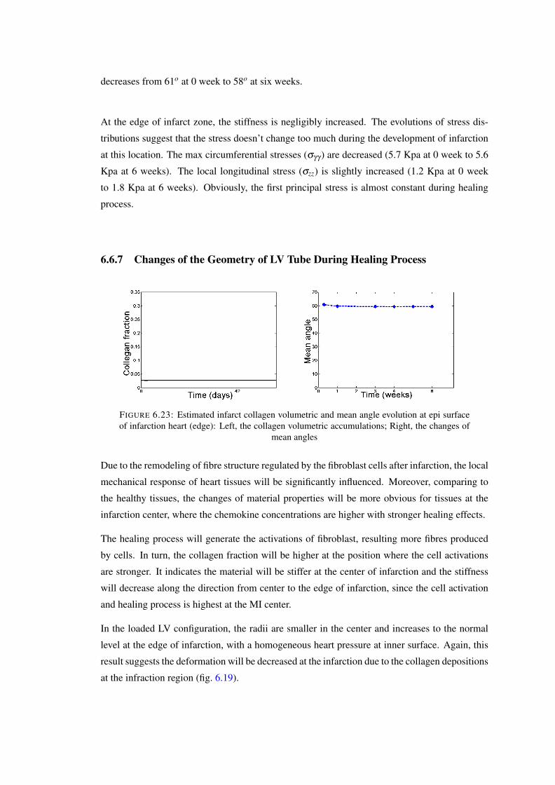
decreases from 61o at 0 week to 58o at six weeks.
At the edge of infarct zone, the stiffness is negligibly increased. The evolutions of stress dis-
tributions suggest that the stress doesn’t change too much during the development of infarction
at this location. The max circumferential stresses (σγγ ) are decreased (5.7 Kpa at 0 week to 5.6
Kpa at 6 weeks). The local longitudinal stress (σzz) is slightly increased (1.2 Kpa at 0 week
to 1.8 Kpa at 6 weeks). Obviously, the first principal stress is almost constant during healing
process.
6.6.7 Changes of the Geometry of LV Tube During Healing Process
FIGURE 6.23: Estimated infarct collagen volumetric and mean angle evolution at epi surfaceof infarction heart (edge): Left, the collagen volumetric accumulations; Right, the changes of
mean angles
Due to the remodeling of fibre structure regulated by the fibroblast cells after infarction, the local
mechanical response of heart tissues will be significantly influenced. Moreover, comparing to
the healthy tissues, the changes of material properties will be more obvious for tissues at the
infarction center, where the chemokine concentrations are higher with stronger healing effects.
The healing process will generate the activations of fibroblast, resulting more fibres produced
by cells. In turn, the collagen fraction will be higher at the position where the cell activations
are stronger. It indicates the material will be stiffer at the center of infarction and the stiffness
will decrease along the direction from center to the edge of infarction, since the cell activation
and healing process is highest at the MI center.
In the loaded LV configuration, the radii are smaller in the center and increases to the normal
level at the edge of infarction, with a homogeneous heart pressure at inner surface. Again, this
result suggests the deformation will be decreased at the infarction due to the collagen depositions
at the infraction region (fig. 6.19).
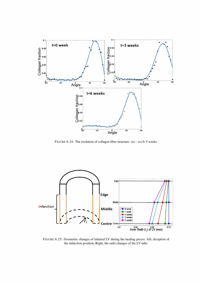
FIGURE 6.24: The evolution of collagen fibre structure: (a) – (e) 0–5 weeks.
FIGURE 6.25: Geometric changes of infarted LV during the healing prcess: left, deciption ofthe infarction position; Right, the radii changes of the LV tube.
6.6.8 Summary
A multiscale model, by coupling an agent-based model with a simplified left ventricle tube,
is developed. To simulate the appropriate material properties for myocardium, a fibre tension-
compression ’switch’ is employed as well. The time-dependent model also captures the inter-
action and information exchange process between mechanical behaviour and collagen tissue
remodelling guided by various external cues. The predicted results show the collagen cumula-
tions differ with the location in infraction region. By studying locations of infarctions, it shows
the location affects the mechanical behaviors of total LV and the fibre structure.
For fibre structure, the observed fibre changes decrease along distance to infarction center during
MI process. The fibre volumetric fraction increases from 0.03 to around 0.3 at the infarction
center, while it only increases from 0.03 to 0.031. For mean angle of fibre structure, it decreases
from about 60o 20o at endosurface at infarction center, while only small change of mean angle is
shown for fibre structure at infarction edge. Therefore, the trends of evolutions of fibre structures
are significantly influenced by the distance to infraction center.
For stress state, in this simplified tube model, the trends of stress distributions are similar during
MI process at different heart locations. However, the stress concentration is obviously changes.
At infarction center, the stress concentration is obviously increased at endosurface during MI,
while it’s almost constant for stress evolution at infarction center. Moreover, the higher fi-
bre fraction indicates tissues are stiffer at infarction center, which gives the smaller radius of
heart tube. During MI process, after applying passive heart pressure, the shape of heart tube is
changed, while the radius of cylinder is reduced along LV axis.
6.7 Appendix II: Tangent Stiffness
If we want to solve the LV dynamics, the tangent stiffness (4th order) matrix C is needed in
FEAP software. We start from the moduli matrix C for the second Piola-Krirchoff stress P at the
reference configuration, then push forwards the moduli matrix C into the current configuration.
if C = 2∂P∂C
then C= J−1FFFFC , (6.51)
or Ci jkl = J−1FiIFjJFkKFlLCIJKL.
The myocardial constitutive law consists of the matrix Ψm(C), collagen fibre Ψcf(I4) and pure
volumetric penalty Ψv(J) to ensure the material incompressibility, that is
Ψ = Ψv(J)+ Ψm(C)+ Ψcf(I4), (6.52)
in which Ψ is a purely isochoric contribution. The volumetric penalty term is
Ψv =k2(J−1)2,
the term for the matrix material is
Ψm = Φm,ta2b
[exp b(I1−3)−1] ,
and the term of the collagen structure is:
Ψcf,t = Φcf,t1π
acf
2bcf
∫ [exp bcf(I4(θ)−1)2−1
]ϕt(θ) dθ ,
in which I1(= C : I) is the modified first invariance, I4(= fT0 ·Cf0) is the modified fibre invariance.
The second Piola-Krirchoff stress is
P = 2∂Ψ
∂C= 2
∂ (Ψv(J)+ Ψm(C)+ Ψcf(C))
∂C,
then the stiffness matrix in eq. (6.51) becomes
C = 2∂P∂C
= 4(∂ 2Ψv
∂C2 +∂ 2Ψm
∂C2 +∂ 2Ψcf
∂C2 ). (6.53)
Finally the Cauchy stress is expressed as
σ = k(J−1)I+Φm,t a exp[b(I1−3)]devb
+1π
Φcf,t
∫
Σ
2af(I4−1)exp[bf(I4−1)2]ϕt(θ) dev(f⊗ f)dθ ,(6.54)
in which the operator dev(•) is
dev(•) = (•)− 13[(•) : I]I
The tangent moduli C can be deduced for each individual contributions, respectively.
6.7.1 Second Order Derivation for Penalty Function
6.7.1.1 First Order Derivation ( ∂Ψv∂C )
By definition, it gives∂Ψv
∂C=
∂Ψv
∂J∂J∂C
=k2(J2− J)C−1, (6.55)
where ∂J∂C = 1
2 JC−1.
6.7.1.2 Second Order Derivation ( ∂ 2Ψv∂C2 )
With help of eq. (6.55), it gives
∂ 2Ψv
∂C2 =(∂ k
2(J2− J)C−1)
∂C
=k4
(2J2− J) ·C−1⊗C−1− (J2− J) · (C−1
(IK)⊗C−1(JL)+C−1
(IL)⊗C−1(JK))
,
(6.56)
where the orders of subscripts are ’IJKL’ for a normal 4th order tensor, for example, C−1(IL)⊗
C−1(JK) =C−1
IL C−1JK EI⊗EL⊗EJ⊗EK .
6.7.2 Second Order Derivation for SEF of Matrix
6.7.2.1 First Order Derivation ( ∂ Ψm∂C )
By Ψm, it gives
∂ Ψm
∂C= Φm,t
a2
exp(b(I1−3))∂ I1
∂C= Φm,t
a2
exp(b(I1−3))[−1
3I1C−1 + J−2/3I
], (6.57)
where ∂ I1∂C =−1
3 I1C−1 + J−2/3I.
6.7.2.2 Second order derivation ( ∂ 2Ψm∂C2 )
With help of eq. (6.57), we have
∂ 2Ψm
∂C2 = Φm,t∂a
2 exp(b(I1−3))[−1
3 I1C−1 + J−2/3I]
∂C
= Φm,taγ
2(b[−1
3I1C−1 + J−2/3I
]⊗[−1
3I1C−1 + J−2/3I
]
− 13
C−1⊗ (−13
I1C−1 + J−2/3I)+16
I1(C−1(IK)⊗C−1
(JL)+C−1(IL)⊗C−1
(JK))
− 13
J−2/3I⊗C−1),
(6.58)
where γ = exp(b(I1−3)).
6.7.3 Second Order Derivation for SEF of Collagen Structure
6.7.3.1 First Order Derivation ∂ Ψcf∂C
By Ψ f , it gives
∂ Ψ f
∂C=
Φcf,t
π
∫ϕ Ω
′(I4) ·∂ I4
∂Cdθ =
Φcf,t
π
∫ϕΩ′(I4)
[−1
3I4C−1 + J−2/3f0⊗ f0
]dθ , (6.59)
where ∂ I4∂C = −1
3 I4C−1 + J−2/3f0⊗ f0, and Ω(I4) =acf
2bcfexp (bcf(I4− 1)2− 1), Ω′(I4) =
∂Ω
∂ I4=
acf(I4−1)(exp bcf(I4−1)2)
6.7.3.2 Second Order Derivation ( ∂ 2Ψcf∂C2 )
With the help of eq. (6.59), it gives
∂ 2Ψcf
∂C2 =∂ (
Φcf,tπ
∫ϕΩ′(I4)
[−1
3 I4C−1 + J−2/3f0⊗ f0]
dθ)
∂C
=Φcf,t
π
∫ϕΩ′′[−1
3I4C−1 + J−2/3f0⊗ f0
]⊗[−1
3I4C−1 + J−2/3f0⊗ f0
]dθ
+Φcf,t
π
∫ϕΩ′ (−1
3C−1⊗ (−1
3I4C−1 + J−2/3f0⊗ f0)+
16
I4(C−1(IK)⊗C−1
(JL)+C−1(IL)⊗C−1
(JK))
− 13
J−2/3(f0⊗ f0)⊗C−1) dθ ,
(6.60)
where Ω′′(I4) = acf(exp bcf(I4−1)2)(1+2bcf(I4−1)2)
6.7.4 Tangent moduli C
With helps of eq. (6.56), (6.58) and (6.60), the tangent moduli is
C= J−1FFFF · · · ·C = 4J−1FFFF · · · ·(∂ 2Ψv
∂C2 +∂ 2Ψm
∂C2 +∂ 2Ψ f
∂C2 )
= k(2J−1)I− (J−1)(I(ik jl)+ I(il jk))
+Φm,t2aγ
J(b[−1
3I1I+ b
]⊗[−1
3I1I+ b
]
− 13
I⊗ (−13
I1I+ b)+16
I1(I(ik jl)+ I(il jk))
− 13(b⊗ I))
+Φcf,t4
Jπ
∫ϕΩ′′[−1
3I4I+ J−2/3f⊗ f
]⊗[−1
3I4I+ J−2/3f⊗ f
]dθ
−Φcf,t4
3Jπ
∫ϕΩ′ (I⊗ (−1
3I4I+ J−2/3f⊗ f)− 1
2I4(I(ik jl)+ I(il jk))
+ J−2/3(f⊗ f)⊗ I) dθ ,
(6.61)
where I is the forth order unit tensor rooting all its feet in current configuration.
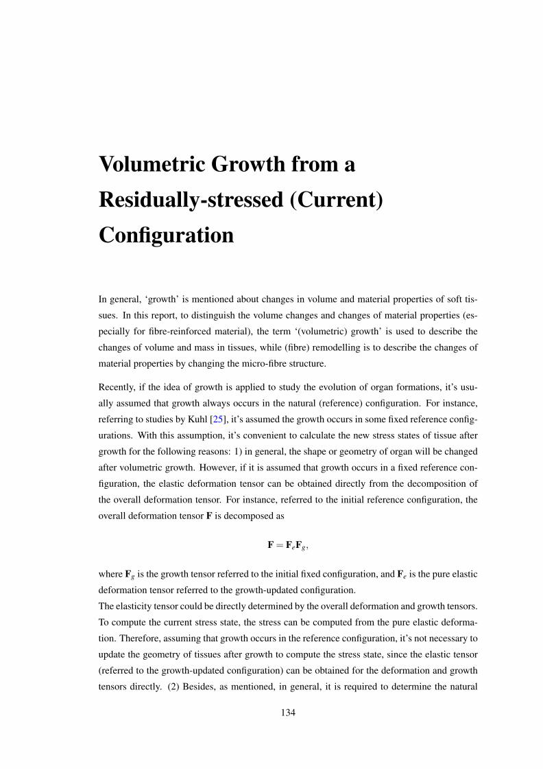
Volumetric Growth from aResidually-stressed (Current)Configuration
In general, ‘growth’ is mentioned about changes in volume and material properties of soft tis-
sues. In this report, to distinguish the volume changes and changes of material properties (es-
pecially for fibre-reinforced material), the term ‘(volumetric) growth’ is used to describe the
changes of volume and mass in tissues, while (fibre) remodelling is to describe the changes of
material properties by changing the micro-fibre structure.
Recently, if the idea of growth is applied to study the evolution of organ formations, it’s usu-
ally assumed that growth always occurs in the natural (reference) configuration. For instance,
referring to studies by Kuhl [25], it’s assumed the growth occurs in some fixed reference config-
urations. With this assumption, it’s convenient to calculate the new stress states of tissue after
growth for the following reasons: 1) in general, the shape or geometry of organ will be changed
after volumetric growth. However, if it is assumed that growth occurs in a fixed reference con-
figuration, the elastic deformation tensor can be obtained directly from the decomposition of
the overall deformation tensor. For instance, referred to the initial reference configuration, the
overall deformation tensor F is decomposed as
F = FeFg,
where Fg is the growth tensor referred to the initial fixed configuration, and Fe is the pure elastic
deformation tensor referred to the growth-updated configuration.
The elasticity tensor could be directly determined by the overall deformation and growth tensors.
To compute the current stress state, the stress can be computed from the pure elastic deforma-
tion. Therefore, assuming that growth occurs in the reference configuration, it’s not necessary to
update the geometry of tissues after growth to compute the stress state, since the elastic tensor
(referred to the growth-updated configuration) can be obtained for the deformation and growth
tensors directly. (2) Besides, as mentioned, in general, it is required to determine the natural
134
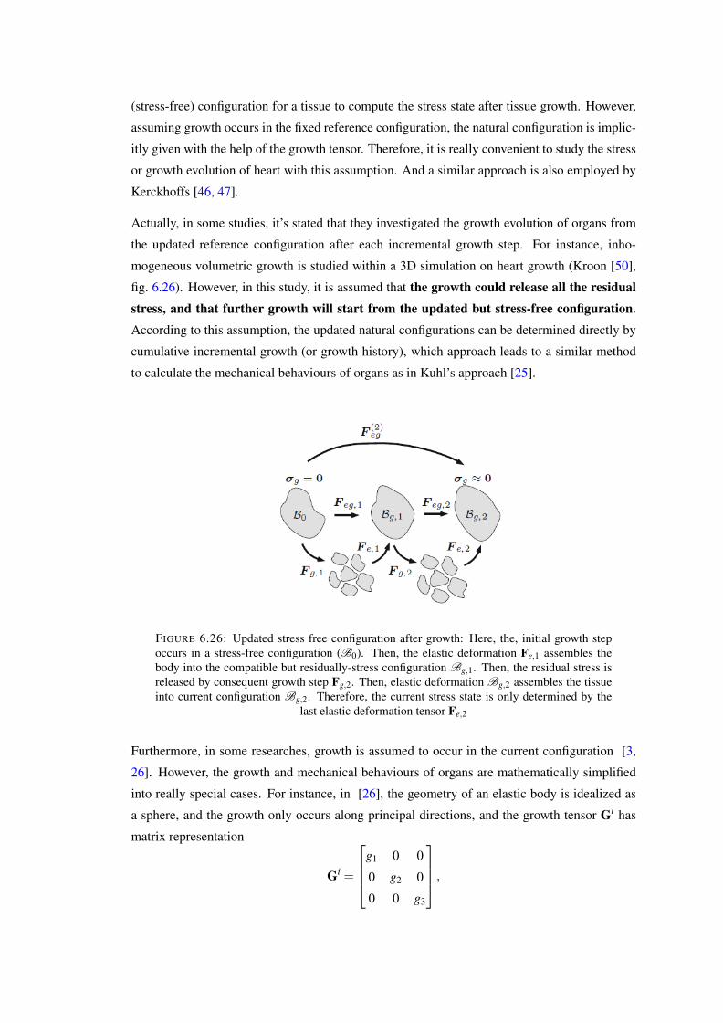
(stress-free) configuration for a tissue to compute the stress state after tissue growth. However,
assuming growth occurs in the fixed reference configuration, the natural configuration is implic-
itly given with the help of the growth tensor. Therefore, it is really convenient to study the stress
or growth evolution of heart with this assumption. And a similar approach is also employed by
Kerckhoffs [46, 47].
Actually, in some studies, it’s stated that they investigated the growth evolution of organs from
the updated reference configuration after each incremental growth step. For instance, inho-
mogeneous volumetric growth is studied within a 3D simulation on heart growth (Kroon [50],
fig. 6.26). However, in this study, it is assumed that the growth could release all the residualstress, and that further growth will start from the updated but stress-free configuration.
According to this assumption, the updated natural configurations can be determined directly by
cumulative incremental growth (or growth history), which approach leads to a similar method
to calculate the mechanical behaviours of organs as in Kuhl’s approach [25].
FIGURE 6.26: Updated stress free configuration after growth: Here, the, initial growth stepoccurs in a stress-free configuration (B0). Then, the elastic deformation Fe,1 assembles thebody into the compatible but residually-stress configuration Bg,1. Then, the residual stress isreleased by consequent growth step Fg,2. Then, elastic deformation Bg,2 assembles the tissueinto current configuration Bg,2. Therefore, the current stress state is only determined by the
last elastic deformation tensor Fe,2
Furthermore, in some researches, growth is assumed to occur in the current configuration [3,
26]. However, the growth and mechanical behaviours of organs are mathematically simplified
into really special cases. For instance, in [26], the geometry of an elastic body is idealized as
a sphere, and the growth only occurs along principal directions, and the growth tensor Gi has
matrix representation
Gi =
g1 0 0
0 g2 0
0 0 g3
,
and with the homogeneous pressure acting on the external surface of the spherical body, the
elastic deformation could be described by the diagonal tensor as
Fie =
λ1 0 0
0 λ2 0
0 0 λ3
.
Then after a sequence of k steps growth, the overall deformation could be stated as
Ak = Gk ·Fke ·Gk−1 ·Fk−1
e · · ·G1 ·F1e ,
and due to diagonal form of growth and deformation tensors, it could be re-arranged as
Ak = Gk ·Gk−1 · · ·G1Fke ·Fk−1
e · · ·F1e .
Similarly with Kuhl’s approach [25], it is computationally convenient to update the reference
configuration by using the cumulative growth tensor in the last equation for the targeted elastic
body and to compute the mechanical behaviours of the body from a new natural configuration.
However, living organs are actually exposed to external loading all the time, while the growth
should occur from the residually-stressed current configuration. In this section, we try to draw
a sketch on 1) how to obtain the constitutive laws of soft tissue after introducing the inhomoge-
neous growth in the residually-stressed current configuration, 2) how to couple the growth and
(fibre) remodelling processes to identify new mechanical behaviours of soft tissue.
6.8 Constitutive laws for Living Organs with Volumetric Growth
In this section, it’s assumed that pure growth doesn’t induce any elastic deformation (H1).
In other words, the mechanical properties do not change after growth.
Besides, it’s also assumed that the incremental growth is determined by external environ-mental cues, which are independent of the subsequent elastic behaviours of tissues. (H2)
6.8.1 Growth from a Natural Configuration
As an easy start, it’s assumed that pure growth, which is pre-determined by a given growth law,
occurs in the natural (stress-free) configuration. Then the local growth tensor deforms the elastic
body into an incompatible and stress-free configuration B2. After applying loading, the living
organ eventually deforms into a stressed and compatible configuration B3 (fig. 6.27).
FIGURE 6.27: Growth from the stress-free configuration: It’s assumed incremental growth step(Fg) deforms the tissues from the (incompatible) natural configuration B1 into the updated (andincompatible) configuration B2. Then, the elastic deformation Fe assembles the tissues into the
compatible configuration B3.
With help of H1, the overall elastic energy from B1 to B3 could be expressed as
W1 = JgW2, (6.62)
where W1 is the elastic strain energy from B1 to B3 (W1 =W1(A)), W2 is the elastic strain energy
from B2 to B3 (W2 =W1(Fe)), and Jg is the determinant of the growth tensor Fg.
To calculate the Cauchy stress From B2, actually, only pure elastic behaviour is involved (no
growth) and the Cauchy stress is expressed as
σ = J−1e Fe
∂W2
∂Fe. (6.63)
From B1, with help of eq. (6.62), the Cauchy stress could be expressed as
σ = J−1A A
∂W1
∂A= J−1
A A∂ (JgW2)
∂A= J−1
A JgA(∂Fe
∂A:
∂W2
∂Fe) = J−1
e Fe∂W2
∂Fe, (6.64)
where A = FeFg.
It’s worth to emphasize that the growth tensor is determined by certain growth laws (related to
external environmental cues), which indicates that the pure growth tensor is independent of the
elastic deformation tensor,∂Fg
∂Fe= 0.
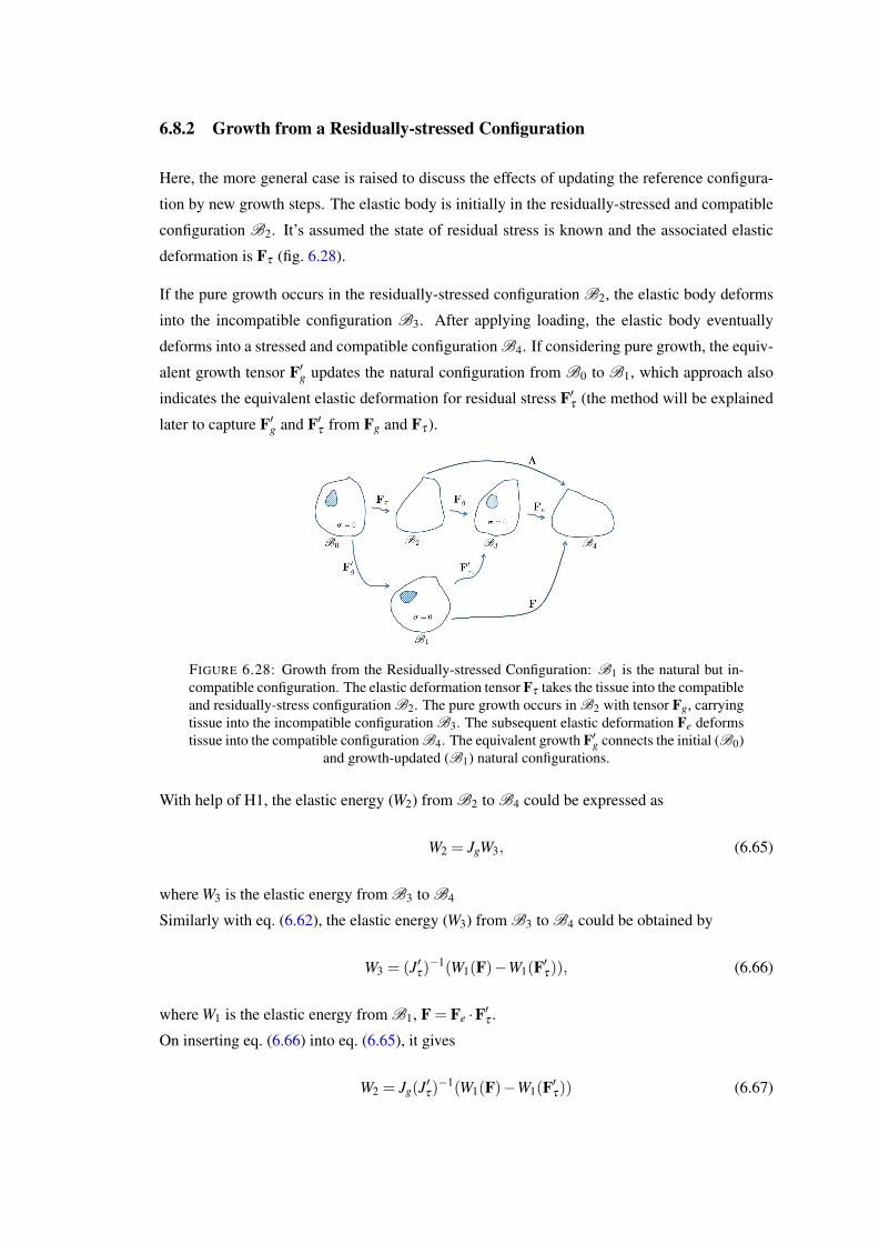
6.8.2 Growth from a Residually-stressed Configuration
Here, the more general case is raised to discuss the effects of updating the reference configura-
tion by new growth steps. The elastic body is initially in the residually-stressed and compatible
configuration B2. It’s assumed the state of residual stress is known and the associated elastic
deformation is Fτ (fig. 6.28).
If the pure growth occurs in the residually-stressed configuration B2, the elastic body deforms
into the incompatible configuration B3. After applying loading, the elastic body eventually
deforms into a stressed and compatible configuration B4. If considering pure growth, the equiv-
alent growth tensor F′g updates the natural configuration from B0 to B1, which approach also
indicates the equivalent elastic deformation for residual stress F′τ (the method will be explained
later to capture F′g and F′τ from Fg and Fτ ).
FIGURE 6.28: Growth from the Residually-stressed Configuration: B1 is the natural but in-compatible configuration. The elastic deformation tensor Fτ takes the tissue into the compatibleand residually-stress configuration B2. The pure growth occurs in B2 with tensor Fg, carryingtissue into the incompatible configuration B3. The subsequent elastic deformation Fe deformstissue into the compatible configuration B4. The equivalent growth F′g connects the initial (B0)
and growth-updated (B1) natural configurations.
With help of H1, the elastic energy (W2) from B2 to B4 could be expressed as
W2 = JgW3, (6.65)
where W3 is the elastic energy from B3 to B4
Similarly with eq. (6.62), the elastic energy (W3) from B3 to B4 could be obtained by
W3 = (J′τ)−1(W1(F)−W1(F′τ)), (6.66)
where W1 is the elastic energy from B1, F = Fe ·F′τ .
On inserting eq. (6.66) into eq. (6.65), it gives
W2 = Jg(J′τ)−1(W1(F)−W1(F′τ)) (6.67)
Two methods are employed here to compute the Cauchy stress in B4:
(1) From B1,
σ = J−1F F
∂W1
∂F(6.68)
(2) From B2, with help of eq. (6.67), the Cauchy stress is given as
σ = J−1A A
∂W2
∂A= J−1
A A∂[JgJ′−1
τ (W1(F)−W1(F′τ))]
∂A
= J−1A A
∂[JgJ′−1
τ (W1(F))]
∂A− J−1
A A∂[JgJ′−1
τ (W1(F′τ))]
∂A
= J−1F A( ∂F
∂A) : (
∂W1(F)∂F
)= J−1F F
∂W1
∂F
(6.69)
where A = FeFg, F = FeF′τ .
The simplified Cauchy stresses give the same expressions as in eq. (6.68) and (6.69), which
indicates that the new SEF (eq. (6.67)) is appropriate.
Then, the only undefined terms are the equivalent growth F′g and elastic deformation F′τ . To
determine F′g, the polar decomposition of Fτ is needed:
Fτ = VτRτ . (6.70)
Here, it is considered that an arbitrary material point of elastic body is rotated with tensor Rτ ,
then, the rotated configuration BR is deformed into B1 by tensor Vτ . For pure growth, the
growth tensor could be decomposed as
Fg = RgUg. (6.71)
Growth tensor Fg is with respect to B1. However, if considering the effect of growth in changing
the shape of initial body, it could give an equivalent growth occurs before elastic deformation,
by rotating the growth tensor back into the initial configuration B0 with the tensor Rτ the de-
composition of Fg could help to raise the form of F′g, with help of eq. (6.71), as
Fg = RgUg ⇒ F′g = R−1τ RgUg(R−1
τ )T . (6.72)
And with rotations between orthogonal coordinates (RTτ Rτ = I), eq. (6.72) could be re-written
as
F′g = RTτ RgUgRτ . (6.73)
The deformation path (B0→B1→B3) is equivalent to path (B0→B2→B3), so that
FgFτ = F′τF′g (6.74)
and hence
F′τ = FgFτ(F′g)−1 (6.75)
Example (2D growth) A living body is deformed with the elastic deformation tensor Fe from
initial configuration B0 (fig. 6.29). Considering here, the material point is firstly rotated by Re
and then stretched by Ve as
Fe = VeRe.
If the initial basis vectors (e1,e2) of coordinates are rotated to new ones (e′1,e′2) with rotation
angle π
3 , then the matrix form of the rotation tensor is given as
Re =
[cos π
3 sin π
3
−sin π
3 cos π
3
].
where component Rei j = e′i · e j.
Assuming the body is stretched into B3 with Ve as
Ve = I+(λe−1)e′1⊗ e′1.
then, the body grows along the e′2 direction in BV as
Fg = I+(λg−1)e′2⊗ e′2.
Fgi = λg f f⊗ f+λgss⊗ s+λgnn⊗ n
What’s the equivalent growth for this living body?
Solution Obviously, if skipping the elastic deformation, equivalently saying, the living body
grows along the e2 direction with growth tensor from B0 as
F′g = I+(λg−1)e2⊗ e2 =
[1 0
0 λg
].
giving the updated stress-free configuration B1.
Recalling eq. (6.73), the equivalent growth tensor is given as
F′g = RTe FgRe = I+(λg−1)e2⊗ e2
Comparing last two equations describing the equivalent growths, it shows a good validation for
algorithm from eq. (6.71) to (6.73).
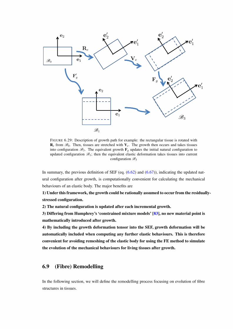
FIGURE 6.29: Description of growth path for example: the rectangular tissue is rotated withRe from B0. Then, tissues are stretched with Ve. The growth then occurs and takes tissuesinto configuration B3. The equivalent growth Fg updates the initial natural configuration toupdated configuration B1; then the equivalent elastic deformation takes tissues into current
configuration B3
In summary, the previous definition of SEF (eq. (6.62) and (6.67)), indicating the updated nat-
ural configuration after growth, is computationally convenient for calculating the mechanical
behaviours of an elastic body. The major benefits are
1) Under this framework, the growth could be rationally assumed to occur from the residually-stressed configuration.2) The natural configuration is updated after each incremental growth.3) Differing from Humphrey’s ‘constrained mixture models’ [83], no new material point ismathematically introduced after growth.4) By including the growth deformation tensor into the SEF, growth deformation will beautomatically included when computing any further elastic behaviours. This is thereforeconvenient for avoiding remeshing of the elastic body for using the FE method to simulatethe evolution of the mechanical behaviours for living tissues after growth.
6.9 (Fibre) Remodelling
In the following section, we will define the remodelling process focusing on evolution of fibre
structures in tissues.
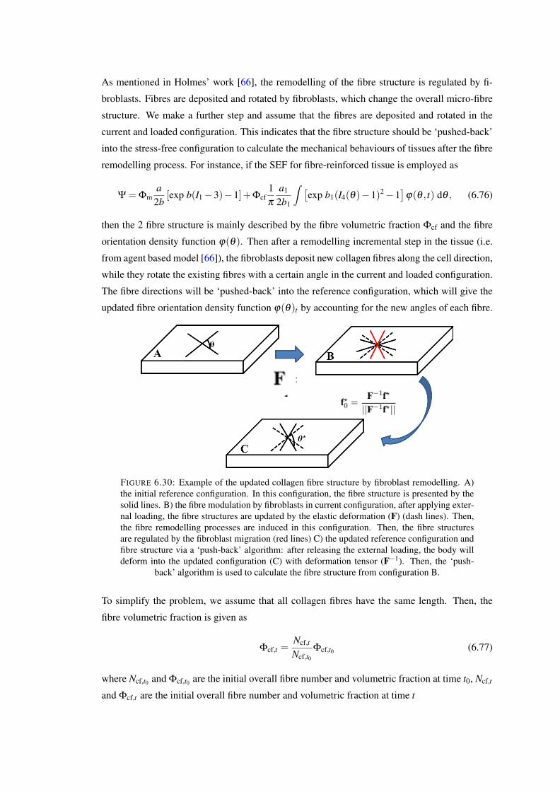
As mentioned in Holmes’ work [66], the remodelling of the fibre structure is regulated by fi-
broblasts. Fibres are deposited and rotated by fibroblasts, which change the overall micro-fibre
structure. We make a further step and assume that the fibres are deposited and rotated in the
current and loaded configuration. This indicates that the fibre structure should be ‘pushed-back’
into the stress-free configuration to calculate the mechanical behaviours of tissues after the fibre
remodelling process. For instance, if the SEF for fibre-reinforced tissue is employed as
Ψ = Φma2b
[exp b(I1−3)−1]+Φcf1π
a1
2b1
∫ [exp b1(I4(θ)−1)2−1
]ϕ(θ , t) dθ , (6.76)
then the 2 fibre structure is mainly described by the fibre volumetric fraction Φcf and the fibre
orientation density function ϕ(θ). Then after a remodelling incremental step in the tissue (i.e.
from agent based model [66]), the fibroblasts deposit new collagen fibres along the cell direction,
while they rotate the existing fibres with a certain angle in the current and loaded configuration.
The fibre directions will be ‘pushed-back’ into the reference configuration, which will give the
updated fibre orientation density function ϕ(θ)t by accounting for the new angles of each fibre.
FIGURE 6.30: Example of the updated collagen fibre structure by fibroblast remodelling. A)the initial reference configuration. In this configuration, the fibre structure is presented by thesolid lines. B) the fibre modulation by fibroblasts in current configuration, after applying exter-nal loading, the fibre structures are updated by the elastic deformation (F) (dash lines). Then,the fibre remodelling processes are induced in this configuration. Then, the fibre structuresare regulated by the fibroblast migration (red lines) C) the updated reference configuration andfibre structure via a ‘push-back’ algorithm: after releasing the external loading, the body willdeform into the updated configuration (C) with deformation tensor (F−1). Then, the ‘push-
back’ algorithm is used to calculate the fibre structure from configuration B.
To simplify the problem, we assume that all collagen fibres have the same length. Then, the
fibre volumetric fraction is given as
Φcf,t =Ncf,t
Ncf,t0Φcf,t0 (6.77)
where Ncf,t0 and Φcf,t0 are the initial overall fibre number and volumetric fraction at time t0, Ncf,t
and Φcf,t are the initial overall fibre number and volumetric fraction at time t
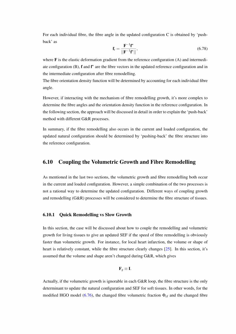
For each individual fibre, the fibre angle in the updated configuration C is obtained by ‘push-
back’ as
ft =F−1f?
||F−1f?|| , (6.78)
where F is the elastic deformation gradient from the reference configuration (A) and intermedi-
ate configuration (B), f and f? are the fibre vectors in the updated reference configuration and in
the intermediate configuration after fibre remodelling.
The fibre orientation density function will be determined by accounting for each individual fibre
angle.
However, if interacting with the mechanism of fibre remodelling growth, it’s more complex to
determine the fibre angles and the orientation density function in the reference configuration. In
the following section, the approach will be discussed in detail in order to explain the ‘push-back’
method with different G&R processes.
In summary, if the fibre remodelling also occurs in the current and loaded configuration, the
updated natural configuration should be determined by ‘pushing-back’ the fibre structure into
the reference configuration.
6.10 Coupling the Volumetric Growth and Fibre Remodelling
As mentioned in the last two sections, the volumetric growth and fibre remodelling both occur
in the current and loaded configuration. However, a simple combination of the two processes is
not a rational way to determine the updated configuration. Different ways of coupling growth
and remodelling (G&R) processes will be considered to determine the fibre structure of tissues.
6.10.1 Quick Remodelling vs Slow Growth
In this section, the case will be discussed about how to couple the remodelling and volumetric
growth for living tissues to give an updated SEF if the speed of fibre remodelling is obviously
faster than volumetric growth. For instance, for local heart infarction, the volume or shape of
heart is relatively constant, while the fibre structure clearly changes [25]. In this section, it’s
assumed that the volume and shape aren’t changed during G&R, which gives
Fg ≡ I.
Actually, if the volumetric growth is ignorable in each G&R loop, the fibre structure is the only
determinant to update the natural configuration and SEF for soft tissues. In other words, for the
modified HGO model (6.76), the changed fibre volumetric fraction Φcf and the changed fibre
orientation density function ϕ(θ , t) are the parameters to describe the new SEF related with the
updated natural configuration after G&R process. For details of this process, we refer to the last
section.
6.10.2 Quick Growth vs Slow Remodelling
In this section, the case will be discussed about coupling the remodelling and volumetric growth
for living tissues to give an updated SEF if the speed of volumetric growth is obviously faster
than fibre remodelling. Here, we assume the fibre structure is not actively modulated by fibrob-
lasts but responds passively to the volumetric growth of the matrix tissue.
FIGURE 6.31: Quick growth vs slow remodelling: the fibre orientation is modified by thegrowth. B0 is the natural (but incompatible) configuration, Fτ is the elastic deformation con-necting the natural (B0) and residually-stress configurations (B2) . Incremental growth stepFg carries body into B3. The updated natural configuration B1 is obtained by the equivalentelastic deformation tensor F′τ between B1 and B3. Then, the new fibre angle in B1 can be
obtained by ‘push-forwards’ old fibre angle from B0 with equivalent growth tensor F′g.
The growth of the matrix material is induced for the elastic body from the loaded configuration.
If the total number of fibres is constant during growth, the fibre volumetric fraction is updated
as
Φcf =Φcf,t0
Jg, (6.79)
where Jg is the determinant of the growth tensor Fg, Φcf,t0 is the initial fibre volumetric fraction.
And due to the growing deformation, the fibre angles in the initial natural configuration B0
should be ‘pushed-forward’ into the updated natural configuration B1 (fig. 6.31) as
f1 =F′gf0
||F′gf0||, (6.80)
where f1, f0 are the fibre vectors in B1 and B0.
Moreover, as mentioned in Section 1.2, the SEF is calculated after the volumetric growth from
the residually-stressed configuration. By coupling with the fibre remodelling, the volumetric
fraction and the fibre orientation density function are updated (by eq. (6.79), (6.80) and (6.15))
as well.
6.10.3 Quick Growth vs Quick Remodelling
In this section, the growth and remodelling are assumed to take place with similar speeds, i.e.
the growth and remodelling processes occur simultaneously from the loaded configuration. This
idea is quite similar to the assumption of the mixture of ‘constant individual density (CID)’
and ‘adaptive individual density (AID)’ by Watton et al. [16]. Besides, here, we also assume
the incremental growth step occurs after the incremental fibre remodelling step. And we try to
include this G&R process under the coupled G&R framework to describe the evolution of the
mechanical behaviours of living tissues.
It’s assumed that the volumetric growth and fibre remodelling occur in the loaded configura-
tion B2 (regulated by different but given G&R laws fig. 6.31). If the overall fibre number is
increased to Ncf,t from the initial value Ncf,t0 by active fibre remodelling (as for the agent-based
model [66]), the updated fibre remodelling fraction is
Φcf,t =Φcf,t0
Jg
Ncf,t
Ncf,t0, (6.81)
where Ncf,t is the updated fibre number at time t.
For the individual fibre, the unit fibre vector (f2) is updated by the fibre remodelling process,
(i.e. modified by the fibroblast migration), in intermediate configurations B2 in fig. 6.28, while
the updated fibre vector is given as f?2.
Then, the fibre should be ‘pushed-back’ into the updated reference configuration (B1 in fig. 6.28),
which gives
f1 =(F′τ)−1Fgf?2||(F′τ)−1Fgf?2||
, (6.82)
where F′τ is the elastic deformation tensor defined in eq. (6.67).
To determine the updated SEF after both fibre remodelling and volumetric growth, the general
form of the SEF could be expressed as eq. (6.67) (indicating a volumetric growth from the
loaded configuration), but the updated fibre volumetric fraction in eq. (6.81) and fibre orientation
density function should be inserted into the SEF to describe the fibre remodelling in the current
configuration.
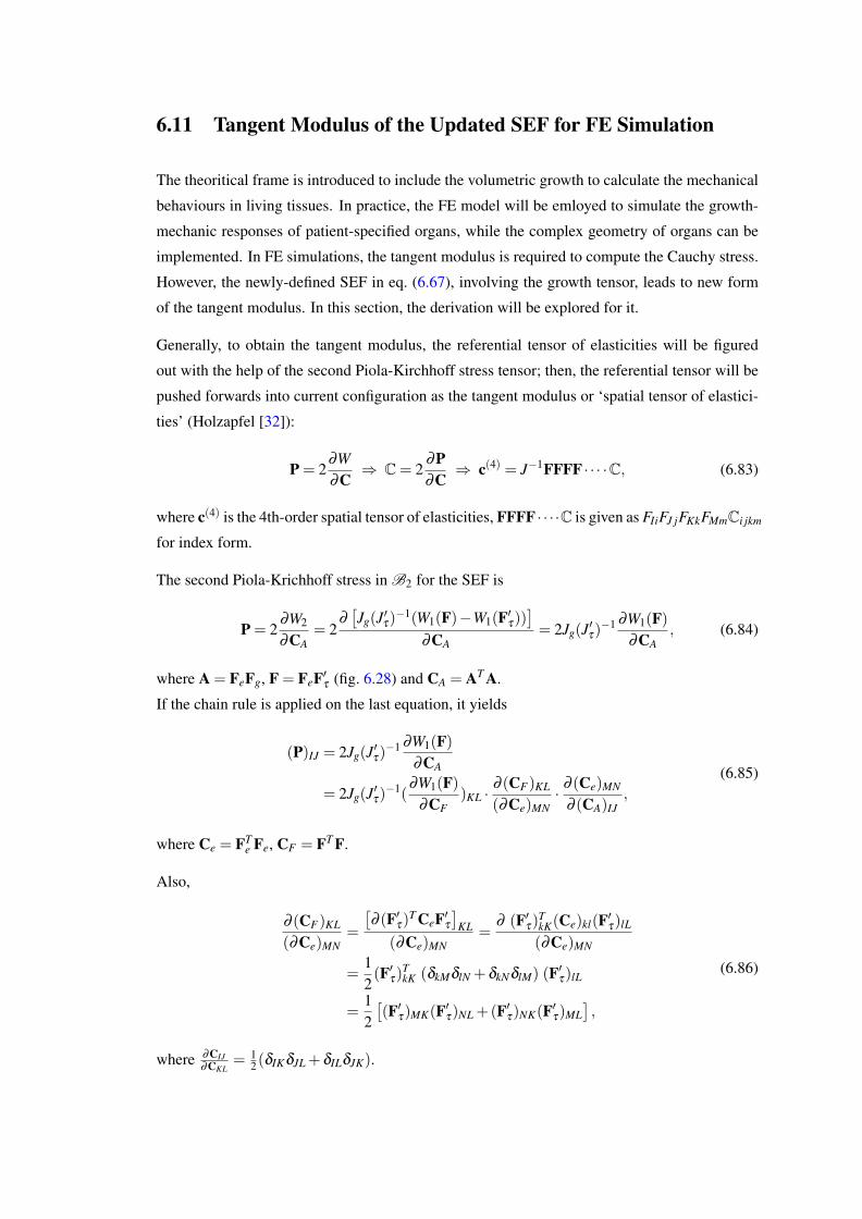
6.11 Tangent Modulus of the Updated SEF for FE Simulation
The theoritical frame is introduced to include the volumetric growth to calculate the mechanical
behaviours in living tissues. In practice, the FE model will be emloyed to simulate the growth-
mechanic responses of patient-specified organs, while the complex geometry of organs can be
implemented. In FE simulations, the tangent modulus is required to compute the Cauchy stress.
However, the newly-defined SEF in eq. (6.67), involving the growth tensor, leads to new form
of the tangent modulus. In this section, the derivation will be explored for it.
Generally, to obtain the tangent modulus, the referential tensor of elasticities will be figured
out with the help of the second Piola-Kirchhoff stress tensor; then, the referential tensor will be
pushed forwards into current configuration as the tangent modulus or ‘spatial tensor of elastici-
ties’ (Holzapfel [32]):
P = 2∂W∂C
⇒ C= 2∂P∂C⇒ c(4) = J−1FFFF · · · ·C, (6.83)
where c(4) is the 4th-order spatial tensor of elasticities, FFFF · · ··C is given as FIiFJ jFKkFMmCi jkm
for index form.
The second Piola-Krichhoff stress in B2 for the SEF is
P = 2∂W2
∂CA= 2
∂[Jg(J′τ)
−1(W1(F)−W1(F′τ))]
∂CA= 2Jg(J′τ)
−1 ∂W1(F)∂CA
, (6.84)
where A = FeFg, F = FeF′τ (fig. 6.28) and CA = AT A.
If the chain rule is applied on the last equation, it yields
(P)IJ = 2Jg(J′τ)−1 ∂W1(F)
∂CA
= 2Jg(J′τ)−1(
∂W1(F)∂CF
)KL ·∂ (CF)KL
(∂Ce)MN· ∂ (Ce)MN
∂ (CA)IJ,
(6.85)
where Ce = FTe Fe, CF = FT F.
Also,
∂ (CF)KL
(∂Ce)MN=
[∂ (F′τ)T CeF′τ
]KL
(∂Ce)MN=
∂ (F′τ)TkK(Ce)kl(F′τ)lL
(∂Ce)MN
=12(F′τ)
TkK (δkMδlN +δkNδlM) (F′τ)lL
=12[(F′τ)MK(F′τ)NL +(F′τ)NK(F′τ)ML
],
(6.86)
where ∂CIJ∂CKL
= 12(δIKδJL +δILδJK).
Similarly,
∂ (Ce)MN
(∂CA)IJ=
12[(F−1
g )IM(F−1g )JN +(F−1
g )JM(F−1g )IN
], (6.87)
where Ce = (F−1g )T CAF−1
g .
Inserting eq. (6.86) and (6.87) into eq. (6.85) gives
P = Jg(J′τ)−1A(6)(
∂W1
∂CF)KL, (6.88)
where A(6) = 12 [(F
′τ)MK(F′τ)NL +(F′τ)NK(F′τ)ML]
[(F−1
g )IM(F−1g )JN +(F−1
g )JM(F−1g )IN
].
Then, referential tensor of elasticities is
C= 2∂ (P)IJ
(∂CA)PQ= 2
∂ (P)IJ
(∂CF)RT· ∂ (CF)RT
(∂CA)PQ
= 2Jg(J′τ)−1A(6)
( ∂W1∂CF
)KL
∂ (CF)RT· ∂ (CF)RT
(∂Ce)XY· ∂ (Ce)XY
(∂CA)PQ
= Jg(J′τ)−1A(6) ∂W1
∂ (CF)KL∂ (CF)RTB(6),
(6.89)
where B(6) = 12 [(F
′τ)XR(F′τ)Y T +(F′τ)Y R(F′τ)XT ]
[(F−1
g )PX(F−1g )QY +(F−1
g )QX(F−1g )PY
].
Then, the tangent modulus or spatial tensor o f elasticities is obtained as
c(4) = J−1A AAAA · · · ·C
= J−1A Jg(J′τ)
−1AiIA jJApPAqQA(6) ∂W1
∂ (CF)KL∂ (CF)RTB(6)
= J−1F (Fe)iU(Fg)UI(Fe) jV (Fg)V J(Fe)pA(Fg)AP(Fe)qB(Fg)BQA(6) ∂W1
∂ (CF)KL∂ (CF)RTB(6).
(6.90)
By arranging last equation, it gives
c(4) = J−1F (Fe)iU(Fe) jV (Fe)pA(Fe)qB(Fg)UI(Fg)V J(Fg)AP(Fg)BQG(8)R(8) ∂W1
∂ (CF)KL∂ (CF)RT,
(6.91)
where G(8)= 12
[(F−1
g )IM(F−1g )JN +(F−1
g )JM(F−1g )IN
][(F−1
g )PX(F−1g )QY +(F−1
g )QX(F−1g )PY
], and
R(8) = 12 [(F
′τ)MK(F′τ)NL +(F′τ)NK(F′τ)ML] [(F′τ)XR(F′τ)Y T +(F′τ)Y R(F′τ)XT ] .
To the simply last equation, it gives
(Fg)UI(Fg)V J(Fg)AP(Fg)BQG(8) =12(δUMδV N +δV MδUL)(δAX δBY +δAY δBX). (6.92)
Then, use of eq. (6.92) and R(8) gives
(Fg)UI(Fg)V J(Fg)AP(Fg)BQG(8)R(8) =[(F′τ)UK(F′τ)V L +(F′τ)V K(F′τ)UL
]
∗[(F′τ)AR(F′τ)BT +(F′τ)AT (F′τ)BR
].
(6.93)
Inserting eq. (6.93) into eq. (6.91) yields
c(4) =J−1F (Fe)iU(Fe) jV (Fe)pA(Fe)qB[(F′τ)UK(F′τ)V L +(F′τ)V K(F′τ)UL
]
[(F′τ)AR(F′τ)BT +(F′τ)AT (F′τ)BR
] ∂W1
∂ (CF)KL∂ (CF)RT.
(6.94)
Since F = FeF′τ , eq. (6.94) gives
c(4) = J−1F [(F)iK(F) jL +(F)iL(F) jK ]
[(F)pR(F)qT +(F)pT (F)qR]∂W1
∂ (CF)KL∂ (CF)RT.
(6.95)
And due to the symmetry in the 4th order tensor ∂W1∂ (CF )KL∂ (CF )RT
, eq. (6.95) yields
c(4) = J−1F 4FiKF jLFpRFqT
∂W1
∂ (CF)KL∂ (CF)RT. (6.96)
Actually, referring to B1 in fig. 6.28, spatial tensor o f elasticities in B4 could be also derived
as
c(4) = J−1F 4FiKF jLFpRFqT
∂W1
∂ (CF)KL∂ (CF)RT. (6.97)
6.12 Summary
In previous researches, to calculate the mechanical behaviours of living organs, it’s usually
assumed that growth occurs in the natural (reference) configuration. Or it is assumed that the
growth could release all the residual stress, and that further growth will start from the updated
but stress-free configuration.
In this work, a theoretical framework is developed to calculate the mechanical behaviours of soft
tissue after introducing inhomogeneous growth in a residually-stressed current configuration.
Under this framework, the growth could be rationally assumed to occur from the residually-
stressed configuration, which avoids to assume the growth occurs in a ‘virtual’ reference con-
figuration in many previous researches. Moreover, growth deformation will be automatically
included when computing any further elastic behaviours by the SEF related to growth-updated

configurations. The theoretical framework is introduced to couple the growth and fibre remod-
elling process to describe the mechanical behaviours of living tissues.
Conclusion and Future Work
6.13 Limitations
The discussions for the calculation results haven been presented in previous chapters. Some
limitations will be discussed here.
6.13.1 Multiple Cut Model to Estimate the Residual Stress in LV
In Chapter 5, to develop the heart tube model, all the geometrical information is obtained from
the experiments from Omens’ work [59], including the geometry of heart tube and opening
angles for heart slices after cuts. However, the experimental data are limited, for instance, the
geometry of the heart in our model is measured from one photograph of a typical short-axis
apical slice of a mouse heart [59]. More experiments are needed to improve the measurement
for the geometry of hearts.
Considering the geometric changes after cutting, it is assumed that the heart tube will deform
into the new circular cylindrical configuration after multiple cuts. However, due to the impact
of shear stress, the heart might not maintain a cylindrical configuration after cutting, which will
change the expression of the deformation tensor (like eq. (5.10)) in our work. Besides, the
residual stress is induced by the complex growth processes during the life of heart. Previous
work shows that the 3d residual stress distribution should be considered [36] to estimate the
mechanical behaviour of living tissues, which leads to 3d residual strain. In our work, only
circumferential and radial residual strains (2d distribution of residual strain) are considered,
which are measurable by radial opening cuts.
A single fibre family is employed to describe the fibre structure of heart. The dispersed fibre
families are experimentally observed, which are also used in our later works. The mechanical
behaviour of heart tissues will be different with dispersed fibre families, whose effect is not
included in this work.
150
Some revious research suggests that infinite cuts are needed to release all the residual stress in
living tissues. In our model, we developed a 4-cut model rather than a model with more cuts, due
to lack of sufficient experimental data. Further experimental evidence is needed to demonstrate
whether 4-cut is sufficient to release most of the residual stress in the heart.
6.13.2 Coupled Agent-based and FE Model for MI after Infarction
In our work, an idealized half ellipsoid geometry is used to construct FE model for a rat LV.
However, in reality, the geometry of LV is much more complex. With the real (and complex)
geometry of LV, the mechanical behaviours might be different, which might lead to different
mechanical cues and then induce the different migration processes of fibroblast.
The chemokine concentration is assumed to static during the healing process of MI as
∂C∂ t
= 0.
In practice, the chemokine concentration responds to the bio-environment of the LV and changes
with time; for instance, the nutrition concentration is changed with the healing process. With the
time-varied chemokine concentration, the chemokine cue is different from the one in our model,
which gives the different patterns of fibroblast migration. It affects the remodelling process of
MI in LV.
In our model, the fibroblast is assumed to be a rigid sphere, passively responding to external
cues. However, the real fibroblast is deformable, which also contributes to the mechanical be-
haviours of heart tissues. In our future work, the deformation of fibroblasts will be included, as
well as its mechanical contribution for heart functions.
In general, during the heart healing, the remodelling and growth coincidently occur to regu-
late the heart function. In our coupled model, the (volumetric) growth is ignored, while only
the fibre remodelling is investigated. However, the overall mechanical behaviour is affected by
the (volumetric) growth of tissues. For instance, the fibre structure is modified by (volumetric)
growth (discussed in Chapter 7), which will change the material properties of infarcted tissues.
As a result, the mechanical cues will be influenced by growth, which changes the fibre remod-
elling. For a global view, the interaction between remodelling and growth should be considered
to predict the heart function during healing process.
6.14 Conclusion
This thesis focuses on the interactions between mechanical behaviour and G&R processes for
living organs. According to nonlinear elastic theories, residual stress, induced by complex G&R
processes, is of importance to affect the subsequent mechanical responses of soft tissues to
external loading. Here, a multiple cut model is developed to estimate residual stress induced by
G&R processes in the heart, which helps to explain recent experiments on residual stress.
To simulate the G&R process during MI, a multiscale algorithm is employed to couple (organ-
level) three-dimensional heart models with (cell level) agent-based models. Our models capture
interactions and information exchange processes between mechanical behaviour and collagen
tissue remodelling guided by bio-environmental cues.
In addition, a volumetric growth approach is developed to simulate the inhomogeneous growth
in the residually-stressed current configuration for a living organ, which will be embedded into
simulations of the heart G&R process.
In Chaper 5, multiple-cut models are developed to estimate the residual stress distributions in
the LVs of mice, inspired by experimental observation by [59]. They show that both radial and
circumferential cuts are required to release the residual stresses. Remarkably, the results suggest
that using radial cuts alone leads to significantly underestimated residual stress. As mentioned
in previous researches, it suggests many cuts are needed to release all residual stress in living
organs, since residual stress is induced by the complex (inhomogeneous) growth. Accordingly,
our 4-cut model may give better estimations for residual stress than the 2-cut model. This con-
clusion is also supported by the estimated residual stress distributions. As shown in Chapter 5,
stress distributions are smoother when estimated by the 4-cut model, but with a similar magni-
tude to the 2-cut model. The stress states estimated by the 4-cut model are more reasonable for
living organs.
The computational results also explain experimental observation by Fung [3] who concluded that
a single cut can release all residual stress in the residually stressed configuration of an artery,
since the subsequent radial cuts don’t introduce any more elastic deformations. Our models sup-
port that the 1-cut configuration is not the stress free configuration for living organs. More cuts
are needed to release the residual stress and address the stress-free configuration for the heart
during MI healing.
In Chapter 6, a multiscale model is developed by coupling an agent-based model with a three-
dimensional left ventricle model. To simulate the appropriate material properties for myocardium,
a proper fibre tension-compression ‘switch’ is developed in constitutive laws of LV tissues. The
time-dependent model captures the interaction and information exchange process between me-
chanical behaviour and collagen tissue remodelling guided by various external cues. The sim-
ulations show shapes and the locations of infarctions could affect the mechanical behaviour of
total LV and the local collagen cumulation.
For fibre structure, the mean angle of fibre structure decreases near the endosurface for a cir-
cular infarction while it decreases less for the elliptical infarction. At the infarction centre,
the anisotropy of the fibre structure for a circular infarction, reflected by kurtosis of the fibre
structure, increases more.
For stress states, in the FE model, the overall stress distributions are significantly changed dur-
ing MI processes for the heart with circular or elliptical infarctions. The stress concentrations
are obviously in the infarcted regions. For strain, the evolution of strain fits with the experimen-
tal observations for both infarctions. However, strains decrease more for tissues with elliptical
infarctions.
A theoretical framework is developed to calculate the mechanical behaviours of soft tissue af-
ter introducing inhomogeneous growth in a residually-stressed current configuration. Under this
framework, the growth could be rationally assumed to occur from the residually-stressed config-
uration, which avoids to assume the growth occurs in a ‘virtual’ reference configuration in many
previous researches. Moreover, growth deformation will be automatically included when com-
puting any further elastic behaviours by the SEF related to growth-updated configurations. For
this sake, it gives the convenience to avoid remeshing the elastic body under FE computational
framework.
6.15 Future Work
For the multiple-cut model in Chapter 4, the tissues are assumed to be composed with matrix
material and a single fibre family. However, according to experiments by [70], the fibre ori-
entation is dispersed, while the fibre structure could be considered as dispersed fibre families.
Therefore, the constitutive laws for tissues could be modified with a fibre orientation density
function for the tissues with dispersed fibre families. For instance, the constitutive law (HO
model) in Chapter 3 is employed as
Ψ = Ψm +Ψf, (6.98)
where
Ψm =a2bexp[b(I1−3)]−1, Ψf =
af
2bfexp[bf(I4−1)2]−1, (6.99)
a,b,af,bf are material constants, and
I1 = tr(C), I4 = f0 · (Cf0), (6.100)
I1 and I4 being the invariants corresponding to the matrix and fibre structure of the myocardium.
And considering the 2d dispersed fibre families, the SEF for fibre Ψf is rewritten as
Ψf =1π
af
2bf
∫ [exp bf(I4(Θ)−1)2−1
]ϕ(Θ) dΘ, (6.101)
where af,bf are the material parameters for fibres, ϕ(θ) is the fibre orientation density function
and Θ is the angle to a specified orientation.
This SEF can give a better estimation for the stress-strain relation for heart tissues. Besides, as
mentioned in Chapter 5, the shear stress will be introduced if the SEF is only including a single
fibre family. With dispersed (and symmetric) fibre families, the distribution of shear stresses
will be symmetry as the fibre structure, while the effects by shear stress will be further reduced
due to symmetry of fibre structure (the example can be found at section 5.4.1).
In Chapter 5, according to experimental observations by Omens, we assumed 2 or 4 cuts can
release the residual stress in LV tube. However, if experimental data are available for opening
angle measurements with even more cuts, the residual stress can be estimated by multiple-cut
models, which can improve the residual stress estimation. Besides, it can prove the validation
on questions whether the 4-cut model gives reasonable estimations for the residual stress, even
though the 4-cut model has advantages compared with previous single cut models.
The approaches for fibre remodel (Chapter 6) and volumetric growth (Chapter 7) are both pre-
sented in our researches. Furthermore, our academic ambition is to develop a framework to
investigate the heart remodelling and growth of the heart by coupling the remodelling of fibre
structure and volumetric growth through a multiscale model.
As mentioned in Chapters 6 and 7, the volumetric growth and fibre remodelling both occur in
the current and loaded configurations. However, the simple combination of the two processes
is not a rational way to determine the updated reference configuration and mechanical response
of tissues. The different ways of coupling G&R processes will be considered to determine the
mechanical behaviour of the fibre-reinforced tissues during G&R processes.
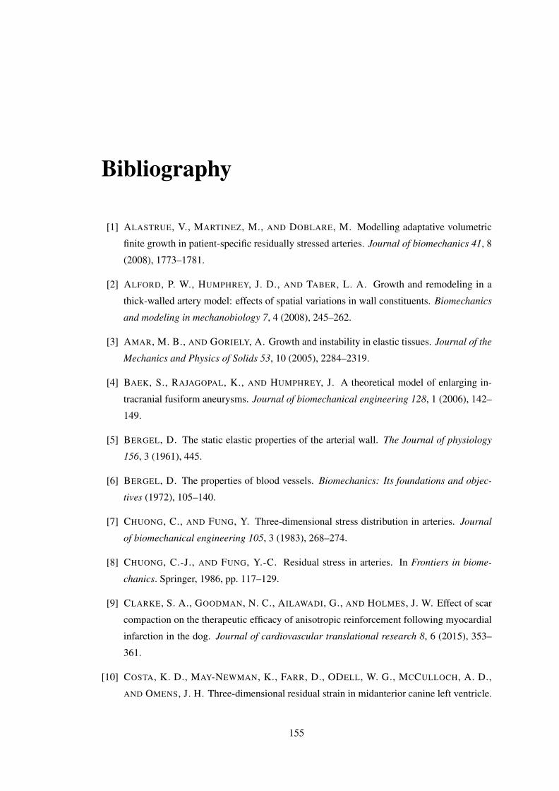
Bibliography
[1] ALASTRUE, V., MARTINEZ, M., AND DOBLARE, M. Modelling adaptative volumetric
finite growth in patient-specific residually stressed arteries. Journal of biomechanics 41, 8
(2008), 1773–1781.
[2] ALFORD, P. W., HUMPHREY, J. D., AND TABER, L. A. Growth and remodeling in a
thick-walled artery model: effects of spatial variations in wall constituents. Biomechanics
and modeling in mechanobiology 7, 4 (2008), 245–262.
[3] AMAR, M. B., AND GORIELY, A. Growth and instability in elastic tissues. Journal of the
Mechanics and Physics of Solids 53, 10 (2005), 2284–2319.
[4] BAEK, S., RAJAGOPAL, K., AND HUMPHREY, J. A theoretical model of enlarging in-
tracranial fusiform aneurysms. Journal of biomechanical engineering 128, 1 (2006), 142–
149.
[5] BERGEL, D. The static elastic properties of the arterial wall. The Journal of physiology
156, 3 (1961), 445.
[6] BERGEL, D. The properties of blood vessels. Biomechanics: Its foundations and objec-
tives (1972), 105–140.
[7] CHUONG, C., AND FUNG, Y. Three-dimensional stress distribution in arteries. Journal
of biomechanical engineering 105, 3 (1983), 268–274.
[8] CHUONG, C.-J., AND FUNG, Y.-C. Residual stress in arteries. In Frontiers in biome-
chanics. Springer, 1986, pp. 117–129.
[9] CLARKE, S. A., GOODMAN, N. C., AILAWADI, G., AND HOLMES, J. W. Effect of scar
compaction on the therapeutic efficacy of anisotropic reinforcement following myocardial
infarction in the dog. Journal of cardiovascular translational research 8, 6 (2015), 353–
361.
[10] COSTA, K. D., MAY-NEWMAN, K., FARR, D., ODELL, W. G., MCCULLOCH, A. D.,
AND OMENS, J. H. Three-dimensional residual strain in midanterior canine left ventricle.
155
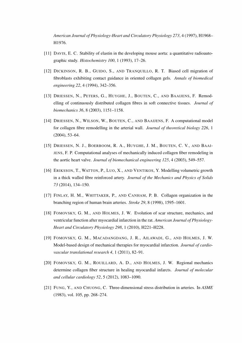
American Journal of Physiology-Heart and Circulatory Physiology 273, 4 (1997), H1968–
H1976.
[11] DAVIS, E. C. Stability of elastin in the developing mouse aorta: a quantitative radioauto-
graphic study. Histochemistry 100, 1 (1993), 17–26.
[12] DICKINSON, R. B., GUIDO, S., AND TRANQUILLO, R. T. Biased cell migration of
fibroblasts exhibiting contact guidance in oriented collagen gels. Annals of biomedical
engineering 22, 4 (1994), 342–356.
[13] DRIESSEN, N., PETERS, G., HUYGHE, J., BOUTEN, C., AND BAAIJENS, F. Remod-
elling of continuously distributed collagen fibres in soft connective tissues. Journal of
biomechanics 36, 8 (2003), 1151–1158.
[14] DRIESSEN, N., WILSON, W., BOUTEN, C., AND BAAIJENS, F. A computational model
for collagen fibre remodelling in the arterial wall. Journal of theoretical biology 226, 1
(2004), 53–64.
[15] DRIESSEN, N. J., BOERBOOM, R. A., HUYGHE, J. M., BOUTEN, C. V., AND BAAI-
JENS, F. P. Computational analyses of mechanically induced collagen fiber remodeling in
the aortic heart valve. Journal of biomechanical engineering 125, 4 (2003), 549–557.
[16] ERIKSSON, T., WATTON, P., LUO, X., AND VENTIKOS, Y. Modelling volumetric growth
in a thick walled fibre reinforced artery. Journal of the Mechanics and Physics of Solids
73 (2014), 134–150.
[17] FINLAY, H. M., WHITTAKER, P., AND CANHAM, P. B. Collagen organization in the
branching region of human brain arteries. Stroke 29, 8 (1998), 1595–1601.
[18] FOMOVSKY, G. M., AND HOLMES, J. W. Evolution of scar structure, mechanics, and
ventricular function after myocardial infarction in the rat. American Journal of Physiology-
Heart and Circulatory Physiology 298, 1 (2010), H221–H228.
[19] FOMOVSKY, G. M., MACADANGDANG, J. R., AILAWADI, G., AND HOLMES, J. W.
Model-based design of mechanical therapies for myocardial infarction. Journal of cardio-
vascular translational research 4, 1 (2011), 82–91.
[20] FOMOVSKY, G. M., ROUILLARD, A. D., AND HOLMES, J. W. Regional mechanics
determine collagen fiber structure in healing myocardial infarcts. Journal of molecular
and cellular cardiology 52, 5 (2012), 1083–1090.
[21] FUNG, Y., AND CHUONG, C. Three-dimensional stress distribution in arteries. In ASME
(1983), vol. 105, pp. 268–274.
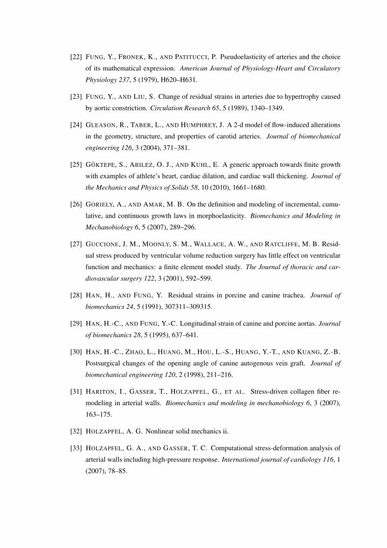
[22] FUNG, Y., FRONEK, K., AND PATITUCCI, P. Pseudoelasticity of arteries and the choice
of its mathematical expression. American Journal of Physiology-Heart and Circulatory
Physiology 237, 5 (1979), H620–H631.
[23] FUNG, Y., AND LIU, S. Change of residual strains in arteries due to hypertrophy caused
by aortic constriction. Circulation Research 65, 5 (1989), 1340–1349.
[24] GLEASON, R., TABER, L., AND HUMPHREY, J. A 2-d model of flow-induced alterations
in the geometry, structure, and properties of carotid arteries. Journal of biomechanical
engineering 126, 3 (2004), 371–381.
[25] GOKTEPE, S., ABILEZ, O. J., AND KUHL, E. A generic approach towards finite growth
with examples of athlete’s heart, cardiac dilation, and cardiac wall thickening. Journal of
the Mechanics and Physics of Solids 58, 10 (2010), 1661–1680.
[26] GORIELY, A., AND AMAR, M. B. On the definition and modeling of incremental, cumu-
lative, and continuous growth laws in morphoelasticity. Biomechanics and Modeling in
Mechanobiology 6, 5 (2007), 289–296.
[27] GUCCIONE, J. M., MOONLY, S. M., WALLACE, A. W., AND RATCLIFFE, M. B. Resid-
ual stress produced by ventricular volume reduction surgery has little effect on ventricular
function and mechanics: a finite element model study. The Journal of thoracic and car-
diovascular surgery 122, 3 (2001), 592–599.
[28] HAN, H., AND FUNG, Y. Residual strains in porcine and canine trachea. Journal of
biomechanics 24, 5 (1991), 307311–309315.
[29] HAN, H.-C., AND FUNG, Y.-C. Longitudinal strain of canine and porcine aortas. Journal
of biomechanics 28, 5 (1995), 637–641.
[30] HAN, H.-C., ZHAO, L., HUANG, M., HOU, L.-S., HUANG, Y.-T., AND KUANG, Z.-B.
Postsurgical changes of the opening angle of canine autogenous vein graft. Journal of
biomechanical engineering 120, 2 (1998), 211–216.
[31] HARITON, I., GASSER, T., HOLZAPFEL, G., ET AL. Stress-driven collagen fiber re-
modeling in arterial walls. Biomechanics and modeling in mechanobiology 6, 3 (2007),
163–175.
[32] HOLZAPFEL, A. G. Nonlinear solid mechanics ii.
[33] HOLZAPFEL, G. A., AND GASSER, T. C. Computational stress-deformation analysis of
arterial walls including high-pressure response. International journal of cardiology 116, 1
(2007), 78–85.
[34] HOLZAPFEL, G. A., GASSER, T. C., AND OGDEN, R. W. A new constitutive frame-
work for arterial wall mechanics and a comparative study of material models. Journal of
elasticity and the physical science of solids 61, 1-3 (2000), 1–48.
[35] HOLZAPFEL, G. A., AND OGDEN, R. W. Constitutive modelling of passive myocardium:
a structurally based framework for material characterization. Philosophical Transactions
of the Royal Society of London A: Mathematical, Physical and Engineering Sciences 367,
1902 (2009), 3445–3475.
[36] HOLZAPFEL, G. A., AND OGDEN, R. W. Modelling the layer-specific three-dimensional
residual stresses in arteries, with an application to the human aorta. Journal of the Royal
Society Interface (2009), rsif20090357.
[37] HOLZAPFEL, G. A., AND OGDEN, R. W. On the tension–compression switch in soft
fibrous solids. European Journal of Mechanics-A/Solids 49 (2015), 561–569.
[38] HOLZAPFEL, G. A., AND OGDEN, R. W. On fiber dispersion models: Exclusion of
compressed fibers and spurious model comparisons. Journal of Elasticity (2016), 1–20.
[39] HOLZAPFEL, G. A., SOMMER, G., AUER, M., REGITNIG, P., AND OGDEN, R. W.
Layer-specific 3d residual deformations of human aortas with non-atherosclerotic intimal
thickening. Annals of biomedical engineering 35, 4 (2007), 530–545.
[40] HSU, F.-H. The influences of mechanical loads on the form of a growing elastic body.
Journal of biomechanics 1, 4 (1968), 303–311.
[41] HUISKES, R., RUIMERMAN, R., VAN LENTHE, G. H., AND JANSSEN, J. D. Effects of
mechanical forces on maintenance and adaptation of form in trabecular bone. Nature 405,
6787 (2000), 704–706.
[42] HUISMAN, R., SIPKEMA, P., WESTERHOF, N., AND ELZINGA, G. Comparison of mod-
els used to calculate left ventricular wall force. Medical and Biological Engineering and
Computing 18, 2 (1980), 133–144.
[43] HUMPHREY, J., AND HOLZAPFEL, G. A. Mechanics, mechanobiology, and modeling of
human abdominal aorta and aneurysms. Journal of biomechanics 45, 5 (2012), 805–814.
[44] HUMPHREY, J., AND RAJAGOPAL, K. A constrained mixture model for growth and re-
modeling of soft tissues. Mathematical models and methods in applied sciences 12, 03
(2002), 407–430.
[45] KARSAJ, I., SORIC, J., AND HUMPHREY, J. D. A 3-d framework for arterial growth and
remodeling in response to altered hemodynamics. International journal of engineering
science 48, 11 (2010), 1357–1372.
[46] KERCKHOFFS, R. C. Computational modeling of cardiac growth in the post-natal rat with
a strain-based growth law. Journal of biomechanics 45, 5 (2012), 865–871.
[47] KERCKHOFFS, R. C., OMENS, J. H., AND MCCULLOCH, A. D. A single strain-based
growth law predicts concentric and eccentric cardiac growth during pressure and volume
overload. Mechanics research communications 42 (2012), 40–50.
[48] KLEPACH, D., LEE, L. C., WENK, J. F., RATCLIFFE, M. B., ZOHDI, T. I., NAVIA,
J. L., KASSAB, G. S., KUHL, E., AND GUCCIONE, J. M. Growth and remodeling of the
left ventricle: a case study of myocardial infarction and surgical ventricular restoration.
Mechanics research communications 42 (2012), 134–141.
[49] KROON, M. A continuum mechanics framework and a constitutive model for remodelling
of collagen gels and collagenous tissues. Journal of the Mechanics and Physics of Solids
58, 6 (2010), 918–933.
[50] KROON, W., DELHAAS, T., ARTS, T., AND BOVENDEERD, P. Computational modeling
of volumetric soft tissue growth: application to the cardiac left ventricle. Biomechanics
and modeling in mechanobiology 8, 4 (2009), 301–309.
[51] LEGRICE, I. J., SMAILL, B., CHAI, L., EDGAR, S., GAVIN, J., AND HUNTER, P. J.
Laminar structure of the heart: ventricular myocyte arrangement and connective tissue
architecture in the dog. American Journal of Physiology-Heart and Circulatory Physiology
269, 2 (1995), H571–H582.
[52] LIU, S., AND FUNG, Y. Zero-stress states of arteries. Journal of biomechanical engineer-
ing 110, 1 (1988), 82–84.
[53] MCDOUGALL, S., DALLON, J., SHERRATT, J., AND MAINI, P. Fibroblast migration and
collagen deposition during dermal wound healing: mathematical modelling and clinical
implications. Philosophical Transactions of the Royal Society of London A: Mathematical,
Physical and Engineering Sciences 364, 1843 (2006), 1385–1405.
[54] MENZEL, A., AND KUHL, E. Frontiers in growth and remodeling. Mechanics research
communications 42 (2012), 1–14.
[55] MERODIO, J., OGDEN, R. W., AND RODRIGUEZ, J. The influence of residual stress on
finite deformation elastic response. International Journal of Non-Linear Mechanics 56
(2013), 43–49.
[56] NOVAK, V. P., YIN, F., AND HUMPHREY, J. Regional mechanical properties of passive
myocardium. Journal of biomechanics 27, 4 (1994), 403–412.
[57] OGDEN, R. W. Non-linear elastic deformations. Courier Corporation, 1997.
[58] OLSSON, T., AND KLARBRING, A. Residual stresses in soft tissue as a consequence
of growth and remodeling: application to an arterial geometry. European Journal of
Mechanics-A/Solids 27, 6 (2008), 959–974.
[59] OMENS, J., MCCULLOCH, A., AND CRISCIONE, J. Complex distributions of residual
stress and strain in the mouse left ventricle: experimental and theoretical models. Biome-
chanics and modeling in mechanobiology 1, 4 (2003), 267–277.
[60] OMENS, J. H., AND FUNG, Y.-C. Residual strain in rat left ventricle. Circulation Re-
search 66, 1 (1990), 37–45.
[61] OMENS, J. H., MACKENNA, D. A., AND MCCULLOCH, A. D. Measurement of strain
and analysis of stress in resting rat left ventricular myocardium. Journal of biomechanics
26, 6 (1993), 665–676.
[62] POOLE, K., KHAIRY, K., FRIEDRICHS, J., FRANZ, C., CISNEROS, D. A., HOWARD, J.,
AND MUELLER, D. Molecular-scale topographic cues induce the orientation and direc-
tional movement of fibroblasts on two-dimensional collagen surfaces. Journal of molecular
biology 349, 2 (2005), 380–386.
[63] RACHEV, A., KANE, T., AND MEISTER, J. Experimental investigation of the distribution
of residual strains in the artery wall.
[64] REN, J.-S. Growth and residual stresses of arterial walls. Journal of theoretical biology
337 (2013), 80–88.
[65] RODRIGUEZ, E. K., HOGER, A., AND MCCULLOCH, A. D. Stress-dependent finite
growth in soft elastic tissues. Journal of biomechanics 27, 4 (1994), 455–467.
[66] ROUILLARD, A. D., AND HOLMES, J. W. Mechanical regulation of fibroblast migration
and collagen remodelling in healing myocardial infarcts. The Journal of physiology 590,
18 (2012), 4585–4602.
[67] ROUILLARD, A. D., AND HOLMES, J. W. Coupled agent-based and finite-element mod-
els for predicting scar structure following myocardial infarction. Progress in biophysics
and molecular biology 115, 2 (2014), 235–243.
[68] SAEZ, P., PENA, E., MARTINEZ, M. A., AND KUHL, E. Computational modeling of
hypertensive growth in the human carotid artery. Computational mechanics 53, 6 (2014),
1183–1196.
[69] SCHMID, H., WATTON, P., MAURER, M., WIMMER, J., WINKLER, P., WANG, Y.,
ROHRLE, O., AND ITSKOV, M. Impact of transmural heterogeneities on arterial adapta-
tion. Biomechanics and modeling in mechanobiology 9, 3 (2010), 295–315.
[70] SCHRIEFL, A. J., REINISCH, A. J., SANKARAN, S., PIERCE, D. M., AND HOLZAPFEL,
G. A. Quantitative assessment of collagen fibre orientations from two-dimensional images
of soft biological tissues. Journal of The Royal Society Interface 9, 76 (2012), 3081–3093.
[71] SHAMS, M., DESTRADE, M., AND OGDEN, R. W. Initial stresses in elastic solids: con-
stitutive laws and acoustoelasticity. Wave Motion 48, 7 (2011), 552–567.
[72] SKALAK, R. Growth as a finite displacement field. In Proceedings of the IUTAM sympo-
sium on finite elasticity (1981), Springer, pp. 347–355.
[73] TABER, L. A model for aortic growth based on fluid shear and fiber stresses.
TRANSACTIONS-AMERICAN SOCIETY OF MECHANICAL ENGINEERS JOURNAL OF
BIOMECHANICAL ENGINEERING 120 (1998), 348–354.
[74] TABER, L., AND CHABERT, S. Theoretical and experimental study of growth and remod-
eling in the developing heart. Biomechanics and modeling in mechanobiology 1, 1 (2002),
29–43.
[75] TABER, L. A. Biomechanics of cardiovascular development. Annual review of biomedical
engineering 3, 1 (2001), 1–25.
[76] TABER, L. A., AND EGGERS, D. W. Theoretical study of stress-modulated growth in the
aorta. Journal of theoretical biology 180, 4 (1996), 343–357.
[77] TABER, L. A., HU, N., PEXIEDER, T., CLARK, E. B., AND KELLER, B. B. Residual
strain in the ventricle of the stage 16-24 chick embryo. Circulation research 72, 2 (1993),
455–462.
[78] TABER, L. A., AND HUMPHREY, J. D. Stress-modulated growth, residual stress, and
vascular heterogeneity. Journal of biomechanical engineering 123, 6 (2001), 528–535.
[79] TAKAMIZAWA, K., AND HAYASHI, K. Strain energy density function and uniform strain
hypothesis for arterial mechanics. Journal of biomechanics 20, 1 (1987), 7–17.
[80] TSAMIS, A., CHENG, A., NGUYEN, T. C., LANGER, F., MILLER, D. C., AND KUHL,
E. Kinematics of cardiac growth: in vivo characterization of growth tensors and strains.
Journal of the mechanical behavior of biomedical materials 8 (2012), 165–177.
[81] UNTERBERGER, M. J., SCHMOLLER, K. M., BAUSCH, A. R., AND HOLZAPFEL, G. A.
A new approach to model cross-linked actin networks: multi-scale continuum formulation
and computational analysis. journal of the mechanical behavior of biomedical materials
22 (2013), 95–114.
[82] VAISHNAV, R. N., YOUNG, J. T., AND PATEL, D. J. Distribution of stresses and of strain-
energy density through the wall thickness in a canine aortic segment. Circulation research
32, 5 (1973), 577–583.
[83] VALENTIN, A., AND HUMPHREY, J. Evaluation of fundamental hypotheses underlying
constrained mixture models of arterial growth and remodelling. Philosophical Transac-
tions of the Royal Society of London A: Mathematical, Physical and Engineering Sciences
367, 1902 (2009), 3585–3606.
[84] VALENTIN, A., HUMPHREY, J., AND HOLZAPFEL, G. A. A finite element-based con-
strained mixture implementation for arterial growth, remodeling, and adaptation: Theory
and numerical verification. International journal for numerical methods in biomedical
engineering 29, 8 (2013), 822–849.
[85] VANDIVER, R. Effect of residual stress on peak cap stress in arteries. Mathematical
biosciences and engineering: MBE 11, 5 (2014), 1199–1214.
[86] VOLOKH, K. Stresses in growing soft tissues. Acta Biomaterialia 2, 5 (2006), 493–504.
[87] VON MALTZAHN, W. W., WARRIYAR, R. G., AND KEITZER, W. F. Experimental mea-
surements of elastic properties of media and adventitia of bovine carotid arteries. Journal
of biomechanics 17, 11 (1984), 839–847.
[88] VOSSOUGHI, J., HEDJAZI, Z., AND BORRIS, F. Intimal residual stress and strain in large
arteries. ASME-PUBLICATIONS-BED 24 (1993), 434–434.
[89] WANG, H., GAO, H., LUO, X., BERRY, C., GRIFFITH, B., OGDEN, R., AND WANG, T.
Structure-based finite strain modelling of the human left ventricle in diastole. International
journal for numerical methods in biomedical engineering 29, 1 (2013), 83–103.
[90] WANG, H., LUO, X., GAO, H., OGDEN, R., GRIFFITH, B., BERRY, C., AND WANG, T.
A modified holzapfel-ogden law for a residually stressed finite strain model of the human
left ventricle in diastole. Biomechanics and modeling in mechanobiology 13, 1 (2014),
99–113.
[91] WANG, V. Y., HUSSAN, J. R., YOUSEFI, H., BRADLEY, C. P., HUNTER, P. J., AND
NASH, M. P. Modelling cardiac tissue growth and remodelling. Journal of Elasticity 129,
1-2 (2017), 283–305.
[92] WATTON, P., AND HILL, N. Evolving mechanical properties of a model of abdominal
aortic aneurysm. Biomechanics and modeling in mechanobiology 8, 1 (2009), 25–42.
[93] WATTON, P., HILL, N., AND HEIL, M. A mathematical model for the growth of the
abdominal aortic aneurysm. Biomechanics and modeling in mechanobiology 3, 2 (2004),
98–113.
[94] WATTON, P. N., VENTIKOS, Y., AND HOLZAPFEL, G. A. Modelling the growth and
stabilization of cerebral aneurysms. Mathematical Medicine and Biology 26, 2 (2009),
133–164.
[95] WONG, J., AND KUHL, E. Generating fibre orientation maps in human heart models using
poisson interpolation. Computer methods in biomechanics and biomedical engineering 17,
11 (2014), 1217–1226.
[96] YIN, F. C. Ventricular wall stress. Circulation Research 49, 4 (1981), 829–842.